CovBSM: An Optimization Approach to RF Beacon Deployment forIndoor Localization

Raphael Falque1, Mitesh Patel2, and Jacob Biehl2

Abstract— In this paper, we propose a novel solution tooptimize the deployment of Radio Frequency (RF) beacons forthe purpose of indoor localization. We propose a system thatoptimizes both the number of beacons and their placementin a given environment. We propose a novel cost-function,called CovBSM, that allows to simultaneously optimize the 3-coverage while maximizing the beacon spreading. Using thiscost function, we propose a framework that maximize both thenumber of beacons and their placement in a given environment.The proposed solution accounts for the indoor infrastructureand its influence on the RF signal propagation by embeddinga realistic simulator into the optimization process.

Keywords: Indoor localization, Beacon deployment, Blue-tooth Low Energy (BLE), k-Coverage, Wireless sensor networks(WSN).

I. INTRODUCTIONLocalization problems can be solved effectively using

Global Navigation Satellite Systems (GNSS). However, forindoor localization, GNSS is most often not available. As analternative, localization solutions using different modalitiessuch as RGB-D cameras [1], Inertial Measurement Unit(IMU) [2], and wireless access point (Wi-Fi) [3] have beendeveloped by various researchers. Additionally, researchershave also developed multi-modal localization approaches byfusing two or more sensors [4], [5].

With wireless communication technologies becomingwidespread and ubiquitous, they have been studied exten-sively as a solution to indoor positioning systems [6]. Varioussolutions based on the Bluetooth Low Energy (BLE) technol-ogy [5], [7] have been proposed. Most often, these methodsuse the Received Signal Strength Indication (RSSI) fromthe BLE beacons to estimates the user position. In indoorenvironments, the radio signals are severely impacted due toshadowing and multipathing effects which lead to noisy data.To receive better RSSI signal from BLEs, they are placed inlocations where RSSI signals are available through Line-Of-Sight (LOS) thereby going through minimal multipathing.

Scaling BLE based indoor positioning becomes a challeng-ing problem as it involves placing beacons at the optimallocation to get a high level of localization accuracy. Inmost of the indoor positioning systems [5], [7], beaconsare placed using expert knowledge about the environmentalcondition in order to achieve good localization accuracy.Hence the optimal placement of BLE beacons has beenstudied by researchers from the Wireless Sensor Network

1Raphael Falque is with Centre for Autonomous System, Faculty of Engi-neering and IT, University of Technology Sydney, Ultimo, NSW 2007, Aus-tralia Raphael.H.Guenot-Falque@student.uts.edu.au

2Mitesh Patel, and Jacob Biehl are with FX Palo Alto Laboratory Inc.,Palo Alto, CA - 94304, USA {mitesh,biehl}@fxpal.com

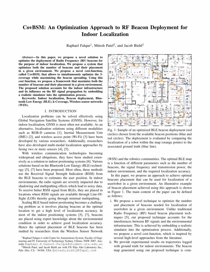
Fig. 1: Sample of an optimized BLE beacon deployment (redcircles) chosen from the available beacon positions (blue andred circles). The deployment is evaluated by comparing thelocalization of a robot within the map (orange points) to theassociated ground truth (blue line).

(WSN) and the robotics communities. The optimal BLE mapis a function of different parameters such as the number ofbeacons, the signal frequency and transmission power, theindoor environment, and the required localization accuracy.

In this paper, we propose an approach to achieve optimalbeacons placement that can be used for localization of auser/robot in a given environment. An illustrative exampleof beacon placement achieved using this approach is shownin Figure 1. The main content of the paper can be definedas follows:

i. We propose a novel technique to optimize the numberand placement of beacons needed for localization ofuser/robot in a given environment. Unlike traditionalRadio Frequency (RF) based beacon placement tech-niques [5], our proposed technique accounts for theinterferences between RF signals and the environmentalinfrastructure. This is achieved by embedding a realisticsimulator into the optimization process. Additionally,we propose a novel cost-function, which is inspired byseveral high-level approaches from the literature.

ii. We provide experimental results on trajectories loggedwith ground truth for indoor environments. The beaconmap generated using our proposed technique is com-

pared to a deployment designed by human operatorswhere beacons are deployed in all the power plugsavailable. The results generated using the beacon mapis evaluated with different localization techniques suchas Linear Least Square (LLS) and Particle Filter (PF).Through our experiments, we demonstrate that the num-ber of required beacons were reduced by 53% whilereducing the localization accuracy by only 0.6 m com-pared to the results obtained when using the completedistribution of beacons.

II. RELATED WORK

The optimization of landmarks/beacons placement forindoor localization on a predefined path is well studied inthe literature. Using the prior of a predefined path, near-optimal solutions can be obtained with greedy approaches.These methods incrementally add beacons at the locationsthat minimize the localization uncertainty [8] or some otherconfidence bounds, such as a guaranty of minimum deviationfrom the desired path [9]. As an alternative to a predefinedpath, it is also possible to consider a set of trajectoriessimilarly to the approach proposed by [10] where the visuallandmarks are iteratively added while considering a set ofindependent trajectories. Despite providing bounds related tothe localization performances, these methods require a pathknown in advance to formulate the optimization problem.Hence, they are not practical for human localization orunplanned exploration of a floorplan.

In cases where the path followed by the robot/user isunknown, one can use the methods developed by the WSNresearch community and to formulate the problem as acoverage problem (in this case the sensors are replaced by theset of beacon emitters). Solutions to the coverage problemhave been surveyed by Wang et al. [11] and a standardapproach is to use regular lattices in order to design thedeployment of the WSN. The evaluation of different lattices’pattern (e.g., square grid, hexagonal lattice) has been studiedby Chen et al. using trilateration and they concluded that adeployment based on a triangular lattice is the best patternfor localization tasks.

Similarly, it is possible to formulate the coverage problemas an art gallery problem which is known to be NP-hard. In such case, meta-heuristics strategies such as Ge-netic Algorithm (GA) offer good candidates to find near-optimal solution [12]. In this context, Yoon et al. developedan efficient variant of GA which has better performancesthan standards GA approaches for the specific case of thecoverage problem [13]. Evaluation of their technique wasdone with Monte Carlo simulations. Similarly, Seo et al.used GA to optimize the sensor placement in a battlefieldenvironment with a GPU implementation to achieve max-imum coverage [14]. The authors divided the terrain intoa grid and calculated the probability of vehicle detectionusing generational GA when it passes through to each cell.Similarly, Carter and Ragade use a probabilistic model thataccounts for the detection probabilities of the sensing devices

which may decay with distance, environmental conditionsand hardware configurations [15].

While the aforementioned methods provide potential solu-tions, the coverage problem is not designed to optimize theplacement of landmarks for localization purpose. Therefore,other metrics such as the Geometric Dilution Of Precision(GDOP), which was originally defined in order to quan-tify the quality of the satellite positioning for localizationpurpose, can provide better information for optimizing thebeacon deployment. Roa et al. have shown that a beacondeployment based on the optimization of the GDOP canoutperform regular lattices [16]. The optimization of theGDOP on a floorplan has been done for different modalities,such as angular emitters used for tiangulation [17] and morerecently, Rajagopal et al. introduced the concept of UniquelyLocalizable (UL) which can be combined to GDOP for thedeployment of sound beacons [18]. The deployment hasbeen tested on simulated datasets; however, this conceptseems incompatible with the through wall propagation ofRF beacons.

An alternative approach has been proposed by Zou etal. in the Virtual Force Algorithm (VFA). This methoditeratively updates the position of beacons by moving themaway or towards each other according to the inter-sensordistances [19]. Once optimized, the algorithm would ideallyreach a configuration where all beacon are spaced by apredefined distance. They evaluate the performance of theVFA by using the beacon deployment for localization pur-pose. Their localization approach is based on matching thesensor readings at any given point of the environment witha predefined probabilistic table.

Most of the literature does not account properly for theenvironment in the optimization of the beacon deployment.The methods that maximize the inter-beacon distances areinherently independent of the environment. The other meth-ods optimizing the coverage are often based on simplesensor models that do not account for the environment. Ourproposed approach differs from the prior methods in thefollowing ways:

i. Our proposed system optimizes for both the number ofbeacons required in a given environment and optimizingthe location of those beacons.

ii. We propose a novel cost-function that combines the k-coverage methods and the beacon spreading.

iii. Our proposed system is generalized whereby it accountsfor beacon placement constraints due to environmentalconditions as well as noisy signal characteristics due tomulti-path issues.

III. PROBLEM DEFINITION

In this paper, we consider the deployment of BLE beaconsfor indoor localization. We consider both the problem offinding the number, n, of beacons required, and the search oftheir optimal placements in order to maximize localizationaccuracy. We define B to be the space where the beacons canbe deployed and B the set of the chosen beacons’ position,

start: B = ∅

Generate apopulation of b

Simulates eachb with PyLayer

Cost-functionevaluation

Is bbestimproving?

Evolve the setof candidate

Genetic algorithm

assign bbest into B

Globaltermination

criterion met?

return: B

Yes

No

No

yes

Fig. 2: Initial greedy deployment

which is more formally defined as B = {b1, ..., bn} withbi ∈ B the ith beacon position.

IV. METHODOLOGY

During the deployment stage, the number of BLE beaconsrequired to cover an area is often unknown. Estimating thisquantity is often a hard task as the required number ofbeacon depends on the environment. Therefore, we first use agreedy algorithm to estimate the number of beacons required.Once this quantity is known, we then consider a globaloptimization formulation to obtain a more optimal solution.

A. Algorithm architecture

We first explain the architecture of the main algorithmbefore providing more details for each part of the algorithmin the following sub-sections.

The proposed greedy algorithm initializes the set of de-ployed beacon B as an empty set. A GA is then used to findthe beacon position that would maximize our cost-functionfCovBSM. In other words, the added beacon bbest is defined asargmax

b(fCovBSM(B ∪ b)). The process is repeated iteratively

until a termination criterion is met. The flowchart of thegreedy algorithm is shown in Figure 2.

As the previous greedy approach can not be optimal [20],we perform a re-deployment step using the number ofbeacons obtained from the greedy approach. As shown

Define apopulation of B

Simulate beaconswith PyLayer

Cost-functionevaluation

Is Bbestimproving?

Evolve the setof candidate

Genetic algorithm

return: B

Yes

No

Fig. 3: Global re-deployment

in Figure 3, the approach is quite similar to the greedyapproach. However, conversely to the greedy approach wherethe optimized parameter is a single beacon location b, wenow consider the optimization of a full set of beacons loca-tions, i.e., the optimized parameter is now B = {b1, ..., bn}with n the number of beacons obtained from the greedyapproach.

In the following sub-section we explain how the sensormodel is defined. We then provide the definition of the cost-function which is built on top of the sensor model. Finallywe explain how the GA algorithm optimizes the sensorplacement using the cost-function.

B. Sensor modeling

As discussed in [21], different sensor models can be usedto model the propagation of BLE beacon over a 2D plan. Themodels commonly used in the literature are the disk model,the Friis model1, and the direct LOS model. The behaviorof these models for a simple scenario is shown in Figure 4.

While some of these models are a good approximation ofthe sensor behavior in an open environment — especially thedisk model — they are a bad approximation of the reality in

1The Friis model is also referred to as the probabilistic model andexponential model.

(a) (b) (c)

Fig. 4: Sensor model commonly used in the literature: in (a)the disk model, in (b) the Friis model [22], and in (c) thedirect line-of-sight model.

(a) (b)

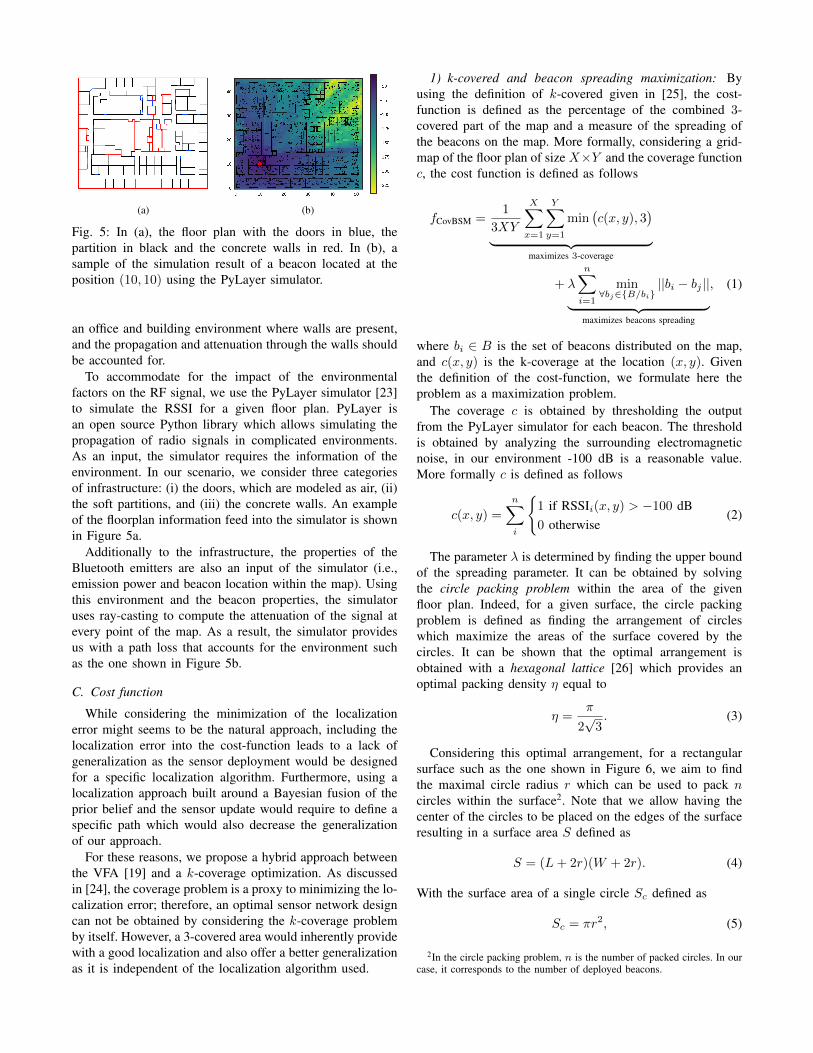
Fig. 5: In (a), the floor plan with the doors in blue, thepartition in black and the concrete walls in red. In (b), asample of the simulation result of a beacon located at theposition (10, 10) using the PyLayer simulator.

an office and building environment where walls are present,and the propagation and attenuation through the walls shouldbe accounted for.

To accommodate for the impact of the environmentalfactors on the RF signal, we use the PyLayer simulator [23]to simulate the RSSI for a given floor plan. PyLayer isan open source Python library which allows simulating thepropagation of radio signals in complicated environments.As an input, the simulator requires the information of theenvironment. In our scenario, we consider three categoriesof infrastructure: (i) the doors, which are modeled as air, (ii)the soft partitions, and (iii) the concrete walls. An exampleof the floorplan information feed into the simulator is shownin Figure 5a.

Additionally to the infrastructure, the properties of theBluetooth emitters are also an input of the simulator (i.e.,emission power and beacon location within the map). Usingthis environment and the beacon properties, the simulatoruses ray-casting to compute the attenuation of the signal atevery point of the map. As a result, the simulator providesus with a path loss that accounts for the environment suchas the one shown in Figure 5b.

C. Cost function

While considering the minimization of the localizationerror might seems to be the natural approach, including thelocalization error into the cost-function leads to a lack ofgeneralization as the sensor deployment would be designedfor a specific localization algorithm. Furthermore, using alocalization approach built around a Bayesian fusion of theprior belief and the sensor update would require to define aspecific path which would also decrease the generalizationof our approach.

For these reasons, we propose a hybrid approach betweenthe VFA [19] and a k-coverage optimization. As discussedin [24], the coverage problem is a proxy to minimizing the lo-calization error; therefore, an optimal sensor network designcan not be obtained by considering the k-coverage problemby itself. However, a 3-covered area would inherently providewith a good localization and also offer a better generalizationas it is independent of the localization algorithm used.

1) k-covered and beacon spreading maximization: Byusing the definition of k-covered given in [25], the cost-function is defined as the percentage of the combined 3-covered part of the map and a measure of the spreading ofthe beacons on the map. More formally, considering a grid-map of the floor plan of size X×Y and the coverage functionc, the cost function is defined as follows

fCovBSM =1

3XY

X∑x=1

Y∑y=1

min(c(x, y), 3

)︸ ︷︷ ︸

maximizes 3-coverage

+ λ

n∑i=1

min∀bj∈{B/bi}

||bi − bj ||︸ ︷︷ ︸maximizes beacons spreading

, (1)

where bi ∈ B is the set of beacons distributed on the map,and c(x, y) is the k-coverage at the location (x, y). Giventhe definition of the cost-function, we formulate here theproblem as a maximization problem.

The coverage c is obtained by thresholding the outputfrom the PyLayer simulator for each beacon. The thresholdis obtained by analyzing the surrounding electromagneticnoise, in our environment -100 dB is a reasonable value.More formally c is defined as follows

c(x, y) =

n∑i

{1 if RSSIi(x, y) > −100 dB0 otherwise

(2)

The parameter λ is determined by finding the upper boundof the spreading parameter. It can be obtained by solvingthe circle packing problem within the area of the givenfloor plan. Indeed, for a given surface, the circle packingproblem is defined as finding the arrangement of circleswhich maximize the areas of the surface covered by thecircles. It can be shown that the optimal arrangement isobtained with a hexagonal lattice [26] which provides anoptimal packing density η equal to

η =π

2√3. (3)

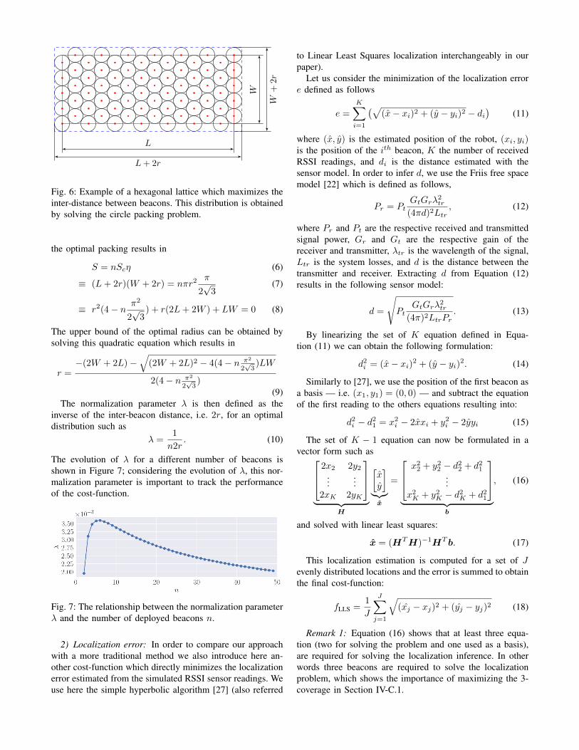
Considering this optimal arrangement, for a rectangularsurface such as the one shown in Figure 6, we aim to findthe maximal circle radius r which can be used to pack ncircles within the surface2. Note that we allow having thecenter of the circles to be placed on the edges of the surfaceresulting in a surface area S defined as

S = (L+ 2r)(W + 2r). (4)

With the surface area of a single circle Sc defined as

Sc = πr2, (5)

2In the circle packing problem, n is the number of packed circles. In ourcase, it corresponds to the number of deployed beacons.

L

L+ 2r

W

W+2r

Fig. 6: Example of a hexagonal lattice which maximizes theinter-distance between beacons. This distribution is obtainedby solving the circle packing problem.

the optimal packing results in

S = nScη (6)

≡ (L+ 2r)(W + 2r) = nπr2π

2√3

(7)

≡ r2(4− n π2

2√3) + r(2L+ 2W ) + LW = 0 (8)

The upper bound of the optimal radius can be obtained bysolving this quadratic equation which results in

r =−(2W + 2L)−

√(2W + 2L)2 − 4(4− n π2

2√3)LW

2(4− n π2

2√3)

(9)The normalization parameter λ is then defined as the

inverse of the inter-beacon distance, i.e. 2r, for an optimaldistribution such as

λ =1

n2r. (10)

The evolution of λ for a different number of beacons isshown in Figure 7; considering the evolution of λ, this nor-malization parameter is important to track the performanceof the cost-function.

Fig. 7: The relationship between the normalization parameterλ and the number of deployed beacons n.

2) Localization error: In order to compare our approachwith a more traditional method we also introduce here an-other cost-function which directly minimizes the localizationerror estimated from the simulated RSSI sensor readings. Weuse here the simple hyperbolic algorithm [27] (also referred

to Linear Least Squares localization interchangeably in ourpaper).

Let us consider the minimization of the localization errore defined as follows

e =

K∑i=1

(√(x− xi)2 + (y − yi)2 − di

)(11)

where (x, y) is the estimated position of the robot, (xi, yi)is the position of the ith beacon, K the number of receivedRSSI readings, and di is the distance estimated with thesensor model. In order to infer d, we use the Friis free spacemodel [22] which is defined as follows,

Pr = PtGtGrλ

2tr

(4πd)2Ltr, (12)

where Pr and Pt are the respective received and transmittedsignal power, Gr and Gt are the respective gain of thereceiver and transmitter, λtr is the wavelength of the signal,Ltr is the system losses, and d is the distance between thetransmitter and receiver. Extracting d from Equation (12)results in the following sensor model:

d =

√Pt

GtGrλ2tr(4π)2LtrPr

. (13)

By linearizing the set of K equation defined in Equa-tion (11) we can obtain the following formulation:

d2i = (x− xi)2 + (y − yi)2. (14)

Similarly to [27], we use the position of the first beacon asa basis — i.e. (x1, y1) = (0, 0) — and subtract the equationof the first reading to the others equations resulting into:

d2i − d21 = x2i − 2xxi + y2i − 2yyi (15)

The set of K − 1 equation can now be formulated in avector form such as 2x2 2y2

......

2xK 2yK

︸ ︷︷ ︸

H

[xy

]︸︷︷︸x

=

x22 + y22 − d22 + d21...

x2K + y2K − d2K + d21

︸ ︷︷ ︸

b

, (16)

and solved with linear least squares:

x = (HTH)−1HT b. (17)

This localization estimation is computed for a set of Jevenly distributed locations and the error is summed to obtainthe final cost-function:

fLLS =1

J

J∑j=1

√(xj − xj)2 + (yj − yj)2 (18)

Remark 1: Equation (16) shows that at least three equa-tion (two for solving the problem and one used as a basis),are required for solving the localization inference. In otherwords three beacons are required to solve the localizationproblem, which shows the importance of maximizing the 3-coverage in Section IV-C.1.

D. Genetic algorithm

Considering the sensor model used herein (i.e. the PyLayersimulator), having a search approach which is agnosticfrom the cost-function helps avoiding gradient computation.Indeed, as the sensor is modeled using a simulator, thecomputation of an analytical gradient is not possible. For thisreason and the arguments related to metaheuristics providedin the related work section, we use a GA for optimizing oursolutions. We used the DEAP library for the implementationof the GA optimization [28].

GA is an optimization process inspired by Darwin’s theoryof evolution. In the GA’s terminology, the parameters arereferred as genomes, the full set of parameters that forma solution of the optimization problem is called individual,and the set of individuals is called population. The GAoptimization starts by an initialization of the population. Anevaluation of the population is then performed with the cost-function mentioned in the previous section, and given theresults of the evaluation, a selection process is executed inorder to keep the good candidates. An evolution strategy isthen performed by using crossover and mutation. The processis then iteratively repeated from the evaluation stage.

The crossover consists of switching parameters betweendifferent individuals. The crossover is characterized by ahyperparameter called the probability of crossover. The mu-tation consists of adding noise to the parameters values andis characterized by the probability of mutation. In practice,the crossover is used in order to jump to another place in thespace of the parameters and is similar to the jumping in basinhoping. The mutation is used to explore the neighborhoodof the good candidates.

Once the GA is setup, we embed it into the systemsdescribed in Figure 2 and 3 to find the required quantity ofbeacons and where to deploy the beacons. Specific examplesof the GA parametrization is given in the following section.

V. EXPERIMENTAL RESULTS

In this section, we introduce the results of both thegreedy and global optimization. The datasets collected inour experiment are available upon request.

A. Experimental setup

The evaluation of the proposed approach is done byconsidering the performance of two different localizationsalgorithms given the optimized beacons deployment in thereal world. The environment used for evaluation is an indooroffice-like space of size 40×50 m2 shown in Figure 8b. Weuse a robotic platform in order to collect both the ground-truth and the Bluetooth RSSI measurement.

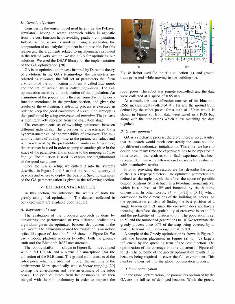
The robotic platform — shown in Figure 8a — is equippedwith a 2D LIDAR and a Nexus 6P smartphone (for thecollection of the BLE data). The ground truth consists of therobot poses which are obtained through the mapping of theenvironment. More specifically, we use hector mapping [29]to map the environment and have an estimate of the robotposes. The pose estimates from hector mapping are thenmerged with the robot odometry in order to improve the

(a) (b)

Fig. 8: Robot used for the data collection (a), and groundtruth generated while moving in the building (b).

robot poses. The robot was remote controlled, and the datawere collected at a speed of 0.65 m·s−1.

As a result, the data collection consists of the bluetoothRSSI measurements collected at 7 Hz and the ground truthdefined by the robot poses, for a path of 150 m which isshown in Figure 8b. Both data were saved in a ROS bagalong with the timestamps which allow matching the datatogether.

B. Greedy approach

GA is a stochastic process; therefore, there is no guaranteethat the search would reach consistently the same solutionfor different randomizer initialization. Therefore, we have todecide how many time the experiment has to be repeated inorder to claim the result as valid. Each experiment has beenrepeated 50 times with different random seeds for evaluationwith quantitative results.

Prior to providing the results, we first describe the setupof the GA’s hyperparameters. The optimized parameters aredefined as the tuple (x, y); therefore, the space of possiblebeacon positions B is defined as a two-dimensional intervalwhich is a subset of R2 and bounded by the buildingdimensions. In other words, B = [0, 51] × [0, 41] whichcorrespond to the dimensions of the building in meters. Asthe optimization consists of finding the best position of asingle beacon on a 2D map, the crossover does not have ameaning; therefore, the probability of crossover is set to 0.0and the probability of mutation to 0.3. The population is setto 50 and the number of generations to 10. We terminate thegreedy process once 90% of the map being covered by atleast 3 beacons, i.e. 3-coverage equal to 0.9.

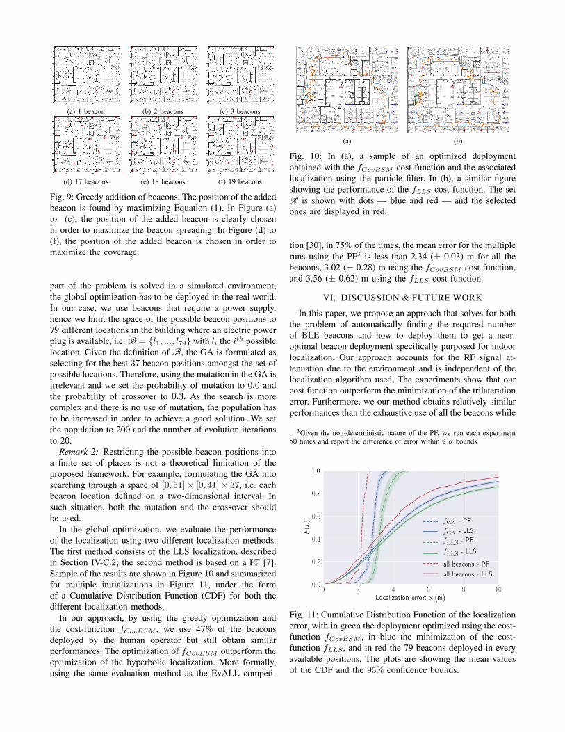
A sample of the Greedy optimization is shown in Figure 9,with the beacon placement in Figure (a) to (c) largelyinfluenced by the spreading term of the cost function. Theoptimization of the coverage is more apparent in Figure (d)to (f). The outcome of the greedy optimization results in 37beacons being required to cover the full environment. Thisnumber is then fed into the global optimization process.

C. Global optimization

In the global optimization, the parameters optimized by theGA are the full set of deployed beacons. While the greedy

(a) 1 beacon (b) 2 beacons (c) 3 beacons

(d) 17 beacons (e) 18 beacons (f) 19 beacons

Fig. 9: Greedy addition of beacons. The position of the addedbeacon is found by maximizing Equation (1). In Figure (a)to (c), the position of the added beacon is clearly chosenin order to maximize the beacon spreading. In Figure (d) to(f), the position of the added beacon is chosen in order tomaximize the coverage.

part of the problem is solved in a simulated environment,the global optimization has to be deployed in the real world.In our case, we use beacons that require a power supply,hence we limit the space of the possible beacon positions to79 different locations in the building where an electric powerplug is available, i.e. B = {l1, ..., l79} with li the ith possiblelocation. Given the definition of B, the GA is formulated asselecting for the best 37 beacon positions amongst the set ofpossible locations. Therefore, using the mutation in the GA isirrelevant and we set the probability of mutation to 0.0 andthe probability of crossover to 0.3. As the search is morecomplex and there is no use of mutation, the population hasto be increased in order to achieve a good solution. We setthe population to 200 and the number of evolution iterationsto 20.

Remark 2: Restricting the possible beacon positions intoa finite set of places is not a theoretical limitation of theproposed framework. For example, formulating the GA intosearching through a space of [0, 51]× [0, 41]× 37, i.e. eachbeacon location defined on a two-dimensional interval. Insuch situation, both the mutation and the crossover shouldbe used.

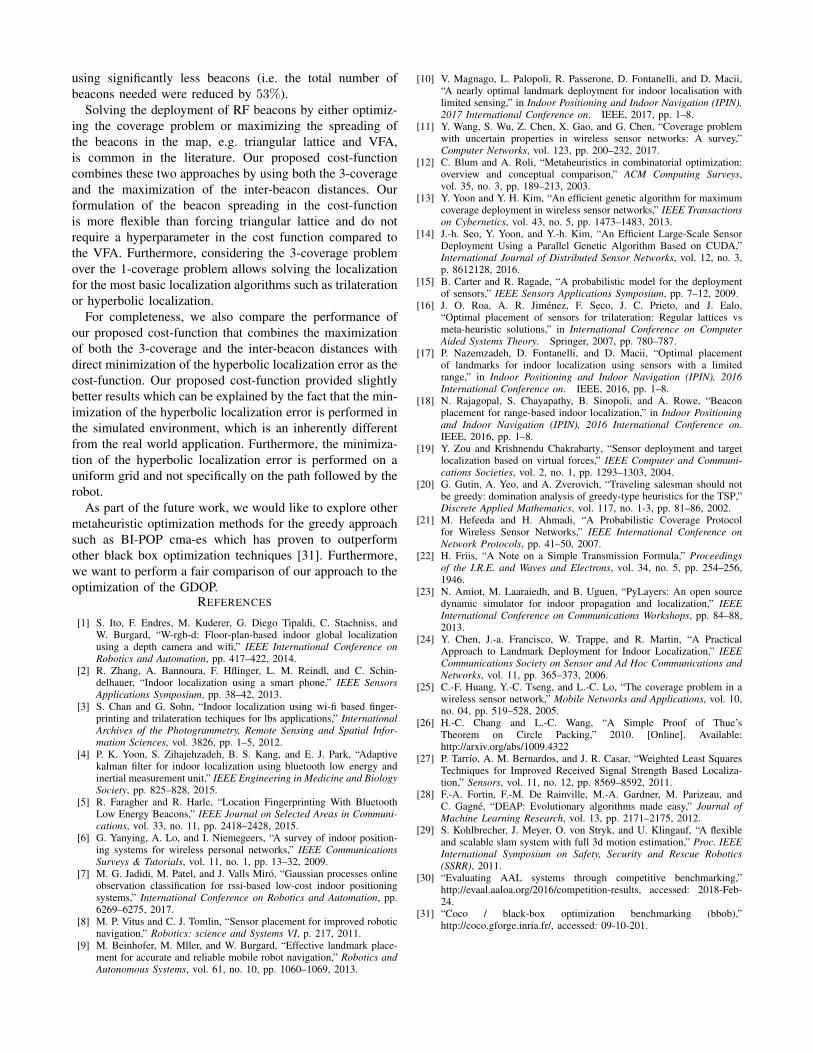
In the global optimization, we evaluate the performanceof the localization using two different localization methods.The first method consists of the LLS localization, describedin Section IV-C.2; the second method is based on a PF [7].Sample of the results are shown in Figure 10 and summarizedfor multiple initializations in Figure 11, under the formof a Cumulative Distribution Function (CDF) for both thedifferent localization methods.

In our approach, by using the greedy optimization andthe cost-function fCovBSM , we use 47% of the beaconsdeployed by the human operator but still obtain similarperformances. The optimization of fCovBSM outperform theoptimization of the hyperbolic localization. More formally,using the same evaluation method as the EvALL competi-

(a) (b)

Fig. 10: In (a), a sample of an optimized deploymentobtained with the fCovBSM cost-function and the associatedlocalization using the particle filter. In (b), a similar figureshowing the performance of the fLLS cost-function. The setB is shown with dots — blue and red — and the selectedones are displayed in red.

tion [30], in 75% of the times, the mean error for the multipleruns using the PF3 is less than 2.34 (± 0.03) m for all thebeacons, 3.02 (± 0.28) m using the fCovBSM cost-function,and 3.56 (± 0.62) m using the fLLS cost-function.

VI. DISCUSSION & FUTURE WORK

In this paper, we propose an approach that solves for boththe problem of automatically finding the required numberof BLE beacons and how to deploy them to get a near-optimal beacon deployment specifically purposed for indoorlocalization. Our approach accounts for the RF signal at-tenuation due to the environment and is independent of thelocalization algorithm used. The experiments show that ourcost function outperform the minimization of the trilaterationerror. Furthermore, we our method obtains relatively similarperformances than the exhaustive use of all the beacons while

3Given the non-deterministic nature of the PF, we run each experiment50 times and report the difference of error within 2 σ bounds

Fig. 11: Cumulative Distribution Function of the localizationerror, with in green the deployment optimized using the cost-function fCovBSM , in blue the minimization of the cost-function fLLS , and in red the 79 beacons deployed in everyavailable positions. The plots are showing the mean valuesof the CDF and the 95% confidence bounds.

using significantly less beacons (i.e. the total number ofbeacons needed were reduced by 53%).

Solving the deployment of RF beacons by either optimiz-ing the coverage problem or maximizing the spreading ofthe beacons in the map, e.g. triangular lattice and VFA,is common in the literature. Our proposed cost-functioncombines these two approaches by using both the 3-coverageand the maximization of the inter-beacon distances. Ourformulation of the beacon spreading in the cost-functionis more flexible than forcing triangular lattice and do notrequire a hyperparameter in the cost function compared tothe VFA. Furthermore, considering the 3-coverage problemover the 1-coverage problem allows solving the localizationfor the most basic localization algorithms such as trilaterationor hyperbolic localization.

For completeness, we also compare the performance ofour proposed cost-function that combines the maximizationof both the 3-coverage and the inter-beacon distances withdirect minimization of the hyperbolic localization error as thecost-function. Our proposed cost-function provided slightlybetter results which can be explained by the fact that the min-imization of the hyperbolic localization error is performed inthe simulated environment, which is an inherently differentfrom the real world application. Furthermore, the minimiza-tion of the hyperbolic localization error is performed on auniform grid and not specifically on the path followed by therobot.

As part of the future work, we would like to explore othermetaheuristic optimization methods for the greedy approachsuch as BI-POP cma-es which has proven to outperformother black box optimization techniques [31]. Furthermore,we want to perform a fair comparison of our approach to theoptimization of the GDOP.

REFERENCES

[1] S. Ito, F. Endres, M. Kuderer, G. Diego Tipaldi, C. Stachniss, andW. Burgard, “W-rgb-d: Floor-plan-based indoor global localizationusing a depth camera and wifi,” IEEE International Conference onRobotics and Automation, pp. 417–422, 2014.

[2] R. Zhang, A. Bannoura, F. Hflinger, L. M. Reindl, and C. Schin-delhauer, “Indoor localization using a smart phone,” IEEE SensorsApplications Symposium, pp. 38–42, 2013.

[3] S. Chan and G. Sohn, “Indoor localization using wi-fi based finger-printing and trilateration techiques for lbs applications,” InternationalArchives of the Photogrammetry, Remote Sensing and Spatial Infor-mation Sciences, vol. 3826, pp. 1–5, 2012.

[4] P. K. Yoon, S. Zihajehzadeh, B. S. Kang, and E. J. Park, “Adaptivekalman filter for indoor localization using bluetooth low energy andinertial measurement unit,” IEEE Engineering in Medicine and BiologySociety, pp. 825–828, 2015.

[5] R. Faragher and R. Harle, “Location Fingerprinting With BluetoothLow Energy Beacons,” IEEE Journal on Selected Areas in Communi-cations, vol. 33, no. 11, pp. 2418–2428, 2015.

[6] G. Yanying, A. Lo, and I. Niemegeers, “A survey of indoor position-ing systems for wireless personal networks,” IEEE CommunicationsSurveys & Tutorials, vol. 11, no. 1, pp. 13–32, 2009.

[7] M. G. Jadidi, M. Patel, and J. Valls Miro, “Gaussian processes onlineobservation classification for rssi-based low-cost indoor positioningsystems,” International Conference on Robotics and Automation, pp.6269–6275, 2017.

[8] M. P. Vitus and C. J. Tomlin, “Sensor placement for improved roboticnavigation,” Robotics: science and Systems VI, p. 217, 2011.

[9] M. Beinhofer, M. Mller, and W. Burgard, “Effective landmark place-ment for accurate and reliable mobile robot navigation,” Robotics andAutonomous Systems, vol. 61, no. 10, pp. 1060–1069, 2013.

[10] V. Magnago, L. Palopoli, R. Passerone, D. Fontanelli, and D. Macii,“A nearly optimal landmark deployment for indoor localisation withlimited sensing,” in Indoor Positioning and Indoor Navigation (IPIN),2017 International Conference on. IEEE, 2017, pp. 1–8.

[11] Y. Wang, S. Wu, Z. Chen, X. Gao, and G. Chen, “Coverage problemwith uncertain properties in wireless sensor networks: A survey,”Computer Networks, vol. 123, pp. 200–232, 2017.

[12] C. Blum and A. Roli, “Metaheuristics in combinatorial optimization:overview and conceptual comparison,” ACM Computing Surveys,vol. 35, no. 3, pp. 189–213, 2003.

[13] Y. Yoon and Y. H. Kim, “An efficient genetic algorithm for maximumcoverage deployment in wireless sensor networks,” IEEE Transactionson Cybernetics, vol. 43, no. 5, pp. 1473–1483, 2013.

[14] J.-h. Seo, Y. Yoon, and Y.-h. Kim, “An Efficient Large-Scale SensorDeployment Using a Parallel Genetic Algorithm Based on CUDA,”International Journal of Distributed Sensor Networks, vol. 12, no. 3,p. 8612128, 2016.

[15] B. Carter and R. Ragade, “A probabilistic model for the deploymentof sensors,” IEEE Sensors Applications Symposium, pp. 7–12, 2009.

[16] J. O. Roa, A. R. Jimenez, F. Seco, J. C. Prieto, and J. Ealo,“Optimal placement of sensors for trilateration: Regular lattices vsmeta-heuristic solutions,” in International Conference on ComputerAided Systems Theory. Springer, 2007, pp. 780–787.

[17] P. Nazemzadeh, D. Fontanelli, and D. Macii, “Optimal placementof landmarks for indoor localization using sensors with a limitedrange,” in Indoor Positioning and Indoor Navigation (IPIN), 2016International Conference on. IEEE, 2016, pp. 1–8.

[18] N. Rajagopal, S. Chayapathy, B. Sinopoli, and A. Rowe, “Beaconplacement for range-based indoor localization,” in Indoor Positioningand Indoor Navigation (IPIN), 2016 International Conference on.IEEE, 2016, pp. 1–8.

[19] Y. Zou and Krishnendu Chakrabarty, “Sensor deployment and targetlocalization based on virtual forces,” IEEE Computer and Communi-cations Societies, vol. 2, no. 1, pp. 1293–1303, 2004.

[20] G. Gutin, A. Yeo, and A. Zverovich, “Traveling salesman should notbe greedy: domination analysis of greedy-type heuristics for the TSP,”Discrete Applied Mathematics, vol. 117, no. 1-3, pp. 81–86, 2002.

[21] M. Hefeeda and H. Ahmadi, “A Probabilistic Coverage Protocolfor Wireless Sensor Networks,” IEEE International Conference onNetwork Protocols, pp. 41–50, 2007.

[22] H. Friis, “A Note on a Simple Transmission Formula,” Proceedingsof the I.R.E. and Waves and Electrons, vol. 34, no. 5, pp. 254–256,1946.

[23] N. Amiot, M. Laaraiedh, and B. Uguen, “PyLayers: An open sourcedynamic simulator for indoor propagation and localization,” IEEEInternational Conference on Communications Workshops, pp. 84–88,2013.

[24] Y. Chen, J.-a. Francisco, W. Trappe, and R. Martin, “A PracticalApproach to Landmark Deployment for Indoor Localization,” IEEECommunications Society on Sensor and Ad Hoc Communications andNetworks, vol. 11, pp. 365–373, 2006.

[25] C.-F. Huang, Y.-C. Tseng, and L.-C. Lo, “The coverage problem in awireless sensor network,” Mobile Networks and Applications, vol. 10,no. 04, pp. 519–528, 2005.

[26] H.-C. Chang and L.-C. Wang, “A Simple Proof of Thue’sTheorem on Circle Packing,” 2010. [Online]. Available:http://arxiv.org/abs/1009.4322

[27] P. Tarrıo, A. M. Bernardos, and J. R. Casar, “Weighted Least SquaresTechniques for Improved Received Signal Strength Based Localiza-tion,” Sensors, vol. 11, no. 12, pp. 8569–8592, 2011.

[28] F.-A. Fortin, F.-M. De Rainville, M.-A. Gardner, M. Parizeau, andC. Gagne, “DEAP: Evolutionary algorithms made easy,” Journal ofMachine Learning Research, vol. 13, pp. 2171–2175, 2012.

[29] S. Kohlbrecher, J. Meyer, O. von Stryk, and U. Klingauf, “A flexibleand scalable slam system with full 3d motion estimation,” Proc. IEEEInternational Symposium on Safety, Security and Rescue Robotics(SSRR), 2011.

[30] “Evaluating AAL systems through competitive benchmarking,”http://evaal.aaloa.org/2016/competition-results, accessed: 2018-Feb-24.

[31] “Coco / black-box optimization benchmarking (bbob),”http://coco.gforge.inria.fr/, accessed: 09-10-201.