Course web page: week posting... · Chap 8 Chap Chap 3 Chap 7 Scan Read Pages Pages Pages ... Real...

Course web page: http://Stanford2008.pageout.net

Handout #10

Foreign Exchange MarketsExchange Rate Forecasting

Slides to highlight: 1-39, 71-107.

MWF 3:15-4:30 Gates B01on Wednesday July 16, 2008

8-2

Levich

Luenberger

Solnik

Blanchard

Wooldridge

Chap 8

Chap

Chap 3

Chap 7

Scan Read

Pages

Pages

Pages

Pages

Chap Pages

Foreign Exchange Determination and Forecasting

Exchange Rate Forecasting

Multiple Regression Analysis with Qualitative Information: Binary (or Dummy) Variables

Reading Assignments for this Week

Foreign Exchange MarketsExchange Rate Forecasting

MS&E 247S International InvestmentsYee-Tien Fu

8-4

EXCHANGE RATE FORECASTING

“My father was in the import-export business and he used to ask me to predict exchange rates. It’s an experience that did not bring us much closer.”

- University economist speaking at conferenceon international finance

8-5

The Importance of Exchange Rate Forecasting

Exchange rate forecasts plays a fundamental role in nearly all aspects of international financial management.- Short-term hedging or cash management decisions often rely on a forecast of expected exchange rate movements.- To evaluate foreign borrowing or investment opportunities, forecasts of future spot exchange rates are necessary to convert expected foreign currency cash flows into their expected domestic currencies.

8-6

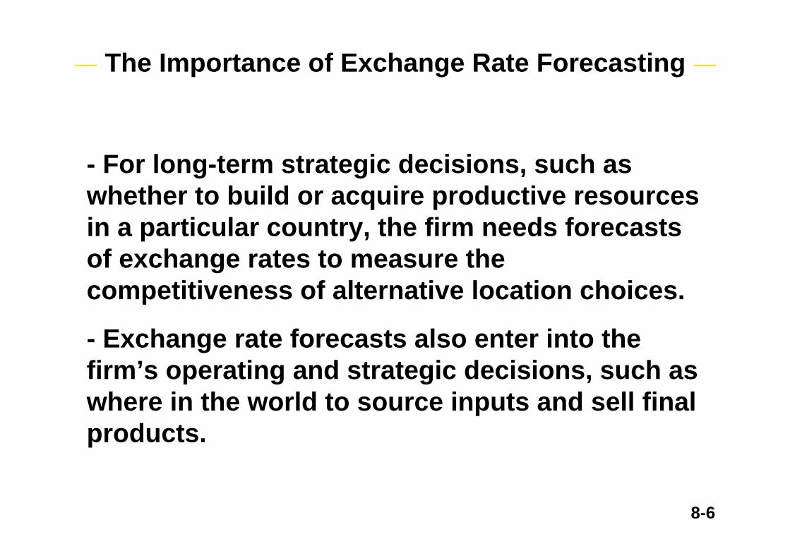
- For long-term strategic decisions, such as whether to build or acquire productive resources in a particular country, the firm needs forecasts of exchange rates to measure the competitiveness of alternative location choices.


- Exchange rate forecasts also enter into the firm’s operating and strategic decisions, such as where in the world to source inputs and sell final products.

8-7

However, there is considerable skepticism about the possibility of accurate or useful forecasts:- If economists are not able to describe the fundamental determinants of exchange rates, clearly economic models will not be very helpful for forecasting.


- If markets are efficient, and prices fully reflect all available information, including structural economic information, then unanticipated exchange rate movements are only the results of unanticipated events - and by definition, these cannot be forecasted.

8-8

Recently, several well-known economists have summarized this pessimistic view regarding our ability to explain exchange rate movements after the fact, or to forecast exchange rate change before the fact.


8-9

A FRAMEWORK FOR FORECASTING EXCHANGE RATES

Factors Examples1. Exchange Rate Systems

Pegged Bretton Woods periodFloating Post-Bretton Woods period

for many major countriesHybrid systems Bloc pegging [such as the

European MonetarySystem], managed floating, target zones

The Bretton Woods system gave a central role to gold.

8-10

Pegged Exchange Rate Regime

- An exchange rate between two countries is allowed to vary within narrow bands.- Is maintained ultimately by central bank intervention at the upper and lower intervention points.- Central bank intervention is supported by international reserves which each country holds in finite supply.

- As long as the inflationary experience of the countries is similar, the pegged rate may be sustained.

8-11

- A prolonged period of inflation differences precedes a change in the international competitiveness of our countries, leading to a current account deficit and a loss of reserves in the higher inflation country. This situation is not sustainable in the long run.


8-12

- Once an exchange rate becomes misaligned, the likely direction of change in the exchange rate is fairly easy to predict: depreciation in countries that have experienced losses in international reserves, excess inflation and current account deficit, and appreciation where there has been relatively low inflation and current account surpluses. It also may be possible to infer the likely magnitude of change in the exchange rate needed to restore equilibrium.


8-13

- The deviation from purchasing power parity offers one natural estimate of the likely exchange rate change.- The PPP equilibrium rate can be computed in many ways: using different base years, base periods, and price indexes. So there is no unique PPP rate.- Economic models offer little guidance about the timing of change since the decision to adjust the peg is typically a political decision. As such, the political party in power may resist a depreciation of the peg.


8-14

Bilson (1979) examined a monetary model of the exchange rate and an international liquidity variable (measured as the stock of international reserves relative to the monetary base) as indicators of discrete exchange rate changes.

- Economists have attempted to model the political and economic events that might presage an exchange rate change.

- Found that the monetary model frequently offers a good proxy for the magnitude of devaluation.


8-15

- Found that the international liquidity ratio provides a leading indicator of the actual devaluation date.- Examples for three devaluations of Latin American currencies showed that when the international liquidity indicator falls substantially relative to its historical norm, the actual exchange rate depreciates thereafter within one or two years.- The two indicators appear to offer exchange rate forecasters some useful information.


8-16

Special Drawing Rights (SDRs)

SDRs are book entries that are credited to the accounts of IMF member countries according to their established quotas. They can be used to meet payments imbalances, and they provide a net addition to the stock of reserves without the need for any country to run deficits or mine gold.The SDR was originally set equal in value to the gold content of a U.S. dollar in 1969, which was 0.888571 grams, or 1/35 oz. The value was later revised, first being based on a weighted basket of 16 currencies and subsequently being simplified to 5 currencies. The amount of each currency and the U.S. dollar equivalents are shown in the table on the next slide.

8-17

Special Drawing Rights (SDRs)

The currency basket and the weights are revised every 5 years according to the importance of each country in international trade. The value of the SDR is quoted daily.

DeutschemarkFrench francJapanese yenPound sterlingU.S. dollar

0.45300.0800

31.80000.08120.5720

0.26590.13240.31500.11890.5720

Currency Currency Amount U.S.$ Equivalent

Total $1.4042 = SDR1Source: IMF Treasurer’s Department, August 16, 1993

8-18http://www.imf.org/external/np/tre/sdr/basket.htm

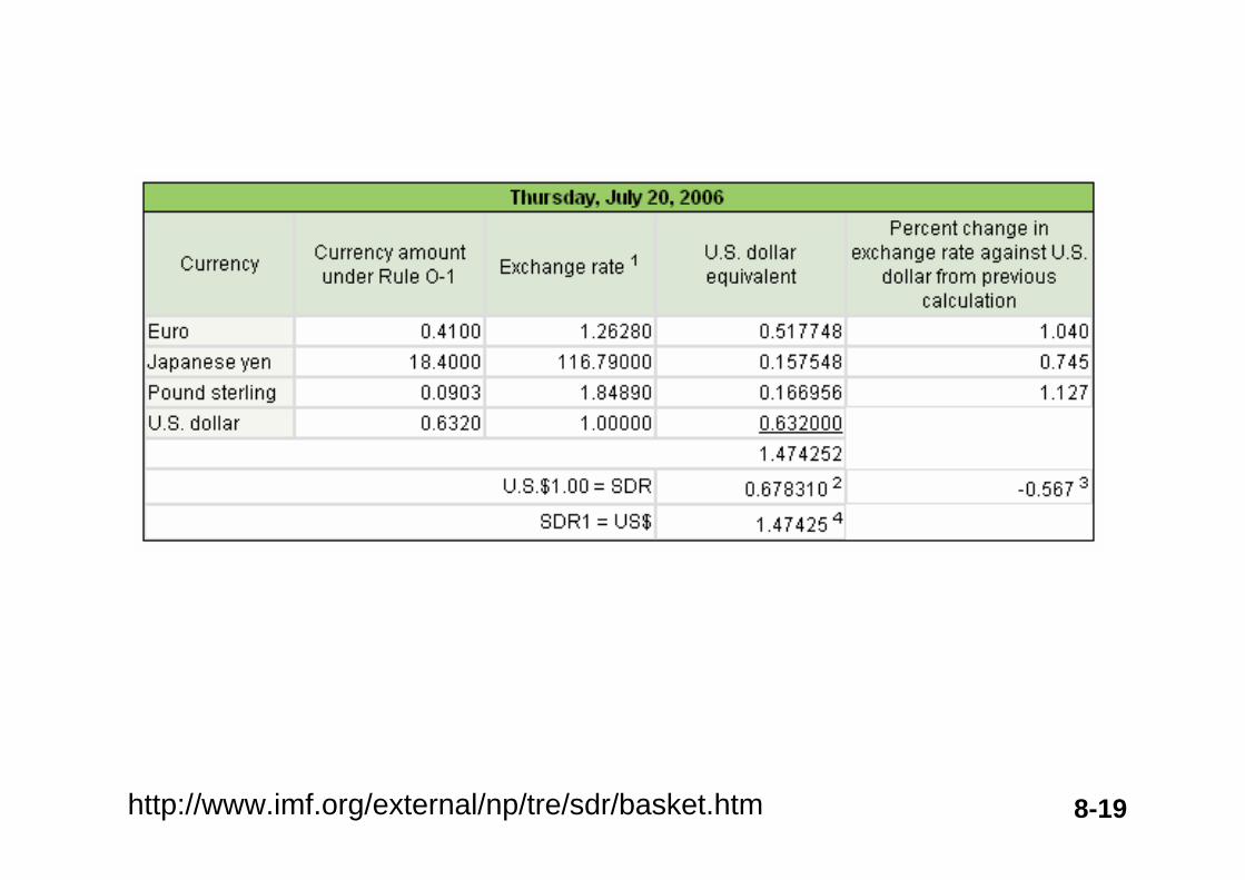
8-19http://www.imf.org/external/np/tre/sdr/basket.htm

8-20

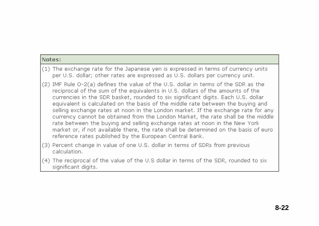
(1) The exchange rate for the Japanese yen is expressed in terms of currency units per U.S. dollar; other rates are expressed as U.S. dollars per currency unit.

(2) IMF Rule O-2(a) defines the value of the U.S. dollar in terms of the SDR as the reciprocal of the sum of the equivalents in U.S. dollars of the amounts of the currencies in the SDR basket, rounded to six significant digits. Each U.S. dollar equivalent is calculated on the basis of the middle rate between the buying and selling exchange rates at noon in the London market. If the exchange rate for any currency cannot be obtained from the London Market, the rate shall be the middle rate between the buying and selling exchange rates at noon in the New York market or, if not available there, the rate shall be determined on the basis of euro reference rates published by the European Central Bank.

(3) Percent change in value of one U.S. dollar in terms of SDRs from previous calculation.

(4) The reciprocal of the value of the U.S dollar in terms of the SDR, rounded to six significant digits.

http://www.imf.org/external/np/tre/sdr/basket.htm

8-23

Floating Exchange Rate System

- Under such a system, the exchange rate is free to adjust quickly in response to changing relative macroeconomic conditions.

- A floating exchange rate reflects the speculative dynamics of the market - with prices moving by large amounts in response to unanticipated changes in economic fundamentals, and short-run price movements overshooting their required long-term adjustment.

8-24

- Forecasting in such an environment is easier when the market is efficient in processing available information, but forecasting for profit can be more difficult for the same reason.

Floating Exchange Rate System

8-25

Hybrid Exchange Rate Systems

- Such as the European Monetary System (bloc pegging), a managed floating, or a target zone system.

- Could reflect elements of both the pegged and floating process.

- Under the Exchange Rate Mechanism (ERM) of the European Monetary System, exchange rates are guided primarily by market forces within the upper and lower intervention points.

8-26

- At the extremities of the band, the question of sustainability of the central rate versus realignment becomes critical.

- At the extremities of the band, the “one-way bet” described for pegged rates becomes operative.

- PPP will likely give a reasonable approximation of where the next central rate alignment is headed.


8-27

- The timing of the alignment is uncertain, guided again by economic considerations (such as the stock of international reserves and the willingness to incur intervention losses) and political considerations (such as the strength of the countries commitment to the ERM).


8-28

Factors Examples2. Forecast Horizon

Very short term 1, 2, 3 minutes, hours, daysShort term 1, 2, 3 weeks, monthsMedium term 1, 2, 3 quartersLong term 1, 2, 3 years, decades


8-29

Factors Examples3. Foreign Exchange Units

Nominal Home currency orForeign currency

Real Adjusted for relative inflation, deviations from PPP


8-30

Forecast Performance Evaluation

- The traditional econometric approach begins with the forecast error made at time t, defined as:

jt

jt

SS tat forecast ahead period-j

+

+

+

+

−=

−=

jt

jtjtt S

SSe ,

ˆ

8-31

Intuitively, it seems natural to prefer forecasts that produce smaller errors. Thus criteria such as the following are often adopted as measures of performance.

n

e

MAE

n

e

ME

ii

ii

∑

∑

=

=Mean Error:

Mean Absolute Error:


8-32

n

e

RMSE

n

e

MSE

ii

ii

∑

∑

=

=

2

2

Mean Squared Error:

Root Mean Squared Error:


8-33

It is possible to produce a small mean error as a result of large negative and positive individual errors. Therefore, in practice, the MAE and RMSE are more commonly used to estimates the average error size.


8-34

But all of these traditional measures could be seriously misleading when the forecast is used for financial hedging or speculative purposes.

Consider the forecasts represented below ($/ £ ):

08.2ˆ,02.2,00.2,99.1ˆ 2,

1 ==== +++ ntntntnt SSFS

The present forward rate is $2.00/ £, and two alternative forecasts are 1.99 (forecast 1) and 2.08 (forecast 2). When the future spot rate is realized, let its value be $2.02/£.

8-35

ly.respective 06.0 and 0.03 is ˆ ,ˆ with associatederror The 21 +−SS

Which forecast is more accurate?Conventional analysis ranks 1S as more accurateA closer look reveals that forecast 1 in effect advised speculators to short £ in the forward market, and advised US$-based investors to hedge their long £ positions in advance of a predicted depreciation of £. This hedging and speculative advice was incorrect because £actually appreciated relative to the forward rate (1.99 < 2.00 but 2.02 > 2.00).

8-36

Forecast 2 was not very accurate, but it led to correct and profitable advice: US$-based speculators would have profited by establishing long forward £ positions and US$-based investors should not have hedged their existing long £ positions (2.08 > 2.00 and 2.02 > 2.00).

Comparing forecast 1 and forecast 2, we found that it is important to distinguish between accurate forecasts and useful forecasts.

8-37

Accurate forecasts have small forecasting errors gauged by traditional statistical measures such as the MAE or RMSE.Useful forecasts are those on the “right side of the market” and lead to profitable speculative positions and correct hedging decisions.

To measure how often a forecaster’s advice has been on the “right side of the market,” we must have a measure of “the market.” In the absence of a currency risk premium, “right side of the market” implies “right side of the forward rate.”Thus, useful forecasts are those that lead to correct hedging decisions.

8-38

When a risk premium (RPt,j) is present, the comparison should be drawn to the market’s expected future spot rate (Ft,j - RPt,j) rather than simply the forward rate.

By this measure, forecasts are either “correct”or “incorrect” leading to a simple binomial test for the presence of forecasting expertise or market timing ability.

8-39

Correct

Incorrect

Incorrect

Correct

Actual Exchange Rate Change

PredictedExchangeRateChange

jtjt FS ,>+ jtjt FS ,<+

jtjt FS ,,ˆ >

jtjt FS ,,ˆ <

To begin this test, consider the 2X2 matrix below:

8-40

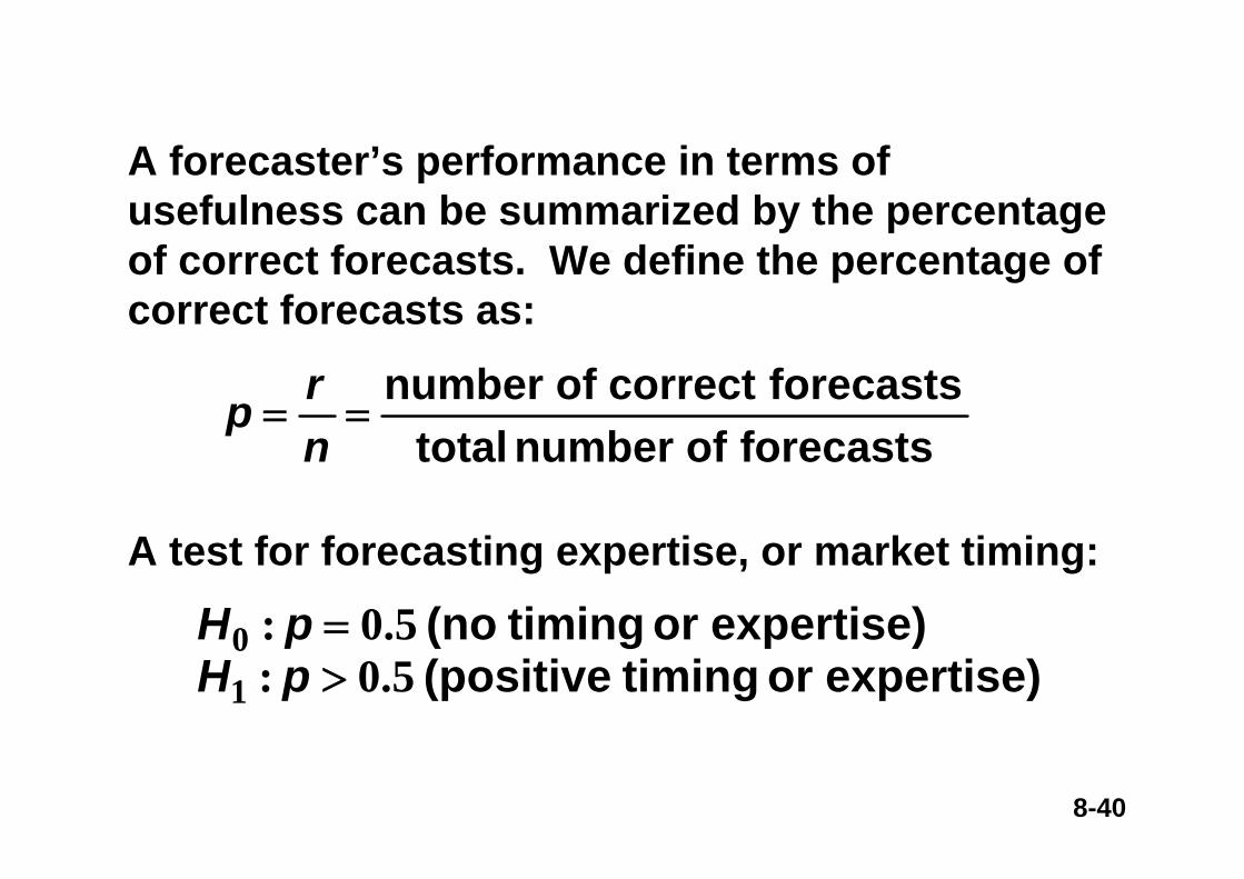
A forecaster’s performance in terms of usefulness can be summarized by the percentage of correct forecasts. We define the percentage of correct forecasts as:

forecasts of number totalforecastscorrect of number

==nrp

A test for forecasting expertise, or market timing:

expertise) or timing (positive expertise) or timing (no

5.0:5.0:

10

>=

pHpH

8-41

Consider a series of n independent trials, each resulting in one of two possible outcomes, “success” or “failure.” Let p = P(success occurs at any given trial) and assume that p remains constant from trial to trial. Let the variable X denote the total number of successes in the n trials. Then X is said to have a binomial distribution and

nkppknk

nkXP knk ..., ,1 ,0 )1()!(!

!)( =−−

== −

)1( )( )(2 pnpXVarnpXE

−==

==

σ

μ

8-42

ExerciseLet X1, X2, …, Xn be a random sample of size n drawn from a population with expected value E(X). The sample mean, denoted X, is the arithmetic average of the Xi’s:

Find E(X).

_

_∑

=

=n

iiX

nX

1

1

8-43

In statistics, we often have to draw inferences based on X, the average computed from a random sample of n observations.Two important properties of X need to be remembered.First, if the Xi’s come from a population whose mean is μ, then E(X) = μ.Second, if the Xi’s come from a population whose variance is σ2, then Var(X) = σ2/n.

_

_

_

_

8-44

Central Limit Theorem: Let Y1, Y2, … be an infinite sequence of independent random variables, each with the same distribution. Suppose that the mean μ and the variance σ2 of fY(y) are both finite. For any numbers c and d,

Larsen & Marx pg 322

dyedn

nYYcPd

c

yn

n∫ −

∞→

=⎟⎠

⎞⎜⎝

⎛ <−+⋅⋅⋅+

<2)2/1(1

21

lim πσμ

8-45

dxednpq

npXcPd

c

x

n ∫−

∞→=<

−< 2

2

21π

)(lim

DeMoivre-Laplace Theorem:Let X be a binomial random variable defined on nindependent trials each having success probability p. For any numbers c and d,

Larsen & Marx pg 206

8-46

Confidence Interval for the Binomial Parameter: given n independent Bernoulli trials, resulting in a total of x successes, construct an interval estimate for the unknown success probability, p.

Apply the DeMoivre-Laplace statement for large n, the quantity below behaves like a standard normal.

2

11n

pp

pnX

npnp

npXX

X

X

)()( −

−=

−−

=−

σμ

8-47

)()(

)(

//

//

22

2

2

2 11

αα

αα α

zZPzZPwhere

z

npp

pnX

zP

≥=−≤

−≅

⎥⎥⎥⎥

⎦

⎤

⎢⎢⎢⎢

⎣

⎡

<−

−<−

Thus

8-48

• Normal distribution¤ A random variable X with mean μ and

variance σ2 is normally distributed if its probability density function is given by

........

)( )])[(/(

7182821415932

1 221

==

∞≤≤∞−= −−

eandwhere

xexf x

ππσ

μ

8-49

• Standard Normal distribution¤ A random variable X with mean μ =0 and

standard deviation σ =1 has standard normal distribution if its probability density function is given by

....eand....where

xef(x) )])[(x/(

718282141593211 2021

==

∞≤≤∞−= −−

ππ

8-50

A bell shaped distribution, symmetrical around μ

μ

8-51

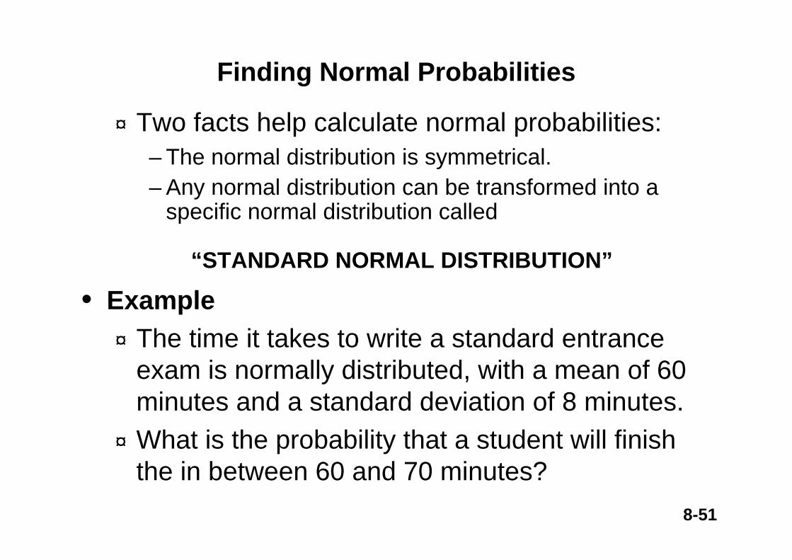
¤ Two facts help calculate normal probabilities:– The normal distribution is symmetrical.– Any normal distribution can be transformed into a

specific normal distribution called

“STANDARD NORMAL DISTRIBUTION”

• Example¤ The time it takes to write a standard entrance

exam is normally distributed, with a mean of 60 minutes and a standard deviation of 8 minutes.

¤ What is the probability that a student will finish the in between 60 and 70 minutes?

Finding Normal Probabilities

8-52

• Solution¤ If X denotes the time taken to write the

exam, we seek the probability P(60<X<70).¤ This probability can be calculated by

creating a new normal variable the standard normal variable.

x

xXZσ

μ−=

E(Z) = 0 V(Z) = 1

Every normal variable with some μ and σ, can be transformed into this Z.

Therefore, once probabilities for Z are calculated, probabilities of any normal variable can found.

8-53

• The symmetry of the normal distribution makes it possible to calculate probabilities for negative values of Z using the table as follows:

-z0 +z00

P(-z0<Z<0) = P(0<Z<z0)

8-54

Sampling Distributions

Basic Statistics Review

Probability and Sampling ReviewSee also slides from Data Analysis I & IIby Robert M Freund, et al.

8-55

• In real life calculating parameters of populations is prohibitive because populations are very large.

• Rather than investigating the whole population, we take a sample, calculate a statistic related to the parameter of interest, and make an inference.

• The sampling distribution of the statistic is the tool that tells us how close is the statistic to the parameter.

8-56

¤ If a random sample is drawn from any population,

¤ the sampling distribution of the sample mean is approximately normal for a sufficiently large sample size.

¤ The larger the sample size, the more closely the sampling distribution of will resemble a normal distribution.

x

The Central Limit Theorem

8-57

size. sample large lysufficient for ddistribute normally elyapproximat is x

nonnormal is x If normal. is x normal, .

.

.

isxIfn

xx

xx

3

2

12

2 σσ

μμ

=

=

The Sampling Distribution of the Sample Mean

8-58

• Example 1¤ The amount of soda pop in each bottle is normally

distributed with a mean of 32.2 ounces and a standard deviation of .3 ounces.

¤ Find the probability that a bottle bought by a customer will contain more than 32 ounces.

¤ Solution– The random variable X is the amount of soda in a

bottle.

7486.0)67.z(P

)3.

2.3232x(P)32x(Px

=−>=

−>

σμ−

=>

μ = 32.2

0.7486

x = 32

8-59

μ = 32.2

0.7486x = 32

¤ Find the probability that a carton of four bottles will have a mean of more than 32 ounces of soda per bottle.

¤ Solution– The random variable here is the mean amount of

soda per bottle.

9082.0)33.1z(P

)43.

2.3232x(P)32x(Px

=−>=

−>

σμ−

=>

32x =

0.9082

2.32x =μ

8-60

• Example 2¤ The average weekly income of graduates one

year after graduation is $600.¤ Suppose the distribution of weekly income has

a standard deviation of $100. What is the probability that 25 randomly selected graduates have an average weekly income of less than $550?

¤ Solution

0062.0)5.2z(P

)25100

600550x(P)550x(Px

=−<=

−<

σμ−

=<

8-61

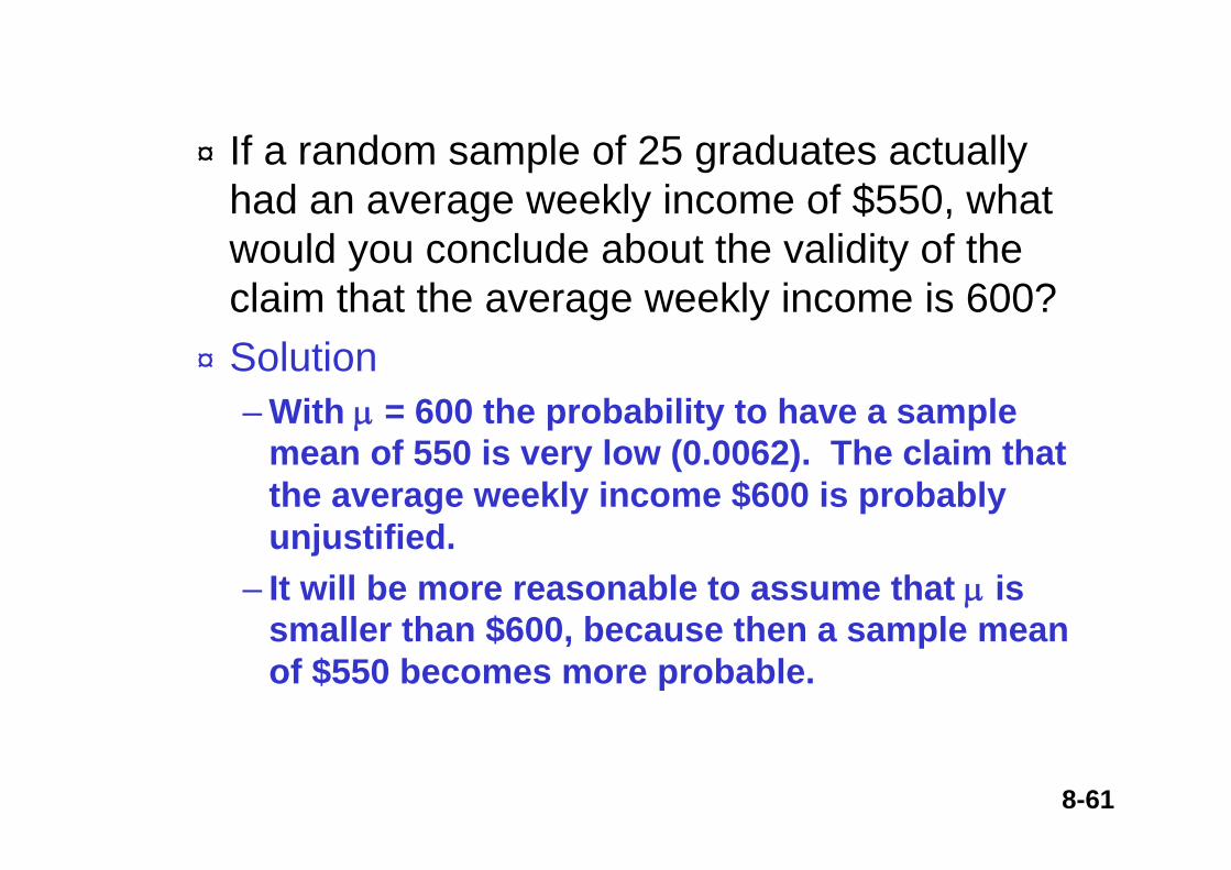
¤ If a random sample of 25 graduates actually had an average weekly income of $550, what would you conclude about the validity of the claim that the average weekly income is 600?

¤ Solution– With μ = 600 the probability to have a sample

mean of 550 is very low (0.0062). The claim that the average weekly income $600 is probably unjustified.

– It will be more reasonable to assume that μ is smaller than $600, because then a sample mean of $550 becomes more probable.

8-62

95.)n

96.1xn

96.1(P

becomewhich

95.)n

96.1xn

96.1(P

aswrirrenbecanThis

95.)96.1n

x96.1(Por,95.)96.1z96.1(P

=σ

+μ≤≤σ

−μ

=σ

≤μ−≤σ

−

=≤σ

μ−≤−=≤≤−

¤ To make inference about population parameters we use sampling distributions (as in example 2).

¤ The symmetry of the normal distribution along with the sample distribution of the mean lead to:

- Z.025 Z.025

Using sampling distributions for inference

8-63

μ

n96.1 σ

−μn

96.1 σ+μ

.025 .025

-1.96 -1.960

.025 .025

Standard normal distribution Z

Normal distribution of x

8-64

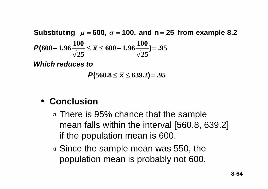
• Conclusion¤ There is 95% chance that the sample

mean falls within the interval [560.8, 639.2] if the population mean is 600.

¤ Since the sample mean was 550, the population mean is probably not 600.

9526398560

9525

10096160025

100961600

.)..(

.)..(

8.2 example from 25n and 100, 600, ngSubstituti

=≤≤

=+≤≤−

===

xPtoreducesWhich

xP

σμ

8-65

In general

α−=σ

+μ≤≤σ

−μ αα 1)n

zxn

z(P 22

8-66

• The parameter of interest for qualitative data is the proportion of times a particular outcome (success) occurs.

• To estimate the population proportion p we use the sample proportion .

• The sampling distribution of is binomial. • We prefer to use normal approximation to

the binomial distribution to make inferences about .

p

Sampling Distribution of a Proportion

p

p

8-67

¤ Normal approximation to the binomial works best when

– the number of experiments (sample size) is large, and– the probability of success, p, is close to 0.5.

¤ For the approximation to provide good results:

np > 5; n(1 - p) > 5

Normal approximation to the Binomial

8-68

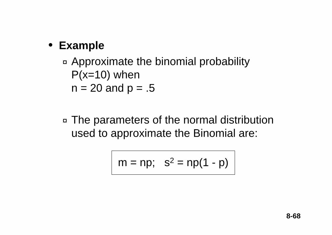
• Example¤ Approximate the binomial probability

P(x=10) when n = 20 and p = .5

¤ The parameters of the normal distribution used to approximate the Binomial are:

m = np; s2 = np(1 - p)

8-69

109.5 10.5

P(XBinomial = 10) ~= P(9.5<Y<10.5)

μ = np = 20(.5) = 10; σ2 = np(1 - p) = 20(.5)(1 - .5) = 5

1742.)24.2

105.10Z24.2

105.9(P =−

≤≤−

=

The exact probability is P(X = 10) = .176

Let us build a normal distribution toapproximate the binomial P(X = 10).

P(9.5<YNormal<10.5)The approximation

8-70

• More normal approximation exercises

P(X<=8) = P(Y< 8.5)

88.5

1413.5

For large n the effects of the continuity correction factor is very small and will be omitted.

P(X>= 14) = P(Y > 13.5)

8-71

¤ From the laws of expected value and variance, it can be shown that E( ) = p and V( ) = p(1-p)/n

¤ If both np > 5 and np(1-p) > 5, then

is approximately standard normally distributed.

p

n)p1(p

ppz−

−=

p p

Approximate sampling distribution of a sample proportion

8-72

• Example 3¤ The Laurier company’s brand has a market

share of 30%. In a survey 1000 consumers were asked which brand they prefer.

¤ What is the probability that more than 32% of all the respondents say they prefer the Laurier brand?

¤ Solution– The number of respondents who prefer Laurier is

binomial with n = 1000 and p = .30. Also, np = 1000(.3) = 300 > 5n(1-p) = 1000(1-.3) = 700 > 5.

0838.01449.

30.32.n)p1(p

ppP)32.p(P =⎟⎟⎠

⎞⎜⎜⎝

⎛ −>

−−

=>

8-73

Forecasting Methods: Some Specific Examples

Short-Run Forecasts: Trends versus Random Walk

Long-Run Forecasts:Reversion to the Mean?

Composite Forecasts: Theory and Examples

8-74


Many economists have concluded that short-run exchange rate movements are nearly random, so that a random-walk (with zero drift) forecast is the best short-run forecast that one can formulate.

At the same time, we have highlighted technical, trend-following models that appear to earn profits from exploiting patterns in spot rates.These results stand in contradiction. How can exchange rates appear random to some researchers, yet display patterns to other researchers?

8-75

The reason is that most studies of exchange rate behavior have used linear regression models below:

(8.1) etrendPasttrendFuture ++= )(10 ββ

and ß1 is typically shown to be insignificantly different from 0; the coefficient of determination R2 (0< R2 <1, R2 measures the proportion of the total variation in LHS that is accounted for by variation in the regressors) of these regressions is generally less than 1% (i.e., the regression provides an unsatisfactory since R2 <<1 here.)


8-76

Hence, these results support a random-walk view - the future trend appears unrelated to the past trend.

Bilson points out that the problem with this methodology is that linear regression analysis assumes a linear (proportionate) relationship.For example, if the past trend movement in the exchange rate is +10 percent, equation (8.1) predicts a larger movement in the future than if the past trend movement in the exchange rate had been only +5 percent.


8-77

Most technical models would make far weaker quantitative predictions: If the exchange rate has gone up (down) in the past, it is likely to go up (down) in the future. Technical models do not impose a linear relationship such as that given in equation (8.1).

Bilson introduced the following dummy variable regression:


8-78

(8.2) 1,991,221,110 ttttt eDDDreturnFuture ++⋅⋅⋅+++= −−− ββββ

Where each dummy variable (Di) takes the value +1 if the past price trend falls within a specified interval, and zero otherwise. For example, D2=1 when the measure of past trend (ΔSt/σ) falls into the interval of (-1.75, -1.25), and D2=0 otherwise.

Equation (8.2) tests whether the “pattern” we observe in trends (such as the one on the next slide) is significant or not.


8-79Figure 8.8

Past Trends and Future Returns for Three Currencies

8-80Figure 8.8

Past Trends and Future Returns for Three Currencies

Note: Data are monthly over the period April 1975 - April 1991. Past trend is measured by the change in the spot rate over a three-month period normalized by dividing by standard deviation (about 6 percent). Future return is measured by the one-month return on a long forward contract position.

8-81

When “trend” is defined in this nonlinear fashion, Bilson shows that future return is significantly related to the past trend.

Thus the failure of traditional econometric models to find a connection between past trends may be a result of flawed methodology. The underlying relationships may be nonlinear. If so, linear regression will be unable to uncover them.


8-82

In some early studies, economists could not reject the hypothesis that the real exchange rate follows a random walk, given by:

Sreal,t+1 = Sreal,t + et+1

This finding disturbed many. Because the real exchange rate measures the competitiveness between countries, it seems questionable that this variable could wander in an unconstrained fashion. The real exchange rate ought to be determined by real factors and not allowed to take on any arbitrary value as in a random walk.

Long-Run Forecasts: Reversion to the Mean?

8-83

One statistical approach that helps regain a sense of anchoring is cointegration testing. To explain, imagine that one series follows a random walk. As a nonstationary series, it cannot be explained in terms of its own history. Imagine a second series that is also nonstationary and cannot be explained in terms of its own history. If series one and two are related by a cointegrating relationship, then the movement of the two series relative to each other is constrained.


8-84

In our context, the real exchange rate may be nonstationary, but if it is related to a second series (such as relative inflation differentials) then the movement of the real rate is in this sense “connected” to fundamentals.


8-85

Another approach is to question the reliability of the estimate of φ in Sreal,t+1 = φ Sreal,t + et+1. If φ = 1, the real exchange rate follows a random walk, a nonstationary series. But if φ = 0.999, the series is stationary and will show an affinity to return to its mean value if temporarily disturbed.


8-86Box 8.1 Figure A

N-Step Ahead ForecastsWith First Order Autoregressive, φ = x

8-87Box 8.1 Figure A

N-Step Ahead ForecastsWith First Order Autoregressive, φ = x

Note: If the exchange rate follows a random walk (φ = 1.0), the forecast for any period in the future will be identical to the current spot rate (1.5 in the above chart). But if φ < 1.0, the exchange rate will revert back to its mean value (1.0 in the above chart). The spot rate S = 1.25 shows where one-half of the gap between 1.5 and 1.0 has been reversed.

8-88

Thus, the value of φ is critical and precision estimation matters greatly. For long time series of the $/£ and $/FFr, Abuaf and Jorion (1990) show that φ < 1, so that the real exchange rate series is stationary and mean reverting. And for the recent floating rate period, they report that φis closer to 0.98-0.99. For monthly data, this implies that “a 50 percent overappreciation of a currency with respect to PPP would take three to five years to be cut in half.”


Abuaf, Niso, and Philippe Jorion. “Purchasing Power Parity in the Long Run.” Journal of Finance 45, no. 1 (Mar. 1990), pp. 157-74.

8-89

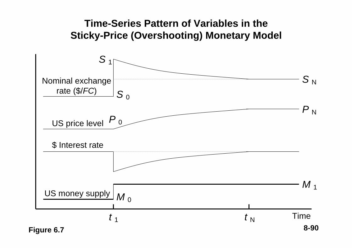
Thirdly, a study by Mark (1995) provides strong evidence that the long-run path of the exchange rate can be accurately gauged from knowledge of the current level of the rate relative to its equilibrium value in a monetary model. The adjustment path corresponds broadly to the overshooting path described in Figure 6.7 - the movement toward the equilibrium should be greater the farther into the future we forecast.


8-90

US price level

$ Interest rate

US money supply

Timet 1 t N

Time-Series Pattern of Variables in the Sticky-Price (Overshooting) Monetary Model

Figure 6.7

Nominal exchange rate ($/FC)

M 0

P 0

S 0

M 1

P N

S 1

S N

8-91

Indeed, Mark’s results conform to this hypothesis. Mark found that on an in-sample basis, his model explains (in terms of R2) between 50-75 percent of the variation in the DM, SFr, and ¥ rates at the three- and four-year horizons. The figures in the next few slides show how the correspondence between the actual exchange rate (indicated by open circles) and the fitted exchange rate (indicated by solid circles) improves as the forecast horizon lengthens to three and four years.


8-92Figure 8.9

Evidence on Long-Horizon Predictability in the DM/$ Rate

8-93Figure 8.9


8-94Figure 8.9


8-95Figure 8.9


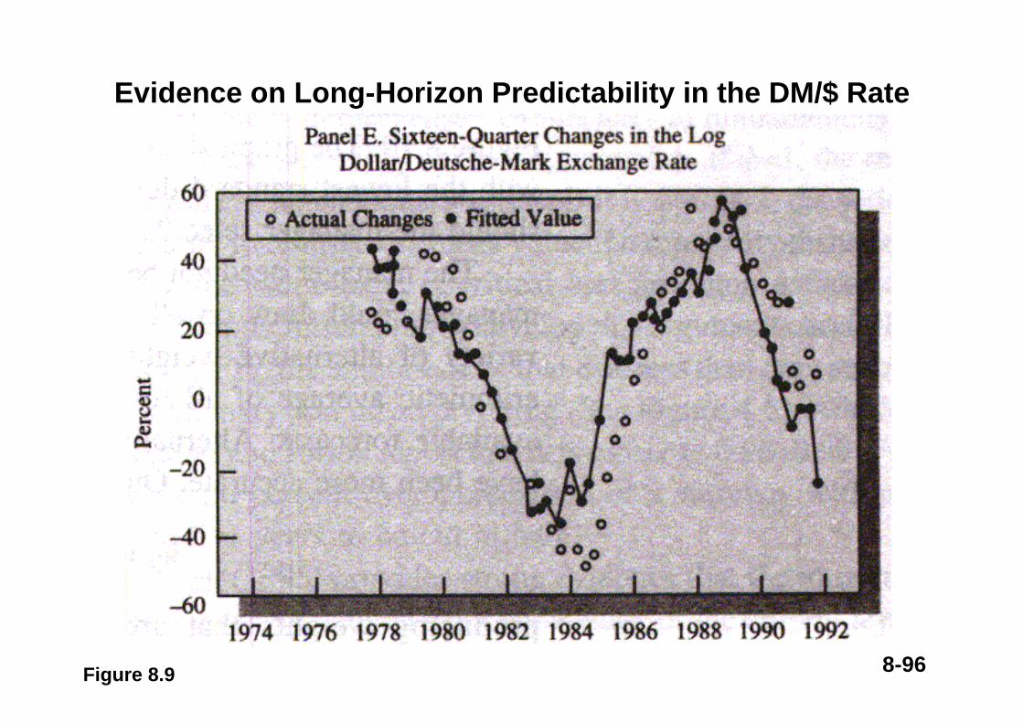
8-96Figure 8.9


8-97

Even in out-of-sample forecasts, Mark’s model significantly outperforms the naïve random walk, reducing the MSE by 20 percent to 59 percent.

Mark, Nelson C. “Exchange Rates and Fundamentals: Evidence on Long-Horizon Predictability and Overshooting.” American Economic Review 85, no. 1 (Mar. 1995), pp. 201-18.


8-98

Overall, these results suggest that at the long-run horizon, there is considerable reason to be optimistic that one can construct a forecast of the real exchange rate that is superior to the random walk.This optimism relies on an assumption of stationarity in real rates which implies a reversion to the mean real rate, or a reversion to the equilibrium exchange rate implied by macroeconomic fundamentals.


8-99

Economic theories usually begin with an internally consistent set of assumptions to develop a stylized model of exchange rate determination. The hope is that the stylized model captures every facet of exchange rate determination, so that the model is both internally consistent and complete.

Forecasting models tend to take a more pragmatic approach. Rather than be doctrinaire, a forecasting model may simply draw on what works from available theoretical models. Composite forecasting illustrates this principle.

Composite Forecasts:Theory and Examples

8-100

A composite forecast brings together the information in alternative forecasting models in an attempt to outperform any of the individual forecasts.In practice, the technique may be successful if individual forecasts reflect complementary elements of information.


8-101

Consider a manager with access to several alternative exchange rate forecast.Assuming that historic data are available on these forecasts, we can compute the mean (μ) and standard deviation (σ) for each series of forecast errors and graph them as in Figure 8.10. The graph shows forecaster 5 with the smallest average error, forecaster 4 with the lowest standard deviation of forecast errors, and so forth. Which forecaster should the manager select?


8-102

Illustrating the Potential Gains from Composite Forecasting over Individual Forecasts

Figure 8.10

Standarddeviation of

forecast errors

Averageforecast

error

S*

S**

μ*

Sc

Sc

• S2

• S4

• S1 • S5

• S6 • S3

Individualforecasts

Locus ofcompositeforecastsComposite forecast

with the smallest σ

8-103

The manager need not be restricted to the use of a single forecast. A variety of alternative weighting systems are possible.The manager could assign a weight of w = 1/n to each of the n available forecasts. Alternatively, greater weight could be assigned to forecasts that have been more accurate by choosing

niw

ii

ii ,...,1 ,1

1

==∑ σ

σ


8-104

The above scheme produce weights that are inversely proportional to each forecast’s standard deviation.

Figure 8.10 suggests that a set of weights (wi) could be chosen to minimize the average forecast error, conditional on the standard deviation.This approach generates a locus SCSC which represents all the possible forecasts that could be formed with alternative weighting schemes.


8-105

The weighting scheme that produces S* appears desirable as it corresponds to the minimum standard deviation forecast.But on an in-sample basis, an alternative forecast can be constructed, S** = S* - μ*, that is both unbiased (average error of zero) and has the minimum standard deviation.


8-106

Linear regression is a simple method to determine the weights in a composite forecast. With n forecasts, the weight on each forecaster can be estimated from the following equation:

tnntttC SwSwSwS ,,22,11,ˆˆˆˆ +⋅⋅⋅++=


8-107

Each regression coefficient is interpreted as the marginal value of information from the ithforecast, conditional on the information in the other n-1 forecasts.Thus, an individual forecast might be fairly accurate, but of little value if it replicates the information in other available forecasts. Alternatively, an individual forecast could be biased or inaccurate, but capture some information that is missing in the other forecasts.


8-108

One drawback of the composite approach is that the weights must be estimated from in-sample data.If the accuracy or the correlation structure of the individual forecasts should change, then the composite forecast need not be superior when applied to out-of-sample data.Still a simple average that assigns a fixed weight (1/n) and draws on no in-sample characteristics (μ, σ, or correlation structure) may produce a superior and more steady forecasting record.


8-109

Assignment from Chapter 8Exercises 1, 2, 3, 4.

http://www.mhhe.com/business/finance/levich2e/

8-110

Chapter 8, Exercise 1

a. The most accurate forecaster had the smallest error of 3.26%.

8-111

The manager need not be restricted to the use of a single forecast. A variety of alternative weighting systems are possible.The manager could assign a weight of w = 1/n to each of the n available forecasts. Alternatively, greater weight could be assigned to forecasts that have been more accurate by choosing

niw

ii

ii ,...,1 ,1

1

==∑ σ

σ



8-112

The above scheme produce weights that are inversely proportional to each forecast’s standard deviation.It has a smaller RMSE and it is less biased since it places greater weights on forecasters that have been more accurate.However, its superiority depends upon the individual forecasters retaining their relative accuracy ratings.



8-113


a. 83.2

b. Yen 82.92 / $

8-114Chapter 8, Exercise 3a

A forecaster’s performance in terms of usefulness can be summarized by the percentage of correct forecasts. We define the percentage of correct forecasts as:

forecasts of number totalforecastscorrect of number

==nrp

A test for forecasting expertise, or market timing:

expertise) or timing (positive expertise) or timing (no

5.0:5.0:

10

>=

pHpH


Consider a series of n independent trials, each resulting in one of two possible outcomes, “success” or “failure.” Let p = P(success occurs at any given trial) and assume that p remains constant from trial to trial. Let the variable X denote the total number of successes in the n trials. Then X is said to have a binomial distribution and

nkppknk

nkXP knk ,... ,1 ,0 )1()!(!

!)( =−−

== −

)1( )( )(2 pnpXVarnpXE

−==

==

σ

μ


dxednpq

npXcPd

c

x

n ∫−

∞→=<

−< 2

2

21π

)(lim

DeMoivre-Laplace Theorem:Let X be a binomial random variable defined on nindependent trials each having success probability p. For any numbers c and d,

According to the binomial distribution, the expected value of p is r/n, and the standard deviation of p is

nnr

nr )1( −

8-117


a. t-value against the null hypothesis = 1.44Is this statistically significant?

b. t-value against the null hypothesis = 2.0Is this statistically significant?



The forecast error made at time t is defined as:

jt

jt

SS tat forecast ahead period-j

+

+

+

+

−=

−=

jt

jtjtt S

SSe ,

ˆ

8-119

n

e

RMSE

n

e

MSE

ii

ii

∑

∑

=

=

2

2

Mean Squared Error:

Root Mean Squared Error:


Chapter 8, Exercise 4a

Answer of 4a: 0.0015, 3.92%; 0.0022, 4.68%

8-120Chapter 8, Exercise 4b

Useful forecasts are those on the “right side of the market” and lead to profitable speculative positions and correct hedging decisions.To measure how often a forecaster’s advice has been on the “right side of the market,” we must have a measure of “the market.” In the absence of a currency risk premium, “right side of the market” implies “right side of the forward rate.”Thus, useful forecasts are those that lead to correct hedging decisions.

Answer of 4b: 83.3%

8-121

The probability of getting 10, 11, or 12 correct forecasts out of 12 (assuming that the forecaster has no expertise) is

%9.14096

112662

!0!12!12

2!1!11!12

2!2!10

!12

121212 ≈++

=++

where 212 represents the number of patterns for tossing a fair coin twelve times.

From part (b), judge if Crystal Ball Associates has done an unusually good job.

Chapter 8, Exercise 4c

8-122

Discuss the accuracy and usefulness of the Crystal Ball Associates forecasts and the forward rate forecasts.

Chapter 8, Exercise 4d

Course web page: week posting... · Chap 8 Chap Chap 3 Chap 7 Scan Read Pages Pages Pages ... Real...

Documents

Transcript of Course web page: week posting... · Chap 8 Chap Chap 3 Chap 7 Scan Read Pages Pages Pages ... Real...