Course in Nonlinear Finite Element Analysis -...
63
Plasticity I Computational Mechanics, AAU, Esbjerg Nonlinear Finite Element Analysis Course in Nonlinear Finite Element Analysis Plasticity I
Transcript of Course in Nonlinear Finite Element Analysis -...

Plasticity IComputational Mechanics, AAU, EsbjergNonlinear Finite Element Analysis
Course in Nonlinear Finite Element Analysis
Plasticity I

Plasticity IComputational Mechanics, AAU, EsbjergNonlinear Finite Element Analysis
Types of structural nonlinearity classifications used in engineering problems
• Geometric nonlinearity• Material nonlinearity:
– time-independent behaviour such as plasticity– time-dependent behaviour such as creep– viscoelastic/viscoplastic behaviour where both
plasticity and creep effects occur simultaneously
• Contact or boundary nonlinearity
Plasticity IComputational Mechanics, AAU, EsbjergNonlinear Finite Element Analysis
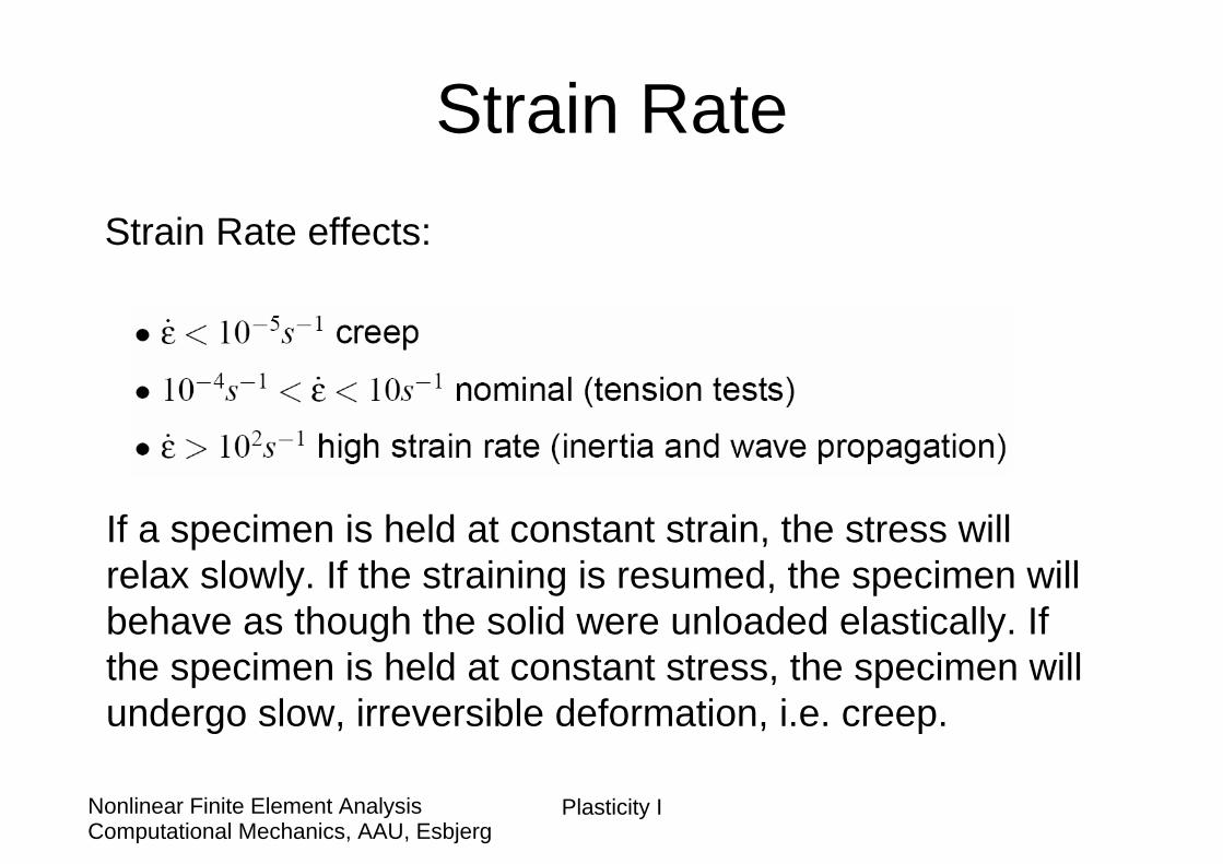
Strain RateStrain Rate effects:
If a specimen is held at constant strain, the stress will relax slowly. If the straining is resumed, the specimen will behave as though the solid were unloaded elastically. If the specimen is held at constant stress, the specimen will undergo slow, irreversible deformation, i.e. creep.
Plasticity IComputational Mechanics, AAU, EsbjergNonlinear Finite Element Analysis
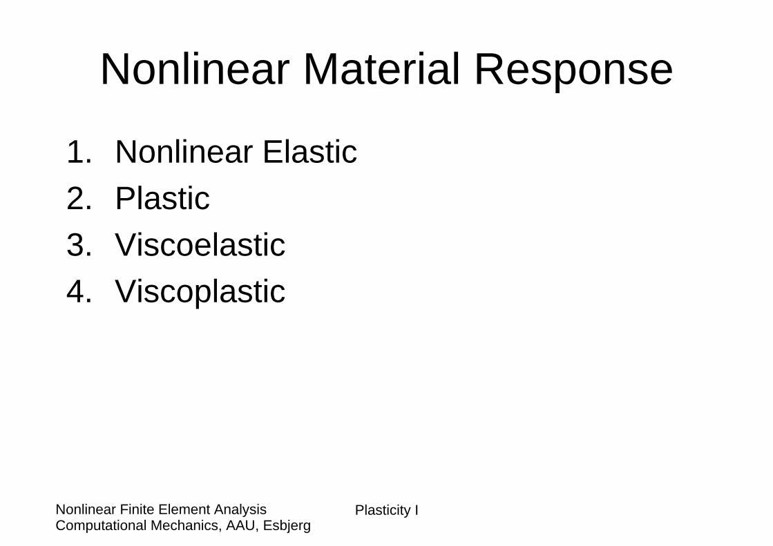
Nonlinear Material Response
1. Nonlinear Elastic2. Plastic3. Viscoelastic4. Viscoplastic
Plasticity IComputational Mechanics, AAU, EsbjergNonlinear Finite Element Analysis
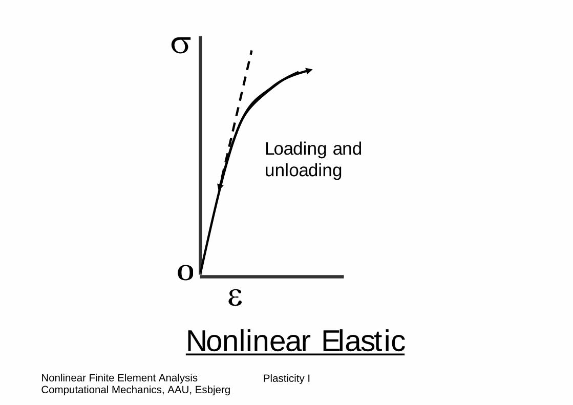
σ
εO
Loading andunloading
Nonlinear Elastic
Plasticity IComputational Mechanics, AAU, EsbjergNonlinear Finite Element Analysis
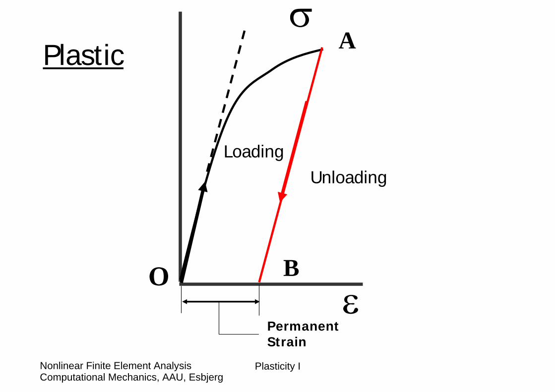
σ
εO
Loading
Plastic A
B
Unloading
PermanentStrain
Plasticity IComputational Mechanics, AAU, EsbjergNonlinear Finite Element Analysis
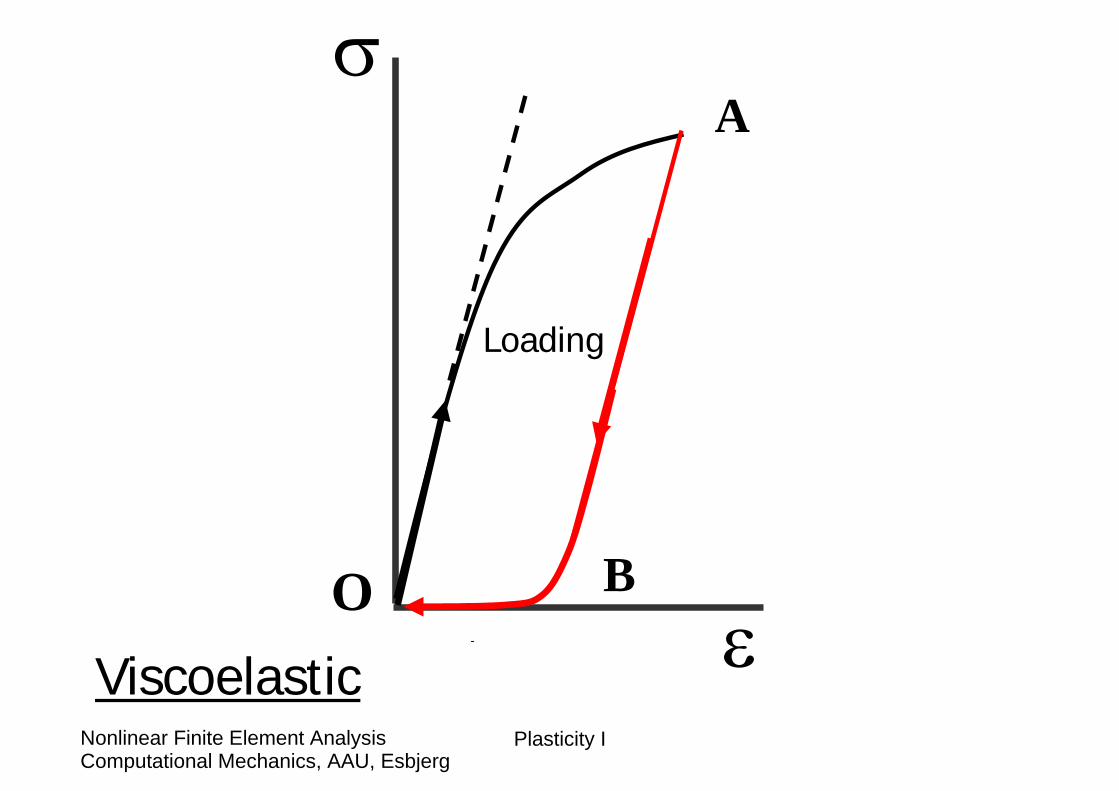
σ
εO
Loading
Viscoelastic
A
B
Plasticity IComputational Mechanics, AAU, EsbjergNonlinear Finite Element Analysis
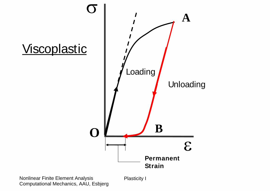
σ
εO
Loading
Viscoplastic
A
B
Unloading
PermanentStrain
Plasticity IComputational Mechanics, AAU, EsbjergNonlinear Finite Element Analysis
Idealized Behavior
1. Elastic-perfectly plastic response2. Elastic-strain hardening response3. Rigid elastic -perfectly plastic response4. Rigid elastic -strain hardening response
Plasticity IComputational Mechanics, AAU, EsbjergNonlinear Finite Element Analysis
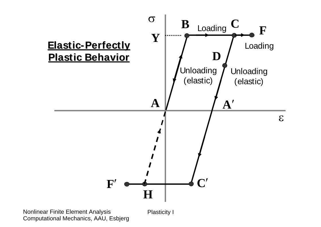
σ
εA A ′
B C F
D
C′F′H
YElasticElastic--Perfectly Perfectly Plastic BehaviorPlastic Behavior
Loading
Loading
Unloading(elastic)
Unloading(elastic)
Plasticity IComputational Mechanics, AAU, EsbjergNonlinear Finite Element Analysis
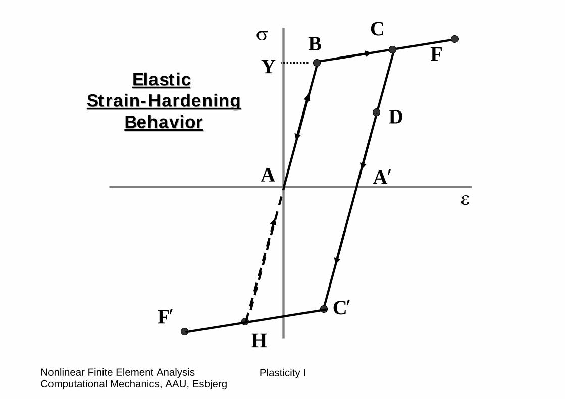
σ
εA A′
BC
F
D
C′F′H
YElastic Elastic
StrainStrain--HardeningHardeningBehaviorBehavior
Plasticity IComputational Mechanics, AAU, EsbjergNonlinear Finite Element Analysis
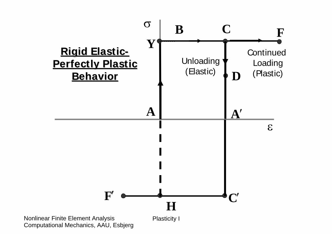
σ
εA A′
B C F
D
C′F′H
YRigid ElasticRigid Elastic--
Perfectly Plastic Perfectly Plastic BehaviorBehavior
Continued Loading(Plastic)
Unloading(Elastic)
Plasticity IComputational Mechanics, AAU, EsbjergNonlinear Finite Element Analysis
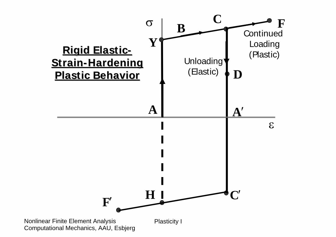
σ
εA A′
BC F
D
C′F′ H
YRigid ElasticRigid Elastic--
StrainStrain--Hardening Hardening Plastic BehaviorPlastic Behavior
Continued Loading(Plastic)
Unloading(Elastic)

Plasticity IComputational Mechanics, AAU, EsbjergNonlinear Finite Element Analysis
Plasticity Theory
• Yield criterion or yield function, i.e. defines the state of stress at which material response changes from elastic to plastic.
• Flow rule, i.e. relates plastic strain increments to stress increments after the onset of initial yielding.
• Hardening rule, i.e. predicts the change in the yield surface due to plastic strains.
Plasticity IComputational Mechanics, AAU, EsbjergNonlinear Finite Element Analysis
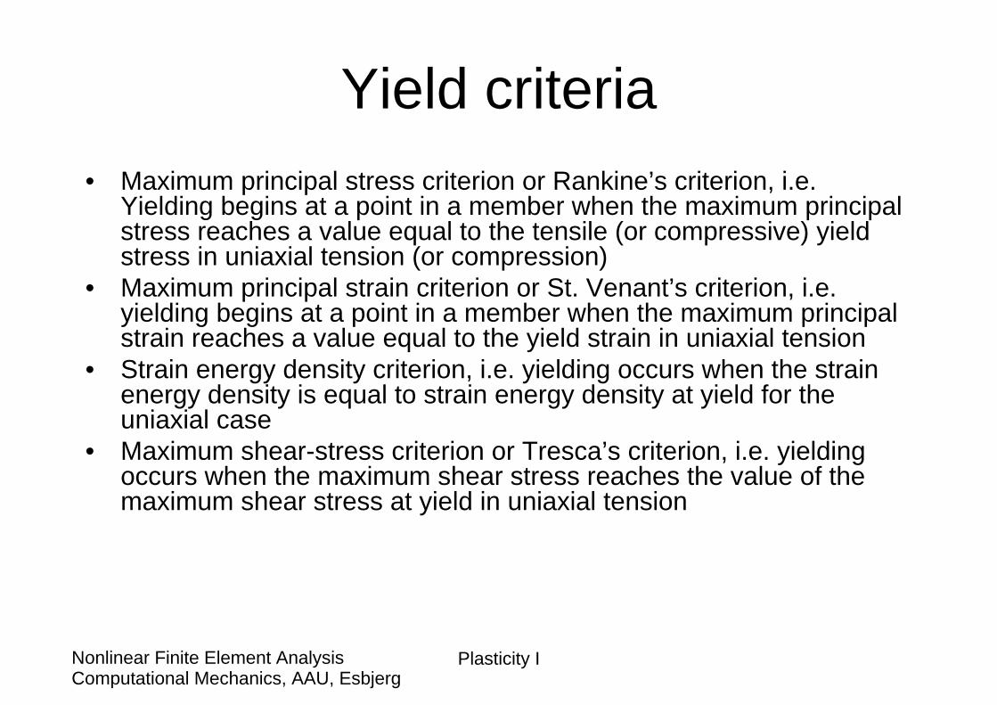
Yield criteria• Maximum principal stress criterion or Rankine’s criterion, i.e.
Yielding begins at a point in a member when the maximum principal stress reaches a value equal to the tensile (or compressive) yield stress in uniaxial tension (or compression)
• Maximum principal strain criterion or St. Venant’s criterion, i.e. yielding begins at a point in a member when the maximum principal strain reaches a value equal to the yield strain in uniaxial tension
• Strain energy density criterion, i.e. yielding occurs when the strain energy density is equal to strain energy density at yield for the uniaxial case
• Maximum shear-stress criterion or Tresca’s criterion, i.e. yielding occurs when the maximum shear stress reaches the value of the maximum shear stress at yield in uniaxial tension
Plasticity IComputational Mechanics, AAU, EsbjergNonlinear Finite Element Analysis
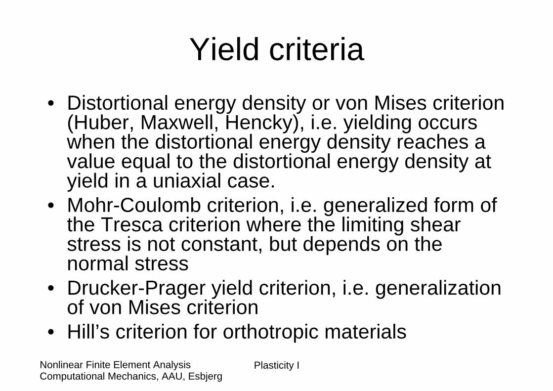
Yield criteria• Distortional energy density or von Mises criterion
(Huber, Maxwell, Hencky), i.e. yielding occurs when the distortional energy density reaches a value equal to the distortional energy density at yield in a uniaxial case.
• Mohr-Coulomb criterion, i.e. generalized form of the Tresca criterion where the limiting shear stress is not constant, but depends on the normal stress
• Drucker-Prager yield criterion, i.e. generalization of von Mises criterion
• Hill’s criterion for orthotropic materials
Plasticity IComputational Mechanics, AAU, EsbjergNonlinear Finite Element Analysis
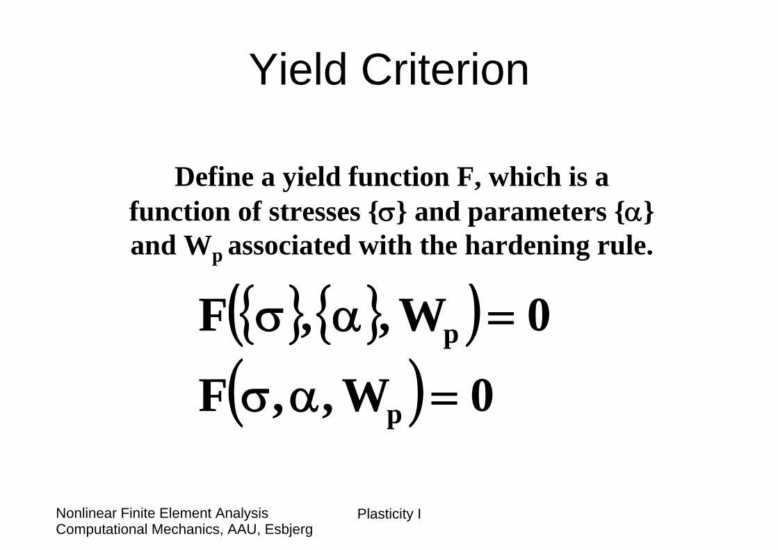
Yield Criterion
Define a yield function F, which is a function of stresses {σ} and parameters {α} and Wp associated with the hardening rule.
{ } { }( )( ) 0W,,F
0W,,F
p
p
=ασ
=ασ
Plasticity IComputational Mechanics, AAU, EsbjergNonlinear Finite Element Analysis
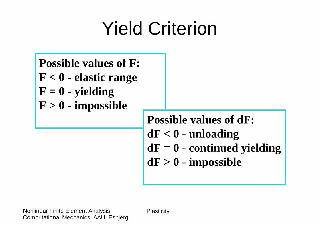
Yield Criterion
Possible values of F:F < 0 - elastic rangeF = 0 - yieldingF > 0 - impossible
Possible values of dF:dF < 0 - unloadingdF = 0 - continued yieldingdF > 0 - impossible
Plasticity IComputational Mechanics, AAU, EsbjergNonlinear Finite Element Analysis
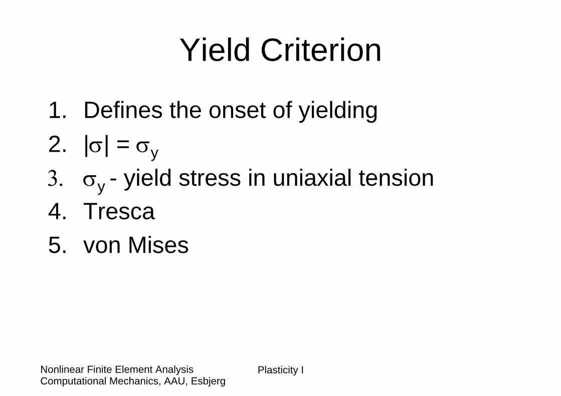
Yield Criterion
1. Defines the onset of yielding2. |σ| = σy
3. σy - yield stress in uniaxial tension4. Tresca5. von Mises
Plasticity IComputational Mechanics, AAU, EsbjergNonlinear Finite Element Analysis
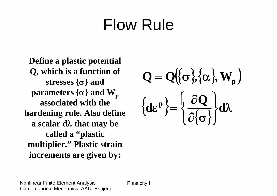
Flow Rule
Define a plastic potential Q, which is a function of
stresses {σ} and parameters {α} and Wp
associated with the hardening rule. Also define
a scalar dλ that may be called a “plastic
multiplier.” Plastic strain increments are given by:
{ } { }( )
{ } { } λ⎭⎬⎫
⎩⎨⎧
σ∂∂
=ε
ασ=
dQd
W,,QQ
p
p
Plasticity IComputational Mechanics, AAU, EsbjergNonlinear Finite Element Analysis
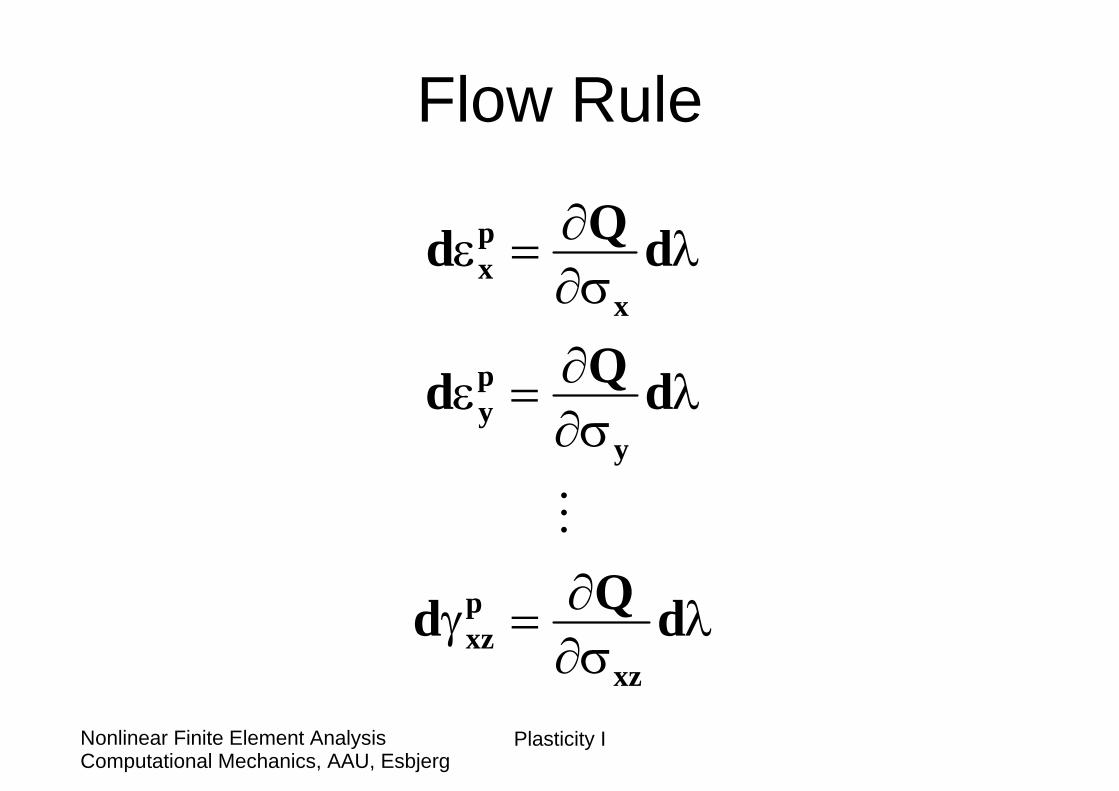
Flow Rule
λσ∂∂=γ
λσ∂∂=ε
λσ∂∂=ε
dQd
dQd
dQd
xz
pxz
y
py
x
px
M
Plasticity IComputational Mechanics, AAU, EsbjergNonlinear Finite Element Analysis
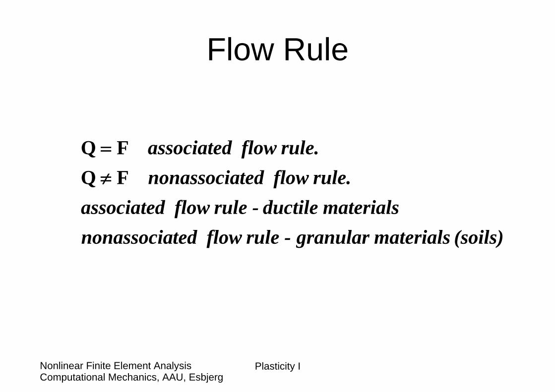
Flow Rule
(soils) materials granular rule - flow tednonassociamaterialsductile rule - flow associated
rule. flow tednonassociarule. flow associated
FQFQ
≠=
Plasticity IComputational Mechanics, AAU, EsbjergNonlinear Finite Element Analysis
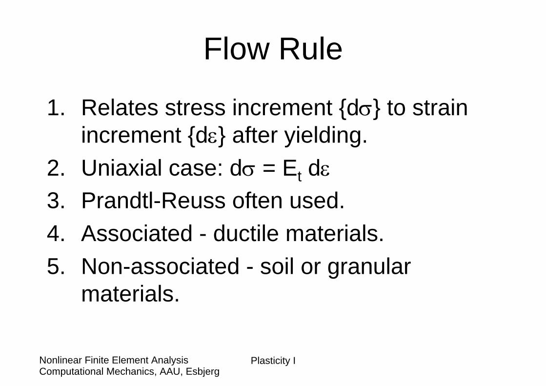
Flow Rule
1. Relates stress increment {dσ} to strain increment {dε} after yielding.
2. Uniaxial case: dσ = Et dε3. Prandtl-Reuss often used.4. Associated - ductile materials.5. Non-associated - soil or granular
materials.
Plasticity IComputational Mechanics, AAU, EsbjergNonlinear Finite Element Analysis
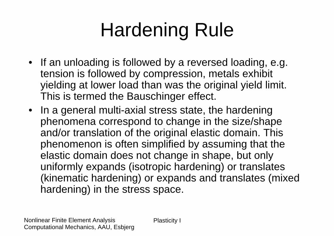
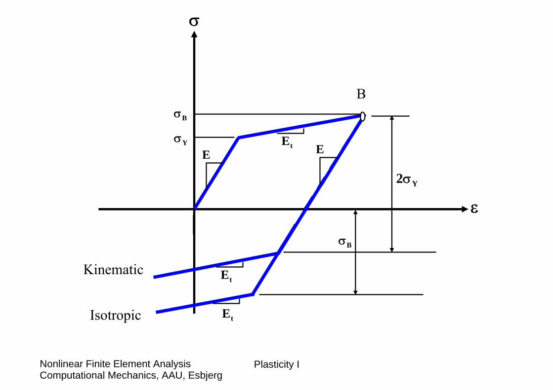
Hardening Rule• If an unloading is followed by a reversed loading, e.g.
tension is followed by compression, metals exhibit yielding at lower load than was the original yield limit. This is termed the Bauschinger effect.
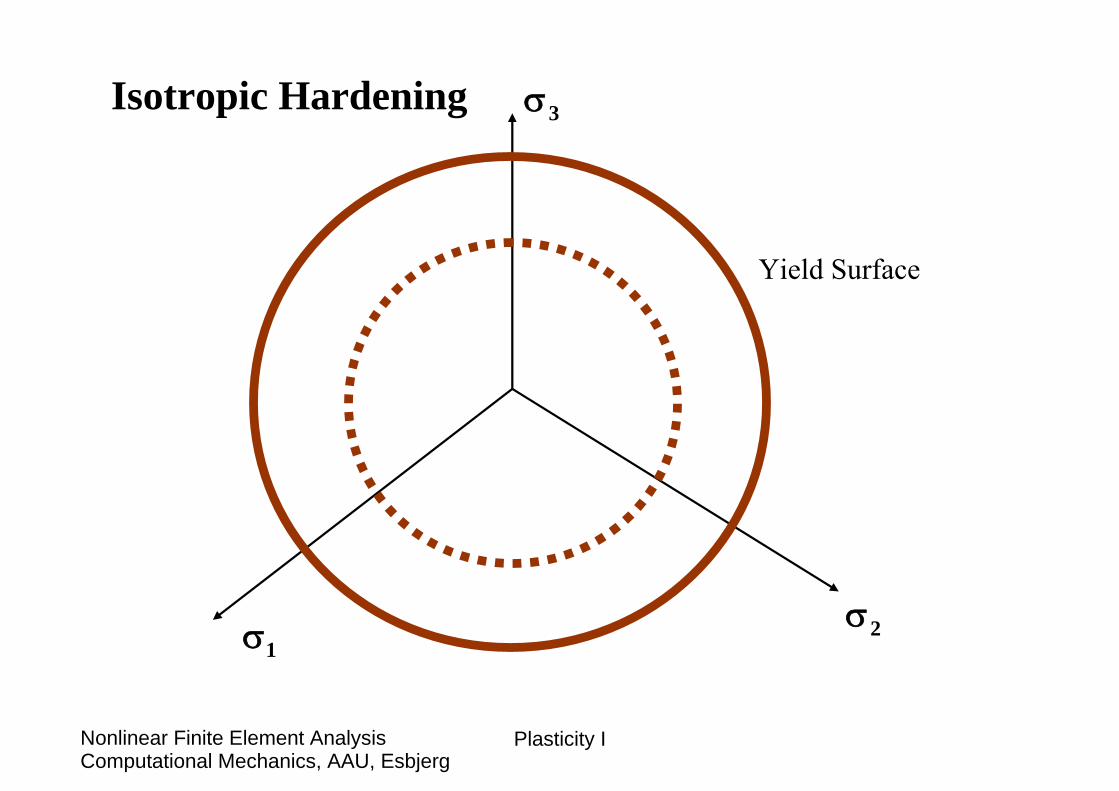
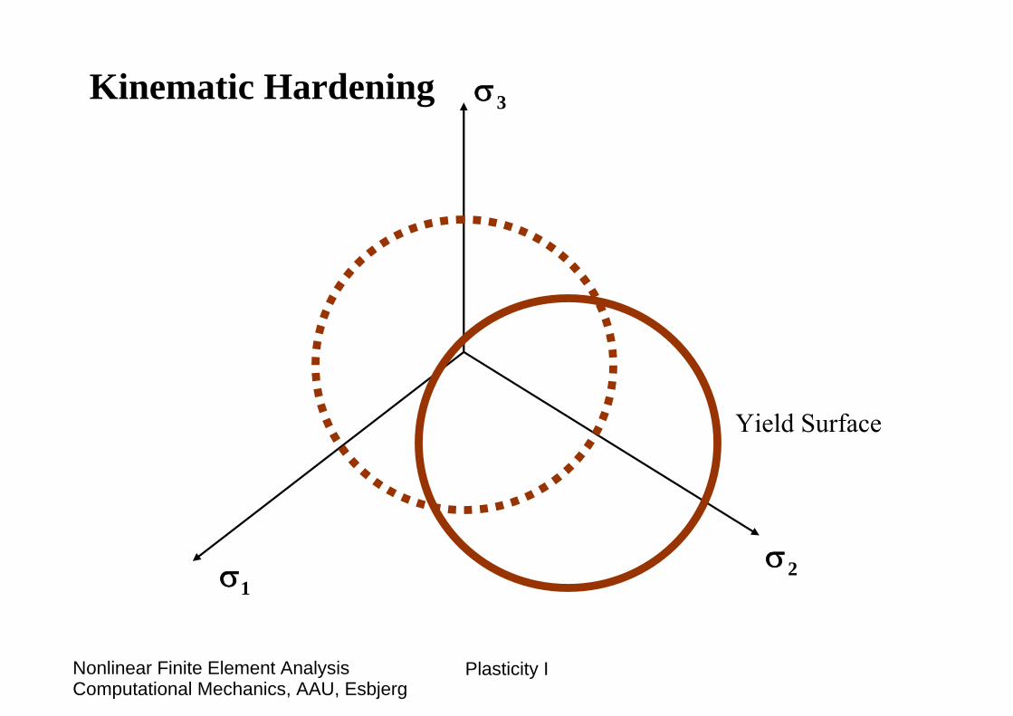
• In a general multi-axial stress state, the hardening phenomena correspond to change in the size/shape and/or translation of the original elastic domain. This phenomenon is often simplified by assuming that the elastic domain does not change in shape, but only uniformly expands (isotropic hardening) or translates (kinematic hardening) or expands and translates (mixed hardening) in the stress space.
Plasticity IComputational Mechanics, AAU, EsbjergNonlinear Finite Element Analysis
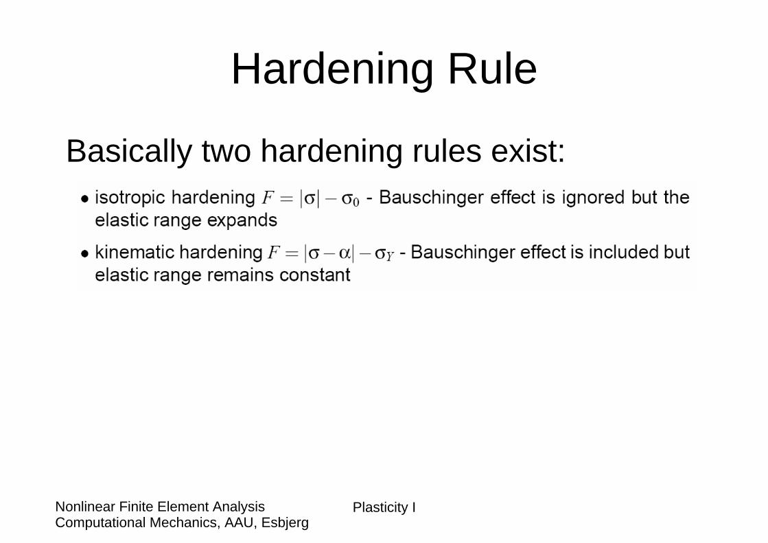
Hardening Rule
Basically two hardening rules exist:
Plasticity IComputational Mechanics, AAU, EsbjergNonlinear Finite Element Analysis
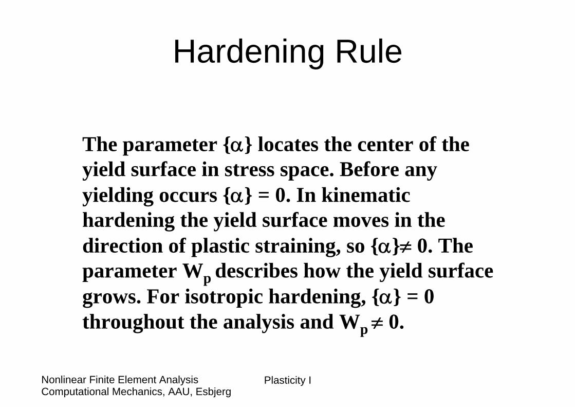
Hardening Rule
The parameter {α} locates the center of the yield surface in stress space. Before any yielding occurs {α} = 0. In kinematic hardening the yield surface moves in the direction of plastic straining, so {α}≠ 0. The parameter Wp describes how the yield surface grows. For isotropic hardening, {α} = 0 throughout the analysis and Wp ≠ 0.
Plasticity IComputational Mechanics, AAU, EsbjergNonlinear Finite Element Analysis
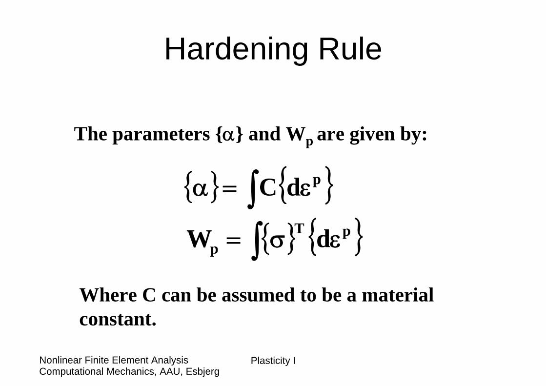
Hardening Rule
The parameters {α} and Wp are given by:
{ } { }{ } { }∫∫
εσ=
ε=α
pTp
p
dW
dC
Where C can be assumed to be a material constant.
Plasticity IComputational Mechanics, AAU, EsbjergNonlinear Finite Element Analysis
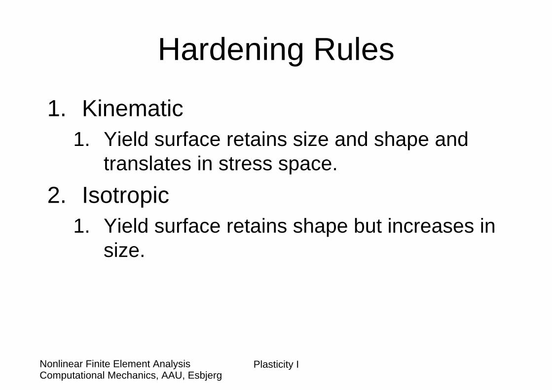
Hardening Rules
1. Kinematic1. Yield surface retains size and shape and
translates in stress space.2. Isotropic
1. Yield surface retains shape but increases in size.
Plasticity IComputational Mechanics, AAU, EsbjergNonlinear Finite Element Analysis
ε
σ
B
YσE E
Y2σ
Bσ
Bσ
tE
tE
tE
Kinematic
Isotropic
Plasticity IComputational Mechanics, AAU, EsbjergNonlinear Finite Element Analysis
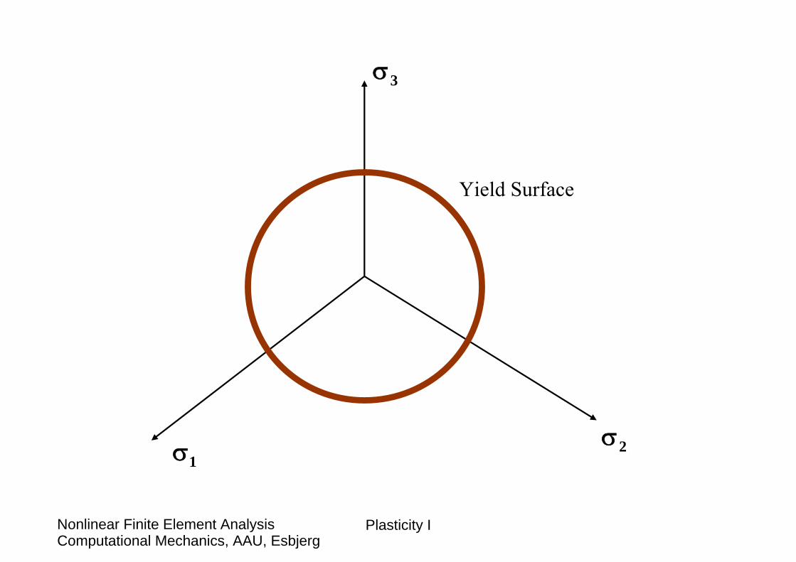
1σ
3σ
2σ
Yield Surface
Plasticity IComputational Mechanics, AAU, EsbjergNonlinear Finite Element Analysis
1σ
3σ
2σ
Yield Surface
Isotropic Hardening
Plasticity IComputational Mechanics, AAU, EsbjergNonlinear Finite Element Analysis
1σ
3σ
2σ
Yield Surface
Kinematic Hardening
Plasticity IComputational Mechanics, AAU, EsbjergNonlinear Finite Element Analysis
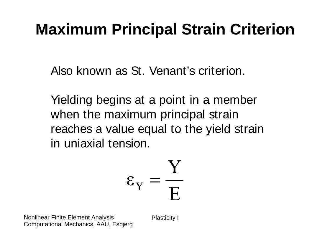
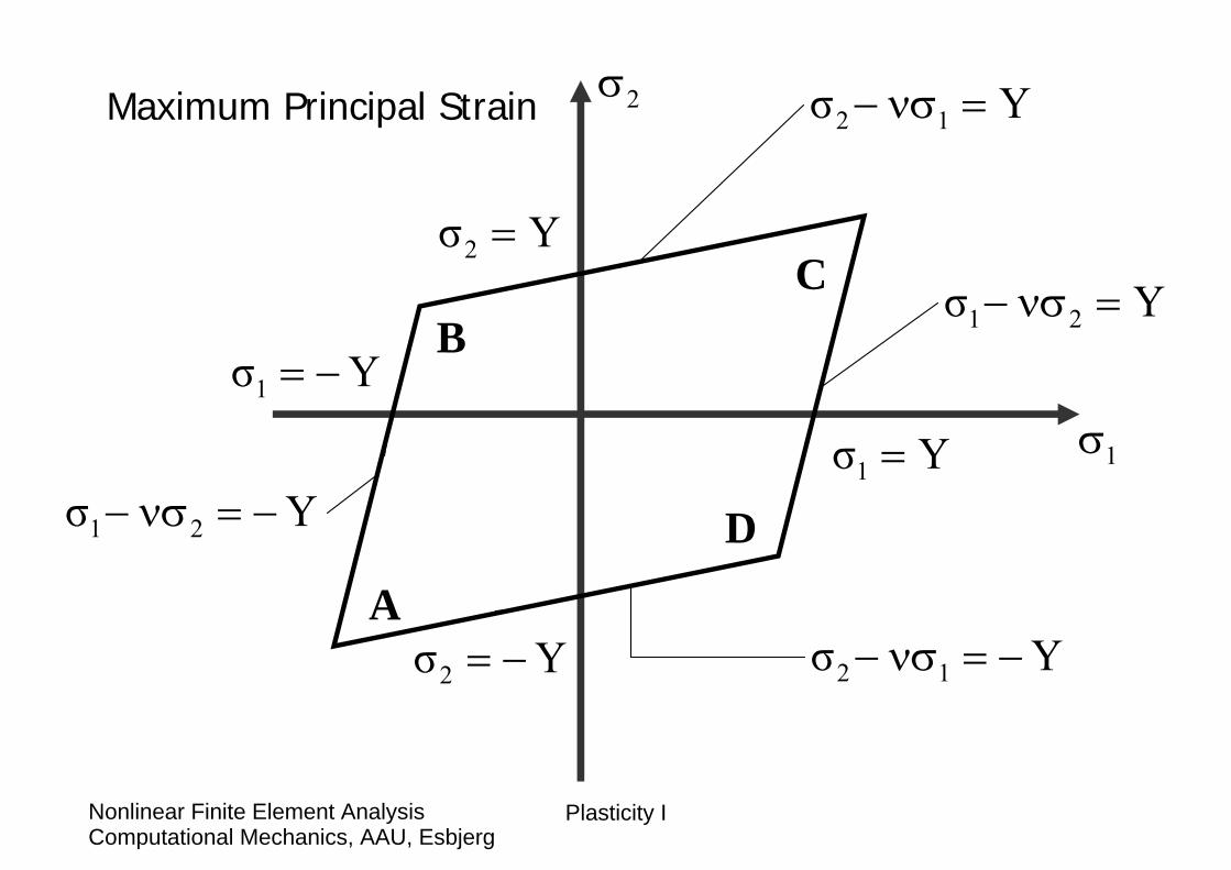
Maximum Principal Strain Criterion
Also known as St. Venant’s criterion.
Yielding begins at a point in a member when the maximum principal strain reaches a value equal to the yield strain in uniaxial tension.
EYεY =
Plasticity IComputational Mechanics, AAU, EsbjergNonlinear Finite Element Analysis
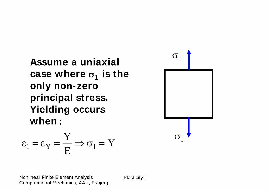
1σ
1σ
Assume a uniaxial case where σ1 is the only non-zero principal stress. Yielding occurs when :
1 Y 1Y YE
ε = ε = ⇒ σ =
Plasticity IComputational Mechanics, AAU, EsbjergNonlinear Finite Element Analysis
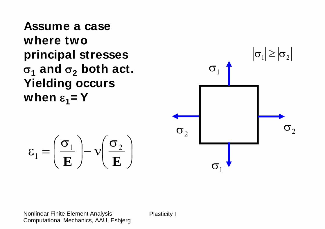
1σ
1σ
2σ2σ
Assume a case where two principal stresses σ1 and σ2 both act. Yielding occurs when ε1=Y
21 σ≥σ
⎟⎠⎞
⎜⎝⎛ σν−⎟
⎠⎞
⎜⎝⎛ σ=ε
EE21
1
Plasticity IComputational Mechanics, AAU, EsbjergNonlinear Finite Element Analysis
1σ
1σ
2σ2σ
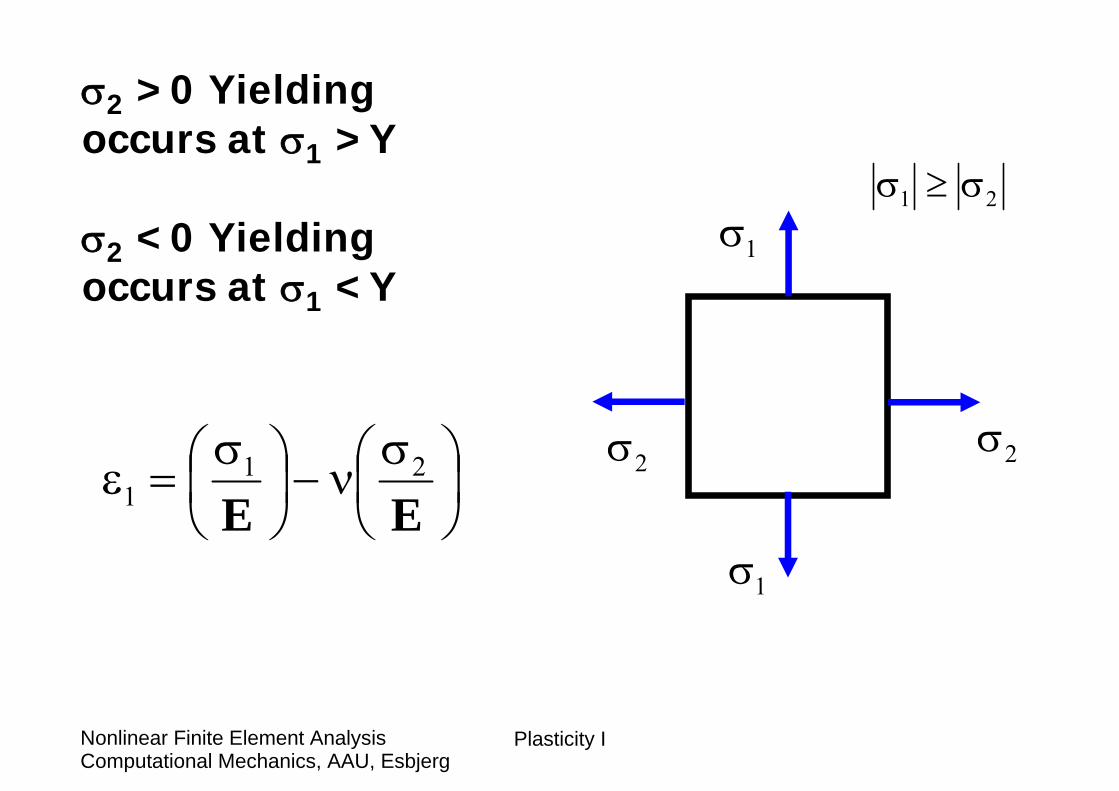
σ2 >0 Yielding occurs at σ1 >Y
σ2 <0 Yielding occurs at σ1 <Y
21 σ≥σ
⎟⎠⎞
⎜⎝⎛ σν−⎟
⎠⎞
⎜⎝⎛ σ=ε
EE21
1
Plasticity IComputational Mechanics, AAU, EsbjergNonlinear Finite Element Analysis
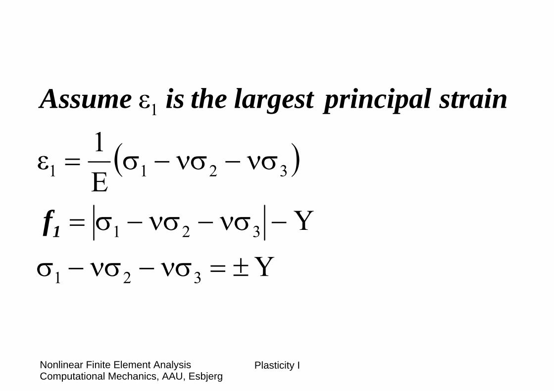
( )
YY
E1ε
ε
321
321
3211
1
±=νσ−νσ−σ
−νσ−νσ−σ=
νσ−νσ−σ=
1f
strain principal largestthe is Assume
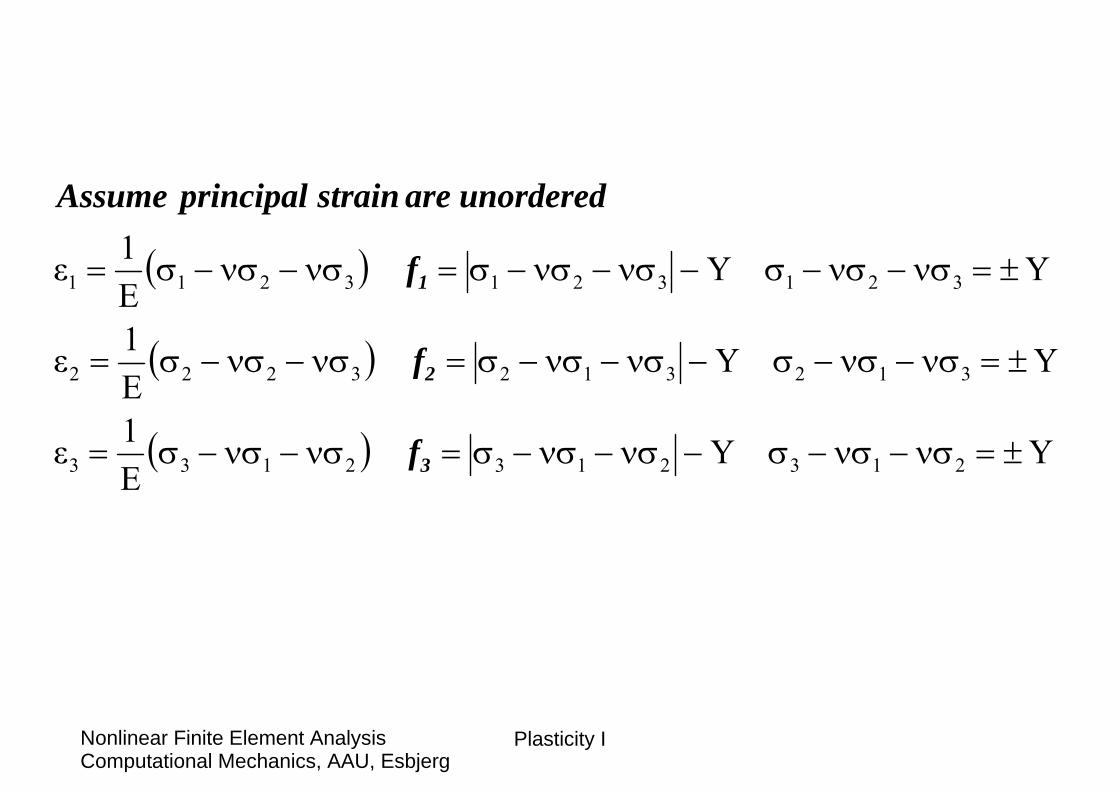
Plasticity IComputational Mechanics, AAU, EsbjergNonlinear Finite Element Analysis
( )
( )
( ) YYE1ε
YYE1ε
YYE1ε
2132132133
3123123222
3213213211
±=νσ−νσ−σ−νσ−νσ−σ=νσ−νσ−σ=
±=νσ−νσ−σ−νσ−νσ−σ=νσ−νσ−σ=
±=νσ−νσ−σ−νσ−νσ−σ=νσ−νσ−σ=
3
2
1
f
f
f
unorderedare strain principalAssume
Plasticity IComputational Mechanics, AAU, EsbjergNonlinear Finite Element Analysis
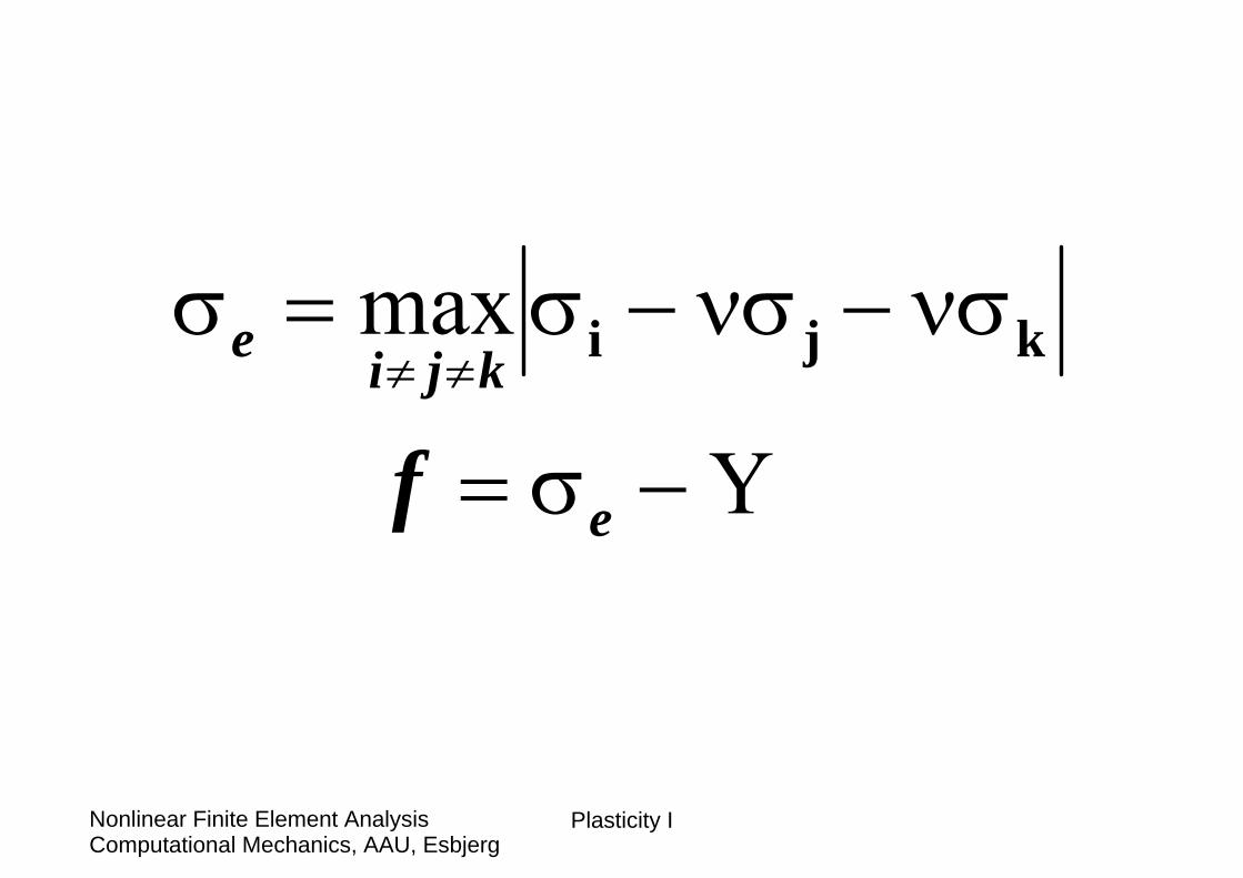
Y
max
−σ=
νσ−νσ−σ=σ≠≠
e
kjie
f
kji
Plasticity IComputational Mechanics, AAU, EsbjergNonlinear Finite Element Analysis
1σ
2σ
Yσ1 =
Yσ1 −=
Yσ2 =
Yσ2 −=
Yσ 12 =νσ−
Yσ 21 =νσ−
Yσ 21 −=νσ−
Yσ 12 −=νσ−A
BC
D
Maximum Principal Strain
Plasticity IComputational Mechanics, AAU, EsbjergNonlinear Finite Element Analysis
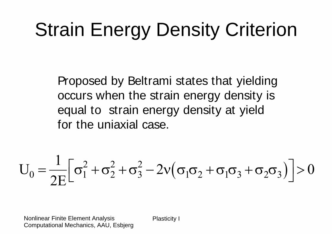
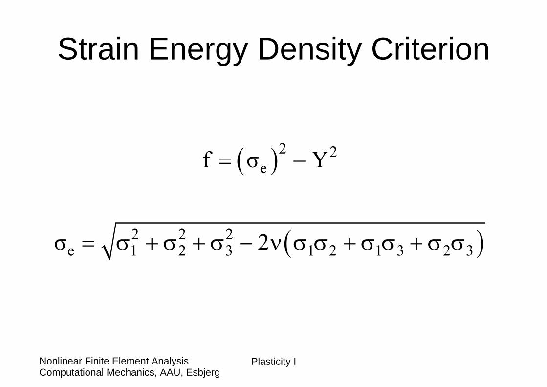
Strain Energy Density Criterion
Proposed by Beltrami states that yielding occurs when the strain energy density is equal to strain energy density at yield for the uniaxial case.
( )2 2 20 1 2 3 1 2 1 3 2 3
1U 2 02E
⎡ ⎤= σ +σ +σ − ν σ σ +σ σ +σ σ >⎣ ⎦
Plasticity IComputational Mechanics, AAU, EsbjergNonlinear Finite Element Analysis
Strain Energy Density Criterion
( )[ ]
[ ]E2
YE2
1U
0Y
2E2
1U
2210
321
32312123
22
210
=σ=
=σ=σ=σ
σσ+σσ+σσν−σ+σ+σ=
:case Uniaxial
Plasticity IComputational Mechanics, AAU, EsbjergNonlinear Finite Element Analysis
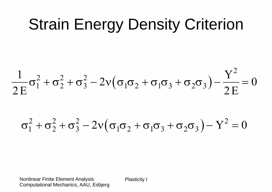
Strain Energy Density Criterion
( )
( )
22 2 21 2 3 1 2 1 3 2 3
2 2 2 21 2 3 1 2 1 3 2 3
1 Y2 02 E 2 E
2 Y 0
σ + σ + σ − ν σ σ + σ σ + σ σ − =
σ + σ + σ − ν σ σ + σ σ + σ σ − =
Plasticity IComputational Mechanics, AAU, EsbjergNonlinear Finite Element Analysis
Strain Energy Density Criterion
( )
( )
2 2e
2 2 2e 1 2 3 1 2 1 3 2 3
f σ Y
σ 2
= −
= σ + σ + σ − ν σ σ + σ σ + σ σ
Plasticity IComputational Mechanics, AAU, EsbjergNonlinear Finite Element Analysis
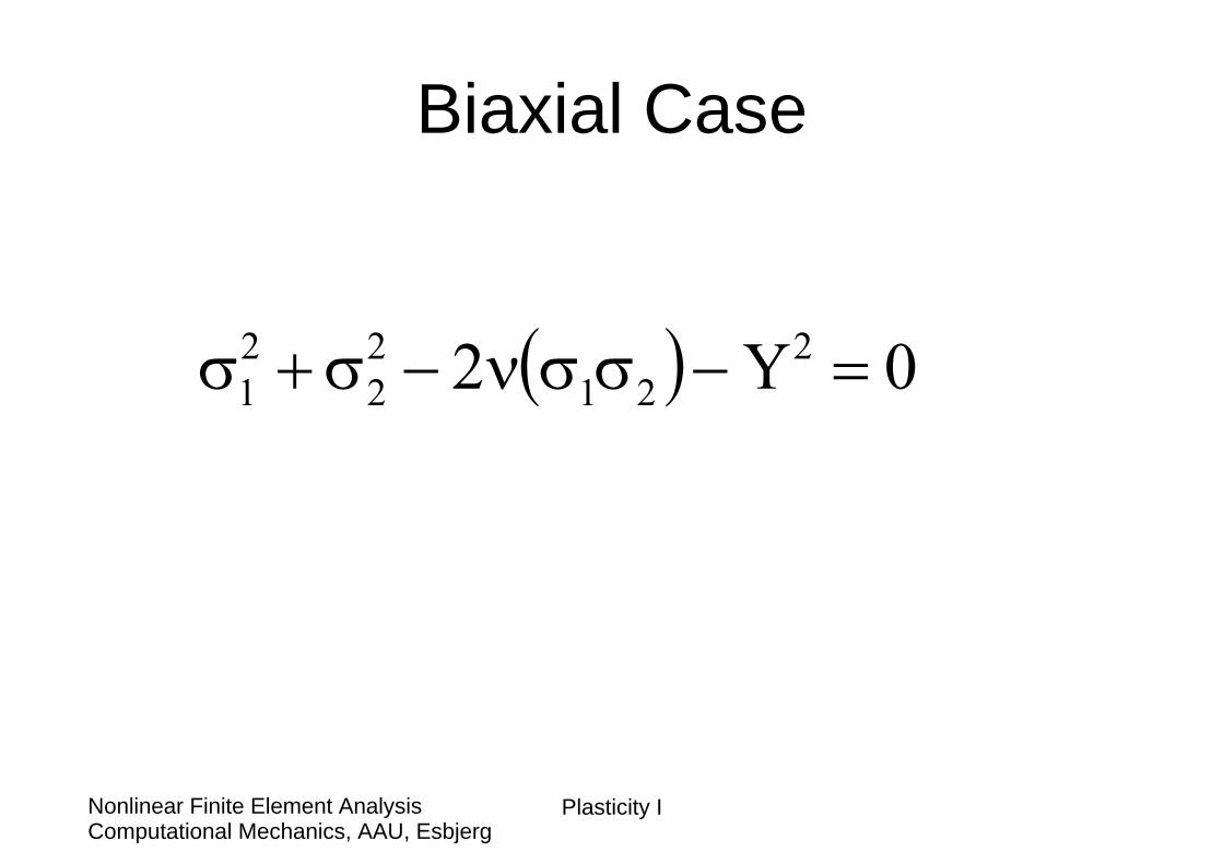
Biaxial Case
( ) 0Y2 221
22
21 =−σσν−σ+σ
Plasticity IComputational Mechanics, AAU, EsbjergNonlinear Finite Element Analysis
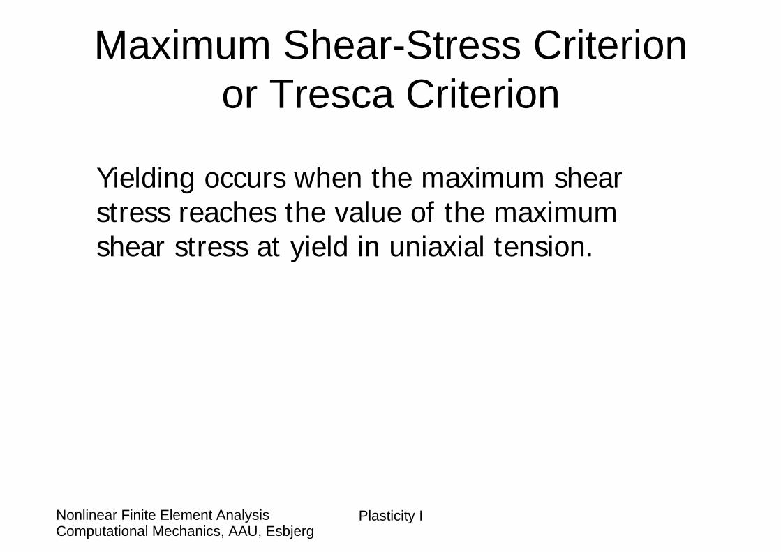
Maximum Shear-Stress Criterionor Tresca Criterion
Yielding occurs when the maximum shear stress reaches the value of the maximum shear stress at yield in uniaxial tension.
Plasticity IComputational Mechanics, AAU, EsbjergNonlinear Finite Element Analysis
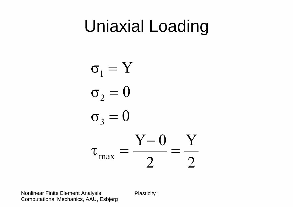
Uniaxial Loading
2Y
20Y
0σ0σYσ
max
3
2
1
=−
=τ
===
Plasticity IComputational Mechanics, AAU, EsbjergNonlinear Finite Element Analysis
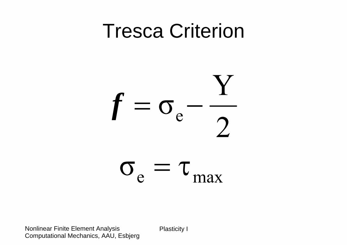
Tresca Criterion
maxe
e
σ2Yσ
τ=
−=f
Plasticity IComputational Mechanics, AAU, EsbjergNonlinear Finite Element Analysis
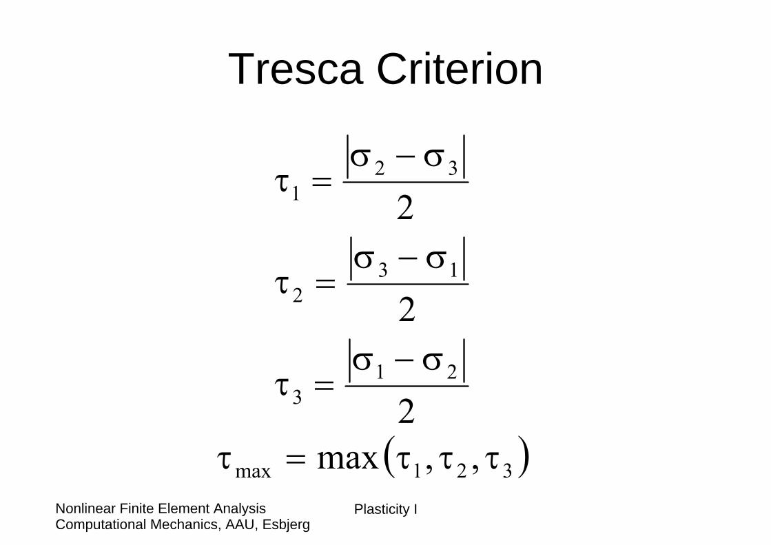
Tresca Criterion
( )321max
213
132
321
,,max2
2
2
τττ=τ
σ−σ=τ
σ−σ=τ
σ−σ=τ
Plasticity IComputational Mechanics, AAU, EsbjergNonlinear Finite Element Analysis
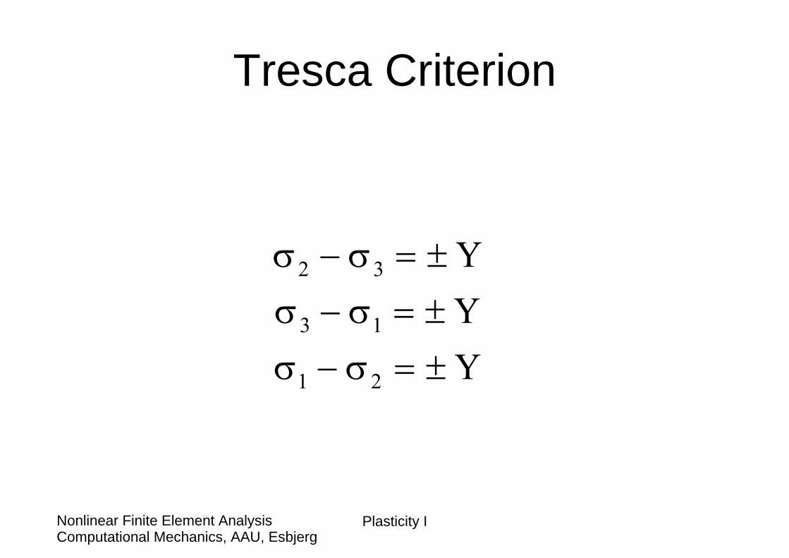
Tresca Criterion
YYY
21
13
32
±=σ−σ±=σ−σ±=σ−σ
Plasticity IComputational Mechanics, AAU, EsbjergNonlinear Finite Element Analysis
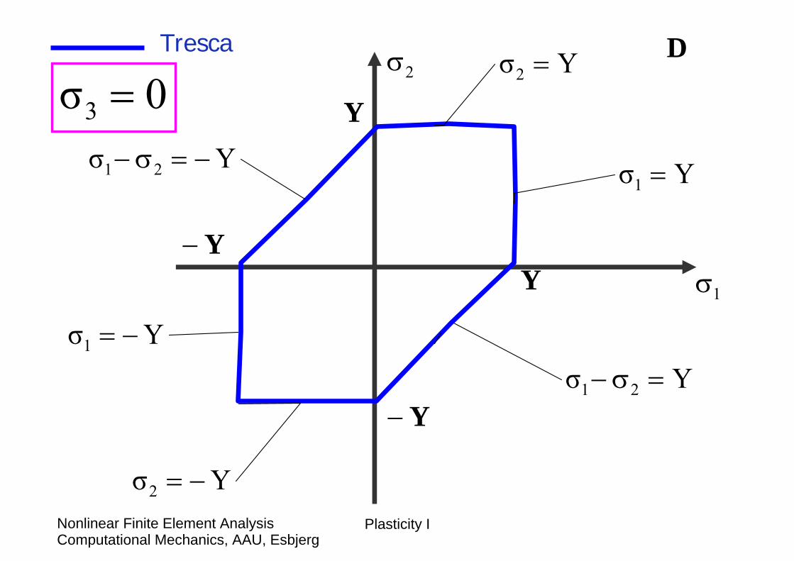
1σ
2σ
Yσ1 =
Yσ1 −=
Yσ2 =
Yσ2 −=
Y
D
Yσ 21 =σ−
Y
Y−
Y−
Yσ 21 −=σ−
Tresca
0σ3 =
Plasticity IComputational Mechanics, AAU, EsbjergNonlinear Finite Element Analysis
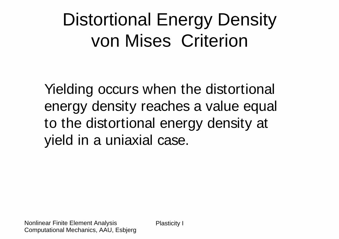
Distortional Energy Density von Mises Criterion
Yielding occurs when the distortional energy density reaches a value equal to the distortional energy density at yield in a uniaxial case.
Plasticity IComputational Mechanics, AAU, EsbjergNonlinear Finite Element Analysis
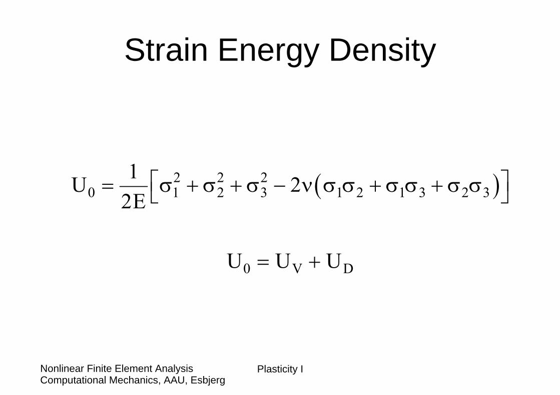
Strain Energy Density
( )2 2 20 1 2 3 1 2 1 3 2 3
0 V D
1U 22E
U U U
⎡ ⎤= σ + σ + σ − ν σ σ + σ σ + σ σ⎣ ⎦
= +
Plasticity IComputational Mechanics, AAU, EsbjergNonlinear Finite Element Analysis
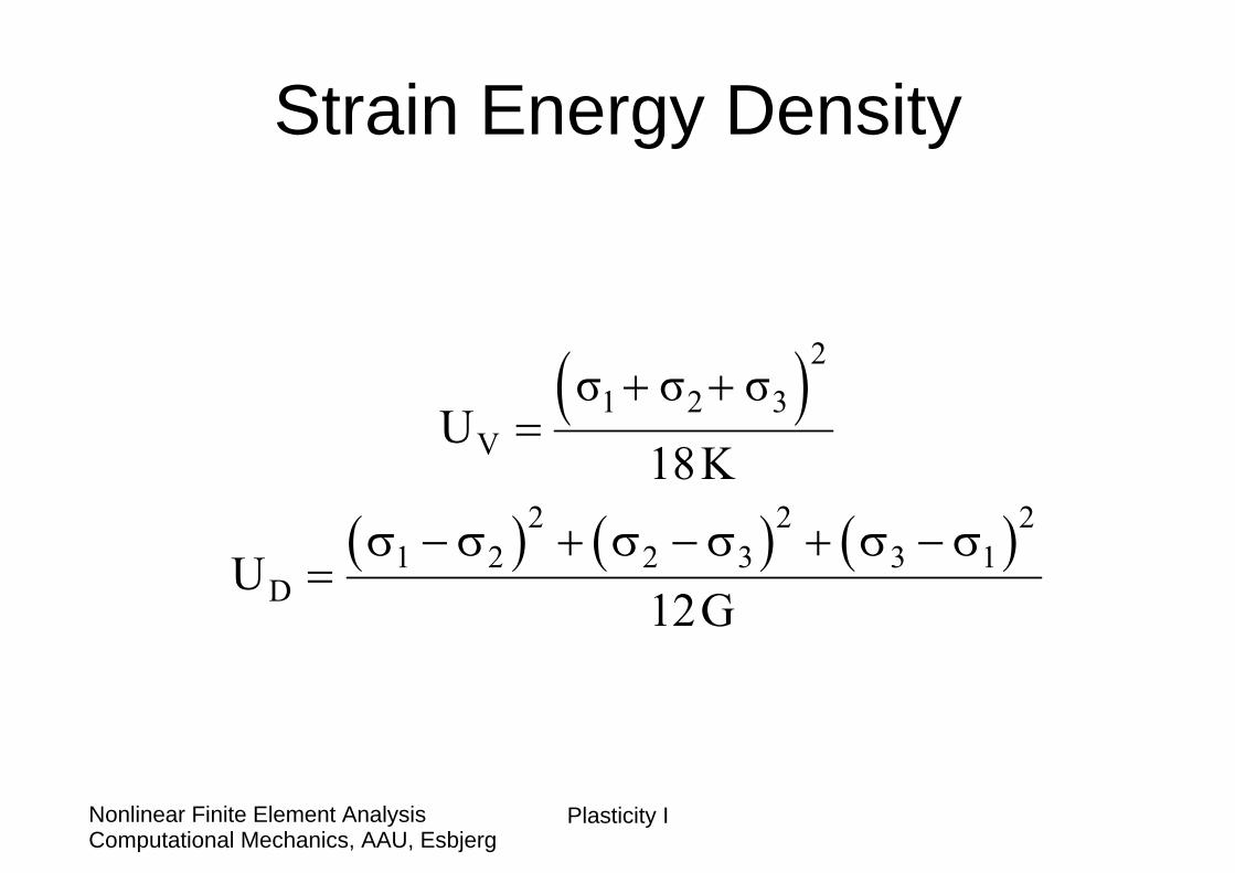
Strain Energy Density
( )
( ) ( ) ( )
21 2 3
V
2 2 21 2 2 3 3 1
D
σ σ σU
18K
U12G
+ +=
σ − σ + σ − σ + σ − σ=
Plasticity IComputational Mechanics, AAU, EsbjergNonlinear Finite Element Analysis
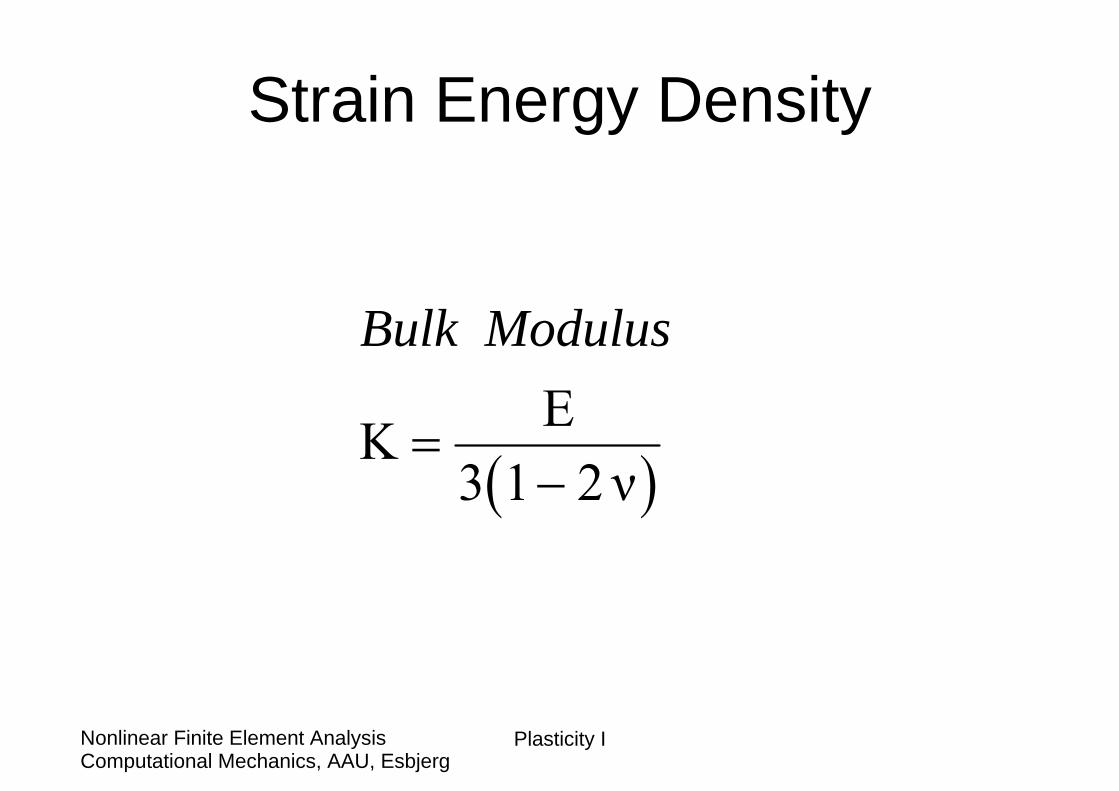
Strain Energy Density
( )EK
3 1 2 ν
Bulk Modulus
=−
Plasticity IComputational Mechanics, AAU, EsbjergNonlinear Finite Element Analysis
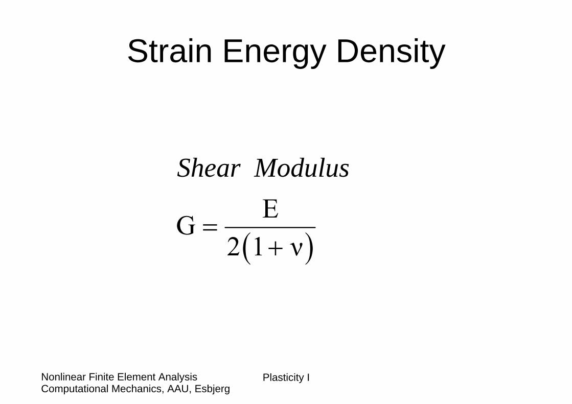
Strain Energy Density
( )EG
2 1 ν
Shear Modulus
=+
Plasticity IComputational Mechanics, AAU, EsbjergNonlinear Finite Element Analysis
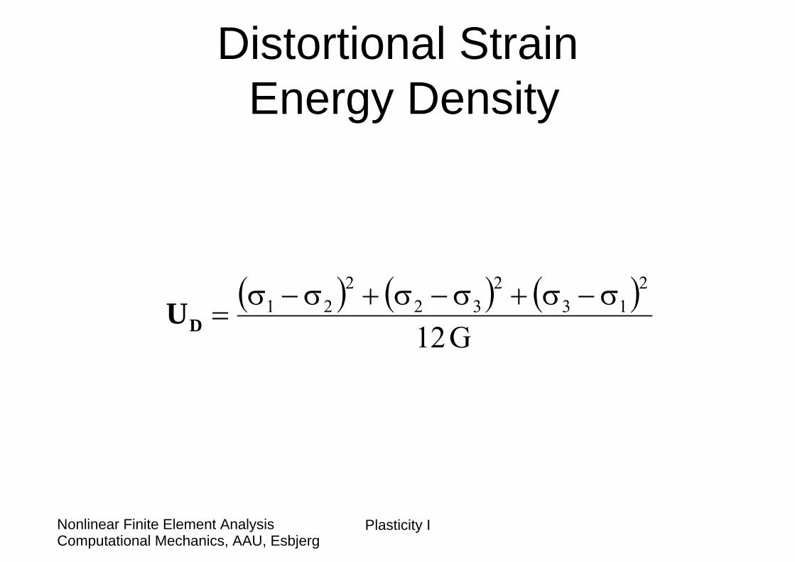
Distortional StrainEnergy Density
( ) ( ) ( )G12
213
232
221 σ−σ+σ−σ+σ−σ
=DU
Plasticity IComputational Mechanics, AAU, EsbjergNonlinear Finite Element Analysis
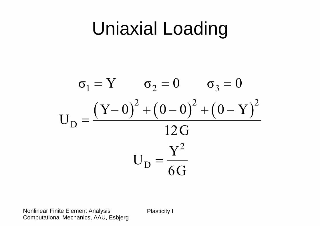
Uniaxial Loading
( ) ( ) ( )1 2 3
2 2 2
D
2
D
σ Y σ 0 σ 0
Y 0 0 0 0 YU
12GYU6G
= = =
− + − + −=
=
Plasticity IComputational Mechanics, AAU, EsbjergNonlinear Finite Element Analysis
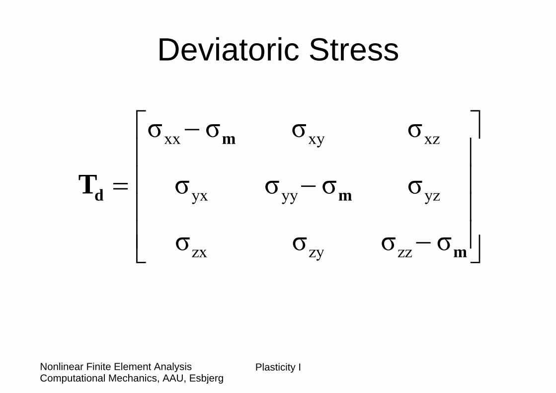
Deviatoric Stress
⎥⎥⎥⎥
⎦
⎤
⎢⎢⎢⎢
⎣
⎡
−
−
−
=
m
m
m
dT
σσσσ
σσσσ
σσσσ
zzzyzx
yzyyyx
xzxyxx
Plasticity IComputational Mechanics, AAU, EsbjergNonlinear Finite Element Analysis
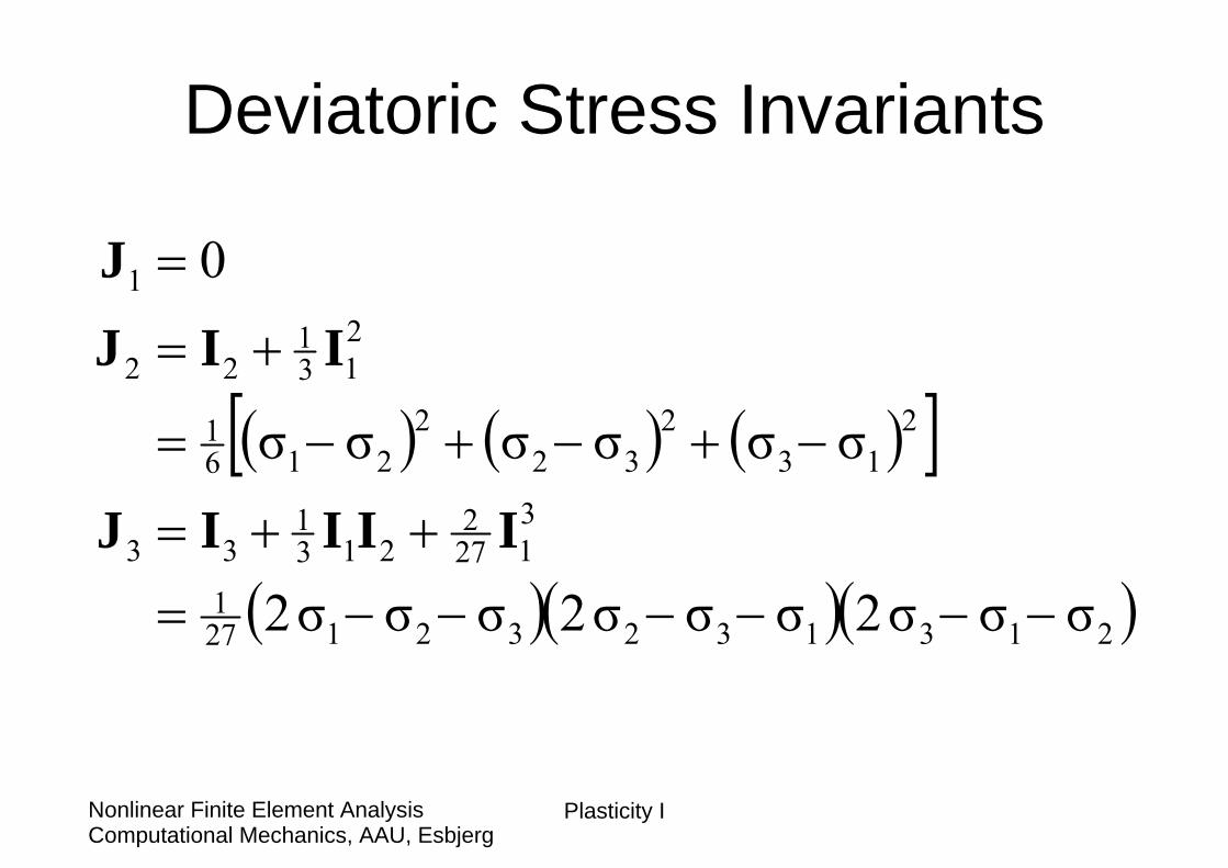
( ) ( ) ( )[ ]
( )( )( )213132321271
3127
2213
133
213
232
2216
1
213
122
1
σσσ2σσσ2σσσ2
σσσσσσ
0
−−−−−−=
++=
−+−+−=
+=
=
IIIIJ
IIJ
J
Deviatoric Stress Invariants
Plasticity IComputational Mechanics, AAU, EsbjergNonlinear Finite Element Analysis
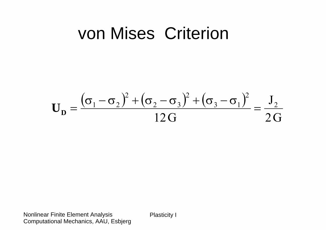
von Mises Criterion
( ) ( ) ( )G2
JG12
22
132
322
21 =σ−σ+σ−σ+σ−σ
=DU
Plasticity IComputational Mechanics, AAU, EsbjergNonlinear Finite Element Analysis
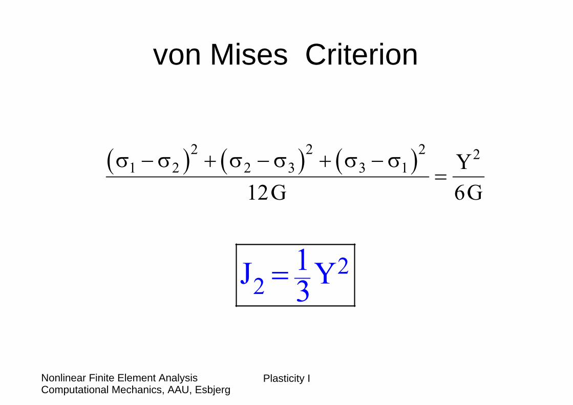
von Mises Criterion
( ) ( ) ( )2 2 2 21 2 2 3 3 1 Y
12G 6G
22
1J Y3
σ − σ + σ − σ + σ − σ=
=
Plasticity IComputational Mechanics, AAU, EsbjergNonlinear Finite Element Analysis
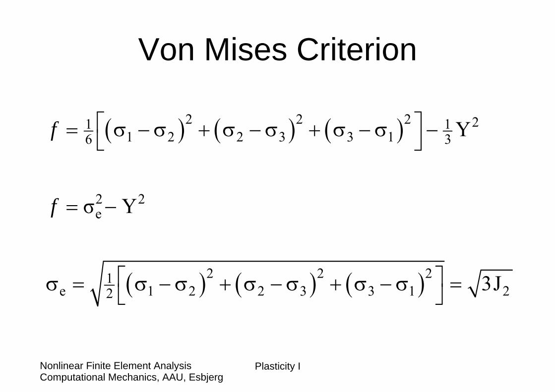
Von Mises Criterion
( ) ( ) ( )
( ) ( ) ( )
2 2 2 21 11 2 2 3 3 16 3
2 2e
2 2 21e 1 2 2 3 3 1 22
Y
σ Y
3J
f
f
⎡ ⎤= σ − σ + σ − σ + σ − σ −⎣ ⎦
= −
⎡ ⎤σ = σ − σ + σ − σ + σ − σ =⎣ ⎦

![Introduction - Aalborg Universitethomes.civil.aau.dk/shl/ansysc/fem-nonlinear-introduction.pdf · • [ANSYS] ANSYS 10.0 Documentation (installed with ANSYS): – Basic Analysis Procedures](https://static.fdocuments.net/doc/165x107/608b42231337ee1469269f09/introduction-aalborg-a-ansys-ansys-100-documentation-installed-with-ansys.jpg)