Course in Nonlinear FEM - homes.civil.aau.dk -...
77
Computational Mechanics, AAU, Esbjerg Nonlinear FEM Course in Nonlinear FEM Dynamics
Transcript of Course in Nonlinear FEM - homes.civil.aau.dk -...
Computational Mechanics, AAU, EsbjergNonlinear FEM
Course inNonlinear FEM
Dynamics

Dynamics 2Computational Mechanics, AAU, EsbjergNonlinear FEM
Outline
Lecture 1 – IntroductionLecture 2 – Geometric nonlinearityLecture 3 – Material nonlinearityLecture 4 – Material nonlinearity continuedLecture 5 – Geometric nonlinearity revisitedLecture 6 – Issues in nonlinear FEALecture 7 – Contact nonlinearityLecture 8 – Contact nonlinearity continuedLecture 9 – DynamicsLecture 10 – Dynamics continued

Dynamics 3Computational Mechanics, AAU, EsbjergNonlinear FEM
Nonlinear FEMLecture 1 – Introduction, Cook [17.1]:
– Types of nonlinear problems– Definitions
Lecture 2 – Geometric nonlinearity, Cook [17.10, 18.1-18.6]:– Linear buckling or eigen buckling– Prestress and stress stiffening– Nonlinear buckling and imperfections– Solution methods
Lecture 3 – Material nonlinearity, Cook [17.3, 17.4]:– Plasticity systems– Yield criteria
Lecture 4 – Material nonlinearity revisited, Cook [17.6, 17.2]:– Flow rules– Hardening rules– Tangent stiffness

Dynamics 4Computational Mechanics, AAU, EsbjergNonlinear FEM
Nonlinear FEMLecture 5 – Geometric nonlinearity revisited, Cook [17.9, 17.3-17.4]:
- The incremental equation of equilibrium- The nonlinear strain-displacement matrix- The tangent-stiffness matrix- Strain measures
Lecture 6 – Issues in nonlinear FEA, Cook [17.2, 17.9-17.10]:– Solution methods and strategies– Convergence and stop criteria– Postprocessing/Results– Troubleshooting
Computational Mechanics, AAU, EsbjergNonlinear FEM
Elements for Mass-Spring-Damper Systems

Dynamics 6Computational Mechanics, AAU, EsbjergNonlinear FEM
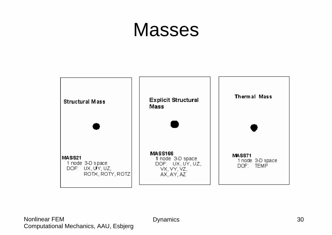
MASS21: Structural Mass
Large deflectionSpecial Features
Key for element coordinate systemKEYOPT(2)
0 - 3-D mass with rotary inertia2 - 3-D mass without rotary inertia3 - 2-D mass with rotary inertia4 - 2-D mass without rotary inertia
KEYOPT(3)
NoneBody Loads
NoneSurface Loads
NoneMaterial Properties
MASSX, MASSY, MASSZ, IXX, IYY, IZZ if KEYOPT(3) = 0MASS if KEYOPT(3) = 2MASS, IZZ if KEYOPT(3) = 3MASS if KEYOPT(3) = 4
Real Constants
UX, UY, UZ, ROTX, ROTY, ROTZ if KEYOPT(3) = 0UX, UY, UZ if KEYOPT(3) = 2UX, UY, ROTZ if KEYOPT(3) = 3UX, UY if KEYOPT(3) = 4
Degrees of Freedom
INodes
MASS21Element Name

Dynamics 7Computational Mechanics, AAU, EsbjergNonlinear FEM
COMBIN14: Spring/Damper
Nonlinear (if CV2 is not zero), Stress stiffening, Large deflection, etc.
Special Features
0 - Linear Solution (default)1 - Nonlinear solution (required if CV2 is non-zero)
KEYOPT(1)
0 - 3-D longitudinal spring-damper1 - 3-D torsional spring-damper2 - 2-D longitudinal spring-damper (2-D elements must lie in an X-Y plane)
KEYOPT(3)
NoneBody Loads
NoneSurface Loads
NoneMaterial Properties
K, CV1, CV2Real Constants
UX, UY, UZ if KEYOPT(3) = 0ROTX, ROTY, ROTZ if KEYOPT(3) = 1UX, UY if KEYOPT(3) = 2etc.
Degrees of Freedom
I, JNodes
COMBIN14Element Name
Dynamics 8Computational Mechanics, AAU, EsbjergNonlinear FEM
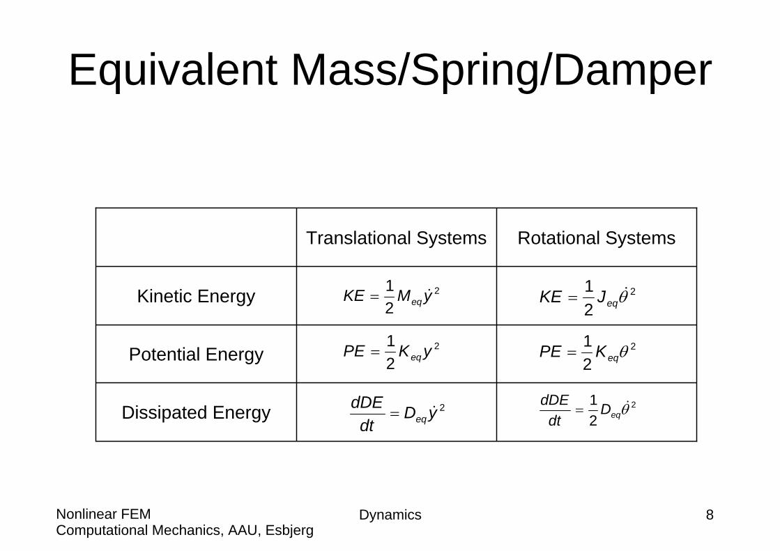
Equivalent Mass/Spring/Damper
Dissipated Energy
Potential Energy
Kinetic Energy
Rotational SystemsTranslational Systems
2
21 yMKE eq=
2
21 yKPE eq=
2yDdt
dDEeq=
2
21 θeqJKE =
2
21 θeqKPE =
2
21 θeqD
dtdDE
=

Computational Mechanics, AAU, EsbjergNonlinear FEM
Design of Spring/Damper in a Recoil Landing System

Dynamics 10Computational Mechanics, AAU, EsbjergNonlinear FEM
Problem Description
Vehicle mass M
Piston
Cylinder
Damper D
Spring K
Rod
Foot

Dynamics 11Computational Mechanics, AAU, EsbjergNonlinear FEM
Modeling Considerations
y
D
K
M
0V(0)y ,0)0(0
===++
yKyyDyM
Dynamics 12Computational Mechanics, AAU, EsbjergNonlinear FEM
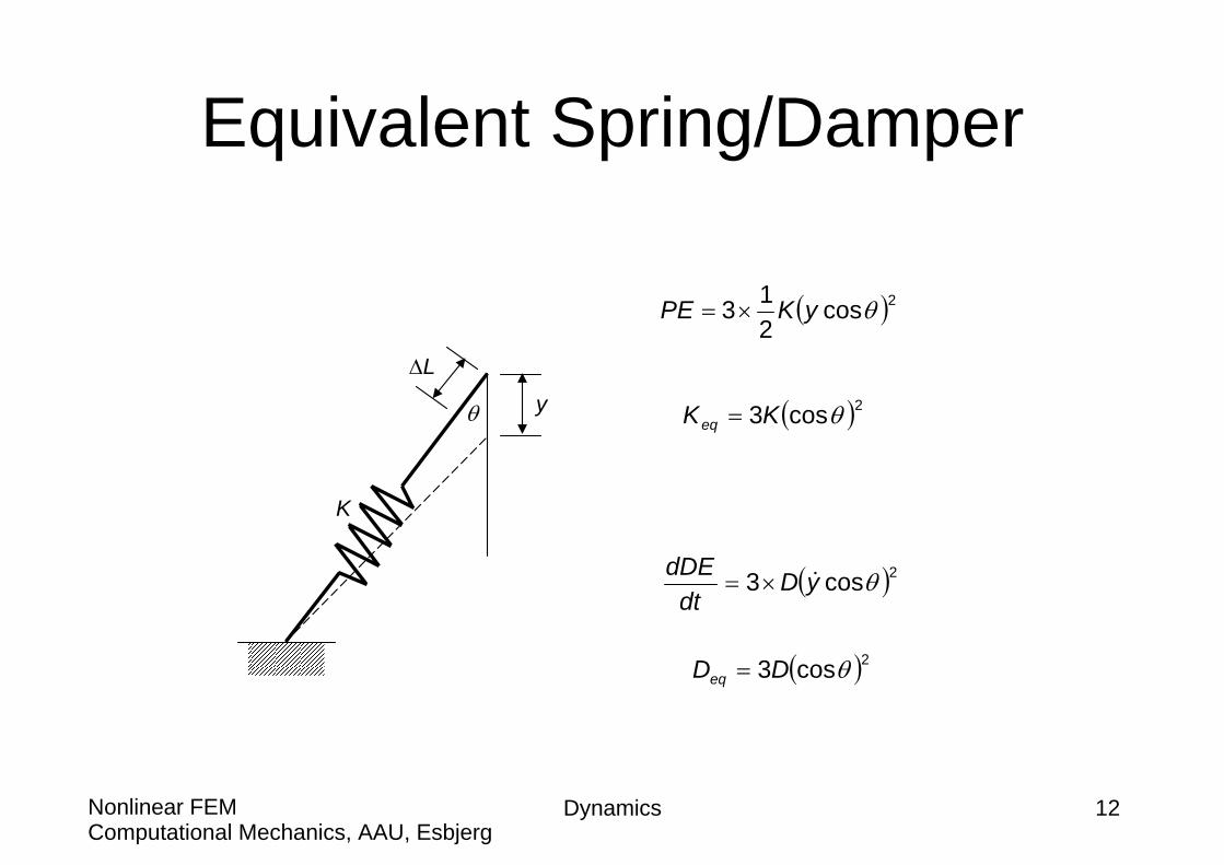
Equivalent Spring/Damper
y
ΔL
K
θ
( )2cos213 θyKPE ×=
( )2cos3 θKKeq =
( )2cos3 θyDdt
dDE×=
( )2cos3 θDDeq =
Dynamics 13Computational Mechanics, AAU, EsbjergNonlinear FEM
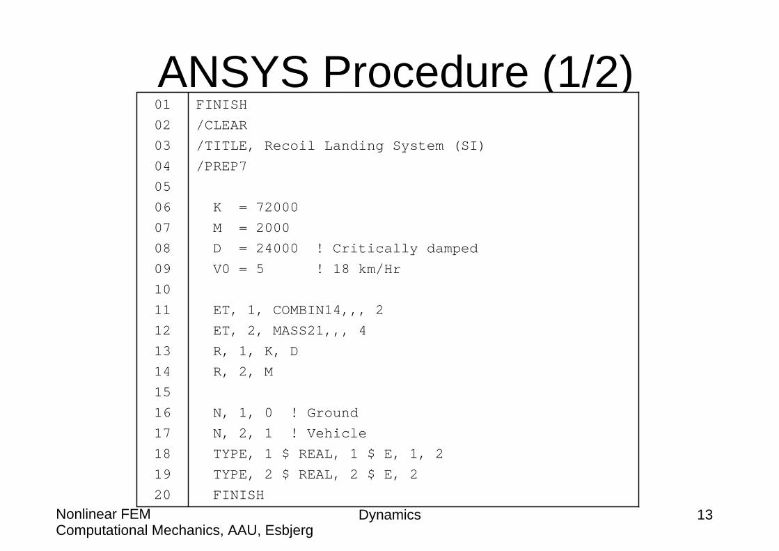
ANSYS Procedure (1/2)FINISH/CLEAR/TITLE, Recoil Landing System (SI)/PREP7
K = 72000M = 2000D = 24000 ! Critically dampedV0 = 5 ! 18 km/Hr
ET, 1, COMBIN14,,, 2ET, 2, MASS21,,, 4R, 1, K, DR, 2, M
N, 1, 0 ! GroundN, 2, 1 ! VehicleTYPE, 1 $ REAL, 1 $ E, 1, 2TYPE, 2 $ REAL, 2 $ E, 2FINISH
0102030405060708091011121314151617181920
Dynamics 14Computational Mechanics, AAU, EsbjergNonlinear FEM
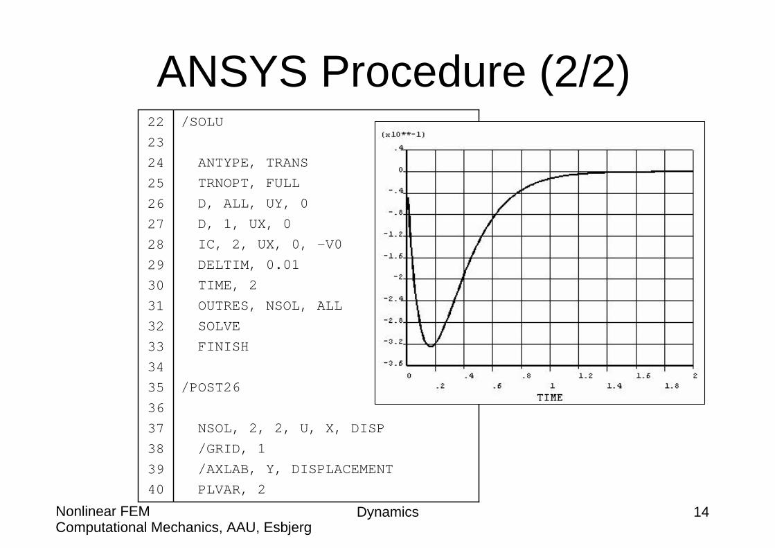
ANSYS Procedure (2/2)/SOLU
ANTYPE, TRANSTRNOPT, FULLD, ALL, UY, 0D, 1, UX, 0IC, 2, UX, 0, -V0DELTIM, 0.01TIME, 2OUTRES, NSOL, ALLSOLVEFINISH
/POST26
NSOL, 2, 2, U, X, DISP/GRID, 1/AXLAB, Y, DISPLACEMENTPLVAR, 2
22232425262728293031323334353637383940
Computational Mechanics, AAU, EsbjergNonlinear FEM
Design of Damper in a Spring Scale

Dynamics 16Computational Mechanics, AAU, EsbjergNonlinear FEM
Problem DescriptionItem placed on platform mass m
Plateform mass Mp
Spring K mass Mk
Rack mass Mr Damper Dmass Md
Calibrated dial Jc
Gear ratio n
Geared magnifier Jg
R
Dynamics 17Computational Mechanics, AAU, EsbjergNonlinear FEM
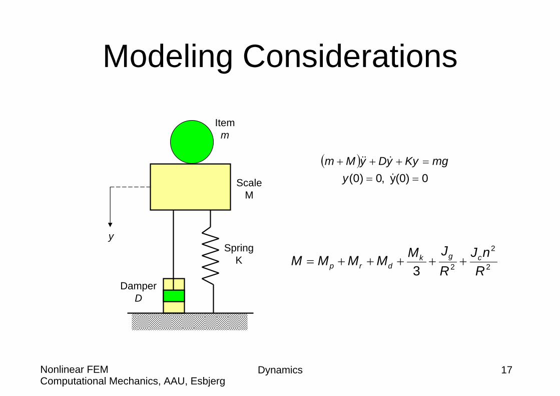
Modeling Considerations
Itemm
ScaleM
SpringK
DamperD
y
( )0(0)y ,0)0( ===+++
ymgKyyDyMm
2
2
23 RnJ
RJMMMMM cgk
drp +++++=

Dynamics 18Computational Mechanics, AAU, EsbjergNonlinear FEM
Lumped Masses (1/4)Lumped Mass for a Spring
L
Vo
V
xdm
Equivalent lumped mass Meq
LxVV o=
621
21 2
0
22 okL ko
L
VMLdxM
LxVdmVKE =⎟⎠⎞
⎜⎝⎛== ∫∫
3k
eqMM =

Dynamics 19Computational Mechanics, AAU, EsbjergNonlinear FEM
Lumped Masses (2/4)Lumped Mass for a Gear-and-Rack Set
R
Mr
JG
Vo
Rolls without slipping
θ
22
2222
21
21
21
21
21
oG
ro
GorGor VRJM
RVJVMJVMKE ⎟
⎠⎞
⎜⎝⎛ +=⎟
⎠⎞
⎜⎝⎛+=+= θ
2RJMM G
req +=

Dynamics 20Computational Mechanics, AAU, EsbjergNonlinear FEM
Lumped Masses (3/4)Lumped Mass for a Geared Shafts Set
J1
J2
N1
N2Jeq
Gears
Shafts
222
2221 2
121
21
21
21
gc
gcg
c
gggggccgg N
NJJ
NN
JJJJKE θθ
θθθ⎥⎥⎦
⎤
⎢⎢⎣
⎡⎟⎟⎠
⎞⎜⎜⎝
⎛+=⎟⎟
⎠
⎞⎜⎜⎝
⎛+=+=
2
⎟⎟⎠
⎞⎜⎜⎝
⎛+=
c
gcgeq N
NJJJ

Dynamics 21Computational Mechanics, AAU, EsbjergNonlinear FEM
Lumped Masses (4/4)Lumped Mass for the Spring Scale System
2
2
RnJJ
MM cgreq
++=
2
2
23 RnJ
RJMMMMM cgk
drp +++++=
Gear set

Dynamics 22Computational Mechanics, AAU, EsbjergNonlinear FEM
ANSYS Procedure (1/2)FINISH/CLEAR/TITLE, Spring Scale (cgs)/PREP7
m = 1500 ! GMeq = 500 ! GK = 3.2E6 ! dyn/cmD = 6.4E4 ! dyn-s/cm
ET, 1, COMBIN14,,, 2ET, 2, MASS21,,, 4R, 1, K, DR, 2, m+Meq
N, 1, 0N, 2, 1TYPE, 1 $ REAL, 1 $ E, 1, 2TYPE, 2 $ REAL, 2 $ E, 2FINISH
0102030405060708091011121314151617181920
Dynamics 23Computational Mechanics, AAU, EsbjergNonlinear FEM
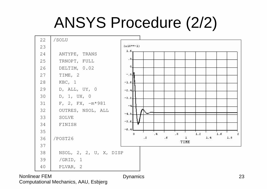
ANSYS Procedure (2/2)/SOLU
ANTYPE, TRANSTRNOPT, FULLDELTIM, 0.02TIME, 2KBC, 1D, ALL, UY, 0D, 1, UX, 0F, 2, FX, -m*981OUTRES, NSOL, ALLSOLVEFINISH
/POST26
NSOL, 2, 2, U, X, DISP/GRID, 1PLVAR, 2
22232425262728293031323334353637383940

Computational Mechanics, AAU, EsbjergNonlinear FEM
Quenching of a Shaft

Dynamics 25Computational Mechanics, AAU, EsbjergNonlinear FEM
Problem Description
T(0)
Tb(0)T(t)
Tb(t)
Shaft
Bath
mb = 1 lb
Before quenching After quenching
ms = 0.069 lb

Dynamics 26Computational Mechanics, AAU, EsbjergNonlinear FEM
Modeling Considerations
ms, Cs, Ts mb, Cb, Tbh, A
Dynamics 27Computational Mechanics, AAU, EsbjergNonlinear FEM
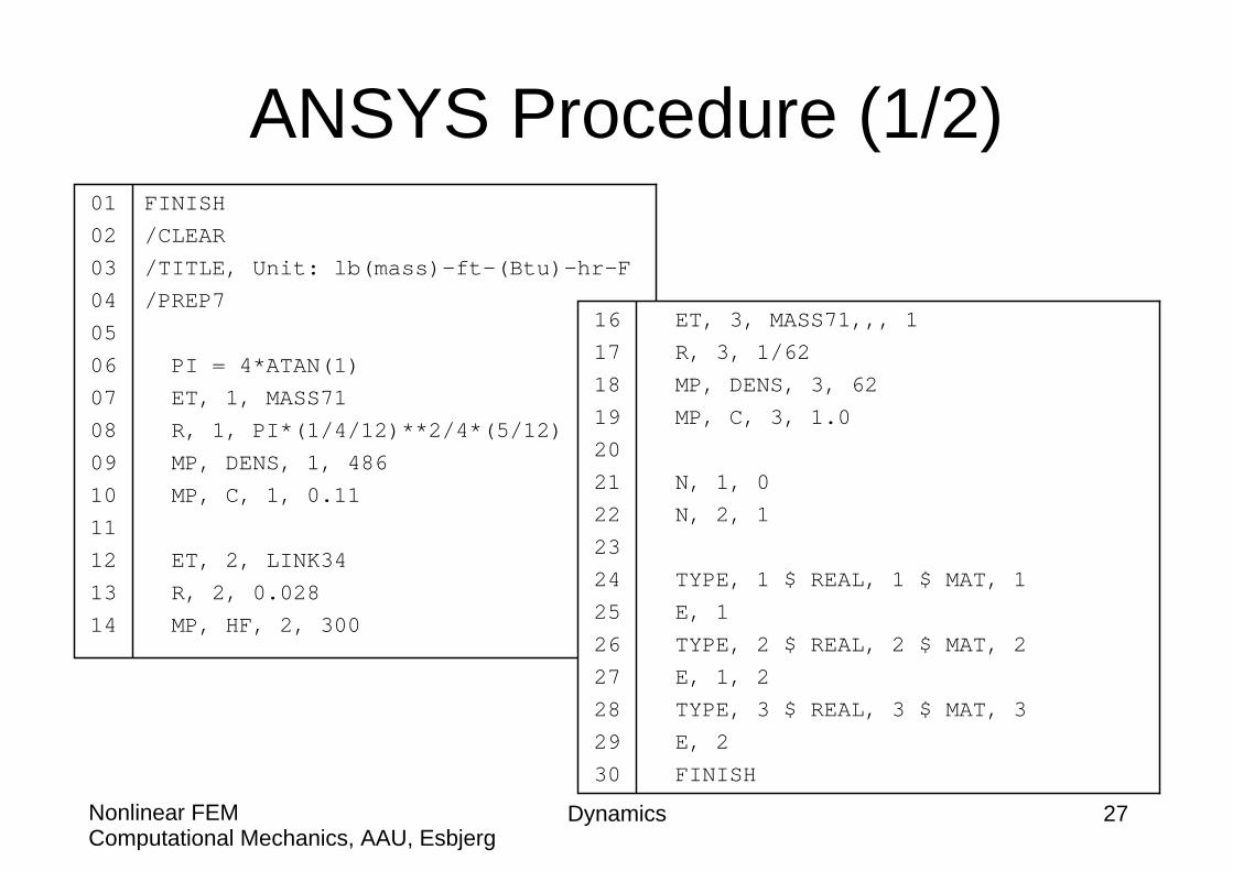
ANSYS Procedure (1/2)FINISH/CLEAR/TITLE, Unit: lb(mass)-ft-(Btu)-hr-F/PREP7
PI = 4*ATAN(1)ET, 1, MASS71R, 1, PI*(1/4/12)**2/4*(5/12)MP, DENS, 1, 486MP, C, 1, 0.11
ET, 2, LINK34R, 2, 0.028MP, HF, 2, 300
0102030405060708091011121314
ET, 3, MASS71,,, 1R, 3, 1/62MP, DENS, 3, 62MP, C, 3, 1.0
N, 1, 0N, 2, 1
TYPE, 1 $ REAL, 1 $ MAT, 1E, 1TYPE, 2 $ REAL, 2 $ MAT, 2E, 1, 2TYPE, 3 $ REAL, 3 $ MAT, 3E, 2FINISH
161718192021222324252627282930

Dynamics 28Computational Mechanics, AAU, EsbjergNonlinear FEM
ANSYS Procedure (2/2)/SOLU
ANTYPE, TRANSTRNOPT, FULLDELTIM, 0.0001KBC, 1TIME, 0.01IC, 1, TEMP, 1300IC, 2, TEMP, 75
OUTRES, NSOL, ALLSOLVEFINISH
/POST26
NSOL, 2, 1, TEMP,, SHAFTNSOL, 3, 2, TEMP,, WATER/GRID, 1PLVAR, 2, 3
3233343536373839404142434445464748495051

Computational Mechanics, AAU, EsbjergNonlinear FEM
Elements Related to Lumped-Mass Systems
Dynamics 30Computational Mechanics, AAU, EsbjergNonlinear FEM
Masses

Dynamics 31Computational Mechanics, AAU, EsbjergNonlinear FEM
Springs/Dampers

Dynamics 32Computational Mechanics, AAU, EsbjergNonlinear FEM
Thermal Links

Dynamics 33Computational Mechanics, AAU, EsbjergNonlinear FEM
Circuit Element
Dynamics 34Computational Mechanics, AAU, EsbjergNonlinear FEM
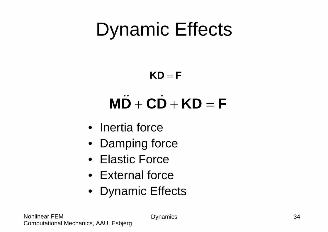
Dynamic Effects
• Inertia force• Damping force• Elastic Force• External force• Dynamic Effects
FKDDCDM =++
FKD =

Dynamics 35Computational Mechanics, AAU, EsbjergNonlinear FEM
Transient Dynamic Analysis
FKDDCDM =++

Dynamics 36Computational Mechanics, AAU, EsbjergNonlinear FEM
Modal Analysis (1/3)
0KDDCDM =++
Dynamics 37Computational Mechanics, AAU, EsbjergNonlinear FEM
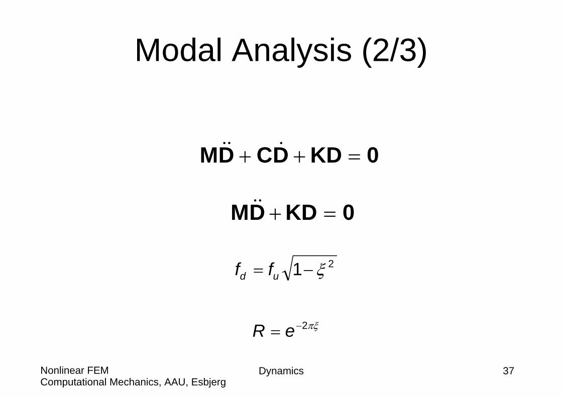
Modal Analysis (2/3)
0KDDCDM =++
0KDDM =+
21 ξ−= ud ff
πξ2−= eR

Dynamics 38Computational Mechanics, AAU, EsbjergNonlinear FEM
Modal Analysis (3/3)
• Avoid resonance• Exploit resonance• Assess structural stiffness• Structural modal degrees of freedom• Further dynamic analyses• etc.
Dynamics 39Computational Mechanics, AAU, EsbjergNonlinear FEM
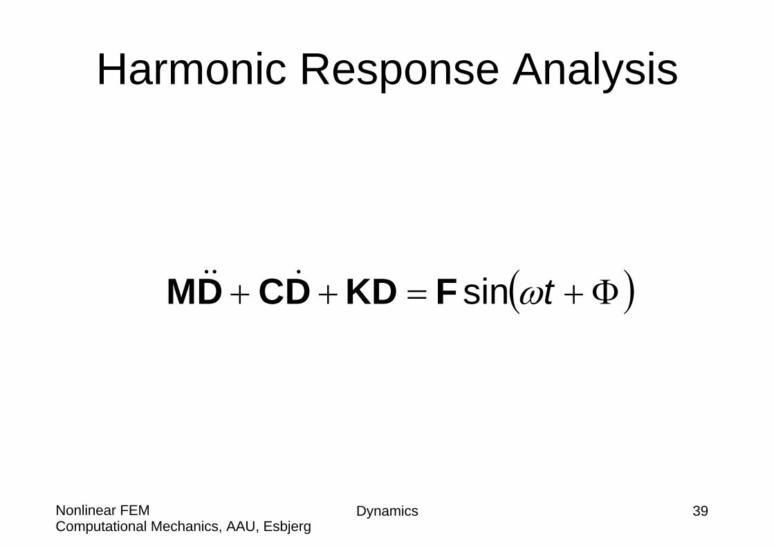
Harmonic Response Analysis
( )Φ+=++ tωsinFKDDCDM

Computational Mechanics, AAU, EsbjergNonlinear FEM
Solution Methods

Dynamics 41Computational Mechanics, AAU, EsbjergNonlinear FEM
Solution Methods
Solution Methods for Equation of Motion
Direct Integration Mode Superposition
Implicit Explicit
ReduceFull Full Reduce

Dynamics 42Computational Mechanics, AAU, EsbjergNonlinear FEM
Solution methods

Dynamics 43Computational Mechanics, AAU, EsbjergNonlinear FEM
Direct Integration
• Implicit method (ANSYS)• Explicit method (LS-DYNA)

Dynamics 44Computational Mechanics, AAU, EsbjergNonlinear FEM
Implicit vs. Explicit Methods
( )ttttttt Δ+Δ−Δ+ = DDDfD ,,...,
( )ttttttt DDDfD ,,..., 2 Δ−Δ−Δ+ =
Implicit method
Explicit method
Dynamics 45Computational Mechanics, AAU, EsbjergNonlinear FEM
Linear vs. nonlinear dynamics• Dynamics or equation of motion:
– The causal relation between the present state and the next state in the future. It is a deterministic rule which tells us what happens in the next time step.
– In the case of a continuous time, the time step is infinitesimally small. Thus, the equation of motion is a differential equation or a system of differential equations:du/dt = F(u), where u is the state and t is the time variable.
– An example is the equation of motion of an undriven and undamped pendulum.
– In the case of a discrete time, the time steps are nonzero and the dynamics is a map:un+1 = F(un), with the discrete time n.
– An example is the baker map. Note, that the corresponding physical time points tn do not necessarily occur equidistantly. Only the order has to be the same. That is, n < m implies tn < tm.
– The dynamics is linear if the causal relation between the present state and the next state is linear. Otherwise it is nonlinear.

Dynamics 46Computational Mechanics, AAU, EsbjergNonlinear FEM
Implicit vs. Explicit• What is the difference between implicit and explicit dynamics? (Difference
between regular ANSYS and ANSYS/LS-DYNA?)
• For computers, matrix multiplication is easy. Matrix inversion is the more computationally expensive operation. The equations we solve in nonlinear, dynamic analyses in ANSYS and in LS-DYNA are:[M]{a} + [C]{v} + [K]{x} = {F}
• Hence, in ANSYS, we need to invert the [K] matrix when using direct solvers (frontal, sparse). Iterative solvers use a different technique from direct solvers, however, the inversion of [K] is the CPU-intensive operation for any 'regular' ANSYS solver, direct or iterative.
• We then can solve for displacements {x}. Of course, with nonlinearities, [K(x)] is also a function of {x}, so we need to use Newton-Raphson method to solve for [K] as well (material nonlinearities and contact get thrown into [K(x)])

Dynamics 47Computational Mechanics, AAU, EsbjergNonlinear FEM
Implicit vs. explicit• In LS-DYNA, on the other hand, we solve for accelerations {a} first.
• It is assumed that the mass matrix is lumped. This basically forces the use of lower-order elements, i.e. for all explicit dynamics codes (ANSYS/LS-DYNA, MSC.Dytran, ABAQUS/Explicit), lower-order elements are used.
• The benefit of doing lumped mass is, if we solve for {a}, then [M], if lumped, is a diagonal mass matrix. This means that inversion of [M] is trivial (diagonal terms only)
• Another way to view it, is that we now have N set of *uncoupled*equations. Hence, we just have to do matrix multiplication, which is less CPU-intensive. Also, [K] does not need to be inverted, and accounting for material nonlinearties and contact is easier.

Dynamics 48Computational Mechanics, AAU, EsbjergNonlinear FEM
Implicit vs. explicit• The terms 'implicit' and 'explicit' refer to time integration
• For example– backward Euler method, that is an example of an implicit time integration scheme– central difference or forward Euler are examples of explicit time integration schemes
• It relates to when you calculate the quantities - either based on current or previous time step.
• In any case, this is a very simplified explanation, and the main point is that implicit time integration is unconditionally stable, whereas explicit time integration is not (there is a critical timestep the timestep delta(t) needs to be smaller than).
• Implicit, e.g. 'regular' ANSYS allows for much larger time steps• Explicit, e.g. LS-DYNA requires much smaller time steps. Also, LS-DYNA requires
very tiny steps, i.e. good for impact/short-duration events, not usually things like maybe creep where the model's time scale may be on the order of hours or more.

Dynamics 49Computational Mechanics, AAU, EsbjergNonlinear FEM
Implicit vs. explicit• 'Regular' ANSYS uses implicit time integration. This means that {x}
is solved for, but we need to invert [K], which means that each iteration is computationally expensive. However, because we solve for {x}, it is implicit, and we don't need very tiny timesteps (i.e., each iteration is expensive, but we usually don't need too many iterations total). – The overall timescale doesn't affect us much (although there are
considerations of small enough timesteps for proper momentum transfer, capturing dynamic response).
• ANSYS/LS-DYNA uses explicit time integration. This means that {a} is solved for, and inverting [M] is trivial -- each iteration is very efficient. However, because we solve for {a}, then determine {x}, it is explicit, and we need very small timesteps (many, many iterations) to ensure stability of solution since we get {x} by calculating {a} first. – (i.e., each iteration is cheap, but we usually need many, many iterations
total)

Dynamics 50Computational Mechanics, AAU, EsbjergNonlinear FEM
Mode Superposition Method
nnCCCC MMMMD ...332211 +++=
Dynamics 51Computational Mechanics, AAU, EsbjergNonlinear FEM
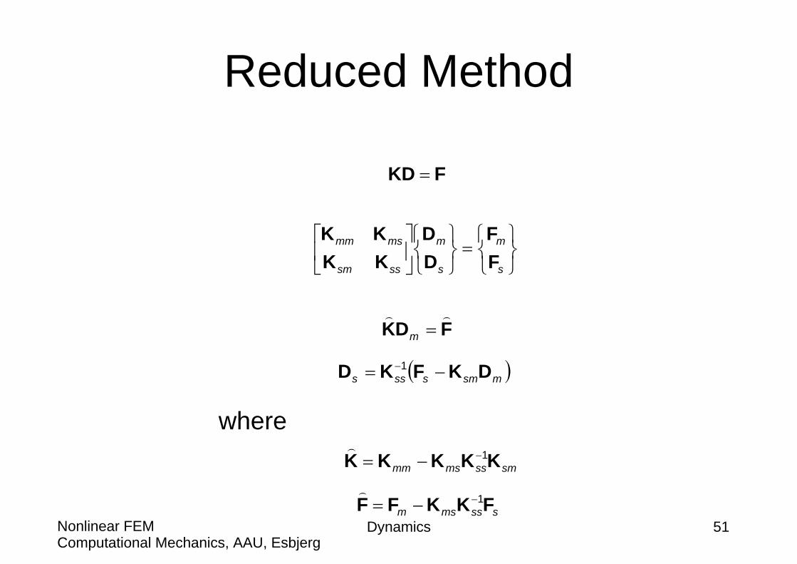
Reduced Method
FKD =
⎭⎬⎫
⎩⎨⎧
=⎭⎬⎫
⎩⎨⎧⎥⎦
⎤⎢⎣
⎡
s
m
s
m
sssm
msmm
FF
DD
KKKK
FDK =m
( )msmssss DKFKD −= −1
smssmsmm KKKKK 1−−=
sssmsm FKKFF 1−−=
where

Dynamics 52Computational Mechanics, AAU, EsbjergNonlinear FEM
Methods for Nonlinear Dynamic Analysis
• For nonlinear analysis, the only methods applicable is DIRECT INTEGRATION method.
• Reduced method can not be used for nonlinear analysis.
• Either implicit or explicit methods can be used.

Computational Mechanics, AAU, EsbjergNonlinear FEM
Mass and Damping

Dynamics 54Computational Mechanics, AAU, EsbjergNonlinear FEM
Consistent vs. Lumped Mass Matrices
⎥⎥⎥⎥⎥⎥⎥⎥
⎦
⎤
⎢⎢⎢⎢⎢⎢⎢⎢
⎣
⎡
⎥⎥⎥⎥⎥⎥⎥⎥
⎦
⎤
⎢⎢⎢⎢⎢⎢⎢⎢
⎣
⎡
xx
xx
xx
xxxxxxxx
xxxxxxxxxx
xx
ROTZUYUX
ROTZUYUX
j
j
j
i
i
i
000000000000000000000000000000
0000
00000000
0000
Consistent mass matrix
Lumped mass matrix
Dynamics 55Computational Mechanics, AAU, EsbjergNonlinear FEM
Damping
• Damping effects is the total of all energy dissipation mechanisms– Hysteresis (solid damping)– Viscous damping– Dry-friction (Coulomb damping)

Dynamics 56Computational Mechanics, AAU, EsbjergNonlinear FEM
Idealization of Structural Damping
• Structural dampings are usually small (2%-7%).
• Equivalent viscous damping is assumed in ANSYS, i.e.,
DCF =D
Dynamics 57Computational Mechanics, AAU, EsbjergNonlinear FEM
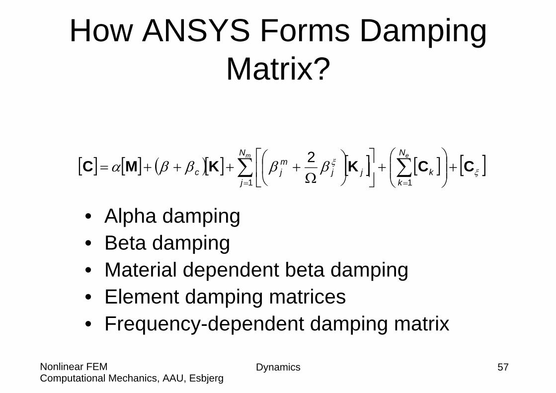
How ANSYS Forms Damping Matrix?
• Alpha damping• Beta damping• Material dependent beta damping• Element damping matrices• Frequency-dependent damping matrix
[ ] [ ] ( )[ ] [ ] [ ] [ ]ξξββββα CCKKMC +⎟⎟⎠
⎞⎜⎜⎝
⎛+⎥
⎦
⎤⎢⎣
⎡⎟⎠⎞
⎜⎝⎛
Ω++++= ∑∑
==
em N
kk
N
jjj
mjc
11
2
Computational Mechanics, AAU, EsbjergNonlinear FEM
Copper Cylinder Impacting on a Rigid Wall

Dynamics 59Computational Mechanics, AAU, EsbjergNonlinear FEM
Problem Description
x
y
L D
Initial Velocity Vo
Dynamics 60Computational Mechanics, AAU, EsbjergNonlinear FEM
Modeling Consideration
• Material: bilinear plastic model.• VISCO106 (2D viscoplastic solid) is
used.• Use axisymmetric model.

Dynamics 61Computational Mechanics, AAU, EsbjergNonlinear FEM
ANSYS Procedure (1/4)FINISH/CLEAR/TITLE, UNITS: SI/PREP7
ET, 1, VISCO106,,, 1MP, EX, 1, 117E9MP, NUXY, 1, 0.35MP, DENS, 1, 8930
TB, BISO, 1TBDATA,, 400E6, 100E6TBPLOT, BISO, 1
RECTNG, 0, 0.0032, 0, 0.0324LESIZE, 1,,, 4LESIZE, 2,,, 20MSHAPE, 0, 2DMSHKEY, 1AMESH, ALLFINISH
010203040506070809101112131415161718192021

Dynamics 62Computational Mechanics, AAU, EsbjergNonlinear FEM
ANSYS Procedure (2/4)/SOLU
ANTYPE, TRANSTRNOPT, FULLNLGEOM, ONIC, ALL, UY, 0, -227NSEL, S, LOC, X, 0D, ALL, UX, 0NSEL, S, LOC, Y, 0D, ALL, UY, 0NSEL, ALL/PBC, U,, ONEPLOT
TIME, 80E-6DELTIM, 0.4E-6KBC, 1OUTRES, ALL, 4SOLVEFINISH
2324252627282930313233343536373839404142

Dynamics 63Computational Mechanics, AAU, EsbjergNonlinear FEM
ANSYS Procedure (3/4)
/POST26
TOPNODE = NODE(0,0.0324,0)
NSOL, 2, TOPNODE, U, Y, DISPDERIV, 3, 2, 1,, VELO
/GRID, 1/AXLAB, X, TIME s/AXLAB, Y, DISPLACEMENT mPLVAR, 2/AXLAB, Y, VELOCITY m/sPLVAR, 3FINISH
4445464748495051525354555657
Dynamics 64Computational Mechanics, AAU, EsbjergNonlinear FEM
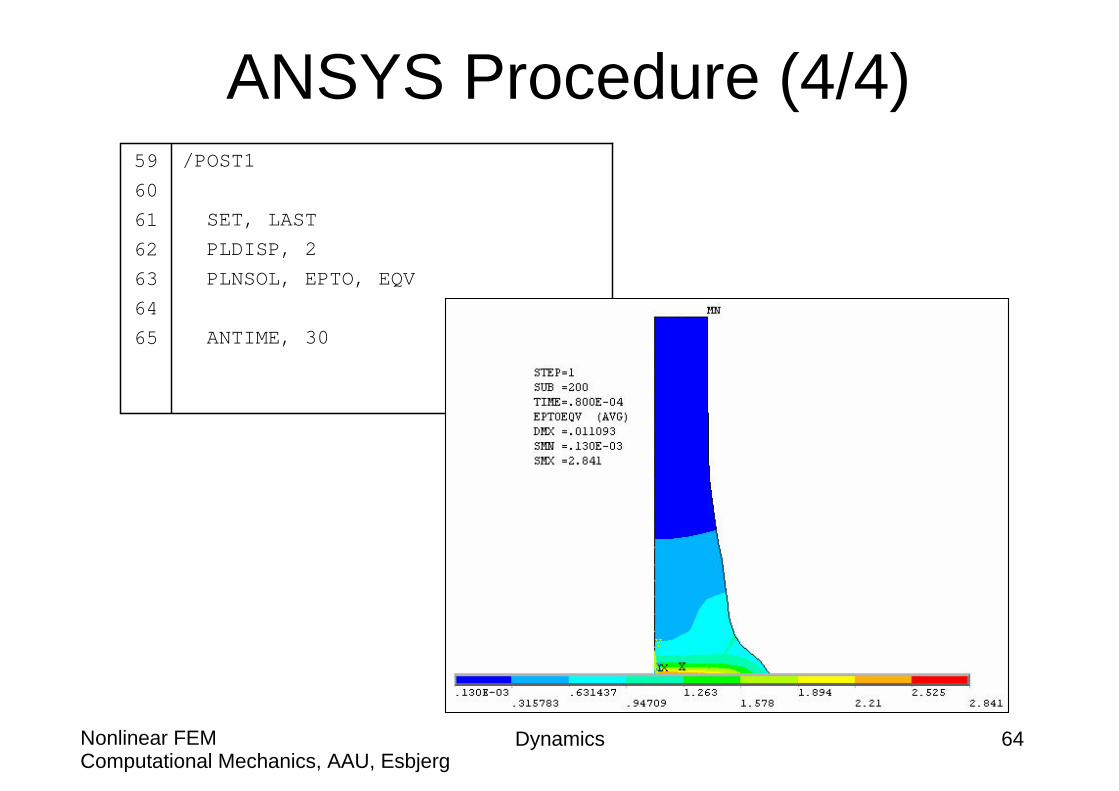
ANSYS Procedure (4/4)/POST1
SET, LASTPLDISP, 2PLNSOL, EPTO, EQV
ANTIME, 30
59606162636465

Computational Mechanics, AAU, EsbjergNonlinear FEM
Dynamic Loads

Dynamics 66Computational Mechanics, AAU, EsbjergNonlinear FEM
Dynamic Loads: An Example/SOLU...F, ... ! 22.5 at the nodesTIME, 0.5 ! Ending timeDELTIM, ... ! Integration stepKBC, 0 ! Ramped loadingAUTOTS, ON ! OptionOUTRES, ... ! OptionSOLVE ! Load step 1
F, ... ! 10 at the nodesTIME, 1 ! Ending timeSOLVE ! Load step 2
FDELE, ... ! Zero the forceTIME, 1.5 ! Ending timeKBC, 1 ! Stepped loadingSOLVE ! Load step 3
010203040506070809101112131415161718
0 0.5 1.0 1.5Time (s)
Force (N)22.5
10

Computational Mechanics, AAU, EsbjergNonlinear FEM
Initial Conditions
Dynamics 68Computational Mechanics, AAU, EsbjergNonlinear FEM
Example: An Stationary Plate Subjected to an Impulse Load
• This is the default initial condition. No input is needed.
Dynamics 69Computational Mechanics, AAU, EsbjergNonlinear FEM
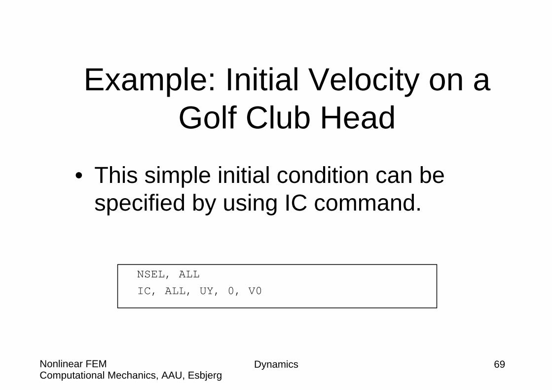
Example: Initial Velocity on a Golf Club Head
• This simple initial condition can be specified by using IC command.
NSEL, ALL
IC, ALL, UY, 0, V0

Dynamics 70Computational Mechanics, AAU, EsbjergNonlinear FEM
Example: Plucking a Cantilever Beam
/SOLUANTYPE, TRANS...TIMINT, OFF ! Transient effects offTIME, 0.001 ! Small time intervalD, ... ! Apply displacement at desired nodesKBC, 1 ! Stepped loadsNSUBST, 2 ! To avoid non-zero velocitySOLVE
TIMINT, ON ! Transient effects onTIME, ... ! Actual time at end of loadDDELE, ... ! Delete the applied displacementSOLVE
0102030405060708091011121314
Dynamics 71Computational Mechanics, AAU, EsbjergNonlinear FEM
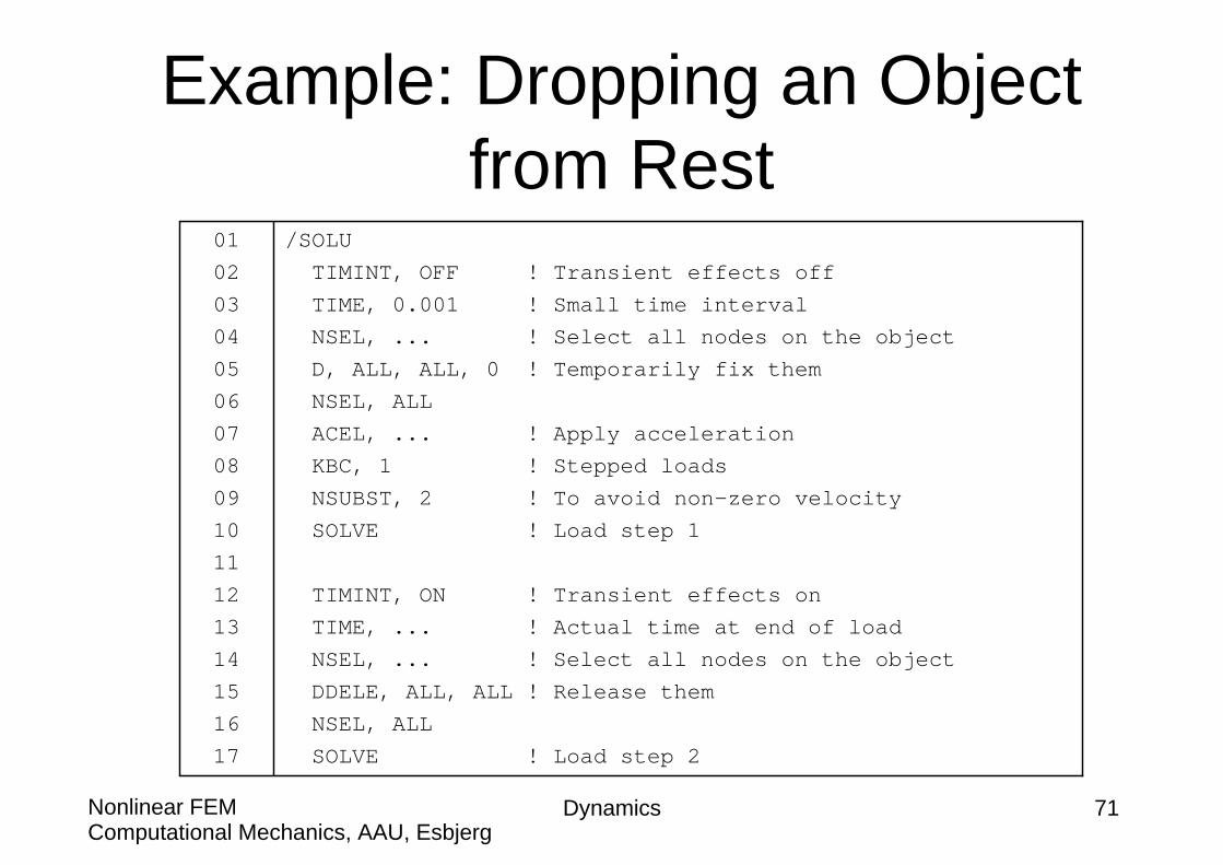
Example: Dropping an Object from Rest
/SOLUTIMINT, OFF ! Transient effects offTIME, 0.001 ! Small time intervalNSEL, ... ! Select all nodes on the objectD, ALL, ALL, 0 ! Temporarily fix themNSEL, ALLACEL, ... ! Apply accelerationKBC, 1 ! Stepped loadsNSUBST, 2 ! To avoid non-zero velocitySOLVE ! Load step 1
TIMINT, ON ! Transient effects onTIME, ... ! Actual time at end of loadNSEL, ... ! Select all nodes on the objectDDELE, ALL, ALL ! Release themNSEL, ALLSOLVE ! Load step 2
0102030405060708091011121314151617

Computational Mechanics, AAU, EsbjergNonlinear FEM
Integration time Steps

Dynamics 73Computational Mechanics, AAU, EsbjergNonlinear FEM
Response Frequency
Response
Time
Minimumresponse
time
20pt ≤Δ

Dynamics 74Computational Mechanics, AAU, EsbjergNonlinear FEM
Abrupt Changes in Loading
0 0.5 1.0 1.5Time (s)
Force (N)
22.5
10

Dynamics 75Computational Mechanics, AAU, EsbjergNonlinear FEM
Contact Frequency
30Tt ≤Δ

Dynamics 76Computational Mechanics, AAU, EsbjergNonlinear FEM
Wave Propagation
cxt
3Δ
≤Δ

Dynamics 77Computational Mechanics, AAU, EsbjergNonlinear FEM
Exercise: Rocket Flight
y
140 in.
Thrust
Time
100 lb
1 sec.1
2
3
![Vega: Nonlinear FEM Deformable Object Simulatorrun.usc.edu/vega/SinSchroederBarbic2012.pdf · Vega: Nonlinear FEM Deformable Object Simulator ... (CalculiX [DW]) deformable ... J.](https://static.fdocuments.net/doc/165x107/5aecb8f27f8b9a3b2e8f8865/vega-nonlinear-fem-deformable-object-nonlinear-fem-deformable-object-simulator.jpg)