EDH-OFW2011

Coupling SUNDIALS with OpenFOAM6

thOpenFOAM Workshop

E. David Huckaby

June 14, 2011

2

Outline

• Motivation

• Mathematics

• Basic Design

• Examples

– Food Web – Steady & Unsteady

– Pitz-Daily

3

Motivation

• Why couple SUNDIALS and OpenFOAM ?

– Improve solution convergence over current segregated solution algorithms

• SUNDIALS vs. alternatives

– Comprehensive – (write own solver)

– Lightweight – Trilinos, PetSC

– User Familiarity (via. Cantera) vs. NITSOL

[1] Luo, Baum, Lohner, 1998, JCP 46, 644-690[2] Pawlowski, Shadid, Simonis, Walker, 2006, SIAM Review 48-2, 700-721[3] Pernice, Tocci, SIAM J. Sci. Comp. 23-2, 398-418[4] Evans, Knoll, Pernice, 2006, JCP 219, 404-417[5] Vuik, Saghir, Boerstoel, 2000, IJ Num. Meth. Fluids 33, 1027-1040[6] Bockelie, Tang, Denison, Wang, Cremer, Chen, 2003, Workshop on Solution Methods for Large Scale Non-Linear Problems[7] Pernice, Zhou, Walker, 1997, University of Utah Center for High Performance Computing

4

SUNDIALS

• Suite of solvers

– CVODE – ode• CVODES – add sensitivity analysis

– KINSOL – nonlinear algebraic equations

– IDA – differential algebraic equations (DAE)• IDAS – add sensitivity analysis

– User supplies the physics function, F

• Features

– Serial & Parallel, “Exact” & Inexact Newton SolversHindmarsh, Brown, Grant, Lee, Serban, Shumaker, Woodward https://computation.llnl.gov/casc/sundials/main.html

),( tyFdtdy

=

0)( =yF

( ) 0,, =tyyF

5

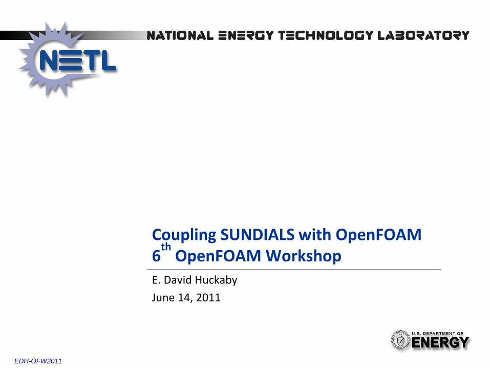
Nonlinear Iteration

• At each time step a DAE or ODE system form nonlinear algebraic system

• Newton

– Solve

– Until

• Approximate Newton (Picard, SIMPLE, …)

• Inexact Newton

FJsxxxFsxJ

x

kkkkkk

∇=+=−= +1)()(

)()( kkkappr xFsxJ −=

)()()( kk

kkk xFxFsxJ η<+

relabsk xFxF εε +<+ )()( 01

Knoll and Keys, 2006, JCP 193, 357–397Collier, Hindmarsh, Serban, Woodward,KINSOL v.2.6

6

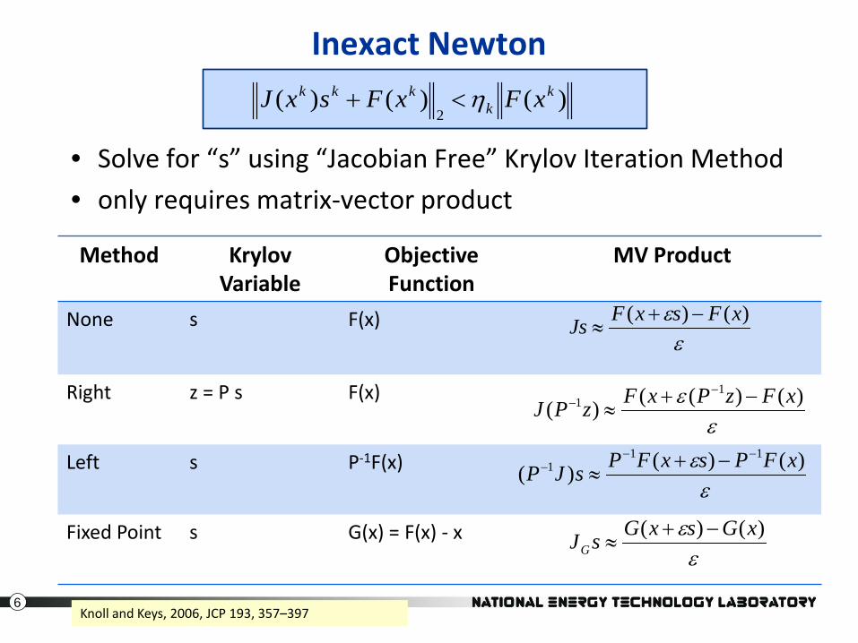
Method KrylovVariable

ObjectiveFunction

MV Product

None s F(x)

Right z = P s F(x)

Left s P-1F(x)

Fixed Point s G(x) = F(x) - x

Inexact Newton

• Solve for “s” using “Jacobian Free” Krylov Iteration Method

• only requires matrix-vector product

)()()(2

kk

kkk xFxFsxJ η<+

εε )()(()(

11 xFzPxFzPJ −+

≈−

−

εε )()()(

111 xFPsxFPsJP

−−− −+

≈

εε )()( xGsxGsJG

−+≈

εε )()( xFsxFJs −+

≈

Knoll and Keys, 2006, JCP 193, 357–397

7

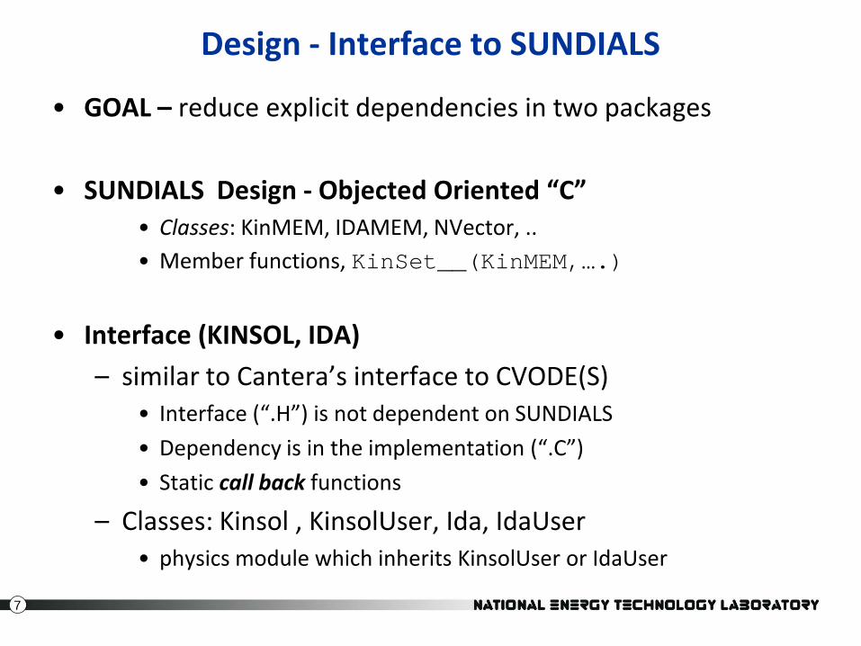
Design - Interface to SUNDIALS

• GOAL – reduce explicit dependencies in two packages

• SUNDIALS Design - Objected Oriented “C”• Classes: KinMEM, IDAMEM, NVector, ..• Member functions, KinSet__(KinMEM,….)

• Interface (KINSOL, IDA)

– similar to Cantera’s interface to CVODE(S)• Interface (“.H”) is not dependent on SUNDIALS

• Dependency is in the implementation (“.C”)

• Static call back functions

– Classes: Kinsol , KinsolUser, Ida, IdaUser• physics module which inherits KinsolUser or IdaUser

8

Design – Physics Module

• Physics Modules (OpenFOAM)

– Turn solvers into objects

– Class contains fields AND equations• Similar to turbulence and radiation models

– No dependence on SUNDIALS

• SUNDIALS/OpenFOAM Physics Module

– Inherits from KinsolUser or IDAUser

– Container for OpenFOAM solver object• FoodWeb, Incompressible Flow, …

9

Outline

• Motivation

• Mathematics

• Basic Design

• Examples

– Food Web – Steady & Unsteady

– Pitz-Daily

10

• Reaction-Diffusion Equation

“ci“: M prey & M predators

– Steady (KINSOL) – M = 3

– Unsteady (IDA) – M = 1

Food Web Model

015.01 ==== βαpreypred dd

5103)0,(1)0( ×==== txckc predprey

( ) ),( cxfcdtcm iii

ii

+∇⋅∇=∂∂

( )5

2

10)0,(

)1()1(1610)0,(

==

−−+==

txc

yyxxitxc

pred

preyprey

1000505.01 ==== βαpreypred dd

44 105101

00

00

−×===

−−

−−−−−−

=

GEA

AEEAEE

GGAGGA

aij

11

01

−==

==

preyprey

predprey

bbmm

+= ∑

≠ jijijiii caxgbccxf )(),(

( ))4sin()4sin(1)( yxyxxg ππβα +++=

Brown, 1986, SIAM J. Applied Math, v.46, no. 3Collier and Serban (KINSOL), Hindmarsh, Serban, Collier (IDA)

Model Parameters

11

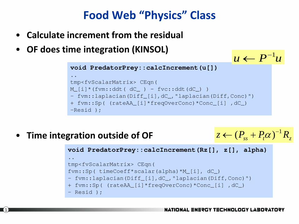
Food Web “Physics” Class

• Calculate increment from the residual

• OF does time integration (KINSOL)

• Time integration outside of OF

void PredatorPrey::calcIncrement(u[])..tmp<fvScalarMatrix> CEqn(M_[i]*(fvm::ddt( dC_ ) - fvc::ddt(dC_) )- fvm::laplacian(Diff_[i],dC_,"laplacian(Diff,Conc)")+ fvm::Sp( (rateAA_[i]*freqOverConc)*Conc_[i] ,dC_)-Resid );

void PredatorPrey::calcIncrement(Rz[], z[], alpha)..tmp<fvScalarMatrix> CEqn(fvm::Sp( timeCoeff*scalar(alpha)*M_[i], dC_)- fvm::laplacian(Diff_[i],dC_,"laplacian(Diff,Conc)")+ fvm::Sp( (rateAA_[i]*freqOverConc)*Conc_[i] ,dC_)- Resid );

uPu 1−←

ztss RPPz 1)( −+← α

12

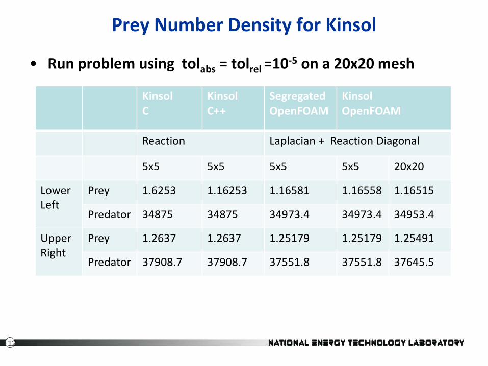
Prey Number Density for Kinsol

• Run problem using tolabs = tolrel =10-5 on a 20x20 mesh

KinsolC

KinsolC++

SegregatedOpenFOAM

KinsolOpenFOAM

Reaction Laplacian + Reaction Diagonal

5x5 5x5 5x5 5x5 20x20

Lower Left

Prey 1.6253 1.16253 1.16581 1.16558 1.16515

Predator 34875 34875 34973.4 34973.4 34953.4

Upper Right

Prey 1.2637 1.2637 1.25179 1.25179 1.25491

Predator 37908.7 37908.7 37551.8 37551.8 37645.5

13

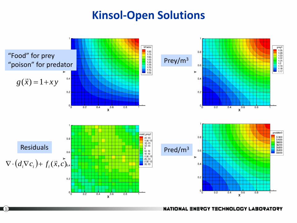
Kinsol-Open Solutions

yxxg +=1)(

( ) ),( cxfcd iii

+∇⋅∇

Prey/m3

Pred/m3

“Food” for prey “poison” for predator

Residuals

14

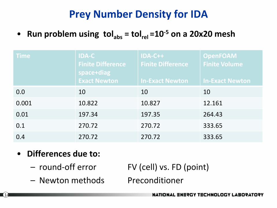
Prey Number Density for IDA

• Run problem using tolabs = tolrel =10-5 on a 20x20 mesh

•

• Differences due to:

– round-off error FV (cell) vs. FD (point)

– Newton methods Preconditioner

Time IDA-CFinite Differencespace+diagExact Newton

IDA-C++Finite Difference

In-Exact Newton

OpenFOAMFinite Volume

In-Exact Newton

0.0 10 10 10

0.001 10.822 10.827 12.161

0.01 197.34 197.35 264.43

0.1 270.72 270.72 333.65

0.4 270.72 270.72 333.65

15

Prey Number Density

Green - OpenFOAM (cell)Red -IDA-C++ (point)Blue – IDA-C++ (point->cell)

16

Final Prey Number Density

IDA -C++

IDA-OpenFOAM

17

Incompressible Flow

• Simple class for (steady & unsteady) incompressible flow based on SIMPLE algorithm

– Residual & Left - Preconditioner for Ida

– Residual & Right - Preconditioner for Kinsol

– Fixed-Point Residual Preconditioning for Kinsol• Necessarily have a standard SIMPLE solver

• Advantageous as solver complexity increases

• <?>SimpleFoam solver

– Provides interfaces between simple class and SUNDIALS packages

18

Laminar Pitz Daily

KinsolRight Precond

KinsolFixed Point

Picard SIMPLE

Time(s) 129 s 138 s 198 s 146 s

Machine zero Machine zero 1000 iters 1000 iters

Mass L2 1.1 e-12 7.6 e-11 2e-7 1.32

Mass abs-max 8.9 e-12 9.1 e-10 4.77e-6 83.3

Mom. L2 2.1 e-12 9.4e-8 0.016 98.9

Mom. abs-max 9.0 e-12 1.2e-6 0.080 5314

• Tested on Pitz-Daily with ν = 0.01 m/s2

19

Laminar Pitz-Daily

• Velocity Profiles are nearly identical

12 m/s 0 m/s 5 m/s -1 in

+1 in

Kinsol-Right

Kinsol-Fixed Point

Picard-SIMPLE

20

Turbulent Pitz-Daily

• Solver Approach

1. nonlinear iteration on velocity & pressure followed by2. N SIMPLE sweeps on U, p & M1 turbulence corrections

3. M2 turbulence corrections

• System is much less robust

– Selection of input parameters • loose tolerance at the beginning – tighten toward convergence

• “step-size”

– Turbulence model • Reynolds stress seemed to work better

– Need “Globalization Methods”

21

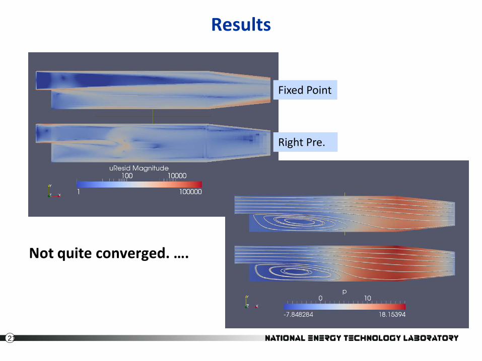
Results

Fixed Point

Right Pre.

Not quite converged. ….

22

Future Work

• Testing and exploration of existing software interfaces

– Solution Strategies• Improve variable and residual scaling

– Ida with incompressible flow

– Include turbulence models in nonlinear iteration

• Code “clean up”

– generalization, templates, better names, comments,..

– Extend to other physical systems

– Additional Capabilities• Sensitivity Analysis – IDAS, CVodeS, ..

• Alternative Packages - NITSOL, Trillinos (NOX), ..