Coupling of Integrated Biosphere Simulator to Regional ...

Coupling of Integrated Biosphere Simulator to Regional Climate Model Version 3

JONATHAN M. WINTER

Massachusetts Institute of Technology, Cambridge, Massachusetts

JEREMY S. PAL

Loyola Marymount University, Los Angeles, California

ELFATIH A. B. ELTAHIR

Massachusetts Institute of Technology, Cambridge, Massachusetts

(Manuscript received 19 March 2008, in final form 4 September 2008)

ABSTRACT

A description of the coupling of Integrated Biosphere Simulator (IBIS) to Regional Climate Model version

3 (RegCM3) is presented. IBIS introduces several key advantages to RegCM3, most notably vegetation

dynamics, the coexistence of multiple plant functional types in the same grid cell, more sophisticated plant

phenology, plant competition, explicit modeling of soil/plant biogeochemistry, and additional soil and snow

layers.

A single subroutine was created that allows RegCM3 to use IBIS for surface physics calculations. A revised

initialization scheme was implemented for RegCM3–IBIS, including an IBIS-specific prescription of vege-

tation and soil properties.

To illustrate the relative strengths and weaknesses of RegCM3–IBIS, one 4-yr numerical experiment was

completed to assess ability of both RegCM3–IBIS (with static vegetation) and RegCM3 with its native land

surface model, Biosphere–Atmosphere Transfer Scheme 1e (RegCM3–BATS1e), to simulate the energy and

water budgets. Each model was evaluated using the NASA Surface Radiation Budget, FLUXNET micro-

meteorological tower observations, and Climate Research Unit Time Series 2.0. RegCM3–IBIS and

RegCM3–BATS1e simulate excess shortwave radiation incident and absorbed at the surface, especially

during the summer months. RegCM3–IBIS limits evapotranspiration, which allows for the correct estimation

of latent heat flux, but increases surface temperature, sensible heat flux, and net longwave radiation.

RegCM3–BATS1e better simulates temperature, net longwave radiation, and sensible heat flux, but sys-

tematically overestimates latent heat flux. This objective comparison of two different land surface models will

help guide future adjustments to surface physics schemes within RegCM3.

1. Introduction

In January 1981, the New York Times article ‘‘Down

on the farm, higher prices’’ (King 1981) explained the

economic impacts of drought, predicting a 10%–15%

increase in average U.S. consumer food bills resulting

from a lack of rainfall in 1980. Agricultural productivity

is strongly correlated to soil moisture, as examined by

studies such as that of Claassen and Shaw (1970). As the

world’s food supply continues to be taxed by burgeoning

populations, a greater percentage of arable land will need

to be utilized and land currently producing food must

become more efficient.

The need for efficient use of arable land is clear, but

even in regions of the world where weather and climate

forecasts are most accurate, the fluctuations in rainfall

and temperature that dictate the productivity of agri-

cultural areas are largely unpredictable beyond synoptic

time scales at a useful resolution.

One approach used to gain a better understanding of

local land–atmosphere processes is regional modeling.

Though limited in predictive ability by the use of bound-

ary conditions and prescribed sea surface temperatures

(SSTs), regional models are able to resolve important

processes at sub–general circulation model (GCM) spa-

tial scales. Regional Climate Model version 3 (RegCM3)

Corresponding author address: Jonathan M. Winter, MIT Bldg.

48-216, 15 Vassar Street, MA 02139.

E-mail: [email protected]

15 MAY 2009 W I N T E R E T A L . 2743

DOI: 10.1175/2008JCLI2541.1

� 2009 American Meteorological Society

was chosen because of its proficiency in simulating en-

ergy and water dynamics throughout North America

(Pal et al. 2000). Additionally, RegCM3 has been used

extensively in a variety of climate studies, including an

exploration of the sensitivity of regional climate to de-

forestation in the Amazon basin (Eltahir and Bras

1994), an investigation of the impact of tundra ecosys-

tems on the surface energy budget and climate of Alaska

(Lynch et al. 1999), and the implementation of a large-

scale cloud/precipitation scheme and model verification

using satellite- and station-based datasets (Pal et al.

2000). Several previous studies have employed coupled

regional climate–dynamic vegetation models, including

Eastman et al. (2001) and Kumar et al. (2008).

Without validation, models are of limited use. RegCM3

coupled to Integrated Biosphere Simulator (RegCM3–

IBIS) and RegCM3 with its current land surface model,

Biosphere–Atmosphere Transfer Scheme 1e (RegCM3–

BATS1e), are evaluated against observations to gain a

better understanding of the current state of surface

physics modeling.

2. Model and dataset description

This section briefly describes RegCM3, IBIS, and the

datasets used in the analyses.

a. RegCM3

RegCM3 is a three-dimensional, sigma-coordinate,

hydrostatic, compressible, primitive-equation regional

climate model that was originally developed at the

National Center for Atmospheric Research (NCAR)

and is currently maintained at the International Centre

for Theoretical Physics (ICTP; Pal et al. 2007). RegCM3

is a descendant of the NCAR Regional Climate Model

(RegCM), which was developed from the work of

Dickinson et al. (1989), Giorgi and Bates (1989), and

Giorgi (1990). RegCM was primarily built using the dy-

namical core of the fourth-generation Pennsylvania State

University (PSU)–NCAR Mesoscale Model (Anthes

et al. 1987).

Key components of RegCM3 include the following:

the atmospheric radiation transfer computations of the

NCAR Community Climate Model version 3 (CCM3;

Kiehl et al. 1996); the planetary boundary layer (PBL)

scheme of Holtslag et al. (1990); BATS1e for land sur-

face processes (Dickinson et al. 1993); the ocean flux

parameterization of Zeng et al. (1998); Subgrid Explicit

Moisture Scheme (SUBEX), a resolvable-scale (non-

convective) cloud and precipitation formulation created

by Pal et al. (2000); and three convection parameteriza-

tion packages—the Emanuel (1991) scheme, the Grell

(1993) scheme, and the Kuo scheme of Anthes (1977).

b. Description of surface physics models

IBIS, which was developed at the University of

Wisconsin—Madison by Foley et al. (1996), is a dynamic

global vegetation model (DGVM) that uses a modular,

physically consistent framework to perform integrated

simulations of water, energy, and carbon fluxes. A com-

plete description of the biophysical processes contained

in IBIS can be found in Pollard and Thompson (1995).

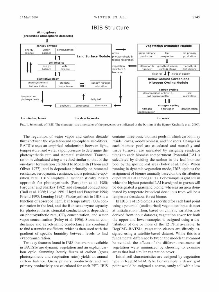
IBIS includes four modules organized with respect to

their temporal scale: land surface processes, soil bioge-

ochemistry, vegetation dynamics, and vegetation phe-

nology (Fig. 1). Based on the Land Surface Transfer

Scheme (LSX) by Thompson and Pollard (1995a,b), the

IBIS land surface module simulates energy, water, car-

bon, and momentum balances of the soil–vegetation–

atmosphere system (Kucharik et al. 2000). The land

surface module contains two vegetation layers, three

snow layers, and up to six soil layers, allowing it to resolve

changes in state variables both within the lower (shrubs,

grasses) and upper (trees) canopies, as well as in each

individual layer of soil and snow (Kucharik et al. 2000).

BATS1e is a comprehensive model of land surface

processes that can be run offline, coupled to a GCM, or

coupled to RegCM3 (Dickinson et al. 1993). BATS1e

simulates a single-layer canopy with two soil layers and

one snow layer. Full documentation of BATS1e can be

found in Dickinson et al. (1993). BATS1e performs the

following six major tasks: initializing vegetation and soil

characteristics; calculating surface albedo, drag coeffi-

cient, and momentum drag; computing leaf area index

(LAI), wind in the canopy, stomatal resistance, and other

vegetation parameters; computing transpiration, leaf

evaporation rates, dew formation, and leaf temperature;

determining soil moisture, soil temperature, runoff, and

snow cover; and calculating sensible and latent heat fluxes.

While the models are similar, some significant dif-

ferences exist in the underlying structure, as well as at

initialization.

Many differences are related to the more detailed

treatment of vegetation in IBIS. Each grid cell in

BATS1e has an assigned vegetation class with parameters

that define the vegetation albedo, soil properties, frac-

tional vegetation cover, roughness characteristics, etc.

IBIS has a two-layer canopy in which any number of plant

functional types (PFTs) may exist in each grid cell. PFTs

are explicitly allowed to compete for light and water.

For most calculations, including water and carbon fluxes,

each PFT is treated separately and then aggregated to

determine grid cell values. Canopy height and roughness

parameters are variable in IBIS, but fixed in BATS1e.

LAI is a function of temperature in both models, but LAI

is also influenced by soil moisture in IBIS.

2744 J O U R N A L O F C L I M A T E VOLUME 22

The regulation of water vapor and carbon dioxide

fluxes between the vegetation and atmosphere also differs.

BATS1e uses an empirical relationship between light,

temperature, and water vapor pressure to determine the

photosynthetic rate and stomatal resistance. Transpi-

ration is calculated using a method similar to that of the

one-layer formulation credited to Monteith (Thom and

Oliver 1977), and is dependent primarily on stomatal

resistance, aerodynamic resistance, and a potential evapo-

ration rate. IBIS employs a mechanistically based

approach for photosynthesis (Farquhar et al. 1980;

Farquhar and Sharkey 1982) and stomatal conductance

(Ball et al. 1986; Lloyd 1991; Lloyd and Farquhar 1994;

Friend 1995; Leuning 1995). Photosynthesis in IBIS is a

function of absorbed light, leaf temperature, CO2 con-

centration in the leaf, and the Rubisco enzyme capacity

for photosynthesis; stomatal conductance is dependent

on photosynthetic rate, CO2 concentration, and water

vapor concentration (Foley et al. 1996). Stomatal con-

ductance and aerodynamic conductance are combined

to find a transfer coefficient, which is then used with the

gradient of specific humidity between levels to find

evapotranspiration.

Two key features found in IBIS that are not available

in BATS1e are dynamic vegetation and an explicit car-

bon cycle. Summing hourly fluxes of carbon (gross

photosynthetic and respiration rates) yields an annual

carbon balance. Gross primary productivity and net

primary productivity are calculated for each PFT. IBIS

contains three basic biomass pools in which carbon may

reside: leaves, woody biomass, and fine roots. Changes in

each biomass pool are calculated and mortality and

tissue turnover are simulated by assigning residence

times to each biomass compartment. Potential LAI is

calculated by dividing the carbon in the leaf biomass

pool by the specific leaf area (Foley et al. 1996). When

running in dynamic vegetation mode, IBIS updates the

assignment of biomes annually based on the distribution

of potential LAI among PFTs. For example, a grid cell in

which the highest potential LAI is assigned to grasses will

be designated a grassland biome, whereas an area dom-

inated by temperate broadleaf deciduous trees will be a

temperate deciduous forest biome.

In IBIS, 1 of 15 biomes is specified for each land point

using a potential (undisturbed) vegetation input dataset

at initialization. Then, based on climatic variables also

derived from input datasets, vegetation cover for both

the upper and lower canopies is assigned using a dis-

tribution of one or more of the 12 PFTs available. In

RegCM3–BATS1e, vegetation classes are directly as-

signed using a satellite-based dataset. While this is a

fundamental difference between the models that cannot

be avoided, the effects of the different treatments of

vegetation were minimized by choosing to examine

areas that had similar vegetation cover.

Initial soil characteristics are assigned by vegetation

type in RegCM3–BATS1e. For example, a desert grid

point would be assigned a coarse, sandy soil with a low

FIG. 1. Schematic of IBIS. The characteristic time scales of the processes are indicated at the bottom of the figure (Kucharik et al. 2000).

15 MAY 2009 W I N T E R E T A L . 2745

soil water fraction, while for a deciduous forest, a wet-

ter, finer soil with silt and clay would be specified. The

original version of IBIS sets soil moisture to a constant

for all grid cells; however, a new scheme for initializing

soil moisture and temperature in RegCM3–IBIS was

developed. Because IBIS is available as an offline model,

which is forced using prescribed atmospheric data, it can

be run for decades relatively inexpensively with respect

to computational time. By modifying the offline version

of IBIS, it is possible to output the soil moisture, soil ice,

and soil temperature for each soil layer. This dataset can

then be used in the initialization subroutine of RegCM3–

IBIS, allowing for a more accurate (relative to the off-

line version of IBIS) initialization of soil moisture and

temperature.

c. Datasets

RegCM3–IBIS and RegCM3–BATS1e were evalu-

ated using three observational datasets; a brief de-

scription of each is provided. The Climate Research

Unit (CRU) Time Series 2.0 (TS2.0) dataset contains

observed surface temperature, water vapor pressure,

and precipitation resampled on a 0.58 3 0.58 regular

latitude–longitude grid (Mitchell et al. 2004). Some as-

pects of the energy budget were evaluated using the

National Aeronautics and Space Administration (NASA)

Surface Radiation Budget (SRB) dataset, obtained from

the NASA Langley Research Center Atmospheric Science

Data Center (available online at http://eosweb.larc.nasa.

gov). After processing, the dataset has a 1.08 3 1.08 res-

olution on a regular latitude–longitude grid. FLUXNET

is a network of micrometeorological tower sites that

provides eddy covariance flux measurements of carbon,

water vapor, and energy between the land surface and

atmosphere. Currently the network includes over 400

tower sites operating both on a long-term and continuous

basis (Baldocchi et al. 2001).

Three FLUXNET sites were chosen based on their

proximity to agriculturally productive areas and the avail-

ability of data for the time period examined. Bondville,

Illinois (40.08N, 88.38W), is an agricultural site with an

annual rotation between soybeans (1998) and corn

(1997 and 1999). The climate is temperate continental

and the vegetation type is cropland. Park Falls, Wisconsin

(45.98N, 90.38W), is situated in the Chequamegon

National Forest. The vegetation cover at this site is

evergreen needleleaf/temperate forest and the cli-

mate is cool continental. Little Washita Watershed

(35.08N, 98.08W) is located near Chickasha, Oklahoma.

The climate is temperate continental and the vegetation

type is grassland. The FLUXNET data used in this

analysis are point measurements, generally taken

hourly, and are derived from the FLUXNET Marconi

Conference gap-filled flux and meteorology data (Falge

et al. 2005).

It is important to note that there are some errors as-

sociated with the FLUXNET observations, and that the

energy budget does not close. To address this, the en-

ergy budget of the FLUXNET observations was closed

using the methodology of Twine et al. (2000). Specifi-

cally, the ground heat flux was subtracted from the net

radiation to find the available energy, and then the la-

tent and sensible heat fluxes were scaled while pre-

serving the Bowen ratio to match the available energy.

At Park Falls no soil heat flux data are available. The

closest proxy data for the soil heat flux at Park Falls is

Willow Creek, Wisconsin. Approximately 22 km from

Park Falls, the Willow Creek soil heat flux for 1999 was

used for the soil heat flux at Park Falls.

3. Coupling

Building on the work of J. S. Pal (2002, personal

communication) and Delire et al. (2002), IBIS was cou-

pled to RegCM3 with one subroutine responsible for

interfacing the two models, as well as additional minor

changes to the RegCM3 and IBIS source codes.

The coupling of RegCM3 and IBIS involved the fol-

lowing five primary tasks: initialization, passing varia-

bles from RegCM3 to IBIS, passing variables from IBIS

to RegCM3, restart, and output. Consideration was given

to future developments of each model, and, when pos-

sible, changes to the original IBIS and RegCM3 code

were avoided.

The offline version of IBIS creates its input variables

from seven files containing monthly mean climatologies

that are perturbed by a weather generator and used by

the rest of the model. None of the datasets used by the

offline version of IBIS are needed in RegCM3–IBIS

except at initialization, where climatic conditions and

the distribution of biomes are required for the allocation

of PFTs within the domain. Instead, 12 forcing fields are

passed from RegCM3 to IBIS at every time step. These

variables are listed in Fig. 2. The transfer of data from

IBIS to RegCM3 is handled in much the same way as the

input. A list of variables passed from IBIS to RegCM3

is included in Fig. 2. The coupling time scale of RegCM3

and IBIS is a user-defined value based on the time step

of the simulation.

The vegetation dataset used by the offline version of

IBIS was added to the RegCM3 preprocessor, allowing

IBIS biomes to be assigned during initialization. Two

additional biomes, inland water and ocean, were added

to the set of biomes contained in the offline version.

Another change to the preprocessing of RegCM3–

IBIS is the way in which soil types are defined. Two files


are read in, with one containing the percentage of clay

and the other the percentage of sand. These data are

then interpolated to the RegCM3 grid and assigned phys-

ical properties such as porosity, albedo, density, etc., based

on the clay and sand fractions.

While numerical models are sometimes tuned in an

attempt to match model results to observations, this was

not done for any of the simulations presented. All pa-

rameters were set to the default values for both models.

4. Design of experiments

Simulations were initialized on 1 April 1995 and were

allowed to spin up for 9 months. The subsequent 4 yr of

simulated climate were used to evaluate the models.

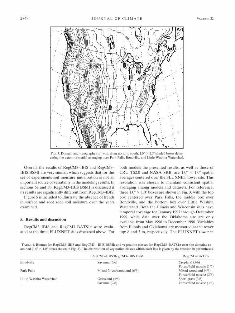
Centered at 408N, 958W, using a rotated Mercator pro-

jection, and spanning 100 points zonally and 60 points

meridionally at a horizontal grid spacing of 60 km, the

domain covers all of the United States, as well as parts of

Mexico and Canada (Fig. 3). The years simulated (1996,

1997, 1998, and 1999) were chosen for maximum overlap

with observational datasets. In all simulations presented,

the surface physics scheme was run every 600 s, or once

every three model time steps.

The 40-yr European Centre for Medium-Range

Weather Forecasts (ECMWF) Re-Analysis (ERA-40)

dataset (Uppala et al. 2005) was used to force the

boundaries under the exponential relaxation of Davies

and Turner (1977). SSTs were prescribed using the

National Oceanic and Atmospheric Administration

Optimum Interpolation SST dataset, which has a spatial

resolution of 1.08 3 1.08 and is averaged on a weekly

basis (Reynolds et al. 2002). This dataset relies on in situ

and satellite SSTs, as well as SSTs simulated from sea ice

cover (Reynolds et al. 2002). For RegCM3–IBIS, vege-

tation biomes were assigned using the potential global

vegetation dataset of Ramankutty (1999). In addition,

the following two climatology datasets were required to

populate each grid cell with PFTs: the monthly mean

climatology of temperature (New et al. 1999) and the

minimum temperature ever recorded at a location minus

the average temperature of the coldest month, created at

the University of Oregon (Bartlein 2000). In all simula-

tions presented, RegCM3–IBIS was run with static veg-

etation to create a consistent comparison among models.

Vegetation in RegCM3–BATS1e was initialized using

the Global Land Cover Characterization (GLCC) data-

set of the U.S. Geological Survey (USGS; USGS 1997).

The vegetation cover (biomes for RegCM3–IBIS and

vegetation classes for RegCM3–BATS1e) over each

point examined is provided in Table 1. Topography

for both models was given by the USGS global 30-arc

second elevation dataset (USGS 1996) aggregated to a

0.58 3 0.58 spatial resolution.

Because initialization of soil moisture has been shown

by Fischer et al. (2007) to be important in the simulation

of European heat waves, two different types of soil

moisture initialization were used in RegCM3–IBIS. In

the first RegCM3–IBIS simulation, soil moisture, soil

temperature, and soil ice were assigned using a global

0.58 3 0.58, 15-yr offline IBIS simulation starting in 1980.

The monthly mean climatology variables required to run

the offline version of IBIS are cloudiness, precipitation

rate, relative humidity, temperature, ‘‘wet’’ days per

month, wind speed at s 5 0.995, and temperature range,

which are all products of the Climate Research Unit

dataset (New et al. 1999). In the second simulation,

RegCM3–IBIS with BATS1e soil moisture initialization

(RegCM3–IBIS BSMI), the soil moisture and tempera-

ture fields at initialization were set identical to those of

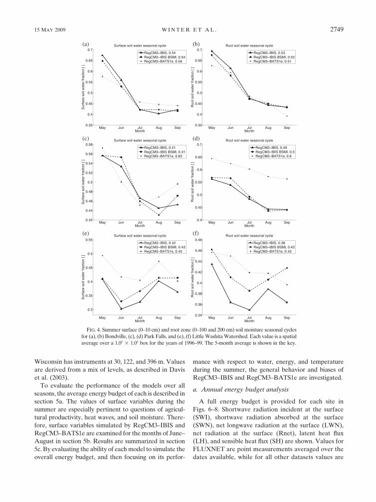
RegCM3–BATS1e. Figure 4 describes the summer sea-

sonal cycles of surface and root zone soil moisture in

RegCM3–IBIS, RegCM3–IBIS BSMI, and RegCM3–

BATS1e. Surface soil moisture is presented as the soil

water fraction of the surface soil layer, which is the same

for both models (0–10 cm). Root zone soil moisture is the

soil water fraction for the root zone soil layer, the thick-

ness of which varies in BATS1e based on vegetation type

(0–100 cm and 0–200 cm) and is fixed in IBIS (0–100 cm).

FIG. 2. Flowchart of RegCM3–IBIS, including passed variables and

their associated units.

15 MAY 2009 W I N T E R E T A L . 2747

Overall, the results of RegCM3–IBIS and RegCM3–

IBIS BSMI are very similar, which suggests that for this

set of experiments soil moisture initialization is not an

important source of variability in the modeling results. In

sections 5a and 5b, RegCM3–IBIS BSMI is discussed if

its results are significantly different from RegCM3–IBIS.

Figure 5 is included to illustrate the absence of trends

in surface and root zone soil moisture over the years

examined.

5. Results and discussion

RegCM3–IBIS and RegCM3–BATS1e were evalu-

ated at the three FLUXNET sites discussed above. For

both models the presented results, as well as those of

CRU TS2.0 and NASA SRB, are 1.08 3 1.08 spatial

averages centered over the FLUXNET tower site. This

resolution was chosen to maintain consistent spatial

averaging among models and datasets. For reference,

three 1.08 3 1.08 boxes are shown in Fig. 3, with the top

box centered over Park Falls, the middle box over

Bondville, and the bottom box over Little Washita

Watershed. Both the Illinois and Wisconsin sites have

temporal coverage for January 1997 through December

1999, while data over the Oklahoma site are only

available from May 1996 to December 1998. Variables

from Illinois and Oklahoma are measured at the tower

top: 8 and 3 m, respectively. The FLUXNET tower in

FIG. 3. Domain and topography (m) with, from north to south, 1.08 3 1.08 shaded boxes delin-

eating the extent of spatial averaging over Park Falls, Bondville, and Little Washita Watershed.

TABLE 1. Biomes for RegCM3–IBIS and RegCM3—IBIS BSMI; and vegetation classes for RegCM3–BATS1e over the domains ex-

amined (1.08 3 1.08 boxes shown in Fig. 3). The distribution of vegetation classes within each box is given by the fraction in parentheses.

RegCM3–IBIS/RegCM3–IBIS BSMI RegCM3–BATS1e

Bondville Savanna (6/6) Cropland (5/6)

— Forest/field mosaic (1/6)

Park Falls Mixed forest/woodland (6/6) Mixed woodland (4/6)

— Forest/field mosaic (2/6)

Little Washita Watershed Grassland (4/6) Short grass (3/6)

Savanna (2/6) Forest/field mosaic (3/6)


Wisconsin has instruments at 30, 122, and 396 m. Values

are derived from a mix of levels, as described in Davis

et al. (2003).

To evaluate the performance of the models over all

seasons, the average energy budget of each is described in

section 5a. The values of surface variables during the

summer are especially pertinent to questions of agricul-

tural productivity, heat waves, and soil moisture. There-

fore, surface variables simulated by RegCM3–IBIS and

RegCM3–BATS1e are examined for the months of June–

August in section 5b. Results are summarized in section

5c. By evaluating the ability of each model to simulate the

overall energy budget, and then focusing on its perfor-

mance with respect to water, energy, and temperature

during the summer, the general behavior and biases of

RegCM3–IBIS and RegCM3–BATS1e are investigated.

a. Annual energy budget analysis

A full energy budget is provided for each site in

Figs. 6–8. Shortwave radiation incident at the surface

(SWI), shortwave radiation absorbed at the surface

(SWN), net longwave radiation at the surface (LWN),

net radiation at the surface (Rnet), latent heat flux

(LH), and sensible heat flux (SH) are shown. Values for

FLUXNET are point measurements averaged over the

dates available, while for all other datasets values are

FIG. 4. Summer surface (0–10 cm) and root zone (0–100 and 200 cm) soil moisture seasonal cycles

for (a), (b) Bondville, (c), (d) Park Falls, and (e), (f) Little Washita Watershed. Each value is a spatial

average over a 1.08 3 1.08 box for the years of 1996–99. The 5-month average is shown in the key.

15 MAY 2009 W I N T E R E T A L . 2749

1.08 3 1.08 spatial averages centered over the FLUX-

NET site and averaged over 4 yr.

Shortwave radiation incident at the surface is over-

estimated by RegCM3–IBIS and RegCM3–BATS1e

when compared to NASA SRB at Illinois and Oklahoma.

Over Wisconsin, shortwave radiation incident at the

surface is correctly simulated by RegCM3–IBIS and

underestimated by RegCM3–BATS1e. However, dur-

ing the summer RegCM3–IBIS and RegCM3–BATS1e

overestimate shortwave radiation incident at the surface

for all sites. Possible causes for the overestimation of

shortwave radiation incident at the surface are consid-

ered in section 5b.

RegCM3–IBIS absorbs the most shortwave radiation

at the surface for all sites, a result of overestimated solar

radiation incident and a lower surface albedo. RegCM3–

BATS1e simulates excess shortwave radiation absorbed

at the surface compared with NASA SRB for Illinois and

Oklahoma, although the magnitude of the overestima-

tion is less than that of RegCM3–IBIS. At the Wisconsin

site, the amount of shortwave radiation absorbed at the

surface by RegCM3–BATS1e is less than that observed,

consistent with the underestimation of shortwave radi-

ation incident at the surface.

RegCM3–IBIS overestimates net longwave radiation,

a product of higher surface temperatures (discussed in

section 5b) that drive increased upward longwave ra-

diation. RegCM3–BATS1e overestimates net longwave

radiation over Oklahoma, but to a lesser extent.

Net radiation values are similar for all models/data-

sets. Over Oklahoma and Wisconsin, NASA SRB values

for net radiation are approximately 10 W m22 more than

RegCM3–IBIS and RegCM3–BATS1e. Over Illinois,

net radiation values for RegCM3–IBIS and RegCM3–

BATS1e are very similar to those of NASA SRB and are

’10 W m22 more than those of FLUXNET.

FIG. 5. 1996–99 June–August average soil moisture for Bondville (black), Park Falls (gray),

and Little Washita Watershed (white).

FIG. 6. Energy budget for Bondville. Each bar is a 4-yr average

(1996–99) of the domain contained within the 18 3 18 box centered

over Bondville, with the exception of FLUXNET, which is a point

measurement averaged over the dates available. FIG. 7. Same as Fig. 6, but for Park Falls.


RegCM3–BATS1e overestimates latent heat flux at all

sites. RegCM3–IBIS performs better, but still simulates

excess evapotranspiration compared to FLUXNET.

RegCM3–IBIS overestimates sensible heat flux

over Illinois and Wisconsin, a result of the high sur-

face temperatures simulated by the model. RegCM3–

BATS1e simulates significantly less sensible heat than

RegCM3–IBIS, and agrees reasonably well with

FLUXNET.

b. Summer surface variable analysis

Figure 9 shows the average June–August 2-m tem-

perature and precipitation biases of RegCM3–IBIS and

RegCM3–BATS1e when compared to CRU TS2.0 over

the continental United States. RegCM3–IBIS has a

large warm bias that is most intense over the midwest-

ern United States. Temperature is significantly better

simulated by RegCM3–BATS1e, although a slight warm

bias is also found over the Midwest. Precipitation is

overestimated by both RegCM3–IBIS and RegCM3–

BATS1e; however, RegCM3–IBIS appears to have

less of a wet bias. Differences between 500-mb geo-

potential heights and winds in RegCM3–IBIS and

RegCM3–BATS1e were also examined (not pictured).

No significant differences among these variables were

found.

In Figs. 10–12, the following eight variables are eval-

uated at each site: 2-m temperature, 2-m specific hu-

midity, latent heat flux, sensible heat flux, surface short-

wave incident radiation, surface shortwave absorbed

radiation, precipitation, and surface runoff. Paired in

scatterplots, these components comprise four variables

FIG. 8. Same as Fig. 6, but for Little Washita Watershed.

FIG. 9. Average 2-m temperature (8C) and precipitation (mm day21) biases for RegCM3–IBIS and RegCM3–BATS1e compared to

CRU TS2.0 for June–August of the years of 1996–99. The bias in RegCM3–IBIS precipitation over western Mexico (three white boxes) is

’ 15 mm day21.

15 MAY 2009 W I N T E R E T A L . 2751

that are important to the performance of land surface

models: the 2-m moist static energy (MSE), Bowen ra-

tio, surface albedo, and runoff ratio. The values of these

variables can be found in Table 2. Each point is a June–

August average for 1 yr, and no differentiation is made

between years. With the exception of FLUXNET data,

which are point measurements, all presented values are

1.08 3 1.08 spatial averages. The horizontal and vertical

lines are the average values over all datasets and years

for variables on the y and x axes, respectively. Note that

FLUXNET temperature and specific humidity are not

measured at 2 m as indicated by the figure labels. The

2-m MSE is defined as

MSE 5 CpT 1 Lyq 1 gz,

where Cp is the specific heat of air, T is temperature, Ly

is the latent heat of vaporization, q is specific humidity,

and z is height (assumed to be zero in this study).

For all sites, RegCM3–IBIS absorbs the most short-

wave radiation at the surface, and also receives the most

incident shortwave radiation at the surface. Compared

with NASA SRB, both variables are overestimated by

’50 W m22 over Illinois and Wisconsin, and ’25 W m22

over Oklahoma. RegCM3–BATS1e also overpredicts

absorbed and incident shortwave radiation values, on

average ’40 W m22 for the Illinois site and ’20 W m22

over Wisconsin and Oklahoma. Solar radiation at the top

of the atmosphere (Figs. 6–8) is the same for both models

and NASA SRB; therefore, the bias in shortwave inci-

dent radiation is primarily an atmospheric problem, likely

the result of a lack of absorbed and reflected radiation in

the atmospheric column. Zhang et al. (1998) concluded

that the NCAR CCM3 does not absorb sufficient

shortwave radiation in the atmosphere, creating an

overestimation of shortwave radiation incident at the

surface. Because the radiation scheme of RegCM3 is

based on CCM3, it is probable that RegCM3 also suffers

from the same bias. The underestimation of reflected

radiation could be a result of a bias in the simulated

cloud cover, an underestimation of the reflectivity of

clouds that do exist, or a combination of the two. In

RegCM3–IBIS, the overestimation of shortwave radia-

tion absorbed at the surface is exacerbated by a lower

surface albedo over Illinois and Wisconsin (Table 2).

RegCM3–BATS1e simulates substantially more evapo-

transpiration than is observed at the Illinois and Wisconsin

FLUXNET sites, on average ’40 W m22. Latent heat

FIG. 10. Comparison of (a) surface albedo components, (b) Bowen ratio components, (c)

runoff ratio components, and (d) 2-m moist static energy components for Bondville. Each point

is a June–August average for 1 yr, 1996–99 (FLUXNET, dates available). FLUXNET values

are point measurements, while all other values are spatial averages over a 1.08 3 1.08 box.


flux over Oklahoma is well simulated by RegCM3–

BATS1e. Evapotranspiration in BATS1e is a function

of potential evaporation, stomatal resistance, and aero-

dynamic resistance. The overestimation of both latent

and sensible heat fluxes indicate that RegCM3–BATS1e

likely underestimates aerodynamic resistance; however,

a low stomatal resistance is also suggested, because the

overestimation of latent heat flux far outpaces that of

the sensible heat flux and there appears to be little or no

reduction of latent heat flux during the summertime

series (not shown). The latent heat flux of RegCM3–

IBIS over Illinois is similar to that of the FLUXNET

observations. Compared to the Wisconsin FLUXNET

observations, RegCM3–IBIS overestimates latent heat

flux by ’25 W m22. Over Oklahoma the values for la-

tent heat flux are extremely variable, but, on average,

RegCM3–IBIS simulates values that are consistent with

FLUXNET observations. Interestingly, over Oklahoma,

RegCM3–IBIS BSMI does simulate ’15 W m22 more

evapotranspiration than RegCM3–IBIS. Consistent with

Fig. 4, the variability appears to be attributable to a

difference in the soil moisture content between the two

models. This reinforces the idea that RegCM3–IBIS has

tight physiological controls on evapotranspiration. For

each site, it is important to note that site-specific vege-

tative cover will influence FLUXNET values of latent

and sensible heat considerably. FLUXNET values are

point measurements over a particular vegetation cover.

RegCM3–IBIS simulates only natural vegetation, and

both models have a finite number of PFTs, so the veg-

etation contained in the 1.08 3 1.08 averaged domain

may not be identical to the vegetation at the FLUXNET

tower. Also, the type of cover present will influence the

magnitude and distribution of evapotranspiration in

time. These discrepancies are not addressed, and could

contribute to some of the differences found.

RegCM3–IBIS overestimates sensible heat flux by ’40

W m22 at all sites. In RegCM3–IBIS, sensible heat flux

is determined by a temperature difference between two

levels and a transfer coefficient. RegCM3–IBIS over-

estimates surface temperature, thus increasing the dif-

ference and significantly enhancing the sensible heat flux.

The sensible heat flux simulated by RegCM3–BATS1e

is comparable to FLUXNET over Illinois, and is ’20 W

m22 more at both the Oklahoma and Wisconsin sites.

Similar to RegCM3–IBIS, the overestimation of tem-

perature in RegCM3–BATS1e contributes to its increased

sensible heat flux. In addition, as discussed above, it is

likely that RegCM3–BATS1e underestimates aerody-

namic resistance, which would also enhance sensible heat

flux. Commensurate with the increased latent heat flux of

RegCM3–IBIS BSMI when compared to RegCM3–IBIS

over Oklahoma, on average RegCM3–IBIS BMSI sim-

ulates less sensible heat at this site, ’10 W m22.

FIG. 11. Same as Fig. 10, but for Park Falls.

15 MAY 2009 W I N T E R E T A L . 2753

Precipitation values for models and observations have

high interannual variability at all sites. Note that runoff

values are not available for FLUXNET, so precipitation

points are placed on the model/dataset average line for

convenience. Few clear trends emerge. Overall RegCM3–

BATS1e simulates more rainfall than RegCM3–IBIS.

Consistent with the greater amount of simulated rain-

fall, RegCM3–BATS1e also simulates more surface

runoff at all sites, and substantially more over Wisconsin.

Over Illinois, RegCM3–IBIS simulates slightly less rain-

fall than FLUXNET, and RegCM3–BATS1e simulates

slightly more. RegCM3–BATS1e overestimates rainfall

at the Wisconsin site when compared to FLUXNET

observations; RegCM–IBIS does not. The rainfall and

surface runoff values of RegCM3–IBIS BSMI diverge

from those of RegCM3–IBIS, suggesting that soil

moisture initialization does play an important role in

the simulation of these two variables. This is especially

evident over Wisconsin, where the rainfall of RegCM3–

IBIS BSMI is closer to RegCM3–BATS1e than

RegCM3–IBIS.

The 2-m temperature values of CRU TS2.0 and

FLUXNET generally agree for all sites. RegCM3–

BATS1e does have a slight warm bias, approximately

18C averaged across all sites. This is consistent with

overestimated shortwave radiation absorbed at the

surface in RegCM3–BATS1e and is likely moderated

by its overestimation of latent heat flux. For each site,

RegCM3–IBIS shows a clear warm bias over all of the

years evaluated, on average approximately 58C. Both

excess shortwave radiation absorbed (and incident) at

the surface and low latent heat fluxes drive the overes-

timation of temperature in RegCM3–IBIS.

RegCM3–IBIS underestimates specific humidity by

’1.5 g kg21 over Illinois and simulates excess specific

humidity (’2 g kg21) over Wisconsin compared to

FLUXNET and CRU TS2.0 observations. RegCM3–

BATS1e simulates specific humidity well at all three sites.

FLUXNET and CRU TS2.0 disagree significantly over

Oklahoma, and both have high interannual variability.

c. Summary

Over the summer, RegCM3–IBIS and RegCM3–

BATS1e absorb too much shortwave radiation at the

surface. RegCM3–BATS1e absorbs an average of ’25

W m22 more shortwave radiation at the surface than

NASA SRB. Faced with excess energy, the model must

choose how it will balance the energy budget. In

RegCM3–BATS1e, this is achieved through enhanced

latent heat flux. For all sites RegCM3–BATS1e simu-

lated more evapotranspiration than both RegCM3–

IBIS and FLUXNET.

In contrast, RegCM3–IBIS has strict physiological

controls on latent heat flux. This sensitivity of plants to

FIG. 12. Same as Fig. 10, but for Little Washita Watershed.


soil moisture results in smaller values of evapotranspi-

ration, which are closer to FLUXNET observations. By

not allowing the approximate 40 W m22 of excess en-

ergy to leave the system as latent heat flux during the

summer months, RegCM3–IBIS creates multiple other

biases, all displayed in Figs. 10–12. First, the tempera-

ture of the surface increases dramatically. Second, the

warming of the surface leads to increased sensible heat

flux and longwave radiation upward. These primary

effects cascade through the system with several possible

consequences. RegCM3–IBIS will have an earlier

snowmelt and therefore a lower annually averaged al-

bedo. Evaporation from free water surfaces will in-

crease. Given a water-limited environment, soil mois-

ture will decrease and plants will be more likely to be-

come water stressed, which will reduce precipitation

and increase the temperature further. These results are

much more dramatic than those experienced by re-

moving excess energy as latent heat. When evapo-

transpiration is enhanced, the surface does not warm

and the temperature may even decrease because of

evaporative cooling. In this case, beside a bias in latent

heat flux, no other gross observable errors exist.

6. Conclusions

The coupling of IBIS to RegCM3 is presented in this

article. In addition, RegCM3–IBIS and RegCM3–

BATS1e are evaluated with respect to the NASA SRB,

FLUXNET, and CRU TS2.0 datasets for the period of

1996–99. Three FLUXNET sites in the midwestern

United States were selected: Bondville, Illinois; Park

Falls, Wisconsin; and Little Washita Watershed, Okla-

homa. The skill of each model in simulating all facets of

the energy budget, as well as 2-m temperature, 2-m

specific humidity, precipitation, and surface runoff, was

assessed at each site.

IBIS has been successfully coupled to RegCM3. The

resulting model adds many features to RegCM3, in-

cluding dynamic vegetation, the coexistence of multiple

PFTs in the same grid cell, more sophisticated plant

phenology, plant competition, explicit modeling of soil/

plant biogeochemistry, and additional soil and snow

layers. An improved method for initializing soil mois-

ture and temperature has been implemented.

RegCM3–IBIS has a significant warm bias. Shortwave

radiation incident, shortwave radiation absorbed, net

longwave radiation, and sensible heat flux at the surface

are overestimated. Latent heat flux is well simulated by

RegCM3–IBIS, as is net radiation, surface runoff, and

precipitation. RegCM3–BATS1e contains many of the

same biases in shortwave radiation, especially during

the summer months. In contrast to RegCM3–IBIS,

RegCM3–BATS1e correctly simulates temperature,

net longwave radiation, and sensible heat flux, but

TABLE 2. Values for summer surface variables in Figs. 10–12. Each value is a June–August average for the years 1996–99 (FLUXNET:

1997–99 for Illinois and Wisconsin; 1996–98 for Oklahoma). FLUXNET values are point measurements, while all other values are spatial

averages over a 1.08 3 1.08 box.

Surface albedo Bowen ratio Runoff ratio 2m MSE (J kg21)

Bondville

RegCM3–IBIS 0.14 0.78 0.23 3.36E 1 05

RegCM3–IBIS BSMI 0.14 0.78 0.22 3.35E 1 05

RegCM3–BATS1e 0.18 0.26 0.18 3.35E 1 05

NASA SRB 0.17 — — —

CRU TS2.0 — — — 3.32E 1 05

FLUXNET — 0.23 — 3.35E 1 05

Park Falls

RegCM3–IBIS 0.13 0.69 0.02 3.31E 1 05

RegCM3–IBIS BSMI 0.13 0.68 0.08 3.31E 1 05

RegCM3–BATS1e 0.14 0.33 0.17 3.24E 1 05

NASA SRB 0.15 — — —

CRU TS2.0 — — — 3.20E 1 05

FLUXNET — 0.23 — 3.20E 1 05

Little Washita Watershed

RegCM3–IBIS 0.16 1.34 0.16 3.41E 1 05

RegCM3–IBIS BSMI 0.16 0.90 0.12 3.41E 1 05

RegCM3–BATS1e 0.14 0.93 0.13 3.40E 1 05

NASA SRB 0.16 — — —

CRU TS2.0 — — — 3.40E 1 05

FLUXNET — 0.65 — 3.43E 1 05

15 MAY 2009 W I N T E R E T A L . 2755

systematically overestimates latent heat flux. RegCM3-

IBIS and RegCM3-BATS1e different tendencies of

models when faced with excessive radiation, a question

that is particularly salient when attempting to assess the

effects of changes in the radiative forcing.

To improve RegCM3–IBIS, the simulation of short-

wave absorbed radiation must be corrected. This includes

addressing the bias in shortwave incident radiation in the

atmospheric components of RegCM3 and the underes-

timation of albedo in IBIS. To help correct the over-

estimation of surface temperature and sensible heat

flux, the limitations on latent heat flux during the sum-

mer should be relaxed. Finally, anthropogenic land use

biomes should be included in the model to better rep-

resent the current vegetation cover of the Midwest.

Acknowledgments. We thank the International Cen-

tre for Theoretical Physics, the Eltahir Group, members

of the Ralph M. Parsons Laboratory who aided in this

research, our reviewers, and our editor. Individuals

who made significant contributions to this work include

Filippo Giorgi and Marc Marcella. This work was fun-

ded by the National Science Foundation (Award EAR-

04500341), the Linden Fellowship, and the International

Centre for Theoretical Physics.

REFERENCES

Anthes, R., 1977: A cumulus parameterization scheme utilizing a

one-dimensional cloud model. Mon. Wea. Rev., 105, 270–286.

——, E. Hsie, and Y.-H. Kuo, 1987: Description of the Penn State/

NCAR Mesoscale Model Version 4 (MM4). NCAR Tech.

Note NCAR/TN-2821STR, 79 pp.

Baldocchi, D., and Coauthors, 2001: FLUXNET: A new tool to

study the temporal and spatial variability of ecosystem-scale

carbon dioxide, water vapor, and energy flux densities. Bull.

Amer. Meteor. Soc., 82, 2415–2434.

Ball, J., I. Woodrow, and J. Berry, 1986: A model predicting sto-

matal conductance and its contribution to the control of

photosynthesis under different environmental conditions.

Proc. Seventh Int. Congress on Photosynthesis, Providence,

RI, 221–224.

Bartlein, P., 2000: Absolute minimum temperature minus average

of the coldest monthly mean temperature Worldwide Airfield

Summaries. [Available online at http://www.sage.wisc.edu/

download/IBIS.]

Claassen, M. M., and R. Shaw, 1970: Water deficit effects on corn.

I. Vegetative components. Agron. J., 62, 649–652.

Davies, H., and R. Turner, 1977: Updating prediction models by

dynamical relaxation: An examination of the technique.

Quart. J. Roy. Meteor. Soc., 103, 225–245.

Davis, K., P. Bakwin, C. Yi, B. Berger, C. Zhao, R. Teclaw, and J.

Isebrands, 2003: The annual cycles of CO2 and H2O exchange

over a northern mixed forest as observed from a very tall

tower. Global Change Biol., 9, 1278–1293.

Delire, C., S. Levis, G. Bonan, J. A. Foley, M. T. Coe, and S.

Vavrus, 2002: Comparison of the climate simulated by the

CCM3 coupled to two different land-surface models. Climate

Dyn., 19, 657–669.

Dickinson, R. E., R. M. Errico, F. Giorgi, and G. T. Bates, 1989: A

regional climate model for the western United States. Cli-

matic Change, 15, 383–422.

——, A. Henderson-Sellers, and P. J. Kennedy, 1993: Biosphere

Atmosphere Transfer Scheme (BATS) version 1e as coupled

to the NCAR Community Climate Model. NCAR Tech. Note

NCAR/TN-3871STR, 80 pp.

Eastman, J., M. Coughenour, and R. Pielke Sr., 2001: The regional

effects of CO2 and landscape change using a coupled plant

and meteorological model. Global Change Biol., 7, 797–815.

Eltahir, E. A. B., and R. L. Bras, 1994: Sensitivity of regional cli-

mate to deforestation in the Amazon basin. Adv. Water Res.,

17, 101–115.

Emanuel, K. A., 1991: A scheme for representing cumulus con-

vection in large-scale models. J. Atmos. Sci., 48, 2313–2329.

Falge, E., and Coauthors, 2005: FLUXNET Marconi conference

gap-filled flux and meteorology data, 1992-2000. [Available

online at http://daac.ornl.gov/FLUXNET/guides/marconi_

gap_filled.html.]

Farquhar, G. D., and T. D. Sharkey, 1982: Stomatal conductance

and photosynthesis. Annu. Rev. Plant Physiol., 33, 317–345.

——, S. von Caemmerer, and J. A. Berry, 1980: A biogeochemical

model of photo synthetic CO2 assimilation in leaves of C3

species. Planta, 149, 78–90.

Fischer, E. M., S. I. Seneviratne, P. L. Vidale, D. Luthi, and C.

Schar, 2007: Soil moisture–atmosphere interactions during the

2003 European summer heat wave. J. Climate, 20, 5081–5099.

Foley, J., I. Prentice, N. Ramankutty, S. Levis, D. Pollard, S. Sitch,

and A. Haxeltine, 1996: An integrated biosphere model of

land surface processes, terrestrial carbon balance, and vege-

tation dynamics. Global Biogeochem. Cycles, 10, 603–628.

Friend, A., 1995: PGEN: An integrated model of leaf photosyn-

thesis, transpiration, and conductance. Ecol. Modell., 77,

233–255.

Giorgi, F., 1990: Simulation of regional climate using a limited area

model nested in a general circulation model. J. Climate, 3,

941–963.

——, and G. Bates, 1989: The climatological skill of a regional

model over complex terrain. Mon. Wea. Rev., 117, 2325–

2347.

Grell, G. A., 1993: Prognostic evaluation of assumptions used by

cumulus parameterizations. Mon. Wea. Rev., 121, 764–787.

Holtslag, A. A. M., E. I. F. de Bruijn, and H.-L. Pan, 1990: A high

resolution air mass transformation model for short-range

weather forecasting. Mon. Wea. Rev., 118, 1561–1575.

Kiehl, J. T., J. J. Hack, G. B. Bonan, B. A. Boville, B. P. Breigleb,

D. L. Williamson, and P. J. Rasch, 1996: Description of the

NCAR Community Climate Model (CCM3). NCAR Tech.

Note NCAR/TN-4201STR, 159 pp.

King, S. S., 1981: Down on the farm, higher prices. New York

Times, 11 January, Section 12, 01.

Kumar, S. V., C. D. Peters-Lidard, J. L. Eastman, and W.-K. Tao,

2008: An integrated high-resolution hydrometeorological

modeling testbed using LIS and WRF. Environ. Modell.

Software, 23, 169–181.

Leuning, R., 1995: A critical appraisal of a combined stomatal-

photosynthesis model for C3 plants. Plant Cell Environ., 18,

339–355.

Lloyd, J., 1991: Modelling stomatal responses to environment in

Macadamia integrifolia. Aust. J. Plant Physiol., 18, 649–660.

——, and G. Farquhar, 1994: 13C discrimination during CO2

assimilation by the terrestrial biosphere. Oecologia, 99,

201–215.


Lynch, A. H., W. Wu, G. Bonan, and F. Chapin III, 1999: The

impact of tundra ecosystems on the surface energy budget and

climate of Alaska. J. Geophys. Res., 104, 6647–6660.

Mitchell, T. D., T. R. Carter, P. D. Jones, M. Hulme, and M. New,

2004: A comprehensive set of high-resolution grids of monthly

climate for Europe and the globe: The observed record (1901–

2000) and 16 scenarios (2001–2100). Tyndall Centre for Cli-

mate Change Research Working Paper 30. [Available online

at http://www.tyndall.ac.uk/publications/working_papers/wp55.

pdf.]

New, M., M. Hulme, and P. Jones, 1999: Representing twentieth-

century space–time climate variability. Part I: Development

of a 1961–90 mean monthly terrestrial climatology. J. Climate,

12, 829–856.

Pal, J. S., E. E. Small, and E. A. B. Eltahir, 2000: Simulation

of regional-scale water and energy budgets: Representation

of subgrid cloud and precipitation processes within RegCM.

J. Geophys. Res., 105, 29 579–29 594.

——, and Coauthors, 2007: Regional climate modeling for the

developing world: The ICTP RegCM3 and RegCNET. Bull.

Amer. Meteor. Soc., 88, 1395–1409.

Pollard, D., and S. L. Thompson, 1995: Use of a land-surface-

transfer scheme (LSX) in a global climate model: The re-

sponse to doubling stomatal resistance. Global Planet. Change,

10, 129–161.

Ramankutty, N., 1999: Estimating historical changes in land cover:

North American croplands from 1850 to 1992. Global Ecol.

Biogeogr., 8, 381–396.

Reynolds, R. W., N. A. Rayner, T. M. Smith, D. C. Stokes, and W.

Wang, 2002: An improved in situ and satellite SST analysis for

climate. J. Climate, 15, 1609–1625.

Thom, A. S., and H. R. Oliver, 1977: On Penman’s equation for

estimating regional evaporation. Quart. J. Roy. Meteor. Soc.,

103, 345–357.

Thompson, S. L., and D. Pollard, 1995a: A global climate model

(GENESIS) with a land-surface transfer scheme (LSX). Part

I: Present climate simulation. J. Climate, 8, 732–761.

——, and ——, 1995b: A global climate model (GENESIS) with a

land-surface transfer scheme (LSX). Part II: CO2 sensitivity.

J. Climate, 8, 1104–1121.

Twine, T. E., and Coauthors, 2000: Correcting eddy-covariance flux

underestimates over a grassland. Agric. For. Meteor., 103, 279–300.

Uppala, S. M., and Coauthors, 2005: The ERA-40 Re-Analysis.

Quart. J. Roy. Meteor. Soc., 131, 2961–3012.

USGS, cited 1996: Global 30-arc second elevation dataset

(GTOPO30). [Available online at http://edc.usgs.gov/products/

elevation/gtopo30/gtopo30.html.]

——, cited 1997: Global land cover characterization. [Available

online at http://edc2.usgs.gov/glcc/.]

Zeng, X., M. Zhao, and R. E. Dickinson, 1998: Intercomparison of

bulk aerodynamic algorithms for the computation of sea sur-

face fluxes using TOGA COARE and TAO data. J. Climate,

11, 2628–2644.

Zhang, M. H., W. Y. Lin, and J. T. Kiehl, 1998: Bias of atmospheric

shortwave absorption in the NCAR Community Climate

Models 2 and 3: Comparison with monthly ERBE/GEBA

measurements. J. Geophys. Res., 103, 8919–8925.

15 MAY 2009 W I N T E R E T A L . 2757

Coupling of Integrated Biosphere Simulator to Regional ...

Documents

Transcript of Coupling of Integrated Biosphere Simulator to Regional ...