COUPLE’S BEHAVIOUR IN THE BRAZILIAN LABOUR MARKET … · COUPLE’S BEHAVIOUR IN THE BRAZILIAN...

April, 2013Working Paper number 107

COUPLE’S BEHAVIOUR INTHE BRAZILIAN LABOUR MARKET:

THE INFLUENCE OF SOCIAL SECURITY AND INDIVIDUALCHARACTERISTICS ON MARRIED INDIVIDUALS’LABOUR SUPPLY DECISIONS

International

Centre for Inclusive Growth

Bernardo Lanza QueirozDepartment of Demography and Cedeplar, UFMG

Laetícia Rodrigues de SouzaCenter for Demography and Ecology, University of Wisconsin-Madison andInternational Policy Centre for Inclusive Growth (IPC-IG)

Copyright© 2013International Policy Centre for Inclusive GrowthUnited Nations Development Programme

The International Policy Centre for Inclusive Growth is jointly supported by the Poverty Practice,Bureau for Development Policy, UNDP and the Government of Brazil.

Rights and Permissions

All rights reserved.

The text and data in this publication may be reproduced as long as the source is cited.Reproductions for commercial purposes are forbidden.

International Policy Centre for Inclusive Growth (IPC - IG)Poverty Practice, Bureau for Development Policy, UNDP

Esplanada dos Ministérios, Bloco O, 7º andar

70052-900 Brasilia, DF - BrazilTelephone: +55 61 2105 5000

E-mail: [email protected] URL: www.ipc-undp.org

The International Policy Centre for Inclusive Growth disseminates the findings of its work inprogress to encourage the exchange of ideas about development issues. The papers aresigned by the authors and should be cited accordingly. The findings, interpretations, andconclusions that they express are those of the authors and not necessarily those of theUnited Nations Development Programme or the Government of Brazil.

Working Papers are available online at www.ipc-undp.org and subscriptions can be requestedby email to [email protected]

Print ISSN: 1812-108X

COUPLE’S BEHAVIOUR IN THE BRAZILIAN LABOUR MARKET:

THE INFLUENCE OF SOCIAL SECURITY AND INDIVIDUAL CHARACTERISTICS ON MARRIED INDIVIDUALS’ LABOUR SUPPLY DECISIONS

Bernardo Lanza Queiroz and Laetícia Rodrigues de Souza*

ABSTRACT

In recent years, a large number of studies have investigated the relationship between social security benefits and male retirement decisions in developed countries. However, women’s and couples’ labour supply decisions and the patterns of withdrawal from the labour force in emerging economies are much less studied. This paper uses Brazilian data from 1998 to 2008 to examine how social security financial incentives and personal characteristics affects one’s own and spouses’ retirement decisions. Our results suggested that couples synchronize retirement and that they respond similarly to their own characteristics. We also find that wives are more responsive to husbands’ incentives than vice-versa.

Keywords: labour supply decisions, retirement, social security, couples, Brazil

1 INTRODUCTION

The ageing of the population increases the concern for the sustainability of public social support programs for the elderly (Wise, 2004; 2010; Bloom and McNikkon, 2010). If in the past a large part of the support for the elderly was provided by the family, today this support comes from programs created by the public sector and, in some countries, also by the private sector (Costa, 1998; Gruber and Wise, 1999; 2004).

* Bernardo Lanza Queiroz, Department of Demography and Cedeplar, UFMG. Financial support from the Fundação de Amparo a Pesquisa de Minas Gerais (Fapemig) and Conselho Nacional de Pesquisa (CNPq) is gratefully acknowledged (PPM-00542-11). Email: [email protected] and Laetícia Rodrigues de Souza, Center for Demography and Ecology, University of Wisconsin-Madison and International Policy Centre for Inclusive Growth (IPC-IG). Financial support from the Fogarty Foundation is gratefully acknowledged. Email: [email protected].

2 International Policy Centre for Inclusive Growth

However, recently, the vast majority of programs have come up against serious fiscal and financial problems (Bongaarts, 2004; Gruber and Wise, 2004). The balance of the programs is increasingly difficult to manage with an increase in the ratio of dependence, population ageing and a faster process of reducing the average retirement age (Bongaarts, 2004; Bloom and McNikkon, 2010; Mason, Lee and Lee, 2010; Wise, 2010).

Brazil is one of the countries facing such problems. Despite unabated interest among researchers in issues pertaining to the impacts of population ageing and economic development on the sustainability of social security in developed countries (Gruber and Wise, 1988; 2004; 2008; Wise, 2010), little is known about trends in the labour force of the elderly in in emerging economies (Queiroz, 2007; 2008; Carvalho-Filho, 2008; Soares, 2010; Aguila, 2012). Brazil is one example of an important context for elaborating linkages between population ageing, public pension systems and labour force participation of older individuals. The rapid ageing population presents one of the greatest public policy challenges in Brazil. At the same time, the length of working life has fallen over time, which results from both increases in educational attainment (younger workers) and changes in retirement behaviour (older workers). The fall in economic participation for older workers (65 and older) is striking: 22.3 per cent of them were in the labour force in 2010 compared to 60 per cent in 1970. In 2005, social security benefits and other forms of support for the elderly represented about 14 per cent of GDP (Ansileiro and Paiva, 2008) and are expected to be the fastest growing component of public spending (Giambiagi and Além, 1997; Giambiagi and Castro, 2003; Soares, 2010).

A second related question is how the provision of social security benefits affects older workers’ labour supply decisions (Wise, 2004). This paper builds on the preliminary analysis developed by Queiroz (2006) using data from the 1998 Brazilian Household Survey (Pesquisa Nacional por Amostra de Domicilios – PNAD) to further investigate the behaviour of couples in the Brazilian labour market. The literature on male retirement behaviour is extensive (Lazear, 1986; Lumsdaine and Mitchell, 1999). People know a great deal about male labour force participation in different countries around the world. The knowledge on female and couple’s labour supply decisions and retirement behaviour is less developed. However, the increasing female labour force participation implies that they are also an important part of the retirement decision and social security problem. Because of data limitation, very few empirical studies exist on this topic (Blau, 1998; Maestas, 2001; Coile, 2004, among others). This paper contributes to this field by estimating the determinants of couples’ joint labour supply decisions in a developing economy.

Male retirement studies assume a simple framework focusing on economic considerations as the main explanatory variable. The basic idea of these models is that workers will evaluate the gains (or losses) of leaving the labour force and retiring now compared to working one more year before deciding to leave or stay in the labour market (Gruber and Wise, 1999; 2004). However, whether one member of the household retires, or is deciding to do so, affects the socio-economic situation of the family and of his/her partner. Therefore, family variables should also be taken into account.

One question of interest might be how one's spouse's retirement decision affects the behavior of the other spouse. One possible outcome is that couples decide to withdraw from the labour force at the same time. Several reasons explain this outcome:

Working Paper 3

1. share leisure time together. Spouses would like to have mortime with each other in older age after leaving the labour force and not having kids at home;

2. item couples share similar tastes, as a result of assortative mating one can expect that couples have similar career paths and/or working behavior;

3. financial incentives, social security wealth, and other economic reasons.

In particular, we use PNAD data to estimate the effect of each spouse’s characteristics and public pension incentives on their own and their partner’s probabilities of staying or leaving the labour market. The aim is to explore whether couples synchronize their retirement; the effect of one spouse’s incentives/variables on the other spouse’s decision; and the possible implications of changes in the rules governing social security benefits in Brazil.

The paper contributes to the empirical literature by analysing couples’ and women’s labour supply and retirement in Brazil. The contribution is twofold: first, it studies social security incentives in a developing country with a large public pension system and rapid ageing population. Second, it analyses a system with different rules for males and females, which is not the case of the USA. In addition to that, it provides empirical results in a time of intense debate over changes in the Brazilian system. Therefore, it also aims to provide support for policymakers by investigating possible impacts of legislation changes on retirement.

In Brazil, as is the case of many European countries, the normal retirement age and time of contribution to the social security system is shorter for women than for men. The normal age of retirement for women is 60 years and for men is 65. If retiring by length of contribution, women need to prove 30 years of working life, whereas men need to prove 35 years.

In recent years, European countries have faced continuous debate over the validity of such rules. The political argument is that such rules do not meet basic principles of equal treatment. Interestingly, in the beginning of the debate the main reason for change came from the political side. Only later on did the possible economic impacts of legislation change become relevant to the debate. In the 2000s, all Organisation for Economic Co-operation and Development (OECD) countries have the same retirement age for both sexes, except Italy, where women can retire five years before men.

One of the propositions to the current debate on social security change in Brazil is to equalise the rules for men and women. The premise is that equalising requirements would lead to a higher average retirement age for women. It is important, however, to measure the impact of such change, since it may also have implications on male retirement age.

There are several important findings in the paper. First, we have evidence that the social security system in Brazil creates incentives to start collecting pension benefits when possible and leaving the labour force early and that they are more beneficial to the better-off sub-population groups. Second, we observe that males and females respond in the same way to their own characteristics (specifically, age and education). Third, and more interesting, we find that husbands and wives react differently to their spouse’s variables. In particular, we find that husbands respond positively to wives’ education, which measures wealth and income, but the opposite effect is negative. Fourth, we observe that the effects of health status changed from 1998 to 2008, but it is necessary to further investigate the results.


2 EVIDENCE OF COUPLE’S LABOUR SUPPLY DECISIONS

Empirical research on retirement and labour supply decisions of couples and married women is not very common. Bowen and Finegan (1969) estimate a model using the 1960 US Census and find that older wives work less when husbands are retired and in households with high income. Henretta and O’Rand (1983) present a more sophisticated model, using the Retirement and History Survey. They estimate logistic regression models comparing the joint retirement decisions to when one spouse retires before the other. They find that economic and non-economic variables influence wives’ retirement. Pozzenbon and Mitchell (1989) developed a model to examine the economic and family determinants of retirement among married women. The results show that wives do not respond to changes in social security wealth. However, familial determinants, husband’s health and leisure time are the main determinants of married women’s retirement behaviour. The previous studies focused on a descriptive and empirical analysis of the problem. More recent research has incorporated economic models to consider couples’ utility when studying the process. Hurd (1990) studies couples’ retirement dates using a sample from the New Beneficiary Survey. He observes that couples retire within a short period of time, as about 30 per cent of couples retire within a year of each other. Hurd estimates two separate regression models, one for males and one for females, and finds that increasing the wife’s retirement age by 1 year increases her husband’s retirement age by 0.25 years, and increasing the husband’s retirement age by 1 year increases his wife’s retirement age by 0.37 years. Blau (1998) and Gustman and Steinmeier (2000) developed structural econometric models to study the issue of joint retirement. The results indicate a coincidence of retirement dates, even when the wife is much younger than her husband. The main explanation for such behaviour in these studies is similar tastes for leisure. The authors show that economic variables and financial incentives are not the only explanation for the high incidence of joint retirement. Maestas (2001) develops a structural model to determine joint retirement decisions using data from the Health and Retirement Survey (HRS). Her results go in the same direction as previous studies, supporting the idea that couples with greater leisure tend to retire together.

Zweimuller, Winter-Ebmer and Falkinger (1996) analysed the impact of changes in the minimum retirement age in Austria on couples’ retirement decisions. The results confirm the existence of joint leisure preferences. However, the results also indicate that financial and economic variables are relevant and that the impact of changes in retirement age is stronger on wives’ than on husbands’ decisions. Coile (2004) argues that the literature has not addressed two important aspects of joint retirement decisions: the effect of women’s retirement financial incentives on the couples’ decision and the spillover effects of an individual’s financial incentives on his/her spouse’s decision. She finds that both are equally responsive to their own financial incentives and that men are more responsive to their wives’ incentives than the other way around.

In the case of Brazil, and other emerging economies, very few studies have tried to understand retirement behaviour for either females or couples. Legrand (1995), Queiroz (2007; 2008), Carvalho-Filho (2008) and Soares (2010) are the only studies on retirement in Brazil. In common, all the papers concentrate on male retirement and do not include female labour supply or familial incentives. At a time of intense debate on social security changes, it is fundamental to understand what determines retirement in Brazil and how possible changes would affect this behaviour.

Working Paper 5

3 DATA

We use data from the PNAD 1998, 2003 and 2008. PNAD is a nationally representative stratified random sample of the Brazilian population that comprises about 90,000 households. The survey consists of cross-sections collected annually since 1971, except in 1994 and during census years (1980, 1991, 2000 and 2010). The PNAD contains a comprehensive and comparable set of demographic and economic variables, including detailed information on economic activities, contribution for social security programs and whether individuals receive benefits. In this paper, we concentrate the analysis on the 1998, 2003 and 2008 data to take advantage of their health supplement.

Data limitation prevents us from examining different types of social security benefits. We can only know if the respondent is receiving retirement or survival benefits. We do not know whether the retirement is due to old age, length of contribution, disability or social assistance. In addition, we do not know whether the respondent is enrolled in the general system or civil servants programs. We, partially, solve this problem by looking at the individual’s previous occupation and her/his status in the labour force. Carvalho-Filho (2008) uses a similar approach. We do not believe this limitation affects our conclusions.

3.1 SUMMARY STATISTICS AND PRELIMINARY EVIDENCE

We construct our sample by selecting married couples (formal and informal unions) living in urban areas between the ages of 45 and 70.1 We further restrict the sample to couples who were retired or still in the labour force in the week of reference, resulting in 13,172 couples in 1998, 16,349 in 2003 and 19,024 in 2008. The couple’s mean age differential is 3.23 years (St. Dev. 6.82) and around 80 per cent of the women were married to men of the same age or older in the three years. Spouses share similar observed characteristics, such as education and race.2

Summary statistics are presented in Table 1. In our 1998 sample, men and women are, on average, 56.83 and 53.6 years old, respectively, which does not change over the period. Although showing evidence of an increase in the educational levels in Brazil, they are still very low, especially for older cohorts. Couples analysed in 1998 have completed, on average, 6.35 years of education. In 1998 (2008), 43.73 per cent (35.03 per cent) of males and 17.17 per cent (16.34 per cent) of females received pension benefits (i.e. were retired). If one compares this number with the percentage in the labour force, the sum is not 100 per cent because some individuals remain in the labour force after being granted benefits. Also, for some women discontinuity in their working history affects the possibility of receiving a pension benefit. In 1998, 42.46 per cent of men and 47.30 per cent of women declared themselves as having fair or bad health. The percentage of individuals in fair/bad health decreased, especially for women, reaching 41.05 per cent for men and 42.51 per cent for women in 2008. There are three main changes in 2008 compared to 1998. Couples’ average years of formal schooling increased from 6.35 to about 7.63 years, female labour force participation increased from 39 per cent to 49 per cent, and the percentage of husbands retired declined from 44 per cent to 35 per cent.

In the week of reference, 38.56 per cent of women and 70.95 per cent of men were in the labour force in 1998, whereas these figures increase (especially for women) to 48.65 per cent and 73.21 per cent, respectively, in 2008.


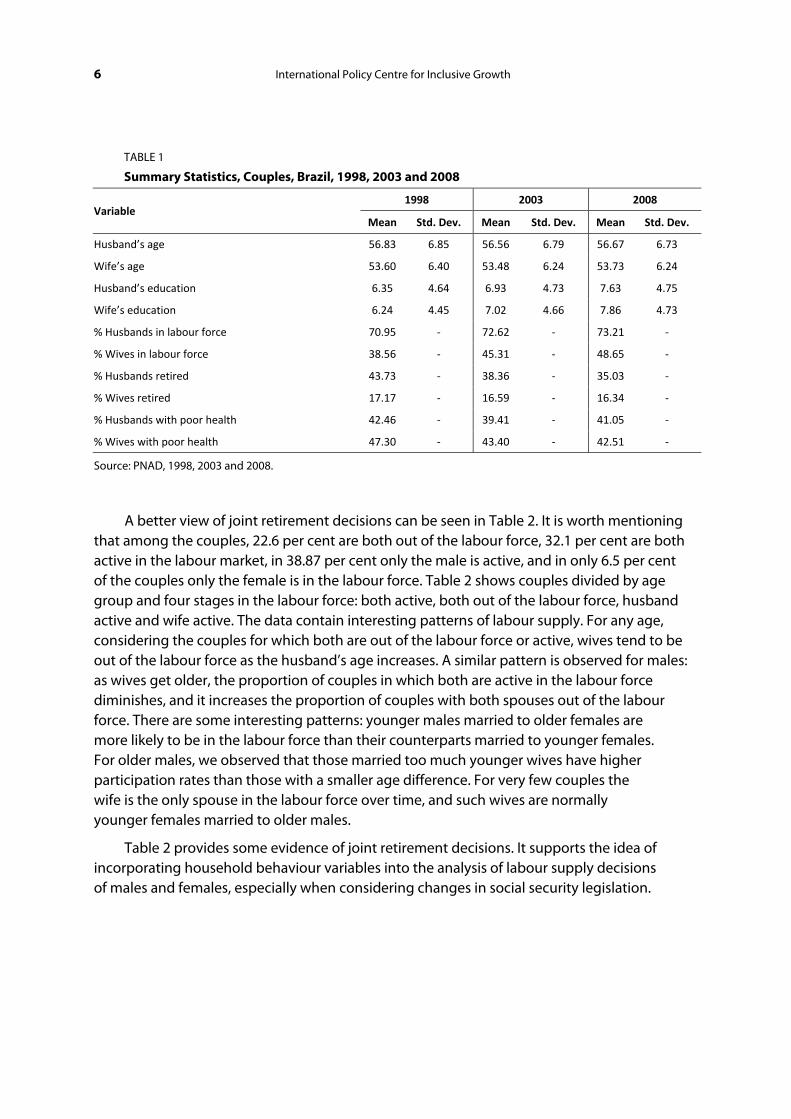
TABLE 1

Summary Statistics, Couples, Brazil, 1998, 2003 and 2008

Variable 1998 2003 2008

Mean Std. Dev. Mean Std. Dev. Mean Std. Dev.

Husband’s age 56.83 6.85 56.56 6.79 56.67 6.73

Wife’s age 53.60 6.40 53.48 6.24 53.73 6.24

Husband’s education 6.35 4.64 6.93 4.73 7.63 4.75

Wife’s education 6.24 4.45 7.02 4.66 7.86 4.73

% Husbands in labour force 70.95 ‐ 72.62 ‐ 73.21 ‐

% Wives in labour force 38.56 ‐ 45.31 ‐ 48.65 ‐

% Husbands retired 43.73 ‐ 38.36 ‐ 35.03 ‐

% Wives retired 17.17 ‐ 16.59 ‐ 16.34 ‐

% Husbands with poor health 42.46 ‐ 39.41 ‐ 41.05 ‐

% Wives with poor health 47.30 ‐ 43.40 ‐ 42.51 ‐

Source: PNAD, 1998, 2003 and 2008.

A better view of joint retirement decisions can be seen in Table 2. It is worth mentioning that among the couples, 22.6 per cent are both out of the labour force, 32.1 per cent are both active in the labour market, in 38.87 per cent only the male is active, and in only 6.5 per cent of the couples only the female is in the labour force. Table 2 shows couples divided by age group and four stages in the labour force: both active, both out of the labour force, husband active and wife active. The data contain interesting patterns of labour supply. For any age, considering the couples for which both are out of the labour force or active, wives tend to be out of the labour force as the husband’s age increases. A similar pattern is observed for males: as wives get older, the proportion of couples in which both are active in the labour force diminishes, and it increases the proportion of couples with both spouses out of the labour force. There are some interesting patterns: younger males married to older females are more likely to be in the labour force than their counterparts married to younger females. For older males, we observed that those married too much younger wives have higher participation rates than those with a smaller age difference. For very few couples the wife is the only spouse in the labour force over time, and such wives are normally younger females married to older males.

Table 2 provides some evidence of joint retirement decisions. It supports the idea of incorporating household behaviour variables into the analysis of labour supply decisions of males and females, especially when considering changes in social security legislation.

Working Paper 7

TABLE 2

Retirement Patterns of Married Couples, Brazil, 1998, 2003 and 2008

Wife’s age

Husband’s age

1998 2003 2008

Both active

Husband active

Wife active

Both retired

Both active

Husband active

Wife active

Both retired

Both active

Husband active

Wife active

Both retired

50–54

50–54 37.49 45.91 4.89 11.71 45.91 38.34 6.30 9.45 47.57 37.39 6.99 8.05

55–59 33.64 39.32 7.91 19.13 39.17 35.76 8.09 16.98 41.97 33.88 10.74 13.40

60–64 28.28 36.68 10.45 24.59 34.44 32.06 12.38 21.11 35.62 27.18 14.12 23.09

65–70 17.59 30.15 19.10 33.17 25.21 21.37 21.37 32.05 21.58 25.00 23.97 29.45

55–59

50–54 35.94 42.97 6.25 14.84 37.64 43.96 6.04 12.36 45.82 40.24 5.58 8.37

55–59 27.48 44.48 6.08 21.96 32.37 40.65 7.53 19.44 36.73 37.40 8.40 17.47

60–64 22.64 36.08 8.45 32.83 27.85 34.75 9.99 27.41 29.14 31.94 12.75 26.18

65–70 19.10 26.61 10.94 43.35 21.63 24.29 12.65 41.43 22.16 21.06 17.03 39.74

60–64

50–54 26.23 57.38 0.00 16.39 22.34 59.57 4.26 13.83 25.60 53.60 6.40 14.40

55–59 19.15 44.68 7.45 28.19 31.34 40.09 6.45 22.12 30.82 43.20 5.14 20.85

60–64 19.33 41.00 4.39 35.29 20.33 36.24 6.31 37.12 20.51 38.14 9.40 31.94

65–70 11.71 29.84 7.03 51.42 15.25 25.12 8.28 51.35 15.98 26.90 11.35 45.76

65–70

50–54 12.50 66.67 4.17 16.67 24.00 40.00 0.00 36.00 23.53 61.76 0.00 14.71

55–59 14.58 47.92 2.08 35.42 17.74 51.61 1.61 29.03 18.18 51.52 6.06 24.24

60–64 12.94 40.00 2.35 44.71 11.04 35.58 3.68 49.69 14.36 41.58 9.41 34.65

65–70 7.98 27.91 4.29 59.82 11.73 27.19 6.31 54.77 11.05 26.22 6.61 56.12

Source: PNAD, 1998, 2003 and 2008.

3.2 AGE PROFILES OF JOINT RETIREMENT

Figure 1 shows husbands’ and wives’ labour force participation rates by age (Panel A and B, respectively) in 2008. We show only the most recent year for two reasons: first, it allows us the same interpretations; second, because of space limitations. The age profile for males is very standard, as labour force participation rates decline with age. As opposed to what is observed in several developed countries, in Brazil there is no sharp decline between ages 62 and 65, the early and normal ages of retirement in the USA and European countries. The possibility of retiring by length of contribution at younger ages explains the non-existence of a clear peak. In addition, workers can stay in the labour force and receive pension benefits without penalty. For females, we observe lower (but increasing over time) labour force participation rates and faster increases at younger ages than it is observed for males. Panel B shows that more than 50 per cent of wives aged around 53 are already out of the labour force. Husbands (Panel A) reach this percentage at much older ages (around 65).


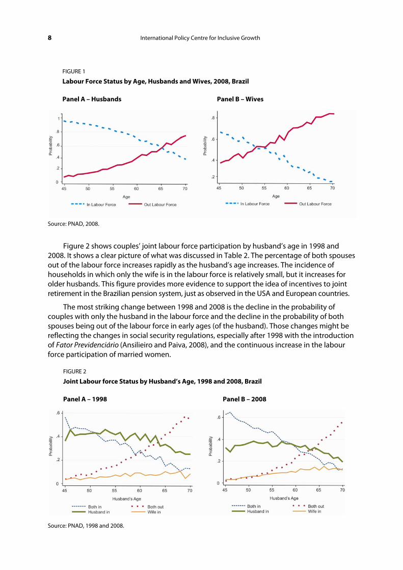
FIGURE 1

Labour Force Status by Age, Husbands and Wives, 2008, Brazil Panel A – Husbands Panel B – Wives

Source: PNAD, 2008.

Figure 2 shows couples’ joint labour force participation by husband’s age in 1998 and 2008. It shows a clear picture of what was discussed in Table 2. The percentage of both spouses out of the labour force increases rapidly as the husband’s age increases. The incidence of households in which only the wife is in the labour force is relatively small, but it increases for older husbands. This figure provides more evidence to support the idea of incentives to joint retirement in the Brazilian pension system, just as observed in the USA and European countries.

The most striking change between 1998 and 2008 is the decline in the probability of couples with only the husband in the labour force and the decline in the probability of both spouses being out of the labour force in early ages (of the husband). Those changes might be reflecting the changes in social security regulations, especially after 1998 with the introduction of Fator Previdenciário (Ansilieiro and Paiva, 2008), and the continuous increase in the labour force participation of married women.

FIGURE 2

Joint Labour force Status by Husband’s Age, 1998 and 2008, Brazil Panel A – 1998 Panel B – 2008

Source: PNAD, 1998 and 2008.

Working Paper 9

4 METHODOLOGY

We estimate retirement hazard rates from the data in two ways. First, we calculate stocks of couples in and out of the labour force in the period of analysis, and then we estimate the risk of retiring between ages and other characteristics. Second, we use information from questions regarding labour force during the year preceding the survey and the survey’s reference week to measure retirement flows. PNAD asks respondents whether they were employed during the week preceding the interview and, if not, whether they worked during the preceding year. We use this strategy because individuals could be receiving pension benefits and still remain in the workforce in Brazil. Giatti and Barreto (2003) estimate that about 25 per cent of older persons collecting pension benefits are still active in the labour market.

It is important to distinguish the main impacts on retirement stock and flow. The first is a function of cumulative impact of past age and period effects (such as earning history, health, work conditions), whereas the latter is more strongly influenced by short-term events. The main problem of analysing retirement flows using only one year of data is that we are also capturing period effects. For instance, retirement might have been particularly low or high in that year, which might affect the results. In this paper, we estimate retirement risks using both the stock and flow approaches, using all possible variables that exist for individuals in and out of the labour force, and the results are presented and briefly compared.

4.1 ESTIMATION PROCEDURES

In addition to providing the previous descriptive analysis of the samples and a graphical analysis of couple’s labour supply decision behaviour we use a bivariate probit model.

Equation 1 represents men’s probability of being out of the labour force and Equation 2 represents women’s probability. They represent the general bivariate probit model, where Probit(pm) (Probit(pf)) – represents the men’s (women’s) probability of being out of the labour force, X the matrix of explanatory variables, and ε is the error term. The main interest of this paper is how individuals’ own characteristics and their spouse’s characteristics affect their own retirement decision. Therefore, the matrix X contains both the husband’s and wife’s characteristics (detailed in the next section).

Probit(pm) = β0 + β1 * X + ε m (1)

Probit(pf ) = β0 + β1 * X + ε f (2)

The central part of the bivariate probit is that the error terms in each equation are jointly normally distributed with correlation coefficient denoted ρ. The distribution of disturbances is conditional on both the husband’s and wife’s characteristics. The statistical significance of the correlation term between the two equations indicates whether the two outcomes of interest are dependent or not (Greene, 2003). A positive value of ρ indicates that the outcomes of the two regression models are positively correlated. The positive value indicates that spouses tend to jointly decide about their retirement.


We face the problem of identification, which is very common in the analysis of retirement and other economic variables. The issue, as discussed by Gruber and Wise (2004), is how to separate the effect of each variable as distinct from other variables. The problem arises because different individual characteristics can influence their labour supply decisions and, therefore, their retirement behaviour and are used, or very related, to construct other variables of interest. This problem arises when trying to estimate the effects of incentive measures of retirement. For example, age and wage are important determinants of all incentive measures. Estimating a model including age, wage and incentive measures can make it harder to separate the effects of financial incentive measures to worker heterogeneity on retirement decisions.

In accordance with the theoretical discussion and questions of interest presented in the previous section, we selected variables that may affect the behaviour by influencing individuals’ preferences and expectations. Because of data limitations we cannot construct time-varying variables, and the specification includes most fixed covariates.

4.2 EXPLANATORY VARIABLES

4.2.1 Incentive Measures

We argue that the timing, availability and replacement level of pension benefits are more important than the social security wealth regarding retirement decision in an emerging economy. The argument builds on previous analysis by Carvalho-Filho (2008) and Reimers and Honig (1996) that show that individuals in less developed economies face more liquidity constraints than their counterparts in developed economies and they also tend to be myopic because of risk aversion, credit constraints and shorter life expectancy.

The main limitation in estimating replacement level of pension benefits in Brazil is that we do not have data that allows us to follow earnings histories to compute pension benefits. Also, we are using only cross-sectional data, thus we only have information on the current source of income for each individual.

As an alternative, we estimate earnings and public pension benefit equations and then impute replacement rates from the regression outcomes. That is, we estimate retirees’ potential wages and workers’ potential benefits based on their individual characteristics. However, since we have only current information on both wages and pension benefits, we face a selection bias problem. To solve that problem, we use standard selection correction methods (Heckman, 1979; Greene, 2003).

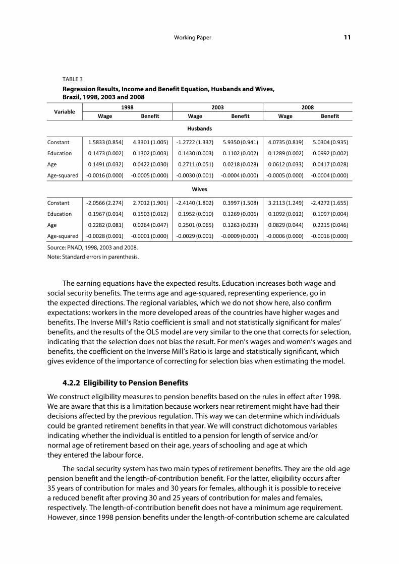
Table 3 presents the results for husbands’ and wives’ human capital equations, for wage and benefits. We use the same set of explanatory variables for both equations. We assume that since wages are dependent on individual characteristics and pension benefits are dependent on wages, this would give the best possible outcome. The selection problem arises because we do not observe workers’ wages and benefits at the same point in time. Therefore, we have an unmeasured variable that affects both the dependent variable and the chances of a person being in the sample (Heckman 1979; Greene 2003).

Working Paper 11

TABLE 3

Regression Results, Income and Benefit Equation, Husbands and Wives, Brazil, 1998, 2003 and 2008

Variable 1998 2003 2008

Wage Benefit Wage Benefit Wage Benefit

Husbands

Constant 1.5833 (0.854) 4.3301 (1.005) ‐1.2722 (1.337) 5.9350 (0.941) 4.0735 (0.819) 5.0304 (0.935)

Education 0.1473 (0.002) 0.1302 (0.003) 0.1430 (0.003) 0.1102 (0.002) 0.1289 (0.002) 0.0992 (0.002)

Age 0.1491 (0.032) 0.0422 (0.030) 0.2711 (0.051) 0.0218 (0.028) 0.0612 (0.033) 0.0417 (0.028)

Age‐squared ‐0.0016 (0.000) ‐0.0005 (0.000) ‐0.0030 (0.001) ‐0.0004 (0.000) ‐0.0005 (0.000) ‐0.0004 (0.000)

Wives

Constant ‐2.0566 (2.274) 2.7012 (1.901) ‐2.4140 (1.802) 0.3997 (1.508) 3.2113 (1.249) ‐2.4272 (1.655)

Education 0.1967 (0.014) 0.1503 (0.012) 0.1952 (0.010) 0.1269 (0.006) 0.1092 (0.012) 0.1097 (0.004)

Age 0.2282 (0.081) 0.0264 (0.047) 0.2501 (0.065) 0.1263 (0.039) 0.0829 (0.044) 0.2215 (0.046)

Age‐squared ‐0.0028 (0.001) ‐0.0001 (0.000) ‐0.0029 (0.001) ‐0.0009 (0.000) ‐0.0006 (0.000) ‐0.0016 (0.000)

Source: PNAD, 1998, 2003 and 2008.

Note: Standard errors in parenthesis.

The earning equations have the expected results. Education increases both wage and social security benefits. The terms age and age-squared, representing experience, go in the expected directions. The regional variables, which we do not show here, also confirm expectations: workers in the more developed areas of the countries have higher wages and benefits. The Inverse Mill’s Ratio coefficient is small and not statistically significant for males’ benefits, and the results of the OLS model are very similar to the one that corrects for selection, indicating that the selection does not bias the result. For men’s wages and women’s wages and benefits, the coefficient on the Inverse Mill’s Ratio is large and statistically significant, which gives evidence of the importance of correcting for selection bias when estimating the model.

4.2.2 Eligibility to Pension Benefits

We construct eligibility measures to pension benefits based on the rules in effect after 1998. We are aware that this is a limitation because workers near retirement might have had their decisions affected by the previous regulation. This way we can determine which individuals could be granted retirement benefits in that year. We will construct dichotomous variables indicating whether the individual is entitled to a pension for length of service and/or normal age of retirement based on their age, years of schooling and age at which they entered the labour force.

The social security system has two main types of retirement benefits. They are the old-age pension benefit and the length-of-contribution benefit. For the latter, eligibility occurs after 35 years of contribution for males and 30 years for females, although it is possible to receive a reduced benefit after proving 30 and 25 years of contribution for males and females, respectively. The length-of-contribution benefit does not have a minimum age requirement. However, since 1998 pension benefits under the length-of-contribution scheme are calculated


taking into account, in addition to the length of contribution, the worker’s age and life expectancy at that age (called Fator Previdenciario). Thus, those who choose to retire earlier receive a smaller benefit than those who stayed longer in the labour force (Queiroz, 2008; Soares, 2010). Workers are eligible for old-age pension benefits at age 65 for males and 60 for females.

The eligibility for length-of-service and old-age retirement benefits are shown in the following equations, where NR is the normal retirement age, ER is the early retirement age and LS is the period in the labour force.

NR = 1 if Agem > = 65 or Agef > = 60 (3)

ER = 1 if Agem < = 65 and LSm > = 35, or Agef < = 60, and LSf > = 30 (4)

The construction of a variable indicating whether an individual is eligible to the old-age pension benefit is straightforward and shown in Equation 3.

The construction of the variable for early retirement eligibility (Equation 4) is a little more complicated, since the survey does not have information on work tenure. First, we considered only those younger than the old-age requirement. Second, we combine the information on the age at which an individual started to work and years of schooling to construct this measure. We add to the age at which a person reported started working the years of obtained education after that age. If the sum is equal to or greater than 35 (30) years, the worker is eligible for length-of-service benefit.

4.2.3 Individual Characteristics

Age is the most important variable explaining retirement. We estimate the models using age in different ways: as a linear variable, quadratic, cubic, as identification variables for age groups, and combinations. By using dummies, we expect to capture peaks on retirement probabilities at certain ages, especially the normal retirement ages regulated by the system.

Education also plays a role in retirement behaviour. Education is highly correlated with income, wealth and the type of job an individual holds. The net effect of education will be the result of income and substitution effects. The first creates more incentives to retire, since more educated workers are more able to afford retirement, while the latter implies higher opportunity costs to leave work. Education is also related to the age at which a worker enters the labour force. We assume that workers with lower levels of education entered the labour force at an earlier age. We also assume that these workers normally work in more physically demanding jobs, which can play a role in the decision of whether to leave the labour force.

Occupation is related to the educational level but also to access to social security benefits. Workers in the formal market have more direct access to social security than workers in the informal sector and self-employed workers. The first are enrolled in the system by their employers, while the second have to decide on their own whether to join the pension system. This variable will give a good indication of the impacts of the pension system on the retirement propensities of workers in Brazil.

Working Paper 13

4.2.4 Familial Incentives

We constructed different measures of family incentives. We expect the labour force status of the one spouse to have an important influence on the retirement decision of the other. We construct this measure in two ways: for the stock regression we simply include a variable indicating whether the spouse is retired; for the flow models we constructed a variable indicating whether or not the spouse retired during that year. We also estimate the couple’s age differences using information on date of birth of each spouse. The hypothesis is that couples with different age differentials would behave differently. More specifically, we postulate that couples closer in age have higher propensity to retire at the same time because they share similar trajectories in the labour market.

We use a variable to control for the existence of dependent children in the household, considering children under the age of 14 years of age as dependents. Our hypothesis is that households with dependent children would stay in the labour force because of higher consumption demands that might not be fulfilled with pension benefits.

The last variable we use is the health status of each spouse. The assumption is that having a spouse with bad health would lead individuals to seek retirement to provide help. The problem of using current health status is reverse causality: health status affects the ability to work, but not being in the labour force might affect one’s health, and employment also affects health (Smith, 1999). In addition to that, the PNAD does not provide information on previous health status or the occurrence of health shocks that might have affected labour force participation. One last problem is unobservable characteristics that influence labour supply decisions and health status at the same time (McGarry, 2004).

5 JOINT RETIREMENT AND LABOUR SUPPLY DECISIONS

5.1 THE IMPACTS OF SPOUSES ON LABOUR FORCE STATUS

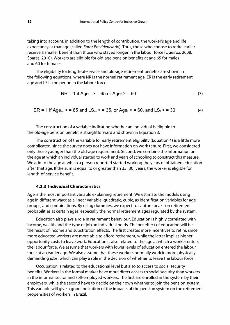
In Table 4 we present the marginal effects of wives’ labour force status on husbands’ retirement, and vice-versa, using a probit model. The results tell a fairly consistent story. In 1998, husbands whose wives were in the labour force (working or seeking jobs) experienced a relative decrease in their retirement probabilities, and women whose spouses were in the labour force experienced a relative increase in their retirement probabilities.

In 2008, however, wives seem not to take into account their husbands’ labour force status in their retirement decisions. Men respond more sensitively and positively to women’s retirement status rather than vice-versa. The positive or null effect of having an active spouse for women’s retirement decisions might be indicating either that since older women’s labour force participation is still relatively low, those in the labour force have more incentives to stay than leave, or maybe that they might need to stay in the labour force to complement household income.

The other variables behave as expected: retirement probability increases with age, more educated workers have higher probability of retirement, having dependent children at home reduces probability of retirement, and poor health status also increases chances of retiring, but in some cases they are not statistically significant.

TABLE 4

The Estimated Effect of Having a Retired Spouse on Retirement Transition, Marginal Effects, Brazil, 1998, 2003 and 2008

Variable 1998 2003 2008

Husbands Wives Husbands Wives Husbands Wives

1: Only Spouse’s status ‐0.0813 (0.0091) ‐0.0144 (0.0122) ‐0.0747 (0.0076) ‐0.0406 (0.0103) ‐0.0814 (0.0067) ‐0.0528 (0.0090) 2: 1 + Age ‐0.0386 (0.0093) 0.0169 (0.0099) ‐0.0296 (0.0074) 0.0064 (0.0073) ‐0.0247 (0.0061) 0.0057 (0.0054) 3: 2 + Education ‐0.0438 (0.0093) 0.0194 (0.0084) ‐0.0325 (0.0074) 0.0053 (0.0068) ‐0.0291 (0.0061) 0.0029 (0.0053) Including all covariates ‐0.0419 (0.0093) 0.0200 (0.0084) ‐0.0315 (0.0074) 0.0054 (0.0068) ‐0.0288 (0.0061) 0.0030 (0.0053)

Source: PNAD, 1998, 2003 and 2008. Note: Standard errors in parenthesis.

TABLE 5

Bivariate Probit, Probability of Retirement Transition, Couples, Brazil, 1998, 2003 and 2008

Variable

1998 2003 2008

Husband’s Outcome

Wife’s Outcome

Husband’s Outcome

Wife’s Outcome

Husband’s Outcome

Wife’s Outcome

Benefit Rep. Rate Husband’s 3.952 (2.6740) 6.980 (3.0578) 1.666 (0.7541) 2.210 (0.8326) ‐15.416 (12.8169) 41.584 (12.8244) Wife’s ‐0.117 (0.0596) 0.092 (0.0631) ‐0.242 (0.1536) 0.812 (0.2016) 5.206 (4.2434) 2.490 (5.9063)

Elegibility Soc. Sec.

Husband Old‐Age ‐0.101 (0.0948) ‐0.107 (0.1179) 0.041 (0.0824) ‐0.214 (0.1009) 0.138 (0.0681) ‐0.035 (0.0838) Husband LS ‐0.134 (0.1505) 0.251 (0.1689) ‐0.188 (0.1257) 0.253 (0.1384) ‐0.350 (0.0847) ‐0.132 (0.0950) Wife Old‐Age ‐0.007 (0.0909) ‐0.004 (0.1069) ‐0.147 (0.0780) 0.319 (0.0923) ‐0.058 (0.0730) 0.039 (0.0855) Wife LS ‐0.175 (0.1144) ‐0.150 (0.1275) 0.045 (0.1010) 0.097 (0.1112) 0.066 (0.1089) 0.062 (0.1115)Age Husband’s 0.075 (0.0111) ‐0.018 (0.0127) 0.081 (0.0087) ‐0.004 (0.0097) 0.080 (0.0195) 0.060 (0.0210) Wife’s 0.005 (0.0102) 0.088 (0.0126) 0.033 (0.0102) 0.069 (0.0128) 0.001 (0.0238) 0.126 (0.0271)

Education Husband’s 0.065 (0.0133) 0.015 (0.0152) 0.049 (0.0109) 0.020 (0.0123) ‐0.035 (0.0497) 0.148 (0.0507) Wife’s 0.006 (0.0077) 0.109 (0.0097) ‐0.004 (0.0084) 0.102 (0.0108) ‐0.014 (0.0126) 0.052 (0.0158)Health Status, Poor=1 Husband’s 0.129 (0.0527) ‐0.006 (0.0635) ‐0.067 (0.0483) 0.029 (0.0583) ‐0.088 (0.0444) ‐0.042 (0.0508) Wife’s ‐0.066 (0.0529) 0.092 (0.0636) ‐0.035 (0.0487) 0.020 (0.0578) ‐0.043 (0.0449) 0.041 (0.0513)Dep. Children, No=1 0.221 (0.0602) 0.102 (0.0733) 0.087 (0.0609) ‐0.004 (0.0753) 0.076 (0.0689) 0.169 (0.0926)

Labour Status, Formal=1 ‐0.157 (0.0513) ‐0.077 (0.0638) ‐0.226 (0.0477) ‐0.134 (0.0554) ‐0.236 (0.0435) ‐0.145 (0.0531)Constant ‐9.460 (2.6599) ‐13.481 (3.1002) ‐9.010 (0.9780) ‐9.972 (1.1395) 6.036 (14.4816) ‐56.253 (14.7978)

rho 0.2746 (0.0355) 0.3280 (0.0316) 0.3130 (0.0304)

Source: PNAD, 1998, 2003 and 2008. Note: Standard errors in parenthesis.

Working Paper 15

5.2 THE DETERMINANTS OF RETIREMENT TRANSITION

We now turn to the analysis of the joint retirement decision model using the bivariate probit model. Table 5 shows the results for all three years for both husbands and wives. The dependent variable is the change in the individual’s labour force status in the week of reference compared to the status in the year of reference (flow of retirees). Explanatory variables are: benefit replacement rate, eligibility to pension benefits, age, education, health status, presence of dependent children in the household and status in the labour market before retirement (formal or informal).

Our analysis is limited by the small number of individuals who reported a transition in that particular year (around 18 per cent of men and 10 per cent of women for all samples). Nevertheless, we observe some interesting patterns worth comparing with the probability of being retired in a particular year.

First, we turn our attention to the correlation between the two outcome equations to test the joint retirement hypothesis. The estimate of rho is 0.324 in 2008 and 0.282 in 1998, with marginal significance of 0.0337 and 0.0384, respectively, providing statistical significance in favour of the joint retirement hypothesis. In light of earlier discussion, the results indicate that couples tend to retire at the same time.

The most striking difference between 1998 and 2008 is the impact of benefit replacement rate on retirement behaviour. The impact of husbands’ replacement rate on wives’ retirement is positive for both years; the magnitude of the coefficient increased six-fold. We also observed that in 1998 higher replacement rate for wives reduced the probability of their husband’s retirement, and this effect disappeared in 2008.

Age affects retirement decisions in several ways. The two most important ones are the eligibility for pension benefits and increase in utility for leisure. We find that a person’s age increases the propensity of retirement, as older individuals have a higher chance of being retired. Spouse’s age also affects retirement behaviour but in different ways. Spouse’s age has opposite impacts: being married to an older man increases the chance of wives being retired by 0.0602 in 2008, although the effect is not observed in 1998. However, being married to older women seems not to have any impact on male retirement in either 1998 or 2008.

For males, being eligible for an old-age pension benefit (65 years old or more) increases by 0.138 the chances of transitioning to retirement. The impact for females is also positive but not statistically significant. For males, being eligible for early retirement reduces by 0.35 the probability of retirement. The main reason for that might be the impact of the new formula to calculate pension benefits that takes into account an individual’s age at retirement, life expectancy at that age and period of contribution. In 1998 we do not find significant effects of being eligible to pension benefits (early retirement or old-age). We believe this is the result of the changes in retirement rules in 1998, since people who were closer to retirement decided to leave the labour force before the changes took place. Thus, those who remained in the labour force, now under the new rules, had to work longer to receive their benefit.

For females in 2008 not only does their own educational status have a strong and positive effect on their retirement transition (0.148), but so does their husband’s educational status (0.0524). The impact on the husband’s retirement is negative but not statistically significant. In this model, education is indicating the net effect of income and substitution effects.


We are assuming that more educated workers command a higher wage and higher pension benefits, which are positively correlated to larger social security wealth. A positive value indicates that income effect is higher, so more educated workers have more ability to afford retirement and do retire earlier. In case of females, it is possible that more educated females were able to have a steadier working career, meaning that they were able to contribute to the public pension system more regularly, thus being able to retire at earlier ages than their less educated counterparts.

In 1998 we observed that being in poor health increased the chances of retirement for husbands. For wives, the impact is not statistically significant. We also do not find any spillover effect of one spouse’s health on the other’s retirement behaviour. Spouse’s health status affects the decision to retire during the year in a counterintuitive way in 2008. For husbands, being in poor health and having a wife in poor health reduces the probability of retirement. For wives, being in poor health increases her chances of retiring, but having a husband in poor health reduces her chances of retirement. Our hypothesis was that wives’ health would have a negative impact on husbands’ retirement because of financial needs, for instance, to afford possible extra health care costs. However, we believe that more analysis of this issue is necessary.

Surprisingly, self-employed and informal workers are more likely to be retired than individuals employed in the formal sector who, theoretically, have more and easier access to social security benefits. Lastly, for both husbands and wives, having dependent children at home increases the chances of retirement in 2008.3

5.3 THE DETERMINANTS OF RETIREMENT TRANSITION: POOLED DATA ANALYSIS

We now estimated the model using pooled data for the three PNADS (1998, 2003 and 2008). The main advantage is that we can increase sample size and perform more analysis on the data, and we are also interested in capturing the period effects on the joint retirement behaviour of couples in Brazil. Table 6 shows the results for the pooled data for husbands and wives. As in the previous model, the dependent variable represents the change in status in the labour force (flow of retirees), and explanatory variables are: benefit replacement rate, eligibility to pension benefits, age, education, health status, presence of dependent children in the household and status in the labour market before retirement (formal or informal).

First, we turn our attention to the correlation between the two outcome equations to test the joint retirement hypothesis. The estimated value of rho is positive (0.3171) and statistically significant (0.0185), indicating that husbands and wives tend to leave the labour force around the same time (as discussed before). In addition, the results indicate that models should be estimated in a bivariate probit model instead of two separate regression models for husbands and wives.

We find that benefit replacement rate has a strong effect on retirement transitions for both husbands and wives. The effect of husbands’ replacement rate on wives’ retirement decision is three times larger than on husbands’ own decisions. The result indicates that income effect plays an important role for older cohorts of women in the Brazilian labour market. We also observe that wives’ replacement rate have a negative impact on husbands’ retirement decisions. For husbands, being in poor health and having a wife in poor health reduces the probability of retirement. For wives, being in poor health increases her chances of retiring,

Working Paper 17

but having a husband in poor health reduces her chances of retirement. We find that an individual’s age increases the propensity of being out of the labour force, as older individuals have a higher chance of being retired. We observed that more educated workers have higher propensity to retire, and being married to a more educated husband also increases wives’ retirement propensity. Finally, we observe for wives that having a husband eligible to retire increases her chances of leaving the labour force during the period of analysis.

TABLE 6

Bivariate probit, Probability of Retirement Transition, Couples, Brazil, 1998, 2003 and 2008 (pooled data)

Variable Husband’s Outcome Wife’s Outcome

Benefit Rep. Rate

Husband’s 2.818 (1.5379) 6.016 (1.7530)

Wife’s ‐0.706 (0.2522) 1.812 (0.2876)

Elegibility Soc. Sec.

Husband Old‐Age 0.068 (0.0478) ‐0.133 (0.0594)

Husband LS ‐0.267 (0.0728) 0.137 (0.0806)

Wife Old‐Age ‐0.076 (0.0454) 0.167 (0.0541)

Wife LS ‐0.017 (0.0598) 0.092 (0.0654)

Age

Husband’s 0.082 (0.0066) ‐0.014 (0.0074)

Wife’s 0.032 (0.0071) 0.070 (0.0084)

Education

Husband’s 0.049 (0.0095) 0.023 (0.0108)

Wife’s ‐0.009 (0.0064) 0.115 (0.0078)

Health Status, Poor=1

Husband’s ‐0.024 (0.0275) ‐0.010 (0.0329)

Wife’s ‐0.038 (0.0277) 0.052 (0.0329)

Dep. Children, No=1 0.134 (0.0364) 0.084 (0.0453)

Labour Status, Formal=1 ‐0.212 (0.0271) ‐0.135 (0.0327)

Year 2003 ‐0.203 (0.0312) ‐0.168 (0.0373)

Year 2008 ‐0.392 (0.0308) ‐0.334 (0.0367)

Constant ‐9.138 (1.4684) ‐14.041 (1.7054)

rho 0.3171 (0.0185)

Source: PNAD, 1998, 2003 and 2008.

Note: Standard errors in parenthesis.

More interesting, we observed a clear period effect on retirement transition over time for both husbands and wives. The probability of retiring was greater in 1998 than in 2003 and 2008. We argue that this is mainly the impact of recent changes in social security rules that create incentives to stay in the labour force. It is also possible that younger generations


of workers are better educated and have better job conditions than previous ones, thus remaining longer in the labour force. However, it is important to stress that retirement ages in Brazil were quite low. According to the Brazilian Ministry of Social Security (MPAS) median retirement age in 2000 was estimated around 63 for males, and retirement under the length-of-contribution scheme was estimated to be around 48 years old in 1998, increasing to about 54 in 2006.

6 DISCUSSION AND FUTURE WORK

We observe that social security regulations in Brazil, as in many other countries, provide incentives for the working population to postpone retirement until the age at which benefits are available but do not create incentives to stay in the labour force after that age. Labour force participation rates for older men fell significantly between 1950 and 2000. During this time, the Brazilian pension system expanded, absorbing a larger group of the population and helping to accelerate the trends toward early retirement.

The main interest of this paper was, however, to understand how the spouse’s retirement behaviour is influenced by their own characteristics and by interdependent variables (spillover effects). We find that husbands and wives respond similarly to their own personal characteristics and variables, in the direction discussed in the literature. We also find strong evidence of joint retirement decisions, since having a spouse out of the labour force increases the probability of one’s own decision of being out of the labour market.

The results presented in this paper should be interpreted with caution. The use of cross-sectional data for the study of life-cycle behaviours is very complicated and poses several problems. However, in the absence of longitudinal data in developing countries, the existence of large and high-quality cross-sectional household surveys may shed some light on this problem.

The system also plays a perverse role by creating more incentives to early retirement for workers with higher income and better socioeconomic status. The system, which was created to transfer income from wealthy people to poor people, is operating in the opposite way. At this point, we are working on setting up the data to perform an analysis following a pseudo-cohort, and a simulation model to address how changes in the rules and regulations of the system could affect couples’ retirement behaviour (since there are important changes in the pension system in the period of analysis, we are working on using those changes as possible shocks to better investigate couples’ behaviour in the Brazilian labour market).

It is also important to investigate the impact of the labour market and economic conditions in the period and how they could affect labour supply behaviour. Unemployment rates fell from about 12 per cent in 1998 to around 7 per cent in 2008. Also, there is an important change in the composition of the labour force, as more women and more educated workers are reaching older age or are getting closer to retirement ages in 2008 than in 1998.

Working Paper 19

REFERENCES

Aguila, E. (2012) Male Labor Force Participation and Social Security in Mexico. Santa Monica, CA: RAND Corporation. <http://www.rand.org/pubs/working_papers/WR910>.

Ansiliero, G. and Paiva, L.H. (2008). ‘The recent evolution of social security coverage in Brazil’, International Social Security Review, Vol. 61, No. 3.

Blau, D.M. (1998). ‘Labor Force Dynamics of Older Married Couples’, Journal of Labor Economics, 16:595–629.

Bloom, D. and McKinnon, R. (2010). ‘Social security and the challenge of demographic change’, International Social Security Review, Vol. 63, No. 3–4.

Bongaarts, J. (2004). ‘Population Aging and the Rising Cost of Public Pensions’, Population and Development Review, 30:1–23.

Bowen, W.G. and Finegan, T.A. (1969). The Economics of Labor Force Participation. Princeton, NJ, Princeton University Press.

Carvalho-Filho, I. (2008). ‘Old-Age Benefits and Retirement Decisions of Rural Elderly in Brazil’, Journal of Development Economics, 80:129–146.

Coile, C. (2004). ‘Retirement Incentives and Couples’ Retirement Decisions’, Topics in Economic Analysis & Policy, Vol. 4: No. 1, Article 17.

Costa, D.L. (1998). The evolution of retirement: an American economic history: 1880–1990. Chicago, IL, University of Chicago Press.

Giambiagi, F. and Alem, A.C.D. (1997). ‘A Despesa Previdenciaria no Brasil: evolucao, diagnostico e perspectivas’, Texto para Discussao, No. 374. Brasília, IPEA.

Giambiagi, F. and L. B. d. Castro (2003). ‘Previdência Social: Diagnósticos e Propostas de Reforma’, Revista do BNDES, 10: 265-292.

Giatti, L. and Barreto, S. M. (2003) Saúde, trabalho e envelhecimento no Brasil. Caderno de Saúde Pública, Rio de Janeiro, v. 19, n. 3.

Greene, W. (2003). Econometric Analysis, 5th edition. Upper Saddle River, NJ, Prentice Hall.

Gruber, J. and Wise, D. (eds.) (1999). Social Security and Retirement Around the World. Chicago, IL, University of Chicago Press.

Gruber, J. and Wise, D. (eds.) (2004). Social Security and Retirement Around the World: micro-estimation. Chicago, IL, University of Chicago Press.

Gustman, A. and Steinmeier, T. (2000). ‘Retirement in Dual-Career Families: a structural model’, Journal of Labor Economics, 18:503–545.

Heckman, J. (1979). ‘Sample Selection Bias as a Specification Error’, Econometrica, 47:153–61.

Henretta, J.C. and O’Rand, A.M. (1983). ‘Joint Retirement in the Dual Worker Family’, Social Forces, 62:504–520.

Hurd, M. (1990). ‘The Joint Retirement Decision of Husbands and Wives’ in D. Wise (ed.), Issues in the Economics of Aging, 231–258. Chicago, IL, University of Chicago Press.


Lazear, E. (1986). ‘Retirement from the Labor Force’ in O. Ashenfelter and R. Layard (eds), Handbook of Labor Economics, Vol. 1, 5: 305–355. Amsterdam, Elsevier Science Publishers.

Legrand, T. (1995). ‘The Determinants of Men’s Retirement Behavior in Brazil’, The Journal of Development Studies, 31:673–701.

Lumsdaine, R. and Mitchell, O. (1999). ‘New Developments in the Economic Analysis of Retirement’ in O. Ashenfelter and R. Layard (eds), Handbook of Labor Economics, Vol. 3, 49: 3261–3307. Amsterdam, Elsevier Science Publishers.

Maestas, N. (2001). ‘Labor, Love and Leisure: complementarity and the timing of retirement by working couples’, Working Paper. Berkeley, CA, University of Berkeley Department of Economics.

Mason, A., Lee, R. and Lee, S. (2010). ‘Population Dynamics: social security, market and the families’, International Social Security Review, Vol. 63, No. 3–4.

McGarry, K. (2004). ‘Health and Retirement: do changes in health affect retirement expectantions?’, The Journal of Human Resources, 39.

Pozzenbon, S. and Mitchell, O. (1989). ‘Married Women’s Retirement Behavior’, Journal of Population Economics, 2:39–53.

Queiroz, B. (2008). ‘Retirement Incentives: Pension Wealth, Accrual and Implicit Tax’, Well-Being and Social Policy, Vol. 4.

Queiroz, B. (2007). ‘The Determinants of Males’ Retirement in Urban Brazil’, Nova Economia, Vol. 17(1).

Queiroz, B. (2006). ‘Social Security and Couple’s Joint Retirement Decisions in Brazil’. Paper presented at the Annual Meeting of the Population Association of America, Los Angeles, 2006.

Reimers, C. and Honig, M. (1996). ‘Responses to Social Security by Men and Women: myopic and far-sighted behavior’, The Journal of Human Resources, 31:359–382.

Soares, R. (2010). ‘Aging, Retirement and Labor Supply in Brazil’. Unpublished manuscript presented at the World Bank seminar ‘Aging in Brazil’, Brasília, DF.

Wise, D. (2010). ‘Facilitating Longer Working Lives: International Evidence on Why and How’, Demography, 47, Supplement S131–49.

Wise, D. (2004). ‘Social Security Provisions and the Labor Force Participation of Older Workers’, Population and Development Review, 30, Supplement S176–205.

Zweimuller, J., Winter-Ebmer, R. and Falkinger, J. (1996). ‘Retirement of Spouses and Social Security Reform’, European Economic Review, 40:449–472.

NOTES

1. The age selection is in accordance with the retired population age structure observed in the Brazilian Social Security Administration records.

2. We use two measures of education: years of schooling and educational group (less than four years, between five and eight years, between nine and 11, and more than 12). We find that 68 per cent of the couples in 1998 are in the same educational group. The racial composition of couples shows similar signs: 80 per cent of couples in 1998 were formed by partners of the same race. These findings suggest positive assortative mating which can help explain certain patterns of retirement (Becker, 1993).However, it seems that this behaviour is changing over time, since in 2003 the percentage of couples in the same educational and racial group fell to 57 per cent and 68 per cent, respectively.

3. We check the robustness of these results regarding the endogeneity of some variables included in the model. One alternative would be to obtain an instrumental variable. For example, presence of dependent children is endogenous to the decision to work (for women), and the above mentioned problem of dual causality of health. I did not find any valid instrument for dependent children given my theoretical model and the structure of the data. The alternative is to re-estimate the previous models with different specifications and check the significance of the correlation coefficients. We estimate the model for retiring in the past year with six different specifications (available upon request). The results indicate that the correlation term is robust to the model specification and that couples tend to jointly decide whether to retire or not.

International

Centre for Inclusive Growth

International Policy Centre for Inclusive Growth (IPC - IG)Poverty Practice, Bureau for Development Policy, UNDPEsplanada dos Ministérios, Bloco O, 7º andar70052-900 Brasilia, DF - BrazilTelephone: +55 61 2105 5000

E-mail: [email protected] URL: www.ipc-undp.org

COUPLE’S BEHAVIOUR IN THE BRAZILIAN LABOUR MARKET … · COUPLE’S BEHAVIOUR IN THE BRAZILIAN...

Documents

Transcript of COUPLE’S BEHAVIOUR IN THE BRAZILIAN LABOUR MARKET … · COUPLE’S BEHAVIOUR IN THE BRAZILIAN...