Coupled electromechanical model of the heart: Parallel finite element formulation

INTERNATIONAL JOURNAL FOR NUMERICAL METHODS IN BIOMEDICAL ENGINEERING

Published online in Wiley Online Library (wileyonlinelibrary.com). DOI: 10.1002/cnm.1494

Coupled electromechanical model of the heart: Parallel finiteelement formulation

Pierre Lafortune 1, Ruth Arís 1, Mariano Vázquez 1,*,† and Guillaume Houzeaux 1

1BSC-CNS, Barcelona Supercomputing Center, Barcelona, Spain2IIIA-CSIC, Barcelona, Spain

SUMMARY

In this paper, a highly parallel coupled electromechanical model of the heart is presented and assessed.The parallel-coupled model is thoroughly discussed, with scalability proven up to hundreds of cores. Thiswork focuses on the mechanical part, including the constitutive model (proposing some modifications topre-existent models), the numerical scheme and the coupling strategy. The model is next assessed throughtwo examples. First, the simulation of a small piece of cardiac tissue is used to introduce the main features ofthe coupled model and calibrate its parameters against experimental evidence. Then, a more realistic prob-lem is solved using those parameters, with a mesh of the Oxford ventricular rabbit model. The results ofboth examples demonstrate the capability of the model to run efficiently in hundreds of processors and to

Received 24 June 2011; Revised 25 November 2011; Accepted 30 November 2011

KEY WORDS: cardiac mechanics; electrophysiology; parallelization; finite element methods

1. INTRODUCTION

Computational mechanics plays an important role in many engineering fields, and cardiac mechan-ics is no exception. Nowadays, some models allow realistic simulations of the heart beat, and couldbe used to study different pathologies or to understand better the physiological mechanisms reg-ulating the contraction of the heart [1, 2]. Cardiac mechanics simulations represent a challenge interms of numerical algorithms, programming techniques and computational resources. If today’smodels can take several weeks on single core computers with coarse meshes [3], the use of parallelresources will be essential for tomorrow’s models.

Electromechanical finite element models developed during the last decades improved quicklyin terms of precision and the way they represent the geometry of the heart. However, very fewmodels are prepared to run on large supercomputers. To cite some of them, models developed bySainte-Marie et al. [4], Stevens et al. [5], Göktepe et al. [6], Kerckhoffs et al. [7], Nobile et al. [8]and Gurev et al. [9] have been used successfully to study different aspects of cardiac functions, butare made of relatively small meshes. This lack of resolution is an obstacle when trying to reproducethe complex fibers distribution. Note, on the other hand, that recent work of Hosoi et al. [10] andReumann et al. [11] show very promising results using large meshes and running in parallel onthousands of cores. This paper is an effort in this direction.

In previous work, we have introduced the electrophysiology model [12] and the parallel environ-ment [13] that we use in our framework. This paper addresses the computational mechanics sideof the problem, introducing a highly parallel model capable of running in thousands of processors,

*Correspondence to: Mariano Vázquez, Barcelona Supercomputing Center, Campus Nord UPC, Barcelona, Spain.†E-mail: [email protected]

Int. J. Numer. Meth. Biomed. Engng. (2012)

reproduce some basic characteristic of cardiac deformation. Copyright © 2012 John Wiley & Sons, Ltd.

Copyright © 2012 John Wiley & Sons, Ltd.

P. LAFORTUNE ET AL.

which allows to perform cardiac simulations on realistic conditions, using meshes of millions ofelements with turnaround times of hours.

The computational model is implemented in Alya System, a high performance computationalmechanics code developed in Barcelona Supercomputing Center BSC-CNS. It is a flexible platformfor running in parallel coupled problems using non-structured meshes. The finite element space dis-cretization and the parallelization based on automatic domain decomposition for distributed memoryfacilities are the main features of this strategy. The automatic domain partition is carried out usingthe widely known open source software METIS. Based in a master–slave strategy, one core is usedto partition the problem and send each subdomain mesh to each of the other cores taking part ofthe run. METIS partitions the original mesh by minimizing communication surface between subdo-mains and maximizing load balance. Communication is carried out using message passing interface(MPI). Parallelization is carried out transparently, so, if properly coded, each of the coupled prob-lems retains the scalability properties: the fact that all the coupled problems are solved onto the samemesh avoids interpolation, mesh imbalance, and so on. For a thorough description, refer to [13, 14].

Fully implicit and explicit schemes are implemented. The resulting code is able to run using ele-ments of different space order (P1, P2,. . . , Q1, Q2,. . . ) and higher order time schemes, in 2D and3D domains of a non-homogeneous anisotropic excitable media.

This paper is divided as follows. First, the electrophysiological model is briefly resumed. Then,the mechanical model used, including the constitutive law, is described in detail. This descriptionincludes numerical tests to validate the material law. The description of the coupling model follows.Finally, results of the contraction of a simple geometry and a complete heart model are presentedand compared qualitatively with general physiological motions.

The novelties of this work include: (1) proving the efficiency of a highly parallel-coupled elec-tromechanical model of the heart up to 500 cores, using a realistic geometry; (2) the use of aconstitutive law that is based on a general and flexible framework and that reflects better the behav-ior in compression of the myocardium, and the characterization of this law; and (3) the study andcharacterization of the damping properties of the heart.

2. PHYSIOLOGICAL MODELS

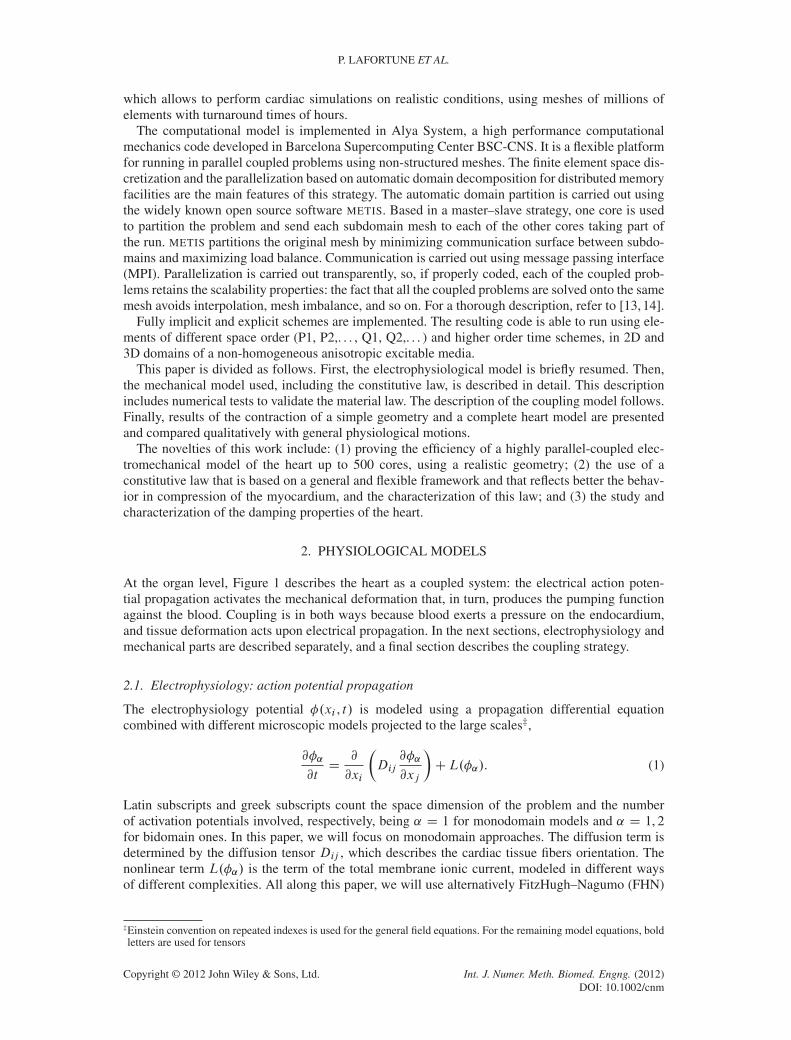
At the organ level, Figure 1 describes the heart as a coupled system: the electrical action poten-tial propagation activates the mechanical deformation that, in turn, produces the pumping functionagainst the blood. Coupling is in both ways because blood exerts a pressure on the endocardium,and tissue deformation acts upon electrical propagation. In the next sections, electrophysiology andmechanical parts are described separately, and a final section describes the coupling strategy.

2.1. Electrophysiology: action potential propagation

The electrophysiology potential �.xi , t / is modeled using a propagation differential equationcombined with different microscopic models projected to the large scales‡,

@�˛

@tD

@

@xi

�Dij

@�˛

@xj

�CL.�˛/. (1)

Latin subscripts and greek subscripts count the space dimension of the problem and the numberof activation potentials involved, respectively, being ˛ D 1 for monodomain models and ˛ D 1, 2for bidomain ones. In this paper, we will focus on monodomain approaches. The diffusion term isdetermined by the diffusion tensor Dij , which describes the cardiac tissue fibers orientation. Thenonlinear term L.�˛/ is the term of the total membrane ionic current, modeled in different waysof different complexities. All along this paper, we will use alternatively FitzHugh–Nagumo (FHN)

‡Einstein convention on repeated indexes is used for the general field equations. For the remaining model equations, boldletters are used for tensors

DOI: 10.1002/cnmCopyright © 2012 John Wiley & Sons, Ltd. Int. J. Numer. Meth. Biomed. Engng. (2012)

COUPLED PARALLEL ELECTROMECHANICAL MODEL OF THE HEART

Figure 1. The heart as a physical system.

[15] or Fenton–Karma (FK) [16] models. For a thorough discussion, see [12]. The weak form ofEquation (1) is: find � 2 V such that 8 2W; the following equation verifies:Z

�

@�

@tdV D

Z@�

Dij

Cm Sv

@�

@xjnjdS �

Z�

Dij

Cm Sv

@

@xi

@�

@xjdV C

Z�

Iion dV (2)

where Cm and Sv are some model constants and Iion is the total membrane ionic current.

2.2. Mechanical deformation: the cardiac muscle

2.2.1. Governing equations. Let �o be a fixed reference configuration of a body and � thedeformed one. The position vector of a particle of that body is expressed by XI in the first con-figuration and by xi in the second one. Note that capital letters and subscripts are used for scalarsor tensors defined in the reference configuration, and lowercase letters and subscripts, when definedin the deformed configuration. The relation between both measures is given by the deformationgradient tensor:

FiJ D@xi

@XJD ıiJ C

@ui

@XJ(3)

where the displacement is ui D xi � XI . The local form of the linear momentum balance, to besolved using a total Lagrangian finite element formulation in the configuration �o, is written asfollows:

�o@2ui

@t2D@PiJ

@XJC �oBi , (4)

which in its weak form isZ�o

ˆ�o@2ui

@t2D�

Z�o

@ˆ

@xJPiJ C

Z@�o

NJPiJˆC

Z�o

ˆ�oBi (5)

where ˆ is a test function, �o is the initial density of the body, NJ is the exterior normal of �oon @�o, Bi is the body force and PiJ is the first Piola–Kirchhoff stress tensor. After discretization,Equation (5) can be expressed in matrix form. Space is discretized using the finite element method(FEM), using the usual compact support space. Time is discretized with finite differences method(FD) using a �-generalized scheme. Alya includes explicit and implicit formulations, but we willfocus in the explicit ones in this paper.

Time–space discretization of this kind of equations leads to a matrix equation of the form

M RuCC .u/ PuCK .u/uDR (6)

whereR is the residual forces vector,M is the mass matrix andK .u/ is the stiffness matrix, whichtypically depends on the unknown. The second term, proportional to the speed, is the Rayleighdamping, where C .u/ is the damping matrix. This matrix is added to damp high frequencies andavoid unphysical oscillations. Usually, its is written as C .u/ D ˛M C ˇK .u/, where parameters˛ and ˇ are computed depending on the frequency range to be damped [17]. After some numericalexperiments, we have observed that the best choice is to take ˇ D 0 and ˛ D c !, where c is aconstant between 2 and 10. The frequency ! is computed by running a problem without damping,


P. LAFORTUNE ET AL.

plotting the displacement for one point in the domain and analyzing its time series. It is worth toremark that when ˇ D 0, the matrix damping becomes independent of the unknown, which certainlysimplifies its computation.

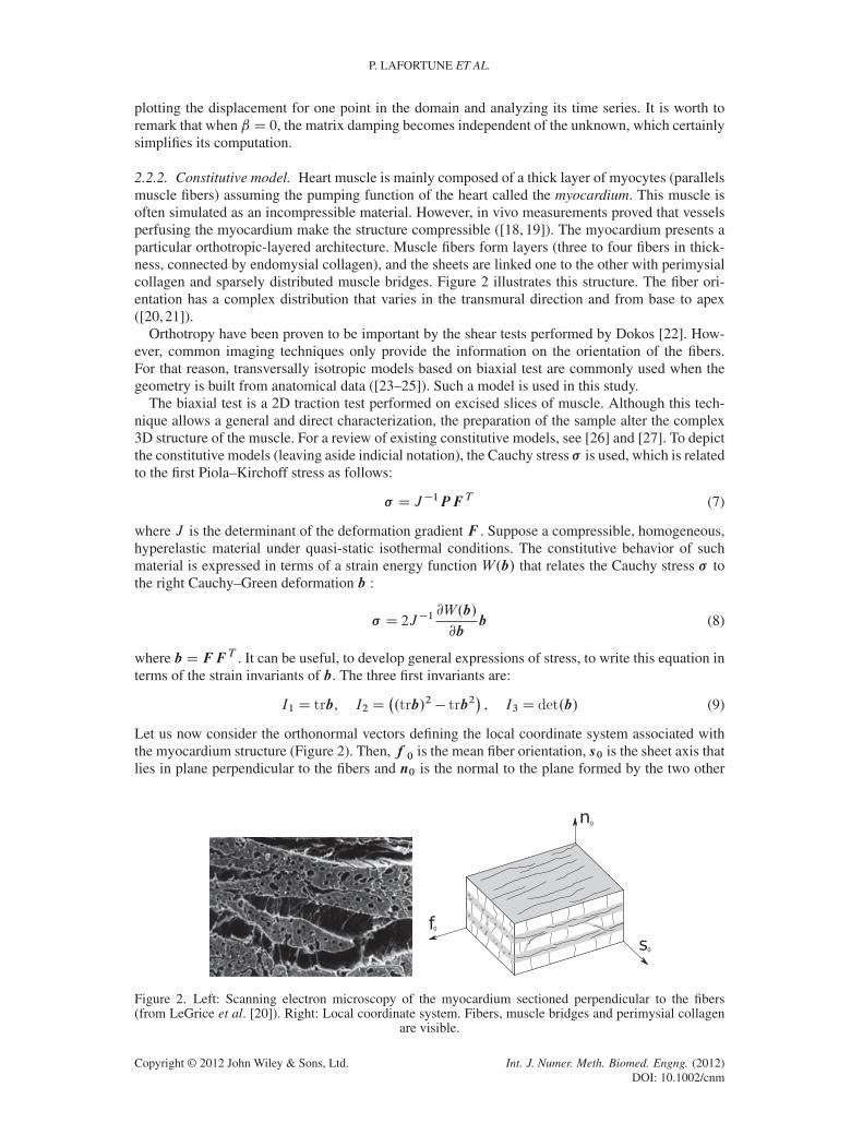
2.2.2. Constitutive model. Heart muscle is mainly composed of a thick layer of myocytes (parallelsmuscle fibers) assuming the pumping function of the heart called the myocardium. This muscle isoften simulated as an incompressible material. However, in vivo measurements proved that vesselsperfusing the myocardium make the structure compressible ([18, 19]). The myocardium presents aparticular orthotropic-layered architecture. Muscle fibers form layers (three to four fibers in thick-ness, connected by endomysial collagen), and the sheets are linked one to the other with perimysialcollagen and sparsely distributed muscle bridges. Figure 2 illustrates this structure. The fiber ori-entation has a complex distribution that varies in the transmural direction and from base to apex([20, 21]).

Orthotropy have been proven to be important by the shear tests performed by Dokos [22]. How-ever, common imaging techniques only provide the information on the orientation of the fibers.For that reason, transversally isotropic models based on biaxial test are commonly used when thegeometry is built from anatomical data ([23–25]). Such a model is used in this study.

The biaxial test is a 2D traction test performed on excised slices of muscle. Although this tech-nique allows a general and direct characterization, the preparation of the sample alter the complex3D structure of the muscle. For a review of existing constitutive models, see [26] and [27]. To depictthe constitutive models (leaving aside indicial notation), the Cauchy stress � is used, which is relatedto the first Piola–Kirchoff stress as follows:

� D J�1PF T (7)

where J is the determinant of the deformation gradient F . Suppose a compressible, homogeneous,hyperelastic material under quasi-static isothermal conditions. The constitutive behavior of suchmaterial is expressed in terms of a strain energy function W.b/ that relates the Cauchy stress � tothe right Cauchy–Green deformation b :

� D 2J�[email protected]/

@bb (8)

where bD FF T . It can be useful, to develop general expressions of stress, to write this equation interms of the strain invariants of b. The three first invariants are:

I1 D trb, I2 D�.trb/2 � trb2

�, I3 D det.b/ (9)

Let us now consider the orthonormal vectors defining the local coordinate system associated withthe myocardium structure (Figure 2). Then, f 0 is the mean fiber orientation, s0 is the sheet axis thatlies in plane perpendicular to the fibers and n0 is the normal to the plane formed by the two other

Figure 2. Left: Scanning electron microscopy of the myocardium sectioned perpendicular to the fibers(from LeGrice et al. [20]). Right: Local coordinate system. Fibers, muscle bridges and perimysial collagen

are visible.



vectors. If such a material is modelized as a transversally isotropic one, the fourth strain invariantwill be also needed:

I4 D f0bf0 (10)

The invariants are of particular interest when developing constitutive laws because they remainunchanged when expressed in a different basis. Using the chain rule,

@W.b/

@bDXa

@W

@Ia

@Ia

@b(11)

and the definitions of the strain invariant derivatives, Equation (8) is reformulated as follows:

� D 2J�1W1bC 2J�1W2

�I1b� b

2�C 2JW3I C 2J

�1W4 Nf ˝ Nf (12)

where the notation Wi D @W=@Ia is used and Nf D Ff 0. This notation is used to underline thefact that Nf is not a unitary vector. See [28] for a more detailed derivation of those equations. Thelast equation is a general framework valid for any hyperelastic material having one preferred ori-entation. The form of W is to be determined. Holzapfel and Ogden [29] suggested a form of Wbased on physiological considerations. The invariant I1 represents the non-collagenous material,whereas invariant I4 represents the stiffness of the muscle fibers. These authors proposed a morecomplete orthotropic law. In this paper, a reduced transversally isotropic version is presented. Wethen propose an energy function given by

W Da

2beb.I1�3/ �

a

2.I1 � 3/C

af

2bf

nebf .I4�1/

2

� 1oCK

2.J � 1/2 (13)

This equation is slightly different from that of [29]. First, a volumetric energy term function of Jhave been added to make the material compressible. Then, the term �a

2.I1 � 3/ is necessary to

respect the initial conditions (zero energy and stress in the reference configuration). This modifica-tion is required owing to the fact that the original incompressible law has a term �pI that makesthe energy equal to zero when no deformations are present. Finally, introducing the expression ofthe derivatives of the energy in the general stress equation gives the following:

J� D�aeb.I1�3/ � a

�bC 2af .I4 � 1/e

bf .I4�1/2 Nf ˝ Nf CK.J � 1/I (14)

where a, b, af , bf are parameters to be determined experimentally. The value ofK is related to thecompressibility and a value of 100 kPa is used as a starting point [30].

To find the constants and validate the constitutive model, the biaxial test conducted by Yin andcoworkers [31] is reproduced. A thin square sheet of tissue of about 4 � 4 � 0.15 cm3 is extractedfrom the myocardium. The traction axis are aligned with the fiber (f ) and cross-fiber (or sheet)direction (s). The third direction perpendicular to this plane is called the normal direction (n)(see Figure 2). First, the stress equation (14) is solved numerically using the gradient deforma-tion tensor F D diag

��f �s�n

. The subscripts refer to the directions described earlier, and � is the

stretch in the indicated direction. �f and �s are given (supposing a displacement-controlled test)and �n is found solving the following:

�n D�ae.b.I1�3// � a

��2nCK.J � 1/D 0 (15)

because no constraint is applied in this direction. This equation is solved numerically using thebisection method. The stress in the two other directions are then calculated with

�f D�ae.b.I1�3// � a

��2f C 2af .I4 � 1/e

bf .I4�1/2

�2f CK.J � 1/ (16)

�s D�ae.b.I1�3// � a

��2s CK.J � 1/ (17)

DOI: 10.1002/cnmInt. J. Numer. Meth. Biomed. Engng. (2012)Copyright © 2012 John Wiley & Sons, Ltd.

P. LAFORTUNE ET AL.

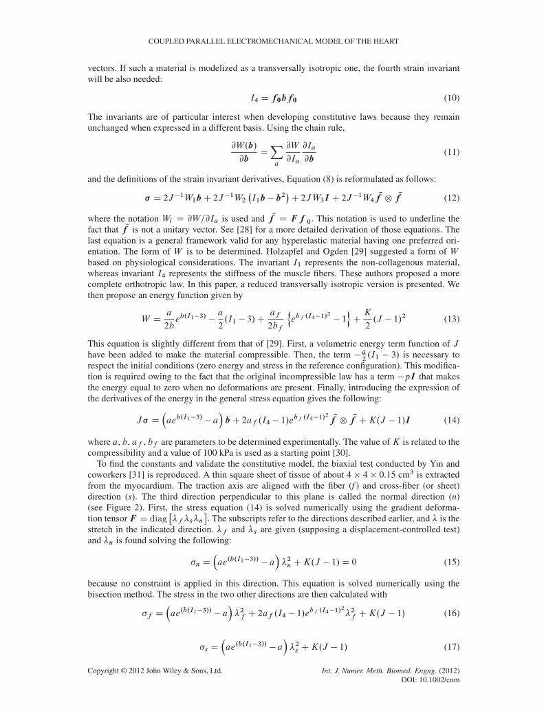
where the constant values are a D 4.3 kPa, b D 9.7, af D 1.69 kPa, bf D 15.78. In addition tothe numerical solution used to find the parameters, the model is tested reproducing the biaxial testswith a simple FE model containing 50 linear hexahedral elements. The results of those tests, alongwith experimental data, are shown on Figure 3.

During systole, the fibers contract and the material is in compression. This behavior is hardlynever studied, neither numerically nor experimentally. It is still a challenge to characterize a materialin compression, even more if it is a complex biological structure. This difficulty probably explainsthe lack of data and numerical test present in the literature. Nevertheless, we can have a generalidea using the solution of a uniaxial traction test. The deformation gradient tensor is, in this case,simplified to F D diag

��f �s�s

, where f is the fiber direction aligned with the traction, and s

the two other directions forming a perpendicular plan to f . Once again, we suppose here that �fis the displacement of the traction machine, and we find �s by solving the stress equation in the sdirections:

�s D�ae.b.I1�3// � a

�.�2s /CK.J � 1/D 0 (18)

Then, the stress in the f direction can be computed as follows:

�f D�ae.b.I1�3// � a

� ��2f

�C 2af .I4 � 1/e

bf .I4�1/2

�2f CK.J � 1/ (19)

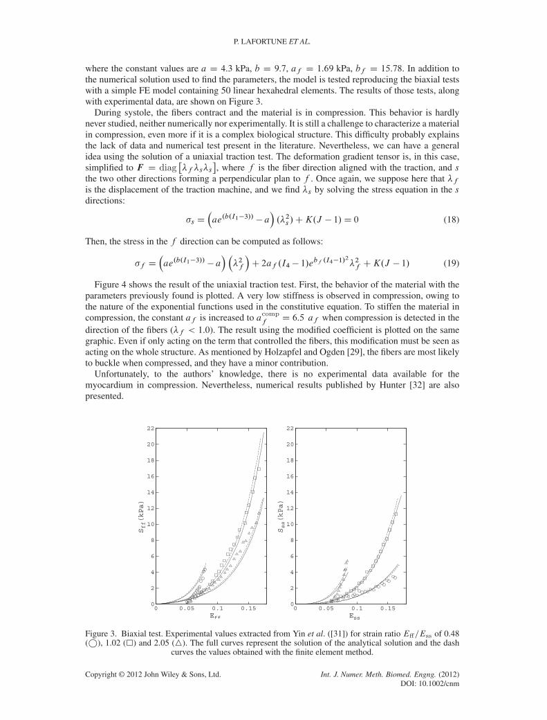
Figure 4 shows the result of the uniaxial traction test. First, the behavior of the material with theparameters previously found is plotted. A very low stiffness is observed in compression, owing tothe nature of the exponential functions used in the constitutive equation. To stiffen the material incompression, the constant af is increased to acomp

fD 6.5 af when compression is detected in the

direction of the fibers (�f < 1.0). The result using the modified coefficient is plotted on the samegraphic. Even if only acting on the term that controlled the fibers, this modification must be seen asacting on the whole structure. As mentioned by Holzapfel and Ogden [29], the fibers are most likelyto buckle when compressed, and they have a minor contribution.

Unfortunately, to the authors’ knowledge, there is no experimental data available for themyocardium in compression. Nevertheless, numerical results published by Hunter [32] are alsopresented.

22

20

18

16

14

12

10

8

6

4

2

00 0.05 0.1 0.15

22

20

18

16

14

12

10

8

6

4

2

0

Sss(kPa)

0 0.05 0.1 0.15Eff Ess

Sff(kPa)

Figure 3. Biaxial test. Experimental values extracted from Yin et al. ([31]) for strain ratio Eff=Ess of 0.48(�), 1.02 (�) and 2.05 (4). The full curves represent the solution of the analytical solution and the dash

curves the values obtained with the finite element method.



50

40

30

20

10

0

-10

-20

-30

-400.8 0.85 0.9 0.95 1 1.05 1.1 1.15 1.2 1.25

σ f (k

Pa)

originalaf modified in compression

Hunter et al.

λf

Figure 4. Solution of the stress equations for a uniaxial tension–compression test. The response given bythe original parameters and when the value of af is modified are shown. Values published by Hunter et al.

[32] are also shown.

2.3. Electromechanical coupling: active tension development

So far, the electrical and mechanical models are described independently and assessed throughindividual tests. The excitation–contraction (EC) coupling is the phenomenon by which the fiberscontract after a wave of electrical activation propagates through the myocardium. EC coupling isthe result of a series of complex reactions that can be summarized as follows. Ca2C enters thecells during the plateau phase of the action potential caused by an increase of the permeability ofthe cell membrane (sarcolemma). This extracellular Ca2C triggers the release of a larger amountof intracellular Ca2C from the sarcoplasmic reticulum. Ca2C then binds to the troponin C, whichinteracts in turn with tropomyosin, allowing the myosin to bind with the actin filaments. Myosinhead pull the actin filament toward the center of the sarcomere, producing the contractile force. Tosimplify, we can say that the free intracellular concentration of Ca2C mediates the contraction of themyocardium, explaining why many models are based on this quantity.

A large amount of EC coupling models have been developed (see [33] for a comprehensivereview). The model used in this study is a ‘one-way coupling’, in which the displacements haveno influence on electrophysiology. Also, it is assumed that the active stress is produced only in thedirection of the fiber. The active contribution is simply summed to passive stress. Then, the totalCauchy stress is expressed by [34]:

� D � pasC �act��,�Ca2C

�f ˝ f (20)

where � pas is the passive stress defined by Equation (14), and f is a unit vector aligned with thefiber in the current configuration. If �f is the muscle fiber stretch and f 0 is the fiber in the referenceconfiguration, it can be expressed by �f f D Ff 0. Hunter and co-workers [32] suggested a simplemodel based on steady state data at different constant levels of activation and extension ratios tocalculate the active stress (see also [35]):

�act D

�Ca2C

n�Ca2C

nCC n50

�max

�1C �

��f � 1

��(21)

where C50 is the value of the intracellular calcium concentration for 50% of �max, n is a coefficientcontrolling the shape of the curve and �max is the maximum isometric active tensile stress developedat �fD1. Experiments show that �max is a linear function of � with � being the non-dimensionalslope dT=d�. This parameter represents the dependence of the force on the sarcomere length. Theforce increases with the stretch of the fiber, because the number of overlapping myosin/actin bendingsite increases. The fluctuation of the free calcium ions concentration follows this relation [36]:�

Ca2C.tloc/D

�Ca2C

max

.tloc=Ca/ exp .1� tloc=Ca/ (22)


P. LAFORTUNE ET AL.

where Ca is a parameter and tloc is the local activation time of a certain integration point of themesh. The tloc is initiate to 0.0 s at the beginning of the simulation for the entire mesh. When themembrane potential overcomes a threshold value (fixed to �50 mV), EC coupling is triggered andtloc starts running at this specific location. Then,

�Ca2C

(and consequently �act) also vary.

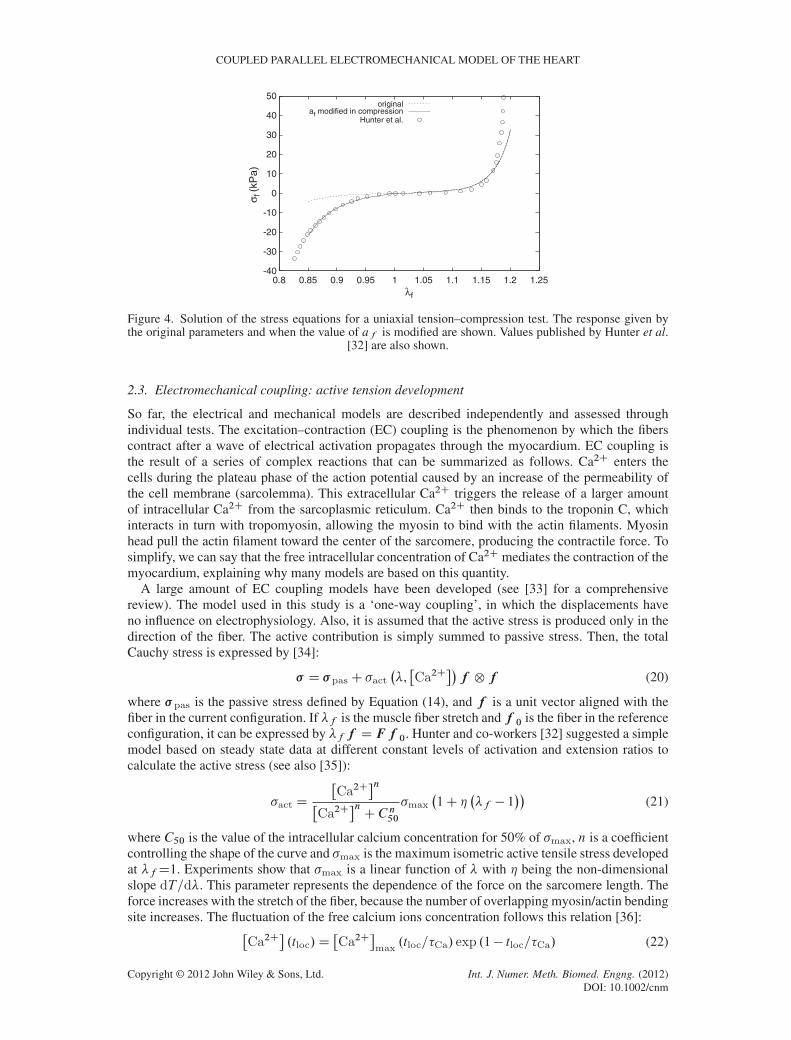
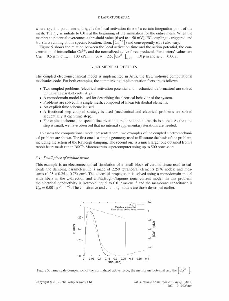
Figure 5 shows the relation between the local activation time and the action potential, the con-centration of intracellular Ca2C, and the normalized active force produced. Parameters’ values areC50 D 0.5 m, �max D 100 kPa, nD 3, �D 2.5,

�Ca2C

maxD 1.0 m and Ca D 0.06 s.

3. NUMERICAL RESULTS

The coupled electromechanical model is implemented in Alya, the BSC in-house computationalmechanics code. For both examples, the summarizing implementation facts are as follows:

� Two coupled problems (electrical activation potential and mechanical deformation) are solvedin the same parallel code, Alya.� A monodomain model is used for describing the electrical behavior of the system.� Problems are solved in a single mesh, composed of linear tetrahedral elements.� An explicit time scheme is used.� A fractional step coupled strategy is used (mechanical and electrical problems are solved

sequentially at each time step).� For explicit schemes, no special linearization is required and no matrix is stored. As the time

step is small, we have observed that no internal supplementary iterations are needed.

To assess the computational model presented here, two examples of the coupled electromechani-cal problem are shown. The first one is a simple geometry used to illustrate the basis of the problem,including the action of the Rayleigh damping. The second one is a much larger one obtained from arabbit heart mesh run in BSC’s Marenostrum supercomputer using up to 500 processors.

3.1. Small piece of cardiac tissue

This example is an electromechanical simulation of a small block of cardiac tissue used to cal-ibrate the damping parameters. It is made of 2250 tetrahedral elements (576 nodes) and mea-sures (0.25 � 0.25 � 0.75) cm3. The electrical propagation is solved using a monodomain modelwith fibers in the ´-direction and a FitzHugh–Nagumo ionic current model. In this problem,the electrical conductivity is isotropic, equal to 0.012ms cm�1 and the membrane capacitance isCm D 0.001F cm�2. The constitutive and coupling models are those described earlier.

-110

-75

-50

-25

0

0 0.05 0.1 0.15 0.2 0.25 0.3 0.35 0.40

0.2

0.4

0.6

0.8

1

1.2

E (

mV

)

[Ca+

+] (

μM)

time (sec)

[Ca++]Membrane potential

Normalized active force

Figure 5. Time scale comparison of the normalized active force, the membrane potential and thehCa2C

i.



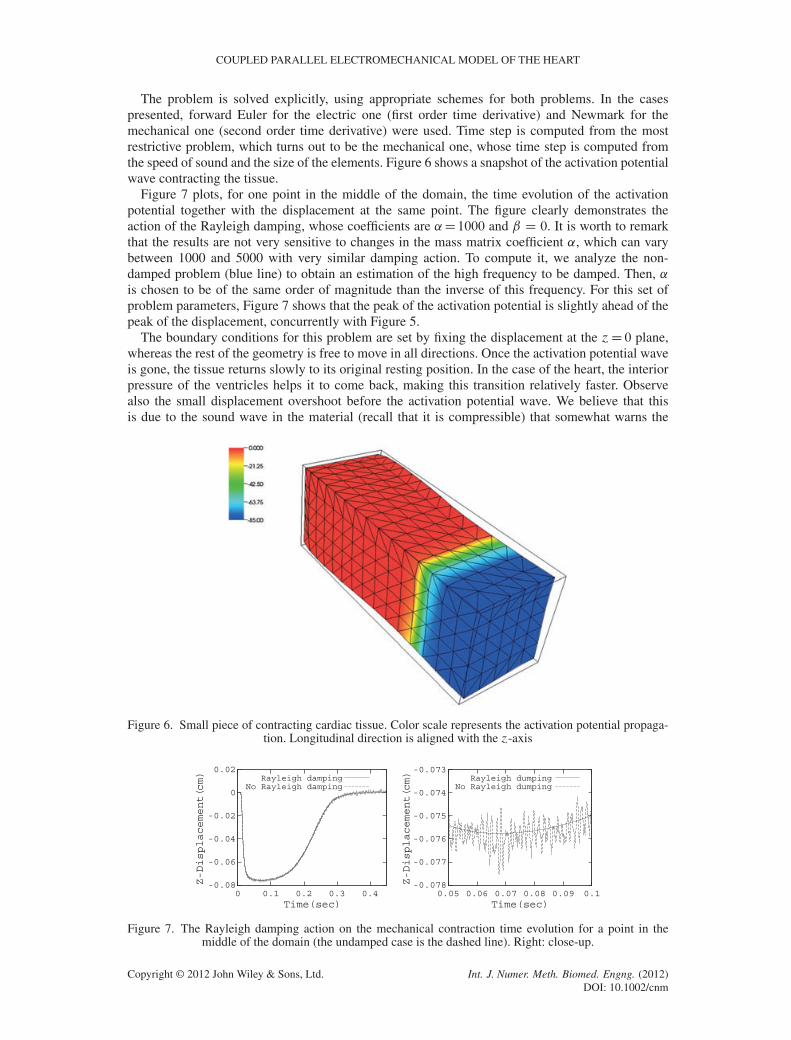
The problem is solved explicitly, using appropriate schemes for both problems. In the casespresented, forward Euler for the electric one (first order time derivative) and Newmark for themechanical one (second order time derivative) were used. Time step is computed from the mostrestrictive problem, which turns out to be the mechanical one, whose time step is computed fromthe speed of sound and the size of the elements. Figure 6 shows a snapshot of the activation potentialwave contracting the tissue.

Figure 7 plots, for one point in the middle of the domain, the time evolution of the activationpotential together with the displacement at the same point. The figure clearly demonstrates theaction of the Rayleigh damping, whose coefficients are ˛D1000 and ˇ D 0. It is worth to remarkthat the results are not very sensitive to changes in the mass matrix coefficient ˛, which can varybetween 1000 and 5000 with very similar damping action. To compute it, we analyze the non-damped problem (blue line) to obtain an estimation of the high frequency to be damped. Then, ˛is chosen to be of the same order of magnitude than the inverse of this frequency. For this set ofproblem parameters, Figure 7 shows that the peak of the activation potential is slightly ahead of thepeak of the displacement, concurrently with Figure 5.

The boundary conditions for this problem are set by fixing the displacement at the ´D 0 plane,whereas the rest of the geometry is free to move in all directions. Once the activation potential waveis gone, the tissue returns slowly to its original resting position. In the case of the heart, the interiorpressure of the ventricles helps it to come back, making this transition relatively faster. Observealso the small displacement overshoot before the activation potential wave. We believe that thisis due to the sound wave in the material (recall that it is compressible) that somewhat warns the

Figure 6. Small piece of contracting cardiac tissue. Color scale represents the activation potential propaga-tion. Longitudinal direction is aligned with the ´-axis

-0.08

-0.06

-0.04

-0.02

0

0 0.1 0.2 0.3 0.4

Z-Displacement(cm) Rayleigh damping

No Rayleigh damping

-0.078

-0.077

-0.076

-0.075

-0.074

0.05 0.06 0.07 0.08 0.09 0.1

Z-Displacement(cm) Rayleigh dumping

No Rayleigh dumping

Time(sec) Time(sec)

-0.0730.02

Figure 7. The Rayleigh damping action on the mechanical contraction time evolution for a point in themiddle of the domain (the undamped case is the dashed line). Right: close-up.


P. LAFORTUNE ET AL.

material points slightly before the activation potential wave arrives. This is a normal behavior ofcompressible flows or deformations.

3.2. Two ventricles of a rabbit heart

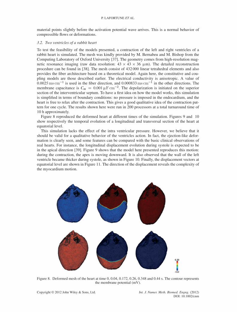
To test the feasibility of the models presented, a contraction of the left and right ventricles of arabbit heart is simulated. The mesh was kindly provided by M. Bernabeu and M. Bishop from theComputing Laboratory of Oxford University [37]. The geometry comes from high-resolution mag-netic resonance imaging (raw data resolution: 43 � 43 � 36 m). The detailed reconstructionprocedure can be found in [38]. The mesh consist of 432 000 linear tetrahedral elements and alsoprovides the fiber architecture based on a theoretical model. Again here, the constitutive and cou-pling models are those described earlier. The electrical conductivity is anisotropic. A value of0.0025ms cm�1 is used in the fiber direction, and 0.000833ms cm�1 in the other directions. Themembrane capacitance is Cm D 0.001F cm�2. The depolarization is initiated on the superiorsection of the interventricular septum. To have a first idea on how the model works, this simulationis simplified in terms of boundary conditions: no pressure is imposed in the endocardium, and theheart is free to relax after the contraction. This gives a good qualitative idea of the contraction pat-tern for one cycle. The results shown here were run in 200 processors at a total turnaround time of10 h approximately.

Figure 8 reproduced the deformed heart at different times of the simulation. Figures 9 and 10show respectively the temporal evolution of a longitudinal and transversal section of the heart atequatorial level.

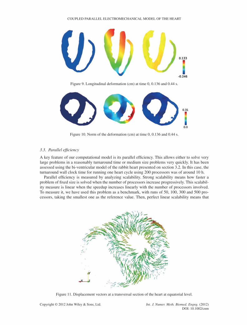
This simulation lacks the effect of the intra ventricular pressure. However, we believe that itshould be valid for a qualitative behavior of the ventricles action. In fact, the ejection-like defor-mation is clearly seen, and some features can be compared with the basic clinical observations ofreal hearts. For instance, the longitudinal displacement evolution during systole is expected to bein the apical direction [39]. Figure 9 shows that the model here presented reproduces this motion:during the contraction, the apex is moving downward. It is also observed that the wall of the leftventricle became thicker during systole, as shown in Figure 10. Finally, the displacement vectors atequatorial level are shown in Figure 11. The direction of the displacement reveals the complexity ofthe myocardium motion.

Figure 8. Deformed mesh of the heart at time 0, 0.04, 0.172, 0.26, 0.348 and 0.44 s. The contour representsthe membrane potential (mV).



Figure 9. Longitudinal deformation (cm) at time 0, 0.136 and 0.44 s.

Figure 10. Norm of the deformation (cm) at time 0, 0.136 and 0.44 s.

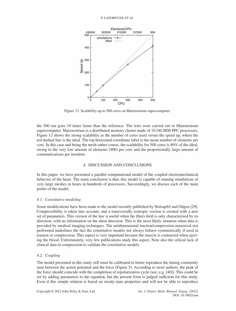
3.3. Parallel efficiency

A key feature of our computational model is its parallel efficiency. This allows either to solve verylarge problems in a reasonably turnaround time or medium size problems very quickly. It has beenassessed using the bi-ventricular model of the rabbit heart presented on section 3.2. In this case, theturnaround wall clock time for running one heart cycle using 200 processors was of around 10 h.

Parallel efficiency is measured by analyzing scalability. Strong scalability means how faster aproblem of fixed size is solved when the number of processors increase progressively. This scalabil-ity measure is linear when the speedup increases linearly with the number of processors involved.To measure it, we have used this problem as a benchmark, with runs of 50, 100, 300 and 500 pro-cessors, taking the smallest one as the reference value. Then, perfect linear scalability means that

Figure 11. Displacement vectors at a transversal section of the heart at equatorial level.


P. LAFORTUNE ET AL.

0

100

200

300

400

500

0 100 200 300 400 500

900107000215000322500430000

Spe

ed U

p

Elements/CPU

simulationsideal

CPU

Figure 12. Scalability up to 500 cores on Marenostrum supercomputer.

the 500 run goes 10 times faster than the reference. The tests were carried out in Marenostrumsupercomputer. Marenostrum is a distributed memory cluster made of 10 240 IBM PPC processors.Figure 12 shows the strong scalability as the number of cores used versus the speed up, where thered dashed line is the ideal. The top horizontal coordinate label is the mean number of elements percore. In this case and being the mesh rather coarse, the scalability for 500 cores is 80% of the ideal,owing to the very low amount of elements (900) per core and the proportionally large amount ofcommunications per iteration.

4. DISCUSSION AND CONCLUSIONS

In this paper, we have presented a parallel computational model of the coupled electromechanicalbehavior of the heart. The main conclusion is that, this model is capable of running simulations ofvery large meshes in hours in hundreds of processors. Succeedingly, we discuss each of the mainpoints of the model.

4.1. Constitutive modeling

Some modifications have been made to the model recently published by Holzapfel and Odgen [29].Compressibility is taken into account, and a transversally isotropic version is created with a newset of parameters. This version of the law is useful when the fibers field is only characterized by itsdirection, with no information on the sheet direction. This is the most likely situation when data isprovided by medical imaging techniques. The unidimensional traction/compression numerical testperformed underlines the fact the constitutive models not always behave symmetrically if used intension or compression. This aspect is very important because the muscle is contracted when eject-ing the blood. Unfortunately, very few publications study this aspect. Note also the critical lack ofclinical data in compression to validate the constitutive models.

4.2. Coupling

The model presented in this study still must be calibrated to better reproduce the timing commonlyseen between the action potential and the force (Figure 5). According to most authors, the peak ofthe force should coincide with the completion of repolarization cycle (see, e.g. [40]). This could beset by adding parameters to the equation, but the present form is judged sufficient for this study.Even if this simple relation is based on steady-state properties and will not be able to reproduce



the realistic velocity-dependent behavior of the myocardium, it is commonly used in finite elementmodel, and it is suitable to simulate the healthy beating heart. If more complex behaviors have to besimulated, a full dynamic model is necessary ([36, 40]).

Coupling from the mechanical to the electrical part is caused by the deformation of the physicalspace, producing a difference in the travel time of the electrical propagation. In this version of themodel, a one-way coupling is used (from electrical to mechanical), and this effect is not considered.It will be taken into account in future works.

4.3. Numerical and implementation issues

All along this paper, we have used explicit schemes for both the mechanical and electrical prob-lems (see [17] for a detailed description of the explicit schemes). Although they are programmedin Alya, owing to the small physical time scales and the high non-linearities of both problems, wehave preferred the all-explicit strategy. From our experience, the staggered loosely coupled strat-egy is specially well-suited for large scale coupled problems. It avoids storing a large matrix witha block for each of the problem and coupling off-diagonal blocks. Besides, it allows the use of themost appropriate numerical solution scheme for each problem block. Regarding the computationalefficiency, it is worth to note that we are far from the optimal. Parallel efficiency is correct, butsequential efficiency must be highly improved. Non-linear solid mechanics of complex materials isexpensive with a large amount of inner nodal or Gauss point loops. Then, one must be very carefulon how these loops are written to stay efficient. As this model is coming out from the initial devel-opment stage, a hard code cleaning must be faced. Based on previous experience, we expect aroundan order of magnitude of improvement.

Another important issue to consider is how much is the relative computational effort of electro-physiolgy and solid mechanics is, especially for large problems. Some researchers propose to usea fine low-order unstructured mesh for solving electrophysiology and a much coarser high-orderstructured one (but not higher than Q2 or Q3) for solid mechanics. In this case, it is usually reportedthat electrophysiology takes more CPU time than solid mechanics (see reviews [2, 41, 42]). Onthe other hand, we propose to use the same unstructured mesh for both problems, which leads tothe opposite ratio. With the models we used for the rabbit ventricles, the figures are around 30%electrophysiology and 70% solid mechanics.

To obtain the results presented here, we have previously performed a set of runs to calibrate theparameters, which can be rather hard. However, some of this parameters have not been explored,but fixed from the beginning; notably, the fibers field and the electrical initial conditions. In theOxford rabbit model, the fibers field comes given based on certain semi-empirical model. On theother hand, we have fixed the initial activation potential to two localized impulses in the basalregion. In this paper, we have preferred to focus on the model itself than studying more advancedphysiological aspects.

4.4. Future lines

Most of the future lines are outlined in the precedent paragraphs. Better and more sophisticate phys-iological models must be included, in the constitutive law, the coupling, the fibers field and theinitial and boundary conditions. Some of these improvements have already been carried out, but arenot the object of this paper. Some others depend on the state of collaboration with bioengineers andmedical doctors. For instance, the model is being used to study infarction and resynchronization.As the model allows to run simulations with high time and space resolution, it is very appealing fordirect validation against experimental measurements on real cases obtained from medical images,such as ejection rate, torsion, wall thickening, deformation time sequence and so on.

ACKNOWLEDGEMENTS

This work is made possible, thanks to the close collaboration with bio-engineers and medical doctors.Among them are D. Gil and J. Garcia-Barnés (Computer Vision Center CVC-UAB, Spain), F. Carreras(Htal. de Sant Pau, Spain), M. Ballester Rodés (U. Lleida, Spain), A. Jerusalém and D. Tjahjanto (IMDEA

Copyright © 2012 John Wiley & Sons, Ltd.DOI: 10.1002/cnm

Int. J. Numer. Meth. Biomed. Engng. (2012)

P. LAFORTUNE ET AL.

Materials, Spain), D. Auger and T. Franz (Univ. of Cape Town, South Africa) and M. Bernabeu and M.Bishop (Oxford University, UK).

REFERENCES

1. Nordsletten DA, Niederer SA, Nash MP, Hunter PJ, Smith NP. Coupling multi-physics models to cardiac mechanics.Progress in Biophysics and Molecular Biology 2011; 104(1-3):77–88.

2. Trayanova N, Winslow R. Whole heart modeling. Applications to cardiac electrophysiology and electromechanics.Circulation Research 2011; 108(4):113–128.

3. Nickerson D, Smith N, Hunter PJ. New developments in a strongly coupled cardiac electromechanical model.Europace 2005; 7:118–127.

4. Sainte-Marie J, Chapelle D, Cimrman R, Sorine M. Modeling and estimation of the cardiac electromechanicalactivity. Computers and Structures 2006; 84:1743–1759.

5. Stevens C, Remme E, LeGrice I, Hunter P. Ventricular mechanics in diastole: Material parameter sensitivity. Journalof Biomechanics 2003; 36(5):737–748.

6. Göktepe S, Kuhl E. Electromechanics of the heart: A unified approach to the strongly coupled excitation-contractionproblem. Computational Mechanics 2010; 45:227–243.

7. Kerckhoffs RCP, Neal M, Gu Q, Bassingthwaighte JB, Omens J, McCulloch A. Coupling of a 3D finite elementmodel of cardiac ventricular mechanics to lumped systems models of the systemic and pulmonic circulation. Annalsof Biomedical Engineering 2007; 35:1–18.

8. Nobile F, Quarteroni A, Ruiz-Baier R. An active strain electromechanical model for cardiac tissue. InternationalJournal for Numerical Methods in Biomedical Engineering 2011. DOI: 10.1002/cnm.1468.

9. Gurev V, Constantino J, Rice JJ, Trayanova NA. Distribution of electromechanical delay in the heart: Insights froma three-dimensional electromechanical model. Biophysical Journal 2010; 99(3):745–754.

10. Hosoi A, Washio T, Okada J, Kadooka Y, Nakajima K, Hisada T. A multi-scale heart simulation on massively par-allel computers. In Proceedings of the 2010 ACM/IEEE International Conference for High Performance Computing,Networking, Storage and Analysis, SC ’10. IEEE Computer Society: Washington, DC, USA, 2010; 1–11.

11. Reumann M, Fitch BG, Rayshubskiy A. et al. Strong scaling and speedup to 16,384 processors in cardiac electromechanical simulations. Engineering in Medicine and Biology Society, 2009. EMBC 2009. Annual InternationalConference of the IEEE, Minneapolis, Minnesota, USA, september 2009; 2795–2798.

12. Vázquez M, Arís R, Houzeaux G. et al.A massively parallel computational electrophysiology model of the heart.International Journal for Numerical Methods in Biomedical Engineering 2011. DOI: 10.1002/cnm.1443.

13. Houzeaux G, Aubry R, Vázquez M. Extension of fractional step techniques for incompressible flows: Thepreconditioned orthomin(1) for the pressure schur complement. Computers and Fluids 2011; 44:297–313.

14. Available from: http://www.bsc.es..15. FitzHugh RA. Impulses and physiological states in theoretical models of nerve membrane. Journal of Biophysics

1961; 1:445–466.16. Fenton FH, Cherry EM, Karma A, Rappel W. Modeling wave propagation in realistic heart geometries using the

phase-field method. Chaos 2005; 15(013502).17. Belytschko T, Liu WK, Moran B. Nonlinear Finite Elements for Continua and Structures. John Wiley and Sons:

Chichester, 2000.18. Yin FC, Chan CC, Judd RM. Compressibility of perfused passive myocardium. American Journal of Physiology -

Heart and Circulatory Physiology 1996; 271(H1864-H1870).19. Moore CC, McVeigh ER, Elias AZ. Noninvasive measurement of three-dimensional myocardial deformation with

tagged magnetic resonance imaging during graded local ischemia. Journal of Cardiovascular Magnetic Resonance1999; 1(3):207–222.

20. Legrice I, Hunter P, Young A, Smaill B. The architecture of the heart: A data–based model. PhilosophicalTransactions of the Royal Society of London. Series A: Mathematical, Physical and Engineering Sciences 2001;359(1783):1217–1232.

21. Streeter DD, Powers WE, Ross MA, Torrent-Guasp F. Three-dimensional fiber orientation in the mammalian leftventricular wall. In Cardiovascular System Dynamics, Barn J, Noordegraf A, Raines J (eds). MIT Press: Cambridge,MA, 1978; 73.

22. Dokos S, Smaill BH, Young AA, LeGrice IJ. Shear properties of passive ventricular myocardium. American Journalof Physiology - Heart and Circulatory Physiology 2002; 283(6):H2650–2659.

23. Watanabe H, Sugiura S, Kafuku H, Hisada T. Multiphysics simulation of left ventricular filling dynamics usingfluid-structure interaction finite element method. Biophysical Journal 2004; 87(3):2074–2085.

24. Veress AI, Segars WP, Weiss JA, Tsui BMW, Gullberg GT. Normal and pathological ncat image and phantom databased on physiologically realistic left ventricle finite-element models. IEEE Transactions on Medical Imaging 2006;25(12):1604–1616.

25. Dorri F, Niederer PF, Lunkenheimer PP. A finite element model of the human left ventricular systole. ComputerMethods in Biomechanics and Biomedical Engineering 2006; 9(5):319–341.

26. Kerckhoffs RCP, Healy SH, Usyk TP, McCulloch AD. Computational methods for cardiac electromechanics.Proceedings of the IEEE April 2006; 94(4):769–783.



27. Costa KD, Holmes JW, McCulloch AD. Modelling cardiac mechanical properties in three dimensions. Philosophi-cal transactions of the Royal Society of London. Series A: Mathematical, physical and engineering sciences 2001;359(1783):1233–1250.

28. Holzapfel GA. Nonlinear Solid Mechanics: A Continuum Approach for Engineering. John Wiley and Sons:Chichester, 2000.

29. Holzapfel GA, Ogden RW. Constitutive modelling of passive myocardium: A structurally based framework for mate-rial characterization. Philosophical Transactions of the Royal Society A: Mathematical, Physical and EngineeringSciences 2009; 367(1902):3445–3475.

30. Usyk TP, Mazhari R, McCulloch AD. Effect of laminar orthotropic myofiber architecture on regional stress andstrain in the canine left ventricle. Journal of Elasticity 2000; 61:143–164.

31. Yin FC, Strumpf RK, Chew PH, Zeger SL. Quantification of the mechanical properties of noncontracting caninemyocardium under simultaneous biaxial loading. Journal of Biomechanics 1987; 20(6):577–589.

32. Hunter PJ, Nash MP, Sands GB. Computational Electromechanics of the Heart, Computational Biology of the Heart.John Wiley and Sons: London, 1997. 346–407.

33. Rice JJ, de Tombe PP. Approaches to modeling crossbridges and calcium-dependent activation in cardiac muscle.Progress in Biophysics and Molecular Biology 2004; 85(2-3):179–195.

34. Humphrey JD. Cardiovascular Solid Mechanics. Cells, Tissues, and Organs. Springer: New York, NY, 2001.35. Holzapfel GA. Computational Biomechanics of Soft Biological Tissue, Volume 2 of Encyclopedia Of Computational

Mechanics. John Wiley & Sons: Chichester, 2004. Chapter 18, 604–635.36. Hunter PJ, McCulloch AD, ter Keurs HEDJ. Modelling the mechanical properties of cardiac muscle. Progress in

Biophysics and Molecular Biology 1998; 69:289–331.37. Computing Laboratory. Oxford University. Available from: http://www.cs.ox.ac.uk/chaste.38. Bishop MJ, Plank G, Burton RAB, Schneider JE, Gavaghan DJ, Grau V, Kohl P. Development of an anatomically

detailed MRI-derived rabbit ventricular model and assessment of its impact on simulations of electrophysiologicalfunction. American Journal of Physiology - Heart and Circulatory Physiology 2010; 298(2):H699–H718.

39. Moore CC, Lugo-Olivieri CH, McVeigh ER, Zerhouni EA. Three-dimensional systolic strain patterns in the normalhuman left ventricle: Characterization with tagged mr imaging. Radiology 2000; 214(2):453–466.

40. Rice JJ, Wang F, Bers DM, de Tombe PP. Approximate model of cooperative activation and crossbridge cycling incardiac muscle using ordinary differential equations. Biophysical journal 2008; 95(5):2368–2390.

41. Trayanova N, Eason J, Aguel F. Computer simulations of cardiac defibrillation: A look inside the heart. Computingand Visualization in Science 2002; 4:259–270.

42. Trayanova N, Rice JJ. Cardiac electromechanical models: From cell to organ. Frontiers in Physiology 2011; 2(0).


Coupled electromechanical model of the heart: Parallel finite element formulation

Documents

Transcript of Coupled electromechanical model of the heart: Parallel finite element formulation