Coupled Dynamic–Thermodynamic Forcings during Tropical Cyclogenesis.Part II: Axisymmetric Experiments

BRIAN H. TANG

Department of Atmospheric and Environmental Sciences, University at Albany, State University of

New York, Albany, New York

(Manuscript received 16 February 2017, in final form 25 April 2017)

ABSTRACT

An ensemble of axisymmetric model experiments with simplified physics is used to evaluate the diagnostic

framework presented in Part I. The central piece of the framework is understanding what causes decreases in

the ratio of bulk differences of moist entropy over differences of angular momentum between two defined

regions, the boundary between the two demarcating the approximate location of the emergence of the radius

of maximum wind of the developing meso-beta-scale protovortex. Within a day before tropical cyclogenesis,

the moist entropy forcing results in a decrease of this ratio. Net advective fluxes act to export moist entropy

from the outer region and import moist entropy into the inner region, resulting in a positive radial gradient in

gross moist stability that is maximized around the time of genesis. While surface moist entropy fluxes are

needed for genesis to occur, they act synergistically with the net advective fluxes to decrease the ratio before

and during genesis. Within a day after tropical cyclogenesis, surface moist entropy fluxes directly amplify the

positive difference in moist entropy between the inner and outer regions, and radial fluxes of angular mo-

mentum reduce the magnitude of the negative difference in angular momentum between the inner and outer

regions. Both of these processes act to reduce the ratio further. The framework highlights differences in

processes occurring before, during, and after genesis as the meso-beta-scale protovortex develops and

intensifies.

1. Introduction

There exist multiscale dynamical and thermodynam-

ical components that must be considered in combination

to understand tropical cyclogenesis. A few key compo-

nents before and during tropical cyclogenesis are the

moistening of a meso-beta-scale deep-tropospheric re-

gion in the inner region of a tropical disturbance (Bister

and Emanuel 1997; Raymond et al. 1998, 2011; Davis

and Ahijevych 2012; Wang 2012; Komaromi 2013;

Zawislak and Zipser 2014), the increasing depth and

amplitude of the warm core (Dolling and Barnes 2012;

Zhang and Zhu 2012; Cecelski and Zhang 2013; Kerns

and Chen 2015), and the formation of the meso-beta-

scale, low-level protovortex within the larger meso-

alpha-scale circulation (Nolan 2007; Dunkerton et al.

2009; Wang et al. 2010; Montgomery et al. 2012; Lussier

et al. 2014; Wang 2014; Kilroy et al. 2017).

Tang (2017, hereafter Part I) introduced a coupled

dynamic–thermodynamic diagnostic framework that allows

for the investigation of processes responsible for the de-

velopment of these components. The key metric x is

defined as the ratio of bulk differences in moist entropy

Ds over bulk differences in angular momentum DM be-

tween an inner and outer region (Fig. 1a). The inner cy-

lindrical region has a radius of ri, and the outer annular

region extends from ri to ro. Both regions have a height of

zt. The time tendency of x is of particular relevance:

›x

›t5

a

DM

›

›t(Ds)|fflfflfflfflfflfflfflffl{zfflfflfflfflfflfflfflffl}

ss

2aDs

(DM)2›

›t(DM)|fflfflfflfflfflfflfflfflfflfflfflffl{zfflfflfflfflfflfflfflfflfflfflfflffl}

sM

, (1)

where a is a nondimensionalization factor (see Part I),

ss is the moist entropy forcing, and sM is the angular

momentum forcing. Moistening and the amplification of

the warm core within the inner region at a greater rate

than the outer region results in a more positive Ds andmore negative x, because DM must be negative in order

for the vortex to be inertially stable. Concentrating an-

gular momentum in the inner region at a faster rate than

the outer region, as the protovortex spins up and theCorresponding author: Brian H. Tang, btang@albany.edu

JULY 2017 TANG 2279

DOI: 10.1175/JAS-D-17-0049.1

� 2017 American Meteorological Society. For information regarding reuse of this content and general copyright information, consult the AMS CopyrightPolicy (www.ametsoc.org/PUBSReuseLicenses).

radius of maximum wind begins to contract inward in

the inner region, resulting in a less negative DM and a

more negative x. It is therefore reasonable to postulate

that a decrease in x signifies tropical cyclogenesis is

occurring, but what is the character of this decrease (i.e.,

more gradual versus abrupt)? What is the relative

importance of changes in Ds and/or DM toward de-

creasing x before, during, and after genesis?

A principle advantage of using moist entropy and

angular momentum is that their budgets can be easily

quantified over both the inner and outer regions

(Fig. 1b), thereby allowing ss and sM to be expanded:

ss5

a

DM

�2

�1

mi

11

mo

�ðzt0

ð2p0

(u2 _ri)rsrj

ridudz1

1

mo

ðzt0

ð2p0

(u2 _ro)rsrj

rodu dz

21

mi

ð2p0

ðri0

wrsjztr dr du1

1

mo

ð2p0

ðrori

wrsjztr dr du

11

mi

ð2p0

ðri0

Fnets r dr du2

1

mo

ð2p0

ðrori

Fnets r dr du

#(2)

and

sM5

aDs

(DM)2

��1

mi

11

mo

�ðzt0

ð2p0

(u2 _ri)rMrj

ridudz2

1

mo

ðzt0

ð2p0

(u2 _ro)rMrj

rodu dz

11

mi

ð2p0

ðri0

wrMjztr dr du2

1

mo

ð2p0

ðrori

wrMjztr dr du

21

mi

ð2p0

ðri0

FMjz50

r dr du11

mo

ð2p0

ðrori

FMjz50

r dr du

#, (3)

where mi is the mass of the inner region, mo is the mass

of the outer region, u is the radial wind, w is the vertical

wind, _ri and _ro are the time rates of change of ri and ro(see Part I), r is the dry density, Fnet

s is the net column

nonadvective flux of moist entropy, and FM is boundary

fluxes of angular momentum. See Part I for explanations

of the terms. Equations (2) and (3) allow one to assess

which processes are important to changing x and when.

FIG. 1. (a) A planar view of a hypothetical tropical disturbance. The inner cylindrical region

extends to ri, and the outer annular region extends from ri to ro. Both regions extend from the

surface to zt . (b) Moist entropy and angular momentum budgets in each region. Purple arrows

are radial advective fluxes through ri and ro, green arrows are vertical advective fluxes through zt ,

orange arrows are radiative fluxes of moist entropy at zt , red arrows are surface fluxes of moist

entropy, and blue arrows are surface fluxes of angular momentum. Figure is adapted from Part I.

2280 JOURNAL OF THE ATMOSPHER IC SC IENCES VOLUME 74

For example, a net advective flux of moist entropy from

the outer to inner regions might yield a negative ss,

decreasing x. Larger surface enthalpy fluxes in the inner

region compared to the outer region might also yield a

negative ss. Likewise, one may obtain similar relation-

ships between sM and its components.

Differences in the net advective flux of moist entropy

in the inner and outer regions serve as a bulk metric of

radial gradients of the gross moist stability (GMS),

provided there is mean ascent in both the inner and

outer regions. While a lower GMS has been hypothe-

sized to favor bottom-heavy convective mass flux pro-

files that quickly spin up the low-level vortex (Raymond

and Sessions 2007; Raymond et al. 2007, 2014), the role

of radial gradients and the time evolution of the GMS

around tropical cyclogenesis remain to be investigated.

We will apply the framework in a set of axisymmetric

hurricane model experiments. Section 2 describes the

modeling methodology. Section 3 explains how genesis

is defined in the experiments. Section 4 analyzes the

experiments using the framework. Section 5 ends with

conclusions.

2. Methodology

a. Model

The model used in this study is the Axisymmetric

Simplified Pseudoadiabatic Entropy Conserving Hurri-

cane (ASPECH) model (Tang and Emanuel 2012,

hereafter TE12), a nonhydrostatic model phrased in

radius–height coordinates. The domain extends to

1500km in radius and 25 km in height. The radial grid

spacing is 2 km, and the vertical grid spacing is 0.3 km.

The Coriolis parameter is fixed at 5.0 3 1025 s21. A

simple set of parameterizations is used. Radiation is

parameterized through a constant radiative cooling rate

of 22K day21 in the troposphere, which is typical for

clear-sky conditions in the tropics (Hartmann et al.

2001). There are no cloud–radiative feedbacks. Micro-

physics is parameterized using the Kessler scheme

(Kessler 1969) with a constant terminal velocity for rain

of 27ms21. Turbulence is parameterized using the

methodology of Bryan and Rotunno (2009), except us-

ing the fully compressible equations. Surface fluxes are

parameterized using bulk aerodynamic formulas. The

enthalpy exchange coefficient is fixed at 1.23 1023, and

the drag coefficient is fixed at 1.5 3 1023, which are

approximate values at surface wind speeds between 10

and 20ms21 (Black et al. 2007). There is no convective

parameterization. The purpose of using a simple set of

parameterizations is to reduce the degrees of freedom in

the model to test the essence of the framework.

ASPECH is a finite-volume model and fully conser-

vative in the absence of boundary sources and sinks.

Moist entropy and angular momentum are prognostic

variables. The conservative nature of the model allows

for an accurate accounting of the components of ss and

sM, which would otherwise potentially have large re-

siduals for a model that uses numerical methods that are

approximately conservative or does not have a prog-

nostic moist entropy equation. Details of the numerical

methods of ASPECH are given in TE12.

b. Initial conditions

The model is initialized with a balanced vortex that

has a maximum tangential wind of 10ms21 at 100-km

radius and 5-km height (Fig. 2). The radial structure of

the vortex is specified using (6) from Knaff et al. (2011)

with a radius of zero wind of 500km. The vertical struc-

ture is the square root of a half cosine profile, such that

the vortex vanishes above 12km. The initial maximum

tangential wind at the surface is about 6ms21. Angular

momentum contours bow inward where the tangential

wind is positive, reaching their apex at 5-km height.

The temperature and moisture profiles are initialized

with the Dunion (2011) moist tropical sounding. The

temperature and moisture are adjusted to be in thermal-

wind balance with the vortex, adapted from the pro-

cedure of Smith (2006), such that the relative humidity is

constant with radius. Positive moist entropy perturba-

tions exist above 5 km, while negative moist entropy

perturbations exist below 5km within 300 km.

An ensemble of 20 experiments is generated by add-

ing uniformly distributed, random perturbations to the

initial water vapor mixing ratio in the lowest three

FIG. 2. Initial tangential wind (shaded; m s21), horizontal moist

entropy perturbations (black contours; every 2.5 J kg21K21 with

negative values dashed and zero line omitted), and angular momen-

tum (red contours; every 106m2 s21 beginning at 0.1 3 106m2 s21).

JULY 2017 TANG 2281

model levels, similar to the methodology of Van Sang

et al. (2008). The perturbations are randomly drawn

from a uniform distribution between 21 and 11 g kg21

with a mean of zero and are different for each experi-

ment. Small differences in the initial condition generate

spread in the spinup evolution in the experiments. The

spread is fundamental to the stochastic nature of con-

vection and its upscale effects on the circulation (Zhang

and Sippel 2009; Tang et al. 2016). An ensemble average

filters out a portion of the stochastic component,

yielding a higher signal-to-noise ratio.

3. Genesis interval

It is convenient to have some objective measure of

genesis time. We define an objective genesis time in

ASPECH based on three threshold conditions that must

bemet for all 6-h periods subsequent to the genesis time.

Each threshold condition has a range, yielding a large

number of possible genesis times, acknowledging that

tropical cyclogenesis is a continuous, nonmonotonic

process that does not lend itself well to a single univar-

iate threshold.

The first condition is that the 6-h average 10-m max-

imumwind speed y10mmust exceed a value ranging from

10 to 15ms21. While there is no explicit minimum in-

tensity required for a tropical depression (American

Meteorological Society 2012), this range encompasses

typical operational intensities of tropical depressions

and is larger than the initial maximum wind speed at the

surface. The second condition is that the standard de-

viation of r80, the innermost radius at which the 10-m

wind speed equals 80% the 10-m maximum wind speed

(Nguyen et al. 2014), must be less than a value ranging

from 15 to 30km. The advantage of using r80 over the

radius of maximum wind is that r80 is a more stable

metric for weak, flat radial wind profiles. This condition

requires there to be coherence in the vortex, associated

with the formation of a compact vortex that is sub-

sequently sustained within the broader circulation

(Nolan 2007). The third condition is that themode of z80,

the lowest height at which the wind equals 80% the

maximum wind speed anywhere in the domain, must be

less than a value ranging from 1 to 2.5 km. The vortex

should have its maximum amplitude at low levels, which

is a defining characteristic of a tropical cyclone.

Each range for the three conditions is divided into 10

values, yielding 1000 genesis times when considering all

possible combinations. The minimum and maximum of

the genesis times defines a genesis interval. The genesis

interval accounts for uncertainty in the genesis time in a

robust manner, but it should be noted that any criteria

for genesis will be arbitrary to some degree. Themean of

the genesis times for each experiment will serve as an

anchor point for compositing, and we will call this mean

the ‘‘genesis time’’ for simplicity.

Figure 3 shows Hovmöller diagrams of y10m, r80, and

z80 for a sample of experiments. Through the first day,

y10m mostly remains under 10ms21 and then varies

around 10ms21 up to the start of the genesis interval.

Before genesis, there is relatively large variability in r80that is tied to transient features that propagate radially

inward. There are also short periods where the vortex is

strongest above 2.5 km, but z80 is predominately at or

below 1km. The lack of longer periods where the mid-

level vortex is stronger than the low-level vortex is likely

due to the lack of ice microphysics, which is important

for stratiform precipitation and the resulting midlevel

inflow that spins up the midlevel vortex (Grabowski

2003). Through the genesis interval, there is a trend to-

ward intensification of the vortex and a consolidation of

r80 around 100 km. After the genesis interval, the vortex

continues to intensify and r80 generally contracts inward.

The genesis time ranges from 64 to 85h in the ensemble

of experiments (Fig. 4). The spread is representative of the

stochastic effects of convection and ranges for the three

conditions, representing the uncertainty in genesis times

in ASPECH. The genesis interval width for each indi-

vidual experiment varies from a few hours (Fig. 3a) to

about a day (Fig. 3c), indicating a spectrum of abrupt to

gradual developments. The mean genesis interval width is

about 12h.

Figures 5a, 5d and 5g show the composite ensemble-

mean structure 0–24h prior to the start of the genesis

interval. The vortex has a broad area of winds between 10

and 12.5ms21 in the lower half of the troposphere. The

angular momentum contours have moved inward in the

lower troposphere compared to their initial position

(Fig. 2). Furthermore, the initial negative moist entropy

perturbations have decayed and switched to positive

moist entropy perturbations within 300km, reaching a

maximum of greater than 25 Jkg21K21 at 4 km in height

and 100km in radius.

Themoist entropy perturbations can be divided into the

part due to potential temperature perturbations and the

part due to moisture perturbations. Most of the positive

moist entropy perturbations are due to moisture pertur-

bations (Fig. 5g), although a weak warm core is beginning

to develop (Fig. 5d) before the genesis interval.

During the genesis interval (Figs. 5b,e,h), the vortex

has intensified further with a sharper radial peak in the

tangential winds between 100 and 150 km, where the

maximum tangential winds have increased to greater

than 15ms21 around 1–2km in height. The sharper ra-

dial peakmarks the formation of a more coherent radius

of maximum wind, as inferred by the decrease in

2282 JOURNAL OF THE ATMOSPHER IC SC IENCES VOLUME 74

variance in r80 during the genesis interval (Fig. 3). The

radial angular momentum gradient in the lower tropo-

sphere also increases as angular momentum contours

move inward. Additionally, the positive moist entropy

perturbations have increased in magnitude to greater

than 30 J kg21K21 as a result of continued increases in

the moisture perturbations (Fig. 5h). The positive moist

entropy perturbations also increase in areal extent, as

the warm core strengthens inward of 150 km (Fig. 5e).

Within the 24h after the end of the genesis interval

(Fig. 5c), the vortex intensifies further, and the radius of

maximum wind contracts inward. The radial gradient of

angular momentum increases, particularly on the radi-

ally inward side of the radius of maximum wind. In this

same region, the moist entropy perturbations continue

to increase, reaching amaximumgreater than 35Jkg21K21.

The depth of the positive moist entropy perturbations

also grows as a result of the amplifying warm core

(Fig. 5f), consistent with the early stages of the devel-

opment of the warm-core structure in 3D model simu-

lations (Stern andNolan 2012). The increase in themoist

entropy perturbation magnitude and depth is consistent

with composite dropsonde observations around genesis

(Zawislak and Zipser 2014).

Figure 5 paints a complex evolution of the moist en-

tropy and angular momentum fields. We now use the

diagnostic framework to investigate the roles of the

moist entropy and angular momentum forcing compo-

nents around tropical cyclogenesis.

4. Framework evaluation

The framework requires specification of initial values

of ri, ro, and zt. As explained in Part I, ri is chosen to

FIG. 3. Hovmöller diagrams of y10m, r80, and z80 for the experiment with (a) the earliest genesis interval, (b) the

latest genesis interval, and (c) the longest genesis interval. The value of r80 is given along the abscissa. Dashes, dots,

and plus signs indicate z80 is below 1.0 km, between 1.0 and 2.5 km, and above 2.5 km in height, respectively. The

color shading of each symbol gives y10m (m s21) according to the scale. The light blue shading is the genesis interval,

and the thick dashed line is the mean genesis time.

FIG. 4. Cumulative distribution of the genesis interval bounds

(light blue shading) and the mean genesis time (black line) for all

the experiments.

JULY 2017 TANG 2283

be the approximate location where the low-level ra-

dius of maximum wind emerges in order to under-

stand processes around the emerging meso-beta-scale

protovortex. The ensemble-mean radius of maximum

10-m wind is 125 km during the genesis interval, with

80% of the experiments lying between 100 and 150 km

(not shown). Note that this choice of ri is particular

to this set of ASPECH experiments and would likely

FIG. 5. (a)–(c) Composite ensemble-mean tangential wind (shaded; m s21), horizontal moist entropy perturbations (black contours;

every 5 J kg21 K21 with negative values dashed and zero line omitted), and angular momentum (red contours; every 106m2 s21 beginning

at 0.1 3 106m2 s21). (d)–(f) Black contours are the potential temperature component of the horizontal moist entropy perturbations

(additional thin contour is 12.5 J kg21 K21). (g)–(i) Black contours are the moisture component of the horizontal moist entropy per-

turbations. Time averages are (a),(d),(g) 24-h period prior to the start of the genesis interval; (b),(e),(h) genesis interval; and (c),(f),(i) 24-h

period after the end of the genesis interval.

2284 JOURNAL OF THE ATMOSPHER IC SC IENCES VOLUME 74

be different for other initial conditions or model

experiments.

To test how the choice of initial ri and ro affects the

behavior of x, we choose the initial ri to be 100, 125, or

150km and the initial ro to be 175, 200, or 225 km.We fix

zt at 17 km, just above the height of the initial tropopause,

such that the full secondary circulation is captured. The

combinations of ri and ro yield nine possible domains.

For each experiment and domain, x is calculated.A low-

pass finite impulse response filter is then applied to remove

high-frequency variability at periods less than half a day to

filter out unbalanced ‘‘noise,’’ since a key assumption of

the framework is that the azimuthal-average vortex above

the boundary layer is nearly in balance on time scales

greater than half a day. The experiments are then com-

posited relative to their individual genesis times. Unless

otherwise stated, all figures hereafter show low-pass-

filtered and composited variables.

Figure 6 shows the ensemble mean x for the nine

different domains. As ri increases for fixed ro (from blue,

to black, to red lines for a fixed line style), x decreases.

As the inner region gets larger, it encompasses a greater

portion of the most positive moist entropy anomalies

(Fig. 5), resulting in an increase in Ds. As ro increases for

fixed ri (from dashed, to solid, to dotted lines for a fixed

color), x also decreases. As the outer region gets larger,

it encompasses a greater portion of the smaller moist

entropy anomalies. As a result, Ds also increases with

increasing ro. In the limit the outer region extends to

very large radius, the outer region would effectively

represent the environment. Having too large of an

outer or inner region would render the framework less

useful, as it would lack resolution of processes occurring

around the radius of maximum wind of the developing

protovortex. Having too small of an outer or inner re-

gion could violate the assumption that the regions exist

in a quasi-balanced state and potentially lead to in-

creased unbalanced noise. Note that DM is also affected

by the choice of ri and ro, but the nondimensionalization

factor a eliminates the sensitivity (see Part I). Addition-

ally, there is little sensitivity in x when varying zt from the

middle troposphere to lower stratosphere (not shown).

Even though the magnitude and sign of x are sensitive

to the initial choice of ri and ro, there are common traits in

the evolution of x across all the domains. The curves in

Fig. 6 roughly parallel each other. Before the genesis in-

terval, x is either flat or slowly decreasing. Themagnitude

of x generally remains below 1.0, indicating that the

magnitude of DsDM21 is less than or equal to a21, the

chosen reference value. After the genesis interval, x is

clearly decreasing at a much faster rate than before the

genesis interval. The genesis interval itself represents a

transition period.

Hereafter, we only analyze the domain with an initial

ri of 125km and ro of 200 km. This domain has a ri near

the ensemble mean radius of maximum 10-m wind.

Figure 7 shows the evolution of x for the individual

experiments and the ensemble mean. The ensemble

mean dampens the variability seen in each experiment.

While there is a tendency for a slow decrease before the

start of the genesis interval, most of the experiments

have oscillations between21.0 and 0.5. The oscillations

in x are inferred to be the manifestation of convective

FIG. 6. Composite ensemble-mean time series of the low-pass-

filtered x for combinations of three initial ri and three initial ro,

given in the legend (km). The light blue shaded area here and in all

subsequent figures is the mean genesis interval.

FIG. 7. As in Fig. 6, but for only an initial ri 5 125 km and ro 5200 km. The thin, gray lines denote each experiment, and the thick

black line denotes the ensemble mean.

JULY 2017 TANG 2285

bursts modifying the moist entropy and, to a lesser extent,

the angular momentum in each region. Within the genesis

interval or shortly after, x in almost all of the experiments

begins to sharply decrease. The key question is what pro-

cesses are responsible for the decrease in x.

The decrease in x is investigated by taking the time

tendency of x over a moving 6-h window and calculating

ss and sM over the same window (Fig. 8). Before220h,

the time tendency of the ensemble mean of x is near

zero. The ensemble-mean moist entropy and angular

momentum forcing components are also near zero, but

the moist entropy forcing shows much greater ensemble

spread. After 220h, the time tendency of x decreases

as a result of a concomitant decrease in the moist en-

tropy forcing. Over the same period, the angular mo-

mentum forcing increases slightly but remains near zero.

After the genesis time, the angular momentum forcing

becomes negative and decreases sharply thereafter,

surpassing the magnitude of the moist entropy forcing

about 15 h after the genesis time. Meanwhile, the moist

entropy forcing increases, but still generally remains

negative, consistent with the expansion of the high-

entropy core (Fig. 5c). Hence, in the period from 212h

to the end of the genesis interval, the decrease in x is

largely dominated by the moist entropy forcing. After

the genesis interval, the moist entropy forcing and an-

gular momentum forcing are both important, but the

angular momentum forcing has an increasing role in

further decreasing x.

Figure 9 shows the components of the moist entropy

forcing, the rhs of (2). The first pair of terms on the rhs of

(2) represent the radial advective flux component, and

the second pair of terms represent the vertical advective

flux component. The largest components are the radial

advective flux and the vertical advective flux (Fig. 9a).

The two nearly cancel each other out, making it im-

portant to have accurate and high-time-resolution out-

put of the advective fluxes. Figure 9a also indicates

vertical fluxes of moist entropy at the domain top are

large and cannot be neglected, at least in this model and

these experiments. This result applies even if zt is

moved upward.

The radial and vertical advective flux components are

combined to yield a total advective flux (Fig. 9b). Ad-

ditionally, the surfacemoist entropy flux component and

FIG. 8. Composite ensemble-mean time series of the low-pass-

filtered time tendency of x (black line), moist entropy forcing (blue

line), and angular momentum forcing (red line). Shaded areas give

the interquartile range of the moist entropy forcing and angular

momentum forcing.

FIG. 9. Composite ensemble-mean time series of the low-pass-filtered moist entropy forcing components:

(a) radial (purple) and vertical (green) advective fluxes; (b) total advective flux (black), surface moist entropy flux

(maroon), radiative flux (orange), and moist entropy forcing (blue). Shaded areas give the interquartile range of

each component. Note the scale difference between (a) and (b).

2286 JOURNAL OF THE ATMOSPHER IC SC IENCES VOLUME 74

the radiative component, constituting the final two

terms on the rhs of (2), are shown to complete the

budget. The moist entropy forcing parallels the total

advective flux component before and during the genesis

interval. The surface flux component adds a positive

offset, while the radiative component is negligible. The

latter is expected since the model has constant radiative

cooling and cannot produce entropy gradients via radi-

ation. Recall that negative forcing components con-

tribute to decreasing x. During the genesis interval, the

total advective flux is responsible for decreasing x, while

the surface fluxes do the opposite. In other words, sur-

face fluxes are acting to increase themoist entropy in the

outer region more than in the inner region. It is not until

about 10 h after the genesis time that the surface flux

component switches from positive to negative, and the

surface flux component subsequently contributes to

decreasing x. On the other hand, the total advective flux

component does the opposite, switching from negative

to positive about 18 h after the genesis time.

Since the advective flux component largely controls

the moist entropy forcing before and during the genesis

interval, the advective flux is examined in further detail.

Figure 10 shows the net advective flux tendency of the

moist entropy forcing partitioned for the inner and outer

regions. Positive values indicate a net import of moist

entropy into a region, or a negative GMS, whereas

negative values indicate a net export of moist entropy

out of a region or a positive GMS.More than 40 h before

the genesis time, the net advective tendencies in both

regions are positive and about equal. As genesis ap-

proaches, the net advective tendencies decrease in both

regions, but at a faster rate in the outer region. At220 h,

the ensemble-mean net advective tendency in the outer

region becomes negative, indicating that there has

been a switch from a net import to a net export of moist

entropy in the outer region. Meanwhile, there is still a

net import of moist entropy into the inner region.

Therefore, advective fluxes cause an amplification of the

bulk moist entropy difference between the inner and

outer regions—that is, Ds becomes more positive. The

larger the separation between the net advective ten-

dencies between the inner and outer regions, the greater

the rate that advective fluxes increase Ds and the greater

the increase inGMS from the inner to outer regions. The

greatest separation tends to be around and during the

genesis interval, consistent with the most negative total

advective flux component in Fig. 9b.

This result should not be equated to mean that surface

fluxes are not important leading up to genesis, as they

provide a source of moist entropy to the boundary layer

that is then advected inward by the radial inflow. Gen-

esis cannot occur without surface fluxes in ASPECH. In

fact, increasing ri to 250 km and ro to 500 km results in a

negative surface flux component at all times (not

shown), so the surface flux component decreases x over

larger scales, a process that occurs gradually and well

before tropical cyclogenesis. However, it is the synergy

between surface fluxes and advection by the secondary

circulation over smaller scales that results in the sharp

decrease in x in the vicinity of the emerging meso-beta-

scale protovortex around the time of genesis.

After the genesis interval, the net advective flux ten-

dency in the inner region decreases rapidly, indicating

that there is also a switch from net import to net export

of moist entropy in the inner region. Twenty hours after

the genesis time, the net export of moist entropy in the

inner region surpasses that of the outer region. However

by this time, surface fluxes are acting to strongly increase

Ds (Fig. 9b).There appear to be two loose regimes controlling the

moist entropy forcing and the developing high-entropy

core. The first regime, during the pregenesis and genesis

phases, is controlled by differences in net advective fluxes

between the regions. The second regime, during the

postgenesis phase, is controlled by differences in surface

fluxes between the regions. The transition between the two

regimes occurs quickly, in about half a day.

Figure 11 shows the components of the angular mo-

mentum forcing, the rhs of (3). Over the entire period,

the radial advective flux component dominates the total

budget. The ensemble-mean radial advective flux com-

ponent is slightly negative prior to the genesis interval,

FIG. 10. Composite ensemble-mean time series of the low-pass-

filtered net advective flux tendency of the moist entropy forcing in

the inner (red) and outer (blue) regions. Shaded areas give the

interquartile range of the tendencies in each region.

JULY 2017 TANG 2287

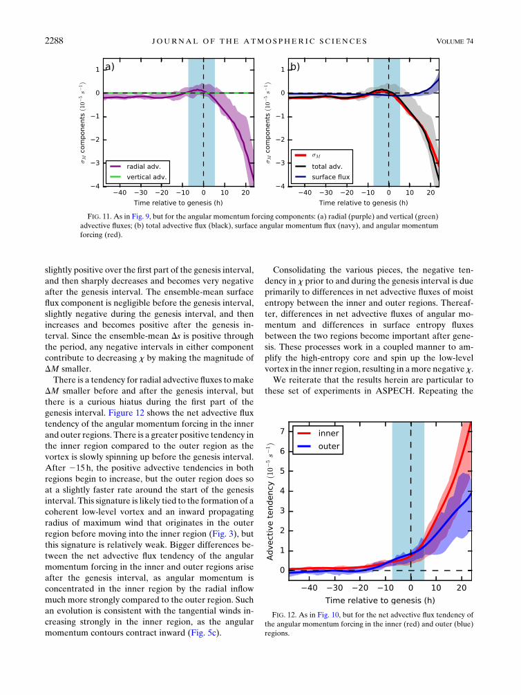
slightly positive over the first part of the genesis interval,

and then sharply decreases and becomes very negative

after the genesis interval. The ensemble-mean surface

flux component is negligible before the genesis interval,

slightly negative during the genesis interval, and then

increases and becomes positive after the genesis in-

terval. Since the ensemble-mean Ds is positive through

the period, any negative intervals in either component

contribute to decreasing x by making the magnitude of

DM smaller.

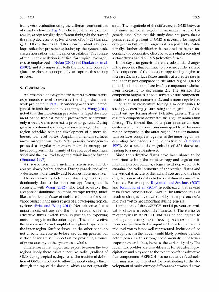
There is a tendency for radial advective fluxes tomake

DM smaller before and after the genesis interval, but

there is a curious hiatus during the first part of the

genesis interval. Figure 12 shows the net advective flux

tendency of the angular momentum forcing in the inner

and outer regions. There is a greater positive tendency in

the inner region compared to the outer region as the

vortex is slowly spinning up before the genesis interval.

After 215h, the positive advective tendencies in both

regions begin to increase, but the outer region does so

at a slightly faster rate around the start of the genesis

interval. This signature is likely tied to the formation of a

coherent low-level vortex and an inward propagating

radius of maximum wind that originates in the outer

region before moving into the inner region (Fig. 3), but

this signature is relatively weak. Bigger differences be-

tween the net advective flux tendency of the angular

momentum forcing in the inner and outer regions arise

after the genesis interval, as angular momentum is

concentrated in the inner region by the radial inflow

much more strongly compared to the outer region. Such

an evolution is consistent with the tangential winds in-

creasing strongly in the inner region, as the angular

momentum contours contract inward (Fig. 5c).

Consolidating the various pieces, the negative ten-

dency in x prior to and during the genesis interval is due

primarily to differences in net advective fluxes of moist

entropy between the inner and outer regions. Thereaf-

ter, differences in net advective fluxes of angular mo-

mentum and differences in surface entropy fluxes

between the two regions become important after gene-

sis. These processes work in a coupled manner to am-

plify the high-entropy core and spin up the low-level

vortex in the inner region, resulting in amore negative x.

We reiterate that the results herein are particular to

these set of experiments in ASPECH. Repeating the

FIG. 11. As in Fig. 9, but for the angular momentum forcing components: (a) radial (purple) and vertical (green)

advective fluxes; (b) total advective flux (black), surface angular momentum flux (navy), and angular momentum

forcing (red).

FIG. 12. As in Fig. 10, but for the net advective flux tendency of

the angular momentum forcing in the inner (red) and outer (blue)

regions.

2288 JOURNAL OF THE ATMOSPHER IC SC IENCES VOLUME 74

framework evaluation using the different combinations

of ri and ro shown in Fig. 6 produces qualitatively similar

results, except for slightly different timings in the start of

the sharp decrease of x. For choices of ri . 225 km and

ro . 300 km, the results differ more substantially, per-

haps reflecting processes spinning up the system-scale

circulation rather than the inner circulation. The spinup

of the inner circulation is critical for tropical cyclogen-

esis, as emphasized inNolan (2007) andDunkerton et al.

(2009), and it is important both the inner and outer re-

gions are chosen appropriately to capture this spinup

process.

5. Conclusions

An ensemble of axisymmetric tropical cyclone model

experiments is used to evaluate the diagnostic frame-

work presented in Part I. Moistening occurs well before

genesis in both the inner and outer regions.Wang (2014)

noted that this moistening precedes the rapid develop-

ment of the tropical cyclone protovortex. Meanwhile,

only a weak warm core exists prior to genesis. During

genesis, continued warming and moistening of the inner

region coincides with the development of a more co-

herent, low-level vortex. Angular momentum surfaces

move inward at low levels. After genesis, frontogenesis

proceeds as angular momentum and moist entropy sur-

faces compress in the vicinity of the radius of maximum

wind, and the low-level tangential winds increase further

(Emanuel 1997).

As viewed from the x metric, x is near zero and de-

creases slowly before genesis. During genesis and after,

x decreases more rapidly and becomes more negative.

The decrease in x before and during genesis is pre-

dominately due to the moist entropy forcing and is

consistent with Wang (2012). The total advective flux

component dominates the moist entropy forcing, much

like the horizontal fluxes ofmoisture dominate the water

vapor budget in the inner region of a developing tropical

cyclone (Fritz and Wang 2014). Net advective fluxes

import moist entropy into the inner region, while net

advective fluxes switch from importing to exporting

moist entropy from the outer region. The net advective

fluxes increase Ds and amplify the high-entropy core in

the inner region. Surface fluxes, on the other hand, do

not directly increase Ds before and during genesis, but

surface fluxes are still important for providing a source

of moist entropy to the system as a whole.

Differences in net import and export between the two

regions imply there exists a positive radial gradient of

GMS during tropical cyclogenesis. The traditional defini-

tion of GMS is modified to allow for moist entropy fluxes

through the top of the domain, which are not generally

small. The magnitude of the difference in GMS between

the inner and outer regions is maximized around the

genesis time. Note that this study does not prove that a

positive radial gradient of GMS is necessary for tropical

cyclogenesis but, rather, suggests it is a possibility. Addi-

tionally, further clarification is required to better un-

derstand the cooperative effect between radial gradients of

surface fluxes and the GMS (advective fluxes).

In the day after genesis, there are substantial changes

in the processes that continue to decrease x. The surface

flux component of the moist entropy forcing begins to

increase Ds, as surface fluxes amplify at a greater rate in

the inner region compared to the outer region. On the

other hand, the total advective flux component switches

from increasing to decreasing Ds. The surface flux

component outpaces the total advective flux component,

resulting in a net increase in Ds and a more negative x.

The angular momentum forcing also contributes to

strongly decreasing x, surpassing the magnitude of the

moist entropy forcing about 15 h after genesis. The ra-

dial flux component dominates the angular momentum

forcing. The inward flux of angular momentum con-

centrates angular momentum more quickly in the inner

region compared to the outer region. Angular momen-

tum surfaces compress together in the inner region, ac-

celerating frontogenesis and intensification (Emanuel

1997). As a result, the magnitude of DM decreases,

leading to a more negative x.

Since the advective fluxes have been shown to be

important to both the moist entropy and angular mo-

mentum flux components, a logical next step would be to

examine the radial structure of the vertical fluxes and

the vertical structure of the radial fluxes around the time

of genesis in relationship to the evolution of convective

features. For example, Raymond and Sessions (2007)

and Raymond et al. (2014) hypothesized that inward

mass fluxes concentrated lower in the atmosphere as a

result of changes in vertical stability in the presence of a

midlevel vortex are important during genesis.

Limitations of the ASPECH model prevent an eval-

uation of some aspects of the framework. There is no ice

microphysics in ASPECH, and thus no cooling due to

melting and heating due to freezing. As a result, strati-

form precipitation that is important to the formation of a

midlevel vortex is not well represented. Inclusion of ice

microphysics in the model would likely produce periods

before genesis with a stronger cold anomaly in the lower

troposphere and, thus, increase the variability of x. The

radial flux profiles are also different for stratiform pre-

cipitation andmay change the evolution of the advective

flux components. ASPECH has no radiative feedbacks

that may also be important for contributing to the de-

velopment ofmoist entropy differences between the two

JULY 2017 TANG 2289

regions. Radiative feedbacks have been shown to be

important for the aggregation of convection in an ide-

alized model (Wing and Emanuel 2014) and may aid

tropical cyclogenesis as well (Wing et al. 2016). Another

limitation is the representation of genesis with a 2D

model with rings of convection versus a 3D model with

more realistic convection. It would be interesting to see

if the results from this study hold for an ensemble of 3D

simulations and is the subject of future work. Last, it

would be interesting to repeat these experiments for a

mix of cases that do undergo genesis and fail to undergo

genesis to determine which conditions are necessary for

genesis or sufficient to prohibit genesis.

While observations are not of high-enough time and

spatial resolution to fully take advantage of the frame-

work, composites of dropsondes and/or remotely sensed

variables in developing disturbances may be used to

calculate bulk differences of moist entropy and angular

momentum across meso-beta-scale regions separated by

the emerging radius of maximum wind in order to assess

whether there is a similar behavior of x around the time

of genesis. Full-physics 3D model simulations or en-

sembles could then be used to assess the processes

controlling x for real-world cases. A reexamination of

cases from past field campaigns using this framework

could be a useful starting point.

Acknowledgments. Will Komaromi and two anony-

mous reviewers helped improve the manuscript. The

University at Albany Faculty Research Award Program

Award 64949 supported a portion of this work.

REFERENCES

American Meteorological Society, 2012: Tropical depression.

Glossary of Meteorology. [Available online at http://glossary.

ametsoc.org/wiki/Tropical_depression.]

Bister, M., and K. A. Emanuel, 1997: The genesis of Hurricane

Guillermo: TEXMEX analyses and a modeling study.Mon.Wea.

Rev., 125, 2662–2682, doi:10.1175/1520-0493(1997)125,2662:

TGOHGT.2.0.CO;2.

Black, P. G., and Coauthors, 2007: Air–sea exchange in hurricanes:

Synthesis of observations from the Coupled Boundary Layer

Air–Sea Transfer experiment. Bull. Amer. Meteor. Soc., 88,

357–374, doi:10.1175/BAMS-88-3-357.

Bryan, G. H., and R. Rotunno, 2009: The maximum intensity of

tropical cyclones in axisymmetric numerical model simulations.

Mon. Wea. Rev., 137, 1770–1789, doi:10.1175/2008MWR2709.1.

Cecelski, S. F., and D.-L. Zhang, 2013: Genesis of Hurricane Julia

(2010) within anAfrican easterly wave: Low-level vortices and

upper-level warming. J. Atmos. Sci., 70, 3799–3817,

doi:10.1175/JAS-D-13-043.1.

Davis, C. A., and D. A. Ahijevych, 2012: Mesoscale structural

evolution of three tropical weather systems observed during

PREDICT. J. Atmos. Sci., 69, 1284–1305, doi:10.1175/

JAS-D-11-0225.1.

Dolling, K., and G. M. Barnes, 2012: Warm-core formation in

Tropical StormHumberto (2001).Mon. Wea. Rev., 140, 1177–

1190, doi:10.1175/MWR-D-11-00183.1.

Dunion, J. P., 2011: Rewriting the climatology of the tropical North

Atlantic and Caribbean Sea atmosphere. J. Climate, 24, 893–

908, doi:10.1175/2010JCLI3496.1.

Dunkerton, T. J., M. T. Montgomery, and Z. Wang, 2009: Tropical

cyclogenesis in a tropical wave critical layer: Easterly waves.

Atmos. Chem. Phys., 9, 5587–5646, doi:10.5194/acp-9-5587-2009.

Emanuel, K. A., 1997: Some aspects of hurricane inner-core dy-

namics and energetics. J. Atmos. Sci., 54, 1014–1026, doi:10.1175/

1520-0469(1997)054,1014:SAOHIC.2.0.CO;2.

Fritz, C., and Z. Wang, 2014: Water vapor budget in a developing

tropical cyclone and its implication for tropical cyclone forma-

tion. J. Atmos. Sci., 71, 4321–4332, doi:10.1175/JAS-D-13-0378.1.

Grabowski, W. W., 2003: Impact of ice microphysics on multiscale

organization of tropical convection in two-dimensional cloud-

resolving simulations. Quart. J. Roy. Meteor. Soc., 129, 67–81,

doi:10.1256/qj.02.110.

Hartmann, D. L., J. R. Holton, and Q. Fu, 2001: The heat balance

of the tropical tropopause, cirrus, and stratospheric de-

hydration. Geophys. Res. Lett., 28, 1969–1972, doi:10.1029/

2000GL012833.

Kerns, B. W., and S. S. Chen, 2015: Subsidence warming as an

underappreciated ingredient in tropical cyclogenesis. Part I:

Aircraft observations. J. Atmos. Sci., 72, 4237–4260,

doi:10.1175/JAS-D-14-0366.1.

Kessler, E., 1969: On the Distribution and Continuity of Water

Substance in Atmospheric Circulations. Meteor. Monogr.,

No. 32, Amer. Meteor. Soc., 88 pp.

Kilroy, G., R. K. Smith, and M. T. Montgomery, 2017: A unified

view of tropical cyclogenesis and intensification.Quart. J. Roy.

Meteor. Soc., 143, 450–462, doi:10.1002/qj.2934.

Knaff, J. A., C. R. Sampson, P. J. Fitzpatrick, Y. Jin, and C.M. Hill,

2011: Simple diagnosis of tropical cyclone structure via pres-

sure gradients. Wea. Forecasting, 26, 1020–1031, doi:10.1175/

WAF-D-11-00013.1.

Komaromi, W. A., 2013: An investigation of composite dropsonde

profiles for developing and nondeveloping tropical waves

during the 2010 PREDICT field campaign. J. Atmos. Sci., 70,

542–558, doi:10.1175/JAS-D-12-052.1.

Lussier, L. L., III, M. T. Montgomery, and M. M. Bell, 2014: The

genesis of Typhoon Nuri as observed during the Tropical

Cyclone Structure 2008 (TCS-08) field experiment—Part 3:

Dynamics of low-level spin-up during the genesis. Atmos.

Chem. Phys., 14, 8795–8812, doi:10.5194/acp-14-8795-2014.

Montgomery, M. T., and Coauthors, 2012: The Pre-Depression

Investigation of Cloud-Systems in the Tropics (PREDICT)

experiment: Scientific basis, new analysis tools, and some first

results. Bull. Amer. Meteor. Soc., 93, 153–172, doi:10.1175/

BAMS-D-11-00046.1.

Nguyen, L. T., J. Molinari, and D. Thomas, 2014: Evaluation of

tropical cyclone center identification methods in numerical

models. Mon. Wea. Rev., 142, 4326–4339, doi:10.1175/

MWR-D-14-00044.1.

Nolan, D. S., 2007: What is the trigger for tropical cyclogenesis?

Aust. Meteor. Mag., 56, 241–266.Raymond, D. J., and S. L. Sessions, 2007: Evolution of convection

during tropical cyclogenesis. Geophys. Res. Lett., 34, L06811,

doi:10.1029/2006GL028607.

——, C. López-Carrillo, and L. L. Cavazos, 1998: Case-studies of

developing east Pacific easterly waves. Quart. J. Roy. Meteor.

Soc., 124, 2005–2034, doi:10.1002/qj.49712455011.

2290 JOURNAL OF THE ATMOSPHER IC SC IENCES VOLUME 74

——, S. L. Sessions, and �Z. Fuchs, 2007: A theory for the spinup of

tropical depressions. Quart. J. Roy. Meteor. Soc., 133, 1743–

1754, doi:10.1002/qj.125.

——, ——, and C. López-Carrillo, 2011: Thermodynamics of

tropical cyclogenesis in the northwest Pacific. J. Geophys. Res.,

116, D18101, doi:10.1029/2011JD015624.

——, S. Gjorgjievska, S. L. Sessions, and �Z. Fuchs, 2014: Tropical

cyclogenesis and mid-level vorticity. Aust. Meteor. Oceanogr.

J., 64, 11–25, doi:10.22499/2.6401.003.

Smith, R. K., 2006: Accurate determination of a balanced axi-

symmetric vortex in a compressible atmosphere. Tellus, 58A,

98–103, doi:10.1111/j.1600-0870.2006.00149.x.

Stern, D. P., and D. S. Nolan, 2012: On the height of the warm core

in tropical cyclones. J. Atmos. Sci., 69, 1657–1680, doi:10.1175/

JAS-D-11-010.1.

Tang, B. H., 2017: Coupled dynamic–thermodynamic forcings

during tropical cyclogenesis. Part I: Diagnostic framework.

J. Atmos. Sci., 74, 2269–2278, doi:10.1175/JAS-D-17-0048.1.

——, and K. Emanuel, 2012: Sensitivity of tropical cyclone in-

tensity to ventilation in an axisymmetric model. J. Atmos. Sci.,

69, 2394–2413, doi:10.1175/JAS-D-11-0232.1.

——, R. Rios-Berrios, J. J. Alland, J. D. Berman, and K. L.

Corbosiero, 2016: Sensitivity of axisymmetric tropical cyclone

spinup time to dry air aloft. J. Atmos. Sci., 73, 4269–4287,

doi:10.1175/JAS-D-16-0068.1.

Van Sang, N., R. K. Smith, andM. T. Montgomery, 2008: Tropical-

cyclone intensification and predictability in three dimensions.

Quart. J. Roy. Meteor. Soc., 134, 563–582, doi:10.1002/qj.235.

Wang, Z., 2012: Thermodynamic aspects of tropical cyclone

formation. J. Atmos. Sci., 69, 2433–2451, doi:10.1175/

JAS-D-11-0298.1.

——, 2014: Role of cumulus congestus in tropical cyclone forma-

tion in a high-resolution numerical model simulation.

J. Atmos. Sci., 71, 1681–1700, doi:10.1175/JAS-D-13-0257.1.

——, M. T. Montgomery, and T. J. Dunkerton, 2010: Genesis of

pre–Hurricane Felix (2007). Part I: The role of the easterly

wave critical layer. J. Atmos. Sci., 67, 1711–1729, doi:10.1175/

2009JAS3420.1.

Wing, A. A., and K. A. Emanuel, 2014: Physical mechanisms

controlling self-aggregation of convection in idealized nu-

merical modeling simulations. J. Adv. Model. Earth Syst., 6,

59–74, doi:10.1002/2013MS000269.

——, S. J. Camargo, and A. H. Sobel, 2016: Role of radiative–

convective feedbacks in spontaneous tropical cyclogenesis in

idealized numerical simulations. J. Atmos. Sci., 73, 2633–2642,

doi:10.1175/JAS-D-15-0380.1.

Zawislak, J., and E. J. Zipser, 2014: Analysis of the thermodynamic

properties of developing and nondeveloping tropical distur-

bances using a comprehensive dropsonde dataset. Mon. Wea.

Rev., 142, 1250–1264, doi:10.1175/MWR-D-13-00253.1.

Zhang, D.-L., and L. Zhu, 2012: Roles of upper-level processes in

tropical cyclogenesis. Geophys. Res. Lett., 39, L17804,

doi:10.1029/2012GL053140.

Zhang, F., and J. A. Sippel, 2009: Effects of moist convection on

hurricane predictability. J. Atmos. Sci., 66, 1944–1961,

doi:10.1175/2009JAS2824.1.

JULY 2017 TANG 2291