
COUPLED DYNAMICS ANALYSIS OF WIND ENERGY SYSTEMS
86
NASA CR-135152 Paragon 1014-11 COUPLED DYNAMICS ANALYSIS OF WIND ENERGY SYSTEMS JOHN A. HOFFMAN Paragon Pacific Incorporated El Segundo, California (NAS-A-CR-135152) COUPLED DYNAMICS ANALYSIS OF WIND ENERGY SYSTEMS Final Report (Paragon Pacific, Inc., El Segundo, Calif.) 86 p HC A05/MF A01 CSCL 10A prepared for G3/4 N!7-20558 Unclas 21740 NATIONAL AERONAUTICS AND SPACE ADMINISTRATION Lewis Research Center Cleveland, Ohio February 1977 Contract NAS 3-19767 REPRODUCED BY NATIONAL TECHNICAL -INFORMATION 'SERVICE * U.S. DEPARTMENT OF COMMERCE SPRINGFIELD, VA_ 22161 https://ntrs.nasa.gov/search.jsp?R=19770013614 2018-04-08T06:11:45+00:00Z
-
Upload
nguyenkhue -
Category
Documents
-
view
223 -
download
0
Transcript of COUPLED DYNAMICS ANALYSIS OF WIND ENERGY SYSTEMS
NASA CR-135152
Paragon 1014-11
COUPLED DYNAMICS ANALYSIS
OF WIND ENERGY SYSTEMS
JOHN A HOFFMAN
Paragon Pacific Incorporated
El Segundo California
(NAS-A-CR-135152) COUPLED DYNAMICS ANALYSIS OF WIND ENERGY SYSTEMS Final Report (Paragon Pacific Inc El Segundo Calif) 86 p HC A05MF A01 CSCL 10A
prepared for
G34
N7-20558
Unclas 21740
NATIONAL AERONAUTICS AND SPACE ADMINISTRATION
Lewis Research Center
Cleveland Ohio
February 1977
Contract NAS 3-19767
REPRODUCED BY NATIONAL TECHNICAL
-INFORMATION SERVICE US DEPARTMENT OF COMMERCE SPRINGFIELD VA_ 22161
httpsntrsnasagovsearchjspR=19770013614 2018-04-08T061145+0000Z
1 Report No 2 Gorrane Accinwn No 3 Reclipets Cast g No
4 Title and Subtitle S Report Date January 1977
COUPLED DgRAHECS 6 Performing Organization Code
7 Aithor(sl S Performing Organization Report No
John A Hofftan Pp-oiI4-1n 10 Work Unit No
9 Performing Organization Name and Address
Paragon Pacific Inc 11 Contract or Grant No 1601 E El Segundo Blvd El Segundo California 90245 NAS3-19767
13 Type of Report and Period Covered 12 Sponsoring Agency Name and Address Contractor Final Report
National Aeronautics and Space Administration 14 Sponsoring Agency Code Lewis Research Center Cleveland Ohio
15 Supplementary Notes
16 Abstract
A qualitative description of all key elements of a complete wind energy system computer analysis code is presented The analysis system addresses the coupled dynamics characteristics of wind energy systems including the interactions of the rotor tower nacelle power train control system and electrical network The coupled dynamics are analyzed in both the frequency and time domains to provide the basic motions and loads data required for design performance verification and operations analysis activities
Elements of the coupled analysis code were used to design and analyze candidate rotor articulation concepts for the NASAERDA Mod 0 Wind Turbine System Fundamental results and conclusions derived from these studies are presented
The analysis results show that the teetering rotor develops apprximateyhalftbeblade flap bending loads produced by a rigidly mounted hingeless rotor using identical blades Edgewise blade loads are approximately equal in the two systems
Flexibilities in the Mod 0 yaw drive tower nacelle and bearing mounts appear to be allowing the hingeless Mod 0 rotor to teeter to a substantial degree Hence the measured 2dod 0 load levels are midway between calculated loads for the bingeless and teetering designs
Hingeless rotors with blade frequencies substnatially below those of the current Mcd 0 system develop lower flap bending loads at the expense of significantly higher edgewise bending loads Such systems also require more bladetower clearance to accommodate larger rotor coning excurshysions over the wind turbine system operational envelope
17 Key Words (Suggested by Author(s)) 18 Distribution Statement
Wind Energy Machines Unclassified - limited
Windmills Wind-Power Generators
Windmill Dynamics Wind Turbine Dynamics
19 Sectrity Clasif (of this report) 20 Security Classif (of this page)
Unclassified i Unclassifiedt
For sale by the National Technical Information Service Springfield Virginia 22161
NASA-C-l68 (Rev 10-75)
ORIGINL PAGE IS OF POO QUALM
FOREWORD
The work documented by this report was performed under Contract NAS 3-19767 issued by the NASA Lewis Research Center Cleveland Ohio 44135 The contract work was performed by Paragon Pacific Inc El Segundo California 90245 under the direction of Mr David C Janetzke of NASA Lewis Research Center
The author wishes to express sincere appreciation for the efforts of Mr Janetzke in his support of the contractual work which included guidance in designing and confirming the analytic computer codes and the assembly of fundamental input data for these analysis methods as applicable to the NASAERDA Mod 0 Wind Turbine System
iii Preceding page blank
TABLE OF CONTENTS
Page
FOREWORD iii
SUMMARY 1
INTRODUCTION 2
Evolution of the Wind Energy System Analysis Codes 2
Fundamental Objectives for the Coupled Dynamics Analysis Code 3
Design and Analysis of Candidate Mod-O Rotor Articulation Concepts 5
Organization of the Remaining Sections of this Report 5
OVERALL SYSTEM DESCRIPTION - WIND ENERGY SYSTEM COUPLED DYNAMICS ANALYSIS CODE 6
Overall System Arrangement 6
Subcode Data Interfaces 7
Sequence of Events - Coupled System Analysis 7
Fundamental Assumptions Incorporated in the Analysis 9
Alternative Analysis Methods 10
COMPONENT MODEL DESCRIPTIONS 12
Datain 12
Mostab-M 12
Rolim 14
The Coupled System Linear Analysis 14
DESIGN AND ANALYSIS OF CANDIDATE MOD 0 HUB ARTICULATION CONCEPTS 26
The Teetering System 26
The Elastic Interface Devices 27
General Conclusions - Articulation Devices 29
DISCUSSION OF RESULTS 29
CONCLUSIONS AND RECOMMENDATIONS FOR FURTHER RESEARCH 30
Verification of MOSTAS 30
Improved Accuracy 30
v - rceh page blank
Select Nonlinearities 31
Utility Items 31
REFERENCES 32
TABLES
I History of MOSTABROLIM Systems 33
II Data Interfaces by Subcode Wind Energy System Coupled Dynamics Analysis 34
III Methods of Dynamic Analysis -- Rotor Systems 4o
IV Vectors for Wind Turbine Coupled System 41
V Operators for Wind Turbine Coupled System 43
VI Vector Lengths for Wind Turbine Coupled System 47
VII Teetering Hub Design Concepts - Weights and Other Design Data 48
VIII Blade Root Flexures - Summary 49
FIGURES
1 Coupled Dynamics Analysis (MOSTAS) - Global Arrangements 50
2 Time and Frequency Domain Analysis Methods 51
3 Basic MOSTABROLIM Analysis Procedures 52
4 Essential Elements of MOSTAB Math Models 53
5 MOSTAB Executive Logical Procedure 54
6 Fundamentals of Rotor Analysis 55
7 Aeroelastic Blade Analysis 56
8 Gimbal Analysis 57
9 Advanced Shadow Model 58
10 MOSTAB Outputs 59
11 Steps in ROLIM Process 6o
12 The Rotor Linear Modelling Program ROLIM 61
13 Example ROLIM Printouts 62
14 Tower Math Model 63
15 Sample Control System Model 64
16 Power Train Dynamic Math Model 65
17 Wind Turbine System Block Diagram 66
18 Long Yoke Teetering Design 67
vi
6819 Short Yoke Teetering Concept
6920 Linkage Teetering Concept
21 Root Out-Of-Plane Moment 70
22 Root In-Plane Moment 71
7223 Blade Tip Deflection
24 Blade Moment Reduction Expected from Teetering as a Stiffness 73Function of Present Hub Support
74Elastic Interface Flexure A 25
26 Elastic Interface Flexure B 75
27 Elastic Interface Flexure C I 76
28 Elastic Interface Flexure D 77
29 Root Out-Of-Plane Bending Moment 78
30 Root In-Plane Bending Moment 79 8o31 Blade Tip Deflection
vii
COUPLED DYNAMICS ANALYSIS
OF WIND ENERGY SYSTEMS
John A Hoffman
Paragon Pacific Inc
SUMMARY
A qualitative description of all key elements of a complete wind energy system computer analysis code is presented The analysis system addresses the coupled dynamics characteristics of wind energy systems including the interactions of the rotor tower nacelle power train control system and electrical network The coupled dynamics are analyzed in both the frequency and time domains to provide the basic motions and loads data required for design performance verification and operations analysis activities
Elements of the coupled analysis code were used to design and analyze candidate rotor articulation concepts for the NASAERDA Mod 0 Wind Turbine System Fundamental results and conclusions derived from these studies are presented
INTRODUCTION
This report presents a comprehensive description of a complete wind energy system digital computer analysis code Also presented are fundamental analysis results pr-oduced by the coupled dynamitcs programs as applicable to the NASA Mod 0 Wind Turbine at Sandusky Ohio The analysis results address the baseline Mod 0 system and variations from this baseline design associated with various rotor articulation concepts
The fundamental emphasis of this report is directed toward a complete definition of the wind turbine system computer analysis focusing on the assumptions and procedures of the methods and the types of problems the system can solve The detailed equations and logic coded in the analysis programs and the users information required to effectively use these codes being very voluminous are provided in References 1 through 3 inclusive
Evolution of the Wind Energy System Analysis Codes
The wind energy system coupled dynamics analysis program was developed using existing methods and codes synthesized originally for application to rotorcraft The MOdular STABility Derivative Program (MOSTAB) series and the ROtor LInear Modelling Code (ROLIM) represent the contributions of these original analysis systems MOSTAB and ROLIM were developed over a period of many years and found financial support from a number of sources Table I presents a brief history of the developments of these baseline codes for general reference
An early version of MOSTAB MOSTAB-C (M-C) was first converted for application to wind energy system analysis This program MOSTAB-WT has been used extensively for wind turbine rotor performance and preliminary loads analysis The analysis methods and procedures incorporated in MOSTAB-WT have been documented in Reference 4 References 5 and 6 present results derived in part using MOSTAB-WT as these apply to various phases of wind energy system analysis
Although MOSTAB-WT provided much useful information about wind turbine performance and dynamics it was recognized that much more advanced analysis methods would eventually be required for comprehensive treatment of these complex dynamic systems MOSTAB-WT includes the dynamics of the first flapshyping mode of the blade - considered adequate for most performance examinations and for preliminary motions and loads analysis The rotorcraft technology suggested the extreme importance of higher frequency blade dynamics however as these affect dynamic loads overall system aeromechanical stability and dynamic response performance Additionally MOSTAB-WT assumed the fixed shaft environment wherein the rotor shaft centerline is presumed fixed in space and that the rotational speed of the shaft is maintained perfectly constant Test data taken from the MOD 0 Wind Turbine and past experience in the rotoreraft technology suggested that the fixed shaft assumption would mask critical dynamic phenomena that occur through couplings among rotor blade support system power train and control system degrees of freedom
2
The early recognition of MOSTAB-WT limitations for comprehensive wind turbine dynamics analysis instigated the contractual work defined herein which has provided a complete series of coupled dynamics analysis codes applicable specifically to wind energy systems This advanced system started with the MOSTAB-HFA version (-HFA denoting High Frequency Analysis) MOSTAB-HFA is a rotorcraft analysis code that includes high frequency rotor blade degrees of freedom Additionally the coupled system analysis includesthe Rotor LInear Modelling Program (ROLIM) as a key element ROLIM uses the completenonlinear rotor models in MOSTAB-HFW (-HFW standing for the high frequency wind turbine conversion of MOSTAB-HFA) to synthesize a rigorous linear rotor model in periodic coefficients The ROLIM model is then combined with linear models for other key system components to produce the overall coupled system model required for advanced dynamic analysis of wind energy systems Th6 coupling code has been given the name WIND energy Linear Analysis Software System (WINDLASS) The complete analysis system has been named MOSTAS an acronym derived from MOSTAB and WINDLASS
Fundamental Objectives for the Coupled Dynamics Analysis Code
The basic objectives of the coupled analysis can be grouped essentially into three categories stability loads and performance
Stability refers to the tendency of the various degrees of freedom of a system-to seek a steady-state and bounded excitation once set in arbitrary motion If a system is unstable one or more system degrees of freedom will diverge without bound until either nonlinearities intervene to limit the motion or (usually catastrophic) failure of system elements involved in the motion occurs The rotorcraft technology has many kinds of aeromechanicalcontrol system instabilities that have been well publicized including ground resonance flap-lag instability classical blade flutter (flap-torsion) and variousshyinstabilities associated with control system interactions Many obvious similarities between rotorcraft and wind turbine systems can be cited These include the large aeroelasticrotor mounted on flexible supports with relatively tight-looped control system elements Hence one might strongly suspect that wind energy systems possess an affinity for aeromechanical and control system interactive instabilities In fact the wind turbine might tend to be even more prone to regions of instability in some cases because of the widely varying operating conditions involved An example of this is rotor speed which is tightly bounded to within a small variation from a nominal speed in the case of rotorcraft in flight while the wind turbine may operate over a relatively large band of speeds
Because of the stability considerations addressed above stability assessment of the coupled wind energy system dynamics represents a key requirement on the comprehensive analysis code
At the time of this writing the ROLIM system and its associated documentashytion (Reference 2) are proprietary with distribution limited to governmental agencies only
3
Loads and associated motions of the various system degrees of freedom have a major impact on system component design Test data gleaned from experimental operation of theMod 0 Wind Turbine has shown that blade loads for example can be significantly influenced by the dynamic variations of shaft position and rotor speed This conclusion would also be indicated from past rotorcraft experience Thusthe assessment of critical component dynamic loads is seen to depend on the coupled interactions among the various components of the wind energy system Tower and nacelle dynamic characteristics will allow the shaft to move in space as the rotor turns and develops time-varying blade shank loads Flexibilities in the power train provide for time-varying rotor speed as dynamically varying shaft torques produced by the rotor excite the power train elements It is likely that loops in the wind turbine control system responding to the time-varying actions of the rotor power train and supports may also participate in the coupled dynamics in a significant manner
From these considerations one places an important requirement on the coupled analysis to predict loads and motions associated with key dynamic elements of the wind energy system including the critical interactions of its various components
Performance is often thought simply to be the average power produced by the wind energy system in a given environment in a dynamic context however the term performance receives a broader interpretation When the wind turbine operates in its highly asymmetrical environment which includes excitations from the tower shadow wind shear and oblique wind approach velocities the coupled system components can respond to produce dynamically varying power output levels Hence the dynamic performance of the system refers to its ability to produce power of usable quality If the power is delivered as alternating current (AC) that is to be applied to an existing utility network with an established frequency and phase angle the wind energy system must be precisely controlled to deliver the AC power at acceptable frequency phase angle and purity (from spurious constituents) to be usable and efficiently consumable The coupled dynamic performance of all elements of the wind energy system and specifically the rotor power train electrical equipment and control system must therefore be carefully considered
In the context addressed above dynamic performance assessment becomes a critical requirement on the coupled analysis code
Other types of dynamic analysis results in addition to those addressed above can be gleaned from the analysis program addressed by this report some of these results of course may require some program refinement while others are natural components of the existing program output The specific types of analyses that can be performed by the code and the associated limiting assumptions are addressed in the remaining sections of this report The current analysis system has been developed to achieve the key goals listed above however and these are to be considered the major types of solutions thatcan be found on a routine basis using this advanced computer software
The tower shadow effect is the dynamic excitation of rotor blade loads and motions when the blades pass through the wake of an upwind tower
4
Design and Analysis of Candidate Mod-0 Rotor Articulation Concepts
A component of the subjectcontractual activity addressed the preliminary design and computer analysis of candidate rotor articulation arrangements for the Mod 0 Wind Turbine system Two classes of devices were considered the teetering suspension and blade-root elastic interfacing devices Both classes of devices were examined for the fundamental purpose of reducing blade loads of the mod 0 unit thereby extending the fatigue life of the blades The devices were to be bolt-on units involving minimum modification of existing Mod 0 hardware
Completed elements of the coupled dynamics software were used to analyze the candidate designs during the period when the full coupled analysis was being developed Time was of the essence The results gleaned from application of these analysis codes were used to derive the key conclusions associated with each candidate device
Reference 7 represents the detailed design and analysis documentation developed for the Mod 0 articulation concepts The key results and conclushysions are summarized in a later section of this report under the heading Design and Analysis of Candidate Mod 0 Hub Articulation Concepts
Organization of the Remaining Sections of this Report
The next section of this report presents a global description of the wind energy system analysis code The data interfaces among the several elements of the code each of which is executed separately in the complete analysis are shown The fundamental assumptions and procedures incorporated in the various executive sections of the overall system are addressed and the extent and validity of the results produced by each section are identified Alternative analysis procedures which could be implemented are also addressed and the fundamental reasons why the approach taken for the coupled analysis was selected from the candidates are given
A description of each element of the coupled analysis code is then presented Basic logical procedures incorporated in each segment are addressed Assumpshytions and methods incorporated in the various analyses are addressed in more detail than presented previously
The next section presents a summary of the results and conclusions derived during the design and analysis of the Mod 0 rotor articulation concepts
Finally recommendations for further research which address practical extension and refinement of the current wind energy system analysis software are extended in the remaining section of the report
5
OVERALL SYSTEM DESCRIPTION - WIND ENERGY SYSTEM COUPLED DYNAMICS ANALYSIS CODE
This section sunnarizes the operation of the total analysis system concentrating on-the data interfaces and analysis results from each subsystem A discussion of candidate analysis procedures is also presented identifying the basic reasons for taking the selected approach
Overall System Arrangement
Figure 1 is a block diagram depicting the overall system arrangement currently incorporated in the coupled dynamics analysis software Each rectangular block represents an independent executive computer code With the input data provided as indicated each of these programs can be executed to completion producing essential output information in each case The hexagonal figures indicate data read from cards by each executive subsystem and the curved figures summarize the information printed by each subcode Other data interfaces indicated by lines are tape or disk files
The system has been arranged as indicated by Figure 1 for economy Since the full wind energy system analysis can be performed in a series of independent steps the steps are executed separately to minimize the required use of -computer storage Additionally when a series of analyses-is being performed suboodes need to be executed only when a change has occurred in its input data Often an entire series of analyses can be performed by serially executing only one or two of the five basic subcodes
To see the storage use features of this arrangement consider the storage requirements System DATAIN is essentially an Inputoutput (IO) function which reads the basic MOSTAB input data and verify-writes the data in a formatshyted printout Such an IO function is required only when the MOSTAB data changes an appreciable amount of storage is involved in this IO operation engaging relatively complex FORMAT statements that are not needed by any of the other subcodes Hence when the DATAIN execution is complete its presence in storage is destroyed making that storage available for use by other subshycodes
Similar explanations apply to the other subcodes in the system For example MOSTAB-HFW involves the use of considerable storage for the complex rotor blade math models including the nonlinear inertial and aerodynamic distributed loading functions radial and azimuthal numerical integration algorithms etc Once the trim condition is found by MOSTAB and the loads and motions data (the PROCES file) and the linear model (the ROLIM file) are produced the complex MOSTAB models are no longer required and can be unloaded
Executive efficiency is also enhanced by the arrangement of Figure 1 For example suppose the coupled system analysis is being used to investigate the effect of a flexible coupling stiffness in the power train A series of analyses are to be performed at various operating conditions as the stiffness
6
is varied In this case the DATAINMOSTABPROCESROLIM executions need to be made only as the wind environment and rotor speed are changed These analysis executions result eventually in a series of ROLIM math models probably stored permanently on tape or disk These same models can be used over and over again as the power train design is changed The linear analysis would be re-executed for the series of operating conditions (on the ROLIM file) at each stiffness value Overall system stability loads and dynamic performance would be detershymined for each stiffness value by successive re-execution of a comparatively small portion of the total analysis software system
The ability to segment the analysis in a manner optimized for system component synthesis (as exemplified by the flexible coupling project described above) is a key reason for selecting this particular analysis approach taken here The trades between this approach and popular candidate methods are discussed in more detail in a subsequent section
Subcode Data Interfaces
The data interfaces summarized by Figure 1 represent the input data required for and the outputs produced by each executive subcode The data interfaces are interconnected by various media including the card reader and punch tape disk and drum files and the line printer Table II presents a summary description of these data interfaces serving to define in qualitative terms the input data requirements of each subcode and the useful data proshyduced by each module
Sequence of Events - Coupled System Analysis
The software system typically operates according to the series of-events described below in performing a complete coupled analysis This series could be implemented as one computer job with the described series of individual executions or perhaps more likely the user would inspect intermediate job steps prior to the instigation of successive computational tasks As mentioned above all subcodes will generally not require execution for a series of analyses
DATAIN execution will use the basic MOSTAB input data defined in detail in Reference 3 and qualitatively by Table II This step is low risk and would fail only if input data errors are encountered or if the input data prepared by the user exceeds prescribed storage limitations The DATAIN results will be printed and a tape or disk file will be created for access by the next executive subcode MOSTAB-BEW
MOSTAB-FW upon reading the DATAIN file attempts to find a trim solution Trim occurs when compatible sits of rotor loads and wake variables have been determined and when a blade-motion history (as a function of rotor azimuthal position) has been determined which is periodic If a gimballed rotor analysis is being performed (eg teetering or floating hub rotor articulation arrangements) the gimbal error function described in
7
Reference 2 must also be driven to zero within acceptable limits This analysis step represents the most hazard to the success of an overall system analysis due to potential failure of the trim-search process The trim search can fail if input data estimates are so far from the true case as to drive the rotor airfoils into areas of extreme nonlinearity (stall) If this happens_a successful trim search can almost always be achieved by rerunning the case with improved estimates
MOSTAB-HFW prints the key results of the trim-search process and also generates two disk or tape data files as indicated by Figure 1 These files are processed by the successive executions of subcodes PROCES and ROLIM
PROCES is a relatively simple subcode which reads the PROCES data file produced by MOSTAB-HFW and prints the data as a function of blade azimuth and radius Only four cards are read by PROCES three of which are arbitrary title cards and one of which is a data file unit number and executive option index card This submodule presents essentially zero risk to successful completion unless there are errors in the input data - no indeterminable outshycome events (eg iterations) are involved
PROOES performs a harmonic analysis of the blade loads for convenience This relatively small and simple subcode will probably be modified from time to time by the user to perform various functions on the loads and motion data For example a relatively simple algorithm can be devised to scan the data and select maximum and minimum loads (for a full azimuthal sweep) at selected radial stations of interest In this way the relatively large PROCES data file can be reduced to a small set of relevant numbers say for input to cumulative fatigue damage analyses
ROLIM performs a series of complex data processes using standard matrix procedures The single blade linear math model produced by MOSTAB-HFW (ROLIX) for example is expanded to represent all blades in the rotor The blades are aerodynamically coupled by the linear wake models also produced by ROLIMX
Despite the relative complexity of the ROLIM processes they do not involve indeterminable-outcome events (iterations numerical integrations etc) so that the ROLIM processes will occur with minimum failure risk The usershyprepared card inputs to ROLIM are very abbreviated (five cards three of which are title cards and the rest of which involve various executive option indices)
The system user will probably execute a series of MOSTAB-HFWPROCESROLIM cases and create a ROLIM data file series representing the operation of a given wind turbine system for varying wind and rotor speeds These data series can then be used repetitively by the coupled system linear analysis subcode
The Coupled Dynamics Linear Analysis Subcode reads the ROLIM data tape and a relatively substantial amount of system physical data from cards and assembles the linear system equations This portion of the coupled system analysis involves matrix processing which derives linear math models for all system components (except the rotor) from cards and combines these with the ROLIM rotor model to yield the coupled system equations
8
I Two coupled system equation sets emerge and these are c6mbined to elimi- nate a group of removable variables to yield a single linear equation of the form
MW+BW+Kw = WvV
where w is a column of system degrees of freedom including contributions from the rotor tower power train and control system v is a column of externally defined variables and includes such items as control system rotor speed inputcommands The upper case notation in the equation represents constant matrix operators
The eigenvalues of the lefthand side of the dynamic equation reflect the system stability characteristics so these are computed in the analysis The forced response of the equation is calculated by including the shaft and torqueloads generated by MOSTAB-HFW in v Recalling that the MOSTAB-HFW loads assume a fixed shaft and constant rotor speed one sees that the w response to these loads represents the result of shaft motion Superimposing the fixed shaft loads with the perturbation loads yields the full coupled system loads These computations are made in the linear analysis subcode in the time domain and output to the lihe printer
Fundamental Assumptions Incorporated in the Analysis
Each subeode depicted by Figure 1 of course contains its own basic assumptions These are partially identified in the next major section and in detail in References 1 through 3- There are a series of global assumptionshowever that one might identify as being applicable to the analysis system as a whole These are listed below
Superposition - The MOSTAB-HFW execution involves a full nonlinear set of equations that are solved for a given operating condition presuming a fixed shaft quiescent control inputs and constant rotor speed Then the coupled system analysis is performed using linear models and the linear and quiescent(MOSTAB-HFW) motions and loads-solutions are then superimposed to yield the final loads and motions results If the shaft control system or power train degrees of freedom become excited to extreme amplitudes for a particularoperating condition some nonlinear phenomena may become involved In such a case which can reasonably be considered very unusual the superimposed results may be somewhat in error As described in the final section of this report under Recomnmendations for Further Research key nonlinearities can be added to the coupled system analysis and executed in the time domain thereby removing associated errors resulting from the superposition process
It is also possible to loop back to MOSTAB-HFW with the calculated shaftshymotion results to recompute loads and motions using the full nonlinear systemmodels The looping could be recursive for convergence to an exact solution if necessary in rare instances
9
Constant Coefficients - Reference 2 describes the process in ROLIM wherein the rotor linear models are transformed to multi-blade coordinates thereby removing the once-per-rev components in the operators This process leaves the operators with substantial constant coefficient constituents and some n-per-rev constituents where n is the number of blades in the rotor This process justifies the use of the constant coefficient portion of the rotor model in- many i-nstances- -neglecting the twb- and higher-per-rev elements In some cases however (particularly in the case of rotors with two blades which lack diametrical inertial and aerodynamic symmetry) the time-varying elements should be considered Floquet analysis can be used to treat the timeshyvarying coefficients in the stability analysis (see Reference 8) and the inclusion of these elements in the time domain portion of the coupled analysis is straightforward
Alternative Analysis Methods
Many important reasons exist for selecting the analysis procedure desshycribed herein over candidate methods Some of these reasons and some signifishycant trades involved in selecting methods are discussed in this section
Perhaps the most common alternative selected in the rotorcraft field for solving the complete coupled system dynamics problem is the digital simulation procedure In the simulation math models for each system component are solved in the time domain The numerical integration of degrees of freeshydom in all components of the system occurs in a serial fashion with results lir together at the end of each numerical integration time interval Hence a time step advancement begins at an instant where all component state variables and interfacing loads are specified With the applied loads known the state variables in each system component math model are advanced over one numerical integration time interval using one of many algorithms for the advancement At the end of the interval the interfacing loads are calculated based on the newly advanced values of each component state vector and the process is then repeated serially to yield time-history records of the system response
The simulation has the advantage that nonlinearities can be included in each system component math module and the calculated results reflect these nonlinearities Additionally the full influence of the time-varying rotor phenomena is theoretically included
In spite of these significant advantages the digital simulation has many serious problems which tend to limit the practical utility of such methods A few of these problems are listed on the following page
In the rotoreraft problem the rotor nonrotating airframe propulsion system and flight control system relate analogously to the wind turbine rotor tower power train and control system elements
10
Cost - The models in the simulation must all be executed simultaneously to yield the final time-history results for a given operatingcondition Some
of these models (eg the rotor model) are very expensive to solve because of
their complexity but still musi be constantly re-executed in the simulation
even when the environmental conditions and physical parameters associated with
the model do not change This limitation raises the costs of operating the
simulation so drastically in many cases that the practical utility of the
simulation is very limited A given analysis activity can usually afford to
produce only a few results within the cost and schedular constraints involved
if a digital simulation is used
Stability Assessment - Figure 2 presents a typical time history trace
that might be produced by a digital simulation The enveloped high frequency
response characteristic is typical when aeroelastic rotor models are involved
To assess the stability of the system a relatively extensive time-history
trace must be run to determine the final response of the low frequency envelope modes Yet this costly process yields only a single result shy
whether or not the system is stable for the given parameters and operating
The relative stability (or the severity of the instability) isconditions not indicated Stability boundaries can be found using many (long) timeshy
history traces to establish only a single boundary point
Frequency domain techniques also depicted by Figure 2 show the exact
positions of the system characteristic roots revealing the stability margins
for each mode Classical control system techniques such as root-locus and
Bode methods can be used to show variations in relative stability as key
system parameters are synthesized Hence one sees thatthe frequency-domain
techniques offer significant advantages over the time-domain approach when
system stability is being evaluated These comparative advantages are sumshy
marized by Table III
Numerical Problems - Digital simulations suffer from a whole series of
numerical problems which at worst can yield the simulation inoperable or
in many cases at least can introduce significant errors in the calculated
A detailed discussion of these problems extendsbeyond the scoperesults of this report They are treated in more detail in Reference 9 In
summary these problems can be grouped as follows
1) Stability Aberration Numerical integration processes have the well
known tendency to modify the basic stability of a dynamic mode
because of the computational lags associated with numerical integrashy
tion Lightly damped modes which are common in structural systems
such as wind energy machines can be driven unstable in a digital
Often digital simulation users have to add artificialsimulation damping to such troublesome modes a process that sheds considerable
doubt on the final simulation results
Many types of numerical instabilities2)-Coupling Instabilities or stability aberrations such as those discussed above occur when
fundamentally sound system component models are coupled together
11
Because of the computational lags associated with the interfacing forcing variables a coupled assemblage of stable modules can go unstable when coupled together Simulation users sometimes interject nonphysical digital filters between troublesome modules a process which also sheds considerable doubt on the-final simulation results
Because of the manry problems associated with digital simulation the alternative procedure addressed by this report has been selected for compreshyhensive analysis of wind energy system dynamics The basic elements of the analysis method shown by Figure 1 represent those required for digital simulashytion however Hence relatively straightforward modifications could link these constituents together in the time domain to form a simulation The resulting software system would of course be subject to the drawbacks and problems listed above
COMPONENT MODEL DESCRIPTEIONS
The previous section presented a global description of the wind energy system coupled dynamics analysis showing data interfaces and describing the operation of each system subcode in abbreviated terms This section presents a more detailed discussion of the methods procedures and assumptions incorporated in each analytic subcode
Datain
Being essentially an inputoutput utility code DATAIN requires no addishytional discussion in this section
Mostab-HFW
Figure 3 presents the basic procedures incorporated in MOSTAB-HFW including the interfaces with PROCES and ROLIM addressed in the preceding section As described before MOSTAB-HFW reads the essential physical andshyoperational data specifications and then determines a trim condition using a full set of system component math models After trim is found these nonshylinear models are used by a group of subroutines managed by SR ROLIMX to produce the generic linear modelling data required by ROLIM Rotor data at trim is output for later handling by subcode PROCES as shown by Figure 3
Figure 4 presents a more detailed logical definition of the MOSTAB math models The FORCE models which include the complex aeroelastic rotor equations shown in the dashed box produce all system loads and the blade dynamic motions given the velocity acceleration and control environment Theinterference velocity components on the other hand are produced by WASH given all the system loads Hence the MOSTAB executive system iterates the FORCE and WASH models to converge to compatible load and velocity
12
sets essentially representing a simultaneous algebraic solution of the full nonlinear force andivelocity math models
-Figure 5 presents more det6il on the executive logic procedures incorporated in MOSTAB-HFW The trim-search loop makes successive estimates of the inter- ference velocity variables which are improved until convergence occurs After trix is found key results are printed the PROCES file is created and finally ROLIMX creates the linear models needed eventually by the ROLIM processor ROLIMX generates a linear model for only one rotor blade This full model which relates blade motion forcing functions and shaft loads created by the blade to all blade shaft and control degrees of freedom is created at each azimuthal station used in the blade motion numerical integrat on process ROLIX also synthesizes linear models for the wake using the WASH math models
The most complex part of the MOSTAB analysis is that used to treat aeroshyelastic rotors Figure 6 presents the coordinates and some key assumptions incorporated in MOSTAB rotor analyses The motion of the blade reference line is calculated as a function of blade azimuthal position using a modal analysis of blade dynamics (see Reference 10 for a discussion of this method of strucshytural dynamics analysis) These motions and all internal and shaft loads supported by the blade are computed by finding the distributed aerodynamic and inertial loads applied to the Blade Reference Line (BRL) at each azimuthal station used in the numerical integration process These loads of course are functions of the BRL position velocity and acceleration as a function of radius and of the shaft and control system variables (velocities accelerashytions and positions) The distributed loads are integrated radially at each azimuthal station to produce the required BRL shaft and internal blade force and moment components
Figure 7 presents a list of key assumptions and procedures incorporated in the MOSTAB-HFW analysis
Figure 8 presents a key addition to MOSTAB-hFW system made as part of the subject contractual activities Previous versions of MOSTAB only analyzed rotors where the blades were fully isolated by the shaft In this case a full rotor can be analyzed by solving for the loads and motions of one blade since the shaft motions (and rotor speed) are prescribed and the trim-search process provides for a periodic solution wherein all blades do the same thing at different phase angles The gimballed rotor cannot be solved this way since the blades are dynamically coupled by the gimbal housing degrees of freedom with respect to the shaft
The MOSTAB-HEW gimbal analysis uses a single blade model to iteratively determine the motions of the gimbal housing with respect to the shaft Figure 8 depicts this iterative process wherein a gimbal error function (eg the moment about a teetering bearing produced by all blades in the rotor) is driven to zero through successive iteration passes The gimbal iteration process occurs in parallel with the overall MOSTAB-HFW trim-search iteration ie one pass through the gimbal iteration occurs per every trimshysearch pass
13
Figure 9 represents another major modification made to earlier MOSTAB versions specifically to treat special wind turbine phenomena The shadow wakes behind wind turbine towers tend to be very impulsiveas they influence blade motions Hence very small azimuthal integration steps are required to properly determine the-influence of the shadow wake on blade motions Unfortunately such small steps are very expensive particularly if they are used around the entire azimuth
The advanced shadow model now incorporated in MOSTAB-HFW and represented by Figure 9 uses sub-sectored numerical integration intervals in the shadow region Additionally the shadow wake is specified as a complete map with retardation velocities varying with radius and with azimuth in essentially any arbitrary manner to embrace the complex wake profiles developed behind wind turbine towers of varying shapes
Figure 10 summarizes the key output data generated by MOSTAB-HFW Much of this data is usable in its own right while other constituentsof the data are used as inputs to other submodules in the overall wind energy system dynamic analysis code
Rolim
The ROLIM processor generates a linear math model in periodic coefficients representing the rotor system including rotor blade aeroelastic degrees of freedom
Figure 11 lists the steps taken by the ROLIM processor in generating the model and Figure 12 presents the math model as a matrix equation Because the rotor turns the elements in the linear operators are periodic functions of time Figure 13 presents a small portion of the ROLIM printout showing a few elements of the matrix operator Y- as they vary about the azimuth
The ROLIM model is placed on disk or tape for future processing by the linear analysis subeode as shown by Figure 1
The Coupled System Linear Analysis (WINDLASS)
MOSTAB-HFW ROLIM and their associated subsystems deal with the computashytion of fixed-shaft rotor loads and motions and a linear math model of the rotor valid for perturbations of the system variables with respect to the MOSTAB-BFW fixed-shaft solution The coupled linear analysis subcode generates math models for the other wind energy system components combines these and finds linear solutions of the coupled equations The paragraphs that follow address the generation of the component math models and then their combination solution
PSI = azimuth angle of rotor blade number 1 4 = 0 is blade down in the wind turbine application
14
System Component Math Models - The linear analysis subcode reads physical properties of the tower control system power train and pod from cards generates their corresponding linear equations and stores these for further processing Some of the basic procedures and assumptions incorporated in these models are summarized below
I) Tower Model
The tower model is depicted by Figure 14 and is a superposition of two independent linear representations of this structure A modal model of the tower which presumes a fixed tower base is mathematically superimposed upon a rigid tower model on a flexible base The modal model is defined as a series of tower modeshapes and frequencies along with a definition of the mass properties Flexibility properties are not required The modal entities required are compatible with those routinely generated using finite element structural analysis codes such as NASTRAN
The modal properties of the tower would most likely be generated (using NASTRAN for example) assuming a fixed or perfectly rigid base The tower modal properties depend only on the wind turbine design while the base properties could be influenced by the installation site soil properties
To allow a standard modal model for a tower of a given design to be used for analyses including soil properties the flexible-base model has been added The influence of such a flexible base on overall system dynamics can be included by combining the base model coupled to a rigid tower with the modal model valid for a fixed base Rigidshybody tower motions on the flexible base produce distributed loads on the modal model through accelerations times the tower mass properties The final coupled model is rigorous within the frame of the basic assumptions used in the base and modal formulations and of course the assumption of linearity
The tower modal analysis should include a mass at the top approximating the mass properties of the nacelle-rotor unit The resulting modeshyshapes and frequencies will then reflect a more accurate representation of tower dynamics in its actual operating environment The effect of this mass will of course have to be subtracted from the actual loads applied to the tower by the nacelle (pod) at the podtower interface
2) Control System Model
The control system model represents the power machinery power machinery controls utility network dynamics rotor speed controller and any other servo systems considered significant to overall wind energy machine performance Figure 15 shows a block diagram which might be used to represent such a system The control system is first defined in transfer-function block diagram form the transfer functions are then codified using a straightforward procedure and read by the linear subcode The codified control system model is
15
converted to a time domain state space matrix equation in the linear analysis module for convenient interfacing with the other wind energy system models
3) Power Train Model
The power train model is defined as an assemblage of linked modules such as depicted by Figure 16 Each module contains a gear ratio an inertia a stiffness and two damping coefficients for series and parallel damping effects as shown The modules can be linked together in any arbitrary way using a linking code read by the linear analysis software ThIis modularized definition of the power train is very general and can embrace most known methods for transferring and branching mechanical power
Upon reading the coding indices and physical data for the power train the linear analysis subcode generates a linear matrix equation in the time domain representing the power train dynamic characteristics
4) Pod Model
The pod or nacelle can be looked upon as an interfacing device that connects the rotor power train tower and control system units together The pod model incorporated in the linear analysis package is a supershyposition very similar to that used for the tower The pod is assumed to be a massless elastic body - a pure spring with multi-degrees of freedom superimposed with an infinitely rigid mass Hence the pod has no relative masselastic modes but does contribute its mass properties to the overall system dynamics and does interface the other system components elastically
Because the pod is so small and stiff compared to other components of the wind energy system its masselastic natural frequencies can be expected to be extremely high compared to the other significant dynamic modes of the system In other words the pod will interact with the other components as an elastic system with rigid-body mass properties The presence of such high frequency modes in an analysis -can produce serious numerical problems in either the frequency or the time domains when an attempt is made to solve the coupled dynamics equation Their presence will have no significant influence on a correct solution however for the fundamental coupled dynamics characteristics of interest Hence to prevent such classical numerical problems the pod relative modes have been omitted from the coupled model
Combining the Linear Models - Previous sections of this report have disshycussed the individual linear models synthesized for each major component of the complete wind energy system Each component model and the software developed to synthesize it has been developed to be as general as possible in order to embrace as many future variations in wind machine design as possible
16
Once the component models are available the linear analysis software combines them into an overall system model Figure 17 is a block diagram showing the individual models their interfacing expressions and their interfacing data paths The syibols of Figure 17 are defined in Tables IV V and VI One sees that the complete system is made up of many variables and matrix operators linked together in a prescribed manner
The assembly code has been developed to be extremely general so that changes to the specific-arrangement of Figure 17 can be easily incorporated with minimal or no source code modification In other words the assembly code is programmable by the user as if it were a higher level compiler to assemble the constituent system math models in virtually any arbitrary manner
The general assembly code is programmed by user specification indices read by the system These indices perform the following functions
a) categorize all problem variables into three groups independent variables removable variables (ie variables that can be fully defined as linear functions of the other two variable groups) and external or forcing-function variables
b) Number all of the matrix equations in all of the constituent models
of the system including the interfacing equations
c) Number all of the matrix operators in the equations
d) Specify the dimensions of the operators ie the number of rows in each matrix equation and the number of rows in each variable column vector
e) Specify scale factors to be applied to the individual variable column vectors to protect subsequent analysis steps from numerical difficulties
f) Specify the locations (disk or tape unit numbers and relative storage addresses for in-core residency) of all the operators in the component models
With these user-specified indices the assembly code generates two equations of the form
C W + amp W + C w e + C V (1)=C w w V e v
E e = E-w + Ew-+ E w + E v (2)e w w w v
17
where
w = column vector of all independent- -variables in the problem included as stacked subvectors
e = column of removable variable subcolumns
v = column of externally supplied excitation functions including such items as control commands and the shaft loads produced by MOSTAB-HFW assuming a rigid shaft constant rotor speed and quiescent control input
The upper case notation represent the constant matrix operators assembled by placing the smaller operators in the blocks of Figure 17 into the overall system operators of Equations (1) and (2) The assembly codification indices discussed above enable the software to place the constituent matrix operators in the proper places within the overall system operators
With Expressions (1) and (2) available the column e is removable using straightforward matrix procedures E must of course be invertible After the removal (elimination) the final coupled dynamics equation appearsas
Mw+Bw+Kw = W v (3)
where the new operators are given by
1M CE- E- (4)w e e w
A c -CB E1 P (5)
K E-I E (6) w Cee st
WV W= v + C e E-e Ev (7)
Note that the solution of Equation (3) can be substituted into Expression (2) to yield the removable column e
18
Solving the Linear Model - Equation 65) represents the coupled system math model and can be solved using a number of different linear analysis techniques As a-general rule the operators in Equation (5) will be periodicfunctions of time since they contain contributions from the ROLIM operators which are time varying In this case the full assembly process described above must be re-executed at each rotor azimuthal station - each station represented by a different ROLIM model
The solutions to systems of linear equations are synthesized in two stepsthe homogeneous solution and the particular solution These independent steps are discussed below
1) The Homogeneous Solution
The homogeneous solution is the solution to Equation (3) with rightshyhand side set to zero The resulting equation is first reduced to first order to have the form
P= o (8)
where
P [ 0 (10)
deg0M Q [7K 1] (I)
One would wish to invert P and premultiply through by P-inverse to reduce Expression (8) to the usual characteristic equation form Because of the nature of the wind turbine system math models however P is generally singular Q will also be singular in general and the specific ranks of these arrays will depend on the detailed models used for the wind machine components
At the time of this writing the analysis system has been configured to incorporate the constant portions of the ROLIM model only in the operators of Equation (5)
19
Hence it is necessary to process Equation (8) using special procedures derived and documented in Reference 1 Singularity in P means that y is not a set of generalized coordinates In other words there are
notalgebraic constraints among the elements of y such that y does contain a full column of legitimate independent coordinates Singularity in Q means that the system contains at-least one zero
eigenvalue If q is degenerate d times then there are d zero
(repeated) characteristic roots in the system
The matrix procedures derived in Reference I essentially find a coordinate transformation matrix T such that the vector y can be
expressed as a function of generalized-coordinate column x
y = x O2)
and the dynamic equation is written
x- Mx = 0 (13)
If the constant-coefficient portion of M is used denoted herein as
Mo then Equation cL3can be processed by straightforward eigenanalysis
If the periodic constituents in M are to be included then the methods
of Floquet must be used (see Reference 8 for a discussion of the
Floquet procedure)
As mentioned previously the constant portion of M can be used to
analyze systems incorporating aeroelastic rotors in many cases with
good accuracy In this case one hypothesizes a solution to
Expression (13) of the form
x = e (14)
where x is a constant vector and 7is a scalar
Substituting this into the constant coefficient portion of
Expression (13) yields ( - M) x = 0 (15)
where the symbol f has been used to denote the identity matrix
The vector x can have a nontrivial value of course only if
Det (Xl-M) 0O (16)
20
which is easily derived by applying Cramers rule to Equation (13) Equation (16) is called the characteristic equation and values of that satisfy this scalar expression are called the characteristic roots or eigenvalues of the system
The eigenvalues j will generally be complex numbers If the system
is stable all the values will have negative real parts If one or more A values have positive real parts substitution into Equation (14) clearly shows that the system is unstable
For each eigenvalue Aj there will generally be a corresponding
eigenvector xj that is found using the eigenvalue and a pivoting
numerical procedure on Expression (15)
If a Floquet procedure is used characteristic roots 7 are found
that represent the basic eigenvalues of the system with periodicityincluded in the analysis
The eigenvalues are very important to the system dynamics They show the stability (or lack thereof) of each coupled mode in the system and the relative degree of stability for each mode
The eigenvectors show the participation of the various system components in each mode For example the j eigenvector defined as
y T xj (17)
shows the coordinates in y involved in the jth mode of motion If 7 is an unstable eigenvalue then 7 would reveal which coordinates of 0
the system are involved in the instability helping to lead the system designer to an understanding and hopefully a correction of the instability
2) The Particular Solution
The particular solution of Expression (3) involves solving for a specific time variable w(t) for a given forcing function v(t) Then the general solution is a superposition of the homogeneous and particular solutions
One special case of interest in the wind energy system analysis involves the particular solution of Equation (3) in response to a periodic forcing function v This case is particularly important in solving for the moving shaft system loads In this case v contains the periodic shaft and torque loads generated by MOSTAB-HFW assuming the fixed shaft constraint These loads will appear in v so that v can be written
21
N jiv(t) = V e lt (18)
where J is defined in this case as--the- cblex operator
bullSince -Expression(3) is linear it -can be solved for eachtharmonic component of v considered separately and the independently derived solutions can then be-superimposed
To see this consider again the constant coefficient form bf Expresshysion (3) Assume a solution to the ith harmonic excitation from v of the formshy
i tW = V er n (19)
Substituting Expressions (18) and (19) into the constant-coefficient portion of Equation (3) yields
(_i2n2M0+ injB6 + K0) Wi e~it = WvVi eJint (20)
or
D (a) Wi = WvV1 (21)
where
D (n) 5 (Io - i20 0 ) + j(iaBo) (22)
The complex array D is generally nonsingular yhence
1Wi = D-1 (c)Wv (23)
Then the harmonic response to v is given by N
ji tt) = w e n (24) i=l 2
22
Equation (24) reveals the coupled system response to the fixed-shaft loads produced by MOSTAB-HIW Superposition of the function w(t) with the corresponding variables calculated by MOSTAB-HW yields the complete coupled system response with a free shaft and variable rotor speed
The procedure described above leading to harmonic response Expresshysion (24) is the process currently incorporated in the coupled system analysis to produce free-shaftspeed time-history responses
Many alterations and extensions to this method could easily be included in WINDLASS as added developments Two such extensions are discussed below
3) The General Solution (Summary)
Many alternative time-domain solutions can be implemented using the basic dynamic Equation (3) One must use caution in implementing linear analysis procedures however and reflect on the facts that M and K are generally singular and that all the operators are periodic functions of time Two practical extensions of the methods currently implemented in the coupled analysis are presented below
Either method would first convert Expression (3) to its first order form
Py-Q R v (25)
where Definitions (9) through (11) are used with
R 0 (26)
The first procedure would simply solve Expression (25) as a constantshycoefficient expression over time intervals equivalent to one rotor azimuthal station Each successive azimuthal advance in the value of y would use entirely different linear operators properly reflecting the periodicity in these operators
To develop this method one may proceed with a constant-coefficient analysis of Expression (25) since this will only be used for one azimuthal sector advance An immediate problem is encountered however due to the fact that P is singular so that one cannot solve directly for y
23
To solve this problem the methods of Reference 1 are used to find the eigenvalues of the homogeneous portion of Expression (25) The eigenvectors are also found and stacked column by column inan-array Y called the modal matrix As discussed in Reference 1 another modal matrix Z can be derived -such that Z is the matrix of eigenvectors -for the transposed system
T 0 (27)
The eigenvalues of Equation (27) will be identical to those found for the homogeneous portion of Expression (25) since transposition of a determinant (Equation (16)) does not change its value
Now specify the coordinate transformation
y = Y q (28)
and transform Expression (25) accordingly Then premultiplying by the transposed system eigenvectors yields
(z T PY) - (ZT QY) q = (ZT R) v (29)
Reference 1 proves that the two operators on the lefthand side of Equation (29) are diagonal matrices and they are nonsingular Also Equation (29) can be written
q -Aq =P v (50)
where
P (czT PY)- 1 ZT R (51)
and
ZTA = (Z T PY)-1 QY (32)
The diagonal matrix A as shown by Reference 1 has the system eigenvalues as its diagonal elements
The array Pv might be called the matrix of participation factors
since it determines how the forcing function elements in v participate in the excitation of each normal mode in the system Coordinates q which are generally complex are called normal coordinates
24
Equation (30) is solved in a straightforward manner for any arbitrary forcing function v(t) given some initial condition q () valid at time t = r Once q(t) is knownthe orlginl coordinates y are recovered from transformation Equation (28) -
The second procedure for solving Expression (3) in the time domain including the time-varying operators is derived using the results of the first method However it does not require eigenanalysis at each rotor azimuthal station Rather the operators of Expression (25) are separated into constant-coefficient and time-varying component constituents The time-varying parts are transposed to the righthand side of the equation and treated as forcing functions The result is
Poy p v- Py + y (33)
where the barred arrays have zero mean values Now the entire process described for method number I is executed using the arrays P and Qo
Transformation Expression (28) is still valid and the diagonal Expression (30) emerges in the form
q- Aq Pv v + p + p q (34) v q q
where
P 4 (zT PY) 1 zT PY (5)
qa
and
1pq 4 + (zT PoY) ZT Y (56)
Equation (34) can be solved in a straightforward numerical fashion with periodic arrays P P4 and P known and using the constant diagonal
q qarray A (the eigenvalues associated with P0 and Qo)
In conclusion the method of Equation (24) has been incorporated in the current coupled analysis system for time-domain examination The alternative procedures described above can be implemented in a relatively straightforward manner however using the coupled system Equations (1) and (2) and standard linear analysis subroutines incorporated in the current system
25
DESIGN AND ANALYSIS OF CANDIDATE MOD 0 HUB ARTICULATION CONCEPTS
A portion of the subject contractual activity dealt With the design and analysis of two hub articulation concepts for the Mod 0 Wind Turbine teetering and elastic interface devices Both concepts were investigated for their potential to reduce bladeloads in the baseline Mod 0 design and both were synthesized to involve a minimum of modification to existing Mod 0 hardware
This section presents some of the more promising design concepts identified during the study along with key analytical results and conclusions associated with them
The Teetering System
Description of Concepts Considered - Figures 18 through 20 present the conceptual designs considered for the teetering systems The system of Figure 18 places the teetering hinge forward of the point of shaft intershysection with the blade centerlines at approximately the overall rotor center of gravity point Teetering helicopter rotors place the teetering hinge at approximately the eg point of the blades alone which in the case of the Mod 0 would be about 091 meters (three feet) from the blade centerline intersection point Placing the hinge outward in this fashion is called undersling in the helicopter vernacular rotors are underslung to reduce the magnitude of Coriolis inplane excitation loads due to rotor teetering The undersling shown in Figure 18 tends to reduce the Coriolis loads and additionally balances the complete rotor assembly for easy handling and quiet operation at near-zero speeds
Figure 19 is the short yoke design which makes no attempt to balance the rotor or to reduce Coriolis loads It is much simpler and lighter than the long yoke however
Figure 20 presents a linkage design which does not require a long yoke to project the virtual teetering axis well forward of the blade centerline intersection point The device has the characteristic however that the virtual teetering axis does not stay stationary with respect to the shaft but translates in an essentially vertical are as the rotor teeters
Table VII lists the weights and other design data associated ith the teetering concepts shydeg
Analysis Results for the Teetering System - Figures 21 through 25 present the key MOSTAB-HFW analysis results derived for the teetering concepts Remembering that these results incorporate the fixed shaft assumption the following observations are made
26
a) The flapwise bending loads in the teetering systems are roughly half those in the baseline (hingeless) Mod 0 design regardless 6f hinge point location
b) The gravity loads in the inplane direction are so large that the Coriolis loads are relatively small by comparison Hence undershysling to reduce Coriolis loads as done in helicopters is probably of little positive consequence in the Mod 0 system
c) The flapwise loads remaining in the teetering rotor blade shanks are of even-per-rev harmonic content the odd-per-rev constituents (present in the baseline Mod 0 system) being removed by teetering (as would be expected)
d) The teetering response (Figure 23) to the shadow excitation has its maximum upwind displacement at roughly 4f= 90 degrees as would be expected and the teetering arrangement maintains the basic Mod 0 precone Hence the teetering concept does not tend to allow the blades to approach significantly closer to the tower than in the baseline Mod 0 design A gust with a verticdl axis such as might occur during thunderstorm activity might teeter the rotor toward the tower however
Although the fixed-shaft analysis indicated that the teetering design could reduce flapwise bending loads by half further examination of available Mod 0 test data indicated that the Mod 0 system is already teetering to a significant degree due to flexible shaft supports Such flexibility probably arises from a combination of bearing tower pod and yaw drive flexibilities Figure 24 shows the predicted reduction in baseline Mod 0 flapwise loads for the teetering system including the partial reduction already made by flexible supports This curve indicates that a teetering hub will probably reduce existing Mod 0 loads by only about 50 percent based on estimates of the average shaft support flexibility
Since the coupled system dynamic analysis was not available for the teetering study the results of Figure 24 were not tested with this new and more general computer code The results are compatible with Mod 0 test data however lending them considerable credibility
The Elastic Interface Devices
Explanation of Candidate Devices - Figures 25 through 28 present four elastic interface devices which could be simply bolted on to the existing
An intuitive explanation of this important result is that when one blade passes through and responds to the shadow wake (the source of greatest dynamic excitashytion) the neighboring blade fails to respond significantly ie the blade in clean air maintains a particular response trajectory regardless of its root loads Hence both blade shanks share the deflection required by the response of the blade leaving the shadow region reducing the loads in both shanks by one half
27
Mod 0 system between the blade root flanges and the hub All four devices are essentially flexures that reside substantially inside of the existing Mod 0 blade and cliff assemblies As such they add only 152 centimeters (5 feet) to the Mod 0 rotor radius
Two of the flexures are steel and two are unidirectional fiberglass Table VIII presents key design and loads data associated with these designs indicating that the fiberglass units are superior particularly from a fatigue standpoint
One of the fiberglass flexures is symmetrical having equal stiffness in all directions of bending The rectangular section has been arranged for more stiffness in the plane of rotation than out of the plane The unfortunate fact that the blade feathering hinge is inboard the flexures however means that the flexure principal axes rotate with respect to the rotational plane with rotor feathering Feathering angle is of course a function of wind and rotor speed and power level
Analysis of the Flexures - An analysis was performed to determine the modeshapes and frequencies of the bladeflexure combination as a function of flexure design and feathering angle These results were then input to MOSTAB-HFW to solve for the resulting blade loads and motions Figures 29 through 31 show key MOSTAB-BFW results applicable to the symmetric and asymshymetric fiberglass flexure designs depicted by Figures 25 through 28 A few conclusions that can be derived from these analysts results are
a) Flapwise bending loads are reduced by the relatively soft flexures by 50 percent for the symmetric flexure and 60 percent for the asymmetric flexures
b) Because of the low inplane natural frequencies of the symmetric and asymmetric flexures (15 P and 191 P respectively) compared to the stiff Mod 0 inplane support (36 P) the dynamic inplane loads are seriously aggravated by the flexures The one-per-rev gravity loads and the dynamic amplification associated with this 1 P load acting closer to resonance than in the baseline Mod 0 system is undoubtedly responsible for these increased loads
c) As might be expected the asymmetric flexure with its higher inplane frequency has improved inplane loads over those developed by the symmetric flexure
d) Because the soft flexures cannot maintain precone as is possible with the teetering design gusts or operation at full speed and low power levels can beexpected to uncone the rotor into the tower Hence the flexure concept will generally require more bladetower clearance than the teetering concept probably to the point of requiring a shaft tilt to swing the blades well clear of the tower
28
As was the case with the teetering analysis the coupled analysis computercode was not available for the flexure device examinations All these studies were conducted with the fixed-shaft and constant rotor speed assumptions
General Conclusions - Articulation Devices
The teetering articulation can be expected to reduce blade flapwise loads by roughly half for systems with very stiff shaft supports with softer systemssuch as the baseline Mod 0 design the loads reduction can be expected to be less In the case of the Mod 0 system a teetering rotor can reduce flap loads by about 50 percent with relatively minor impact on inplane loads Since the teetering concept retains precone it does not tend to aggravate tower clearance margins although certain types of gusts can be expected to teeter the rotor into the tower
The flexure devices offer the most potential for reducing flapwise loads but a high inplane stiffness is required to avoid paying a severe attendant penalty in inplane loading The problem of maintaining a small ratio between flap and inplane flexural bending stiffnesses is exacerbated by the location of the feathering hinge inboard of the flexures Because the flexures are soft the wind turbine rotor shaft should be tilted if they are incorporated to provide ample bladetower clearance
It should be noted that rigid rotor blades are all essentially flexureswith the flexural elements integral with the blade Future wind turbine blade design activities should address the concept of making the flap stiffnesses lower while maintaining a high inplane stiffness to achieve the benefit of the soft flexure on flap loads without the penalty on inplane loads Also the softer (flapping) blades will require more tower clearance not so much because of dynamic flapping but because of static coning
DISCUSSION OF RESULTS
Because the subject contractual activity has been executed in distinct subactivities the discussions of results appear in previous sections of this report
Results associated with the Mod 0 articulation concepts were presented in the section entitled Design and Analysis of Candidate Mod 0 Hub Articulation Concepts
29
CONCLUSIONS AND RECOMMENDATIONS FOR FURTHER RESEARCH
A complete coupled analysis software system has been developed for application to a broad range of wind energy machine designs The system addresses wind machine dynamics in both the frequency and the-timel domaifs and includes the-interactions of the rotor nacelle power train control system and electrical equipment
Based on the current status of the work supported by the subject contract a number of additional developments can be recommended which would enhance the accuracy and utility of the wind energy system coupled dynamics analysis A few of these are presented below
Verification of MOSTAS
The fundamental purpose of the subject contractual work was the developshyment of the wind energy system coupled dynamics code MOSTAS Example MOSTAS executions presented in Reference 3 were prepared for check cases to be run when MOSTAS is brought up on a given computer system The examples configured specifically to check the code are not satisfactory for analysis system verification
Accordingly a very important future step in the MOSTAS development process would be verification of computed results by comparison with available test data It is anticipated that such comparisons will be madeusing Mod 0 test data in the very near future
Improved Accuracy
The section entitled Component Model Descriptions identified procedures for rigorous treatment of the time-varying constituents in the coupled dynamics equation operators These include Floquet analysis for the frequency-domain examinations and advanced numerical integration procedures for the time domain analysis It is highly recommended that these advanced procedures be incorshyporated in the code
Some key areas of the dynamic analysis code should be typed double precision particularly if they are to handle large systems
Paragon Pacific Inc has a procedure called the Root Perturbation Method which is expected to yield the Floquet roots of large periodic systems without the usual numerical problems associated with Floquet analysis Upon development this new method should be implemented in the wind energy system analysis
30
Select Nonlinearities
The coupled system code is capable of solving for dynamic responses with the presence of key system nonlinearities such as gear backlash control system linkage hysteresis and power train nonlinear damping and flexibilities In the event that such analysis results are needed to support the developmentof wind power machines MOSTAS should be extended to include the nonlinearities of interest
Utility Items
A number of convenience items might be added to the coupledsystemanalysis considerably enhancing itsutility A few items inthis category are
a) Plot packages
b) Input data check codes examining the boundaries of user-specifieddata for compatibility with available storage allocation and other program constraints
c) Miscellaneous improved and extended print formats
In addition to the recommendations forwarded above for the dynamicanalysis software it is recommended that the key conclusions reached during the hub articulation design and analysis activities be re-examined using the full coupled system analysis in lieu of the basic fixed-shaft analysis methods
Lewis Research Center National Aeronautics and Space Administration
Cleveland Ohio 44135 January 1977
31
REFERENCES
1 Henninger William C Hoffman John A and Williamson Dale R Mathematical Methods Incorporated in the Wind Energy SystemCoupled Dynamics Analysis Part I - Basic Methodology for the Modular Stability-Derivative Program (Revision B) Part II -Analysis Methods Incorporated in the MOSTAB-HFW Computer Code Part III - Methodology Wind Turbine Linear Analysis Software System (WINDLASS) PPi-Io14-7 Paragon Pacific Inc January 1977
2 Henninger William C and Hoffman John A Analysis Methods Incorporated in the Rotor Linear Modelling Program (ROLIM)PPI-2001-2 Paragon Pacific Inc October1976
3- Henninger William C Hoffman John A and Williamson Dale R MOSTAS Users Manual Volume I - Users Manual for the Modular stability Derivative Program - High Frequency Wind Turbine Version (MOSTAB-HTW) PPI-1014-8 Volume II - Users Manual for the Wind Turbine Linear Analysis Software System (WINDLASS) PPI-lOl4-9 Paragon Pacific Inc January 1977
4 Hoffman John A Wind Turbine Analysis Using the MOSTAB Computer Program MRI Report 2690-1 Mechanics Research Inc 1974
5 Janetzke D C Puthoff R L and Richards T R Rotor Pershyformance Predictions for the 10OKW Experimental Wind Turbine Preliminary report NASA Lewis Research Center
6 Spera David A Structural Analysis of Wind Turbine Rotors for fSF-NASA Mod-O Wind Power System NASA TM X-3198 1975
7- Williamson Dale R Design of Articulated Hub Concepts (Final Report) Volume I - Teetering Volume II - Flexures PPI-l0l4-lO Paragon Pacific Inc January 1977
8 Hohenemser Kurt H and Sheng-Kuang Yin Some Applications of the Method of Multiblade Coordinates Journal of the American Helicopter Society vol 17 no 3 July 1972
9 Hoffman John A Some Practical Aspects Associated withiDigital Execution of Rotorcraft Math Models for Time-Domain Simulation PPI-3010 Paragon Pacific Inc November 1976
10 Hurty Walter C and Rubinstein Moshe F Dynamics of-Structures Prentice-Hall Inc 1964
11 Glasgow J C (5252Wind Power Office) Memorandum to Wind Turbine Dynamics Review Committee Subject - SelectedMod-O Experimental Wind Turbine Operational Data (unpublished) NASA Lewis Research Center Cleveland Ohio March 4 1976
32
TABLE I- HISTORY OF MOSTABROLIM SYSTEMS
TIME PROJECT
1965-69 DEVELOPMENT OF ROTOR MATH MODELS
DIGITAL AND ANALOG SIMULATIO (ORIGINAL REXOR CODES)
1969-72 ORIGINAL MOSTAB DEVELOPMENT FOR-ROTORCRAFT ANALYSIS MOSTAB-B
MOSTAB-C MOSTAB-CR AND MOSTAB-HIV VERSIONS CODES PUBLISHED AND PUBLIC DOMAIN
1972-74 MOSTAB VERSIONS EXPANDED FOR BLOWN ROTOR AND AEROELASTIC ANALYSIS MOSTAB-CCR (CIRCULATION-CONTROLLED
ROTOR)
MOSTAB-HFA (HIGH FREQUENCY ANALYSIS)
1973-74 BASIC MOSTAB-CR REFINED FOR WT ANALYSIS
1974-75 ROTOR LINEAR MODELLING CODE (ROLIM) DEVELOPED-
1975 DATE
TO MOSTAB-HFA EXTENDED TO MOSTAB-HFW
FOR COUPLED WT-ANALYSIS
1975 TO
DATE
MOSTAB-HFA
ANALYSIS
EXTENDED FOR X-WING
SUPPORT
LOCKHEED
IRAD
US ARMY
(EUSTIS)
NASA
(LANGLEY)
US NAVY
(NAVAIR MONITORED-
BY
]TNSRD)
NASA (LEWIS)
PARAGON PACIFIC IRAD
NASA
(LEWIS)
US NAVY
33
TABLE II - DATA INTERFACES BY SUBCODE WIND ENERGY SYSTEM COUPITED DYNAMICS ANALYSIS
SUBCODE DATAIN
Input Data Required
Basic MOSTAB input data from cards
1 Physical features of each component -
Earth Effective aerodynamic area and drag coefficient
Tower Effective aerodynamic area and drag coefficient
Rotor - Miscellaneous indices describing numerical sector sizes - Nominal speed - Radius - Angular orientation with respect to other wind machine
elements - Radial schedules geometry
chord twist coning shape
- Radial schedules mass properties
distributed mass S so center of gravity location
o blade-section inertiatensor -
- Radial schedules dynamic prqperties modeshapes - Frequencies for each Uladeiddo shy
- Numerical integration procedure for each blade mode - Gimbal propertie if applidable (gimbal tyipe
Lt- distance and teeterpitchcoupling)undersling
2 Relative locations of each compgnent in the overall system
3 Aerodynamic interference model properties-
Wake properties
Wake coupling coefficients
ltShadow wake -profiierdefinition --
4 Operational conditions -
Wind speed
Air properties (density- temperatur etc)
Rotb precession rates
34
TABLE II - Continued
5 Miscellaneous numerical indices (numerical differentiation increments etc)
Output Data Produced
1 Formatted printed input data (line printer)
2 Unformatted binary data file for input to MOSTAB (sequential access disk or tape file)
SUBCODE MOSTAB-HFW
Input Data Required
1 Data file unit definition and executive option flag (card)
2 Binary file produced by subcode DATAIN (disk or tape)
Output Data Produced (Line Printer)
1 Essential constant data for rotor analysis generalized masses completed modeshape functions etc
2 Results of successive trim-search passes
3 Results of successful trim search -
Rotor average shaft loads produced for trim (resolved to a nonrotating coordinate system)
Wake velocity components (eg retardation velocities) developed at trim
Average power produced
4 Gradient arrays showing rotor shaft load responses to variations in relative wind speed components shaft precession rates and rotor control variations
Output Data Produced (PROCES File - Sequential Access Tape or Disk)
1 Rotor blade motion data at trim - blade modal coordinates and their time derivatives as a function of blade azimuth
35
TABLE II - Continued
2 Gimbal degrees of freedom motions and their time deri-vatives vs azimuth (if applicable)
3- Rotor blade internal loads vs radius and azimuth
4 Shaft loads produced by one blade vs azimuth
5 Aerodynamic distributed loads data vs radius and azimuth including angle of attack mach number dynamic pressure lift drag and moment coefficients and distributed force and moment air loads
Output Data Produced (ROLIMX File - Sequential Access Tape or Disk)
1 Basic geometric and trim-search data -
Relative geometric location of elements in wind turbine system
Mass properties of rigid body mass elements associated with system
Trim-search loads results
2 Linear math model for a single rotor blade -
Shaft loads
Gimbal error function (if applicable)
Generalized forcing function applied to blade modes
These linear math models appear as gradient arrays operating on all blade and shaft degrees of freedom and on control and rotor speed input functions and their time derivatives The gradient
arrays are functions of azimuth
3 Linear math models representing the aerodynamic couplings among the aerodynamic elements of the wind turbine system
SUBCODE PROCES
Input Data Required
1 Data file unit numbers and executive option indices (card)
2 PROCES data file produced by MOSTAB-HFW (see MOSTAB-HFW output data produded PROCES data file above)
36
TABLE II - Continued
Output Data Produced (Line Printer)
1 Formatted printout of the basic trim loads and motion data on the PROCES input data file
2 Internal blade loads and shaft loads produced by a single blade by frequency component (harmonic analysis results performed by PROCES)
Output Data Produced (Card Punch - Optional)
Harmonic blade and shaft loads
SUBCODE ROLIM
Input Data Required
1 Data file unit numbers executive option indices and harmonic and time-point specifications on ROLIM output data (card)
2 ROLIMX data file produced by MOSTAB-HFW (see Subcode MOSTAB-HFW Output Data Produced above)
Output Data Produced (Line Printer and Sequential Access Tape or Disk File)
Linear math model of rotor system including all blades aerodynamically coupled (and mechanically coupled in the case of gimballed rotor analysis)
1 Model arrays operating on rotating coordinates and expressed as a function of azimuth position
2 Same as 1 except expressed as sinecosine Fourier aoefficients
3 Same as 2 except expressed as amplitudephase angle Fourier entities
4 Model arrays transformed to operate on multi-blade coordinates shymodels have reduced one-per-rev components - expressed as functions of blade azimuth position
5 Same as 4 except expressed in sinecosine Fourier coefficients
57
TABLE II - Continued
6 Same as 5 except expressed in amplitudephase angle Fourier entities
SUBCODE COUPLED DYNAMIC SYSTEM LINEAR ANALYSIS (WINDLASS)
Input Data Required (Tape or Disk File)
Type 4 output data produced by ROLIM linear rotor math model operating on multi-blade coordinates and expressed in sinecosine coefficient form (tape or disk file)
Input Data Required (Cards)
1 Data file unit definition and executive option flags
2 Executive specification indices which define by code -
Input data items
Independent variables to be included in the coupled system dynamic equation
Dependent variables associated with the coupled system dynamic equations
Variables defined as removable ie variables included in the elemental formulations of the linear math models which are to be ultimately calculated but which can be eliminated from the basic coupled system dynamic equation
Miscellaneous other executive specification indices
3 Physical data associated with each component of the wind energy system excluding the rotor -
Tower Modeshapes frequencies and mass properties base flexibilities inertia and damping properties dimensional geometry
Power Train Inertia stiffness damping and gear ratio coefficient
associated with each building block in the power train specification indices which link the power train building blocks
38
TABLE II - Concluded
Control System (Model includes dynamic characteristics of power
machinery power machinery controls power generating reflected torques and network elements) -Loop specifications transfer functions and gains
Pod (Nacelle) - Stiffness and inertia properties geometry at rotor tower and power train interface locations
4 Harmonic coefficients required to define dynamic shaft and blade loads produced by subcode PROCES
Output Data Produced (Line Printer)
1 Linear operators in ccupled system dynamic equation
2 Linear operators in removable variable equation (solvable from results of coupled system dynamic equation)
3 Eigenvalues and eigenvectors (reflecting coupled system stability) computed from the homogeneous portion of the dynamic equation
4 Time-history responses of selected system independent and removable variables representing the coupled system perturbation responses from the trim condition responses calculated by MOSTAB-HFW
5 Time-history responses periodic blade root loads superposition of trim loads computed by MOSTAB-HFW and perturbation coupled dynamic loads
39
TABLE III - METHODS OF DYNAMIC ANALYSIS-- ROTOR SYSTEMS
ADVANTAGES DISADVANTAGES
TIME-DOMAIN SIMULATION
s MANY DOF AND NONLINEARITIES EXCESSIVE COMPUTER COSTS
CONSTANT RE-SOLUTION FLEXIBLE PROGRAMMABILITY DIFFICULT STABILITY
EVALUATIONS NUMERICAL INSTABILITY
HAZARD
FREQUENCY-DOMAIN SOLUTION STANDARD PROCEDURES
CLEAR STABILITYEVALUATION CONSTANT COEFFICIENTS REQUIRED
-e-COMPONENT MODELS QUASI-STATIC ASSUMPTION
MOSTABROLIM SYSTEM
ALL ADVANTAGES OF REQUIRES FLOQUET OR FREQUENCY-DOMAIN ROOT-PERTURBATION
STABILITY ANALYSIS - METHOD ANALYSIS LINEAR ANALYSIS
PERIODIC MATH MODELS HNIGH FREQUENCY ROTOR
MODES
4o
TABLE IV - VECTORS FOR NIND TURBINE COUPLED SYSTEM
DescriptionaSymbol
c c c Control system inputs to rotor (NC)
f Perturbation load on rotor due to freeing fixed shaft (6)
fEP External load applied to pod (mP6)
fEPR Load at podrotor interface point applied topod (6)
fEPT Load at podtower interface point due to elasticdeformation of pod (6)
(NT6)fET External loads applied to tower
fH Total load on moving hub at rotorpod interfacepoint (6)
(6)fTP Load at podtower interface point applied to tower
fo Fixed shaft load applied to hub mass - from MOSTAB-HFW(6)
f Total moving shaft load applied to hub mass (6)0
h2 b External inputs to control system (iH)
x x x Rotor shaft perturbation motion (6)
X p Pod grid point displacements (NP6)
XT xT Displacement acceleration of tower grid points (NT6)
xTr7 p Displacement icceleration of towerpod interface point (6)
y Rotor degrees of freedom (NY)
a Control system degrees of freedom (NA)
YB Power train gear box reaction torque applied to pod (NBOX)
7C Control system torque applied to power train (1)
7cp Control system torque applied to pod (NGCP)
aItems in parentheses are vector length (see Table VI)
41
TABLE IV - Concluded
Symbol Description
rEP
7RPT
sect
(Power
CRPTV cPFT
External torque applied to power train (NPHI)
Power train torque applied to rotating hub mass
Tower base degrees of freedom (5 or 6)
Tower modal coordinates (NMv)
train independent degrees of freedom (NrnI)
Rotor rotation speed and acceleration perturbations (1)
()
4j
bull j
Rotor azimuth angle (1)
Rotor speed and acceleration perturbations (1)
42
TABLE V - OPERATORS FOR WIND TURBINE COUPLED SYSTEM
Symbol Description
AUo Control system operators
B3 BEQ BNj Damping operators for power train equations
BP BRW BC
B h) Control system operators for external input h
BI B B- Y Y y
Control system operators for rotor degrees of freedom y
B B Control system operators for rotor velocity and acceleration a
D D- Relate control system degrees of freedom to rotoraYcontrol variables
ECp Rotational transformation and partitioning operator for control system torques applied to pod
EEX Rotational transformation matrices for externally applied pod loads
Rotational transformation operator for pod loads at
EpR the rotorpod interface point
EppT Rotational transformation and partitioning operator for power train gear box torques applied to pod
ETp Rotational transformation matrix to express tower loads and deflections in the pod reference system
EXp Rotational transformation and partitioning operatorPR for pod deflections at the rotorpod interface point
E Relates control system degrees of freedom to generatora torque
FT Tower modal force participation factor for external tower loads
F Tower modal force participation factor and partitioning I operator for load at towerpod interface point
43
TABLE V - Continued
Symbol Description
G
GI
Tower grid point geometric operator for exterhal tower loads Tower grid point geometry and partitioning operator
for load at towerpod interface point -
GT Tower grid point geometric operator for external tower loads
IC Partitions generator torque 7yC reaction to appropriate gear box
IEP Partitions main gear torques to power train dofs
IEPT Applies the podtower interface load to the approprpod degrees of freedom
te
IPF
PT
Partitions reactions applied by the rotor to the pod
Partitions out those pod degrees of freedom at the podtower interface point
XO Partitions fixed shaft loads fo to rotorpod interface point
I
IXT
Partitions fixed shaft torque from f to power train
Partitioning operator for motion of towerpod interface point
Partitions out the five rotor shaft displacements that ate compatible with the pod
Y I Iy
Partitioning operators for moving shaft degrees of freedom
JB JP5
J
JEQ JN
JR JqP
Inertia operators for power train equations
Effective inertia of tower base including mass
by tower
loading
JH Rotor polar moment of inertia
44
TABLE V - Continued
Symbol
JX
K
B KEQ KN Kp) KR -K (
KpPPod
KO
M
MH
Ma
M
P
P
Q RcR R
Rf
Rj
U
UB
Description
Partitioned rotor polar moment of inertia
Power train shaft torsional stiffness operator or tower base stiffness operator
Stiffness operators for power train equations
stiffness operator or power train stiffness operator Differential stiffness operator for fixed shaft load in moving hub coordinate system
Rotor acceleration operator from ROLIM
Non-spinning rotor hub mass matrix
Pod mass matrix transferred to towerpod interfacepoint
Tower grid point mass loading on tower modes
Tower modal mass loading on tower base
Rotor velocity operator from ROLIM
Relates control system response to torques on the pod
Rotor displacement operator from ROLIM ROLIM operators for applying control inputs to rotor
ROLIM operator for applied rotor shaft load
ROLIM operators for changes in rotor speed andacceleration
Unity 6 x 6 operator
Unity operator for power train gear box torquereactions
45
TABLE V - Concluded
Symbol Description
U Unity-operator for rotor controls c c and -
UCp Unity operator for control system torque reaction to pod 7 Cp
UT Unity operator for tower degrees of freedom
U Unity operator for tower modal degrees of freedom
U1 Unity I x 1 operator
W Tower modal frequency operator
X Tower mode shapes fixed base
46
TABLE VI - VECTOR LENGTHS FOR WIND TURBINE COUPLED SYSTEM
Symbol Description
NA Control system degrees of freedom
NB Tower base degrees of freedom (5 or 6)
NBOX Power train gear boxes
NC Rotor control degrees of freedom
NEV Eigenvalues in tower modal model
NGCP Interface degrees of freedom between pod and control system
NH External inputs to control system
NPHI Power train gear block elements and independent degrees of freedom
NP6 Pod degrees of freedom (6 times the number of grids)
NT6 Tower degrees of freedom (6 times the number of grids)
NY ROLIM rotor model degrees of freedom
47
TABLE VII - TEETERING HUB DESIGN CONCEPTS - WEIGHTS AND OTHER DESIGN DATA
Teetering concept
Weight a outboardShifto Hub (M
Undersling )
Stop Mechanism
Description Comments
Long Yoke 15100 -0178 0478 Hydraulic Cylinders
Long yoke places teetering axis near overall cg
Requires modified outboard hub plateheaviest concept
Short Yoke 9800 0178 -o386
Hydraulic Cylinders
Short yoke places teetering axis near shaft face for minimum weight
Negative undershysling is unconventi6nal
Linkage 10200 0381 O914 HyIdraulic Cylinders
Basic four-bar linkage places teetering axis at classical under-slung location
Least conventional teetering aais translates slightly as linkage moves
a Stop mechanism not included
TABLE VIII - BLADE ROOT FLEXURES - SUMMARY
DESIGN
Material Modulus of Elasticity (1010 Nm2 ) Dimensions (m) Flexure Weight (N blade) Total Assembly Weight (N blade) Divergence Speed msec from TE 45 degrees
Inplane Natural Frequency (per-rev at n = 4aradsec) Inplane Bending Moment Range (N - m x iO3)
2 -8 ) Maximum Flexure Inplane Stress (N x
Flapwise Natural Frequency (per-rev at a= 4aradsec) Maximum Flapwise Bending Moment (N-m x 103) Flapwise Bending Moment Reduction Maximum Flexure Flapwise Stress (Nm2 xlol
Maximum Deflection When Passing Tower (i) Deflection Increase
Zero Load Steady Conet (angle from vertical)
A B Steel Steel
Unsymmetric Symmetric
4340 Steel HT to 1lxlO9Nm2 shy21 21
074x147xl46 12 dia x 152 1748 1792 6227 6227 474 6o8
191P 1-50P +77 to -85 +81 to -119 324 69
150P 191P 515 895
67 43393 531
0 67 39 -43
4 degrees 5 degrees
C D Fiberglass Fiberglass
Unsynmetric Symmetric
Unidirectional Fiberglass 3-9 39
IOx198x91 16 dia x 91 578 578
4581 4581 456 581
191P 150P +34 to -85 +81 to -119
131 296
150P 191P 515 85
67159 221
0 o6 -4
4 degrees 5 degrees
Preliminary - Dimensional revisions (to stiffen) are required to achieve 15P lowest frequency Over IAOSTAB prediction for current Mod-O rigid shaft (Figure 4 Reference 8) Rigid Shaft Mod-O prediction is +34 to -85 N - m x 10-3 (Figure 44 Reference 8) Rigid Shaft Mod-O prediction is 07 m at = 10 degrees (Figure 45 Reference 8) t Assumes 7 degrees precone zero load steady cone for current Mod-O = 6 degrees from vertical
FIGURE 1- COUPLED DYNAMICS ANALYSIS (MOSTAS) - GLOBAL ARRANGEMENT
I DATA FILE INDICES
TRIM RESULTS S OPTION INCLUDING POWER FLAGS EXTRACTED GRADIENT ARRAYS PROCES
DATA S READ AND PRINT FILE LOADS amp MOTION
DATA FOR TRIM LOADS AND DATAIN MOSTAB-HFW 0 PERFORM HAR- MOTION DATA
READ BASIC DATA S COMPUTE CONSTANTS MONIC ANALYSIS TIME AND INPUT DATA FILE S FIND TRIM OF BLADE AND REQUENCY
VERIFYGENERATE PROCES SHAFT LOADS DOMAIN PRINT DATA DATAD DATA
OUTPUT GRADIENT P MISC DATA-ARRAYS IICONDITIONING
ROLIMX PROCEDURES
GENERATE BASIC DATA OTN REQUIRED BY ROLIMDATAROLIM A
READ HARMONIC LOAD ATAFROM PROCES PHYSICAL DATA ANALYSIS
FOR WIND TUR- U A NORMALIZE DATA LINEAR ROTORFINE CQMPO- WINDI AqqNENTS~tEXCEP1 DATAFILE FOR SOUGHT MODEL ~RO NENTS tEXCEPT ASS
COUPLED DYNAMIC SYSTEM LINEAR ANALYSIS FREQUENCYTAIGOE N RO-CONTENT GOROTOR) COMPUTE MULTIBLADES BASIC LINEAR S WIND TURBINE SYSTEM COMPONENT MATH 5 EXPAND SINGLE- COORDINATES
MODEL SPECI- MODEL BLADE DATA TOFICATION 0 LINEAR SYSTEM COUPLED DYNAMICS SFULL ROTOR INDICES EQUATION 0 COORDINATE
I EXECUTIVE S STABILITY (EIGENVALUES AND OPTION FLAGS EIGENVECTORS) RL E PRINT
COUPLED LOADS AND MOTION RESPONSE STABILITY ANALYSIS RESULTS
-ISYSTEM COMPONENT TIME-HISTORY RESP0NSES
IBLADE ROOT LOADS- TIME HISTORY RESPONSE( WITH MOVING SHAFT AND CONTROL
FIGURE 2- TIME AND FREQUENCY DOMAIN ANALYSIS METHODS
STABILITY ANALYSIS METHODS
i [ poundIL 10 -- _ 4 - - J
_ _
1 -07 --- ----shyvpi-i z v i I 10 I
TIME DOMAIN
IM
20 _I C 100 10 I I
COMPLEX AMPLITUDE PLANE 0 iA I
-10 -130RE - aft -200 -100 I -20 sect X-- - -170-0 shy
-30 - HS-21
t-lo -40 -
01 05 1 5 10 290 FREQUENCY
ROOT LOCUS PLOT BODE PLOT
FREQUENCY MIN
51
FIGURE 3- BASIC MOSTABIROLIM ANALYSIS PROCEDURES
PRINT STABILITY DERIVATIVES
PERFORMANCE ETC
OTABEECUiIE_SYSTEMF_ INPUT TRIM-SEARCH LINEAR R0 DATA __LOGIC MODELLING LI LINEAR CARDS GLOGIC - MATH
BLADE PROGRAM PROCESS SYSTEM MOTIONS AND PRINT amp ANALYZE COMPONENT LOADS BLADE LOADS amp
MATH MODELS MOTIONS
ROLIMMODELSRVS]) ROLIMPROCESSOR-MODELS V EXPAND TO MULTI-BLADE ROTOR TMIE OR FREQUENCY s INTERFERENCE COUPLINGF MULTI-BLADE COORD XFORM
FIGURE 4 - ESSENTIAL ELEMENTS OF MOSTAB MATH MODELS
EXECUTIVE SYSTEM i
offEA VELOCITIES
REQUESI FORCES AND VELOCITIES
BEaiE INTERFERENCE
ACCELERATIONS MOMENTS ACCELERATIONS VELOCITY
CONTROLS CONTROLS amp LOADS FIELD
------------------ ------- ----------shy j-
IYNMOD ( ^WASH
EXECUTIVE CODE FORCE
TYPE OF ERO ARE TIR EN AEROELASTIC I ITREECANALYSIINERERNC
7P Al~q~I VELOCITY MODELS 6 DOF WAKE
BODY LIFT WEPIMO E
AERODYNAMIC LIFTING I SI INTEGRATION I MODEL
MULTI-DOF
BODIES SURFACES WAKEMODELSWEP AEMDE
RADIAL AND BLADE
AZIMUTHAL - AEAERO INTEGRATION
-------------------- 4------ --shy MOSTAB-C I MOSTAB-HNE I---------------------4-----------------------shy
FIGURE 5- MOSTAB EXECUTIVE LOGICAL PROCEDURE
COMP E FORCES MODamp INTERFERENCEASSEMBLEREALIEA IWTR TE
VELOCITIES -
USE ESTIMATES
ASSEMBE LINEAR MODEL OF FORCE ampINTERFERENCE
SOLVE LINEAR MODEL FOR NEW-
ESTIMATES
MT MODELS
INTERFERENCE MATH
MODELS
LOAS AND E___ MOTIONS -
FINAL CALLS
NO TIMDLINEAR MATH MODELS-LOADS
MOTIONS
ROLIMX I NEAR MODEL
54
- FIGURE 6- FUNDAMENTALS OF ROTOR ANALYSIS
~BLADE
COORDINATES SHAFT REFERENCE LINE
~~ BLADEgt ilts AXES
ROTOR AXES
ATTRIBUTES
SIMPLE ROTOR ANALYSIS AEROELASTIC ANALYSIS
ONE DOF CONSTRAINED TO A USER-SPECIFIED NUMBER
MOTION PARALLEL TO SHAFT OF DOF BLADE ELEMENT MASS AND
s BLADE ELEMENT A POINT INERTIA TENSOR
MASS SIX-DOF ELEMENTAL MODEL
BOTH
STATIC AERO-STALL AND COMPRESSIBILITY
FUNCTION OR TABLE-LOOK UP
55
FIGURE 7- AEROELASTIC BLADE ANALYSIS
SINGLE BLADE MODEL ISOLATED BY SHAFT WITH PRESCRIBED MOTION
BLADE ELEMENTS MOVE INSIX DOF
MODAL MODEL TRANSFORMS BLADE MOTION TO NORMAL COORDINATES
MODEL REQUIRES INPUT
-- MODESHAPES (6DOF) -- FREQUENCIES
-- INERTIAL PROPERTIES -- NUMBER OF DOF -- INITIAL SHAPE
BLADE-MODE INITIAL CONDITIONS DETERMINED
BY ITERATIVE PROCEDURE
GIMBAL ANALYSIS USES ITERATIVE PROCEDURE
AND SINGLE-BLADE MATH MODEL
56
FIGURE 8 - GIMBAL ANALYSIS
GIVEN SHAFT AND AIR
MOTIONSCONTROL
TRANSFORMATION
SPRESCRIBED GIMBAL MOTION Ji I SPECIFIED - -
SINGLE-BLADE MODJELshy
a BLADE MOTION
GIMBAL ERROR VS AZIMUTH
ALE YSNEAR MODEL VALID AROUND SOLUTIONESA p_
gtCONDITION NO CALCULATE SHAE LOADS
LINEAR MATH MODEL GIMBAL ERRORVS GIMBAL T
AND MODAL fOFI LOADS TO REFERENCE AXESI
SOLUTION OF LINEAR MODEL REUR I FINAL BLADE MOTION F RETURN
o ZERO GIMBAL ERRORJ
s NEW PRESCRIBED GIMBAL
MOTION
57
FIGURE 9 - ADVANCED SHADOW MODEL
RADIAL
NOMINAL INTEGRATION
SEGENSIZSETO
I NAS
REDUCED
SHADOW VELOCITY SECTOR SIZE
SPECIFIED FOR EACH
REGION
i11IfIIIfIf111IIIIIi I
rp
SHADOW PROFILE SPECIFIED AS FUNCTION
OF AZIMUTH AND RADIUS - KEYED TO
TOWER DRAG-ARBITRARY PROFILE
58
FIGURE 10- MOSTAB OUTPUTS
TRIM CONDITIONS
CONTROLS
LOADS MOTIONS
WAKE
COMPREHENSIVE LOADS AND MOTIONS
0 TIME AND FREQUENCY DOMAINS
SIX DIRECTIONS AT ALL RADII
LINEAR MATH MODELS
o STABILITY AND CONTROL DERIVATIVES
-- OVERALL
-- INDIVIDUAL COMPONENTS
0 ROLIMX DATA
59
FIGURE 11 - STEPS INROLIM PROCESS
A ROLIMX PROCEDURES USE MOSTAB MODELS TO SYNTHESIZE
LINEAR OPERATIONS FOR
o BLADE GENERALIZED FORCING FUNCTIONS
o SHAFT LOADS
s WAKE VELOCITIES
AS FUNCTIONS OF
BLADE MODAL COORDINATES (SINGLE BLADE)
s SHAFT MOTIONS
CONTROLS
o AIR VELOCITIES
B SINGLE-BLADE LINEAR MODEL EXPANDED TO FULL ROTOR -
PHASE SHIFTING PROCEDURE
C ROTOR AND WAKE MODELS COMBINED WITH RIGID-BODY SHAFT EQUATIONS TO FORM ROLIM EQUATIONS
D ROLIM EQUATIONS TRANSFORMED TO MULTI-BLADE COORDINATES
E PERIODIC OPERATORS-CONVERTED TO FREQUENCY DOMAIN
6o
FIGURE 12 - THE ROTOR LINEAR MODELLING PROGRAM
ROLIM
FINAL MODEL
My+By+ KY= YC+YC+YC+YS+Y c c c 2 S2
SHAFT DOF
BLADE MODAL
DOF ALL
y = MODES INALL CONTROLSc = BLADES
OTHER AERO-
ELASTIC DOF
Qs2 ROTOR SPEED AND ACCELERATION
PERIODIC OPERATORS PRESENTED AS TIME FUNCTIONS OR
SPECTRA - MODEL GENERATED INSIX OPTIONAL CONFIG-
URATIONS INCLUDING MULTI-BLADE COORDINATES
61
FIGURE 13 - EXAMPLE ROLIM PRINTOUTS
0
s X-WING AIRCRAFT HELO MODE ROTATING COORDINATE SYSIM
SIMPLE ALRO TEST CASE JULY 196
PSI 00
300 600 900 1200 1500 1800 2100 2400 2700 3000 3300
nC( 1 1) -704s3E-01 -33000E-01 l5152E-02
-70433E-01 -33000-01 15152E-01
-704-23E-01 -33000E-01 1515E-01
-104336-01 -33000E-01 151plusmn2L-01
nt 2 1) OD( 3 1) 54183E-01 11603E-02 8t40E-01 -18242E-02 9 3 080t-01 -140704-02 59183E-01 11603L-02 8b540t-01 -1hL42b-02 93010E-0I -14070E-02 b910bL-01 11o03E-02 0tgt40E-O1 -IL32n2E-02 3(YiE-U1 -14070E-02 59183E-0 11o03E-02 8Lf40L-01 -11242E-02 93(fi06-o1 -14070E-02
ODI 4 1) OD( 59 1) 791k6E-01 1606E+00 23717E+00 71785E-01 22993E+00 -13305E+00 9126E-01 b656E+G0 23717E+O0 7178LbE-01 2i993E+00 -13305t+00 7912oE-01 1ou5bL+UO 2371h+GO 717bbb-01 229931+0 -133051+00 7Qlli-01 lbubb+00 23717E+00 717bbL-01 22993E+00 -133G5h00
ON 6i 1) 30459E02 30437t+02 30457E+02 30459E 02 30437E+U2 30457E+02 30459E+02 304371+02 30457L+02 3045YE+02 30437E+02 30457E+u2
DD( 7T 1) 15851 -02 973OOE-03 24499E-02 23245E-02 12222E-02 12635E-02 1blOE-O2 21440E-02 23375E-02 25U44E-u2 39t5E-02 39354E-02
ODI 8t 1) 21147E-O1 24bbbE-01 2b701-d 2Y9t5E-OI 2754L-01 Z673UE-01 25bb7E-01 23b52E--61 25744 E-01 29bUCjt-1 235bb-O1 1939-0I
PSI 00
300 600 900 1200 1500 1800 2100 2400 2700 3000 3300
001 9 1) 22245E-02 12 2E-02 12t3bE-02 16150E-02 21440 -02 23375E-02 25244E-02 39655E-02 39354E-02 1SR5E-02 i7300E-03 2449k-02
U)(10 1) 00(11 1) Z7ibh-01 1blhOE-02 27546-01 Z140E-02 26730E-61 23375E-U2 25bbE-ul 25844E-02 23b52L-01 39t55E-O 2574-L-01 3935E-02 29CUOE-01 158516-02 25356E-01 97fOE-03 193136L-01 24499E-C2 21147b-01 23245E-02 24656E-02 1122E-Oz 2h470F-01 126356-02
D1(12t 1) 25bblE- 23t5gE-01 25144L-01 24boOE-01 k5356E-01 1939hE-01 21147E-01 24t5LL-01 2b3702-01 27955E-01 27554E-01 26730E-01
OD(13p 1) 2Sbrth-02 39655E-02 39354E-02 15bbE-02 97300E-03 2444E-02 23245E-02 12222E-02 12635E-02 1615O-02 i440L-o
23375E-02
OPtle 11 29bbOL-01 25356-l01 19396E-01 21147L-01 24656h-01 263706-01 27955E-01 27554k-01 2673UE-O1 258t7E-01 23652E-01 25744E-01
FIGURE 14 - TOWER MATH MODEL
Yi
FLEXIBLE STRUCTURE (FIXED BASE)
z
MOVABLE BASE MODEL BAS
-7777770
z 0
LINEAR TOWER MODEL SUPERPOSITION OF
9 -MODAL MODEL OF TOWER MASS -ELASTIC
STRUCTURE WITH FIXED BASE
o RIGID BODY MODEL ON ROTARY BASE
63
FIGURE 15 -SAMPLE CONTROL SYSTEM MODEL
COLLECTIVE
PITCH CONTROL
WIND] WIND
TURBINE ROTOR MODEL
u v
V
q r--
ROTOR
DOF
----------------WINCON yi
-------------------- r
+ s + 2 ~
I
ALOITM
ALOITM
----- --
IPT - -- -
INUT
IROTOR
SSPEED a IP
Ie
64a
GiENERAL monll INERTIA
I Ii s STIFFNESS s DAMPING
s GEAR RATIO
I I
I
I I [] I
-------------------------
dega I
m-ROTOR TORQUE -- -shy-
INCREASOR r I Ij
E 3VBELTS
GEARING
FIGURE 16 - POWER TRAIN DYNAMIC MATH MODEL
FIGURE 17 WIND TURBINlE SYSTEM BLOCK DIAGRAM
-PITC CONROLMAflOELSTIC ROTOR
Aaamp E]y+BBBf11fln+Eif (C-1) State Space Model I
UccDc(C-) P-Qy- IY+Re++R+RA~+n (R-12)
1Pa (C-1) Qadnatlc Space ModelshyyW+Py44v = Eff+Ra ctc+Pfllf (R-12)
=~7C
1ka ) CR-8)
TE 9 (R-9)
lx Ix t
PNE TRAIN__ I f H tJTC=E(+ C Eifurplcc PP PPPP Mj=K0 ) XIf 0 -GTf6 1X0 f0 CR-i)
VPP C-vrfrvp ThPR - RX(R-2)D-i)
U1RTrR+R-E ip+p~~lpPp (D-2) S J+I4toUijo (R-3)
lpM=U1_ (R-4)URB~1 XT uyp ( (-) U1___________ PT_____________ Uj Rpu3i (n-5) UffI-U31 (a-10)
u RPt (n-6) UA-uii CR-fl)
KI n+mt+wX+E9 = Er~xP (Pp2)
70CP UXPR - LEXR (P-3)
TOM POD MASS
UJrIW44N = FTfET-FIfTn (Tn-1)
GjtrTG t T P I um + E TpT (P-5)
U = Xj + G5 (T-3) T J 4KS- 1 f
2 UTxT= X 9+ G9 (T-4)
uT mInxTr (T-5) = (r-6)U I~X
Q 4 4 66
FIGURE 18 - LONG YOKE TEETERING DESIGN
10 a (39 12 in)
1 8 1 2-7nL-n)
- elI
Kf- ___-
0I
i bull8 LuIj
CTCO
FIGURE 19 - SHORT YOKE TEETERING CONCEP tTBD-
V 686 m _ 051 m- (27 in) (2in)
-(19 Od Co495 n in)
1109 in (43 in)
~-(7in+ 7c 40z1 178 m
FIGURE 20 - LINKAGE TEETERING CONCEPT
_--_ r
(36-rinw
o 81 m (1 in)
FIGURE 21 - ROOT OUT-OF-PLANE MOMENT
Conditions V = 12msec 9 = -80 n= 42 radsee = 7750
150 Legend (MOSTAB-HFW)
00 Rigid Shaft No Teeter
125- -Teeter Zero Undersling
I0000-
75 -Teeter
Teeter 046m Undersling
092m Undersling
Io Test Data Reference II Figure lIla
H0 0 3
o O 360 20 I 30 33 360 -5
-25- Position Deg
-2t -2s-Azimuthal
FIGURE 22 - ROOT IN-PLANE MOMENT
40
20 20 -
0t 60 90 120 80 210 240 270 330 J0 o A
1-401
- Legend (MSTAB-mW)
-60- Rigid Shaft No T
-60-Teeter Teeter
Zero tlndereling o46m Unersling
Teeter 092m Underling
00 Test Data Reference 11 Pigure ii
-80-
Azimuthal Position Deg
FIGURE 23 - BLADE TIP DEFLECTION
125 40
075
0s
05-N
30
20
I-
Nshy
00 o n V 4 a
4 0
p
-0-25-
F
E
44
S-0-
Agimuthal oston
30 60 9020 50 802 240 Conditions V= l2nsec A = -8deg0= 42 radfsec = t750
s ________ igid Shaft No Teeter
Teeter Blade Bending Only
270 300 I
33
bull
360
Teeter Blade Bending + Hub Rotation
-20 - -shy
-075
-301
FIGURE 24 - BLADE MOMElT REDUCTION EXPECTED FROM TEETERING AS A FUNCTION OF PRESEkT HUB SUPPORT STIFFNESS
50 - shy
4o
318
30
24
S 20 i0 - - _i___e_
20 -
Range tox
Present Mod-C
0 001 005 01 02 08 10 10T t t T
Rigid twsort (120) (15) (1125)
Presnt bktio of Blad6 Sfts to popor tUffmmu 1It$ W)6
FIGURE 25 -ELASTIC INTERFACE
FLEXURE A
-SEC-T 8-LI_
0074m x 0J-47m x 14 6m long
4340 srre liT MOOO-To 5
74YCA YSZLO
7h
~FIGURE 26 -
ELASTIC INTERFACE
FLEXURE B ---SACT2CA C-Cshy
c C
COLLE-- PLIo 01m da x l52m long
73 D A I M -L
- FIGURE 27 -
ELASTIC INTERFACE
FLEXURE C - SC7YON 4- shy
ill
SPLIT CZLtET
FIBERLASS
S 39 Y 7r
BEAIMCStlppCns76
REVERSE CONING
STRAP-FOR ST ELECRIC GROUND
1O1m x 0198m x 091m long
J i
3WIECVONA9tB ISLt
FIGU= 28 -ELASTIC INTERFACE FLEXURE D
17~
O16m dia x 091m long
Ly
UNpPrOflf pr ASS
FIGURE 29 - ROOT OUT-OF-PLA14E BEDING MOMENT
175 25 Conditions V= 12msec ep -8S= 42 radsec Vs9 plusmnT Legend (MOSTAB-HFW)
50 Root Flexure Unmatched Stiffness
00- - Root Flexure Matched Stiffness
125 Mod-n Baseline Rigid Shaft
7S- Teetered Hub Zero Undersling
00 T
90 75- II
50-H75 if0251
2-I
o 00 0 A I
306 S 20 150 06- -210 240 -gt7 3M0 360
-25 -25- Azimuthal Position Deg
-50
FIGURE 30 - ROOT IN-PLANE BENDING MOMENT
00- 75 ConditionsV=12msee j = -80 9= 42 radsec$ s plusmn750
-- I ( MOSTAPHFW Results)-gend
Hoot Flexure Unmatched Stiffness75 - 50Leed--oot Flexure Matched Stiffnes
50 Mod-O Baseline Rigid Shaft
Teetered25 Hub Zero Underalinj
25 -_ - - -
IiI1 I
300~ 60 TO 720 180 20240 270 30033fl
-25 ~ 2Azimuthal Position Deg
~-s0
-00 -5shy
-12- -00
0 o
FIGURE 31 - BLADE TIP DEFLECTIO11
25
0-
0
30 -
Conditions V= 12msee a==480= 12 radsec p
Legend (I4OSTAB-HF4)
Root Flexure Urmatched Stiffness
Root Flexure Matched Stiffness
Mod-O Baseline Rigid Shaft
Teetered Hub Zero Undersling
= 750
S075-
~20
0 00
0 I 4
~0 -
H S30 90
H0 120 150 80 20 240 270 300 A0 36
- 0AzimuthalPoion g
-05 -2o
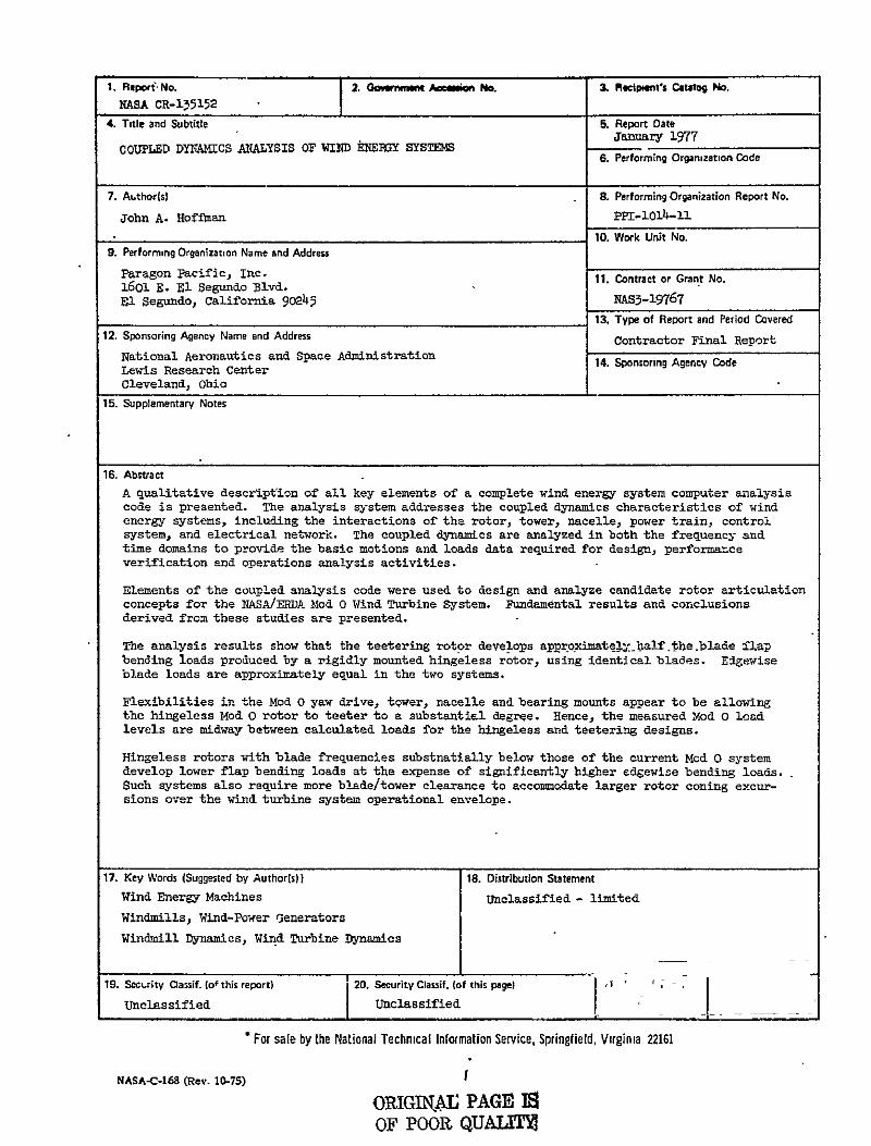
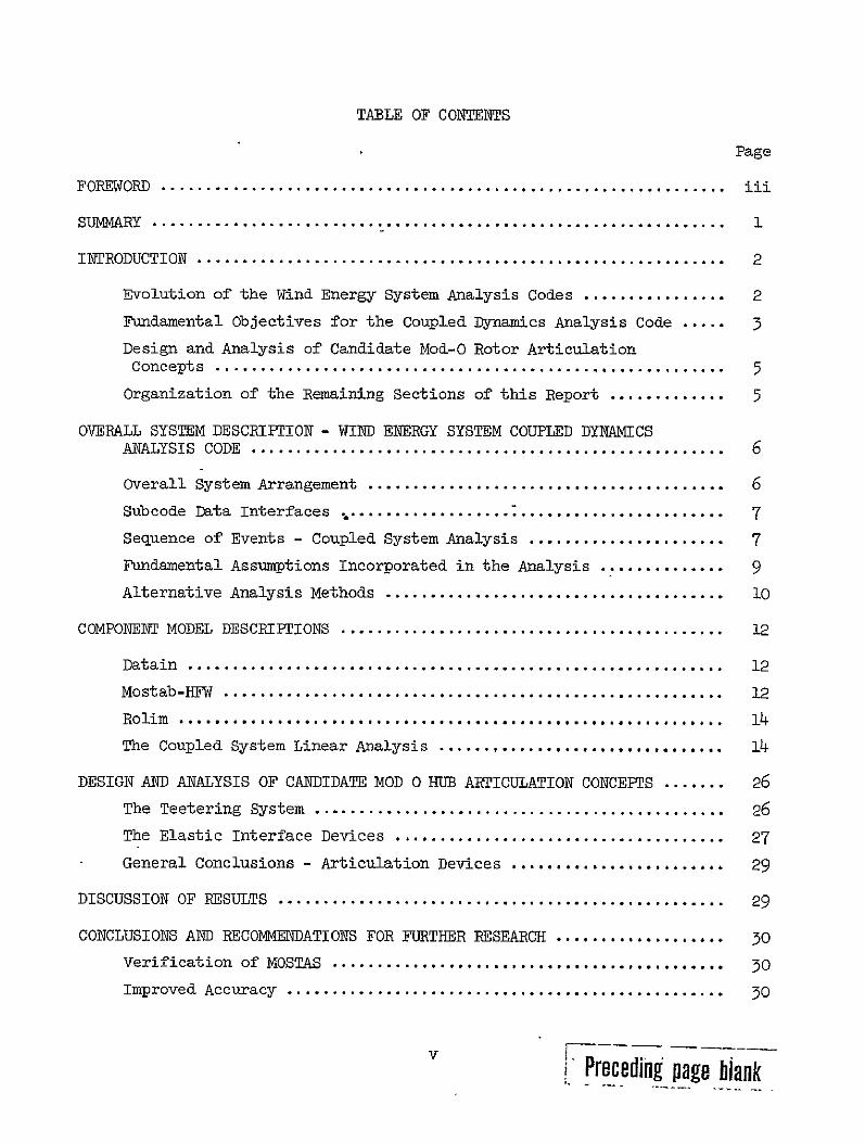
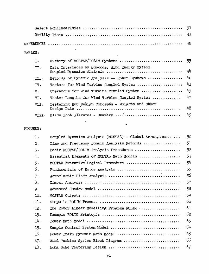
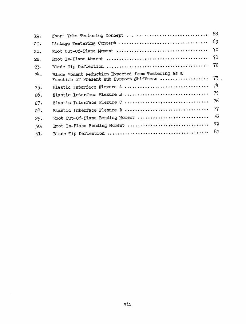
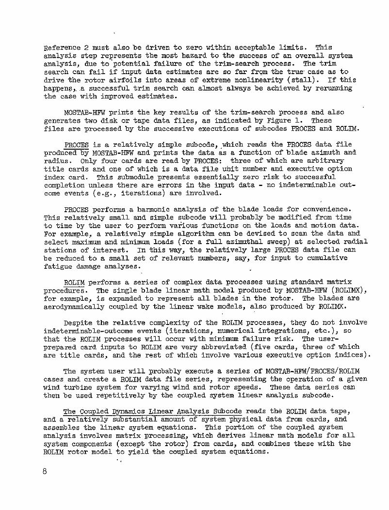
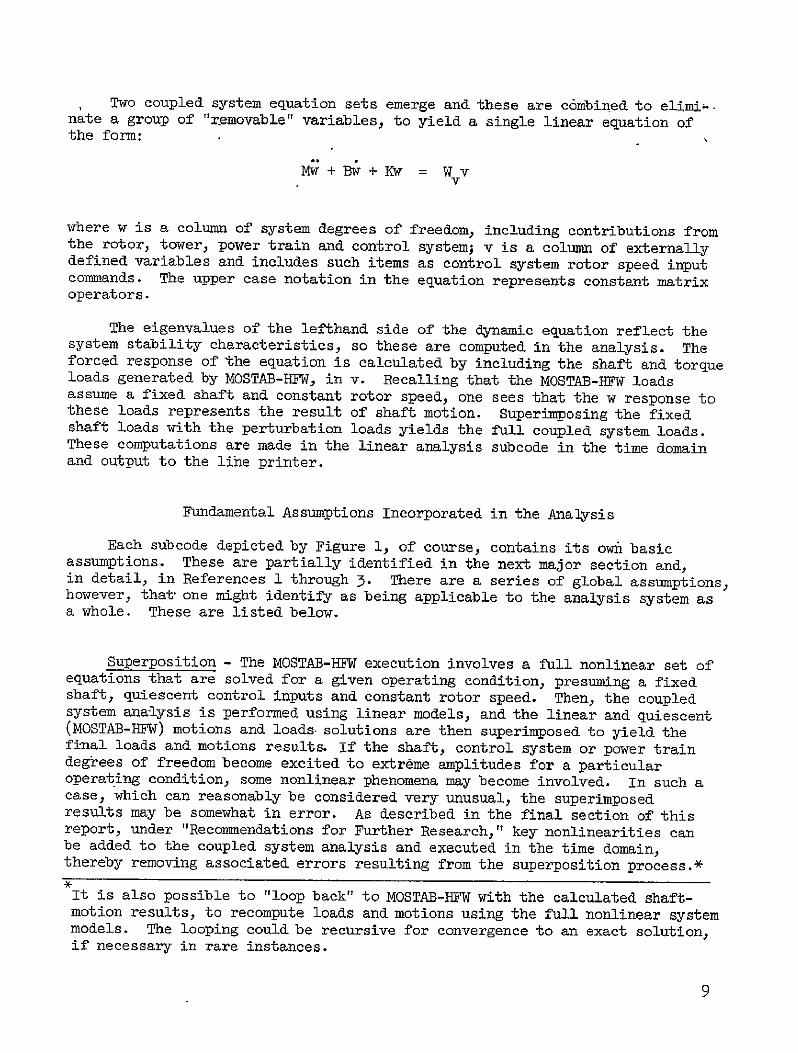
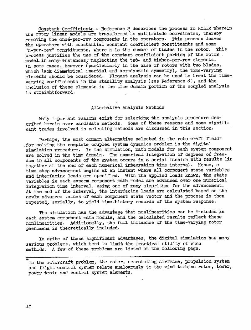
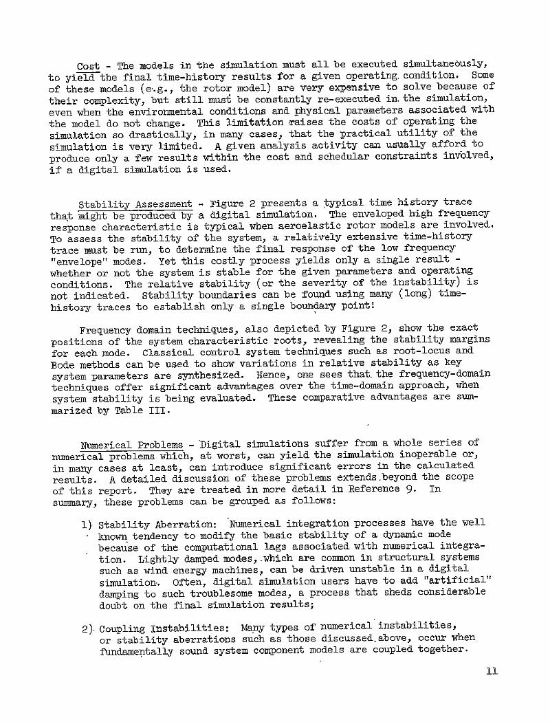
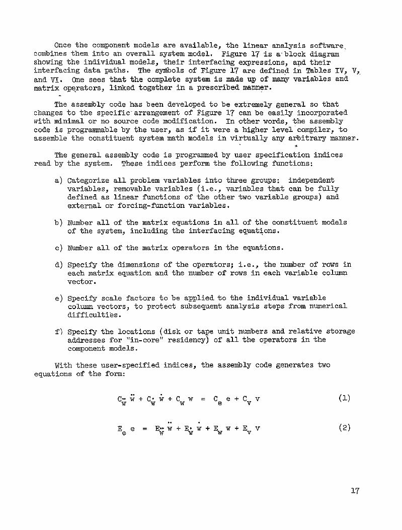
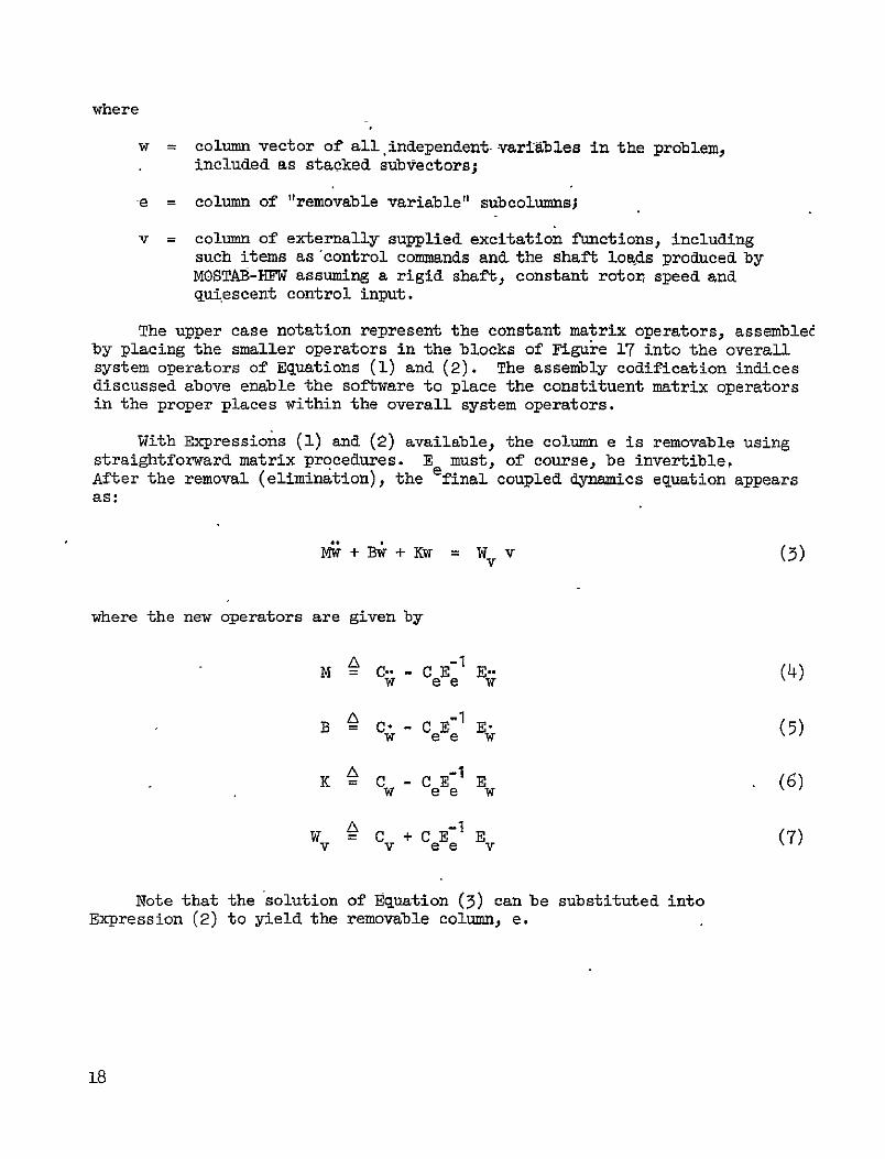
where
w = column vector of all independent- -variables in the problem included as stacked subvectors
e = column of removable variable subcolumns
v = column of externally supplied excitation functions including such items as control commands and the shaft loads produced by MOSTAB-HFW assuming a rigid shaft constant rotor speed and quiescent control input
The upper case notation represent the constant matrix operators assembled by placing the smaller operators in the blocks of Figure 17 into the overall system operators of Equations (1) and (2) The assembly codification indices discussed above enable the software to place the constituent matrix operators in the proper places within the overall system operators
With Expressions (1) and (2) available the column e is removable using straightforward matrix procedures E must of course be invertible After the removal (elimination) the final coupled dynamics equation appearsas
Mw+Bw+Kw = W v (3)
where the new operators are given by
1M CE- E- (4)w e e w
A c -CB E1 P (5)
K E-I E (6) w Cee st
WV W= v + C e E-e Ev (7)
Note that the solution of Equation (3) can be substituted into Expression (2) to yield the removable column e
18
Solving the Linear Model - Equation 65) represents the coupled system math model and can be solved using a number of different linear analysis techniques As a-general rule the operators in Equation (5) will be periodicfunctions of time since they contain contributions from the ROLIM operators which are time varying In this case the full assembly process described above must be re-executed at each rotor azimuthal station - each station represented by a different ROLIM model
The solutions to systems of linear equations are synthesized in two stepsthe homogeneous solution and the particular solution These independent steps are discussed below
1) The Homogeneous Solution
The homogeneous solution is the solution to Equation (3) with rightshyhand side set to zero The resulting equation is first reduced to first order to have the form
P= o (8)
where
P [ 0 (10)
deg0M Q [7K 1] (I)
One would wish to invert P and premultiply through by P-inverse to reduce Expression (8) to the usual characteristic equation form Because of the nature of the wind turbine system math models however P is generally singular Q will also be singular in general and the specific ranks of these arrays will depend on the detailed models used for the wind machine components
At the time of this writing the analysis system has been configured to incorporate the constant portions of the ROLIM model only in the operators of Equation (5)
19
Hence it is necessary to process Equation (8) using special procedures derived and documented in Reference 1 Singularity in P means that y is not a set of generalized coordinates In other words there are
notalgebraic constraints among the elements of y such that y does contain a full column of legitimate independent coordinates Singularity in Q means that the system contains at-least one zero
eigenvalue If q is degenerate d times then there are d zero
(repeated) characteristic roots in the system
The matrix procedures derived in Reference I essentially find a coordinate transformation matrix T such that the vector y can be
expressed as a function of generalized-coordinate column x
y = x O2)
and the dynamic equation is written
x- Mx = 0 (13)
If the constant-coefficient portion of M is used denoted herein as
Mo then Equation cL3can be processed by straightforward eigenanalysis
If the periodic constituents in M are to be included then the methods
of Floquet must be used (see Reference 8 for a discussion of the
Floquet procedure)
As mentioned previously the constant portion of M can be used to
analyze systems incorporating aeroelastic rotors in many cases with
good accuracy In this case one hypothesizes a solution to
Expression (13) of the form
x = e (14)
where x is a constant vector and 7is a scalar
Substituting this into the constant coefficient portion of
Expression (13) yields ( - M) x = 0 (15)
where the symbol f has been used to denote the identity matrix
The vector x can have a nontrivial value of course only if
Det (Xl-M) 0O (16)
20
which is easily derived by applying Cramers rule to Equation (13) Equation (16) is called the characteristic equation and values of that satisfy this scalar expression are called the characteristic roots or eigenvalues of the system
The eigenvalues j will generally be complex numbers If the system
is stable all the values will have negative real parts If one or more A values have positive real parts substitution into Equation (14) clearly shows that the system is unstable
For each eigenvalue Aj there will generally be a corresponding
eigenvector xj that is found using the eigenvalue and a pivoting
numerical procedure on Expression (15)
If a Floquet procedure is used characteristic roots 7 are found
that represent the basic eigenvalues of the system with periodicityincluded in the analysis
The eigenvalues are very important to the system dynamics They show the stability (or lack thereof) of each coupled mode in the system and the relative degree of stability for each mode
The eigenvectors show the participation of the various system components in each mode For example the j eigenvector defined as
y T xj (17)
shows the coordinates in y involved in the jth mode of motion If 7 is an unstable eigenvalue then 7 would reveal which coordinates of 0
the system are involved in the instability helping to lead the system designer to an understanding and hopefully a correction of the instability
2) The Particular Solution
The particular solution of Expression (3) involves solving for a specific time variable w(t) for a given forcing function v(t) Then the general solution is a superposition of the homogeneous and particular solutions
One special case of interest in the wind energy system analysis involves the particular solution of Equation (3) in response to a periodic forcing function v This case is particularly important in solving for the moving shaft system loads In this case v contains the periodic shaft and torque loads generated by MOSTAB-HFW assuming the fixed shaft constraint These loads will appear in v so that v can be written
21
N jiv(t) = V e lt (18)
where J is defined in this case as--the- cblex operator
bullSince -Expression(3) is linear it -can be solved for eachtharmonic component of v considered separately and the independently derived solutions can then be-superimposed
To see this consider again the constant coefficient form bf Expresshysion (3) Assume a solution to the ith harmonic excitation from v of the formshy
i tW = V er n (19)
Substituting Expressions (18) and (19) into the constant-coefficient portion of Equation (3) yields
(_i2n2M0+ injB6 + K0) Wi e~it = WvVi eJint (20)
or
D (a) Wi = WvV1 (21)
where
D (n) 5 (Io - i20 0 ) + j(iaBo) (22)
The complex array D is generally nonsingular yhence
1Wi = D-1 (c)Wv (23)
Then the harmonic response to v is given by N
ji tt) = w e n (24) i=l 2
22
Equation (24) reveals the coupled system response to the fixed-shaft loads produced by MOSTAB-HIW Superposition of the function w(t) with the corresponding variables calculated by MOSTAB-HW yields the complete coupled system response with a free shaft and variable rotor speed
The procedure described above leading to harmonic response Expresshysion (24) is the process currently incorporated in the coupled system analysis to produce free-shaftspeed time-history responses
Many alterations and extensions to this method could easily be included in WINDLASS as added developments Two such extensions are discussed below
3) The General Solution (Summary)
Many alternative time-domain solutions can be implemented using the basic dynamic Equation (3) One must use caution in implementing linear analysis procedures however and reflect on the facts that M and K are generally singular and that all the operators are periodic functions of time Two practical extensions of the methods currently implemented in the coupled analysis are presented below
Either method would first convert Expression (3) to its first order form
Py-Q R v (25)
where Definitions (9) through (11) are used with
R 0 (26)
The first procedure would simply solve Expression (25) as a constantshycoefficient expression over time intervals equivalent to one rotor azimuthal station Each successive azimuthal advance in the value of y would use entirely different linear operators properly reflecting the periodicity in these operators
To develop this method one may proceed with a constant-coefficient analysis of Expression (25) since this will only be used for one azimuthal sector advance An immediate problem is encountered however due to the fact that P is singular so that one cannot solve directly for y
23
To solve this problem the methods of Reference 1 are used to find the eigenvalues of the homogeneous portion of Expression (25) The eigenvectors are also found and stacked column by column inan-array Y called the modal matrix As discussed in Reference 1 another modal matrix Z can be derived -such that Z is the matrix of eigenvectors -for the transposed system
T 0 (27)
The eigenvalues of Equation (27) will be identical to those found for the homogeneous portion of Expression (25) since transposition of a determinant (Equation (16)) does not change its value
Now specify the coordinate transformation
y = Y q (28)
and transform Expression (25) accordingly Then premultiplying by the transposed system eigenvectors yields
(z T PY) - (ZT QY) q = (ZT R) v (29)
Reference 1 proves that the two operators on the lefthand side of Equation (29) are diagonal matrices and they are nonsingular Also Equation (29) can be written
q -Aq =P v (50)
where
P (czT PY)- 1 ZT R (51)
and
ZTA = (Z T PY)-1 QY (32)
The diagonal matrix A as shown by Reference 1 has the system eigenvalues as its diagonal elements
The array Pv might be called the matrix of participation factors
since it determines how the forcing function elements in v participate in the excitation of each normal mode in the system Coordinates q which are generally complex are called normal coordinates
24
Equation (30) is solved in a straightforward manner for any arbitrary forcing function v(t) given some initial condition q () valid at time t = r Once q(t) is knownthe orlginl coordinates y are recovered from transformation Equation (28) -
The second procedure for solving Expression (3) in the time domain including the time-varying operators is derived using the results of the first method However it does not require eigenanalysis at each rotor azimuthal station Rather the operators of Expression (25) are separated into constant-coefficient and time-varying component constituents The time-varying parts are transposed to the righthand side of the equation and treated as forcing functions The result is
Poy p v- Py + y (33)
where the barred arrays have zero mean values Now the entire process described for method number I is executed using the arrays P and Qo
Transformation Expression (28) is still valid and the diagonal Expression (30) emerges in the form
q- Aq Pv v + p + p q (34) v q q
where
P 4 (zT PY) 1 zT PY (5)
qa
and
1pq 4 + (zT PoY) ZT Y (56)
Equation (34) can be solved in a straightforward numerical fashion with periodic arrays P P4 and P known and using the constant diagonal
q qarray A (the eigenvalues associated with P0 and Qo)
In conclusion the method of Equation (24) has been incorporated in the current coupled analysis system for time-domain examination The alternative procedures described above can be implemented in a relatively straightforward manner however using the coupled system Equations (1) and (2) and standard linear analysis subroutines incorporated in the current system
25
DESIGN AND ANALYSIS OF CANDIDATE MOD 0 HUB ARTICULATION CONCEPTS
A portion of the subject contractual activity dealt With the design and analysis of two hub articulation concepts for the Mod 0 Wind Turbine teetering and elastic interface devices Both concepts were investigated for their potential to reduce bladeloads in the baseline Mod 0 design and both were synthesized to involve a minimum of modification to existing Mod 0 hardware
This section presents some of the more promising design concepts identified during the study along with key analytical results and conclusions associated with them
The Teetering System
Description of Concepts Considered - Figures 18 through 20 present the conceptual designs considered for the teetering systems The system of Figure 18 places the teetering hinge forward of the point of shaft intershysection with the blade centerlines at approximately the overall rotor center of gravity point Teetering helicopter rotors place the teetering hinge at approximately the eg point of the blades alone which in the case of the Mod 0 would be about 091 meters (three feet) from the blade centerline intersection point Placing the hinge outward in this fashion is called undersling in the helicopter vernacular rotors are underslung to reduce the magnitude of Coriolis inplane excitation loads due to rotor teetering The undersling shown in Figure 18 tends to reduce the Coriolis loads and additionally balances the complete rotor assembly for easy handling and quiet operation at near-zero speeds
Figure 19 is the short yoke design which makes no attempt to balance the rotor or to reduce Coriolis loads It is much simpler and lighter than the long yoke however
Figure 20 presents a linkage design which does not require a long yoke to project the virtual teetering axis well forward of the blade centerline intersection point The device has the characteristic however that the virtual teetering axis does not stay stationary with respect to the shaft but translates in an essentially vertical are as the rotor teeters
Table VII lists the weights and other design data associated ith the teetering concepts shydeg
Analysis Results for the Teetering System - Figures 21 through 25 present the key MOSTAB-HFW analysis results derived for the teetering concepts Remembering that these results incorporate the fixed shaft assumption the following observations are made
26
a) The flapwise bending loads in the teetering systems are roughly half those in the baseline (hingeless) Mod 0 design regardless 6f hinge point location
b) The gravity loads in the inplane direction are so large that the Coriolis loads are relatively small by comparison Hence undershysling to reduce Coriolis loads as done in helicopters is probably of little positive consequence in the Mod 0 system
c) The flapwise loads remaining in the teetering rotor blade shanks are of even-per-rev harmonic content the odd-per-rev constituents (present in the baseline Mod 0 system) being removed by teetering (as would be expected)
d) The teetering response (Figure 23) to the shadow excitation has its maximum upwind displacement at roughly 4f= 90 degrees as would be expected and the teetering arrangement maintains the basic Mod 0 precone Hence the teetering concept does not tend to allow the blades to approach significantly closer to the tower than in the baseline Mod 0 design A gust with a verticdl axis such as might occur during thunderstorm activity might teeter the rotor toward the tower however
Although the fixed-shaft analysis indicated that the teetering design could reduce flapwise bending loads by half further examination of available Mod 0 test data indicated that the Mod 0 system is already teetering to a significant degree due to flexible shaft supports Such flexibility probably arises from a combination of bearing tower pod and yaw drive flexibilities Figure 24 shows the predicted reduction in baseline Mod 0 flapwise loads for the teetering system including the partial reduction already made by flexible supports This curve indicates that a teetering hub will probably reduce existing Mod 0 loads by only about 50 percent based on estimates of the average shaft support flexibility
Since the coupled system dynamic analysis was not available for the teetering study the results of Figure 24 were not tested with this new and more general computer code The results are compatible with Mod 0 test data however lending them considerable credibility
The Elastic Interface Devices
Explanation of Candidate Devices - Figures 25 through 28 present four elastic interface devices which could be simply bolted on to the existing
An intuitive explanation of this important result is that when one blade passes through and responds to the shadow wake (the source of greatest dynamic excitashytion) the neighboring blade fails to respond significantly ie the blade in clean air maintains a particular response trajectory regardless of its root loads Hence both blade shanks share the deflection required by the response of the blade leaving the shadow region reducing the loads in both shanks by one half
27
Mod 0 system between the blade root flanges and the hub All four devices are essentially flexures that reside substantially inside of the existing Mod 0 blade and cliff assemblies As such they add only 152 centimeters (5 feet) to the Mod 0 rotor radius
Two of the flexures are steel and two are unidirectional fiberglass Table VIII presents key design and loads data associated with these designs indicating that the fiberglass units are superior particularly from a fatigue standpoint
One of the fiberglass flexures is symmetrical having equal stiffness in all directions of bending The rectangular section has been arranged for more stiffness in the plane of rotation than out of the plane The unfortunate fact that the blade feathering hinge is inboard the flexures however means that the flexure principal axes rotate with respect to the rotational plane with rotor feathering Feathering angle is of course a function of wind and rotor speed and power level
Analysis of the Flexures - An analysis was performed to determine the modeshapes and frequencies of the bladeflexure combination as a function of flexure design and feathering angle These results were then input to MOSTAB-HFW to solve for the resulting blade loads and motions Figures 29 through 31 show key MOSTAB-BFW results applicable to the symmetric and asymshymetric fiberglass flexure designs depicted by Figures 25 through 28 A few conclusions that can be derived from these analysts results are
a) Flapwise bending loads are reduced by the relatively soft flexures by 50 percent for the symmetric flexure and 60 percent for the asymmetric flexures
b) Because of the low inplane natural frequencies of the symmetric and asymmetric flexures (15 P and 191 P respectively) compared to the stiff Mod 0 inplane support (36 P) the dynamic inplane loads are seriously aggravated by the flexures The one-per-rev gravity loads and the dynamic amplification associated with this 1 P load acting closer to resonance than in the baseline Mod 0 system is undoubtedly responsible for these increased loads
c) As might be expected the asymmetric flexure with its higher inplane frequency has improved inplane loads over those developed by the symmetric flexure
d) Because the soft flexures cannot maintain precone as is possible with the teetering design gusts or operation at full speed and low power levels can beexpected to uncone the rotor into the tower Hence the flexure concept will generally require more bladetower clearance than the teetering concept probably to the point of requiring a shaft tilt to swing the blades well clear of the tower
28
As was the case with the teetering analysis the coupled analysis computercode was not available for the flexure device examinations All these studies were conducted with the fixed-shaft and constant rotor speed assumptions
General Conclusions - Articulation Devices
The teetering articulation can be expected to reduce blade flapwise loads by roughly half for systems with very stiff shaft supports with softer systemssuch as the baseline Mod 0 design the loads reduction can be expected to be less In the case of the Mod 0 system a teetering rotor can reduce flap loads by about 50 percent with relatively minor impact on inplane loads Since the teetering concept retains precone it does not tend to aggravate tower clearance margins although certain types of gusts can be expected to teeter the rotor into the tower
The flexure devices offer the most potential for reducing flapwise loads but a high inplane stiffness is required to avoid paying a severe attendant penalty in inplane loading The problem of maintaining a small ratio between flap and inplane flexural bending stiffnesses is exacerbated by the location of the feathering hinge inboard of the flexures Because the flexures are soft the wind turbine rotor shaft should be tilted if they are incorporated to provide ample bladetower clearance
It should be noted that rigid rotor blades are all essentially flexureswith the flexural elements integral with the blade Future wind turbine blade design activities should address the concept of making the flap stiffnesses lower while maintaining a high inplane stiffness to achieve the benefit of the soft flexure on flap loads without the penalty on inplane loads Also the softer (flapping) blades will require more tower clearance not so much because of dynamic flapping but because of static coning
DISCUSSION OF RESULTS
Because the subject contractual activity has been executed in distinct subactivities the discussions of results appear in previous sections of this report
Results associated with the Mod 0 articulation concepts were presented in the section entitled Design and Analysis of Candidate Mod 0 Hub Articulation Concepts
29
CONCLUSIONS AND RECOMMENDATIONS FOR FURTHER RESEARCH
A complete coupled analysis software system has been developed for application to a broad range of wind energy machine designs The system addresses wind machine dynamics in both the frequency and the-timel domaifs and includes the-interactions of the rotor nacelle power train control system and electrical equipment
Based on the current status of the work supported by the subject contract a number of additional developments can be recommended which would enhance the accuracy and utility of the wind energy system coupled dynamics analysis A few of these are presented below
Verification of MOSTAS
The fundamental purpose of the subject contractual work was the developshyment of the wind energy system coupled dynamics code MOSTAS Example MOSTAS executions presented in Reference 3 were prepared for check cases to be run when MOSTAS is brought up on a given computer system The examples configured specifically to check the code are not satisfactory for analysis system verification
Accordingly a very important future step in the MOSTAS development process would be verification of computed results by comparison with available test data It is anticipated that such comparisons will be madeusing Mod 0 test data in the very near future
Improved Accuracy
The section entitled Component Model Descriptions identified procedures for rigorous treatment of the time-varying constituents in the coupled dynamics equation operators These include Floquet analysis for the frequency-domain examinations and advanced numerical integration procedures for the time domain analysis It is highly recommended that these advanced procedures be incorshyporated in the code
Some key areas of the dynamic analysis code should be typed double precision particularly if they are to handle large systems
Paragon Pacific Inc has a procedure called the Root Perturbation Method which is expected to yield the Floquet roots of large periodic systems without the usual numerical problems associated with Floquet analysis Upon development this new method should be implemented in the wind energy system analysis
30
Select Nonlinearities
The coupled system code is capable of solving for dynamic responses with the presence of key system nonlinearities such as gear backlash control system linkage hysteresis and power train nonlinear damping and flexibilities In the event that such analysis results are needed to support the developmentof wind power machines MOSTAS should be extended to include the nonlinearities of interest
Utility Items
A number of convenience items might be added to the coupledsystemanalysis considerably enhancing itsutility A few items inthis category are
a) Plot packages
b) Input data check codes examining the boundaries of user-specifieddata for compatibility with available storage allocation and other program constraints
c) Miscellaneous improved and extended print formats
In addition to the recommendations forwarded above for the dynamicanalysis software it is recommended that the key conclusions reached during the hub articulation design and analysis activities be re-examined using the full coupled system analysis in lieu of the basic fixed-shaft analysis methods
Lewis Research Center National Aeronautics and Space Administration
Cleveland Ohio 44135 January 1977
31
REFERENCES
1 Henninger William C Hoffman John A and Williamson Dale R Mathematical Methods Incorporated in the Wind Energy SystemCoupled Dynamics Analysis Part I - Basic Methodology for the Modular Stability-Derivative Program (Revision B) Part II -Analysis Methods Incorporated in the MOSTAB-HFW Computer Code Part III - Methodology Wind Turbine Linear Analysis Software System (WINDLASS) PPi-Io14-7 Paragon Pacific Inc January 1977
2 Henninger William C and Hoffman John A Analysis Methods Incorporated in the Rotor Linear Modelling Program (ROLIM)PPI-2001-2 Paragon Pacific Inc October1976
3- Henninger William C Hoffman John A and Williamson Dale R MOSTAS Users Manual Volume I - Users Manual for the Modular stability Derivative Program - High Frequency Wind Turbine Version (MOSTAB-HTW) PPI-1014-8 Volume II - Users Manual for the Wind Turbine Linear Analysis Software System (WINDLASS) PPI-lOl4-9 Paragon Pacific Inc January 1977
4 Hoffman John A Wind Turbine Analysis Using the MOSTAB Computer Program MRI Report 2690-1 Mechanics Research Inc 1974
5 Janetzke D C Puthoff R L and Richards T R Rotor Pershyformance Predictions for the 10OKW Experimental Wind Turbine Preliminary report NASA Lewis Research Center
6 Spera David A Structural Analysis of Wind Turbine Rotors for fSF-NASA Mod-O Wind Power System NASA TM X-3198 1975
7- Williamson Dale R Design of Articulated Hub Concepts (Final Report) Volume I - Teetering Volume II - Flexures PPI-l0l4-lO Paragon Pacific Inc January 1977
8 Hohenemser Kurt H and Sheng-Kuang Yin Some Applications of the Method of Multiblade Coordinates Journal of the American Helicopter Society vol 17 no 3 July 1972
9 Hoffman John A Some Practical Aspects Associated withiDigital Execution of Rotorcraft Math Models for Time-Domain Simulation PPI-3010 Paragon Pacific Inc November 1976
10 Hurty Walter C and Rubinstein Moshe F Dynamics of-Structures Prentice-Hall Inc 1964
11 Glasgow J C (5252Wind Power Office) Memorandum to Wind Turbine Dynamics Review Committee Subject - SelectedMod-O Experimental Wind Turbine Operational Data (unpublished) NASA Lewis Research Center Cleveland Ohio March 4 1976
32
TABLE I- HISTORY OF MOSTABROLIM SYSTEMS
TIME PROJECT
1965-69 DEVELOPMENT OF ROTOR MATH MODELS
DIGITAL AND ANALOG SIMULATIO (ORIGINAL REXOR CODES)
1969-72 ORIGINAL MOSTAB DEVELOPMENT FOR-ROTORCRAFT ANALYSIS MOSTAB-B
MOSTAB-C MOSTAB-CR AND MOSTAB-HIV VERSIONS CODES PUBLISHED AND PUBLIC DOMAIN
1972-74 MOSTAB VERSIONS EXPANDED FOR BLOWN ROTOR AND AEROELASTIC ANALYSIS MOSTAB-CCR (CIRCULATION-CONTROLLED
ROTOR)
MOSTAB-HFA (HIGH FREQUENCY ANALYSIS)
1973-74 BASIC MOSTAB-CR REFINED FOR WT ANALYSIS
1974-75 ROTOR LINEAR MODELLING CODE (ROLIM) DEVELOPED-
1975 DATE
TO MOSTAB-HFA EXTENDED TO MOSTAB-HFW
FOR COUPLED WT-ANALYSIS
1975 TO
DATE
MOSTAB-HFA
ANALYSIS
EXTENDED FOR X-WING
SUPPORT
LOCKHEED
IRAD
US ARMY
(EUSTIS)
NASA
(LANGLEY)
US NAVY
(NAVAIR MONITORED-
BY
]TNSRD)
NASA (LEWIS)
PARAGON PACIFIC IRAD
NASA
(LEWIS)
US NAVY
33
TABLE II - DATA INTERFACES BY SUBCODE WIND ENERGY SYSTEM COUPITED DYNAMICS ANALYSIS
SUBCODE DATAIN
Input Data Required
Basic MOSTAB input data from cards
1 Physical features of each component -
Earth Effective aerodynamic area and drag coefficient
Tower Effective aerodynamic area and drag coefficient
Rotor - Miscellaneous indices describing numerical sector sizes - Nominal speed - Radius - Angular orientation with respect to other wind machine
elements - Radial schedules geometry
chord twist coning shape
- Radial schedules mass properties
distributed mass S so center of gravity location
o blade-section inertiatensor -
- Radial schedules dynamic prqperties modeshapes - Frequencies for each Uladeiddo shy
- Numerical integration procedure for each blade mode - Gimbal propertie if applidable (gimbal tyipe
Lt- distance and teeterpitchcoupling)undersling
2 Relative locations of each compgnent in the overall system
3 Aerodynamic interference model properties-
Wake properties
Wake coupling coefficients
ltShadow wake -profiierdefinition --
4 Operational conditions -
Wind speed
Air properties (density- temperatur etc)
Rotb precession rates
34
TABLE II - Continued
5 Miscellaneous numerical indices (numerical differentiation increments etc)
Output Data Produced
1 Formatted printed input data (line printer)
2 Unformatted binary data file for input to MOSTAB (sequential access disk or tape file)
SUBCODE MOSTAB-HFW
Input Data Required
1 Data file unit definition and executive option flag (card)
2 Binary file produced by subcode DATAIN (disk or tape)
Output Data Produced (Line Printer)
1 Essential constant data for rotor analysis generalized masses completed modeshape functions etc
2 Results of successive trim-search passes
3 Results of successful trim search -
Rotor average shaft loads produced for trim (resolved to a nonrotating coordinate system)
Wake velocity components (eg retardation velocities) developed at trim
Average power produced
4 Gradient arrays showing rotor shaft load responses to variations in relative wind speed components shaft precession rates and rotor control variations
Output Data Produced (PROCES File - Sequential Access Tape or Disk)
1 Rotor blade motion data at trim - blade modal coordinates and their time derivatives as a function of blade azimuth
35
TABLE II - Continued
2 Gimbal degrees of freedom motions and their time deri-vatives vs azimuth (if applicable)
3- Rotor blade internal loads vs radius and azimuth
4 Shaft loads produced by one blade vs azimuth
5 Aerodynamic distributed loads data vs radius and azimuth including angle of attack mach number dynamic pressure lift drag and moment coefficients and distributed force and moment air loads
Output Data Produced (ROLIMX File - Sequential Access Tape or Disk)
1 Basic geometric and trim-search data -
Relative geometric location of elements in wind turbine system
Mass properties of rigid body mass elements associated with system
Trim-search loads results
2 Linear math model for a single rotor blade -
Shaft loads
Gimbal error function (if applicable)
Generalized forcing function applied to blade modes
These linear math models appear as gradient arrays operating on all blade and shaft degrees of freedom and on control and rotor speed input functions and their time derivatives The gradient
arrays are functions of azimuth
3 Linear math models representing the aerodynamic couplings among the aerodynamic elements of the wind turbine system
SUBCODE PROCES
Input Data Required
1 Data file unit numbers and executive option indices (card)
2 PROCES data file produced by MOSTAB-HFW (see MOSTAB-HFW output data produded PROCES data file above)
36
TABLE II - Continued
Output Data Produced (Line Printer)
1 Formatted printout of the basic trim loads and motion data on the PROCES input data file
2 Internal blade loads and shaft loads produced by a single blade by frequency component (harmonic analysis results performed by PROCES)
Output Data Produced (Card Punch - Optional)
Harmonic blade and shaft loads
SUBCODE ROLIM
Input Data Required
1 Data file unit numbers executive option indices and harmonic and time-point specifications on ROLIM output data (card)
2 ROLIMX data file produced by MOSTAB-HFW (see Subcode MOSTAB-HFW Output Data Produced above)
Output Data Produced (Line Printer and Sequential Access Tape or Disk File)
Linear math model of rotor system including all blades aerodynamically coupled (and mechanically coupled in the case of gimballed rotor analysis)
1 Model arrays operating on rotating coordinates and expressed as a function of azimuth position
2 Same as 1 except expressed as sinecosine Fourier aoefficients
3 Same as 2 except expressed as amplitudephase angle Fourier entities
4 Model arrays transformed to operate on multi-blade coordinates shymodels have reduced one-per-rev components - expressed as functions of blade azimuth position
5 Same as 4 except expressed in sinecosine Fourier coefficients
57
TABLE II - Continued
6 Same as 5 except expressed in amplitudephase angle Fourier entities
SUBCODE COUPLED DYNAMIC SYSTEM LINEAR ANALYSIS (WINDLASS)
Input Data Required (Tape or Disk File)
Type 4 output data produced by ROLIM linear rotor math model operating on multi-blade coordinates and expressed in sinecosine coefficient form (tape or disk file)
Input Data Required (Cards)
1 Data file unit definition and executive option flags
2 Executive specification indices which define by code -
Input data items
Independent variables to be included in the coupled system dynamic equation
Dependent variables associated with the coupled system dynamic equations
Variables defined as removable ie variables included in the elemental formulations of the linear math models which are to be ultimately calculated but which can be eliminated from the basic coupled system dynamic equation
Miscellaneous other executive specification indices
3 Physical data associated with each component of the wind energy system excluding the rotor -
Tower Modeshapes frequencies and mass properties base flexibilities inertia and damping properties dimensional geometry
Power Train Inertia stiffness damping and gear ratio coefficient
associated with each building block in the power train specification indices which link the power train building blocks
38
TABLE II - Concluded
Control System (Model includes dynamic characteristics of power
machinery power machinery controls power generating reflected torques and network elements) -Loop specifications transfer functions and gains
Pod (Nacelle) - Stiffness and inertia properties geometry at rotor tower and power train interface locations
4 Harmonic coefficients required to define dynamic shaft and blade loads produced by subcode PROCES
Output Data Produced (Line Printer)
1 Linear operators in ccupled system dynamic equation
2 Linear operators in removable variable equation (solvable from results of coupled system dynamic equation)
3 Eigenvalues and eigenvectors (reflecting coupled system stability) computed from the homogeneous portion of the dynamic equation
4 Time-history responses of selected system independent and removable variables representing the coupled system perturbation responses from the trim condition responses calculated by MOSTAB-HFW
5 Time-history responses periodic blade root loads superposition of trim loads computed by MOSTAB-HFW and perturbation coupled dynamic loads
39
TABLE III - METHODS OF DYNAMIC ANALYSIS-- ROTOR SYSTEMS
ADVANTAGES DISADVANTAGES
TIME-DOMAIN SIMULATION
s MANY DOF AND NONLINEARITIES EXCESSIVE COMPUTER COSTS
CONSTANT RE-SOLUTION FLEXIBLE PROGRAMMABILITY DIFFICULT STABILITY
EVALUATIONS NUMERICAL INSTABILITY
HAZARD
FREQUENCY-DOMAIN SOLUTION STANDARD PROCEDURES
CLEAR STABILITYEVALUATION CONSTANT COEFFICIENTS REQUIRED
-e-COMPONENT MODELS QUASI-STATIC ASSUMPTION
MOSTABROLIM SYSTEM
ALL ADVANTAGES OF REQUIRES FLOQUET OR FREQUENCY-DOMAIN ROOT-PERTURBATION
STABILITY ANALYSIS - METHOD ANALYSIS LINEAR ANALYSIS
PERIODIC MATH MODELS HNIGH FREQUENCY ROTOR
MODES
4o
TABLE IV - VECTORS FOR NIND TURBINE COUPLED SYSTEM
DescriptionaSymbol
c c c Control system inputs to rotor (NC)
f Perturbation load on rotor due to freeing fixed shaft (6)
fEP External load applied to pod (mP6)
fEPR Load at podrotor interface point applied topod (6)
fEPT Load at podtower interface point due to elasticdeformation of pod (6)
(NT6)fET External loads applied to tower
fH Total load on moving hub at rotorpod interfacepoint (6)
(6)fTP Load at podtower interface point applied to tower
fo Fixed shaft load applied to hub mass - from MOSTAB-HFW(6)
f Total moving shaft load applied to hub mass (6)0
h2 b External inputs to control system (iH)
x x x Rotor shaft perturbation motion (6)
X p Pod grid point displacements (NP6)
XT xT Displacement acceleration of tower grid points (NT6)
xTr7 p Displacement icceleration of towerpod interface point (6)
y Rotor degrees of freedom (NY)
a Control system degrees of freedom (NA)
YB Power train gear box reaction torque applied to pod (NBOX)
7C Control system torque applied to power train (1)
7cp Control system torque applied to pod (NGCP)
aItems in parentheses are vector length (see Table VI)
41
TABLE IV - Concluded
Symbol Description
rEP
7RPT
sect
(Power
CRPTV cPFT
External torque applied to power train (NPHI)
Power train torque applied to rotating hub mass
Tower base degrees of freedom (5 or 6)
Tower modal coordinates (NMv)
train independent degrees of freedom (NrnI)
Rotor rotation speed and acceleration perturbations (1)
()
4j
bull j
Rotor azimuth angle (1)
Rotor speed and acceleration perturbations (1)
42
TABLE V - OPERATORS FOR WIND TURBINE COUPLED SYSTEM
Symbol Description
AUo Control system operators
B3 BEQ BNj Damping operators for power train equations
BP BRW BC
B h) Control system operators for external input h
BI B B- Y Y y
Control system operators for rotor degrees of freedom y
B B Control system operators for rotor velocity and acceleration a
D D- Relate control system degrees of freedom to rotoraYcontrol variables
ECp Rotational transformation and partitioning operator for control system torques applied to pod
EEX Rotational transformation matrices for externally applied pod loads
Rotational transformation operator for pod loads at
EpR the rotorpod interface point
EppT Rotational transformation and partitioning operator for power train gear box torques applied to pod
ETp Rotational transformation matrix to express tower loads and deflections in the pod reference system
EXp Rotational transformation and partitioning operatorPR for pod deflections at the rotorpod interface point
E Relates control system degrees of freedom to generatora torque
FT Tower modal force participation factor for external tower loads
F Tower modal force participation factor and partitioning I operator for load at towerpod interface point
43
TABLE V - Continued
Symbol Description
G
GI
Tower grid point geometric operator for exterhal tower loads Tower grid point geometry and partitioning operator
for load at towerpod interface point -
GT Tower grid point geometric operator for external tower loads
IC Partitions generator torque 7yC reaction to appropriate gear box
IEP Partitions main gear torques to power train dofs
IEPT Applies the podtower interface load to the approprpod degrees of freedom
te
IPF
PT
Partitions reactions applied by the rotor to the pod
Partitions out those pod degrees of freedom at the podtower interface point
XO Partitions fixed shaft loads fo to rotorpod interface point
I
IXT
Partitions fixed shaft torque from f to power train
Partitioning operator for motion of towerpod interface point
Partitions out the five rotor shaft displacements that ate compatible with the pod
Y I Iy
Partitioning operators for moving shaft degrees of freedom
JB JP5
J
JEQ JN
JR JqP
Inertia operators for power train equations
Effective inertia of tower base including mass
by tower
loading
JH Rotor polar moment of inertia
44
TABLE V - Continued
Symbol
JX
K
B KEQ KN Kp) KR -K (
KpPPod
KO
M
MH
Ma
M
P
P
Q RcR R
Rf
Rj
U
UB
Description
Partitioned rotor polar moment of inertia
Power train shaft torsional stiffness operator or tower base stiffness operator
Stiffness operators for power train equations
stiffness operator or power train stiffness operator Differential stiffness operator for fixed shaft load in moving hub coordinate system
Rotor acceleration operator from ROLIM
Non-spinning rotor hub mass matrix
Pod mass matrix transferred to towerpod interfacepoint
Tower grid point mass loading on tower modes
Tower modal mass loading on tower base
Rotor velocity operator from ROLIM
Relates control system response to torques on the pod
Rotor displacement operator from ROLIM ROLIM operators for applying control inputs to rotor
ROLIM operator for applied rotor shaft load
ROLIM operators for changes in rotor speed andacceleration
Unity 6 x 6 operator
Unity operator for power train gear box torquereactions
45
TABLE V - Concluded
Symbol Description
U Unity-operator for rotor controls c c and -
UCp Unity operator for control system torque reaction to pod 7 Cp
UT Unity operator for tower degrees of freedom
U Unity operator for tower modal degrees of freedom
U1 Unity I x 1 operator
W Tower modal frequency operator
X Tower mode shapes fixed base
46
TABLE VI - VECTOR LENGTHS FOR WIND TURBINE COUPLED SYSTEM
Symbol Description
NA Control system degrees of freedom
NB Tower base degrees of freedom (5 or 6)
NBOX Power train gear boxes
NC Rotor control degrees of freedom
NEV Eigenvalues in tower modal model
NGCP Interface degrees of freedom between pod and control system
NH External inputs to control system
NPHI Power train gear block elements and independent degrees of freedom
NP6 Pod degrees of freedom (6 times the number of grids)
NT6 Tower degrees of freedom (6 times the number of grids)
NY ROLIM rotor model degrees of freedom
47
TABLE VII - TEETERING HUB DESIGN CONCEPTS - WEIGHTS AND OTHER DESIGN DATA
Teetering concept
Weight a outboardShifto Hub (M
Undersling )
Stop Mechanism
Description Comments
Long Yoke 15100 -0178 0478 Hydraulic Cylinders
Long yoke places teetering axis near overall cg
Requires modified outboard hub plateheaviest concept
Short Yoke 9800 0178 -o386
Hydraulic Cylinders
Short yoke places teetering axis near shaft face for minimum weight
Negative undershysling is unconventi6nal
Linkage 10200 0381 O914 HyIdraulic Cylinders
Basic four-bar linkage places teetering axis at classical under-slung location
Least conventional teetering aais translates slightly as linkage moves
a Stop mechanism not included
TABLE VIII - BLADE ROOT FLEXURES - SUMMARY
DESIGN
Material Modulus of Elasticity (1010 Nm2 ) Dimensions (m) Flexure Weight (N blade) Total Assembly Weight (N blade) Divergence Speed msec from TE 45 degrees
Inplane Natural Frequency (per-rev at n = 4aradsec) Inplane Bending Moment Range (N - m x iO3)
2 -8 ) Maximum Flexure Inplane Stress (N x
Flapwise Natural Frequency (per-rev at a= 4aradsec) Maximum Flapwise Bending Moment (N-m x 103) Flapwise Bending Moment Reduction Maximum Flexure Flapwise Stress (Nm2 xlol
Maximum Deflection When Passing Tower (i) Deflection Increase
Zero Load Steady Conet (angle from vertical)
A B Steel Steel
Unsymmetric Symmetric
4340 Steel HT to 1lxlO9Nm2 shy21 21
074x147xl46 12 dia x 152 1748 1792 6227 6227 474 6o8
191P 1-50P +77 to -85 +81 to -119 324 69
150P 191P 515 895
67 43393 531
0 67 39 -43
4 degrees 5 degrees
C D Fiberglass Fiberglass
Unsynmetric Symmetric
Unidirectional Fiberglass 3-9 39
IOx198x91 16 dia x 91 578 578
4581 4581 456 581
191P 150P +34 to -85 +81 to -119
131 296
150P 191P 515 85
67159 221
0 o6 -4
4 degrees 5 degrees
Preliminary - Dimensional revisions (to stiffen) are required to achieve 15P lowest frequency Over IAOSTAB prediction for current Mod-O rigid shaft (Figure 4 Reference 8) Rigid Shaft Mod-O prediction is +34 to -85 N - m x 10-3 (Figure 44 Reference 8) Rigid Shaft Mod-O prediction is 07 m at = 10 degrees (Figure 45 Reference 8) t Assumes 7 degrees precone zero load steady cone for current Mod-O = 6 degrees from vertical
FIGURE 1- COUPLED DYNAMICS ANALYSIS (MOSTAS) - GLOBAL ARRANGEMENT
I DATA FILE INDICES
TRIM RESULTS S OPTION INCLUDING POWER FLAGS EXTRACTED GRADIENT ARRAYS PROCES
DATA S READ AND PRINT FILE LOADS amp MOTION
DATA FOR TRIM LOADS AND DATAIN MOSTAB-HFW 0 PERFORM HAR- MOTION DATA
READ BASIC DATA S COMPUTE CONSTANTS MONIC ANALYSIS TIME AND INPUT DATA FILE S FIND TRIM OF BLADE AND REQUENCY
VERIFYGENERATE PROCES SHAFT LOADS DOMAIN PRINT DATA DATAD DATA
OUTPUT GRADIENT P MISC DATA-ARRAYS IICONDITIONING
ROLIMX PROCEDURES
GENERATE BASIC DATA OTN REQUIRED BY ROLIMDATAROLIM A
READ HARMONIC LOAD ATAFROM PROCES PHYSICAL DATA ANALYSIS
FOR WIND TUR- U A NORMALIZE DATA LINEAR ROTORFINE CQMPO- WINDI AqqNENTS~tEXCEP1 DATAFILE FOR SOUGHT MODEL ~RO NENTS tEXCEPT ASS
COUPLED DYNAMIC SYSTEM LINEAR ANALYSIS FREQUENCYTAIGOE N RO-CONTENT GOROTOR) COMPUTE MULTIBLADES BASIC LINEAR S WIND TURBINE SYSTEM COMPONENT MATH 5 EXPAND SINGLE- COORDINATES
MODEL SPECI- MODEL BLADE DATA TOFICATION 0 LINEAR SYSTEM COUPLED DYNAMICS SFULL ROTOR INDICES EQUATION 0 COORDINATE
I EXECUTIVE S STABILITY (EIGENVALUES AND OPTION FLAGS EIGENVECTORS) RL E PRINT
COUPLED LOADS AND MOTION RESPONSE STABILITY ANALYSIS RESULTS
-ISYSTEM COMPONENT TIME-HISTORY RESP0NSES
IBLADE ROOT LOADS- TIME HISTORY RESPONSE( WITH MOVING SHAFT AND CONTROL
FIGURE 2- TIME AND FREQUENCY DOMAIN ANALYSIS METHODS
STABILITY ANALYSIS METHODS
i [ poundIL 10 -- _ 4 - - J
_ _
1 -07 --- ----shyvpi-i z v i I 10 I
TIME DOMAIN
IM
20 _I C 100 10 I I
COMPLEX AMPLITUDE PLANE 0 iA I
-10 -130RE - aft -200 -100 I -20 sect X-- - -170-0 shy
-30 - HS-21
t-lo -40 -
01 05 1 5 10 290 FREQUENCY
ROOT LOCUS PLOT BODE PLOT
FREQUENCY MIN
51
FIGURE 3- BASIC MOSTABIROLIM ANALYSIS PROCEDURES
PRINT STABILITY DERIVATIVES
PERFORMANCE ETC
OTABEECUiIE_SYSTEMF_ INPUT TRIM-SEARCH LINEAR R0 DATA __LOGIC MODELLING LI LINEAR CARDS GLOGIC - MATH
BLADE PROGRAM PROCESS SYSTEM MOTIONS AND PRINT amp ANALYZE COMPONENT LOADS BLADE LOADS amp
MATH MODELS MOTIONS
ROLIMMODELSRVS]) ROLIMPROCESSOR-MODELS V EXPAND TO MULTI-BLADE ROTOR TMIE OR FREQUENCY s INTERFERENCE COUPLINGF MULTI-BLADE COORD XFORM
FIGURE 4 - ESSENTIAL ELEMENTS OF MOSTAB MATH MODELS
EXECUTIVE SYSTEM i
offEA VELOCITIES
REQUESI FORCES AND VELOCITIES
BEaiE INTERFERENCE
ACCELERATIONS MOMENTS ACCELERATIONS VELOCITY
CONTROLS CONTROLS amp LOADS FIELD
------------------ ------- ----------shy j-
IYNMOD ( ^WASH
EXECUTIVE CODE FORCE
TYPE OF ERO ARE TIR EN AEROELASTIC I ITREECANALYSIINERERNC
7P Al~q~I VELOCITY MODELS 6 DOF WAKE
BODY LIFT WEPIMO E
AERODYNAMIC LIFTING I SI INTEGRATION I MODEL
MULTI-DOF
BODIES SURFACES WAKEMODELSWEP AEMDE
RADIAL AND BLADE
AZIMUTHAL - AEAERO INTEGRATION
-------------------- 4------ --shy MOSTAB-C I MOSTAB-HNE I---------------------4-----------------------shy
FIGURE 5- MOSTAB EXECUTIVE LOGICAL PROCEDURE
COMP E FORCES MODamp INTERFERENCEASSEMBLEREALIEA IWTR TE
VELOCITIES -
USE ESTIMATES
ASSEMBE LINEAR MODEL OF FORCE ampINTERFERENCE
SOLVE LINEAR MODEL FOR NEW-
ESTIMATES
MT MODELS
INTERFERENCE MATH
MODELS
LOAS AND E___ MOTIONS -
FINAL CALLS
NO TIMDLINEAR MATH MODELS-LOADS
MOTIONS
ROLIMX I NEAR MODEL
54
- FIGURE 6- FUNDAMENTALS OF ROTOR ANALYSIS
~BLADE
COORDINATES SHAFT REFERENCE LINE
~~ BLADEgt ilts AXES
ROTOR AXES
ATTRIBUTES
SIMPLE ROTOR ANALYSIS AEROELASTIC ANALYSIS
ONE DOF CONSTRAINED TO A USER-SPECIFIED NUMBER
MOTION PARALLEL TO SHAFT OF DOF BLADE ELEMENT MASS AND
s BLADE ELEMENT A POINT INERTIA TENSOR
MASS SIX-DOF ELEMENTAL MODEL
BOTH
STATIC AERO-STALL AND COMPRESSIBILITY
FUNCTION OR TABLE-LOOK UP
55
FIGURE 7- AEROELASTIC BLADE ANALYSIS
SINGLE BLADE MODEL ISOLATED BY SHAFT WITH PRESCRIBED MOTION
BLADE ELEMENTS MOVE INSIX DOF
MODAL MODEL TRANSFORMS BLADE MOTION TO NORMAL COORDINATES
MODEL REQUIRES INPUT
-- MODESHAPES (6DOF) -- FREQUENCIES
-- INERTIAL PROPERTIES -- NUMBER OF DOF -- INITIAL SHAPE
BLADE-MODE INITIAL CONDITIONS DETERMINED
BY ITERATIVE PROCEDURE
GIMBAL ANALYSIS USES ITERATIVE PROCEDURE
AND SINGLE-BLADE MATH MODEL
56
FIGURE 8 - GIMBAL ANALYSIS
GIVEN SHAFT AND AIR
MOTIONSCONTROL
TRANSFORMATION
SPRESCRIBED GIMBAL MOTION Ji I SPECIFIED - -
SINGLE-BLADE MODJELshy
a BLADE MOTION
GIMBAL ERROR VS AZIMUTH
ALE YSNEAR MODEL VALID AROUND SOLUTIONESA p_
gtCONDITION NO CALCULATE SHAE LOADS
LINEAR MATH MODEL GIMBAL ERRORVS GIMBAL T
AND MODAL fOFI LOADS TO REFERENCE AXESI
SOLUTION OF LINEAR MODEL REUR I FINAL BLADE MOTION F RETURN
o ZERO GIMBAL ERRORJ
s NEW PRESCRIBED GIMBAL
MOTION
57
FIGURE 9 - ADVANCED SHADOW MODEL
RADIAL
NOMINAL INTEGRATION
SEGENSIZSETO
I NAS
REDUCED
SHADOW VELOCITY SECTOR SIZE
SPECIFIED FOR EACH
REGION
i11IfIIIfIf111IIIIIi I
rp
SHADOW PROFILE SPECIFIED AS FUNCTION
OF AZIMUTH AND RADIUS - KEYED TO
TOWER DRAG-ARBITRARY PROFILE
58
FIGURE 10- MOSTAB OUTPUTS
TRIM CONDITIONS
CONTROLS
LOADS MOTIONS
WAKE
COMPREHENSIVE LOADS AND MOTIONS
0 TIME AND FREQUENCY DOMAINS
SIX DIRECTIONS AT ALL RADII
LINEAR MATH MODELS
o STABILITY AND CONTROL DERIVATIVES
-- OVERALL
-- INDIVIDUAL COMPONENTS
0 ROLIMX DATA
59
FIGURE 11 - STEPS INROLIM PROCESS
A ROLIMX PROCEDURES USE MOSTAB MODELS TO SYNTHESIZE
LINEAR OPERATIONS FOR
o BLADE GENERALIZED FORCING FUNCTIONS
o SHAFT LOADS
s WAKE VELOCITIES
AS FUNCTIONS OF
BLADE MODAL COORDINATES (SINGLE BLADE)
s SHAFT MOTIONS
CONTROLS
o AIR VELOCITIES
B SINGLE-BLADE LINEAR MODEL EXPANDED TO FULL ROTOR -
PHASE SHIFTING PROCEDURE
C ROTOR AND WAKE MODELS COMBINED WITH RIGID-BODY SHAFT EQUATIONS TO FORM ROLIM EQUATIONS
D ROLIM EQUATIONS TRANSFORMED TO MULTI-BLADE COORDINATES
E PERIODIC OPERATORS-CONVERTED TO FREQUENCY DOMAIN
6o
FIGURE 12 - THE ROTOR LINEAR MODELLING PROGRAM
ROLIM
FINAL MODEL
My+By+ KY= YC+YC+YC+YS+Y c c c 2 S2
SHAFT DOF
BLADE MODAL
DOF ALL
y = MODES INALL CONTROLSc = BLADES
OTHER AERO-
ELASTIC DOF
Qs2 ROTOR SPEED AND ACCELERATION
PERIODIC OPERATORS PRESENTED AS TIME FUNCTIONS OR
SPECTRA - MODEL GENERATED INSIX OPTIONAL CONFIG-
URATIONS INCLUDING MULTI-BLADE COORDINATES
61
FIGURE 13 - EXAMPLE ROLIM PRINTOUTS
0
s X-WING AIRCRAFT HELO MODE ROTATING COORDINATE SYSIM
SIMPLE ALRO TEST CASE JULY 196
PSI 00
300 600 900 1200 1500 1800 2100 2400 2700 3000 3300
nC( 1 1) -704s3E-01 -33000E-01 l5152E-02
-70433E-01 -33000-01 15152E-01
-704-23E-01 -33000E-01 1515E-01
-104336-01 -33000E-01 151plusmn2L-01
nt 2 1) OD( 3 1) 54183E-01 11603E-02 8t40E-01 -18242E-02 9 3 080t-01 -140704-02 59183E-01 11603L-02 8b540t-01 -1hL42b-02 93010E-0I -14070E-02 b910bL-01 11o03E-02 0tgt40E-O1 -IL32n2E-02 3(YiE-U1 -14070E-02 59183E-0 11o03E-02 8Lf40L-01 -11242E-02 93(fi06-o1 -14070E-02
ODI 4 1) OD( 59 1) 791k6E-01 1606E+00 23717E+00 71785E-01 22993E+00 -13305E+00 9126E-01 b656E+G0 23717E+O0 7178LbE-01 2i993E+00 -13305t+00 7912oE-01 1ou5bL+UO 2371h+GO 717bbb-01 229931+0 -133051+00 7Qlli-01 lbubb+00 23717E+00 717bbL-01 22993E+00 -133G5h00
ON 6i 1) 30459E02 30437t+02 30457E+02 30459E 02 30437E+U2 30457E+02 30459E+02 304371+02 30457L+02 3045YE+02 30437E+02 30457E+u2
DD( 7T 1) 15851 -02 973OOE-03 24499E-02 23245E-02 12222E-02 12635E-02 1blOE-O2 21440E-02 23375E-02 25U44E-u2 39t5E-02 39354E-02
ODI 8t 1) 21147E-O1 24bbbE-01 2b701-d 2Y9t5E-OI 2754L-01 Z673UE-01 25bb7E-01 23b52E--61 25744 E-01 29bUCjt-1 235bb-O1 1939-0I
PSI 00
300 600 900 1200 1500 1800 2100 2400 2700 3000 3300
001 9 1) 22245E-02 12 2E-02 12t3bE-02 16150E-02 21440 -02 23375E-02 25244E-02 39655E-02 39354E-02 1SR5E-02 i7300E-03 2449k-02
U)(10 1) 00(11 1) Z7ibh-01 1blhOE-02 27546-01 Z140E-02 26730E-61 23375E-U2 25bbE-ul 25844E-02 23b52L-01 39t55E-O 2574-L-01 3935E-02 29CUOE-01 158516-02 25356E-01 97fOE-03 193136L-01 24499E-C2 21147b-01 23245E-02 24656E-02 1122E-Oz 2h470F-01 126356-02
D1(12t 1) 25bblE- 23t5gE-01 25144L-01 24boOE-01 k5356E-01 1939hE-01 21147E-01 24t5LL-01 2b3702-01 27955E-01 27554E-01 26730E-01
OD(13p 1) 2Sbrth-02 39655E-02 39354E-02 15bbE-02 97300E-03 2444E-02 23245E-02 12222E-02 12635E-02 1615O-02 i440L-o
23375E-02
OPtle 11 29bbOL-01 25356-l01 19396E-01 21147L-01 24656h-01 263706-01 27955E-01 27554k-01 2673UE-O1 258t7E-01 23652E-01 25744E-01
FIGURE 14 - TOWER MATH MODEL
Yi
FLEXIBLE STRUCTURE (FIXED BASE)
z
MOVABLE BASE MODEL BAS
-7777770
z 0
LINEAR TOWER MODEL SUPERPOSITION OF
9 -MODAL MODEL OF TOWER MASS -ELASTIC
STRUCTURE WITH FIXED BASE
o RIGID BODY MODEL ON ROTARY BASE
63
FIGURE 15 -SAMPLE CONTROL SYSTEM MODEL
COLLECTIVE
PITCH CONTROL
WIND] WIND
TURBINE ROTOR MODEL
u v
V
q r--
ROTOR
DOF
----------------WINCON yi
-------------------- r
+ s + 2 ~
I
ALOITM
ALOITM
----- --
IPT - -- -
INUT
IROTOR
SSPEED a IP
Ie
64a
GiENERAL monll INERTIA
I Ii s STIFFNESS s DAMPING
s GEAR RATIO
I I
I
I I [] I
-------------------------
dega I
m-ROTOR TORQUE -- -shy-
INCREASOR r I Ij
E 3VBELTS
GEARING
FIGURE 16 - POWER TRAIN DYNAMIC MATH MODEL
FIGURE 17 WIND TURBINlE SYSTEM BLOCK DIAGRAM
-PITC CONROLMAflOELSTIC ROTOR
Aaamp E]y+BBBf11fln+Eif (C-1) State Space Model I
UccDc(C-) P-Qy- IY+Re++R+RA~+n (R-12)
1Pa (C-1) Qadnatlc Space ModelshyyW+Py44v = Eff+Ra ctc+Pfllf (R-12)
=~7C
1ka ) CR-8)
TE 9 (R-9)
lx Ix t
PNE TRAIN__ I f H tJTC=E(+ C Eifurplcc PP PPPP Mj=K0 ) XIf 0 -GTf6 1X0 f0 CR-i)
VPP C-vrfrvp ThPR - RX(R-2)D-i)
U1RTrR+R-E ip+p~~lpPp (D-2) S J+I4toUijo (R-3)
lpM=U1_ (R-4)URB~1 XT uyp ( (-) U1___________ PT_____________ Uj Rpu3i (n-5) UffI-U31 (a-10)
u RPt (n-6) UA-uii CR-fl)
KI n+mt+wX+E9 = Er~xP (Pp2)
70CP UXPR - LEXR (P-3)
TOM POD MASS
UJrIW44N = FTfET-FIfTn (Tn-1)
GjtrTG t T P I um + E TpT (P-5)
U = Xj + G5 (T-3) T J 4KS- 1 f
2 UTxT= X 9+ G9 (T-4)
uT mInxTr (T-5) = (r-6)U I~X
Q 4 4 66
FIGURE 18 - LONG YOKE TEETERING DESIGN
10 a (39 12 in)
1 8 1 2-7nL-n)
- elI
Kf- ___-
0I
i bull8 LuIj
CTCO
FIGURE 19 - SHORT YOKE TEETERING CONCEP tTBD-
V 686 m _ 051 m- (27 in) (2in)
-(19 Od Co495 n in)
1109 in (43 in)
~-(7in+ 7c 40z1 178 m
FIGURE 20 - LINKAGE TEETERING CONCEPT
_--_ r
(36-rinw
o 81 m (1 in)
FIGURE 21 - ROOT OUT-OF-PLANE MOMENT
Conditions V = 12msec 9 = -80 n= 42 radsee = 7750
150 Legend (MOSTAB-HFW)
00 Rigid Shaft No Teeter
125- -Teeter Zero Undersling
I0000-
75 -Teeter
Teeter 046m Undersling
092m Undersling
Io Test Data Reference II Figure lIla
H0 0 3
o O 360 20 I 30 33 360 -5
-25- Position Deg
-2t -2s-Azimuthal
FIGURE 22 - ROOT IN-PLANE MOMENT
40
20 20 -
0t 60 90 120 80 210 240 270 330 J0 o A
1-401
- Legend (MSTAB-mW)
-60- Rigid Shaft No T
-60-Teeter Teeter
Zero tlndereling o46m Unersling
Teeter 092m Underling
00 Test Data Reference 11 Pigure ii
-80-
Azimuthal Position Deg
FIGURE 23 - BLADE TIP DEFLECTION
125 40
075
0s
05-N
30
20
I-
Nshy
00 o n V 4 a
4 0
p
-0-25-
F
E
44
S-0-
Agimuthal oston
30 60 9020 50 802 240 Conditions V= l2nsec A = -8deg0= 42 radfsec = t750
s ________ igid Shaft No Teeter
Teeter Blade Bending Only
270 300 I
33
bull
360
Teeter Blade Bending + Hub Rotation
-20 - -shy
-075
-301
FIGURE 24 - BLADE MOMElT REDUCTION EXPECTED FROM TEETERING AS A FUNCTION OF PRESEkT HUB SUPPORT STIFFNESS
50 - shy
4o
318
30
24
S 20 i0 - - _i___e_
20 -
Range tox
Present Mod-C
0 001 005 01 02 08 10 10T t t T
Rigid twsort (120) (15) (1125)
Presnt bktio of Blad6 Sfts to popor tUffmmu 1It$ W)6
FIGURE 25 -ELASTIC INTERFACE
FLEXURE A
-SEC-T 8-LI_
0074m x 0J-47m x 14 6m long
4340 srre liT MOOO-To 5
74YCA YSZLO
7h
~FIGURE 26 -
ELASTIC INTERFACE
FLEXURE B ---SACT2CA C-Cshy
c C
COLLE-- PLIo 01m da x l52m long
73 D A I M -L
- FIGURE 27 -
ELASTIC INTERFACE
FLEXURE C - SC7YON 4- shy
ill
SPLIT CZLtET
FIBERLASS
S 39 Y 7r
BEAIMCStlppCns76
REVERSE CONING
STRAP-FOR ST ELECRIC GROUND
1O1m x 0198m x 091m long
J i
3WIECVONA9tB ISLt
FIGU= 28 -ELASTIC INTERFACE FLEXURE D
17~
O16m dia x 091m long
Ly
UNpPrOflf pr ASS
FIGURE 29 - ROOT OUT-OF-PLA14E BEDING MOMENT
175 25 Conditions V= 12msec ep -8S= 42 radsec Vs9 plusmnT Legend (MOSTAB-HFW)
50 Root Flexure Unmatched Stiffness
00- - Root Flexure Matched Stiffness
125 Mod-n Baseline Rigid Shaft
7S- Teetered Hub Zero Undersling
00 T
90 75- II
50-H75 if0251
2-I
o 00 0 A I
306 S 20 150 06- -210 240 -gt7 3M0 360
-25 -25- Azimuthal Position Deg
-50
FIGURE 30 - ROOT IN-PLANE BENDING MOMENT
00- 75 ConditionsV=12msee j = -80 9= 42 radsec$ s plusmn750
-- I ( MOSTAPHFW Results)-gend
Hoot Flexure Unmatched Stiffness75 - 50Leed--oot Flexure Matched Stiffnes
50 Mod-O Baseline Rigid Shaft
Teetered25 Hub Zero Underalinj
25 -_ - - -
IiI1 I
300~ 60 TO 720 180 20240 270 30033fl
-25 ~ 2Azimuthal Position Deg
~-s0
-00 -5shy
-12- -00
0 o
FIGURE 31 - BLADE TIP DEFLECTIO11
25
0-
0
30 -
Conditions V= 12msee a==480= 12 radsec p
Legend (I4OSTAB-HF4)
Root Flexure Urmatched Stiffness
Root Flexure Matched Stiffness
Mod-O Baseline Rigid Shaft
Teetered Hub Zero Undersling
= 750
S075-
~20
0 00
0 I 4
~0 -
H S30 90
H0 120 150 80 20 240 270 300 A0 36
- 0AzimuthalPoion g
-05 -2o
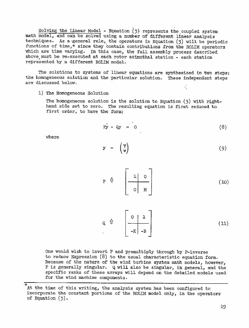
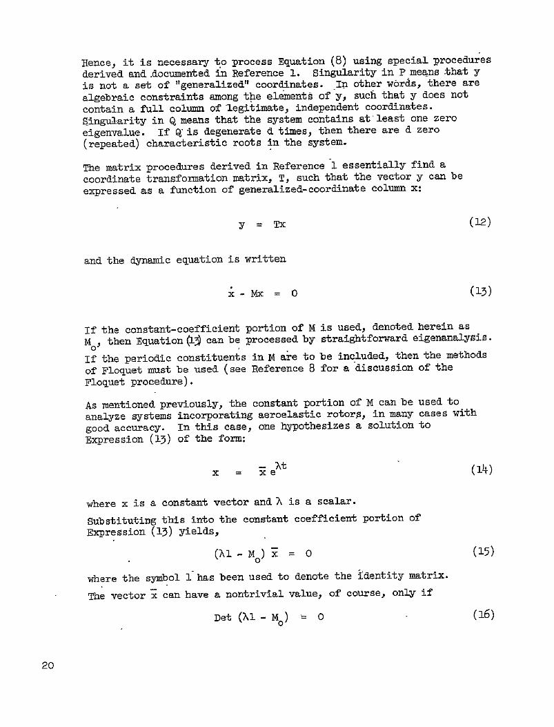
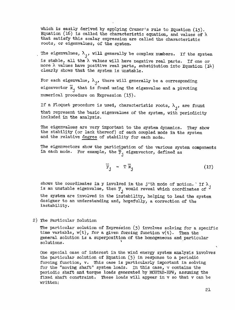
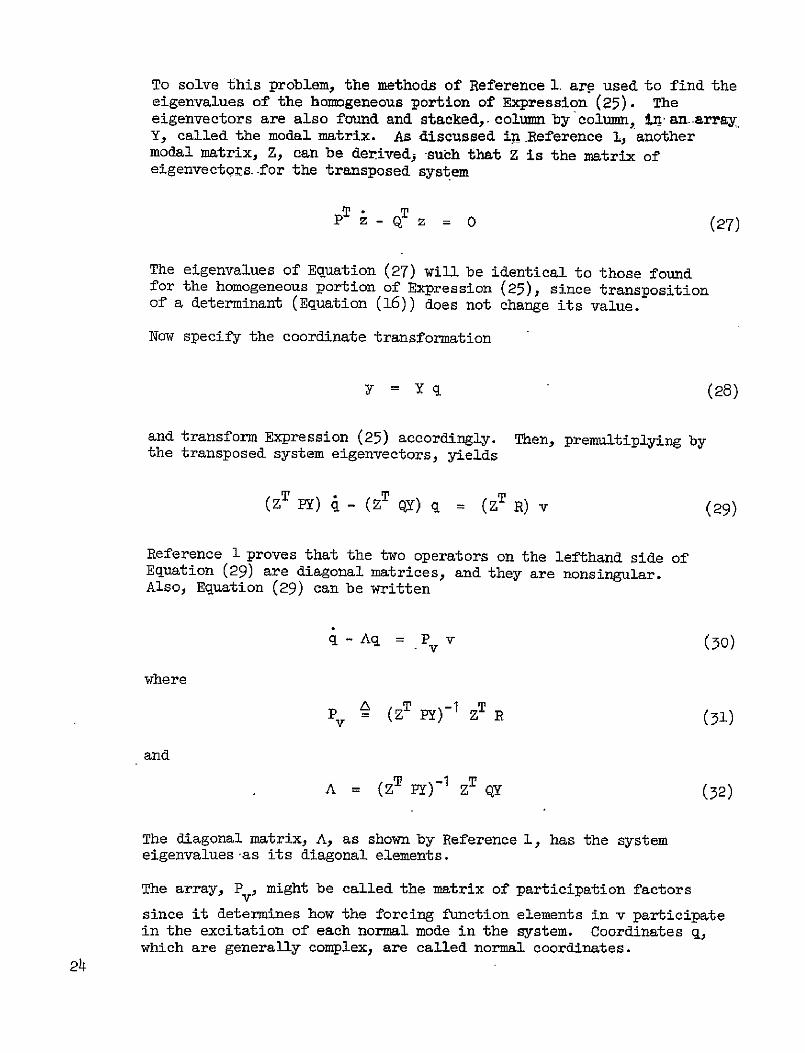
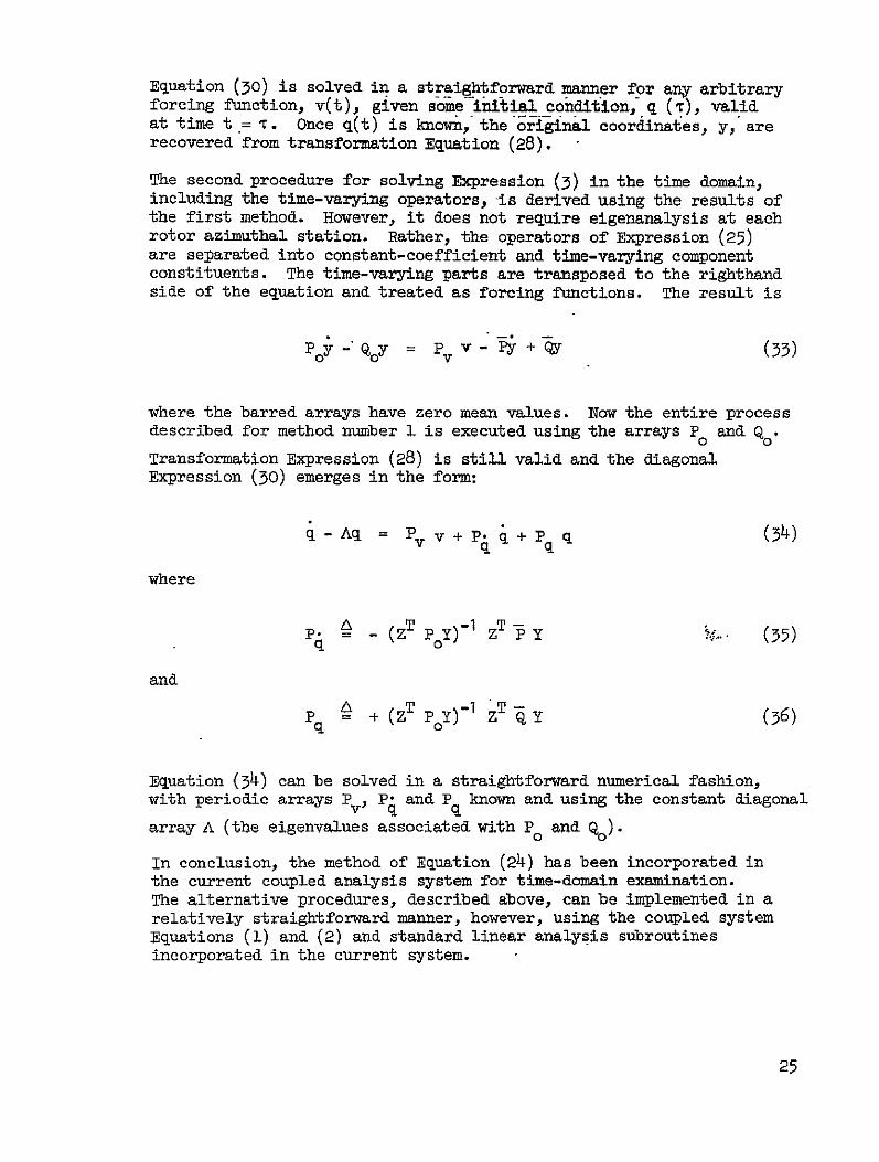
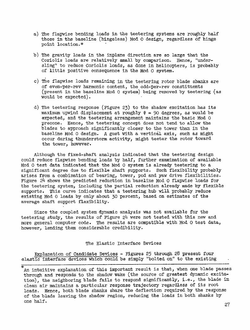
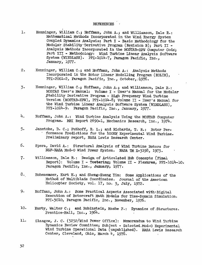
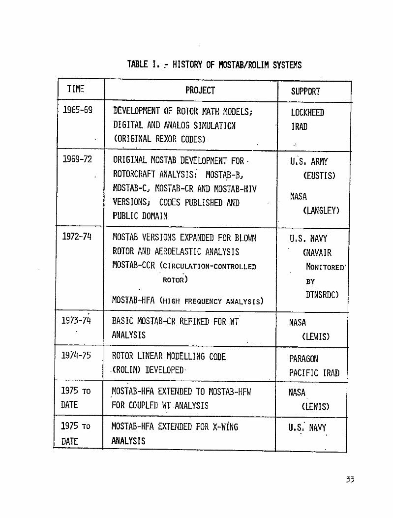
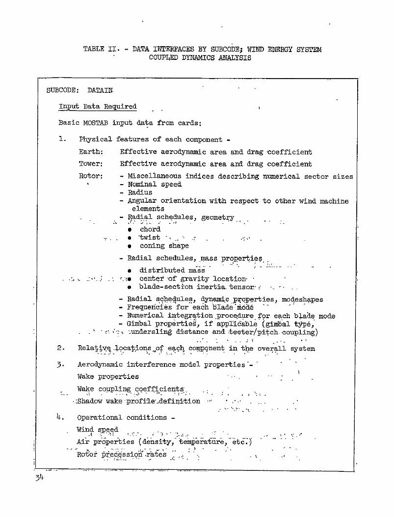

TABLE II - Continued
5 Miscellaneous numerical indices (numerical differentiation increments etc)
Output Data Produced
1 Formatted printed input data (line printer)
2 Unformatted binary data file for input to MOSTAB (sequential access disk or tape file)
SUBCODE MOSTAB-HFW
Input Data Required
1 Data file unit definition and executive option flag (card)
2 Binary file produced by subcode DATAIN (disk or tape)
Output Data Produced (Line Printer)
1 Essential constant data for rotor analysis generalized masses completed modeshape functions etc
2 Results of successive trim-search passes
3 Results of successful trim search -
Rotor average shaft loads produced for trim (resolved to a nonrotating coordinate system)
Wake velocity components (eg retardation velocities) developed at trim
Average power produced
4 Gradient arrays showing rotor shaft load responses to variations in relative wind speed components shaft precession rates and rotor control variations
Output Data Produced (PROCES File - Sequential Access Tape or Disk)
1 Rotor blade motion data at trim - blade modal coordinates and their time derivatives as a function of blade azimuth
35
TABLE II - Continued
2 Gimbal degrees of freedom motions and their time deri-vatives vs azimuth (if applicable)
3- Rotor blade internal loads vs radius and azimuth
4 Shaft loads produced by one blade vs azimuth
5 Aerodynamic distributed loads data vs radius and azimuth including angle of attack mach number dynamic pressure lift drag and moment coefficients and distributed force and moment air loads
Output Data Produced (ROLIMX File - Sequential Access Tape or Disk)
1 Basic geometric and trim-search data -
Relative geometric location of elements in wind turbine system
Mass properties of rigid body mass elements associated with system
Trim-search loads results
2 Linear math model for a single rotor blade -
Shaft loads
Gimbal error function (if applicable)
Generalized forcing function applied to blade modes
These linear math models appear as gradient arrays operating on all blade and shaft degrees of freedom and on control and rotor speed input functions and their time derivatives The gradient
arrays are functions of azimuth
3 Linear math models representing the aerodynamic couplings among the aerodynamic elements of the wind turbine system
SUBCODE PROCES
Input Data Required
1 Data file unit numbers and executive option indices (card)
2 PROCES data file produced by MOSTAB-HFW (see MOSTAB-HFW output data produded PROCES data file above)
36
TABLE II - Continued
Output Data Produced (Line Printer)
1 Formatted printout of the basic trim loads and motion data on the PROCES input data file
2 Internal blade loads and shaft loads produced by a single blade by frequency component (harmonic analysis results performed by PROCES)
Output Data Produced (Card Punch - Optional)
Harmonic blade and shaft loads
SUBCODE ROLIM
Input Data Required
1 Data file unit numbers executive option indices and harmonic and time-point specifications on ROLIM output data (card)
2 ROLIMX data file produced by MOSTAB-HFW (see Subcode MOSTAB-HFW Output Data Produced above)
Output Data Produced (Line Printer and Sequential Access Tape or Disk File)
Linear math model of rotor system including all blades aerodynamically coupled (and mechanically coupled in the case of gimballed rotor analysis)
1 Model arrays operating on rotating coordinates and expressed as a function of azimuth position
2 Same as 1 except expressed as sinecosine Fourier aoefficients
3 Same as 2 except expressed as amplitudephase angle Fourier entities
4 Model arrays transformed to operate on multi-blade coordinates shymodels have reduced one-per-rev components - expressed as functions of blade azimuth position
5 Same as 4 except expressed in sinecosine Fourier coefficients
57
TABLE II - Continued
6 Same as 5 except expressed in amplitudephase angle Fourier entities
SUBCODE COUPLED DYNAMIC SYSTEM LINEAR ANALYSIS (WINDLASS)
Input Data Required (Tape or Disk File)
Type 4 output data produced by ROLIM linear rotor math model operating on multi-blade coordinates and expressed in sinecosine coefficient form (tape or disk file)
Input Data Required (Cards)
1 Data file unit definition and executive option flags
2 Executive specification indices which define by code -
Input data items
Independent variables to be included in the coupled system dynamic equation
Dependent variables associated with the coupled system dynamic equations
Variables defined as removable ie variables included in the elemental formulations of the linear math models which are to be ultimately calculated but which can be eliminated from the basic coupled system dynamic equation
Miscellaneous other executive specification indices
3 Physical data associated with each component of the wind energy system excluding the rotor -
Tower Modeshapes frequencies and mass properties base flexibilities inertia and damping properties dimensional geometry
Power Train Inertia stiffness damping and gear ratio coefficient
associated with each building block in the power train specification indices which link the power train building blocks
38
TABLE II - Concluded
Control System (Model includes dynamic characteristics of power
machinery power machinery controls power generating reflected torques and network elements) -Loop specifications transfer functions and gains
Pod (Nacelle) - Stiffness and inertia properties geometry at rotor tower and power train interface locations
4 Harmonic coefficients required to define dynamic shaft and blade loads produced by subcode PROCES
Output Data Produced (Line Printer)
1 Linear operators in ccupled system dynamic equation
2 Linear operators in removable variable equation (solvable from results of coupled system dynamic equation)
3 Eigenvalues and eigenvectors (reflecting coupled system stability) computed from the homogeneous portion of the dynamic equation
4 Time-history responses of selected system independent and removable variables representing the coupled system perturbation responses from the trim condition responses calculated by MOSTAB-HFW
5 Time-history responses periodic blade root loads superposition of trim loads computed by MOSTAB-HFW and perturbation coupled dynamic loads
39
TABLE III - METHODS OF DYNAMIC ANALYSIS-- ROTOR SYSTEMS
ADVANTAGES DISADVANTAGES
TIME-DOMAIN SIMULATION
s MANY DOF AND NONLINEARITIES EXCESSIVE COMPUTER COSTS
CONSTANT RE-SOLUTION FLEXIBLE PROGRAMMABILITY DIFFICULT STABILITY
EVALUATIONS NUMERICAL INSTABILITY
HAZARD
FREQUENCY-DOMAIN SOLUTION STANDARD PROCEDURES
CLEAR STABILITYEVALUATION CONSTANT COEFFICIENTS REQUIRED
-e-COMPONENT MODELS QUASI-STATIC ASSUMPTION
MOSTABROLIM SYSTEM
ALL ADVANTAGES OF REQUIRES FLOQUET OR FREQUENCY-DOMAIN ROOT-PERTURBATION
STABILITY ANALYSIS - METHOD ANALYSIS LINEAR ANALYSIS
PERIODIC MATH MODELS HNIGH FREQUENCY ROTOR
MODES
4o
TABLE IV - VECTORS FOR NIND TURBINE COUPLED SYSTEM
DescriptionaSymbol
c c c Control system inputs to rotor (NC)
f Perturbation load on rotor due to freeing fixed shaft (6)
fEP External load applied to pod (mP6)
fEPR Load at podrotor interface point applied topod (6)
fEPT Load at podtower interface point due to elasticdeformation of pod (6)
(NT6)fET External loads applied to tower
fH Total load on moving hub at rotorpod interfacepoint (6)
(6)fTP Load at podtower interface point applied to tower
fo Fixed shaft load applied to hub mass - from MOSTAB-HFW(6)
f Total moving shaft load applied to hub mass (6)0
h2 b External inputs to control system (iH)
x x x Rotor shaft perturbation motion (6)
X p Pod grid point displacements (NP6)
XT xT Displacement acceleration of tower grid points (NT6)
xTr7 p Displacement icceleration of towerpod interface point (6)
y Rotor degrees of freedom (NY)
a Control system degrees of freedom (NA)
YB Power train gear box reaction torque applied to pod (NBOX)
7C Control system torque applied to power train (1)
7cp Control system torque applied to pod (NGCP)
aItems in parentheses are vector length (see Table VI)
41
TABLE IV - Concluded
Symbol Description
rEP
7RPT
sect
(Power
CRPTV cPFT
External torque applied to power train (NPHI)
Power train torque applied to rotating hub mass
Tower base degrees of freedom (5 or 6)
Tower modal coordinates (NMv)
train independent degrees of freedom (NrnI)
Rotor rotation speed and acceleration perturbations (1)
()
4j
bull j
Rotor azimuth angle (1)
Rotor speed and acceleration perturbations (1)
42
TABLE V - OPERATORS FOR WIND TURBINE COUPLED SYSTEM
Symbol Description
AUo Control system operators
B3 BEQ BNj Damping operators for power train equations
BP BRW BC
B h) Control system operators for external input h
BI B B- Y Y y
Control system operators for rotor degrees of freedom y
B B Control system operators for rotor velocity and acceleration a
D D- Relate control system degrees of freedom to rotoraYcontrol variables
ECp Rotational transformation and partitioning operator for control system torques applied to pod
EEX Rotational transformation matrices for externally applied pod loads
Rotational transformation operator for pod loads at
EpR the rotorpod interface point
EppT Rotational transformation and partitioning operator for power train gear box torques applied to pod
ETp Rotational transformation matrix to express tower loads and deflections in the pod reference system
EXp Rotational transformation and partitioning operatorPR for pod deflections at the rotorpod interface point
E Relates control system degrees of freedom to generatora torque
FT Tower modal force participation factor for external tower loads
F Tower modal force participation factor and partitioning I operator for load at towerpod interface point
43
TABLE V - Continued
Symbol Description
G
GI
Tower grid point geometric operator for exterhal tower loads Tower grid point geometry and partitioning operator
for load at towerpod interface point -
GT Tower grid point geometric operator for external tower loads
IC Partitions generator torque 7yC reaction to appropriate gear box
IEP Partitions main gear torques to power train dofs
IEPT Applies the podtower interface load to the approprpod degrees of freedom
te
IPF
PT
Partitions reactions applied by the rotor to the pod
Partitions out those pod degrees of freedom at the podtower interface point
XO Partitions fixed shaft loads fo to rotorpod interface point
I
IXT
Partitions fixed shaft torque from f to power train
Partitioning operator for motion of towerpod interface point
Partitions out the five rotor shaft displacements that ate compatible with the pod
Y I Iy
Partitioning operators for moving shaft degrees of freedom
JB JP5
J
JEQ JN
JR JqP
Inertia operators for power train equations
Effective inertia of tower base including mass
by tower
loading
JH Rotor polar moment of inertia
44
TABLE V - Continued
Symbol
JX
K
B KEQ KN Kp) KR -K (
KpPPod
KO
M
MH
Ma
M
P
P
Q RcR R
Rf
Rj
U
UB
Description
Partitioned rotor polar moment of inertia
Power train shaft torsional stiffness operator or tower base stiffness operator
Stiffness operators for power train equations
stiffness operator or power train stiffness operator Differential stiffness operator for fixed shaft load in moving hub coordinate system
Rotor acceleration operator from ROLIM
Non-spinning rotor hub mass matrix
Pod mass matrix transferred to towerpod interfacepoint
Tower grid point mass loading on tower modes
Tower modal mass loading on tower base
Rotor velocity operator from ROLIM
Relates control system response to torques on the pod
Rotor displacement operator from ROLIM ROLIM operators for applying control inputs to rotor
ROLIM operator for applied rotor shaft load
ROLIM operators for changes in rotor speed andacceleration
Unity 6 x 6 operator
Unity operator for power train gear box torquereactions
45
TABLE V - Concluded
Symbol Description
U Unity-operator for rotor controls c c and -
UCp Unity operator for control system torque reaction to pod 7 Cp
UT Unity operator for tower degrees of freedom
U Unity operator for tower modal degrees of freedom
U1 Unity I x 1 operator
W Tower modal frequency operator
X Tower mode shapes fixed base
46
TABLE VI - VECTOR LENGTHS FOR WIND TURBINE COUPLED SYSTEM
Symbol Description
NA Control system degrees of freedom
NB Tower base degrees of freedom (5 or 6)
NBOX Power train gear boxes
NC Rotor control degrees of freedom
NEV Eigenvalues in tower modal model
NGCP Interface degrees of freedom between pod and control system
NH External inputs to control system
NPHI Power train gear block elements and independent degrees of freedom
NP6 Pod degrees of freedom (6 times the number of grids)
NT6 Tower degrees of freedom (6 times the number of grids)
NY ROLIM rotor model degrees of freedom
47
TABLE VII - TEETERING HUB DESIGN CONCEPTS - WEIGHTS AND OTHER DESIGN DATA
Teetering concept
Weight a outboardShifto Hub (M
Undersling )
Stop Mechanism
Description Comments
Long Yoke 15100 -0178 0478 Hydraulic Cylinders
Long yoke places teetering axis near overall cg
Requires modified outboard hub plateheaviest concept
Short Yoke 9800 0178 -o386
Hydraulic Cylinders
Short yoke places teetering axis near shaft face for minimum weight
Negative undershysling is unconventi6nal
Linkage 10200 0381 O914 HyIdraulic Cylinders
Basic four-bar linkage places teetering axis at classical under-slung location
Least conventional teetering aais translates slightly as linkage moves
a Stop mechanism not included
TABLE VIII - BLADE ROOT FLEXURES - SUMMARY
DESIGN
Material Modulus of Elasticity (1010 Nm2 ) Dimensions (m) Flexure Weight (N blade) Total Assembly Weight (N blade) Divergence Speed msec from TE 45 degrees
Inplane Natural Frequency (per-rev at n = 4aradsec) Inplane Bending Moment Range (N - m x iO3)
2 -8 ) Maximum Flexure Inplane Stress (N x
Flapwise Natural Frequency (per-rev at a= 4aradsec) Maximum Flapwise Bending Moment (N-m x 103) Flapwise Bending Moment Reduction Maximum Flexure Flapwise Stress (Nm2 xlol
Maximum Deflection When Passing Tower (i) Deflection Increase
Zero Load Steady Conet (angle from vertical)
A B Steel Steel
Unsymmetric Symmetric
4340 Steel HT to 1lxlO9Nm2 shy21 21
074x147xl46 12 dia x 152 1748 1792 6227 6227 474 6o8
191P 1-50P +77 to -85 +81 to -119 324 69
150P 191P 515 895
67 43393 531
0 67 39 -43
4 degrees 5 degrees
C D Fiberglass Fiberglass
Unsynmetric Symmetric
Unidirectional Fiberglass 3-9 39
IOx198x91 16 dia x 91 578 578
4581 4581 456 581
191P 150P +34 to -85 +81 to -119
131 296
150P 191P 515 85
67159 221
0 o6 -4
4 degrees 5 degrees
Preliminary - Dimensional revisions (to stiffen) are required to achieve 15P lowest frequency Over IAOSTAB prediction for current Mod-O rigid shaft (Figure 4 Reference 8) Rigid Shaft Mod-O prediction is +34 to -85 N - m x 10-3 (Figure 44 Reference 8) Rigid Shaft Mod-O prediction is 07 m at = 10 degrees (Figure 45 Reference 8) t Assumes 7 degrees precone zero load steady cone for current Mod-O = 6 degrees from vertical
FIGURE 1- COUPLED DYNAMICS ANALYSIS (MOSTAS) - GLOBAL ARRANGEMENT
I DATA FILE INDICES
TRIM RESULTS S OPTION INCLUDING POWER FLAGS EXTRACTED GRADIENT ARRAYS PROCES
DATA S READ AND PRINT FILE LOADS amp MOTION
DATA FOR TRIM LOADS AND DATAIN MOSTAB-HFW 0 PERFORM HAR- MOTION DATA
READ BASIC DATA S COMPUTE CONSTANTS MONIC ANALYSIS TIME AND INPUT DATA FILE S FIND TRIM OF BLADE AND REQUENCY
VERIFYGENERATE PROCES SHAFT LOADS DOMAIN PRINT DATA DATAD DATA
OUTPUT GRADIENT P MISC DATA-ARRAYS IICONDITIONING
ROLIMX PROCEDURES
GENERATE BASIC DATA OTN REQUIRED BY ROLIMDATAROLIM A
READ HARMONIC LOAD ATAFROM PROCES PHYSICAL DATA ANALYSIS
FOR WIND TUR- U A NORMALIZE DATA LINEAR ROTORFINE CQMPO- WINDI AqqNENTS~tEXCEP1 DATAFILE FOR SOUGHT MODEL ~RO NENTS tEXCEPT ASS
COUPLED DYNAMIC SYSTEM LINEAR ANALYSIS FREQUENCYTAIGOE N RO-CONTENT GOROTOR) COMPUTE MULTIBLADES BASIC LINEAR S WIND TURBINE SYSTEM COMPONENT MATH 5 EXPAND SINGLE- COORDINATES
MODEL SPECI- MODEL BLADE DATA TOFICATION 0 LINEAR SYSTEM COUPLED DYNAMICS SFULL ROTOR INDICES EQUATION 0 COORDINATE
I EXECUTIVE S STABILITY (EIGENVALUES AND OPTION FLAGS EIGENVECTORS) RL E PRINT
COUPLED LOADS AND MOTION RESPONSE STABILITY ANALYSIS RESULTS
-ISYSTEM COMPONENT TIME-HISTORY RESP0NSES
IBLADE ROOT LOADS- TIME HISTORY RESPONSE( WITH MOVING SHAFT AND CONTROL
FIGURE 2- TIME AND FREQUENCY DOMAIN ANALYSIS METHODS
STABILITY ANALYSIS METHODS
i [ poundIL 10 -- _ 4 - - J
_ _
1 -07 --- ----shyvpi-i z v i I 10 I
TIME DOMAIN
IM
20 _I C 100 10 I I
COMPLEX AMPLITUDE PLANE 0 iA I
-10 -130RE - aft -200 -100 I -20 sect X-- - -170-0 shy
-30 - HS-21
t-lo -40 -
01 05 1 5 10 290 FREQUENCY
ROOT LOCUS PLOT BODE PLOT
FREQUENCY MIN
51
FIGURE 3- BASIC MOSTABIROLIM ANALYSIS PROCEDURES
PRINT STABILITY DERIVATIVES
PERFORMANCE ETC
OTABEECUiIE_SYSTEMF_ INPUT TRIM-SEARCH LINEAR R0 DATA __LOGIC MODELLING LI LINEAR CARDS GLOGIC - MATH
BLADE PROGRAM PROCESS SYSTEM MOTIONS AND PRINT amp ANALYZE COMPONENT LOADS BLADE LOADS amp
MATH MODELS MOTIONS
ROLIMMODELSRVS]) ROLIMPROCESSOR-MODELS V EXPAND TO MULTI-BLADE ROTOR TMIE OR FREQUENCY s INTERFERENCE COUPLINGF MULTI-BLADE COORD XFORM
FIGURE 4 - ESSENTIAL ELEMENTS OF MOSTAB MATH MODELS
EXECUTIVE SYSTEM i
offEA VELOCITIES
REQUESI FORCES AND VELOCITIES
BEaiE INTERFERENCE
ACCELERATIONS MOMENTS ACCELERATIONS VELOCITY
CONTROLS CONTROLS amp LOADS FIELD
------------------ ------- ----------shy j-
IYNMOD ( ^WASH
EXECUTIVE CODE FORCE
TYPE OF ERO ARE TIR EN AEROELASTIC I ITREECANALYSIINERERNC
7P Al~q~I VELOCITY MODELS 6 DOF WAKE
BODY LIFT WEPIMO E
AERODYNAMIC LIFTING I SI INTEGRATION I MODEL
MULTI-DOF
BODIES SURFACES WAKEMODELSWEP AEMDE
RADIAL AND BLADE
AZIMUTHAL - AEAERO INTEGRATION
-------------------- 4------ --shy MOSTAB-C I MOSTAB-HNE I---------------------4-----------------------shy
FIGURE 5- MOSTAB EXECUTIVE LOGICAL PROCEDURE
COMP E FORCES MODamp INTERFERENCEASSEMBLEREALIEA IWTR TE
VELOCITIES -
USE ESTIMATES
ASSEMBE LINEAR MODEL OF FORCE ampINTERFERENCE
SOLVE LINEAR MODEL FOR NEW-
ESTIMATES
MT MODELS
INTERFERENCE MATH
MODELS
LOAS AND E___ MOTIONS -
FINAL CALLS
NO TIMDLINEAR MATH MODELS-LOADS
MOTIONS
ROLIMX I NEAR MODEL
54
- FIGURE 6- FUNDAMENTALS OF ROTOR ANALYSIS
~BLADE
COORDINATES SHAFT REFERENCE LINE
~~ BLADEgt ilts AXES
ROTOR AXES
ATTRIBUTES
SIMPLE ROTOR ANALYSIS AEROELASTIC ANALYSIS
ONE DOF CONSTRAINED TO A USER-SPECIFIED NUMBER
MOTION PARALLEL TO SHAFT OF DOF BLADE ELEMENT MASS AND
s BLADE ELEMENT A POINT INERTIA TENSOR
MASS SIX-DOF ELEMENTAL MODEL
BOTH
STATIC AERO-STALL AND COMPRESSIBILITY
FUNCTION OR TABLE-LOOK UP
55
FIGURE 7- AEROELASTIC BLADE ANALYSIS
SINGLE BLADE MODEL ISOLATED BY SHAFT WITH PRESCRIBED MOTION
BLADE ELEMENTS MOVE INSIX DOF
MODAL MODEL TRANSFORMS BLADE MOTION TO NORMAL COORDINATES
MODEL REQUIRES INPUT
-- MODESHAPES (6DOF) -- FREQUENCIES
-- INERTIAL PROPERTIES -- NUMBER OF DOF -- INITIAL SHAPE
BLADE-MODE INITIAL CONDITIONS DETERMINED
BY ITERATIVE PROCEDURE
GIMBAL ANALYSIS USES ITERATIVE PROCEDURE
AND SINGLE-BLADE MATH MODEL
56
FIGURE 8 - GIMBAL ANALYSIS
GIVEN SHAFT AND AIR
MOTIONSCONTROL
TRANSFORMATION
SPRESCRIBED GIMBAL MOTION Ji I SPECIFIED - -
SINGLE-BLADE MODJELshy
a BLADE MOTION
GIMBAL ERROR VS AZIMUTH
ALE YSNEAR MODEL VALID AROUND SOLUTIONESA p_
gtCONDITION NO CALCULATE SHAE LOADS
LINEAR MATH MODEL GIMBAL ERRORVS GIMBAL T
AND MODAL fOFI LOADS TO REFERENCE AXESI
SOLUTION OF LINEAR MODEL REUR I FINAL BLADE MOTION F RETURN
o ZERO GIMBAL ERRORJ
s NEW PRESCRIBED GIMBAL
MOTION
57
FIGURE 9 - ADVANCED SHADOW MODEL
RADIAL
NOMINAL INTEGRATION
SEGENSIZSETO
I NAS
REDUCED
SHADOW VELOCITY SECTOR SIZE
SPECIFIED FOR EACH
REGION
i11IfIIIfIf111IIIIIi I
rp
SHADOW PROFILE SPECIFIED AS FUNCTION
OF AZIMUTH AND RADIUS - KEYED TO
TOWER DRAG-ARBITRARY PROFILE
58
FIGURE 10- MOSTAB OUTPUTS
TRIM CONDITIONS
CONTROLS
LOADS MOTIONS
WAKE
COMPREHENSIVE LOADS AND MOTIONS
0 TIME AND FREQUENCY DOMAINS
SIX DIRECTIONS AT ALL RADII
LINEAR MATH MODELS
o STABILITY AND CONTROL DERIVATIVES
-- OVERALL
-- INDIVIDUAL COMPONENTS
0 ROLIMX DATA
59
FIGURE 11 - STEPS INROLIM PROCESS
A ROLIMX PROCEDURES USE MOSTAB MODELS TO SYNTHESIZE
LINEAR OPERATIONS FOR
o BLADE GENERALIZED FORCING FUNCTIONS
o SHAFT LOADS
s WAKE VELOCITIES
AS FUNCTIONS OF
BLADE MODAL COORDINATES (SINGLE BLADE)
s SHAFT MOTIONS
CONTROLS
o AIR VELOCITIES
B SINGLE-BLADE LINEAR MODEL EXPANDED TO FULL ROTOR -
PHASE SHIFTING PROCEDURE
C ROTOR AND WAKE MODELS COMBINED WITH RIGID-BODY SHAFT EQUATIONS TO FORM ROLIM EQUATIONS
D ROLIM EQUATIONS TRANSFORMED TO MULTI-BLADE COORDINATES
E PERIODIC OPERATORS-CONVERTED TO FREQUENCY DOMAIN
6o
FIGURE 12 - THE ROTOR LINEAR MODELLING PROGRAM
ROLIM
FINAL MODEL
My+By+ KY= YC+YC+YC+YS+Y c c c 2 S2
SHAFT DOF
BLADE MODAL
DOF ALL
y = MODES INALL CONTROLSc = BLADES
OTHER AERO-
ELASTIC DOF
Qs2 ROTOR SPEED AND ACCELERATION
PERIODIC OPERATORS PRESENTED AS TIME FUNCTIONS OR
SPECTRA - MODEL GENERATED INSIX OPTIONAL CONFIG-
URATIONS INCLUDING MULTI-BLADE COORDINATES
61
FIGURE 13 - EXAMPLE ROLIM PRINTOUTS
0
s X-WING AIRCRAFT HELO MODE ROTATING COORDINATE SYSIM
SIMPLE ALRO TEST CASE JULY 196
PSI 00
300 600 900 1200 1500 1800 2100 2400 2700 3000 3300
nC( 1 1) -704s3E-01 -33000E-01 l5152E-02
-70433E-01 -33000-01 15152E-01
-704-23E-01 -33000E-01 1515E-01
-104336-01 -33000E-01 151plusmn2L-01
nt 2 1) OD( 3 1) 54183E-01 11603E-02 8t40E-01 -18242E-02 9 3 080t-01 -140704-02 59183E-01 11603L-02 8b540t-01 -1hL42b-02 93010E-0I -14070E-02 b910bL-01 11o03E-02 0tgt40E-O1 -IL32n2E-02 3(YiE-U1 -14070E-02 59183E-0 11o03E-02 8Lf40L-01 -11242E-02 93(fi06-o1 -14070E-02
ODI 4 1) OD( 59 1) 791k6E-01 1606E+00 23717E+00 71785E-01 22993E+00 -13305E+00 9126E-01 b656E+G0 23717E+O0 7178LbE-01 2i993E+00 -13305t+00 7912oE-01 1ou5bL+UO 2371h+GO 717bbb-01 229931+0 -133051+00 7Qlli-01 lbubb+00 23717E+00 717bbL-01 22993E+00 -133G5h00
ON 6i 1) 30459E02 30437t+02 30457E+02 30459E 02 30437E+U2 30457E+02 30459E+02 304371+02 30457L+02 3045YE+02 30437E+02 30457E+u2
DD( 7T 1) 15851 -02 973OOE-03 24499E-02 23245E-02 12222E-02 12635E-02 1blOE-O2 21440E-02 23375E-02 25U44E-u2 39t5E-02 39354E-02
ODI 8t 1) 21147E-O1 24bbbE-01 2b701-d 2Y9t5E-OI 2754L-01 Z673UE-01 25bb7E-01 23b52E--61 25744 E-01 29bUCjt-1 235bb-O1 1939-0I
PSI 00
300 600 900 1200 1500 1800 2100 2400 2700 3000 3300
001 9 1) 22245E-02 12 2E-02 12t3bE-02 16150E-02 21440 -02 23375E-02 25244E-02 39655E-02 39354E-02 1SR5E-02 i7300E-03 2449k-02
U)(10 1) 00(11 1) Z7ibh-01 1blhOE-02 27546-01 Z140E-02 26730E-61 23375E-U2 25bbE-ul 25844E-02 23b52L-01 39t55E-O 2574-L-01 3935E-02 29CUOE-01 158516-02 25356E-01 97fOE-03 193136L-01 24499E-C2 21147b-01 23245E-02 24656E-02 1122E-Oz 2h470F-01 126356-02
D1(12t 1) 25bblE- 23t5gE-01 25144L-01 24boOE-01 k5356E-01 1939hE-01 21147E-01 24t5LL-01 2b3702-01 27955E-01 27554E-01 26730E-01
OD(13p 1) 2Sbrth-02 39655E-02 39354E-02 15bbE-02 97300E-03 2444E-02 23245E-02 12222E-02 12635E-02 1615O-02 i440L-o
23375E-02
OPtle 11 29bbOL-01 25356-l01 19396E-01 21147L-01 24656h-01 263706-01 27955E-01 27554k-01 2673UE-O1 258t7E-01 23652E-01 25744E-01
FIGURE 14 - TOWER MATH MODEL
Yi
FLEXIBLE STRUCTURE (FIXED BASE)
z
MOVABLE BASE MODEL BAS
-7777770
z 0
LINEAR TOWER MODEL SUPERPOSITION OF
9 -MODAL MODEL OF TOWER MASS -ELASTIC
STRUCTURE WITH FIXED BASE
o RIGID BODY MODEL ON ROTARY BASE
63
FIGURE 15 -SAMPLE CONTROL SYSTEM MODEL
COLLECTIVE
PITCH CONTROL
WIND] WIND
TURBINE ROTOR MODEL
u v
V
q r--
ROTOR
DOF
----------------WINCON yi
-------------------- r
+ s + 2 ~
I
ALOITM
ALOITM
----- --
IPT - -- -
INUT
IROTOR
SSPEED a IP
Ie
64a
GiENERAL monll INERTIA
I Ii s STIFFNESS s DAMPING
s GEAR RATIO
I I
I
I I [] I
-------------------------
dega I
m-ROTOR TORQUE -- -shy-
INCREASOR r I Ij
E 3VBELTS
GEARING
FIGURE 16 - POWER TRAIN DYNAMIC MATH MODEL
FIGURE 17 WIND TURBINlE SYSTEM BLOCK DIAGRAM
-PITC CONROLMAflOELSTIC ROTOR
Aaamp E]y+BBBf11fln+Eif (C-1) State Space Model I
UccDc(C-) P-Qy- IY+Re++R+RA~+n (R-12)
1Pa (C-1) Qadnatlc Space ModelshyyW+Py44v = Eff+Ra ctc+Pfllf (R-12)
=~7C
1ka ) CR-8)
TE 9 (R-9)
lx Ix t
PNE TRAIN__ I f H tJTC=E(+ C Eifurplcc PP PPPP Mj=K0 ) XIf 0 -GTf6 1X0 f0 CR-i)
VPP C-vrfrvp ThPR - RX(R-2)D-i)
U1RTrR+R-E ip+p~~lpPp (D-2) S J+I4toUijo (R-3)
lpM=U1_ (R-4)URB~1 XT uyp ( (-) U1___________ PT_____________ Uj Rpu3i (n-5) UffI-U31 (a-10)
u RPt (n-6) UA-uii CR-fl)
KI n+mt+wX+E9 = Er~xP (Pp2)
70CP UXPR - LEXR (P-3)
TOM POD MASS
UJrIW44N = FTfET-FIfTn (Tn-1)
GjtrTG t T P I um + E TpT (P-5)
U = Xj + G5 (T-3) T J 4KS- 1 f
2 UTxT= X 9+ G9 (T-4)
uT mInxTr (T-5) = (r-6)U I~X
Q 4 4 66
FIGURE 18 - LONG YOKE TEETERING DESIGN
10 a (39 12 in)
1 8 1 2-7nL-n)
- elI
Kf- ___-
0I
i bull8 LuIj
CTCO
FIGURE 19 - SHORT YOKE TEETERING CONCEP tTBD-
V 686 m _ 051 m- (27 in) (2in)
-(19 Od Co495 n in)
1109 in (43 in)
~-(7in+ 7c 40z1 178 m
FIGURE 20 - LINKAGE TEETERING CONCEPT
_--_ r
(36-rinw
o 81 m (1 in)
FIGURE 21 - ROOT OUT-OF-PLANE MOMENT
Conditions V = 12msec 9 = -80 n= 42 radsee = 7750
150 Legend (MOSTAB-HFW)
00 Rigid Shaft No Teeter
125- -Teeter Zero Undersling
I0000-
75 -Teeter
Teeter 046m Undersling
092m Undersling
Io Test Data Reference II Figure lIla
H0 0 3
o O 360 20 I 30 33 360 -5
-25- Position Deg
-2t -2s-Azimuthal
FIGURE 22 - ROOT IN-PLANE MOMENT
40
20 20 -
0t 60 90 120 80 210 240 270 330 J0 o A
1-401
- Legend (MSTAB-mW)
-60- Rigid Shaft No T
-60-Teeter Teeter
Zero tlndereling o46m Unersling
Teeter 092m Underling
00 Test Data Reference 11 Pigure ii
-80-
Azimuthal Position Deg
FIGURE 23 - BLADE TIP DEFLECTION
125 40
075
0s
05-N
30
20
I-
Nshy
00 o n V 4 a
4 0
p
-0-25-
F
E
44
S-0-
Agimuthal oston
30 60 9020 50 802 240 Conditions V= l2nsec A = -8deg0= 42 radfsec = t750
s ________ igid Shaft No Teeter
Teeter Blade Bending Only
270 300 I
33
bull
360
Teeter Blade Bending + Hub Rotation
-20 - -shy
-075
-301
FIGURE 24 - BLADE MOMElT REDUCTION EXPECTED FROM TEETERING AS A FUNCTION OF PRESEkT HUB SUPPORT STIFFNESS
50 - shy
4o
318
30
24
S 20 i0 - - _i___e_
20 -
Range tox
Present Mod-C
0 001 005 01 02 08 10 10T t t T
Rigid twsort (120) (15) (1125)
Presnt bktio of Blad6 Sfts to popor tUffmmu 1It$ W)6
FIGURE 25 -ELASTIC INTERFACE
FLEXURE A
-SEC-T 8-LI_
0074m x 0J-47m x 14 6m long
4340 srre liT MOOO-To 5
74YCA YSZLO
7h
~FIGURE 26 -
ELASTIC INTERFACE
FLEXURE B ---SACT2CA C-Cshy
c C
COLLE-- PLIo 01m da x l52m long
73 D A I M -L
- FIGURE 27 -
ELASTIC INTERFACE
FLEXURE C - SC7YON 4- shy
ill
SPLIT CZLtET
FIBERLASS
S 39 Y 7r
BEAIMCStlppCns76
REVERSE CONING
STRAP-FOR ST ELECRIC GROUND
1O1m x 0198m x 091m long
J i
3WIECVONA9tB ISLt
FIGU= 28 -ELASTIC INTERFACE FLEXURE D
17~
O16m dia x 091m long
Ly
UNpPrOflf pr ASS
FIGURE 29 - ROOT OUT-OF-PLA14E BEDING MOMENT
175 25 Conditions V= 12msec ep -8S= 42 radsec Vs9 plusmnT Legend (MOSTAB-HFW)
50 Root Flexure Unmatched Stiffness
00- - Root Flexure Matched Stiffness
125 Mod-n Baseline Rigid Shaft
7S- Teetered Hub Zero Undersling
00 T
90 75- II
50-H75 if0251
2-I
o 00 0 A I
306 S 20 150 06- -210 240 -gt7 3M0 360
-25 -25- Azimuthal Position Deg
-50
FIGURE 30 - ROOT IN-PLANE BENDING MOMENT
00- 75 ConditionsV=12msee j = -80 9= 42 radsec$ s plusmn750
-- I ( MOSTAPHFW Results)-gend
Hoot Flexure Unmatched Stiffness75 - 50Leed--oot Flexure Matched Stiffnes
50 Mod-O Baseline Rigid Shaft
Teetered25 Hub Zero Underalinj
25 -_ - - -
IiI1 I
300~ 60 TO 720 180 20240 270 30033fl
-25 ~ 2Azimuthal Position Deg
~-s0
-00 -5shy
-12- -00
0 o
FIGURE 31 - BLADE TIP DEFLECTIO11
25
0-
0
30 -
Conditions V= 12msee a==480= 12 radsec p
Legend (I4OSTAB-HF4)
Root Flexure Urmatched Stiffness
Root Flexure Matched Stiffness
Mod-O Baseline Rigid Shaft
Teetered Hub Zero Undersling
= 750
S075-
~20
0 00
0 I 4
~0 -
H S30 90
H0 120 150 80 20 240 270 300 A0 36
- 0AzimuthalPoion g
-05 -2o
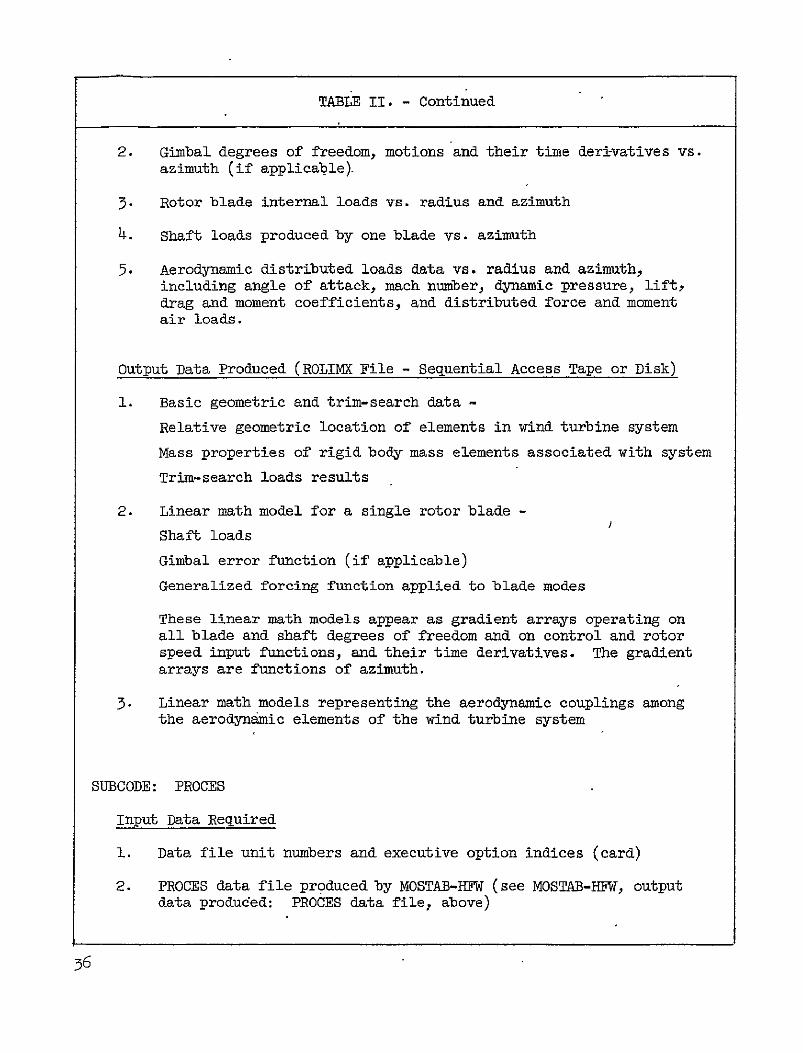
TABLE II - Continued
2 Gimbal degrees of freedom motions and their time deri-vatives vs azimuth (if applicable)
3- Rotor blade internal loads vs radius and azimuth
4 Shaft loads produced by one blade vs azimuth
5 Aerodynamic distributed loads data vs radius and azimuth including angle of attack mach number dynamic pressure lift drag and moment coefficients and distributed force and moment air loads
Output Data Produced (ROLIMX File - Sequential Access Tape or Disk)
1 Basic geometric and trim-search data -
Relative geometric location of elements in wind turbine system
Mass properties of rigid body mass elements associated with system
Trim-search loads results
2 Linear math model for a single rotor blade -
Shaft loads
Gimbal error function (if applicable)
Generalized forcing function applied to blade modes
These linear math models appear as gradient arrays operating on all blade and shaft degrees of freedom and on control and rotor speed input functions and their time derivatives The gradient
arrays are functions of azimuth
3 Linear math models representing the aerodynamic couplings among the aerodynamic elements of the wind turbine system
SUBCODE PROCES
Input Data Required
1 Data file unit numbers and executive option indices (card)
2 PROCES data file produced by MOSTAB-HFW (see MOSTAB-HFW output data produded PROCES data file above)
36
TABLE II - Continued
Output Data Produced (Line Printer)
1 Formatted printout of the basic trim loads and motion data on the PROCES input data file
2 Internal blade loads and shaft loads produced by a single blade by frequency component (harmonic analysis results performed by PROCES)
Output Data Produced (Card Punch - Optional)
Harmonic blade and shaft loads
SUBCODE ROLIM
Input Data Required
1 Data file unit numbers executive option indices and harmonic and time-point specifications on ROLIM output data (card)
2 ROLIMX data file produced by MOSTAB-HFW (see Subcode MOSTAB-HFW Output Data Produced above)
Output Data Produced (Line Printer and Sequential Access Tape or Disk File)
Linear math model of rotor system including all blades aerodynamically coupled (and mechanically coupled in the case of gimballed rotor analysis)
1 Model arrays operating on rotating coordinates and expressed as a function of azimuth position
2 Same as 1 except expressed as sinecosine Fourier aoefficients
3 Same as 2 except expressed as amplitudephase angle Fourier entities
4 Model arrays transformed to operate on multi-blade coordinates shymodels have reduced one-per-rev components - expressed as functions of blade azimuth position
5 Same as 4 except expressed in sinecosine Fourier coefficients
57
TABLE II - Continued
6 Same as 5 except expressed in amplitudephase angle Fourier entities
SUBCODE COUPLED DYNAMIC SYSTEM LINEAR ANALYSIS (WINDLASS)
Input Data Required (Tape or Disk File)
Type 4 output data produced by ROLIM linear rotor math model operating on multi-blade coordinates and expressed in sinecosine coefficient form (tape or disk file)
Input Data Required (Cards)
1 Data file unit definition and executive option flags
2 Executive specification indices which define by code -
Input data items
Independent variables to be included in the coupled system dynamic equation
Dependent variables associated with the coupled system dynamic equations
Variables defined as removable ie variables included in the elemental formulations of the linear math models which are to be ultimately calculated but which can be eliminated from the basic coupled system dynamic equation
Miscellaneous other executive specification indices
3 Physical data associated with each component of the wind energy system excluding the rotor -
Tower Modeshapes frequencies and mass properties base flexibilities inertia and damping properties dimensional geometry
Power Train Inertia stiffness damping and gear ratio coefficient
associated with each building block in the power train specification indices which link the power train building blocks
38
TABLE II - Concluded
Control System (Model includes dynamic characteristics of power
machinery power machinery controls power generating reflected torques and network elements) -Loop specifications transfer functions and gains
Pod (Nacelle) - Stiffness and inertia properties geometry at rotor tower and power train interface locations
4 Harmonic coefficients required to define dynamic shaft and blade loads produced by subcode PROCES
Output Data Produced (Line Printer)
1 Linear operators in ccupled system dynamic equation
2 Linear operators in removable variable equation (solvable from results of coupled system dynamic equation)
3 Eigenvalues and eigenvectors (reflecting coupled system stability) computed from the homogeneous portion of the dynamic equation
4 Time-history responses of selected system independent and removable variables representing the coupled system perturbation responses from the trim condition responses calculated by MOSTAB-HFW
5 Time-history responses periodic blade root loads superposition of trim loads computed by MOSTAB-HFW and perturbation coupled dynamic loads
39
TABLE III - METHODS OF DYNAMIC ANALYSIS-- ROTOR SYSTEMS
ADVANTAGES DISADVANTAGES
TIME-DOMAIN SIMULATION
s MANY DOF AND NONLINEARITIES EXCESSIVE COMPUTER COSTS
CONSTANT RE-SOLUTION FLEXIBLE PROGRAMMABILITY DIFFICULT STABILITY
EVALUATIONS NUMERICAL INSTABILITY
HAZARD
FREQUENCY-DOMAIN SOLUTION STANDARD PROCEDURES
CLEAR STABILITYEVALUATION CONSTANT COEFFICIENTS REQUIRED
-e-COMPONENT MODELS QUASI-STATIC ASSUMPTION
MOSTABROLIM SYSTEM
ALL ADVANTAGES OF REQUIRES FLOQUET OR FREQUENCY-DOMAIN ROOT-PERTURBATION
STABILITY ANALYSIS - METHOD ANALYSIS LINEAR ANALYSIS
PERIODIC MATH MODELS HNIGH FREQUENCY ROTOR
MODES
4o
TABLE IV - VECTORS FOR NIND TURBINE COUPLED SYSTEM
DescriptionaSymbol
c c c Control system inputs to rotor (NC)
f Perturbation load on rotor due to freeing fixed shaft (6)
fEP External load applied to pod (mP6)
fEPR Load at podrotor interface point applied topod (6)
fEPT Load at podtower interface point due to elasticdeformation of pod (6)
(NT6)fET External loads applied to tower
fH Total load on moving hub at rotorpod interfacepoint (6)
(6)fTP Load at podtower interface point applied to tower
fo Fixed shaft load applied to hub mass - from MOSTAB-HFW(6)
f Total moving shaft load applied to hub mass (6)0
h2 b External inputs to control system (iH)
x x x Rotor shaft perturbation motion (6)
X p Pod grid point displacements (NP6)
XT xT Displacement acceleration of tower grid points (NT6)
xTr7 p Displacement icceleration of towerpod interface point (6)
y Rotor degrees of freedom (NY)
a Control system degrees of freedom (NA)
YB Power train gear box reaction torque applied to pod (NBOX)
7C Control system torque applied to power train (1)
7cp Control system torque applied to pod (NGCP)
aItems in parentheses are vector length (see Table VI)
41
TABLE IV - Concluded
Symbol Description
rEP
7RPT
sect
(Power
CRPTV cPFT
External torque applied to power train (NPHI)
Power train torque applied to rotating hub mass
Tower base degrees of freedom (5 or 6)
Tower modal coordinates (NMv)
train independent degrees of freedom (NrnI)
Rotor rotation speed and acceleration perturbations (1)
()
4j
bull j
Rotor azimuth angle (1)
Rotor speed and acceleration perturbations (1)
42
TABLE V - OPERATORS FOR WIND TURBINE COUPLED SYSTEM
Symbol Description
AUo Control system operators
B3 BEQ BNj Damping operators for power train equations
BP BRW BC
B h) Control system operators for external input h
BI B B- Y Y y
Control system operators for rotor degrees of freedom y
B B Control system operators for rotor velocity and acceleration a
D D- Relate control system degrees of freedom to rotoraYcontrol variables
ECp Rotational transformation and partitioning operator for control system torques applied to pod
EEX Rotational transformation matrices for externally applied pod loads
Rotational transformation operator for pod loads at
EpR the rotorpod interface point
EppT Rotational transformation and partitioning operator for power train gear box torques applied to pod
ETp Rotational transformation matrix to express tower loads and deflections in the pod reference system
EXp Rotational transformation and partitioning operatorPR for pod deflections at the rotorpod interface point
E Relates control system degrees of freedom to generatora torque
FT Tower modal force participation factor for external tower loads
F Tower modal force participation factor and partitioning I operator for load at towerpod interface point
43
TABLE V - Continued
Symbol Description
G
GI
Tower grid point geometric operator for exterhal tower loads Tower grid point geometry and partitioning operator
for load at towerpod interface point -
GT Tower grid point geometric operator for external tower loads
IC Partitions generator torque 7yC reaction to appropriate gear box
IEP Partitions main gear torques to power train dofs
IEPT Applies the podtower interface load to the approprpod degrees of freedom
te
IPF
PT
Partitions reactions applied by the rotor to the pod
Partitions out those pod degrees of freedom at the podtower interface point
XO Partitions fixed shaft loads fo to rotorpod interface point
I
IXT
Partitions fixed shaft torque from f to power train
Partitioning operator for motion of towerpod interface point
Partitions out the five rotor shaft displacements that ate compatible with the pod
Y I Iy
Partitioning operators for moving shaft degrees of freedom
JB JP5
J
JEQ JN
JR JqP
Inertia operators for power train equations
Effective inertia of tower base including mass
by tower
loading
JH Rotor polar moment of inertia
44
TABLE V - Continued
Symbol
JX
K
B KEQ KN Kp) KR -K (
KpPPod
KO
M
MH
Ma
M
P
P
Q RcR R
Rf
Rj
U
UB
Description
Partitioned rotor polar moment of inertia
Power train shaft torsional stiffness operator or tower base stiffness operator
Stiffness operators for power train equations
stiffness operator or power train stiffness operator Differential stiffness operator for fixed shaft load in moving hub coordinate system
Rotor acceleration operator from ROLIM
Non-spinning rotor hub mass matrix
Pod mass matrix transferred to towerpod interfacepoint
Tower grid point mass loading on tower modes
Tower modal mass loading on tower base
Rotor velocity operator from ROLIM
Relates control system response to torques on the pod
Rotor displacement operator from ROLIM ROLIM operators for applying control inputs to rotor
ROLIM operator for applied rotor shaft load
ROLIM operators for changes in rotor speed andacceleration
Unity 6 x 6 operator
Unity operator for power train gear box torquereactions
45
TABLE V - Concluded
Symbol Description
U Unity-operator for rotor controls c c and -
UCp Unity operator for control system torque reaction to pod 7 Cp
UT Unity operator for tower degrees of freedom
U Unity operator for tower modal degrees of freedom
U1 Unity I x 1 operator
W Tower modal frequency operator
X Tower mode shapes fixed base
46
TABLE VI - VECTOR LENGTHS FOR WIND TURBINE COUPLED SYSTEM
Symbol Description
NA Control system degrees of freedom
NB Tower base degrees of freedom (5 or 6)
NBOX Power train gear boxes
NC Rotor control degrees of freedom
NEV Eigenvalues in tower modal model
NGCP Interface degrees of freedom between pod and control system
NH External inputs to control system
NPHI Power train gear block elements and independent degrees of freedom
NP6 Pod degrees of freedom (6 times the number of grids)
NT6 Tower degrees of freedom (6 times the number of grids)
NY ROLIM rotor model degrees of freedom
47
TABLE VII - TEETERING HUB DESIGN CONCEPTS - WEIGHTS AND OTHER DESIGN DATA
Teetering concept
Weight a outboardShifto Hub (M
Undersling )
Stop Mechanism
Description Comments
Long Yoke 15100 -0178 0478 Hydraulic Cylinders
Long yoke places teetering axis near overall cg
Requires modified outboard hub plateheaviest concept
Short Yoke 9800 0178 -o386
Hydraulic Cylinders
Short yoke places teetering axis near shaft face for minimum weight
Negative undershysling is unconventi6nal
Linkage 10200 0381 O914 HyIdraulic Cylinders
Basic four-bar linkage places teetering axis at classical under-slung location
Least conventional teetering aais translates slightly as linkage moves
a Stop mechanism not included
TABLE VIII - BLADE ROOT FLEXURES - SUMMARY
DESIGN
Material Modulus of Elasticity (1010 Nm2 ) Dimensions (m) Flexure Weight (N blade) Total Assembly Weight (N blade) Divergence Speed msec from TE 45 degrees
Inplane Natural Frequency (per-rev at n = 4aradsec) Inplane Bending Moment Range (N - m x iO3)
2 -8 ) Maximum Flexure Inplane Stress (N x
Flapwise Natural Frequency (per-rev at a= 4aradsec) Maximum Flapwise Bending Moment (N-m x 103) Flapwise Bending Moment Reduction Maximum Flexure Flapwise Stress (Nm2 xlol
Maximum Deflection When Passing Tower (i) Deflection Increase
Zero Load Steady Conet (angle from vertical)
A B Steel Steel
Unsymmetric Symmetric
4340 Steel HT to 1lxlO9Nm2 shy21 21
074x147xl46 12 dia x 152 1748 1792 6227 6227 474 6o8
191P 1-50P +77 to -85 +81 to -119 324 69
150P 191P 515 895
67 43393 531
0 67 39 -43
4 degrees 5 degrees
C D Fiberglass Fiberglass
Unsynmetric Symmetric
Unidirectional Fiberglass 3-9 39
IOx198x91 16 dia x 91 578 578
4581 4581 456 581
191P 150P +34 to -85 +81 to -119
131 296
150P 191P 515 85
67159 221
0 o6 -4
4 degrees 5 degrees
Preliminary - Dimensional revisions (to stiffen) are required to achieve 15P lowest frequency Over IAOSTAB prediction for current Mod-O rigid shaft (Figure 4 Reference 8) Rigid Shaft Mod-O prediction is +34 to -85 N - m x 10-3 (Figure 44 Reference 8) Rigid Shaft Mod-O prediction is 07 m at = 10 degrees (Figure 45 Reference 8) t Assumes 7 degrees precone zero load steady cone for current Mod-O = 6 degrees from vertical
FIGURE 1- COUPLED DYNAMICS ANALYSIS (MOSTAS) - GLOBAL ARRANGEMENT
I DATA FILE INDICES
TRIM RESULTS S OPTION INCLUDING POWER FLAGS EXTRACTED GRADIENT ARRAYS PROCES
DATA S READ AND PRINT FILE LOADS amp MOTION
DATA FOR TRIM LOADS AND DATAIN MOSTAB-HFW 0 PERFORM HAR- MOTION DATA
READ BASIC DATA S COMPUTE CONSTANTS MONIC ANALYSIS TIME AND INPUT DATA FILE S FIND TRIM OF BLADE AND REQUENCY
VERIFYGENERATE PROCES SHAFT LOADS DOMAIN PRINT DATA DATAD DATA
OUTPUT GRADIENT P MISC DATA-ARRAYS IICONDITIONING
ROLIMX PROCEDURES
GENERATE BASIC DATA OTN REQUIRED BY ROLIMDATAROLIM A
READ HARMONIC LOAD ATAFROM PROCES PHYSICAL DATA ANALYSIS
FOR WIND TUR- U A NORMALIZE DATA LINEAR ROTORFINE CQMPO- WINDI AqqNENTS~tEXCEP1 DATAFILE FOR SOUGHT MODEL ~RO NENTS tEXCEPT ASS
COUPLED DYNAMIC SYSTEM LINEAR ANALYSIS FREQUENCYTAIGOE N RO-CONTENT GOROTOR) COMPUTE MULTIBLADES BASIC LINEAR S WIND TURBINE SYSTEM COMPONENT MATH 5 EXPAND SINGLE- COORDINATES
MODEL SPECI- MODEL BLADE DATA TOFICATION 0 LINEAR SYSTEM COUPLED DYNAMICS SFULL ROTOR INDICES EQUATION 0 COORDINATE
I EXECUTIVE S STABILITY (EIGENVALUES AND OPTION FLAGS EIGENVECTORS) RL E PRINT
COUPLED LOADS AND MOTION RESPONSE STABILITY ANALYSIS RESULTS
-ISYSTEM COMPONENT TIME-HISTORY RESP0NSES
IBLADE ROOT LOADS- TIME HISTORY RESPONSE( WITH MOVING SHAFT AND CONTROL
FIGURE 2- TIME AND FREQUENCY DOMAIN ANALYSIS METHODS
STABILITY ANALYSIS METHODS
i [ poundIL 10 -- _ 4 - - J
_ _
1 -07 --- ----shyvpi-i z v i I 10 I
TIME DOMAIN
IM
20 _I C 100 10 I I
COMPLEX AMPLITUDE PLANE 0 iA I
-10 -130RE - aft -200 -100 I -20 sect X-- - -170-0 shy
-30 - HS-21
t-lo -40 -
01 05 1 5 10 290 FREQUENCY
ROOT LOCUS PLOT BODE PLOT
FREQUENCY MIN
51
FIGURE 3- BASIC MOSTABIROLIM ANALYSIS PROCEDURES
PRINT STABILITY DERIVATIVES
PERFORMANCE ETC
OTABEECUiIE_SYSTEMF_ INPUT TRIM-SEARCH LINEAR R0 DATA __LOGIC MODELLING LI LINEAR CARDS GLOGIC - MATH
BLADE PROGRAM PROCESS SYSTEM MOTIONS AND PRINT amp ANALYZE COMPONENT LOADS BLADE LOADS amp
MATH MODELS MOTIONS
ROLIMMODELSRVS]) ROLIMPROCESSOR-MODELS V EXPAND TO MULTI-BLADE ROTOR TMIE OR FREQUENCY s INTERFERENCE COUPLINGF MULTI-BLADE COORD XFORM
FIGURE 4 - ESSENTIAL ELEMENTS OF MOSTAB MATH MODELS
EXECUTIVE SYSTEM i
offEA VELOCITIES
REQUESI FORCES AND VELOCITIES
BEaiE INTERFERENCE
ACCELERATIONS MOMENTS ACCELERATIONS VELOCITY
CONTROLS CONTROLS amp LOADS FIELD
------------------ ------- ----------shy j-
IYNMOD ( ^WASH
EXECUTIVE CODE FORCE
TYPE OF ERO ARE TIR EN AEROELASTIC I ITREECANALYSIINERERNC
7P Al~q~I VELOCITY MODELS 6 DOF WAKE
BODY LIFT WEPIMO E
AERODYNAMIC LIFTING I SI INTEGRATION I MODEL
MULTI-DOF
BODIES SURFACES WAKEMODELSWEP AEMDE
RADIAL AND BLADE
AZIMUTHAL - AEAERO INTEGRATION
-------------------- 4------ --shy MOSTAB-C I MOSTAB-HNE I---------------------4-----------------------shy
FIGURE 5- MOSTAB EXECUTIVE LOGICAL PROCEDURE
COMP E FORCES MODamp INTERFERENCEASSEMBLEREALIEA IWTR TE
VELOCITIES -
USE ESTIMATES
ASSEMBE LINEAR MODEL OF FORCE ampINTERFERENCE
SOLVE LINEAR MODEL FOR NEW-
ESTIMATES
MT MODELS
INTERFERENCE MATH
MODELS
LOAS AND E___ MOTIONS -
FINAL CALLS
NO TIMDLINEAR MATH MODELS-LOADS
MOTIONS
ROLIMX I NEAR MODEL
54
- FIGURE 6- FUNDAMENTALS OF ROTOR ANALYSIS
~BLADE
COORDINATES SHAFT REFERENCE LINE
~~ BLADEgt ilts AXES
ROTOR AXES
ATTRIBUTES
SIMPLE ROTOR ANALYSIS AEROELASTIC ANALYSIS
ONE DOF CONSTRAINED TO A USER-SPECIFIED NUMBER
MOTION PARALLEL TO SHAFT OF DOF BLADE ELEMENT MASS AND
s BLADE ELEMENT A POINT INERTIA TENSOR
MASS SIX-DOF ELEMENTAL MODEL
BOTH
STATIC AERO-STALL AND COMPRESSIBILITY
FUNCTION OR TABLE-LOOK UP
55
FIGURE 7- AEROELASTIC BLADE ANALYSIS
SINGLE BLADE MODEL ISOLATED BY SHAFT WITH PRESCRIBED MOTION
BLADE ELEMENTS MOVE INSIX DOF
MODAL MODEL TRANSFORMS BLADE MOTION TO NORMAL COORDINATES
MODEL REQUIRES INPUT
-- MODESHAPES (6DOF) -- FREQUENCIES
-- INERTIAL PROPERTIES -- NUMBER OF DOF -- INITIAL SHAPE
BLADE-MODE INITIAL CONDITIONS DETERMINED
BY ITERATIVE PROCEDURE
GIMBAL ANALYSIS USES ITERATIVE PROCEDURE
AND SINGLE-BLADE MATH MODEL
56
FIGURE 8 - GIMBAL ANALYSIS
GIVEN SHAFT AND AIR
MOTIONSCONTROL
TRANSFORMATION
SPRESCRIBED GIMBAL MOTION Ji I SPECIFIED - -
SINGLE-BLADE MODJELshy
a BLADE MOTION
GIMBAL ERROR VS AZIMUTH
ALE YSNEAR MODEL VALID AROUND SOLUTIONESA p_
gtCONDITION NO CALCULATE SHAE LOADS
LINEAR MATH MODEL GIMBAL ERRORVS GIMBAL T
AND MODAL fOFI LOADS TO REFERENCE AXESI
SOLUTION OF LINEAR MODEL REUR I FINAL BLADE MOTION F RETURN
o ZERO GIMBAL ERRORJ
s NEW PRESCRIBED GIMBAL
MOTION
57
FIGURE 9 - ADVANCED SHADOW MODEL
RADIAL
NOMINAL INTEGRATION
SEGENSIZSETO
I NAS
REDUCED
SHADOW VELOCITY SECTOR SIZE
SPECIFIED FOR EACH
REGION
i11IfIIIfIf111IIIIIi I
rp
SHADOW PROFILE SPECIFIED AS FUNCTION
OF AZIMUTH AND RADIUS - KEYED TO
TOWER DRAG-ARBITRARY PROFILE
58
FIGURE 10- MOSTAB OUTPUTS
TRIM CONDITIONS
CONTROLS
LOADS MOTIONS
WAKE
COMPREHENSIVE LOADS AND MOTIONS
0 TIME AND FREQUENCY DOMAINS
SIX DIRECTIONS AT ALL RADII
LINEAR MATH MODELS
o STABILITY AND CONTROL DERIVATIVES
-- OVERALL
-- INDIVIDUAL COMPONENTS
0 ROLIMX DATA
59
FIGURE 11 - STEPS INROLIM PROCESS
A ROLIMX PROCEDURES USE MOSTAB MODELS TO SYNTHESIZE
LINEAR OPERATIONS FOR
o BLADE GENERALIZED FORCING FUNCTIONS
o SHAFT LOADS
s WAKE VELOCITIES
AS FUNCTIONS OF
BLADE MODAL COORDINATES (SINGLE BLADE)
s SHAFT MOTIONS
CONTROLS
o AIR VELOCITIES
B SINGLE-BLADE LINEAR MODEL EXPANDED TO FULL ROTOR -
PHASE SHIFTING PROCEDURE
C ROTOR AND WAKE MODELS COMBINED WITH RIGID-BODY SHAFT EQUATIONS TO FORM ROLIM EQUATIONS
D ROLIM EQUATIONS TRANSFORMED TO MULTI-BLADE COORDINATES
E PERIODIC OPERATORS-CONVERTED TO FREQUENCY DOMAIN
6o
FIGURE 12 - THE ROTOR LINEAR MODELLING PROGRAM
ROLIM
FINAL MODEL
My+By+ KY= YC+YC+YC+YS+Y c c c 2 S2
SHAFT DOF
BLADE MODAL
DOF ALL
y = MODES INALL CONTROLSc = BLADES
OTHER AERO-
ELASTIC DOF
Qs2 ROTOR SPEED AND ACCELERATION
PERIODIC OPERATORS PRESENTED AS TIME FUNCTIONS OR
SPECTRA - MODEL GENERATED INSIX OPTIONAL CONFIG-
URATIONS INCLUDING MULTI-BLADE COORDINATES
61
FIGURE 13 - EXAMPLE ROLIM PRINTOUTS
0
s X-WING AIRCRAFT HELO MODE ROTATING COORDINATE SYSIM
SIMPLE ALRO TEST CASE JULY 196
PSI 00
300 600 900 1200 1500 1800 2100 2400 2700 3000 3300
nC( 1 1) -704s3E-01 -33000E-01 l5152E-02
-70433E-01 -33000-01 15152E-01
-704-23E-01 -33000E-01 1515E-01
-104336-01 -33000E-01 151plusmn2L-01
nt 2 1) OD( 3 1) 54183E-01 11603E-02 8t40E-01 -18242E-02 9 3 080t-01 -140704-02 59183E-01 11603L-02 8b540t-01 -1hL42b-02 93010E-0I -14070E-02 b910bL-01 11o03E-02 0tgt40E-O1 -IL32n2E-02 3(YiE-U1 -14070E-02 59183E-0 11o03E-02 8Lf40L-01 -11242E-02 93(fi06-o1 -14070E-02
ODI 4 1) OD( 59 1) 791k6E-01 1606E+00 23717E+00 71785E-01 22993E+00 -13305E+00 9126E-01 b656E+G0 23717E+O0 7178LbE-01 2i993E+00 -13305t+00 7912oE-01 1ou5bL+UO 2371h+GO 717bbb-01 229931+0 -133051+00 7Qlli-01 lbubb+00 23717E+00 717bbL-01 22993E+00 -133G5h00
ON 6i 1) 30459E02 30437t+02 30457E+02 30459E 02 30437E+U2 30457E+02 30459E+02 304371+02 30457L+02 3045YE+02 30437E+02 30457E+u2
DD( 7T 1) 15851 -02 973OOE-03 24499E-02 23245E-02 12222E-02 12635E-02 1blOE-O2 21440E-02 23375E-02 25U44E-u2 39t5E-02 39354E-02
ODI 8t 1) 21147E-O1 24bbbE-01 2b701-d 2Y9t5E-OI 2754L-01 Z673UE-01 25bb7E-01 23b52E--61 25744 E-01 29bUCjt-1 235bb-O1 1939-0I
PSI 00
300 600 900 1200 1500 1800 2100 2400 2700 3000 3300
001 9 1) 22245E-02 12 2E-02 12t3bE-02 16150E-02 21440 -02 23375E-02 25244E-02 39655E-02 39354E-02 1SR5E-02 i7300E-03 2449k-02
U)(10 1) 00(11 1) Z7ibh-01 1blhOE-02 27546-01 Z140E-02 26730E-61 23375E-U2 25bbE-ul 25844E-02 23b52L-01 39t55E-O 2574-L-01 3935E-02 29CUOE-01 158516-02 25356E-01 97fOE-03 193136L-01 24499E-C2 21147b-01 23245E-02 24656E-02 1122E-Oz 2h470F-01 126356-02
D1(12t 1) 25bblE- 23t5gE-01 25144L-01 24boOE-01 k5356E-01 1939hE-01 21147E-01 24t5LL-01 2b3702-01 27955E-01 27554E-01 26730E-01
OD(13p 1) 2Sbrth-02 39655E-02 39354E-02 15bbE-02 97300E-03 2444E-02 23245E-02 12222E-02 12635E-02 1615O-02 i440L-o
23375E-02
OPtle 11 29bbOL-01 25356-l01 19396E-01 21147L-01 24656h-01 263706-01 27955E-01 27554k-01 2673UE-O1 258t7E-01 23652E-01 25744E-01
FIGURE 14 - TOWER MATH MODEL
Yi
FLEXIBLE STRUCTURE (FIXED BASE)
z
MOVABLE BASE MODEL BAS
-7777770
z 0
LINEAR TOWER MODEL SUPERPOSITION OF
9 -MODAL MODEL OF TOWER MASS -ELASTIC
STRUCTURE WITH FIXED BASE
o RIGID BODY MODEL ON ROTARY BASE
63
FIGURE 15 -SAMPLE CONTROL SYSTEM MODEL
COLLECTIVE
PITCH CONTROL
WIND] WIND
TURBINE ROTOR MODEL
u v
V
q r--
ROTOR
DOF
----------------WINCON yi
-------------------- r
+ s + 2 ~
I
ALOITM
ALOITM
----- --
IPT - -- -
INUT
IROTOR
SSPEED a IP
Ie
64a
GiENERAL monll INERTIA
I Ii s STIFFNESS s DAMPING
s GEAR RATIO
I I
I
I I [] I
-------------------------
dega I
m-ROTOR TORQUE -- -shy-
INCREASOR r I Ij
E 3VBELTS
GEARING
FIGURE 16 - POWER TRAIN DYNAMIC MATH MODEL
FIGURE 17 WIND TURBINlE SYSTEM BLOCK DIAGRAM
-PITC CONROLMAflOELSTIC ROTOR
Aaamp E]y+BBBf11fln+Eif (C-1) State Space Model I
UccDc(C-) P-Qy- IY+Re++R+RA~+n (R-12)
1Pa (C-1) Qadnatlc Space ModelshyyW+Py44v = Eff+Ra ctc+Pfllf (R-12)
=~7C
1ka ) CR-8)
TE 9 (R-9)
lx Ix t
PNE TRAIN__ I f H tJTC=E(+ C Eifurplcc PP PPPP Mj=K0 ) XIf 0 -GTf6 1X0 f0 CR-i)
VPP C-vrfrvp ThPR - RX(R-2)D-i)
U1RTrR+R-E ip+p~~lpPp (D-2) S J+I4toUijo (R-3)
lpM=U1_ (R-4)URB~1 XT uyp ( (-) U1___________ PT_____________ Uj Rpu3i (n-5) UffI-U31 (a-10)
u RPt (n-6) UA-uii CR-fl)
KI n+mt+wX+E9 = Er~xP (Pp2)
70CP UXPR - LEXR (P-3)
TOM POD MASS
UJrIW44N = FTfET-FIfTn (Tn-1)
GjtrTG t T P I um + E TpT (P-5)
U = Xj + G5 (T-3) T J 4KS- 1 f
2 UTxT= X 9+ G9 (T-4)
uT mInxTr (T-5) = (r-6)U I~X
Q 4 4 66
FIGURE 18 - LONG YOKE TEETERING DESIGN
10 a (39 12 in)
1 8 1 2-7nL-n)
- elI
Kf- ___-
0I
i bull8 LuIj
CTCO
FIGURE 19 - SHORT YOKE TEETERING CONCEP tTBD-
V 686 m _ 051 m- (27 in) (2in)
-(19 Od Co495 n in)
1109 in (43 in)
~-(7in+ 7c 40z1 178 m
FIGURE 20 - LINKAGE TEETERING CONCEPT
_--_ r
(36-rinw
o 81 m (1 in)
FIGURE 21 - ROOT OUT-OF-PLANE MOMENT
Conditions V = 12msec 9 = -80 n= 42 radsee = 7750
150 Legend (MOSTAB-HFW)
00 Rigid Shaft No Teeter
125- -Teeter Zero Undersling
I0000-
75 -Teeter
Teeter 046m Undersling
092m Undersling
Io Test Data Reference II Figure lIla
H0 0 3
o O 360 20 I 30 33 360 -5
-25- Position Deg
-2t -2s-Azimuthal
FIGURE 22 - ROOT IN-PLANE MOMENT
40
20 20 -
0t 60 90 120 80 210 240 270 330 J0 o A
1-401
- Legend (MSTAB-mW)
-60- Rigid Shaft No T
-60-Teeter Teeter
Zero tlndereling o46m Unersling
Teeter 092m Underling
00 Test Data Reference 11 Pigure ii
-80-
Azimuthal Position Deg
FIGURE 23 - BLADE TIP DEFLECTION
125 40
075
0s
05-N
30
20
I-
Nshy
00 o n V 4 a
4 0
p
-0-25-
F
E
44
S-0-
Agimuthal oston
30 60 9020 50 802 240 Conditions V= l2nsec A = -8deg0= 42 radfsec = t750
s ________ igid Shaft No Teeter
Teeter Blade Bending Only
270 300 I
33
bull
360
Teeter Blade Bending + Hub Rotation
-20 - -shy
-075
-301
FIGURE 24 - BLADE MOMElT REDUCTION EXPECTED FROM TEETERING AS A FUNCTION OF PRESEkT HUB SUPPORT STIFFNESS
50 - shy
4o
318
30
24
S 20 i0 - - _i___e_
20 -
Range tox
Present Mod-C
0 001 005 01 02 08 10 10T t t T
Rigid twsort (120) (15) (1125)
Presnt bktio of Blad6 Sfts to popor tUffmmu 1It$ W)6
FIGURE 25 -ELASTIC INTERFACE
FLEXURE A
-SEC-T 8-LI_
0074m x 0J-47m x 14 6m long
4340 srre liT MOOO-To 5
74YCA YSZLO
7h
~FIGURE 26 -
ELASTIC INTERFACE
FLEXURE B ---SACT2CA C-Cshy
c C
COLLE-- PLIo 01m da x l52m long
73 D A I M -L
- FIGURE 27 -
ELASTIC INTERFACE
FLEXURE C - SC7YON 4- shy
ill
SPLIT CZLtET
FIBERLASS
S 39 Y 7r
BEAIMCStlppCns76
REVERSE CONING
STRAP-FOR ST ELECRIC GROUND
1O1m x 0198m x 091m long
J i
3WIECVONA9tB ISLt
FIGU= 28 -ELASTIC INTERFACE FLEXURE D
17~
O16m dia x 091m long
Ly
UNpPrOflf pr ASS
FIGURE 29 - ROOT OUT-OF-PLA14E BEDING MOMENT
175 25 Conditions V= 12msec ep -8S= 42 radsec Vs9 plusmnT Legend (MOSTAB-HFW)
50 Root Flexure Unmatched Stiffness
00- - Root Flexure Matched Stiffness
125 Mod-n Baseline Rigid Shaft
7S- Teetered Hub Zero Undersling
00 T
90 75- II
50-H75 if0251
2-I
o 00 0 A I
306 S 20 150 06- -210 240 -gt7 3M0 360
-25 -25- Azimuthal Position Deg
-50
FIGURE 30 - ROOT IN-PLANE BENDING MOMENT
00- 75 ConditionsV=12msee j = -80 9= 42 radsec$ s plusmn750
-- I ( MOSTAPHFW Results)-gend
Hoot Flexure Unmatched Stiffness75 - 50Leed--oot Flexure Matched Stiffnes
50 Mod-O Baseline Rigid Shaft
Teetered25 Hub Zero Underalinj
25 -_ - - -
IiI1 I
300~ 60 TO 720 180 20240 270 30033fl
-25 ~ 2Azimuthal Position Deg
~-s0
-00 -5shy
-12- -00
0 o
FIGURE 31 - BLADE TIP DEFLECTIO11
25
0-
0
30 -
Conditions V= 12msee a==480= 12 radsec p
Legend (I4OSTAB-HF4)
Root Flexure Urmatched Stiffness
Root Flexure Matched Stiffness
Mod-O Baseline Rigid Shaft
Teetered Hub Zero Undersling
= 750
S075-
~20
0 00
0 I 4
~0 -
H S30 90
H0 120 150 80 20 240 270 300 A0 36
- 0AzimuthalPoion g
-05 -2o
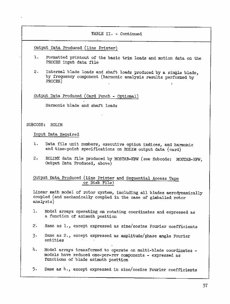
TABLE II - Continued
Output Data Produced (Line Printer)
1 Formatted printout of the basic trim loads and motion data on the PROCES input data file
2 Internal blade loads and shaft loads produced by a single blade by frequency component (harmonic analysis results performed by PROCES)
Output Data Produced (Card Punch - Optional)
Harmonic blade and shaft loads
SUBCODE ROLIM
Input Data Required
1 Data file unit numbers executive option indices and harmonic and time-point specifications on ROLIM output data (card)
2 ROLIMX data file produced by MOSTAB-HFW (see Subcode MOSTAB-HFW Output Data Produced above)
Output Data Produced (Line Printer and Sequential Access Tape or Disk File)
Linear math model of rotor system including all blades aerodynamically coupled (and mechanically coupled in the case of gimballed rotor analysis)
1 Model arrays operating on rotating coordinates and expressed as a function of azimuth position
2 Same as 1 except expressed as sinecosine Fourier aoefficients
3 Same as 2 except expressed as amplitudephase angle Fourier entities
4 Model arrays transformed to operate on multi-blade coordinates shymodels have reduced one-per-rev components - expressed as functions of blade azimuth position
5 Same as 4 except expressed in sinecosine Fourier coefficients
57
TABLE II - Continued
6 Same as 5 except expressed in amplitudephase angle Fourier entities
SUBCODE COUPLED DYNAMIC SYSTEM LINEAR ANALYSIS (WINDLASS)
Input Data Required (Tape or Disk File)
Type 4 output data produced by ROLIM linear rotor math model operating on multi-blade coordinates and expressed in sinecosine coefficient form (tape or disk file)
Input Data Required (Cards)
1 Data file unit definition and executive option flags
2 Executive specification indices which define by code -
Input data items
Independent variables to be included in the coupled system dynamic equation
Dependent variables associated with the coupled system dynamic equations
Variables defined as removable ie variables included in the elemental formulations of the linear math models which are to be ultimately calculated but which can be eliminated from the basic coupled system dynamic equation
Miscellaneous other executive specification indices
3 Physical data associated with each component of the wind energy system excluding the rotor -
Tower Modeshapes frequencies and mass properties base flexibilities inertia and damping properties dimensional geometry
Power Train Inertia stiffness damping and gear ratio coefficient
associated with each building block in the power train specification indices which link the power train building blocks
38
TABLE II - Concluded
Control System (Model includes dynamic characteristics of power
machinery power machinery controls power generating reflected torques and network elements) -Loop specifications transfer functions and gains
Pod (Nacelle) - Stiffness and inertia properties geometry at rotor tower and power train interface locations
4 Harmonic coefficients required to define dynamic shaft and blade loads produced by subcode PROCES
Output Data Produced (Line Printer)
1 Linear operators in ccupled system dynamic equation
2 Linear operators in removable variable equation (solvable from results of coupled system dynamic equation)
3 Eigenvalues and eigenvectors (reflecting coupled system stability) computed from the homogeneous portion of the dynamic equation
4 Time-history responses of selected system independent and removable variables representing the coupled system perturbation responses from the trim condition responses calculated by MOSTAB-HFW
5 Time-history responses periodic blade root loads superposition of trim loads computed by MOSTAB-HFW and perturbation coupled dynamic loads
39
TABLE III - METHODS OF DYNAMIC ANALYSIS-- ROTOR SYSTEMS
ADVANTAGES DISADVANTAGES
TIME-DOMAIN SIMULATION
s MANY DOF AND NONLINEARITIES EXCESSIVE COMPUTER COSTS
CONSTANT RE-SOLUTION FLEXIBLE PROGRAMMABILITY DIFFICULT STABILITY
EVALUATIONS NUMERICAL INSTABILITY
HAZARD
FREQUENCY-DOMAIN SOLUTION STANDARD PROCEDURES
CLEAR STABILITYEVALUATION CONSTANT COEFFICIENTS REQUIRED
-e-COMPONENT MODELS QUASI-STATIC ASSUMPTION
MOSTABROLIM SYSTEM
ALL ADVANTAGES OF REQUIRES FLOQUET OR FREQUENCY-DOMAIN ROOT-PERTURBATION
STABILITY ANALYSIS - METHOD ANALYSIS LINEAR ANALYSIS
PERIODIC MATH MODELS HNIGH FREQUENCY ROTOR
MODES
4o
TABLE IV - VECTORS FOR NIND TURBINE COUPLED SYSTEM
DescriptionaSymbol
c c c Control system inputs to rotor (NC)
f Perturbation load on rotor due to freeing fixed shaft (6)
fEP External load applied to pod (mP6)
fEPR Load at podrotor interface point applied topod (6)
fEPT Load at podtower interface point due to elasticdeformation of pod (6)
(NT6)fET External loads applied to tower
fH Total load on moving hub at rotorpod interfacepoint (6)
(6)fTP Load at podtower interface point applied to tower
fo Fixed shaft load applied to hub mass - from MOSTAB-HFW(6)
f Total moving shaft load applied to hub mass (6)0
h2 b External inputs to control system (iH)
x x x Rotor shaft perturbation motion (6)
X p Pod grid point displacements (NP6)
XT xT Displacement acceleration of tower grid points (NT6)
xTr7 p Displacement icceleration of towerpod interface point (6)
y Rotor degrees of freedom (NY)
a Control system degrees of freedom (NA)
YB Power train gear box reaction torque applied to pod (NBOX)
7C Control system torque applied to power train (1)
7cp Control system torque applied to pod (NGCP)
aItems in parentheses are vector length (see Table VI)
41
TABLE IV - Concluded
Symbol Description
rEP
7RPT
sect
(Power
CRPTV cPFT
External torque applied to power train (NPHI)
Power train torque applied to rotating hub mass
Tower base degrees of freedom (5 or 6)
Tower modal coordinates (NMv)
train independent degrees of freedom (NrnI)
Rotor rotation speed and acceleration perturbations (1)
()
4j
bull j
Rotor azimuth angle (1)
Rotor speed and acceleration perturbations (1)
42
TABLE V - OPERATORS FOR WIND TURBINE COUPLED SYSTEM
Symbol Description
AUo Control system operators
B3 BEQ BNj Damping operators for power train equations
BP BRW BC
B h) Control system operators for external input h
BI B B- Y Y y
Control system operators for rotor degrees of freedom y
B B Control system operators for rotor velocity and acceleration a
D D- Relate control system degrees of freedom to rotoraYcontrol variables
ECp Rotational transformation and partitioning operator for control system torques applied to pod
EEX Rotational transformation matrices for externally applied pod loads
Rotational transformation operator for pod loads at
EpR the rotorpod interface point
EppT Rotational transformation and partitioning operator for power train gear box torques applied to pod
ETp Rotational transformation matrix to express tower loads and deflections in the pod reference system
EXp Rotational transformation and partitioning operatorPR for pod deflections at the rotorpod interface point
E Relates control system degrees of freedom to generatora torque
FT Tower modal force participation factor for external tower loads
F Tower modal force participation factor and partitioning I operator for load at towerpod interface point
43
TABLE V - Continued
Symbol Description
G
GI
Tower grid point geometric operator for exterhal tower loads Tower grid point geometry and partitioning operator
for load at towerpod interface point -
GT Tower grid point geometric operator for external tower loads
IC Partitions generator torque 7yC reaction to appropriate gear box
IEP Partitions main gear torques to power train dofs
IEPT Applies the podtower interface load to the approprpod degrees of freedom
te
IPF
PT
Partitions reactions applied by the rotor to the pod
Partitions out those pod degrees of freedom at the podtower interface point
XO Partitions fixed shaft loads fo to rotorpod interface point
I
IXT
Partitions fixed shaft torque from f to power train
Partitioning operator for motion of towerpod interface point
Partitions out the five rotor shaft displacements that ate compatible with the pod
Y I Iy
Partitioning operators for moving shaft degrees of freedom
JB JP5
J
JEQ JN
JR JqP
Inertia operators for power train equations
Effective inertia of tower base including mass
by tower
loading
JH Rotor polar moment of inertia
44
TABLE V - Continued
Symbol
JX
K
B KEQ KN Kp) KR -K (
KpPPod
KO
M
MH
Ma
M
P
P
Q RcR R
Rf
Rj
U
UB
Description
Partitioned rotor polar moment of inertia
Power train shaft torsional stiffness operator or tower base stiffness operator
Stiffness operators for power train equations
stiffness operator or power train stiffness operator Differential stiffness operator for fixed shaft load in moving hub coordinate system
Rotor acceleration operator from ROLIM
Non-spinning rotor hub mass matrix
Pod mass matrix transferred to towerpod interfacepoint
Tower grid point mass loading on tower modes
Tower modal mass loading on tower base
Rotor velocity operator from ROLIM
Relates control system response to torques on the pod
Rotor displacement operator from ROLIM ROLIM operators for applying control inputs to rotor
ROLIM operator for applied rotor shaft load
ROLIM operators for changes in rotor speed andacceleration
Unity 6 x 6 operator
Unity operator for power train gear box torquereactions
45
TABLE V - Concluded
Symbol Description
U Unity-operator for rotor controls c c and -
UCp Unity operator for control system torque reaction to pod 7 Cp
UT Unity operator for tower degrees of freedom
U Unity operator for tower modal degrees of freedom
U1 Unity I x 1 operator
W Tower modal frequency operator
X Tower mode shapes fixed base
46
TABLE VI - VECTOR LENGTHS FOR WIND TURBINE COUPLED SYSTEM
Symbol Description
NA Control system degrees of freedom
NB Tower base degrees of freedom (5 or 6)
NBOX Power train gear boxes
NC Rotor control degrees of freedom
NEV Eigenvalues in tower modal model
NGCP Interface degrees of freedom between pod and control system
NH External inputs to control system
NPHI Power train gear block elements and independent degrees of freedom
NP6 Pod degrees of freedom (6 times the number of grids)
NT6 Tower degrees of freedom (6 times the number of grids)
NY ROLIM rotor model degrees of freedom
47
TABLE VII - TEETERING HUB DESIGN CONCEPTS - WEIGHTS AND OTHER DESIGN DATA
Teetering concept
Weight a outboardShifto Hub (M
Undersling )
Stop Mechanism
Description Comments
Long Yoke 15100 -0178 0478 Hydraulic Cylinders
Long yoke places teetering axis near overall cg
Requires modified outboard hub plateheaviest concept
Short Yoke 9800 0178 -o386
Hydraulic Cylinders
Short yoke places teetering axis near shaft face for minimum weight
Negative undershysling is unconventi6nal
Linkage 10200 0381 O914 HyIdraulic Cylinders
Basic four-bar linkage places teetering axis at classical under-slung location
Least conventional teetering aais translates slightly as linkage moves
a Stop mechanism not included
TABLE VIII - BLADE ROOT FLEXURES - SUMMARY
DESIGN
Material Modulus of Elasticity (1010 Nm2 ) Dimensions (m) Flexure Weight (N blade) Total Assembly Weight (N blade) Divergence Speed msec from TE 45 degrees
Inplane Natural Frequency (per-rev at n = 4aradsec) Inplane Bending Moment Range (N - m x iO3)
2 -8 ) Maximum Flexure Inplane Stress (N x
Flapwise Natural Frequency (per-rev at a= 4aradsec) Maximum Flapwise Bending Moment (N-m x 103) Flapwise Bending Moment Reduction Maximum Flexure Flapwise Stress (Nm2 xlol
Maximum Deflection When Passing Tower (i) Deflection Increase
Zero Load Steady Conet (angle from vertical)
A B Steel Steel
Unsymmetric Symmetric
4340 Steel HT to 1lxlO9Nm2 shy21 21
074x147xl46 12 dia x 152 1748 1792 6227 6227 474 6o8
191P 1-50P +77 to -85 +81 to -119 324 69
150P 191P 515 895
67 43393 531
0 67 39 -43
4 degrees 5 degrees
C D Fiberglass Fiberglass
Unsynmetric Symmetric
Unidirectional Fiberglass 3-9 39
IOx198x91 16 dia x 91 578 578
4581 4581 456 581
191P 150P +34 to -85 +81 to -119
131 296
150P 191P 515 85
67159 221
0 o6 -4
4 degrees 5 degrees
Preliminary - Dimensional revisions (to stiffen) are required to achieve 15P lowest frequency Over IAOSTAB prediction for current Mod-O rigid shaft (Figure 4 Reference 8) Rigid Shaft Mod-O prediction is +34 to -85 N - m x 10-3 (Figure 44 Reference 8) Rigid Shaft Mod-O prediction is 07 m at = 10 degrees (Figure 45 Reference 8) t Assumes 7 degrees precone zero load steady cone for current Mod-O = 6 degrees from vertical
FIGURE 1- COUPLED DYNAMICS ANALYSIS (MOSTAS) - GLOBAL ARRANGEMENT
I DATA FILE INDICES
TRIM RESULTS S OPTION INCLUDING POWER FLAGS EXTRACTED GRADIENT ARRAYS PROCES
DATA S READ AND PRINT FILE LOADS amp MOTION
DATA FOR TRIM LOADS AND DATAIN MOSTAB-HFW 0 PERFORM HAR- MOTION DATA
READ BASIC DATA S COMPUTE CONSTANTS MONIC ANALYSIS TIME AND INPUT DATA FILE S FIND TRIM OF BLADE AND REQUENCY
VERIFYGENERATE PROCES SHAFT LOADS DOMAIN PRINT DATA DATAD DATA
OUTPUT GRADIENT P MISC DATA-ARRAYS IICONDITIONING
ROLIMX PROCEDURES
GENERATE BASIC DATA OTN REQUIRED BY ROLIMDATAROLIM A
READ HARMONIC LOAD ATAFROM PROCES PHYSICAL DATA ANALYSIS
FOR WIND TUR- U A NORMALIZE DATA LINEAR ROTORFINE CQMPO- WINDI AqqNENTS~tEXCEP1 DATAFILE FOR SOUGHT MODEL ~RO NENTS tEXCEPT ASS
COUPLED DYNAMIC SYSTEM LINEAR ANALYSIS FREQUENCYTAIGOE N RO-CONTENT GOROTOR) COMPUTE MULTIBLADES BASIC LINEAR S WIND TURBINE SYSTEM COMPONENT MATH 5 EXPAND SINGLE- COORDINATES
MODEL SPECI- MODEL BLADE DATA TOFICATION 0 LINEAR SYSTEM COUPLED DYNAMICS SFULL ROTOR INDICES EQUATION 0 COORDINATE
I EXECUTIVE S STABILITY (EIGENVALUES AND OPTION FLAGS EIGENVECTORS) RL E PRINT
COUPLED LOADS AND MOTION RESPONSE STABILITY ANALYSIS RESULTS
-ISYSTEM COMPONENT TIME-HISTORY RESP0NSES
IBLADE ROOT LOADS- TIME HISTORY RESPONSE( WITH MOVING SHAFT AND CONTROL
FIGURE 2- TIME AND FREQUENCY DOMAIN ANALYSIS METHODS
STABILITY ANALYSIS METHODS
i [ poundIL 10 -- _ 4 - - J
_ _
1 -07 --- ----shyvpi-i z v i I 10 I
TIME DOMAIN
IM
20 _I C 100 10 I I
COMPLEX AMPLITUDE PLANE 0 iA I
-10 -130RE - aft -200 -100 I -20 sect X-- - -170-0 shy
-30 - HS-21
t-lo -40 -
01 05 1 5 10 290 FREQUENCY
ROOT LOCUS PLOT BODE PLOT
FREQUENCY MIN
51
FIGURE 3- BASIC MOSTABIROLIM ANALYSIS PROCEDURES
PRINT STABILITY DERIVATIVES
PERFORMANCE ETC
OTABEECUiIE_SYSTEMF_ INPUT TRIM-SEARCH LINEAR R0 DATA __LOGIC MODELLING LI LINEAR CARDS GLOGIC - MATH
BLADE PROGRAM PROCESS SYSTEM MOTIONS AND PRINT amp ANALYZE COMPONENT LOADS BLADE LOADS amp
MATH MODELS MOTIONS
ROLIMMODELSRVS]) ROLIMPROCESSOR-MODELS V EXPAND TO MULTI-BLADE ROTOR TMIE OR FREQUENCY s INTERFERENCE COUPLINGF MULTI-BLADE COORD XFORM
FIGURE 4 - ESSENTIAL ELEMENTS OF MOSTAB MATH MODELS
EXECUTIVE SYSTEM i
offEA VELOCITIES
REQUESI FORCES AND VELOCITIES
BEaiE INTERFERENCE
ACCELERATIONS MOMENTS ACCELERATIONS VELOCITY
CONTROLS CONTROLS amp LOADS FIELD
------------------ ------- ----------shy j-
IYNMOD ( ^WASH
EXECUTIVE CODE FORCE
TYPE OF ERO ARE TIR EN AEROELASTIC I ITREECANALYSIINERERNC
7P Al~q~I VELOCITY MODELS 6 DOF WAKE
BODY LIFT WEPIMO E
AERODYNAMIC LIFTING I SI INTEGRATION I MODEL
MULTI-DOF
BODIES SURFACES WAKEMODELSWEP AEMDE
RADIAL AND BLADE
AZIMUTHAL - AEAERO INTEGRATION
-------------------- 4------ --shy MOSTAB-C I MOSTAB-HNE I---------------------4-----------------------shy
FIGURE 5- MOSTAB EXECUTIVE LOGICAL PROCEDURE
COMP E FORCES MODamp INTERFERENCEASSEMBLEREALIEA IWTR TE
VELOCITIES -
USE ESTIMATES
ASSEMBE LINEAR MODEL OF FORCE ampINTERFERENCE
SOLVE LINEAR MODEL FOR NEW-
ESTIMATES
MT MODELS
INTERFERENCE MATH
MODELS
LOAS AND E___ MOTIONS -
FINAL CALLS
NO TIMDLINEAR MATH MODELS-LOADS
MOTIONS
ROLIMX I NEAR MODEL
54
- FIGURE 6- FUNDAMENTALS OF ROTOR ANALYSIS
~BLADE
COORDINATES SHAFT REFERENCE LINE
~~ BLADEgt ilts AXES
ROTOR AXES
ATTRIBUTES
SIMPLE ROTOR ANALYSIS AEROELASTIC ANALYSIS
ONE DOF CONSTRAINED TO A USER-SPECIFIED NUMBER
MOTION PARALLEL TO SHAFT OF DOF BLADE ELEMENT MASS AND
s BLADE ELEMENT A POINT INERTIA TENSOR
MASS SIX-DOF ELEMENTAL MODEL
BOTH
STATIC AERO-STALL AND COMPRESSIBILITY
FUNCTION OR TABLE-LOOK UP
55
FIGURE 7- AEROELASTIC BLADE ANALYSIS
SINGLE BLADE MODEL ISOLATED BY SHAFT WITH PRESCRIBED MOTION
BLADE ELEMENTS MOVE INSIX DOF
MODAL MODEL TRANSFORMS BLADE MOTION TO NORMAL COORDINATES
MODEL REQUIRES INPUT
-- MODESHAPES (6DOF) -- FREQUENCIES
-- INERTIAL PROPERTIES -- NUMBER OF DOF -- INITIAL SHAPE
BLADE-MODE INITIAL CONDITIONS DETERMINED
BY ITERATIVE PROCEDURE
GIMBAL ANALYSIS USES ITERATIVE PROCEDURE
AND SINGLE-BLADE MATH MODEL
56
FIGURE 8 - GIMBAL ANALYSIS
GIVEN SHAFT AND AIR
MOTIONSCONTROL
TRANSFORMATION
SPRESCRIBED GIMBAL MOTION Ji I SPECIFIED - -
SINGLE-BLADE MODJELshy
a BLADE MOTION
GIMBAL ERROR VS AZIMUTH
ALE YSNEAR MODEL VALID AROUND SOLUTIONESA p_
gtCONDITION NO CALCULATE SHAE LOADS
LINEAR MATH MODEL GIMBAL ERRORVS GIMBAL T
AND MODAL fOFI LOADS TO REFERENCE AXESI
SOLUTION OF LINEAR MODEL REUR I FINAL BLADE MOTION F RETURN
o ZERO GIMBAL ERRORJ
s NEW PRESCRIBED GIMBAL
MOTION
57
FIGURE 9 - ADVANCED SHADOW MODEL
RADIAL
NOMINAL INTEGRATION
SEGENSIZSETO
I NAS
REDUCED
SHADOW VELOCITY SECTOR SIZE
SPECIFIED FOR EACH
REGION
i11IfIIIfIf111IIIIIi I
rp
SHADOW PROFILE SPECIFIED AS FUNCTION
OF AZIMUTH AND RADIUS - KEYED TO
TOWER DRAG-ARBITRARY PROFILE
58
FIGURE 10- MOSTAB OUTPUTS
TRIM CONDITIONS
CONTROLS
LOADS MOTIONS
WAKE
COMPREHENSIVE LOADS AND MOTIONS
0 TIME AND FREQUENCY DOMAINS
SIX DIRECTIONS AT ALL RADII
LINEAR MATH MODELS
o STABILITY AND CONTROL DERIVATIVES
-- OVERALL
-- INDIVIDUAL COMPONENTS
0 ROLIMX DATA
59
FIGURE 11 - STEPS INROLIM PROCESS
A ROLIMX PROCEDURES USE MOSTAB MODELS TO SYNTHESIZE
LINEAR OPERATIONS FOR
o BLADE GENERALIZED FORCING FUNCTIONS
o SHAFT LOADS
s WAKE VELOCITIES
AS FUNCTIONS OF
BLADE MODAL COORDINATES (SINGLE BLADE)
s SHAFT MOTIONS
CONTROLS
o AIR VELOCITIES
B SINGLE-BLADE LINEAR MODEL EXPANDED TO FULL ROTOR -
PHASE SHIFTING PROCEDURE
C ROTOR AND WAKE MODELS COMBINED WITH RIGID-BODY SHAFT EQUATIONS TO FORM ROLIM EQUATIONS
D ROLIM EQUATIONS TRANSFORMED TO MULTI-BLADE COORDINATES
E PERIODIC OPERATORS-CONVERTED TO FREQUENCY DOMAIN
6o
FIGURE 12 - THE ROTOR LINEAR MODELLING PROGRAM
ROLIM
FINAL MODEL
My+By+ KY= YC+YC+YC+YS+Y c c c 2 S2
SHAFT DOF
BLADE MODAL
DOF ALL
y = MODES INALL CONTROLSc = BLADES
OTHER AERO-
ELASTIC DOF
Qs2 ROTOR SPEED AND ACCELERATION
PERIODIC OPERATORS PRESENTED AS TIME FUNCTIONS OR
SPECTRA - MODEL GENERATED INSIX OPTIONAL CONFIG-
URATIONS INCLUDING MULTI-BLADE COORDINATES
61
FIGURE 13 - EXAMPLE ROLIM PRINTOUTS
0
s X-WING AIRCRAFT HELO MODE ROTATING COORDINATE SYSIM
SIMPLE ALRO TEST CASE JULY 196
PSI 00
300 600 900 1200 1500 1800 2100 2400 2700 3000 3300
nC( 1 1) -704s3E-01 -33000E-01 l5152E-02
-70433E-01 -33000-01 15152E-01
-704-23E-01 -33000E-01 1515E-01
-104336-01 -33000E-01 151plusmn2L-01
nt 2 1) OD( 3 1) 54183E-01 11603E-02 8t40E-01 -18242E-02 9 3 080t-01 -140704-02 59183E-01 11603L-02 8b540t-01 -1hL42b-02 93010E-0I -14070E-02 b910bL-01 11o03E-02 0tgt40E-O1 -IL32n2E-02 3(YiE-U1 -14070E-02 59183E-0 11o03E-02 8Lf40L-01 -11242E-02 93(fi06-o1 -14070E-02
ODI 4 1) OD( 59 1) 791k6E-01 1606E+00 23717E+00 71785E-01 22993E+00 -13305E+00 9126E-01 b656E+G0 23717E+O0 7178LbE-01 2i993E+00 -13305t+00 7912oE-01 1ou5bL+UO 2371h+GO 717bbb-01 229931+0 -133051+00 7Qlli-01 lbubb+00 23717E+00 717bbL-01 22993E+00 -133G5h00
ON 6i 1) 30459E02 30437t+02 30457E+02 30459E 02 30437E+U2 30457E+02 30459E+02 304371+02 30457L+02 3045YE+02 30437E+02 30457E+u2
DD( 7T 1) 15851 -02 973OOE-03 24499E-02 23245E-02 12222E-02 12635E-02 1blOE-O2 21440E-02 23375E-02 25U44E-u2 39t5E-02 39354E-02
ODI 8t 1) 21147E-O1 24bbbE-01 2b701-d 2Y9t5E-OI 2754L-01 Z673UE-01 25bb7E-01 23b52E--61 25744 E-01 29bUCjt-1 235bb-O1 1939-0I
PSI 00
300 600 900 1200 1500 1800 2100 2400 2700 3000 3300
001 9 1) 22245E-02 12 2E-02 12t3bE-02 16150E-02 21440 -02 23375E-02 25244E-02 39655E-02 39354E-02 1SR5E-02 i7300E-03 2449k-02
U)(10 1) 00(11 1) Z7ibh-01 1blhOE-02 27546-01 Z140E-02 26730E-61 23375E-U2 25bbE-ul 25844E-02 23b52L-01 39t55E-O 2574-L-01 3935E-02 29CUOE-01 158516-02 25356E-01 97fOE-03 193136L-01 24499E-C2 21147b-01 23245E-02 24656E-02 1122E-Oz 2h470F-01 126356-02
D1(12t 1) 25bblE- 23t5gE-01 25144L-01 24boOE-01 k5356E-01 1939hE-01 21147E-01 24t5LL-01 2b3702-01 27955E-01 27554E-01 26730E-01
OD(13p 1) 2Sbrth-02 39655E-02 39354E-02 15bbE-02 97300E-03 2444E-02 23245E-02 12222E-02 12635E-02 1615O-02 i440L-o
23375E-02
OPtle 11 29bbOL-01 25356-l01 19396E-01 21147L-01 24656h-01 263706-01 27955E-01 27554k-01 2673UE-O1 258t7E-01 23652E-01 25744E-01
FIGURE 14 - TOWER MATH MODEL
Yi
FLEXIBLE STRUCTURE (FIXED BASE)
z
MOVABLE BASE MODEL BAS
-7777770
z 0
LINEAR TOWER MODEL SUPERPOSITION OF
9 -MODAL MODEL OF TOWER MASS -ELASTIC
STRUCTURE WITH FIXED BASE
o RIGID BODY MODEL ON ROTARY BASE
63
FIGURE 15 -SAMPLE CONTROL SYSTEM MODEL
COLLECTIVE
PITCH CONTROL
WIND] WIND
TURBINE ROTOR MODEL
u v
V
q r--
ROTOR
DOF
----------------WINCON yi
-------------------- r
+ s + 2 ~
I
ALOITM
ALOITM
----- --
IPT - -- -
INUT
IROTOR
SSPEED a IP
Ie
64a
GiENERAL monll INERTIA
I Ii s STIFFNESS s DAMPING
s GEAR RATIO
I I
I
I I [] I
-------------------------
dega I
m-ROTOR TORQUE -- -shy-
INCREASOR r I Ij
E 3VBELTS
GEARING
FIGURE 16 - POWER TRAIN DYNAMIC MATH MODEL
FIGURE 17 WIND TURBINlE SYSTEM BLOCK DIAGRAM
-PITC CONROLMAflOELSTIC ROTOR
Aaamp E]y+BBBf11fln+Eif (C-1) State Space Model I
UccDc(C-) P-Qy- IY+Re++R+RA~+n (R-12)
1Pa (C-1) Qadnatlc Space ModelshyyW+Py44v = Eff+Ra ctc+Pfllf (R-12)
=~7C
1ka ) CR-8)
TE 9 (R-9)
lx Ix t
PNE TRAIN__ I f H tJTC=E(+ C Eifurplcc PP PPPP Mj=K0 ) XIf 0 -GTf6 1X0 f0 CR-i)
VPP C-vrfrvp ThPR - RX(R-2)D-i)
U1RTrR+R-E ip+p~~lpPp (D-2) S J+I4toUijo (R-3)
lpM=U1_ (R-4)URB~1 XT uyp ( (-) U1___________ PT_____________ Uj Rpu3i (n-5) UffI-U31 (a-10)
u RPt (n-6) UA-uii CR-fl)
KI n+mt+wX+E9 = Er~xP (Pp2)
70CP UXPR - LEXR (P-3)
TOM POD MASS
UJrIW44N = FTfET-FIfTn (Tn-1)
GjtrTG t T P I um + E TpT (P-5)
U = Xj + G5 (T-3) T J 4KS- 1 f
2 UTxT= X 9+ G9 (T-4)
uT mInxTr (T-5) = (r-6)U I~X
Q 4 4 66
FIGURE 18 - LONG YOKE TEETERING DESIGN
10 a (39 12 in)
1 8 1 2-7nL-n)
- elI
Kf- ___-
0I
i bull8 LuIj
CTCO
FIGURE 19 - SHORT YOKE TEETERING CONCEP tTBD-
V 686 m _ 051 m- (27 in) (2in)
-(19 Od Co495 n in)
1109 in (43 in)
~-(7in+ 7c 40z1 178 m
FIGURE 20 - LINKAGE TEETERING CONCEPT
_--_ r
(36-rinw
o 81 m (1 in)
FIGURE 21 - ROOT OUT-OF-PLANE MOMENT
Conditions V = 12msec 9 = -80 n= 42 radsee = 7750
150 Legend (MOSTAB-HFW)
00 Rigid Shaft No Teeter
125- -Teeter Zero Undersling
I0000-
75 -Teeter
Teeter 046m Undersling
092m Undersling
Io Test Data Reference II Figure lIla
H0 0 3
o O 360 20 I 30 33 360 -5
-25- Position Deg
-2t -2s-Azimuthal
FIGURE 22 - ROOT IN-PLANE MOMENT
40
20 20 -
0t 60 90 120 80 210 240 270 330 J0 o A
1-401
- Legend (MSTAB-mW)
-60- Rigid Shaft No T
-60-Teeter Teeter
Zero tlndereling o46m Unersling
Teeter 092m Underling
00 Test Data Reference 11 Pigure ii
-80-
Azimuthal Position Deg
FIGURE 23 - BLADE TIP DEFLECTION
125 40
075
0s
05-N
30
20
I-
Nshy
00 o n V 4 a
4 0
p
-0-25-
F
E
44
S-0-
Agimuthal oston
30 60 9020 50 802 240 Conditions V= l2nsec A = -8deg0= 42 radfsec = t750
s ________ igid Shaft No Teeter
Teeter Blade Bending Only
270 300 I
33
bull
360
Teeter Blade Bending + Hub Rotation
-20 - -shy
-075
-301
FIGURE 24 - BLADE MOMElT REDUCTION EXPECTED FROM TEETERING AS A FUNCTION OF PRESEkT HUB SUPPORT STIFFNESS
50 - shy
4o
318
30
24
S 20 i0 - - _i___e_
20 -
Range tox
Present Mod-C
0 001 005 01 02 08 10 10T t t T
Rigid twsort (120) (15) (1125)
Presnt bktio of Blad6 Sfts to popor tUffmmu 1It$ W)6
FIGURE 25 -ELASTIC INTERFACE
FLEXURE A
-SEC-T 8-LI_
0074m x 0J-47m x 14 6m long
4340 srre liT MOOO-To 5
74YCA YSZLO
7h
~FIGURE 26 -
ELASTIC INTERFACE
FLEXURE B ---SACT2CA C-Cshy
c C
COLLE-- PLIo 01m da x l52m long
73 D A I M -L
- FIGURE 27 -
ELASTIC INTERFACE
FLEXURE C - SC7YON 4- shy
ill
SPLIT CZLtET
FIBERLASS
S 39 Y 7r
BEAIMCStlppCns76
REVERSE CONING
STRAP-FOR ST ELECRIC GROUND
1O1m x 0198m x 091m long
J i
3WIECVONA9tB ISLt
FIGU= 28 -ELASTIC INTERFACE FLEXURE D
17~
O16m dia x 091m long
Ly
UNpPrOflf pr ASS
FIGURE 29 - ROOT OUT-OF-PLA14E BEDING MOMENT
175 25 Conditions V= 12msec ep -8S= 42 radsec Vs9 plusmnT Legend (MOSTAB-HFW)
50 Root Flexure Unmatched Stiffness
00- - Root Flexure Matched Stiffness
125 Mod-n Baseline Rigid Shaft
7S- Teetered Hub Zero Undersling
00 T
90 75- II
50-H75 if0251
2-I
o 00 0 A I
306 S 20 150 06- -210 240 -gt7 3M0 360
-25 -25- Azimuthal Position Deg
-50
FIGURE 30 - ROOT IN-PLANE BENDING MOMENT
00- 75 ConditionsV=12msee j = -80 9= 42 radsec$ s plusmn750
-- I ( MOSTAPHFW Results)-gend
Hoot Flexure Unmatched Stiffness75 - 50Leed--oot Flexure Matched Stiffnes
50 Mod-O Baseline Rigid Shaft
Teetered25 Hub Zero Underalinj
25 -_ - - -
IiI1 I
300~ 60 TO 720 180 20240 270 30033fl
-25 ~ 2Azimuthal Position Deg
~-s0
-00 -5shy
-12- -00
0 o
FIGURE 31 - BLADE TIP DEFLECTIO11
25
0-
0
30 -
Conditions V= 12msee a==480= 12 radsec p
Legend (I4OSTAB-HF4)
Root Flexure Urmatched Stiffness
Root Flexure Matched Stiffness
Mod-O Baseline Rigid Shaft
Teetered Hub Zero Undersling
= 750
S075-
~20
0 00
0 I 4
~0 -
H S30 90
H0 120 150 80 20 240 270 300 A0 36
- 0AzimuthalPoion g
-05 -2o
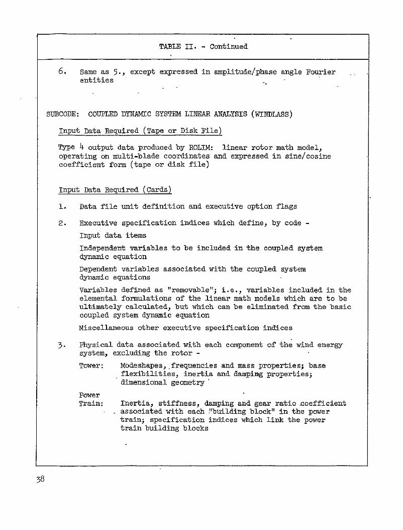
TABLE II - Continued
6 Same as 5 except expressed in amplitudephase angle Fourier entities
SUBCODE COUPLED DYNAMIC SYSTEM LINEAR ANALYSIS (WINDLASS)
Input Data Required (Tape or Disk File)
Type 4 output data produced by ROLIM linear rotor math model operating on multi-blade coordinates and expressed in sinecosine coefficient form (tape or disk file)
Input Data Required (Cards)
1 Data file unit definition and executive option flags
2 Executive specification indices which define by code -
Input data items
Independent variables to be included in the coupled system dynamic equation
Dependent variables associated with the coupled system dynamic equations
Variables defined as removable ie variables included in the elemental formulations of the linear math models which are to be ultimately calculated but which can be eliminated from the basic coupled system dynamic equation
Miscellaneous other executive specification indices
3 Physical data associated with each component of the wind energy system excluding the rotor -
Tower Modeshapes frequencies and mass properties base flexibilities inertia and damping properties dimensional geometry
Power Train Inertia stiffness damping and gear ratio coefficient
associated with each building block in the power train specification indices which link the power train building blocks
38
TABLE II - Concluded
Control System (Model includes dynamic characteristics of power
machinery power machinery controls power generating reflected torques and network elements) -Loop specifications transfer functions and gains
Pod (Nacelle) - Stiffness and inertia properties geometry at rotor tower and power train interface locations
4 Harmonic coefficients required to define dynamic shaft and blade loads produced by subcode PROCES
Output Data Produced (Line Printer)
1 Linear operators in ccupled system dynamic equation
2 Linear operators in removable variable equation (solvable from results of coupled system dynamic equation)
3 Eigenvalues and eigenvectors (reflecting coupled system stability) computed from the homogeneous portion of the dynamic equation
4 Time-history responses of selected system independent and removable variables representing the coupled system perturbation responses from the trim condition responses calculated by MOSTAB-HFW
5 Time-history responses periodic blade root loads superposition of trim loads computed by MOSTAB-HFW and perturbation coupled dynamic loads
39
TABLE III - METHODS OF DYNAMIC ANALYSIS-- ROTOR SYSTEMS
ADVANTAGES DISADVANTAGES
TIME-DOMAIN SIMULATION
s MANY DOF AND NONLINEARITIES EXCESSIVE COMPUTER COSTS
CONSTANT RE-SOLUTION FLEXIBLE PROGRAMMABILITY DIFFICULT STABILITY
EVALUATIONS NUMERICAL INSTABILITY
HAZARD
FREQUENCY-DOMAIN SOLUTION STANDARD PROCEDURES
CLEAR STABILITYEVALUATION CONSTANT COEFFICIENTS REQUIRED
-e-COMPONENT MODELS QUASI-STATIC ASSUMPTION
MOSTABROLIM SYSTEM
ALL ADVANTAGES OF REQUIRES FLOQUET OR FREQUENCY-DOMAIN ROOT-PERTURBATION
STABILITY ANALYSIS - METHOD ANALYSIS LINEAR ANALYSIS
PERIODIC MATH MODELS HNIGH FREQUENCY ROTOR
MODES
4o
TABLE IV - VECTORS FOR NIND TURBINE COUPLED SYSTEM
DescriptionaSymbol
c c c Control system inputs to rotor (NC)
f Perturbation load on rotor due to freeing fixed shaft (6)
fEP External load applied to pod (mP6)
fEPR Load at podrotor interface point applied topod (6)
fEPT Load at podtower interface point due to elasticdeformation of pod (6)
(NT6)fET External loads applied to tower
fH Total load on moving hub at rotorpod interfacepoint (6)
(6)fTP Load at podtower interface point applied to tower
fo Fixed shaft load applied to hub mass - from MOSTAB-HFW(6)
f Total moving shaft load applied to hub mass (6)0
h2 b External inputs to control system (iH)
x x x Rotor shaft perturbation motion (6)
X p Pod grid point displacements (NP6)
XT xT Displacement acceleration of tower grid points (NT6)
xTr7 p Displacement icceleration of towerpod interface point (6)
y Rotor degrees of freedom (NY)
a Control system degrees of freedom (NA)
YB Power train gear box reaction torque applied to pod (NBOX)
7C Control system torque applied to power train (1)
7cp Control system torque applied to pod (NGCP)
aItems in parentheses are vector length (see Table VI)
41
TABLE IV - Concluded
Symbol Description
rEP
7RPT
sect
(Power
CRPTV cPFT
External torque applied to power train (NPHI)
Power train torque applied to rotating hub mass
Tower base degrees of freedom (5 or 6)
Tower modal coordinates (NMv)
train independent degrees of freedom (NrnI)
Rotor rotation speed and acceleration perturbations (1)
()
4j
bull j
Rotor azimuth angle (1)
Rotor speed and acceleration perturbations (1)
42
TABLE V - OPERATORS FOR WIND TURBINE COUPLED SYSTEM
Symbol Description
AUo Control system operators
B3 BEQ BNj Damping operators for power train equations
BP BRW BC
B h) Control system operators for external input h
BI B B- Y Y y
Control system operators for rotor degrees of freedom y
B B Control system operators for rotor velocity and acceleration a
D D- Relate control system degrees of freedom to rotoraYcontrol variables
ECp Rotational transformation and partitioning operator for control system torques applied to pod
EEX Rotational transformation matrices for externally applied pod loads
Rotational transformation operator for pod loads at
EpR the rotorpod interface point
EppT Rotational transformation and partitioning operator for power train gear box torques applied to pod
ETp Rotational transformation matrix to express tower loads and deflections in the pod reference system
EXp Rotational transformation and partitioning operatorPR for pod deflections at the rotorpod interface point
E Relates control system degrees of freedom to generatora torque
FT Tower modal force participation factor for external tower loads
F Tower modal force participation factor and partitioning I operator for load at towerpod interface point
43
TABLE V - Continued
Symbol Description
G
GI
Tower grid point geometric operator for exterhal tower loads Tower grid point geometry and partitioning operator
for load at towerpod interface point -
GT Tower grid point geometric operator for external tower loads
IC Partitions generator torque 7yC reaction to appropriate gear box
IEP Partitions main gear torques to power train dofs
IEPT Applies the podtower interface load to the approprpod degrees of freedom
te
IPF
PT
Partitions reactions applied by the rotor to the pod
Partitions out those pod degrees of freedom at the podtower interface point
XO Partitions fixed shaft loads fo to rotorpod interface point
I
IXT
Partitions fixed shaft torque from f to power train
Partitioning operator for motion of towerpod interface point
Partitions out the five rotor shaft displacements that ate compatible with the pod
Y I Iy
Partitioning operators for moving shaft degrees of freedom
JB JP5
J
JEQ JN
JR JqP
Inertia operators for power train equations
Effective inertia of tower base including mass
by tower
loading
JH Rotor polar moment of inertia
44
TABLE V - Continued
Symbol
JX
K
B KEQ KN Kp) KR -K (
KpPPod
KO
M
MH
Ma
M
P
P
Q RcR R
Rf
Rj
U
UB
Description
Partitioned rotor polar moment of inertia
Power train shaft torsional stiffness operator or tower base stiffness operator
Stiffness operators for power train equations
stiffness operator or power train stiffness operator Differential stiffness operator for fixed shaft load in moving hub coordinate system
Rotor acceleration operator from ROLIM
Non-spinning rotor hub mass matrix
Pod mass matrix transferred to towerpod interfacepoint
Tower grid point mass loading on tower modes
Tower modal mass loading on tower base
Rotor velocity operator from ROLIM
Relates control system response to torques on the pod
Rotor displacement operator from ROLIM ROLIM operators for applying control inputs to rotor
ROLIM operator for applied rotor shaft load
ROLIM operators for changes in rotor speed andacceleration
Unity 6 x 6 operator
Unity operator for power train gear box torquereactions
45
TABLE V - Concluded
Symbol Description
U Unity-operator for rotor controls c c and -
UCp Unity operator for control system torque reaction to pod 7 Cp
UT Unity operator for tower degrees of freedom
U Unity operator for tower modal degrees of freedom
U1 Unity I x 1 operator
W Tower modal frequency operator
X Tower mode shapes fixed base
46
TABLE VI - VECTOR LENGTHS FOR WIND TURBINE COUPLED SYSTEM
Symbol Description
NA Control system degrees of freedom
NB Tower base degrees of freedom (5 or 6)
NBOX Power train gear boxes
NC Rotor control degrees of freedom
NEV Eigenvalues in tower modal model
NGCP Interface degrees of freedom between pod and control system
NH External inputs to control system
NPHI Power train gear block elements and independent degrees of freedom
NP6 Pod degrees of freedom (6 times the number of grids)
NT6 Tower degrees of freedom (6 times the number of grids)
NY ROLIM rotor model degrees of freedom
47
TABLE VII - TEETERING HUB DESIGN CONCEPTS - WEIGHTS AND OTHER DESIGN DATA
Teetering concept
Weight a outboardShifto Hub (M
Undersling )
Stop Mechanism
Description Comments
Long Yoke 15100 -0178 0478 Hydraulic Cylinders
Long yoke places teetering axis near overall cg
Requires modified outboard hub plateheaviest concept
Short Yoke 9800 0178 -o386
Hydraulic Cylinders
Short yoke places teetering axis near shaft face for minimum weight
Negative undershysling is unconventi6nal
Linkage 10200 0381 O914 HyIdraulic Cylinders
Basic four-bar linkage places teetering axis at classical under-slung location
Least conventional teetering aais translates slightly as linkage moves
a Stop mechanism not included
TABLE VIII - BLADE ROOT FLEXURES - SUMMARY
DESIGN
Material Modulus of Elasticity (1010 Nm2 ) Dimensions (m) Flexure Weight (N blade) Total Assembly Weight (N blade) Divergence Speed msec from TE 45 degrees
Inplane Natural Frequency (per-rev at n = 4aradsec) Inplane Bending Moment Range (N - m x iO3)
2 -8 ) Maximum Flexure Inplane Stress (N x
Flapwise Natural Frequency (per-rev at a= 4aradsec) Maximum Flapwise Bending Moment (N-m x 103) Flapwise Bending Moment Reduction Maximum Flexure Flapwise Stress (Nm2 xlol
Maximum Deflection When Passing Tower (i) Deflection Increase
Zero Load Steady Conet (angle from vertical)
A B Steel Steel
Unsymmetric Symmetric
4340 Steel HT to 1lxlO9Nm2 shy21 21
074x147xl46 12 dia x 152 1748 1792 6227 6227 474 6o8
191P 1-50P +77 to -85 +81 to -119 324 69
150P 191P 515 895
67 43393 531
0 67 39 -43
4 degrees 5 degrees
C D Fiberglass Fiberglass
Unsynmetric Symmetric
Unidirectional Fiberglass 3-9 39
IOx198x91 16 dia x 91 578 578
4581 4581 456 581
191P 150P +34 to -85 +81 to -119
131 296
150P 191P 515 85
67159 221
0 o6 -4
4 degrees 5 degrees
Preliminary - Dimensional revisions (to stiffen) are required to achieve 15P lowest frequency Over IAOSTAB prediction for current Mod-O rigid shaft (Figure 4 Reference 8) Rigid Shaft Mod-O prediction is +34 to -85 N - m x 10-3 (Figure 44 Reference 8) Rigid Shaft Mod-O prediction is 07 m at = 10 degrees (Figure 45 Reference 8) t Assumes 7 degrees precone zero load steady cone for current Mod-O = 6 degrees from vertical
FIGURE 1- COUPLED DYNAMICS ANALYSIS (MOSTAS) - GLOBAL ARRANGEMENT
I DATA FILE INDICES
TRIM RESULTS S OPTION INCLUDING POWER FLAGS EXTRACTED GRADIENT ARRAYS PROCES
DATA S READ AND PRINT FILE LOADS amp MOTION
DATA FOR TRIM LOADS AND DATAIN MOSTAB-HFW 0 PERFORM HAR- MOTION DATA
READ BASIC DATA S COMPUTE CONSTANTS MONIC ANALYSIS TIME AND INPUT DATA FILE S FIND TRIM OF BLADE AND REQUENCY
VERIFYGENERATE PROCES SHAFT LOADS DOMAIN PRINT DATA DATAD DATA
OUTPUT GRADIENT P MISC DATA-ARRAYS IICONDITIONING
ROLIMX PROCEDURES
GENERATE BASIC DATA OTN REQUIRED BY ROLIMDATAROLIM A
READ HARMONIC LOAD ATAFROM PROCES PHYSICAL DATA ANALYSIS
FOR WIND TUR- U A NORMALIZE DATA LINEAR ROTORFINE CQMPO- WINDI AqqNENTS~tEXCEP1 DATAFILE FOR SOUGHT MODEL ~RO NENTS tEXCEPT ASS
COUPLED DYNAMIC SYSTEM LINEAR ANALYSIS FREQUENCYTAIGOE N RO-CONTENT GOROTOR) COMPUTE MULTIBLADES BASIC LINEAR S WIND TURBINE SYSTEM COMPONENT MATH 5 EXPAND SINGLE- COORDINATES
MODEL SPECI- MODEL BLADE DATA TOFICATION 0 LINEAR SYSTEM COUPLED DYNAMICS SFULL ROTOR INDICES EQUATION 0 COORDINATE
I EXECUTIVE S STABILITY (EIGENVALUES AND OPTION FLAGS EIGENVECTORS) RL E PRINT
COUPLED LOADS AND MOTION RESPONSE STABILITY ANALYSIS RESULTS
-ISYSTEM COMPONENT TIME-HISTORY RESP0NSES
IBLADE ROOT LOADS- TIME HISTORY RESPONSE( WITH MOVING SHAFT AND CONTROL
FIGURE 2- TIME AND FREQUENCY DOMAIN ANALYSIS METHODS
STABILITY ANALYSIS METHODS
i [ poundIL 10 -- _ 4 - - J
_ _
1 -07 --- ----shyvpi-i z v i I 10 I
TIME DOMAIN
IM
20 _I C 100 10 I I
COMPLEX AMPLITUDE PLANE 0 iA I
-10 -130RE - aft -200 -100 I -20 sect X-- - -170-0 shy
-30 - HS-21
t-lo -40 -
01 05 1 5 10 290 FREQUENCY
ROOT LOCUS PLOT BODE PLOT
FREQUENCY MIN
51
FIGURE 3- BASIC MOSTABIROLIM ANALYSIS PROCEDURES
PRINT STABILITY DERIVATIVES
PERFORMANCE ETC
OTABEECUiIE_SYSTEMF_ INPUT TRIM-SEARCH LINEAR R0 DATA __LOGIC MODELLING LI LINEAR CARDS GLOGIC - MATH
BLADE PROGRAM PROCESS SYSTEM MOTIONS AND PRINT amp ANALYZE COMPONENT LOADS BLADE LOADS amp
MATH MODELS MOTIONS
ROLIMMODELSRVS]) ROLIMPROCESSOR-MODELS V EXPAND TO MULTI-BLADE ROTOR TMIE OR FREQUENCY s INTERFERENCE COUPLINGF MULTI-BLADE COORD XFORM
FIGURE 4 - ESSENTIAL ELEMENTS OF MOSTAB MATH MODELS
EXECUTIVE SYSTEM i
offEA VELOCITIES
REQUESI FORCES AND VELOCITIES
BEaiE INTERFERENCE
ACCELERATIONS MOMENTS ACCELERATIONS VELOCITY
CONTROLS CONTROLS amp LOADS FIELD
------------------ ------- ----------shy j-
IYNMOD ( ^WASH
EXECUTIVE CODE FORCE
TYPE OF ERO ARE TIR EN AEROELASTIC I ITREECANALYSIINERERNC
7P Al~q~I VELOCITY MODELS 6 DOF WAKE
BODY LIFT WEPIMO E
AERODYNAMIC LIFTING I SI INTEGRATION I MODEL
MULTI-DOF
BODIES SURFACES WAKEMODELSWEP AEMDE
RADIAL AND BLADE
AZIMUTHAL - AEAERO INTEGRATION
-------------------- 4------ --shy MOSTAB-C I MOSTAB-HNE I---------------------4-----------------------shy
FIGURE 5- MOSTAB EXECUTIVE LOGICAL PROCEDURE
COMP E FORCES MODamp INTERFERENCEASSEMBLEREALIEA IWTR TE
VELOCITIES -
USE ESTIMATES
ASSEMBE LINEAR MODEL OF FORCE ampINTERFERENCE
SOLVE LINEAR MODEL FOR NEW-
ESTIMATES
MT MODELS
INTERFERENCE MATH
MODELS
LOAS AND E___ MOTIONS -
FINAL CALLS
NO TIMDLINEAR MATH MODELS-LOADS
MOTIONS
ROLIMX I NEAR MODEL
54
- FIGURE 6- FUNDAMENTALS OF ROTOR ANALYSIS
~BLADE
COORDINATES SHAFT REFERENCE LINE
~~ BLADEgt ilts AXES
ROTOR AXES
ATTRIBUTES
SIMPLE ROTOR ANALYSIS AEROELASTIC ANALYSIS
ONE DOF CONSTRAINED TO A USER-SPECIFIED NUMBER
MOTION PARALLEL TO SHAFT OF DOF BLADE ELEMENT MASS AND
s BLADE ELEMENT A POINT INERTIA TENSOR
MASS SIX-DOF ELEMENTAL MODEL
BOTH
STATIC AERO-STALL AND COMPRESSIBILITY
FUNCTION OR TABLE-LOOK UP
55
FIGURE 7- AEROELASTIC BLADE ANALYSIS
SINGLE BLADE MODEL ISOLATED BY SHAFT WITH PRESCRIBED MOTION
BLADE ELEMENTS MOVE INSIX DOF
MODAL MODEL TRANSFORMS BLADE MOTION TO NORMAL COORDINATES
MODEL REQUIRES INPUT
-- MODESHAPES (6DOF) -- FREQUENCIES
-- INERTIAL PROPERTIES -- NUMBER OF DOF -- INITIAL SHAPE
BLADE-MODE INITIAL CONDITIONS DETERMINED
BY ITERATIVE PROCEDURE
GIMBAL ANALYSIS USES ITERATIVE PROCEDURE
AND SINGLE-BLADE MATH MODEL
56
FIGURE 8 - GIMBAL ANALYSIS
GIVEN SHAFT AND AIR
MOTIONSCONTROL
TRANSFORMATION
SPRESCRIBED GIMBAL MOTION Ji I SPECIFIED - -
SINGLE-BLADE MODJELshy
a BLADE MOTION
GIMBAL ERROR VS AZIMUTH
ALE YSNEAR MODEL VALID AROUND SOLUTIONESA p_
gtCONDITION NO CALCULATE SHAE LOADS
LINEAR MATH MODEL GIMBAL ERRORVS GIMBAL T
AND MODAL fOFI LOADS TO REFERENCE AXESI
SOLUTION OF LINEAR MODEL REUR I FINAL BLADE MOTION F RETURN
o ZERO GIMBAL ERRORJ
s NEW PRESCRIBED GIMBAL
MOTION
57
FIGURE 9 - ADVANCED SHADOW MODEL
RADIAL
NOMINAL INTEGRATION
SEGENSIZSETO
I NAS
REDUCED
SHADOW VELOCITY SECTOR SIZE
SPECIFIED FOR EACH
REGION
i11IfIIIfIf111IIIIIi I
rp
SHADOW PROFILE SPECIFIED AS FUNCTION
OF AZIMUTH AND RADIUS - KEYED TO
TOWER DRAG-ARBITRARY PROFILE
58
FIGURE 10- MOSTAB OUTPUTS
TRIM CONDITIONS
CONTROLS
LOADS MOTIONS
WAKE
COMPREHENSIVE LOADS AND MOTIONS
0 TIME AND FREQUENCY DOMAINS
SIX DIRECTIONS AT ALL RADII
LINEAR MATH MODELS
o STABILITY AND CONTROL DERIVATIVES
-- OVERALL
-- INDIVIDUAL COMPONENTS
0 ROLIMX DATA
59
FIGURE 11 - STEPS INROLIM PROCESS
A ROLIMX PROCEDURES USE MOSTAB MODELS TO SYNTHESIZE
LINEAR OPERATIONS FOR
o BLADE GENERALIZED FORCING FUNCTIONS
o SHAFT LOADS
s WAKE VELOCITIES
AS FUNCTIONS OF
BLADE MODAL COORDINATES (SINGLE BLADE)
s SHAFT MOTIONS
CONTROLS
o AIR VELOCITIES
B SINGLE-BLADE LINEAR MODEL EXPANDED TO FULL ROTOR -
PHASE SHIFTING PROCEDURE
C ROTOR AND WAKE MODELS COMBINED WITH RIGID-BODY SHAFT EQUATIONS TO FORM ROLIM EQUATIONS
D ROLIM EQUATIONS TRANSFORMED TO MULTI-BLADE COORDINATES
E PERIODIC OPERATORS-CONVERTED TO FREQUENCY DOMAIN
6o
FIGURE 12 - THE ROTOR LINEAR MODELLING PROGRAM
ROLIM
FINAL MODEL
My+By+ KY= YC+YC+YC+YS+Y c c c 2 S2
SHAFT DOF
BLADE MODAL
DOF ALL
y = MODES INALL CONTROLSc = BLADES
OTHER AERO-
ELASTIC DOF
Qs2 ROTOR SPEED AND ACCELERATION
PERIODIC OPERATORS PRESENTED AS TIME FUNCTIONS OR
SPECTRA - MODEL GENERATED INSIX OPTIONAL CONFIG-
URATIONS INCLUDING MULTI-BLADE COORDINATES
61
FIGURE 13 - EXAMPLE ROLIM PRINTOUTS
0
s X-WING AIRCRAFT HELO MODE ROTATING COORDINATE SYSIM
SIMPLE ALRO TEST CASE JULY 196
PSI 00
300 600 900 1200 1500 1800 2100 2400 2700 3000 3300
nC( 1 1) -704s3E-01 -33000E-01 l5152E-02
-70433E-01 -33000-01 15152E-01
-704-23E-01 -33000E-01 1515E-01
-104336-01 -33000E-01 151plusmn2L-01
nt 2 1) OD( 3 1) 54183E-01 11603E-02 8t40E-01 -18242E-02 9 3 080t-01 -140704-02 59183E-01 11603L-02 8b540t-01 -1hL42b-02 93010E-0I -14070E-02 b910bL-01 11o03E-02 0tgt40E-O1 -IL32n2E-02 3(YiE-U1 -14070E-02 59183E-0 11o03E-02 8Lf40L-01 -11242E-02 93(fi06-o1 -14070E-02
ODI 4 1) OD( 59 1) 791k6E-01 1606E+00 23717E+00 71785E-01 22993E+00 -13305E+00 9126E-01 b656E+G0 23717E+O0 7178LbE-01 2i993E+00 -13305t+00 7912oE-01 1ou5bL+UO 2371h+GO 717bbb-01 229931+0 -133051+00 7Qlli-01 lbubb+00 23717E+00 717bbL-01 22993E+00 -133G5h00
ON 6i 1) 30459E02 30437t+02 30457E+02 30459E 02 30437E+U2 30457E+02 30459E+02 304371+02 30457L+02 3045YE+02 30437E+02 30457E+u2
DD( 7T 1) 15851 -02 973OOE-03 24499E-02 23245E-02 12222E-02 12635E-02 1blOE-O2 21440E-02 23375E-02 25U44E-u2 39t5E-02 39354E-02
ODI 8t 1) 21147E-O1 24bbbE-01 2b701-d 2Y9t5E-OI 2754L-01 Z673UE-01 25bb7E-01 23b52E--61 25744 E-01 29bUCjt-1 235bb-O1 1939-0I
PSI 00
300 600 900 1200 1500 1800 2100 2400 2700 3000 3300
001 9 1) 22245E-02 12 2E-02 12t3bE-02 16150E-02 21440 -02 23375E-02 25244E-02 39655E-02 39354E-02 1SR5E-02 i7300E-03 2449k-02
U)(10 1) 00(11 1) Z7ibh-01 1blhOE-02 27546-01 Z140E-02 26730E-61 23375E-U2 25bbE-ul 25844E-02 23b52L-01 39t55E-O 2574-L-01 3935E-02 29CUOE-01 158516-02 25356E-01 97fOE-03 193136L-01 24499E-C2 21147b-01 23245E-02 24656E-02 1122E-Oz 2h470F-01 126356-02
D1(12t 1) 25bblE- 23t5gE-01 25144L-01 24boOE-01 k5356E-01 1939hE-01 21147E-01 24t5LL-01 2b3702-01 27955E-01 27554E-01 26730E-01
OD(13p 1) 2Sbrth-02 39655E-02 39354E-02 15bbE-02 97300E-03 2444E-02 23245E-02 12222E-02 12635E-02 1615O-02 i440L-o
23375E-02
OPtle 11 29bbOL-01 25356-l01 19396E-01 21147L-01 24656h-01 263706-01 27955E-01 27554k-01 2673UE-O1 258t7E-01 23652E-01 25744E-01
FIGURE 14 - TOWER MATH MODEL
Yi
FLEXIBLE STRUCTURE (FIXED BASE)
z
MOVABLE BASE MODEL BAS
-7777770
z 0
LINEAR TOWER MODEL SUPERPOSITION OF
9 -MODAL MODEL OF TOWER MASS -ELASTIC
STRUCTURE WITH FIXED BASE
o RIGID BODY MODEL ON ROTARY BASE
63
FIGURE 15 -SAMPLE CONTROL SYSTEM MODEL
COLLECTIVE
PITCH CONTROL
WIND] WIND
TURBINE ROTOR MODEL
u v
V
q r--
ROTOR
DOF
----------------WINCON yi
-------------------- r
+ s + 2 ~
I
ALOITM
ALOITM
----- --
IPT - -- -
INUT
IROTOR
SSPEED a IP
Ie
64a
GiENERAL monll INERTIA
I Ii s STIFFNESS s DAMPING
s GEAR RATIO
I I
I
I I [] I
-------------------------
dega I
m-ROTOR TORQUE -- -shy-
INCREASOR r I Ij
E 3VBELTS
GEARING
FIGURE 16 - POWER TRAIN DYNAMIC MATH MODEL
FIGURE 17 WIND TURBINlE SYSTEM BLOCK DIAGRAM
-PITC CONROLMAflOELSTIC ROTOR
Aaamp E]y+BBBf11fln+Eif (C-1) State Space Model I
UccDc(C-) P-Qy- IY+Re++R+RA~+n (R-12)
1Pa (C-1) Qadnatlc Space ModelshyyW+Py44v = Eff+Ra ctc+Pfllf (R-12)
=~7C
1ka ) CR-8)
TE 9 (R-9)
lx Ix t
PNE TRAIN__ I f H tJTC=E(+ C Eifurplcc PP PPPP Mj=K0 ) XIf 0 -GTf6 1X0 f0 CR-i)
VPP C-vrfrvp ThPR - RX(R-2)D-i)
U1RTrR+R-E ip+p~~lpPp (D-2) S J+I4toUijo (R-3)
lpM=U1_ (R-4)URB~1 XT uyp ( (-) U1___________ PT_____________ Uj Rpu3i (n-5) UffI-U31 (a-10)
u RPt (n-6) UA-uii CR-fl)
KI n+mt+wX+E9 = Er~xP (Pp2)
70CP UXPR - LEXR (P-3)
TOM POD MASS
UJrIW44N = FTfET-FIfTn (Tn-1)
GjtrTG t T P I um + E TpT (P-5)
U = Xj + G5 (T-3) T J 4KS- 1 f
2 UTxT= X 9+ G9 (T-4)
uT mInxTr (T-5) = (r-6)U I~X
Q 4 4 66
FIGURE 18 - LONG YOKE TEETERING DESIGN
10 a (39 12 in)
1 8 1 2-7nL-n)
- elI
Kf- ___-
0I
i bull8 LuIj
CTCO
FIGURE 19 - SHORT YOKE TEETERING CONCEP tTBD-
V 686 m _ 051 m- (27 in) (2in)
-(19 Od Co495 n in)
1109 in (43 in)
~-(7in+ 7c 40z1 178 m
FIGURE 20 - LINKAGE TEETERING CONCEPT
_--_ r
(36-rinw
o 81 m (1 in)
FIGURE 21 - ROOT OUT-OF-PLANE MOMENT
Conditions V = 12msec 9 = -80 n= 42 radsee = 7750
150 Legend (MOSTAB-HFW)
00 Rigid Shaft No Teeter
125- -Teeter Zero Undersling
I0000-
75 -Teeter
Teeter 046m Undersling
092m Undersling
Io Test Data Reference II Figure lIla
H0 0 3
o O 360 20 I 30 33 360 -5
-25- Position Deg
-2t -2s-Azimuthal
FIGURE 22 - ROOT IN-PLANE MOMENT
40
20 20 -
0t 60 90 120 80 210 240 270 330 J0 o A
1-401
- Legend (MSTAB-mW)
-60- Rigid Shaft No T
-60-Teeter Teeter
Zero tlndereling o46m Unersling
Teeter 092m Underling
00 Test Data Reference 11 Pigure ii
-80-
Azimuthal Position Deg
FIGURE 23 - BLADE TIP DEFLECTION
125 40
075
0s
05-N
30
20
I-
Nshy
00 o n V 4 a
4 0
p
-0-25-
F
E
44
S-0-
Agimuthal oston
30 60 9020 50 802 240 Conditions V= l2nsec A = -8deg0= 42 radfsec = t750
s ________ igid Shaft No Teeter
Teeter Blade Bending Only
270 300 I
33
bull
360
Teeter Blade Bending + Hub Rotation
-20 - -shy
-075
-301
FIGURE 24 - BLADE MOMElT REDUCTION EXPECTED FROM TEETERING AS A FUNCTION OF PRESEkT HUB SUPPORT STIFFNESS
50 - shy
4o
318
30
24
S 20 i0 - - _i___e_
20 -
Range tox
Present Mod-C
0 001 005 01 02 08 10 10T t t T
Rigid twsort (120) (15) (1125)
Presnt bktio of Blad6 Sfts to popor tUffmmu 1It$ W)6
FIGURE 25 -ELASTIC INTERFACE
FLEXURE A
-SEC-T 8-LI_
0074m x 0J-47m x 14 6m long
4340 srre liT MOOO-To 5
74YCA YSZLO
7h
~FIGURE 26 -
ELASTIC INTERFACE
FLEXURE B ---SACT2CA C-Cshy
c C
COLLE-- PLIo 01m da x l52m long
73 D A I M -L
- FIGURE 27 -
ELASTIC INTERFACE
FLEXURE C - SC7YON 4- shy
ill
SPLIT CZLtET
FIBERLASS
S 39 Y 7r
BEAIMCStlppCns76
REVERSE CONING
STRAP-FOR ST ELECRIC GROUND
1O1m x 0198m x 091m long
J i
3WIECVONA9tB ISLt
FIGU= 28 -ELASTIC INTERFACE FLEXURE D
17~
O16m dia x 091m long
Ly
UNpPrOflf pr ASS
FIGURE 29 - ROOT OUT-OF-PLA14E BEDING MOMENT
175 25 Conditions V= 12msec ep -8S= 42 radsec Vs9 plusmnT Legend (MOSTAB-HFW)
50 Root Flexure Unmatched Stiffness
00- - Root Flexure Matched Stiffness
125 Mod-n Baseline Rigid Shaft
7S- Teetered Hub Zero Undersling
00 T
90 75- II
50-H75 if0251
2-I
o 00 0 A I
306 S 20 150 06- -210 240 -gt7 3M0 360
-25 -25- Azimuthal Position Deg
-50
FIGURE 30 - ROOT IN-PLANE BENDING MOMENT
00- 75 ConditionsV=12msee j = -80 9= 42 radsec$ s plusmn750
-- I ( MOSTAPHFW Results)-gend
Hoot Flexure Unmatched Stiffness75 - 50Leed--oot Flexure Matched Stiffnes
50 Mod-O Baseline Rigid Shaft
Teetered25 Hub Zero Underalinj
25 -_ - - -
IiI1 I
300~ 60 TO 720 180 20240 270 30033fl
-25 ~ 2Azimuthal Position Deg
~-s0
-00 -5shy
-12- -00
0 o
FIGURE 31 - BLADE TIP DEFLECTIO11
25
0-
0
30 -
Conditions V= 12msee a==480= 12 radsec p
Legend (I4OSTAB-HF4)
Root Flexure Urmatched Stiffness
Root Flexure Matched Stiffness
Mod-O Baseline Rigid Shaft
Teetered Hub Zero Undersling
= 750
S075-
~20
0 00
0 I 4
~0 -
H S30 90
H0 120 150 80 20 240 270 300 A0 36
- 0AzimuthalPoion g
-05 -2o
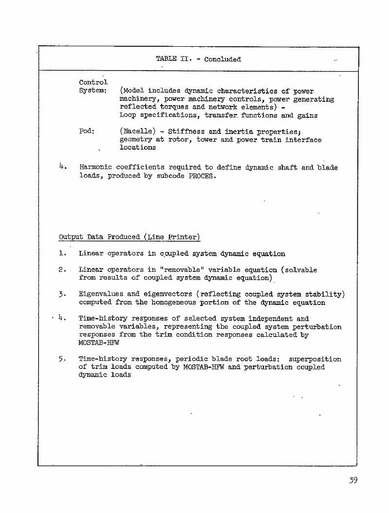
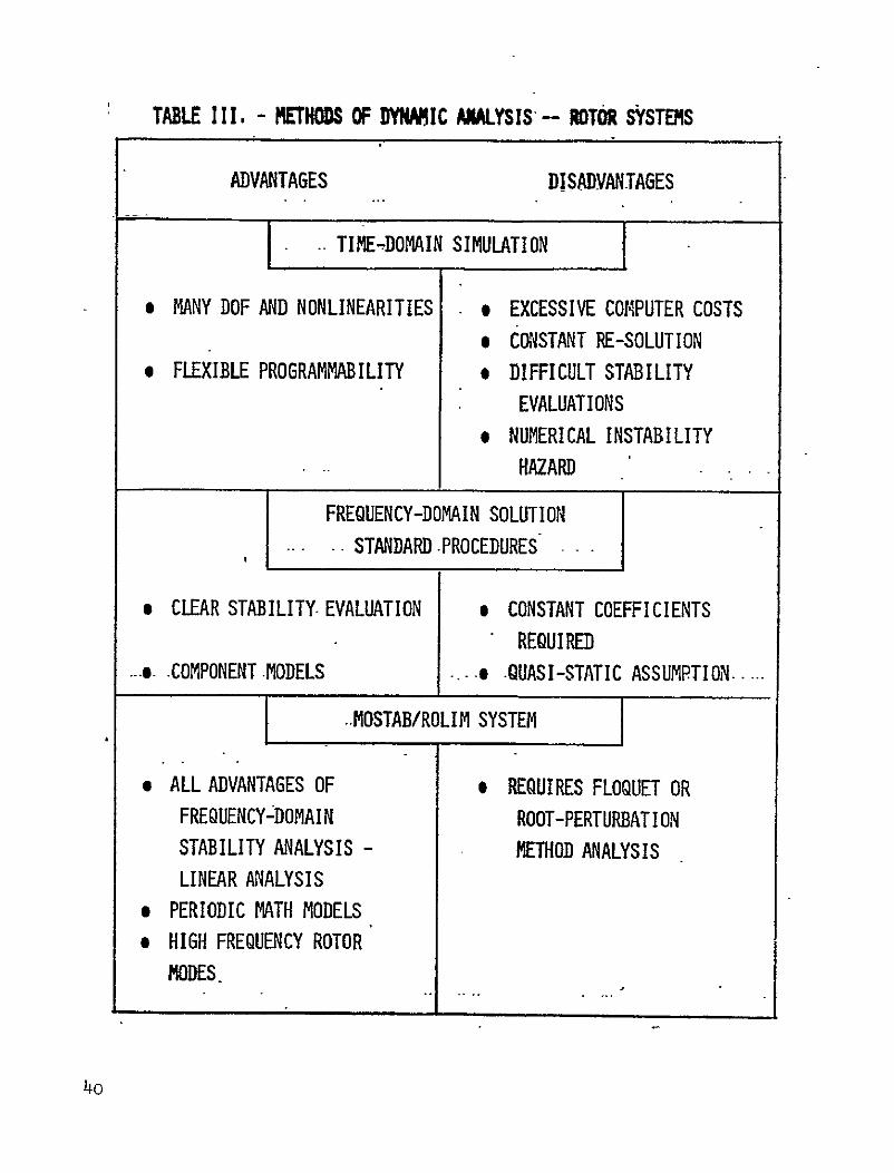
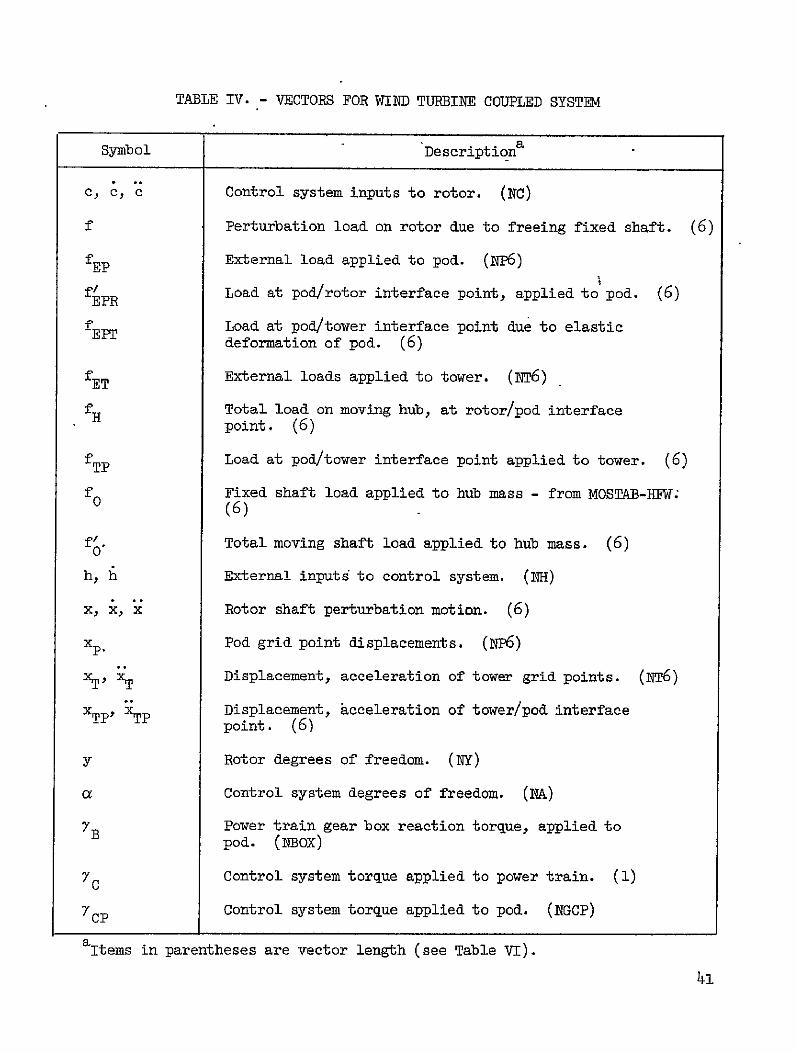
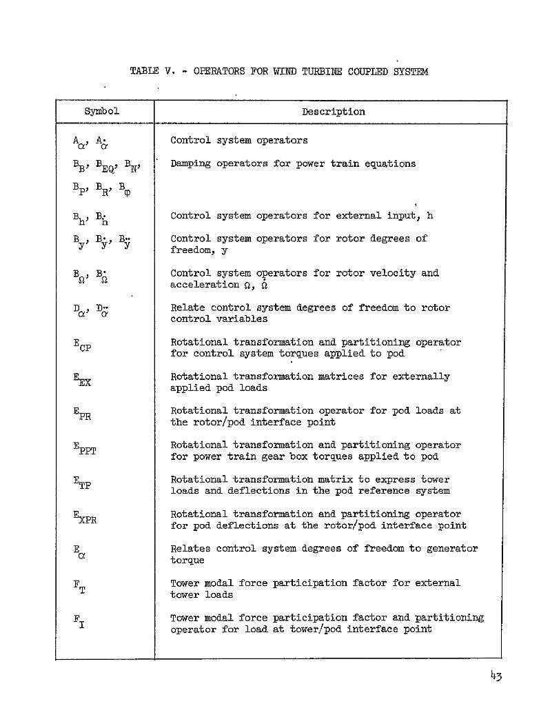

TABLE V - Continued
Symbol Description
G
GI
Tower grid point geometric operator for exterhal tower loads Tower grid point geometry and partitioning operator
for load at towerpod interface point -
GT Tower grid point geometric operator for external tower loads
IC Partitions generator torque 7yC reaction to appropriate gear box
IEP Partitions main gear torques to power train dofs
IEPT Applies the podtower interface load to the approprpod degrees of freedom
te
IPF
PT
Partitions reactions applied by the rotor to the pod
Partitions out those pod degrees of freedom at the podtower interface point
XO Partitions fixed shaft loads fo to rotorpod interface point
I
IXT
Partitions fixed shaft torque from f to power train
Partitioning operator for motion of towerpod interface point
Partitions out the five rotor shaft displacements that ate compatible with the pod
Y I Iy
Partitioning operators for moving shaft degrees of freedom
JB JP5
J
JEQ JN
JR JqP
Inertia operators for power train equations
Effective inertia of tower base including mass
by tower
loading
JH Rotor polar moment of inertia
44
TABLE V - Continued
Symbol
JX
K
B KEQ KN Kp) KR -K (
KpPPod
KO
M
MH
Ma
M
P
P
Q RcR R
Rf
Rj
U
UB
Description
Partitioned rotor polar moment of inertia
Power train shaft torsional stiffness operator or tower base stiffness operator
Stiffness operators for power train equations
stiffness operator or power train stiffness operator Differential stiffness operator for fixed shaft load in moving hub coordinate system
Rotor acceleration operator from ROLIM
Non-spinning rotor hub mass matrix
Pod mass matrix transferred to towerpod interfacepoint
Tower grid point mass loading on tower modes
Tower modal mass loading on tower base
Rotor velocity operator from ROLIM
Relates control system response to torques on the pod
Rotor displacement operator from ROLIM ROLIM operators for applying control inputs to rotor
ROLIM operator for applied rotor shaft load
ROLIM operators for changes in rotor speed andacceleration
Unity 6 x 6 operator
Unity operator for power train gear box torquereactions
45
TABLE V - Concluded
Symbol Description
U Unity-operator for rotor controls c c and -
UCp Unity operator for control system torque reaction to pod 7 Cp
UT Unity operator for tower degrees of freedom
U Unity operator for tower modal degrees of freedom
U1 Unity I x 1 operator
W Tower modal frequency operator
X Tower mode shapes fixed base
46
TABLE VI - VECTOR LENGTHS FOR WIND TURBINE COUPLED SYSTEM
Symbol Description
NA Control system degrees of freedom
NB Tower base degrees of freedom (5 or 6)
NBOX Power train gear boxes
NC Rotor control degrees of freedom
NEV Eigenvalues in tower modal model
NGCP Interface degrees of freedom between pod and control system
NH External inputs to control system
NPHI Power train gear block elements and independent degrees of freedom
NP6 Pod degrees of freedom (6 times the number of grids)
NT6 Tower degrees of freedom (6 times the number of grids)
NY ROLIM rotor model degrees of freedom
47
TABLE VII - TEETERING HUB DESIGN CONCEPTS - WEIGHTS AND OTHER DESIGN DATA
Teetering concept
Weight a outboardShifto Hub (M
Undersling )
Stop Mechanism
Description Comments
Long Yoke 15100 -0178 0478 Hydraulic Cylinders
Long yoke places teetering axis near overall cg
Requires modified outboard hub plateheaviest concept
Short Yoke 9800 0178 -o386
Hydraulic Cylinders
Short yoke places teetering axis near shaft face for minimum weight
Negative undershysling is unconventi6nal
Linkage 10200 0381 O914 HyIdraulic Cylinders
Basic four-bar linkage places teetering axis at classical under-slung location
Least conventional teetering aais translates slightly as linkage moves
a Stop mechanism not included
TABLE VIII - BLADE ROOT FLEXURES - SUMMARY
DESIGN
Material Modulus of Elasticity (1010 Nm2 ) Dimensions (m) Flexure Weight (N blade) Total Assembly Weight (N blade) Divergence Speed msec from TE 45 degrees
Inplane Natural Frequency (per-rev at n = 4aradsec) Inplane Bending Moment Range (N - m x iO3)
2 -8 ) Maximum Flexure Inplane Stress (N x
Flapwise Natural Frequency (per-rev at a= 4aradsec) Maximum Flapwise Bending Moment (N-m x 103) Flapwise Bending Moment Reduction Maximum Flexure Flapwise Stress (Nm2 xlol
Maximum Deflection When Passing Tower (i) Deflection Increase
Zero Load Steady Conet (angle from vertical)
A B Steel Steel
Unsymmetric Symmetric
4340 Steel HT to 1lxlO9Nm2 shy21 21
074x147xl46 12 dia x 152 1748 1792 6227 6227 474 6o8
191P 1-50P +77 to -85 +81 to -119 324 69
150P 191P 515 895
67 43393 531
0 67 39 -43
4 degrees 5 degrees
C D Fiberglass Fiberglass
Unsynmetric Symmetric
Unidirectional Fiberglass 3-9 39
IOx198x91 16 dia x 91 578 578
4581 4581 456 581
191P 150P +34 to -85 +81 to -119
131 296
150P 191P 515 85
67159 221
0 o6 -4
4 degrees 5 degrees
Preliminary - Dimensional revisions (to stiffen) are required to achieve 15P lowest frequency Over IAOSTAB prediction for current Mod-O rigid shaft (Figure 4 Reference 8) Rigid Shaft Mod-O prediction is +34 to -85 N - m x 10-3 (Figure 44 Reference 8) Rigid Shaft Mod-O prediction is 07 m at = 10 degrees (Figure 45 Reference 8) t Assumes 7 degrees precone zero load steady cone for current Mod-O = 6 degrees from vertical
FIGURE 1- COUPLED DYNAMICS ANALYSIS (MOSTAS) - GLOBAL ARRANGEMENT
I DATA FILE INDICES
TRIM RESULTS S OPTION INCLUDING POWER FLAGS EXTRACTED GRADIENT ARRAYS PROCES
DATA S READ AND PRINT FILE LOADS amp MOTION
DATA FOR TRIM LOADS AND DATAIN MOSTAB-HFW 0 PERFORM HAR- MOTION DATA
READ BASIC DATA S COMPUTE CONSTANTS MONIC ANALYSIS TIME AND INPUT DATA FILE S FIND TRIM OF BLADE AND REQUENCY
VERIFYGENERATE PROCES SHAFT LOADS DOMAIN PRINT DATA DATAD DATA
OUTPUT GRADIENT P MISC DATA-ARRAYS IICONDITIONING
ROLIMX PROCEDURES
GENERATE BASIC DATA OTN REQUIRED BY ROLIMDATAROLIM A
READ HARMONIC LOAD ATAFROM PROCES PHYSICAL DATA ANALYSIS
FOR WIND TUR- U A NORMALIZE DATA LINEAR ROTORFINE CQMPO- WINDI AqqNENTS~tEXCEP1 DATAFILE FOR SOUGHT MODEL ~RO NENTS tEXCEPT ASS
COUPLED DYNAMIC SYSTEM LINEAR ANALYSIS FREQUENCYTAIGOE N RO-CONTENT GOROTOR) COMPUTE MULTIBLADES BASIC LINEAR S WIND TURBINE SYSTEM COMPONENT MATH 5 EXPAND SINGLE- COORDINATES
MODEL SPECI- MODEL BLADE DATA TOFICATION 0 LINEAR SYSTEM COUPLED DYNAMICS SFULL ROTOR INDICES EQUATION 0 COORDINATE
I EXECUTIVE S STABILITY (EIGENVALUES AND OPTION FLAGS EIGENVECTORS) RL E PRINT
COUPLED LOADS AND MOTION RESPONSE STABILITY ANALYSIS RESULTS
-ISYSTEM COMPONENT TIME-HISTORY RESP0NSES
IBLADE ROOT LOADS- TIME HISTORY RESPONSE( WITH MOVING SHAFT AND CONTROL
FIGURE 2- TIME AND FREQUENCY DOMAIN ANALYSIS METHODS
STABILITY ANALYSIS METHODS
i [ poundIL 10 -- _ 4 - - J
_ _
1 -07 --- ----shyvpi-i z v i I 10 I
TIME DOMAIN
IM
20 _I C 100 10 I I
COMPLEX AMPLITUDE PLANE 0 iA I
-10 -130RE - aft -200 -100 I -20 sect X-- - -170-0 shy
-30 - HS-21
t-lo -40 -
01 05 1 5 10 290 FREQUENCY
ROOT LOCUS PLOT BODE PLOT
FREQUENCY MIN
51
FIGURE 3- BASIC MOSTABIROLIM ANALYSIS PROCEDURES
PRINT STABILITY DERIVATIVES
PERFORMANCE ETC
OTABEECUiIE_SYSTEMF_ INPUT TRIM-SEARCH LINEAR R0 DATA __LOGIC MODELLING LI LINEAR CARDS GLOGIC - MATH
BLADE PROGRAM PROCESS SYSTEM MOTIONS AND PRINT amp ANALYZE COMPONENT LOADS BLADE LOADS amp
MATH MODELS MOTIONS
ROLIMMODELSRVS]) ROLIMPROCESSOR-MODELS V EXPAND TO MULTI-BLADE ROTOR TMIE OR FREQUENCY s INTERFERENCE COUPLINGF MULTI-BLADE COORD XFORM
FIGURE 4 - ESSENTIAL ELEMENTS OF MOSTAB MATH MODELS
EXECUTIVE SYSTEM i
offEA VELOCITIES
REQUESI FORCES AND VELOCITIES
BEaiE INTERFERENCE
ACCELERATIONS MOMENTS ACCELERATIONS VELOCITY
CONTROLS CONTROLS amp LOADS FIELD
------------------ ------- ----------shy j-
IYNMOD ( ^WASH
EXECUTIVE CODE FORCE
TYPE OF ERO ARE TIR EN AEROELASTIC I ITREECANALYSIINERERNC
7P Al~q~I VELOCITY MODELS 6 DOF WAKE
BODY LIFT WEPIMO E
AERODYNAMIC LIFTING I SI INTEGRATION I MODEL
MULTI-DOF
BODIES SURFACES WAKEMODELSWEP AEMDE
RADIAL AND BLADE
AZIMUTHAL - AEAERO INTEGRATION
-------------------- 4------ --shy MOSTAB-C I MOSTAB-HNE I---------------------4-----------------------shy
FIGURE 5- MOSTAB EXECUTIVE LOGICAL PROCEDURE
COMP E FORCES MODamp INTERFERENCEASSEMBLEREALIEA IWTR TE
VELOCITIES -
USE ESTIMATES
ASSEMBE LINEAR MODEL OF FORCE ampINTERFERENCE
SOLVE LINEAR MODEL FOR NEW-
ESTIMATES
MT MODELS
INTERFERENCE MATH
MODELS
LOAS AND E___ MOTIONS -
FINAL CALLS
NO TIMDLINEAR MATH MODELS-LOADS
MOTIONS
ROLIMX I NEAR MODEL
54
- FIGURE 6- FUNDAMENTALS OF ROTOR ANALYSIS
~BLADE
COORDINATES SHAFT REFERENCE LINE
~~ BLADEgt ilts AXES
ROTOR AXES
ATTRIBUTES
SIMPLE ROTOR ANALYSIS AEROELASTIC ANALYSIS
ONE DOF CONSTRAINED TO A USER-SPECIFIED NUMBER
MOTION PARALLEL TO SHAFT OF DOF BLADE ELEMENT MASS AND
s BLADE ELEMENT A POINT INERTIA TENSOR
MASS SIX-DOF ELEMENTAL MODEL
BOTH
STATIC AERO-STALL AND COMPRESSIBILITY
FUNCTION OR TABLE-LOOK UP
55
FIGURE 7- AEROELASTIC BLADE ANALYSIS
SINGLE BLADE MODEL ISOLATED BY SHAFT WITH PRESCRIBED MOTION
BLADE ELEMENTS MOVE INSIX DOF
MODAL MODEL TRANSFORMS BLADE MOTION TO NORMAL COORDINATES
MODEL REQUIRES INPUT
-- MODESHAPES (6DOF) -- FREQUENCIES
-- INERTIAL PROPERTIES -- NUMBER OF DOF -- INITIAL SHAPE
BLADE-MODE INITIAL CONDITIONS DETERMINED
BY ITERATIVE PROCEDURE
GIMBAL ANALYSIS USES ITERATIVE PROCEDURE
AND SINGLE-BLADE MATH MODEL
56
FIGURE 8 - GIMBAL ANALYSIS
GIVEN SHAFT AND AIR
MOTIONSCONTROL
TRANSFORMATION
SPRESCRIBED GIMBAL MOTION Ji I SPECIFIED - -
SINGLE-BLADE MODJELshy
a BLADE MOTION
GIMBAL ERROR VS AZIMUTH
ALE YSNEAR MODEL VALID AROUND SOLUTIONESA p_
gtCONDITION NO CALCULATE SHAE LOADS
LINEAR MATH MODEL GIMBAL ERRORVS GIMBAL T
AND MODAL fOFI LOADS TO REFERENCE AXESI
SOLUTION OF LINEAR MODEL REUR I FINAL BLADE MOTION F RETURN
o ZERO GIMBAL ERRORJ
s NEW PRESCRIBED GIMBAL
MOTION
57
FIGURE 9 - ADVANCED SHADOW MODEL
RADIAL
NOMINAL INTEGRATION
SEGENSIZSETO
I NAS
REDUCED
SHADOW VELOCITY SECTOR SIZE
SPECIFIED FOR EACH
REGION
i11IfIIIfIf111IIIIIi I
rp
SHADOW PROFILE SPECIFIED AS FUNCTION
OF AZIMUTH AND RADIUS - KEYED TO
TOWER DRAG-ARBITRARY PROFILE
58
FIGURE 10- MOSTAB OUTPUTS
TRIM CONDITIONS
CONTROLS
LOADS MOTIONS
WAKE
COMPREHENSIVE LOADS AND MOTIONS
0 TIME AND FREQUENCY DOMAINS
SIX DIRECTIONS AT ALL RADII
LINEAR MATH MODELS
o STABILITY AND CONTROL DERIVATIVES
-- OVERALL
-- INDIVIDUAL COMPONENTS
0 ROLIMX DATA
59
FIGURE 11 - STEPS INROLIM PROCESS
A ROLIMX PROCEDURES USE MOSTAB MODELS TO SYNTHESIZE
LINEAR OPERATIONS FOR
o BLADE GENERALIZED FORCING FUNCTIONS
o SHAFT LOADS
s WAKE VELOCITIES
AS FUNCTIONS OF
BLADE MODAL COORDINATES (SINGLE BLADE)
s SHAFT MOTIONS
CONTROLS
o AIR VELOCITIES
B SINGLE-BLADE LINEAR MODEL EXPANDED TO FULL ROTOR -
PHASE SHIFTING PROCEDURE
C ROTOR AND WAKE MODELS COMBINED WITH RIGID-BODY SHAFT EQUATIONS TO FORM ROLIM EQUATIONS
D ROLIM EQUATIONS TRANSFORMED TO MULTI-BLADE COORDINATES
E PERIODIC OPERATORS-CONVERTED TO FREQUENCY DOMAIN
6o
FIGURE 12 - THE ROTOR LINEAR MODELLING PROGRAM
ROLIM
FINAL MODEL
My+By+ KY= YC+YC+YC+YS+Y c c c 2 S2
SHAFT DOF
BLADE MODAL
DOF ALL
y = MODES INALL CONTROLSc = BLADES
OTHER AERO-
ELASTIC DOF
Qs2 ROTOR SPEED AND ACCELERATION
PERIODIC OPERATORS PRESENTED AS TIME FUNCTIONS OR
SPECTRA - MODEL GENERATED INSIX OPTIONAL CONFIG-
URATIONS INCLUDING MULTI-BLADE COORDINATES
61
FIGURE 13 - EXAMPLE ROLIM PRINTOUTS
0
s X-WING AIRCRAFT HELO MODE ROTATING COORDINATE SYSIM
SIMPLE ALRO TEST CASE JULY 196
PSI 00
300 600 900 1200 1500 1800 2100 2400 2700 3000 3300
nC( 1 1) -704s3E-01 -33000E-01 l5152E-02
-70433E-01 -33000-01 15152E-01
-704-23E-01 -33000E-01 1515E-01
-104336-01 -33000E-01 151plusmn2L-01
nt 2 1) OD( 3 1) 54183E-01 11603E-02 8t40E-01 -18242E-02 9 3 080t-01 -140704-02 59183E-01 11603L-02 8b540t-01 -1hL42b-02 93010E-0I -14070E-02 b910bL-01 11o03E-02 0tgt40E-O1 -IL32n2E-02 3(YiE-U1 -14070E-02 59183E-0 11o03E-02 8Lf40L-01 -11242E-02 93(fi06-o1 -14070E-02
ODI 4 1) OD( 59 1) 791k6E-01 1606E+00 23717E+00 71785E-01 22993E+00 -13305E+00 9126E-01 b656E+G0 23717E+O0 7178LbE-01 2i993E+00 -13305t+00 7912oE-01 1ou5bL+UO 2371h+GO 717bbb-01 229931+0 -133051+00 7Qlli-01 lbubb+00 23717E+00 717bbL-01 22993E+00 -133G5h00
ON 6i 1) 30459E02 30437t+02 30457E+02 30459E 02 30437E+U2 30457E+02 30459E+02 304371+02 30457L+02 3045YE+02 30437E+02 30457E+u2
DD( 7T 1) 15851 -02 973OOE-03 24499E-02 23245E-02 12222E-02 12635E-02 1blOE-O2 21440E-02 23375E-02 25U44E-u2 39t5E-02 39354E-02
ODI 8t 1) 21147E-O1 24bbbE-01 2b701-d 2Y9t5E-OI 2754L-01 Z673UE-01 25bb7E-01 23b52E--61 25744 E-01 29bUCjt-1 235bb-O1 1939-0I
PSI 00
300 600 900 1200 1500 1800 2100 2400 2700 3000 3300
001 9 1) 22245E-02 12 2E-02 12t3bE-02 16150E-02 21440 -02 23375E-02 25244E-02 39655E-02 39354E-02 1SR5E-02 i7300E-03 2449k-02
U)(10 1) 00(11 1) Z7ibh-01 1blhOE-02 27546-01 Z140E-02 26730E-61 23375E-U2 25bbE-ul 25844E-02 23b52L-01 39t55E-O 2574-L-01 3935E-02 29CUOE-01 158516-02 25356E-01 97fOE-03 193136L-01 24499E-C2 21147b-01 23245E-02 24656E-02 1122E-Oz 2h470F-01 126356-02
D1(12t 1) 25bblE- 23t5gE-01 25144L-01 24boOE-01 k5356E-01 1939hE-01 21147E-01 24t5LL-01 2b3702-01 27955E-01 27554E-01 26730E-01
OD(13p 1) 2Sbrth-02 39655E-02 39354E-02 15bbE-02 97300E-03 2444E-02 23245E-02 12222E-02 12635E-02 1615O-02 i440L-o
23375E-02
OPtle 11 29bbOL-01 25356-l01 19396E-01 21147L-01 24656h-01 263706-01 27955E-01 27554k-01 2673UE-O1 258t7E-01 23652E-01 25744E-01
FIGURE 14 - TOWER MATH MODEL
Yi
FLEXIBLE STRUCTURE (FIXED BASE)
z
MOVABLE BASE MODEL BAS
-7777770
z 0
LINEAR TOWER MODEL SUPERPOSITION OF
9 -MODAL MODEL OF TOWER MASS -ELASTIC
STRUCTURE WITH FIXED BASE
o RIGID BODY MODEL ON ROTARY BASE
63
FIGURE 15 -SAMPLE CONTROL SYSTEM MODEL
COLLECTIVE
PITCH CONTROL
WIND] WIND
TURBINE ROTOR MODEL
u v
V
q r--
ROTOR
DOF
----------------WINCON yi
-------------------- r
+ s + 2 ~
I
ALOITM
ALOITM
----- --
IPT - -- -
INUT
IROTOR
SSPEED a IP
Ie
64a
GiENERAL monll INERTIA
I Ii s STIFFNESS s DAMPING
s GEAR RATIO
I I
I
I I [] I
-------------------------
dega I
m-ROTOR TORQUE -- -shy-
INCREASOR r I Ij
E 3VBELTS
GEARING
FIGURE 16 - POWER TRAIN DYNAMIC MATH MODEL
FIGURE 17 WIND TURBINlE SYSTEM BLOCK DIAGRAM
-PITC CONROLMAflOELSTIC ROTOR
Aaamp E]y+BBBf11fln+Eif (C-1) State Space Model I
UccDc(C-) P-Qy- IY+Re++R+RA~+n (R-12)
1Pa (C-1) Qadnatlc Space ModelshyyW+Py44v = Eff+Ra ctc+Pfllf (R-12)
=~7C
1ka ) CR-8)
TE 9 (R-9)
lx Ix t
PNE TRAIN__ I f H tJTC=E(+ C Eifurplcc PP PPPP Mj=K0 ) XIf 0 -GTf6 1X0 f0 CR-i)
VPP C-vrfrvp ThPR - RX(R-2)D-i)
U1RTrR+R-E ip+p~~lpPp (D-2) S J+I4toUijo (R-3)
lpM=U1_ (R-4)URB~1 XT uyp ( (-) U1___________ PT_____________ Uj Rpu3i (n-5) UffI-U31 (a-10)
u RPt (n-6) UA-uii CR-fl)
KI n+mt+wX+E9 = Er~xP (Pp2)
70CP UXPR - LEXR (P-3)
TOM POD MASS
UJrIW44N = FTfET-FIfTn (Tn-1)
GjtrTG t T P I um + E TpT (P-5)
U = Xj + G5 (T-3) T J 4KS- 1 f
2 UTxT= X 9+ G9 (T-4)
uT mInxTr (T-5) = (r-6)U I~X
Q 4 4 66
FIGURE 18 - LONG YOKE TEETERING DESIGN
10 a (39 12 in)
1 8 1 2-7nL-n)
- elI
Kf- ___-
0I
i bull8 LuIj
CTCO
FIGURE 19 - SHORT YOKE TEETERING CONCEP tTBD-
V 686 m _ 051 m- (27 in) (2in)
-(19 Od Co495 n in)
1109 in (43 in)
~-(7in+ 7c 40z1 178 m
FIGURE 20 - LINKAGE TEETERING CONCEPT
_--_ r
(36-rinw
o 81 m (1 in)
FIGURE 21 - ROOT OUT-OF-PLANE MOMENT
Conditions V = 12msec 9 = -80 n= 42 radsee = 7750
150 Legend (MOSTAB-HFW)
00 Rigid Shaft No Teeter
125- -Teeter Zero Undersling
I0000-
75 -Teeter
Teeter 046m Undersling
092m Undersling
Io Test Data Reference II Figure lIla
H0 0 3
o O 360 20 I 30 33 360 -5
-25- Position Deg
-2t -2s-Azimuthal
FIGURE 22 - ROOT IN-PLANE MOMENT
40
20 20 -
0t 60 90 120 80 210 240 270 330 J0 o A
1-401
- Legend (MSTAB-mW)
-60- Rigid Shaft No T
-60-Teeter Teeter
Zero tlndereling o46m Unersling
Teeter 092m Underling
00 Test Data Reference 11 Pigure ii
-80-
Azimuthal Position Deg
FIGURE 23 - BLADE TIP DEFLECTION
125 40
075
0s
05-N
30
20
I-
Nshy
00 o n V 4 a
4 0
p
-0-25-
F
E
44
S-0-
Agimuthal oston
30 60 9020 50 802 240 Conditions V= l2nsec A = -8deg0= 42 radfsec = t750
s ________ igid Shaft No Teeter
Teeter Blade Bending Only
270 300 I
33
bull
360
Teeter Blade Bending + Hub Rotation
-20 - -shy
-075
-301
FIGURE 24 - BLADE MOMElT REDUCTION EXPECTED FROM TEETERING AS A FUNCTION OF PRESEkT HUB SUPPORT STIFFNESS
50 - shy
4o
318
30
24
S 20 i0 - - _i___e_
20 -
Range tox
Present Mod-C
0 001 005 01 02 08 10 10T t t T
Rigid twsort (120) (15) (1125)
Presnt bktio of Blad6 Sfts to popor tUffmmu 1It$ W)6
FIGURE 25 -ELASTIC INTERFACE
FLEXURE A
-SEC-T 8-LI_
0074m x 0J-47m x 14 6m long
4340 srre liT MOOO-To 5
74YCA YSZLO
7h
~FIGURE 26 -
ELASTIC INTERFACE
FLEXURE B ---SACT2CA C-Cshy
c C
COLLE-- PLIo 01m da x l52m long
73 D A I M -L
- FIGURE 27 -
ELASTIC INTERFACE
FLEXURE C - SC7YON 4- shy
ill
SPLIT CZLtET
FIBERLASS
S 39 Y 7r
BEAIMCStlppCns76
REVERSE CONING
STRAP-FOR ST ELECRIC GROUND
1O1m x 0198m x 091m long
J i
3WIECVONA9tB ISLt
FIGU= 28 -ELASTIC INTERFACE FLEXURE D
17~
O16m dia x 091m long
Ly
UNpPrOflf pr ASS
FIGURE 29 - ROOT OUT-OF-PLA14E BEDING MOMENT
175 25 Conditions V= 12msec ep -8S= 42 radsec Vs9 plusmnT Legend (MOSTAB-HFW)
50 Root Flexure Unmatched Stiffness
00- - Root Flexure Matched Stiffness
125 Mod-n Baseline Rigid Shaft
7S- Teetered Hub Zero Undersling
00 T
90 75- II
50-H75 if0251
2-I
o 00 0 A I
306 S 20 150 06- -210 240 -gt7 3M0 360
-25 -25- Azimuthal Position Deg
-50
FIGURE 30 - ROOT IN-PLANE BENDING MOMENT
00- 75 ConditionsV=12msee j = -80 9= 42 radsec$ s plusmn750
-- I ( MOSTAPHFW Results)-gend
Hoot Flexure Unmatched Stiffness75 - 50Leed--oot Flexure Matched Stiffnes
50 Mod-O Baseline Rigid Shaft
Teetered25 Hub Zero Underalinj
25 -_ - - -
IiI1 I
300~ 60 TO 720 180 20240 270 30033fl
-25 ~ 2Azimuthal Position Deg
~-s0
-00 -5shy
-12- -00
0 o
FIGURE 31 - BLADE TIP DEFLECTIO11
25
0-
0
30 -
Conditions V= 12msee a==480= 12 radsec p
Legend (I4OSTAB-HF4)
Root Flexure Urmatched Stiffness
Root Flexure Matched Stiffness
Mod-O Baseline Rigid Shaft
Teetered Hub Zero Undersling
= 750
S075-
~20
0 00
0 I 4
~0 -
H S30 90
H0 120 150 80 20 240 270 300 A0 36
- 0AzimuthalPoion g
-05 -2o

TABLE V - Continued
Symbol
JX
K
B KEQ KN Kp) KR -K (
KpPPod
KO
M
MH
Ma
M
P
P
Q RcR R
Rf
Rj
U
UB
Description
Partitioned rotor polar moment of inertia
Power train shaft torsional stiffness operator or tower base stiffness operator
Stiffness operators for power train equations
stiffness operator or power train stiffness operator Differential stiffness operator for fixed shaft load in moving hub coordinate system
Rotor acceleration operator from ROLIM
Non-spinning rotor hub mass matrix
Pod mass matrix transferred to towerpod interfacepoint
Tower grid point mass loading on tower modes
Tower modal mass loading on tower base
Rotor velocity operator from ROLIM
Relates control system response to torques on the pod
Rotor displacement operator from ROLIM ROLIM operators for applying control inputs to rotor
ROLIM operator for applied rotor shaft load
ROLIM operators for changes in rotor speed andacceleration
Unity 6 x 6 operator
Unity operator for power train gear box torquereactions
45
TABLE V - Concluded
Symbol Description
U Unity-operator for rotor controls c c and -
UCp Unity operator for control system torque reaction to pod 7 Cp
UT Unity operator for tower degrees of freedom
U Unity operator for tower modal degrees of freedom
U1 Unity I x 1 operator
W Tower modal frequency operator
X Tower mode shapes fixed base
46
TABLE VI - VECTOR LENGTHS FOR WIND TURBINE COUPLED SYSTEM
Symbol Description
NA Control system degrees of freedom
NB Tower base degrees of freedom (5 or 6)
NBOX Power train gear boxes
NC Rotor control degrees of freedom
NEV Eigenvalues in tower modal model
NGCP Interface degrees of freedom between pod and control system
NH External inputs to control system
NPHI Power train gear block elements and independent degrees of freedom
NP6 Pod degrees of freedom (6 times the number of grids)
NT6 Tower degrees of freedom (6 times the number of grids)
NY ROLIM rotor model degrees of freedom
47
TABLE VII - TEETERING HUB DESIGN CONCEPTS - WEIGHTS AND OTHER DESIGN DATA
Teetering concept
Weight a outboardShifto Hub (M
Undersling )
Stop Mechanism
Description Comments
Long Yoke 15100 -0178 0478 Hydraulic Cylinders
Long yoke places teetering axis near overall cg
Requires modified outboard hub plateheaviest concept
Short Yoke 9800 0178 -o386
Hydraulic Cylinders
Short yoke places teetering axis near shaft face for minimum weight
Negative undershysling is unconventi6nal
Linkage 10200 0381 O914 HyIdraulic Cylinders
Basic four-bar linkage places teetering axis at classical under-slung location
Least conventional teetering aais translates slightly as linkage moves
a Stop mechanism not included
TABLE VIII - BLADE ROOT FLEXURES - SUMMARY
DESIGN
Material Modulus of Elasticity (1010 Nm2 ) Dimensions (m) Flexure Weight (N blade) Total Assembly Weight (N blade) Divergence Speed msec from TE 45 degrees
Inplane Natural Frequency (per-rev at n = 4aradsec) Inplane Bending Moment Range (N - m x iO3)
2 -8 ) Maximum Flexure Inplane Stress (N x
Flapwise Natural Frequency (per-rev at a= 4aradsec) Maximum Flapwise Bending Moment (N-m x 103) Flapwise Bending Moment Reduction Maximum Flexure Flapwise Stress (Nm2 xlol
Maximum Deflection When Passing Tower (i) Deflection Increase
Zero Load Steady Conet (angle from vertical)
A B Steel Steel
Unsymmetric Symmetric
4340 Steel HT to 1lxlO9Nm2 shy21 21
074x147xl46 12 dia x 152 1748 1792 6227 6227 474 6o8
191P 1-50P +77 to -85 +81 to -119 324 69
150P 191P 515 895
67 43393 531
0 67 39 -43
4 degrees 5 degrees
C D Fiberglass Fiberglass
Unsynmetric Symmetric
Unidirectional Fiberglass 3-9 39
IOx198x91 16 dia x 91 578 578
4581 4581 456 581
191P 150P +34 to -85 +81 to -119
131 296
150P 191P 515 85
67159 221
0 o6 -4
4 degrees 5 degrees
Preliminary - Dimensional revisions (to stiffen) are required to achieve 15P lowest frequency Over IAOSTAB prediction for current Mod-O rigid shaft (Figure 4 Reference 8) Rigid Shaft Mod-O prediction is +34 to -85 N - m x 10-3 (Figure 44 Reference 8) Rigid Shaft Mod-O prediction is 07 m at = 10 degrees (Figure 45 Reference 8) t Assumes 7 degrees precone zero load steady cone for current Mod-O = 6 degrees from vertical
FIGURE 1- COUPLED DYNAMICS ANALYSIS (MOSTAS) - GLOBAL ARRANGEMENT
I DATA FILE INDICES
TRIM RESULTS S OPTION INCLUDING POWER FLAGS EXTRACTED GRADIENT ARRAYS PROCES
DATA S READ AND PRINT FILE LOADS amp MOTION
DATA FOR TRIM LOADS AND DATAIN MOSTAB-HFW 0 PERFORM HAR- MOTION DATA
READ BASIC DATA S COMPUTE CONSTANTS MONIC ANALYSIS TIME AND INPUT DATA FILE S FIND TRIM OF BLADE AND REQUENCY
VERIFYGENERATE PROCES SHAFT LOADS DOMAIN PRINT DATA DATAD DATA
OUTPUT GRADIENT P MISC DATA-ARRAYS IICONDITIONING
ROLIMX PROCEDURES
GENERATE BASIC DATA OTN REQUIRED BY ROLIMDATAROLIM A
READ HARMONIC LOAD ATAFROM PROCES PHYSICAL DATA ANALYSIS
FOR WIND TUR- U A NORMALIZE DATA LINEAR ROTORFINE CQMPO- WINDI AqqNENTS~tEXCEP1 DATAFILE FOR SOUGHT MODEL ~RO NENTS tEXCEPT ASS
COUPLED DYNAMIC SYSTEM LINEAR ANALYSIS FREQUENCYTAIGOE N RO-CONTENT GOROTOR) COMPUTE MULTIBLADES BASIC LINEAR S WIND TURBINE SYSTEM COMPONENT MATH 5 EXPAND SINGLE- COORDINATES
MODEL SPECI- MODEL BLADE DATA TOFICATION 0 LINEAR SYSTEM COUPLED DYNAMICS SFULL ROTOR INDICES EQUATION 0 COORDINATE
I EXECUTIVE S STABILITY (EIGENVALUES AND OPTION FLAGS EIGENVECTORS) RL E PRINT
COUPLED LOADS AND MOTION RESPONSE STABILITY ANALYSIS RESULTS
-ISYSTEM COMPONENT TIME-HISTORY RESP0NSES
IBLADE ROOT LOADS- TIME HISTORY RESPONSE( WITH MOVING SHAFT AND CONTROL
FIGURE 2- TIME AND FREQUENCY DOMAIN ANALYSIS METHODS
STABILITY ANALYSIS METHODS
i [ poundIL 10 -- _ 4 - - J
_ _
1 -07 --- ----shyvpi-i z v i I 10 I
TIME DOMAIN
IM
20 _I C 100 10 I I
COMPLEX AMPLITUDE PLANE 0 iA I
-10 -130RE - aft -200 -100 I -20 sect X-- - -170-0 shy
-30 - HS-21
t-lo -40 -
01 05 1 5 10 290 FREQUENCY
ROOT LOCUS PLOT BODE PLOT
FREQUENCY MIN
51
FIGURE 3- BASIC MOSTABIROLIM ANALYSIS PROCEDURES
PRINT STABILITY DERIVATIVES
PERFORMANCE ETC
OTABEECUiIE_SYSTEMF_ INPUT TRIM-SEARCH LINEAR R0 DATA __LOGIC MODELLING LI LINEAR CARDS GLOGIC - MATH
BLADE PROGRAM PROCESS SYSTEM MOTIONS AND PRINT amp ANALYZE COMPONENT LOADS BLADE LOADS amp
MATH MODELS MOTIONS
ROLIMMODELSRVS]) ROLIMPROCESSOR-MODELS V EXPAND TO MULTI-BLADE ROTOR TMIE OR FREQUENCY s INTERFERENCE COUPLINGF MULTI-BLADE COORD XFORM
FIGURE 4 - ESSENTIAL ELEMENTS OF MOSTAB MATH MODELS
EXECUTIVE SYSTEM i
offEA VELOCITIES
REQUESI FORCES AND VELOCITIES
BEaiE INTERFERENCE
ACCELERATIONS MOMENTS ACCELERATIONS VELOCITY
CONTROLS CONTROLS amp LOADS FIELD
------------------ ------- ----------shy j-
IYNMOD ( ^WASH
EXECUTIVE CODE FORCE
TYPE OF ERO ARE TIR EN AEROELASTIC I ITREECANALYSIINERERNC
7P Al~q~I VELOCITY MODELS 6 DOF WAKE
BODY LIFT WEPIMO E
AERODYNAMIC LIFTING I SI INTEGRATION I MODEL
MULTI-DOF
BODIES SURFACES WAKEMODELSWEP AEMDE
RADIAL AND BLADE
AZIMUTHAL - AEAERO INTEGRATION
-------------------- 4------ --shy MOSTAB-C I MOSTAB-HNE I---------------------4-----------------------shy
FIGURE 5- MOSTAB EXECUTIVE LOGICAL PROCEDURE
COMP E FORCES MODamp INTERFERENCEASSEMBLEREALIEA IWTR TE
VELOCITIES -
USE ESTIMATES
ASSEMBE LINEAR MODEL OF FORCE ampINTERFERENCE
SOLVE LINEAR MODEL FOR NEW-
ESTIMATES
MT MODELS
INTERFERENCE MATH
MODELS
LOAS AND E___ MOTIONS -
FINAL CALLS
NO TIMDLINEAR MATH MODELS-LOADS
MOTIONS
ROLIMX I NEAR MODEL
54
- FIGURE 6- FUNDAMENTALS OF ROTOR ANALYSIS
~BLADE
COORDINATES SHAFT REFERENCE LINE
~~ BLADEgt ilts AXES
ROTOR AXES
ATTRIBUTES
SIMPLE ROTOR ANALYSIS AEROELASTIC ANALYSIS
ONE DOF CONSTRAINED TO A USER-SPECIFIED NUMBER
MOTION PARALLEL TO SHAFT OF DOF BLADE ELEMENT MASS AND
s BLADE ELEMENT A POINT INERTIA TENSOR
MASS SIX-DOF ELEMENTAL MODEL
BOTH
STATIC AERO-STALL AND COMPRESSIBILITY
FUNCTION OR TABLE-LOOK UP
55
FIGURE 7- AEROELASTIC BLADE ANALYSIS
SINGLE BLADE MODEL ISOLATED BY SHAFT WITH PRESCRIBED MOTION
BLADE ELEMENTS MOVE INSIX DOF
MODAL MODEL TRANSFORMS BLADE MOTION TO NORMAL COORDINATES
MODEL REQUIRES INPUT
-- MODESHAPES (6DOF) -- FREQUENCIES
-- INERTIAL PROPERTIES -- NUMBER OF DOF -- INITIAL SHAPE
BLADE-MODE INITIAL CONDITIONS DETERMINED
BY ITERATIVE PROCEDURE
GIMBAL ANALYSIS USES ITERATIVE PROCEDURE
AND SINGLE-BLADE MATH MODEL
56
FIGURE 8 - GIMBAL ANALYSIS
GIVEN SHAFT AND AIR
MOTIONSCONTROL
TRANSFORMATION
SPRESCRIBED GIMBAL MOTION Ji I SPECIFIED - -
SINGLE-BLADE MODJELshy
a BLADE MOTION
GIMBAL ERROR VS AZIMUTH
ALE YSNEAR MODEL VALID AROUND SOLUTIONESA p_
gtCONDITION NO CALCULATE SHAE LOADS
LINEAR MATH MODEL GIMBAL ERRORVS GIMBAL T
AND MODAL fOFI LOADS TO REFERENCE AXESI
SOLUTION OF LINEAR MODEL REUR I FINAL BLADE MOTION F RETURN
o ZERO GIMBAL ERRORJ
s NEW PRESCRIBED GIMBAL
MOTION
57
FIGURE 9 - ADVANCED SHADOW MODEL
RADIAL
NOMINAL INTEGRATION
SEGENSIZSETO
I NAS
REDUCED
SHADOW VELOCITY SECTOR SIZE
SPECIFIED FOR EACH
REGION
i11IfIIIfIf111IIIIIi I
rp
SHADOW PROFILE SPECIFIED AS FUNCTION
OF AZIMUTH AND RADIUS - KEYED TO
TOWER DRAG-ARBITRARY PROFILE
58
FIGURE 10- MOSTAB OUTPUTS
TRIM CONDITIONS
CONTROLS
LOADS MOTIONS
WAKE
COMPREHENSIVE LOADS AND MOTIONS
0 TIME AND FREQUENCY DOMAINS
SIX DIRECTIONS AT ALL RADII
LINEAR MATH MODELS
o STABILITY AND CONTROL DERIVATIVES
-- OVERALL
-- INDIVIDUAL COMPONENTS
0 ROLIMX DATA
59
FIGURE 11 - STEPS INROLIM PROCESS
A ROLIMX PROCEDURES USE MOSTAB MODELS TO SYNTHESIZE
LINEAR OPERATIONS FOR
o BLADE GENERALIZED FORCING FUNCTIONS
o SHAFT LOADS
s WAKE VELOCITIES
AS FUNCTIONS OF
BLADE MODAL COORDINATES (SINGLE BLADE)
s SHAFT MOTIONS
CONTROLS
o AIR VELOCITIES
B SINGLE-BLADE LINEAR MODEL EXPANDED TO FULL ROTOR -
PHASE SHIFTING PROCEDURE
C ROTOR AND WAKE MODELS COMBINED WITH RIGID-BODY SHAFT EQUATIONS TO FORM ROLIM EQUATIONS
D ROLIM EQUATIONS TRANSFORMED TO MULTI-BLADE COORDINATES
E PERIODIC OPERATORS-CONVERTED TO FREQUENCY DOMAIN
6o
FIGURE 12 - THE ROTOR LINEAR MODELLING PROGRAM
ROLIM
FINAL MODEL
My+By+ KY= YC+YC+YC+YS+Y c c c 2 S2
SHAFT DOF
BLADE MODAL
DOF ALL
y = MODES INALL CONTROLSc = BLADES
OTHER AERO-
ELASTIC DOF
Qs2 ROTOR SPEED AND ACCELERATION
PERIODIC OPERATORS PRESENTED AS TIME FUNCTIONS OR
SPECTRA - MODEL GENERATED INSIX OPTIONAL CONFIG-
URATIONS INCLUDING MULTI-BLADE COORDINATES
61
FIGURE 13 - EXAMPLE ROLIM PRINTOUTS
0
s X-WING AIRCRAFT HELO MODE ROTATING COORDINATE SYSIM
SIMPLE ALRO TEST CASE JULY 196
PSI 00
300 600 900 1200 1500 1800 2100 2400 2700 3000 3300
nC( 1 1) -704s3E-01 -33000E-01 l5152E-02
-70433E-01 -33000-01 15152E-01
-704-23E-01 -33000E-01 1515E-01
-104336-01 -33000E-01 151plusmn2L-01
nt 2 1) OD( 3 1) 54183E-01 11603E-02 8t40E-01 -18242E-02 9 3 080t-01 -140704-02 59183E-01 11603L-02 8b540t-01 -1hL42b-02 93010E-0I -14070E-02 b910bL-01 11o03E-02 0tgt40E-O1 -IL32n2E-02 3(YiE-U1 -14070E-02 59183E-0 11o03E-02 8Lf40L-01 -11242E-02 93(fi06-o1 -14070E-02
ODI 4 1) OD( 59 1) 791k6E-01 1606E+00 23717E+00 71785E-01 22993E+00 -13305E+00 9126E-01 b656E+G0 23717E+O0 7178LbE-01 2i993E+00 -13305t+00 7912oE-01 1ou5bL+UO 2371h+GO 717bbb-01 229931+0 -133051+00 7Qlli-01 lbubb+00 23717E+00 717bbL-01 22993E+00 -133G5h00
ON 6i 1) 30459E02 30437t+02 30457E+02 30459E 02 30437E+U2 30457E+02 30459E+02 304371+02 30457L+02 3045YE+02 30437E+02 30457E+u2
DD( 7T 1) 15851 -02 973OOE-03 24499E-02 23245E-02 12222E-02 12635E-02 1blOE-O2 21440E-02 23375E-02 25U44E-u2 39t5E-02 39354E-02
ODI 8t 1) 21147E-O1 24bbbE-01 2b701-d 2Y9t5E-OI 2754L-01 Z673UE-01 25bb7E-01 23b52E--61 25744 E-01 29bUCjt-1 235bb-O1 1939-0I
PSI 00
300 600 900 1200 1500 1800 2100 2400 2700 3000 3300
001 9 1) 22245E-02 12 2E-02 12t3bE-02 16150E-02 21440 -02 23375E-02 25244E-02 39655E-02 39354E-02 1SR5E-02 i7300E-03 2449k-02
U)(10 1) 00(11 1) Z7ibh-01 1blhOE-02 27546-01 Z140E-02 26730E-61 23375E-U2 25bbE-ul 25844E-02 23b52L-01 39t55E-O 2574-L-01 3935E-02 29CUOE-01 158516-02 25356E-01 97fOE-03 193136L-01 24499E-C2 21147b-01 23245E-02 24656E-02 1122E-Oz 2h470F-01 126356-02
D1(12t 1) 25bblE- 23t5gE-01 25144L-01 24boOE-01 k5356E-01 1939hE-01 21147E-01 24t5LL-01 2b3702-01 27955E-01 27554E-01 26730E-01
OD(13p 1) 2Sbrth-02 39655E-02 39354E-02 15bbE-02 97300E-03 2444E-02 23245E-02 12222E-02 12635E-02 1615O-02 i440L-o
23375E-02
OPtle 11 29bbOL-01 25356-l01 19396E-01 21147L-01 24656h-01 263706-01 27955E-01 27554k-01 2673UE-O1 258t7E-01 23652E-01 25744E-01
FIGURE 14 - TOWER MATH MODEL
Yi
FLEXIBLE STRUCTURE (FIXED BASE)
z
MOVABLE BASE MODEL BAS
-7777770
z 0
LINEAR TOWER MODEL SUPERPOSITION OF
9 -MODAL MODEL OF TOWER MASS -ELASTIC
STRUCTURE WITH FIXED BASE
o RIGID BODY MODEL ON ROTARY BASE
63
FIGURE 15 -SAMPLE CONTROL SYSTEM MODEL
COLLECTIVE
PITCH CONTROL
WIND] WIND
TURBINE ROTOR MODEL
u v
V
q r--
ROTOR
DOF
----------------WINCON yi
-------------------- r
+ s + 2 ~
I
ALOITM
ALOITM
----- --
IPT - -- -
INUT
IROTOR
SSPEED a IP
Ie
64a
GiENERAL monll INERTIA
I Ii s STIFFNESS s DAMPING
s GEAR RATIO
I I
I
I I [] I
-------------------------
dega I
m-ROTOR TORQUE -- -shy-
INCREASOR r I Ij
E 3VBELTS
GEARING
FIGURE 16 - POWER TRAIN DYNAMIC MATH MODEL
FIGURE 17 WIND TURBINlE SYSTEM BLOCK DIAGRAM
-PITC CONROLMAflOELSTIC ROTOR
Aaamp E]y+BBBf11fln+Eif (C-1) State Space Model I
UccDc(C-) P-Qy- IY+Re++R+RA~+n (R-12)
1Pa (C-1) Qadnatlc Space ModelshyyW+Py44v = Eff+Ra ctc+Pfllf (R-12)
=~7C
1ka ) CR-8)
TE 9 (R-9)
lx Ix t
PNE TRAIN__ I f H tJTC=E(+ C Eifurplcc PP PPPP Mj=K0 ) XIf 0 -GTf6 1X0 f0 CR-i)
VPP C-vrfrvp ThPR - RX(R-2)D-i)
U1RTrR+R-E ip+p~~lpPp (D-2) S J+I4toUijo (R-3)
lpM=U1_ (R-4)URB~1 XT uyp ( (-) U1___________ PT_____________ Uj Rpu3i (n-5) UffI-U31 (a-10)
u RPt (n-6) UA-uii CR-fl)
KI n+mt+wX+E9 = Er~xP (Pp2)
70CP UXPR - LEXR (P-3)
TOM POD MASS
UJrIW44N = FTfET-FIfTn (Tn-1)
GjtrTG t T P I um + E TpT (P-5)
U = Xj + G5 (T-3) T J 4KS- 1 f
2 UTxT= X 9+ G9 (T-4)
uT mInxTr (T-5) = (r-6)U I~X
Q 4 4 66
FIGURE 18 - LONG YOKE TEETERING DESIGN
10 a (39 12 in)
1 8 1 2-7nL-n)
- elI
Kf- ___-
0I
i bull8 LuIj
CTCO
FIGURE 19 - SHORT YOKE TEETERING CONCEP tTBD-
V 686 m _ 051 m- (27 in) (2in)
-(19 Od Co495 n in)
1109 in (43 in)
~-(7in+ 7c 40z1 178 m
FIGURE 20 - LINKAGE TEETERING CONCEPT
_--_ r
(36-rinw
o 81 m (1 in)
FIGURE 21 - ROOT OUT-OF-PLANE MOMENT
Conditions V = 12msec 9 = -80 n= 42 radsee = 7750
150 Legend (MOSTAB-HFW)
00 Rigid Shaft No Teeter
125- -Teeter Zero Undersling
I0000-
75 -Teeter
Teeter 046m Undersling
092m Undersling
Io Test Data Reference II Figure lIla
H0 0 3
o O 360 20 I 30 33 360 -5
-25- Position Deg
-2t -2s-Azimuthal
FIGURE 22 - ROOT IN-PLANE MOMENT
40
20 20 -
0t 60 90 120 80 210 240 270 330 J0 o A
1-401
- Legend (MSTAB-mW)
-60- Rigid Shaft No T
-60-Teeter Teeter
Zero tlndereling o46m Unersling
Teeter 092m Underling
00 Test Data Reference 11 Pigure ii
-80-
Azimuthal Position Deg
FIGURE 23 - BLADE TIP DEFLECTION
125 40
075
0s
05-N
30
20
I-
Nshy
00 o n V 4 a
4 0
p
-0-25-
F
E
44
S-0-
Agimuthal oston
30 60 9020 50 802 240 Conditions V= l2nsec A = -8deg0= 42 radfsec = t750
s ________ igid Shaft No Teeter
Teeter Blade Bending Only
270 300 I
33
bull
360
Teeter Blade Bending + Hub Rotation
-20 - -shy
-075
-301
FIGURE 24 - BLADE MOMElT REDUCTION EXPECTED FROM TEETERING AS A FUNCTION OF PRESEkT HUB SUPPORT STIFFNESS
50 - shy
4o
318
30
24
S 20 i0 - - _i___e_
20 -
Range tox
Present Mod-C
0 001 005 01 02 08 10 10T t t T
Rigid twsort (120) (15) (1125)
Presnt bktio of Blad6 Sfts to popor tUffmmu 1It$ W)6
FIGURE 25 -ELASTIC INTERFACE
FLEXURE A
-SEC-T 8-LI_
0074m x 0J-47m x 14 6m long
4340 srre liT MOOO-To 5
74YCA YSZLO
7h
~FIGURE 26 -
ELASTIC INTERFACE
FLEXURE B ---SACT2CA C-Cshy
c C
COLLE-- PLIo 01m da x l52m long
73 D A I M -L
- FIGURE 27 -
ELASTIC INTERFACE
FLEXURE C - SC7YON 4- shy
ill
SPLIT CZLtET
FIBERLASS
S 39 Y 7r
BEAIMCStlppCns76
REVERSE CONING
STRAP-FOR ST ELECRIC GROUND
1O1m x 0198m x 091m long
J i
3WIECVONA9tB ISLt
FIGU= 28 -ELASTIC INTERFACE FLEXURE D
17~
O16m dia x 091m long
Ly
UNpPrOflf pr ASS
FIGURE 29 - ROOT OUT-OF-PLA14E BEDING MOMENT
175 25 Conditions V= 12msec ep -8S= 42 radsec Vs9 plusmnT Legend (MOSTAB-HFW)
50 Root Flexure Unmatched Stiffness
00- - Root Flexure Matched Stiffness
125 Mod-n Baseline Rigid Shaft
7S- Teetered Hub Zero Undersling
00 T
90 75- II
50-H75 if0251
2-I
o 00 0 A I
306 S 20 150 06- -210 240 -gt7 3M0 360
-25 -25- Azimuthal Position Deg
-50
FIGURE 30 - ROOT IN-PLANE BENDING MOMENT
00- 75 ConditionsV=12msee j = -80 9= 42 radsec$ s plusmn750
-- I ( MOSTAPHFW Results)-gend
Hoot Flexure Unmatched Stiffness75 - 50Leed--oot Flexure Matched Stiffnes
50 Mod-O Baseline Rigid Shaft
Teetered25 Hub Zero Underalinj
25 -_ - - -
IiI1 I
300~ 60 TO 720 180 20240 270 30033fl
-25 ~ 2Azimuthal Position Deg
~-s0
-00 -5shy
-12- -00
0 o
FIGURE 31 - BLADE TIP DEFLECTIO11
25
0-
0
30 -
Conditions V= 12msee a==480= 12 radsec p
Legend (I4OSTAB-HF4)
Root Flexure Urmatched Stiffness
Root Flexure Matched Stiffness
Mod-O Baseline Rigid Shaft
Teetered Hub Zero Undersling
= 750
S075-
~20
0 00
0 I 4
~0 -
H S30 90
H0 120 150 80 20 240 270 300 A0 36
- 0AzimuthalPoion g
-05 -2o
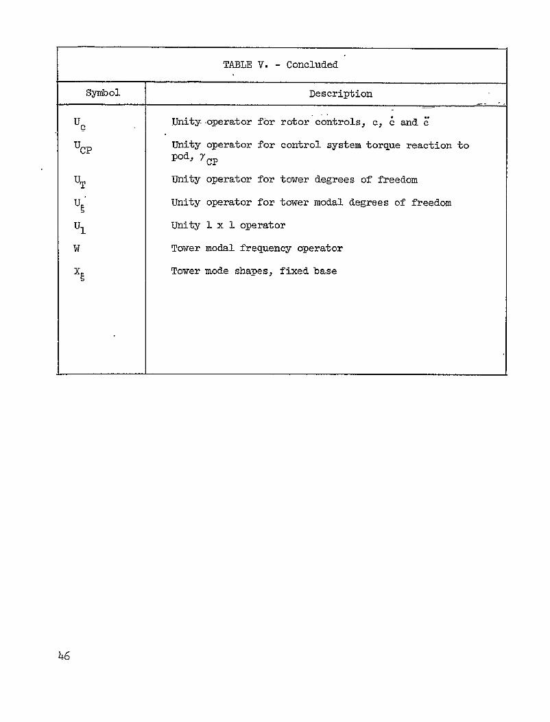
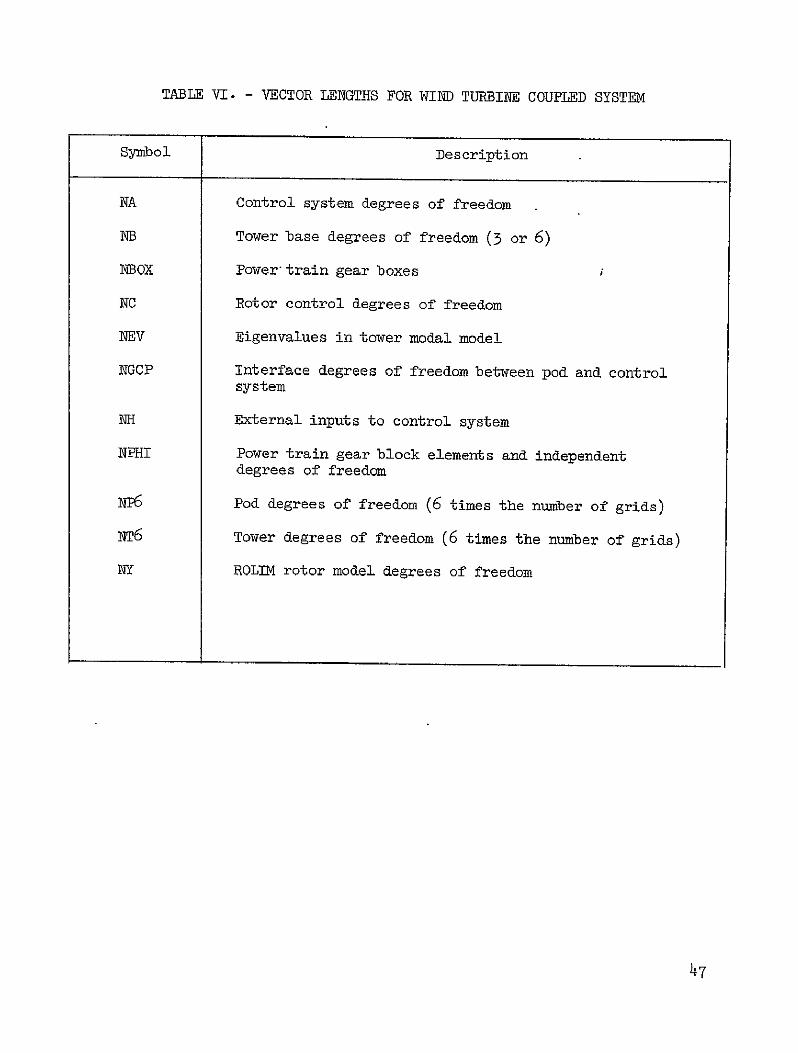
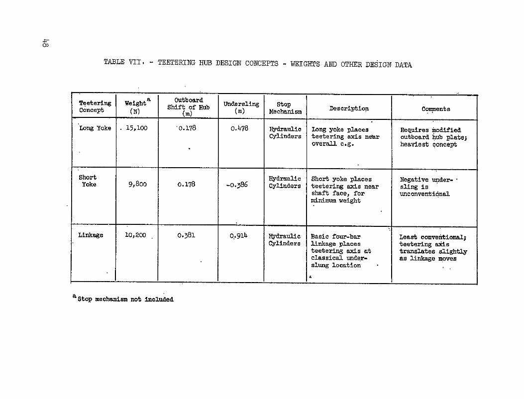
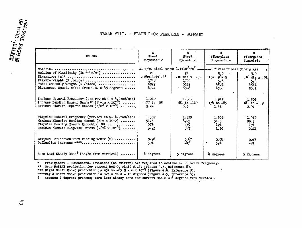
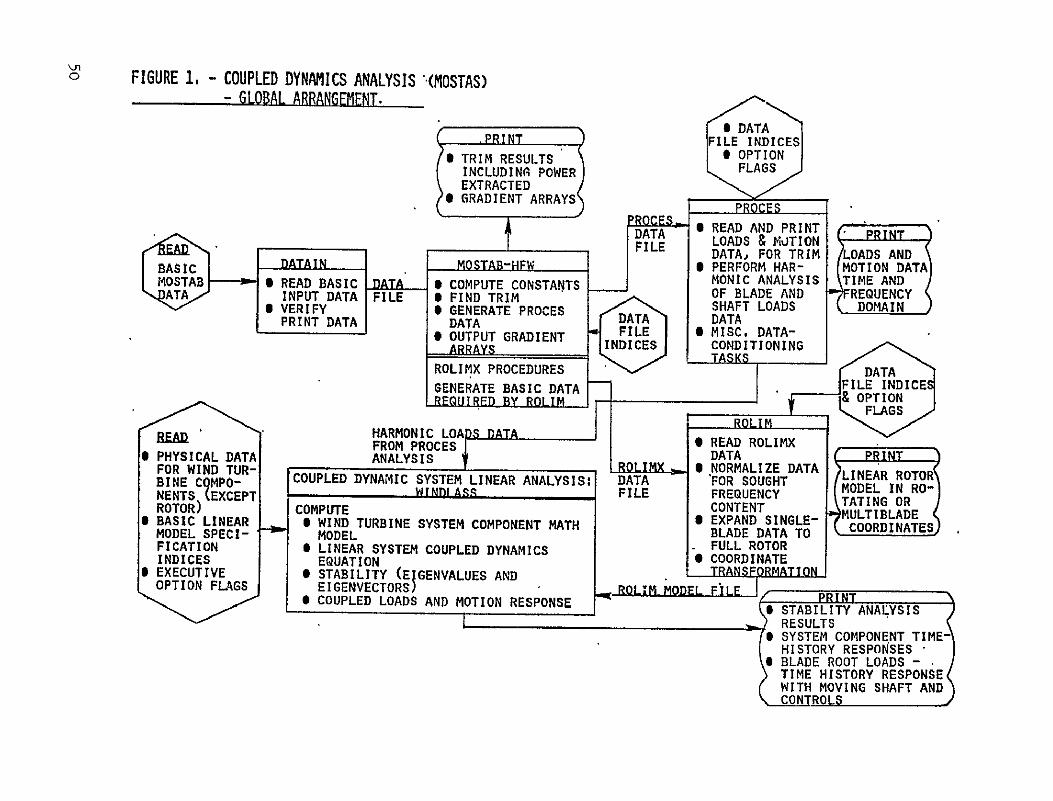
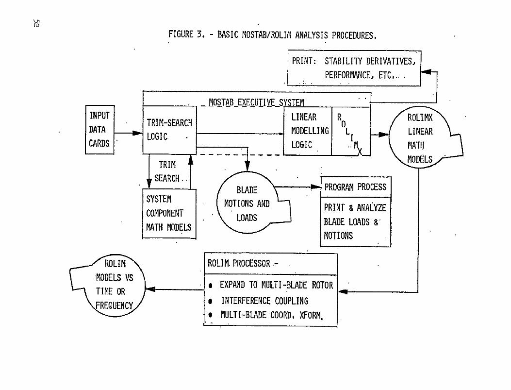
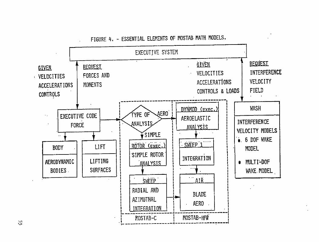
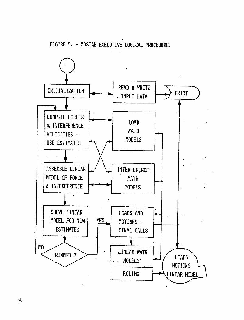
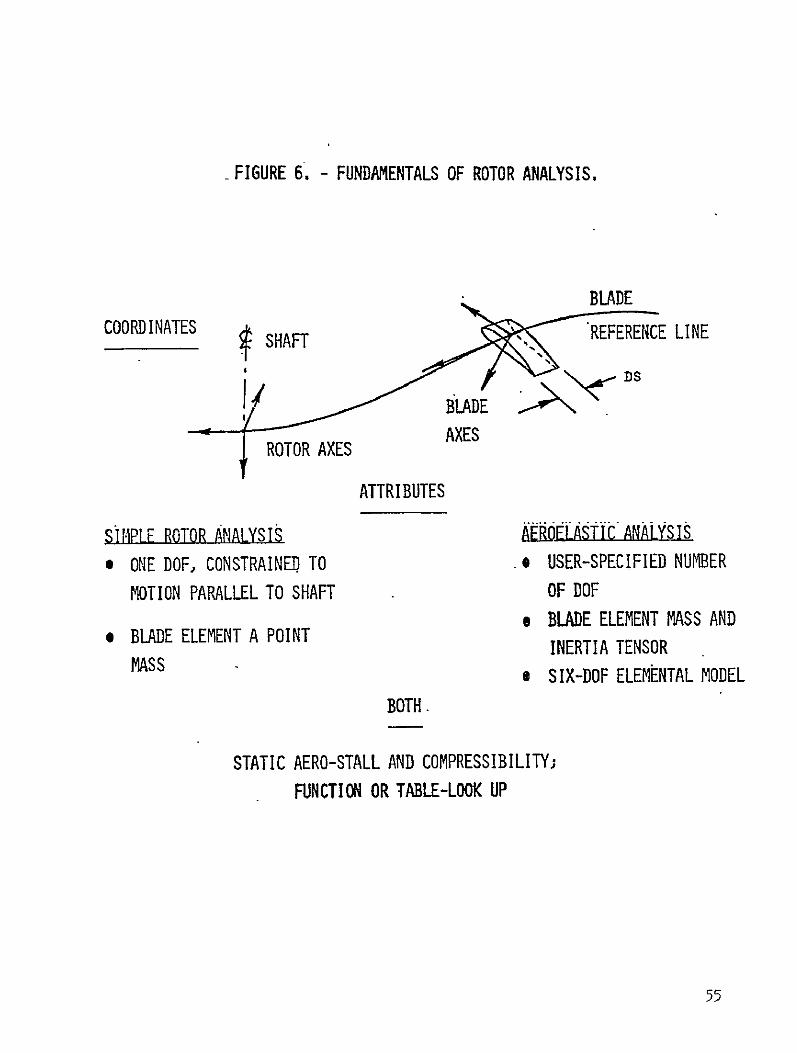
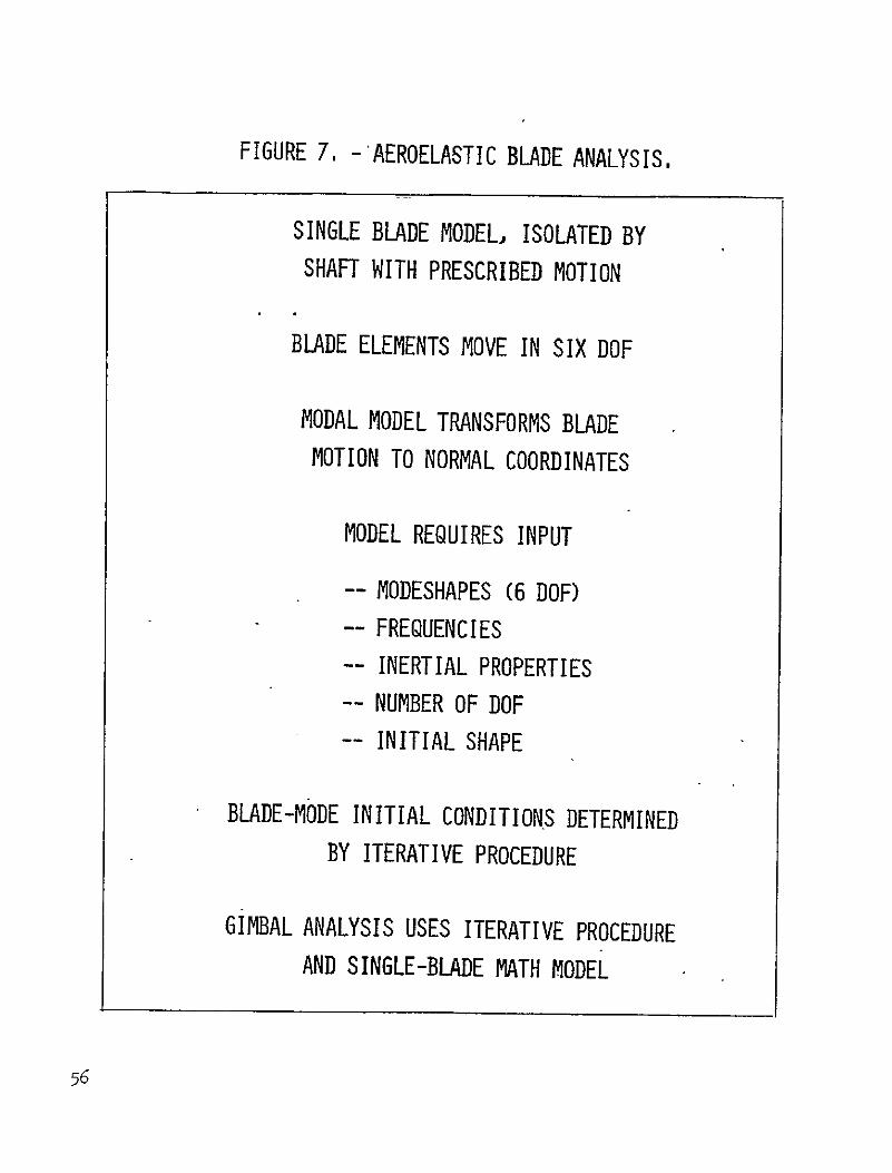
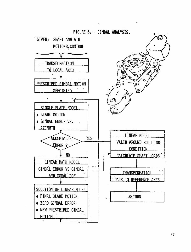
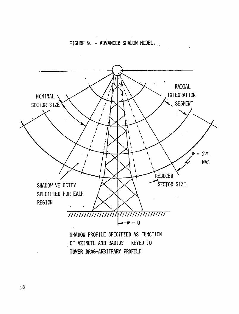
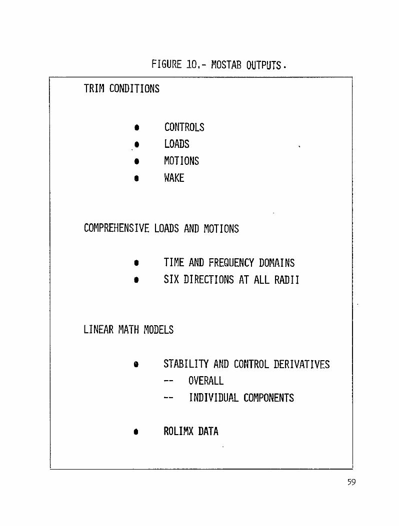
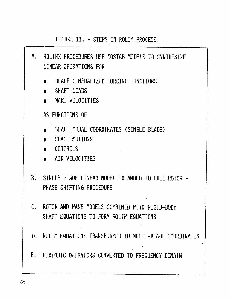
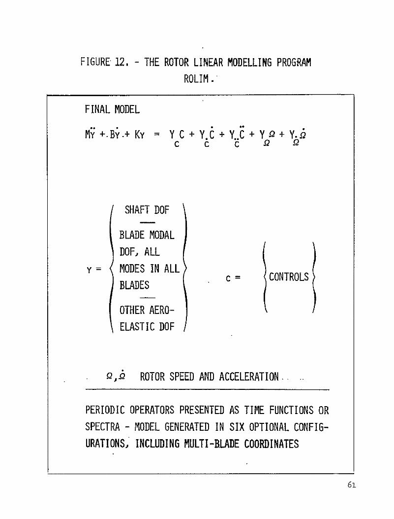
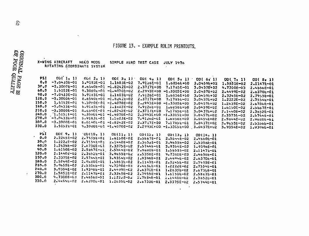
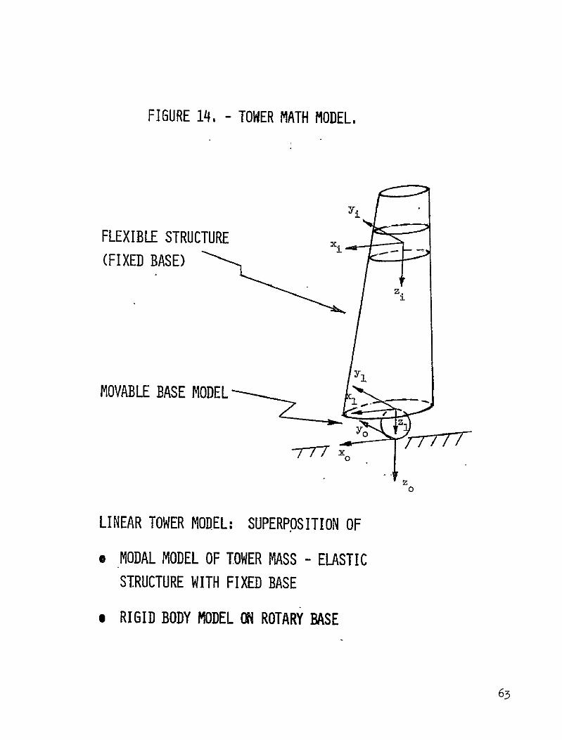
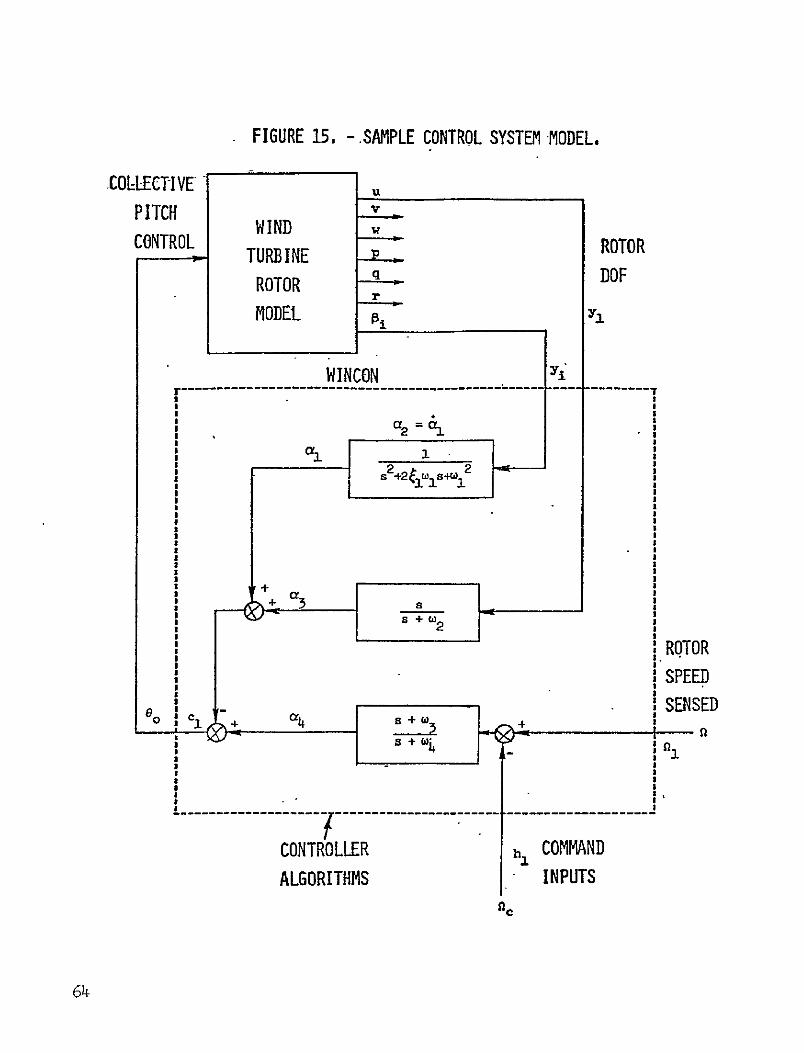
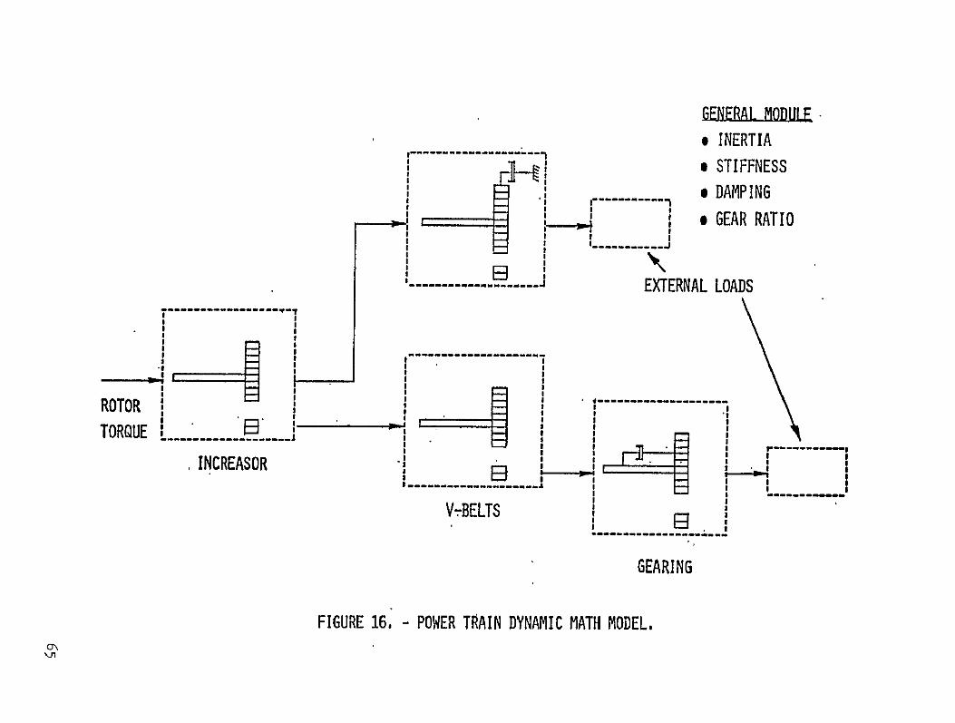
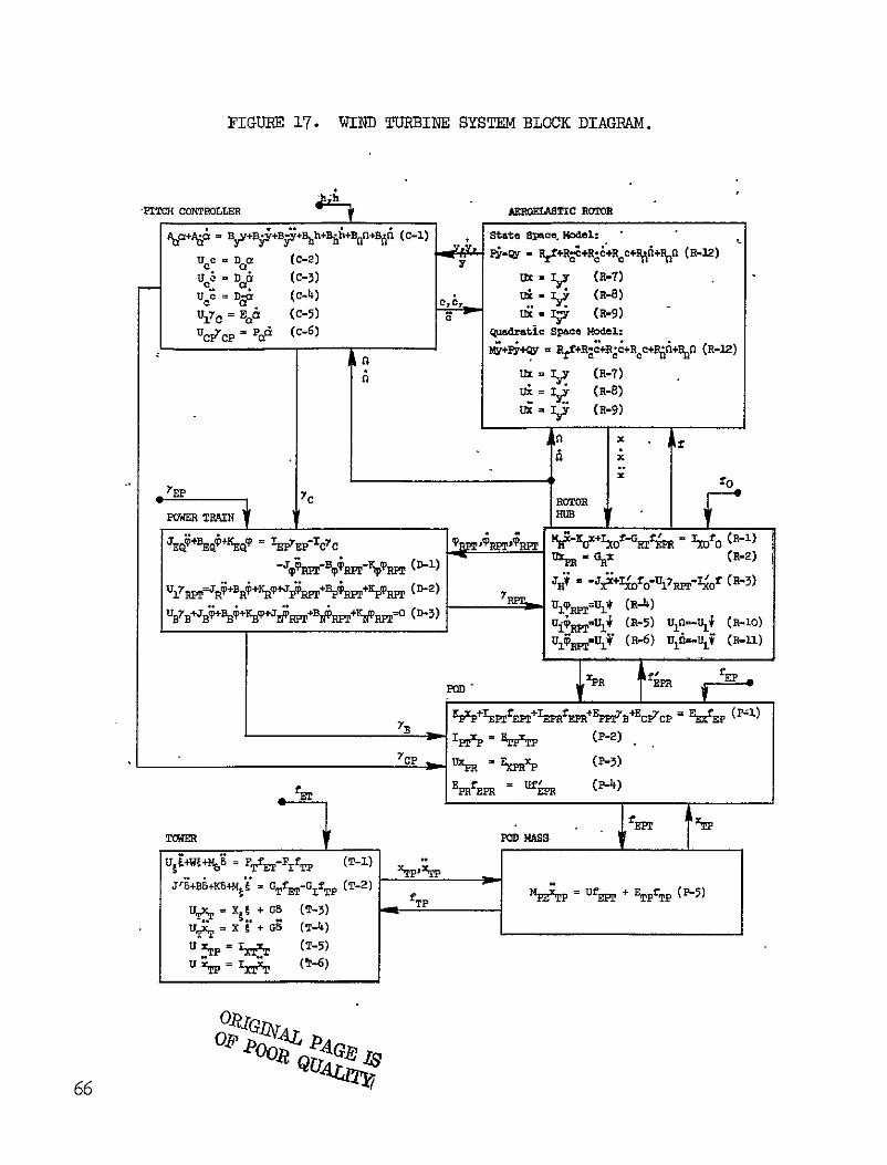
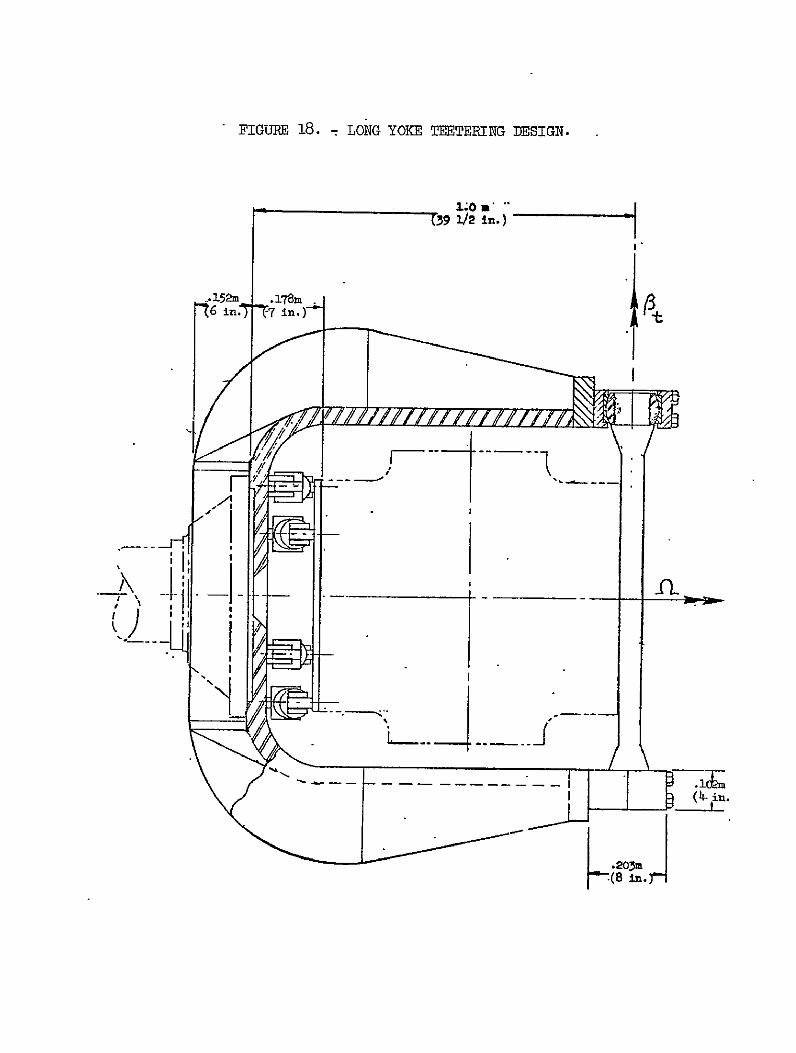
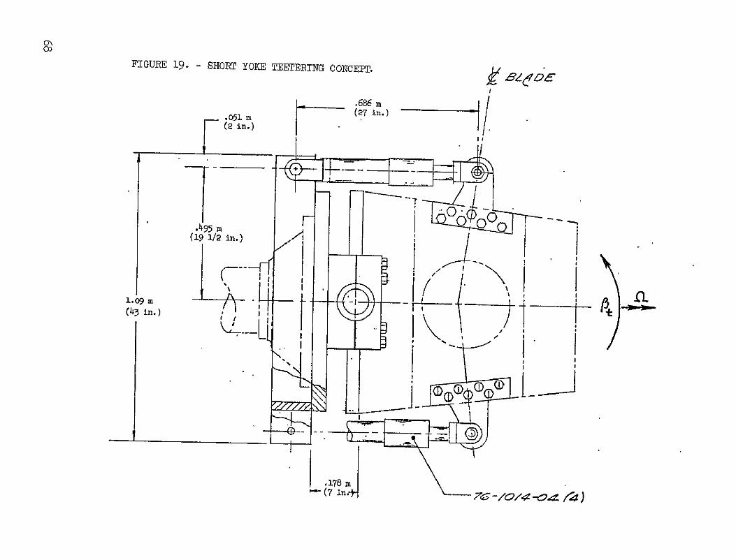
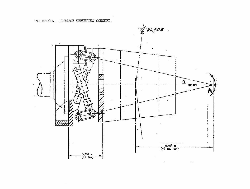
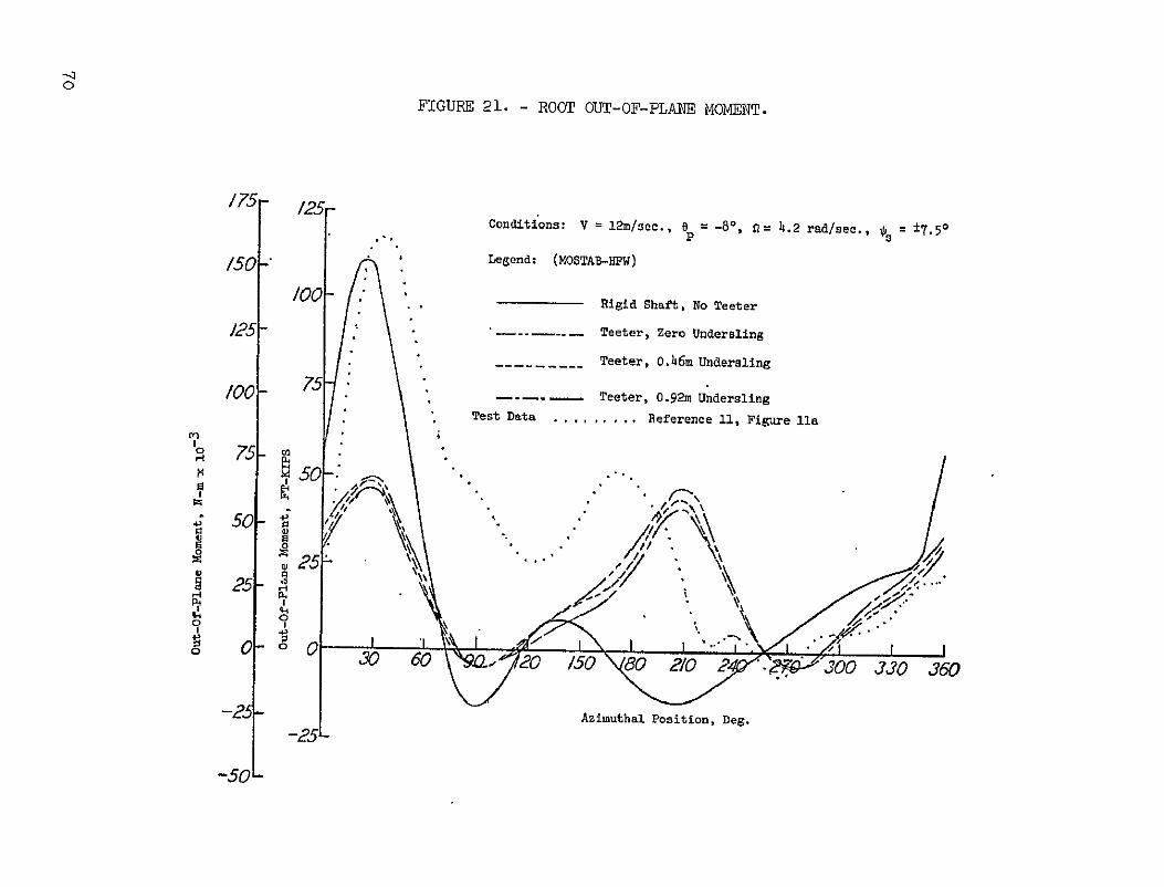
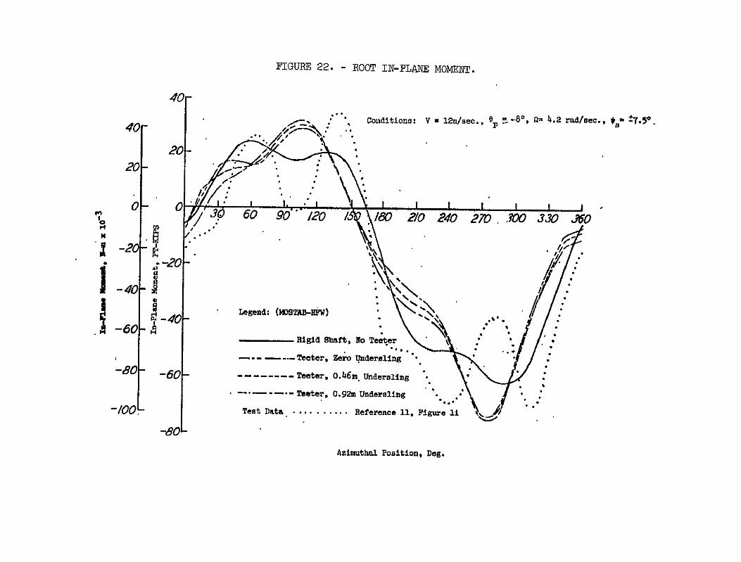
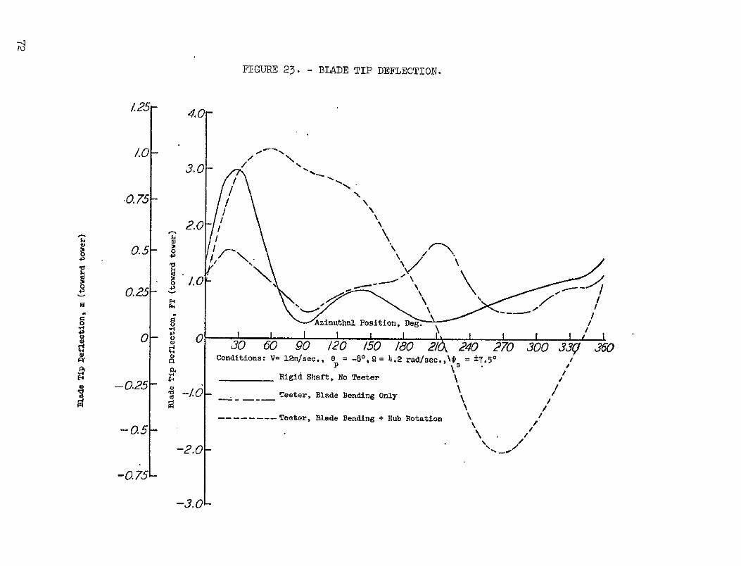
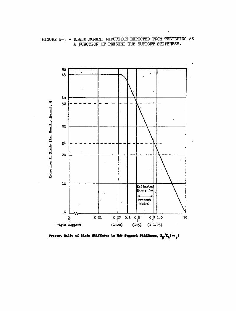
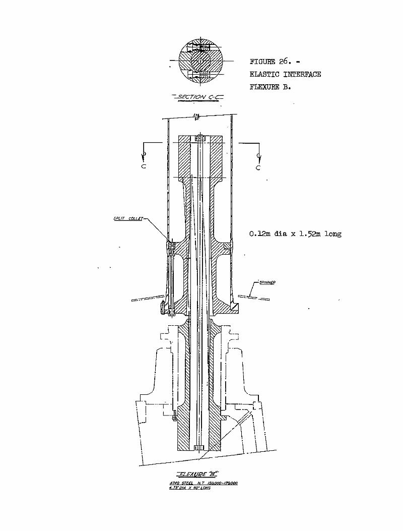
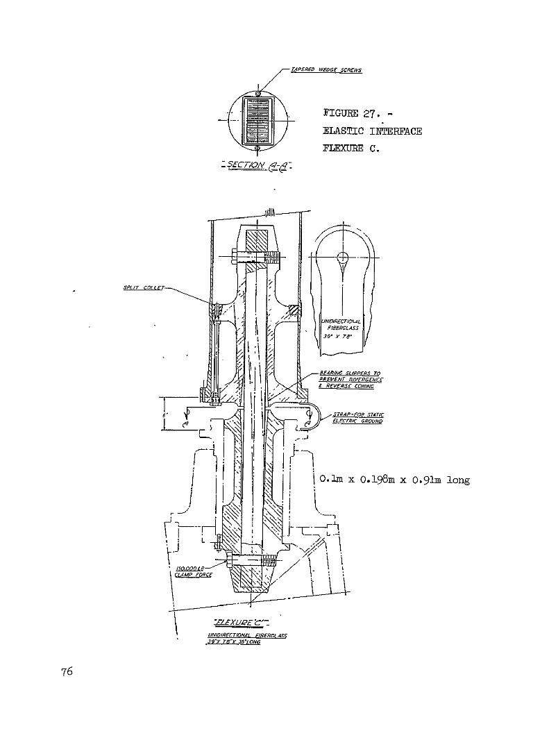
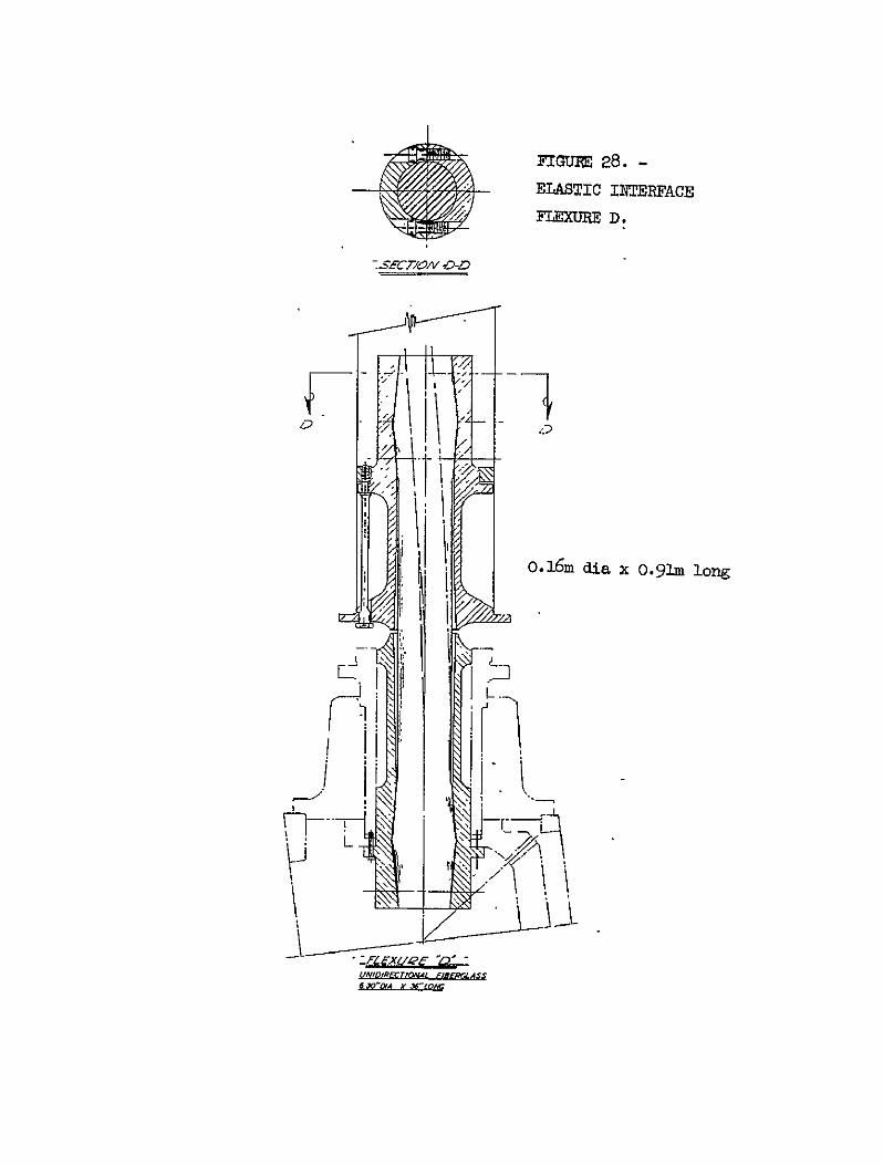
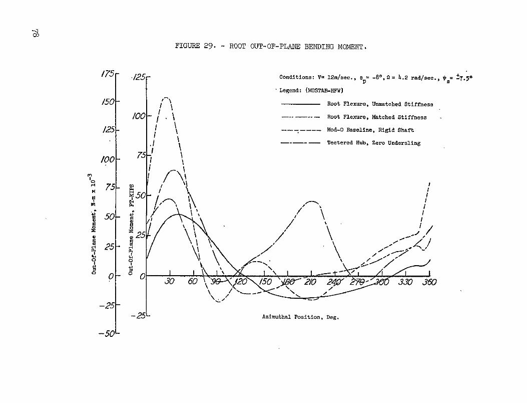
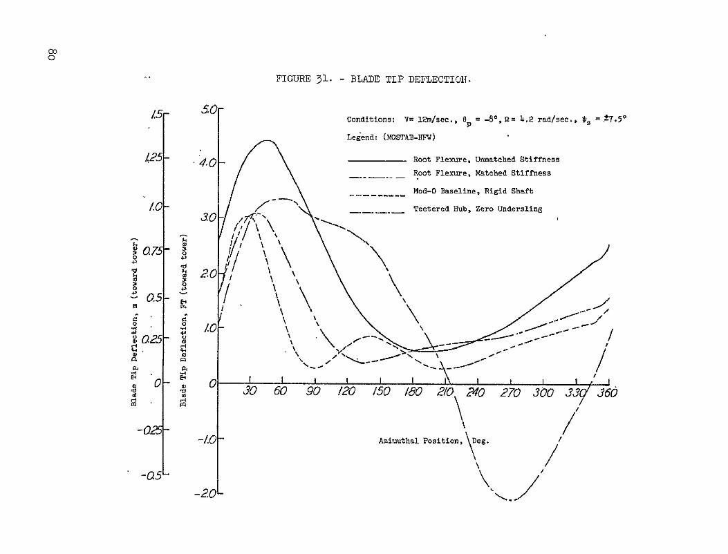