AoPS: Introduction to Counting & Probability. Chapter 1 Counting is Arithmetic.

Counting simple knots
via arithmetic invariants
Alison Beth Miller
A Dissertation
Presented to the Faculty
of Princeton University
in Candidacy for the Degree
of Doctor of Philosophy
Recommended for Acceptance
by the Department of
Mathematics
Adviser: Manjul Bhargava
September 2014

c© Copyright by Alison Beth Miller, 2014.
All rights reserved.

Abstract
Knot theory and arithmetic invariant theory are two fields of mathematics that
rely on algebraic invariants. We investigate the connections between the two, and
give a framework for addressing asymptotic counting questions relating to knots and
knot invariants.
We study invariants of simple (2q − 1)-knots when q is odd; these include the
Alexander module and Blanchfield pairing. In the case that q = 1, simple 1-knots are
exactly knots as classically defined. In the high-dimensional cases of q ≥ 3, the theory
is different, and simple knots are exactly classified by these algebraic invariants.
These invariants connect to arithmetic invariant theory by way of the theory
of Seifert matrices, which are related to the Z-orbits of the adjoint representation
Sym2(2g) of the algebraic group Sp2g. We classify the orbits of this representation
over general fields and over Z. These techniques are modeled after those of Bhargava,
Gross, and Wood in arithmetic invariant theory, but also have much in common with
methods used by Trotter and others in the topological context. We explain how our
results fit into this topological context of the Alexander module, Blanchfield pairing,
and related invariants.
In the final section, we look at how this connection can be used to asymptotically
count simple knots and Seifert hypersurfaces ordered by the size of their Alexander
polynomial. For knots of genus 1, the theory of binary quadratic forms yields an
explicit count for Seifert surfaces. We also conjecture heuristics for the asymptotic
number of genus 1 knots. These heuristics imply that most such knots have Alexander
polynomial of the form pt2 + (1− 2p)t+ p where p is a positive prime number. Using
sieve methods, we obtain an upper bound for the asymptotic count of such knots that
agrees with our heuristics.
iii

Acknowledgements
I would like to thank the many people who helped make this possible. First of
all, my advisor, Manjul Bhargava, for his support, encouragement, and enthusiasm
throughout my time in graduate school, as well as for a fascinating thesis topic. I
thank Benedict Gross, Peter Ozsvath, Jack Thorne, and Zoltan Szabo for helpful
conversations, Lenny Ng for providing feedback on drafts, and Peter Ozsvath for
agreeing to be a thesis reader. I additionally thank Catherine Miller and Aaron
Pixton for help with proofreading.
I would like to thank Princeton University and the NSF and NDSEG graduate
fellowships for providing financial support throughout graduate school. I thank the
Princeton Math Department for providing an intellectual home for me for five years.
My fellow math graduate students, housemates, and other friends have provided
invaluable companionship and moral support to me while in graduate school. Among
them, I must particularly thank Yaim Cooper, Heather Macbeth, and Aaron Pixton.
Finally I would like to thank my parents, Mary O’Keeffe and Ross Miller, and my
sister, Catherine Miller, who understand both how wonderful and how difficult both
mathematics and writing can be, and who have been with me all the way through.
Although my father did not live to see this thesis completed, he continues to be an
inspiration.
iv

To Ross Miller (1954-2013)
v

Contents
Abstract . . . . . . . . . . . . . . . . . . . . . . . . . . . . . . . . . . . . . iii
Acknowledgements . . . . . . . . . . . . . . . . . . . . . . . . . . . . . . . iv
1 Introduction 1
1.1 Historical background . . . . . . . . . . . . . . . . . . . . . . . . . . . 2
1.2 Outline . . . . . . . . . . . . . . . . . . . . . . . . . . . . . . . . . . . 4
2 Background on n-knots 6
2.1 Basic concepts and definitions in the theory of n-knots . . . . . . . . 6
2.2 The classification of simple Seifert hypersurfaces by Sp2g-orbits . . . . 10
2.3 The classification of simple knots . . . . . . . . . . . . . . . . . . . . 15
3 The arithmetic of Sp2g-orbits on 2g × 2g symmetric matrices 17
3.1 The orbits over an algebraically closed field and algebraic invariants . 17
3.2 The orbits over a general field . . . . . . . . . . . . . . . . . . . . . . 19
3.3 The orbits over Z . . . . . . . . . . . . . . . . . . . . . . . . . . . . . 25
4 Connections to the Alexander module and related knot invariants 31
4.1 The Alexander polynomial . . . . . . . . . . . . . . . . . . . . . . . . 32
4.2 Conjugate-self-balanced O∆-modules . . . . . . . . . . . . . . . . . . 34
4.3 The Alexander module as a conjugate-self-balanced module . . . . . . 36
4.3.1 Comparing conjugate-self-balanced modules . . . . . . . . . . 36
vi

4.3.2 Conjugate-self-balanced ideal classes of Dedekind rings . . . . 41
5 Counting 42
5.1 Finiteness theorems for Seifert hypersurfaces and simple knots . . . . 42
5.2 Strategies . . . . . . . . . . . . . . . . . . . . . . . . . . . . . . . . . 44
5.3 Counting genus 1 Seifert hypersurfaces . . . . . . . . . . . . . . . . . 46
5.3.1 2×2 Seifert-parity symmetric matrices, binary quadratic forms,
and ideals in quadratic rings . . . . . . . . . . . . . . . . . . . 46
5.3.2 Counting Seifert forms of negative discriminant . . . . . . . . 47
5.3.3 Counting Seifert forms of positive discriminant . . . . . . . . . 53
5.4 Counting genus 1 simple knots . . . . . . . . . . . . . . . . . . . . . . 53
5.4.1 The map ι∗ . . . . . . . . . . . . . . . . . . . . . . . . . . . . 53
5.4.2 A sieving argument . . . . . . . . . . . . . . . . . . . . . . . . 57
5.4.3 Heuristics . . . . . . . . . . . . . . . . . . . . . . . . . . . . . 60
Bibliography 61
vii

Chapter 1
Introduction
In this thesis, we will explore a connection between two separate branches of math-
ematics: arithmetic invariant theory and knot theory. This connection comes about
by way of knot invariants that have natural arithmetic structure. We will consider
the question of counting these arithmetic objects, and the consequences for counting
high-dimensional simple knots.
Arithmetic invariant theory, a term coined by Bhargava and Gross in [3], deals
with the questions of the following form. Suppose G is an algebraic matrix group
defined over a ring R, and V is a finite-dimensional representation of G. What are
the orbits of G(R) acting on V (R)? What sorts of invariants classify them? This
is a well-studied problem when R is an algebraically closed field, in which case the
invariants are always polynomial functions on V ; however, if R is non-algebraically
closed field, or a general ring, there is additional arithmetic complexity.
The goal of knot theory is different: to understand the topologically distinct ways
that one manifold can be embedded into another. Classical knots are embedded
circles in S3, but knots can also be defined in higher dimensions: an n-knot is an
embedding of Sn in Sn+2. Knot theory also concerns itself with invariants; there are
1
many ways to construct invariants of knots. However, it is in general much harder to
completely classify knots by their invariants.
Some knot invariants, in particular those related to the Alexander module and
to the Seifert pairing, have natural arithmetic structure; they can be thought of as
ideal classes of rings, or as Z-orbits of a representation of Sp2g. These structures were
analyzed by a number of knot theorists, including Milnor [25] and Trotter[30]. The
arguments they made were of a similar nature to ones made in work by Bhargava and
Gross [3] and of Wood [32]. In Chapter 3, we will reinterpret their arguments in the
context of arithmetic invariant theory.
The bijections given by arithmetic invariant theory have made it possible to count
a wide range of objects, including points on elliptic curves, finite dimensional Z-
algebras, and ideal classes of orders in number fields. In this thesis, using the con-
nection between arithmetic invariant theory and algebraic knot invariants, we will
extend the range of these techniques to count high-dimensional knots as well.
1.1 Historical background
Historically, the first researchers to look at algebraic-number-theoretic invariants of
knots were Fox and Smythe [12], studying classical knots in S3. Their construction
implicitly used the Alexander module via a presentation matrix. Hillman [13] later
recast their work in terms of module theory and simultaneously generalized the results
to links in S3. Many of the results from that paper are recapitulated in [14]. The
generalization to links meant that Hillman worked with Laurent polynomial rings in
more variables, which we shall not be concerned with.
At the same time, Kearton, Levine, and others were developing the general higher-
dimensional theory of n-knots, that is, knotted copies of Sn in Sn+2.
2

(Some parts of the theory of higher-dimensional knots also have similar algebraic
structures: see [21] and [14] for more details.)
Meanwhile, the Alexander module had been studied as an object in its own right.
One thing that was realized early on was that the Alexander module had additional
structure; in fact it was endowed with a canonical pairing, known as the Blanch-
field pairing (introduced by Blanchfield [7]). Knot theorists studied properties of the
Alexander module, and also worked on the question of classifying the possible mod-
ules that could be realized as Alexander modules of some knot. Most of the work
done involved higher-dimensional generalizations.
When n = 2q−1 is odd, one productive way to understand the Alexander module
of an n-knot K is to choose an embedded hypersurface V in Sn+2 with boundary
equal to K. The homology group Hq(V,Z) then carries a natural non-symmetric
Z-valued pairing, known as the “Seifert pairing” such that the skew-symmetric part
of the Seifert pairing is the intersection pairing on S. The Seifert pairing is not an
invariant of the knot K, but depends upon the hypersurface V . For one thing, the
rank of the homology group H1(V,Z) depends upon the choice of V , but even if one
fixes the rank the isomorphism class of Seifert pairing can still depend on the choice
of V . In order to construct a true invariant one must impose a weaker equivalence
relation called “S-equivalence” on matrices, which has the property that any two
Seifert matrices for the same knot are S-equivalent.
The relevance of Seifert pairings for us is that knowing a Seifert matrix for a knot
is sufficient information to compute the Alexander module along with its Blanchfield
pairing. In fact (as shown, e.g., by Trotter [29]), two knots have isomorphic Alexander
modules and Blanchfield pairings if and only if they have Seifert matrices that are
S-equivalent. Therefore, one approach to finding number-theoretic invariants of knots
is to look for invariants of the Seifert pairing (here considered as a pairing on a free Z-
3
module, not as an S-equivalence class) and then to determine which of them become
knot invariants.
Another feature of the Seifert pairing is that it is easy to construct matrices with
desired Seifert pairing. For this reason, the Seifert matrix approach was used to study
the realization problem for Alexander modules. In particular, it was used by Trotter
[30] who built on previous work of Levine [20], to give an algebraic criterion for which
Z[t, t−1]-modules are middle-dimensional Alexander modules.
Although in general these invariants are not complete invariants, there is one
important class of knots for which they are. These are the simple n-knots, those
whose complement has the homotopy type of a circle up until the middle dimension.
Simple n-knots are fully classified by their Alexander module and Blanchfield pairing.
They were introduced by Levine [19], and classified in multiple equivalent ways by
Levine [19], Kearton [17], and Farber [10].
Using this classification, Bayer and Michel [1] proved that there are only finitely
many equivalence classes of simple knots with a fixed squarefree Alexander polyno-
mial. They also proved a similar theorem for simple Seifert hypersurfaces.
1.2 Outline
This thesis has two main goals. The first is to revisit the knot invariants described
above from the point of view of arithmetic invariant theory. The second is to explore
the new question of finding asymptotics for the number of simple (2q− 1)-knots with
Alexander polynomials of bounded height. By the result of Bayer and Michel [1],
we know this number is finite: an answer to this question thus gives an average-case
quantitative version of their results.
Chapter 2 covers background material from high-dimensional knot theory. In
Chapter 3 we consider the question of the Sp2g(R) orbits on 2g × 2g Seifert matrices
4

in the cases where R is a field or R = Z. This is an arithmetic question that arises
naturally from the topological question of the classification of Seifert hypersurfaces,
and which has been studied extensively by topologists for that reason. We study it
from the point of view of arithmetic invariant theory, and explain the connection to
previous work done by topologists on the question.
Chapter 4 explains the connection between the arithmetic invariants from Chap-
ter 2 and knot invariants related to the Alexander polynomial.
Chapter 5 deals with the question of counting simple knots and simple Seifert
hypersurfaces. We prove asymptotics for counting simple Seifert hypersurfaces of
genus 1, and give heuristics, based on standard conjectures in number theory, for the
asymptotics of the number of simple knots of genus 1. In particular, we conjecture that
most simple knots of genus 1 have Alexander polynomials of the form pt2+(1−2p)t+p.
We use sieve theory to prove an upper bound for the number of knots with Alexander
polynomial of that form.
5

Chapter 2
Background on n-knots
2.1 Basic concepts and definitions in the theory of
n-knots
We are interested in counting n-knots by way of invariants with interesting arithmetic
structure. Informally, an n-knot is a knotted copy of Sn in Sn+2. There are multiple
ways of making this rigorous; the following two definitions are both commonly used:
Definition.
(i) An n-knot K is a topologically embedded copy of Sn in Sn+2 that is locally flat
(locally homeomorphic to Rn ⊂ Rn+2). Equivalence is given by ambient isotopy.
(ii) An n-knot is a smoothly embedded submanifold K of Sn+2 which is homeomor-
phic to Sn (but not necessarily diffeomorphic; K might be an exotic sphere).
Equivalence is induced by orientation-preserving diffeomorphism of the Sn+2.
In both cases, we will consider both Sn and Sn+2 to be oriented, so that reversing
the orientation of either or both may give a different knot.
Although it is far from obvious, classification results we use will give the same
answer regardless of which of the two definitions above is used. I will talk about
6
knots and equivalence with the understanding that all statements hold using either
formulation.
We will be interested in the following class of n-knots, which has a nice classifica-
tion.
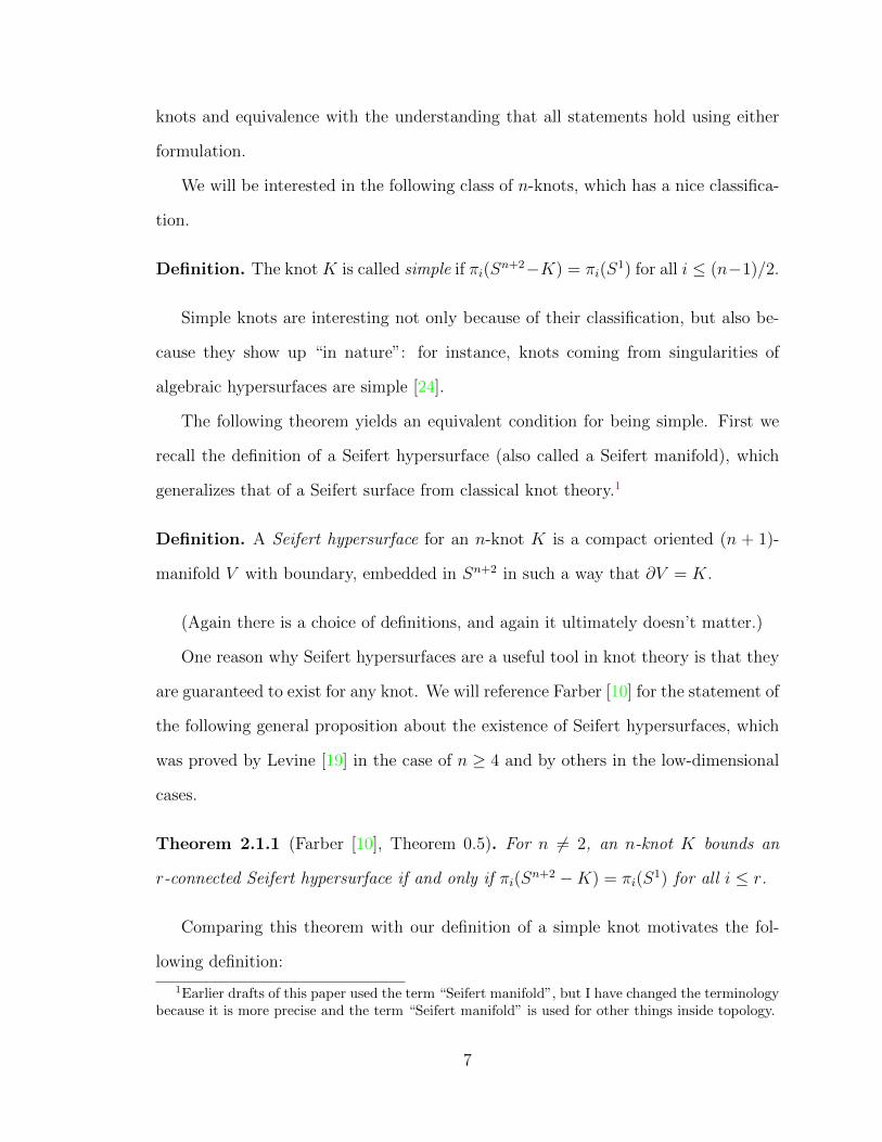
Definition. The knot K is called simple if πi(Sn+2−K) = πi(S
1) for all i ≤ (n−1)/2.
Simple knots are interesting not only because of their classification, but also be-
cause they show up “in nature”: for instance, knots coming from singularities of
algebraic hypersurfaces are simple [24].
The following theorem yields an equivalent condition for being simple. First we
recall the definition of a Seifert hypersurface (also called a Seifert manifold), which
generalizes that of a Seifert surface from classical knot theory.1
Definition. A Seifert hypersurface for an n-knot K is a compact oriented (n + 1)-
manifold V with boundary, embedded in Sn+2 in such a way that ∂V = K.
(Again there is a choice of definitions, and again it ultimately doesn’t matter.)
One reason why Seifert hypersurfaces are a useful tool in knot theory is that they
are guaranteed to exist for any knot. We will reference Farber [10] for the statement of
the following general proposition about the existence of Seifert hypersurfaces, which
was proved by Levine [19] in the case of n ≥ 4 and by others in the low-dimensional
cases.
Theorem 2.1.1 (Farber [10], Theorem 0.5). For n 6= 2, an n-knot K bounds an
r-connected Seifert hypersurface if and only if πi(Sn+2 −K) = πi(S
1) for all i ≤ r.
Comparing this theorem with our definition of a simple knot motivates the fol-
lowing definition:
1Earlier drafts of this paper used the term “Seifert manifold”, but I have changed the terminologybecause it is more precise and the term “Seifert manifold” is used for other things inside topology.
7
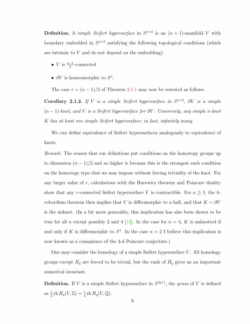
Definition. A simple Seifert hypersurface in Sn+2 is an (n + 1)-manifold V with
boundary embedded in Sn+2 satisfying the following topological conditions (which
are intrinsic to V and do not depend on the embedding):
• V is n−12
-connected
• ∂V is homeomorphic to Sn.
The case r = (n− 1)/2 of Theorem 2.1.1 may now be restated as follows.
Corollary 2.1.2. If V is a simple Seifert hypersurface in Sn+2, ∂V is a simple
(n− 1)-knot, and V is a Seifert hypersurface for ∂V . Conversely, any simple n-knot
K has at least one simple Seifert hypersurface; in fact, infinitely many.
We can define equivalence of Seifert hypersurfaces analogously to equivalence of
knots.
Remark. The reason that our definitions put conditions on the homotopy groups up
to dimension (n− 1)/2 and no higher is because this is the strongest such condition
on the homotopy type that we may impose without forcing triviality of the knot. For
any larger value of r, calculations with the Hurewicz theorem and Poincare duality
show that any r-connected Seifert hypersurface V is contractible. For n ≥ 5, the h-
cobordism theorem then implies that V is diffeomorphic to a ball, and that K = ∂V
is the unknot. (In a bit more generality, this implication has also been shown to be
true for all n except possibly 2 and 4 [10]. In the case for n = 4, K is unknotted if
and only if K is diffeomorphic to S4. In the case n = 2 I believe this implication is
now known as a consquence of the 3-d Poincare conjecture.)
One may consider the homology of a simple Seifert hypersurface V . All homology
groups except Hq are forced to be trivial, but the rank of Hq gives us an important
numerical invariant.
Definition. If V is a simple Seifert hypersurface in S2q+1, the genus of V is defined
as 12
rkHq(V,Z) = 12
rkHq(V,Q).
8

This definition always yields a whole number, because Hq(V,Z) has a nondegen-
erate skew-symmetric pairing (the intersection pairing).
We can also define the genus of a knot. This is more complicated, because the
homology of the knot complement does not give us any information. Indeed, the
complement S2q+1 −K of a simple knot always has the same homology as S1.
However, because H1(S2q+1 −K) ∼= Z, there is a unique covering space (S2q+1 −
K)cyc of S2q+1 −K with infinite cyclic covering group.
We can then define the genus of a knot intrinsically.
Definition. Let K be a simple knot in S2q+1 with q ≥ 3. We define the genus of K
as 12
rkHq((S2q+1 −K)cyc,Q).
Theorem 2.1.3. Let K be a simple knot in S2q+1, with q ≥ 3. Then genus(K) is
always finite, an integer, and equal to min(genus(V )) where V ranges over all simple
Seifert hypersurfaces such that ∂V = K.
Proof. This follows from the existence of minimal Seifert hypersurfaces, as proved in
[11].
Remark. In the theory of classical knots in S3, the genus is typically defined as the
minimum genus of a Seifert surface. We choose the equivalent definition in terms of
the infinite cyclic cover here because it is simpler to state.
The homology group Hq((S2q+1−K)cyc) will also be important to us as an object
in its own right, because it is an Alexander module for K. We will refer to it as
“the Alexander module of K”, because the Alexander modules coming from the ith
homology when i 6= q turn out to be all trivial.
We now go into detail regarding this definition.
Let t be a generator of the group of deck transformations of (S2q+1 − K)cyc:
using the orientations on K and on S2q+1, we can make a canonical choice of t.
9

The group of deck transformations acts on Hq((S2q+1 − K)cyc,Z), and thus makes
Hq((S2q+1 −K)cyc,Z) into a module over the group ring Z[t, t−1].
Definition. The Alexander module AlexK of a knot K is the Z[t, t−1]-module
Hq((S2q+1 −K)cyc,Z).
The Alexander module also possesses an important duality pairing, known as the
Blanchfield pairing. We will not get into the details of its construction here, but we
will state its existence.
Theorem 2.1.4 (Blanchfield, [7]). There is a canonical perfect pairing, the Blanch-
field pairing
Bl : AlexK × AlexK → Q(t)/(Z[t, t−1]),
which is Hermitian with respect to the involution of Z[t, t−1] interchanging t with t−1.
2.2 The classification of simple Seifert hypersur-
faces by Sp2g-orbits
The remainder of this chapter will be dedicated to the classifications of simple Seifert
hypersurfaces and of simple knots by algebraic data. We will follow the standard
expository path due to Kearton, Levine, Trotter, and Farber, which starts with the
classification of Seifert hypersurfaces and then passes to knots.
As before, we will study simple knots of genus g inside S2q+1, where g and q are
fixed, and q is at least 3. The results below will depend on the choice of g, but will
be independent of q.
We first consider simple Seifert hypersurfaces inside S2q+1. If V is a simple
Seifert hypersurface, the homology group Hq(V,Z) posseses a natural Z-valued skew-
10
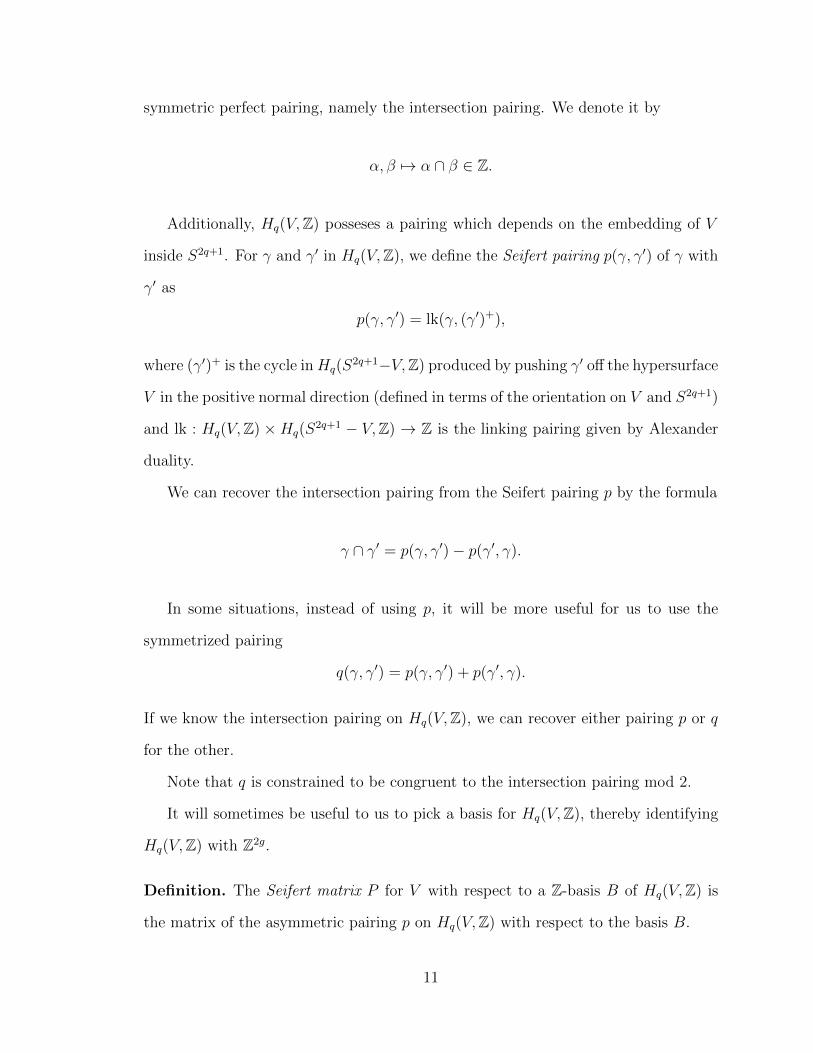
symmetric perfect pairing, namely the intersection pairing. We denote it by
α, β 7→ α ∩ β ∈ Z.
Additionally, Hq(V,Z) posseses a pairing which depends on the embedding of V
inside S2q+1. For γ and γ′ in Hq(V,Z), we define the Seifert pairing p(γ, γ′) of γ with
γ′ as
p(γ, γ′) = lk(γ, (γ′)+),
where (γ′)+ is the cycle inHq(S2q+1−V,Z) produced by pushing γ′ off the hypersurface
V in the positive normal direction (defined in terms of the orientation on V and S2q+1)
and lk : Hq(V,Z) ×Hq(S2q+1 − V,Z) → Z is the linking pairing given by Alexander
duality.
We can recover the intersection pairing from the Seifert pairing p by the formula
γ ∩ γ′ = p(γ, γ′)− p(γ′, γ).
In some situations, instead of using p, it will be more useful for us to use the
symmetrized pairing
q(γ, γ′) = p(γ, γ′) + p(γ′, γ).
If we know the intersection pairing on Hq(V,Z), we can recover either pairing p or q
for the other.
Note that q is constrained to be congruent to the intersection pairing mod 2.
It will sometimes be useful to us to pick a basis for Hq(V,Z), thereby identifying
Hq(V,Z) with Z2g.
Definition. The Seifert matrix P for V with respect to a Z-basis B of Hq(V,Z) is
the matrix of the asymmetric pairing p on Hq(V,Z) with respect to the basis B.
11

Because the intersection pairing is a perfect pairing, any Seifert matrix P must
satisfy det(P −P T ) = 1. We will see later that this condition is sufficient for a matrix
P to be a Seifert matrix of some Seifert hypersurface.
Another consequence of the intersection pairing being a perfect pairing is that we
can, if we wish, choose a basis of Hq(V,Z) in which the intersection pairing is identified
with the standard symplectic pairing 〈v, w〉 = vTJw on Z2g, where J = Jg =(
0 Ig−Ig 0
).
In this setting, the parity condition on the quadratic form q and on its associated
matrix Q motivates the following definition:
Definition. We say that a symmetric bilinear form m on Z2g is Seifert-parity if
m(x, y) ≡ 〈x, y〉 (mod 2) for all x, y ∈ Z2g.
We say that a symmetric 2g × 2g matrix Q is Seifert-parity if Q is the matrix of a
Seifert-parity symmetric bilinear form, or equivalently,
Q ≡ J (mod 2).
(Note that the Seifert-parity condition is a condition on the parity on the sym-
metric matrix Q, not on the Seifert matrix itself!)
First we introduce some algebraic preliminaries. Let Sp2g(Z) be the group of
integer matrices preserving the standard symplectic form 〈v, w〉 = vTJw on Z2g,
where J = Jg =(
0 Ig−Ig 0
).
In this way we can go from a simple Seifert hypersurface V to a 2g × 2g Seifert-
parity symmetric matrix Q.
The crucial topological fact is that one can also go in the other direction. The
following correspondence is due to Levine[19].
12

Theorem 2.2.1. If Q is a Seifert-parity symmetric 2g× 2g matrix, there is a unique
pair V, (α1, . . . , αg, β1, . . . , βg) with the properties that
(a) V is a simple Seifert hypersurface in S2q+1
(b) α1, . . . , αg, β1, . . . , βg constitute a basis for Hq(V,Z)
(c) αi ∩ αj = βi ∩ βj = 0, and αi ∩ βj = −βi ∩ αj = δij.
(d) the symmetrized pairing q(α, β) = p(α, β) + p(β, α) has matrix Q with respect
to the basis (α1, . . . , αg, β1, . . . , βg).
Very crude sketch. This fact is proved as part of the proof of Lemma 3 in [19]. We
provide a sketch of that proof here to show the basic details. We note that the last two
conditions listed may equivalently be stated as: the Seifert pairing p on Hq(V ) has
pairing matrix J+Q2
with respect to the basis (α1, . . . , αg, β1, . . . , βg). Define P = J+Q2
.
Start with a copy V0 of D2q inside S2q+1. We create V by attaching 2g different
handles to V0 along its boundary. Each handle is homeomorphic to Dq × Dq, and
is glued to V0 at the boundary by an attaching map Sq ×Dq → ∂V0. The resulting
manifold is (q − 1)-connected, and the handle decomposition yields an explicit basis
for Hq(V ;Z); each handle contributes one generator. By appropriately embedding
the handles in S2q+1, we can ensure that the Seifert pairing on Hq(V ;Z) has matrix
P . This gives us items (2) and (3); the one thing left to check is that ∂V is in
fact homeomorphic to S2q−1. It is a straightforward calculation (using the fact that
det J = 1) to check that the boundary ∂V has the same homology as S2q−1. As well,
∂V is simply-connected by construction (it has a cell decomposition using no 1-cells),
so ∂V is homeomorphic to S2q−1 by the (high-dimensional) Poincare conjecture.
To show uniqueness, one uses the fact from handlebody theory that any simple
Seifert hypersurface V has a handle decomposition of the type described above. The
only obstructions to deforming one such handle decomposition into another come
from the linking numbers of the handles, so V is unique up to isotopy.
13

Remark. In the classical theory of Seifert surfaces in S3, the construction above will
still produce Seifert manifolds with desired pairing. However, this construction is
very far from unique.
Theorem 2.2.1 can be restated as saying that there is a bijection between the set of
simple Seifert hypersurfaces with homology basis and the set of Seifert-parity 2g×2g
symmetric matrices. This can be stated more concisely using the following definition.
Definition. A symplectic basis for Hq(V,Z) is a basis B = (α1, . . . , αg, β1, . . . , βg) for
Hq(V,Z) such that αi ∩ αj = βi ∩ βj = 0 and αi ∩ βj = −βi ∩ αj = δij.
Corollary 2.2.2. There is a bijection
{simple Seifert hypersurfacesV of genus 2g equipped witha symplectic basis B forHq(V,Z)
} ⇔ { Seifert-parity 2g × 2g sym-metric matrices
}
given by sending the pair (V,B) to the matrix of the symmetric pairing q(γ, γ′)
with respect to the basis B.
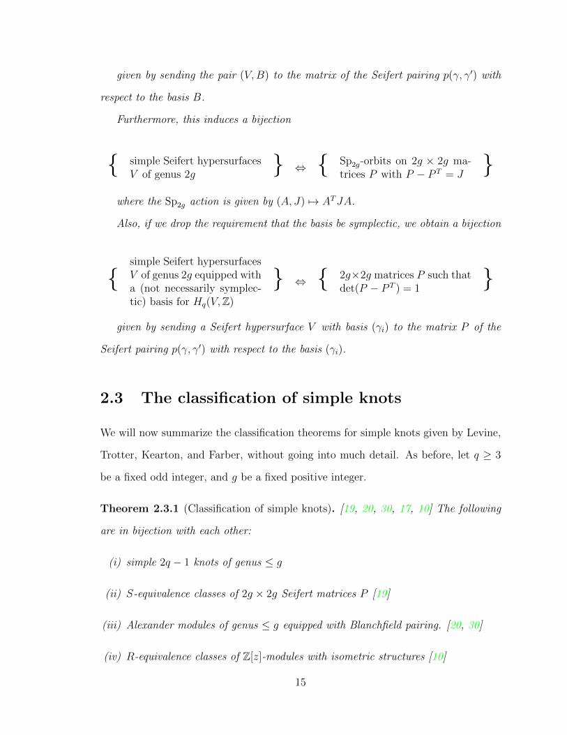
Furthermore, this induces a bijection
{ simple Seifert hypersurfacesV of genus 2g
} ⇔ { Sp2g(Z)-equivalence classesof Seifert-parity 2g × 2gsymmetric matrices
}where the Sp2g action is given by (A,Q) 7→ ATQA.
We can also state a version of this corollary using the Seifert matrix P of the
asymmetric pairing instead of Q.
Corollary 2.2.3. There is a bijection
{simple Seifert hypersurfacesV of genus 2g equipped witha symplectic basis B forHq(V,Z)
} ⇔ { 2g × 2g matrices P withP − P T = J
}14
given by sending the pair (V,B) to the matrix of the Seifert pairing p(γ, γ′) with
respect to the basis B.
Furthermore, this induces a bijection
{ simple Seifert hypersurfacesV of genus 2g
} ⇔ { Sp2g-orbits on 2g × 2g ma-trices P with P − P T = J
}where the Sp2g action is given by (A, J) 7→ ATJA.
Also, if we drop the requirement that the basis be symplectic, we obtain a bijection
{simple Seifert hypersurfacesV of genus 2g equipped witha (not necessarily symplec-tic) basis for Hq(V,Z)
} ⇔ { 2g×2g matrices P such thatdet(P − P T ) = 1
}
given by sending a Seifert hypersurface V with basis (γi) to the matrix P of the
Seifert pairing p(γ, γ′) with respect to the basis (γi).
2.3 The classification of simple knots
We will now summarize the classification theorems for simple knots given by Levine,
Trotter, Kearton, and Farber, without going into much detail. As before, let q ≥ 3
be a fixed odd integer, and g be a fixed positive integer.
Theorem 2.3.1 (Classification of simple knots). [19, 20, 30, 17, 10] The following
are in bijection with each other:
(i) simple 2q − 1 knots of genus ≤ g
(ii) S-equivalence classes of 2g × 2g Seifert matrices P [19]
(iii) Alexander modules of genus ≤ g equipped with Blanchfield pairing. [20, 30]
(iv) R-equivalence classes of Z[z]-modules with isometric structures [10]
15
Remark. In (ii), S-equivalence is an equivalence relation strictly weaker than Sp2g-
equivalence, in that it allows operations that alter the size of the matrix as well as
changes of basis.
Regarding (iii), Levine [20] gave explicit conditions for when a Z[t, t−1]-module is
the Alexander module of a simple knot. We will give equivalent conditions when we
discuss conjugate-self-balanced O∆-modules in the next chapter.
We mention (iv) for the sake of completeness, but will not go into any detail,
except to mention it is related to the conjugate-self-balanced Rf -modules discussed
in the next chapter.
16

Chapter 3
The arithmetic of Sp2g-orbits on
2g × 2g symmetric matrices
Motivated by the classification of simple Seifert hypersurfaces in terms of Sp2g-orbits,
we now study Sp2g-orbits on 2g × 2g-symmetric matrices from the point of view of
arithmetic invariant theory. We will use general methods from arithmetic invariant
theory to put these orbits in correspondence with natural arithmetic objects. We will
start by analyzing this in the simplest case, of algebraically closed fields, and then
moving on to general fields.
This classification was already understood by topologists. We will however present
here a proof modeled on that given in [3], using Galois cohomology.
3.1 The orbits over an algebraically closed field
and algebraic invariants
Let k be a field of characteristic different from 2. Since 2 is a unit in K, the Seifert-
parity condition for 2g × 2g-symmetric matrices is vacuous over k. We wish to un-
derstand all Sp2g orbits on 2g × 2g symmetric matrices over k.
17
We will rewrite our representation Sym2(k2g) in a manner that is more convenient
for us. Note that the standard representation k2g of Sp2g is self-dual (via the the
symplectic pairing), so we also have Sym2(k2g) ∼= Sym2((k2g)∗) ∼= (Sym2(k2g))∗ (since
we are in characteristic not 2.) Write V = Sym2(k2g)∗
Now V = (Sym2(k2g))∗ is the space of symmetric bilinear forms on the standard
representation of Sp2g. We will show that V is isomorphic to the adjoint representation
of Sp2g, that is, the representation of Sp2g acting by conjugation on its Lie algebra.
Let W be a 2g-dimensional vector space with a unimodular skew-symmetric pair-
ing 〈, 〉. By definition, the automorphism group of W is equal to Sp2g(k). Its Lie
algebra sp2g(k) consists of the skew-self-adjoint endomorphisms T of W ; that is,
those endomorphisms T satisfying 〈Tw1, w2〉+ 〈w1, Tw2〉 = 0 for all w1, w2 ∈ W .
We now proceed to identify V as well with the representation of skew-self-adjoint
endomorphisms of T of W .
By definition, the space of symmetric bilinear forms on W is isomorphic to V .
An element q ∈ V correspends to a symmetric bilinear form q(x, y) on W , which
in turn gives rise to an endomorphism Tq of W determined by the property that
〈x, Tq(y)〉 = q(x, y). The fact that q is symmetric means that
〈x, Tq(y)〉 = q(x, y) = q(y, x) = 〈Tq(y), x〉 = −〈Tq(x), y〉.
Therefore Tq is skew-self-adjoint with respect to the form 〈, 〉, hence lies in the Lie al-
gebra SpW,〈,〉 = Sp2g. By the same reasoning in reverse, any skew-self-adjoint operator
T on V is equal to of Tq for some quadratic form q(x, y) (because 〈, 〉 is unimodular).
It is easily checked that this correspondence is Sp2g-equivariant, and hence that
V is isomorphic to the adjoint representation sp2g as a representation of Sp2g.
It is a fact of Lie theory [8][Ch. 8, §8.3, §13.3 (V)] that the invariant ring of the
adjoint representation is generated by the coefficients of the characteristic polynomial
18

of Tq. If J and Q are explicit matrices for the bilinear forms 〈x, y〉 and q(x, y),
respectively, then the operator Tq has matrix J−1Q. Explicitly, the characteristic
polynomial of Tq equals
eq(x) = char(Tq) = det(xI−(J−1Q)) = det(xJ−Q) = x2g+c2x2g−2+c4x
2g−4+· · ·+c2g.
where the coefficients c2, c4 . . . , c2g of the polynomial eq(x) are all polynomial functions
in the entries of Q. Note that eq(x) has only even degree coefficients of x, that is
to say, it is an even polynomial in x (or equivalently, a polynomial in x2). Define
eq(x) := char(Tq), so that the ring of algebraic invariants of V is generated by the
coefficients c2, c4, . . . , c2n of e(x).
These algebraic invariants allow us to classify the Sp2g-orbits over an algebraically
closed field.
Theorem 3.1.1. Let k be an algebraically closed field. For any monic squarefree even
polynomial e(x) of degree 2g over k, there is a unique Sp2g-orbit [q] with characteristic
polynomial equal to e(x).
Theorem 3.1.2. The map [q] 7→ eq gives a bijection between the Sp2g-orbits on W
with squarefree characteristic polynomial and the space of all monic squarefree even
polynomials e(x) ∈ k[x].
Remark. If e(x) is not squarefree, there will be multiple distinct Sp2g-orbits on W
with characteristic polynomial e(x). We will not go into the details of how to classify
those, because we will not need them in this paper.
3.2 The orbits over a general field
Even when k is not algebraically closed, we may still define the invariant characteristic
polynomial eq(x).
19

The proof that the map [q] 7→ eq is a bijection (for squarefree characteistic poly-
nomials) no longer holds, but we can still prove that it is a surjection in general.
Proposition 3.2.1. Let k be an algebraically closed field. Then there is a way of as-
sociating to any squarefree even polynomial e(x) of degree 2g over k a “distinguished”
Sp2g-orbit [q] with characteristic polynomial equal to e(x).
Proof. We will construct a “distinguished orbit” by mimicking the construction of [3]
for the case of odd special orthogonal groups.
Let e(x) be an arbitirary monic even polynomial of degree 2g, and let E =
k[x]/e(x). Then E is a 2g-dimensional k-algebra. It has basis 1, β, β2, . . . , β2n−1,
where β is the image of x in E. Because e(x) is an even polynomial in x, E has an
involution that switches β and −β; call that involution α 7→ α. Let E1 be the fixed
subalgebra of that involution.
Let W = E, and let T : W → W be the map given by multiplication by β. The
map T has our desired characteristic polynomial e(x). We wish to make T = Tq,
but first we need to pick a skew-symmetric pairing 〈, 〉. We define such a pairing
by letting 〈λ, µ〉 be the coefficient of β2g−1 in λµ. This is clearly skew-symmetric,
and its determinant can be computed to be 1, so it is nondegenerate. We now let
q be the symmetric bilinear form corresponding to T (with respect to 〈, 〉), that is,
q(λ, µ) = 〈λ, Tµ〉, so Tq = T . Then π maps q to char(Tq) = char(T ) = e. Since f was
arbitrary, this means that the map π is surjective, that is, any monic even polynomial
can be attained as char(Tq) for some q ∈ (Sym2(k2g))∗.
Remark. We call this k-orbit “distinguished” because it mimics the construction of
the distinguished k-orbit of Bhargava and Gross. However, we do not currently have
a criterion for “distinguishing the distinguished orbit,” that is telling if a specific orbit
is equal to the distingished orbit. It would be nice to have such a criterion, and to
compare it with the distinguished orbit given by the Kostant section [28].
20

Fix an even polynomial e(x). We now know that there is at least one k-orbit on
V with characteristic polynomial equal to e(x). We will now use methods of Galois
cohomology to analyze the set of all such k-orbits.
In this context, it will be convenient for us to think of V as being the adjoint
representation of Sp2g.
Because there is only one orbit over the separable closure k, we may use princi-
ples of Galois cohomology (see [27]) to conclude that the orbits with characteristic
polynomial e(x) are in one to one correspondence with elements of the kernel of the
map of (nonabelian) Galois cohomology sets
H1(k,GT )→ H1(k, Sp2g),
where GT is the stabilizer of T in SpW , that is, GT is the algebraic group given by
{g ∈ End(W ) : gTg−1 = T}. However, H1(k, Sp2g) is trivial, so we can in fact say
that the orbits are in one-to-one correspondence with elements of H1(k,GT ).
We now compute GT . As in [3][Section 5], any element that commutes with T
must lie in the subalgebra generated by T , hence takes the form of multiplication by
some element α ∈ E. On the other hand, multiplication by α preserves 〈, 〉 if and
only if αα = 1.
It then follows from principles of Galois cohomology that these orbits are in one-
to-one correspondence with elements of the group H1(k,ResE1/k U1(E/E1)) (where
U1(E/E1) is the 1-dimensional unitary group of the quadratic extension E/E1). Using
the short exact sequence
1→ ResE1/k U1(E/E1)→ ResE/kGm → ResE1/kGm → 1,
we conclude that H1(k,GT ) ∼= E∗1/N(E)∗.
We can summarize our results in the following proposition:
21
Proposition 3.2.2. The set of orbits V/ Sp2g of Sp2g(k) acting on V = Sym2(k2g) ∼=
Sym2(k2g)∗ has the following properties:
There is a surjective map π from V/ Sp2g to the space of monic even polynomials
e(x) of degree 2g in x (that is, ones that can be expressed as a polynomial of degree g
in x2).
For a fixed squarefree polynomial e(x), the set π−1(e) of orbits that map to the
polynomial e is in one-to-one correspondence with the group E∗1/NE∗.
(Here, as above, E = k[x]/e(x), E1 is the subalgebra of E fixed under the involution
sending x to −x, and N is the norm map of algebras.)
This gives us a classification of the Sp2g(k)-orbits on Sym2(k2g) with separable
characteristic polynomial, or equivalently of the orbits of Sp2g(k) acting on 2g × 2g
symmetric matrices Q.
In future sections it will often be more convenient to work with the asymmetric
matrix P = Q+J2
instead. We now restate the results above in terms of this matrix
P .
Let A be the space of all matrices P ∈ M2g(k) such that P − P T = J . Then A
is an affine space over V = Sym2(k2g), and it has an Sp2g action compatible with its
affine space structure. The map Q 7→ Q+J2
is a bijection between V and A.
We can define an Sp2g-invariant polynomial of an element P ∈ A by
fP (y) = char(J−1P ) = y2g + d1y2g−1 + d2y
2g−2 + · · ·+ d2gy0.
This polynomial fP (y) has the symmetry property that fP (y) = fP (1−y). The space
of such polynomials fP is a g-dimensional affine subspace of the space of polynomials
of degree g. (Note that the coefficients of fP are not algebraically independent,
because they are linearly dependent.)
22
If P = Q+J2
, the polynomials eQ(x) and fP (y) are related by
eQ(x) = 22gfP
(x− 1
2
)and (3.1)
fP (y) = 2−2geQ(2y − 1). (3.2)
We now state, as a corollary of Proposition 3.2.2, a classification result for Sp2g-
orbits on A.
Corollary 3.2.3. The set of orbits A/ Sp2g of Sp2g(k) acting on the affine space
A = {P ∈M2g(k) | P − P t = J}
has the following properties:
Thre is a surjective map π from A/ Sp2g to the space of monic polynomials f(y)
of degree 2g in y satisfying f(y) = f(1− y) .
For a fixed squarefree polynomial f(y), the set π−1(y) of orbits that map to the
polynomial f is in one-to-one correspondence with the group
F ∗1 /NF∗,
where F = k[y]/f(y), F1 is the subalgebra of F fixed under the involution sending
y 7→ 1− y, and N is the norm map of algebras.
Proof. Change variables to Q = 2P − J , and apply Proposition 3.2.2.
Remark. Another way of thinking of the proof above is the following. We are inter-
ested in classifying orbits of GLW acting on the set of triples (a, q, T ) such that a(x, y)
(= 〈x, y〉) is a skew-symmetric bilinear pairing on W , q(x, y) is a symmetric bilinear
23

pairing, and T satisfies
q(x, y) = a(x, Ty) = −a(Tx, y) = −q(Tx, T−1y).
Given any two among (a, q, T ), the third is uniquely determined.
Hence to study the orbits, one can fix any one of (a, q, T ) and look at the orbit of
the stabilizer of that one on either of the other two.
If we fix a (which has the advantage that there is only a single GL(W )-orbit of
a’s with nonzero determinant), we get the action of the symplectic group Sp(a) on
either Sym2 of the standard representation, or on the Lie algebra sp(a), depending
upon whether we choose q or T . This is the question we have studied above.
If we fix q (in which case classifying the GL(W )-orbits on the space of quadratic
forms is a non-trivial problem; see Milnor and Husemoller [26]), we get the action of
the orthogonal group O(q) on either∧2 of the standard representation, or on the Lie
algebra o(q), depending upon whether we choose q or T . This was studied in [3].
However, if, as above, we first fix T , things look more different. First, the possible
orbits of T over ksep are given by the characteristic polynomials of T , along with extra
data if T is not semisimple. Once this is fixed, the stabilizer of any given such T is
Cent(T ) ⊂ GL(W ), which equals k[T ]∗ if T is semisimple.
At this point, it does not make much difference whether we study q-orbits or
a-orbits. In the above we have focused on the a-orbits. We are now looking at skew-
symmetric pairings 〈, 〉 on W with the additional condition that 〈Tx, y〉 = −〈x, Ty〉.
This is a fairly restrictive condition that is conducive to further analysis.
Remark. One might ask what happens in characteristic 2. In this case, looking at
orbits of symmetric matrices Q with Q = J (mod 2) is the wrong question; in char-
acteristic 2, a matrix which is congruent mod 2 to J is just equal to J , so the orbit
question on matrices Q becomes trivial. Rather, we should go back to our Seifert
24

matrix P with P − P t ≡ J (mod 2), and so P − P t = J . This matrix P is no longer
uniquely determined by Q. We will study this question in the next section in the full
generality of Dedekind domains, and the results we get will specialize to characteristic
2.
3.3 The orbits over Z
We now move to the case of most interest in knot theory, namely the Z-orbits. In
this case the classification of orbits is less simple, but the orbits can still be put into
correspondence with arithmetic objects, namely “conjugate-self-balanced” modules
or ideal classes over certain Z-algebras.
We will define these objects before establishing the correspondence. We first
define a Z-algebra Rf that will serve an analogous function to the k-algebra F of the
previous section. Let f ∈ Z[y] be a polynomial such that f(y) = f(1 − y). Define
Rf = Z[γ] ∼= Z[y]/f(y). The monogenic Z-algebra Rf possesses an involution a 7→ a
such that γ = 1− γ.
We now define a conjugate self-balanced Rf -module.
Definition. A conjugate-self-balanced Rf -module is an Rf -module M equipped with
a bilinear pairing φ : M ⊗M → Rf such that
(a) M is a free Z-module of rank equal to the degree of f
(b) the characteristic polynomial of γ acting on M is exactly f
(c) for m ∈M and n ∈M , φ(m,n) = φ(n,m)
(d) φ induces an isomorphism M ∼= HomRf (M,Rf ).
Remark. This definition is consistent with the definition of a balanced pair of modules
defined by Wood[32] in the following sense. We homogenize f to make a binary 2g-ic
25

form F . Then the ring RF defined by Wood associated to the binary 2g-ic form F
is identical to our ring Rf , and the ideal IF is principal: IF = (if ) for if = f ′(γ).
If M is a conjugate-self-balanced Rf -module with pairing φ, then the pair (M,M)
equipped with the map if · φ : M ⊗M → IF is a balanced pair in the sense of Wood.
(Note that the identification of these two defintions is not quite canonical, in the
sense that we had to choose a generator if for IF ; the choice if = −f ′(γ) would have
been equally good.)
Remark. Note the similarities of this definition to the “Levine conditons” introduced
in [20] to classify Alexander modules of knots, and later used by Trotter in [30] to
give another proof of the classificaton via Seifert matrices.
A large family of conjugate-self-balanced Rf modules are isomorphic as Rf mod-
ules to ideals of Rf . This will lead us to define a notion of “conjugate-self-balanced
ideal class”.
We will first need to define the absolute norm of a fractional ideal of Rf .
Definition. For a fractional ideal I of Rf , let |I| denote the absolute ideal norm of
I. This is a function from the set of ideals of I to Rf uniquely determined by the
following two properties.
• |I| is equal to the index [Rf : I] when I is an ideal of R
• |κI| = |(κ)|I for any κ ∈ Rf and any fractional ideal I of Rf .
Definition. A conjugate-self-balanced ideal class of Rf is an equivalence class of
pairs (I, α) where I is a fractional ideal of Rf and α ∈ Rf ⊗ Q, such that II ⊂ α
and |I|2 = |(α)|, modulo the equivalence (I, α) ∼ (κI, κκα) where κ is any invertible
element of Rf ⊗Q.
If [I, α] is a conjugate-self-balanced ideal class of Rf , then I is also a conjugate-
self-balanced Rf module with self-balancing map given by a⊗ b 7→ ab/α. The proof
26

that this is in fact a self-balancing map is the same as the proof of Theorem 5.5 in
[32].
If f is squarefree the converse holds; every conjugate-self-balanced Rf -modules
comes from a unique conjugate-self-balanced ideal class of Rf . Again, this follows
from the proof of Theorem 5.5 in [32].
We now show that Sp2g-orbits exactly parametrize conjugate-self-balanced mod-
ules. The ideas behind this proof are similar to those found in Trotter [30].
In this case, we will use the bijection we already saw in knot theory, which puts
Seifert-parity 2g×2g-symmetric matrices Q in one-to-one correspondence with 2g×2g
matrices P such that P − P t = J .
Theorem 3.3.1. Let f ∈ Z[y] be a monic polynomial of degree 2g with f(y) =
f(1− y).
The set of Sp2g-equivalence classes of matrices P with P − P t = J and given
characteristic polynomial f(y) = det(yJ − P ) is in one-to-one correspondence with
the set of classes of conjugate-self-balanced Rf -modules.
Before proving this, we define a Z-linear map c2g−1 : Rf → Z motivated by
definitions of Wood [32] and of Trotter [30, 29] that will be useful here.
Definition. We define c2g−1 : R→ Z to be the linear functional that maps an element∑2g−1i=0 ciγ
i ∈ R to the coefficent c2g−1 of γ2g−1.
Note that for any x ∈ Rf , c2g−1(x) = −c2g−1(x).
We now establish some useful properties of c2g−1. The lemma below is a special
case of Proposition 2.5 in [32].
Lemma 3.3.2. (a) The Z-bilinear pairing r1, r2 7→ c2g−1(r1r2) on Rf is a perfect
pairing.
27

(b) If N is any Rf -module, then the map c2g−1 : Rf → Z induces an isomorphism
(c2g−1)∗ : HomRf (N,Rf ) ∼= HomZ(N,Z).
given by ψ 7→ c2g−1 ◦ ψ.
Proof. For (i), we observe that the pairing matrix with respect to the basis given by
powers of y has 0s above the antidiagonal and 1s on the antidiagonal.
For (ii), we apply (i) to get an isomorphism
Rf∼= HomZ(Rf ,Z).
Applying the functor Hom(N, ·) gives an isomorphism
HomRf (N,Rf ) ∼= HomRf (N,HomZ(Rf ,Z)) ∼= HomZ(N,Z),
which is exactly (c2g−1)∗.
Proof. We will construct explicit maps going in both directions. The ideas here are
the same as those used in [32].
We first construct a map M 7→ PM from conjugate-self-balanced Rf -modules to
Sp2g-orbits.
Given a conjugate-self-balanced module M , equipped with an isomorphism
φ : M ⊗M → Rf , define a Z-valued pairing on M by
〈m1,m2〉M = c2g−1(φ(m1 ⊗m2)).
This pairing is easily checked to be skew-symmetric. The fact that it is a perfect
pairing over Z follows by composing the given isomorphism M ∼= HomRf (M,Rf )
28
induced by φ with the isomorphism (c2g−1)∗ : HomRf (M,Rf ) ∼= HomZ(M,Z) from
Lemma 3.3.2.
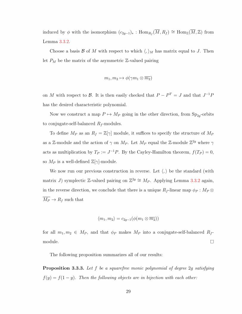
Choose a basis B of M with respect to which 〈, 〉M has matrix equal to J . Then
let PM be the matrix of the asymmetric Z-valued pairing
m1,m2 7→ φ(γm1 ⊗m2)
on M with respect to B. It is then easily checked that P − P T = J and that J−1P
has the desired characteristic polynomial.
Now we construct a map P 7→ MP going in the other direction, from Sp2g-orbits
to conjugate-self-balanced Rf -modules.
To define MP as an Rf = Z[γ] module, it suffices to specify the structure of MP
as a Z-module and the action of γ on MP . Let MP equal the Z-module Z2g where γ
acts as multiplication by TP := J−1P . By the Cayley-Hamilton theorem, f(TP ) = 0,
so MP is a well-defined Z[γ]-module.
We now run our previous construction in reverse. Let 〈, 〉 be the standard (with
matrix J) symplectic Z-valued pairing on Z2g ∼= MP . Applying Lemma 3.3.2 again,
in the reverse direction, we conclude that there is a unique Rf -linear map φP : MP ⊗
MP → Rf such that
〈m1,m2〉 = c2g−1(φ(m1 ⊗m2))
for all m1,m2 ∈ MP , and that φP makes MP into a conjugate-self-balanced Rf -
module.
The following proposition summarizes all of our results:
Proposition 3.3.3. Let f be a squarefree monic polynomial of degree 2g satisfying
f(y) = f(1− y). Then the following objects are in bijection with each other:
29

• Conjugate-self-balanced ideal classes of the ring Rf = Z[y]/f(y)
• Conjugate-self-balanced modules over Rf = Z[y]/f(y)
• Sp2g-equivalence classes of Seifert-parity 2g × 2g symmetric matrices Q such
that the characteristic polynomial of J−1Q is equal to 22gf((x− 1)/2)
• Sp2g-equivalence classes of asymmetric pairing matrices P with P − P T = J
and such that the characteristic polynomial of J−1P is equal to f(y)
• Simple Seifert hypersurfaces V such that, for one or any symplectic basis B of
Hq(V ), the matrix P of the asymmetric Seifert pairing p(γ, γ′) = lk(γ, (γ′)+)
with respect to B satisfies the property that the characteristic polynomial of
(J−1P ) is equal to f(y)
• Simple Seifert hypersurfaces V such that the Alexander polynomial ∆(t) of the
knot ∂V is equal to (1− t)2gf(1/(1− t)).
30

Chapter 4
Connections to the Alexander
module and related knot invariants
So far, we have only discussed invariants of Seifert hypersurfaces. In this section we
will discuss how they relate to known invariants of knots.
Let V be a Seifert hypersurface in S2q+1, and let P be a Seifert matrix for V with
respect to a symplectic basis of Hq(V ).
The matrix P is unique up to Sp2g-equivalence. Hence we can apply the invariants
constructed in the previous section. We define an invariant polynomial
fV (y) = det(yI − J−1P ). (4.1)
We also define an invariant conjugate-self-balanced module [MV , φV ] over the ring
RfV = Z[y]/fV (y). When the polynomial fV (y) is squarefree, we can also define the
corresponding conjugate-self-balanced ideal class [IV , αV ].
In this chapter, we will show:
• after change of variables, fV becomes an Alexander polynomial for the boundary
knot K = ∂V .
31

• after localization, the conjugate-self-balanced module MV becomes identified
with the Alexander module of K.
4.1 The Alexander polynomial
We now describe the relationship between the polynomial fV and the Alexander
polynomial of K coming from q-dimensional homology. As a result, we will see that
fV depends only on the boundary knot K = ∂V and on the genus g of V .
We first review the standard definition of the Alexander polynomial in terms of
the Alexander module.
Recall that we have defined (S2q+1 −K)cyc to be the unique infinite cyclic cover
of S2q+1 − K. Let t be the “positively oriented” generator of the group of deck
transformations of (S2q+1 − K)cyc (where this orientation is defined in terms of the
orientations on S2q+1 and on K). Then t has an induced action on all homology groups
of (S2q+1 −K)cyc. We can extend this action to give a Z[t, t−1]-module structure on
those homology groups. These modules are referred to as the Alexander modules of
K. In the setting of simple knots, the only nontrivial Alexander module is the one
coming from qth homology, which we will refer to as the Alexander module.
Definition. We define the Alexander module AlexK of K as the Z[t, t−1]-module
Hq((S2q+1 −K)cyc,Z).
We may define the Alexander polynomial for this Alexander module.
Definition. The Alexander polynomial ∆K is the generator of the first Fitting ideal
of the Z[t, t−1]-module AlexK , which is well-defined up to multiplication by units in
Z[t, t−1].
We have a choice about how to normalize it. The standard choice is the unique
normalization which makes ∆K(t) is a polynomial in t with nonzero constant term
satisfying ∆K(1) = 1, which is always possible.
32
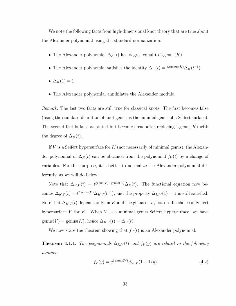
We note the following facts from high-dimensional knot theory that are true about
the Alexander polynomial using the standard normalization.
• The Alexander polynomial ∆K(t) has degree equal to 2 genus(K).
• The Alexander polynomial satisfies the identity ∆K(t) = t2 genus(K)∆K(t−1).
• ∆K(1) = 1.
• The Alexander polynomial annihilates the Alexander module.
Remark. The last two facts are still true for classical knots. The first becomes false
(using the standard definition of knot genus as the minimal genus of a Seifert surface).
The second fact is false as stated but becomes true after replacing 2 genus(K) with
the degree of ∆K(t).
If V is a Seifert hypersurface for K (not necessarily of minimal genus), the Alexan-
der polynomial of ∆K(t) can be obtained from the polynomial fV (t) by a change of
variables. For this purpose, it is better to normalize the Alexander polynomial dif-
ferently, as we will do below.
Note that ∆K,V (t) = tgenus(V )−genus(K)∆K(t). The functional equation now be-
comes ∆K,V (t) = t2 genus(V )∆K,V (t−1), and the property ∆K,V (1) = 1 is still satisfied.
Note that ∆K,V (t) depends only on K and the genus of V , not on the choice of Seifert
hypersurface V for K. When V is a minimal genus Seifert hypersurface, we have
genus(V ) = genus(K), hence ∆K,V (t) = ∆K(t).
We now state the theorem showing that fV (t) is an Alexander polynomial.
Theorem 4.1.1. The polynomials ∆K,V (t) and fV (y) are related in the following
manner:
fV (y) = y2 genus(V )∆K,V (1− 1/y) (4.2)
33

and
∆K,V (t) = (1− t)2 genus(V )fV (1/(1− t)). (4.3)
Proof. This follows from the standard formula ∆K,V (t) = det(Pt−P T ) and algebraic
manipulations.
4.2 Conjugate-self-balanced O∆-modules
We now wish to compare the Alexander module AlexK of a knot K with the invariant
conjugate-self-balanced module MV constructed in Section 3.3.
Again, let V be a simple Seifert hypersurface with boundary knot K. Let f(y) =
fV (y) be the invariant polynomial for V , and let ∆(t) = ∆K(t) be the Alexander
polynomial of K. For convenience we will restrict our attention to the case when the
matrix P is nonsingular, which is equivalent to the condition that genusK = genusV .
This implies that ∆K,V has nonzero constant term and is equal to ∆ = ∆K .
To do this, we must first change our point of view on the Alexander module. As
it stands, the Alexander module is a module over the ring Z[t, t−1], while MV is a
module over Rf = Z[y]/fV (y). However, the Alexander module is annihilated by
the Alexander polynomial ∆(t), and thus can also be viewed as a module over the
quotient ring, which we now give a name.
Definition. Let
O∆ = Z[t, t−1]/∆(t).
Let θ denote the image of t in O∆, so that O∆ = Z[θ, θ−1].
The ring O∆ has a natural involution interchanging θ with θ−1. We denote it by
x 7→ x.
34
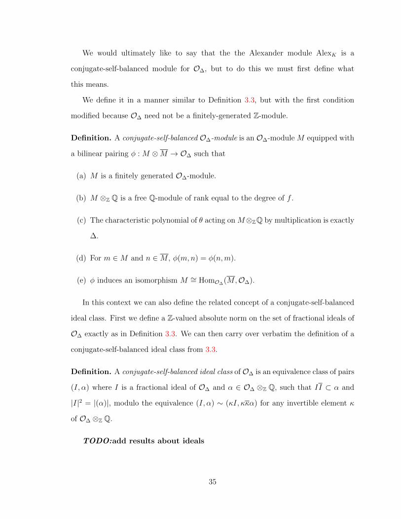
We would ultimately like to say that the the Alexander module AlexK is a
conjugate-self-balanced module for O∆, but to do this we must first define what
this means.
We define it in a manner similar to Definition 3.3, but with the first condition
modified because O∆ need not be a finitely-generated Z-module.
Definition. A conjugate-self-balanced O∆-module is an O∆-module M equipped with
a bilinear pairing φ : M ⊗M → O∆ such that
(a) M is a finitely generated O∆-module.
(b) M ⊗Z Q is a free Q-module of rank equal to the degree of f .
(c) The characteristic polynomial of θ acting on M⊗ZQ by multiplication is exactly
∆.
(d) For m ∈M and n ∈M , φ(m,n) = φ(n,m).
(e) φ induces an isomorphism M ∼= HomO∆(M,O∆).
In this context we can also define the related concept of a conjugate-self-balanced
ideal class. First we define a Z-valued absolute norm on the set of fractional ideals of
O∆ exactly as in Definition 3.3. We can then carry over verbatim the definition of a
conjugate-self-balanced ideal class from 3.3.
Definition. A conjugate-self-balanced ideal class of O∆ is an equivalence class of pairs
(I, α) where I is a fractional ideal of O∆ and α ∈ O∆ ⊗Z Q, such that II ⊂ α and
|I|2 = |(α)|, modulo the equivalence (I, α) ∼ (κI, κκα) for any invertible element κ
of O∆ ⊗Z Q.
TODO:add results about ideals
35
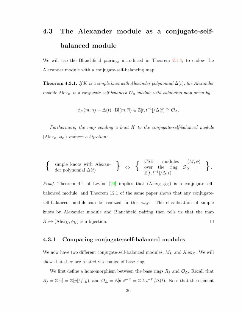
4.3 The Alexander module as a conjugate-self-
balanced module
We will use the Blanchfield pairing, introduced in Theorem 2.1.4, to endow the
Alexander module with a conjugate-self-balancing map.
Theorem 4.3.1. If K is a simple knot with Alexander polynomial ∆(t), the Alexander
module AlexK is a conjugate-self-balanced O∆-module with balancing map given by
φK(m,n) = ∆(t) · Bl(m,n) ∈ Z[t, t−1]/∆(t) ∼= O∆.
Furthermore, the map sending a knot K to the conjugate-self-balanced module
(AlexK , φK) induces a bijection:
{ simple knots with Alexan-der polynomial ∆(t)
} ⇔ { CSB modules (M,φ)over the ring O∆ =Z[t, t−1]/∆(t)
}.Proof. Theorem 4.4 of Levine [20] implies that (AlexK , φK) is a conjugate-self-
balanced module, and Theorem 12.1 of the same paper shows that any conjugate-
self-balanced module can be realized in this way. The classification of simple
knots by Alexander module and Blanchfield pairing then tells us that the map
K 7→ (AlexK , φK) is a bijection.
4.3.1 Comparing conjugate-self-balanced modules
We now have two different conjugate-self-balanced modules, MV and AlexK . We will
show that they are related via change of base ring.
We first define a homomorphism between the base rings Rf and O∆. Recall that
Rf = Z[γ] = Z[y]/f(y), and O∆ = Z[θ, θ−1] = Z[t, t−1]/∆(t). Note that the element
36

1− θ is a unit of O∆, because ∆(1) = 1, and that 11−θ is a root of the polynomial f
by (4.3). Hence the following homomorphism is well-defined:
Definition. Let ι : Rf → O∆ be the homomorphism from Rf to O∆ determined by
f(γ) = 11−θ .
Under our assumption that genusK = genusV , it is easily checked that ι is an
injection. Therefore ι identifies Rf with the subring of O∆ generated by 11−θ .
In the other direction, with the same assumption, one can also identify O∆ with
the localization Rf [(γγ)−1] = Rf [γ−1, (1 − γ)−1]. Here the element θ is identified
with 1 − γ−1, and θ−1 is identified with 1 − (1 − γ)−1. Under our assumption that
genus(K) = genus(V ), this induces an identification of the ring O∆⊗Q = Q[θ, θ−1] =
Q[θ] with Rf ⊗Q = Q[γ].
We now give the map from CSB(Rf ) to CSB(O∆).
Proposition 4.3.2. The map ι induces a map ι∗ from the set CSB(Rf ) of conjugate-
self-balanced Rf -modules to the set CSB(O∆) of conjugate-self-balanced O∆-modules,
given by
(M,V ) 7→ (M ⊗Rf O∆, φ⊗Rf O∆).
Proof. All conditions except the last are straightforward to check.
For the last one, we are given an isomorphism
M ∼= HomRf (M,Rf ).
Tensoring both sides with O∆ gives
M ⊗Rf O∆∼= HomRf (M,Rf )⊗Rf O∆.
37

Now, because O∆ is a flat Rf -module (it is a localization), it follows that (see exercise
1.2.8 in [22])
HomRf (M,Rf )⊗Rf O∆∼= HomO∆
(M ⊗Rf O∆,O∆).
Composing the two isomorphisms, we see that M ⊗Rf O∆ also satisfies the final
condition for a conjugate-self-balanced module.
We now show that ι∗ maps the conjugate-self-balanced module (MV , φV ) con-
structed from the Seifert pairing on V to the conjugate-self-balanced module
(AlexK , φK) coming from the Alexander module of K.
Theorem 4.3.3. We have
ι∗(MV , φV ) = (AlexK , φK).
Proof. Let P be a Seifert matrix for V . We will use explicit presentations, due to
Kearton, of the Alexander module and Blanchfield pairing of K in terms of P .
Kearton [17][§1] gave the following presentation of the Alexander module
O2g → O2g → AlexK → 0.
where the first map is multiplication by θP − P t. We will show that
ι∗(MV ) = MV ⊗Rf O∆
fits into the same exact sequence.
First, note that, because Rf is monogenic, there is a short exact sequence of
Rf -modules.
Rf ⊗Z Rf → Rf ⊗Z Rf → Rf → 0
38

where the first map is multiplication by 1⊗ γ − γ ⊗ 1 and the second map is induced
by the multiplication map Rf ×Rf → Rf .
By right exactness of the tensor product, we may tensor this sequence over Rf
with MV . This gives:
Rf ⊗Z MV → Rf ⊗Z MV →MV → 0.
Recall that we constructed MV by setting MArith = Z2g as a Z-module and having
γ act as left multiplication by J−1P . Using this identification of MV with Z2g, we
obtain a short exact sequence
R2gf → R2g
f →MV → 0,
where now the matrix of the first map is given by J−1P − γ = J−1 · (P − γJ), as
desired.
Now, tensoring over Rf with O∆, we get a short exact sequence
O2g∆ → O
2g∆ →MV → 0.
where the first map is left multiplication by J−1 · (P − ι(γ)J).
But
P − ι(γ)J = P − 1
1− θJ = (1− θ)−1((1− θ)P − (P − P T )) = −(1− θ)−1(θP − P T ).
Because J is invertible and −(1−θ)−1 is a unit of O∆, this means that there is another
short exact sequence
O2g∆ → O
2g∆ →MV → 0.
where the first map is left multiplication by θP − P t. This shows the first part.
39

To compare the conjugate-self-balancing maps, we use the presentation of the
Blanchfield pairing due to Kearton in [17, §8]. He shows that the Blanchfield pairing
Alex×Alex→ Q(t, t−1)/Z[t, t−1] is induced, in the presentation above, by the pairing
on O2g∆ with matrix (t− 1)(tP − P t)−1.
By the first half, we have AlexK ∼= MV ⊗Rf O∆, and so we can identify MV with
a submodule of O∆. Then it suffices to show that the restriction of φK to a bilinear
pairing MV ×MV → O∆ agrees with the pairing φV .
Recall from the proof of Theorem 3.3.1 that the pairing φV is uniquely character-
ized by the property that
〈m1,m2〉 = c2g−1(φV (m1 ⊗m2))
for all m1,m2 ∈MV .
It suffices to check that the restriction of φK has the same property.
Using Kearton’s presentation matrix for the Blanchfield pairing, it is a simple
computation to show that the matrix of the restriction of φK(m1 ⊗m2) to MV , with
respect to the standard basis, is given by (P −γ(J))ad (where ad refers to the adjoint
matrix from Cramer’s rule), and therefore the restricted pairing takes values in Rf .
We now apply c2g1 . The only terms with a γ2g−1 in the expansion of (P − γJ)ad
come from the (−γJ)ad = −γ2g−1Jad, and so c2g−1((P − γJ)ad) = −Jad = J .
Hence the pairing c2g−1(φV (m1 ⊗ m2)) also has matrix J with respect to the
standard basis of M ∼= Z2g, as desired.
40

4.3.2 Conjugate-self-balanced ideal classes of Dedekind rings
Before we move on to counting, we will note some ways in which the theory of
conjugate-self-balanced ideal classes is particularly nice when the base ring is a
Dedekind domain.
Recall that a Dedekind domain is a Noetherian integral domain of Krull dimension
1 which is integrally closed in its field of fractions. The rings Rf and O∆ are always
Noetherian and of Krull dimension 1, so they will be Dedekind domains precisely
when f (respectively ∆) is an irreducible polynomial and when Rf (respectively O∆)
is integrally closed.
Let A be a general Dedekind domain. Because every ideal of A is invertible,
the set of conjugate-self-balanced ideal classes of A forms a group with the natural
multiplication induced by multiplication of ideals: [I, α] · [I ′, α′] = [II ′, αα′]. This
group, which we will denote CSBA, has a natural homomorphism to the ideal class
group Cl(R) (see [18] for definition of the ideal class group of a Dedekind ring). This
homomorphism is given by forgetting α, and its image is exactly the kernel of the norm
map from Cl(R) to Cl(R1). On the other hand, the kernel of this homomorphism is the
image of the norm homomorphism on the unit groups R× → R×1 . We can summarize
this by saying that the group of conjugate-self-balanced ideal classes fits into a short
exact sequence
0→ R×1 /N(R×)→ CSBR → ker(N : Cl(R)→ Cl(R1))→ 0.
41
Chapter 5
Counting
5.1 Finiteness theorems for Seifert hypersurfaces
and simple knots
We would now like to put some notion of “size” on a knot in such a way that there are
only finitely many simple knots of bounded size. The following finiteness theorems
will be useful to us here.
Theorem 5.1.1 (Bayer and Michel,[1], Propositions 6 and 8).
• If ∆ ∈ Z[t] is a squarefree polynomial, there are only finitely many simple knots
K with ∆K = ∆.
• For any squarefree f ∈ Z[y], there are only finitely many simple Seifert hyper-
surfaces V such that fV = f .
Therefore, we can and will measure the size of K by the size of the Alexander
polynomial of K. For knots K of fixed genus g, we can measure this size by the size
of the coefficients of ∆K(t), or of fV (t) (where V is any genus g Seifert hypersurface).
There is still the question of how to “weight” the different coefficients with respect
to each other.
42

One way is to treat all coefficients equally; this leads to the standard definition of
the height of a polynomial.
Definition. The height ht(P ) of a polynomial P (x) = anxn+an−1x
n−1 + · · ·+a0x0 ∈
Z[x] is equal to
max0≤i≤n
|ai|.
One advantage of using height is that, for fixed g, the asymptotics for ht(fV (y))
are identical to those for ht(∆K,V (t)).
Note that ht(P ) < X if and only if all coefficients of P have absolute value at
most X.
For specific constrained families of polynomials, there may be other reasonable
ways to define size. For instance, for monic polynomials, we may defined a “weighted
height” function modeled after the definition in [4]
Definition. The weighted height htw(P ) of a monic polynomial
P (x) = xn + an−1xn−1 + · · ·+ a0x
0 ∈ Z[x]
is equal to
max0≤i≤n−1
|ai|n(n−1)/(n−i).
This definition is nice because it behaves nicely with respect to rescaling the
variable, that is, replacing P (x) with P (ax). However, such transformations do not
have an obvious interpretation in knot theory.
Since there are only finitely many integer polynomials with bounded height, we
obtain the following finiteness statement as a corollary of Theorem 5.1.1:
Corollary 5.1.2. • For any q ≥ 3 and g ≥ 0, and for any X, there are only
finitely many equivalence classes of simple Seifert hypersurfaces V in S2q+1 of
genus g such that the Alexander polynomial ∆K(t) is squarefree of height ≤ X.
43
• For any q ≥ 3 and g ≥ 0, and for any X, there are only finitely many simple
2q− 1-knots of genus g such that the Alexander polynomial ∆K(t) is squarefree
of height ≤ X.
5.2 Strategies
We will now use the algebraic machinery developed in the previous chapter to tackle
the following asymptotic counting question:
Question. How many simple 2q− 1-knots of genus g have squarefree Alexander poly-
nomial of height ≤ X?
We will also ask the analogous question for Seifert hypersurfaces:
Question. How many simple Seifert hypersurfaces of genus g in S2q+1 have squarefree
Alexander polynomial of height ≤ X?
Both of these (originally topological) questions can be converted into purely arith-
metic questions by means of Theorem 2.2.1. We now discuss these arithmetic ques-
tions.
We have seen that Seifert hypersurfaces are in bijection with the Sp2g orbits on
Seifert-parity symmetric matrices. These orbits can be counted using general methods
from the geometry of numbers for counting orbits of an algebraic group over Z acting
on a lattice in a vector space.
The most naıve of these is the following: find a fundamental domain R for the
action of Sp2g(Z) on Sym2(R2g), and let RX be the subregion of R consting of points
with height ≤ X. Then the orbits with Alexander polynomial of height ≤ X are in
bijection with lattice points in RX . We can get an approximate count of the latter
using the volume of RX .
This does not quite work as stated, because Sp2g(Z) does not act properly discon-
tinuously on all of Sym2(R2g). First, we need to omit the points where the Alexander
44

polynomial has repeated roots. This splits Sym2(R2g) into several connected com-
ponents. On some of these components, Sp2g(Z) does act properly discontinuously
and we can count orbits by counting lattice points in a fundamental domain. On the
others, there is no fundamental domain, and the counting problem is substantially
harder.
For example, in the case of genus 1, there are three connected components. The
ones coming from definite quadratic forms have fundamental domains, and their
counting question is very well-understood. The indefinite component is less well
understood, though heuristics suggest it contains a small number of orbits compared
to the others.
There are two difficulties with this approach. The first is that error terms become
more complicated to estimate as g gets large. A more specific issue is that the region
R is unbounded, with a cusp going off to infinity. In order to get a finite error term,
one must “chop off” the region at some point along the cusp, and deal with the cusp
separately.
In the case g = 1, the region R is 3-dimensional, and it is possible to do this
estimation explicitly. This was done, in the equivalent context of positive definite
binary quadratic forms, by a number of people, including Mertens [23]. We will use
these same methods to prove Theorem 5.3.2, which counts positive definite binary
quadratic forms with a congruence condition on the discriminant, which is an essential
ingredient to our sieving argument.
For larger g, this approach becomes more complicated. [5, 6, 4, 31] have recently
developed more streamlined methods for asymptotic orbit-counting. They count or-
bits by averaging over a continuously varying family of fundamental domains. The
author is currently working on applying these methods to count genus g Seifert hy-
persurfaces for g ≥ 1.
45
5.3 Counting genus 1 Seifert hypersurfaces
5.3.1 2×2 Seifert-parity symmetric matrices, binary quadratic
forms, and ideals in quadratic rings
In the simplest example where V has genus 1, the polynomial fV will be of the form
x2 − x + m, for an arbitrary integer m. If m 6= 0, the boundary knot K will also
have genus 1, and the Alexander polynomial ∆K of the boundary knot K will be
mt2 + (1− 2m)t+m. We henceforward assume that m is nonzero.
The corresponding ring Rf = Z[y]/(y2−y+m) = Z[1+√
1−4m2
] is a quadratic ring of
Z with discriminant 1− 4m. If 1− 4m is not square, Rf is an order in the quadratic
field Q[√
1− 4m], and if 1 − 4m is squarefree, Rf is the entire ring of integers of
Q[√
1− 4m].
The ring O∆ also has a nice form: it is equal to Z[ 1m,√
1− 4m], and can be viewed
as a quadratic extension of the ring Z[ 1m
] with discriminant 1− 4m.
In this setting, all the “size functions” we have considered are the same up to
linear change of variables. The height of fv is |m| and the height of ∆K is |2m− 1|.
Now we consider conjugate-self-balanced ideal classes in the rings Rf and O∆.
We now show that any ideal class of these rings can be equipped with a (not
necessarily unique) balancing map.
Lemma 5.3.1. (i) If I is an ideal of Rf , and a = |I| = [Rf : I] is the absolute
norm of the ideal I, then [I, a] and [I,−a] are (possibly equal) conjugate-self-
balanced ideal classes of Rf .
(ii) The same is true of O∆.
(iii) The set of conjugate-self-balanced ideal classes of Rf = Z[1+√
1−4m2
] can be iden-
tified with the set of oriented ideal classes of Rf , as defined in [2]. These are
the ideal classes I of Rf equipped with an isomorphism of Z-modules∧2 I → Z.
46

(iv) The number of simple Seifert hypersurfaces of genus 1 with Alexander polynomial
mt2 + (1− 2m)t+m is equal to the narrow class number of Rf .
Proof. Part (i) amounts to saying that |(a)| = a2 and II ⊂ (a). These are both
standard facts from the theory of imaginary quadratic orders. Part (ii) is analogous.
For (iii), recall the map c1 = c2g−1 from Definition 3.3. We have explicitly
c1(x+ yγ) = y.
By the proof of Theorem 3.3.1, the map I × I → Z given by i1, i2 7→ c1(i1i2/a) is
a perfect skew-symmetric pairing, and so induces an orientation on I. The other
direction of the proof of Theorem 3.3.1 shows that any orientation on I arises in this
way.
Finally, (iv) follows from the definition of the narrow class number as the number
of oriented ideal classes of I.
Fortunately for us, the asymptotics for the average behavior of the narrow class
number of quadratic rings are well-understood, as we shall see next.
5.3.2 Counting Seifert forms of negative discriminant
Because the Seifert form of a Seifert hypersurface uniquely determines the isotopy
type of its boundary knot, one can obtain an upper bound for the number of genus
1 knots with Alexander polynomial mt2 + (1− 2m)t+m by counting the number of
SL2(Z)-equivalence classes of Seifert-parity binary quadratic forms with that Alexan-
der polynomial. It is easier to do this counting if we average over all m within a
certain range.
It turns out that one gets two different types of behavior depending upon whether
the form is definite (signature 2 or −2), or indefinite (signature 0).
47
The problem of counting binary quadratic forms of bounded discriminant is a
classical one in number theory and the additional condition of Seifert parity is very
minor: in fact, it is just a parity condition on the discriminant. In the definite case,
one can obtain an asymptotic result via the geometry of numbers as done in [23].
The indefinite case is much harder; the same methods used in the definite case obtain
an upper bound of the same size, but standard heuristics suggest that the answer is
much lower. Our geometry of numbers argument here will be essentially the same as
that used in [23].
Ultimately we will prove a more general result that will be useful in the next
section:
Theorem 5.3.2. Let X be a real number, and let s be a positive integer with s ≤ X.
The number of Seifert-parity definite (m > 0) binary quadratic forms with Alexander
polynomial mt2 + (1− 2t)x+m where |m| < X and s | m is asymptotically equal to
c1ρ(s)X3/2 +O(ρ(s)sX max(s, logX)). (5.1)
Here ρ(s) =∏
p|sp+1p2 . The value of the constant c1 can be made explicit, as can the
constant implicit in the big-O notation for the error term, but we will not compute
them here.
The number of Seifert-parity indefinite (m ≤ 0) binary quadratic forms with
Alexander polynomial mt2 + (1 − 2m)t + m where |m| < X is bounded by a con-
stant times X3/2.
Remark. The bound for the indefinite case is extremely weak. The heuristics of Hooley
[15] suggest that the actual asymptotic should be X(logX)2.
It is also possible to get an upper bound of the same form as (5.1) for the number
of indefinite forms with s | m, but this is not useful to us.
48
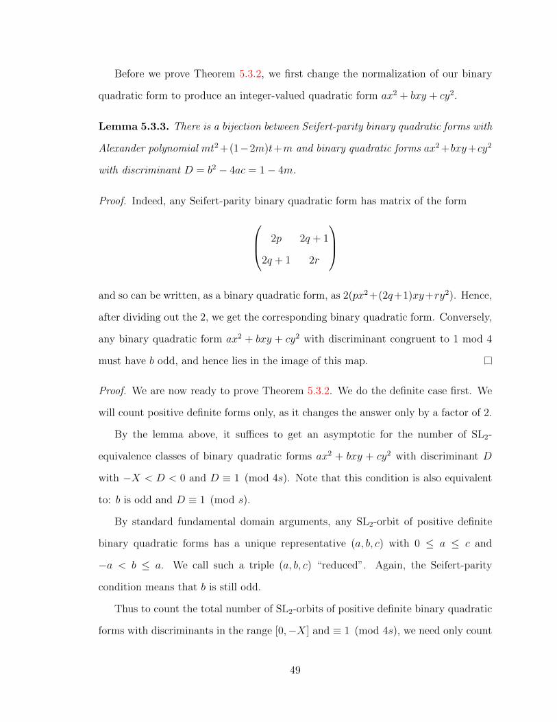
Before we prove Theorem 5.3.2, we first change the normalization of our binary
quadratic form to produce an integer-valued quadratic form ax2 + bxy + cy2.
Lemma 5.3.3. There is a bijection between Seifert-parity binary quadratic forms with
Alexander polynomial mt2 +(1−2m)t+m and binary quadratic forms ax2 +bxy+cy2
with discriminant D = b2 − 4ac = 1− 4m.
Proof. Indeed, any Seifert-parity binary quadratic form has matrix of the form
2p 2q + 1
2q + 1 2r
and so can be written, as a binary quadratic form, as 2(px2 +(2q+1)xy+ry2). Hence,
after dividing out the 2, we get the corresponding binary quadratic form. Conversely,
any binary quadratic form ax2 + bxy + cy2 with discriminant congruent to 1 mod 4
must have b odd, and hence lies in the image of this map.
Proof. We are now ready to prove Theorem 5.3.2. We do the definite case first. We
will count positive definite forms only, as it changes the answer only by a factor of 2.
By the lemma above, it suffices to get an asymptotic for the number of SL2-
equivalence classes of binary quadratic forms ax2 + bxy + cy2 with discriminant D
with −X < D < 0 and D ≡ 1 (mod 4s). Note that this condition is also equivalent
to: b is odd and D ≡ 1 (mod s).
By standard fundamental domain arguments, any SL2-orbit of positive definite
binary quadratic forms has a unique representative (a, b, c) with 0 ≤ a ≤ c and
−a < b ≤ a. We call such a triple (a, b, c) “reduced”. Again, the Seifert-parity
condition means that b is still odd.
Thus to count the total number of SL2-orbits of positive definite binary quadratic
forms with discriminants in the range [0,−X] and ≡ 1 (mod 4s), we need only count
49

the number of lattice points (a, b, c) in the region
RX = {(x, y, z) ∈ R3 | 0 ≤ x ≤ z,−x < y ≤ x, 0 < y2 − 4xz ≤ X}
such that b2 − 4ac ≡ 1 (mod 4s).
Our strategy will be to use Davenport’s theorem on counting integer lattice points
inside regions.
Theorem 5.3.4 (Davenport [9]). Let R be a bounded semi-algebraic region in Rn,
defined by k polynomial inequalities of degree at most `. Then the number of points
(a, b, c) ∈ Zn ∩R can be asymptotically expressed as
vol(R) + ε(R)
with the error term ε(R) bounded in size by ε(R) < κmax(R, 1) where R runs
over all projections of R onto subspaces of Rn spanned by coordinate axes, and
κ = κ(n,m, k, `) is some explicit constant depending only on n,m, k, and `.
We will be unable to apply Davenport’s theorem to RX , because some of its
shadows have infinite volume. Therefore we will use a truncated region, RX,t =
{(x, y, z) ∈ R | z < t}.
We now state some facts about the size of the various projections onto coordinate
axes and planes. Let Px, Py, Pz denote the projection maps onto the x, y, z axes
respectively, and likewise define Px,y, Px,z, Py,z as the projections onto the coordinate
planes.
Lemma 5.3.5. We have the following bounds:
vol(RX,t) = c0X3/2 +O(t−3X3), (5.2)
50

area(Px,y(RX,t)) = O(X) (5.3)
area(Px,z(RX,t)) = O(X log(tX−1/2))) (5.4)
area(Py,z(RX,t)) = O(X log(tX−1/2)), (5.5)
and
length(Px(RX,t)) = O(X1/2) (5.6)
length(Py(RX,t)) = O(X1/2) (5.7)
length(Pz(RX,t)) = t. (5.8)
Proof. This is a calculation.
We first prove (5.1) for the case when s = 1. Note that if (a, b, c) is a lattice point
in R, then c can be at most 14(X + 1) ≤ X. Therefore all lattice points in RX also
belong to the truncated region RX,X , and we may count the latter instead. To do
this, we estimate the number of lattice points in the region RX,t for general t and
then set t = X.
Note that we are not counting all lattice points, only the ones with b odd. How-
ever, we can apply an affine transformation to the second coordinate, to convert our
question into one about counting lattice points.
We then apply Davenport’s theorem, and set t = X
#(RX,t ∩ Z3) = c1X3/2 +O(max(X log(tX−1/2), t)) = c1X
3/2 +O(X logX). (5.9)
Now we do the same analysis, but with s a general positive integer. The following
lemma will allow us to replicate the argument above.
51
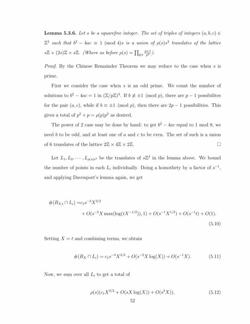
Lemma 5.3.6. Let s be a squarefree integer. The set of triples of integers (a, b, c) ∈
Z3 such that b2 − 4ac ≡ 1 (mod 4)s is a union of ρ(s)s3 translates of the lattice
sZ× (2s)Z× sZ. (Where as before ρ(s) =∏
p|sp+1p2 ).
Proof. By the Chinese Remainder Theorem we may reduce to the case when s is
prime.
First we consider the case when s is an odd prime. We count the number of
solutions to b2 − 4ac = 1 in (Z/pZ)3. If b 6≡ ±1 (mod p), there are p− 1 possibilites
for the pair (a, c), while if b ≡ ±1 (mod p), then there are 2p− 1 possibilities. This
gives a total of p2 + p = ρ(p)p3 as desired.
The power of 2 case may be done by hand: to get b2 − 4ac equal to 1 mod 8, we
need b to be odd, and at least one of a and c to be even. The set of such is a union
of 6 translates of the lattice 2Z× 4Z× 2Z.
Let L1, L2, · · · , Lρ(s)s3 be the translates of sZ3 in the lemma above. We bound
the number of points in each Li individually. Doing a homothety by a factor of s−1,
and applying Davenport’s lemma again, we get
#(RX,t ∩ Li) =c1s−3X3/2
+O(s−2X max(log(tX−1/2)), 1) +O(s−1X1/2) +O(s−1t) +O(1).
(5.10)
Setting X = t and combining terms, we obtain
#(RX ∩ Li) = c1s−3X3/2 +O(s−2X log(X)) +O(s−1X). (5.11)
Now, we sum over all Li to get a total of
ρ(s)(c1X3/2 +O(sX log(X)) +O(s2X)), (5.12)
52

as desired.
The upper bound for indefinite forms can be proved in a similar manner, by
noting that any indefinite form is SL2-equvalent to at least one such with (a, b, c)
with 0 ≤ |a| ≤ |c| and −|a| < b ≤ |a|.
Alternatively, it can be proved by showing a result using regulators.
5.3.3 Counting Seifert forms of positive discriminant
We now consider counting the Seifert forms with positive description, namely, the
indefinite quadratic forms. The crude bound given above is far from tight. We
expect the following heuristic:
Heuristic 1. The total number of indefinite Seifert-parity quadratic forms whose
Alexander polynomial is mt2 + (1− 2m)t+m with m ∈ [1, X] is asymptotic to
c3X(logX)2.
The justification for this is that, as we have seen, indefinite Seifert-parity quadratic
forms are the same as indefinite binary quadratic forms with odd discrimiant. Hooley
[15] gives an asymptotic proportional to X(logX)2 for all indefinite binary quadratic
forms, and
Comparing with the bound for definite quadratic forms, we see that, according to
the heuristic, most genus 1 Seifert pairings have symmetric part which is definite.
5.4 Counting genus 1 simple knots
5.4.1 The map ι∗
We now move to the question of conuning equivalence classes of genus 1 simple knots,
which we have put in bijection with conjugate-self-balanced ideal classes of O∆.
53

It is harder to count conjugate-self-balanced ideal classes of O∆, because they are
not in one-to-one correspondence with Z-orbits of an arithmetic group. However, we
do have the surjection
ι∗ : CSB(Rf ) � CSB(O∆).
This map is a homomorphism of monoids, and when 1− 4m is squarefree it is also a
group homomorphism. We wish to know what we can say about its fibers.
Because we are working with conjugate-self-balanced ideal classes of both Rf and
O∆, we will use subscripts to clarify: we will write [I, α]Rf to specify that we mean
an element of CSB(Rf ).
In that case, we have the following criterion:
Lemma 5.4.1. Suppose that I and J are ideals of Rf such that IO∆ = JO∆. Then
I = aJ for some fractional ideal a of Rf of the form
a =∏p|m
pep (5.13)
where the product is over all ideals p of Rf dividing m.
Proof. The condition I = aJ holds if and only if it holds locally at all primes of Rf ,
that is, if and only if I(Rf )q = aJ(Rf )q for all primes q of Rf .
First consider the case when q divides m. Then q is invertible and the localization
(Rf )q is a DVR. So we can pick eq to satisfy the condition at q.
For each q that does not divide m, the ring O∆ = Rf [1/m] is contained in (Rf )q,
and so the condition I(Rf )q = J(Rf )q is automatically satisfied.
Because O∆ = Rf [1/m] is obtained from Rf by inverting the element m, it will
be useful for us to know the factorization of the ideal mRf in Rf . Fortunately for us,
mRf has an explicit factorization as a product of distinct prime ideals of Rf , given
54

by
mRf =∏p|m
(p, γ) · (p, 1− γ). (5.14)
where p ranges over all prime factors of m in Z.
The following observation is easily checked, and will be useful later on: if p is a
prime factor of mRf , then pp is a principal ideal generated by some prime factor (p)
of m. As a consequence, p is an invertible ideal of Rf .
We may then refer to the primes appearing in (5.14) as “the prime factors of
mRf”.
We now use these prime factors to define a special subgroup of K of CSB(Rf )
which we will see we can view as the “kernel” of the monoid homomorphism ι.
Definition. Let K be the subgroup of the monoid CSB(Rf ) generated by
[p(p)−1, 1]Rf ,
where p ranges over the set of prime factors of mRf .
Because pp is a principal ideal for any prime factor p of Rf , this definition can also
be restated as follows: K is the subgroup of CSB(Rf ) generated by [p2, |p|2] = [p, |p|]2
where p ranges over the prime factors of mRf .
Theorem 5.4.2. A conjugate-self-balanced ideal class [I, α]Rf ∈ CSB(Rf ) maps to
the identity under ι∗ if and only if [I, α]Rf ∈ K.
More generally, the ideals [I, α]Rf , [J, β]Rf ∈ CSB(Rf ) map to the same element
of CSB(O∆) if and only if [I, α]Rf = k[J, β]Rf for some k ∈ K.
Proof. We will prove the second part, which is a strictly stronger statement (because
CSB(Rf ) is a monoid and not a group).
For the “only if” direction, it suffices to show that generators of K are sent to the
identity by ι∗. This is easily checked.
55

For the other direction, suppose that
ι([I, α]Rf ) = ι([J, β]Rf ).
It follows from the definitions that IO∆ = cJO∆ and α = ccβ for some c ∈ FracO∆ =
FracRf . Let I ′ = c−1I, so that
[I, α]Rf = [c−1I, cc−1α] = [I ′, β]Rf .
Hence I ′O∆ = JO∆, and Lemma 5.4.1 applies, so we can write I ′ = aJ , where a
is a product of (possibly negative) powers of primes dividing m.
By comparing I ′I ′ with JJ , and localizing at each prime dividing m, we can show
that a is a product of ideals of the form p−1p, where p | m, as desired.
This theorem has the following useful consequences. Recall that the 2-rank of an
abelian group G (with the action written multiplicatively) is the rank of the F2-vector
space G/G2.
Corollary 5.4.3. The 2-rank of NCl(O∆) is the same as the 2-rank of the narrow
class group NCl(Rf ).
Remark. This 2-rank can be computed explicitly using genus theory.
Corollary 5.4.4. Suppose that m > 0. Then the map ι∗ : NCl(Rf )→ NCl(O∆) is a
bijection if and only if m is prime.
Proof. Proof of ⇒: Suppose that m is not prime, and let p be a prime factor of m.
Then the ideal (p, γ) is a prime factor of m with norm p, but cannot be principal
because Rf = Z[1−4m2
] does not contain any elements of norm strictly less than m.
Proof of ⇐: In this case m = p is prime, and γ(1 − γ) = p. Hence pRf factors
as the product of the two principal ideals (p, γ) = (γ) and (p, 1− γ) = (1− γ).
56

In this case, we will wish to divide up into cases, depending upon whether or not
m is prime. As seen above, if m is a prime, the map ι∗ is a bijection, whereas in the
case where m is composite, it cannot be one-to-one. Therefore we will get a larger
answer in the case when m is prime. We quantify this below.
We can use the bounds in Theorem 5.3.2, to show
Theorem 5.4.5. The total number of distinct Alexander modules (with pairing) hav-
ing Alexander polynomial equal to pt2 + (1 − 2p)t + p for p running over all primes
in the range [1, X] is (unconditionally) bounded above by O(X3/2/ logX).
Proof. We will prove this by proving the following statement, which will imply the
desired result. For any real number z, let P (z) =∏
p prime <z p. Let α be a real
constant, whose value will be chosen later, but will satisfy α < 1.
Then it will suffice to show:
∑X≤m≤2X
(m,P (Xα))=1
#((a, b, c) ∈ Z3 : b2 − 4ac = 1− 4m) = O(X3/2/ logX). (5.15)
5.4.2 A sieving argument
We follow the approach of Rosser’s sieve [16], modifying the terminology to suit our
approach. We name the quantity that we wish to bound:
S(X, z) :=∑
X≤m≤2X(m,P (z))=1
#{(a, b, c) ∈ Z3 : b2 − 4ac = 1− 4m}
for z = Xα.
To apply the sieve, we need estimates on the following quantities for all squarefree
d:
Sd(X, z) :=∑
m∈[X,2X]d|m
#{(a, b, c) ∈ Z3 : b2 − 4ac = 1− 4m}. (5.16)
57
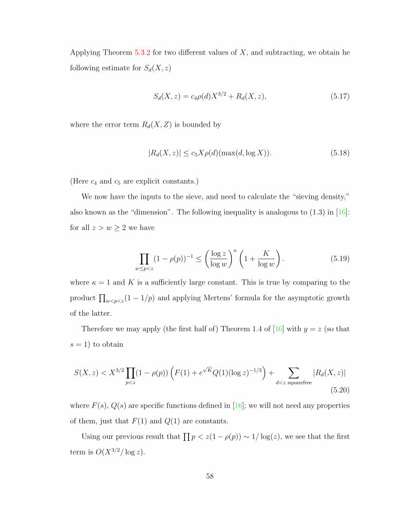
Applying Theorem 5.3.2 for two different values of X, and subtracting, we obtain he
following estimate for Sd(X, z)
Sd(X, z) = c4ρ(d)X3/2 +Rd(X, z), (5.17)
where the error term Rd(X,Z) is bounded by
|Rd(X, z)| ≤ c5Xρ(d)(max(d, logX)). (5.18)
(Here c4 and c5 are explicit constants.)
We now have the inputs to the sieve, and need to calculate the “sieving density,”
also known as the “dimension”. The following inequality is analogous to (1.3) in [16]:
for all z > w ≥ 2 we have
∏w≤p<z
(1− ρ(p))−1 ≤(
log z
logw
)κ(1 +
K
logw
). (5.19)
where κ = 1 and K is a sufficiently large constant. This is true by comparing to the
product∏
w<p<z(1− 1/p) and applying Mertens’ formula for the asymptotic growth
of the latter.
Therefore we may apply (the first half of) Theorem 1.4 of [16] with y = z (so that
s = 1) to obtain
S(X, z) < X3/2∏p<z
(1− ρ(p))(F (1) + e
√KQ(1)(log z)−1/3
)+
∑d<z squarefree
|Rd(X, z)|
(5.20)
where F (s), Q(s) are specific functions defined in [16]; we will not need any properties
of them, just that F (1) and Q(1) are constants.
Using our previous result that∏p < z(1− ρ(p)) ∼ 1/ log(z), we see that the first
term is O(X3/2/ log z).
58

Applying (5.18) to the second term gives
∑d<z squarefree
|Rd(X, z)| ≤ c5X∑
d<z squarefree
ρ(d)d(max(d, logX)). (5.21)
We estimate ρ(d). Since d is squarefree, we can write d as a product of distinct
primes: d =∏nd
i=1 pi. Then
ρ(d) =
nd∏i=1
pi + 1
p2i
=1
d
nd∏i=1
(1 +
1
pi
)=
1
d
∑d′|d
1
d′
≤ 1
d
∑1≤d′≤z
1
d′
≤ log z + 1
d.
(5.22)
Plugging (5.22) into the sum in (5.21), we obtain
∑d<z squarefree
|Rd(X, z)| ≤ c5X(log z + 1)∑d<z
max(d, log x)
≤ c5(log z + 1)∑d<z
(d+ logX)
≤ c5X(log z + 1)(z2 + z logX)
≤ c5X(α logX + 1)(X2α +Xα logX).
(5.23)
In the last line we have set z = Xα.
For fixed α and X varying, we get the following asymptotics for our remainder
term
∑d<z squarefree
|Rd(X, z)| = O(X1+2α logX). (5.24)
59

This will be o(X3/2/ logX) for any α < 1, and so our error term is bounded.
5.4.3 Heuristics
Heuristically, we expect that this theorem is sharp. That is, we expect
Heuristic 2. The total number of distinct Alexander modules (with pairing) having
Alexander polynomial equal to pt2 + (1− 2p)t+ p for p running over all primes in the
range [1, X] is asymptotic to O(X3/2/ logX).
The error bound in Theorem 5.3.2 is too large to be used in the sieve to obtain a
lower bound. Although one can get better estimates by using the geometry of numbers
more carefully, this technique does not appear to give a sufficient improvement.
For all other discriminants, we expect there to be substantially fewer Alexander
modules.
Heuristic 3. The total number of distinct Alexander modules (with pairing) having
Alexander polynomial equal to mt2 + (1 − 2m)t + m for m running over all integers
in the range [−X,X] that are not positive primes is (heuristically) bounded above by
O(X(logX)2).
Combining the two heuristics above suggests the following, weaker, heuristic
Heuristic 4. Most Alexander modules (with pairing) have Alexander polynomial of
the form pt2 + (1 − 2p)t + p for p > 0 prime. Equivalently, most simple knots have
Alexander polynomal of the same form.
60
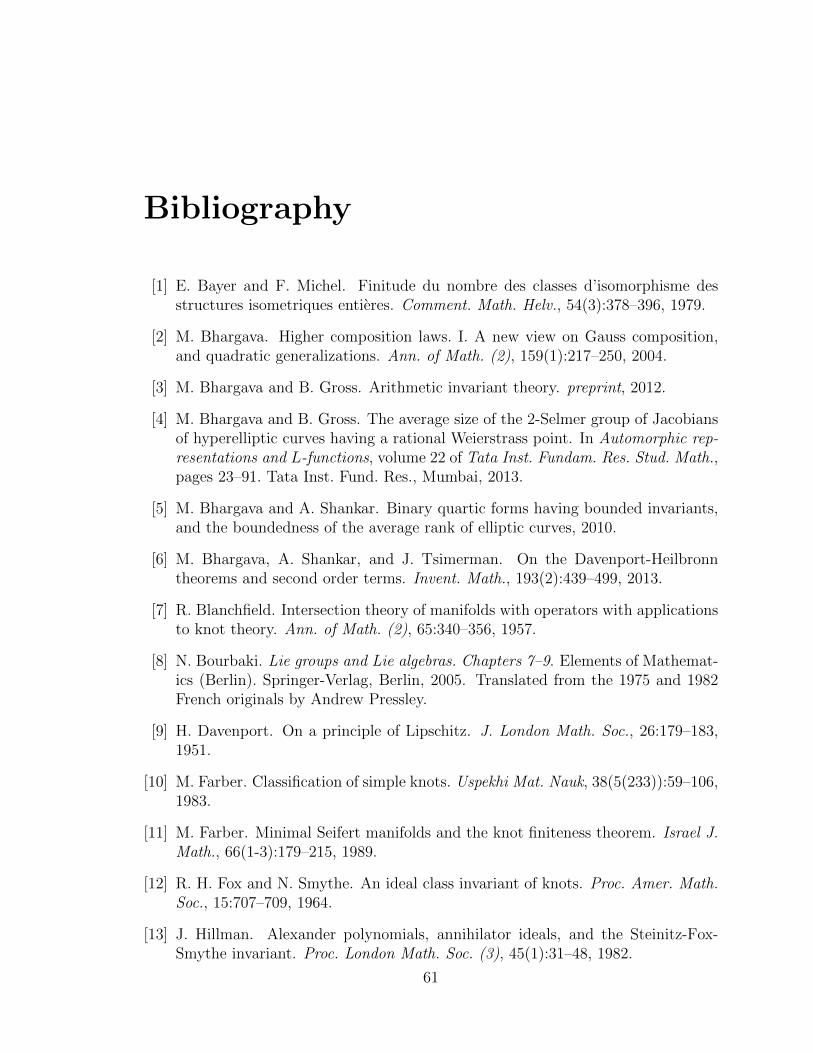
Bibliography
[1] E. Bayer and F. Michel. Finitude du nombre des classes d’isomorphisme desstructures isometriques entieres. Comment. Math. Helv., 54(3):378–396, 1979.
[2] M. Bhargava. Higher composition laws. I. A new view on Gauss composition,and quadratic generalizations. Ann. of Math. (2), 159(1):217–250, 2004.
[3] M. Bhargava and B. Gross. Arithmetic invariant theory. preprint, 2012.
[4] M. Bhargava and B. Gross. The average size of the 2-Selmer group of Jacobiansof hyperelliptic curves having a rational Weierstrass point. In Automorphic rep-resentations and L-functions, volume 22 of Tata Inst. Fundam. Res. Stud. Math.,pages 23–91. Tata Inst. Fund. Res., Mumbai, 2013.
[5] M. Bhargava and A. Shankar. Binary quartic forms having bounded invariants,and the boundedness of the average rank of elliptic curves, 2010.
[6] M. Bhargava, A. Shankar, and J. Tsimerman. On the Davenport-Heilbronntheorems and second order terms. Invent. Math., 193(2):439–499, 2013.
[7] R. Blanchfield. Intersection theory of manifolds with operators with applicationsto knot theory. Ann. of Math. (2), 65:340–356, 1957.
[8] N. Bourbaki. Lie groups and Lie algebras. Chapters 7–9. Elements of Mathemat-ics (Berlin). Springer-Verlag, Berlin, 2005. Translated from the 1975 and 1982French originals by Andrew Pressley.
[9] H. Davenport. On a principle of Lipschitz. J. London Math. Soc., 26:179–183,1951.
[10] M. Farber. Classification of simple knots. Uspekhi Mat. Nauk, 38(5(233)):59–106,1983.
[11] M. Farber. Minimal Seifert manifolds and the knot finiteness theorem. Israel J.Math., 66(1-3):179–215, 1989.
[12] R. H. Fox and N. Smythe. An ideal class invariant of knots. Proc. Amer. Math.Soc., 15:707–709, 1964.
[13] J. Hillman. Alexander polynomials, annihilator ideals, and the Steinitz-Fox-Smythe invariant. Proc. London Math. Soc. (3), 45(1):31–48, 1982.
61
[14] J. Hillman. Algebraic invariants of links, volume 32 of Series on Knots andEverything. World Scientific Publishing Co. Inc., River Edge, NJ, 2002.
[15] C. Hooley. On the Pellian equation and the class number of indefinite binaryquadratic forms. J. Reine Angew. Math., 353:98–131, 1984.
[16] H. Iwaniec. Rosser’s sieve. Acta Arith., 36(2):171–202, 1980.
[17] C. Kearton. Blanchfield duality and simple knots. Trans. Amer. Math. Soc.,202:141–160, 1975.
[18] S. Lang. Algebraic number theory. Addison-Wesley Publishing Co., Inc., Reading,Mass.-London-Don Mills, Ont., 1970.
[19] J. Levine. An algebraic classification of some knots of codimension two. Com-ment. Math. Helv., 45:185–198, 1970.
[20] J. Levine. Knot modules. I. Trans. Amer. Math. Soc., 229:1–50, 1977.
[21] J. Levine. Algebraic structure of knot modules, volume 772 of Lecture Notes inMathematics. Springer, Berlin, 1980.
[22] Q. Liu. Algebraic geometry and arithmetic curves, volume 6 of Oxford GraduateTexts in Mathematics. Oxford University Press, Oxford, 2002. Translated fromthe French by Reinie Erne, Oxford Science Publications.
[23] F. Mertens. Ueber einige asymptotische gesetze der zahlentheorie. Journal fr diereine und angewandte Mathematik, 77:289–338, 1874.
[24] J. Milnor. Singular points of complex hypersurfaces. Annals of MathematicsStudies, No. 61. Princeton University Press, Princeton, N.J., 1968.
[25] J. Milnor. On isometries of inner product spaces. Invent. Math., 8:83–97, 1969.
[26] J. Milnor and D. Husemoller. Symmetric bilinear forms. Springer-Verlag, NewYork-Heidelberg, 1973. Ergebnisse der Mathematik und ihrer Grenzgebiete,Band 73.
[27] J.-P. Serre. Galois cohomology. Springer Monographs in Mathematics. Springer-Verlag, Berlin, english edition, 2002. Translated from the French by Patrick Ionand revised by the author.
[28] J. Thorne. Vinberg’s representations and arithmetic invariant theory. AlgebraNumber Theory, 7(9):2331–2368, 2013.
[29] H. Trotter. On S-equivalence of Seifert matrices. Invent. Math., 20:173–207,1973.
[30] H. Trotter. Knot modules and Seifert matrices. In Knot theory (Proc. Sem.,Plans-sur-Bex, 1977), volume 685 of Lecture Notes in Math., pages 291–299.Springer, Berlin, 1978.
62
[31] K. Wilson. Three perspectives on n points in Pn−2. Princeton PhD Thesis, 2013.
[32] M. Wood. Parametrization of ideal classes in rings associated to binary forms.J. Reine Angew. Math., to appear.
63