
Countervailing power and input pricing: When is a waterbed ... · 1 DEPARTMENT OF ECONOMICS ISSN...
23
1 DEPARTMENT OF ECONOMICS ISSN 1441-5429 DISCUSSION PAPER 27/12 Countervailing power and input pricing: When is a waterbed effect likely? Stephen P. King 1 Abstract A downstream firm with countervailing power can extract a reduced price from an input supplier. A waterbed effect occurs if this price reduction leads the input supplier to raise the price that it charges another downstream firm. Policy makers have been concerned that this waterbed effect could undermine downstream competition, and it was considered in detail in the 2008 UK grocery inquiry. This paper presents a simple but parsimonious model to investigate if and when a waterbed effect may arise. It shows that the effect may arise through optimal pricing behaviour, but that this critically depends on the nature of upstream technology, downstream competition and consumer demand. In particular, downstream competition tends to work against a waterbed effect, but convex upstream costs support the effect. The analysis is complementary to recent academic work on the waterbed effect that focuses on bargaining constraints. 1 Department of Economics, Monash University, Caulfield East, Victoria, Australia; E-mail: [email protected] I would like to thank Y.K.Ng for comments on an earlier draft of this paper. © 2012 Stephen P. King All rights reserved. No part of this paper may be reproduced in any form, or stored in a retrieval system, without the prior written permission of the author.
Transcript of Countervailing power and input pricing: When is a waterbed ... · 1 DEPARTMENT OF ECONOMICS ISSN...
1
DEPARTMENT OF ECONOMICS
ISSN 1441-5429
DISCUSSION PAPER 27/12
Countervailing power and input pricing: When
is a waterbed effect likely?
Stephen P. King
1
Abstract A downstream firm with countervailing power can extract a reduced price
from an input supplier. A waterbed effect occurs if this price reduction leads
the input supplier to raise the price that it charges another downstream
firm. Policy makers have been concerned that this waterbed effect could
undermine downstream competition, and it was considered in detail in the
2008 UK grocery inquiry. This paper presents a simple but parsimonious
model to investigate if and when a waterbed effect may arise. It shows that
the effect may arise through optimal pricing behaviour, but that this critically
depends on the nature of upstream technology, downstream competition and
consumer demand. In particular, downstream competition tends to work
against a waterbed effect, but convex upstream costs support the effect. The
analysis is complementary to recent academic work on the waterbed effect
that focuses on bargaining constraints.
1 Department of Economics, Monash University, Caulfield East, Victoria, Australia;
E-mail: [email protected]
I would like to thank Y.K.Ng for comments on an earlier draft of this paper.
© 2012 Stephen P. King
All rights reserved. No part of this paper may be reproduced in any form, or stored in a retrieval system, without the prior written
permission of the author.
The waterbed effect 1
1 Introduction
A downstream firm has countervailing power if it can extract a price dis-
count from an upstream supplier.1 There is a long literature considering how
countervailing power can arise, particularly for large downstream firms.2 Re-
cently, concerns have been raised about the effect of one downstream firm’s
countervailing power on its downstream competitors. In particular, can coun-
tervailing power lead to a ‘waterbed effect’, where the discount achieved by
one downstream firm leads the upstream supplier to raise prices to other
downstream firms?3 Analysis of the waterbed effect was a key issue in the
UK Competition Commission’s (2008) grocery inquiry.4
This paper presents a simple but parsimonious model to analyse the re-
lationship between countervailing power and downstream pricing. An up-
stream monopolist supplies an input to an arbitrary number of downstream
firms. The supplier sets its prices to the downstream firms to maximize its
profit, subject to any constraints on the price for individual firms. From an
initial set of equilibrium prices, we consider the effects if the pricing constraint
on one downstream firm tightens. If the supplier has to lower its supply price
to that downstream firm, how does it alter the profit maximizing prices that
it sets for all other downstream firms?
1See, for example, Galbraith (1952) and Snyder (2008).2For example, countervailing power may arise due to the existence of outside options,
(Katz (1987) and Inderst and Wey (2003)), or, for a large buyer, due to the relative
‘importance’ of the buyer when the aggregate surplus function is concave (Chipty and
Snyder (1999) and Inderst and Wey (2007)).3Countervailing power may also result in non-price effects, such as changing the incen-
tives for an upstream supplier to invest in product or process innovation. See Inderst and
Wey (2007).4In particular, see the discussion at paragraphs 5.19 to 5.43 and in appendix 5.4. Recent
academic work on this issue, includes Chen (2003), Majumdar (2005), Inderst (2007), and
Inderst and Valletti (2011).

The waterbed effect 2
The model shows that any changes in downstream pricing involve three
effects: a competition effect, a cost effect and an elasticity effect.
If one firm gains a lower input price this tends to undermine the compet-
itive position of downstream rivals. From the supplier’s perspective, the de-
mand from these rivals falls, lowering the profit maximizing prices it charges
to these rivals. Thus downstream competitive interaction acts against a wa-
terbed effect, but may assist a waterbed effect for downstream firms selling
complementary products that use the common input.5
Second, a common rationale for a waterbed effect relates to upstream
production costs. If one downstream firm gains a cheaper supply price and
buys more of the input from the supplier, then there is ‘less’ upstream supply
for other downstream firms.6 The results presented below formalize this idea.
A waterbed effect may arise when upstream production costs are strictly
convex. In this situation, increased purchases by one downstream firm raises
the marginal upstream supply cost for all other downstream firms. The
profit maximizing supply prices set by the upstream firm tend to increase as
marginal cost rises.7
5The literature has focussed on the relationship between pricing for downstream com-
petitors. The model in this paper, however, is flexible enough to allow downstream firms
to be competitors, complementors or independent.6The Competition Commission (2008, appendix 5.4, paragraph 48) notes that “40 per
cent of suppliers indicate that when demand from large customers increases, there could
be supply shortages to small grocery retailers, . . . ”. That said, the cost-based argument
is often stated in vague terms of ‘cost recovery’. Thus, the European Commission (2001)
at paragraph 126 notes that a reduction in the input price to one downstream firm may
lead an upstream supplier to ‘try to recover’ the price reduction from other downstream
firms.7This cost effect, unlike, say, Chipty and Snyder (1999), is not related to bargaining or
to the size of the downstream firm. Rather, it simply reflects that a downstream firm with
a lower input price will buy more of the input and this has consequences for upstream
marginal costs.

The waterbed effect 3
Third, if a fall in the supply price for one downstream firm significantly
alters the elasticity of upstream demand for other downstream firms, this will
change the prices that the supplier sets for these other downstream firms.
For example, if a change in the input price for one downstream firm changes
firm-specific downstream demand so that a competitor makes fewer sales
but makes those sales to less-price-sensitive customers, then this can make
the competitor’s upstream input demand less elastic. As a result, the profit
maximizing supply price for this competitor can rise.
The model presented below is flexible. It is able to consider any number
of downstream firms and a variety of downstream competitive or complemen-
tary relationships. That said, we focus attention of the two- and three-firm
cases as these are more tractable. The model can also allow for multiple
pricing constraints so that more than one downstream firm can have coun-
tervailing power and we analyse this in detail in the three-firm case.
A number of recent papers have considered the possibility of a waterbed
effect through ‘linked’ constraints. For example, Inderst and Valleti (2011)
show how a waterbed effect can arise when the bargaining positions of down-
stream firms are inter-related.8 Our model can also allow for ‘linked’ con-
straints in the sense that a tightening of the supply price constraint for one
downstream firm can either tighten or slacken the constraint for another
downstream firm. The model presented below can analyse how these link-
8More formally, downstream firms have access to an outside option at a fixed cost. If
one downstream firm gains a discount on its input price then it lowers its retail price and
gains a larger market share. With fewer customers, the outside option becomes a less
credible alternative for the other downstream firm(s) and worsens its bargaining position
with the upstream supplier. This results in the other downstream firm receiving a higher
input price. This possibility was also considered informally in Competition Commission
(2008). See also Inderst (2007). Chen (2003) also involves a strategic linkage. In his model
the upstream firm can commit to prices for a competitive fringe and this ‘market price’
feeds into negotiations between the supplier and the dominant downstream firm.
The waterbed effect 4
ages effect the input prices for third-firms. This is formally considered in
section 5.3.
Our model provides significant guidance to policy makers. Like other
recent models, a waterbed effect may arise if downstream firms’ bargaining
positions (modelled here as pricing constraints) are linked. However, even in
the absence of such linkage, a waterbed effect can arise, particularly if up-
stream costs rise at a rapid rate. Thus, for example, a waterbed effect is more
likely if the upstream supplier faces capacity constraints. A waterbed effect
may also arise - and indeed could be more likely to arise - where downstream
firms are independent (or even sell complementary products). For example,
if an upstream firm supplies an input that is used by downstream firms in ge-
ographically separate markets (e.g. different countries) then geographically
distant firms may be more likely to face an input price rise than firms that
are close competitors to the specific downstream firm that exploits increased
countervailing power. Put simply, policy makers may have been looking for
a waterbed effect in the wrong place!
2 The model
Consider a market where a single upstream supplier, denoted by u, supplies
a homogeneous input to m downstream firms. The m downstream firms use
the input to produce final goods and services and interact in the sale of these
goods and services to final consumers. The upstream firm maximizes its
profits by setting a vector of input prices w = (w1, . . . , wm) where wi is the
price that the upstream supplier charges the downstream firm i to purchase
its input.
Each downstream firm produces only one type of output and sets a price
for that output of pi per unit, i ∈ {1, . . . ,m}. The outputs of the downstream
firms can differ, however, for each downstream firm i, production of one unit

The waterbed effect 5
of output requires a fixed number of units of the input. Without loss of
generality, we can define the units of output for each firm i such that one
unit of input is required for one unit of output.9 We denote the production
of downstream firm i by qi and, by our normalization, firm i requires qi units
of the upstream input to produce the qi units of final output.10
Let p denote the vector of downstream prices (p1, . . . , pm), p−i denote the
vector of prices (p1, . . . , pi−1, pi+1, . . . , pm) and πi(p, wi) denote the profit of
downstream firm i given downstream output prices and the price i pays for
the input. We assume that for any relevant set of input prices w there is a well
defined equilibrium price vector p(w) = (p1, . . . , pm) such that, for all i, pi
is the unique value of pi that maximises πi(p1, . . . , pi−1, pi, pi+1, . . . , pm, wi).11
The associated vector of equilibrium output levels is denoted by q(w) =
(q1, . . . , qm). We assume that pi(w) and qi(w) are both twice continuously
differentiable.
The upstream supplier’s profit is denoted by πu(w) where:
πu(w) =m∑i=1
(wiqi(w))− C
(m∑i=1
qi(w)
)
and C(·) is the twice continuously differentiable cost function faced by the
input supplier. We assume that C ′ and C ′′ are both non-negative.
By our assumptions πu(w) is twice continuously differentiable. To ensure
that a unique profit maximizing input price vector always exists, we assume
that πu(w) is strictly concave.
9This normalization means that, even though the products sold by each downstream
firm can be different, the sum of these outputs is meaningful in terms of units of input.10Of course, production by firm i may also involve other inputs, however we do not need
to specify the overall production technology for downstream firm i.11We only consider input prices where all firms produce positive levels of output in
equilibrium. This is to avoid trivial situations where a reduction in the input price to one
downstream firm could result in a rise in the input price to another downstream firm (a
‘waterbed effect’) where the firm facing the higher price does not produce any output.

The waterbed effect 6
The upstream supplier will set w to maximize profits πu. The upstream
firm may, however, face a set of n linear constraints when setting prices, of the
form wj ≤ wj for downstream firm j ∈ {1, . . . , n}. These constraints capture
any countervailing power. For example, a particular firm j ∈ {1, . . . , n}might have an outside option that would enable it to procure the input from
an alternative supplier at a price wj. This option could be unique to firm j
and might reflect that it operates in multiple markets and can bring in the
relevant input from an outside market. Alternatively, because of its size, firm
j might have an option to develop its own internal supply of the input and
the minimum market price that makes such supply viable is wj.
Timing is as follows:
t = 1 The upstream supplier sets the input price vector w.
t = 2 Each downstream firm i observes all input prices, makes its input pur-
chases, and independently sets its price pi given its expectations of the
behaviour of all other downstream firms.
We can summarize the outcome of the second stage of this game by the
price and output vectors p(w) and q(w) . At the first stage of the game
the upstream supplier will set w to maximize πu(w) subject to wj ≤ wj for
j = 1, . . . , n. We denote the (unique) outcome of this game by w0, p0 and
q0 with upstream profit denoted by π0u.
3 The waterbed effect
To analyze the waterbed effect, consider firm 1 and assume that the input
price constraint w1 ≤ w1 binds at w01. In other words, the constraint on w1
is w1 ≤ w01.
12 We need to consider what happens to the input prices wi,
12Note that this is without loss of generality as, if the constraint does not bind initially
(i.e. w01 < w1) then we can introduce a new constraint w1 ≤ w0
1. This constraint does not
The waterbed effect 7
i = 2, . . . ,m when the constraint on w1 tightens. To do this, we consider the
sign of (∂wi/∂w1) for i = 2, . . . , n. For the waterbed effect to arise — so that
the input price for one downstream firm rises when the input price paid by
another firm falls — this derivative must be negative for some i.
Let λj be the Lagrange multiplier associated with the input price con-
straint on firm j. The initial vector of input prices w0 will solve the m + n
first order conditions:
qj +m∑i=1
(wi∂qi∂wj
)− C ′(Q)
(m∑i=1
∂qi∂wj
)− λj = 0 j = 1, . . . , n
qk +m∑i=1
(wi
∂qi∂wk
)− C ′(Q)
(m∑i=1
∂qi∂wk
)= 0 k = n+ 1, . . . ,m
λj (wj − wj) = 0 λj ≥ 0 j = 1, . . . , n
where Q =∑m
i=1 qi.
As these first order conditions hold for all w1, we can use standard meth-
ods of comparative statics to solve for (∂wi/∂w1) for all i = 2, . . . , n.
At the initial outcome, (w0, p0, q0), some firms j ∈ {2, . . . , n}, will have
binding input price constraints with wj = wj and λj > 0. For other firms
j ∈ {2, . . . , n} the input price constraint may be slack with λj = 0. Note
that if λj = 0 for a specific firm j, then the first order conditions for that
firm are the same as the first order condition for a firm k ∈ {n + 1, . . . ,m}.As such, without loss of generality, we can reorder firms so that for all firms
j = 1, . . . , n, λj > 0 at the initial outcome, while firms k = n + 1, . . . ,m
can be treated as not having a (binding) input price constraint at the initial
alter the initial profit maximizing choice of input prices for the upstream firm but means
that we can now consider the situation where the constraint on w1 tightens and alters the
upstream firm’s profit maximizing choice of input prices.
The waterbed effect 8
outcome, where n ≤ n.13
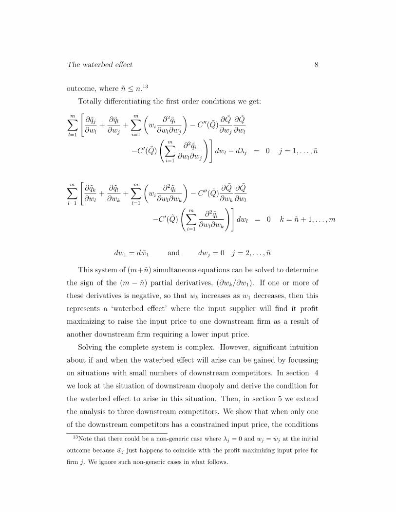
Totally differentiating the first order conditions we get:
m∑l=1
[∂qj∂wl
+∂ql∂wj
+m∑i=1
(wi
∂2qi∂wl∂wj
)− C ′′(Q)
∂Q
∂wj
∂Q
∂wl
−C ′(Q)
(m∑i=1
∂2qi∂wl∂wj
)]dwl − dλj = 0 j = 1, . . . , n
m∑l=1
[∂qk∂wl
+∂ql∂wk
+m∑i=1
(wi
∂2qi∂wl∂wk
)− C ′′(Q)
∂Q
∂wk
∂Q
∂wl
−C ′(Q)
(m∑i=1
∂2qi∂wl∂wk
)]dwl = 0 k = n+ 1, . . . ,m
dw1 = dw1 and dwj = 0 j = 2, . . . , n
This system of (m+n) simultaneous equations can be solved to determine
the sign of the (m − n) partial derivatives, (∂wk/∂w1). If one or more of
these derivatives is negative, so that wk increases as w1 decreases, then this
represents a ‘waterbed effect’ where the input supplier will find it profit
maximizing to raise the input price to one downstream firm as a result of
another downstream firm requiring a lower input price.
Solving the complete system is complex. However, significant intuition
about if and when the waterbed effect will arise can be gained by focussing
on situations with small numbers of downstream competitors. In section 4
we look at the situation of downstream duopoly and derive the condition for
the waterbed effect to arise in this situation. Then, in section 5 we extend
the analysis to three downstream competitors. We show that when only one
of the downstream competitors has a constrained input price, the conditions
13Note that there could be a non-generic case where λj = 0 and wj = wj at the initial
outcome because wj just happens to coincide with the profit maximizing input price for
firm j. We ignore such non-generic cases in what follows.
The waterbed effect 9
for the waterbed effect are simply a natural extension of the duopoly case.
In section 5 we also consider the situation where two of the downstream
competitors have constrained input prices.
4 The case of two downstream firms
Much of the economic insight into the waterbed effect can be derived from
the case of two downstream competitors (m = 2). In this situation, n = 1.
The input supplier faces a binding constraint on the input price it can charge
downstream firm i = 1 but can freely set the input price for downstream firm
i = 2.
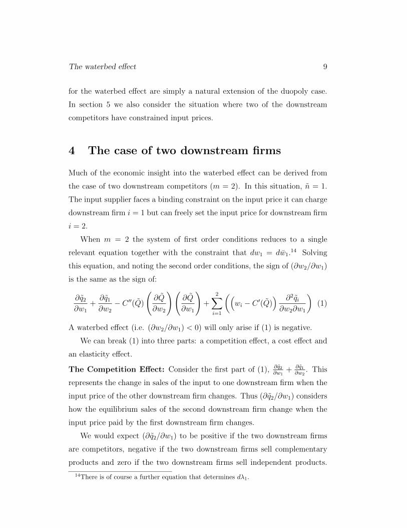
When m = 2 the system of first order conditions reduces to a single
relevant equation together with the constraint that dw1 = dw1.14 Solving
this equation, and noting the second order conditions, the sign of (∂w2/∂w1)
is the same as the sign of:
∂q2∂w1
+∂q1∂w2
− C ′′(Q)
(∂Q
∂w2
)(∂Q
∂w1
)+
2∑i=1
((wi − C ′(Q)
) ∂2qi∂w2∂w1
)(1)
A waterbed effect (i.e. (∂w2/∂w1) < 0) will only arise if (1) is negative.
We can break (1) into three parts: a competition effect, a cost effect and
an elasticity effect.
The Competition Effect: Consider the first part of (1), ∂q2∂w1
+ ∂q1∂w2
. This
represents the change in sales of the input to one downstream firm when the
input price of the other downstream firm changes. Thus (∂q2/∂w1) considers
how the equilibrium sales of the second downstream firm change when the
input price paid by the first downstream firm changes.
We would expect (∂q2/∂w1) to be positive if the two downstream firms
are competitors, negative if the two downstream firms sell complementary
products and zero if the two downstream firms sell independent products.
14There is of course a further equation that determines dλ1.
The waterbed effect 10
Thus, a rise in w1 will tend to raise the equilibrium price p1 and lower equi-
librium sales q1 for firm 1. If firm 2 is a competitor to firm 1 then we would
expect these changes to increase firm 2’s equilibrium sales q2. We would ex-
pect the reverse to occur if firm 2’s product is complementary with firm 1.
The same sign will apply to the other derivative (∂q1/∂w2).
To understand these terms, suppose the two downstream firms compete.
This is the situation most commonly considered for a ‘waterbed’ effect. Then
(∂q2/∂w1) is positive, which acts against a waterbed effect. When the input
price to downstream firm 1 falls, this reduces the ability of the downstream
rival, firm 2, to compete. Given its lower input price, firm 1 will tend to
reduce the price of its downstream product and to increase its level of sales.
From the perspective of the input supplier, the (derived) demand for its
product from firm 2 will fall, reducing the profit-maximizing price that it can
charge firm 2. Thus, the first two terms capture a feedback from a reduction
in the input price paid by one firm through to the profit maximizing input
price charged to its competitive rival.
The competition effect acts against the waterbed effect for competitive
downstream firms. Rather than a fall in the input price to one downstream
firm raising the input price to competitors, the input price to competitors will
also tend to fall. These terms suggest that, to the degree a waterbed effect
exists, it may be relevant for downstream firms that produce complementary
outputs using the same input, not for downstream competitors.
The Cost Effect: The second part of (1), −C ′′(Q)(
∂Q∂w2
)(∂Q∂w1
), represents
the effect on the input supplier’s production costs when output changes as
a consequence of the fall in the input price it can charge downstream firm
1. We would expect (∂Q/∂w1) and (∂Q/∂w2) to both be the same sign so
that, multiplied together, they are positive.15 By assumption, C ′′(Q) ≥ 0.
15Indeed, we would expect each of (∂Q/∂w1) and (∂Q/∂w1) to be negative so that a
reduction in an input price raises total equilibrium output.
The waterbed effect 11
Thus, we expect the total cost effect, as given by −C ′′(Q)(
∂Q∂w2
)(∂Q∂w1
), to
be negative.
The cost effect captures the ‘common intuition’ of the water bed effect.
As one downstream firm is able to reduce the price that it pays for the input,
this will ‘force’ the supplier to raise the input price to other downstream
firms in order to ‘cover its costs’. However, the effect is more subtle than
this ‘common intuition’. It reflects that a reduction in price to one down-
stream firm will increase input sales to that firm, which raises the marginal
production cost to supplying all downstream firms ceteris paribus. Thus the
cost effect operates because a fall in the input price to one firm raises total
sales of the input. Further, it operates because these increased sales involve
an increase in marginal cost. Interestingly, the cost effect operates regardless
of the nature of downstream competition. Thus the cost effect can support
a ‘waterbed effect’ regardless of whether firms compete downstream or not.
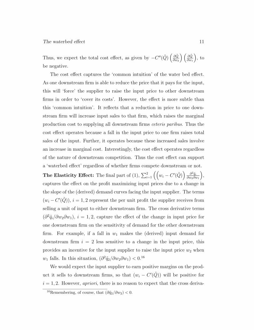
The Elasticity Effect: The final part of (1),∑2
i=1
((wi − C ′(Q)
)∂2qi
∂w2∂w1
),
captures the effect on the profit maximizing input prices due to a change in
the slope of the (derived) demand curves facing the input supplier. The terms
(wi−C ′(Q)), i = 1, 2 represent the per unit profit the supplier receives from
selling a unit of input to either downstream firm. The cross derivative terms
(∂2qi/∂w2∂w1), i = 1, 2, capture the effect of the change in input price for
one downstream firm on the sensitivity of demand for the other downstream
firm. For example, if a fall in w1 makes the (derived) input demand for
downstream firm i = 2 less sensitive to a change in the input price, this
provides an incentive for the input supplier to raise the input price w2 when
w1 falls. In this situation, (∂2q2/∂w2∂w1) < 0.16
We would expect the input supplier to earn positive margins on the prod-
uct it sells to downstream firms, so that (wi − C ′(Q)) will be positive for
i = 1, 2. However, apriori, there is no reason to expect that the cross deriva-
16Remembering, of course, that (∂q2/∂w2) < 0.
The waterbed effect 12
tives (∂2qi/∂w2∂w1), i = 1, 2, will have a particular sign. Rather it will
depend on the nature of downstream interaction.
Discussion of the two-firm case: The case of two downstream firms sheds
significant light on the possibility of a waterbed. The analysis shows that
the waterbed effect can occur and that it has solid economic underpinnings.
Further, it highlights the relevant market factors that policy makers need
to consider when debating both the likelihood and the consequences of the
waterbed effect for particular industries.
For example, the two-firm case highlights that a waterbed effect is more
likely when upstream supply costs are more convex, so if one firm achieves
a lower input price this can lead to higher prices to other firms due to rising
upstream marginal cost. In contrast, if upstream supply involves constant re-
turns to scale technology, the marginal cost of supply does not change for the
input supplier and the ‘cost effect’ is zero. Thus the likelihood of a waterbed
effect depends directly on the nature of the upstream technology. However,
this effect has nothing to do with the nature of downstream competition.
In fact, the two firm case highlights that, to the degree downstream firms
compete, this can militate against the waterbed effect. In such situations,
the ‘competition effect’ is positive. In contrast, the waterbed effect is more
likely if the an input supplier provides the same input to firms that do not
compete or that produce complements. In this situation the competition
effect is either zero or negative.
Indeed, the two-firm case suggests that researchers may have been look-
ing for the waterbed effect in the wrong place. Suppose for example, that the
two downstream firms operate in separate markets. These may be firms that
operate in different countries, or even firms that operate in geographically
seperate parts of the same country. In such a situation, there is no compe-
tition between the firms and we would expect both the competition and the
elasticity effects to be zero (or close to zero). The effect on one downstream

The waterbed effect 13
firm’s input price as a result of a reduction in the other firm’s input price
will depend on the ‘cost effect’. So long as the input supplier faces convex
costs, there will be a waterbed effect, albeit that the size of this effect will
depend on the exact technology.
While the two firm case sheds significant light on the waterbed effect, it
is useful to consider the case of three downstream firms to see if anything
changes.
5 The case of three downstream firms
In this section we consider the case of three downstream firms so that m = 3.
In subsection 5.1 we set n = 1. A fall in w1, lowering the input price for
the first downstream firm, may lead to a profit maximizing increase in the
input price for either of the other two downstream firms. A waterbed effect
will arise if either (∂w2/∂w1) < 0 or (∂w3/∂w1) < 0.
In subsection 5.2 we consider the situation where n = 2 so that a drop
in w1 due to an exogenous tightening of the input price constraint for the
first downstream firm can only lead to a change in the input price facing the
third downstream firm. The second downstream firm’s input price constraint
binds. In this situation, a waterbed effect will arise if (∂w3/∂w1) < 0.
Finally, in subsection 5.3 we consider the situation where n = 2 but there
are linkages between input price constraints, so that a change in w1 can lead
to a change in w2. Again, we consider the implications for a waterbed effect.
5.1 The waterbed effect when there are two uncon-
strained downstream firms
Consider the case where m = 3 and, at the initial equilibrium w0, p0 and q0,
n = 1. We wish to consider the effect of a change in the binding input price
constraint for the first downstream firm, dw1 = dw1. Our interest is in the
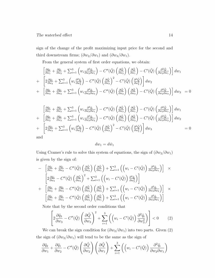
The waterbed effect 14
sign of the change of the profit maximizing input price for the second and
third downstream firms; (∂w2/∂w1) and (∂w3/∂w1).
From the general system of first order equations, we obtain:[∂q2∂w1
+ ∂q1∂w2
+∑3
i=1
(wi
∂2qi∂w2∂w1
)− C ′′(Q)
(∂Q∂w2
)(∂Q∂w1
)− C ′(Q)
(∂2Q
∂w2∂w1
)]dw1
+
[2 ∂q2∂w2
+∑3
i=1
(wi
∂2qi∂w2
2
)− C ′′(Q)
(∂Q∂w2
)2− C ′(Q)
(∂2Q∂w2
2
)]dw2
+[
∂q2∂w3
+ ∂q3∂w2
+∑3
i=1
(wi
∂2qi∂w2∂w3
)− C ′′(Q)
(∂Q∂w2
)(∂Q∂w3
)− C ′(Q)
(∂2Q
∂w2∂w3
)]dw3 = 0
[∂q3∂w1
+ ∂q1∂w3
+∑3
i=1
(wi
∂2qi∂w3∂w1
)− C ′′(Q)
(∂Q∂w3
)(∂Q∂w1
)− C ′(Q)
(∂2Q
∂w3∂w1
)]dw1
+[
∂q3∂w2
+ ∂q2∂w3
+∑3
i=1
(wi
∂2qi∂w3∂w2
)− C ′′(Q)
(∂Q∂w3
)(∂Q∂w2
)− C ′(Q)
(∂2Q
∂w3∂w2
)]dw2
+
[2 ∂q3∂w3
+∑3
i=1
(wi
∂2qi∂w2
3
)− C ′′(Q)
(∂Q∂w3
)2− C ′(Q)
(∂2Q∂w2
3
)]dw3 = 0
and
dw1 = dw1
Using Cramer’s rule to solve this system of equations, the sign of (∂w2/∂w1)
is given by the sign of:
−[
∂q2∂w1
+ ∂q1∂w2− C ′′(Q)
(∂Q∂w2
)(∂Q∂w1
)+∑3
i=1
((wi − C ′(Q)
)∂2qi
∂w2∂w1
)]×[
2 ∂q3∂w3− C ′′(Q)
(∂Q∂w3
)2+∑3
i=1
((wi − C ′(Q)
)∂2qi∂w2
3
)]+
[∂q3∂w2
+ ∂q2∂w3− C ′′(Q)
(∂Q∂w3
)(∂Q∂w2
)+∑3
i=1
((wi − C ′(Q)
)∂2qi
∂w3∂w2
)]×[
∂q3∂w1
+ ∂q1∂w3− C ′′(Q)
(∂Q∂w3
)(∂Q∂w1
)+∑3
i=1
((wi − C ′(Q)
)∂2qi
∂w3∂w1
)]Note that by the second order conditions that2
∂q3∂w3
− C ′′(Q)
(∂Q
∂w3
)2
+3∑
i=1
((wi − C ′(Q)
) ∂2qi∂w2
3
) < 0 (2)
We can break the sign condition for (∂w2/∂w1) into two parts. Given (2)
the sign of (∂w2/∂w1) will tend to be the same as the sign of
∂q2∂w1
+∂q1∂w2
− C ′′(Q)
(∂Q
∂w2
)(∂Q
∂w1
)+
3∑i=1
((wi − C ′(Q)
) ∂2qi∂w2∂w1
)
The waterbed effect 15
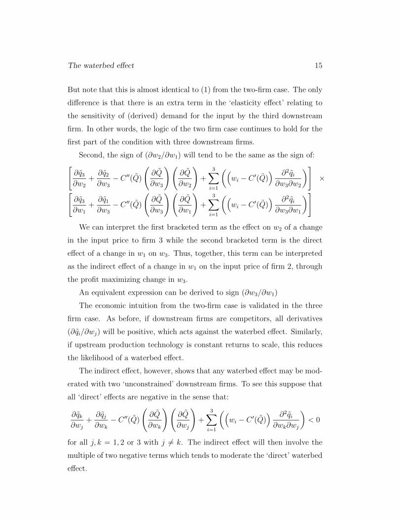
But note that this is almost identical to (1) from the two-firm case. The only
difference is that there is an extra term in the ‘elasticity effect’ relating to
the sensitivity of (derived) demand for the input by the third downstream
firm. In other words, the logic of the two firm case continues to hold for the
first part of the condition with three downstream firms.
Second, the sign of (∂w2/∂w1) will tend to be the same as the sign of:[∂q3∂w2
+∂q2∂w3
− C ′′(Q)
(∂Q
∂w3
)(∂Q
∂w2
)+
3∑i=1
((wi − C ′(Q)
) ∂2qi∂w3∂w2
)]×[
∂q3∂w1
+∂q1∂w3
− C ′′(Q)
(∂Q
∂w3
)(∂Q
∂w1
)+
3∑i=1
((wi − C ′(Q)
) ∂2qi∂w3∂w1
)]We can interpret the first bracketed term as the effect on w2 of a change
in the input price to firm 3 while the second bracketed term is the direct
effect of a change in w1 on w3. Thus, together, this term can be interpreted
as the indirect effect of a change in w1 on the input price of firm 2, through
the profit maximizing change in w3.
An equivalent expression can be derived to sign (∂w3/∂w1)
The economic intuition from the two-firm case is validated in the three
firm case. As before, if downstream firms are competitors, all derivatives
(∂qi/∂wj) will be positive, which acts against the waterbed effect. Similarly,
if upstream production technology is constant returns to scale, this reduces
the likelihood of a waterbed effect.
The indirect effect, however, shows that any waterbed effect may be mod-
erated with two ‘unconstrained’ downstream firms. To see this suppose that
all ‘direct’ effects are negative in the sense that:
∂qk∂wj
+∂qj∂wk
− C ′′(Q)
(∂Q
∂wk
)(∂Q
∂wj
)+
3∑i=1
((wi − C ′(Q)
) ∂2qi∂wk∂wj
)< 0
for all j, k = 1, 2 or 3 with j 6= k. The indirect effect will then involve the
multiple of two negative terms which tends to moderate the ‘direct’ waterbed
effect.
The waterbed effect 16
If the ‘direct’ effects are all negative, so a reduction in w1 tends to raise
the profit maximizing input price for downstream firm i = 2 and i = 3, then
as w3 rises the waterbed effect starts to operate in reverse on w2. The rise in
w3 tends to moderate the size of any rise in w2 and vice versa. Of course, our
analysis here cannot determine the absolute size of (∂w2/∂w1) or (∂w3/∂w1)
- that would require specific numerical analysis.
In summary, when there are multiple unconstrained downstream firms,
the logic of the waterbed effect for the two-firm case continues to hold. How-
ever, there are offsetting indirect effects that will interact with the direct
effects. In particular, if all downstream firms face a ‘direct’ waterbed effect,
then the indirect effects will act to offset the direct effects.
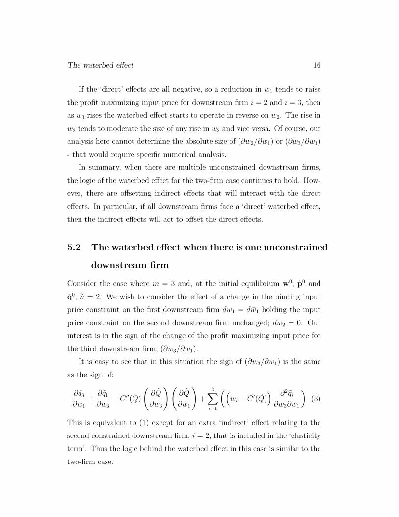
5.2 The waterbed effect when there is one unconstrained
downstream firm
Consider the case where m = 3 and, at the initial equilibrium w0, p0 and
q0, n = 2. We wish to consider the effect of a change in the binding input
price constraint on the first downstream firm dw1 = dw1 holding the input
price constraint on the second downstream firm unchanged; dw2 = 0. Our
interest is in the sign of the change of the profit maximizing input price for
the third downstream firm; (∂w3/∂w1).
It is easy to see that in this situation the sign of (∂w3/∂w1) is the same
as the sign of:
∂q3∂w1
+∂q1∂w3
− C ′′(Q)
(∂Q
∂w3
)(∂Q
∂w1
)+
3∑i=1
((wi − C ′(Q)
) ∂2qi∂w3∂w1
)(3)
This is equivalent to (1) except for an extra ‘indirect’ effect relating to the
second constrained downstream firm, i = 2, that is included in the ‘elasticity
term’. Thus the logic behind the waterbed effect in this case is similar to the
two-firm case.
The waterbed effect 17
5.3 The waterbed effect when input price constraints
are linked
Finally, it is possible that there may be links between the input price con-
straints facing the upstream supplier. For example, a tightening of the input
price constraint relating to downstream firm i = 1 may also alter an input
constraint relating to another downstream firm.
Input price constraints could be linked for a variety of reasons. For exam-
ple, two downstream firms may be able to (legally) enter an agreement that
provides them with the option of jointly establishing an alternative source of
supply that would be uneconomic for either downstream firm by themselves.
In this situation, the price constraint faced by the upstream supplier when
setting input prices for either of these downstream firms will tighten due to
the agreement.
Alternatively, constraints may move in opposite directions. For example,
if one downstream firm merges with a vertically integrated firm in a different
country, this may enhance its own option of gaining alternative input supply,
but may make the threat of input supply to other downstream firms from
the vertically integrated company less credible.
To analyze this situation, consider the case where m = 3 and at the
initial equilibrium w0, p0 and q0, n = 2. We wish to consider the effect of
a change in the binding input price constraint on the first downstream firm
dw1 = dw1 that is connected to the change in the input price constraint on the
second downstream firm. Thus, dw2 = δdw1 where δ can be either positive
or negative. Clearly the case with δ = 0 is identical to subsection 5.2 above.
Again, our interest is in the sign of the change of the profit maximizing input
price for the third downstream firm; (∂w3/∂w1).
Solving the system of first-order equations in this case we see that the
The waterbed effect 18
sign of (∂w3/∂w1) is the same as the sign of:[∂q3∂w1
+ ∂q1∂w3− C ′′(Q)
(∂Q∂w3
)(∂Q∂w1
)+∑3
i=1
((wi − C ′(Q)
)∂2qi
∂w3∂w1
)](4)
+ δ[
∂q3∂w2
+ ∂q2∂w3− C ′′(Q)
(∂Q∂w3
)(∂Q∂w2
)+∑3
i=1
((wi − C ′(Q)
)∂2qi
∂w3∂w2
)]The first part of (4) is equivalent to (3). It gives the direct effect on w3 due
to the change in w1. The second part of (4) represents the effect on w3 due to
a change in w2. It is weighted by δ to reflect the link between the change in
w1 and the change in w2. Depending on the sign of δ, the linking of the two
price constraints can exacerbate or reduce any waterbed effect that arises
when w1 falls.
Finally, there is of course a waterbed effect on downstream firm 2 when-
ever δ is negative. In this situation, a fall in w1 will change the constraint
on the second downstream firm allowing the input supplier to raise the price
to this downstream firm.
In our model any linking of constraints is exogenous. However, as dis-
cussed in section 1, this linkage plays a key role in the analysis of the waterbed
effect, for example, by Inderst and Valletti (2011).
While a price change that arises due to linkage between pricing constraints
may be of interest in its own right, in our opinion, the key argument about
the waterbed effect has arisen where such linkage is absent. In particular the
debate has focussed on small firms (such as small retailers) who have little if
any outside option for an input, and how their input prices will alter when
a larger firm is able to exert buyer power on the relevant input supplier. As
such, our model has focused on these situations and highlighted if, and when,
such small firms will face a rise in their input prices.
6 Conclusion
This paper has presented a simple but parsimonious model to analyse the re-
lationship between countervailing power and downstream pricing. We have
The waterbed effect 19
focussed on situations where one downstream firm has increased counter-
vailing power that enables it to gain a lower input price from an upstream
supplier. Our focus has been on the effect of such a change on the profit
maximizing prices that the supplier sets for other downstream firms. In par-
ticular, we have considered whether or not a waterbed effect could arise:
where a reduction in one downstream firm’s input price due to increased
countervailing power results in a higher input price to one or more of the
other downstream firms.
Our model has shown that the presence or absence of any waterbed effect
will depend on the interplay of three interrelated changes. First, a waterbed
effect is less likely to arise when a downstream firm is a competitor to the
firm that has increased its countervailing power. This ‘competition effect’
arises because a lower input price for one downstream firm moderates the
input demand of its competitors. In contrast, if downstream firms use the
same input to produce complementary products, then a waterbed effect is
more likely.
Second, a waterbed effect is more likely when upstream production costs
are convex. Increased countervailing power for one downstream firm means
that this firm receives a lower input price and purchases more of the input.
But with convex production costs, the increase in sales of the input tends to
raise the marginal cost for the input supplier. This, in turn, raises the profit
maximizing price the supplier will set for all other downstream firms.
Importantly, this ‘cost effect’ does not depend on downstream competi-
tion or complementarity. It arises whenever the downstream firms buy the
same input and production costs for the input are convex. Thus an ‘indepen-
dent’ downstream firm, in a different location or market to the downstream
firm with increased countervailing power, could face a ‘waterbed effect’ due
to the convexity of upstream costs.
Third, a change in the input price paid by one downstream firm can lead
to changes in the elasticity of input demand for other downstream firms.
The waterbed effect 20
These changes can lead to a rise or fall in the profit maximizing price that the
supplier sets for the relevant downstream firms. It could lead to a ‘waterbed
effect’, or the reverse. Without knowing the details of downstream demand,
the influence of this ‘elasticity effect’ is ambiguous.
This paper is complementary to other papers that have considered the
waterbed effect. This other work has focussed on price changes that originate
from ‘links’ between bargaining outcomes. In other words, these papers have
considered situations where multiple downstream firms have countervailing
power and a change in the countervailing power for one downstream firm has
implications for the countervailing power of other downstream firms. Our
model is able to include such links, so that an increase in countervailing
power for one downstream firm can directly effect the price constraint that
the supplier faces for another downstream firm. However, in our model such
linkages are ‘black boxed’. Other work has considered how and why these
linkages can arise.
In contrast, this paper focuses on input price changes for firms that have
no countervailing power. In this sense, our model captures some of the con-
cerns expressed in the public debate on the waterbed effect, where the fear
is that countervailing power exercised by one or more ‘large’ downstream
firms will lead to higher input prices for small downstream firms that have
no countervailing power.17
The model presented in this paper provides useful guidance for policy
makers concerned about the ‘waterbed effect’. For example, if downstream
firms are strong competitors, upstream production technology is constant
returns to scale and final consumers are ‘similar’, so that significant changes
in the elasticity of the derived input demand are unlikely, then a ‘waterbed
effect’ is unlikely.18
17Of course, the model presented in this paper does not require size to be associated
with countervailing power.18The caveat here is that a waterbed effect may arise through linkages in bargaining
The waterbed effect 21
In contrast, a waterbed effect is more likely when upstream production
is characterized by capacity constraints or highly convex costs. But this
effect on input prices reflects the need for the input supplier to ration output
among downstream firms. It is independent of the nature of downstream
interaction.
Indeed, the model presented in this paper suggests that policy makers may
have been looking for the waterbed effect in the wrong place. Downstream
competition militates against the waterbed effect. Thus, a waterbed effect
may be more likely where downstream firms operate in different markets or
sell complementary products.
References
Chipty, T. and C.M. Snyder, (1999), “The role of firm size in bilateral bar-
gaining: a study of the cable television industry”, Review of Economics
and Statistics, 81, 326-340.
Competition Commission (2008) The supply of groceries in the UK market
investigation, 30 April, www.competition-commission.org.uk
European Commission (2001) “Guidelines on the applicability of Article
81 of the EC Treaty to hosrizontal cooperation agreements”, Official
Journal of the European Communities, 2001/C 3/02.
Galbraith, J.K. (1952) American Capitalism: The Concept of Countervail-
ing Power. Boston: Houghton Mifflin.
Inderst, R. (2007) “Leveraging buyer power, International Journal of In-
dustrial Organization, 25, 908-924.
constraints. As noted, the model presented here complements the existing literature that
considers these linkages.
The waterbed effect 22
Inderst, R. and T. Valletti (2011) “Buyer power and the ‘waterbed effect”’,
The Journal of Industrial Economics, 59, 1-20.
Inderst, R. and C. Wey, (2003) “Bargaining, mergers, and technology choice
in bilaterally oligopolistic industries”, RAND Journal of Economics,
34, 1-19.
Inderst, R. and C. Wey, (2007) Buyer power and supplier incentives, Euro-
pean Economic Review, 51, 647-667.
Katz, M.L. (1987) “The welfare effects of third degree price discrimination
in intermediate goods markets”, American Economic Review, 77, 154-
167.
Majumdar, A. (2005) “Waterbed effects and buyer mergers”, CCP Working
Paper 05-7, University of East Anglia.
Snyder, C.M. (2008) “Countervailing power”, in The New Palgrave Dictio-
nary of Economics, 2nd. Edition, S.N. Durlauf and L.E. Blume (eds)
Palgrave Macmillan.


