Report EUR 27494 EN

Andreas Dietzel, Joachim Maes

2015

Costs of restoration measures in the EU based on an assessment of LIFE projects

European Commission

Joint Research Centre

Institute for Environment and Sustainability

Contact information

Joachim Maes

Address: Joint Research Centre, Via Enrico Fermi 2749, 21027 Ispra (VA), Italy

E-mail: joachim.maes@jrc.ec.europa.eu

Tel.: +39 0332 78.91.48

JRC Science Hub

https://ec.europa.eu/jrc

Legal Notice

This publication is a Technical Report by the Joint Research Centre, the European Commission’s in-house science service.

It aims to provide evidence-based scientific support to the European policy-making process. The scientific output

expressed does not imply a policy position of the European Commission. Neither the European Commission nor any person

acting on behalf of the Commission is responsible for the use which might be made of this publication.

All images © European Union 2015)

JRC97635

EUR 27494 EN

ISBN 978-92-79-52208-6 (PDF)

ISSN 1831-9424 (online)

doi:10.2788/235713

Luxembourg: Publications Office of the European Union, 2015

© European Union, 2015

Reproduction is authorised provided the source is acknowledged.

Abstract

Restoring ecosystems to reverse biodiversity loss and to enhance ecosystem services is an important target of the EU

Biodiversity Strategy to 2020. At global and European level the target is to restore 15% of degraded ecosystems.

Identifying sites that should be considered for restoration in order to achieve the target requires spatial information on

where degraded ecosystem are, on the kind of mitigation measures that are needed to restore ecosystems to a good

condition, and on the costs and benefits of restoration in order to prioritise investments. At all these levels, detailed spatial

information is lacking. This report contributes to the ecosystem restoration knowledge base by providing cost estimates of

specific restoration measures.

Costs of restoration measures in the EU based on an assessment of LIFE projects

2

Contents

Contents ................................................................................................................................................................................ 2

Acronyms ............................................................................................................................................................................. 3

Executive Summary ......................................................................................................................................................... 4

1 Introduction .............................................................................................................................................................. 6

2 Material and Methods ........................................................................................................................................... 8

2.1 The LIFE database ......................................................................................................................................... 8

2.2 Restoration typology ................................................................................................................................... 9

2.3 Budget standardization ........................................................................................................................... 11

2.4 Multiple linear regression ...................................................................................................................... 12

2.4.1 Non-negative least squares (NNLS) .......................................................................................... 12

2.4.2 MS Excel’s Solver .............................................................................................................................. 14

2.4.3 Economy of scale .............................................................................................................................. 14

2.4.4 Solving methods ................................................................................................................................ 15

3 Results ...................................................................................................................................................................... 16

3.1 Frequency analyses ................................................................................................................................... 16

3.2 Cost estimation ............................................................................................................................................ 17

3.2.1 SOLVER ................................................................................................................................................. 17

3.2.2 NNLS ...................................................................................................................................................... 19

4 Discussion ............................................................................................................................................................... 23

4.1 Cost estimates .............................................................................................................................................. 23

4.2 Comparison of regression methods NNLS and SOLVER ............................................................ 24

4.3 Cost estimates of individual measures .............................................................................................. 24

4.4 Budget allocation ........................................................................................................................................ 25

4.5 Conclusion ..................................................................................................................................................... 25

5 References ............................................................................................................................................................... 26

6 Appendix.................................................................................................................................................................. 27

3

Acronyms

CLC Corine Land Cover

EC European Commission

ETC/BD European Topic Centre on Biological Diversity

EU European Union

EUNIS European Nature Information System classification

HICP Harmonized Indices of Consumer Prices

NGO Non-Governmental Organisation

NUTS Nomenclature of Territorial Units for Statistics

PLI Price Level Index

4

Executive Summary

Restoring ecosystems to reverse biodiversity loss and to enhance ecosystem services is an

important target of the EU Biodiversity Strategy to 2020. At global and European level the target

is to restore 15% of degraded ecosystems. Identifying sites that should be considered for

restoration in order to achieve the target requires spatial information on where degraded

ecosystem are, on the kind of mitigation measures that are needed to restore ecosystems to a

good condition, and on the costs and benefits of restoration in order to prioritise investments.

At all these levels, detailed spatial information is lacking. This report contributes to the

ecosystem restoration knowledge base by providing cost estimates of specific restoration

measures.

The cost estimates are based on an analysis of Life Nature projects. Life is the name of the main

EU funding instrument for the environment. In this analysis, Life projects classified under the

strand ‘Nature’ were considered since these projects target restoration activities in Natura 2000

sites. Although project reports differ in quality and level of detail, the LIFE database constitutes

a valuable source of information on ecosystem restoration across the EU presented in a

standardized format.

We adopted and refined a restoration measure classification system developed by Benayas,

Newton, Diaz, & Bullock (2009) through an initial screening process of Life project reports. The

resulting restoration typology discriminated between 23 different restoration measures. Next

215 Life Nature projects were selected for a more in-depth analysis of different the restoration

actions. For every project the total budget was known. Where possible restoration activities

were quantified using length, area or mass based units. If quantification was not possible,

restoration activities were recorded using presence or absence on a project basis. We then

conducted a series of multiple regression analyses to provide cost confidence intervals for 15

restoration measures so that the sum of cost of all restoration measures taken per project

equalled the total project budget. In the analysis we considered overhead costs as well as

economy of scale effects.

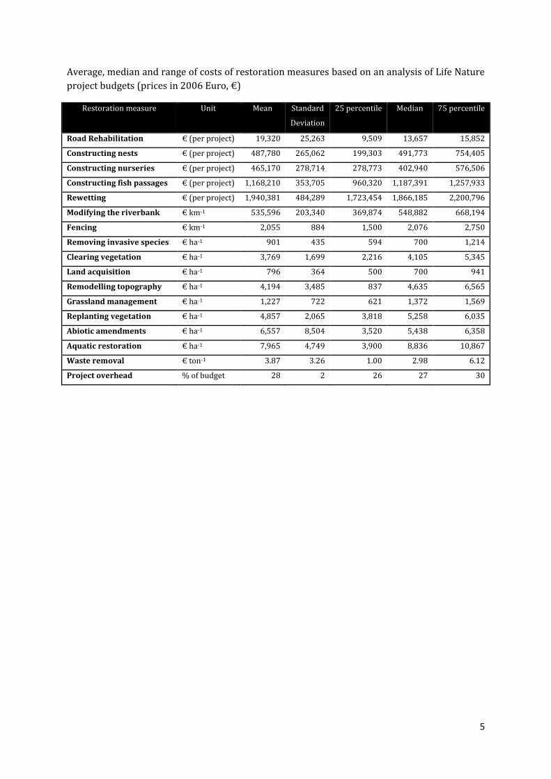
A summary of the best available information with cost estimates per restoration measure is

presented in the summary table.

Despite the high variance in cost estimates the presented cost confidence intervals and average

unit costs with standard deviation this report provides a usable approximation of actual

restoration costs for the assumptions we made. Although the high variance may preclude them

from being used for fine-grain analysis such as cost predictions on a project basis, we are

confident that cost ranges may prove useful for more coarse-grain analysis such as the

prediction of restoration expenditures at national or EU level given certain biodiversity

conservation or restoration targets. For such meta-analysis purposes the upper and lower

bounds of the cost confidence intervals can be used to provide a range of expected restoration

expenditures.

5

Average, median and range of costs of restoration measures based on an analysis of Life Nature

project budgets (prices in 2006 Euro, €)

Restoration measure Unit Mean Standard

Deviation

25 percentile Median 75 percentile

Road Rehabilitation € (per project) 19,320 25,263 9,509 13,657 15,852

Constructing nests € (per project) 487,780 265,062 199,303 491,773 754,405

Constructing nurseries € (per project) 465,170 278,714 278,773 402,940 576,506

Constructing fish passages € (per project) 1,168,210 353,705 960,320 1,187,391 1,257,933

Rewetting € (per project) 1,940,381 484,289 1,723,454 1,866,185 2,200,796

Modifying the riverbank € km-1 535,596 203,340 369,874 548,882 668,194

Fencing € km-1 2,055 884 1,500 2,076 2,750

Removing invasive species € ha-1 901 435 594 700 1,214

Clearing vegetation € ha-1 3,769 1,699 2,216 4,105 5,345

Land acquisition € ha-1 796 364 500 700 941

Remodelling topography € ha-1 4,194 3,485 837 4,635 6,565

Grassland management € ha-1 1,227 722 621 1,372 1,569

Replanting vegetation € ha-1 4,857 2,065 3,818 5,258 6,035

Abiotic amendments € ha-1 6,557 8,504 3,520 5,438 6,358

Aquatic restoration € ha-1 7,965 4,749 3,900 8,836 10,867

Waste removal € ton-1 3.87 3.26 1.00 2.98 6.12

Project overhead % of budget 28 2 26 27 30

6

1 Introduction

Centuries of land transformation, industrialisation, urbanisation and agricultural intensification

have left their scars on Europe’s landscape, with devastating effects for its species and habitats

(e.g. MEA, 2005). In an attempt to halt and reverse these trends, the European Commission (EC)

adopted the Birds Directive and the Habitats Directive, which since their establishment in 1979

and 1992 respectively have formed the backbone of nature conservation policy in the European

Union (EU).

The EU has set itself the ambitious target of halting biodiversity loss by 2020 (formerly 2010)

and beyond. To monitor the envisioned improvements in biodiversity conservation, a large-

scale monitoring scheme has been set in place obligating every member state to periodically

conduct biodiversity surveys and report on the conservation status of those habitats and

species considered to be of European interest (listed in Annexes 1 and 2 of the Habitats

Directive). The results of the first survey conducted between 2001 and 2006 revealed that the

majority of habitat (65%) and species (52%) assessments recorded an unfavourable

conservation status. A second survey round, reporting for the period between 2006 and 2012

confirms by large these findings and paint a dire picture of the state of Europe’s habitats and

species. Conservation policies should go beyond the mere preservation of the status-quo and

instigating the large-scale restoration of degraded habitats.

The restoration of degraded ecosystems is known to be effective in enhancing ecosystem

services and reversing biodiversity loss (Bullock, Aronson, Newton, Pywell, & Rey-Benayas,

2011; Rey Benayas, Newton, Diaz, & Bullock, 2009) and is regarded as a cornerstone of the EU’s

endeavours to reach its biodiversity conservation targets. The LIFE programme, launched in

1992, provides the necessary financial incentives. Besides projects on innovative environmental

policy approaches and information and communication campaigns LIFE has co-financed about

1400 best practice and demonstration projects of species and habitat conservation (LIFE

Nature) throughout Europe. LIFE Nature projects have targeted a wide variety of species and

habitats, have sought to mitigate a diverse set of anthropogenic pressures and have been

carried out all over Europe. Project reports specifying, amongst others, the restoration

objectives and results are stored in the LIFE database and publicly available.

Harvesting the wealth of practical restoration experience for policy-making purposes and to

advance restoration science is a major challenge often neglected (Menz, Dixon, & Hobbs, 2013;

Suding, 2011). Inherent problems of restoration science include the lack of replicates and clear

boundaries, especially in terrestrial and marine ecosystems, or the heterogeneity of sites and

methods (Weiher, 2007). Limited monitoring, restricted access to monitoring data and a lacking

consensus on standard evaluation criteria further exacerbate the generalizability of practical

insights into ecosystem restoration activities (Suding, 2011). Although project reports differ in

quality and level of detail, the LIFE database constitutes a valuable source of information on

ecosystem restoration in the EU presented in a standardized format. Few studies have, however,

attempted to translate this piecemeal information into more general, scientific findings.

In this study, we harnessed the wealth of information stored in the LIFE database to draw

conclusions about one of the major knowledge gaps of ecosystem restoration in the EU, the

costs of restoration activities. Information on the costs of ecosystem restoration activities is

sparse and inconsistent (e.g. Bernhardt et al., 2005) and thus difficult to use for policy-making

7

purposes at the EU level. Insights into restoration costs could be used for a variety of purposes

such as benchmarking restoration projects or efficient budget allocation. When combined with

an economic evaluation of the impact of restoration activities on ecosystem service supply, cost

estimates can also be consulted for cost-benefit analyses on the economic viability of

restoration projects (De Groot et al., 2013). Acuña et al. (2013), for instance, investigated

whether the benefits of restoring rivers by adding dead wood outweighed the costs accrued.

Putting a price tag on restoration activities would, however, not only prove useful for informing

decision making at project but also at member state and EU level, especially when faced with the

challenge of up-scaling demonstration projects to the ecologically more meaningful landscape

level (Menz et al., 2013). At the national and supranational level cost estimates could be used to

set restoration priorities or calculate the cost implications of the EU’s biodiversity targets,

which, amongst others, stipulate that by 2020 at least 34 per cent of the habitat assessments

will report a favourable or significantly improved conservation status (The EU biodiversity

strategy to 2020).

LIFE restoration projects have targeted a wide variety of species, habitats and anthropogenic

pressures. Adding to that the wide gaps in e.g. labour costs and land prices that prevail between

member states, we get a good picture of the difficulties encountered when trying to generalize

restoration costs over a “study area” as economically and ecologically heterogeneous as Europe.

For this, we screened the LIFE database for projects providing a detailed and quantified account

on restoration activities, filled data gaps by approximating quantities and calculated average

costs for the most frequently applied measures through a regression analysis.

8

2 Material and Methods

2.1 The LIFE database

The LIFE programme is the European Union’s financial instrument for fostering environmental

and nature conservation. Since 1992, in 4 consecutive phases, €3.1 billion has been conceded to

co-finance about 4000 projects in the categories Nature & Biodiversity (formerly LIFE Nature),

Environment Policy & Governance (formerly LIFE Environment) and Information &

Communication (since LIFE+, phase 4). The LIFE strand Nature (& Biodiversity) comprises

more than 1400 best practice and demonstration projects that contribute to the implementation

of the EU’s Birds and Habitats Directives and to the establishment of the Natura 2000 network.

Project beneficiaries cover the whole spectrum of public and private actors and include,

amongst others, national, regional and local public authorities, non-governmental organisations

(NGO), research institutions and enterprises. Short reports indicating the background,

objectives and results constitute one of the project deliverables and have been made publicly

available on the LIFE website. Although information quality and level of detail vary between

project reports, the LIFE database exhibits a great source of concise information on ecosystem

restoration projects in the European Union.

To give an overview of the content of the LIFE database we conducted a series of simple

frequency analyses including 1409 LIFE Nature projects which were registered between 1992

and 2011. We assessed the following information:

the main beneficiaries of the LIFE program,

the frequency of targeted broad taxonomic (amphibians, birds, fish, invertebrates,

mammals, plants and reptiles) and habitat groups (coastal and halophytic habitats,

coastal sand dunes and inland dunes, forests, freshwater habitats, raised bogs and mires

and fens, rocky habitats and caves, sclerophyllous scrub, temperate heath and scrub,

natural and semi-natural grassland formations) and

patterns in LIFE budget allocation (over taxonomic and habitat groups and over NUTS-

1 regions)

The budget of projects targeting more than one habitat, species or region was assumed to be

equally distributed over target habitats, species and regions.

For the geographical distribution analysis, budgets were standardized following the procedure

explained in section 2.3 accounting for differences in economic development between member

states and over time. Only projects between the years 1996 and 2011 were considered as for

earlier projects data on economic indicators used for the budget standardization was not

available. To account for different entry dates of member states to the EU, budget allocation was

mapped for different time horizons (1996-2011, 2004-2011, and 2007-2011). The years 2004

and 2007 were chosen as milestones in the eastward expansion of the EU with ten (Cyprus,

Czech Republic, Estonia, Hungary, Latvia, Lithuania, Malta, Poland, Slovakia, and Slovenia)

countries joining the EU in 2004 and two more (Bulgaria and Romania) in 2007.

The budget allocation maps were visually compared to maps of population density, number of

Article 17 species (all at NUTS-1 level) and the proportion of artificial land cover (NUTS-level 0)

to draw conclusions about potential geographic patterns in budget allocation. Data on

9

population density (reference year 2006) and artificial land cover (reference year 2009) was

retrieved from the EU’s statistical office Eurostat. The diversity of Article 17 species per region

was calculated by intersecting species distribution maps (as reported during the Article 17 of

the Habitats Directive (92/43/EEC) covering the period 2001 to 2006) with the NUTS regions. A

species was considered to be present in a respective NUTs region if at least one raster cell

(resolution 10x10km) at least partially overlapped with the respective NUTs polygon.

2.2 Restoration typology

The purpose of this study was to derive cost estimates of the most frequently applied

restoration measures from the wealth of information contained in the LIFE database. For this,

we adopted and refined a restoration measure classification system developed by Benayas,

Newton, Diaz, & Bullock (2009) through an initial screening process of LIFE project reports.

The resulting restoration typology (table 1) discriminates between 23 different measure classes

and was subsequently used to retrieve for each of the LIFE Nature project reports examined in

this study the measures applied and corresponding quantities (e.g. the total area of habitat

restored, fenced or put under extensive grazing). Records lacking quantified information were

treated as binary (presence-absence) data, for instance the construction of a fish ladder to

restore the connectivity of a stream.

There was no consistency in the project files of the database when reporting on the different

restoration actions taken in the project. Some projects just list certain restoration actions

whereas other projects provide more detail. Restoration actions are quantified using unit area

(ha), unit length (km) in case of actions along rivers, roads or in case of placing fences, or unit

mass (ton) in case of removal of sediment or waste (table 1). Some restoration measures are

hard to quantify in any of these units and were quantified as present or absent (yes/no, table 1)

and treated as a binary variable in subsequent analysis. Semi-quantitative information was

converted into presence or absence of a measure. Some projects did not provided estimates of

restoration actions which are quantified in units area, length or mass in table 1. In the statistical

analysis these records were given either the median value based on all positive records within

the same restoration measure, or the maximum value of all restoration actions within the same

project, or whichever of these two values is the smallest.

In order to reduce the number of explanatory variables in the dataset, we omitted some less

frequently recorded restoration measures and merged similar restoration measures. Table 1

gives an overview of the revision of the classification scheme. For statistical reasons, we

harmonized measures containing records with different dimensions (e.g. surface area and

length) applying the assumptions listed in table 2.

10

Table 1. Measure reclassification scheme showing how measure classes were regrouped,

merged or dropped after the initial screening of the database.

Original classification Unit Final classification

AQUATIC RESTORATION

River flow modification km Aquatic Restoration

Restoration of water bodies (ponds, streams) ha

Rewetting/raising of groundwater table ha Rewetting

Fish passages yes/no Fish Passages

Bank modifications/stabilization km Bank Modification

VEGETATION RESTORATION

Planting of forbs or grasses ha Replanting vegetation

Planting of trees and shrubs ha

Reinstatement of burning ha Burning Vegetation

Removal of vegetation (single event) ha Clearing Vegetation

Grazing or mowing ha Grassland Management

OVERHEAD

Cessation of degrading action only (passive) yes/no Passive restoration

Tourist infrastructure yes/no Tourist Infrastructure

Others yes/no Others

Establishment of seed banks yes/no -

OTHERS

Extirpation of damaging/invasive species ha Invasive Species

Artificial nests yes/no Nesting sites

Nursery and release yes/no Nursery

Restrict access to humans and animals km Fencing

Road rehabilitation km Road Rehabilitation

Removal of infrastructure, rubbish, sediment tonne Waste Removal

Land acquisition/compensation/material ha Land Acquisition

Remodelling of topography ha Remodelling topography

Nutrient removal or enrichment yes/no Abiotic amendments

11

Table 2: Assumptions applied to harmonize restoration measures with different dimensions.

Restoration measure Value Unit

Width of riparian vegetation 10 m

Width of road 5 m

Width of river 10 m

Width of dune/dyke 50 m

Width of hedge 5 m

Width ditch 2 m

Density of trees planted 1750 ha-1

Density of cranberries planted 2500 ha-1

Density of shrubs planted 5 m-2

Weight of soil 1.6 t m-3

Volume of one truck load 10 m3

Depth of sod cutting 0.1 m

Dredging depth of top soil/silt/sediment removed 0.5 m

Average size of pond 0.5 ha

Average size of pool 50 m2

Thinning forest/cutting whole forest 10 %

Decaying wood/cutting whole forest 5 %

Fence length per ha 0.4 km ha-1

2.3 Budget standardization

The prevalent disparities in the economic development of EU member states presuppose a

budget standardization procedure that accounts for differences in restoration costs between

countries and over time. We used the indicators Harmonized Indices of Consumer Prices (HICP)

and Price Level Index (PLI) from Eurostat (cf. appendix A) to let all project budgets reflect 2006

€ levels (HICP) at an EU-average level of economic development (PLI). The definition of the two

economic indicators is given below.

Definitions of economic indicators

Price Level Index (PLI) The price level index, abbreviated as PLI, expresses the price level of a given country relative to another (or relative to a group of countries like the European Union), by dividing the Purchasing power parities (PPPs) by the current nominal exchange rate.

Harmonized Indices of Consumer Prices (HICP)

The HICPs are economic indicators constructed to measure the changes over time in the prices of consumer goods and services acquired by households. The HICPs give comparable measures of inflation in the euro-zone, the EU, the European Economic Area and for other countries including accession and candidate countries. They are calculated according to a harmonised approach and a single set of definitions.

12

2.4 Multiple linear regression

The goal of this study was to extract cost estimates of restoration measures which were most

frequently applied throughout the LIFE program based a sample of 215 restoration projects

with detailed accounts of stated project budgets, applied measures and their quantities. For this,

we constructed a multiple linear regression analysis to solve the system

where the regression coefficients (𝛃0, 𝛃1, ……… , 𝛃p) correspond to the cost estimates of each

measure p per unit, xnp corresponds to the reported quantities of each measure applied in

project n and y to the predicted project budgets. Recall that reported quantities can either take

continuous or binary values. We used the ordinary least squares (OLS) optimization approach to

solve this over-constrained (i.e. more constraints/equations than explanatory

variables/measures) system and to find sets of regression coefficients that best predict stated

project budgets. We followed two different approaches to multiple OLS regression, the R

package non-negative-least-squares (NNLS) and a manual solution involving MS Excel’s SOLVER

function, and compared their suitability for extracting reasonable cost estimates from our

dataset.

For both methods, the optimization rule uses the sum of least squares approach which reads as

min𝑥∑(𝑃𝑗 − 𝑆𝑗)

2

𝑛

𝑗=1

where n is the number of projects, Pj is the predicted budget and Sj is the stated budget of

project j.

2.4.1 Non-negative least squares (NNLS)

The NNLS package (Version 1.4) is an R interface to the Lawson-Hanson implementation of an

algorithm for non-negative least squares that allows for constraining regression outputs to non-

negative and non-positive values. It solves the least squares problem min ||Ax = b ||2 with the

constraint x ≥ 0 where x ∈ Rn; b ∈ Rm and A in an m x n matrix (Lawson and Hanson, 1995). The

constraint is necessary to avoid negative values for restoration measures.

NNLS runs were performed in RStudio (Version 0.97.551) for different versions of the original

dataset. Versions differed in the number of measures and projects included and were derived by

a) a step-wise elimination of the less frequently recorded measures,

b) regrouping/merging similar measure classes

13

c) using only projects with a certain minimum number of measures applied.

The restoration measure classes Others, Tourist Infrastructure and Passive (table 1) were

excluded from all runs and were, together with labour and administrative costs, accounted for

as Overhead expenditures. Overhead costs were assumed to consume about twenty per cent of

overall budgets in the NNLS approach. An overview over the specifications of the different NNLS

runs is given in Table 3.

Table 3. Overview if specifications of NNLS regression analysis runs with N(project) indicating

the number of projects included in the run, N(measure) the amount of measure classes included

and Nmin (measures per project) the minimum number of applied measures for a project to be

included in the analysis.

Dataset N (project) N (measure) Dropped measures Nmin (measures per project)

OR raw 25 - -

OR ref 215 25 - -

A1 215 17 Tourist Inf, Passive, Others -

A2 198 17 - 2

A3 177 17 - 3

A4 130 17 - 4

A5 82 17 - 5

A6 202 16 Road -

A7 185 16 Nurse -

A8 199 16 Nests -

A9 202 16 Burn -

A10 206 16 Abiotic -

B1 156 13 Nurse, Nests, Burn, Road, Abiotic -

B2 140 13 - 2

B3 122 13 - 3

B4 84 13 - 4

C1 179 11 {Burn & Clear Veg} and {Shore Mod & Topo}

-

C2 158 11 - 2

C3 127 11 - 3

For each NNLS output, we calculated the median, the minimum and maximum values, the first

and third quartile and the average of all non-zero values to provide a cost confidence range for

each restoration measure. The goodness-of-fit between stated project budgets and budgets

predicted using the derived cost estimates per measure was tested using MS Excel’s LINEST

function. LINEST offers an OLS-curve-fitting routine that calculates trend line statistics and

corresponding uncertainties (slope, standard error of slope, intercept, standard error of

intercept, R2, F statistics, degrees of freedom and regression sum of squares and residual sum of

squares). The Intercept 𝛃0 was set to zero and the goodness-of-fit was assessed on the basis of

line slope, slope error and R2 values. An optimal set of regression coefficient values would

14

produce a regression line with a slope of one, thus, on average, neither under- nor

overestimating predicted LIFE budgets, and return a high R2 value, i.e. a high explained variance.

2.4.2 MS Excel’s Solver

Likewise to NNLS, SOLVER can be used to conduct a multiple (OLS) regression analysis. SOLVER

allows for constraining regression coefficients not only to non-negative values but to a user-

defined range, which reduces the risk of the optimization procedure getting trapped in local

optima. It also offers different optimization algorithms that compute an “optimal” solution for a

specified objective by changing the values in a range of cells (decision variable cells) that can be

subject to constraints (upper and lower bounds). In our study, we combined SOLVER with MS

Excel’s LINEST function and set the optimization objective to maximizing LINEST’s R2 value by

varying the regression coefficients (decision variable cells) within a certain range.

Given the scarcity of information on restoration costs and the heterogeneity in scope of

restoration projects choosing reasonable constraints was often based on defining reasonably

wide ranges around reference values found in (grey) literature. The installation of fish passages

as a mitigation measure for river hydrological works nicely exemplifies this problem. Depending

on the size of river and installation fish passage costs can range between a couple of thousand to

almost 70 million dollars (Francfort et al., 1994). To test for the potential occurrence of local

optima or attractors and evaluate the sensitivity of outcomes to initial values and applied

constraints, we subjected the decision variable cells to different sets of constraints and varied

starting conditions (start from upper bound, lower bound, mean of upper and lower bound). We

also tested our dataset under virtually unconstrained conditions by opting for a very wide

constraint range (sets C and D) and excluded some measures with good references from

literature or high stability in previous runs from the regression analysis in order to reduce the

number of explanatory variables (set E). Table A1 (Appendix) lists the constraints applied in

this study and the corresponding reference values found in literature. For SOLVER runs we

merged the class Burning vegetation with the class Clearing vegetation. Contrary to the NNLS

approach, Overhead expenditures were treated as a separate measure class and allowed to vary

within certain constraints in the SOLVER approach (cf. Table X).

2.4.3 Economy of scale

In addition we examined to what extent scale-dependencies may have an influence on

restoration costs. Similar to other economic activities economies of scale can be assumed to be

present in ecological restoration (Cairns and Heckman, 1996). For account for this, we extended

the regression model by adding the following economy-of-scale equation to all continuous

explanatory variables. Assuming restoration costs per unit area, length or mass to decrease with

increasing scale, we let

𝑚𝑝 = (𝐶𝑝 − 𝑎 ∗ 𝐶𝑝 ∗ (𝑋𝑟𝑒𝑐𝑋𝑚𝑎𝑥

)𝑒

) ∗ 𝑋𝑟𝑒𝑐

15

where mp represents the cost contribution of measure p, Cp the cost of measure p per unit that is

optimized by Solver, a corresponds to an impact factor ranging between 0 and 1, e the exponent,

Xrec corresponds to the actually recorded quantity of measure p in project n and Xmax to the

maximum recorded extent of measure p over all projects. The two scale-dependencies examined

in our study are illustrated in Fig. 1. We opted for a linear and an exponential correlation

between restoration costs per unit and restoration extent. In both cases we assume that

restoration costs decrease with increasing extent, however, never below half the initial value

(a=0.5). We evaluated whether adding scale-dependencies can increase the predictive power of

our regression model by comparing the LINEST slope and R2 results of the two (linear and

exponential) scaling vectors with each other and with the original approach lacking a scaling

vector.

2.4.4 Solving methods

SOLVER offers a range of different solving or optimization methods for linear and nonlinear

problems. We executed SOLVER with two different solving methods, the GRG nonlinear method

(Covergence=0.0001, Population=100, Random Seed=0) suitable for smooth, non-linear

problems and the evolutionary solving method (Convergence = 0.0001, mutation rate=0.075,

population size=10000, random seed=0, maximum time without improvement=100) used for

non-smooth problems.

Concordantly with the NNLS approach described above, we assessed the goodness-of-fit of

model predictions using Excel’s LINEST function. Since the two goodness-of-fit criteria

maximizing R2 and letting the line slope converge to one do not necessarily coincide and may

require a trade-off, we separately executed SOLVER for these two different objectives. For each

set of constraints and starting conditions we executed SOLVER once with the solving method

GRG nonlinear and three times with the solving method Evolutionary, which contrary to the

GRG method did not produce identical results for the same setting.

For the subsequent statistical analysis, we retained only regression outputs with a high

explained variance (R2>0.5) and reasonable line slopes m (0.8<m<1.2). For each of these best-fit

outputs we calculated the mean, standard deviation, median, the minimum and maximum

values and the first and third quartile to provide a cost confidence range for each measure.

0

200

400

600

800

1000

0 0.2 0.4 0.6 0.8 1

Co

st p

er

un

it [€

un

it-1

]

Extent

Exponential

Linear

Figure 1. Scale-dependency of restoration costs.

We examined the effect of a linear (a=0.5, e=1) and of an exponential (a=0.5, e=2) correlation between restoration costs and scale. Costs are assumed to decrease with increasing extent. For illustrative purposes the (geographical) extent of the respective measure is assumed to range between 0 and 1 and restoration costs reach a maximum of 1000€ per unit.

16

3 Results

3.1 Frequency analyses

To give an overview over the content of the LIFE database (all projects included), we conducted

a series of simple frequency analyses. About half (49%) of all LIFE projects were carried out by

public authorities but also NGOs (27%), park-reserve authorities (12%) and research institutes

(5%) played an important role in the history of the LIFE program. Less than one per cent of

projects were conducted by private actors.

Fig. 2 illustrates which taxonomic groups and broad habitat types were targeted most

frequently and how much money was conceded to their conservation. About half (51%) of the

overall budget was spent on projects at least partially targeting bird species with mammals

being the second most prominent conservation target. Reptiles (1% of budget) and plants (4%)

on the contrary played only a minor role in conservation considerations. Amongst habitat types,

forests (24%) were the most frequently targeted with expenditures of about €288 million

(14%), while the habitat types sclerophyllous scrub, temperate heath and scrub and rocky

habitats and caves received considerably less funding.

Figure 2. Target frequency and budget allocation of taxonomic groups and habitat types

17

Differences in budget allocation were not only detected for different taxonomic groups and

habitat types but also become apparent when mapped over the EU. Fig. 3 illustrates the

geographical differences in budget allocation on the NUTS-1 level. LIFE investments have been

particularly high in the South of the United Kingdom (UK), Belgium, the Netherlands, Western

Germany and Denmark with regional peaks in the regions of Vienna, Austria, and Budapest,

Hungary. Investments have been markedly lower in wide parts of Eastern Europe, Northern

Scandinavia, the Baltics and wide parts of Spain and France. Regional expenditures peaked at

more than €37,000 per km2 in the Brussels-Capital region (NUTS-Code: BE1) and was lowest in

the Czech Republic with an average of only about €36 per km2.

Spatial patterns in budget allocation were found to coincide with spatial patterns in other socio-

economic and ecological indicators. Fig. 3 illustrates that NUTS regions characterized by a high

population density, low number of Article 17 species and a high percentage of artificial land

cover (e.g. the Netherlands, Belgium, Southern UK) received in general more LIFE funding than

regions with a low population density, high number of Article 17 species and low share of

artificial land cover (e.g. Northern Scandinavia, Eastern Europe, Spain).

3.2 Cost estimation

The principal aim of this study was to calculate cost estimates of the ecosystem restoration

measures most frequently applied throughout the LIFE program. We conducted a series of

multiple (OLS) regression analyses to provide cost confidence intervals for 15 restoration

measures. Results for both regression methods, R’s NNLS and MS Excel’s SOLVER, are

summarized in Fig. 4 and Table 4. Fig. 4 provides an estimate of the order of magnitude of cost

intervals using a logarithmic scale, whereas Fig. 5 gives a more detailed account of cost intervals

and also shows average costs and corresponding standard deviations.

3.2.1 SOLVER

The calculation of cost confidence intervals is based on 23 (out of 48) SOLVER runs meeting the

best-fit criteria (R2>0.5, 0.8<m<1.2). The likelihood of model runs to fulfil these criteria was

found to be dependent on decision variable constraints and solving method. While SOLVER did

not find solutions meeting these criteria under constraint ranges A, C and D, constraint ranges B,

F and G only produced best-fit outputs for the solving method Evolutionary and E only for the

GRG method. The solving method Evolutionary proved to be more successful in finding best-fit

solutions as 33.3 % of all Evolutionary runs met best-fit criteria compared to only 9.5 % of GRG

runs. Starting conditions on the other hand had little impact on the likelihood of producing best-

fit outputs with lower bound (8), mean (7) and upper bound (8) contributing almost equally to

best-fit outputs. Most best-fit model runs achieved an R2 value between 0.5 and 0.6 with the

highest recorded R2 value reaching 0.608 (constraint set G, method Evolutionary, start from

upper bound). The regression line slopes m of the best-fit model runs varied between 0.87 and

1.17.

18

Figure 3. EU maps of LIFE budget allocation (different time horizons, A–C), population

density (D), proportion of artificial land cover (E) and Article 17 species diversity (F). All

information was aggregated to the NUTS-1 level except for artificial land cover for which

information was only available at member state level. Natural breaks were used for color-

code classification.

19

3.2.2 NNLS

The NNLS approach showed a high tendency to return zero values for the restoration measure

classes Burning Vegetation (100% zero values, all 17 runs), Abiotic Amendment (78%), Aquatic

Restoration (71%) and Fencing (76%). The measure class Burning Vegetation was therefore

excluded from the illustration and also for the SOLVER analysis to allow for the comparability of

the two methods. The high percentage (>50%) of zero values in these measure classes caused

first quartile and median values to be zero.

For illustrative purposes the results for the measure classes Overhead and Waste Removal are

not included in the figures. Despite marked differences between the results of the two

approaches the logarithmic illustration shows that cost estimates for both approaches largely

agree on the order of magnitude. The class Road Rehabilitation constitutes an exception with

difference exceeding one order of magnitude.

The emerging differences between the two methods become more evident when looking at Fig.

5, which depicts cost confidence intervals and (non-zero) average costs for both methods on a

linear scale. The cost intervals of 6 out of 15 measure classes show no overlaps. Particularly

marked differences exist for the measure classes Road Rehabilitation, Rewetting and Fencing.

For most measures the (non-zero) average cost estimates falls within the cost confidence

interval. The NNLS cost intervals of the classes Fencing, Abiotic Amendment, Aquatic Restoration

Replanting Vegetation

Grassland Management

Remodelling Topography

Land Acquisition

Clearing Vegetation

Invasive Species

Fencing

Aquatic Restoration

Abiotic Amendments

Road Rehabilitation

Riverbank Modification

Rewetting

Fish Passages

Nursery

Nests

0 1 10 100 1,000 10,000 100,000 1,000,000 10,000,000

Unit costs [€ unit-1]

Figure 4. Confidence intervals of cost estimates for of 15 restoration measures classes

depicted on logarithmic scale for SOLVER (red) and NNLS (blue) approach. Bars indicate

value space spanned by first quartile (lower bound) and third quartile (upper bound) and

split by median value.

20

(high percentage of non-zero outputs), Remodelling Topography and Grassland Management

form an exception to this.

The width of cost confidence intervals and the standard deviations serve as good indicators of

the variance in model outputs. For some measure classes like Fencing, Abiotic Amendment,

Aquatic Restoration and Remodelling topography (NNLS) the observed variance differed widely.

The marked differences between the space covered by cost confidence intervals and non-zero

cost estimates with corresponding standard deviations can be ascribed to the different

treatment of zero values for the calculation of the two ranges. In contrary to the calculation of

the cost confidence interval, zero values were excluded for the calculation of average costs and

standard deviations. The two ranges should therefore be regarded separately rather than in

comparison with each other.

21

Figure 5. Average costs and cost intervals for 15 measures using the NNLS (blue) and

SOLVER (red) methods. Coloured bars indicate value space spanned by first quartile (lower

bound) and third quartile (upper bound) and split by median value (zero values included).

Black bars indicate average restoration costs (all non-zero model outputs included) and

standard deviations from average costs.

22

Table 4. Summary statistics of regression outputs using SOLVER method with cost confidence intervals spanned by 1st quartile, median and 3rd quartile.

Unit Min 1st quartile Median 3rd quartile Max Mean Standard

Deviation

StDev/Mean

Road Rehabilitation € (per project) 3,168 9,509 13,657 15,852 100,000 19,320 25,263 1.31

Nests € (per project) 51,600 199,303 491,773 754,405 1,000,000 487,780 265,062 0.54

Nursery € (per project) 56,512 278,773 402,940 576,506 1,000,000 465,170 278,714 0.60

Fish Passages € (per project) 408,110 960,320 1,187,391 1,257,933 2,000,000 1,168,210 353,705 0.30

Rewetting € (per project) 965,871 1,723,454 1,866,185 2,200,796 3,000,000 1,940,381 484,289 0.25

Riverbank Modification [€ km-1] 169,328 369,874 548,882 668,194 958,149 535,596 203,340 0.38

Fencing [€ km-1] 500 1,500 2,076 2,750 3,960 2,055 884 0.43

Invasive Species [€ ha-1] 500 594 700 1,214 1,987 901 435 0.48

Clearing Vegetation [€ ha-1] 500 2,216 4,105 5,345 6,356 3,769 1,699 0.45

Land Acquisition [€ ha-1] 500 500 700 941 1,648 796 364 0.46

Remodelling topography [€ ha-1] 500 837 4,635 6,565 12,733 4,194 3,485 0.83

Grassland Management [€ ha-1] 100 621 1,372 1,569 3,043 1,227 722 0.59

Replanting vegetation [€ ha-1] 1,006 3,818 5,258 6,035 9,009 4,857 2,065 0.43

Abiotic Amendments [€ ha-1] 700 3,520 5,438 6,358 45,380 6,557 8,504 1.30

Aquatic Restoration [€ ha-1] 500 3,900 8,836 10,867 19,764 7,965 4,749 0.60

Waste Removal [€ ton-1] 1.00 1.00 2.98 6.12 11.76 3.87 3.26 0.84

Overhead [% of budget] 23 26 27 30 30 28 2 8

23

4 Discussion

4.1 Cost estimates

Our study presents one of the most extensive economic analyses of ecosystem restoration costs

in Europe. We collected restoration data from more than 200 LIFE restoration projects and

calculated the cost confidence intervals for the 15 most frequently applied restoration

measures. The strong dependence of restoration costs on the environmental and socio-

economic context is not only reflected in the scarcity of published data on costs of restoration

measures but also in the variance of model outputs observed in our study. Factors that are likely

to contribute to variance in unit costs include the degree of degradation, the accessibility and

heterogeneity of the restoration site (Weiher, 2007), the resilience or recovery potential of the

degraded site (e.g. intact seed banks) (Suding, 2011), the definition of the desired end state and,

as illustrated in this study, scale effects. Furthermore, the costs of labour and land can be

expected to differ widely not only between but also within countries, which adds bias to the

analysis. The fact that most LIFE projects served as demonstration projects with the objective to

explore rather than apply best-practice procedures is likely to further aggravate the variance in

regression outputs. The results of our study are based on LIFE projects from a variety of

different local contexts and with different combinations and quantities of applied measures.

Therefore the presented values are only indicative and should be regarded with caution. A

different suite of projects, measure categories, applied assumptions or regression methods

would likely yield different results.

We argue, however, that despite the high variance in cost estimates the presented cost

confidence intervals and average unit costs with standard deviation provide a good

approximation of actual restoration costs for the assumptions we made. Although the high

variance may preclude them from being used for fine-grain analysis such as cost predictions on

a project basis, we are confident that cost ranges may prove useful for more coarse-grain

analysis such as the prediction of restoration expenditures at national or EU level given certain

biodiversity conservation or restoration targets. For such meta-analysis purposes the upper and

lower bounds of the cost confidence intervals can be used to provide a range of expected

restoration expenditures.

In this study we explored the information value of the LIFE database to provide cost estimates

of restoration measures. The quality of data was found to vary widely between projects and is

thus one of the main sources of uncertainty in our analysis. To improve the accuracy of cost

estimates we therefore suggest a number of measures for enhancing the comparability of

project data derived from the LIFE database. The LIFE database constitutes an invaluable source

of practical information on ecosystem restoration projects. However, in order to allow for

efficiently harvesting the vast amount of data stored in the database more standardized and

detailed reporting guidelines would be desirable. Most project reports are lacking a detailed

account of spatial extent or quantities, which, in the absence of a spatial reference of overall

project size, renders project reports unsuitable for quantitative analyses.

Another major source of uncertainty is the lack of accurate information on land prices in the EU.

An attempt to deduct costs for land acquisition from overall project budgets using data on land

prices retrieved from Eurostat resulted in a high share of “negative” budgets, i.e. costs of land

24

acquisition exceeded overall budgets. Restoration sites are likely to be located on marginalized

lands with lower than average costs per hectare. This assumption is also supported by our

results for the measure class land acquisition with an average of about 800€ per hectare

(SOLVER). Considering that land prices can reach as much as 31,000€ per hectare (Netherlands,

year 2006, Eurostat), we can assume cost estimates for land acquisition to underestimate actual

costs. More accurate accounts of land prices for ecosystem restoration in the EU could

substantially improve the cost estimates of the remaining restoration measures as land

acquisition consumed major parts of some project budgets.

4.2 Comparison of regression methods NNLS and SOLVER

The observed discrepancies in regression outcomes of the two selected methods (NNLS and

SOLVER) illustrate the dependence of regression outcomes on the constraint range. SOLVER

allows for subjecting each explanatory variable to a specific user-defined constraint range and

thus for more control of regression outcomes. Applying constraints, if reasonably selected, can

help minimize the risk of the regression procedure getting trapped at local optima. In this study,

we applied different constraint ranges and starting conditions to test for the occurrence of such

local or false optima. The great variance in regression outputs can be an indicator for the

presence of local optima. The NNLS approach furthermore shows a higher susceptibility to

returning zero values. Although both methods produce similar degrees of variance, we argue

that the SOLVER approach is superior to the NNLS approach due to its higher adaptability.

4.3 Cost estimates of individual measures

The scarcity of information published on ecosystem restoration costs complicates conclusions

over the validity of the cost estimates presented in this study. The results for some measures,

however, require a closer inspection. For instance, we assumed overhead costs to consume a

certain percentage of the overall budget, which inevitably evokes a bias of regression outputs

towards high values in this class. The extreme example of allowing overhead costs to reach

values close to 100% nicely illustrates this bias. Overhead costs consuming the whole budget

would coerce the regression procedure to assign values close to zero to the remaining measures

but cause also a high concordance between predicted and stated budgets and thus a high

explained variance (R2). In our study variable overhead costs in the SOLVER approach

consistently scored best-fit values at the higher end of the constraint range (max at 30% of total

budget). These results should be regarded with caution. Fixing overhead costs to an empirical

value from literature would improve the analysis and also reduce the amount of explanatory

variables.

25

4.4 Budget allocation

We have further shown that high expenditures on ecosystem restoration coincided with high

population densities, a high share of artificial land and low number of Article 17 species. These

findings indicate a prioritization of degraded restoration sites subject to high anthropogenic

pressure in the allocation of LIFE funding. The unbalanced allocation of LIFE budgets over

species or taxa and habitats has often been criticized. Our budget mapping exercise can help to

shed light on potentially unbalanced LIFE funding. A more in-depth analysis is, however,

required to examine which species, taxa and habitats are notoriously underfunded. A more

concerted and centrally commissioned approach to managing restoration activities in the EU is

indispensable to ensure that the natural heritage of the EU is appropriately managed and

brought back into good conservation status.

4.5 Conclusion

This report is among the first to infer costs of specific restoration measures which can be

applied across the EU for estimating the costs of restoration projects. This is a first step to

assess the costs of a restoration prioritisation framework which is currently developed under

Action 6 of the EU Biodiversity Strategy. Member States and the EU are committed (globally

under the convention of biological diversity and in Europe under the EU Biodiversity Strategy)

to restore 15% of the degraded ecosystems.

In combination with the information of habitat and species conservation status collected under

Article 17 of the Habitats Directive, this report can help assessing the costs to achieve the

restoration target.

The estimates should clearly be used with care, considering the also the ranges reported in table

4. To be used, we suggest to assess total projects costs using median and mean values but to

include a sensitivity analysis using the ranges reported here.

26

5 References

Benayas, J., Newton, A., Diaz, A., & Bullock, J. (2009). Enhancement of biodiversity and ecosystem services by ecological restoration: a meta-analysis. Science, 325(August), 1121–1124. Retrieved from http://www.sciencemag.org/content/325/5944/1121.short

Bernhardt, E. S., Palmer, M. A., Allan, J. D., Alexander, G., Barnas, K., Brooks, S., … Sudduth, E. (2005). Synthesizing U.S. River Restoration Efforts. Science, 308, 636–637.

Bernhardt, E. S., Sudduth, E. B., Palmer, M. a., Allan, J. D., Meyer, J. L., Alexander, G., … Pagano, L. (2007). Restoring Rivers One Reach at a Time: Results from a Survey of U.S. River Restoration Practitioners. Restoration Ecology, 15(3), 482–493. doi:10.1111/j.1526-100X.2007.00244.x

Bullock, J. M., Aronson, J., Newton, A. C., Pywell, R. F., & Rey-Benayas, J. M. (2011). Restoration of ecosystem services and biodiversity: conflicts and opportunities. Trends in Ecology & Evolution, 26(10), 541–9. doi:10.1016/j.tree.2011.06.011

De Groot, R. S., Blignaut, J., D, Van der Ploeg, S., Aronson, J., Elmqvist, T., & Farley, J. (2013). Benefits of Investing in Ecosystem Restoration. Conservation Biology : The Journal of the Society for Conservation Biology, 00(0), 1–8. doi:10.1111/cobi.12158

Francfort, J. E., Cada, G. F., Dauble, D. D., Hunt, R. T., Jones, D. W., Rinehart, B. N., … Costello, R. J. (1994). Environmental Mitigation at Hydroelectric Projects (Vol. II).

Menz, M. H. M., Dixon, K. W., & Hobbs, R. J. (2013). Ecology. Hurdles and opportunities for landscape-scale restoration. Science (New York, N.Y.), 339(6119), 526–7. doi:10.1126/science.1228334

Rey Benayas, J. M., Newton, A. C., Diaz, A., & Bullock, J. M. (2009). Enhancement of biodiversity and ecosystem services by ecological restoration: a meta-analysis. Science (New York, N.Y.), 325(5944), 1121–4. doi:10.1126/science.1172460

Suding, K. N. (2011). Toward an Era of Restoration in Ecology: Successes, Failures, and Opportunities Ahead. Annual Review of Ecology, Evolution, and Systematics, 42(1), 465–487. doi:10.1146/annurev-ecolsys-102710-145115

Weiher, E. (2007). On the Status of Restoration Science: Obstacles and Opportunities. Restoration Ecology, 15(2), 340–343. doi:10.1111/j.1526-100X.2007.00221.x

27

6 Appendix

Table A1: Constraint ranges applied for SOLVER runs for each individual measure. for constraint

range E.

Table A2: Harmonized Indices of Consumer Prices (HICP) taken from Eurostat (last update: May

16 2013)

Table A3: Price Level Index (PLI)

28

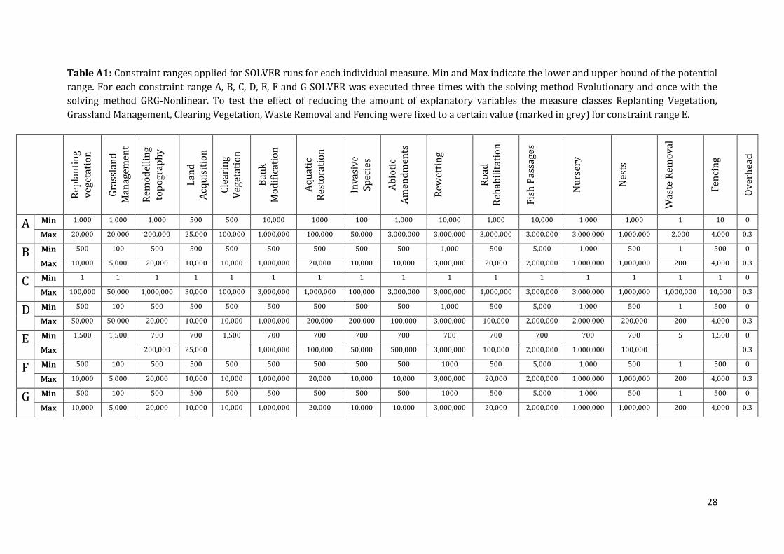
Table A1: Constraint ranges applied for SOLVER runs for each individual measure. Min and Max indicate the lower and upper bound of the potential

range. For each constraint range A, B, C, D, E, F and G SOLVER was executed three times with the solving method Evolutionary and once with the

solving method GRG-Nonlinear. To test the effect of reducing the amount of explanatory variables the measure classes Replanting Vegetation,

Grassland Management, Clearing Vegetation, Waste Removal and Fencing were fixed to a certain value (marked in grey) for constraint range E.

Rep

lan

tin

g ve

geta

tio

n

Gra

ssla

nd

M

anag

emen

t

Rem

od

elli

ng

top

ogr

aph

y

Lan

d

Acq

uis

itio

n

Cle

arin

g V

eget

atio

n

Ban

k

Mo

dif

icat

ion

Aq

uat

ic

Res

tora

tio

n

Inva

sive

Sp

ecie

s

Ab

ioti

c A

men

dm

ents

Rew

etti

ng

Ro

ad

Reh

abil

itat

ion

Fis

h P

assa

ges

Nu

rser

y

Nes

ts

Was

te R

emo

val

Fen

cin

g

Ove

rhea

d

A Min 1,000 1,000 1,000 500 500 10,000 1000 100 1,000 10,000 1,000 10,000 1,000 1,000 1 10 0

Max 20,000 20,000 200,000 25,000 100,000 1,000,000 100,000 50,000 3,000,000 3,000,000 3,000,000 3,000,000 3,000,000 1,000,000 2,000 4,000 0.3

B Min 500 100 500 500 500 500 500 500 500 1,000 500 5,000 1,000 500 1 500 0

Max 10,000 5,000 20,000 10,000 10,000 1,000,000 20,000 10,000 10,000 3,000,000 20,000 2,000,000 1,000,000 1,000,000 200 4,000 0.3

C Min 1 1 1 1 1 1 1 1 1 1 1 1 1 1 1 1 0

Max 100,000 50,000 1,000,000 30,000 100,000 3,000,000 1,000,000 100,000 3,000,000 3,000,000 1,000,000 3,000,000 3,000,000 1,000,000 1,000,000 10,000 0.3

D Min 500 100 500 500 500 500 500 500 500 1,000 500 5,000 1,000 500 1 500 0

Max 50,000 50,000 20,000 10,000 10,000 1,000,000 200,000 200,000 100,000 3,000,000 100,000 2,000,000 2,000,000 200,000 200 4,000 0.3

E Min 1,500 1,500 700 700 1,500 700 700 700 700 700 700 700 700 700 5 1,500 0

Max 200,000 25,000 1,000,000 100,000 50,000 500,000 3,000,000 100,000 2,000,000 1,000,000 100,000 0.3

F Min 500 100 500 500 500 500 500 500 500 1000 500 5,000 1,000 500 1 500 0

Max 10,000 5,000 20,000 10,000 10,000 1,000,000 20,000 10,000 10,000 3,000,000 20,000 2,000,000 1,000,000 1,000,000 200 4,000 0.3

G Min 500 100 500 500 500 500 500 500 500 1000 500 5,000 1,000 500 1 500 0

Max 10,000 5,000 20,000 10,000 10,000 1,000,000 20,000 10,000 10,000 3,000,000 20,000 2,000,000 1,000,000 1,000,000 200 4,000 0.3

29

Table A2: Harmonized Indices of Consumer Prices (HICP) taken from Eurostat (last update: May 16 2013)

GEO/TIME 1996 1997 1998 1999 2000 2001 2002 2003 2004 2005 2006 2007 2008 2009 2010 2011 2012

Belgium 85.25 86.53 87.32 88.31 90.67 92.88 94.32 95.75 97.53 100 102.33 104.19 108.87 108.86 111.40 115.14 118.16

Bulgaria : 56.90 67.53 69.27 76.41 82.04 86.80 88.84 94.30 100 107.42 115.55 129.36 132.56 136.58 141.21 144.58

Czech Republic 72.2 78.0 85.6 87.1 90.6 94.7 96.1 96.0 98.4 100 102.1 105.1 111.7 112.4 113.7 116.2 120.3

Denmark 84.3 85.9 87.0 88.8 91.2 93.3 95.6 97.5 98.3 100 101.8 103.5 107.3 108.4 110.8 113.8 116.5

Germany 88.6 90.0 90.5 91.1 92.4 94.1 95.4 96.4 98.1 100 101.8 104.1 107.0 107.2 108.4 111.1 113.5

Estonia 65.97 72.09 78.42 80.85 84.03 88.76 91.95 93.22 96.05 100 104.45 111.49 123.31 123.56 126.95 133.40 139.02

Ireland 75.7 76.7 78.3 80.3 84.5 87.8 92.0 95.7 97.9 100 102.7 105.6 108.9 107.1 105.4 106.6 108.7

Greece 72.68 76.63 80.10 81.81 84.18 87.26 90.67 93.79 96.63 100 103.31 106.40 110.90 112.40 117.68 121.35 122.61

Spain 77.92 79.39 80.79 82.59 85.47 87.88 91.04 93.86 96.73 100 103.56 106.51 110.91 110.64 112.90 116.35 119.18

France 86.64 87.75 88.34 88.84 90.46 92.07 93.86 95.89 98.14 100 101.91 103.55 106.82 106.93 108.79 111.28 113.75

Italy 81.8 83.3 85.0 86.4 88.6 90.7 93.1 95.7 97.8 100 102.2 104.3 108.0 108.8 110.6 113.8 117.5

Cyprus 78.70 81.31 83.21 84.15 88.25 90.00 92.51 96.18 98.00 100 102.25 104.46 109.03 109.22 112.02 115.93 119.52

Latvia 69.31 74.89 78.11 79.77 81.87 83.94 85.58 88.10 93.55 100 106.57 117.32 135.21 139.62 137.91 143.73 147.02

Lithuania 80.15 88.39 93.15 94.51 95.53 97.01 97.34 96.29 97.41 100 103.79 109.83 122.01 127.09 128.60 133.90 138.14

Luxembourg 81.18 82.30 83.10 83.94 87.12 89.21 91.04 93.36 96.37 100 102.96 105.69 110.01 110.02 113.10 117.32 120.72

Hungary 46.04 54.53 62.28 68.49 75.31 82.15 86.46 90.50 96.63 100 104.03 112.28 119.05 123.85 129.70 134.79 142.42

Malta 77.97 81.02 84.02 85.94 88.55 90.77 93.14 94.95 97.53 100 102.58 103.29 108.13 110.12 112.37 115.19 118.91

Netherlands 80.43 81.92 83.38 85.07 87.06 91.51 95.05 97.18 98.52 100 101.65 103.26 105.54 106.57 107.56 110.23 113.34

Austria 87.21 88.22 88.95 89.41 91.16 93.25 94.83 96.06 97.94 100 101.69 103.93 107.28 107.71 109.53 113.42 116.34

Poland 57.6 66.3 74.1 79.4 87.4 92.0 93.8 94.5 97.9 100 101.3 103.9 108.3 112.6 115.6 120.1 124.5

Portugal 78.12 79.60 81.36 83.13 85.46 89.23 92.51 95.52 97.92 100 103.04 105.54 108.34 107.36 108.85 112.72 115.85

Romania 5.01 12.77 20.31 29.62 43.15 58.02 71.09 81.94 91.68 100 106.60 111.84 120.69 127.43 135.17 143.04 147.88

Slovenia 56.50 61.21 66.05 70.09 76.36 82.90 89.09 94.16 97.60 100 102.54 106.39 112.28 113.25 115.62 118.03 121.35

Slovakia 53.71 56.93 60.74 67.09 75.27 80.66 83.48 90.52 97.28 100 104.26 106.23 110.41 111.43 112.21 116.79 121.16

Finland 87.30 88.37 89.56 90.73 93.41 95.90 97.82 99.10 99.24 100 101.28 102.88 106.91 108.66 110.49 114.16 117.77

Sweden 87.51 89.09 90.01 90.51 91.67 94.12 95.94 98.18 99.18 100 101.50 103.20 106.65 108.72 110.80 112.31 113.36

United Kingdom 88.1 89.7 91.1 92.3 93.1 94.2 95.4 96.7 98.0 100 102.3 104.7 108.5 110.8 114.5 119.6 123.0

30

Table A3: Price Level Index (PLI) data used in the report (based on Eurostat).

GEO/TIME 1995 1996 1997 1998 1999 2000 2001 2002 2003 2004 2005 2006 2007 2008 2009 2010 2011

Belgium 113.8 110.5 106.2 107.3 106.5 102.5 103.2 101.3 104.0 106.4 107.5 108.4 109.2 111.7 114.0 112.2 112.8

Bulgaria 25.6 21.6 25.9 30.2 30.9 31.8 33.4 33.4 33.9 35.1 36.6 38.1 40.1 42.7 44.7 44.7 45.2

Czech Republic 38.1 41.0 41.4 45.0 44.3 45.9 48.6 54.4 52.2 53.2 57.4 60.8 61.8 73.1 69.8 73.1 73.6

Denmark 137.9 135.4 131.8 130.7 131.7 129.8 132.4 130.8 136.0 134.1 137.7 137.1 136.1 137.4 139.7 136.3 137.3

Germany 125.2 120.0 115.3 114.6 112.7 111.2 111.3 110.3 108.6 106.4 103.5 102.9 102.3 103.8 107.5 105.3 104.6

Estonia 37.9 44.7 46.7 49.8 51.3 52.4 55.6 55.9 56.9 57.7 60.0 63.9 68.3 70.2 69.7 69.1 70.4

Ireland 94.8 96.9 105.2 103.2 107.5 110.7 115.7 117.5 120.1 119.4 120.7 120.9 118.0 121.7 118.5 110.7 108.9

Greece 76.9 79.6 81.2 79.7 82.3 78.9 78.2 77.3 81.5 82.6 85.3 85.9 88.5 89.7 92.7 92.6 92.9

Spain 86.4 87.7 84.4 83.6 84.7 84.5 86.2 85.9 89.1 90.1 91.4 90.3 89.7 92.1 94.2 93.6 93.4

France 119.1 117.9 113.1 112.2 111.0 108.0 107.0 105.9 111.0 111.6 110.3 110.9 110.0 112.8 114.4 112.8 112.7

Italy 85.5 94.4 95.9 94.1 94.6 94.0 94.1 99.0 101.1 103.6 103.5 102.4 100.6 100.9 103.5 103.8 103.6

Cyprus 84.0 83.1 84.1 85.4 85.8 85.9 85.7 86.1 88.5 88.0 88.2 88.6 88.0 87.6 88.8 88.8 89.0

Latvia 33.3 36.6 40.4 41.4 44.5 51.2 51.7 50.3 47.8 48.9 51.8 57.5 66.6 71.9 68.2 65.4 66.9

Lithuania 27.2 32.6 39.9 41.3 42.1 47.2 47.6 48.1 47.0 48.4 51.4 54.1 57.4 62.9 61.9 59.7 61.4

Luxembourg 118.4 114.7 111.6 110.0 108.9 108.1 110.5 109.4 111.5 109.5 113.8 112.3 113.9 115.9 120.5 120.6 120.6

Hungary 44.7 44.6 47.0 45.7 46.2 47.7 50.2 55.4 56.3 59.6 61.9 59.7 64.3 65.8 59.5 60.8 60.7

Malta 57.6 62.4 64.2 64.7 65.5 68.0 71.1 69.7 68.4 67.4 67.7 69.0 69.9 71.7 72.7 72.1 72.8

Netherlands 114.6 110.5 106.1 105.1 104.9 102.7 105.6 105.6 109.7 107.9 107.0 106.6 105.6 107.7 111.8 110.4 109.7

Austria 116.3 112.4 107.6 106.4 106.0 103.6 106.9 104.9 104.7 103.8 105.9 105.2 106.8 109.0 112.1 109.7 110.2

Poland 44.3 46.9 47.8 49.5 47.6 52.8 59.0 55.5 49.5 48.8 55.5 58.1 60.0 67.6 57.2 60.2 59.3

Portugal 79.1 79.8 79.4 80.5 80.6 80.5 82.2 82.9 83.6 85.0 81.7 81.3 81.3 83.0 84.1 82.6 82.4

Romania 26.5 25.3 29.4 36.4 32.2 36.5 36.8 37.1 37.3 38.1 46.9 49.9 55.8 55.5 49.6 50.8 52.0

Slovenia 73.7 71.5 71.5 73.0 72.8 70.9 72.4 73.1 74.6 72.7 73.1 74.7 77.5 81.1 85.6 84.7 83.9

Slovakia 40.1 40.5 42.1 41.9 39.5 42.8 42.3 43.6 47.7 51.2 52.8 55.2 59.9 65.7 67.9 67.9 69.1

Finland 124.2 120.8 118.0 116.4 116.0 114.5 117.9 117.5 119.6 115.8 116.7 116.7 115.8 117.4 120.0 120.1 122.1

Sweden 119.7 128.2 125.8 122.8 122.0 124.4 117.7 119.5 121.1 118.5 120.7 120.5 118.3 116.7 111.5 123.4 128.8

United Kingdom 92.2 93.0 107.3 111.4 114.6 120.0 117.4 116.8 109.6 110.7 111.1 112.9 116.1 104.5 97.8 101.0 101.8

Europe Direct is a service to help you find answers to your questions about the European Union

Freephone number (*): 00 800 6 7 8 9 10 11

(*) Certain mobile telephone operators do not allow access to 00 800 numbers or these calls may be billed.

A great deal of additional information on the European Union is available on the Internet.

It can be accessed through the Europa server http://europa.eu.

How to obtain EU publications

Our publications are available from EU Bookshop (http://bookshop.europa.eu),

where you can place an order with the sales agent of your choice.

The Publications Office has a worldwide network of sales agents.

You can obtain their contact details by sending a fax to (352) 29 29-42758.

European Commission

EUR 27494 EN – Joint Research Centre – Institute for Environment and Sustainability

Title: Costs of restoration measures in the EU based on an assessment of LIFE projects

Authors: Andreas Dietzel, Joachim Maes

Luxembourg: Publications Office of the European Union

2015 – 30 pp. – 21.0 x 29.7 cm

EUR – Scientific and Technical Research series – ISSN 1831-9424 (online)

ISBN 978-92-79-52208-6 (PDF)

doi:10.2788/235713

ISBN 978-92-79-52208-6

doi:10.2788/235713

JRC Mission As the Commission’s in-house science service, the Joint Research Centre’s mission is to provide EU policies with independent, evidence-based scientific and technical support throughout the whole policy cycle. Working in close cooperation with policy Directorates-General, the JRC addresses key societal challenges while stimulating innovation through developing new methods, tools and standards, and sharing its know-how with the Member States, the scientific community and international partners.

Serving society Stimulating innovation Supporting legislation

LB

-NA

-27

49

4-E

N-N