Cost optimization of the preliminary design layout of ...
299
University of Wollongong Research Online University of Wollongong esis Collection University of Wollongong esis Collections 2013 Cost optimization of the preliminary design layout of reinforced concrete framed buildings Pezhman Sharafi University of Wollongong, psharafi@uow.edu.au Research Online is the open access institutional repository for the University of Wollongong. For further information contact the UOW Library: [email protected] Recommended Citation Sharafi, Pezhman, Cost optimization of the preliminary design layout of reinforced concrete framed buildings, Doctor of Philosophy thesis, School of Civil, Mining and Environmental Engineering, University of Wollongong, 2013. hp://ro.uow.edu.au/theses/3916
Transcript of Cost optimization of the preliminary design layout of ...
University of WollongongResearch Online
University of Wollongong Thesis Collection University of Wollongong Thesis Collections
2013
Cost optimization of the preliminary design layoutof reinforced concrete framed buildingsPezhman SharafiUniversity of Wollongong, [email protected]
Research Online is the open access institutional repository for theUniversity of Wollongong. For further information contact the UOWLibrary: [email protected]
Recommended CitationSharafi, Pezhman, Cost optimization of the preliminary design layout of reinforced concrete framed buildings, Doctor of Philosophythesis, School of Civil, Mining and Environmental Engineering, University of Wollongong, 2013. http://ro.uow.edu.au/theses/3916
School of Civil, Mining and Environmental Engineering
Cost Optimization of the Preliminary Design Layout of
Reinforced Concrete Framed Buildings
By
Pezhman Sharafi
This thesis is submitted in fulfilment of the award of the Degree
DOCTOR OF PHILOSOPHY
(Civil Engineering)
University of Wollongong
June 2013
i
ABSTRACT
This thesis proposes an explicit methodology for optimising the cost of the
preliminary design layout of framed Reinforced Concrete (RC) buildings. The design
of the column layout for RC buildings was studied first, followed by the optimum
location of columns for the RC structures. The next step was to optimise the layout
including the location of the columns and the rectilinear shapes for the plan layout
and the rectilinear shapes proposed for the RC buildings.
In order to formulate such a methodology a model was developed to represent the
mathematical relationship between the costs of concrete, longitudinal steel, shear
steel, and formwork, and the number and size of the spans and the shape of the plan.
Such a model illustrates how variations in the layout affects the cost elements, and
how each cost element varies when the layout changes.
A unique mathematical relationship between the design layout and cost elements was
formulated for structural systems such as continuous beams, plane frames, 3D
frames, flat plates and beam-slab floor systems, in order to study different responses
towards variations in the layout. This is a novel approach that can easily be used to
optimise the design of various types of large RC structures and also account for
constraints imposed by the design standards.
This approach makes use of cross sectional effects such as the positive and negative
bending moments, and the shear and axial forces along the structural members for
each structural system to derive a novel cost function as an alternative to traditional
cost functions for optimising the layout of RC structures where design variables are
used. These novel functions can be used to optimise the cost and layout of RC
ii
structures, because they are represented in a new space that takes the cost elements
and layout design variables into account.
A combined approach was adapted to deal with a new structural optimisation
problem, so an automated technique for optimising the preliminary layout of framed
buildings with rectilinear patterns is presented. This method supports all types of
rectilinear buildings (also known as orthogonal or iso-oriented) plans, including
rectangular frames where the number and size of the spans and the shape of the plan
can be variables. To that end, the knapsack problem was used as a basic applied
combinatorial optimisation problem.
Ant Colony Optimization (ACO), as a robust metaheuristic, was used to solve the
combinatorial optimisation arising from the structural optimisation problem.
Numerical examples for each structural system are presented to demonstrate the
robustness and practicality of the methodology and algorithms.

iii
ACKNOWLEDGEMENTS
I wish to express my profound gratitude to my supervisors, A/Prof. Muhammad Hadi
and Dr. Lip Teh at the University of Wollongong, Wollongong, Australia for their
invaluable advice and guidance during my PhD studies. Their constant support and
encouragement are gratefully acknowledged.
I would also like to thank the School of Civil, Mining and Environmental
Engineering, University of Wollongong (UOW), for providing all the necessary
facilities and working conditions for my research. I am also grateful to UOW for the
APA scholarship which enabled me to undertake the PhD program.
Finally, I would like to express my deepest gratitude to my family, whose constant
love and prayer became an active strength during the completion of this research, and
to my friends for their understandings and patience during my study at the University
of Wollongong.
iv
LIST OF PUBLICATIONS
Book Chapters:
Sharafi, P., Hadi, M. N. S. and Teh, L. H. (2013), "Cost Optimization of Column Layout Design of
Reinforced Concrete Buildings", Metaheuristics and Applications in Civil Engineering, Book
chapter. Elsevier, London.
Journal Papers:
Sharafi, P., Hadi, M. N. S. and Teh, L. H. (2012). "Heuristic Approach for Optimum Cost and
Layout Design of 3D Reinforced Concrete Frames", ASCE journal of structural engineering,
Vol.138(7), 853-863,
Sharafi, P., Hadi, M. N. S. and Teh, L. H. (2012), "Geometric Design Optimization or Dynamic
Response Problem of Continuous Reinforced Concrete Beams" Accepted for publishing by ASCE
Journal of computing in civil engineering. doi: 10.1061/(ASCE)CP.1943-5487.0000263
Sharafi, P.,Teh, L. H and Hadi, M. N. S. (2013), "Graph theory in shape optimization of thin-
walled sections", submitted to the journal of Engineering Structures.
Sharafi, P., Hadi, M. N. S. and Teh, L. H. (2013), "Optimum Preliminary layout design of frames
of orthogonal patterns: A Knapsack approach", Submitted to the ASCE journal of Structural
Engineering.
Sharafi, P., Hadi, M. N. S. and Teh, L. H. (2013), "Optimum Preliminary layout design of frames
of orthogonal patterns: Algorithm and Applications", Submitted to the ASCE journal of Structural
Engineering.
Conference Proceedings:
Sharafi, P., Hadi, M. N. S. and Teh, L. H. (2012), "Optimum Column Layout Design of Reinforced
Concrete Frames under Wind Loading", TOPICS ON THE DYNAMICS OF CIVIL
STRUCTURES, VOLUME 1 Conference Proceedings of the Society for Experimental Mechanics
Series, Volume 26, 327-340,
Sharafi, P., Hadi, M. N. S. and Teh, L. H. (2012), "Optimum Spans' Lengths of Multi-Span
Reinforced Concrete Beams under Dynamic Loading", TOPICS ON THE DYNAMICS OF CIVIL
STRUCTURES, VOLUME 41 Conference Proceedings of the Society for Experimental
Mechanics Series, Volume 26, 353-361
Sharafi, P., Hadi, M. N. S. and Teh, L. H. (2012), "A Novel Formulation for the Geometric Layout
and Cost Optimization of Flat Slab Floor Systems ", The proceedings of the Australasian Structural
Engineering Conference, ASEC 2012
v
Sharafi, P., Hadi, M. N. S. and Teh, L. H. (2013), "A Methodology for Cost Optimization of the
Layout Design of Multi-Span Reinforced Concrete Beams" Accepted for CIVIL COMP 30st.
Sharafi, P., Hadi, M. N. S. and Teh, L. H. (2013), "A Novel Combinatorics Approach for Optimum
Conceptual Design of Buildings of Orthogonal Shapes", Accepted for CIVIL COMP 30st, 2013.
Sharafi, P., Hadi, M. N. S. and Teh, L. H. (2013), "Theory Based Sensitivity Analysis and Damage
Detection of Steel Roof Sheeting for Hailstone Impact", TOPICS ON THE DYNAMICS OF
CIVIL STRUCTURES, VOLUME 4, Conference Proceedings of the Society for Experimental
Mechanics Series, VOLUME 4, 243-252
Sharafi, P., Hadi, M. N. S. and Teh, L. H. (2013), "Sizing Optimization of Trapezoidal Corrugated
Roof Sheeting Supporting Solar Panels under Wind Loading", TOPICS ON THE DYNAMICS OF
CIVIL STRUCTURES, VOLUME 4, Conference Proceedings of the Society for Experimental
Mechanics Series, VOLUME 4, 535-542
vi
TABLE OF CONTENTS
ABSTRACT .................................................................................................................. i
ACKNOWLEDGEMENTS ........................................................................................ iii
LIST OF PUBLICATIONS ........................................................................................ iv
TABLE OF CONTENTS ............................................................................................ vi
LIST OF FIGURES .................................................................................................... ix
1 Introduction ............................................................................................................... 1
1.1 Background of the study .............................................................................. 1
1.2 Structural optimisation ................................................................................. 3
1.2.1 Theoretical background ............................................................................ 8
1.2.2 The topology and geometric layout optimisation of structures ................ 9
1.2.3 Optimisation techniques and terminology ............................................. 16
1.3 Research objectives and Scope .................................................................. 17
1.4 Research methodology ............................................................................... 20
1.5 Chapter Outline .......................................................................................... 22
2 Optimising the Cost of Reinforced Concerete Structures ....................................... 23
2.1 Introduction ................................................................................................ 23
2.2 Optimising the Cost of Structures .............................................................. 24
2.3 Multi-Objective Optimisation of Structures .............................................. 27
2.4 Optimising the Cost and Layout ................................................................ 29
2.5 Summary .................................................................................................... 33
3 Combinatorial Optimisation Techniques ................................................................ 35
3.1 Introduction ................................................................................................ 35
3.2 Combinatorial Optimisation Problems ....................................................... 36
3.3 Graph theory: Basic Terminology .............................................................. 39
3.4 Shortest Path Problems .............................................................................. 40
3.4.1 Shortest Path Problem for Column Layout Design ................................ 42
3.5 Knapsack Problems .................................................................................... 45
3.5.1 Knapsack Problems for Plan Layout Design ......................................... 48
3.6 Randomised Search Heuristics and Methaheuristics ................................. 60
3.7 Ant Colony Optimisation ........................................................................... 67
3.7.1 ACO for Multi-objective Optimisation .................................................. 74
3.8 Summary .................................................................................................... 77
vii
4 Optimum Column Layout Design for Continuous Beams ...................................... 80
4.1 Introduction ................................................................................................ 80
4.2 Optimum Design for Static Loading .......................................................... 81
4.2.1 Mathematical formulation ...................................................................... 86
4.2.2 Optimisation Problem formulation ........................................................ 91
4.2.3 ACO Algorithm ...................................................................................... 94
4.2.4 Numerical Examples ............................................................................ 100
4.3 Optimum Design for Dynamic Loading .................................................. 104
4.3.1 Mathematical Formulation ................................................................... 108
4.3.2 Optimisation Problem Formulation ..................................................... 110
4.3.3 ACO Algorithm .................................................................................... 113
4.3.4 Numerical Examples ............................................................................ 116
4.4 Summary .................................................................................................. 123
5 Optimum Column Layout Design of Plane Frames under Wind Loading............ 125
5.1 Introduction .............................................................................................. 125
5.2 Mathematical formulation ........................................................................ 128
5.3 Optimisation Problem formulation .......................................................... 139
5.4 ACO algorithm ......................................................................................... 141
5.5 Numerical example .................................................................................. 146
5.6 Summary .................................................................................................. 149
6 Optimum Layout Design of RC Buildings with Rectangular Plan ....................... 150
6.1 Introduction .............................................................................................. 150
6.2 Mathematical formulation ........................................................................ 154
6.3 Optimisation Problem formulation .......................................................... 158
6.4 ACO algorithm ......................................................................................... 159
6.5 Numerical examples ................................................................................. 165
6.6 Summary .................................................................................................. 170
7 Optimum Layout Design of Rectangular Flat Plate Floor Systems ...................... 171
7.1 Introduction .............................................................................................. 171
7.2 Mathematical formulation ........................................................................ 175
7.3 Optimization Problem formulation .......................................................... 183
7.4 ACO algorithm ......................................................................................... 187
7.5 Numerical examples ................................................................................. 191
viii
7.6 Summary .................................................................................................. 195
8 Optimum Layout Design for RC Beam-Slab Floor systems ................................. 197
8.1 Introduction .............................................................................................. 197
8.2 Mathematical formulation ........................................................................ 200
8.3 Optimisation Problem formulation .......................................................... 209
8.4 ACO algorithm ......................................................................................... 211
8.5 Numerical examples ................................................................................. 218
8.6 Summary .................................................................................................. 224
9 Optimum Layout Design of Rectilinear RC Buildings ........................................ 226
9.1 Introduction .............................................................................................. 226
9.2 Statement of the problem ......................................................................... 229
9.3 Optimisation Problem Formulation ......................................................... 232
9.3.1 Formulation for Cost ............................................................................ 234
9.3.2 Formulation for Plan Regularity .......................................................... 239
9.3.3 Combinatorial Optimisation Formulation ............................................ 240
9.4 Multi-Objective Problem ......................................................................... 243
9.5 ACO Algorithm ........................................................................................ 245
9.6 Numerical Example .................................................................................. 254
9.7 Summary .................................................................................................. 258
10 Conclusion .......................................................................................................... 261
References ........................................................................................................... 266
ix
LIST OF FIGURES
Figure 3-1 A path and a cycle on directed graphs .................................................................. 40
Figure 3-2. Directed graph model for 2D frames ................................................................... 43
Figure 3-3. Directed graph model for 3D frames ................................................................... 44
Figure 3-4. Representing the building's layout plan by an arrangement of rectangles .......... 48
Figure 3-5. A framed building of rectilinear layout plan ....................................................... 49
Figure 3-6. Levels and spans in the layout plan ..................................................................... 51
Figure 3-7. The multiple knapsack model for layout optimization ........................................ 53
Figure 3-8. The knapsack model for special case 1 ............................................................... 56
Figure 3-9. The knapsack model for special case 2 ............................................................... 57
Figure 3-10. The knapsack model for special case 3 ............................................................. 59
Figure 3-11. The Procedure ACO Algorithm ........................................................................ 69
Figure 3-12. The Algorithmic Skeleton for Multi-objective ACO ........................................ 75
Figure 4-1. An arbitrary section of a rectangular RC beam ................................................... 87
Figure 4-2. A multi-span rectangular RC beam under arbitrary static loading ...................... 91
Figure 4-3. Constructing a graph for the Ant algorithm ........................................................ 94
Figure 4-4. The ACO Flowchart ............................................................................................ 96
Figure 4-5. Example 1: Three-span beam with uniformly distributed loads ....................... 101
Figure 4-6. Typical convergence history for the presented ACO algorithm for Example 1 102
Figure 4-7. Example 2 - A five span beam and selected sections to control the cost .......... 103
Figure 4-8. Typical convergence history for the presented ACO algorithm for Example 2 103
Figure 4-9. A multi-span rectangular RC beam ................................................................... 107
Figure 4-10. Construction Graph for the ACO Algorithm ................................................... 115
Figure 4-11. Numerical Example: An M-Span Continuous RC Beam ................................ 117
Figure 4-12. A multi-span beam and the coresponding construction graph the algorithm .. 118
Figure 4-13. Example: a five span beam and selected sections to control the cost ............. 122
Figure 4-14. Typical convergence history for the presented ACO algorithm ..................... 123
Figure 5-1. Cross-sectional parameters for a column .......................................................... 134
Figure 5-2. The construction graph for a plane frame ......................................................... 143
Figure 5-3. Numerical Example: An eight story building.................................................... 147
Figure 5-4. Typical convergence history for the presented ACO algorithm ....................... 149
Figure 6-1. The Construction graph for the ACO algorithm ............................................... 161
Figure 6-2. Plane view of the primary design of the 3D frames .......................................... 167
Figure 6-3. Typical convergence history for the ACO algorithm ........................................ 169
Figure 7-1. A typical flat plate floor system ........................................................................ 172
x
Figure 7-2. Equivalent frame strips for flat plates ............................................................... 176
Figure 7-3. A typical flat plate system plan for Example 1 and 2........................................ 192
Figure 7-4. Typical convergence history for the ACO algorithm for Example 1 ................ 194
Figure 7-5. Typical convergence history for the ACO algorithm for Example ................... 195
Figure 8-1. A typical Beam-Slab floor system .................................................................... 198
Figure 8-2. Spans and Control Sections in the x and y directions of slabs ......................... 201
Figure 8-3. A General Beam Cross-Section and the Related Parameters ........................... 204
Figure 8-4. A General Column Cross-section and the Related Parameters ........................ 207
Figure 8-5. Example 1: A four storey RC building ............................................................. 219
Figure 8-6. Convergence history for the ACO algorithm. .................................................. 224
Figure 9-1. A multi-storey building with a rectilinear frame ............................................... 236
Figure 9-2. The construction Sub-Graph for the First knapsack .......................................... 250
Figure 9-3. The construction Sub-Graph for the Knapsack 2 through m ............................. 251
Figure 9-4. Numerical Example ........................................................................................... 255
Figure 9-5. Numerical Example: Initial plan design and the corresponding Knapsacks ..... 256
Figure 9-6. Numerical Example: Schematic results for 𝜆=0.5 ............................................. 257
Figure 9-7. Numerical Example: Schematic results for 𝜆=0.8 ............................................. 258
Figure 9-8. Numerical Example: Schematic results for 𝜆=0.2 ............................................ 258
LIST OF TABLES
Table 4-1. Results for Different Number of Spans .............................................................. 120
Table 9-1. Parameters for ACO Algorithm ......................................................................... 257
1
1 Introduction
1.1 Background of the study
The structural design process may be divided into four stages: formulating the
functional requirements, conceptual design, optimisation, and detailing. An iterative
procedure is often required for each stage before the final solution is achieved; a
process that is usually carried out without considering the relative costs of concrete,
steel, formwork, or other relevant costs. In an optimal design the structural behaviour,
design loads and geometrical constraints are specified and then the cost or the
objective function is defined. The aim of this computational effort is to determine the
geometry to achieve the desired behaviour at the lowest possible cost. It is important
to be familiar with the concepts explained in this section in order to understand the
nuances of this research.
In designing buildings, achieving a planned layout is one of the primary objectives
because the preliminary layout of a structure impacts on the entire design process and,
the total costs, although preliminary design layouts of buildings are often performed
based only on the architectural requirements. In the preliminary design phase the
architects may have the liberty to choose from a number of different layout plans that
meet the architectural requirements, in which case there is a need for a criterion or
2
criteria that helps the designer choose the most economic one. In order to select the
most economical plan among the various layouts that satisfy the architectural
requirements, one needs to first establish the reciprocal effects of cost factors and
layout variables. That is, achieving an economical layout plan requires a simultaneous
consideration of both cost and layout elements. Combining a robust optimisation
algorithm with a proper structural analysis, and a design method that incorporates the
relevant costs will lead to a powerful system for optimising structural design. In such a
comprehensive process, selecting an appropriate preliminary geometric design layout
of structures is important because it influences all the subsequent stages of the design
procedure.
In fact, for this new methodology to be widely applicable the traditional cost design
space must be shifted to a new one in order to establish a comprehensive approach that
represents the cost factors and layout design variables. The traditional cost variables
used for more than four decades to optimise the cost of structures are best suited for
structures with a predefined layout design but are impractical for optimising the cost
of multi-member structures. By shifting to a new design space the cost functions
proposed as a part of this methodology simplifies optimising the cost of the layout
design of reinforced concrete structures, and is applicable for a multi-variable
optimisation of reinforced concrete structures such as the cost and layout optimisation
problem.
Preliminary (conceptual) design is the earliest phase of the design process and
commences with a set of initial concepts. Designers at this early stage must understand
the many factors affecting the project being designed, such as its efficiency,
construction costs, operating costs, the quality and comfort of the built project, and the
potential for generating revenue. Significant complexity comes from the need to

3
determine the relative benefits of all of these various quantities and qualities (Rush
1986). The decision for the geometric layout design of a structure, say the column
layout of a building, is made in the preliminary phase, but such a decision affects the
whole design process and relevant costs. In order to optimise the cost in a layout
design problem, the designer may face various variables during this process. The
process of simultaneously optimising two or more conflicting objectives subject to
certain constraints is called multi-criteria or multi-objective optimisation.
This thesis is about defining the problem of t optimising the cost of the design layout
of framed Reinforced Concrete (RC) structures and seeking a methodology for
considering the cost components in the preliminary layout optimisation process.
1.2 Structural optimisation
Optimal structural design is becoming increasingly significant due to limited material
resources, and its environmental impact and technological competition, all of which
demand high performance, light weight and more importantly, low life-cycle-cost
structures. The design of a safe and economical structure is one of the main concerns
of structural engineers. Economy in design can be achieved through an optimisation
procedure by aiming to find the most efficient structure that will satisfy the chosen
criteria. Combining an optimisation procedure with structural modelling, and analysis
and design methods, and then augmenting them with the cost of systems and materials
in a unique process will lead to the development of a powerful optimisation system.
The increasing demand on engineers to lower production costs to withstand global
competition has prompted them to look for rigorous methods of decision making, such
4
as optimisation methods, to design and produce products and systems both
economically and efficiently. Optimisation techniques, having reached a degree of
maturity in recent years, are being used in a wide spectrum of industries, including
aerospace, automotive, chemical, electrical, construction, and manufacturing industries
(Rao 2009a). With rapidly advancing computer technology, computers are becoming
more powerful, and correspondingly, the size and complexity of problems that can be
solved using optimisation techniques is increasing. Optimisation methods, coupled
with the modern tools of computer aided design, are also being used to enhance the
creative process of preliminary (conceptual) and detailed design of engineering
systems.
Contemporary structural optimisation has its roots in the 1960s with Lucien Schmidt‘s
seminal paper. While the 1960s and 1970s were characterised by difficulties in solving
even small optimisation problems (forgetting for the moment the optimal criteria
methods), the 1990s were characterised by discussions regarding the use of
mathematical programming methods for solving large systems (Spillers and MacBain
2009).
Since the 1960s a significant amount of research has been published in the area of
structural optimisation, with the vast majority of these papers dealing with minimising
the weight of a structure. While the weight of a structure constitutes a significant part
of the cost, a minimum weight design is not necessarily the minimum cost of a design.
Only a small fraction of the papers published on structural optimisation deal with the
cost optimisation problem, most of them deal with structural elements such as beams,
although some journal papers have been published on the cost optimisation of realistic
three-dimensional structures. As such, there is a need to perform research on the cost
optimisation of realistic three-dimensional structures, especially large structures with
5
hundreds of members where optimisation can result in substantial savings. The results
of such research efforts will be of great value to practicing engineers.
This section gives an overview of the related literature, focusing mainly on the cost
optimisation of structures, layout optimisation, and the methods used in structural
optimisation to show that this thesis is an original work albeit closely related to other
research fields.
Over the past decades, considerable progress has been achieved in the optimum design
of structures via mathematical programming methods such as the Lagrangian
multipliers method, convex programming, linear programming, and sequential
unconstrained minimisation techniques and evolutionary algorithms.
Unlike steel structures where optimization is the problem of minimising weight, the
optimisation of reinforced concrete structures must be formulated as a cost
minimisation problem because different materials are involved. Only a small fraction
of the hundreds of papers published on the optimisation of steel structures deals with
optimising costs (Adeli & Sarma 2006); while minimising the weight does not
necessarily lead to the minimum cost and in reality, a minimum weight design may not
be a minimum cost design. Apart from the cost of materials, many other factors
influence the total construction cost of a structure.
Up to the late 1990s, few research studies had reported on the optimisation of the
overall cost of a three-dimensional steel structure subject to the constraints of
commonly used design standards. While for the structural optimisation methodology
in general and the cost optimisation approach in particular, to be embraced by the
structural engineering community, the focus of future research should be on large
6
structures subjected to the actual constraints of commonly used design codes rather
than single members subjected to non-realistic constraints (Burns 2002).
The computerised analysis of structures via models that discretise the structure into a
large number of pieces known as finite elements, has become prevalent in the 1960s,
numerical optimisation based on finite element models was started in the early 1960s
by L. Schmit and his students. Significant research studies on the practical optimum
design of structures based on cost minimisation goes back to the early 1970s (Adeli &
Sarma 2006), years that were characterised by applications for civil engineering truss
structures where the design variables were cross sectional areas of the elements. Later
these variables were generalised to cross sectional dimensions of beams and
thicknesses of plates. This class of design variables, the so called sizing variables, are
distinct in that optimisation can be carried out with only superficial changes in the
finite element model (Floudas & Pardalos 2009).
Historically there has been a tension between proponents of classical optimisation
methods who claimed that the users of optimality criteria methods were lacking in
theory, and the users of heuristic schemes such as optimality criteria methods who at
the same time claimed that the classical methods were incapable of solving real (large)
structures. In view of the tools now available to the engineer, these arguments can
diminish in importance although the optimality criteria methods still have enormous
physical appeal (Spillers & MacBain 2009).
In the structural design problem the overall design is usually carried out first, using a
coarse analysis and optimisation models to determine the overall distribution of
material and possible shape and topology, followed by the detailed design of different
parts of the structure. In principle, there ought to be feedback from the second stage to
7
the first, but the iterations implied by such feedback are often impractical for cost and
time reasons. Unfortunately, there is still no completely satisfactory method to
undertake such two-stage design in a rigorous and computationally efficient way
(Floudas & Pardalos 2009).
While most structural optimisation problems are formulated as continuous problems,
there is also a great deal of interest in discrete design variables, and these fall into two
categories: those that appear as continuous in the analysis but are available for actual
implementation in limited sets, and those that appear as discrete in the analysis. An
example of the first category are civil engineering applications of the cross sectional
shapes and dimensions of beams, which are readily available only in standardised sets,
and using other shapes increases the cost substantially. An example of the second
category is the choices of material and topology (Nagendra & Jestin 1996).
Toakley (1968) recognised the need for discrete variable structural optimisation, but
since continuous variable optimisation algorithms had not been fully developed at that
time, the emphasis shifted to the development of algorithms for such problems. There
were very few papers on discrete variable structural optimisation at that time. Liebman
et al. (1981) transformed the discrete variable optimisation problem to a sequence of
unconstrained problems that were solved using an integer discrete gradient algorithm.
Hua (1983) developed a special enumeration algorithm for the discrete variable
optimisation of trusses with stress and displacement constraints. Vanderplaats and
Thanedar (1991) and Thanedar and Vanderplaats (1994) classify the discrete variable
structural optimisation methods into three categories: branch and bound,
approximation, and ad hoc methods (Burns 2002).
8
More recently, research into structural optimisation has focused on changing the shape
(geometry) and topology of the structural configuration because geometrical changes
require a redefinition of the finite element mesh. Topological changes, which consist
of adding or removing parts as well as creating holes, pose even more difficult
challenges in converting the structural design into a manageable optimisation problem
(Beckers & Fleury 1997).
1.2.1 Theoretical background
Optimisation is the act of obtaining the best result under given circumstances. In the
design, construction and maintenance of any engineering system, engineers must make
many technological and managerial decisions at several stages, with the ultimate goal
being either to minimise the effort required or maximise the desired benefit.
A structure in mechanics is defined as any assemblage of materials, which is intended
to sustain loads. Optimisation means making things the best. Thus, structural
optimization is ―the subject of making an assemblage of materials sustain loads in the
best way‖ (Christensen & Klarbring 2009). Structural optimisation problems can be
deceptively simple to formulate, and can be written as:
Min f(x) subject to g(x) ≤ 0 (1-1)
in which x represents the set of the variables, f(x) is the objective function and g(x) is
the set of constraints. The types of structural optimisation can be classified into sizing,
shape, and topology optimisation. Sizing (cross-sectional) optimisation is finding the
optimal cross sectional properties of members in a truss or a frame structure, or the
optimal thickness of a plate structure. It has the goal of maximising the performance of
a structure in terms of its weight and overall stiffness or strength, while satisfying its
9
equilibrium condition and e design constraints. The design variables are the cross
sectional parameters of its members. In sizing optimisation, the design domain is fixed
during this process, whereas in shape optimisation, the objective is to find the optimal
shape of the design domain, which maximises its performance. The shape of the
design domain is not fixed; it is a design variable, which means that in shape
optimisation, only the boundaries of the design domain are changed not the topology
of the domain. The topology optimisation of continuum structures means determining
the optimal number and locations of the components within the continuum design
domain. In topology optimisation, both the topology and shape of a structure are the
design variables (Liang 2005). Topology optimisation problems, when the design
variables are the layout properties of the structures such as the length of spans in a
bridge, are usually called layout optimisation in the literature (Kirsh 1981).
1.2.2 The topology and geometric layout optimisation of structures
In the computer aided conceptual design of structural systems, it is often necessary to
find the general geometric layout of the system that most naturally and efficiently
supports the expected design loads. Such a design is sometimes done by optimising the
overall layout of the structural system as well as the topology of the structural
elements. Layout optimisation is probably the most difficult class of problems in
structural optimisation, but also a very important one, because it results in much
higher material savings than cross sectional optimisation (Rozvany 1992). The
literature of geometric layout and topological optimisation are vast, and their topics
are diverse. A critical review of established methods of structural topology
optimisation was carried out by Rozvany (2009).
10
Conceptual (preliminary) design is the earliest phase of the design process and
designers must understand the many factors affecting the project, including efficiency,
construction costs, operation costs, quality, and comfort of the built project, and the
potential for generating revenue. Significant complexity comes from the need to
determine the relative benefits of all of these various quantities and qualities (Rush
1986). The paper by Dorn et al. (1964) is usually cited as the first work of this kind. A
major step in preliminary design is topology or the layout design of the structure.
Johnson (1990) emphasised the importance of including life cycle costs early in the
conceptual design process due to their effect on the total cost of an aircraft program.
Menn (1991) discussed the importance of developing the optimal concepts of
structural systems, span lengths and cross sections using not only fundamental
knowledge but also experience and an awareness of visual form and creative fantasy,
and then illustrated how the optimal conceptual designs for two bridges were
developed.
Reddy et al. (1993) discussed the use of informal methods in the optimisation of
concrete structures at the conceptual design stage, such as heuristics based on the
designers‘ expertise, and derived cost functions for estimating the optimum sizes of
members. Cagan and Mitchell (1993) presented a shape-annealing approach to the
creative design of structures, and discussed how shape grammars and the simulated
annealing stochastic optimisation technique can be used to model structural
engineering problems during the conceptual design phase. Yoshimura and Nose
(1994) presented a methodology for generating the conceptual designs of structural
shapes and the functional elements of machine systems, starting from initial conditions
and without any preconceived information.

11
Chinowsky and Reinschmidt (1995) presented a computer-based tool for integrated
design that connects the conceptual design stage with the final design stage using
qualitative geometric reasoning. Maute and Ramm (1995) presented an adaptive
topology optimisation procedure for continuum structures that is suitable for the
conceptual and preliminary stages of design. Moore and Miles (1996) discussed a
method for improving cost accounting during conceptual design where computer-
based tools allows designers to rapidly explore many options to a high level of detail,
including their cost implications.
Grierson (1997) developed a computer-based tool where a genetic algorithm was used
in tandem with a neural network to create a computer-automated procedure for
conceptual building design. Bos (1998) presented a methodology for the conceptual
design of aircraft using a genetic algorithm in combination with a gradient-based
optimisation technique. Rafiq et al. (1998) reviewed the possibility of using artificial
neural networks to model some of the conceptual stages of the design process, and
illustrated their ideas for the design of continuous reinforced concrete flanged beams.
Park and Grierson (1999) presented a computer-based conceptual design procedure for
generating Pareto-optimal structural layouts of buildings using a multi-criteria genetic
algorithm for the two conflicting criteria of minimising project costs and maximising
the flexibility of floor space usage. Grierson (1999) used a multi-criteria genetic
algorithm and artificial neural networks in conjunction with Pareto optimisation theory
for the conceptual design of medium-rise office buildings (Burns 2002).
Muc and Gurba (2001) described the concept of using a Genetic Algorithm in the
layout optimisation of composite structures. Wang et al. (2002) described a
methodology for optimising the weight and cost of composite structures. Hadi (2003)
12
employed a Neural Network (NN) method to deal with the cost optimisation of RC
beams. Recently, using new heuristics, some different methods were used by
Nimtawat and Nanakron (2009; 2010), Zho and Zhang (2010) and Shaw et al (2008)
for the layout optimisation of structures. Zou et al. (2007) described a multi-objective
lifetime cost optimisation approach for topologically predefined reinforced concrete
frames. Liu and Qiao (2011) presented a technique for optimising the topology of
structures with different tensile and compressive properties in the layout design of
bridges.
Recently, using new heuristics, some methods were used by Zhu and Zhang (2009 &
2010), Nimtawat and Nanakron (2010), and Shaw et al. (2010), for the layout
optimisation of structures, but without considering the cost components. Shaw et al.
(2008) developed a method of determining column layouts for orthogonal buildings
using the sweep line algorithm coupled to an adjacency graph. In most of the studies
mentioned on the layout optimisation of structures, the cost components were not
considered.
A number of methods have been developed as general methods for the layout
optimisation of structures (Rozvany 1992; 2009). In the literature, the topology or
layout optimisation methods rarely consider the cost factors, so the objective function
was optimised regardless of the cost parameters involved, and therefore the topology
optimisation methods mainly result in a sub-optimal solution. The size of a continuum
structure has a significant effect on the weight and structural performance of the final
design. It has been recognized that topology optimisation can significantly improve the
cost of a structure when compared with sizing and shape optimisation, but it should be
noted that the global optimum could only be achieved using the integrated topology,
shape, and sizing optimisation methods.

13
Kaveh and Abadi (2010) proposed a harmony search algorithm for the cost
optimisation of composite floors, but none of the above studies considered the cost
elements involved in the topology optimisation problem.
There are a limited number of studies in the field of the cost optimisation of flat plate
or flat slab buildings. Sahab et al. (2005a) considered the cost and topological
optimisation of flat slab buildings using a three level optimisation approach. In this
study, finding the optimum number of equal spans together with minimising the cost
was considered for flat slab buildings. Sahab et al. (2005b) also presented a hybrid
genetic algorithm for the design optimisation of reinforced concrete flat slab buildings.
In the literature, in most published studies in structural topology (or layout)
optimisation, the process was carried out based on the minimising the weight of
structures, which may not necessarily lead to global optima. The small number of
papers on optimising the topology and cost of RC structures was mainly due to the
complexity of such a formulation for large structures, and the difficulties in defining
the cost function and determining the cost parameters. Most published cost
optimisation studies confined themselves to optimising structures with predefined
shapes and layouts (Soh and Yang 1996; Rong et al. 2000; Jog 2002; Kang et al. 2006;
Achtziger and Kočvara 2007; Abachizadeh and Tahani 2009; Yoon 2010; Barbarosie
and Toader 2010a; 2010b). In fact, these studies rarely get involved in the primary
shape design of the building and optimising the layout of structures, which means the
impact of the building layout on the cost has effectively not been considered. This is
mainly because in the classic topology optimisation of structures which is widely used
for the optimal layout design of structures, mostly deals with minimising the weight
rather than the cost of structures (Reddy et al. 1993). Although many studies have
been published on the cost or topology optimisation of RC structures, the reciprocal
14
effects of cost and preliminary layout of structures have not adequately been taken into
consideration. While the cost optimisation of structures with predefined shapes may
lead to sub-optimal results because they do not necessarily have an optimum starting
point, optimising the layout of structures without considering all the cost factors may
not lead to globally optimal results either.
The reason why the reciprocal effects of the shape and cost elements have not been
considered adequately is mainly because most objective functions typically used in a
cost optimisation process make use of cross sectional variables and the relative prices
which are indeterminate when the layout planning of structures is being considered.
Using design variables and relevant cost functions in the preliminary geometric layout
design leads to a complex formulation for large RC structures (Burns 2002), so the
traditional cost optimisation approach must be replaced with methods that are easily
applicable to optimising the layout of large structures.
Let Ai and Li denote the cross sectional area and length of the ith member. The number
of members in the initial ground structure is denoted by m. Only the inequality
constraints g j ≤ 0 (j=1, 2,…, n) are considered. The structural topology optimisation
problem for minimising the volume of the total structural is written in the form of
non-linear programming as
Minimise: 𝑉 = 𝐴𝑖𝐿𝑖𝑚𝑖=1 (1-2)
subject to: g(x)≤ 0, ( j =1, 2,…, n) (1-3)
Ai ≥ 0 , (i =1, 2, ,m) .

15
In a realistic topology (or layout) optimal design of structures, in addition to all the
constraints imposed by standards, the stiffness and displacement constraints must be
satisfied as two behavioural constraints.
In finite element analysis the static behaviour of a structure is represented by the
following equilibrium equation:
[K]{u} = {P} (1-4)
where [K] is the global stiffness matrix, {u} is the nodal displacement vector and {P}
is the nodal load vector. It is often required that the maximum displacement of a
structure or displacement at a specific location should be within a prescribed limit. If a
limit is imposed on the jth displacement component uj, the displacement constraint
may be given in the form
│uj│≤ uj* (1-5)
where uj*
is the prescribed limit for │uj│. Any changes in the shape (say layout) of the
structure directly affects Eqs. (1-3) and (1-4). That is, the main effect of changing the
layout on structural optimisation is in the stiffness and displacement constraints. For
example, any variation in the number or lengths of members, or the location of nodes,
causes new constraint conditions.
It is thought that the topology optimisation of frames involves challenging
mathematical issues. Collaboration of researchers in mechanical engineering, civil
engineering, computer science and applied mathematics is needed for further
development and improvement of these structural optimisation methods (Burns 2002).
16
1.2.3 Optimisation techniques and terminology
A global optimisation algorithm can generally be divided into two basic classes:
deterministic and probabilistic algorithms. Deterministic algorithms are often used if a
clear relationship between the characteristics of the possible solutions and their utility
for a given problem exists. Then, the search space can be explored using a divide and
conquer scheme, for example. If the relationship between a solution candidate and its
―fitness‖ are not very obvious or too complicated, or the dimensionality of the search
space is very high, it becomes harder to solve a problem deterministically, and trying it
would possibly result in an exhaustive enumeration of the search space, which is not
feasible even for relatively small problems. This is when probabilistic algorithms
come into play (Rao 2009). Heuristics used in global optimisation are functions that
help decide which one of a set of possible solutions should to be examined next. On
one hand, deterministic algorithms usually employ heuristics in order to define the
processing order of the solution candidates, while probabilistic methods may only
consider those elements of the search space in further computations selected by the
heuristic.
A Global optimisation algorithm should use measures that prevent convergence to
local optima and increase the probability of finding a global optimum. The techniques
for non-linear, linear, geometric, quadratic or integer programming can be used to
solve a particular class of problems that are indicated by the name of the technique.
Most of these methods are numerical techniques wherein an approximate solution is
sought by proceeding in an iterative manner by starting from an initial solution.
Modern optimisation methods, also called non-traditional optimisation methods, have
recently emerged as powerful and popular methods for solving complex engineering

17
optimisation problems. Rao (2009) provides a rough taxonomy of global optimisation
methods.
Saka (2003) reviewed the algorithms developed in recent years for the optimum design
of structures that can be a modelled assemblage of line elements, and introduced a
formulation of the general structural optimisation problem based on linear-elastic
behaviour. Saka (2003) also presented structural optimisation techniques based on
mathematical programming and an optimality criteria approach, including recent
techniques developed by imitating the design methods that exist in the nature such as
genetic algorithms, simulated annealing, and evolutionary structural optimisation
methods.
1.3 Research objectives and Scope
This thesis develops an automated optimisation methodology for the preliminary
layout design of framed buildings by considering the costs involved. The optimum
column layout design for RC buildings was studied first and the optimum location of
columns for RC structures was investigated. The layout was then optimised, including
the locations of the columns and then the rectilinear shapes for the plan layout were
studied and then optimised and proposed for RC buildings. For this purpose, concrete
buildings with various systems were studied under static and dynamic loading
systems. The following RC structural systems are studied: Continuous Beams, Plane
Frames, 3D Frames with Rectangular Plan, Rectangular Flat Plate Floor Systems,
Beam-Slab Floor systems and Rectilinear Buildings.
Only rectilinear building layouts (including rectangular layouts and linear shapes such
as continuous beams) were studied. Buildings with say curved or triangular shapes,
18
and other structural systems such as steel or composit, and under earthquake loading,
are beyond the scope of this thesis.
In order to achieve this objective the following sub-objectives were pursued:
1. To determine the relationship between cost components and layout variables:
In order to select the most economical plan between the various layouts that satisfy the
architectural requirements, the reciprocal effects between the cost factors and layout
variables must be determined simultaneously. This answers the first question which is
―how are the cost components affected by layout?‖ From here it must be determined
how the final cost will be affected when the column layout changes. For example if the
length of a concrete beam in a frame changes how much variation will occur in the
quantity of steel and concrete required?
Therefore, the mathematical relationship between the cost components and the
structural design variables, based on the chosen design space, must be determined for
the whole structural system. That is, how do variations in the design variables affect
each cost component and what are the relationships between the variation of each
variable, and the variation of each cost element in a particular structural system? For
this purpose this research takes advantage of the relationships in the Australian
standards and relevant textbooks.
2. To determine the cost effects of the Layout design on different RC structural
systems: The effects of changes in the layout design on cost may vary in different
structural systems. For example, a particular change in the column layouts of a beam-
column frame building might lead to a different cost variation compared to a building
with a flat plat floor system. Therefore, the second question is how different systems
respond to variations in the structural layout. In this thesis, different reinforced
19
concrete systems, including continuous beams, frames, flat plate, and beam slab floor
systems, were studied in order to answer this question
3. To determine the cost effects of Layout design under different loading systems:
The third objective was to investigate how the layout affected the cost under different
loading systems. That is, when the cost of components for different structural systems
was investigated the effect that the layout had on the costs was considered under
various loading systems. The aim was to determine whether or not the loading
systems and the type of loading had considerable marked effect on the optimum
layout design
4. To determine how different layout patterns affected the cost and find the
optimum layout: The final objective was to investigate different patterns within the
layout design. For instance, rectilinear (orthogonal) layout patterns were investigated
and how different designs affected the cost was considered. The aim being to come up
with an economically optimised pattern for the conditions considered in sub-objectives
two and three.
In order to achieve a methodology for the optimum conceptual design of RC structures
the four inter-connected sub-objectives mentioned above were dealt with in order, for
each structural system. This means that the effect that the layout designs had on the
cost of components, and consequently the total cost, was considered for different
regular structural systems and under different loading systems. This process was then
repeated for different patterns; this process can also be used in parallel for different
structural systems and under different loadings. The methodology taken in order to
achieve these objectives is discussed in Section 1.4: Research Methodology.

20
1.4 Research methodology
This section outlines the major parts of the approach and contains the work carried out
to address the research objectives. A comprehensive approach was taken due to the
vast expanse of conditions, which are dealt with in the research objectives.
Depending on the nature of the optimisation problem, achieving an optimum solution
can be accelerated when shifting from one design space to another by changing design
variables such as the dimensions. In fact, if an inappropriate design space is chosen, in
an iterative procedure to solve an optimisation problem, each step includes dealing
with the structural analysis and structural design variables simultaneously. In cases
such as these, unless alternative design variables are selected for the cost function, the
optimisation procedure might become too unwieldy. It is therefore imperative that a
suitable space and consequently the variables are chosen as the first step because the
rest of the solution can be performed more easily.
In the new space, after an optimisation problem has been formulated correctly, the
main task is to find the optimal solutions by using the right mathematical techniques.
Then, based on the mathematical relationship between the cost components and the
design variables, a new objective function was proposed for each class of structures.
These newly proposed objective functions have the potential of being easily employed
in optimising the layout for similar problems. To form a structural optimisation and
make it applicable for practical applications in Australia, all the constraints were
formulated based on the Australian standards and building codes.
The structural optimisation problems arising from the preliminary layout design of the
RC structures were dealt with as combinatorial optimisation problems. This means that
by discretising the search space, the problem of optimising a preliminary layout design

21
was modelled and dealt with like a combinatorial optimisation problem. To that end
the shortest path and knapsack problems are two combinatorial optimisation problems
that were used to describe the behaviour of the discrete problem. Each kind of layout
optimisation problem discussed in the following chapters was treated as a certain
variation of a knapsack problem. This approach is applicable for optimising the layout
of buildings with rectilinear plans where the number and size of spans and the
rectilinear shape of the plan can be variables. This is in fact a general approach that
can be applied for optimising the layout of every building with a rectilinear (including
rectangular) layout.
To solve the structural optimisations formulated in the previous step, many
optimisation methods and algorithms can be used. Because Ant Colony Optimization
(ACO) is a powerful and robust evolutionary algorithm, particularly in optimising
layouts, the algorithms used to solve the problems will be ACO algorithms. The
advantages of ACO algorithms and why they have been selected as the optimisation
algorithm will be discussed in subsequent chapters.
The proposed methods and algorithms were evaluated with realistic numerical
examples and then compared with the non-optimised solutions to test their capability
and robustness. Based on the results obtained from the numerical examples and the
previous related works, this study investigated how effective the proposed methods are
and how much costs will be saved by optimising the layout of preliminary designs.

22
1.5 Chapter Outline
This thesis is about defining the problem of optimising the cost of the layout design of
framed Reinforced Concrete (RC) structures and seeking for a methodology that can
incorporate the cost components in a preliminary layout optimisation process.
Chapter 2 introduces the basis of structural cost optimisation and multi-objectives such
as a cost and layout optimisation. Chapter 3 presents a brief overview of combinatorial
optimisation and some applied combinatorial problems, the randomised search
techniques, meta-heuristics and Ant Colony Optimization (ACO) algorithms in
particular. It discusses how to deal with a preliminary layout design as a combinatorial
optimisation problem. Chapter 4 discusses the application of the proposed
methodology for multi-span RC beams under static and dynamic loadings. In Chapter
5, the methodology is applied to plane frames under wind loading, and Chapter 6
contains the research applications and outcomes for RC frames of a rectangular plan
under static loads. In Chapters 7 and 8, the method for optimising the layout of RC
buildings with flat slabs and beam slab floor systems is applied, respectively. In
Chapter 9, the preliminary layout design of RC buildings with a rectilinear shape as
the general form is optimised. In every case, and in every chapter, numerical examples
are included to show the robustness and applicability of the methodology.
23
2 Optimising the Cost of Reinforced Concerete Structures
2.1 Introduction
In the design of framed buildings, achieving an economical design is the main
objective. The preliminary layout design of a frame has an impact on the entire design
process and consequently, the total costs of the building. In order to select the most
economical plan among various layouts that satisfies the architectural requirements,
one needs to be aware of the reciprocal effects of the cost factors and layout variables.
This means that to achieve an economical layout plan, particularly in reinforced
concrete structures, a simultaneous consideration of the cost and layout variables are
required.
In this chapter, the cost optimisation of structures with an emphasis on RC structures
is briefly presented, including a general formulation for such optimisation problems, a
literature review on the cost and optimum layout design of RC structures, and a brief
introduction to multi-objective optimisation.

24
2.2 Optimising the Cost of Structures
The cost of a structure generally includes the cost of materials, transportation,
fabrication, welding and maintenance costs, and repair and insurance costs, all of
which can be presented by the weighted sum of a number of properties. The effect of
these factors on the optimal cost can be imposed on the weighted coefficients of the
cost function. The general cost function can be expressed in the following form:
𝐶𝑜𝑠𝑡 = 𝐶𝑖𝑛𝑖=1 (2-1)
where n is the number of cost factors involved for the cost optimisation problem, and
Ci denotes the ith cost factor, say the cost of material. Each cost factor Ci can be
presented by the production of the corresponding unit cost and the quantity of the
associated term, say the production of the unit cost of a kind of material and the
quantity of material. As a cost function for optimising the cost of structures, Eq. (2-1)
can be written in the following form:
Cost = Cc +Cs +Cp +Cf +Csv +Ct +Cfib (2-2)
in which Cc ,Cs ,Cp ,Cf ,Csv and Cfib are the total costs of concrete, reinforcing steel,
pre-stressing steel, formwork, shear steel, lateral ties in columns and the fibre in
concrete, respectively. All the above-mentioned cost factors might include the cost of
material, fabrication (or placement), transportation, substructure (or foundation),
cladding, and erection. Depending on the structure, some or all of the terms might be
involved in the cost optimisation process.
25
Optimising the cost of RC structures been developed using a variety of methods.
However, one limiting feature of existing methods is that representation is limited to
structures with predefined shapes. A review of past work done in the optimal design of
RC structures shows that a large fraction of the early works were mostly confined to
optimising the cost of individual members (Sarma and Adeli 1998).
A number of studies have been published on either optimising the cost or layout of RC
structures. Balling and Yao (1997) and Zou et al. (2007) considered the optimisation
of RC frames. Shaw et al. (2008) developed a method for column layouts for
orthogonal buildings. Nimtawat and Nanakron (2009; 2010) proposed a method based
genetic algorithms for designing the layout of the beam–slab layouts of rectilinear
floors, but without considering the cost elements. Zhu and Zhang (2010) presented a
new method for designing the layout of structures. Sahab et al. (2005a; 2005b)
considered the cost and topological optimisation of flat slab buildings, while a
significant number of studies on optimising the cost of RC beams and columns (Sarma
and Adeli 1998) have already been published.
Most of these published papers deal with minimising the weight of a structure, and
while its weight constitutes a significant part of the cost, minimising the cost is the
final objective for making optimum use of the resources available. With composite
structures, the optimisation problem must be formulated as a cost minimisation
problem because different materials are involved.
An early attempt to optimise the cost of steel girders was presented by Razani and
Goble (1966). A great number of works exist on optimising the cost of reinforced
concrete (RC) structures but most were confined to optimising the cost of single RC
members. One early attempt at optimising the design of reinforced concrete structures
26
was done by Goble and Lapay (1971). A comprehensive literature review on the cost
optimisation of structures was carried out by Adeli and Sarma (2006).
Sahab et al. (2005) considered the cost and topological optimisation of flat slab
buildings using a three level approach to optimization. In this study, finding the
optimum number of equal spans together with minimising the cost was considered for
flat slab buildings. Sahab et al. (2006) also presented a hybrid genetic algorithm for
optimising the design of reinforced concrete flat slab buildings. In a recent study the
effects of the number of spans on the cost was considered. Paya et al. (2008) described
a methodology to design RC building frames based on a multi-objective simulated
annealing algorithm applied to four objective functions, namely, the economic cost,
the constructability, the environmental impact and the overall safety of RC framed
structures.
It is realistic to minimise the weight or cost of a structure subject to geometrical and
performance based constraints that include stress, displacement, mean compliance,
frequency and buckling load, because these constraints are usually prescribed in the
design codes of practice (Rozvany et al. 1995). Some structural optimisation methods
use the behavioural quantity such as compliance as the objective function and a
somewhat arbitrarily chosen material volume as the constraint to search for optimal
configurations. Optimisation methods based on such a formulation may not yield
minimum cost designs (Liang 2005). Even so, as mentioned in Chapter 1, the
reciprocal effects of cost and topology of large RC structures have not been adequately
considered. Optimising the cost of structures with predefined shapes may lead to sub-
optimal results because they suffer from not necessarily having an optimum starting
point, and optimising the layout of structures without considering all the cost factors
may not lead to globally optimal results either.
27
2.3 Multi-Objective Optimisation of Structures
Multi-criteria optimisation offers a formal approach for designers to treat this decision
making process in a systematic way. The multi-criteria design optimisation problem
may be stated as follows:
Minimise: f(x) = [f1(x), f2(x), …,fQ(x)]T (2-3)
Subject to: f(x) =g(x)≤ 0 , h(x)=0 (2-4)
where x =[x1, x2 …. xn]T is the vector of n design variables, f(x) is the vector of
i=1,2,…,Q objective criteria functions fi(x) that are to be minimised for the design, and
g(x) ≤ 0 and h(x)=0 define the sets of inequality and equality constraints governing the
design.
The multi-criteria optimal design problem posed by Eqs. (2-3) can be solved using
either ‗preferential‘ or ‗non-preferential‘ optimisation. Preferential optimisation makes
use of explicit information about the relative importance of the different objective
criteria and considers a single objective function formed by weighting the different
criteria consistent with the relative preference accorded them. That is, Eq.(2-3) is
replaced by the single objective function:
Minimise: f(x) = w1 * f1(x) + w2 * f2(x) +…+ wQ * fQ(x) (2-5)
where w1 , w2 ,…, wQ are the relative weights assigned to the i=1,2,…,Q different
objective criteria. One difficulty here is that it is not always possible to assess the
relative weightings of the different objective criteria because this approach only
28
identifies a single design solution to the optimisation problem posed by Eqs. (2-3)and
(2-4) for any given set of weights. As it is generally desirable to identify more than
one candidate for conceptual design during the early stages of the design process, this
requires that the design optimisation problem be solved multiple times for different
sets of relative weights wi for the i=1,2,…,Q objective criteria. That said, providing the
objective and constraint functions are differentiable, the optimisation problem posed
by Eqs. (2-3) and (2-4) can generally be solved using a gradient-based mathematical
programming search algorithm.
The non-preferential method is often referred to as Pareto optimisation, and it
considers the multiple objective criteria without preference, and finds solutions that
are ‗equal-rank optimal‘ in the sense that each solution is not dominated by any other
solution for the problem for all objective criteria. That is, a design x0 is Pareto optimal
for the problem defined by Eqs. (2-3) if there exists no other design x satisfying Eq.
(2-4) for which fi(x) ≤ fi(x0) for i=1,2,…,Q with fi(x) < fi(x
0) for at least one objective
criterion. An advantage of this approach is that it identifies multiple non-dominated
solutions as candidates for conceptual designs, albeit the number is often quite large. It
is then the task of the design team to choose one or more of these equal rank solutions
for further detailed consideration at the preliminary and final design stages. A
difficulty of this approach is that the optimisation problem posed by Eq. (2-5) involves
the minimisation of multiple independent objective criteria and is often difficult, if not
impossible to solve using procedure based mathematical programming search
algorithms that rely on gradient information for a solution. On the other hand, the
problem is readily solved using adaptive search techniques based on self-learning
solution methodologies that do not rely on gradient information, (Khajehpour &
Grierson 1999).
29
One approach to finding the solution is to find the Pareto-optimal set, or at least a
good approximation of it. Pareto optimality is an economics concept invented by
Vilfredo Pareto (1848-1923) that finds applications in engineering. In a Pareto
improvement, at least one objective is achieved without sacrificing any other
objective. A solution is Pareto optimal when no further Pareto improvements can be
made. A Pareto-optimal set is a set of Pareto optimal solutions.
Having established a Pareto-optimal set, the ultimate solution may be selected
according to the personal intuition of the decision maker. The alternative approach is
to formally assign weights or priorities to each objective before solving the problem so
that the multi-objective optimisation problem is transformed into a single-objective
problem (as the various objectives are combined into one through their weighted sum).
2.4 Optimising the Cost and Layout
In the design of framed structures, achieving an economical layout is one of the
primary objectives. Mostly, the layout design of buildings are offered based on the
architectural requirements, without paying enough attention to the cost components
and the economic effects that a layout design might have on the total cost of a
building. Some small modifications in the layout plan of a building may lead to a
significant cost saving. The primary layout design of a structure influences the entire
design process and consequently, the total cost. In the phase of preliminary design, one
might have a free hand to choose some different layout plans that meet the
architectural requirements, in which case there is a need for a criterion that can help
the designer choose the most economic one. In order to select the most economical
30
plan among various layouts, one needs to be aware of the reciprocal effects of cost
factors and layout variables. That is, achieving an economical layout plan requires
simultaneous consideration of the cost and layout variables.
In the design of civil engineering structures, the engineer needs to design the exact
topology (or layout) of a structure for a given design space, including the support and
loading conditions. In the absence of an efficient topology design tool, the selection of
topology in current design practice usually involves a process of trial and error based
on the designer‘s intuition and experience. The automation of the design process and
optimal structural design was motivated by considerations of limited material
resources, technological competition, and environmental issues. Layout optimisation
forms an important part of the performance based design process. Preliminary layout
optimisation of structures has recently attracted considerable attention in the field of
structural optimisation because it has the potential to become an automated design tool
for practicing civil engineers (Liang 2005).
Over the past decades, optimising the cost of framed structures has been developed
using a variety of methods, although one limiting feature of existing methods is that
the representation is limited to either single structures or structures with predefined
shapes. That is, the effect of preliminary layout design on costs has not been studied
adequately enough. While optimising the cost of structures with predefined shapes
may lead to sub-optimal results because they do not necessarily have an optimum
starting point, and optimising the layout of structures without considering all cost
factors involved may not lead to globally optimal results either.
31
Although a number of studies published were on either optimising the cost or layout of
RC structures, the reciprocal effects of cost and the preliminary layout of structures
have not adequately been taken into consideration.
In practice, the preliminary layout design phase is usually carried out based on the
architectural requirements, without considering any relative profit and loss. Moreover,
these detailed design and optimisation phases only deals with a predefined layout plan,
while its effects on the profit and loss of the relative costs say, are usually omitted
due to the variety of parameters involved in determining the preliminary layout design.
As a result, the problem that challenges the designers in the preliminary layout design
phase is how to represent the column layouts efficiently.
An ideal system for the preliminary layout design of buildings is one, which results in
an economic design and fully considers every aspect of the process, including the
imposed constraints. To achieve such an ideal system will require major advances in
multi-objective decision making and thus a practical preliminary layout design, must
consider the achieved profit as well satisfy the architectural constraints.
Another obstacle in the way of optimising the cost of preliminary layout design is the
architects‘ constraints and the need to convince them to make changes so that an
optimum column layout can be accommodated in the proposed architectural plan. In
most cases engineers must follow the architectural plan, and architects always place
the columns in their desired locations by hiding them at the intersections of walls,
regardless of whether or not these are their optimum locations. An obstacle such as
this can be discussed from two perspectives; first architects usually have a free hand to
choose different layout plans that meet their architectural requirements, indeed in most
instances they do not stick to one single layout plan, they try many conceptual designs
32
before selecting one as the final plan. On the other hand, selecting optimum layouts
from the Pareto-Optimal set gives the architects a free hand in choosing a design
which is closer to one of their conceptual designs in hand. This way the most
economic conceptual design will be selected, and such multi-objective structural
optimisation technique provides a useful tool for engineers and architects who are
interested in exploring structurally efficient forms and shapes during the conceptual
design stage of a project. Secondly, minor changes in the plan layout such as the
location of walls and columns are quite acceptable for architects in order to meet the
engineering requirements. The outcomes of this methodology shows that even minor
changes in the column layout can have a considerable effect on the costs. Therefore,
instead of a globally optimum column layout, a local optimum column layout can be
selected that meets the architects‘ requirements.
To sum up, in most published studies the cost optimisation functions deal only with
cross sectional variables, whereas in the layout design of structures the cross sectional
variables are functions of the design action effects which are not determinate and vary
as the shape changes. Therefore, in an iterative procedure to solve an optimisation
problem, each step includes dealing with the structural analysis and structural design
variables, although in cases such as these, unless alternative design variables are
selected for the cost function, the optimisation procedure might be too unwieldy. This
situation holds as long as parameters such as the cross sectional variables are obtained
mainly from implicit functions of structural analysis outputs based on the suggested
relationships and constraints in the design standards. Alternatively the design
standards do not provide the exact values for these cross sectional parameters and they
are not obtained from an explicit mathematical procedure. In a layout optimisation
problem, in addition to the classic cross sectional variables, the layout of a structure
33
would be variables of the problem. If the reciprocal relationships between the cross
sectional design factors and the effects of the design action are determined, the cost
can be represented as a function of the design action effects. In the design process,
having the design action effects in critical sections, all the cross sectional parameters
and the total cost can be calculated. To put it simply, using structural analysis outputs,
say the internal actions of a member, as design variables has advantages over using
structural design outcomes such as the cross sectional characteristics of a beam.
Firstly, the design action effects of each section can easily be obtained from structural
analysis, and in an iterative mathematical procedure, re-analysing a structure is
considerably less time consuming and more precise than re-designing the structure.
Moreover, using action effects, the cost function will be considered in a section rather
than a member because it enables the designer to select a number of sections for each
member and control the cost in the whole structure, and there it is not necessity to
conduct the optimisation process over the entire member.
2.5 Summary
Most published works concerning the cost optimisation of structures may be divided
into three groups. The first group deals with the minimising the weight of structures.
These studies try to minimise the cost by minimising the weight of structures. Most of
the works in topology and optimising the shape of structures belong to this group.
Although some recent studies deal with the optimisation of large structures, they rarely
consider the cost elements, and are mainly confined to minimising the weight of
structures. In practice, a minimum weight design may not lead to a minimum cost
design. Ideally, the optimisation problem should be considered in terms of all the cost
34
elements such as materials, fabrication, erection, maintenance and disassembling the
structure at the end of its life cycle.
The second group mainly considers the cost elements for single structures or structural
members. A large number of earlier published works on the cost optimisation of
structures belong to this group. They mostly study an isolated member such as a beam
or column by considering the cost elements involved. Due to the complexity of the
formulation and the type of variables chosen for the optimisation problem, these
methods were not quite practical in the optimal design of large structures.
The third group deals with the life cycle maintenance and time-cost optimisation of
structures. These works hardly ever consider the design process and mostly are about
the long-term construction, management, maintenance and environmental effects on
total costs.
Therefore, the effect of the preliminary layout design on the total cost of RC structures
has not been considered adequately in the literature. However, for a comprehensive
optimisation procedure to be used in practice, it must consider the cost elements
involved in layout design. This study tries to propose a performance based method for
optimising the cost of the layout design of framed buildings that can meet both
conditions, by considering the cost factors and realistic design constraints based on
design codes, and being easily applicable for structures with a large number of
members. Such a method could then be easily applied for the layout optimisation of
RC structures.
35
3 Combinatorial Optimisation Techniques
3.1 Introduction
Combinatorial optimisation is a topic that consists of finding an optimal object from a
finite set of objects. Combinatorial analysis is the mathematical study of the
arrangement, grouping, ordering or selection of discrete objects that are usually finite
in number. Real life problems such as the shortest paths, knapsacks, and assignment
problems are some instances that can convey the concept of combinatorial problems.
Combinatorial optimisation is one of the youngest and most active areas of discrete
mathematics, and is probably its driving force today. It became a subject in its own
right about 50 years ago. Combinatorial optimisation has its roots in combinatorics,
operations research, and theoretical computer science.
Combinatorial optimisation problems arise everywhere, certainly in all areas of
technology and industrial management, and in fact, one of the main motivations is that
thousands of real life problems can be formulated as abstract combinatorial
optimisation problems.

36
In many of the optimum design cases, we look for a set of design variables selected
from a given list that assure the optimum of objective function together with satisfying
the constraints. That is, optimum design consists of selecting the best combination of a
finite number of structural elements and available parameters. Such a combinatorial
nature, from a mathematical point of view, gives the optimum design procedure a
discrete nature. Progress in modern metaheuristics along with rapidly advancing
computer technology enables designers to deal with the problems of large sizes.
3.2 Combinatorial Optimisation Problems
An instance of a general combinatorial optimisation problem Π is a triple (S, f, Ω), in
which S is the set of candidate solutions, f is the objective function that assigns an
objective function value f(s) to each candidate solution s∈ S, and Ω is a set of
constraints. A feasible solution is one that belongs to the set ŜS of candidate
solutions and satisfies the constraints Ω. The goal is to find the globally minimum
feasible solution among feasible solutions s*∈ Ŝ. It should be noted that an instance of
a combinatorial optimisation problem is not specified explicitly by enumerating all the
candidate solutions, that is the set S, and the corresponding cost values, but is rather
represented in a more concise mathematical form.
In practice a large number of feasible options are examined during the conceptual
design process. For example it is estimated that for a typical commercial building of
20 stories, even if one only considers the architectural and structural aspects, there are
approximately 170 million possible design options (Khajehpour and Grierson 2003).
Considering other aspects of the design, the number of options would quickly rise to
over a billion (Shaw et al. 2008). Therefore, a major barrier to an automated
37
conceptual optimisation of structures is the large size problem resulting from the vast
number of design variables and constraints. When it comes to choosing an appropriate
design among a huge number of possible options and dimensions, the result will be a
large combinatorial optimisation problem.
Combinatorial optimisation is a field that has been studied extensively by many
researchers, and because of its potential for application in real world problems it has
prospered over the last few decades. A survey on multi-objective combinatorial
optimization problems (Ulungu and Teghem 1994) exists, and there is a bibliography
on the Internet that contains an abstract collection (Martins 1996).
By its nature, multi-objective combinatorial optimisation deals with discrete, non-
continuous problems, although the objectives are usually linear functions. An essential
consequence of this fact when trying to determine the set of all efficient solutions (or
non-dominated vectors in objective space) is, that it is not sufficient to aggregate the
objectives through weighted sums (Ehrgott and Gandibleux 2000).
It has long been known that for multi-objective linear programming problems, the set
of efficient solutions is exactly the set of solutions that can be obtained by solving
Linear Programming. However, the discrete structure of the Multi-Objective
Combinatorial Optimisation (MOCO) problem makes this result invalid. Thus, there
usually exist efficient solutions, which are not optimal for any weighted sum of the
objectives. This is true even in cases where the constraint matrix is totally uni-modular
(Ehrgott and Gandibleux 2000).
The method involved in the process could be exact or approximation methods. Many
of the exact methods essentially combine the multiple objectives into one single
objective. The most popular, and the one used first, is the weighted sum scalarisation
38
(Jungnickel 2004). A second well known exact approach in multi-criteria optimisation
is the compromise solution method (Yu et al. 1985), where one tries to minimise the
distance to an ideal point.
The last two decades were highlighted by the development and improvement of
approximate solution methods, usually called heuristics and metaheuristics. A
heuristic is a technique that seeks good (i.e. near-optimal) solutions at a reasonable
computational cost, without being able to guarantee either feasibility or optimality.
Often heuristics are problem-specific, so that a method that works for one problem
cannot be used to solve a different one. In contrast, metaheuristics are powerful
techniques generally applicable to a large number of problems. A metaheuristic refers
to an iterative master strategy that guides and modifies the operations of subordinate
heuristics by combining intelligently different concepts for exploring and exploiting
the search space (Dorigo and Stützle 2004).
A metaheuristic may manipulate a single solution or a collection of solutions at each
iteration. Metaheuristics include, but are not limited to, constraint logic programming,
genetic algorithms, evolutionary methods, neural networks, simulated annealing, Tabu
search, non-monotonic search strategies, greedy randomised adaptive search, ant
colony systems, variable neighborhood search, scatter search, and their hybrids. A
comprehensive list of 1380 references on the theory and application of metaheuristics
is presented in (Osman and Laporte 1996).
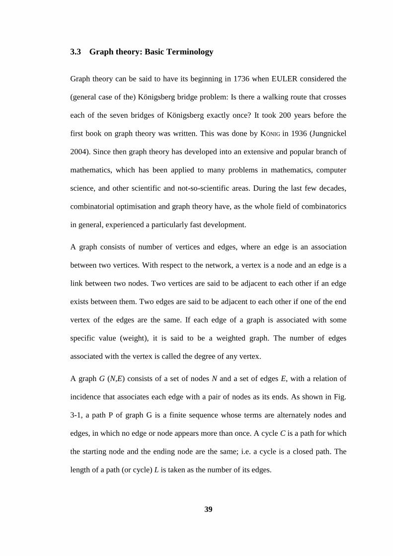
39
3.3 Graph theory: Basic Terminology
Graph theory can be said to have its beginning in 1736 when EULER considered the
(general case of the) Königsberg bridge problem: Is there a walking route that crosses
each of the seven bridges of Königsberg exactly once? It took 200 years before the
first book on graph theory was written. This was done by KÖNIG in 1936 (Jungnickel
2004). Since then graph theory has developed into an extensive and popular branch of
mathematics, which has been applied to many problems in mathematics, computer
science, and other scientific and not-so-scientific areas. During the last few decades,
combinatorial optimisation and graph theory have, as the whole field of combinatorics
in general, experienced a particularly fast development.
A graph consists of number of vertices and edges, where an edge is an association
between two vertices. With respect to the network, a vertex is a node and an edge is a
link between two nodes. Two vertices are said to be adjacent to each other if an edge
exists between them. Two edges are said to be adjacent to each other if one of the end
vertex of the edges are the same. If each edge of a graph is associated with some
specific value (weight), it is said to be a weighted graph. The number of edges
associated with the vertex is called the degree of any vertex.
A graph G (N,E) consists of a set of nodes N and a set of edges E, with a relation of
incidence that associates each edge with a pair of nodes as its ends. As shown in Fig.
3-1, a path P of graph G is a finite sequence whose terms are alternately nodes and
edges, in which no edge or node appears more than once. A cycle C is a path for which
the starting node and the ending node are the same; i.e. a cycle is a closed path. The
length of a path (or cycle) L is taken as the number of its edges.
40
Figure 3-1 A path and a cycle on directed graphs
3.4 Shortest Path Problems
In the graph theory, as shown in Fig. 3-1, the shortest path problem is the problem of
finding a path from a specified node called the source to a second specified node
called the destination (or target), such that the sum of the weights (or lengths) of its
constituent edges is minimised. It is relevant to a wide variety of real world
applications, such as in telephone routing, material distribution, salesperson routing,
investment strategies, and personnel scheduling. The shortest path problem is an NP-
hard combinatorial optimisation problem, which means that it is believed that they
cannot be solved to optimality within polynomially bounded computation time. To
practically solve large instances, one often has to use heuristics that returns near-
optimal solutions in a relatively short time (Lawler 2001; Korte and Vygen 2012).
Consider a weighted undirected graph G (N, E). Let 𝑛 = 𝑁 and 𝑚 = 𝐸 . Each edge
eij ∈ E is assigned a cost (or length) of cij. If cij has multiple criteria, the problem is
called a multi-objective shortest path problem. In this case the edge eij has associated
values 𝑐𝑖𝑗𝑘 , in which k ∈ {1, 2,…, r} for each criterion k=1, 2, …, r. Obviously, for
undirected graphs 𝑐𝑖𝑗𝑘 = 𝑐𝑗𝑖
𝑘 . The adjacency set A(i) for node i is the set of all edges
41
incident from i, that is A(i)={(i,j)ǀ(i,j)∈E}. The integer programming formulation for
the multi-objective shortest path problem from Node s to Node t can be given as
follows (Reinhardt and Pisinger 2011):
𝑚𝑖𝑛 𝑓 = 𝑐𝑖𝑗1
𝑖 ,𝑗∈𝑉
𝑒𝑖𝑗 , 𝑐𝑖𝑗2
𝑖 ,𝑗∈𝑉
𝑒𝑖𝑗 , … , 𝑐𝑖𝑗𝑟
𝑖 ,𝑗∈𝑉
𝑒𝑖𝑗 (3-1)
𝑒𝑖𝑗 ∈ 𝐸 ∶ 𝑒𝑖𝑗 = 1 𝑖𝑓 𝐸𝑑𝑔𝑒 𝑒𝑖𝑗 𝑖𝑠 𝑐𝑜𝑠𝑒𝑛
0 𝑖𝑓 𝐸𝑑𝑔𝑒 𝑒𝑖𝑗 𝑖𝑠 𝑛𝑜𝑡 𝑐𝑜𝑠𝑒𝑛 (3-2)
𝑖 ∈ 𝑁 − 𝑠, 𝑡 : 𝑒𝑖𝑗
𝑗
− 𝑒𝑘𝑖
𝑘
= 0 (3-3)
𝑖, 𝑗 ∈ 𝑁: 𝑒𝑠𝑖
𝑖
− 𝑒𝑗𝑠
𝑗
= 1 (3-4)
𝑖, 𝑗 ∈ 𝑁: 𝑒𝑖𝑡
𝑖
− 𝑒𝑡𝑗
𝑗
= 1 (3-5)
Equation (3-1) represents the objective and Eq. (3-2) defines the binary variable 𝒆𝒊𝒋.
Equations (3-3) through (3-5) are the constraints.
Equation (3-3), as an ordinary flow conservation constraint, states that for all nodes
except for the source and target points, the edges leaving them are equal to the edges
entering them. Equations (3-4) and (3-5) state that the difference between the number
of edges leaving the source and target points and the number of edges entering them,
respectively, is one. In other words, the edges are not on a cycle. In a generalised form
of the problem, called the all-pairs shortest path problem, the shortest paths from every
42
possible source to every possible target are determined in order to form the shortest
path matrix that gives the shortest path between every pair of vertices.
The multi-objective shortest path problem consists in finding in a network with vector
weights on the edges optimal paths. Most published papers usually consider the
problem with specified starting and ending node, or from a given starting node to all
other nodes. The shortest path problem belongs to the most widely studied multi-
objective problems (Martins 1996). Most problems in this category are NP -complete.
3.4.1 Shortest Path Problem for Column Layout Design
Consider a reinforced concrete frame with N spans. The aim is to find the optimum
column layout locations of the RC frame which leads to the optimum spans of the
frame, as shown in Fig. 3-2, in a way that optimizes the relevant costs. The height of
stories, that is column lengths, is considered determinate and constant.
In order to deal with the column layout design as a combinatorial optimisation
problem, as the first step, the domain needs to be discretised. As such the directed
graph is defined assuming that span lengths are bounded in [Lmin Lmax] in either
direction (Lmin and Lmax can get different values for each span) with intervals
(accuracy) equal to ε. That is, each Li rests in the set of {Lmin , Lmin + ε, Lmin + 2ε ,…,
Lmax - ε , Lmax}. Obviously, the smaller ε is, the more accurate the results will be and
the more running time the algorithm needs. As shown in Fig. 3-2, a directed graph is
defined, which is used as the construction graph for ACO algorithm, to demonstrate
the column layout of the 2D RC frame. The members of the graph denote spans. In
order for the graph to stand for the structure layout, the total number of spans and the
number of nodes need to be N and (N+1) respectively. Hence, the construction graph
is defined as a graph with N nodes and ((Lmax -Lmin)/ ε *N) edges. Each pair of nodes
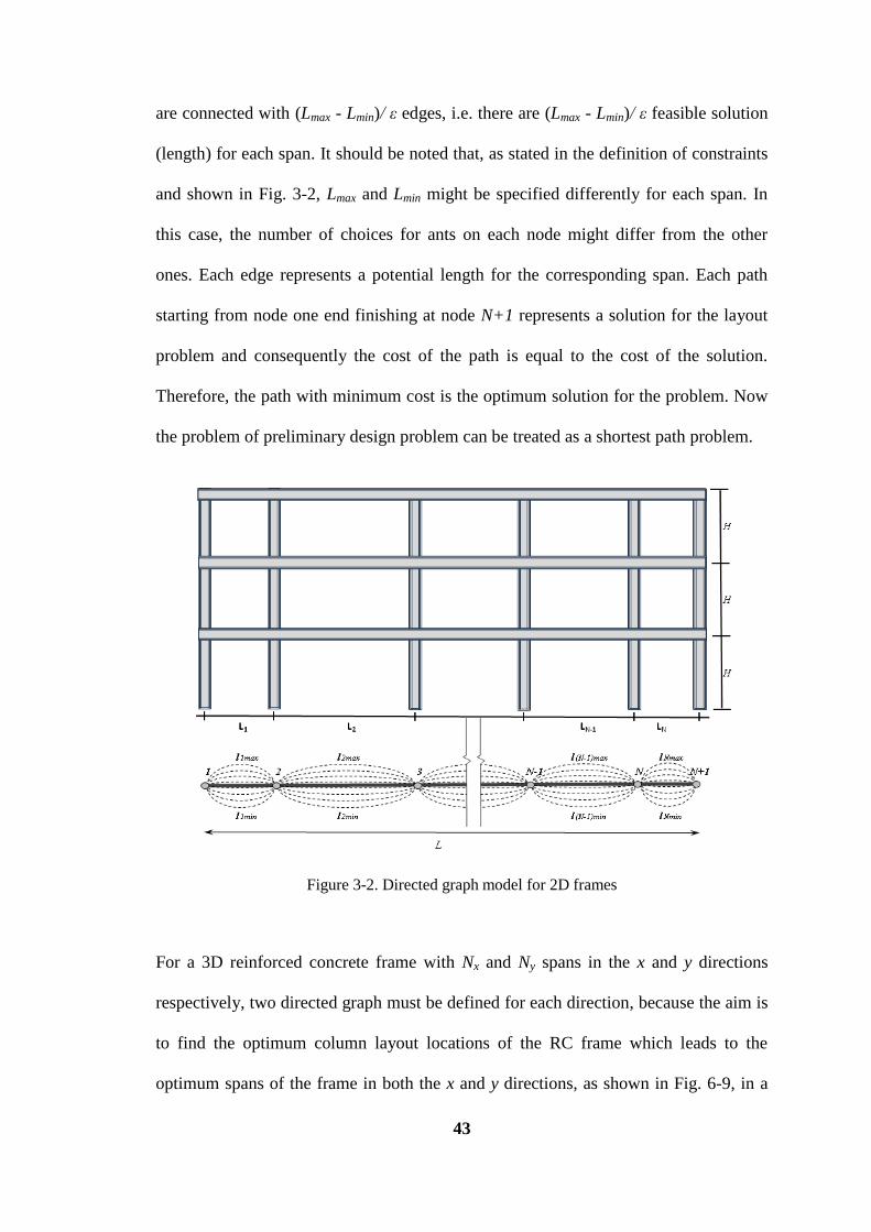
43
are connected with (Lmax - Lmin)/ ε edges, i.e. there are (Lmax - Lmin)/ ε feasible solution
(length) for each span. It should be noted that, as stated in the definition of constraints
and shown in Fig. 3-2, Lmax and Lmin might be specified differently for each span. In
this case, the number of choices for ants on each node might differ from the other
ones. Each edge represents a potential length for the corresponding span. Each path
starting from node one end finishing at node N+1 represents a solution for the layout
problem and consequently the cost of the path is equal to the cost of the solution.
Therefore, the path with minimum cost is the optimum solution for the problem. Now
the problem of preliminary design problem can be treated as a shortest path problem.
Figure 3-2. Directed graph model for 2D frames
For a 3D reinforced concrete frame with Nx and Ny spans in the x and y directions
respectively, two directed graph must be defined for each direction, because the aim is
to find the optimum column layout locations of the RC frame which leads to the
optimum spans of the frame in both the x and y directions, as shown in Fig. 6-9, in a
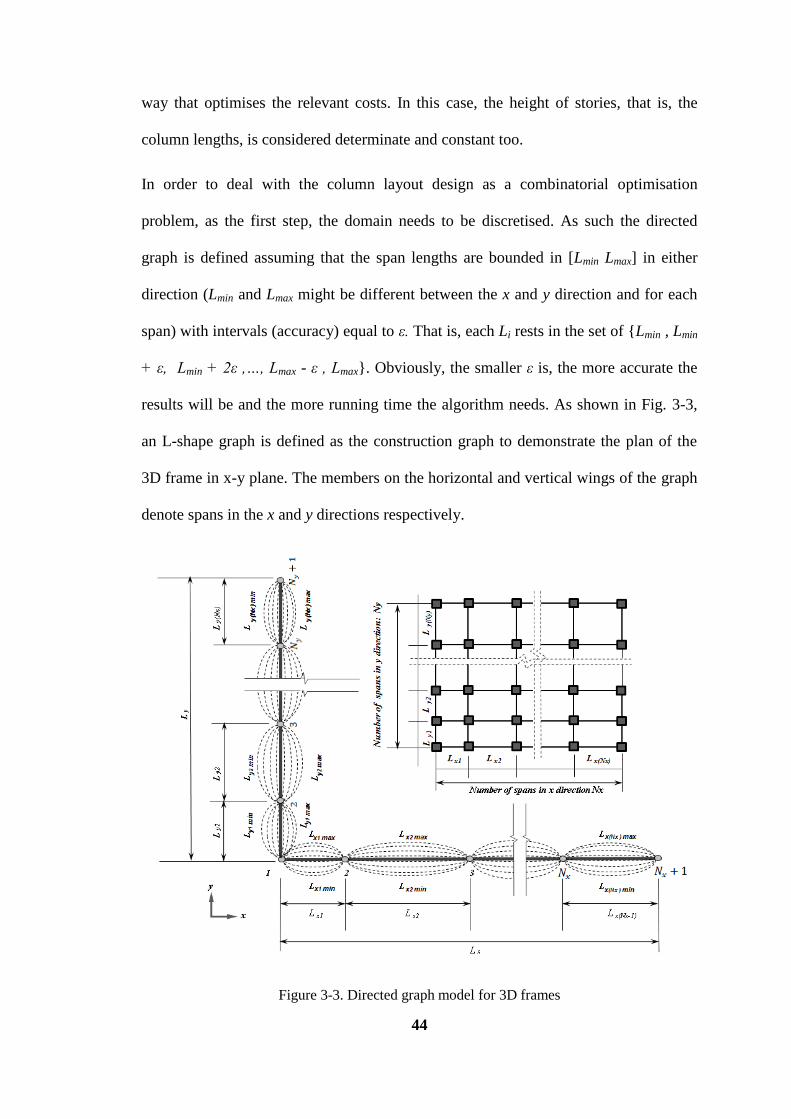
44
way that optimises the relevant costs. In this case, the height of stories, that is, the
column lengths, is considered determinate and constant too.
In order to deal with the column layout design as a combinatorial optimisation
problem, as the first step, the domain needs to be discretised. As such the directed
graph is defined assuming that the span lengths are bounded in [Lmin Lmax] in either
direction (Lmin and Lmax might be different between the x and y direction and for each
span) with intervals (accuracy) equal to ε. That is, each Li rests in the set of {Lmin , Lmin
+ ε, Lmin + 2ε ,…, Lmax - ε , Lmax}. Obviously, the smaller ε is, the more accurate the
results will be and the more running time the algorithm needs. As shown in Fig. 3-3,
an L-shape graph is defined as the construction graph to demonstrate the plan of the
3D frame in x-y plane. The members on the horizontal and vertical wings of the graph
denote spans in the x and y directions respectively.
Figure 3-3. Directed graph model for 3D frames
45
In order for the graph to stand for the structure layout, the total number of spans and
the number of nodes need to be Nx+Ny and (Nx+Ny+1) respectively, in which Nx and
Ny are the total number of spans in the x and y directions respectively. Hence, the
construction graph is defined as a graph with Nx+Ny+1 nodes and ((Lmax -Lmin)/ ε
*Nx)+((Lmax - Lmin)/ ε *Ny) edges. Each pair of nodes are connected with (Lmax - Lmin)/ ε
edges, i.e. there are (Lmax - Lmin)/ ε feasible solution for each span. It should be pointed
out that, as stated in the definition of constraints and shown in Fig. 3-3, Lmax and Lmin
might be specified differently for each span. In this case, the number of choices for
ants on each node might differ from the other ones. Therefore, the paths with
minimum cost, for each direction, are the optimum solution for the problem.
3.5 Knapsack Problems
Knapsacks are basic problems in combinatorial optimisation, and applications arise
whenever we want to select an optimum subset of bounded weight from a set of
elements each of which has a weight and a profit. There are a number of items
available, each consumes a known amount of the resource and contributes a known
benefit. Items must be selected in a way that maximises the total benefit without
exceeding the given amount of the resource. Knapsack problems have been intensively
studied in the past few decades (Kellerer et al. 2004), because of immediate
applications in industry and management. Furthermore, knapsack problems arise in
many practical situations and frequently occur by relaxing the various integer-
programming problems. A variety of complex optimisation problems can be solved
through a series of knapsack-type problems (Martello and Toth 1990).
46
The knapsack problem is one of the fundamental NP-complete combinatorial
optimisation problems. The knapsack problem (KP) and its multi-dimensional version
(MKP) are basic problems in combinatorial optimisation. Comprehensive surveys
have been carried out on multi-objective multi-dimensional knapsack problems and
Quadratic knapsack problems by Lust et al. (2012) and Pisinger (2007).
There are several problems from the family of knapsack problems that are considered
in this thesis. In all variants of the problem it is assumed that there are some items with
a given profit and weight, which are packed in one or more knapsack of a limited
capacity. Knapsack problems are NP-hard, which means that it is strongly believed
that they cannot be solved to optimality within polynomially bounded computation
time. To practically solve large instances, one often has to use heuristics that returns
near-optimal solutions in a relatively short time.
Given a set of items i∈ I={1,2,…,n} with associated a vector of weights ri and a profit
bi, the knapsack problem is the problem of selecting a subset of items from I in such a
way that they fit into a knapsack of limited capacity a, and maximise the sum of
profits of the chosen items. Let yi be a variable associated with item i, which is 1 if i is
added to the knapsack and 0 otherwise. The general knapsack problem can be
formulated as
𝑚𝑎𝑥 𝑓 = 𝑏𝑖𝑦𝑖
n
i=1
(3-6)
𝑟𝑖𝑦𝑖
n
i=1
≤ 𝑎 (3-7)
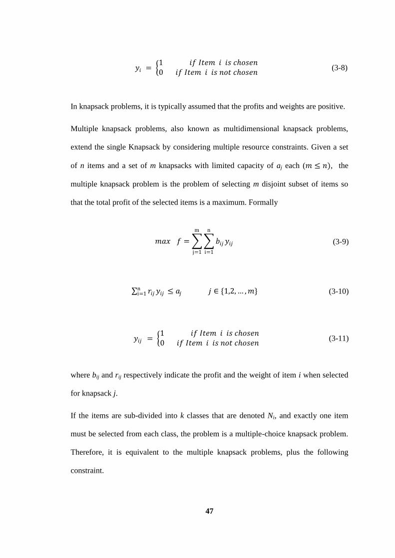
47
𝑦𝑖 = 1 𝑖𝑓 𝐼𝑡𝑒𝑚 𝑖 𝑖𝑠 𝑐𝑜𝑠𝑒𝑛 0 𝑖𝑓 𝐼𝑡𝑒𝑚 𝑖 𝑖𝑠 𝑛𝑜𝑡 𝑐𝑜𝑠𝑒𝑛
(3-8)
In knapsack problems, it is typically assumed that the profits and weights are positive.
Multiple knapsack problems, also known as multidimensional knapsack problems,
extend the single Knapsack by considering multiple resource constraints. Given a set
of n items and a set of m knapsacks with limited capacity of aj each (𝑚 ≤ 𝑛), the
multiple knapsack problem is the problem of selecting m disjoint subset of items so
that the total profit of the selected items is a maximum. Formally
𝑚𝑎𝑥 𝑓 = 𝑏𝑖𝑗 𝑦𝑖𝑗
n
i=1
m
j=1
(3-9)
𝑟𝑖𝑗 𝑦𝑖𝑗ni=1 ≤ 𝑎𝑗 𝑗 ∈ {1,2, … , 𝑚} (3-10)
𝑦𝑖𝑗 = 1 𝑖𝑓 𝐼𝑡𝑒𝑚 𝑖 𝑖𝑠 𝑐𝑜𝑠𝑒𝑛 0 𝑖𝑓 𝐼𝑡𝑒𝑚 𝑖 𝑖𝑠 𝑛𝑜𝑡 𝑐𝑜𝑠𝑒𝑛
(3-11)
where bij and rij respectively indicate the profit and the weight of item i when selected
for knapsack j.
If the items are sub-divided into k classes that are denoted Ni, and exactly one item
must be selected from each class, the problem is a multiple-choice knapsack problem.
Therefore, it is equivalent to the multiple knapsack problems, plus the following
constraint.
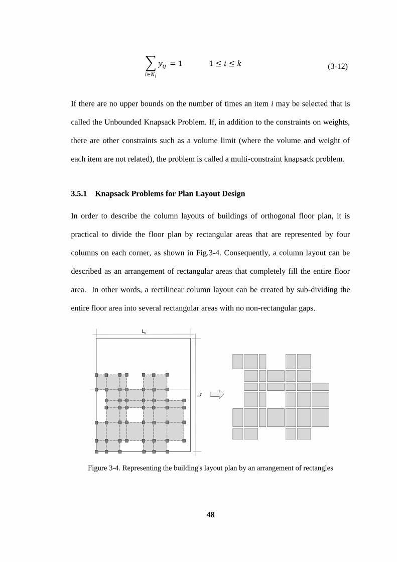
48
𝑦𝑖𝑗
𝑖∈𝑁𝑖
= 1 1 ≤ 𝑖 ≤ 𝑘 (3-12)
If there are no upper bounds on the number of times an item i may be selected that is
called the Unbounded Knapsack Problem. If, in addition to the constraints on weights,
there are other constraints such as a volume limit (where the volume and weight of
each item are not related), the problem is called a multi-constraint knapsack problem.
3.5.1 Knapsack Problems for Plan Layout Design
In order to describe the column layouts of buildings of orthogonal floor plan, it is
practical to divide the floor plan by rectangular areas that are represented by four
columns on each corner, as shown in Fig.3-4. Consequently, a column layout can be
described as an arrangement of rectangular areas that completely fill the entire floor
area. In other words, a rectilinear column layout can be created by sub-dividing the
entire floor area into several rectangular areas with no non-rectangular gaps.
Figure 3-4. Representing the building's layout plan by an arrangement of rectangles
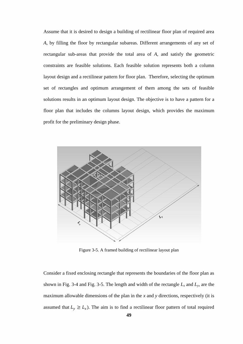
49
Assume that it is desired to design a building of rectilinear floor plan of required area
A, by filling the floor by rectangular subareas. Different arrangements of any set of
rectangular sub-areas that provide the total area of A, and satisfy the geometric
constraints are feasible solutions. Each feasible solution represents both a column
layout design and a rectilinear pattern for floor plan. Therefore, selecting the optimum
set of rectangles and optimum arrangement of them among the sets of feasible
solutions results in an optimum layout design. The objective is to have a pattern for a
floor plan that includes the columns layout design, which provides the maximum
profit for the preliminary design phase.
Figure 3-5. A framed building of rectilinear layout plan
Consider a fixed enclosing rectangle that represents the boundaries of the floor plan as
shown in Fig. 3-4 and Fig. 3-5. The length and width of the rectangle Lx and Ly, are the
maximum allowable dimensions of the plan in the x and y directions, respectively (it is
assumed that 𝐿𝑦 ≥ 𝐿𝑥). The aim is to find a rectilinear floor pattern of total required

50
area A, and the corresponding column layout with maximum profit, inside the
enclosing rectangle.
A rectilinear pattern is formed of a number of rectangular subareas. Assume that there
is a set of rectangles of various lengths and widths, which meet the geometric
requirements, such as maximum and minimum spans lengths. These rectangles
represent the relative location of four columns on their corners and the floor (or slab)
surrounded by them. Rectangles are used to form a rectilinear shape of area A. The
problem changes to select a set of rectangles of total area A and an appropriate
arrangement of them that maximise the profit (objective function) and meet the
constraints. The constraints are as follows:
The rectangles were placed onto the floor plan with their four sides parallel to the x
and y-axis. That is, each edge of a rectangle is parallel to an edge of the enclosing
rectangle.
There is no overlapping for any two rectangles.
To have all the columns on a grid pattern, the edges shared by any two adjacent
rectangles have the same length. This condition prevents the layout plan from having
columns that are off centre and places all the columns on a grid pattern as shown if
Fig. 3-4.
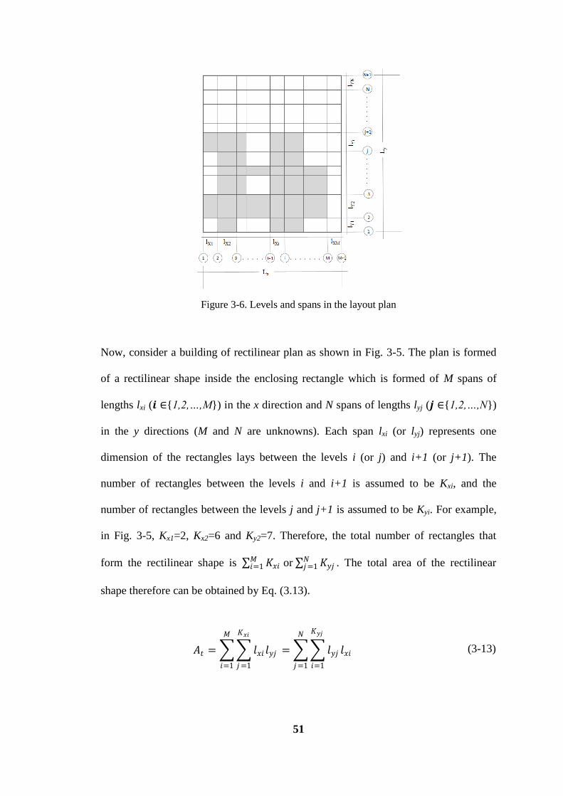
51
Figure 3-6. Levels and spans in the layout plan
Now, consider a building of rectilinear plan as shown in Fig. 3-5. The plan is formed
of a rectilinear shape inside the enclosing rectangle which is formed of M spans of
lengths lxi (𝒊 ∈{1,2,…,M}) in the x direction and N spans of lengths lyj (𝒋 ∈{1,2,…,N})
in the y directions (M and N are unknowns). Each span lxi (or lyj) represents one
dimension of the rectangles lays between the levels i (or j) and i+1 (or j+1). The
number of rectangles between the levels i and i+1 is assumed to be Kxi, and the
number of rectangles between the levels j and j+1 is assumed to be Kyi. For example,
in Fig. 3-5, Kx1=2, Kx2=6 and Ky2=7. Therefore, the total number of rectangles that
form the rectilinear shape is 𝐾𝑥𝑖𝑀𝑖=1 or 𝐾𝑦𝑗
𝑁𝑗=1 . The total area of the rectilinear
shape therefore can be obtained by Eq. (3.13).
𝐴𝑡 = 𝑙𝑥𝑖 𝑙𝑦𝑗
𝐾𝑥𝑖
𝑗 =1
𝑀
𝑖=1
= 𝑙𝑦𝑗 𝑙𝑥𝑖
𝐾𝑦𝑗
𝑖=1
𝑁
𝑗=1
(3-13)
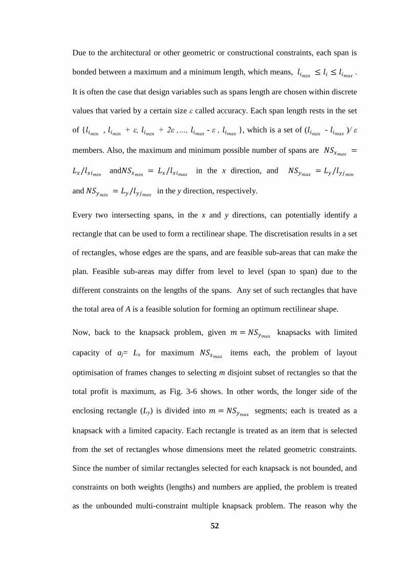
52
Due to the architectural or other geometric or constructional constraints, each span is
bonded between a maximum and a minimum length, which means, 𝑙𝑖𝑚𝑖𝑛≤ 𝑙𝑖 ≤ 𝑙𝑖𝑚𝑎𝑥
.
It is often the case that design variables such as spans length are chosen within discrete
values that varied by a certain size ε called accuracy. Each span length rests in the set
of {𝑙𝑖𝑚𝑖𝑛 , 𝑙𝑖𝑚𝑖𝑛
+ ε, 𝑙𝑖𝑚𝑖𝑛 + 2ε ,…, 𝑙𝑖𝑚𝑎𝑥
- ε , 𝑙𝑖𝑚𝑎𝑥}, which is a set of (𝑙𝑖𝑚𝑖𝑛
- 𝑙𝑖𝑚𝑎𝑥)/ ε
members. Also, the maximum and minimum possible number of spans are 𝑁𝑆𝑥𝑚𝑎𝑥=
𝐿𝑥/𝑙𝑥𝑖𝑚𝑖𝑛 and𝑁𝑆𝑥𝑚𝑖𝑛= 𝐿𝑥/𝑙𝑥𝑖𝑚𝑎𝑥 in the x direction, and 𝑁𝑆𝑦𝑚𝑎𝑥
= 𝐿𝑦 /𝑙𝑦𝑗𝑚𝑖𝑛
and 𝑁𝑆𝑦𝑚𝑖𝑛= 𝐿𝑦 /𝑙𝑦𝑗𝑚𝑎𝑥 in the y direction, respectively.
Every two intersecting spans, in the x and y directions, can potentially identify a
rectangle that can be used to form a rectilinear shape. The discretisation results in a set
of rectangles, whose edges are the spans, and are feasible sub-areas that can make the
plan. Feasible sub-areas may differ from level to level (span to span) due to the
different constraints on the lengths of the spans. Any set of such rectangles that have
the total area of A is a feasible solution for forming an optimum rectilinear shape.
Now, back to the knapsack problem, given 𝑚 = 𝑁𝑆𝑦𝑚𝑎𝑥 knapsacks with limited
capacity of aj= Lx for maximum 𝑁𝑆𝑥𝑚𝑎𝑥 items each, the problem of layout
optimisation of frames changes to selecting m disjoint subset of rectangles so that the
total profit is maximum, as Fig. 3-6 shows. In other words, the longer side of the
enclosing rectangle (Ly) is divided into 𝑚 = 𝑁𝑆𝑦𝑚𝑎𝑥 segments; each is treated as a
knapsack with a limited capacity. Each rectangle is treated as an item that is selected
from the set of rectangles whose dimensions meet the related geometric constraints.
Since the number of similar rectangles selected for each knapsack is not bounded, and
constraints on both weights (lengths) and numbers are applied, the problem is treated
as the unbounded multi-constraint multiple knapsack problem. The reason why the
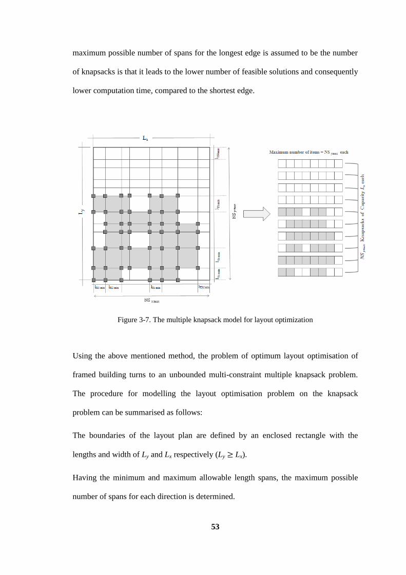
53
maximum possible number of spans for the longest edge is assumed to be the number
of knapsacks is that it leads to the lower number of feasible solutions and consequently
lower computation time, compared to the shortest edge.
Figure 3-7. The multiple knapsack model for layout optimization
Using the above mentioned method, the problem of optimum layout optimisation of
framed building turns to an unbounded multi-constraint multiple knapsack problem.
The procedure for modelling the layout optimisation problem on the knapsack
problem can be summarised as follows:
The boundaries of the layout plan are defined by an enclosed rectangle with the
lengths and width of Ly and Lx respectively (Ly ≥ Lx).
Having the minimum and maximum allowable length spans, the maximum possible
number of spans for each direction is determined.
54
Defining a desirable accuracy, a set of rectangles is formed by discretising the domain
for each span. This set contains the rectangles of all allowable dimensions that
represent the set of items. The sets can be independently formed for each span due to
the different limitations on lengths.
The number of knapsacks m is set to the maximum number of spans in the longest
edge of the enclosing rectangle.
As a bi-constraint problem, two constraints are set for the knapsacks capacity. The
first one is the constraint on the weight (length), which is set to the width of the
enclosing rectangle. The second one is the constraint on the number of items, which is
set to the maximum number of spans in the shortest edge of the enclosing rectangle.
The profit can be defined as the inverse of cost and/or the inverse of the lateral
displacement, or any other objectives depending on the problem.
By defining the objective and having a set of items, a set of knapsacks and their
capacity, the layout optimisation of rectilinear frames can be formulated by Eqs. (3-9)
through (3-11).
There are some limitations when selecting a rectangle from the set. In order to have all
the columns on level i, in a row and not to have off-centre columns, when the first
rectangle (item) is chosen for knapsack i, all the following rectangles must have the
same width. In other words, selecting the first rectangle for each span is equivalent to
specifying a length to the span, and all the following rectangles are selected from a
subset of rectangles that are identical in width. Such a constraint makes the problem
similar to multiple-choice knapsack problem. That is, rectangles can be sub-divided
into some classes such that rectangles with identical length are put in the same class.
Then, exactly one rectangle must be selected from each class for a particular knapsack.
55
When defining the knapsacks for each row in the y direction, it should be noted that
each item in each knapsack is corresponding to a rectangle in the plan. In other words,
the Item i in the Knapsack j is corresponding to the Rectangle ij, which is surrounded
by the Level i and i+1 in the x direction and Level j and j+1 in the y direction.
Therefore, if a rectangle of area rij is selected for the vacant as the Item ij (Item i in the
Knapsack j) it consumes one of the total vacant capacities of the knapsack j and a
weight of rij from the total weight capacity aij. While if no rectangle is selected for the
Item ij it means that that subarea is void. In this case the void area consumes one of
the total vacant capacities of the Knapsack j and a weight of zero from the total weight
capacity.
In order to reach practical outcomes, for example to prevent the plan being split into
two or more unconnected parts, or in case of preferences for some particular shapes,
additional constraints can be imposed on the capacity of each knapsack or the location
of voids. In the following some common special cases are considered.
Depending on the desired geometric layout design, three widespread special cases
were considered to simplify the application of the method. Each case can be treated as
a certain type of knapsack problem. It should be noted that the general case mentioned
above can cover the entire following cases by adding some constraints to the problem.
Nevertheless, based on the authors experience and the instances already solved,
employing the classification bellow for some special cases, and employing their own
specified methods of solution makes it easier to deal with the corresponding layout
optimisation problem.
Case 1: A rectangular layout pattern where the number of spans in each direction is
fixed and the aim is to determine the lengths of the spans: Consider a building with a
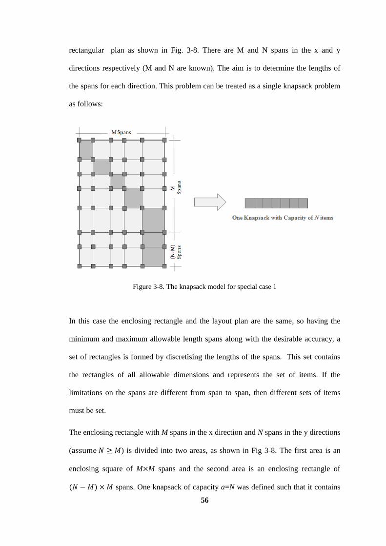
56
rectangular plan as shown in Fig. 3-8. There are M and N spans in the x and y
directions respectively (M and N are known). The aim is to determine the lengths of
the spans for each direction. This problem can be treated as a single knapsack problem
as follows:
Figure 3-8. The knapsack model for special case 1
In this case the enclosing rectangle and the layout plan are the same, so having the
minimum and maximum allowable length spans along with the desirable accuracy, a
set of rectangles is formed by discretising the lengths of the spans. This set contains
the rectangles of all allowable dimensions and represents the set of items. If the
limitations on the spans are different from span to span, then different sets of items
must be set.
The enclosing rectangle with M spans in the x direction and N spans in the y directions
(assume 𝑁 ≥ 𝑀) is divided into two areas, as shown in Fig 3-8. The first area is an
enclosing square of M×M spans and the second area is an enclosing rectangle of
(𝑁 − 𝑀) × 𝑀 spans. One knapsack of capacity a=N was defined such that it contains
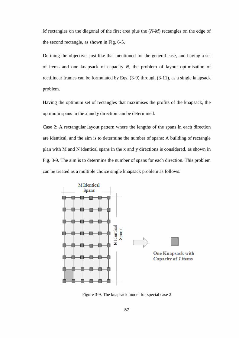
57
M rectangles on the diagonal of the first area plus the (N-M) rectangles on the edge of
the second rectangle, as shown in Fig. 6-5.
Defining the objective, just like that mentioned for the general case, and having a set
of items and one knapsack of capacity N, the problem of layout optimisation of
rectilinear frames can be formulated by Eqs. (3-9) through (3-11), as a single knapsack
problem.
Having the optimum set of rectangles that maximises the profits of the knapsack, the
optimum spans in the x and y direction can be determined.
Case 2: A rectangular layout pattern where the lengths of the spans in each direction
are identical, and the aim is to determine the number of spans: A building of rectangle
plan with M and N identical spans in the x and y directions is considered, as shown in
Fig. 3-9. The aim is to determine the number of spans for each direction. This problem
can be treated as a multiple choice single knapsack problem as follows:
Figure 3-9. The knapsack model for special case 2
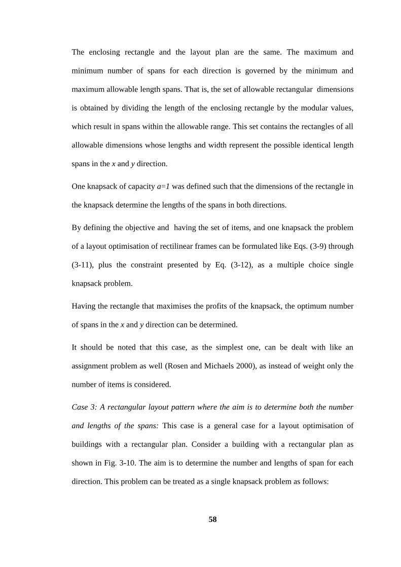
58
The enclosing rectangle and the layout plan are the same. The maximum and
minimum number of spans for each direction is governed by the minimum and
maximum allowable length spans. That is, the set of allowable rectangular dimensions
is obtained by dividing the length of the enclosing rectangle by the modular values,
which result in spans within the allowable range. This set contains the rectangles of all
allowable dimensions whose lengths and width represent the possible identical length
spans in the x and y direction.
One knapsack of capacity a=1 was defined such that the dimensions of the rectangle in
the knapsack determine the lengths of the spans in both directions.
By defining the objective and having the set of items, and one knapsack the problem
of a layout optimisation of rectilinear frames can be formulated like Eqs. (3-9) through
(3-11), plus the constraint presented by Eq. (3-12), as a multiple choice single
knapsack problem.
Having the rectangle that maximises the profits of the knapsack, the optimum number
of spans in the x and y direction can be determined.
It should be noted that this case, as the simplest one, can be dealt with like an
assignment problem as well (Rosen and Michaels 2000), as instead of weight only the
number of items is considered.
Case 3: A rectangular layout pattern where the aim is to determine both the number
and lengths of the spans: This case is a general case for a layout optimisation of
buildings with a rectangular plan. Consider a building with a rectangular plan as
shown in Fig. 3-10. The aim is to determine the number and lengths of span for each
direction. This problem can be treated as a single knapsack problem as follows:
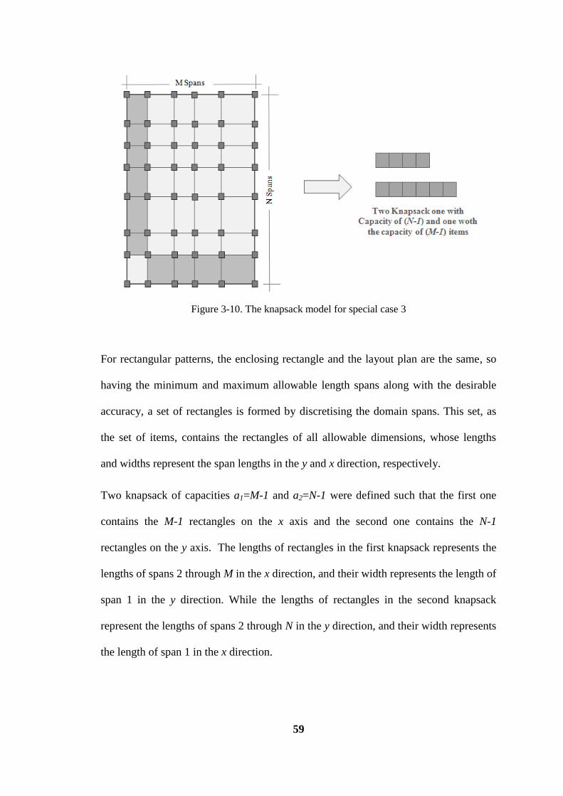
59
Figure 3-10. The knapsack model for special case 3
For rectangular patterns, the enclosing rectangle and the layout plan are the same, so
having the minimum and maximum allowable length spans along with the desirable
accuracy, a set of rectangles is formed by discretising the domain spans. This set, as
the set of items, contains the rectangles of all allowable dimensions, whose lengths
and widths represent the span lengths in the y and x direction, respectively.
Two knapsack of capacities a1=M-1 and a2=N-1 were defined such that the first one
contains the M-1 rectangles on the x axis and the second one contains the N-1
rectangles on the y axis. The lengths of rectangles in the first knapsack represents the
lengths of spans 2 through M in the x direction, and their width represents the length of
span 1 in the y direction. While the lengths of rectangles in the second knapsack
represent the lengths of spans 2 through N in the y direction, and their width represents
the length of span 1 in the x direction.
60
By defining the objective and having the set of items and two knapsacks, the problem
of a layout optimisation of rectangular frames can be formulated by Eqs. (6-9) through
(6-11), as a multiple knapsack (bi-knapsack) problem.
Having the optimum set of rectangles that maximises the profits of the knapsack, the
optimum spans in the x and y direction can be determined.
Just like the general case, the only constraint in this case, in order not to have the
columns off centre, was that when the first rectangle was selected for each knapsack,
the following knapsacks must have the same width, which gives the problem a
multiple-choice nature.
In all cases, in addition to the aforementioned constraints, in case of some other
architectural or structural preferences such as some special plan shapes or symmetric
plans (for example as a result of minimising the eccentricity of the mass centre for
lateral loads), the constraints can easily be added to the rectangles' selection criteria.
3.6 Randomised Search Heuristics and Methaheuristics
Randomised search heuristics have been widely applied to complex engineering
problems as well as those from combinatorial optimization. Randomised search
heuristics are general-purpose algorithms, which often yield good solutions for
problems whose structure is not known very well. Evolutionary algorithms (EAs)
belonging to this class of algorithms have become quite popular since the ‘60s of the
last century. Their main advantage is their fast application to different problem
domains. Using an appropriate encoding for a given problem and some standard
variation operators together with a fitness function for the considered problems, one
can often come up with good solutions for the problem. Evolutionary algorithms have

61
been widely applied to complex engineering problems as well as problems from
combinatorial optimisation. In the case of a complex engineering problem the structure
of the problem is often not known which means that the quality of a certain parameter
setting can only be evaluated by experiments or simulations.
A randomised search heuristic is a problem-independent algorithm to solve problems
from a considered search space, although it might have modules that are adjusted to
the considered problem or are combined with problem-dependent algorithms.
Independence from the considered problem distinguishes randomised search heuristics
from problem dependent algorithms developed and analysed in the classical algorithm
community (Neumann 2006). In contrast to the classical approach to algorithms where
one designs an algorithm with the view to prove the bounds on the runtime and/or
approximation quality in mind, randomised search heuristics are general-purpose
algorithms.
In the case of combinatorial optimisation, much is often known about the structure of a
given problem and the function to be optimised. Nevertheless it is often difficult to
obtain good solutions for such problems, especially if the problem is new and there are
not enough resources (such as time, knowledge, money) to design specific algorithms
for the given problem. In this case, the application of randomized search heuristics
often yields satisfying results (Neumann 2006). We take a closer look at Ant Colony
Optimisation as a bio-inspired randomised search heuristic Section 3.7.
Metaheuristic algorithms use a certain trade-off of randomisation and local search.
Randomisation provides a good way to move away from local search to a search on
the global scale, and therefore almost all metaheuristic algorithms tend to be suitable
for global optimisation. It is a way by trial and error to produce acceptable solutions to
62
a complex problem in a reasonably practical time. The complexity of the problem of
interest makes it impossible to search every possible solution or combination, the aim
is to find a good feasible solution in an acceptable time scale. There is no guarantee
that the best solutions can be found, and we do not even know whether an algorithm
will work and why if it does work. The idea is to have an efficient but practical
algorithm that will work most the time and is able to produce good quality solutions.
Modern metaheuristic algorithms such as the ant colony optimisation and harmony
search start to demonstrate their power in dealing with tough optimisation problems
and even NP-hard problems (Yang 2010).
It is quite apparent that large numbers of combinations are possible for designing a
frame depending upon the total number of practical solutions available. In recent
years novel and innovative search techniques have developed that make use of ideas
taken from nature and do not suffer the discrepancies of mathematical programming
based optimum design methods. Comprehensive reviews on stochastic search
techniques based on natural phenomena have been carried out by Saka (2007), and
Saka and Dogan (2012). The basic idea behind these techniques is to simulate natural
phenomena such as survival of the fittest, immune system, swarm intelligence, etc.,
into a numerical algorithm. These methods are non-traditional stochastic search and
optimisation methods that are very suitable, and powerful at obtaining solutions for
combinatorial optimisation problems. They do not require the derivatives of the
objective function and constraints and they use probabilistic transition rules, not
deterministic rules (Saka 2007).
Metaheuristic is a class of stochastic methods, although the recent trend tends to name
all stochastic algorithms with randomisation and local search as metaheuristic. An
important class of metaheuristics are ones inspired by nature, including genetic
63
algorithms (GA), particle swarm optimisation (PSO), simulated annealing (SA), ant
colony optimisation (ACO), bee algorithms (BA), harmony search (HS), firefly
algorithms (FA), photo synthetic algorithm (PA), enzyme algorithm (EA), and Tabu
search. The 1960s and 1970s were the two most important decades for the
development of evolutionary algorithms, although the search to find computationally
more efficient metaheuristic algorithms has gained pace since 2000. A brief history of
metaheuristic has been presented in (Yang 2010).
To find an optimal solution to an optimisation problem is often a very challenging
task, and one that depends on the choice and correct use of the right algorithm. The
choice of an algorithm may depend on the type of problem, the algorithms available,
computational resources and time constraints. For large scale, non-linear, global
optimisation problems, there is often no agreed guideline for the choice of algorithm
and in many cases, there is no efficient algorithm. For hard optimisation problems,
especially for non-deterministic polynomial-time hard, or NP-hard optimisation
problems, there is no efficient algorithm at all (Gandomi et al. 2013).
Various algorithms may be used for solving optimisation problems, although
conventional or classic algorithms are mostly deterministic. For instance, the simplex
method in linear programming is deterministic. Some other deterministic optimisation
algorithms such as the Newton-Raphson algorithm use gradient information and are
called gradient-based algorithms. Non-gradient-based, or gradient-free/derivative-free,
algorithms only use the function values; they do not use any derivative.
Heuristic and metaheuristic are the main types of the stochastic algorithms. The
difference between Heuristic and metaheuristic algorithms is negligible. Heuristic
means ‗to find‘ or ‗to discover by trial and error‘. Quality solutions to a tough
64
optimisation problem can be found in a reasonable amount of time, but there is no
guarantee that optimal solutions can be reached, indeed it is hoped that these
algorithms work most of the time, but not necessarily all the time. This is good when
good solutions which are easily reachable are needed, and not necessarily the best
solutions (Gandomi et al. 2013).
Metaheuristic optimisation algorithms are often inspired from nature. According to the
source of inspiration for metaheuristic algorithms, they can be classified into different
categories. The main category is algorithms inspired by biology, which generally use
biological evolution and/or the collective behaviour of animals. Science is another
source of inspiration for metaheuristics. These algorithms are usually inspired by
physics and chemistry. Moreover, algorithms inspired by art have been successful for
global optimisation. They were generally inspired by the behaviour of artists who
created artistic objects (such as musicians and architects). Socially inspired algorithms
are defined as another source of inspiration where the algorithm simulates social
behaviour to solve optimisation problems.
Two main approaches appear in heuristics and metaheuristics. The first is based on the
principle of search directions, while the second approach takes advantage of
information carried by the population of solutions, using the notion of domination.
The methods of local search in objective space, starting from an initial solution,
approximates a part of the non-dominated frontier corresponding to a given search
direction λ. A local aggregation mechanism of the objectives, often based on a
weighted sum, produces the effect of focusing the search on a part of the non-
dominated frontier. This principle was repeated for several search directions to
approximate the complete non-dominated frontier. At any time, the search mechanism
65
uses only one solution and iteration tries to attract the solution generated towards E
along the direction λ. The efficiency of theses adaptations depends strongly on the
definition of λ. Contrary to the first approach, where only one individual is attracted
towards a non-dominated frontier, in methods based on population, all the population
contributes to the evolutionary process towards the non-dominated frontier. By
maintaining a population of solutions, such a method can search for many efficient
solutions in parallel via self-adaptation and cooperation. This characteristic makes
population based methods very attractive for solving multi-objective problems
(Ehrgott and Gandibleux 2000).
Although there are different sources of inspiration for the metaheuristic optimisation
algorithms, they do have similarities in their structures and therefore they can be
classified into Evolutionary Algorithms and Swarm Algorithms. Evolutionary
algorithms such as the Genetic Algorithm and Harmony Search generally use an
iterative procedure based on a biological evolutionary progress to solve optimisation
problems, while Harmony Search Algorithms such as particle swarm optimisation and
Ant Colony Optimisation, use the collective behaviour of animals such as birds,
insects or fish.
Over the last three decades, many mathematical programming methods were
developed for solving optimisation problems (Gallagher and Zienkiewicz, 1973;
Hillier and Lieberman, 1990), but no single method has been found to be entirely
efficient and robust for the wide range of engineering optimisation problems (Rajeev
and Krishnamoorthy, 1992). Most design applications in civil engineering involve
selecting values for a set of design variables that best describe the behaviour and
performance of the particular problem while satisfying the requirements and
specifications imposed by codes of practice. Mathematically these design variables are

66
discrete for most practical design problems, but most mathematical optimisation
applications are suited and developed for continuous design variables. In discrete
optimisation problems, searching for the global or a local optimal solution is a difficult
task. A few mathematical methods have been developed to solve problems in discrete
optimisation; they include complete enumeration techniques, integer programming,
branch and bound algorithms, and dynamic programming. All these methods use
mathematical programming techniques (Burns 2002).
Methods like Genetic Algorithms, Genetic Programming, Particle swarm optimisation,
Hill Climbing, Simulated Annealing, Ant colony optimisation and many other
Evolutionary Algorithms have been used for structural optimisation and a large
amount of publications have been presented in this regards. Togan and Daloglu (2006)
discussed the adaptive approach in genetic algorithms for 3D trusses. Iuspa and
Ruocco (2008) presented a topological optimal design of isotropic/orthotropic thin
structures performed via genetic algorithms. Hasancebi (2008) investigated the
computational performance of adaptive evolution strategies in large scale structural
optimisation. Rahami and Kaveh (2008) used a genetic algorithm and proposed a force
method for optimising the sizing, geometry, and topology of trusses. Kaveh and
Hassani (2008) used Ant colony optimisation to optimise a structural topology. Park et
al. (2008) suggested new approaches to reduce the number of fitness function
evaluations in genetic algorithms applied to a multi-disciplinary optimisation of
composite laminates. Kaveh and Azar (2008) presented an Ant Colony method for the
design of space trusses. Kaveh and Talatahari (2009) used the Particle swarm
optimiser, ant colony strategy, and a hybridised harmony search scheme to optimise
truss structures.
67
Hasançebi et al. (2009) evaluated the performance of genetic algorithms, simulated
annealing, evolution strategies, particle swarm optimiser, Tabu search, ant colony
optimisation and harmony search as the seven most used techniques in the optimum
design of pin jointed structures.
Kaveh and Abadi (2009) proposed a method optimising the cost of a composite floor
system using an improved harmony search algorithm. Nimtawat and Nanakorn (2010)
proposed a new genetic algorithm for a beam–slab layout design of rectilinear floors.
Kaveh and Talatahari (2010) proposed an improved ant colony optimisation for the
design of steel frames.
Lamberti and Pappalettere (2011) reviewed the meta-heuristic algorithms that are
currently most used in the weight optimisation problems of skeletal structures, and
presented alternative formulations recently developed in the literature to improve the
convergence of meta-heuristic algorithms in the design optimisation of skeletal
structures. They also discussed the suitability of each optimisation algorithm for
problems including discrete variables as well as its ability to find the global optimum
for large scale problems.
3.7 Ant Colony Optimisation
An amazing behavioural pattern displayed by certain species of ants is the ability to
find what scientists call the shortest path. Such an ability has inspired computer
scientists to develop algorithms to solve optimisation problems. Biologists have shown
experimentally that this is possible by exploiting communication based only on
pheromones, an odorous chemical substance that ants may deposit and smell. Ant
68
colony optimisation (ACO) is a method developed by Dorigo and his associates in
1990's based on the cooperative behavior of real ant colonies to find the shortest path
from their nest to a food source (Dorigo et al. 2006; Rao 2009a).
The Ant Colony Optimisation (ACO) method can be categorised as a stochastic
method. Stochastic methods, although generally more computationally expensive
compared to standard deterministic ones, are better at dealing with problems having
irregular objective functions and constraints and a large number of local minima. The
ACO method, which was formulated to deal with discrete combinatorial optimisation
problems, was inspired by the behavior of colonies of ants when they try to get to
food. This method is one of the random methods for combinatorial optimisation
problems that move towards the final solution of the problem by adding the modified
solution in each step. Through this process, the resulting structure will evolve towards
its optimal solution. Strictly speaking, one cannot guarantee that such an evolutionary
procedure would always produce the best solution but such a technique provides a
useful tool for engineers and architects who are interested in exploring structurally
efficient forms and shapes during the conceptual design stage of a project.
Ant Colony Optimisation is a non-traditional metaheuristic based on the metaphor of
ants seeking food. In order to do so, an ant will leave the anthill and begin to wander
in a random direction. While the little insect paces around, it lays a trail of pheromone
so that after finding some food, it can track its way back, and while doing so it
distributes another layer of pheromone on the path. An ant that senses the pheromone
will follow its trail with a certain probability. Each ant that finds food will excrete
some pheromone onto the path. Over time, the density of pheromone on the path will
increase and more and more ants will follow it to the food and back. Fundamentally,
the higher the density of pheromone the more likely will an ant stay on a trail.
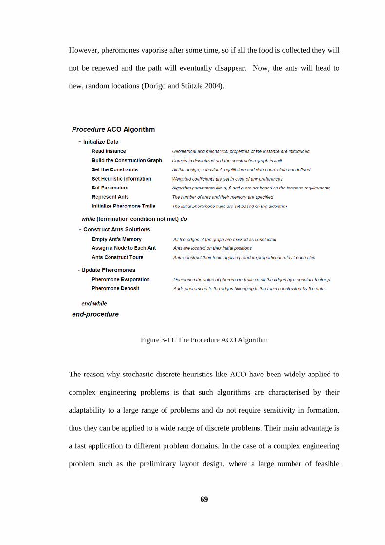
69
However, pheromones vaporise after some time, so if all the food is collected they will
not be renewed and the path will eventually disappear. Now, the ants will head to
new, random locations (Dorigo and Stützle 2004).
Figure 3-11. The Procedure ACO Algorithm
The reason why stochastic discrete heuristics like ACO have been widely applied to
complex engineering problems is that such algorithms are characterised by their
adaptability to a large range of problems and do not require sensitivity in formation,
thus they can be applied to a wide range of discrete problems. Their main advantage is
a fast application to different problem domains. In the case of a complex engineering
problem such as the preliminary layout design, where a large number of feasible
70
options must be examined during the design process, the structure of the problem is
often not known.
Regardless of the number and types of objectives, the size of the problem and the
number of variables in layout optimisation problems, one can use stochastic heuristics
such as ACO, to search for the optimum in a large search space. Such methods can
also provide designers with multiple global solutions instead of an absolute global
solution. Such ability gives the designer the opportunity to have a set of near global
optimum solutions that can be used for different situations where the other ones might
not be valid or suitable. This is why a rather large number of stochastic metaheuristics
is applied for solving a variety of layout design based problems of large sizes (Kaveh
and Shojaee 2007; Kaveh et al. 2008; Kaveh and Sharafi 2008a; b; 2009; Kaveh and
Talatahari 2010).
ACO algorithms have shown to be very successful at obtaining good solutions,
especially for a variety of NP-hard optimisation problems such as knapsack problems
(Dorigo and Stützle 2004; Dorigo 2006; Dorigo et al. 2008). These methods have the
power to sample and find areas of good performance in the highly complex, multi-
dimensional search spaces that typically occur in conceptual design. However, the
effectiveness and convergence to optimal values seem to be the realistic causes of the
broad application of such metaheuristics, rather than the theorem that supports the
methods.
As a non-traditional optimisation tool, the first ACO algorithm was the Ant System
(AS), developed by Dorigo et al. in 1991 (Dorigo and Stützle 2004), which has
successfully been applied to many combinatorial optimisation problems. Various types
of ant-based algorithms have found vast implementations in civil engineering and
71
structural optimisation (Christodoulou 2010; Lee 2012; Sharafi et al. 2012c). . Camp
et al. (2005) proposed an Ant based algorithm for the design of steel frames. Kaveh et
al. (2008) presented an ACO algorithm for structural topology optimisation. Kaveh
and Sharafi (2008a; b; 2009) applied ACO for some graph theory based problems in
structural optimisation.
The two main phases of AS algorithms constitute the ants‘ solution construction and
the pheromone update. In AS a good heuristic to initialise the pheromone trails is to
set them to a value slightly higher than the expected amount of pheromone deposited
by the ants in one iteration. A rough estimate of the value can be obtained by setting
nn
ij Cmji / ),( 0 , where m is the number of ants, and Cnn
is the length or cost
of a tour generated by the nearest neighbor heuristic. The reason for this choice is that
if the initial pheromone values are too low, then the search will be quickly biased by
the first tour generated by the ants, which in general leads to an exploration of inferior
zones of search space. On the other hand, if the initial pheromone values are too high,
then many iterations will be lost waiting until the pheromone evaporates enough
pheromone values, so that pheromone added by ants can start to bias the search.
After defining the construction graph and the constraints, and defining the magnitudes
of the pheromone trails and heuristic information for the problem, the ants start
making the trails. In AS, artificial ants concurrently build a tour. Initially, ants are put
on randomly chosen nodes. At each construction step, Ant k applies a probabilistic
action choice rule known as the random proportional rule, to decide which node to
visit next. In particular, the probability that the Ant k currently on Node i chooses to
go to Node j is

72
if 0
if
k
i
k
i
Nl
ilil
ijij
k
ij
Nj
Njp
ki
(3.14)
This relationship forms the basis of the AS algorithm and shows that if Ant k is
positioned on Node i, it will move to the next Node j with the probability of k
ijp . In
this relationship ij is the pheromone trail and
ij is a heuristic value depending on the
problem conditions. Here and β are two parameters which determine the relative
influence of the pheromone trail and the heuristic information. k
iN is the feasible
neighborhood of the Ant k when being on Node i, that is, the set of nodes that Ant k is
allowed to choose as its next destination. The probabilistic choice of the next node
then works analogously to the roulette wheel selection procedure of evolutionary
computation. The quantity of pheromone trail and heuristic value on the edges
determines the size of the slice on a circular roulette wheel. Obviously, the higher
pheromone or higher heuristic value on the edges increases the possibility of selecting
the corresponding node (Dorigo 2006).
After all the ants have constructed their tours, the pheromone trails are updated. This
update is done by first, lowering the pheromone value on all arcs by a constant factor
(pheromone evaporation), and then adding pheromone on the edges that the ants
have crossed (pheromone depositing). If m ants are used for constructing the solution,
then pheromone updating is implemented by
A(i,j) ρ)τ(1τ ijij (3.15)
73
A(i,j) , Δτττm
1k
k
ijijij (3.16)
where k
ijΔτ is the pheromone added to ij by ant k, and defined as follows:
k
ijΔτ =
otherwise
tobelongs )( edge if /
0
Ti,jC1 kk
(3.17)
The value of Ck can be taken as the cost of the best trail or the best iteration, and T
k is
the set of suitable solutions, depending on the conditions of the problem (Dorigo
Stuzle 2004).
An improvement over AS is rank-based version of AS (ASrank), proposed by
Bullnheimer et al. (1997). In ASrank each ant deposits an amount of pheromone that
decreases with its rank. Ants are sorted by increasing their solution costs. The quantity
of the pheromone that an ant deposits, is weighted according to the rank r of the ant. In
each iteration only the w-1 best-ranked ants are allowed to deposit pheromone,
Bullnheimer et al. (1997). The best iteration gives the strongest feedback, with weight
w and the r-th best ant of the current iteration, contributes to pheromone updating with
the value rr
ij C1 / multiplied by a weight given by w=max{0, w-r}. Thus, the
pheromone update rule is:
bs
ij
w
r
r
ijijij wrw
1
1
)(
(3.18)
In the above relationship, bsbs
ij C1 / is the inverse of the cost of the best selected
iteration. It can be seen that the difference between ASrank and AS lies in the method
for updating the pheromone.
74
The main applications of ACO are for discrete problems, although there are some
modified ACO algorithms than can be applicable for continous forms. This method is
largely being used for solving complicated combinatorial optimisation problems. Due
to the probabilistic nature of such methods, convergence to the global maxima is not
guaranteed.
3.7.1 ACO for Multi-objective Optimisation
A general ACO algorithm consists of three stages, as shown in Fig. 3-11. In the first
stage the evaluation functions, pheromone trails and data were initialised. In the
second stage, ants start constructing the solution using the random proportional rule.
The third stage is to evaluate the solutions and update the pheromone trails according
to their fitness values to help the succeeding ants select a better path. The second and
third stages cycle until all ants have finished constructing their solutions and the
termination criterion is met.
A multi-colony ACO algorithm (Iredi et al. 2001) is used for multi-objective
optimisation problems. There is an independent family of ants for each objective
function, and the ants within each family search for optimal solutions to their assigned
objective function. This search is carried out using a cooperation mechanism, where
any information updated by an ant becomes available for all the other ants within the
same family. Solutions proposed by a family are also transmitted to ants belonging to
the other families, and the recipient ants then modify them to suit their respective
objective functions. When all the families have participated in constructing a solution,
non-dominated solutions receive pheromone for the next iteration (Coello et al. 2007;
Dorigo et al. 2008). This enables several members of the Pareto optimal set to be
found in a single run instead of a series of runs, which is the case for some of the

75
conventional stochastic processes. The computational results suggest that a multi-
colony approach leads to improved performance when compared to using a single
colony with single heuristic information (Dorigo et al. 2006).
Figure 3-12. The Algorithmic Skeleton for Multi-objective ACO
For a multi-objective problem with Q objectives, multiple pheromone information is
defined for each objective and weights are used to aggregate them into a single value
for each family. Each Edge j in a solution Sq for the objective function fq has its own
pheromone matrix 𝜏𝑆𝑗𝑞 and heuristic information matrix 𝜂𝑆𝑗
𝑞 that describes the
desirability of choosing Edge j. Given the construction graph, pheromone and heuristic
information matrices, the probability with which the Ant k chooses Edge j to its partial
solutions is:
𝑝𝑆𝑗𝑘 =
[ (𝜏𝑆𝑞𝑗
𝑞 )𝜆𝑞𝑄𝑞=1 ]𝛼 . [ (𝜂𝑆𝑞𝑗
𝑞 )𝜆𝑞𝑄𝑞=1 ]𝛽
[ (𝜏𝑆𝑞𝑗
𝑞 )𝜆𝑞𝑄𝑞=1 ]𝛼 . [ (𝜂𝑆𝑞𝑗
𝑞 )𝜆𝑞𝑄𝑞=1 ]𝛽 𝑙∈𝑁𝑆
𝑘
(3-19)
where 𝑁𝑆𝑘 is the feasible neighborhood of Ant k, given the current state vector S ={S1,
S2, …, SQ}; 𝛼 and β are two parameters determining the relative influence of the
76
pheromone trail and the heuristic information, and 𝜆𝑞 is the value that weighs the
relative importance of the qth
objective function. Thus, the qth
objective is not
considered when 𝜆𝑞 = 0 and it is the only one considered when 𝜆𝑞 = 1 .
In a multiple ACO algorithm the set of weight vectors that each colony applies in
order to aggregate its multiple pheromone information represents a region in objective
space where the colony focuses its search. For the bi-objective case, as represented by
Eq. (3-20), a single value 𝝀 is enough to define each weight vector {1−𝝀, 𝝀}, as Q = 2.
In this case Eq. (3-20) can be used in lieu of Eq. (3-19) because it shows the
probability with which the Ant k located on Node i to choose Node j.
𝑝𝑖𝑗𝑘 =
[ (𝜏𝑖𝑗1 )(1−𝜆) (𝜏𝑖𝑗
2 )𝜆]𝛼 . [ (𝜂𝑖𝑗1 )(1−𝜆) (𝜂𝑖𝑗
2 )𝜆]𝛽
[ (𝜏𝑖𝑗1 )(1−𝜆) (𝜏𝑖𝑗
2 )𝜆]𝛼 . [ (𝜂𝑖𝑗1 )(1−𝜆) (𝜂𝑖𝑗
2 )𝜆]𝛽 𝑙∈𝑁𝑖
𝑘
(3-20)
In multi-objective problems, as in single objective ones, the iteration-best or best-so-
far strategy can be used for pheromone updates by taking the best solutions from a
candidate set, including all the solutions found in the current iteration, or since the
start of the algorithm. In this case the straightforward criterion is the Pareto optimality
and thus the best solutions for the candidate set are those that are non-dominated, or in
other words, those solutions that belong to the Pareto set. As each objective defines the
solution components in a different way, the selected solutions update each pheromone
matrix differently because each solution component has its own meaning for every
pheromone matrix (Iredi et al. 2001). In this strategy only the best solutions with
respect to each objective are selected to update the pheromone information. Then, each
pheromone matrix, associated with each objective, is updated by the solution with the
best objective value for the corresponding objective. Therefore, the minimum number

77
of ants allowed to update the pheromone information in a colony is equal to the
number of objectives. Since an ant cannot update the pheromone information of more
than one colony, each pheromone matrix focuses on one objective, thus the
aggregation of all of them by means of a weight vector regulates the relative
importance of each objective.
In the pheromone updating stage of multi-objective ACO, some special care must be
taken to guarantee an acceptable convergence. For pheromone depositing, the only
restriction is that the cost of the total solution cannot be used for this purpose because
the values of different objective functions are not comparable and the amount of
deposited pheromone must be ensured to be independent for each family, otherwise
some objectives are considered implicitly more important than the others. With regard
to the pheromone evaporation procedure, any method can be used although efficient
techniques would of course be preferred (Iredi et al. 2001; Dorigo 2006; Dorigo et al.
2008).
3.8 Summary
In the many optimum design cases, we looked for a set of design variables selected
from a given list, which assured the optimum of objective function together with the
satisfaction of constraints. That is, the optimum design consists of selecting the best
combination of a finite number of structural elements and available parameters. Such a
combinatorial nature, from the mathematical point of view, gives the optimum design
procedure a discrete nature. Progress in modern metaheuristics, along with rapidly
advancing computer technology, enables designers to deal with the problems of large
sizes. Combinatorial optimisation problems arise everywhere and certainly in all areas
of technology and industrial management. In proposals for their solution, most
78
combinatorial optimisation problems can be formulated naturally in terms of graphs
and (integer) linear programs. Over the last few decades combinatorial optimisation
and graph theory have experienced a particularly fast development, as has the whole
field of combinatorics in general.
The shortest path and Knapsack problems are two combinatorial problems on which a
large number of real life optimization problems can be formulated. There are hundreds
of applications in applied mathematics, engineering and management for these two
problems. The shortest path and Knapsack problems are both NP hard problems that
are being widely dealt with by randomised search metaheuristics in the literature.
In order to describe the column layouts of buildings with an orthogonal floor plan, it is
practical to divide the floor plan by rectangular areas that are represented by four
columns at each corner such that a rectilinear pattern is formed by a number of
rectangular sub-areas. Each rectangle is treated as an item selected from the set of
rectangles whose dimensions meet the related geometric constraints. Assuming there
is a set of rectangles of various lengths and widths, which meet the geometric
requirements, such as the maximum and minimum length spans. These rectangles
represent the relative location of four columns on their corners and the floor (or slab)
surrounded by them. Rectangles are used to form a rectilinear shape of area A. The
problem changes to select a set of rectangles of total area A and an appropriate
arrangement of them that maximises the profit (objective function) and meets the
constraints.
Therefore, the problem of optimising the layout of a framed building turns to
unbounded multi-constraint multiple knapsack problems. Profit can be defined as the
inverse of cost and/or the inverse of lateral displacement, or any other objectives
79
depending on the problem. Depending on the desired geometric layout, some special
cases can be considered to simplify the application of the method, but each case can be
treated as a certain type of knapsack problem.
For the problem of the column layout design of frames with rectangular shapes, the
problem can be treated as a shortest path problem by discretising the search space and
forming a directed graph that represents the construction graph in the ACO algorithm
as well. Calculating the relevant cost for each feasible solution, the path with the
minimum cost, or shortest path, is the solution for the column layout problem.
Metaheuristics can be an efficient way of producing acceptable solutions to a complex
problem by trial and error in a reasonably practical time. The complexity of the
problem makes it impossible to search every possible solution or combination, so the
aim is to find a good feasible solution in an acceptable timescale.
Ant Colony Optimisation is a non-traditional random search metaheuristic based on
the metaphor of ants seeking food. In order to do so, an ant will leave the anthill and
begin to wander in a random direction. ACO has been widely used for solutions to a
variety of combinatorial optimisations.
80
4 Optimum Column Layout Design for Continuous Beams
4.1 Introduction
This chapter presents a computer aided design method for conceptual geometric layout
optimisation of multi-span reinforced concrete (RC) beams for any type of static or
dynamic response. A key feature of the chapter is the development of a new cost
optimisation method for geometric layout problems that take both cost parameters and
dynamic responses into account to achieve an optimum design along with acceptable
dynamic performance of reinforced concrete (RC) beams. This method takes
advantage of a new optimisation formulation that simplifies the preliminary layout
design computations. First, a new objective function is proposed and formulated as an
alternative to traditional cost functions for reinforced concrete beams. The ability to be
easily used in layout optimisation problems gives the new cost function a distinct
advantage over its alternatives because the problem is then modelled on the shortest
path problem. Using the proposed cost function, an Ant Colony Optimization (ACO)
based algorithm was proposed to determine the optimal lengths of multi-span beams in
81
order to minimise their cost. Examples are included to illustrate the performance of the
new methodology.
In the next section a preliminary geometric design method is presented to determine
the optimum spans of a vibrating continuous beam for controlling dynamic response,
while a given set of design conditions, including the cost of the material and the
loading and support conditions, are given. That is, the optimisation problem was
formulated that considers the cost elements and the dynamic responses. For this
purpose a methodology that links the cross sectional action of the RC beam to the cost
parameters (Sharafi et al. 2012c) was used, and then, based on the proposed objective
function and relevant constraints, an Ant Colony Optimization (ACO) algorithm was
presented to solve the proposed optimisation problem. In order to verify the suitability
of this methodology and illustrate the performance of the algorithm, solved examples
are presented.
4.2 Optimum Design for Static Loading
When designing concrete structures the designer is faced with four classes of design
variables. The first class is material design variables such as the type of concrete to be
used, the second class is topological design variables such as the number of spans in a
frame, and the third class is geometric layout variables such as the length of spans in a
continuous beam; and finally, cross section design variables such as the dimensions of
a concrete section (Kirsh 1981). On most occasions in the optimisation process, the
designer is not free to set the pre-assigned parameters and design variables, and the
existing circumstances may dictate to the designer what to do. Nevertheless, by
exploiting experience one may shift from one set of variables to another that causes a
new definition for the objective function (cost function in this case). Moreover, any
82
changes in choosing the design variables may lead to changes in constraints and even
vary their nature from design variables to behavioural ones, and vice versa. In other
words, depending on the nature of the optimisation problem, the process of achieving
an optimum feasible solution may be much quicker by shifting from one design space
to another, and by changing the design variables into space dimensions.
Selecting the cost function can be considered the most important decision in the entire
optimal design process, and therefore it is essential to introduce a cost function that
represents the most influential cost components and more importantly, one that is
applicable for a variety of similar optimisation problems. Furthermore, it must be
capable of matching the explicit constraints of structures, which are often given by
formulae in design codes.
A cost function generally includes the cost of materials, transportation, fabrication and
even maintenance costs, in addition to repair and insurance costs, which can be
presented by a weighted sum of a number of properties. The effect of these factors in
the optimal cost can be imposed on the weighted coefficients of the cost function. In
concrete structures at least three different cost items should be considered in
optimisation: the cost of concrete, steel, and the formwork. So, the general cost
function for a reinforced concrete beam can be expressed in the following form:
C =Cc+Cs+Cf (4-1)
where C, Cc ,Cs and Cf are the total cost, cost of concrete, cost of steel, and cost of the
formwork, respectively. Obviously, for pre-stressed and fibred concrete sections the
relevant costs for these two items are added to the total cost. Considering the unit costs
per parameter and the fact that the unit costs of longitudinal reinforcement steel
usually differs from shear steel; Eq. (7-1) can be written as
83
C =cc Ac + csl Asl + csv Asv + cf Pf (4-2)
Where cc, csl, csv and cf are the unit costs of concrete, longitudinal steel, shear steel and
formwork respectively and Ac, Asl, Asv and Pf are their corresponding quantities. In unit
costs all the relevant costs, such as material, labour, transportation, fabrication and
maintenace etc. can be taken into account. In most published optimisation studies
(Adeli and Sarma 2006), the costs are calculated for a member such as a beam, and
coefficients and quantities are presented based on members or the unit length of each
member in Eq. (4-2). If such a classic cost function for a beam optimisation problem is
used, some or all of the parameters Ac, Asl, Asv and Pf are considered the design
variables. Then, based on explicit constraints, which are presented in codes and/or
implicit behavior constraints of the problem, the optimum values of the design
variables will be found using optimisation techniques. In other words, most existing
cost optimisation functions only deal with cross sectional variables.
In the case of a multi-objective optimisation of structures, including a combination of
material, geometrical layout, topological, and cross sectional design variables, using
the currently available formulation leads to a significant number of design variables
and constraints because each of the stated conditions might require a complicated trial
and error procedure. In fact, the design variables of this kind, even in the traditional
methods of design, require sound engineering judgment to be chosen, and it can be
extremely time consuming to determine the solution for each section of each member.
Therefore, unless alternative design variables are selected for the cost function, a
multi-objective optimisation procedure might be too unwieldy in these cases.
84
In the problem of the preliminary layout optimisation of multi-span RC beams,
parameters such as the cross sectional area, perimeter of the concrete section or the
area of reinforcement steel, are not truly suitable as design variables because they were
not obtained from an explicit mathematical procedure. These parameters are mainly
calculated using suggested relationships in design codes which do not uniquely
provide the exact values for these parameters. Furthermore, the first step in
determining these parameters is to complete the structural analysis procedure and then
use the structural analysis outputs such as forces and moments together with the
design code requirements to determine the cross sectional characteristics of the
concrete beam. In such a case, each step of the layout optimisation, as in an iterative
procedure, includes both analysis and design processes, and besides the classic cross
sectional variables, the layout of a structure and consequently the outputs of structural
analysis would be variables of the problem. Therefore, designers must repeat the
design procedure to achieve the optimal cross sectional variables that are usually
functions of other analytical outputs.
Consider Eq. (4-3) as a potential alternative cost function to Eq. (4-2) in an arbitrary
beam cross section.
C =c1𝑀𝑢++ c2 𝑀𝑢
−+ c3 Vu (4-3)
where 𝑀𝑢+ and 𝑀𝑢
− are the positive and negative bending moment capacities and Vu
is the shear capacity of the section. If an appropriate set of {c1, c2, c3} could be found
such that Eq. (4-3) represents the cost of the section, the design variables would shift
from Ac, Asl, Asv and Pf to 𝑀𝑢+, 𝑀𝑢
− and Vu. In fact, due to the relationship between the
capacity factors of the section and structural analysis outputs in the design codes the
85
aim of using cost functions such as Eq. (4-3) is to use structural analysis outputs
instead of structural design factors.
Using structural analysis outputs as design variables, say the internal action effects of
a beam, has some advantages over using structural design outcomes such as the cross
sectional characteristics of a beam. Firstly, the design action effects of each section
can be easily obtained from structural analysis and in an iterative mathematical
procedure, re-analysing a structure is considerably less time consuming and more
precise than re-designing the structure. If Eq. (4-2) is used to find the optimum layout
of a large structure with respect to the cost elements, the optimisation tool needs to
deal with structural analysis and structural design in each step in order to move
towards an optimum solution. Besides, in the process of obtaining Ac, Asl, Asv and Pf, in
the first step, one needs to have access to the relevant 𝑀𝑢+, 𝑀𝑢
− and Vu. Therefore,
using 𝑀𝑢+, 𝑀𝑢
− and Vu as optimisation variables seems to be a shortcut in finding the
optimum cost in the layout optimisation of multi-span beams.
Moreover, in Eq. (4-3) the cost function is considered in a section rather than a
member. Such ability is an advantage because it enables the designer to select a
number of sections for each member and control the cost in the entire structure, so
there is no necessity to conduct the optimisation process over the entire member. Since
the cross sectional characteristics of a member, say a RC beam, such as Ac, Asl, Asv and
Pf varies along the member, in order to come up with an accurate cost function for a
member, one needs to have a clear idea about the probable distribution of bending
moments and shear forces. Such a requirement makes the formulation extremely
complicated and sometimes impractical for some multi-objective problems.
86
The rest of this chapter describes how to find an appropriate set of coefficients that
make Eq. (4-3) a viable alternative to Eq. (4-2) for optimising the layout of reinforced
concrete continuous beams. Using the proposed cost function, a method to find the
optimum lengths of spans in a multi-span beam in order to minimise the cost is
formulated.
4.2.1 Mathematical formulation
In formulating the cost optimisation of a beam and the relevant constraints, the
Australian design standard for reinforced concrete structures, AS-3600 (2009) was
used since it is based on limit states design method of concrete structures. The
evaluation of the area of steel reinforcement and the area of concrete section are based
on the strength limit states of the section that can occur in either concrete or steel.
Consider an arbitrary section of a rectangular reinforced concrete beam, as shown in
Fig. 4-1. The dimensions of the section are b and h, the areas of tension and
compression reinforcement steel are Ast, Asc respectively, and the area of shear
reinforcement steel in a unit length of beam is Asv/s, where Asv is the area of shear
shear reinforcement (stirrups), and s is the spacing of the stirrups along the member.
The capacity or the ultimate strength of the section in negative and positive flexure
and shear are 𝑀𝑢−, 𝑀𝑢
+ and Vu respectively, which can be obtained from Eq. (4-4)
through Eq. (4-6) in a balanced section in which both tension and compression steel
yield.
𝑀𝑢− ≅ Asc fyl d(1- 0.5γku) (4-4)
𝑀𝑢+ ≅ Asc fyl d(1- 0.5γku) + (Ast -Asc) fyl (d - a/2) (4-5)
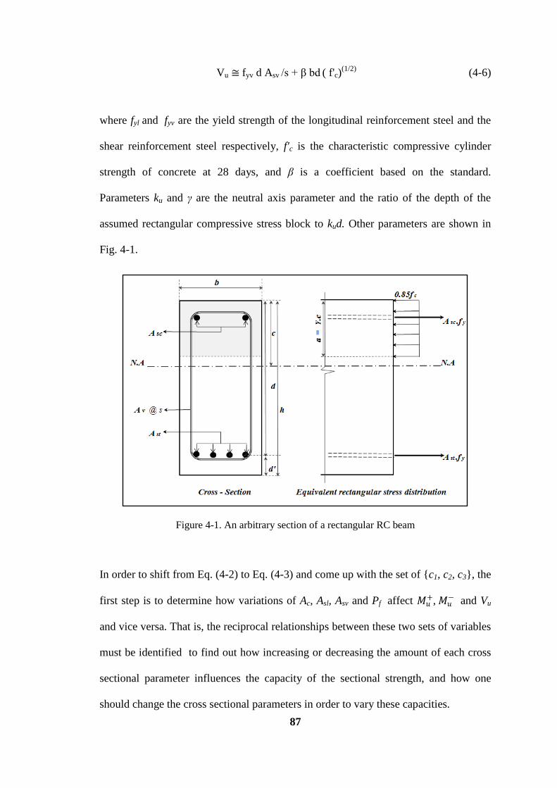
87
Vu ≅ fyv d Asv /s + β bd ( f'c)
(1/2) (4-6)
where fyl and fyv are the yield strength of the longitudinal reinforcement steel and the
shear reinforcement steel respectively, f'c is the characteristic compressive cylinder
strength of concrete at 28 days, and β is a coefficient based on the standard.
Parameters ku and γ are the neutral axis parameter and the ratio of the depth of the
assumed rectangular compressive stress block to kud. Other parameters are shown in
Fig. 4-1.
Figure 4-1. An arbitrary section of a rectangular RC beam
In order to shift from Eq. (4-2) to Eq. (4-3) and come up with the set of {c1, c2, c3}, the
first step is to determine how variations of Ac, Asl, Asv and Pf affect 𝑀𝑢+, 𝑀𝑢
− and Vu
and vice versa. That is, the reciprocal relationships between these two sets of variables
must be identified to find out how increasing or decreasing the amount of each cross
sectional parameter influences the capacity of the sectional strength, and how one
should change the cross sectional parameters in order to vary these capacities.
88
As stated above, given the unit costs cc, csl, csv and cf , the cost function can be defined
using Eq. (4-2) for each section. If any of the cross sectional parameters Ac, Asl, Asv or
Pf changes, the cost function varies in a section as follows
ΔC =cc ΔAc + csl ΔAsl + csv ΔAsv + cf ΔPf (4-7)
On the other hand, using Eq. (4-3) variations in section capacities would change the
cost function as follows:
ΔC = c1Δ𝑀𝑢++ c2 Δ𝑀𝑢
−+ c3 ΔVu (4-8)
Eqs. (4-7) and (4-8) show the contribution of each factor to cost changes and
sensitivity of the cost to each term. For example, changing a unit of Ac causes a change
of cc units in cost. Therefore, if the effect of variations of Ac, Asl, Asv and Pf on
variations of 𝑀𝑢+, 𝑀𝑢
− and Vu are determined, the contribution of each section capacity
to cost changes, that is the set of {c1, c2, c3}, can be found out.
In order to simplify the calculations, two assumptions were made. First, since we
intended the section to remain in a balanced condition, any changes for compression
steel were considered equal to those of tension steel.
ΔAst =ΔAsc = ΔAsl (4-9)
This means, in case of the layout optimisation of multi-span beams where the aim is to
find the optimum length spans, any variations in the quantities of steel s for
compression and tension in a balanced section can be considered equal in each step of
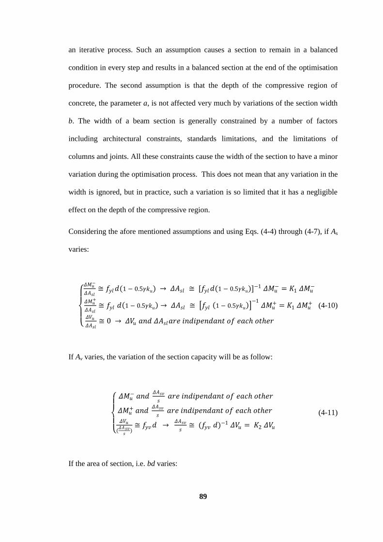
89
an iterative process. Such an assumption causes a section to remain in a balanced
condition in every step and results in a balanced section at the end of the optimisation
procedure. The second assumption is that the depth of the compressive region of
concrete, the parameter a, is not affected very much by variations of the section width
b. The width of a beam section is generally constrained by a number of factors
including architectural constraints, standards limitations, and the limitations of
columns and joints. All these constraints cause the width of the section to have a minor
variation during the optimisation process. This does not mean that any variation in the
width is ignored, but in practice, such a variation is so limited that it has a negligible
effect on the depth of the compressive region.
Considering the afore mentioned assumptions and using Eqs. (4-4) through (4-7), if As
varies:
𝛥𝑀𝑢−
𝛥𝐴𝑠𝑙≅ 𝑓𝑦𝑙 𝑑(1 − 0.5𝛾𝑘𝑢) → 𝛥𝐴𝑠𝑙 ≅ [𝑓𝑦𝑙 𝑑(1 − 0.5𝛾𝑘𝑢)]−1 𝛥𝑀𝑢
− = 𝐾1 𝛥𝑀𝑢−
𝛥𝑀𝑢+
𝛥𝐴𝑠𝑙≅ 𝑓𝑦𝑙 𝑑 1 − 0.5𝛾𝑘𝑢 → 𝛥𝐴𝑠𝑙 ≅ 𝑓𝑦𝑙 1 − 0.5𝛾𝑘𝑢
−1 𝛥𝑀𝑢
+ = 𝐾1 𝛥𝑀𝑢+
𝛥𝑉𝑢
𝛥𝐴𝑠𝑙≅ 0 → 𝛥𝑉𝑢 𝑎𝑛𝑑 𝛥𝐴𝑠𝑙𝑎𝑟𝑒 𝑖𝑛𝑑𝑖𝑝𝑒𝑛𝑑𝑎𝑛𝑡 𝑜𝑓 𝑒𝑎𝑐 𝑜𝑡𝑒𝑟
(4-10)
If Av varies, the variation of the section capacity will be as follow:
𝛥𝑀𝑢
− 𝑎𝑛𝑑 𝛥𝐴𝑠𝑣
𝑠 𝑎𝑟𝑒 𝑖𝑛𝑑𝑖𝑝𝑒𝑛𝑑𝑎𝑛𝑡 𝑜𝑓 𝑒𝑎𝑐 𝑜𝑡𝑒𝑟
𝛥𝑀𝑢+ 𝑎𝑛𝑑
𝛥𝐴𝑠𝑣
𝑠 𝑎𝑟𝑒 𝑖𝑛𝑑𝑖𝑝𝑒𝑛𝑑𝑎𝑛𝑡 𝑜𝑓 𝑒𝑎𝑐 𝑜𝑡𝑒𝑟
𝛥𝑉𝑢
(𝛥𝐴𝑠𝑣
𝑠)≅ 𝑓𝑦𝑣𝑑 →
𝛥𝐴𝑠𝑣
𝑠≅ (𝑓𝑦𝑣 𝑑)−1 𝛥𝑉𝑢 = 𝐾2 𝛥𝑉𝑢
(4-11)
If the area of section, i.e. bd varies:

90
ΔAc = Δ(bd) =b Δd + d Δb + Δb Δd (4-12)
𝑀𝑢− is not a function of b and based on the second assumption we made, the
dependence of M+
u on changes of b is neglected. Moreover, the first term of Vu is not
dependent on b as well. So, the variations of the section capacities due to variation of
section area are as follows:
𝛥𝑀𝑢 𝑏
∆𝐴𝑐 𝑏 =
𝛥𝑀𝑢 𝑏
𝛥 𝑏𝑑 ≅
𝛥𝑀𝑢 𝑏
𝑏 𝛥𝑑 (4-13)
𝛥𝑀𝑢−
𝛥(𝑏𝑑)≅
𝑓𝑦𝑙𝐴𝑠𝑐
𝑏 1 − 0.5𝛾𝑘𝑢 → 𝛥 𝑏𝑑 ≅ 𝑓
𝑦𝑙
𝐴𝑠𝑐
𝑏 1 − 0.5𝛾𝑘𝑢
−1
𝛥𝑀𝑢− = 𝐾3 𝛥𝑀𝑢
−
𝛥𝑀𝑢+
𝛥(𝑏𝑑)≅
𝑓𝑦𝑙
𝑏(𝐴𝑠𝑡 − 0.5𝛾𝑘𝑢𝐴𝑠𝑐) → 𝛥 𝑏𝑑 ≅
𝑓𝑦𝑙
𝑏(𝐴𝑠𝑡 − 0.5𝛾𝑘𝑢𝐴𝑠𝑐)
−1
𝛥𝑀𝑢+ = 𝐾4 𝛥𝑀𝑢
+
𝛥𝑉𝑢
𝛥(𝑏𝑑)≅
𝑓𝑦𝑣𝐴𝑠𝑣
𝑏𝑠+ 𝛽(𝑓′
𝑐)
1/2 → 𝛥(𝑏𝑑) ≅ [
𝑓𝑦𝑣𝐴𝑠𝑣
𝑏𝑠+ 𝛽(𝑓′
𝑐)
1/2]−1
𝛥𝑉𝑢 = 𝐾5 𝛥𝑉𝑢
(4-14)
The variation of the perimeter of a rectangular section, which determines the variation
of the formwork, affects the section capacity as follows:
𝛥𝑃𝑓 = ∆𝑏 + 2∆𝑑 (4-15)
𝛥𝑀𝑢−
∆𝑏+2∆𝑑≅ 0.5𝑓𝑦𝑙𝐴𝑠𝑐 1 − 0.5𝛾𝑘𝑢 → 𝛥𝑃𝑓 ≅ 2 𝑓𝑦𝑙𝐴𝑠𝑐 1 − 0.5𝛾𝑘𝑢
−1 𝛥𝑀𝑢
− = 𝐾6 𝛥𝑀𝑢−
𝛥𝑀𝑢+
∆𝑏+2∆𝑑≅ 0.5𝑓𝑦𝑙 (𝐴𝑠𝑡 − 0.5𝛾𝑘𝑢𝐴𝑠𝑐 ) → 𝛥𝑃𝑓 ≅ 2 𝑓𝑦𝑙 (𝐴𝑠𝑡 − 0.5𝛾𝑘𝑢𝐴𝑠𝑐 )
−1 𝛥𝑀𝑢
+ = 𝐾7 𝛥𝑀𝑢+
𝛥𝑉𝑢
∆𝑏+2∆𝑑≅
2𝑓𝑦𝑙 𝐴𝑠𝑣
𝑠+ 𝛽𝑏 (𝑓 ′
𝑐)1/2+
1
𝛽𝑑 (𝑓 ′𝑐)1/2 → 𝛥𝑃𝑓 ≅
2
𝑓𝑦𝑣 𝐴𝑠𝑣
𝑠+ 𝛽𝑏 𝑓 ′
𝑐 12
+1
𝛽𝑑 𝑓 ′𝑐
12
𝛥𝑉𝑢 = 𝐾8 𝛥𝑉𝑢
(4-16)
Multiplying both sides of Eqs. (4-10) by csl /2, Eqs. (4-11) by csv , Eqs. (4-14) by cc /3
and Eqs. (4-16) by cf /3, and adding them up will result in:
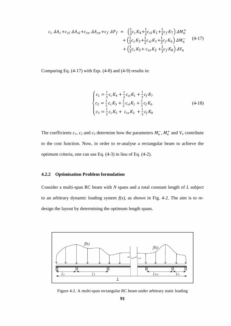
91
𝑐𝑐 𝛥𝐴𝑐+𝑐𝑠𝑙 𝛥𝐴𝑠𝑙 +𝑐𝑠𝑣 𝛥𝐴𝑠𝑣+𝑐𝑓 𝛥𝑃𝑓 = 1
3𝑐𝑐𝐾4+
1
2𝑐𝑠𝑙𝐾1+
1
3𝑐𝑓𝐾7 𝛥𝑀𝑢
+
+
1
3𝑐𝑐𝐾3+
1
2𝑐𝑠𝑙𝐾1+
1
3𝑐𝑓𝐾6 𝛥𝑀𝑢
−
+ 1
3𝑐𝑐𝐾5+ 𝑐𝑠𝑣𝐾2 +
1
3𝑐𝑓𝐾8 𝛥𝑉𝑢
(4-17)
Comparing Eq. (4-17) with Eqs. (4-8) and (4-9) results in:
𝑐1 =
1
3𝑐𝑐𝐾4 +
1
2𝑐𝑠𝑙𝐾1 +
1
3𝑐𝑓𝐾7
𝑐2 =1
3𝑐𝑐𝐾3 +
1
2𝑐𝑠𝑙𝐾1 +
1
3𝑐𝑓𝐾6
𝑐3 =1
3𝑐𝑐𝐾5 + 𝑐𝑠𝑣𝐾2 +
1
3𝑐𝑓𝐾8
(4-18)
The coefficients c1, c2 and c3 determine how the parameters 𝑀𝑢−, 𝑀𝑢
+ and Vu contribute
to the cost function. Now, in order to re-analyse a rectangular beam to achieve the
optimum criteria, one can use Eq. (4-3) in lieu of Eq. (4-2).
4.2.2 Optimisation Problem formulation
Consider a multi-span RC beam with N spans and a total constant length of L subject
to an arbitrary dynamic loading system f(x), as shown in Fig. 4-2. The aim is to re-
design the layout by determining the optimum length spans.
Figure 4-2. A multi-span rectangular RC beam under arbitrary static loading

92
For this purpose the cost will be the sum of the cost functions of all sections selected
in the structure.
𝐶𝑡 = 𝐶𝑖𝑁𝑆𝑖=1 = (𝑐1𝑖𝑀𝑢𝑖
+𝑁𝑆𝑖=1 + 𝑐2𝑖𝑀𝑢𝑖
_ + 𝑐3𝑖𝑉𝑢𝑖 ) (4-19)
where Ct is the total cost of the structure and NS is the number of selected sections to
control the cost.
The strength constraints on each selected section i in the structure under a load case
may be written as
∅𝑓 𝑀𝑢𝑖+ ≥ 𝑀𝑖
∗+
∅𝑓 𝑀𝑢𝑖− ≥ 𝑀𝑖
∗−
∅𝑠 𝑉𝑢𝑖 ≥ 𝑉𝑖∗
for i={1,2,…NS} (4-20)
where 𝑀𝑖∗+
, 𝑀𝑖∗−
and 𝑉𝑖∗ are positive and negative flexure and shear action effects
of section i. ∅𝑓 and ∅𝑠 are the strength reduction factors in flexure and shear
respectively. The serviceability requirements limit the maximum deflection umax on the
entire member to Δmax under the serviceability load case. So for all sections:
umax i ≤ Δmax i for i={1,2,…NS} (4-21)
Other constraints for durability, fire resistance, minimum cover and minimum flexural
strength, can be easily added to the problem as well, based on the relevant design
codes.
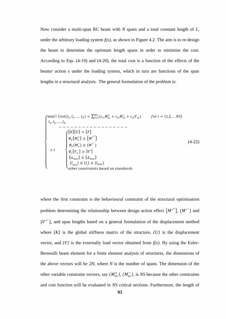
93
Now consider a multi-span RC beam with N spans and a total constant length of L,
under the arbitrary loading system f(x), as shown in Figure 4.2. The aim is to re-design
the beam to determine the optimum length spans in order to minimise the cost.
According to Eqs. (4-19) and (4-20), the total cost is a function of the effects of the
beams' action s under the loading system, which in turn are functions of the span
lengths in a structural analysis. The general formulation of the problem is:
min 𝐶𝑜𝑠𝑡(𝑙1, 𝑙2, … , 𝑙𝑁) = (𝑐1𝑖𝑀𝑢𝑖+𝑁𝑆
𝑖=1 + 𝑐2𝑖𝑀𝑢𝑖− + 𝑐3𝑖𝑉𝑢𝑖) 𝑓𝑜𝑟 𝑖 = {1,2, … 𝑁𝑆}
𝑙1, 𝑙2, … , 𝑙𝑁
− − − − − − − − − − − − − − − − − −
𝑠. 𝑡
𝐾 𝑈 = 𝐹
∅𝑓 𝑀𝑢+ ≥ 𝑀∗+
∅𝑓{𝑀𝑢−} ≥ {𝑀∗−
}
∅𝑠 𝑉𝑢 ≥ 𝑉∗
𝑢𝑚𝑎𝑥 ≤ 𝛥𝑚𝑎𝑥
{𝑙𝑚𝑖𝑛
} ≤ {𝑙𝑖} ≤ {𝑙𝑚𝑎𝑥}
𝑜𝑡𝑒𝑟 𝑐𝑜𝑛𝑠𝑡𝑟𝑎𝑖𝑛𝑡𝑠 𝑏𝑎𝑠𝑒𝑑 𝑜𝑛 𝑠𝑡𝑎𝑛𝑑𝑎𝑟𝑑𝑠
(4-22)
where the first constraint is the behavioural constraint of the structural optimisation
problem determining the relationship between design action effect 𝑀∗+ , {𝑀∗−
} and
{𝑉∗−}, and span lengths based on a general formulation of the displacement method
where [K] is the global stiffness matrix of the structure, {U} is the displacement
vector, and {F} is the externally load vector obtained from f(x). By using the Euler-
Bernoulli beam element for a finite element analysis of structures, the dimensions of
the above vectors will be 2N, where N is the number of spans. The dimension of the
other variable constraint vectors, say {𝑀𝑢𝑖+ }, {𝑀𝑢𝑖
− }, is NS because the other constraints
and cost function will be evaluated in NS critical sections. Furthermore, the length of
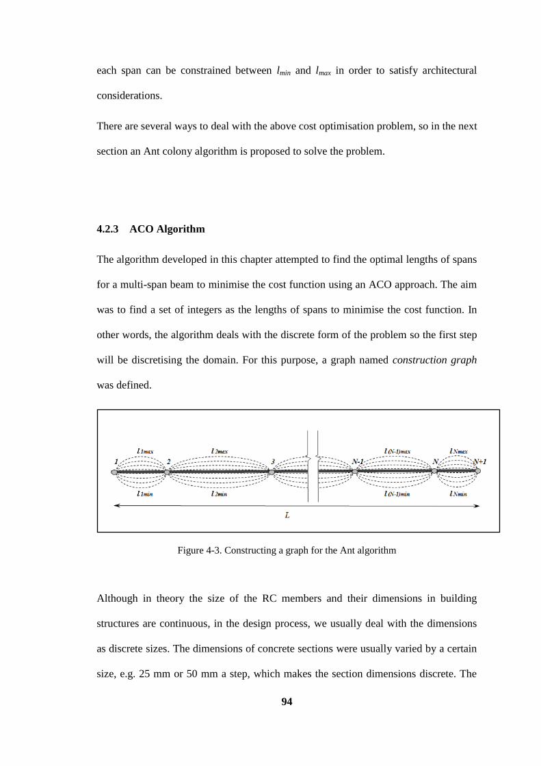
94
each span can be constrained between lmin and lmax in order to satisfy architectural
considerations.
There are several ways to deal with the above cost optimisation problem, so in the next
section an Ant colony algorithm is proposed to solve the problem.
4.2.3 ACO Algorithm
The algorithm developed in this chapter attempted to find the optimal lengths of spans
for a multi-span beam to minimise the cost function using an ACO approach. The aim
was to find a set of integers as the lengths of spans to minimise the cost function. In
other words, the algorithm deals with the discrete form of the problem so the first step
will be discretising the domain. For this purpose, a graph named construction graph
was defined.
Figure 4-3. Constructing a graph for the Ant algorithm
Although in theory the size of the RC members and their dimensions in building
structures are continuous, in the design process, we usually deal with the dimensions
as discrete sizes. The dimensions of concrete sections were usually varied by a certain
size, e.g. 25 mm or 50 mm a step, which makes the section dimensions discrete. The
95
amount of reinforcement was also determined by the number of bars in a RC section.
Therefore, one can define the optimisation problem of RC sections as a discrete
optimisation problem rather than a continuous one.
In order to discretise the domain of answers, assume that the span lengths are bounded
in [lmin, lmax] with intervals (accuracy) equal to ε, then each li rests in the set of {lmin ,
lmin + ε, lmin + 2ε ,…, lmax - ε , lmax}. Obviously, the smaller ε is chosen, the more
accurate results will be obtained and the more running time the algorithm needs. The
number of spans (beam elements) and the number of nodes in the continuous beam is
N and N+1respectively so the construction graph was defined as a graph with N+1
nodes and (lmax - lmin)/ ε *N edges, as shown in Fig 4-3. Each pair of nodes were
connected with (lmax - lmin)/ ε edges, i.e. there are (lmax - lmin)/ ε choices for each Ant on
each node to select another one, for making its trail (solution). It should be pointed out
that, as stated in the definition of constraints and shown in Figure 3, lmax and lmin might
be specified differently for each span, say li max and li min. In this case, the number of
choices for ants on each node might differ from the other ones. Now that the
construction graph is prepared, Ants can start their solution process in three phases
(Kaveh and Sharafi 2008, 2009). The algorithm flowchart is shown in Fig. 4.4
1- The phase of initial data processing and preliminary calculation; In this phase the
primary values are given and the calculations start and data are entered. Artificial Ants
were located on the first and last nodes of the construction graph, i.e. Nodes 1 and
N+1, to construct their solution. The lengths of paths are introduced and parameters
,, and the termination criteria are defined and initial pheromone and heuristic
matrix are organised. Each value (i,j) of pheromone matrix and heuristic matrix shows
the tendency of the Ant located on Node i of the construction graph to choose the edge
j to move towards the next node. Since there are as many as (lmax - lmin)/ ε edges that
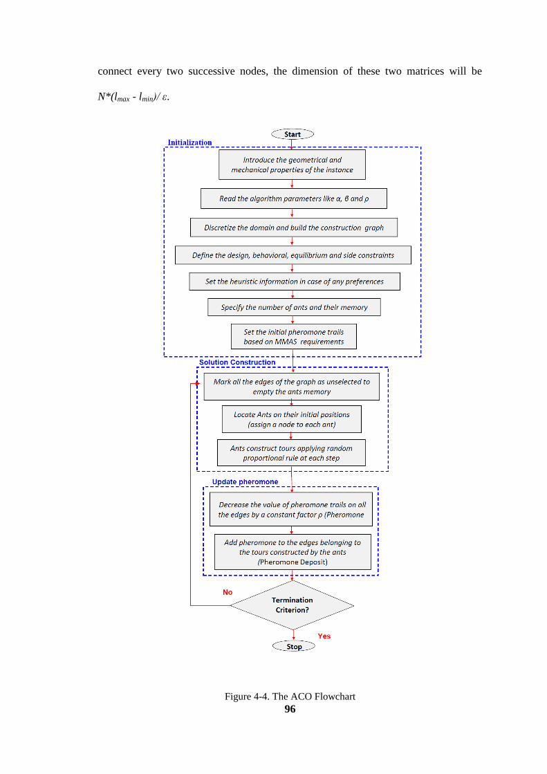
96
connect every two successive nodes, the dimension of these two matrices will be
N*(lmax - lmin)/ ε.
Figure 4-4. The ACO Flowchart
97
For organising the heuristic matrix and initial pheromone matrix, we can make use of
our structural analysis experience. Because the type of supports and other boundary
conditions and constraints, plus any loads, can affect the length of spans, the entries of
heuristic matrix and initial pheromone matrix might be organised based on such
parameters. Technically, the arrays of the heuristic matrix are specified according to
the designers' preferences. In this case for example, if there are any preferences for
certain length spans due to say architectural constraints, higher values that correspond
to those lengths are assigned to the heuristic arrays. Since the heuristic matrix does
not change during the optimisation process, such an assignment will cause the desired
lengths to be more likely to be chosen by ants for the corresponding spans. Then by
choosing appropriate values for α and β the degree of influence of the heuristic values
in comparison with the pheromone trail is determined. Moreover, in order to save
time, some criteria like the symmetry of the beam are considered when the heuristic
matrix is formed. Using such a heuristic matrix or defining the initial pheromone
matrix using the above mentioned structural rules helps the algorithm to converge
sooner. Thus, each value (i,j) of the chosen information matrix obtained by
multiplying the corresponding arrays of heuristic matrix by those of the pheromone
matrix, shows the tendency or desirability of the Ant located on Node i of construction
graph to choose Edge j to move toward Node i+1.
2. The phase of the construction of solution: This phase consists of two segments that
form the basis of the heuristic. In the first segment of this phase, Ants located on the
starting nodes of construction graph, whether Node 1 or Node N+1, begin to construct
their solutions using the random proportional rule of Eq. (3-14).
98
This relationship forms the basis of the AS algorithm and shows that if Ant k is
positioned on Node i, it will move to the next Node j with the probability of ρijk. In this
relationship, τij is the magnitude of pheromone on the trails and ηij is the heuristic
value. α and β are two parameters which determine the relative influence of the
pheromone trail and the heuristic information. Nik is the feasible neighborhood of Ant
k when being at Node i, that is, the set of nodes that Ant k is allowed to choose as its
next destination and hasdecided on, depending on the problem at hand.
In this method the feasible neighborhood k
iN is defined as the edges between Nodes i
and i+1, when the Ant is located at Node i in either route. Then, the Ant leaves its
source Node i{1,2,…,N+1} on the construction graph to its destination node on the
connecting Edges j{1, 2, …, (lmax - lmin)/ ε }, using the random proportional rule,
which is similar to the random roulette wheel rule and quite randomly based on Eq. (3-
14). The probability of Edge j being chosen by Ant on Node i is proportional to the
entry (i, j) of the choice information matrix. The bigger the entry (i,j) of the choice
matrix is, the more probable is Node j to be chosen by Ant i. The Ants continue
constructing their solution and move from one node to another, until they arrive at
Node N+1 which is the end of their trail. The constraint for Ants is that the sum of all
spans must be equal to L. Therefore, two groups of Ants are located on both ends of
the graph, so that every edge has the same overall probability of being chosen by the
Ants.
After the segment of random choice, the values of N lengths and thereby the new
geometrical layout for the beam is obtained. Through structural analytical methods,
and using the behaviour constraints, the effects of the design actions in the identified
sections are determined, and the required strengths for each section are calculated.

99
Based on the strength of the sections, the cost function or the cost of this solution is
obtained.
3. The phase of Updating: This phase consists of updating information and statistics,
and then updating pheromone trails. Using the information obtained in the phase of
constructing the solution, the trail presenting the best cost, up to this stage, is selected
as the best iteration so far, and after which the pheromone trails of the construction
graph are updated. For this reason Ants are allowed to deposit pheromone on the edges
associated with the best iteration so far. The process of updating the pheromone
consists of two segments; the first segment corresponds to pheromone evaporation
according to Eq. (3-15) which is done by first lowering its value on all arcs by a
constant factor ρ (pheromone evaporation):
In this segment the parameter depends on the number of steps defined for the
termination criteria and the initial pheromone and heuristic values. The second
segment is depositing pheromone according to Eq. (3.16), where Δτijk is the
pheromone added to τij by Ant k, and defined according to Eq. (3.17).
The value of Ck is taken as the cost of the best trail or the best iteration and T
k is the set
of suitable solutions. For depositing pheromone the pheromone values on the edges
associated with the best iteration up to now increase, and the Ant deposits an amount
of pheromone equal to 1/cost on the edges of the construction graph associated with
the best iteration so far, and where cost is the value of the cost function obtained from
best iteration.
The above procedure continues until the termination criterion has been satisfied, and
then the optimum spans will be the best solution so far. As seen, in each step a simple
structural analysis is required to calculate the beam actions. By making use of various
100
finite element methods, such a calculation takes a small fraction of a second for each
beam. Using Eq. (4-2) as the objective function would be significantly more time
consuming than using Eq. (4-3). Due to the variation of lengths in each step,
estimating the design variables in each step would be encumbered considerably, apart
from the fact that in each step, the algorithm would iteratively need to deal with the
design formulas. Eq. (4-3) makes the optimisation process more tangible and readily
usable in optimising the cost of large structures.
4.2.4 Numerical Examples
Two examples were presented to demonstrate the efficiency of the proposed
methodology. All the computations were performed on P9700 @2.80 GHz computer
running MATLAB R2009b. In order to ensure that the solution obtained from ACO is
global or near global optimum, several runs were made in parallel. Since each run is
fully independent of the others, the program can be run in parallel so that the total
execution time will be practically the same as that required for a single run. At the end,
a typical convergence history is illustrated for each algorithm using the proposed ACO
algorithm for the examples.
Example 1: consider a three-span beam with its geometrical details, and its live and
dead loads, as shown in Fig. 4-4. The beam supports a 120 mm thick slab inside a
residential building. The material properties and relative cost factors are: f'c=25 MPa,
fyl= fyv =400 MPa, cc=1, csl= csv =66, cf=0.42. The ratio of effective span to the
maximum total deflection should not be less than 250. The aim is to find the optimum
l1, l2, and l3, to minimise the costs.

101
Figure 4-5. Example 1: Three-span beam with uniformly distributed loads
A similar problem given l1 = 7000 mm, l2 =5000 mm, and l3 =4000 mm, was solved
by Kanagasunda and Karihaloo (1991). This design was used as the initial design to
start the optimisation process for the spans. It should be added that every initial design
based on the preliminary judgment of the designer and/or using approximate charts or
formulas, which meets the design code requirements, can be used as the initial design
and as the starting point of the optimisation process. According to their solution for the
seven sections selected from A to G, based on AS3600 (2009), and considering the
above mentioned costs, the primary cost of the structure based on Eq. (4-2) equals
4648 units
It should be noted that the number of selected sections depends entirely on the number
of critical or control ones, and one may choose more sections to achieve much
accurate results. Using Eqs. (4-10), (4-11), (4-14) and (4-16) the values of K1 to K8,
and using Eq. (4-18) the values of c1, c2 and c3 for sections A to G are obtained.
Having the necessary coefficients, the cost function can be defined, based on Eq. (4-
19).
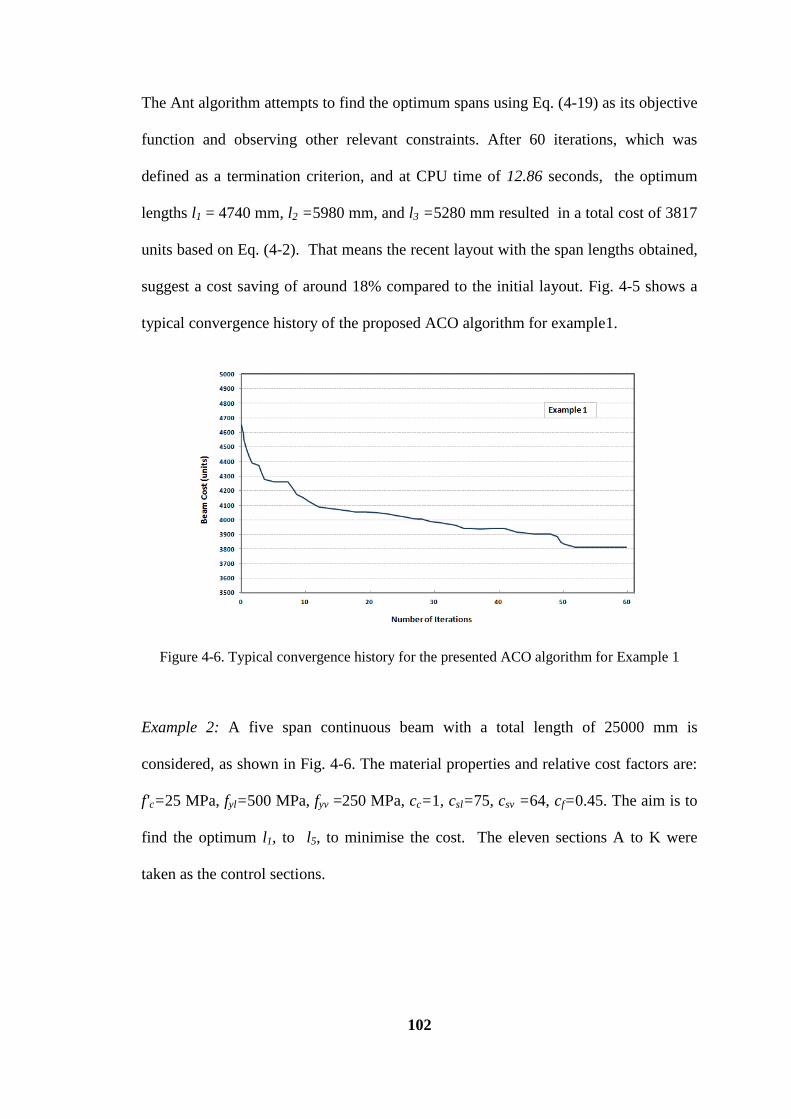
102
The Ant algorithm attempts to find the optimum spans using Eq. (4-19) as its objective
function and observing other relevant constraints. After 60 iterations, which was
defined as a termination criterion, and at CPU time of 12.86 seconds, the optimum
lengths l1 = 4740 mm, l2 =5980 mm, and l3 =5280 mm resulted in a total cost of 3817
units based on Eq. (4-2). That means the recent layout with the span lengths obtained,
suggest a cost saving of around 18% compared to the initial layout. Fig. 4-5 shows a
typical convergence history of the proposed ACO algorithm for example1.
Figure 4-6. Typical convergence history for the presented ACO algorithm for Example 1
Example 2: A five span continuous beam with a total length of 25000 mm is
considered, as shown in Fig. 4-6. The material properties and relative cost factors are:
f'c=25 MPa, fyl=500 MPa, fyv =250 MPa, cc=1, csl=75, csv =64, cf=0.45. The aim is to
find the optimum l1, to l5, to minimise the cost. The eleven sections A to K were
taken as the control sections.
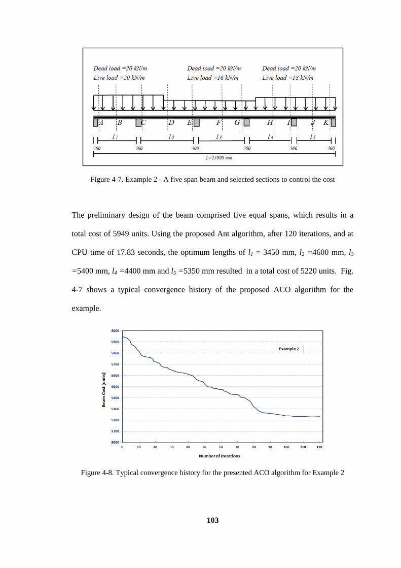
103
Figure 4-7. Example 2 - A five span beam and selected sections to control the cost
The preliminary design of the beam comprised five equal spans, which results in a
total cost of 5949 units. Using the proposed Ant algorithm, after 120 iterations, and at
CPU time of 17.83 seconds, the optimum lengths of l1 = 3450 mm, l2 =4600 mm, l3
=5400 mm, l4 =4400 mm and l5 =5350 mm resulted in a total cost of 5220 units. Fig.
4-7 shows a typical convergence history of the proposed ACO algorithm for the
example.
Figure 4-8. Typical convergence history for the presented ACO algorithm for Example 2
104
4.3 Optimum Design for Dynamic Loading
Structures optimised to a particular load system may not be optimised when subjected
to another load system, so various load cases must be considered when formulating
the optimisation problem. In fact, in a comprehensive computer aided structural
optimisation process, selecting an appropriate preliminary geometric layout design of
structures is very important because it influences all the subsequent stages of the
design procedure. The aim of this computational effort is to determine the preliminary
geometry so that the desired behaviour is achieved at the lowest possible cost. It
focuses on minimising the structural cost subject to constraints on eigen-frequencies,
modal shapes, and the static and dynamic equilibrium.
Improving the vibration characteristics of a structure by changing the structural
topology has long been a subject that has attracted the minds of engineers. One of the
first applications of the layout or topology optimisation methods for the design of
machines and structures subjected to dynamic loads was in eigenvalue optimisation for
free vibrations. One method for optimising the overall stiffness of a structure without
reference to any specific loading is to maximise a linear combination of the first N
vibrational eigenvalues (Pedersen 2000).
When optimising the cost and geometric layout and/or topology of complex structures
under dynamic conditions, a lot of variables that would result in a large computation
time must be considered. As a result, most of the cost optimisation methods developed
for multi-member structures are confined to structures with predefined shapes, and
may not always be applicable to the topological design of large scale problems due to
difficulties in computational cost and convergence properties.
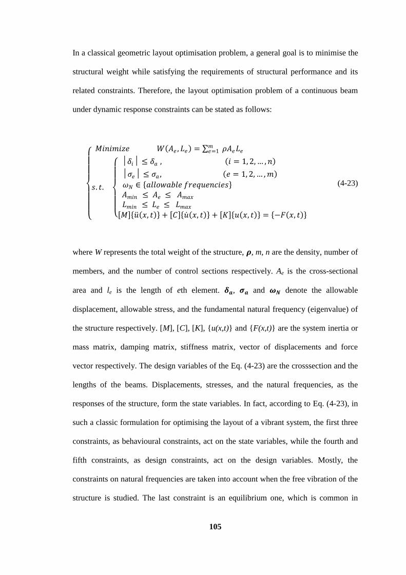
105
In a classical geometric layout optimisation problem, a general goal is to minimise the
structural weight while satisfying the requirements of structural performance and its
related constraints. Therefore, the layout optimisation problem of a continuous beam
under dynamic response constraints can be stated as follows:
𝑀𝑖𝑛𝑖𝑚𝑖𝑧𝑒 𝑊 𝐴𝑒 , 𝐿𝑒 = 𝜌𝐴𝑒𝐿𝑒𝑚𝑒=1
𝑠. 𝑡.
│𝛿𝑖│ ≤ 𝛿𝑎 , 𝑖 = 1, 2, … , 𝑛
│𝜎𝑒│ ≤ 𝜎𝑎 , 𝑒 = 1, 2, … , 𝑚
𝜔𝑁 ∈ 𝑎𝑙𝑙𝑜𝑤𝑎𝑏𝑙𝑒 𝑓𝑟𝑒𝑞𝑢𝑒𝑛𝑐𝑖𝑒𝑠 𝐴𝑚𝑖𝑛 ≤ 𝐴𝑒 ≤ 𝐴𝑚𝑎𝑥 𝐿𝑚𝑖𝑛 ≤ 𝐿𝑒 ≤ 𝐿𝑚𝑎𝑥
𝑀 𝑢 𝑥, 𝑡 + 𝐶 𝑢 𝑥, 𝑡 + 𝐾 𝑢 𝑥, 𝑡 = −𝐹 𝑥, 𝑡
(4-23)
where W represents the total weight of the structure, 𝝆, m, n are the density, number of
members, and the number of control sections respectively. Ae is the cross-sectional
area and le is the length of eth element. 𝜹𝒂, 𝝈𝒂 and 𝝎𝑵 denote the allowable
displacement, allowable stress, and the fundamental natural frequency (eigenvalue) of
the structure respectively. [M], [C], [K], {u(x,t)} and {F(x,t)} are the system inertia or
mass matrix, damping matrix, stiffness matrix, vector of displacements and force
vector respectively. The design variables of the Eq. (4-23) are the crosssection and the
lengths of the beams. Displacements, stresses, and the natural frequencies, as the
responses of the structure, form the state variables. In fact, according to Eq. (4-23), in
such a classic formulation for optimising the layout of a vibrant system, the first three
constraints, as behavioural constraints, act on the state variables, while the fourth and
fifth constraints, as design constraints, act on the design variables. Mostly, the
constraints on natural frequencies are taken into account when the free vibration of the
structure is studied. The last constraint is an equilibrium one, which is common in
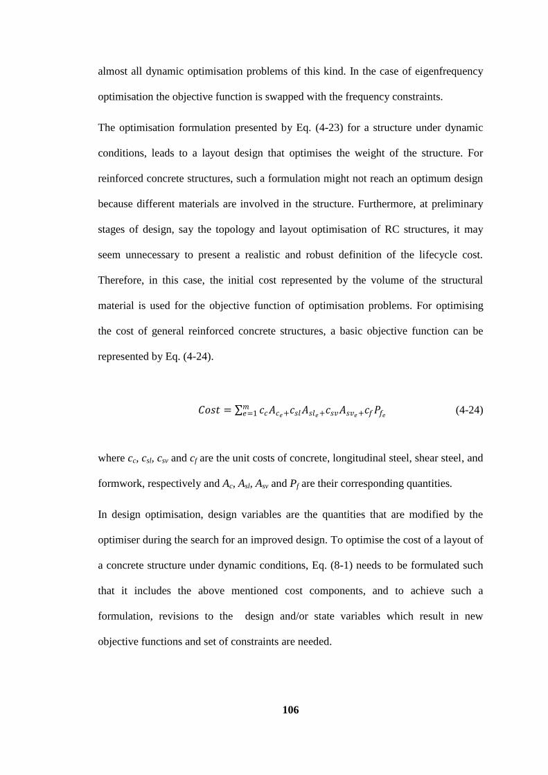
106
almost all dynamic optimisation problems of this kind. In the case of eigenfrequency
optimisation the objective function is swapped with the frequency constraints.
The optimisation formulation presented by Eq. (4-23) for a structure under dynamic
conditions, leads to a layout design that optimises the weight of the structure. For
reinforced concrete structures, such a formulation might not reach an optimum design
because different materials are involved in the structure. Furthermore, at preliminary
stages of design, say the topology and layout optimisation of RC structures, it may
seem unnecessary to present a realistic and robust definition of the lifecycle cost.
Therefore, in this case, the initial cost represented by the volume of the structural
material is used for the objective function of optimisation problems. For optimising
the cost of general reinforced concrete structures, a basic objective function can be
represented by Eq. (4-24).
𝐶𝑜𝑠𝑡 = 𝑐𝑐𝐴𝑐𝑒+𝑐𝑠𝑙𝐴𝑠𝑙𝑒+𝑐𝑠𝑣𝐴𝑠𝑣𝑒+𝑐𝑓𝑃𝑓𝑒
𝑚𝑒=1 (4-24)
where cc, csl, csv and cf are the unit costs of concrete, longitudinal steel, shear steel, and
formwork, respectively and Ac, Asl, Asv and Pf are their corresponding quantities.
In design optimisation, design variables are the quantities that are modified by the
optimiser during the search for an improved design. To optimise the cost of a layout of
a concrete structure under dynamic conditions, Eq. (8-1) needs to be formulated such
that it includes the above mentioned cost components, and to achieve such a
formulation, revisions to the design and/or state variables which result in new
objective functions and set of constraints are needed.
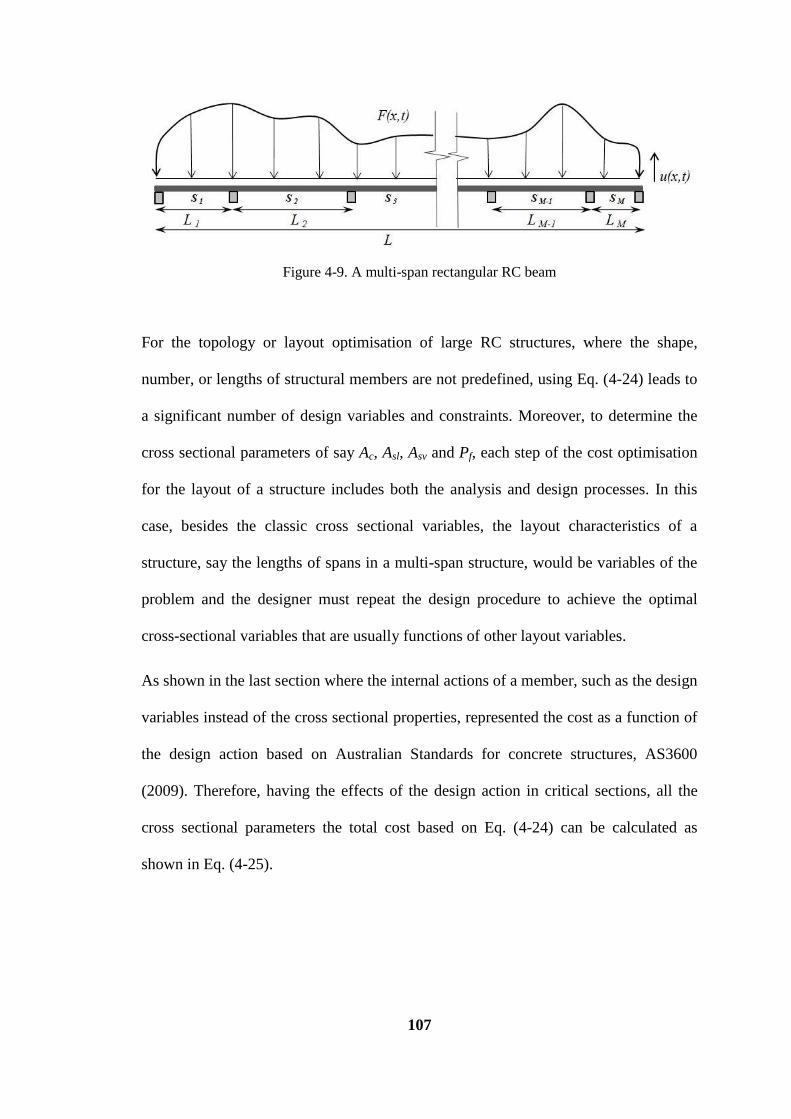
107
Figure 4-9. A multi-span rectangular RC beam
For the topology or layout optimisation of large RC structures, where the shape,
number, or lengths of structural members are not predefined, using Eq. (4-24) leads to
a significant number of design variables and constraints. Moreover, to determine the
cross sectional parameters of say Ac, Asl, Asv and Pf, each step of the cost optimisation
for the layout of a structure includes both the analysis and design processes. In this
case, besides the classic cross sectional variables, the layout characteristics of a
structure, say the lengths of spans in a multi-span structure, would be variables of the
problem and the designer must repeat the design procedure to achieve the optimal
cross-sectional variables that are usually functions of other layout variables.
As shown in the last section where the internal actions of a member, such as the design
variables instead of the cross sectional properties, represented the cost as a function of
the design action based on Australian Standards for concrete structures, AS3600
(2009). Therefore, having the effects of the design action in critical sections, all the
cross sectional parameters the total cost based on Eq. (4-24) can be calculated as
shown in Eq. (4-25).
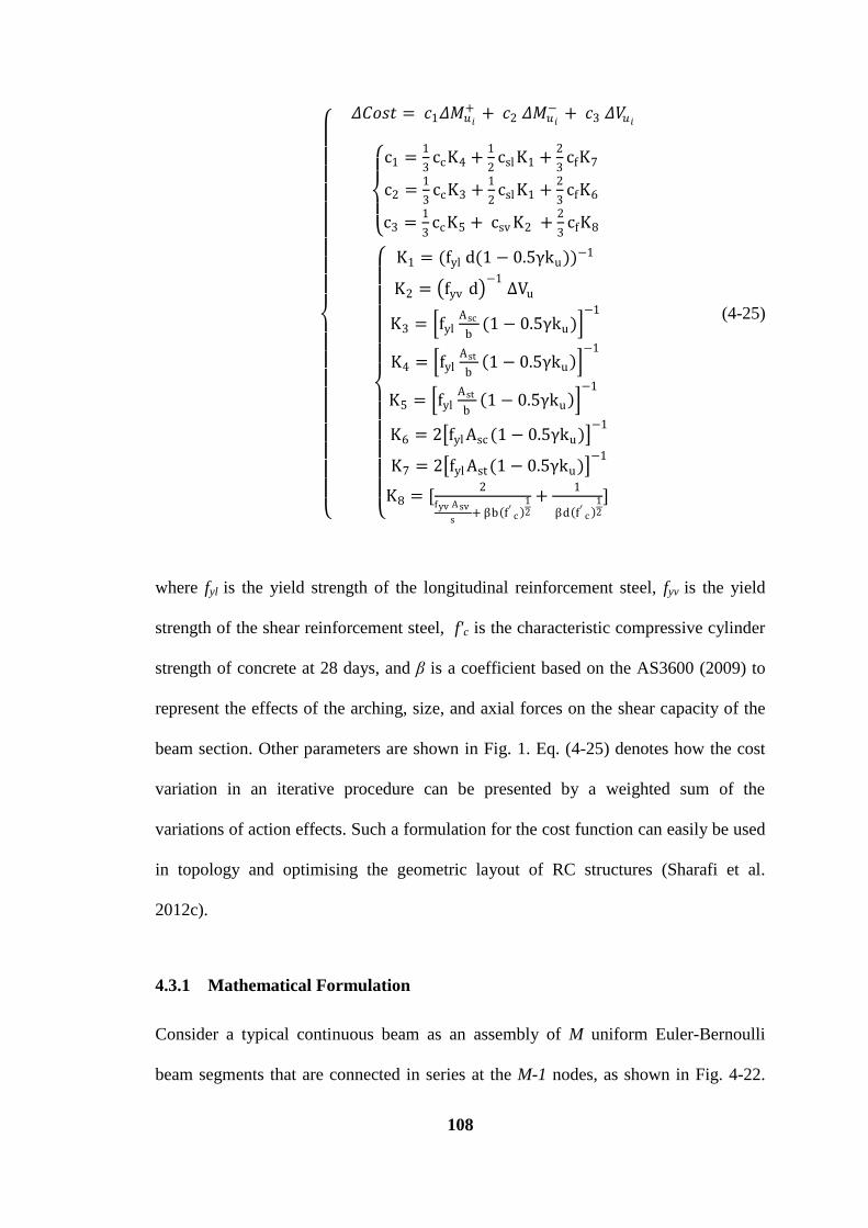
108
𝛥𝐶𝑜𝑠𝑡 = 𝑐1𝛥𝑀𝑢𝑖
+ + 𝑐2 𝛥𝑀𝑢𝑖
− + 𝑐3 𝛥𝑉𝑢𝑖
c1 =
1
3ccK4 +
1
2csl K1 +
2
3cfK7
c2 =1
3ccK3 +
1
2csl K1 +
2
3cfK6
c3 =1
3ccK5 + csv K2 +
2
3cfK8
K1 = (fyl d(1 − 0.5γku))−1
K2 = fyv d −1
∆Vu
K3 = fylAsc
b(1 − 0.5γku )
−1
K4 = fylAst
b 1 − 0.5γku
−1
K5 = fylAst
b 1 − 0.5γku
−1
K6 = 2 fyl Asc (1 − 0.5γku) −1
K7 = 2 fyl Ast (1 − 0.5γku) −1
K8 = [2
fyv A sv
s+ βb f′ c
12
+1
βd f′ c 12
]
(4-25)
where fyl is the yield strength of the longitudinal reinforcement steel, fyv is the yield
strength of the shear reinforcement steel, f'c is the characteristic compressive cylinder
strength of concrete at 28 days, and β is a coefficient based on the AS3600 (2009) to
represent the effects of the arching, size, and axial forces on the shear capacity of the
beam section. Other parameters are shown in Fig. 1. Eq. (4-25) denotes how the cost
variation in an iterative procedure can be presented by a weighted sum of the
variations of action effects. Such a formulation for the cost function can easily be used
in topology and optimising the geometric layout of RC structures (Sharafi et al.
2012c).
4.3.1 Mathematical Formulation
Consider a typical continuous beam as an assembly of M uniform Euler-Bernoulli
beam segments that are connected in series at the M-1 nodes, as shown in Fig. 4-22.
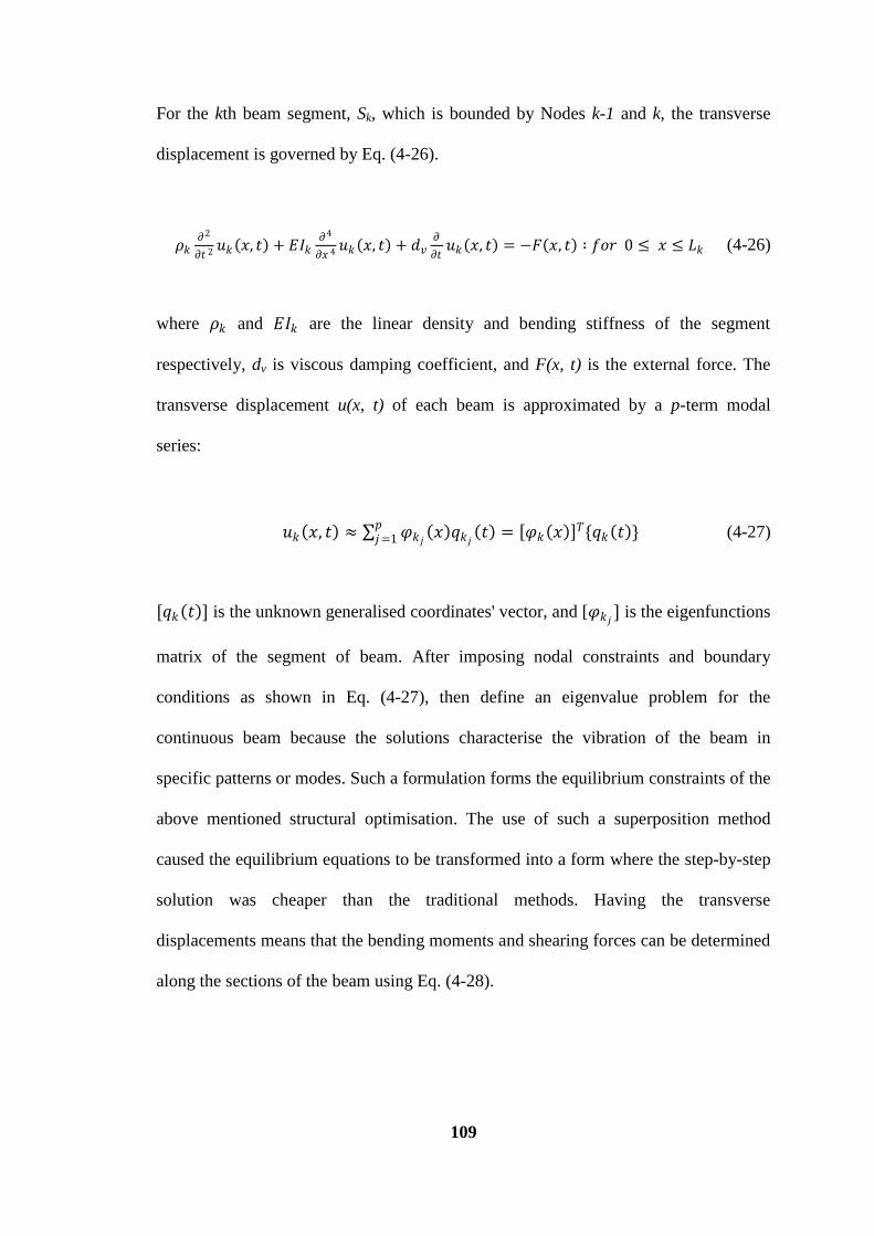
109
For the kth beam segment, Sk, which is bounded by Nodes k-1 and k, the transverse
displacement is governed by Eq. (4-26).
𝜌𝑘𝜕2
𝜕𝑡 2 𝑢𝑘 𝑥, 𝑡 + 𝐸𝐼𝑘𝜕4
𝜕𝑥 4 𝑢𝑘 𝑥, 𝑡 + 𝑑𝑣𝜕
𝜕𝑡𝑢𝑘 𝑥, 𝑡 = −𝐹 𝑥, 𝑡 ∶ 𝑓𝑜𝑟 0 ≤ 𝑥 ≤ 𝐿𝑘 (4-26)
where 𝜌𝑘 and 𝐸𝐼𝑘 are the linear density and bending stiffness of the segment
respectively, dv is viscous damping coefficient, and F(x, t) is the external force. The
transverse displacement u(x, t) of each beam is approximated by a p-term modal
series:
𝑢𝑘 𝑥, 𝑡 ≈ 𝜑𝑘𝑗 𝑥 𝑞𝑘𝑗
𝑡 = 𝜑𝑘 𝑥 𝑇{𝑞𝑘 𝑡 }𝑝𝑗=1 (4-27)
[𝑞𝑘 𝑡 ] is the unknown generalised coordinates' vector, and [𝜑𝑘𝑗] is the eigenfunctions
matrix of the segment of beam. After imposing nodal constraints and boundary
conditions as shown in Eq. (4-27), then define an eigenvalue problem for the
continuous beam because the solutions characterise the vibration of the beam in
specific patterns or modes. Such a formulation forms the equilibrium constraints of the
above mentioned structural optimisation. The use of such a superposition method
caused the equilibrium equations to be transformed into a form where the step-by-step
solution was cheaper than the traditional methods. Having the transverse
displacements means that the bending moments and shearing forces can be determined
along the sections of the beam using Eq. (4-28).
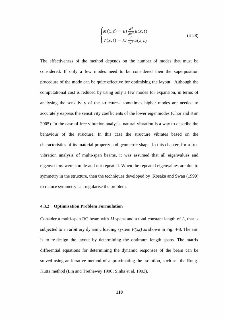
110
𝑀 𝑥, 𝑡 = 𝐸𝐼
𝜕2
𝜕𝑥 2 𝑢(𝑥, 𝑡)
𝑉 𝑥, 𝑡 = 𝐸𝐼𝜕3
𝜕𝑥 3 𝑢(𝑥, 𝑡)
(4-28)
The effectiveness of the method depends on the number of modes that must be
considered. If only a few modes need to be considered then the superposition
procedure of the mode can be quite effective for optimising the layout. Although the
computational cost is reduced by using only a few modes for expansion, in terms of
analysing the sensitivity of the structures, sometimes higher modes are needed to
accurately express the sensitivity coefficients of the lower eigenmodes (Choi and Kim
2005). In the case of free vibration analysis, natural vibration is a way to describe the
behaviour of the structure. In this case the structure vibrates based on the
characteristics of its material property and geometric shape. In this chapter, for a free
vibration analysis of multi-span beams, it was assumed that all eigenvalues and
eigenvectors were simple and not repeated. When the repeated eigenvalues are due to
symmetry in the structure, then the techniques developed by Kosaka and Swan (1999)
to reduce symmetry can regularise the problem.
4.3.2 Optimisation Problem Formulation
Consider a multi-span RC beam with M spans and a total constant length of L, that is
subjected to an arbitrary dynamic loading system F(x,t) as shown in Fig. 4-8. The aim
is to re-design the layout by determining the optimum length spans. The matrix
differential equations for determining the dynamic responses of the beam can be
solved using an iterative method of approximating the solution, such as the Rung-
Kutta method (Lin and Trethewey 1990; Sinha et al. 1993).
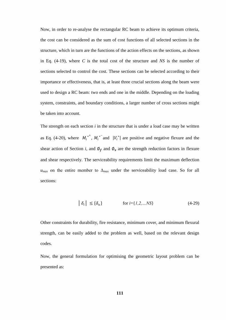
111
Now, in order to re-analyse the rectangular RC beam to achieve its optimum criteria,
the cost can be considered as the sum of cost functions of all selected sections in the
structure, which in turn are the functions of the action effects on the sections, as shown
in Eq. (4-19), where C is the total cost of the structure and NS is the number of
sections selected to control the cost. These sections can be selected according to their
importance or effectiveness, that is, at least three crucial sections along the beam were
used to design a RC beam: two ends and one in the middle. Depending on the loading
system, constraints, and boundary conditions, a larger number of cross sections might
be taken into account.
The strength on each section i in the structure that is under a load case may be written
as Eq. (4-20), where 𝑀𝑖∗+
, 𝑀𝑖∗−
and 𝑉𝑖∗ are positive and negative flexure and the
shear action of Section i, and ∅𝒇 and ∅𝒔 are the strength reduction factors in flexure
and shear respectively. The serviceability requirements limit the maximum deflection
umax on the entire member to Δmax under the serviceability load case. So for all
sections:
│𝛿𝑖│ ≤ 𝛿𝑢 for i={1,2,…NS} (4-29)
Other constraints for durability, fire resistance, minimum cover, and minimum flexural
strength, can be easily added to the problem as well, based on the relevant design
codes.
Now, the general formulation for optimising the geometric layout problem can be
presented as:
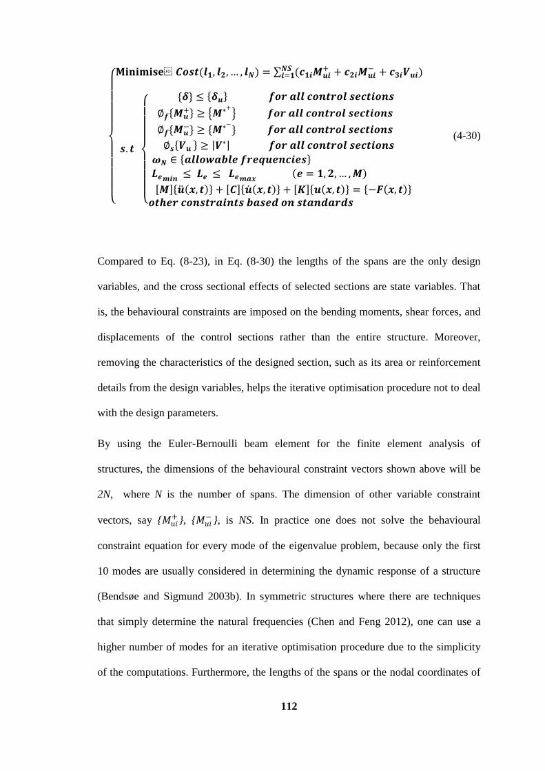
112
𝐌𝐢𝐧𝐢𝐦𝐢𝐬𝐞 𝑪𝒐𝒔𝒕(𝒍𝟏, 𝒍𝟐, … , 𝒍𝑵) = (𝒄𝟏𝒊𝑴𝒖𝒊+𝑵𝑺
𝒊=𝟏 + 𝒄𝟐𝒊𝑴𝒖𝒊− + 𝒄𝟑𝒊𝑽𝒖𝒊)
𝒔. 𝒕
{𝜹} ≤ 𝜹𝒖 𝒇𝒐𝒓 𝒂𝒍𝒍 𝒄𝒐𝒏𝒕𝒓𝒐𝒍 𝒔𝒆𝒄𝒕𝒊𝒐𝒏𝒔
∅𝒇 𝑴𝒖+ ≥ 𝑴∗+
𝒇𝒐𝒓 𝒂𝒍𝒍 𝒄𝒐𝒏𝒕𝒓𝒐𝒍 𝒔𝒆𝒄𝒕𝒊𝒐𝒏𝒔
∅𝒇{𝑴𝒖−} ≥ {𝑴∗−
} 𝒇𝒐𝒓 𝒂𝒍𝒍 𝒄𝒐𝒏𝒕𝒓𝒐𝒍 𝒔𝒆𝒄𝒕𝒊𝒐𝒏𝒔
∅𝒔 𝑽𝒖 ≥ 𝑽∗ 𝒇𝒐𝒓 𝒂𝒍𝒍 𝒄𝒐𝒏𝒕𝒓𝒐𝒍 𝒔𝒆𝒄𝒕𝒊𝒐𝒏𝒔
𝝎𝑵 ∈ 𝒂𝒍𝒍𝒐𝒘𝒂𝒃𝒍𝒆 𝒇𝒓𝒆𝒒𝒖𝒆𝒏𝒄𝒊𝒆𝒔
𝑳𝒆𝒎𝒊𝒏 ≤ 𝑳𝒆 ≤ 𝑳𝒆𝒎𝒂𝒙
𝒆 = 𝟏, 𝟐, … , 𝑴
𝑴 𝒖 𝒙, 𝒕 + 𝑪 𝒖 𝒙, 𝒕 + 𝑲 𝒖 𝒙, 𝒕 = −𝑭 𝒙, 𝒕 𝒐𝒕𝒉𝒆𝒓 𝒄𝒐𝒏𝒔𝒕𝒓𝒂𝒊𝒏𝒕𝒔 𝒃𝒂𝒔𝒆𝒅 𝒐𝒏 𝒔𝒕𝒂𝒏𝒅𝒂𝒓𝒅𝒔
(4-30)
Compared to Eq. (8-23), in Eq. (8-30) the lengths of the spans are the only design
variables, and the cross sectional effects of selected sections are state variables. That
is, the behavioural constraints are imposed on the bending moments, shear forces, and
displacements of the control sections rather than the entire structure. Moreover,
removing the characteristics of the designed section, such as its area or reinforcement
details from the design variables, helps the iterative optimisation procedure not to deal
with the design parameters.
By using the Euler-Bernoulli beam element for the finite element analysis of
structures, the dimensions of the behavioural constraint vectors shown above will be
2N, where N is the number of spans. The dimension of other variable constraint
vectors, say {𝑀𝑢𝑖+ }, {𝑀𝑢𝑖
− }, is NS. In practice one does not solve the behavioural
constraint equation for every mode of the eigenvalue problem, because only the first
10 modes are usually considered in determining the dynamic response of a structure
(Bendsøe and Sigmund 2003b). In symmetric structures where there are techniques
that simply determine the natural frequencies (Chen and Feng 2012), one can use a
higher number of modes for an iterative optimisation procedure due to the simplicity
of the computations. Furthermore, the lengths of the spans or the nodal coordinates of
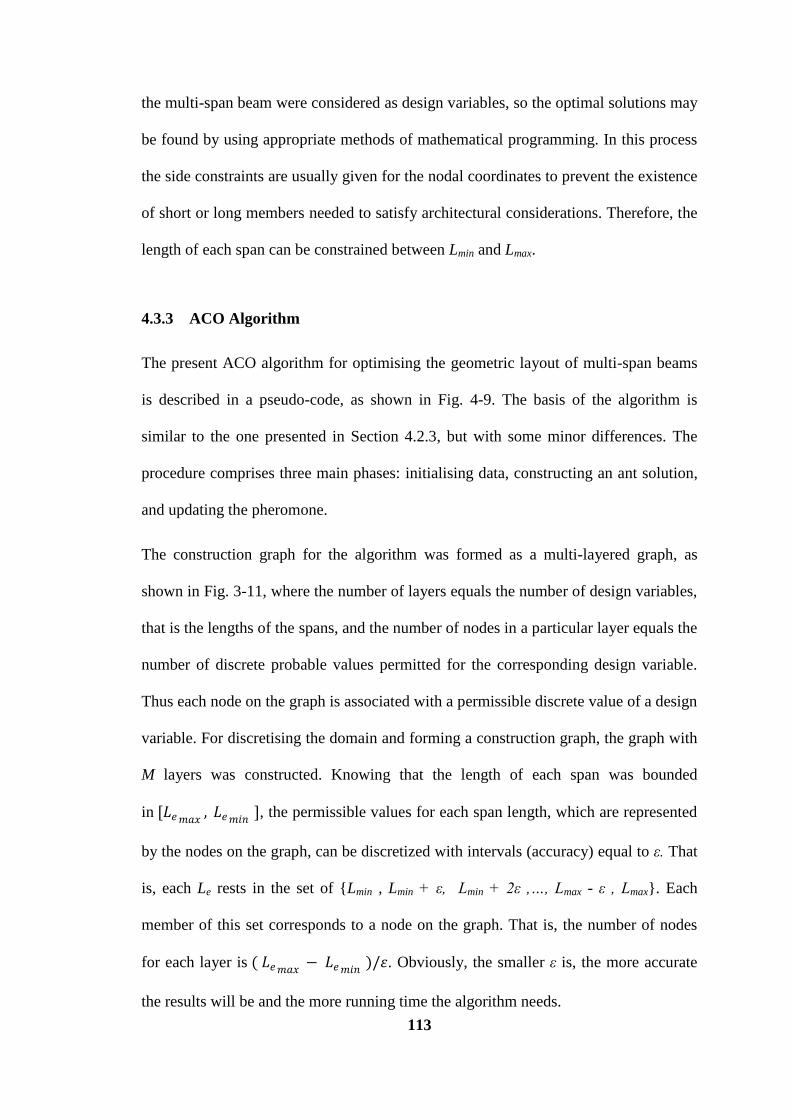
113
the multi-span beam were considered as design variables, so the optimal solutions may
be found by using appropriate methods of mathematical programming. In this process
the side constraints are usually given for the nodal coordinates to prevent the existence
of short or long members needed to satisfy architectural considerations. Therefore, the
length of each span can be constrained between Lmin and Lmax.
4.3.3 ACO Algorithm
The present ACO algorithm for optimising the geometric layout of multi-span beams
is described in a pseudo-code, as shown in Fig. 4-9. The basis of the algorithm is
similar to the one presented in Section 4.2.3, but with some minor differences. The
procedure comprises three main phases: initialising data, constructing an ant solution,
and updating the pheromone.
The construction graph for the algorithm was formed as a multi-layered graph, as
shown in Fig. 3-11, where the number of layers equals the number of design variables,
that is the lengths of the spans, and the number of nodes in a particular layer equals the
number of discrete probable values permitted for the corresponding design variable.
Thus each node on the graph is associated with a permissible discrete value of a design
variable. For discretising the domain and forming a construction graph, the graph with
M layers was constructed. Knowing that the length of each span was bounded
in [𝐿𝑒𝑚𝑎𝑥, 𝐿𝑒𝑚𝑖𝑛
], the permissible values for each span length, which are represented
by the nodes on the graph, can be discretized with intervals (accuracy) equal to ε. That
is, each Le rests in the set of {Lmin , Lmin + ε, Lmin + 2ε ,…, Lmax - ε , Lmax}. Each
member of this set corresponds to a node on the graph. That is, the number of nodes
for each layer is ( 𝐿𝑒𝑚𝑎𝑥− 𝐿𝑒𝑚𝑖𝑛
)/휀. Obviously, the smaller ε is, the more accurate
the results will be and the more running time the algorithm needs.

114
The heuristic values are specified according to the designers' preferences. As an
example in this case, if there are any preferences for certain length spans due to
architectural constraints say, higher values are assigned to the heuristic arrays that
correspondto those length spans. Such an assignment means that it will be more likely
that the desired will be chosen by ants for the corresponding spans. Then by choosing
appropriate values for α and β the degree of influence of the heuristic values compared
to the pheromone trail was determined. Moreover, in order to save time, criteria such
as the symmetry of the beam were considered when the heuristic matrix was formed.
Using such a heuristic matrix or defining the initial pheromone matrix using the above
mentioned structural rules helps the algorithm to converge sooner.
The initial magnitude of pheromone on the construction graph must be set. A good
heuristic that would initialise the pheromone trails is to set them to a value slightly
higher than the amount of pheromone that the ants are expected to deposit in one
iteration. A rough estimate of the value can be obtained by setting, ∀ 𝑖, 𝑗 𝜏𝑖𝑗 = 𝜏0 =
𝑁/𝐶𝑛𝑛 where N is the number of ants, and Cnn
is the cost of a tour generated by the
nearest neighbouring heuristic (Kaveh and Sharafi 2008a; b; 2009). As boundary
conditions and constraints, plus any loads can affect the length of spans, the entries of
the heuristic matrix and initial pheromone matrix might be organised based on such
parameters. Thus, each value (i,j) of the choice information matrix, which was
obtained by multiplying the corresponding arrays of heuristic matrix by those of
pheromone matrix, showed the tendency or desirability of the ant located on Node i of
the construction graph to choose Edge j and move towards Node i+1.
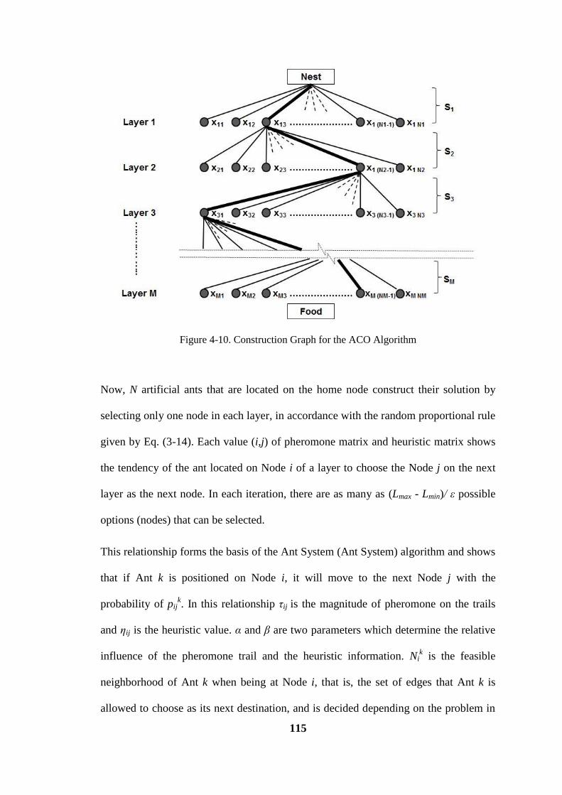
115
Figure 4-10. Construction Graph for the ACO Algorithm
Now, N artificial ants that are located on the home node construct their solution by
selecting only one node in each layer, in accordance with the random proportional rule
given by Eq. (3-14). Each value (i,j) of pheromone matrix and heuristic matrix shows
the tendency of the ant located on Node i of a layer to choose the Node j on the next
layer as the next node. In each iteration, there are as many as (Lmax - Lmin)/ ε possible
options (nodes) that can be selected.
This relationship forms the basis of the Ant System (Ant System) algorithm and shows
that if Ant k is positioned on Node i, it will move to the next Node j with the
probability of pijk. In this relationship τij is the magnitude of pheromone on the trails
and ηij is the heuristic value. α and β are two parameters which determine the relative
influence of the pheromone trail and the heuristic information. Nik is the feasible
neighborhood of Ant k when being at Node i, that is, the set of edges that Ant k is
allowed to choose as its next destination, and is decided depending on the problem in

116
hand. The nodes selected along the path that were visited by an ant represent a
candidate solution.
Using the information obtained in the phase of constructing the solution, the trail that
presented the best cost up to this stage was selected as the best iteration so far. Then
pheromone trails of the construction graph were then updated by first lowering the
pheromone value on all arcs (pheromone evaporation), and then adding pheromone on
the edges the ants have crossed (pheromone depositing). Pheromone evaporation is
done by lowering the pheromone value on all edges by a constant factor ρ according to
Eq. (3-15). Then, once the path is complete, the ant deposits some pheromone on the
path based on the rule given by Eq. (3-16), where Δτijk is the pheromone added to τij by
Ant k, and defined as eq. (3.17). As such, in each iteration, all the ants ard in parallel
and start from the home node and end at the destination node by randomly selecting a
node in each layer. The optimisation process is terminated if no better solution is
found in a pre-specified number of successive iterations.
4.3.4 Numerical Examples
In order to evaluate the effects of the geometric layout on cost, and to demonstrate the
robustness of the proposed approach, a general multi-span beam under different
loading conditions was examined. The optimum geometric layout of the beam was
designed under two loading system; first a static Uniformly Distributed Load (UDL),
and second a moving point load along the beam. The results were then compared with
those obtained from an eigenvalue optimisation method which was presented by
Achtziger and Kočvara 2007. Since the eigenvalue optimisation method did not
necessarily optimise the costs, this method is only considered as a benchmark and a
starting point for the algorithm. That is, optimise the topology first using the
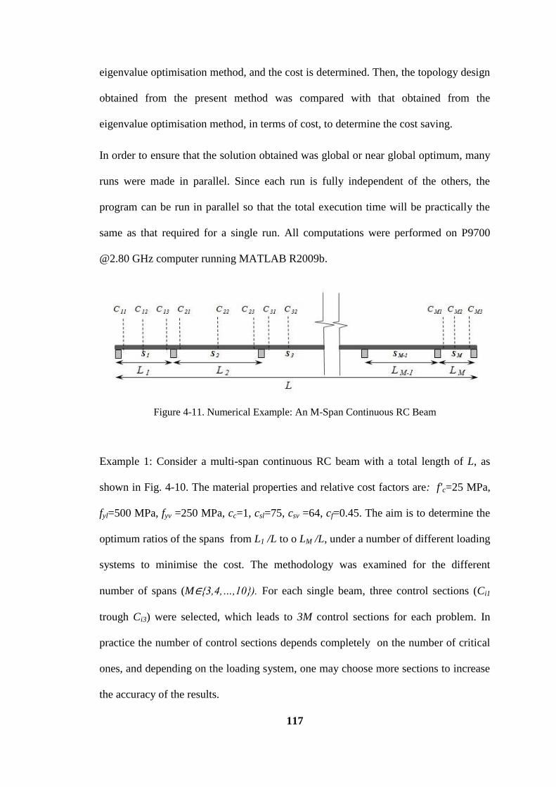
117
eigenvalue optimisation method, and the cost is determined. Then, the topology design
obtained from the present method was compared with that obtained from the
eigenvalue optimisation method, in terms of cost, to determine the cost saving.
In order to ensure that the solution obtained was global or near global optimum, many
runs were made in parallel. Since each run is fully independent of the others, the
program can be run in parallel so that the total execution time will be practically the
same as that required for a single run. All computations were performed on P9700
@2.80 GHz computer running MATLAB R2009b.
Figure 4-11. Numerical Example: An M-Span Continuous RC Beam
Example 1: Consider a multi-span continuous RC beam with a total length of L, as
shown in Fig. 4-10. The material properties and relative cost factors are: f'c=25 MPa,
fyl=500 MPa, fyv =250 MPa, cc=1, csl=75, csv =64, cf=0.45. The aim is to determine the
optimum ratios of the spans from L1 /L to o LM /L, under a number of different loading
systems to minimise the cost. The methodology was examined for the different
number of spans (M∈{3,4,…,10}). For each single beam, three control sections (Ci1
trough Ci3) were selected, which leads to 3M control sections for each problem. In
practice the number of control sections depends completely on the number of critical
ones, and depending on the loading system, one may choose more sections to increase
the accuracy of the results.

118
Figure 4-12. A multi-span beam and the coresponding construction graph the algorithm
The boundary conditions and support constraints were set based on the fact that all the
supports act like perfect hinges. An average viscous damping ratio of ξ=0.03 was
considered for the whole structure (Adams and Askenazi 1999), and to approximate
the solution of the matrix differential equations, the Runge-Kutta algorithm was used.
Every initial design based on the preliminary judgment of the designer and/or using
approximate charts or formulas, and which meet the requirements of the design code,
can be used as the initial design and as the starting point for the optimisation process.
For this problem the case of designing for a maximum fundamental eigenvalue for free
vibration was considered as an initial design and as a benchmark with which to
compare the results. For this purpose the layout of the beam was optimised in order to
maximise the fundamental eigenfrequency for all cases and where the results were
considered to be the starting point for the optimisation problem. The results showed
that for such a continuous beam, the case of maximum fundamental eigenfrequency
lead to identical spans for all cases. That is, the continuous beams where all the spans
are identical have the maximum fundamental eigenfrequency among the other possible
layout designs. Having the initial design and using Eq. (4-25), the values of K1 to K8,
119
and then the values of c1, c2 and c3 for Sections A to O were obtained, and now that the
necessary coefficients are available, the cost function can be defined.
Two different loading systems were considered and the optimum layout designs were
obtained for each one independently. The first one was a uniformly distributed static
load and the second case was a point wise load of 100 kN moving along the beam at a
speed of 2 m/sec from x=0 to x=L. As mentioned above, the designs for all
caseswhere all the spans were equal to L/M, the corresponding costs were considered
as the initial design and the starting point for the algorithm.
For the initial design of the layout with the maximum eigenvalue, the ratios of the
spans which resulted in the maximum fundamental eigenvalue was taken. For case one
and the static loading the equilibrium constraint in Eq. (4-25) turned to the static
condition [K]{u(x)}={Fst}. In this example the behavioural constraint on natural
frequency was not required for either static or dynamic loading. In the second case the
dynamic load was formulated as:
F(x,t)= -δ(x-vt)P (4-31)
Where δ is a Dirac delta function, v is the constant speed of the load motion, which in
this case is 2 m/s, and P is the weight of the moving object which is 100 kN.
In the construction graph phase the span lengths, as the problem domain, were
discretised and a number of possible lengths were considered for each span. For this
purpose the maximum and minimum possible span lengths and the problem accuracy
(ε) were defined, and a construction graph produced (see Fig. 4-9), after which ants
were located on the starting and ending nodes to make their trails in parallel. The
reason why two groups of ants were used was to give all the spans the same
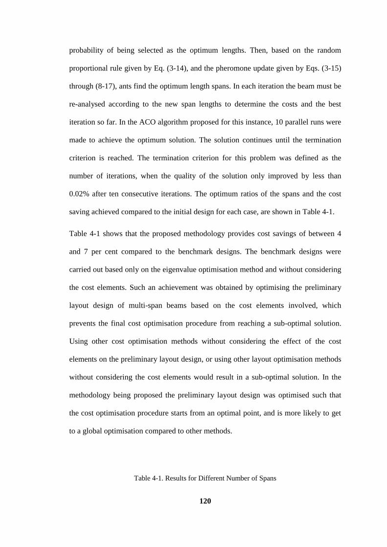
120
probability of being selected as the optimum lengths. Then, based on the random
proportional rule given by Eq. (3-14), and the pheromone update given by Eqs. (3-15)
through (8-17), ants find the optimum length spans. In each iteration the beam must be
re-analysed according to the new span lengths to determine the costs and the best
iteration so far. In the ACO algorithm proposed for this instance, 10 parallel runs were
made to achieve the optimum solution. The solution continues until the termination
criterion is reached. The termination criterion for this problem was defined as the
number of iterations, when the quality of the solution only improved by less than
0.02% after ten consecutive iterations. The optimum ratios of the spans and the cost
saving achieved compared to the initial design for each case, are shown in Table 4-1.
Table 4-1 shows that the proposed methodology provides cost savings of between 4
and 7 per cent compared to the benchmark designs. The benchmark designs were
carried out based only on the eigenvalue optimisation method and without considering
the cost elements. Such an achievement was obtained by optimising the preliminary
layout design of multi-span beams based on the cost elements involved, which
prevents the final cost optimisation procedure from reaching a sub-optimal solution.
Using other cost optimisation methods without considering the effect of the cost
elements on the preliminary layout design, or using other layout optimisation methods
without considering the cost elements would result in a sub-optimal solution. In the
methodology being proposed the preliminary layout design was optimised such that
the cost optimisation procedure starts from an optimal point, and is more likely to get
to a global optimisation compared to other methods.
Table 4-1. Results for Different Number of Spans
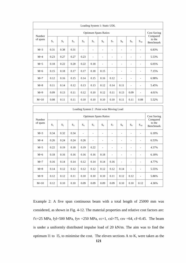
121
Loading System 1: Static UDL
Number
of spans
Optimum Spans Ratios Cost Saving
Compared
to the
Benchmark S1 S2 S3 S4 S5 S6 S7 S8 S9 S10
M=3 0.31 0.38 0.31 - - - - - - - 6.83%
M=4 0.23 0.27 0.27 0.23 - - - - - - 5.53%
M=5 0.18 0.22 0.20 0.22 0.18 - - - - - 6.05%
M=6 0.15 0.18 0.17 0.17 0.18 0.15 - - - - 7.15%
M=7 0.12 0.16 0.15 0.14 0.15 0.16 0.12 - - - 6.98%
M=8 0.11 0.14 0.12 0.13 0.13 0.12 0.14 0.11 - - 5.45%
M=9 0.09 0.13 0.11 0.12 0.10 0.12 0.11 0.13 0.09 - 4.01%
M=10 0.08 0.11 0.11 0.10 0.10 0.10 0.10 0.11 0.11 0.08 5.52%
Loading System 2 : Point wise Moving Load
Number
of spans
Optimum Spans Ratios Cost Saving
Compared
to the
Benchmark S1 S2 S3 S4 S5 S6 S7 S8 S9 S10
M=3 0.34 0.32 0.34 - - - - - - - 6.18%
M=4 0.26 0.24 0.24 0.26 - - - - - - 6.53%
M=5 0.22 0.19 0.18 0.19 0.22 - - - - - 4.57%
M=6 0.18 0.16 0.16 0.16 0.16 0.18 - - - - 6.18%
M=7 0.16 0.14 0.14 0.12 0.14 0.14 0.16 - - - 4.77%
M=8 0.14 0.12 0.12 0.12 0.12 0.12 0.12 0.14 - - 5.55%
M=9 0.12 0.12 0.11 0.10 0.10 0.10 0.11 0.12 0.12 - 5.86%
M=10 0.12 0.10 0.10 0.09 0.09 0.09 0.09 0.10 0.10 0.12 4.36%
Example 2: A five span continuous beam with a total length of 25000 mm was
considered, as shown in Fig. 4-12. The material properties and relative cost factors are:
f'c=25 MPa, fyl=500 MPa, fyv =250 MPa, cc=1, csl=75, csv =64, cf=0.45. The beam
is under a uniformly distributed impulse load of 20 kN/m. The aim was to find the
optimum l1 to l5, to minimise the cost. The eleven sections A to K, were taken as the

122
control sections. The number of sections selected depends completely on the number
of critical or control ones, and more sections may be chosen to achieve more accurate
results.
Figure 4-13. Example: a five span beam and selected sections to control the cost
The preliminary design of the beam comprised five equal spans, which resulted in a
total cost of 6967 units. It should be added that every initial design based on the
preliminary judgment of the designer and/or using approximate charts or formulae
which meet the design code requirements, can be used as the initial design and as the
starting point of the optimisation process. The values of K1 to K8, and then the values
of c1, c2, and c3 for sections A to K were obtained. Having the necessary coefficients,
the cost function can be defined based on Eq. (4-30).
The Ant algorithm attempts to find the optimum length spans using Eq. (4-30) as its
objective function and by observing other relevant constraints. Using the proposed Ant
algorithm, after 125 iterations and at a CPU time of 31.59 seconds, the optimum
lengths of l1 = 4800 mm, l2 =4100 mm, l3 =6900 mm, l4 =4200 mm and l5 =5000
mm were obtained, resulting in a total cost of 5833 units, based on Eq. (4-23), which
equals a 16.2% cost saving. The interesting point here is if an equivalent static load
123
was used in lieu of the impulse load, the optimum span lengths of 4000, 5900, 5200,
5900, 4000 at the cost of 5648 would be obtained. This shows that the dynamic
analysis resulted in a further 3.2 % cost. Fig. 4-13 shows a typical convergence history
for the ACO algorithm for this example.
Figure 4-14. Typical convergence history for the presented ACO algorithm
4.4 Summary
The main objective of this chapter was to propose an appropriate model to optimise
the cost of RC beams layout design under static and dynamic loading. This model
considered the effects of the layout design on total cost and suggested a method for
optimising the layout design of multi-span beams. Using action effects instead of the
cross sectional properties of structures, the proposed model simplifies the process of
optimising the cost and layout of multi-span beams, and is therefore applicable to
124
various topology optimisation problems of RC beams when the cost elements are
considered. The algorithm proposed for solving the layout optimisation problem is an
Ant System based algorithm which can easily be used to optimise span lengths, and
can also work with different cost functions to optimise the layout of multi-span beams.
The examples used showed that using the new cost optimisation function with the
proposed algorithm provided acceptable results, and can be easily be used to optimally
design the preliminary layout of RC continuous beams.
125
5 Optimum Column Layout Design of Plane Frames under
Wind Loading
5.1 Introduction
This chapter presents a heuristic approach for optimising the layout design of two-
dimensional reinforced concrete frames in order to optimise their total cost and control
them under wind loadings. The aim was to find the optimum column layout for plane
frames under wind loadings while considering the cost elements involved. A heuristic
methodology was developed to achieve a new design space and an objective function
for optimising the cost and layout. The proposed method can make use of the action
effects of the structure as alternative design variables in place of the commonly used
cross sectional ones. Such a feature gives this method the ability to be used in large
and realistic structural optimisation problems and also helps the optimisation
algorithms take less time in an iterative optimisation process. An Ant System based
algorithm was then proposed to solve the optimisation problem presented, which also
includes examples to illustrate the robustness of the methodology.
As noted in previous chapters, one of the most important phases in the optimal design
process is the selection of the cost function, which is generally a function of the design
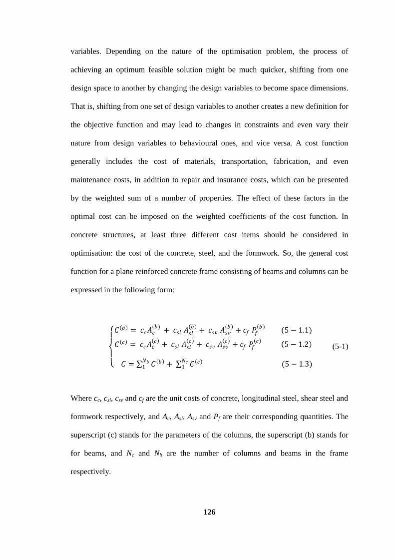
126
variables. Depending on the nature of the optimisation problem, the process of
achieving an optimum feasible solution might be much quicker, shifting from one
design space to another by changing the design variables to become space dimensions.
That is, shifting from one set of design variables to another creates a new definition for
the objective function and may lead to changes in constraints and even vary their
nature from design variables to behavioural ones, and vice versa. A cost function
generally includes the cost of materials, transportation, fabrication, and even
maintenance costs, in addition to repair and insurance costs, which can be presented
by the weighted sum of a number of properties. The effect of these factors in the
optimal cost can be imposed on the weighted coefficients of the cost function. In
concrete structures, at least three different cost items should be considered in
optimisation: the cost of the concrete, steel, and the formwork. So, the general cost
function for a plane reinforced concrete frame consisting of beams and columns can be
expressed in the following form:
𝐶 𝑏 = 𝑐𝑐𝐴𝑐
(𝑏) + 𝑐𝑠𝑙 𝐴𝑠𝑙
(𝑏)+ 𝑐𝑠𝑣 𝐴𝑠𝑣
𝑏 + 𝑐𝑓 𝑃𝑓
𝑏 (5 − 1.1)
𝐶 𝑐 = 𝑐𝑐𝐴𝑐 𝑐
+ 𝑐𝑠𝑙 𝐴𝑠𝑙 𝑐
+ 𝑐𝑠𝑣 𝐴𝑠𝑣 𝑐
+ 𝑐𝑓 𝑃𝑓 𝑐
5 − 1.2
𝐶 = 𝐶 𝑏 𝑁𝑏1 + 𝐶 𝑐 𝑁𝑐
1 (5 − 1.3)
(5-1)
Where cc, csl, csv and cf are the unit costs of concrete, longitudinal steel, shear steel and
formwork respectively, and Ac, Asl, Asv and Pf are their corresponding quantities. The
superscript (c) stands for the parameters of the columns, the superscript (b) stands for
for beams, and Nc and Nb are the number of columns and beams in the frame
respectively.
127
In Chapter 2 it was stated that in most published studies the cost optimisation
functions only deal with cross sectional variables which mainly suits structures with a
small number of members and a predefined geometric layout. In fact, in the layout
design of structures, the cross sectional variables are functions of design action effects
which are not determinate and vary as the shape changes. Therefore, in an iterative
procedure to solve an optimisation problem, each step includes dealing with both the
structural analysis and structural design variables. In cases such as these, unless
alternative design variables are selected for the cost function, the optimisation
procedure might be too unwieldy.
As discussed in Section 4, while parameters like the cross sectional variables are
mainly obtained from implicit functions of structural analysis outputs based on the
relationships and constraints suggested in the design standards, design standards do
not provide the exact values for these cross-sectional parameters and they are not
obtained from an explicit mathematical procedure. That is, in a layout optimisation
problem that considers the cost elements apart from the classic cross sectional
variables, the layout of a structure and consequently the outputs of structural analysis
would be the variables of the problem. If the reciprocal relationships between the cross
sectional design factors and the design action effects are determined, the cost function
can be presented by a function of the design action effects. In the design process the
design action effects for the critical sections of members are determined and then the
cross sectional variables for each section are calculated. Cross sectional parameters
along the structural members are obtained from their value in critical sections and are
based on the relationships in the design standards. In fact by having the design action
effects in critical sections, all the cross sectional parameters and the total cost based on
Eq. (5-1) can be calculated. To put it simply, using the structural analysis outputs of
128
say the internal actions of a member as design variables, has some advantages over
using structural design outcomes such as the cross sectional characteristics of a beam.
Firstly, the design action effects of each section can easily be obtained from a
structural analysis, and re-analysing a structure in an iterative mathematical procedure
is considerably less time consuming and more precise than re-designing the structure.
Moreover, by using action effects the cost function will be considered in a section
rather than a member. this enables the designer to select a number of sections for each
member and control the cost in the whole structure, so there is no need to conduct an
optimisation process over the entire member.
Therefore the aim of this chapter was to explore the relationship between the variation
of action effects of RC members with variations of the cross sectional parameters in
plane frames, and determine how these two types of variables affect each other. Then,
based on these relationships, a new cost function was obtained which is a function of
the action effects rather than the cross sectional parameters.
In order to formulate the structural optimisation problem this study made use of the
relationships in the Australian standards for concrete structures (AS3600-2009) and
Structural design actions for wind (AS/NZS1170.2-2011), which is based on the
limited state design method for concrete structures. Frames consist of two groups of
structural elements: beams and columns; both of which have key roles in the total cost
of a frame.
5.2 Mathematical formulation
To design a beam means takinig three action effects into consideration: the positive
bending moment, the negative bending moment, and the shear forces. Let us consider

129
an arbitrary section of a rectangular reinforced concrete beam, as shown in Fig. 4.1.
The dimensions of the section are b and h(b)
, the areas of tension and compression
reinforcement are 𝐴𝑠𝑡(𝑏)
, 𝐴𝑠𝑐(𝑏)
and the area of shear reinforcement in a unit length of
beam is 𝐴𝑠𝑣(𝑏)
/𝑠.
Now, consider Eq. (4-3) as a potential alternative cost function to Eq. (5-1.1) in an
arbitrary RC beam section.
The capacity or the ultimate strength of the section in negative and positive flexure
and shear for section i are 𝑀𝑢𝑖
− (𝑏) , 𝑀𝑢𝑖
+ (𝑏) and 𝑉𝑢𝑖
(𝑏) respectively, which can be
obtained from Eq. (5-2) through Eq. (5-4) in a balanced section in which both tension
and compression steel yield.
𝑀𝑢+ (𝑏)
≅ 𝐴𝑠𝑐 𝑏
𝑓𝑦𝑙 𝑑(𝑏) − 𝑑𝑐
(𝑏) + (𝐴𝑠𝑡 𝑏
− 𝐴𝑠𝑐 𝑏
)𝑓𝑦𝑙 𝑑(𝑏) − 𝑎/2 (5-2)
𝑀𝑢
− (𝑏) ≅ 𝐴𝑠𝑐
𝑏 𝑓𝑦𝑙 (𝑑
(𝑏) − 𝑑𝑐(𝑏))
𝑑𝑐(𝑏) = 0.5𝛾𝑘𝑢 𝑑
𝑏 (5-3)
𝑉𝑢 (𝑏)
≅𝑓𝑦𝑣 𝑑𝐴𝑠𝑣
𝑏
𝑠+ 𝛽𝑏𝑑(𝑏)(𝑓𝑐
′)0.5 (5-4)
where fyl is the yield strength of the longitudinal reinforcement, fyv is the yield strength
of the shear reinforcement, f'c is the characteristic compressive cylinder strength of
concrete at 28 days, 𝑑𝑐(𝑏)
is the distance from the extreme compression fibre of the
concrete to the compressive force. The coefficients 𝛾 and 𝑘𝑢 were calculated based on
the characteristic strength of the concrete and reinforcing steel, β is a coefficient based
130
on the standard, and s is the centre-to-centre spacing of shear reinforcement. Other
parameters are shown in Fig. 4-1.
Design standards impose some upper and lower bounds for the amount of longitudinal
and shear reinforcement, and consequently the value of the bearing capacities that
must be considered. In this chapter the doubly reinforced condition, as an inclusive
case, was considered. In case of singular reinforcement the current methodology
could easily be used by considering 𝐴𝑠𝑐(𝑏)
=0.
In order to shift from Eq. (5-2.1) to Eq. (5-2.3) and come up with the set of {c1, c2, c3},
the first step was to determine how the cross sectional variations of 𝐴𝑐 𝑏
, 𝐴𝑠𝑙 𝑏
, 𝐴𝑠𝑣 𝑏
and
𝑃𝑓 𝑏
would affect the section bearing capacities 𝑀𝑢+ (𝑏)
, 𝑀𝑢− (𝑏)
and 𝑉𝑢(𝑏)
, and vice
versa. That is, the reciprocal relationships between these two sets of variables must be
determined in order to find out how varying the amount of each cross sectional
parameter influences the section bearing capacities, and how to change the cross
sectional parameters to vary the section capacities. Given the unit costs cc, csl, csv and
cf, the cost function can be defined using Eq. (5-2.1) for each section of a beam. The
parameters 𝐴𝑐 𝑏
, 𝐴𝑠𝑙 𝑏
, 𝐴𝑠𝑣 𝑏
and 𝑃𝑓 𝑏
are obtained from the sum of the cross sectional
variables for all beams. If any of the cross sectional parameters change, the cost
function varies as follows
𝛥𝐶 𝑏 = 𝑐𝑐𝛥𝐴𝑐(𝑏)
+ 𝑐𝑠𝑙 𝛥𝐴𝑠𝑙(𝑏)
+ 𝑐𝑠𝑣 𝛥𝐴𝑠𝑣 𝑏
+ 𝑐𝑓 𝛥𝑃𝑓 𝑏
(5-5)
On the other hand, using Eq. (6-6) variations in the section capacities would change
the cost function as follows:
131
𝛥𝐶 𝑏 = 𝑐1𝛥𝑀𝑢𝑖
+ 𝑏 + 𝑐2 𝛥𝑀𝑢𝑖
− 𝑏 + 𝑐3 𝛥𝑉𝑢𝑖
𝑏 (5-6)
Eqs. (5-5) and (5-6) show the contribution of each factor to the cost changes and the
sensitivity of the cost to each term. For example, changing a unit of 𝐴𝑐 𝑏
causes a
change of cc units in cost. Therefore, if the effect of variations of 𝐴𝑐 𝑏
, 𝐴𝑠𝑙 𝑏
, 𝐴𝑠𝑣 𝑏
and
𝑃𝑓 𝑏
on the variations of 𝑀𝑢+ (𝑏)
, 𝑀𝑢− (𝑏)
and 𝑉𝑢(𝑏)
are determined, the contribution of
each section capacity to cost changes, that is the set of {c1, c2, c3}, can be determined.
To simplify the calculations, two assumptions were made. First, since we intend the
section to remain in a balanced condition, any changes in the amount of compression
steel reinforcement were considered to equal those of tension steel reinforcement.
Δ𝐴𝑠𝑡 𝑏
= Δ𝐴𝑠𝑐 𝑏
= Δ𝐴𝑠𝑙 𝑏
(5-7)
The second assumption was that the depth of the compressive region of concrete, the
variable a, was not significantly affected by variations of the section width b. The
width of a beam section is generally constrained by a number of factors including
architectural constraints, standards limitations, and the limitations of columns and
joints. All these constraints caused the width of the section to have a minor variation
during the optimisation process. This does not mean that the variation of width was
ignored, but in practice such a variation is so limited that it has a negligible effect on
the depth of the compressive region. Moreover, since the cover to steel reinforcement
was considered to be constant, variations in the section height equal the variations of
d(b)
.
132
Any changes in the longitudinal steel 𝐴𝑠𝑙(𝑏)
results in changes in the capacities of a
beam section as follows:
𝛥𝑀𝑢− 𝑏
𝛥𝐴𝑠𝑙 𝑏 ≅ 𝑓𝑦𝑙 𝑑
(𝑏) − 𝑑𝑐(𝑏) → 𝛥𝐴𝑠𝑙
𝑏 = (𝑓𝑦𝑙 𝑑
𝑏 (1 − 0.5𝛾𝑘𝑢 ))−1 𝛥𝑀𝑢− 𝑏
= 𝐾1 𝛥𝑀𝑢− 𝑏
𝛥𝑀𝑢+ 𝑏
𝛥𝐴𝑠𝑙 𝑏 ≅ 𝑓𝑦𝑙 𝑑
(𝑏) − 𝑑𝑐(𝑏) → 𝛥𝐴𝑠𝑙
𝑏 = (𝑓𝑦𝑙 𝑑
𝑏 (1 − 0.5𝛾𝑘𝑢 ))−1 𝛥𝑀𝑢+ 𝑏
= 𝐾1 𝛥𝑀𝑢+ 𝑏
∆𝑉𝑢(𝑏)
𝛥𝐴𝑠𝑙 𝑏 ≅ 0 → ∆𝑉𝑢
(𝑏) 𝑎𝑛𝑑 𝛥𝐴𝑠𝑙 𝑎𝑟𝑒 𝑖𝑛𝑑𝑒𝑝𝑒𝑛𝑑𝑒𝑛𝑡 𝑜𝑓 𝑒𝑎𝑐 𝑜𝑡𝑒𝑟
(5-8)
If 𝐴𝑠𝑣(𝑏)
/𝑠 changes the variation of the beams bearing capacities are
𝛥𝑀𝑢
− 𝑏 𝑎𝑛𝑑
𝛥𝐴𝑠𝑣 𝑏
𝑠 𝑎𝑟𝑒 𝑖𝑛𝑑𝑒𝑝𝑒𝑛𝑑𝑒𝑛𝑡 𝑜𝑓 𝑒𝑎𝑐 𝑜𝑡𝑒𝑟
𝛥𝑀𝑢+ 𝑏
𝑎𝑛𝑑 𝛥𝐴𝑠𝑣
𝑏
𝑠 𝑎𝑟𝑒 𝑖𝑛𝑑𝑒𝑝𝑒𝑛𝑑𝑒𝑛𝑡 𝑜𝑓 𝑒𝑎𝑐 𝑜𝑡𝑒𝑟
∆𝑉𝑢(𝑏)
𝛥𝐴𝑠𝑣 𝑏
𝑠
≅ 𝑓𝑦𝑣𝑑 → 𝛥𝐴𝑠𝑣
𝑏
𝑠≅ (𝑓𝑦𝑣 𝑑)−1 ∆𝑉𝑢
(𝑏)= 𝐾2 ∆𝑉𝑢
(𝑏)
(5-9)
If the effective area of the beam section ∆𝐴𝑐(𝑏)
, i.e. bd varies:
∆𝑨𝒄(𝒃)
= Δ(bd) =b Δd + d Δb + Δb Δd = b Δd (5-10)
𝛥𝑀𝑢− 𝑏
is not a function of b, and based on the second assumption, the dependence of
𝛥𝑀𝑢+ 𝑏
on the changes of b is neglected. Moreover, the first term of 𝑉𝑢(𝑏)
is not
dependent on b as well. So, the variations of the section capacities due to variation of
cross-section area are
𝛥𝑀𝑢 𝑏
∆𝐴𝑐 𝑏 =
𝛥𝑀𝑢 𝑏
𝛥 𝑏𝑑 ≅
𝛥𝑀𝑢 𝑏
𝑏 𝛥𝑑 (5-11)

133
𝛥𝑀𝑢
− 𝑏
𝛥(𝑏𝑑(𝑏))≅
𝑓𝑦𝑙 𝐴𝑠𝑐(𝑏)
𝑏(1 − 0.5𝛾𝑘𝑢 ) → ∆𝐴𝑐
(𝑏)= 𝛥 𝑏𝑑(𝑏) ≅ 𝑓𝑦𝑙
𝐴𝑠𝑐(𝑏)
𝑏(1 − 0.5𝛾𝑘𝑢 )
−1
𝛥𝑀𝑢− 𝑏
= 𝐾3 𝛥𝑀𝑢− 𝑏
𝛥𝑀𝑢+ 𝑏
𝛥(𝑏𝑑(𝑏))≅
𝑓𝑦𝑙 𝐴𝑠𝑡(𝑏)
𝑏(1 − 0.5𝛾𝑘𝑢 ) → ∆𝐴𝑐
(𝑏)= 𝛥 𝑏𝑑(𝑏) ≅ 𝑓𝑦𝑙
𝐴𝑠𝑡(𝑏)
𝑏(1 − 0.5𝛾𝑘𝑢 )
−1
𝛥𝑀𝑢+ 𝑏
= 𝐾4 𝛥𝑀𝑢+ 𝑏
∆𝑉𝑢(𝑏)
𝛥(𝑏𝑑(𝑏))≅
𝑓𝑦𝑣 𝐴𝑠𝑣(𝑏)
𝑏𝑠+ 𝛽(𝑓 ′
𝑐)1/2 → ∆𝐴𝑐
(𝑏)= 𝛥(𝑏𝑑 𝑏 ) ≅
𝑓𝑦𝑣 𝐴𝑠𝑣 𝑏
𝑏𝑠+ 𝛽 𝑓 ′
𝑐 0.5
−1
∆𝑉𝑢 𝑏
= 𝐾5 ∆𝑉𝑢 𝑏
(5-12)
The variation of the perimeter of a rectangular beam section, which determines the
variation of the beam formwork, affects the section capacity as follows:
∆𝑃𝑓
(𝑏)= ∆𝑏 + 2∆𝑑 𝑏 (5-13)
𝛥𝑀𝑢− 𝑏
∆𝑏+2∆𝑑 𝑏 ≅ 𝑓𝑦𝑙 𝐴𝑠𝑐
(𝑏) → ∆𝑃𝑓
(𝑏)= ∆𝑏 + 2∆𝑑 𝑏 ≅ 2 𝑓𝑦𝑙 𝐴𝑠𝑐
(𝑏)(1 − 0.5𝛾𝑘𝑢 )
−1 𝛥𝑀𝑢
− = 𝐾6 𝛥𝑀𝑢−
𝛥𝑀𝑢+ 𝑏
∆𝑏+2∆𝑑 𝑏 ≅ 𝑓𝑦𝑙 𝐴𝑠𝑡(𝑏)
→ ∆𝑃𝑓(𝑏)
= ∆𝑏 + 2∆𝑑 𝑏 ≅ 2 𝑓𝑦𝑙 𝐴𝑠𝑡(𝑏)
(1 − 0.5𝛾𝑘𝑢 ) −1
𝛥𝑀𝑢+ = 𝐾7 𝛥𝑀𝑢
+
∆𝑉𝑢(𝑏)
∆𝑏+2∆𝑑 𝑏 ≅1
𝑓𝑦𝑙 𝐴𝑠𝑣(𝑏)
𝑠+ 𝛽𝑏 (𝑓 ′
𝑐)1/2
+1
𝛽𝑑 (𝑓 ′𝑐)1/2
→ ∆𝑃𝑓(𝑏)
= ∆𝑏 + 2∆𝑑 𝑏 ≅ [2
𝑓𝑦𝑣 𝐴𝑠𝑣(𝑏)
𝑠+ 𝛽𝑏 (𝑓 ′
𝑐)1/2
+1
𝛽𝑑 (𝑓 ′𝑐)1/2
] 𝛥𝑉𝑢 = 𝐾8 𝛥𝑉𝑢
(5-14)
Now that the reciprocal relationships between the variations of cross sectional
variables and strength capacity parameters of a beam section are obtained, multiplying
both sides of Eqs. (5-8) by csl /2, Eqs. (5-9) by csv , Eqs. (5-10) by cc /3 and Eqs. (5-14)
by cf /3 and then adding them up results in:
𝑐𝑐 𝛥𝐴𝑐 𝑏
+𝑐𝑠𝑙 𝛥𝐴𝑠𝑙 𝑏
+𝑐𝑠𝑣 𝐴𝑠𝑣 𝑏
+𝑐𝑓 𝛥𝑃𝑓 𝑏
= 1
3𝑐𝑐𝐾4+
1
2𝑐𝑠𝑙𝐾1+
2
3𝑐𝑓𝐾7 𝛥𝑀𝑢
+ 𝑏
+
1
3𝑐𝑐𝐾3+
1
2𝑐𝑠𝑙𝐾1+
2
3𝑐𝑓𝐾6 𝛥𝑀𝑢
− 𝑏
+ 1
3𝑐𝑐𝐾5+ 𝑐𝑠𝑣𝐾2 +
2
3𝑐𝑓𝐾8 𝛥𝑉𝑢
𝑏
(5-15)
Comparing Eq. (5-15) with Eqs. (5-5) and results in Eq. (5-16). The set of {c1, c2, c3}
in Eqs. (5-1) and (5-6) can be presented with regard to the set of predefined cost
coefficients {cc, csl, csv, cf} in Eq. (5-16), which is quite similar to Eq. (4-18) for
continous beams.

134
𝑐1 =
1
3𝑐𝑐𝐾4 +
1
2𝑐𝑠𝑙𝐾1 +
2
3𝑐𝑓𝐾7
𝑐2 =1
3𝑐𝑐𝐾3 +
1
2𝑐𝑠𝑙𝐾1 +
2
3𝑐𝑓𝐾6
𝑐3 =1
3𝑐𝑐𝐾5 + 𝑐𝑠𝑣𝐾2 +
2
3𝑐𝑓𝐾8
(5-16)
The coefficients c1, c2 and c3 determine how the variations of bearing capacities
𝑀𝑢𝑖
+ (𝑏), 𝑀𝑢𝑖
− (𝑏) and 𝑉𝑢𝑖
(𝑏) contribute to the variation of cost function. K1 to K8 were
calculated based on the equations presented in the Appendix.
An arbitrary section of a square reinforced concrete column, as shown in Fig. 5-1, was
considered. The dimensions of the section are h(c)
, the area of the longitudinal
reinforcement is 𝐴𝑠𝑙(𝑐)
and the area of shear reinforcement in a unit length of column
is 𝐴𝑠𝑣(𝑐)
/𝑠.
Figure 5-1. Cross-sectional parameters for a column
Now, consider Eq. (9-19) as a potential alternative cost functions to Eq. (5-1.2) in an
arbitrary RC column section.
𝐶𝑖 𝑐 = 𝑐4𝑁𝑢𝑖
(𝑐)+ 𝑐5 𝑀𝑢𝑖
(𝑐)+ 𝑐6 𝑉𝑢𝑖
(𝑐) (5-17)
135
where 𝑁𝑢𝑖
(𝑐), 𝑀𝑢𝑖
(𝑐)and 𝑉𝑢𝑖
(𝑐) are the axial load-carrying capacity, bending moment
capacity, and the shear capacity of the ith column section respectively. If an
appropriate set of {c4, c5, c6} could be found in such a way that Eq. (5-17) represents
the cost of the section, the design variables would then shift from 𝐴𝑐(𝑐)
, 𝐴𝑠𝑙(𝑐)
, 𝐴𝑠𝑣 𝑐
and
𝑃𝑓 𝑐
to 𝑁𝑢(𝑐)
, 𝑀𝑢(𝑐)
and 𝑉𝑢(𝑐)
.
The capacity or the ultimate strength of the section in axial compression, flexure, and
shear for a column section can be obtained from Eq. (5-18) to Eq. (5-20).
𝑁𝑢 (𝑐)
≅ 0.85𝛾𝑘𝑢 𝑓𝑐′(𝑐)𝑑 𝑐 + 𝐸𝑠 𝐴𝑠𝑙𝑖
(𝑐)휀𝑖
𝑛𝑖 (5-18)
𝑀𝑢 (𝑐)
= 𝑁𝑢 (𝑐)
𝑒 ≅ 0.85𝛾𝑘𝑢 𝑓𝑐′(𝑐)𝑑 𝑐 𝑒𝑐 + 𝐸𝑠 𝐴𝑠𝑙𝑖
(𝑐)휀𝑖𝑒𝑖
𝑛𝑖 (5-19)
𝑉𝑢 (𝑏)
≅𝑓𝑦𝑣 𝑑
(𝑐)𝐴𝑠𝑣 𝑐
𝑠+ 𝛽(𝑐)2
(𝑓𝑐′)0.5 (5-20)
where Es is the modulus of elasticity of reinforcement, 𝐴𝑠𝑙𝑖
(𝑐) and 𝒆𝒊 are respectively the
cross sectional area of reinforcement and the distance from the extreme compression
fibre for each bar, n is the number of bars in a column, 𝜺𝒊 is the strain in
reinforcement. The parameters e and 𝒆𝒄 are the eccentricity of the axial force from the
centroidal axis and the distance from the extreme compression fibre for compressive
force in the concrete of the cross section, respectively. Other parameters are shown in
Fig. 5-1. Obviously, if the column section is subjected to a bi-axial bending moment or
shearing forces, the bending moment and shear force are considered for both axes.

136
In order to shift from Eq. (5-1.2) to Eq. (5-17) and come up with the set of {c4, c5, c6},
the reciprocal relationships between the cross sectional parameters,
𝐴𝑐 𝑐
, 𝐴𝑠𝑙 𝑐
, 𝐴𝑠𝑣 𝑐
, 𝑃𝑓 𝑐
, and axial force capacity 𝑁𝑢(𝑐)
, bending moment capacity 𝑀𝑢(𝑐)
and
shear force capacity 𝑉𝑢 𝑐
, should be determined the same as for the beams in the
previous section.
Given the unit costs cc, csl, csv and cf , the cost function can be defined using Eq. (5-
2.2) for the entire column. The parameters 𝐴𝑐 𝑐
, 𝐴𝑠𝑙 𝑐
, 𝐴𝑠𝑣 𝑐
and 𝑃𝑓 𝑐
were obtained from
the sum of the cross sectional variables for all columns. If any of cross sectional
parameters changes, the cost function varies as follows:
𝛥𝐶 𝑐 = 𝑐𝑐𝛥𝐴𝑐(𝑐)
+ 𝑐𝑠𝑙 𝛥𝐴𝑠𝑙(𝑐)
+ 𝑐𝑠𝑣 𝛥𝐴𝑠𝑣 𝑐
+ 𝑐𝑓 𝛥𝑃𝑓 𝑐
(5-21)
On the other hand, using Eq. (5-17) variations in section capacities would change the
cost function as follows:
𝛥𝐶 𝑐 = 𝑐4𝛥𝑁𝑢(𝑐)
+ 𝑐5𝛥𝑀𝑢(𝑐)
+ 𝑐6𝛥𝑉𝑢(𝑐)
(5-22)
Eqs. (5-21) and (5-22) show the contribution of each factor to the cost changes and
sensitivity of the cost to each term. Therefore, if the effect of variations of
𝐴𝑐 𝑐
, 𝐴𝑠𝑙 𝑐
, 𝐴𝑠𝑣 𝑐
and 𝑃𝑓 𝑐
on the variations of 𝑁𝑢(𝑐)
, 𝑀𝑢(𝑐)
and 𝑉𝑢(𝑐)
are determined, the
contribution of each section capacity to cost changes, that is the set of {c4, c5, c6}, can
be found.

137
In order to simplify the calculations, some assumptions are made. The first one is that
any changes in cross-sectional area of longitudinal reinforcement bars are the same for
all bars in a column. That is, in each column for all the bars in that column:
Δ𝐴𝑠𝑙𝑖
(𝑐)= Δ𝐴𝑠𝑙𝑗
(𝑐) (5-23)
According to Eq. (5-23), in order to simplify the mathematical formulation and
determine the relationship between the variations of cross sectional parameters and
bearing capacities, the changes in all the column bars are considered to be the same.
The second assumption is that if the section of the column is not square, any changes
in the length of the cross section of columns is equal to changes in the width. When
changing the dimensions of the columns in such a way, the second degree variations
were neglected. Besides, since the cover to steel reinforcement is considered to be
constant, the variations of section dimensions are equal to the variations of d(c)
. These
above mentioned assumptions are defined in Eqs. (5-24) and (5-25).
𝛥1(𝑐)
= 𝛥2(𝑐)
= 𝛥(𝑐) = 𝛥𝑑(𝑐) (5-24)
𝛥𝐴𝑐(𝑐)
= 𝛥((𝑐)2) = 2(𝑐)𝛥(𝑐) (5-25)
Any changes in the longitudinal steel 𝐴𝑠𝑙(𝑐)
resulted in changes in the capacities of a
column section as follows:
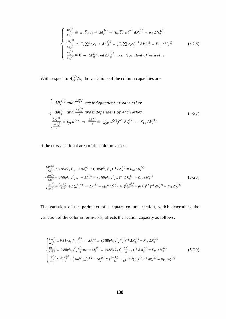
138
𝛥𝑁𝑢 𝑐
𝛥𝐴𝑠𝑙 𝑐 ≅ 𝐸𝑠 휀𝑖
𝑛𝑖 → 𝛥𝐴𝑠𝑙
𝑐 = (𝐸𝑠 휀𝑖
𝑛𝑖 )
−1 𝛥𝑁𝑢
𝑐 = 𝐾9 𝛥𝑁𝑢 𝑐
𝛥𝑀𝑢 𝐶
𝛥𝐴𝑠𝑙 𝑐 ≅ 𝐸𝑠 휀𝑖𝑒𝑖
𝑛𝑖 → 𝛥𝐴𝑠𝑙
𝑐 = (𝐸𝑠 휀𝑖𝑒𝑖
𝑛𝑖 )
−1 𝛥𝑀𝑢
𝑐 = 𝐾10 𝛥𝑀𝑢 𝑐
∆𝑉𝑢(𝑐)
𝛥𝐴𝑠𝑙 𝑐 ≅ 0 → ∆𝑉𝑢
(𝑐) 𝑎𝑛𝑑 𝛥𝐴𝑠𝑙
𝑐 𝑎𝑟𝑒 𝑖𝑛𝑑𝑒𝑝𝑒𝑛𝑑𝑒𝑛𝑡 𝑜𝑓 𝑒𝑎𝑐 𝑜𝑡𝑒𝑟
(5-26)
With respect to 𝐴𝑠𝑣(𝑐)
/𝑠, the variations of the column capacities are
𝛥𝑁𝑢
𝑐 𝑎𝑛𝑑
𝛥𝐴𝑠𝑣 𝑐
𝑠 𝑎𝑟𝑒 𝑖𝑛𝑑𝑒𝑝𝑒𝑛𝑑𝑒𝑛𝑡 𝑜𝑓 𝑒𝑎𝑐 𝑜𝑡𝑒𝑟
𝛥𝑀𝑢 𝑐
𝑎𝑛𝑑 𝛥𝐴𝑠𝑣
𝑐
𝑠 𝑎𝑟𝑒 𝑖𝑛𝑑𝑒𝑝𝑒𝑛𝑑𝑒𝑛𝑡 𝑜𝑓 𝑒𝑎𝑐 𝑜𝑡𝑒𝑟
∆𝑉𝑢(𝑐)
𝛥𝐴𝑠𝑣 𝑐
𝑠
≅ 𝑓𝑦𝑣𝑑(𝑐) → 𝛥𝐴𝑠𝑣
𝑐
𝑠≅ (𝑓𝑦𝑣 𝑑(𝑐))−1 ∆𝑉𝑢
(𝑏)= 𝐾11 ∆𝑉𝑢
(𝑏)
(5-27)
If the cross sectional area of the column varies:
𝛥𝑁𝑢 𝑐
∆𝐴𝑐(𝑐) ≅ 0.85𝛾𝑘𝑢 𝑓
′𝑐
→ ∆𝐴𝑐(𝑐)
≅ (0.85𝛾𝑘𝑢 𝑓′𝑐)−1 𝛥𝑁𝑢
𝑐 = 𝐾12 𝛥𝑁𝑢
𝑐
𝛥𝑀𝑢 𝑐
∆𝐴𝑐(𝑐) ≅ 0.85𝛾𝑘𝑢 𝑓
′𝑐𝑒𝑐 → ∆𝐴𝑐
(𝑐)≅ (0.85𝛾𝑘𝑢 𝑓
′𝑐𝑒𝑐)−1 𝛥𝑀𝑢
𝑐 = 𝐾13 𝛥𝑀𝑢
𝑐
∆𝑉𝑢(𝑐)
∆𝐴𝑐(𝑐) ≅
𝑓𝑦𝑣 𝐴𝑠𝑣 𝑐
2𝑠+ 𝛽(𝑓𝑐
′ )0.5 → ∆𝐴𝑐(𝑏)
= 𝛥((𝑐)𝑑(𝑐)) ≅ (𝑓𝑦𝑣 𝐴𝑠𝑣
𝑐
2𝑠+ 𝛽(𝑓𝑐
′ )0.5)−1 ∆𝑉𝑢 𝑐
= 𝐾14 ∆𝑉𝑢 𝑐
(5-28)
The variation of the perimeter of a square column section, which determines the
variation of the column formwork, affects the section capacity as follows:
𝛥𝑁𝑢 𝑐
∆𝑃𝑓(𝑐) ≅ 0.85𝛾𝑘𝑢 𝑓
′𝑐
𝑐
2 → ∆𝑃𝑓
(𝑐)≅ (0.85𝛾𝑘𝑢 𝑓
′𝑐
𝑐
2)−1 𝛥𝑁𝑢
𝑐 = 𝐾15 𝛥𝑁𝑢
𝑐
𝛥𝑀𝑢 𝑐
∆𝑃𝑓(𝑐) ≅ 0.85𝛾𝑘𝑢 𝑓
′𝑐
𝑐
2𝑒𝑐 → ∆𝑃𝑓
(𝑏)≅ (0.85𝛾𝑘𝑢 𝑓
′𝑐
𝑐
2 𝑒𝑐)−1 𝛥𝑀𝑢
𝑐 = 𝐾16 𝛥𝑀𝑢
𝑐
∆𝑉𝑢(𝑐)
∆𝑃𝑓(𝑐) ≅
𝑓𝑦𝑣 𝐴𝑠𝑣 𝑐
4𝑠+
1
2𝛽(𝑐)(𝑓𝑐
′ )0.5 → ∆𝑃𝑓(𝑐)
≅ (𝑓𝑦𝑣 𝐴𝑠𝑣
𝑐
4𝑠+
1
2𝛽(𝑐)(𝑓𝑐
′ )0.5)−1 𝛥𝑉𝑢 𝑐
= 𝐾17 𝛥𝑉𝑢 𝑐
(5-29)
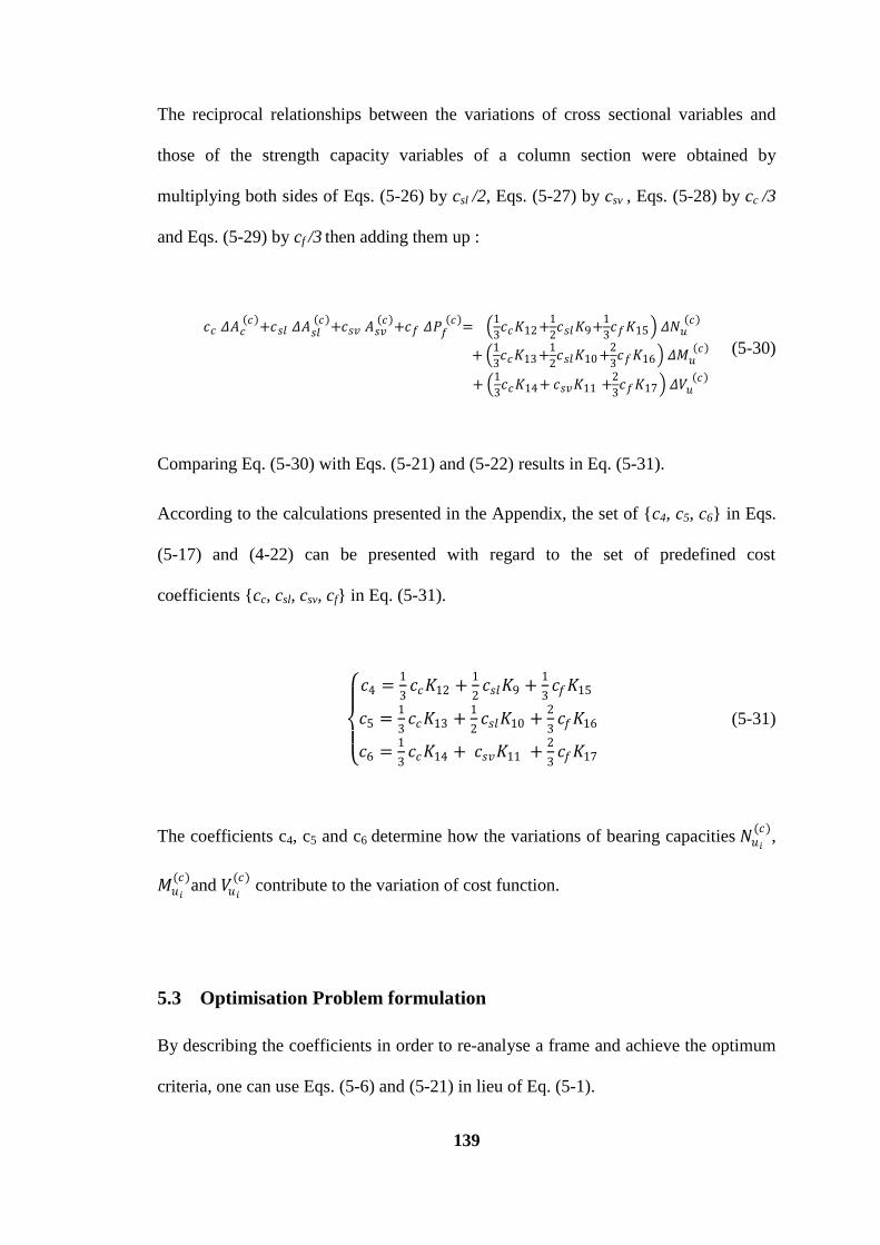
139
The reciprocal relationships between the variations of cross sectional variables and
those of the strength capacity variables of a column section were obtained by
multiplying both sides of Eqs. (5-26) by csl /2, Eqs. (5-27) by csv , Eqs. (5-28) by cc /3
and Eqs. (5-29) by cf /3 then adding them up :
𝑐𝑐 𝛥𝐴𝑐 𝑐
+𝑐𝑠𝑙 𝛥𝐴𝑠𝑙 𝑐
+𝑐𝑠𝑣 𝐴𝑠𝑣 𝑐
+𝑐𝑓 𝛥𝑃𝑓 𝑐
= 1
3𝑐𝑐𝐾12 +
1
2𝑐𝑠𝑙𝐾9+
1
3𝑐𝑓𝐾15 𝛥𝑁𝑢
𝑐
+
1
3𝑐𝑐𝐾13 +
1
2𝑐𝑠𝑙𝐾10 +
2
3𝑐𝑓𝐾16 𝛥𝑀𝑢
𝑐
+ 1
3𝑐𝑐𝐾14 + 𝑐𝑠𝑣𝐾11 +
2
3𝑐𝑓𝐾17 𝛥𝑉𝑢
𝑐
(5-30)
Comparing Eq. (5-30) with Eqs. (5-21) and (5-22) results in Eq. (5-31).
According to the calculations presented in the Appendix, the set of {c4, c5, c6} in Eqs.
(5-17) and (4-22) can be presented with regard to the set of predefined cost
coefficients {cc, csl, csv, cf} in Eq. (5-31).
𝑐4 =
1
3𝑐𝑐𝐾12 +
1
2𝑐𝑠𝑙𝐾9 +
1
3𝑐𝑓𝐾15
𝑐5 =1
3𝑐𝑐𝐾13 +
1
2𝑐𝑠𝑙𝐾10 +
2
3𝑐𝑓𝐾16
𝑐6 =1
3𝑐𝑐𝐾14 + 𝑐𝑠𝑣𝐾11 +
2
3𝑐𝑓𝐾17
(5-31)
The coefficients c4, c5 and c6 determine how the variations of bearing capacities 𝑁𝑢𝑖
(𝑐),
𝑀𝑢𝑖
(𝑐)and 𝑉𝑢𝑖
(𝑐) contribute to the variation of cost function.
5.3 Optimisation Problem formulation
By describing the coefficients in order to re-analyse a frame and achieve the optimum
criteria, one can use Eqs. (5-6) and (5-21) in lieu of Eq. (5-1).
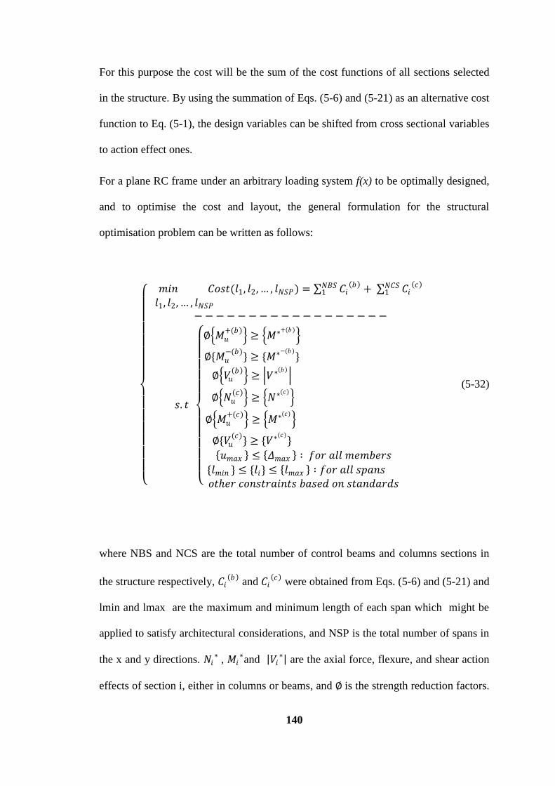
140
For this purpose the cost will be the sum of the cost functions of all sections selected
in the structure. By using the summation of Eqs. (5-6) and (5-21) as an alternative cost
function to Eq. (5-1), the design variables can be shifted from cross sectional variables
to action effect ones.
For a plane RC frame under an arbitrary loading system f(x) to be optimally designed,
and to optimise the cost and layout, the general formulation for the structural
optimisation problem can be written as follows:
𝑚𝑖𝑛 𝐶𝑜𝑠𝑡(𝑙1, 𝑙2, … , 𝑙𝑁𝑆𝑃) = 𝐶𝑖
𝑏 𝑁𝐵𝑆1 + 𝐶𝑖
𝑐 𝑁𝐶𝑆1
𝑙1, 𝑙2, … , 𝑙𝑁𝑆𝑃 − − − − − − − − − − − − − − − − − −
𝑠. 𝑡
∅ 𝑀𝑢+(𝑏)
≥ 𝑀∗+(𝑏)
∅{𝑀𝑢−(𝑏)
} ≥ {𝑀∗−(𝑏)}
∅ 𝑉𝑢 𝑏
≥ 𝑉∗ 𝑏
∅ 𝑁𝑢(𝑐)
≥ 𝑁∗(𝑐)
∅ 𝑀𝑢+(𝑐)
≥ 𝑀∗(𝑐)
∅{𝑉𝑢(𝑐)
} ≥ {𝑉∗(𝑐)}
𝑢𝑚𝑎𝑥 ≤ 𝛥𝑚𝑎𝑥 ∶ 𝑓𝑜𝑟 𝑎𝑙𝑙 𝑚𝑒𝑚𝑏𝑒𝑟𝑠
{𝑙𝑚𝑖𝑛 } ≤ {𝑙𝑖} ≤ 𝑙𝑚𝑎𝑥 ∶ 𝑓𝑜𝑟 𝑎𝑙𝑙 𝑠𝑝𝑎𝑛𝑠 𝑜𝑡𝑒𝑟 𝑐𝑜𝑛𝑠𝑡𝑟𝑎𝑖𝑛𝑡𝑠 𝑏𝑎𝑠𝑒𝑑 𝑜𝑛 𝑠𝑡𝑎𝑛𝑑𝑎𝑟𝑑𝑠
(5-32)
where NBS and NCS are the total number of control beams and columns sections in
the structure respectively, 𝐶𝑖 𝑏
and 𝐶𝑖 𝑐
were obtained from Eqs. (5-6) and (5-21) and
lmin and lmax are the maximum and minimum length of each span which might be
applied to satisfy architectural considerations, and NSP is the total number of spans in
the x and y directions. 𝑁𝑖∗ , 𝑀𝑖
∗and 𝑉𝑖∗ are the axial force, flexure, and shear action
effects of section i, either in columns or beams, and ∅ is the strength reduction factors.
141
The serviceability requirements limit the maximum deflection umax on the entire
member to Δmax under the serviceability load case. Other constraints for durability,
fire resistance, minimum cover, and minimum flexural strength, can easily be added to
the problem as well, based on the relevant design codes.
There are several ways of dealing with the above cost optimisation problem. Although
the problem of finding the layout of a frame is a continuous optimisation problem, it
can be dealt with as a discreet problem by discretising the domain. In fact in the
design process we usually deal with the dimensions as discrete sizes, and in practical
problems it is often the case that design variables must be chosen within a discrete
manufacturer's inventory. The dimensions of concrete sections are usually varied by a
certain size, e.g. 25 mm or 50 mm a step, which makes the dimensions of a section
discrete. Therefore, one can define the optimisation problem of RC sections as a
discrete optimisation problem rather than a continuous one. In the next section, an Ant
Colony Algorithm is proposed as a discrete optimization tool to solve the problem.
5.4 ACO algorithm
Two main phases of the Ant System algorithm are the ants‘ solution construction and
the pheromone update. After defining the construction graph and the necessary
constraints, and specifying the magnitudes of the pheromone trails and heuristic
information for the problem, the ants start making the trails. Initially, the ants are put
on chosen nodes of the graph. At each construction step, Ant k applies a probabilistic
action choice rule, known as the random-proportional rule, to decide which node to
visit next. If an ant is positioned on a node it will move to the next node with a
probability that is proportional to the amount of pheromone in the trails. That is, the

142
probabilistic choice of the next node then works analogous to the roulette wheel
selection procedure of evolutionary computation. The quantity of pheromone trail and
heuristic value on the edges determines the size of the slice on a circular roulette
wheel. Obviously, the higher the pheromone or the higher the heuristic value on the
edges will increase the probability of selecting the corresponding node. After all the
ants have constructed their tours, the pheromone trails are updated. This act is done by
first lowering the pheromone value on all arcs by a constant factor (pheromone
evaporation), and then adding pheromone on the edges the ants have crossed
(pheromone depositing).
The aim of the ACO algorithm developed in this chapter was to find the optimum
layout or columns locations of a plane RC frame, which leads to finding the optimum
spans lengths of the frame, as shown in Fig. 5-2, in a way that optimises the relevant
costs. The heights of stories (columns heights) are considered to be determinate and
unchanging.
As a first step the domain must be discretised. As such aconstruction graph was
defined by assuming that that span lengths were bounded in [Lmin Lmax], with intervals
(accuracy) equal to ε. That is, each Li rests in the set of {Lmin , Lmin + ε, Lmin + 2ε ,…,
Lmax - ε , Lmax}. Obviously, the smaller ε is chosen, the more accurate will the results
be, and the more running time the algorithm needs. As shown in Fig. 5.2, a
construction graph was defined to demonstrate the possible span lengths of the 2D
frame. In order for the construction graph to stand for the layout of the structure, the
total number of spans and the number of nodes must be N and N+1 respectively,
where N is the total number of spans. Hence, the construction graph was defined as a
graph with N+1 nodes and ((Lmax -Lmin)/ ε *N) edges. Each pair of nodes are connected
with (Lmax - Lmin)/ ε edges, i.e. there are (Lmax - Lmin)/ ε choices for each ant on each
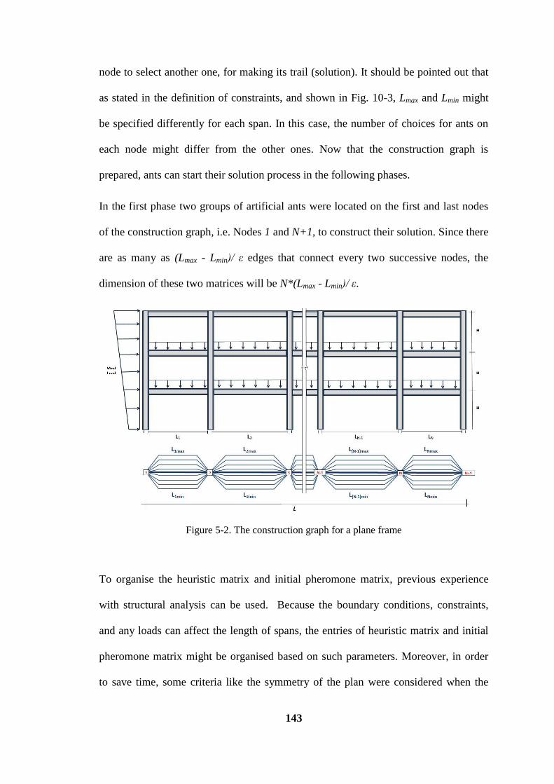
143
node to select another one, for making its trail (solution). It should be pointed out that
as stated in the definition of constraints, and shown in Fig. 10-3, Lmax and Lmin might
be specified differently for each span. In this case, the number of choices for ants on
each node might differ from the other ones. Now that the construction graph is
prepared, ants can start their solution process in the following phases.
In the first phase two groups of artificial ants were located on the first and last nodes
of the construction graph, i.e. Nodes 1 and N+1, to construct their solution. Since there
are as many as (Lmax - Lmin)/ ε edges that connect every two successive nodes, the
dimension of these two matrices will be N*(Lmax - Lmin)/ ε.
Figure 5-2. The construction graph for a plane frame
To organise the heuristic matrix and initial pheromone matrix, previous experience
with structural analysis can be used. Because the boundary conditions, constraints,
and any loads can affect the length of spans, the entries of heuristic matrix and initial
pheromone matrix might be organised based on such parameters. Moreover, in order
to save time, some criteria like the symmetry of the plan were considered when the
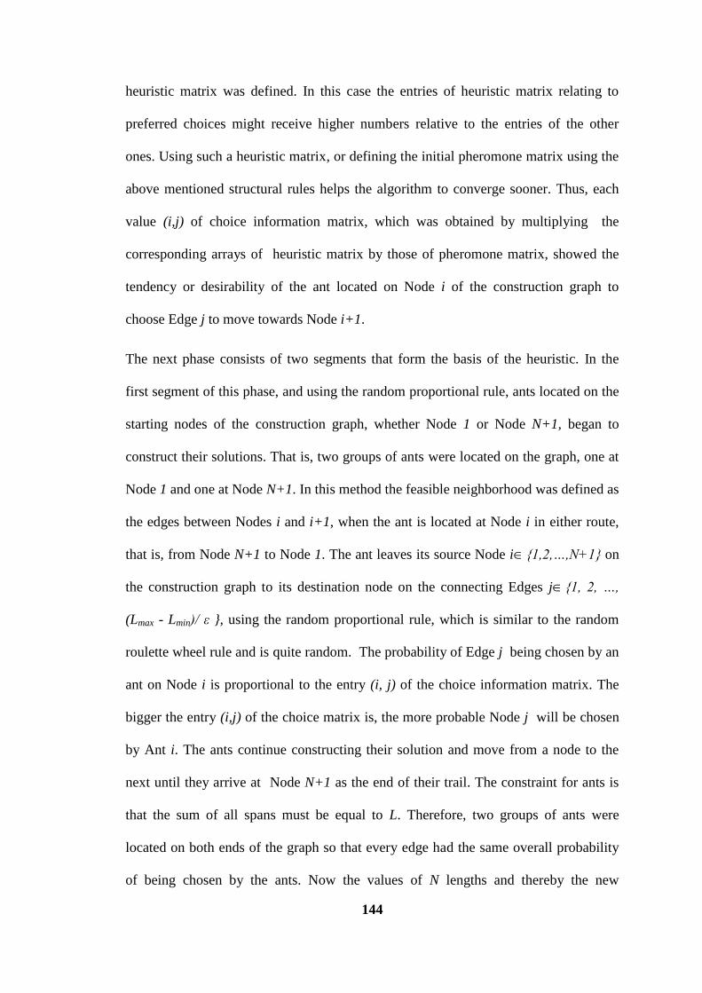
144
heuristic matrix was defined. In this case the entries of heuristic matrix relating to
preferred choices might receive higher numbers relative to the entries of the other
ones. Using such a heuristic matrix, or defining the initial pheromone matrix using the
above mentioned structural rules helps the algorithm to converge sooner. Thus, each
value (i,j) of choice information matrix, which was obtained by multiplying the
corresponding arrays of heuristic matrix by those of pheromone matrix, showed the
tendency or desirability of the ant located on Node i of the construction graph to
choose Edge j to move towards Node i+1.
The next phase consists of two segments that form the basis of the heuristic. In the
first segment of this phase, and using the random proportional rule, ants located on the
starting nodes of the construction graph, whether Node 1 or Node N+1, began to
construct their solutions. That is, two groups of ants were located on the graph, one at
Node 1 and one at Node N+1. In this method the feasible neighborhood was defined as
the edges between Nodes i and i+1, when the ant is located at Node i in either route,
that is, from Node N+1 to Node 1. The ant leaves its source Node i{1,2,…,N+1} on
the construction graph to its destination node on the connecting Edges j{1, 2, …,
(Lmax - Lmin)/ ε }, using the random proportional rule, which is similar to the random
roulette wheel rule and is quite random. The probability of Edge j being chosen by an
ant on Node i is proportional to the entry (i, j) of the choice information matrix. The
bigger the entry (i,j) of the choice matrix is, the more probable Node j will be chosen
by Ant i. The ants continue constructing their solution and move from a node to the
next until they arrive at Node N+1 as the end of their trail. The constraint for ants is
that the sum of all spans must be equal to L. Therefore, two groups of ants were
located on both ends of the graph so that every edge had the same overall probability
of being chosen by the ants. Now the values of N lengths and thereby the new
145
geometrical layout for the column layout was obtained. Through the structural analysis
method for frames, and using the behavioural constraints, design actions effects in the
sections identified were determined, and by using other constraints the required
strength capacities for each section were calculated. Based on the strength capacity of
sections, the cost function or the cost of this solution was obtained.
The last phase consisted of updating the information and statistics and then updating
the pheromone trails. Using the information obtained in the phase of constructing the
solution, the trail presenting the best cost up to this stage, was selected as the best
iteration so far. Then the pheromone trails of the construction graph were updated. For
this reason the ants were allowed to deposit pheromone on the edges associated with
the best so-far iteration and the quality of the solutions in each step. The process of
updating pheromone consists of two segments; the first segment corresponds to
pheromone evaporation where the evaporation parameter depends on the number of
steps defined for termination criteria, and initial pheromone and heuristic values; while
the second segment is depositing pheromone where the pheromone values on the
edges associated with the best iteration up to now increased and the ant deposited an
amount of pheromone equal to 1/cost on the edges of the construction graph associated
with the best so-far iteration and the cost of each solution.
The above procedure continues until the termination criterion has been satisfied,a nd
then the optimum layout will be the best-so-far solution for spans. In each step, a basic
structural analysis was required to calculate the section actions. By making use of a
structural analysis approach, say the finite element method or simplified methods
based on the design standards, such a calculation takes a small amount of time for each
section. Using Eq. (5-1) as the objective function would be significantly more time
consuming than using Eqs. (5-6) and (5-21). Due to the variation of lengths in each
146
step, estimating the design variables in each step would be considerably encumbered,
apart from which, in each step the algorithm would iteratively need to deal with the
design formulas. Eqs. (5-6) and (5-21) make the optimisation process much tangible
and greatly usable in optimising the layout of large structures.
5.5 Numerical example
To demonstrate the robustness of the proposed approach, a realistic example is
presented. All computations were performed on a P9700 @2.80 GHz computer
running MATLAB R2009b. In order to ensure that the solution obtained from ACO
was global or near global optimum, many runs were made in parallel. Since each run
is fully independent of the others, the program can be run in parallel so that the total
execution time will be practically the same as required for a single run.
Example: The column layout of a five-span eight-storey East-West oriented reinforced
concrete frame of a building located in Wollongong on a 20 m hill, as shown in Fig. 5-
3, was optimised. The building is 24.0 m high (each story 3.0 m high). The live load
and the total dead load are 5.0 and 4.0 kN/m2 respectively. The live load is 5.0 kN/m
2
and the dead load, excluding the self weight of concrete, is 2.5 kN/m2. The dynamic
effect of the wind loading was modelled by two windward and leeward impulse loads,
as shown in Fig. 5-3.
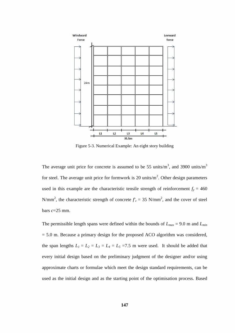
147
Figure 5-3. Numerical Example: An eight story building
The average unit price for concrete is assumed to be 55 units/m3, and 3900 units/m
3
for steel. The average unit price for formwork is 20 units/m2. Other design parameters
used in this example are the characteristic tensile strength of reinforcement fy = 460
N/mm2, the characteristic strength of concrete f'c = 35 N/mm
2, and the cover of steel
bars c=25 mm.
The permissible length spans were defined within the bounds of Lmax = 9.0 m and Lmin
= 5.0 m. Because a primary design for the proposed ACO algorithm was considered,
the span lengths L1 = L2 = L3 = L4 = L5 =7.5 m were used. It should be added that
every initial design based on the preliminary judgment of the designer and/or using
approximate charts or formulae which meet the design standard requirements, can be
used as the initial design and as the starting point of the optimisation process. Based
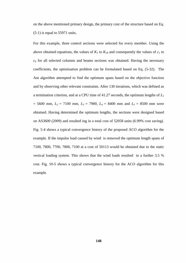
148
on the above mentioned primary design, the primary cost of the structure based on Eq.
(5-1) is equal to 55971 units.
For this example, three control sections were selected for every member. Using the
above obtained equations, the values of K1 to K18 and consequently the values of c1 to
c6 for all selected columns and beams sections was obtained. Having the necessary
coefficients, the optimisation problem can be formulated based on Eq. (5-32). The
Ant algorithm attempted to find the optimum spans based on the objective function
and by observing other relevant constraints. After 130 iterations, which was defined as
a termination criterion, and at a CPU time of 41.27 seconds, the optimum lengths of L1
= 5600 mm, L2 = 7100 mm, L3 = 7900, L4 = 8400 mm and L5 = 8500 mm were
obtained. Having determined the optimum lengths, the sections were designed based
on AS3600 (2009) and resulted ing in a total cost of 52058 units (6.99% cost saving).
Fig. 5-4 shows a typical convergence history of the proposed ACO algorithm for the
example. If the impulse load caused by wind is removed the optimum length spans of
7100, 7800, 7700, 7800, 7100 at a cost of 50113 would be obtained due to the static
vertical loading system. This shows that the wind loads resulted in a further 3.5 %
cost. Fig. 10-5 shows a typical convergence history for the ACO algorithm for this
example.
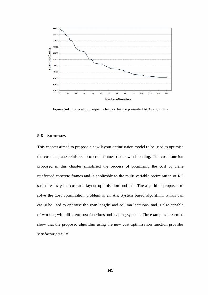
149
Figure 5-4. Typical convergence history for the presented ACO algorithm
5.6 Summary
This chapter aimed to propose a new layout optimisation model to be used to optimise
the cost of plane reinforced concrete frames under wind loading. The cost function
proposed in this chapter simplified the process of optimising the cost of plane
reinforced concrete frames and is applicable to the multi-variable optimisation of RC
structures; say the cost and layout optimisation problem. The algorithm proposed to
solve the cost optimisation problem is an Ant System based algorithm, which can
easily be used to optimise the span lengths and column locations, and is also capable
of working with different cost functions and loading systems. The examples presented
show that the proposed algorithm using the new cost optimisation function provides
satisfactory results.
150
6 Optimum Layout Design of RC Buildings with
Rectangular Plan
6.1 Introduction
This chapter presents the application of the methodology for optimising the cost of the
preliminary layout design of three-dimensional reinforced concrete (RC) frames with a
rectangular plan under static loads. This approach can easily be used for the optimal
layout design of a realistic and large RC structure that accounts for constraints
imposed by design standards. This approach considers modelling, structural analysis,
the design of concrete members, and discrete optimization, together with data on the
cost of systems and materials. The methodology consists of first, using the cross
sectional action effects as design variables where a heuristic cost function is presented
as an alternative to traditional cost functions for optimising the layout of RC
structures. Using the presented cost function, a structural optimisation problem is
formulated for a column layout design of 3D RC frames having a rectangular plan.
Then, an Ant System (AS) algorithm, a discrete method, was proposed to solve the
cost optimisation problem. Two comparative design examples are included to
151
demonstrate the performance of the new methodology and the excellent convergence
of the Ant Colony Optimization (ACO) algorithm.
In Chapters 4 and 5, it was noted that the process of achieving an optimum solution
can be much quicker by shifting from one design space to another and by changing the
design variables as the space dimensions. That is, shifting from one set of design
variables to another causes a new definition for the objective function and may lead to
changes in constraints and even vary their nature from design variables to behavioural
ones and vice versa.
In RC frames, at least three different cost factors should be considered in optimisation:
costs of concrete, steel reinforcement, and the formwork. The effects of these factors
on the optimal cost can be imposed on the weighted coefficients of the cost function,
so the general cost function for a reinforced concrete member can be expressed by Eq.
(4.2).
Using structural analytical outputs as design variables, say the internal actions of a
member, has some advantages over using structural design outcomes such as the cross
sectional variables of a beam. Firstly, the design action effects of each section can
easily be obtained from structural analysis and re-analysing a structure in an iterative
mathematical procedure is considerably less time consuming and more precise than
re-designing the structure. Secondly, the cost function using action effects will be
considered in a section rather than a member because it enables the designer to select
a number of sections for each member and control the cost in the whole structure, so
there is no need to optimise the entire member.
The present work explores the relationships between the variations of the action
effects of RC members with variations of the cross sectional parameters to establish
152
how these two variables affect each other. Based on the established relationship, a new
cost function which is a function of the action effects rather than the cross sectional
parameters has been defined. In order to make the structural optimisation formulation
practical and impose actual constraints, the formulation is based on the Australian
standards for RC structures (AS3600 2009).
In a 3D frame consisting of beams and columns the cost function can be written as Eq.
(5.1), where the superscript (c) stands for the column parameters and the superscript
(b) for beams, and where Nc and Nb are the number of columns and beams in the frame
respectively. In most published studies, the cost optimisation functions only deal with
cross sectional variables, whereas in the layout design of structures the cross sectional
variables are functions of the design action effects which are not determinate and vary
as the shape changes. Therefore, in an iterative procedure to solve an optimisation
problem, each step includes dealing with the structural analysis and structural design
variables. In such cases, unless alternative design variables are selected for the cost
function, the optimisation procedure might be too unwieldy. This situation holds as
long as parameters such as the cross sectional variables are obtained primarily from
implicit functions of structural analysis outputs based on the suggested relationships
and constraints in the design standards. On the other hand, design standards do not
uniquely provide the exact values for these cross sectional parameters and neithe are
they obtained from an explicit mathematical procedure.
As mentioned previously, in a layout optimisation problem, in addition to the classic
cross sectional variables, the layout of a structure would be variables of the problem. If
the reciprocal relationships between the cross sectional design factors and the design
action effects are determined, the cost can be represented as a function of the design
action effects. In the design process, having the design action effects in critical
153
sections such as all the crosssectional parameters, means that the total cost can be
calculated. Put simply, using the structural analysis outputs as design variables, such
as the internal actions of a member, has advantages over using structural design
outcomes such as the cross sectional characteristics of a beam. Firstly, the design
action effects of each section can easily be obtained from structural analysis, and in an
iterative mathematical procedure, re-analysing a structure is considerably less time
consuming and more precise than re-designing the structure. Moreover, by using
action effects the cost function will be considered in a section rather than a member,
which enables the designer to select a number of sections for each member and
control the cost in the whole structure, so there is no need to optimise the entire
member.
Therefore the aim of this chapter was to explore the relationship between the
variations of the action effects of RC members with the variations of the cross
sectional parameters to determine how these variables affect each other. Then, based
on such relationships, a new cost function that is a function of the action effects rather
than the cross sectional parameters was derived. In order to formulate the structural
optimisation problem, this study makes use of the requirements specified in the
Australian standard for concrete structures AS3600 (2009), which is based on the
limited state design method of concrete structures. A formulation for frames was
conducted separately on two groups of structural elements, namely beams and
columns.
154
6.2 Mathematical formulation
To design a beam, three action effects must be considered; the positive bending
moment, the negative bending moment, and the shear forces. If an arbitrary section of
a rectangular reinforced concrete beam, as shown in Fig. 10-1, is considered, the
dimensions of the section are b and h(b)
, the areas of tension and compression
reinforcement steel are 𝐴𝑠𝑡(𝑏)
, 𝐴𝑠𝑐(𝑏)
and the area of shear reinforcement steel in a unit
length of beam is 𝐴𝑠𝑣(𝑏)
/𝑠.
Consider Eq. (5-6) as a potential alternative cost functions to Eq. (5-1.1) in an
arbitrary RC beam section. The capacity or the ultimate strength of the section in
negative and positive flexure and shear for section i are 𝑀𝑢𝑖
− (𝑏) , 𝑀𝑢𝑖
+ (𝑏) and 𝑉𝑢𝑖
(𝑏)
respectively.
As mentoned in Capter 5, in order to shift from Eq. (5-1) and come up with the set of
{c1, c2, c3}, the first step is to determine how variations of 𝐴𝑐 𝑏
, 𝐴𝑠𝑙 𝑏
, 𝐴𝑠𝑣 𝑏
and
𝑃𝑓 𝑏
affect 𝑀𝑢+ (𝑏)
, 𝑀𝑢− (𝑏)
and 𝑉𝑢(𝑏)
, and vice versa. That is, the reciprocal relationships
between these two sets of variables must be identified to determine how increasing or
decreasing the amount of each cross sectional feature influences the section strength
capacities and how one should change the cross sectional parameters to vary the
section capacities. Given the unit costs cc, csl, csv and cf , the cost function can be
defined using Eq. (5-1.1) for each section of a beam. The parameters 𝐴𝑐 𝑏
, 𝐴𝑠𝑙 𝑏
, 𝐴𝑠𝑣 𝑏
and 𝑃𝑓 𝑏
were obtained from the sum of the cross sectional variables for all beams. If
any of the cross sectional parameters change the cost function varies, as shown in Eq.
(5.5). Eqs. (5-5) shows the contribution of each factor to the cost changes and the
sensitivity of cost to each term. For example, changing a unit of 𝐴𝑐 𝑏
caused a change
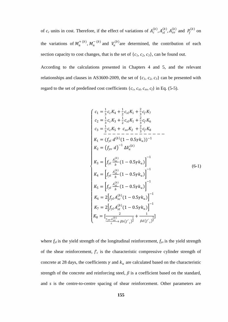
155
of cc units in cost. Therefore, if the effect of variations of 𝐴𝑐 𝑏
, 𝐴𝑠𝑙 𝑏
, 𝐴𝑠𝑣 𝑏
and 𝑃𝑓 𝑏
on
the variations of 𝑀𝑢+ (𝑏)
, 𝑀𝑢− (𝑏)
and 𝑉𝑢(𝑏)
are determined, the contribution of each
section capacity to cost changes, that is the set of {c1, c2, c3}, can be found out.
According to the calculations presented in Chapters 4 and 5, and the relevant
relationships and clauses in AS3600-2009, the set of {c1, c2, c3} can be presented with
regard to the set of predefined cost coefficients {cc, csl, csv, cf} in Eq. (5-5).
𝑐1 =
1
3𝑐𝑐𝐾4 +
1
2𝑐𝑠𝑙𝐾1 +
2
3𝑐𝑓𝐾7
𝑐2 =1
3𝑐𝑐𝐾3 +
1
2𝑐𝑠𝑙𝐾1 +
2
3𝑐𝑓𝐾6
𝑐3 =1
3𝑐𝑐𝐾5 + 𝑐𝑠𝑣𝐾2 +
2
3𝑐𝑓𝐾8
− − − − − − − − − − − − − − 𝐾1 = (𝑓𝑦𝑙 𝑑
𝑏 (1 − 0.5𝛾𝑘𝑢))−1
𝐾2 = 𝑓𝑦𝑣 𝑑 −1
∆𝑉𝑢 𝑏
𝐾3 = 𝑓𝑦𝑙𝐴𝑠𝑐
(𝑏)
𝑏(1 − 0.5𝛾𝑘𝑢 )
−1
𝐾4 = 𝑓𝑦𝑙𝐴𝑠𝑡
𝑏
𝑏 1 − 0.5𝛾𝑘𝑢
−1
𝐾5 = 𝑓𝑦𝑙𝐴𝑠𝑡
𝑏
𝑏 1 − 0.5𝛾𝑘𝑢
−1
𝐾6 = 2 𝑓𝑦𝑙 𝐴𝑠𝑐(𝑏)
(1 − 0.5𝛾𝑘𝑢 ) −1
𝐾7 = 2 𝑓𝑦𝑙 𝐴𝑠𝑡(𝑏)
(1 − 0.5𝛾𝑘𝑢 ) −1
𝐾8 = [2
𝑓𝑦𝑣 𝐴𝑠𝑣 𝑏
𝑠+ 𝛽𝑏 𝑓 ′
𝑐 12
+1
𝛽𝑑 𝑓 ′𝑐
12
]
(6-1)
where fyl is the yield strength of the longitudinal reinforcement, fyv is the yield strength
of the shear reinforcement, f'c is the characteristic compressive cylinder strength of
concrete at 28 days, the coefficients 𝛾 and 𝑘𝑢 are calculated based on the characteristic
strength of the concrete and reinforcing steel, β is a coefficient based on the standard,
and s is the centre-to-centre spacing of shear reinforcement. Other parameters are
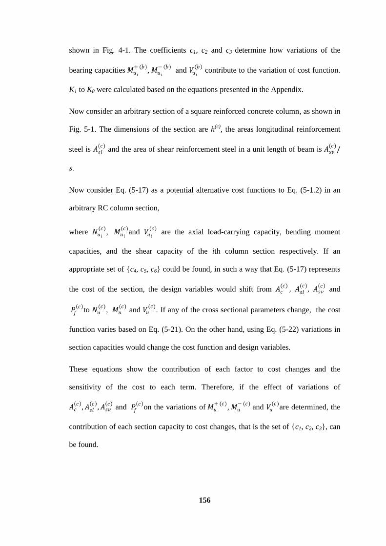
156
shown in Fig. 4-1. The coefficients c1, c2 and c3 determine how variations of the
bearing capacities 𝑀𝑢𝑖
+ (𝑏), 𝑀𝑢𝑖
− (𝑏) and 𝑉𝑢𝑖
(𝑏) contribute to the variation of cost function.
K1 to K8 were calculated based on the equations presented in the Appendix.
Now consider an arbitrary section of a square reinforced concrete column, as shown in
Fig. 5-1. The dimensions of the section are h(c)
, the areas longitudinal reinforcement
steel is 𝐴𝑠𝑙(𝑐)
and the area of shear reinforcement steel in a unit length of beam is 𝐴𝑠𝑣(𝑐)
/
𝑠.
Now consider Eq. (5-17) as a potential alternative cost functions to Eq. (5-1.2) in an
arbitrary RC column section,
where 𝑁𝑢𝑖
(𝑐), 𝑀𝑢𝑖
(𝑐)and 𝑉𝑢𝑖
(𝑐) are the axial load-carrying capacity, bending moment
capacities, and the shear capacity of the ith column section respectively. If an
appropriate set of {c4, c5, c6} could be found, in such a way that Eq. (5-17) represents
the cost of the section, the design variables would shift from 𝐴𝑐(𝑐)
, 𝐴𝑠𝑙(𝑐)
, 𝐴𝑠𝑣 𝑐
and
𝑃𝑓 𝑐
to 𝑁𝑢(𝑐)
, 𝑀𝑢(𝑐)
and 𝑉𝑢(𝑐)
. If any of the cross sectional parameters change, the cost
function varies based on Eq. (5-21). On the other hand, using Eq. (5-22) variations in
section capacities would change the cost function and design variables.
These equations show the contribution of each factor to cost changes and the
sensitivity of the cost to each term. Therefore, if the effect of variations of
𝐴𝑐 𝑐
, 𝐴𝑠𝑙 𝑐
, 𝐴𝑠𝑣 𝑐
and 𝑃𝑓 𝑐
on the variations of 𝑀𝑢+ (𝑐)
, 𝑀𝑢− (𝑐)
and 𝑉𝑢(𝑐)
are determined, the
contribution of each section capacity to cost changes, that is the set of {c1, c2, c3}, can
be found.
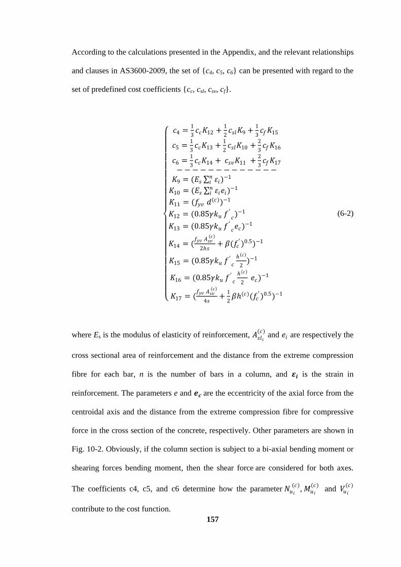
157
According to the calculations presented in the Appendix, and the relevant relationships
and clauses in AS3600-2009, the set of {c4, c5, c6} can be presented with regard to the
set of predefined cost coefficients {cc, csl, csv, cf}.
𝑐4 =
1
3𝑐𝑐𝐾12 +
1
2𝑐𝑠𝑙𝐾9 +
1
3𝑐𝑓𝐾15
𝑐5 =1
3𝑐𝑐𝐾13 +
1
2𝑐𝑠𝑙𝐾10 +
2
3𝑐𝑓𝐾16
𝑐6 =1
3𝑐𝑐𝐾14 + 𝑐𝑠𝑣𝐾11 +
2
3𝑐𝑓𝐾17
− − − − − − − − − − − − −𝐾9 = (𝐸𝑠 휀𝑖
𝑛𝑖 )−1
𝐾10 = (𝐸𝑠 휀𝑖𝑒𝑖𝑛𝑖 )−1
𝐾11 = (𝑓𝑦𝑣 𝑑(𝑐))−1
𝐾12 = (0.85𝛾𝑘𝑢 𝑓′𝑐)−1
𝐾13 = (0.85𝛾𝑘𝑢 𝑓′𝑐𝑒𝑐)−1
𝐾14 = (𝑓𝑦𝑣 𝐴𝑠𝑣
𝑐
2𝑠+ 𝛽(𝑓𝑐
′)0.5)−1
𝐾15 = (0.85𝛾𝑘𝑢 𝑓′𝑐
𝑐
2)−1
𝐾16 = (0.85𝛾𝑘𝑢 𝑓′𝑐
𝑐
2 𝑒𝑐)−1
𝐾17 = (𝑓𝑦𝑣 𝐴𝑠𝑣
𝑐
4𝑠+
1
2𝛽(𝑐)(𝑓𝑐
′)0.5)−1
(6-2)
where Es is the modulus of elasticity of reinforcement, 𝐴𝑠𝑙𝑖
(𝑐) and 𝑒𝑖 are respectively the
cross sectional area of reinforcement and the distance from the extreme compression
fibre for each bar, n is the number of bars in a column, and 𝜺𝒊 is the strain in
reinforcement. The parameters e and 𝒆𝒄 are the eccentricity of the axial force from the
centroidal axis and the distance from the extreme compression fibre for compressive
force in the cross section of the concrete, respectively. Other parameters are shown in
Fig. 10-2. Obviously, if the column section is subject to a bi-axial bending moment or
shearing forces bending moment, then the shear force are considered for both axes.
The coefficients c4, c5, and c6 determine how the parameter 𝑁𝑢𝑖
(𝑐), 𝑀𝑢𝑖
(𝑐) and 𝑉𝑢𝑖
(𝑐)
contribute to the cost function.
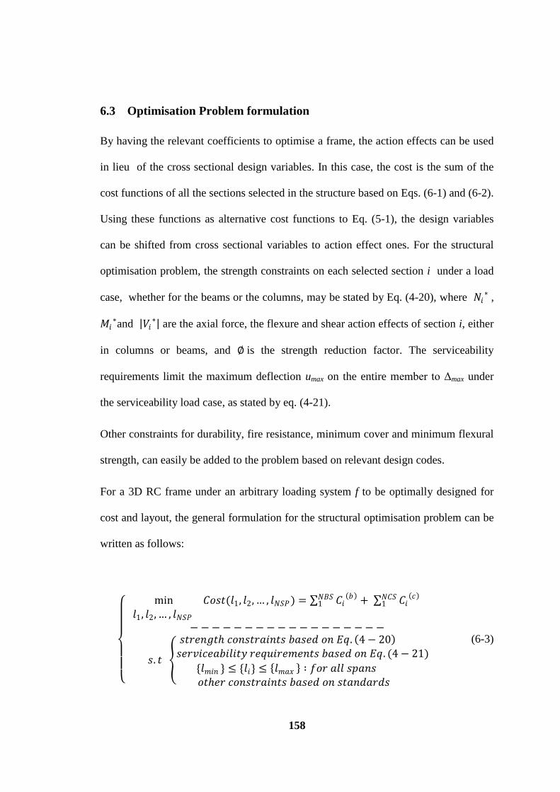
158
6.3 Optimisation Problem formulation
By having the relevant coefficients to optimise a frame, the action effects can be used
in lieu of the cross sectional design variables. In this case, the cost is the sum of the
cost functions of all the sections selected in the structure based on Eqs. (6-1) and (6-2).
Using these functions as alternative cost functions to Eq. (5-1), the design variables
can be shifted from cross sectional variables to action effect ones. For the structural
optimisation problem, the strength constraints on each selected section i under a load
case, whether for the beams or the columns, may be stated by Eq. (4-20), where 𝑁𝑖∗ ,
𝑀𝑖∗and 𝑉𝑖
∗ are the axial force, the flexure and shear action effects of section i, either
in columns or beams, and ∅ is the strength reduction factor. The serviceability
requirements limit the maximum deflection umax on the entire member to Δmax under
the serviceability load case, as stated by eq. (4-21).
Other constraints for durability, fire resistance, minimum cover and minimum flexural
strength, can easily be added to the problem based on relevant design codes.
For a 3D RC frame under an arbitrary loading system f to be optimally designed for
cost and layout, the general formulation for the structural optimisation problem can be
written as follows:
min 𝐶𝑜𝑠𝑡(𝑙1, 𝑙2, … , 𝑙𝑁𝑆𝑃) = 𝐶𝑖
𝑏 𝑁𝐵𝑆1 + 𝐶𝑖
𝑐 𝑁𝐶𝑆1
𝑙1, 𝑙2, … , 𝑙𝑁𝑆𝑃 − − − − − − − − − − − − − − − − − −
𝑠. 𝑡
𝑠𝑡𝑟𝑒𝑛𝑔𝑡 𝑐𝑜𝑛𝑠𝑡𝑟𝑎𝑖𝑛𝑡𝑠 𝑏𝑎𝑠𝑒𝑑 𝑜𝑛 𝐸𝑞. 4 − 20 𝑠𝑒𝑟𝑣𝑖𝑐𝑒𝑎𝑏𝑖𝑙𝑖𝑡𝑦 𝑟𝑒𝑞𝑢𝑖𝑟𝑒𝑚𝑒𝑛𝑡𝑠 𝑏𝑎𝑠𝑒𝑑 𝑜𝑛 𝐸𝑞. (4 − 21)
{𝑙𝑚𝑖𝑛 } ≤ {𝑙𝑖} ≤ 𝑙𝑚𝑎𝑥 ∶ 𝑓𝑜𝑟 𝑎𝑙𝑙 𝑠𝑝𝑎𝑛𝑠 𝑜𝑡𝑒𝑟 𝑐𝑜𝑛𝑠𝑡𝑟𝑎𝑖𝑛𝑡𝑠 𝑏𝑎𝑠𝑒𝑑 𝑜𝑛 𝑠𝑡𝑎𝑛𝑑𝑎𝑟𝑑𝑠
(6-3)
159
where NBS and NCS are the total number of control beams and column sections in the
structure respectively, 𝐶𝑖 𝑏
and 𝐶𝑖 𝑐
are obtained from Eqs. (6-1), and (6-2) and lmin
and lmax are the maximum and minimum lengths of each span which might be applied
in order to satisfy architectural considerations, and NSP is the total number of spans in
the x and y directions.
There are several ways to deal with the above cost optimisation problem. Although
optimising the layout of a frame is a continuous problem it can be dealt with as a
discrete problem by discretising the domain. In fact, in the design process we usually
deal with the dimensions as discrete sizes, but in practical problems design variables
must that are within a discrete manufacturer's inventory must often be chosen. The
dimensions of concrete sections are usually varied by a certain size, e.g. 25 mm or 50
mm a step, which makes the section dimensions discrete. Therefore, one can define the
optimisation problem of RC sections as a discrete optimisation problem rather than a
continuous one. In the next section an Ant Colony Algorithm has been proposed as a
discrete optimisation tool to solve the problem.
6.4 ACO algorithm
The aim of the ACO algorithm developed in this chapter was to find the optimum
column layout locations of a 3D RC frame with a rectangular plan, which leads to the
optimum spans of the frame in both the x and y directions, as shown in Fig. 6-1, in a
way that optimises the relevant costs. The height of stories, that is column lengths, was
considered to be determinate and constant. The Ant System (AS), as the first ACO
algorithm, has been applied successfully to many combinatorial optimisation problems
over the past decade, indeed many of the present Ant Colony Optimisation (ACO)
160
algorithms are the extensions of the Ant System (AS) algorithm. Two main phases of
the AS algorithm are the construction of the ants‘ solution and the pheromone update.
As a first step the domain must be discretised. As such the construction graph was
defined by assuming that the span lengths are bounded in [Lmin Lmax] in either direction
(Lmin and Lmax might be different between the x and y direction) with intervals
(accuracy) equal to ε. That is, each Li rests in the set of {Lmin , Lmin + ε, Lmin + 2ε ,…,
Lmax - ε , Lmax}. Obviously, the smaller ε is, the more accurate the results will be and
the more running time the algorithm needs. As shown in Fig. 9-3, an L-shape graph
was defined as the construction graph to demonstrate the plan of the 3D frame in the
x-y plane. The members on the horizontal and vertical wings of the graph denote spans
in the x and y directions respectively. In order for the construction graph to stand for
the structural layout, the total number of spans and the number of nodes need to be
Nx+Ny and (Nx+Ny+1) respectively, and where Nx and Ny are the total number of spans
in the x and y directions respectively. Hence, the construction graph is defined as a
graph with Nx+Ny+1 nodes and ((Lmax -Lmin)/ ε *Nx)+((Lmax - Lmin)/ ε *Ny) edges. Each
pair of nodes are connected with (Lmax - Lmin)/ ε edges, i.e. there are (Lmax - Lmin)/ ε
choices for each ant on each node to select another one for making its trail (solution).
It should be pointed out that as stated in the definition of constraints, and shown in
Fig. 9-3, Lmax and Lmin might be specified differently for each span, but in this case the
number of choices for ants on each node might differ from the other ones. Now that
the construction graph has been prepared the ants can start their solution process in
the following phases (Kaveh and Sharafi 2008a).
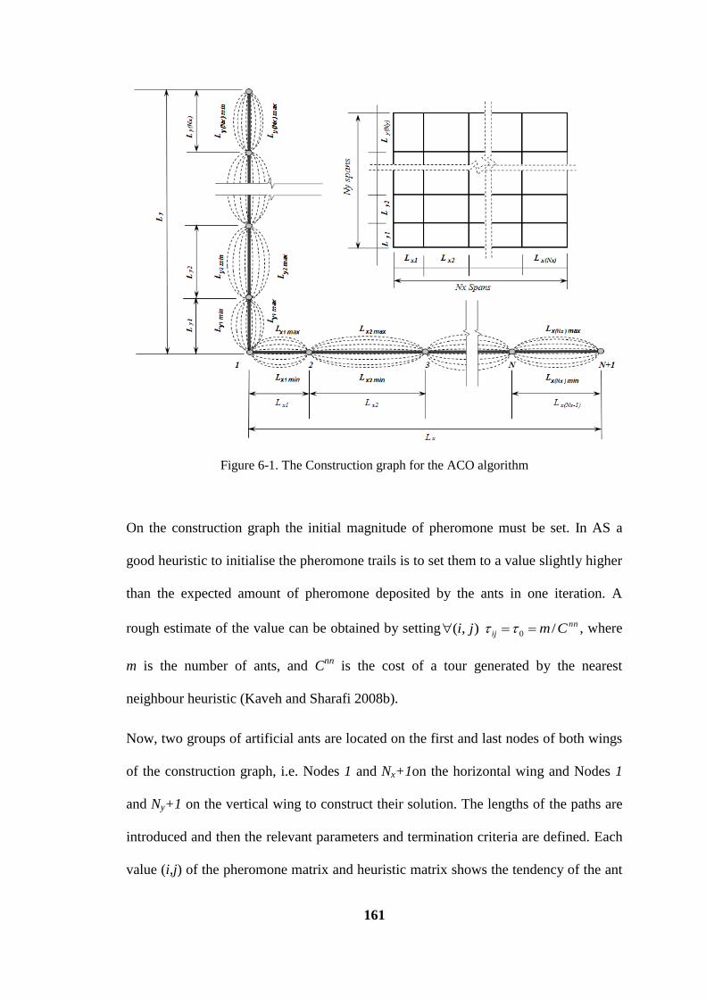
161
Figure 6-1. The Construction graph for the ACO algorithm
On the construction graph the initial magnitude of pheromone must be set. In AS a
good heuristic to initialise the pheromone trails is to set them to a value slightly higher
than the expected amount of pheromone deposited by the ants in one iteration. A
rough estimate of the value can be obtained by setting nn
ij Cmji / ),( 0 , where
m is the number of ants, and Cnn
is the cost of a tour generated by the nearest
neighbour heuristic (Kaveh and Sharafi 2008b).
Now, two groups of artificial ants are located on the first and last nodes of both wings
of the construction graph, i.e. Nodes 1 and Nx+1on the horizontal wing and Nodes 1
and Ny+1 on the vertical wing to construct their solution. The lengths of the paths are
introduced and then the relevant parameters and termination criteria are defined. Each
value (i,j) of the pheromone matrix and heuristic matrix shows the tendency of the ant
162
located on Node i of the construction graph to choose Edge j to move towards the next
node. Since there are as many as (Lmax - Lmin)/ ε edges that connect every two
successive nodes, the dimension of these two matrices will be (Ny+Nx)*(Lmax - Lmin)/ ε.
To organise the heuristic matrix and initial pheromone matrix, we can make use of our
experience with structural analysis; as as the boundary conditions, constraints, and
any loads can affect the length of the spans, the entries of the heuristic matrix and
initial pheromone matrix might be organised based on such parameters. Moreover, in
order to save time, some criteria like the symmetry of the plan were considered when
the heuristic matrix was defined. In this case the entries of heuristic matrix relating to
the preferred choices might receive higher numbers relative to the entries of the other
ones. Using such a heuristic matrix or defining the initial pheromone matrix using the
above mentioned structural rules helps the algorithm converge sooner. Thus each
value (i,j) of choice information matrix, which is obtained by multiplying the
corresponding arrays of heuristic matrix by those of the pheromone matrix, shows the
tendency or desirability of the ant located on Node i of the construction graph to
choose Edge j to move towards Node i+1.
The next phase consists of two segments that form the basis of the heuristic. In the
first segment of this phase, ants located on the starting nodes of the construction graph,
whether Node 1 or Node N+1 (N stands for Nx on the horizontal wing and for Ny on
the vertical one) on either wing, start to construct their solutions. At each construction
step, Ant k applies a probabilistic action choice rule based on Eq. (3-14), known as the
random-proportional rule, to decide which edge to visit next.
That is, the ant leaves its source Node i{1,2,…,N+1} on the construction graph and
proceeds to destination node on the connecting Edges j{1, 2, …, (Lmax - Lmin)/ ε },
163
using the random proportional rule, which is similar to the random roulette wheel rule.
The probability of Edge j being chosen by an ant on Node i is proportional to the entry
(i, j) of the choice information matrix. This relationship forms the basis of the AS
algorithm and shows that if Ant k is positioned on Node i, it will move to the next
Node j with the probability of ρijk. In this relationship, τij is the magnitude of
pheromone on the trails and ηij is the heuristic value. α and β are two parameters which
determine the relative influence of the pheromone trail and the heuristic information.
Nik is the feasible neighborhood of Ant k when at Node i, that is, the set of edges that
Ant k is allowed to choose as its next destination, and is decided depending on the
problem at hand. The probabilistic choice of the next edge then works analogously to
the roulette wheel selection procedure of evolutionary computation. The quantity of
pheromone trail and heuristic value on the edges determines the size of the slice on a
circular roulette wheel. Obviously, the higher the pheromone or higher heuristic value
on the edges increases the possibility of selecting the corresponding node. The ants
continue constructing their solution and move from one node to another until they
reach Node N+1 on both wings as the end of their trail. The constraint for ants on the
horizontal wing is that the sum of all spans must be equal to Lx, and for those on the
vertical wing, Ly. Therefore, two groups of ants are located on the ends of both wings
of the graph, so that every edge has the same overall probability of being chosen by
the ants.
After the segment of random choice, the values of Nx+Ny lengths and thereby the new
geometrical layout for the x-y plane was obtained. Based on the accuracy required for
the calculations, a number of control sections are set for each member (for example,
one at each member end and one at midspan) (Kaveh and Sharafi 2009). Through the
structural analysis method for frames, and using the behavioural constraints, the

164
design action effects in the identified control sections were determined and using other
constraints, the bearing capacities required for each control section were calculated.
Based on the bearing capacity of the control sections, the cost function or the cost of
this solution was obtained.
The last phase consists of updating the information and statistics, and then updating
the pheromone trails using the information obtained in the phase of constructing the
solution. The trail presenting the best cost, up to this stage, was selected as the best
iteration so far, and then the pheromone trails of the construction graph were updated.
This was done by first lowering the pheromone value on all the arcs (pheromone
evaporation), and then adding pheromone onto the edges the ants have crossed
(pheromone depositing). Pheromone evaporation is done by lowering the pheromone
value on all edges by a constant factor ρ according to Eq. (3-15). In this segment the
parameter depends on the number of steps defined for the termination criteria and
the initial pheromone and heuristic values. Depositing pheromone is then done by
increasing the pheromone value on all the edges. For this purpose, ants are allowed to
deposit pheromone on the edges associated with the best iteration so far, and the
quality of the solutions in each step according to Eq. (3.16) and (3.17).The value of Ck
was taken as the cost of the best trail or the best iteration and Tk was the set of suitable
solutions. For depositing pheromone, the pheromone values on the edges associated
with the best iteration up to now increased and the Ant deposited an amount of
pheromone equal to 1/cost on the edges of the construction graph associated with the
best iteration so far; where cost is the value of cost function obtained from best
iteration.
This procedure continues until the termination criterion has been satisfied, and then
the optimum layout will be the best-so-far solution for spans. In each step, a basic
165
structural analysis was needed to calculate the section actions. By making use of a
structural analysis approach, say the finite element method or the simplified methods
based on design standards, such a calculation takes a small amount of time for each
section. Using Eq. (5-1) as the objective function would be significantly more time-
consuming than using Eqs. (6-1) and (6-2), but when Eq. (5-1) was used, due to the
variation of lengths in each step, the estimation of design variables in each step was
considerably encumbered, apart from the fact that in each step the algorithm needed
to iteratively deal with the design formulas. Eqs. (6-1) and (6-2) make the optimisation
process more practicable when optimising the layout of large structures.
6.5 Numerical examples
Two examples were presented to demonstrate the robustness of the proposed
approach. All the computations were performed on P9700 @2.80 GHz computer
running MATLAB R2009b. In order to ensure that the solution was global or near
global optimum, many runs were made in parallel. Since each run was fully
independent of the others, the program can be run in parallel so that the total execution
time will be practically the same as required for a single run.
Example 1: The column layout of a four storey reinforced concrete frame building,
each 2.90 m high, and with a plan as shown in Fig. 6-2(a) was further optimised in the
present work. The live load was 5.0 kN/m2 and the dead load, excluding the self-
weight of the concrete, was 2.5 kN/m2. The average unit price for concrete was
assumed to be 55 units/m3, and 3900 units/m
3 for reinforcing steel. The average unit
price for formwork was 20 units/m2. Other design parameters used in this example are
the characteristic tensile strength of steel reinforcement fy = 460 N/mm2, the
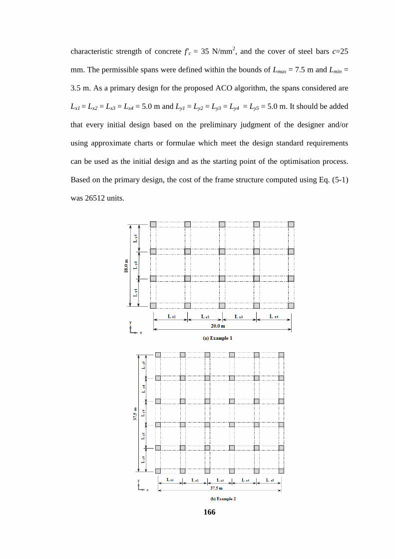
166
characteristic strength of concrete f'c = 35 N/mm2, and the cover of steel bars c=25
mm. The permissible spans were defined within the bounds of Lmax = 7.5 m and Lmin =
3.5 m. As a primary design for the proposed ACO algorithm, the spans considered are
Lx1 = Lx2 = Lx3 = Lx4 = 5.0 m and Ly1 = Ly2 = Ly3 = Ly4 = Ly5 = 5.0 m. It should be added
that every initial design based on the preliminary judgment of the designer and/or
using approximate charts or formulae which meet the design standard requirements
can be used as the initial design and as the starting point of the optimisation process.
Based on the primary design, the cost of the frame structure computed using Eq. (5-1)
was 26512 units.
167
Figure 6-2. Plane view of the primary design of the 3D frames
For this example, three control sections were selected for every member. Using the
above equations the values of K1 to K18, and consequently the values of c1 to c6 for all
selected columns and beams sections were obtained. Having the necessary
coefficients, the optimisation problem can be formulated based on Eq. (6-3).
The Ant algorithm attempted to find the optimum spans based on the objective
function and relevant constraints. After 105 iterations, and at a CPU time of 33.8
seconds, the optimum lengths of Lx1 = 4700 mm, Lx2 = 5300 mm, Lx3 = 5300 mm and
Lx4 = 4700 mm in the x direction, and Ly1 = 5800 mm, Ly2 = 6400 mm and Ly3 = 5800
mm in the y direction were obtained. Having determined the optimum lengths, the
sections were designed based on AS3600 (2009) resulting in a total cost of 25239
units.
The present methodology thus provided a further cost saving of 4.8% over the
previously optimised design of Sahab et al. (2005b). It should be noted that in Sahab's
work, the optimisation process was first carried out for a predefined shape and then the
optimum number of equal spans was obtained by using a genetic algorithm.
Example 2: Consider the plan of a three storey building as shown in Fig. 6-2(b). This
example was dealt with in a report on the comparative costs of concrete framed
buildings (Goodchild 1993) that were recommended as a benchmark for future studies.
A conventional design of this example was carried out and optimised by a team of
professional structural engineers. The total length and width of the building was 37.5
m and the heights of the storeys was 3.95 m. The live load on the intermediate floors
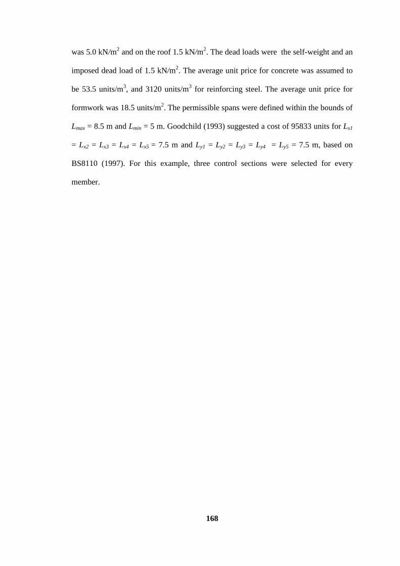
168
was 5.0 kN/m2 and on the roof 1.5 kN/m
2. The dead loads were the self-weight and an
imposed dead load of 1.5 kN/m2. The average unit price for concrete was assumed to
be 53.5 units/m3, and 3120 units/m
3 for reinforcing steel. The average unit price for
formwork was 18.5 units/m2. The permissible spans were defined within the bounds of
Lmax = 8.5 m and Lmin = 5 m. Goodchild (1993) suggested a cost of 95833 units for Lx1
= Lx2 = Lx3 = Lx4 = Lx5 = 7.5 m and Ly1 = Ly2 = Ly3 = Ly4 = Ly5 = 7.5 m, based on
BS8110 (1997). For this example, three control sections were selected for every
member.
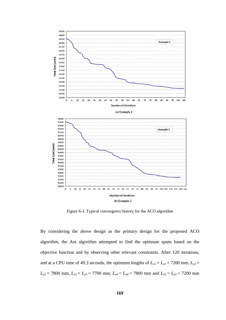
169
Figure 6-3. Typical convergence history for the ACO algorithm
By considering the above design as the primary design for the proposed ACO
algorithm, the Ant algorithm attempted to find the optimum spans based on the
objective function and by observing other relevant constraints. After 120 iterations,
and at a CPU time of 49.3 seconds, the optimum lengths of Lx1 = Ly1 = 7200 mm, Lx2 =
Ly2 = 7800 mm, Lx3 = Ly3 = 7700 mm, Lx4 = Ly4 = 7800 mm and Lx5 = Ly5 = 7200 mm
170
were obtained. Having determined the optimum lengths the sections were designed
based on AS3600 (2009) and this resulted in a total cost of 92568 units.
For both examples, the termination criterion for the ACO algorithms was defined as
the number of iterations when the improvement in the solution quality was less than
0.02% after ten consecutive iterations. Figs. 6-3(a) and 6-3(b) show typical
convergence histories of the proposed ACO algorithm for the examples.
6.6 Summary
This chapter presents a layout optimisation model for optimising the cost of a column
layout design of 3D reinforced concrete frames with a rectangular plan. The proposed
approach simplifies the optimisation process when the topology optimisation problem
considered the cost elements involved. The algorithm proposed for solving the cost
optimisation problem was an Ant System based algorithm that can easily be used to
optimise the span lengths and column locations and is also capable of working with
different cost functions. The examples presented show that the proposed algorithm
using the new cost optimisation function provided satisfactory results.
171
7 Optimum Layout Design of Rectangular Flat Plate Floor
Systems
7.1 Introduction
Flat plates are reinforced concrete floors resting directly onto columns without the use
of intermediary and drop panels, as shown in Fig. 7-1. These floors are conventionally
called flat slabs if they have drop panels around the column. The absence of beams
makes flat plate systems one of the most economical floor systems in terms of
construction, especially for medium and high rise buildings. They provide flexibility
for partition locations, they allow for easy fixing and passing services, simplified
formwork and architectural finishing, provid better fire resistance, less risk of concrete
spalling, and more importantly, greater vertical clearance for a given storey height.
These are the advantages of flat plate floor systems over other slab systems(Goodchild
1997; Fanella and Association 2000; Ashworth 2004; Goodchild et al. 2009).
A new preliminary layout optimisation methodology was proposed to optimise the
cost of buildings with a flat plate floor system. For this purpose, a heuristic cost
function is presented as an alternative to traditional objective functions. The
methodology and the new cost function have the potential of being easy to use when
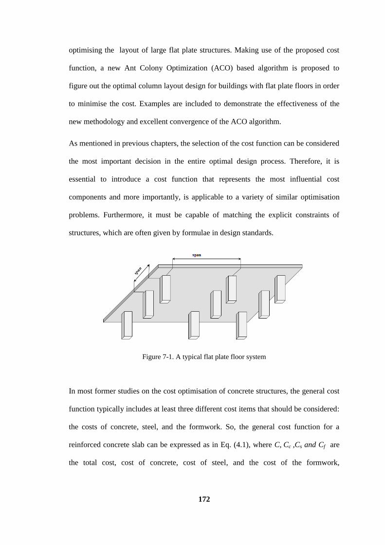
172
optimising the layout of large flat plate structures. Making use of the proposed cost
function, a new Ant Colony Optimization (ACO) based algorithm is proposed to
figure out the optimal column layout design for buildings with flat plate floors in order
to minimise the cost. Examples are included to demonstrate the effectiveness of the
new methodology and excellent convergence of the ACO algorithm.
As mentioned in previous chapters, the selection of the cost function can be considered
the most important decision in the entire optimal design process. Therefore, it is
essential to introduce a cost function that represents the most influential cost
components and more importantly, is applicable to a variety of similar optimisation
problems. Furthermore, it must be capable of matching the explicit constraints of
structures, which are often given by formulae in design standards.
Figure 7-1. A typical flat plate floor system
In most former studies on the cost optimisation of concrete structures, the general cost
function typically includes at least three different cost items that should be considered:
the costs of concrete, steel, and the formwork. So, the general cost function for a
reinforced concrete slab can be expressed as in Eq. (4.1), where C, Cc ,Cs and Cf are
the total cost, cost of concrete, cost of steel, and the cost of the formwork,
173
respectively. Obviously, for pre-stressed and fibred concrete sections the relevant costs
for these two items are added to the total cost.
By considering the unit costs per parameter, Eq. (4-1) can be written like Eq.(4-2),
where cc, cs, and cf are the unit costs of concrete, longitudinal steel, and the formwork
respectively, and Ac, As, and Pf are their corresponding quantities. The effects of the
cost of materials, transportation, fabrication, and even maintenance, in addition to the
cost of repairs and insurance, can be presented by such a weighted sum. The effect of
these factors on the optimal cost can be imposed on the weighted coefficients of the
cost function. In a building with a flat plate system that mainly consists of columns
and slabs, the cost can be written as follows:
𝐶 𝑠 = 𝑐𝑐𝐴𝑐
(𝑠) + 𝑐𝑠𝑙 𝐴𝑠
(𝑠)+ 𝑐𝑓 𝑃𝑓
𝑏 (7 − 1.1)
𝐶 𝑐 = 𝑐𝑐𝐴𝑐 𝑐
+ 𝑐𝑠𝑙 𝐴𝑠𝑙 𝑐
+ 𝑐𝑠𝑣 𝐴𝑠𝑣 𝑐
+ 𝑐𝑓 𝑃𝑓 𝑐
7 − 1.2
𝐶 = 𝐶 𝑠 𝑁𝑠1 + 𝐶 𝑐 𝑁𝑐
1 (7 − 1.3)
(7-1)
where the superscript (c) stands for the column parameters and the superscript (s) for
slabs, and Nc and Ns are the number of columns and slabs in the building respectively.
In most published optimisation studies in the field of flat slab floors which make use
of such a classic cost function for a RC structural optimisation problem, some or all of
the above mentioned parameters are considered to be the design variables. Then, based
on the explicit constraints presented in standards and/or implicit behavioural
constraints of the problem, the optimum values of the design variables will be found
using optimisation techniques. In other words, most current cost optimisation
functions deal only with cross sectional variables.
174
In case of topology or the layout optimisation of large structures where the shape or
the number or lengths of structural members are not predefined, using a formulation
that is currently available leads to a significant number of design variables and
constraints.
Furthermore, in order to determine the cross sectional parameters, the first step is to
complete the structural analysis procedure, and then use the structural analysis outputs
such as forces and bending moments together with the design standard requirements,
to determine the cross sectional characteristics of the concrete section. To put it
simply, using such an optimisation formulation means that each step of the cost
optimisation for the layout design of a structure includes both analysis and design
processes. In this case, besides the classic cross sectional variables, the layout
characteristics of a structure such as the lengths of spans in a multi-span structure,
would be variables of the problem, so the designer must repeat the design procedure to
achieve the optimal cross sectional variables that are usually functions of other layout
variables. That is why most published structural topology optimisation works focus on
minimising the weight rather than the cost of structures.
As was performed in sections 4 to 6, if the reciprocal relationships between the cross
sectional design factors and the design action effects are determined, the cost can be
represented as a function of the design action effects. In the design process the design
action effects are determined for the critical sections of members and then the cross
sectional variables are calculated for each section. Cross sectional parameters along
the structural members are obtained from the critical sections based on the
requirements of the design standards. In fact, having the design action effects in
critical sections means that all the cross sectional parameters and the total cost based
on Eq. (4-2) can be calculated. To put it simply, using structural analysis outputs of
175
theinternal actions of a member as design variables for example, has advantages over
using structural design outcomes such as the cross sectional characteristics of a beam.
Firstly, the design action effects of each section can easily be obtained from structural
analysis, and in an iterative mathematical procedure, re-analysing a structure is
considerably less time consuming and more precise than re-designing the structure.
Moreover, by using action effects the cost function will be considered in a section
rather than a member. This enables the designer to select a number of sections for each
member and to control the cost in the whole structure, so there is no need to optimise
the entire member.
Therefore, the aim of this section is to explore the relationship between the variations
of action effects of RC members in flat slab floors with the variations of the cross
sectional parameters and determine how these two types of variables affect each other.
Then, based on such relationships, a new cost function is derived that is a function of
the action effects rather than the cross sectional parameters.
7.2 Mathematical formulation
In order to formulate the structural optimisation problem for flat plate floors, this study
made use of the requirements specified in the Australian standard for concrete
structures (AS3600 2009), which is based on the limited state design method of
concrete structures. The frames consist of two groups of structural elements: beams
and columns; which have key roles in the total cost of a frame.
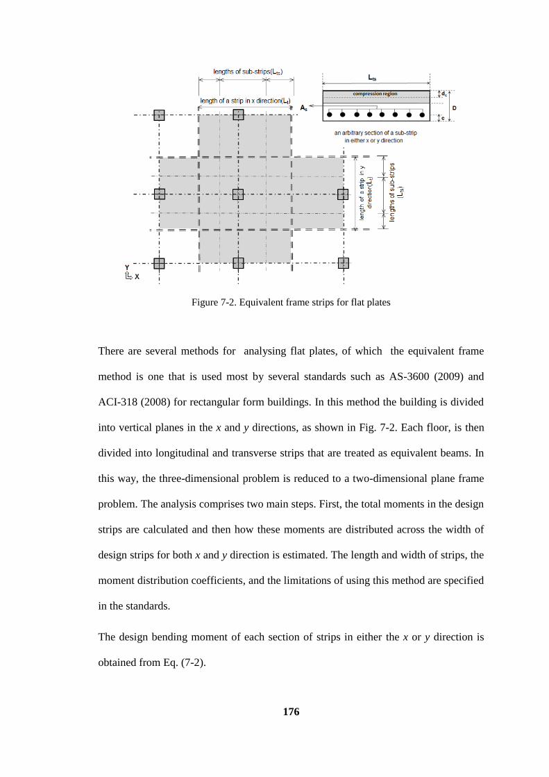
176
Figure 7-2. Equivalent frame strips for flat plates
There are several methods for analysing flat plates, of which the equivalent frame
method is one that is used most by several standards such as AS-3600 (2009) and
ACI-318 (2008) for rectangular form buildings. In this method the building is divided
into vertical planes in the x and y directions, as shown in Fig. 7-2. Each floor, is then
divided into longitudinal and transverse strips that are treated as equivalent beams. In
this way, the three-dimensional problem is reduced to a two-dimensional plane frame
problem. The analysis comprises two main steps. First, the total moments in the design
strips are calculated and then how these moments are distributed across the width of
design strips for both x and y direction is estimated. The length and width of strips, the
moment distribution coefficients, and the limitations of using this method are specified
in the standards.
The design bending moment of each section of strips in either the x or y direction is
obtained from Eq. (7-2).
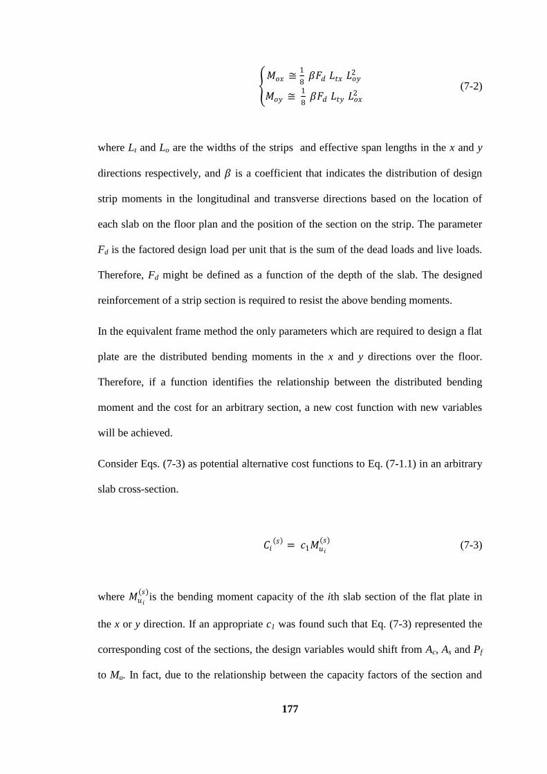
177
𝑀𝑜𝑥 ≅
1
8 𝛽𝐹𝑑 𝐿𝑡𝑥 𝐿𝑜𝑦
2
𝑀𝑜𝑦 ≅ 1
8 𝛽𝐹𝑑 𝐿𝑡𝑦 𝐿𝑜𝑥
2 (7-2)
where Lt and Lo are the widths of the strips and effective span lengths in the x and y
directions respectively, and 𝛽 is a coefficient that indicates the distribution of design
strip moments in the longitudinal and transverse directions based on the location of
each slab on the floor plan and the position of the section on the strip. The parameter
Fd is the factored design load per unit that is the sum of the dead loads and live loads.
Therefore, Fd might be defined as a function of the depth of the slab. The designed
reinforcement of a strip section is required to resist the above bending moments.
In the equivalent frame method the only parameters which are required to design a flat
plate are the distributed bending moments in the x and y directions over the floor.
Therefore, if a function identifies the relationship between the distributed bending
moment and the cost for an arbitrary section, a new cost function with new variables
will be achieved.
Consider Eqs. (7-3) as potential alternative cost functions to Eq. (7-1.1) in an arbitrary
slab cross-section.
𝐶𝑖 𝑠 = 𝑐1𝑀𝑢𝑖
(𝑠) (7-3)
where 𝑀𝑢𝑖
(𝑠)is the bending moment capacity of the ith slab section of the flat plate in
the x or y direction. If an appropriate c1 was found such that Eq. (7-3) represented the
corresponding cost of the sections, the design variables would shift from Ac, As and Pf
to Mu. In fact, due to the relationship between the capacity factors of the section and
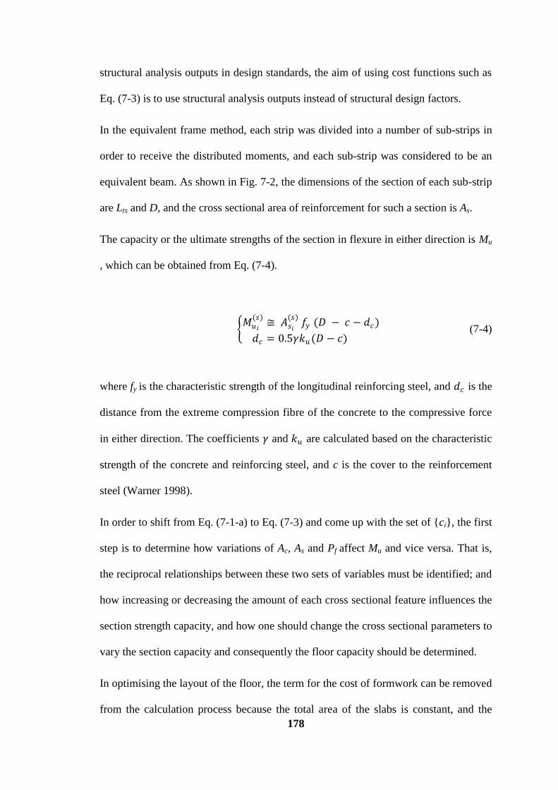
178
structural analysis outputs in design standards, the aim of using cost functions such as
Eq. (7-3) is to use structural analysis outputs instead of structural design factors.
In the equivalent frame method, each strip was divided into a number of sub-strips in
order to receive the distributed moments, and each sub-strip was considered to be an
equivalent beam. As shown in Fig. 7-2, the dimensions of the section of each sub-strip
are Lts and D, and the cross sectional area of reinforcement for such a section is As.
The capacity or the ultimate strengths of the section in flexure in either direction is Mu
, which can be obtained from Eq. (7-4).
𝑀𝑢𝑖
(𝑠)≅ 𝐴𝑠𝑖
(𝑠) 𝑓𝑦 (𝐷 − 𝑐 − 𝑑𝑐)
𝑑𝑐 = 0.5𝛾𝑘𝑢 (𝐷 − 𝑐) (7-4)
where fy is the characteristic strength of the longitudinal reinforcing steel, and 𝑑𝑐 is the
distance from the extreme compression fibre of the concrete to the compressive force
in either direction. The coefficients 𝛾 and 𝑘𝑢 are calculated based on the characteristic
strength of the concrete and reinforcing steel, and c is the cover to the reinforcement
steel (Warner 1998).
In order to shift from Eq. (7-1-a) to Eq. (7-3) and come up with the set of {ci}, the first
step is to determine how variations of Ac, As and Pf affect Mu and vice versa. That is,
the reciprocal relationships between these two sets of variables must be identified; and
how increasing or decreasing the amount of each cross sectional feature influences the
section strength capacity, and how one should change the cross sectional parameters to
vary the section capacity and consequently the floor capacity should be determined.
In optimising the layout of the floor, the term for the cost of formwork can be removed
from the calculation process because the total area of the slabs is constant, and the
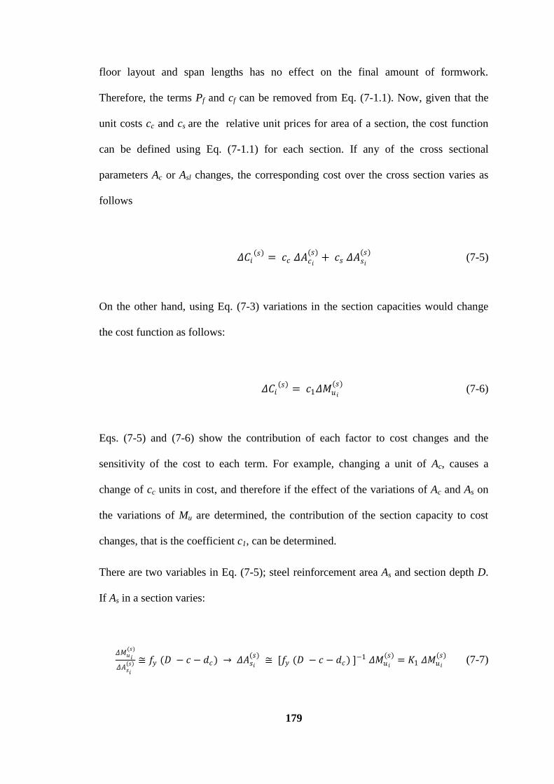
179
floor layout and span lengths has no effect on the final amount of formwork.
Therefore, the terms Pf and cf can be removed from Eq. (7-1.1). Now, given that the
unit costs cc and cs are the relative unit prices for area of a section, the cost function
can be defined using Eq. (7-1.1) for each section. If any of the cross sectional
parameters Ac or Asl changes, the corresponding cost over the cross section varies as
follows
𝛥𝐶𝑖 𝑠 = 𝑐𝑐 𝛥𝐴𝑐𝑖
(𝑠)+ 𝑐𝑠 𝛥𝐴𝑠𝑖
(𝑠) (7-5)
On the other hand, using Eq. (7-3) variations in the section capacities would change
the cost function as follows:
𝛥𝐶𝑖 𝑠 = 𝑐1𝛥𝑀𝑢𝑖
(𝑠) (7-6)
Eqs. (7-5) and (7-6) show the contribution of each factor to cost changes and the
sensitivity of the cost to each term. For example, changing a unit of Ac, causes a
change of cc units in cost, and therefore if the effect of the variations of Ac and As on
the variations of Mu are determined, the contribution of the section capacity to cost
changes, that is the coefficient c1, can be determined.
There are two variables in Eq. (7-5); steel reinforcement area As and section depth D.
If As in a section varies:
𝛥𝑀𝑢𝑖
(𝑠)
𝛥𝐴𝑠𝑖
(𝑠) ≅ 𝑓𝑦 (𝐷 − 𝑐 − 𝑑𝑐) → 𝛥𝐴𝑠𝑖
(𝑠) ≅ [𝑓𝑦 (𝐷 − 𝑐 − 𝑑𝑐) ]−1 𝛥𝑀𝑢 𝑖
(𝑠)= 𝐾1 𝛥𝑀𝑢 𝑖
(𝑠) (7-7)
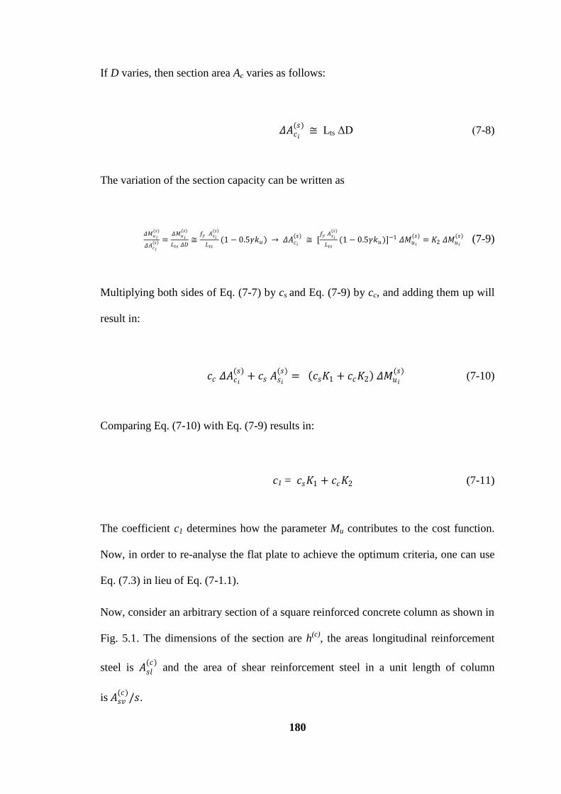
180
If D varies, then section area Ac varies as follows:
𝛥𝐴𝑐𝑖
(𝑠) ≅ Lts ΔD (7-8)
The variation of the section capacity can be written as
𝛥𝑀𝑢 𝑖
(𝑠)
𝛥𝐴𝑐𝑖
(𝑠) =𝛥𝑀𝑢 𝑖
(𝑠)
𝐿𝑡𝑠 𝛥𝐷≅
𝑓𝑦 𝐴𝑠𝑖
(𝑠)
𝐿𝑡𝑠(1 − 0.5𝛾𝑘𝑢) → 𝛥𝐴𝑐𝑖
(𝑠) ≅ [
𝑓𝑦 𝐴𝑠𝑖
(𝑠)
𝐿𝑡𝑠(1 − 0.5𝛾𝑘𝑢)]−1 𝛥𝑀𝑢 𝑖
(𝑠)= 𝐾2 𝛥𝑀𝑢 𝑖
(𝑠) (7-9)
Multiplying both sides of Eq. (7-7) by cs and Eq. (7-9) by cc, and adding them up will
result in:
𝑐𝑐 𝛥𝐴𝑐𝑖
(𝑠)+ 𝑐𝑠 𝐴𝑠𝑖
(𝑠)= 𝑐𝑠𝐾1 + 𝑐𝑐𝐾2 𝛥𝑀𝑢𝑖
(𝑠) (7-10)
Comparing Eq. (7-10) with Eq. (7-9) results in:
c1 = 𝑐𝑠𝐾1 + 𝑐𝑐𝐾2 (7-11)
The coefficient c1 determines how the parameter Mu contributes to the cost function.
Now, in order to re-analyse the flat plate to achieve the optimum criteria, one can use
Eq. (7.3) in lieu of Eq. (7-1.1).
Now, consider an arbitrary section of a square reinforced concrete column as shown in
Fig. 5.1. The dimensions of the section are h(c)
, the areas longitudinal reinforcement
steel is 𝐴𝑠𝑙(𝑐)
and the area of shear reinforcement steel in a unit length of column
is 𝐴𝑠𝑣(𝑐)
/𝑠.

181
Now, consider Eq. (7-12) as a potential alternative cost functions to Eq. (7-1.2) in an
arbitrary RC column section.
𝐶𝑖 𝑐 = 𝑐2𝑁𝑢𝑖
(𝑐)+ 𝑐3 𝑀𝑢𝑖
(𝑐)+ 𝑐4 𝑉𝑢𝑖
(𝑐) (7-12)
where 𝑁𝑢𝑖
(𝑐), 𝑀𝑢𝑖
(𝑐)and 𝑉𝑢𝑖
(𝑐) are the axial load carrying capacity, bending moment
capacities, and the shear capacity of the ith column section respectively. If an
appropriate set of {c2, c3, c4} could be found, in such a way that Eq. (7-13) represents
the cost of the section, the design variables would shift from 𝐴𝑐(𝑐)
, 𝐴𝑠𝑙(𝑐)
, 𝐴𝑠𝑣 𝑐
and
𝑃𝑓 𝑐
to 𝑁𝑢(𝑐)
, 𝑀𝑢(𝑐)
and 𝑉𝑢(𝑐)
.
The capacity or the ultimate strength of the section in axial compression, flexure, and
shear for a column section can be obtained from Eq. (7-13) through Eq. (7-15).
𝑁𝑢 (𝑐)
≅ 0.85𝛾𝑘𝑢 𝑓𝑐′(𝑐)𝑑 𝑐 + 𝐸𝑠 𝐴𝑠𝑙𝑖
(𝑐)휀𝑖
𝑛𝑖 (7-13)
𝑀𝑢 (𝑐)
= 𝑁𝑢 (𝑐)
𝑒 ≅ 0.85𝛾𝑘𝑢 𝑓𝑐′(𝑐)𝑑 𝑐 𝑒𝑐 + 𝐸𝑠 𝐴𝑠𝑙𝑖
(𝑐)휀𝑖𝑒𝑖
𝑛𝑖 (7-14)
𝑉𝑢 (𝑏)
≅𝑓𝑦𝑣 𝑑
(𝑐)𝐴𝑠𝑣 𝑐
𝑠+ 𝛽(𝑐)2
(𝑓𝑐′)0.5 (7-15)
where Es is the modulus of elasticity of reinforcement, 𝐴𝑠𝑙𝑖
(𝑐) and 𝑒𝑖 are respectively the
cross sectional area of reinforcement and the distance from the extreme compression
fibre for each bar, n is the number of bars in a column, and 휀𝑖 is the strain in
reinforcement. The parameters e and 𝑒𝑐 are the eccentricity of the axial force from the
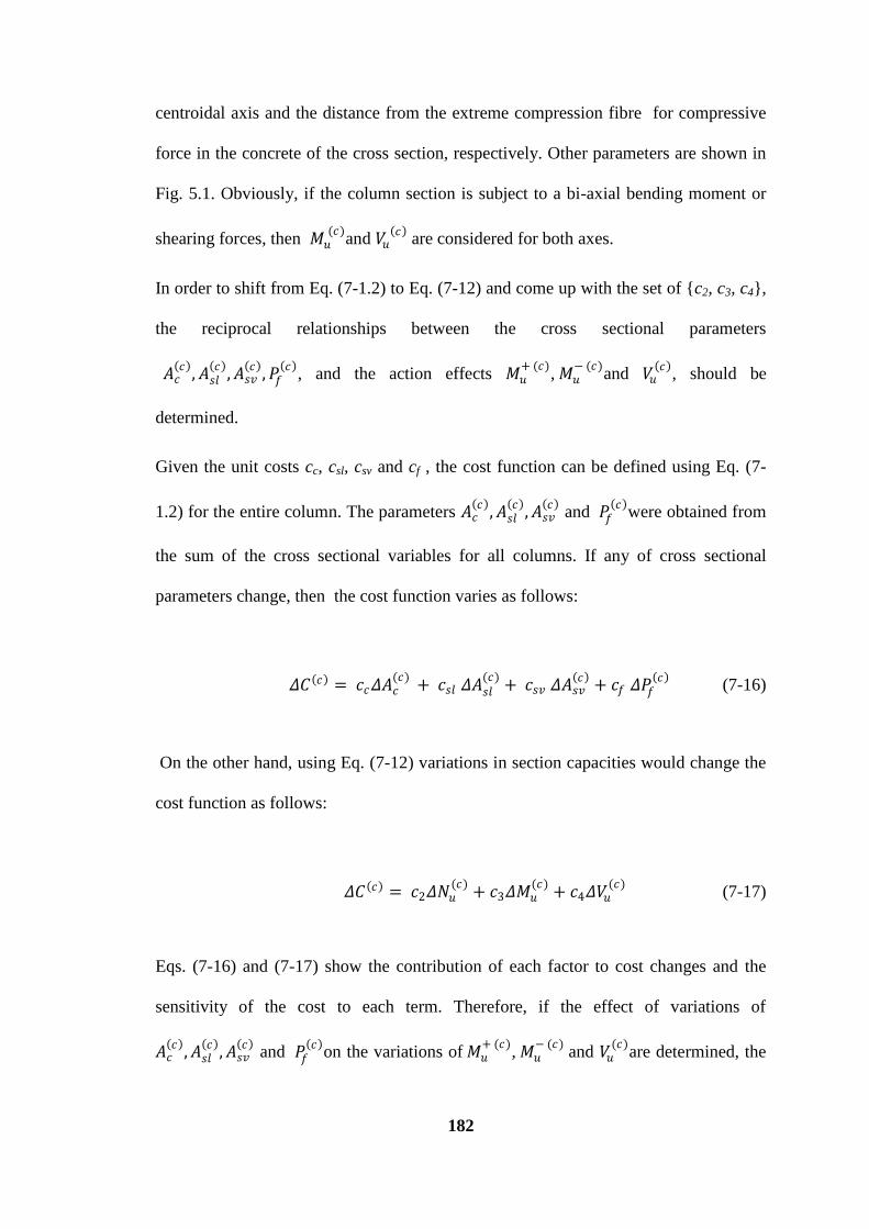
182
centroidal axis and the distance from the extreme compression fibre for compressive
force in the concrete of the cross section, respectively. Other parameters are shown in
Fig. 5.1. Obviously, if the column section is subject to a bi-axial bending moment or
shearing forces, then 𝑀𝑢 (𝑐)
and 𝑉𝑢 𝑐
are considered for both axes.
In order to shift from Eq. (7-1.2) to Eq. (7-12) and come up with the set of {c2, c3, c4},
the reciprocal relationships between the cross sectional parameters
𝐴𝑐 𝑐
, 𝐴𝑠𝑙 𝑐
, 𝐴𝑠𝑣 𝑐
, 𝑃𝑓 𝑐
, and the action effects 𝑀𝑢+ (𝑐)
, 𝑀𝑢− (𝑐)
and 𝑉𝑢 𝑐
, should be
determined.
Given the unit costs cc, csl, csv and cf , the cost function can be defined using Eq. (7-
1.2) for the entire column. The parameters 𝐴𝑐 𝑐
, 𝐴𝑠𝑙 𝑐
, 𝐴𝑠𝑣 𝑐
and 𝑃𝑓 𝑐
were obtained from
the sum of the cross sectional variables for all columns. If any of cross sectional
parameters change, then the cost function varies as follows:
𝛥𝐶 𝑐 = 𝑐𝑐𝛥𝐴𝑐(𝑐)
+ 𝑐𝑠𝑙 𝛥𝐴𝑠𝑙(𝑐)
+ 𝑐𝑠𝑣 𝛥𝐴𝑠𝑣 𝑐
+ 𝑐𝑓 𝛥𝑃𝑓 𝑐
(7-16)
On the other hand, using Eq. (7-12) variations in section capacities would change the
cost function as follows:
𝛥𝐶 𝑐 = 𝑐2𝛥𝑁𝑢(𝑐)
+ 𝑐3𝛥𝑀𝑢(𝑐)
+ 𝑐4𝛥𝑉𝑢(𝑐)
(7-17)
Eqs. (7-16) and (7-17) show the contribution of each factor to cost changes and the
sensitivity of the cost to each term. Therefore, if the effect of variations of
𝐴𝑐 𝑐
, 𝐴𝑠𝑙 𝑐
, 𝐴𝑠𝑣 𝑐
and 𝑃𝑓 𝑐
on the variations of 𝑀𝑢+ (𝑐)
, 𝑀𝑢− (𝑐)
and 𝑉𝑢(𝑐)
are determined, the
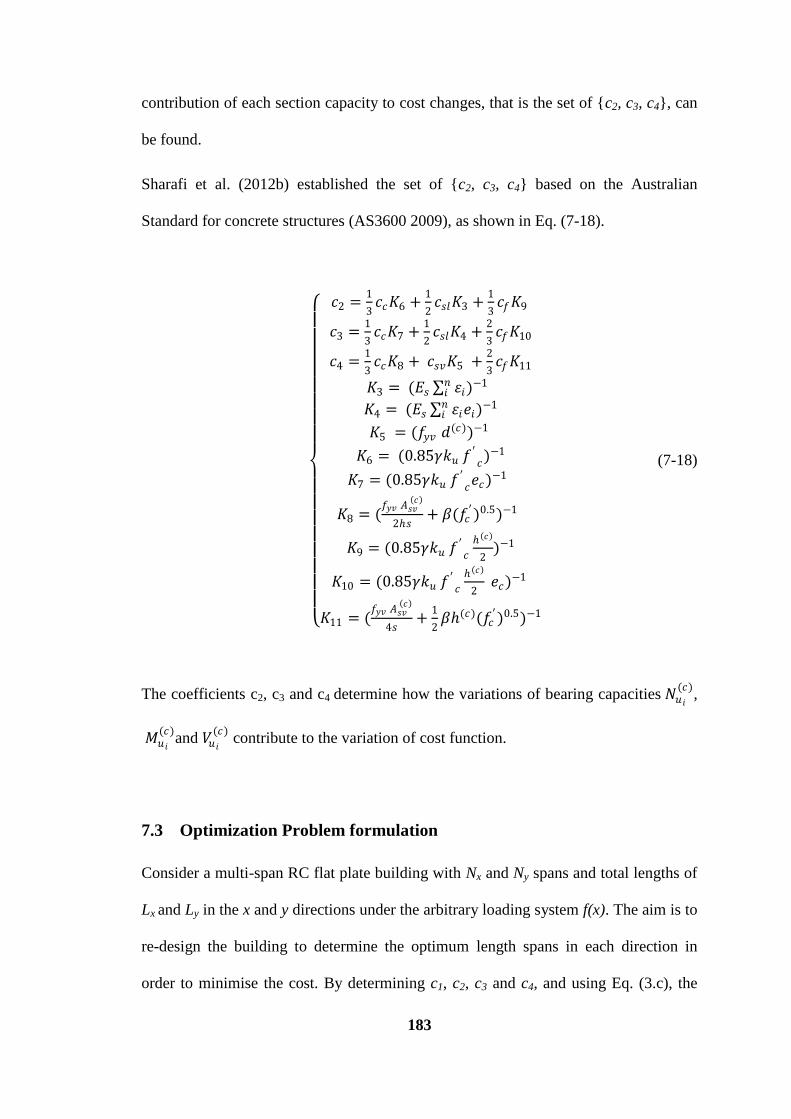
183
contribution of each section capacity to cost changes, that is the set of {c2, c3, c4}, can
be found.
Sharafi et al. (2012b) established the set of {c2, c3, c4} based on the Australian
Standard for concrete structures (AS3600 2009), as shown in Eq. (7-18).
𝑐2 =
1
3𝑐𝑐𝐾6 +
1
2𝑐𝑠𝑙𝐾3 +
1
3𝑐𝑓𝐾9
𝑐3 =1
3𝑐𝑐𝐾7 +
1
2𝑐𝑠𝑙𝐾4 +
2
3𝑐𝑓𝐾10
𝑐4 =1
3𝑐𝑐𝐾8 + 𝑐𝑠𝑣𝐾5 +
2
3𝑐𝑓𝐾11
𝐾3 = (𝐸𝑠 휀𝑖𝑛𝑖 )−1
𝐾4 = (𝐸𝑠 휀𝑖𝑒𝑖𝑛𝑖 )−1
𝐾5 = (𝑓𝑦𝑣 𝑑(𝑐))−1
𝐾6 = (0.85𝛾𝑘𝑢 𝑓′𝑐)−1
𝐾7 = (0.85𝛾𝑘𝑢 𝑓′𝑐𝑒𝑐)−1
𝐾8 = (𝑓𝑦𝑣 𝐴𝑠𝑣
𝑐
2𝑠+ 𝛽(𝑓𝑐
′)0.5)−1
𝐾9 = (0.85𝛾𝑘𝑢 𝑓′𝑐
𝑐
2)−1
𝐾10 = (0.85𝛾𝑘𝑢 𝑓′𝑐
𝑐
2 𝑒𝑐)−1
𝐾11 = (𝑓𝑦𝑣 𝐴𝑠𝑣
𝑐
4𝑠+
1
2𝛽(𝑐)(𝑓𝑐
′)0.5)−1
(7-18)
The coefficients c2, c3 and c4 determine how the variations of bearing capacities 𝑁𝑢𝑖
(𝑐),
𝑀𝑢𝑖
(𝑐)and 𝑉𝑢𝑖
(𝑐) contribute to the variation of cost function.
7.3 Optimization Problem formulation
Consider a multi-span RC flat plate building with Nx and Ny spans and total lengths of
Lx and Ly in the x and y directions under the arbitrary loading system f(x). The aim is to
re-design the building to determine the optimum length spans in each direction in
order to minimise the cost. By determining c1, c2, c3 and c4, and using Eq. (3.c), the
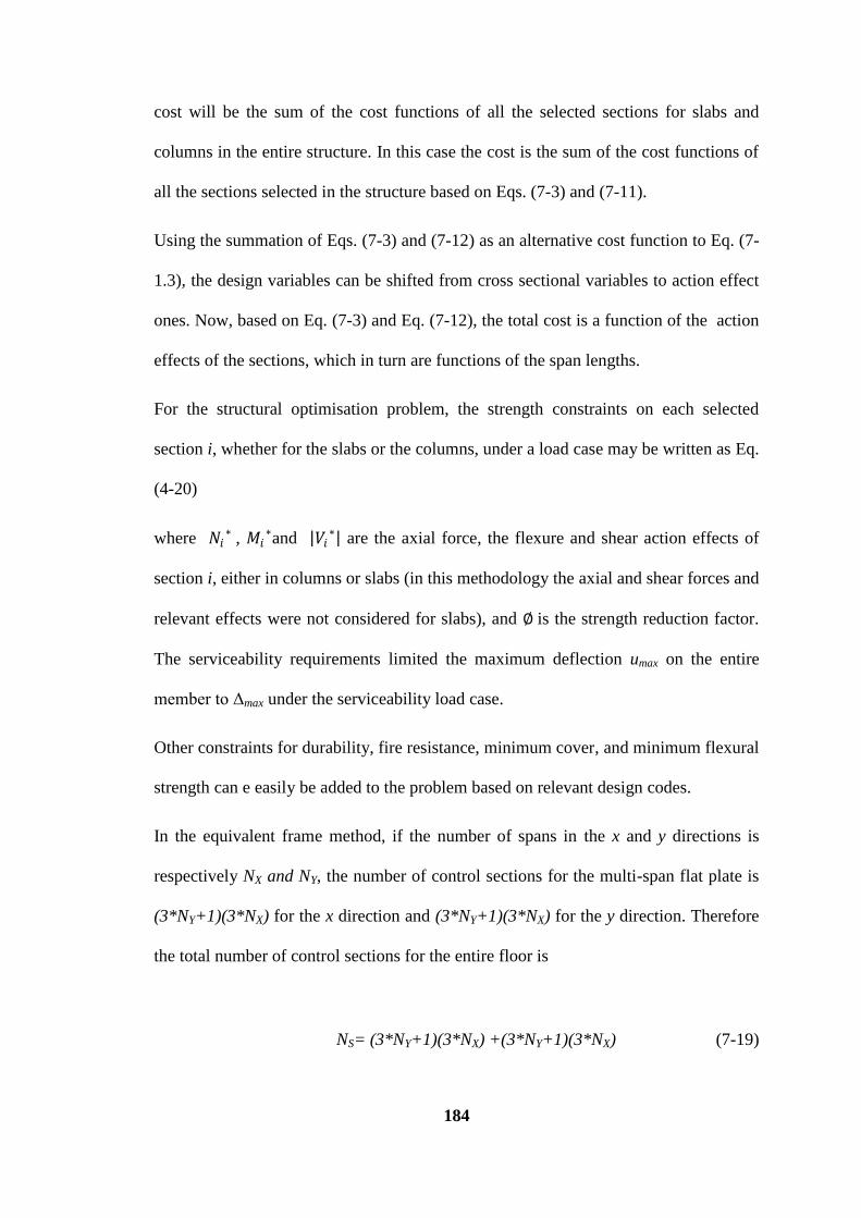
184
cost will be the sum of the cost functions of all the selected sections for slabs and
columns in the entire structure. In this case the cost is the sum of the cost functions of
all the sections selected in the structure based on Eqs. (7-3) and (7-11).
Using the summation of Eqs. (7-3) and (7-12) as an alternative cost function to Eq. (7-
1.3), the design variables can be shifted from cross sectional variables to action effect
ones. Now, based on Eq. (7-3) and Eq. (7-12), the total cost is a function of the action
effects of the sections, which in turn are functions of the span lengths.
For the structural optimisation problem, the strength constraints on each selected
section i, whether for the slabs or the columns, under a load case may be written as Eq.
(4-20)
where 𝑁𝑖∗ , 𝑀𝑖
∗and 𝑉𝑖∗ are the axial force, the flexure and shear action effects of
section i, either in columns or slabs (in this methodology the axial and shear forces and
relevant effects were not considered for slabs), and ∅ is the strength reduction factor.
The serviceability requirements limited the maximum deflection umax on the entire
member to Δmax under the serviceability load case.
Other constraints for durability, fire resistance, minimum cover, and minimum flexural
strength can e easily be added to the problem based on relevant design codes.
In the equivalent frame method, if the number of spans in the x and y directions is
respectively NX and NY, the number of control sections for the multi-span flat plate is
(3*NY+1)(3*NX) for the x direction and (3*NY+1)(3*NX) for the y direction. Therefore
the total number of control sections for the entire floor is
NS= (3*NY+1)(3*NX) +(3*NY+1)(3*NX) (7-19)

185
For columns, one can select as much number of control sections as it takes according
to the desired accuracy. The results obtained from solved numerical instances show
that selecting three or four sections in a typical column is enough to achieve
acceptable results.
Based on AS-3600 (2009), the deflection calculations in slabs can be avoided if the
effective depth is in accordance with the rules for the allowable span/depth ratio. So
based on this rule, the depth constraints on the whole area and all sections of the floor
under a load case may be written as:
𝐿𝑛
𝐷≤ 55[
𝐿𝑛 /𝐿𝑛′
𝑤𝐾𝑝]1/3 (7-20)
where Ln and L'n are the longer and shorter clear spans of the slabs, w is the service
load, including the self weight, and Kp is a coefficient to distinguish between interior
and exterior panels.
For a building with flat plate floor systems under an arbitrary loading system to be
optimally designed for layout, the general formulation for the structural optimisation
problem can be written as follows:
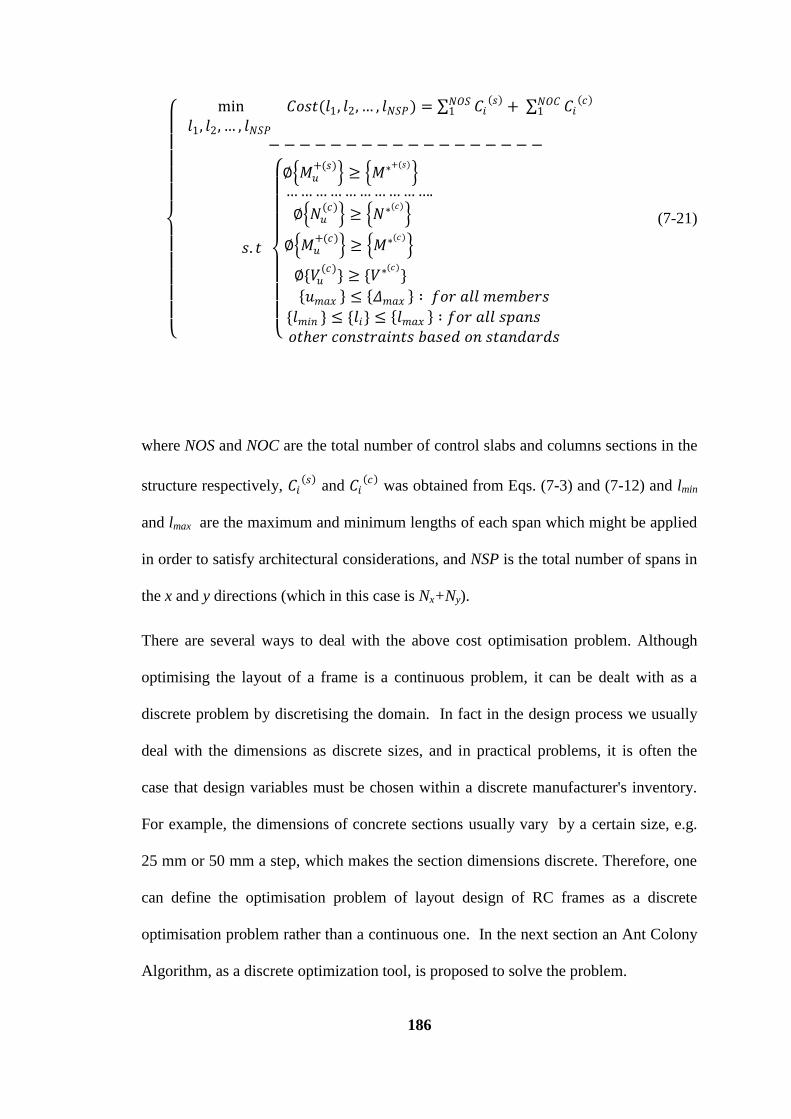
186
min 𝐶𝑜𝑠𝑡(𝑙1, 𝑙2, … , 𝑙𝑁𝑆𝑃) = 𝐶𝑖
𝑠 𝑁𝑂𝑆1 + 𝐶𝑖
𝑐 𝑁𝑂𝐶1
𝑙1, 𝑙2, … , 𝑙𝑁𝑆𝑃 − − − − − − − − − − − − − − − − − −
𝑠. 𝑡
∅ 𝑀𝑢+(𝑠)
≥ 𝑀∗+(𝑠)
… … … … … … …… … ….
∅ 𝑁𝑢(𝑐)
≥ 𝑁∗(𝑐)
∅ 𝑀𝑢+(𝑐)
≥ 𝑀∗(𝑐)
∅{𝑉𝑢(𝑐)
} ≥ {𝑉∗(𝑐)}
𝑢𝑚𝑎𝑥 ≤ 𝛥𝑚𝑎𝑥 ∶ 𝑓𝑜𝑟 𝑎𝑙𝑙 𝑚𝑒𝑚𝑏𝑒𝑟𝑠
{𝑙𝑚𝑖𝑛 } ≤ {𝑙𝑖} ≤ 𝑙𝑚𝑎𝑥 ∶ 𝑓𝑜𝑟 𝑎𝑙𝑙 𝑠𝑝𝑎𝑛𝑠 𝑜𝑡𝑒𝑟 𝑐𝑜𝑛𝑠𝑡𝑟𝑎𝑖𝑛𝑡𝑠 𝑏𝑎𝑠𝑒𝑑 𝑜𝑛 𝑠𝑡𝑎𝑛𝑑𝑎𝑟𝑑𝑠
(7-21)
where NOS and NOC are the total number of control slabs and columns sections in the
structure respectively, 𝐶𝑖 𝑠
and 𝐶𝑖 𝑐
was obtained from Eqs. (7-3) and (7-12) and lmin
and lmax are the maximum and minimum lengths of each span which might be applied
in order to satisfy architectural considerations, and NSP is the total number of spans in
the x and y directions (which in this case is Nx+Ny).
There are several ways to deal with the above cost optimisation problem. Although
optimising the layout of a frame is a continuous problem, it can be dealt with as a
discrete problem by discretising the domain. In fact in the design process we usually
deal with the dimensions as discrete sizes, and in practical problems, it is often the
case that design variables must be chosen within a discrete manufacturer's inventory.
For example, the dimensions of concrete sections usually vary by a certain size, e.g.
25 mm or 50 mm a step, which makes the section dimensions discrete. Therefore, one
can define the optimisation problem of layout design of RC frames as a discrete
optimisation problem rather than a continuous one. In the next section an Ant Colony
Algorithm, as a discrete optimization tool, is proposed to solve the problem.
187
7.4 ACO algorithm
The algorithm attempts to find the optimal lengths of spans using an ACO approach,
to minimise the cost function of a multi-span flat plate building. The basis of the
algorith is similar to the one discussed in Chapter 6. The aim is to find a set of integers
as the lengths of spans in both the x and y directions to minimise the cost function. In
other words the algorithm deals with the discrete form of the problem and the first step
will be discretising the domain. For this purpose, a graph called construction graph
was defined.
To discretise the domain of answers, just as was performed in Chapter 6, assume that
the span lengths are bounded in [Lmin, Lmax] in either direction [Lmin and Lmax might be
different for the x and y direction] with intervals (accuracy) equal to ε, then each Li
rests in the set of {Lmin , Lmin + ε, Lmin + 2ε ,…, Lmax - ε , Lmax}. Obviously, the smaller
ε is chosen, the more accurate results will be obtained and the more running time the
algorithm needs. As shown in Fig. 6.1, an L-shape graph was defined as the
construction graph where the members on the horizontal and vertical wings of the
graph denote spans in the x and y directions respectively. In order for the construction
graph to stand for the multi-span flat plate, the total number of spans and the number
of nodes must be Nx+Ny and (Nx+Ny+1) respectively; hence the construction graph
was defined as a graph with Nx+Ny+1 nodes and ((Lmax -Lmin)/ ε *Nx)+((Lmax - Lmin)/ ε
*Ny) edges. Each pair of nodes are connected with (Lmax - Lmin)/ ε edges, i.e. there are
(Lmax - Lmin)/ ε choices for each Ant on each node to select another one for making its
trail (solution). It should be pointed out that as stated in the definition of constraints,
and shown in Fig. 7-4, Lmax and Lmin might be specified differently for each span, say
Limax and Limin. In this case the number of choices for Ants on each node might differ
188
from the other ones. Now that the construction graph has been prepared the Ants can
start their solution process in three phases (Kaveh and Sharafi 2008b).
1- The phase of initial data processing and preliminary calculation: In this phase the
primary values are given and the calculations start and data are entered. Two groups of
artificial Ants are located on the first and last nodes of both wings of the construction
graph, i.e. Nodes 1 and N+1on the vertical and horizontal wings, to construct their
solution. The lengths of the paths are introduced and the parameters ,, and the
termination criteria are defined, and the initial pheromone and heuristic matrix are
organised. Each value (i,j) of the pheromone matrix and heuristic matrix shows the
tendency of the Ant located on Node i of the construction graph to choose the edge j to
move towards the next node. Since there are as many as (Lmax - Lmin)/ ε edges that
connect every two successive nodes, the dimension of these two matrices will be
(Ny+Nx)*(Lmax - Lmin)/ ε.
To organise the heuristic matrix and initial pheromone matrix (Dorigo and Stützle
2004), we can make use of our experience with structural analysis. Because the
boundary conditions, constraints, and any loads can affect the length of the spans, the
entries of heuristic matrix and initial pheromone matrix might be organised based on
such parameters. Moreover, in order to save time, criteria such as the symmetry of the
plan was considered when the heuristic matrix was defined. In this case the entries of
heuristic matrix relating to preferred choices might receive higher numbers relative to
the entries of the other ones. Using such a heuristic matrix or defining the initial
pheromone matrix using the above mentioned structural rules helps the algorithm
converge sooner. Thus, each value (i,j) of the choice information matrix obtained by
multiplying the corresponding arrays of heuristic matrix by those of the pheromone
189
matrix, shows the tendency or desirability of the Ant located on Node i of the
construction graph to choose Edge j and move towards Node i+1.
2. The phase of constructing the solution: This phase consists of two segments that
form the basis of the heuristic. In the first segment of this phase, using the random
proportional rule of Eq. (3-14), ants located on the starting nodes of the construction
graph, whether Node 1 or Node N+1 on either wing, start to construct their solutions.
That is, two groups of Ants are located on the vertical wing, one at Node 1 and one at
Node Ny+1, and two groups on the horizontal wing do the same at Nodes 1 and Ny+1.
In this method, the feasible neighborhood k
iN is defined as the edges between Nodes i
and i+1, when the Ant is located at Node i in either routs, that is, from Node N+1 to
Node 1 or in reverse on either wing.
The Ant leaves its source Node i{1,2,…,N+1} on the construction graph to its
destination node on the connecting Edges j{1, 2, …, (Lmax - Lmin)/ ε }, using the
random proportional rule, which is similar to the random roulette wheel rule and quite
randomly based on Eq. (3-14). The probability of Edge j being chosen by Ant on Node
i is proportional to the entry (i, j) of the choice information matrix. The bigger the
entry (i,j) the choice matrix is, the more probable Node j is to be chosen by Ant i. The
Ants continue constructing their solution and move from one node to another until
they arrive at Node N+1 on both wings as the end of their trail. The constraint for Ants
on the horizontal wing is that the sum of all spans must be equal to Lx, and Ly for those
on the vertical wing. Therefore, two groups of Ants are located on both ends of both
wings of the graph, so that every edge has the same overall probability of being chosen
by the Ants.
190
After the segment of random choice, the values of Nx+Ny lengths and thereby the new
geometrical layout for the floor was obtained. Through the aforementioned equivalent
frame, the structural analysis method for flat plates, and using the behavioural
constraints, the design actions effects in the identified sections were determined and
by using other constraints the required strength capacities for each section were
calculated. Based on the strength capacity of the sections, the cost function or the cost
of this solution was obtained.
3. The phase of Updating: This phase consists of updating information and statistics,
and then updating the pheromone trails. Using the information obtained in the phase of
constructing the solution, the trail presenting the best cost up to this stage, was
selected as the best iteration so far. Then the pheromone trails of the construction
graph were updated. This is why the Ants were allowed to deposit pheromone on the
edges associated with the best so-far iteration. The process of updating the pheromone
updating consists of two segments. The first segment corresponds to pheromone
evaporation according to Eq. (3-15). In this segment the parameter depends on the
number of steps defined for the termination criteria and the initial pheromone and
heuristic values. The second segment is depositing pheromone according to Eqs. (3-
16) and (3-17). For depositing pheromone, the pheromone values on the edges
associated with the best iteration up to now increased and the Ant deposited an amount
of pheromone equal to 1/cost on the edges of the construction graph associated with
the best iteration so far, and where cost is the value of the cost function obtained from
the best iteration.
The above procedure continues until the termination criterion is satisfied, and then the
optimum spans will be the best solution so far. In each step, a basic structural analysis
is required to calculate the section actions. By making use of a structural analysis

191
approach such as the finite element method, such a calculation takes a small amount of
time for each section. Using Eq. (5.1) as the objective function would be significantly
more time consuming than using Eqs. (7-3) and (7-12). Due to the variation of lengths
in each step, estimating the design variables in each step would be considerably
encumbered, apart from the fact that in each step the algorithm would iteratively need
to deal with the design formulas. Eqs. (7-3) and (7-12) make the optimisation process
much tangible and greatly usable in optimising the cost of large structures.
7.5 Numerical examples
In order to demonstrate the efficiency of the approach proposed for flat plate systems,
two comparative examples were presented. These instances were chosen from a study
on the cost optimisation of flat slabs (Sahab et al. 2005a). The second example was
dealt with in a report on comparative costs of concrete and steel framed buildings
(Goodchild 1993) as well. All the computations were performed on P9700 @2.80 GHz
computer running MATLAB R2009b. In order to ensure that the solution obtained
from ACO was global or near global optimum, many runs were made in parallel. Since
each run is fully independent of the others, the program can be run in parallel so that
the total execution time will be practically the same as that required for a single run.
Example 1: A one storey RC flat plate building with a plan similar to that shown in
Fig. 7-3 with the characteristics of Lx = 20 m, Ly = 18 m, Nx = 4 and Ny = 3 was
considered. The live load and the total dead load were 5.0 and 2.5 kN/m2 respectively.
The average unit price for concrete was assumed to be 55 units/m3, and 3900 units/m
3
for steel. The average unit price for formwork was 20 units/m2. Other design
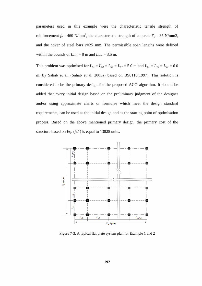
192
parameters used in this example were the characteristic tensile strength of
reinforcement fy = 460 N/mm2, the characteristic strength of concrete f'c = 35 N/mm2,
and the cover of steel bars c=25 mm. The permissible span lengths were defined
within the bounds of Lmax = 8 m and Lmin = 3.5 m.
This problem was optimised for Lx1 = Lx2 = Lx3 = Lx4 = 5.0 m and Ly1 = Ly2 = Ly3 = 6.0
m, by Sahab et al. (Sahab et al. 2005a) based on BS8110(1997). This solution is
considered to be the primary design for the proposed ACO algorithm. It should be
added that every initial design based on the preliminary judgment of the designer
and/or using approximate charts or formulae which meet the design standard
requirements, can be used as the initial design and as the starting point of optimisation
process. Based on the above mentioned primary design, the primary cost of the
structure based on Eq. (5.1) is equal to 13828 units.
Figure 7-3. A typical flat plate system plan for Example 1 and 2
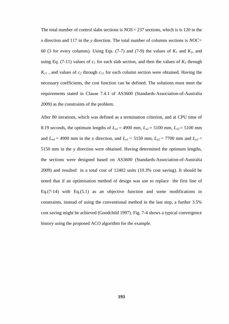
193
The total number of control slabs sections is NOS = 237 sections, which is is 120 in the
x direction and 117 in the y direction. The total number of columns sections is NOC=
60 (3 for every columns). Using Eqs. (7-7) and (7-9) the values of K1 and K2, and
using Eq. (7-11) values of c1 for each slab section, and then the values of K3 through
K11 , and values of c2 through c11 for each column section were obtained. Having the
necessary coefficients, the cost function can be defined. The solutions must meet the
requirements stated in Clause 7.4.1 of AS3600 (Standards-Association-of-Australia
2009) as the constraints of the problem.
After 80 iterations, which was defined as a termination criterion, and at CPU time of
8.19 seconds, the optimum lengths of Lx1 = 4900 mm, Lx2 = 5100 mm, Lx3 = 5100 mm
and Lx4 = 4900 mm in the x direction, and Ly1 = 5150 mm, Ly2 = 7700 mm and Ly3 =
5150 mm in the y direction were obtained. Having determined the optimum lengths,
the sections were designed based on AS3600 (Standards-Association-of-Australia
2009) and resulted in a total cost of 12402 units (10.3% cost saving). It should be
noted that if an optimisation method of design was use to replace the first line of
Eq.(7-14) with Eq.(5.1) as an objective function and some modifications in
constraints, instead of using the conventional method in the last step, a further 3.5%
cost saving might be achieved (Goodchild 1997). Fig. 7-4 shows a typical convergence
history using the proposed ACO algorithm for the example.
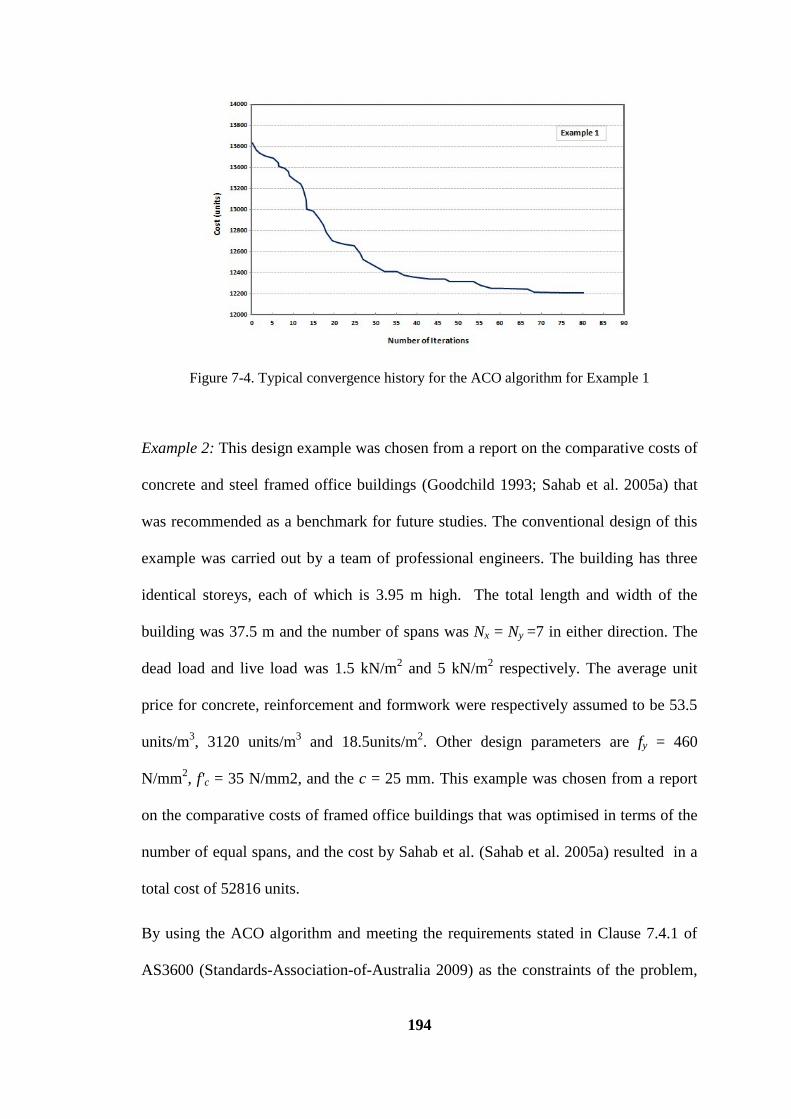
194
Figure 7-4. Typical convergence history for the ACO algorithm for Example 1
Example 2: This design example was chosen from a report on the comparative costs of
concrete and steel framed office buildings (Goodchild 1993; Sahab et al. 2005a) that
was recommended as a benchmark for future studies. The conventional design of this
example was carried out by a team of professional engineers. The building has three
identical storeys, each of which is 3.95 m high. The total length and width of the
building was 37.5 m and the number of spans was Nx = Ny =7 in either direction. The
dead load and live load was 1.5 kN/m2 and 5 kN/m
2 respectively. The average unit
price for concrete, reinforcement and formwork were respectively assumed to be 53.5
units/m3, 3120 units/m
3 and 18.5units/m
2. Other design parameters are fy = 460
N/mm2, f'c = 35 N/mm2, and the c = 25 mm. This example was chosen from a report
on the comparative costs of framed office buildings that was optimised in terms of the
number of equal spans, and the cost by Sahab et al. (Sahab et al. 2005a) resulted in a
total cost of 52816 units.
By using the ACO algorithm and meeting the requirements stated in Clause 7.4.1 of
AS3600 (Standards-Association-of-Australia 2009) as the constraints of the problem,
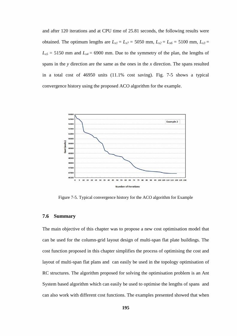
195
and after 120 iterations and at CPU time of 25.81 seconds, the following results were
obtained. The optimum lengths are Lx1 = Lx7 = 5050 mm, Lx2 = Lx6 = 5100 mm, Lx3 =
Lx5 = 5150 mm and Lx4 = 6900 mm. Due to the symmetry of the plan, the lengths of
spans in the y direction are the same as the ones in the x direction. The spans resulted
in a total cost of 46950 units (11.1% cost saving). Fig. 7-5 shows a typical
convergence history using the proposed ACO algorithm for the example.
Figure 7-5. Typical convergence history for the ACO algorithm for Example
7.6 Summary
The main objective of this chapter was to propose a new cost optimisation model that
can be used for the column-grid layout design of multi-span flat plate buildings. The
cost function proposed in this chapter simplifies the process of optimising the cost and
layout of multi-span flat plans and can easily be used in the topology optimisation of
RC structures. The algorithm proposed for solving the optimisation problem is an Ant
System based algorithm which can easily be used to optimise the lengths of spans and
can also work with different cost functions. The examples presented showed that when
196
the proposed algorithm was used the new cost optimisation function provided
satisfactory results.
197
8 Optimum Layout Design for RC Beam-Slab Floor systems
8.1 Introduction
Among the various types of floor systems used in buildings, beam–slab floors (Fig. 8-
1) are quite versatile because they can be used effectively in virtually all types of
buildings. Beam-slab floors are considered to be economical systems for long spans
and high loads (Goodchild et al. 2009). Optimising the layout of the floors is of key
importance for the design and usability of many buildings, because in the preliminary
design of a building with a beam–slab system, determining the length of spans will
affect the location of the columns and consequently, the global layout of the building.
Moreover, concrete floors, including beams and slabs, absorb a large amounts of
money and materials in a building, and therefore optimising the cost of the floors may
have a significant impact on the total cost of the buildings.
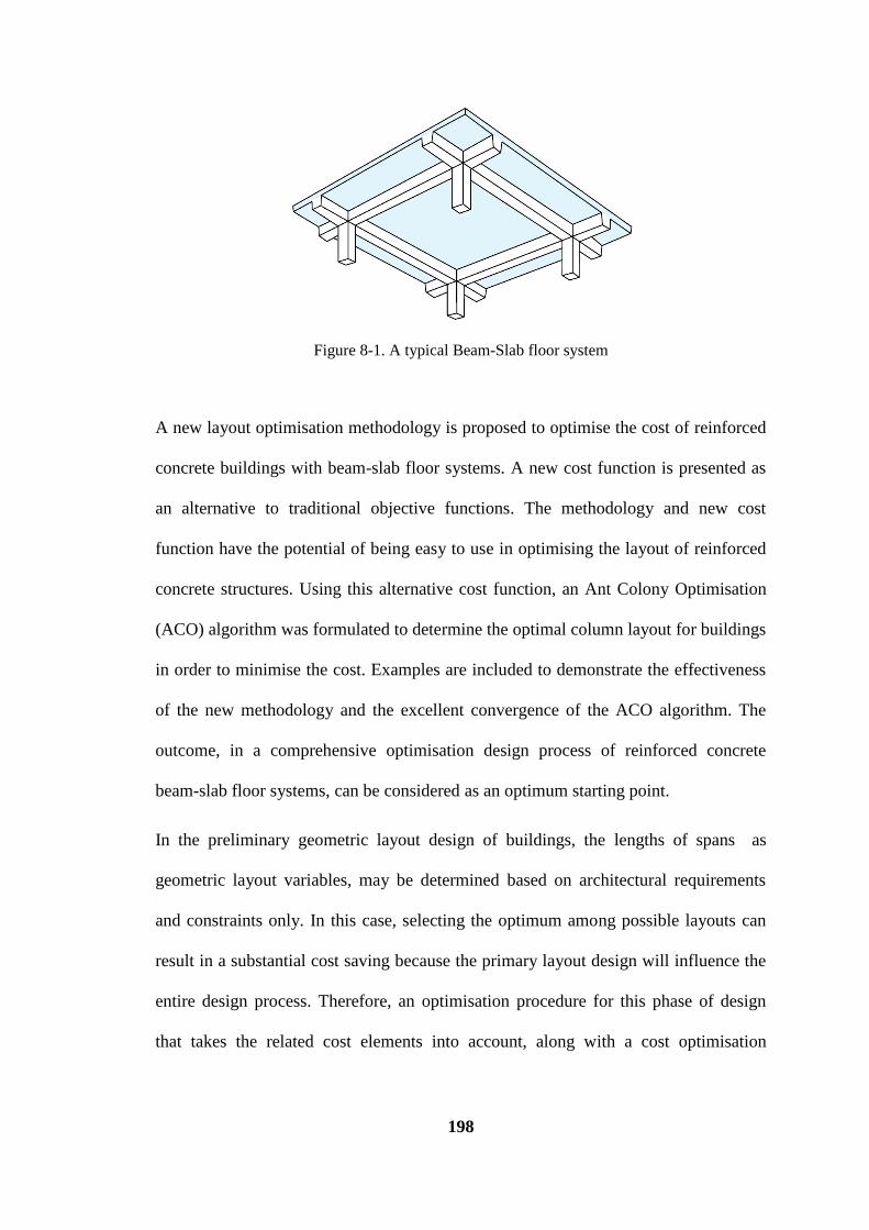
198
Figure 8-1. A typical Beam-Slab floor system
A new layout optimisation methodology is proposed to optimise the cost of reinforced
concrete buildings with beam-slab floor systems. A new cost function is presented as
an alternative to traditional objective functions. The methodology and new cost
function have the potential of being easy to use in optimising the layout of reinforced
concrete structures. Using this alternative cost function, an Ant Colony Optimisation
(ACO) algorithm was formulated to determine the optimal column layout for buildings
in order to minimise the cost. Examples are included to demonstrate the effectiveness
of the new methodology and the excellent convergence of the ACO algorithm. The
outcome, in a comprehensive optimisation design process of reinforced concrete
beam-slab floor systems, can be considered as an optimum starting point.
In the preliminary geometric layout design of buildings, the lengths of spans as
geometric layout variables, may be determined based on architectural requirements
and constraints only. In this case, selecting the optimum among possible layouts can
result in a substantial cost saving because the primary layout design will influence the
entire design process. Therefore, an optimisation procedure for this phase of design
that takes the related cost elements into account, along with a cost optimisation
199
method in the phase of detailed design, can lead to a comprehensive optimal design
procedure.
In concrete structures, at least three different cost items should be considered: the costs
of concrete, steel, and the formwork. In most previous studies the general cost function
for RC slabs is expressed in the following form (Adeli and Sarma 2006)
C =cc Ac + csl Asl + csv Asv + cf Pf (8-1)
where cc, csl, csv and cf are respectively the unit costs for concrete, longitudinal steel,
shear steel, and formwork, and Ac, Asl, Asv and Pf are their corresponding quantities.
Equation (8-1) represents a cost function that only deals with the cross sectional
variables that are mainly appropriate for structures with a small number of members
and a predefined geometric layout. In fact, in the layout design of structures, the cross
sectional variables are functions of the design action effects that are indeterminate and
vary as the layout changes. Therefore, in an iterative procedure for solving an
optimisation problem, each step includes dealing with the structural analysis and the
structural design variables. In such cases, unless alternative design variables are
selected for the cost function, the optimisation procedure might be too unwieldy. Since
cross sectional variables are obtained from implicit functions of structural analysis
outputs based on the relationships and constraints in the design standards which do not
uniquely provide the exact values for these cross sectional parameters, they are not
obtained from an explicit mathematical procedure.
If the reciprocal relationships between the cross sectional design variables and the
design action effects are established, the cost function can be represented by a function
of the design action effects. In the design of a structural member, the design action
200
effects are only determined for the critical sections of the member, and the cross
sectional variables are calculated for each critical section. In other words, knowing the
design action effects in critical sections, all the cross sectional variables and the total
cost as defined by Eq. (8-1) can be calculated.
Using structural analytical outputs such as the internal actions of a member as the
design variables has some advantages over using structural design outcomes such as
the cross sectional variables of a beam. Firstly, the design action effects of each
section can be easily obtained from structural analysis, and in an iterative
mathematical procedure, re-analysing a structure is considerably less time consuming
and more precise than re-designing the structure. Secondly, by using action effects the
cost function will be considered in a section rather than a member because it enables
the designer to select a number of sections for each member and control the cost in the
whole structure, so there is no need to optimise the entire member.
The present work finds the relationships between the variations of action effects of RC
members with the variations of the cross sectional parameters, and determines how
these two types of variables affect each other. A new cost function is then defined such
that it is a function of the action effects rather than the cross sectional parameters. This
formulation was carried out based on the Australian standards for RC structures
(AS3600 2009).
8.2 Mathematical formulation
In the present formulation of optimising the column layout design of RC buildings,
three types of structural members were considered: slabs, columns, and beams.
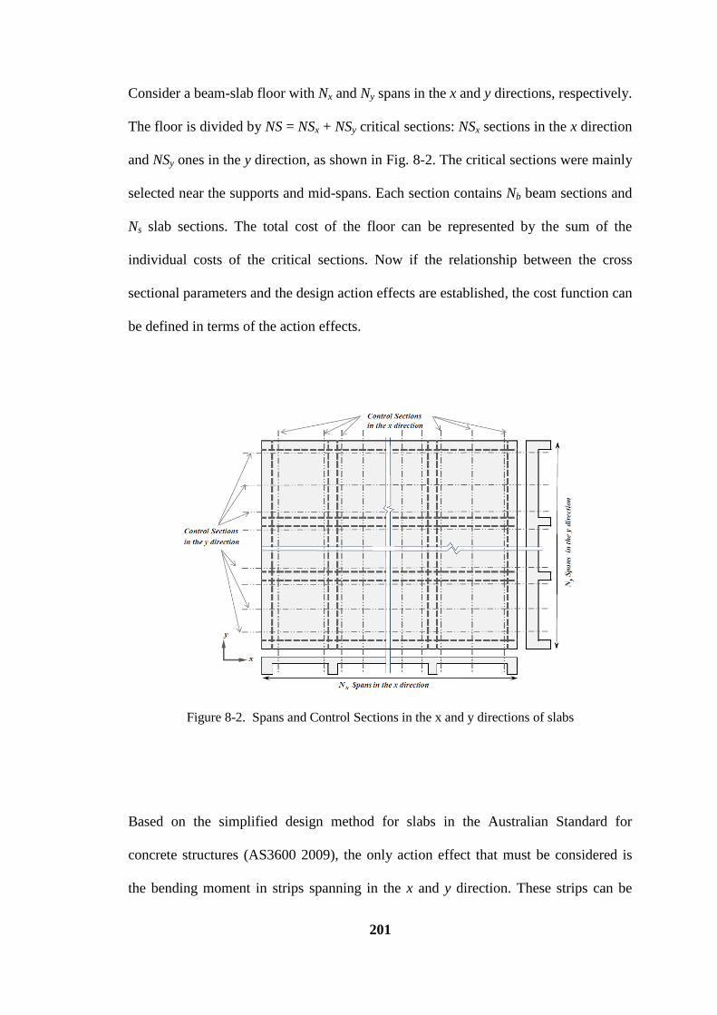
201
Consider a beam-slab floor with Nx and Ny spans in the x and y directions, respectively.
The floor is divided by NS = NSx + NSy critical sections: NSx sections in the x direction
and NSy ones in the y direction, as shown in Fig. 8-2. The critical sections were mainly
selected near the supports and mid-spans. Each section contains Nb beam sections and
Ns slab sections. The total cost of the floor can be represented by the sum of the
individual costs of the critical sections. Now if the relationship between the cross
sectional parameters and the design action effects are established, the cost function can
be defined in terms of the action effects.
Figure 8-2. Spans and Control Sections in the x and y directions of slabs
Based on the simplified design method for slabs in the Australian Standard for
concrete structures (AS3600 2009), the only action effect that must be considered is
the bending moment in strips spanning in the x and y direction. These strips can be
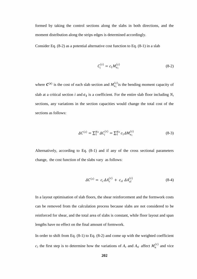
202
formed by taking the control sections along the slabs in both directions, and the
moment distribution along the strips edges is determined accordingly.
Consider Eq. (8-2) as a potential alternative cost function to Eq. (8-1) in a slab
𝐶𝑖(𝑠)
= 𝑐1𝑀𝑢𝑖
𝑠 (8-2)
where 𝑪(𝒔) is the cost of each slab section and 𝑀𝑢𝑖
𝑠 is the bending moment capacity of
slab at a critical section i and 𝒄𝟏 is a coefficient. For the entire slab floor including Ns
sections, any variations in the section capacities would change the total cost of the
sections as follows:
𝛥𝐶 𝑠 = 𝛥𝐶𝑖(𝑠)𝑁𝑠
1 = 𝑐1𝛥𝑀𝑢𝑖
(𝑠)𝑁𝑠1 (8-3)
Alternatively, according to Eq. (8-1) and if any of the cross sectional parameters
change, the cost function of the slabs vary as follows:
𝛥𝐶 𝑠 = 𝑐𝑐𝛥𝐴𝑐(𝑠)
+ 𝑐𝑠𝑙 𝛥𝐴𝑠𝑙(𝑠)
(8-4)
In a layout optimisation of slab floors, the shear reinforcement and the formwork costs
can be removed from the calculation process because slabs are not considered to be
reinforced for shear, and the total area of slabs is constant, while floor layout and span
lengths have no effect on the final amount of formwork.
In order to shift from Eq. (8-1) to Eq. (8-2) and come up with the weighted coefficient
c1 the first step is to determine how the variations of Ac and Asl affect 𝑀𝑢(𝑠)
and vice
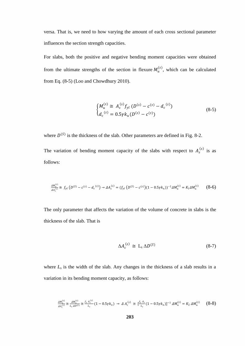
203
versa. That is, we need to how varying the amount of each cross sectional parameter
influences the section strength capacities.
For slabs, both the positive and negative bending moment capacities were obtained
from the ultimate strengths of the section in flexure 𝑀𝑢(𝑠)
, which can be calculated
from Eq. (8-5) (Loo and Chowdhury 2010).
𝑀𝑢
(𝑠)≅ 𝐴𝑠
𝑠 𝑓𝑦𝑙 (𝐷
𝑠 − 𝑐(𝑠) − 𝑑𝑐(𝑠))
𝑑𝑐(𝑠) = 0.5𝛾𝑘𝑢 (𝐷 𝑠 − 𝑐(𝑠))
(8-5)
where 𝐷(𝑆) is the thickness of the slab. Other parameters are defined in Fig. 8-2.
The variation of bending moment capacity of the slabs with respect to 𝐴𝑠 𝑠
is as
follows:
𝛥𝑀𝑢(𝑠)
𝛥𝐴𝑠 𝑠 ≅ 𝑓𝑦𝑙 𝐷
(𝑆) − 𝑐(𝑠) − 𝑑𝑐(𝑠) → 𝛥𝐴𝑠
𝑠 = (𝑓𝑦𝑙 𝐷
(𝑆) − 𝑐(𝑠) (1 − 0.5𝛾𝑘𝑢))−1𝛥𝑀𝑢(𝑠)
= 𝐾1𝛥𝑀𝑢(𝑠) (8-6)
The only parameter that affects the variation of the volume of concrete in slabs is the
thickness of the slab. That is
Δ𝐴𝑐 𝑠
≅ Ls Δ𝐷(𝑆) (8-7)
where Ls is the width of the slab. Any changes in the thickness of a slab results in a
variation in its bending moment capacity, as follows:
𝛥𝑀𝑢(𝑠)
𝛥𝐴𝑐 𝑠 ≅
𝛥𝑀𝑢(𝑠)
𝐿𝑠 𝛥𝐷(𝑆) ≅𝑓𝑦 𝐴𝑠
𝑠
𝐿𝑠(1 − 0.5𝛾𝑘𝑢) → 𝛥 𝐴𝑐
𝑠 ≅ [
𝑓𝑦 𝐴𝑠
𝐿𝑠(1 − 0.5𝛾𝑘𝑢 )]−1 𝛥𝑀𝑢
(𝑠)= 𝐾2 𝛥𝑀𝑢
(𝑠) (8-8)
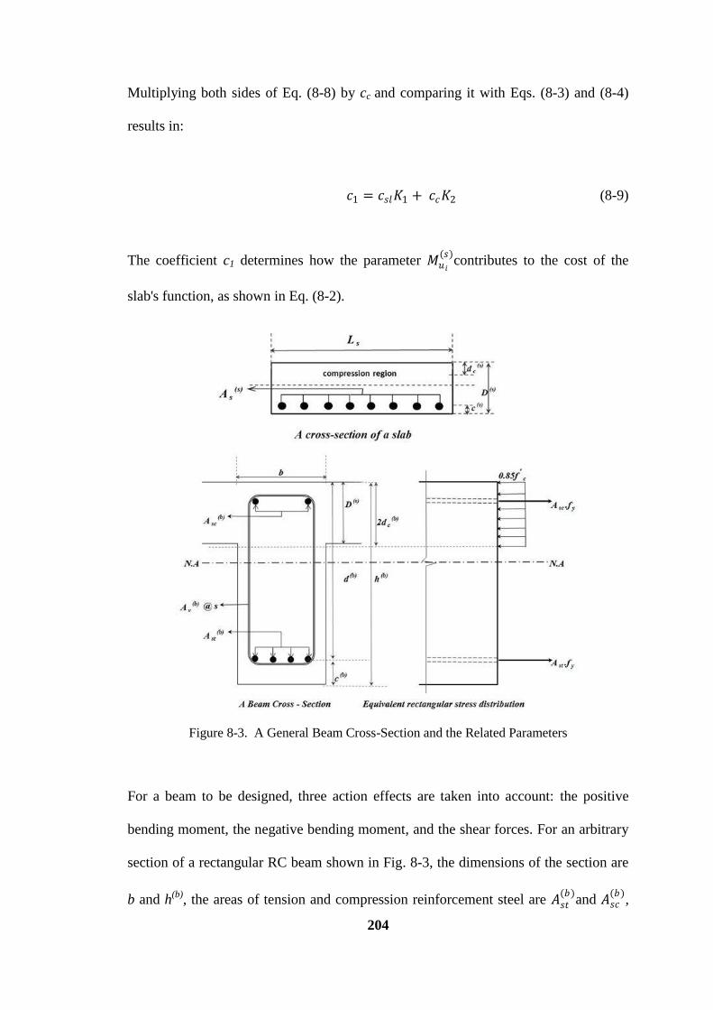
204
Multiplying both sides of Eq. (8-8) by cc and comparing it with Eqs. (8-3) and (8-4)
results in:
𝑐1 = 𝑐𝑠𝑙𝐾1 + 𝑐𝑐𝐾2 (8-9)
The coefficient c1 determines how the parameter 𝑀𝑢𝑖
(𝑠)contributes to the cost of the
slab's function, as shown in Eq. (8-2).
Figure 8-3. A General Beam Cross-Section and the Related Parameters
For a beam to be designed, three action effects are taken into account: the positive
bending moment, the negative bending moment, and the shear forces. For an arbitrary
section of a rectangular RC beam shown in Fig. 8-3, the dimensions of the section are
b and h(b)
, the areas of tension and compression reinforcement steel are 𝐴𝑠𝑡(𝑏)
and 𝐴𝑠𝑐(𝑏)
,
205
and the area of shear reinforcement steel in a unit length of beam is 𝐴𝑠𝑣(𝑏)
/𝑠. The
capacity or the ultimate strength of the section in negative and positive flexure and
shear for Section i are 𝑀𝑢𝑖
− (𝑏) , 𝑀𝑢𝑖
+ (𝑏) and 𝑉𝑢𝑖
(𝑏) respectively.
Consider Eq. (8-10) as a potential alternative cost function to Eq. (8-1) in the ith RC
beam section.
𝐶𝑖 𝑏 = 𝑐2𝑀𝑢𝑖
+ 𝑏 + 𝑐3 𝑀𝑢𝑖
− 𝑏 + 𝑐4 𝑉𝑢𝑖
𝑏 (8-10)
The variations in section capacities would change the cost function as follows:
𝛥𝐶 𝑏 = 𝛥𝐶𝑖 𝑏 𝑁𝑏
1 = (𝑐2 𝛥𝑀𝑢𝑖
+ 𝑏 + 𝑐3 𝛥𝑀𝑢𝑖
− 𝑏 + 𝑐4 𝛥𝑉𝑢𝑖
𝑏 )
𝑁𝑏1 (8-11)
where Nb is the number of control sections in the beams. On the other hand, using Eq.
(8-1), if any of cross sectional parameters change, the cost function varies as follows:
𝛥𝐶 𝑏 = 𝑐𝑐𝛥𝐴𝑐(𝑏)
+ 𝑐𝑠𝑙 𝛥𝐴𝑠𝑙(𝑏)
+ 𝑐𝑠𝑣 𝛥𝐴𝑠𝑣 𝑏
+ 𝑐𝑓 𝛥𝑃𝑓 𝑏
(8-12)
Equations (8-11) and (8-12) show the contribution of each factor to cost changes and
the sensitivity of the cost to each term. For example, changing a unit of 𝐴𝑐 𝑏
causes a
change of cc units in cost. Therefore, if the effects of variations of 𝐴𝑐 𝑏
, 𝐴𝑠𝑙 𝑏
, 𝐴𝑠𝑣 𝑏
and
𝑃𝑓 𝑏
on the variations of 𝑀𝑢+ (𝑏)
, 𝑀𝑢− (𝑏)
and 𝑉𝑢(𝑏)
are established, the contribution of
each section capacity to cost changes, that is the set of {c2, c3, c4} in Eq. (8-10), can be
determined. Sharafi et al. (2012c) established the set of {c2, c3, c4} based on the
Australian Standard for concrete structures (AS3600 2009), as shown in Eq. (8-13)

206
𝑐2 =
1
3𝑐𝑐𝐾6 +
1
2𝑐𝑠𝑙𝐾3 +
2
3𝑐𝑓𝐾9
𝑐3 =1
3𝑐𝑐𝐾5 +
1
2𝑐𝑠𝑙𝐾3 +
2
3𝑐𝑓𝐾8
𝑐4 =1
3𝑐𝑐𝐾7 + 𝑐𝑠𝑣𝐾4 +
2
3𝑐𝑓𝐾10
− − − − − − − − − − − − − − 𝐾3 = (𝑓𝑦𝑙 𝑑
𝑏 (1 − 0.5𝛾𝑘𝑢 ))−1
𝐾4 = 𝑓𝑦𝑣 𝑑 −1
∆𝑉𝑢 𝑏
𝐾5 = 𝑓𝑦𝑙𝐴𝑠𝑐
(𝑏)
𝑏(1 − 0.5𝛾𝑘𝑢)
−1
𝐾6 = 𝑓𝑦𝑙𝐴𝑠𝑡
𝑏
𝑏 1 − 0.5𝛾𝑘𝑢
−1
𝐾7 = 𝑓𝑦𝑙𝐴𝑠𝑡
𝑏
𝑏 1 − 0.5𝛾𝑘𝑢
−1
𝐾8 = 2 𝑓𝑦𝑙 𝐴𝑠𝑐(𝑏)
(1 − 0.5𝛾𝑘𝑢) −1
𝐾9 = 2 𝑓𝑦𝑙 𝐴𝑠𝑡(𝑏)
(1 − 0.5𝛾𝑘𝑢) −1
𝐾10 = [2
𝑓𝑦𝑣 𝐴𝑠𝑣 𝑏
𝑠+ 𝛽𝑏 𝑓 ′
𝑐 12
+1
𝛽𝑑 𝑓 ′𝑐
12
]
(8-13)
where fyl is the yield strength of the longitudinal reinforcement, fyv is the yield strength
of the shear reinforcement, f'c is the characteristic compressive cylinder strength of
concrete at 28 days, 𝑑𝑐(𝑏)
is the distance from the extreme compression fibre of the
concrete to the compressive force. The coefficients 𝛾 and 𝑘𝑢 were calculated based on
the characteristic strength of the concrete and reinforcing steel, β is a coefficient based
on the standard, and s is the centre to centre spacing of shear reinforcement. Other
parameters are defined in Fig. 8-3.
The coefficients c2, c3 and c4 determine how the variations of 𝑀𝑢𝑖
+ (𝑏), 𝑀𝑢𝑖
− (𝑏) and 𝑉𝑢𝑖
(𝑏)
contribute to the variation of cost function for a beam.
For an arbitrary section of a square RC column, as shown in Fig. 8-4, the dimensions
of the section are h(c)
, the area of the longitudinal reinforcement is 𝐴𝑠𝑙(𝑐)
and the area of
shear reinforcement in a unit length of column is 𝐴𝑠𝑣(𝑐)
/𝑠.
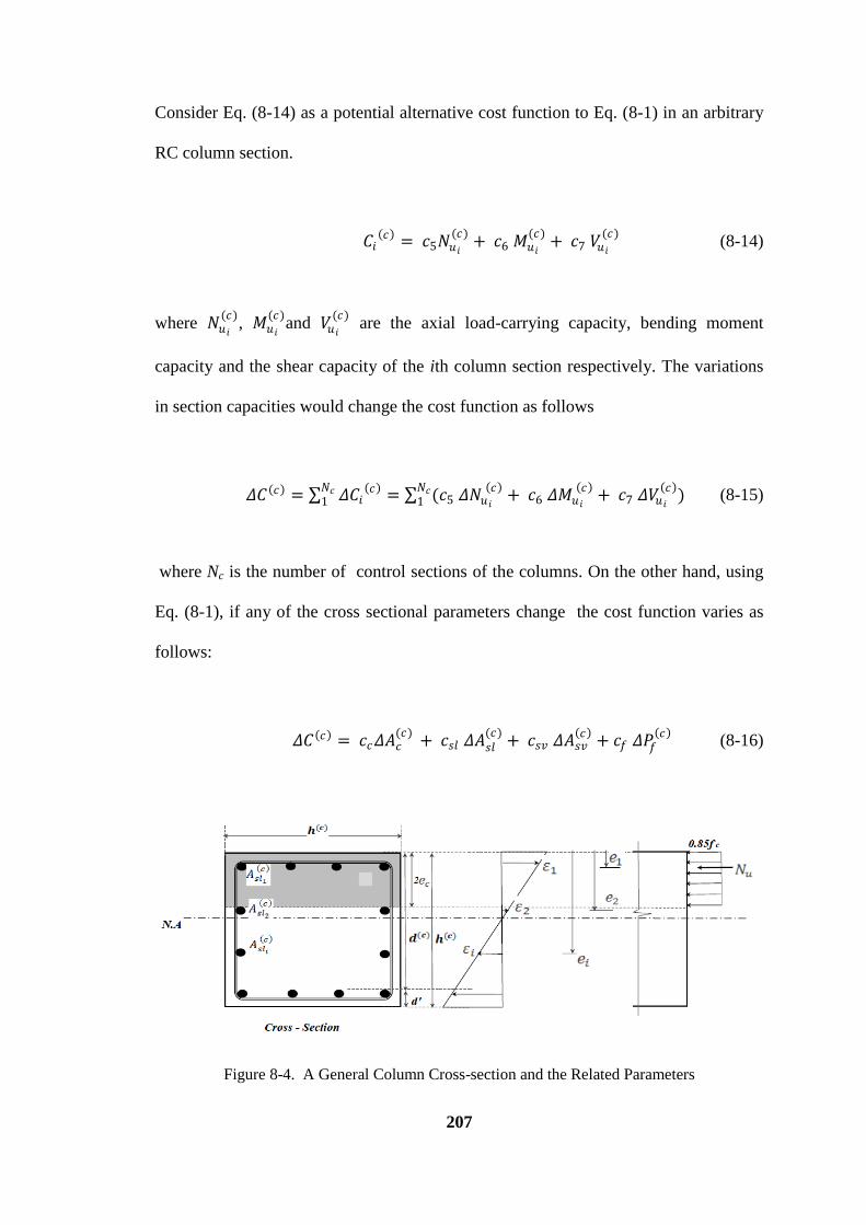
207
Consider Eq. (8-14) as a potential alternative cost function to Eq. (8-1) in an arbitrary
RC column section.
𝐶𝑖 𝑐 = 𝑐5𝑁𝑢𝑖
(𝑐)+ 𝑐6 𝑀𝑢𝑖
(𝑐)+ 𝑐7 𝑉𝑢𝑖
(𝑐) (8-14)
where 𝑁𝑢𝑖
(𝑐), 𝑀𝑢𝑖
(𝑐)and 𝑉𝑢𝑖
(𝑐) are the axial load-carrying capacity, bending moment
capacity and the shear capacity of the ith column section respectively. The variations
in section capacities would change the cost function as follows
𝛥𝐶 𝑐 = 𝛥𝐶𝑖 𝑐 𝑁𝑐
1 = (𝑐5 𝛥𝑁𝑢𝑖
𝑐 + 𝑐6 𝛥𝑀𝑢𝑖
𝑐 + 𝑐7 𝛥𝑉𝑢𝑖
𝑐 )
𝑁𝑐1 (8-15)
where Nc is the number of control sections of the columns. On the other hand, using
Eq. (8-1), if any of the cross sectional parameters change the cost function varies as
follows:
𝛥𝐶 𝑐 = 𝑐𝑐𝛥𝐴𝑐(𝑐)
+ 𝑐𝑠𝑙 𝛥𝐴𝑠𝑙(𝑐)
+ 𝑐𝑠𝑣 𝛥𝐴𝑠𝑣 𝑐
+ 𝑐𝑓 𝛥𝑃𝑓 𝑐
(8-16)
Figure 8-4. A General Column Cross-section and the Related Parameters
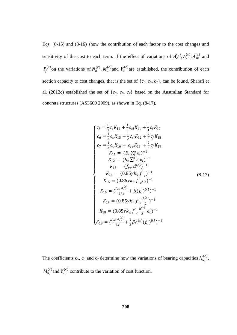
208
Eqs. (8-15) and (8-16) show the contribution of each factor to the cost changes and
sensitivity of the cost to each term. If the effect of variations of 𝐴𝑐 𝑐
, 𝐴𝑠𝑙 𝑐
, 𝐴𝑠𝑣 𝑐
and
𝑃𝑓 𝑐
on the variations of 𝑁𝑢(𝑐)
, 𝑀𝑢(𝑐)
and 𝑉𝑢(𝑐)
are established, the contribution of each
section capacity to cost changes, that is the set of {c5, c6, c7}, can be found. Sharafi et
al. (2012c) established the set of {c5, c6, c7} based on the Australian Standard for
concrete structures (AS3600 2009), as shown in Eq. (8-17).
𝑐5 =
1
3𝑐𝑐𝐾14 +
1
2𝑐𝑠𝑙𝐾11 +
1
3𝑐𝑓𝐾17
𝑐6 =1
3𝑐𝑐𝐾15 +
1
2𝑐𝑠𝑙𝐾12 +
2
3𝑐𝑓𝐾18
𝑐7 =1
3𝑐𝑐𝐾16 + 𝑐𝑠𝑣𝐾13 +
2
3𝑐𝑓𝐾19
𝐾11 = (𝐸𝑠 휀𝑖𝑛𝑖 )−1
𝐾12 = (𝐸𝑠 휀𝑖𝑒𝑖𝑛𝑖 )−1
𝐾13 = (𝑓𝑦𝑣 𝑑(𝑐))−1
𝐾14 = (0.85𝛾𝑘𝑢 𝑓′𝑐)−1
𝐾15 = (0.85𝛾𝑘𝑢 𝑓′𝑐𝑒𝑐)−1
𝐾16 = (𝑓𝑦𝑣 𝐴𝑠𝑣
𝑐
2𝑠+ 𝛽(𝑓𝑐
′)0.5)−1
𝐾17 = (0.85𝛾𝑘𝑢 𝑓′𝑐
𝑐
2)−1
𝐾18 = (0.85𝛾𝑘𝑢 𝑓′𝑐
𝑐
2 𝑒𝑐)−1
𝐾19 = (𝑓𝑦𝑣 𝐴𝑠𝑣
𝑐
4𝑠+
1
2𝛽(𝑐)(𝑓𝑐
′)0.5)−1
(8-17)
The coefficients c5, c6 and c7 determine how the variations of bearing capacities 𝑁𝑢𝑖
(𝑐),
𝑀𝑢𝑖
(𝑐)and 𝑉𝑢𝑖
(𝑐) contribute to the variation of cost function.
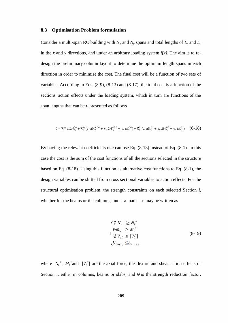
209
8.3 Optimisation Problem formulation
Consider a multi-span RC building with Nx and Ny spans and total lengths of Lx and Ly
in the x and y directions, and under an arbitrary loading system f(x). The aim is to re-
design the preliminary column layout to determine the optimum length spans in each
direction in order to minimise the cost. The final cost will be a function of two sets of
variables. According to Eqs. (8-9), (8-13) and (8-17), the total cost is a function of the
sections' action effects under the loading system, which in turn are functions of the
span lengths that can be represented as follows
𝐶 = 𝑐1𝛥𝑀𝑢𝑖
(𝑠)𝑁𝑠1 + c2 ΔMu i
+ b + c3 ΔMui
− b + c4 ΔVu i
b +
Nb1 (c5 ΔNui
c + c6 ΔMu i
c + c7 ΔVu i
c )
Nc1 (8-18)
By having the relevant coefficients one can use Eq. (8-18) instead of Eq. (8-1). In this
case the cost is the sum of the cost functions of all the sections selected in the structure
based on Eq. (8-18). Using this function as alternative cost functions to Eq. (8-1), the
design variables can be shifted from cross sectional variables to action effects. For the
structural optimisation problem, the strength constraints on each selected Section i,
whether for the beams or the columns, under a load case may be written as
∅ 𝑁𝑢𝑖 ≥ 𝑁𝑖
∗
∅𝑀𝑢𝑖 ≥ 𝑀𝑖
∗
∅ 𝑉𝑢𝑖 ≥ 𝑉𝑖∗
𝑈𝑚𝑎𝑥 𝑖 𝛥𝑚𝑎𝑥 𝑖
(8-19)
where 𝑁𝑖∗ , 𝑀𝑖
∗and 𝑉𝑖∗ are the axial force, the flexure and shear action effects of
Section i, either in columns, beams or slabs, and ∅ is the strength reduction factor,
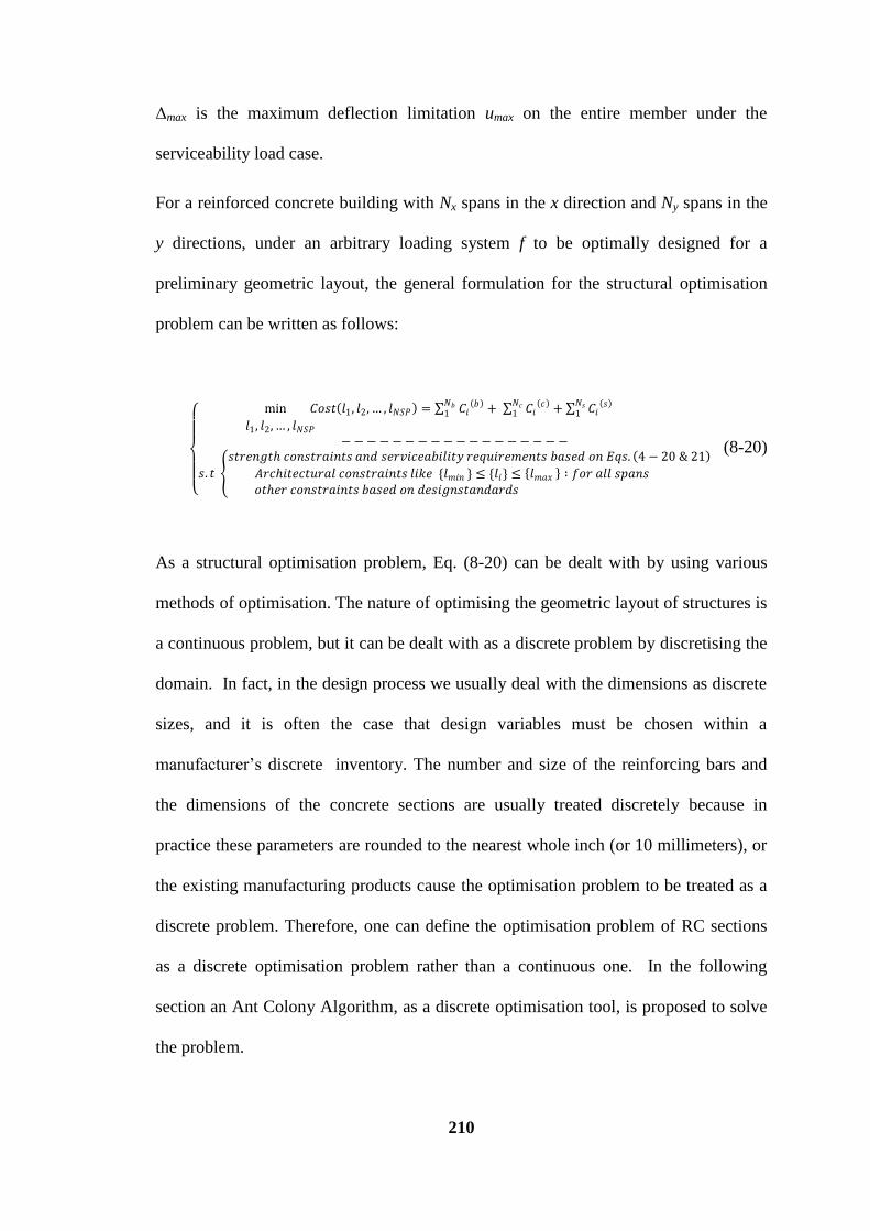
210
Δmax is the maximum deflection limitation umax on the entire member under the
serviceability load case.
For a reinforced concrete building with Nx spans in the x direction and Ny spans in the
y directions, under an arbitrary loading system f to be optimally designed for a
preliminary geometric layout, the general formulation for the structural optimisation
problem can be written as follows:
min 𝐶𝑜𝑠𝑡 𝑙1, 𝑙2, … , 𝑙𝑁𝑆𝑃 = 𝐶𝑖
𝑏 𝑁𝑏1 + 𝐶𝑖
𝑐 𝑁𝑐1 + 𝐶𝑖
𝑠 𝑁𝑠1
𝑙1, 𝑙2, … , 𝑙𝑁𝑆𝑃 − − − − − − − − − − − − − − − − − −
𝑠. 𝑡
𝑠𝑡𝑟𝑒𝑛𝑔𝑡 𝑐𝑜𝑛𝑠𝑡𝑟𝑎𝑖𝑛𝑡𝑠 𝑎𝑛𝑑 𝑠𝑒𝑟𝑣𝑖𝑐𝑒𝑎𝑏𝑖𝑙𝑖𝑡𝑦 𝑟𝑒𝑞𝑢𝑖𝑟𝑒𝑚𝑒𝑛𝑡𝑠 𝑏𝑎𝑠𝑒𝑑 𝑜𝑛 𝐸𝑞𝑠. 4 − 20 & 21
𝐴𝑟𝑐𝑖𝑡𝑒𝑐𝑡𝑢𝑟𝑎𝑙 𝑐𝑜𝑛𝑠𝑡𝑟𝑎𝑖𝑛𝑡𝑠 𝑙𝑖𝑘𝑒 {𝑙𝑚𝑖𝑛 } ≤ {𝑙𝑖} ≤ 𝑙𝑚𝑎𝑥 ∶ 𝑓𝑜𝑟 𝑎𝑙𝑙 𝑠𝑝𝑎𝑛𝑠 𝑜𝑡𝑒𝑟 𝑐𝑜𝑛𝑠𝑡𝑟𝑎𝑖𝑛𝑡𝑠 𝑏𝑎𝑠𝑒𝑑 𝑜𝑛 𝑑𝑒𝑠𝑖𝑔𝑛𝑠𝑡𝑎𝑛𝑑𝑎𝑟𝑑𝑠
(8-20)
As a structural optimisation problem, Eq. (8-20) can be dealt with by using various
methods of optimisation. The nature of optimising the geometric layout of structures is
a continuous problem, but it can be dealt with as a discrete problem by discretising the
domain. In fact, in the design process we usually deal with the dimensions as discrete
sizes, and it is often the case that design variables must be chosen within a
manufacturer‘s discrete inventory. The number and size of the reinforcing bars and
the dimensions of the concrete sections are usually treated discretely because in
practice these parameters are rounded to the nearest whole inch (or 10 millimeters), or
the existing manufacturing products cause the optimisation problem to be treated as a
discrete problem. Therefore, one can define the optimisation problem of RC sections
as a discrete optimisation problem rather than a continuous one. In the following
section an Ant Colony Algorithm, as a discrete optimisation tool, is proposed to solve
the problem.
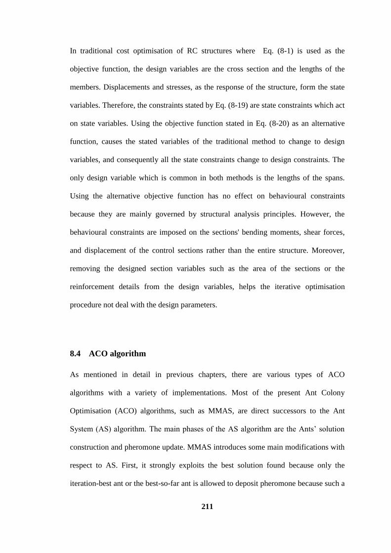
211
In traditional cost optimisation of RC structures where Eq. (8-1) is used as the
objective function, the design variables are the cross section and the lengths of the
members. Displacements and stresses, as the response of the structure, form the state
variables. Therefore, the constraints stated by Eq. (8-19) are state constraints which act
on state variables. Using the objective function stated in Eq. (8-20) as an alternative
function, causes the stated variables of the traditional method to change to design
variables, and consequently all the state constraints change to design constraints. The
only design variable which is common in both methods is the lengths of the spans.
Using the alternative objective function has no effect on behavioural constraints
because they are mainly governed by structural analysis principles. However, the
behavioural constraints are imposed on the sections' bending moments, shear forces,
and displacement of the control sections rather than the entire structure. Moreover,
removing the designed section variables such as the area of the sections or the
reinforcement details from the design variables, helps the iterative optimisation
procedure not deal with the design parameters.
8.4 ACO algorithm
As mentioned in detail in previous chapters, there are various types of ACO
algorithms with a variety of implementations. Most of the present Ant Colony
Optimisation (ACO) algorithms, such as MMAS, are direct successors to the Ant
System (AS) algorithm. The main phases of the AS algorithm are the Ants‘ solution
construction and pheromone update. MMAS introduces some main modifications with
respect to AS. First, it strongly exploits the best solution found because only the
iteration-best ant or the best-so-far ant is allowed to deposit pheromone because such a
212
strategy may result in a stagnation where all the ants follow the same solution due to
the excessive growth of pheromone trails on arcs of a good, although sub-optimal tour.
To counteract this effect, a second modification was introduced by MMAS that limits
the possible range of pheromone trail values to the interval [τmin, τmax]. Moreover, the
pheromone trails were initialised to the upper pheromone trail limit, which, together
with a small pheromone evaporation rate, increased the exploration of solutions at the
start of the search. Finally, in MMAS, the pheromone trails were reinitialised each
time the system approached stagnation or when no improved solution was generated
for a certain number of consecutive iterations.
MMAS achieved a strongly improved performance compared to AS and to other
improved versions of AS, for a wide range of combinatorial optimisation problems.
One feature that MMAS has in common with other improved AS algorithms is that the
best solutions found during the search were strongly exploited to direct the ants‘
search. MMAS related this feature to recent results of the analysis of search space
characteristics for combinatorial optimisation problems. Earlier research has shown
that a strong correlation exists between the quality of the solution and the distance to a
global optimum for the TSP, and for some other problems (Dorigo and Stützle 2004).
MMAS can provide an effective guidance mechanism to direct the search towards the
best solutions, and yet exploiting the best solutions is not the only remedy for
achieving very high performing ACO algorithms. To avoid premature convergence,
the exploitation of the best solutions must be combined with effective mechanisms for
performing a search space exploration. MMAS explicitly addresses this aspect, which
is possibly the main reason why it is currently one of the best performing ACO
algorithms (Stutzle and Hoos 1997).
213
One of the main ideas introduced by MMAS, limited utilisation of the pheromone trail
to prevent premature convergence, can also be applied in a different way, and can be
interpreted as a hybrid between MMAS and action choice rule: while constructing a
solution the ants in action make the best possible choice, as indicated by the
pheromone trail and heuristic information, with a fixed probability p and with a
probability 1−p they make a probabilistic choice shown in Eq. (8-21). With high
parameter values of p and the fact that only the best iteration or the best global
solution was chosen to update the trail, a very strong exploitation of the search history
resulted. When combining the action choice rule with tight pheromone trail limits, a
very promising performance was obtained (Stutzle and Hoos 1997).
The present ACO algorithm for optimising the column layout of RC buildings is an
MMAS algorithm which is described in a flowchart, as shown in Fig. 4-4. The
flowchart comprises three phases: initialising data, constructing an ant solution, and
updating the pheromone. The aim is to determine a set of integers as the span lengths
in boththe x and y directions to minimise the cost function. The algorithm deals with
the discrete form of the problem. The domain must be discretised by forming a
construction graph as a multi-layered graph, as shown in Fig. 4-10, where the number
of layers represents the number of design variables, which are the span lengths in the
x and y directions, and the number of nodes in a particular layer represents the number
of discrete probable values permitted for the corresponding design variable. Thus each
node on the graph is associated with an allowable discrete value of a design variable,
which results in a graph with Nx+Ny layers. Knowing that each span length is bounded
in [𝐿𝑒𝑚𝑎𝑥, 𝐿𝑒𝑚𝑖𝑛
], the permissible values for each span length, which are represented
by the nodes on the graph, can be discretised with intervals (accuracy) equal to ε. That
is, each Le rests in the set of {Lmin , Lmin + ε, Lmin + 2ε ,…, Lmax - ε , Lmax}. Each
214
member of this set corresponds to a node on the graph, so the number of nodes for
each layer is ( 𝐿𝑒𝑚𝑎𝑥− 𝐿𝑒𝑚𝑖𝑛
)/휀. The smaller ε is, the more accurate the results will
be and the more running time the algorithm needs.
In the phase of initial design, some parameters need to be assigned values. The
heuristic values are specified according to the designers' preferences. In the present
case, if there are any preferences for certain span due to say architectural constraints,
higher values are assigned to the heuristic arrays corresponding to those spans. Such
an assignment will cause the desired lengths to be more likely to be chosen by ants for
the corresponding spans. By choosing appropriate values for α and β the degree of
influence of the heuristic values relative to the pheromone trail is set. In order to save
time, some criteria such as the symmetry of the plan were considered when the
heuristic matrix was formed. Using such a heuristic matrix or defining the initial
pheromone matrix using the above mentioned structural rules helped the algorithm
converge sooner.
The initial magnitude of pheromone on the construction graph in MMAS was
initialized to the upper pheromone trail limit, which is a value slightly higher than the
expected amount of pheromone deposited by the ants in one iteration. A rough
estimate of the value can be obtained by setting ∀ 𝑖, 𝑗 𝜏𝑖𝑗 = 𝜏0 = 𝑁𝐴/𝐶𝑛𝑛 where NA is
the number of ants, and Cnn
is the cost of a tour generated by the nearest neighbor
heuristic (Kaveh and Sharafi 2008a; b; 2009). Since boundary conditions, constraints,
and loading condition, can affect the span lengths, while the entries of heuristic matrix
and initial pheromone matrix might be organised to consider such parameters
according to the designer's experience. Each value (i,j) of choice information matrix,
which is obtained by multiplying the corresponding arrays of heuristic matrix by
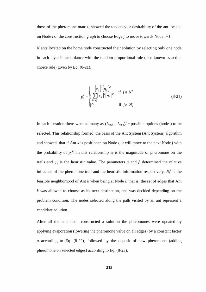
215
those of the pheromone matrix, showed the tendency or desirability of the ant located
on Node i of the construction graph to choose Edge j to move towards Node i+1.
N ants located on the home node constructed their solution by selecting only one node
in each layer in accordance with the random proportional rule (also known as action
choice rule) given by Eq. (8-21).
if 0
if
k
i
k
i
Nl
ilil
ijij
k
ij
Nj
Njp
ki
(8-21)
In each iteration there were as many as (Lmax - Lmin)/ ε possible options (nodes) to be
selected. This relationship formed the basis of the Ant System (Ant System) algorithm
and showed that if Ant k is positioned on Node i, it will move to the next Node j with
the probability of pijk. In this relationship τij is the magnitude of pheromone on the
trails and ηij is the heuristic value. The parameters α and β determined the relative
influence of the pheromone trail and the heuristic information respectively. Nik is the
feasible neighborhood of Ant k when being at Node i, that is, the set of edges that Ant
k was allowed to choose as its next destination, and was decided depending on the
problem condition. The nodes selected along the path visited by an ant represent a
candidate solution.
After all the ants had constructed a solution the pheromones were updated by
applying evaporation (lowering the pheromone value on all edges) by a constant factor
ρ according to Eq. (8-22), followed by the deposit of new pheromone (adding
pheromone on selected edges) according to Eq. (8-23).
216
A(i,j) ρ)τ(1τ ijij (8-22)
A(i,j) , Δτττ best
ijijij (8-23)
where Δτijbest
is 1/Cbest
. The ant which was allowed to add pheromone may be either
the best-so-far, in which case Δτijbest
is 1/Cbs
, or the best iteration, in which case Δτijbest
is 1/Cib
, where Cib
is the length of the best iteration tour.
The pheromone deposit increased the probability that other ants would follow the
same path. That is, by letting ants deposit a higher amount of pheromone on short
paths, the ants‘ path searching was more quickly biased toward the best solutions.
Pheromone evaporation can be seen as an exploration mechanism that avoids quick
convergence of all the ants toward a sub-optimal path. In fact, the decrease in
pheromone intensity favours the exploration of different paths during the whole search
process. Making pheromone update a function of the generated solution quality can
help in directing future ants more strongly towards better solutions.
In general, both the best iteration and the best-so-far update rules are alternatively
used in MMAS. Obviously, the choice of the relative frequency with which the two
pheromone update rules are applied has an influence on how greedy the search is. In
MMAS, the lower and upper limits τmin and τmax on the possible pheromone values on
all edges are imposed in order to avoid a search stagnation. MMAS uses 1/Cbs
to
define τmax: each time a new best-so-far tour is found the value of τmax is updated. The
lower pheromone trail limitis set to τmin= τmax /a where a is a parameter (Stutzle and
Hoos 1997).
217
In each iteration, all the ants in parallel start from the home node and end at the
destination node by randomly selecting a node in each layer. The optimisation process
is terminated if no better solution is found in a pre-specified number of successive
iterations. The above procedure continues until the termination criterion is satisfied,
and then the optimum spans will be given by the best-so-far solution.
MMAS is one of the most studied ACO algorithms and has been extended in many
ways. In one of these extensions the pheromone update rule occasionally uses the best
tour found since the most recent initialisation of the pheromone trails instead of the
best-so-far tour. Experimental results indicate that for small instances it may be best to
use only the best iteration pheromone updates, while for large ones the best
performance is obtained by giving an increasingly stronger emphasis to the best-so-far
tour. This can be achieved by gradually increasing the frequency with which the best-
so-far tour is chosen for the trail update (Stutzle and Hoos 1997).
In each step a basic structural analysis is required to calculate the section action
effects. By making use of a structural analysis approach such as the finite element
method or simplified methods based on the design standards, such a calculation takes a
small amount of time for each section. Using Eq. (8-1) as the objective function would
be significantly more time consuming than using Eq. (8-18). Due to the variation of
lengths in each step the estimation of design variables in each step would be
considerably encumbered, apart from the fact that in each step the algorithm would y
need to iteratively deal with the design formulas. Eq. (8-18) makes the optimisation
process much more tangible and easier to use when optimising the layout of large
structures.
218
8.5 Numerical examples
In order to demonstrate the efficiency of the proposed approach, two comparative
examples are presented. The results obtained from the algorithm were compared with
those in a report on the comparative costs of concrete framed buildings (Goodchild
1997). All the computations were performed on a P9700 @2.80 GHz computer
running MATLAB R2009b. In order to ensure that the solution obtained from ACO
was global or near global optimum, many runs were made in parallel. Since each run
is fully independent of the others, the program can be run in parallel so that the total
execution time will be practically the same as that required for a single run. To prevent
the algorithm from stagnation, in both examples the termination criterion for the ACO
algorithms was defined as the number of iterations when the quality of the solution
after 10 sequential iterations improved by less than 0.02 percent.
Example 1: A four storey RC building with a plan as shown in Fig. 8-6 was optimised.
The live load on intermediate floors was 5.0 kN/m2 and 1.5 kN/m
2 on the roof. The
dead loads are the self-weight and an imposed dead load of 1.5 kN/m2. The average
unit price for concrete was assumed to be 54 units/m3, and 3140 units/m
3 for
reinforcing steel. The average unit price for formwork was 19 units/m2. The
characteristic strength of the main reinforcement fy was 460 N/mm2, the characteristic
strength of the shear reinforcement fyv was 250 N/mm2, the characteristic strength of
concrete f'c was 35 N/mm2, the top and bottom covers of steel bars are 20 and 25 mm
for slabs, respectively, and the cover of bars in columns was 40 mm.
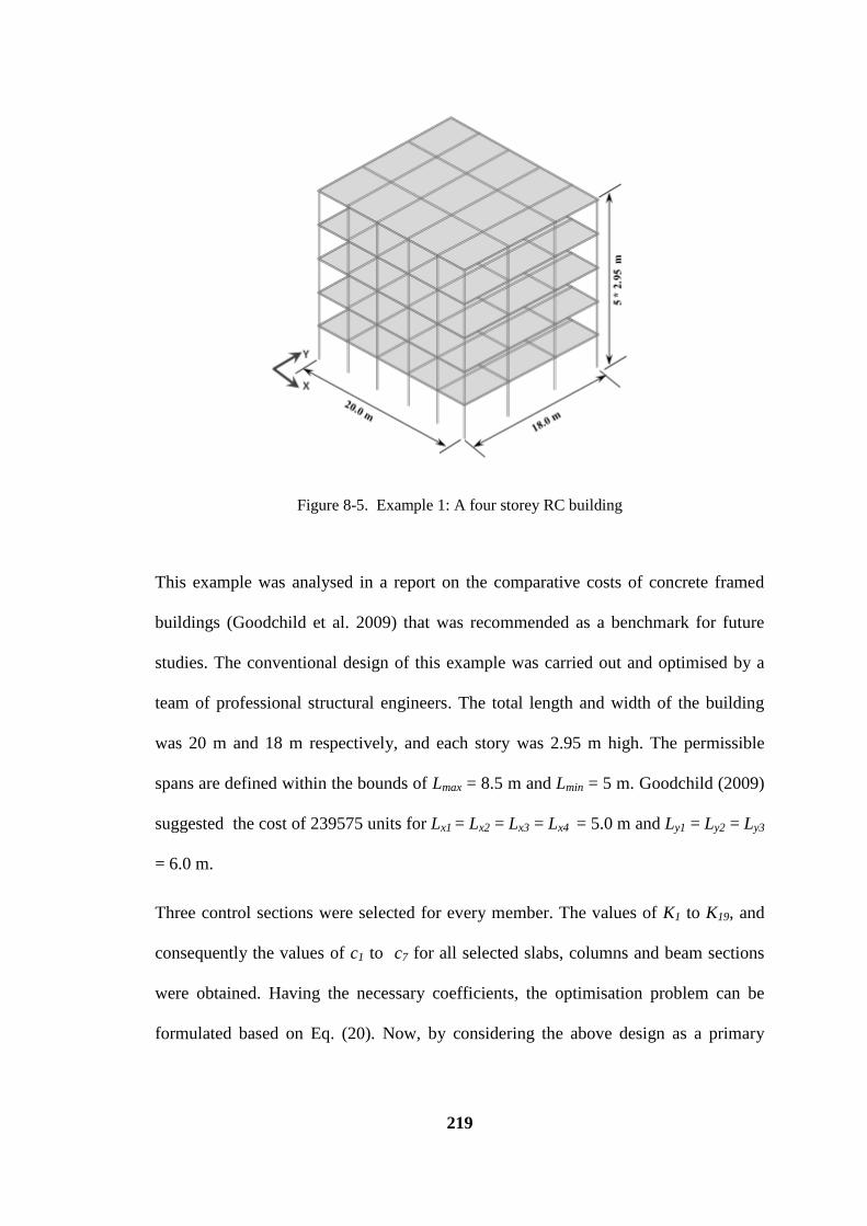
219
Figure 8-5. Example 1: A four storey RC building
This example was analysed in a report on the comparative costs of concrete framed
buildings (Goodchild et al. 2009) that was recommended as a benchmark for future
studies. The conventional design of this example was carried out and optimised by a
team of professional structural engineers. The total length and width of the building
was 20 m and 18 m respectively, and each story was 2.95 m high. The permissible
spans are defined within the bounds of Lmax = 8.5 m and Lmin = 5 m. Goodchild (2009)
suggested the cost of 239575 units for Lx1 = Lx2 = Lx3 = Lx4 = 5.0 m and Ly1 = Ly2 = Ly3
= 6.0 m.
Three control sections were selected for every member. The values of K1 to K19, and
consequently the values of c1 to c7 for all selected slabs, columns and beam sections
were obtained. Having the necessary coefficients, the optimisation problem can be
formulated based on Eq. (20). Now, by considering the above design as a primary
220
design for the proposed ACO algorithm, the Ant algorithm searched for the optimum
spans based on the objective function and by observing other relevant constraints.
Computations were performed on a P9700 @2.80 GHz computer running MATLAB
R2009b.The termination criterion for the ACO algorithms was defined as the number
of iterations when the improvement in the quality of the solution was less than 0.02%
after ten consecutive iterations. After 110 iterations, and at a CPU time of 56.6
seconds, the optimum span lengths of Lx1 = 4550 mm, Lx2 = 5450 mm, Lx3 = 5450 mm
and Lx4 = 4550 mm in the x direction, and Ly1 = 5850 mm, Ly2 = 6300 mm and Ly3 =
5850 mm in the y direction weree obtained, resulting in a total cost of 217534 units,
which equals a 9.2% cost saving compared to the initial design.
Example 2: Consider a multi-span beam-slab floor system with the plan as shown in
Fig. 7-3, with the characteristics of Lx = 20 m, Ly = 25 m, Nx = 4 and Ny = 5 being
considered. The live load and the total dead load were 5.0 and 4.0 kN/m2 respectively.
The floor was supported by beams in two orthogonal directions. The average unit price
for concrete was assumed to be 55 units/m3, and 3900 units/m
3 for steel. The average
unit price for formwork was 20 units/m2. Other design parameters used in this example
are the characteristic tensile strength of reinforcement fy = 460 N/mm2, the
characteristic strength of concrete f'c = 35 N/mm2, and the cover of steel bars c=25
mm. The permissible span lengths were defined within the bounds of Lmax = 8 m and
Lmin = 3.5 m.
This problem was optimally designed for Lx1 = Lx2 = Lx3 = Lx4 = 5.0 m and Ly1 = Ly2 =
Ly3 = Ly4 = Ly5 = 5.0 m, by Goodchild (1993) based on BS8110 (1997). Since the
results for the instances presented comply with the AS 3600 (2009) Standard as well,
221
this solution was considered to be the primary design for the proposed ACO algorithm.
It should be added that every initial design based on the preliminary judgment of the
designer and/or using approximate charts or formulae which meet the requirements of
the design standard can be used as the initial design, and as the starting point for the
optimisation process. Based on the above mentioned primary design, the primary cost
of the structure based on Eq. (8-1) equalled 26751 units.
For this example Ns = 27 control sections were selected for the entire floor, that is, 3
sections for each span. Using Eqs. (8-11) to (8-20) the values of K1 to K10, and using
Eq. (8-22), the values of c1, c2, c3 and c4 were obtained for all sections. By having the
necessary coefficients, the optimisation problem can be formulated based on Eq. (8-
25).
The ACO algorithm attempted to find the optimum spans based on the objective
function and by observing other relevant constraints. In this case no architectural
preferences were considered for the span lengths. In the construction graph phase, the
span lengths are the problem domain and so they were discretised, while for each span
a number of possible lengths were considered. For this purpose the maximum and the
minimum possible span lengths were set as 8.0 and 3.0 metres respectively, and the
problem accuracy (ε) was defined as 0.1 metres to produce the construction graph (see
Fig. 8-6). Ants were then located on the starting and ending nodes to make their trails
in parallel, and then, based on the random proportional rule given by Eq. (8-26) and
the pheromone update given by Eqs. (8-27) to (8-29), the ants found the optimum
length spans. In each iteration the beam needs to be re-analysed according to the new
span lengths to determine the new parameters and the best iteration so far. In the
proposed ACO algorithm for this instance, 10 parallel runs were made to achieve the
optimum solution. The solution continued until the termination criterion was reached.
222
The termination criterion for this problem was defined as the number of iterations
when the improvement in the quality of the solution was less than 0.02% after ten
consecutive iterations.
After 100 iterations as a termination criterion, and at CPU time of 26.76 seconds, the
optimum lengths of Lx1 = 4300 mm, Lx2 = 5400 mm, Lx3 = 5600 mm, Lx4 = 5400 mm
and Lx5 = 4300 mm in the x direction, and Ly1 = 4400 mm, Ly2 = 5600 mm, Ly3 = 5600
mm and Ly4 = 4400 mm in the y direction were obtained. Having determined the
optimum lengths the sections were designed based on AS3600 (2009) resulting in a
total cost of 24823 units (7.2% cost saving).
Example 3: A multi-span beam-slab floor system with the plan shown in Fig. 8-6 was
considered. It had characteristics of Lx = 24 m, Ly = 28.8 m, Nx = 5 and Ny = 6. The live
load, the total dead load, the average unit price for concrete, steel and framework and
other parameters are the same as Example 2. The permissible span lengths were
defined within the bounds of Lmax = 8 m and Lmin = 3.5 m. Goodchild (1993) suggested
a cost of 35139 units for Lx1 = Lx2 = Lx3 = Lx4 = 4.8 m and Ly1 = Ly2 = Ly3 = Ly4 = Ly5 =
4.8 m, on BS8110 (1997). For this example Ns = 33 control sections were selected for
the entire floor, which is 3 sections for each span.
By considering the above design as a primary design for the proposed ACO algorithm,
the ACO algorithm attempted to find the optimum spans based on the objective
function and by observing other relevant constraints. The constraints and architectural
preferences were set the same as Example 2. After 80 iterations, which was defined as
a termination criterion, and at CPU time of 35.22 seconds, the optimum lengths of Lx1
= 4400 mm, Lx2 = 5400 mm, Lx3 = 4400 mm, Lx4 = 5400 mm and Lx5 = 4400 mm in the
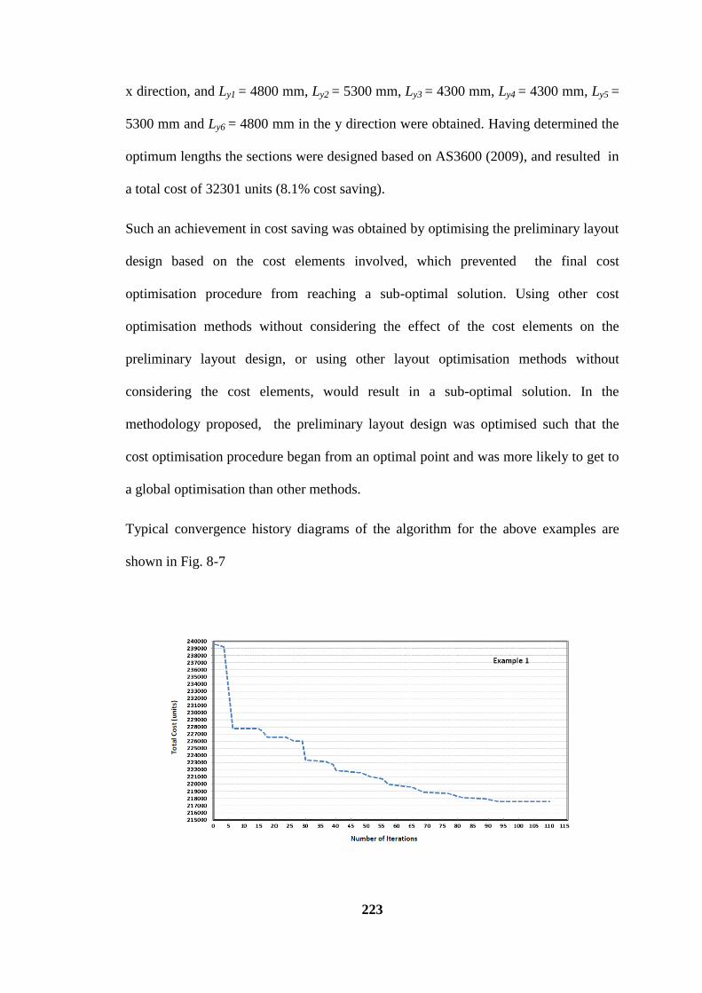
223
x direction, and Ly1 = 4800 mm, Ly2 = 5300 mm, Ly3 = 4300 mm, Ly4 = 4300 mm, Ly5 =
5300 mm and Ly6 = 4800 mm in the y direction were obtained. Having determined the
optimum lengths the sections were designed based on AS3600 (2009), and resulted in
a total cost of 32301 units (8.1% cost saving).
Such an achievement in cost saving was obtained by optimising the preliminary layout
design based on the cost elements involved, which prevented the final cost
optimisation procedure from reaching a sub-optimal solution. Using other cost
optimisation methods without considering the effect of the cost elements on the
preliminary layout design, or using other layout optimisation methods without
considering the cost elements, would result in a sub-optimal solution. In the
methodology proposed, the preliminary layout design was optimised such that the
cost optimisation procedure began from an optimal point and was more likely to get to
a global optimisation than other methods.
Typical convergence history diagrams of the algorithm for the above examples are
shown in Fig. 8-7
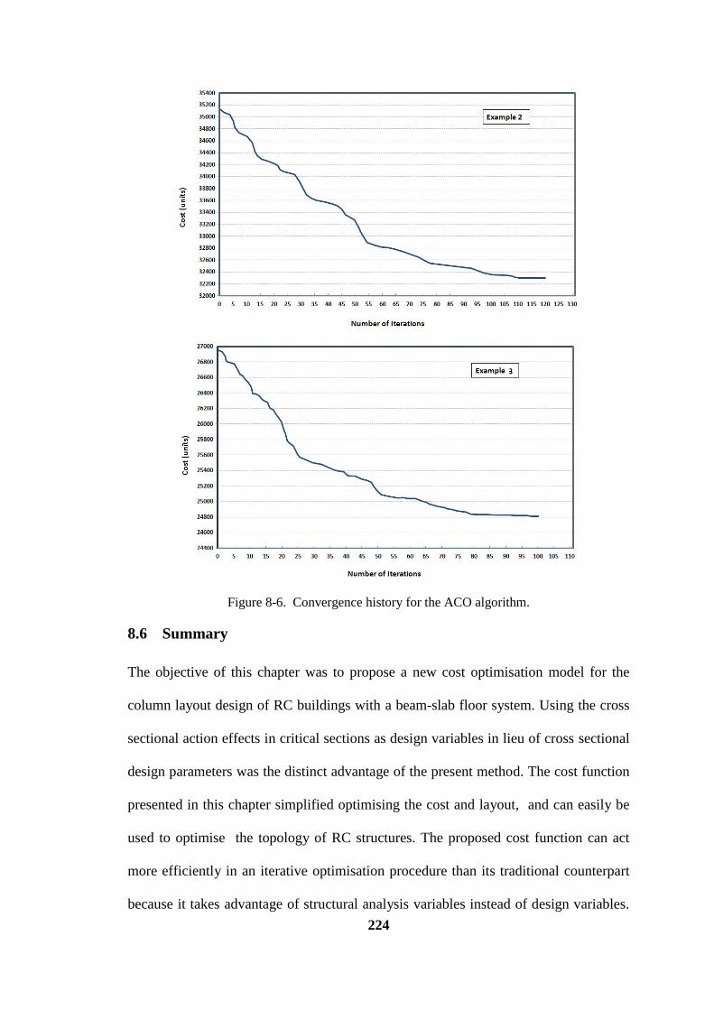
224
Figure 8-6. Convergence history for the ACO algorithm.
8.6 Summary
The objective of this chapter was to propose a new cost optimisation model for the
column layout design of RC buildings with a beam-slab floor system. Using the cross
sectional action effects in critical sections as design variables in lieu of cross sectional
design parameters was the distinct advantage of the present method. The cost function
presented in this chapter simplified optimising the cost and layout, and can easily be
used to optimise the topology of RC structures. The proposed cost function can act
more efficiently in an iterative optimisation procedure than its traditional counterpart
because it takes advantage of structural analysis variables instead of design variables.

225
The proposed algorithm for solving the optimisation problem is an MMAS algorithm
which can easily be used to optimise the span lengths, and is quite capable of working
with different cost functions. The examples presented show that the proposed
algorithm using the new cost optimisation function provided satisfactory results.
226
9 Optimum Layout Design of Rectilinear RC Buildings
9.1 Introduction
In practice, a large number of feasible options are examined during the conceptual
design process; for example, it has been estimated that for a typical commercial
building of 20 stories, if only the architectural and structural aspects are considered
there are approximately 170 million possible design options (Khajehpour and Grierson
2003), but if other aspects of the design are also considered the number of options
would quickly rise to over a billion (Shaw et al. 2008). Therefore, a major barrier to an
automated conceptual optimisation of structures is the large size resulting from the
vast number of design variables and constraints. When it comes to choosing an
appropriate design among a huge number of possible options and dimensions, the
result will be a large combinatorial optimisation problem. Optimisation, on the other
hand can be applied to clearly defined mathematical problems and smooth search
spaces. A typical conceptual design space mainly lacks such features, at least for some
of the objectives because some objectives and constraints are often changed during the

227
design process, which makes an automated preliminary layout optimisation even more
complicated.
In the many optimum design cases, we looked for a set of design variables that were
selected from a given list, and which assure optimum of objective functions together
with a satisfaction of constraints. That is, an optimum design consists of selecting the
best combination of a finite number of structural elements and available parameters.
Such a combinatorial nature, from the mathematical point of view, gives the optimum
design procedure a discrete nature. Progress in modern metaheuristics, along with
rapidly advancing computer technology, enables designers to deal with the problems
of large sizes. Consequently, design systems to help designers with conceptual design
have, over the last decade, been developed using heuristic methods (Soibelman and
Peña-Mora 2000; Sahab et al. 2005a; 2005b; Shaw et al. 2008; Nimtawat and
Nanakorn 2009; 2010).
In this chapter an automated technique is presented for the preliminary layout
optimisation of framed buildings with rectilinear patterns. The method supports all the
buildings of rectilinear (also known as orthogonal or iso-oriented) plans where the
number and size of the spans, plus the shape of the plan can be variables. It means that
this method as a general comprehensive methodology covers all the cases mentioned
in previous chapters. To that end, we took advantage of the knapsack problem as a
basic applied combinatorial optimisation problem.
The objective was to find layouts of maximum profit for frames with a rectilinear
pattern that also satisfy the imposed geometric constraints. The method was presented
in a general form and was not confined to optimisation under a certain type of action
effect and/or geometrical constraints. This gives the methodology the ability of being
228
formulated for various objective functions and constraints, and different structural
systems.
In previous chapters a methodology was proposed to deal with the cost optimisation
problem of preliminary layout design of reinforced concrete frame buildings. We
considered the costs of concrete, longitudinal steel, shear steel and formwork, along
with the other geometric requirements. In the method, the objective function was a
function of the cross sectional action effects, as design variables. Such an objective
function simplifies the optimisation process when the topology optimisation problem
considers the cost elements involved. Some restrictive assumptions were made in the
proposed approach, such as: the building has a rectangular floor plan and the number
of spans in both directions were parallel to the axes of fixed Cartesian coordinates.
In order to solve the optimisation problems arising from the new methodology, the
problems were modelled on the shortest path problems to build a construction graph
that was used for the corresponding ACO algorithms. In fact, so far the shortest path
problem have been used to deal with the optimisation problems arising from the
preliminary layout design of various RC structures, and which have been discussed in
previous chapters. Combinatorial optimisation, arising in various applications in
engineering and management, is one of the most active fields in the interface of
computer science, applied mathematics and engineering. A main motivation for using
combinatorial optimisation methods in engineering and management is that thousands
of real life problems can be formulated as combinatorial optimisation problems.
Furthermore, many of the strongest and most frequently used algorithms in
combinatorial optimisation are historically based on the connection between geometry
and optimisation. This gives such methods the ability of being used to solve
geometrical and topology related optimisation problems due to its ease of formulation
229
(Rosen and Michaels 2000; Lawler 2001; Korte and Vygen 2012). The unified
method presented in this chapter, takes advantages of an applied combinatorial
optimisation problem, namely the knapsack problem.
This chapter presents a combinatorial optimisation approach for the preliminary layout
optimisation of framed reinforced concrete buildings of rectilinear patterns. The new
method, as a general form, supports buildings of orthogonal shapes, including the
rectangular plans. Moreover, the number and size of spans in both directions that are
parallel to the axes of Cartesian coordinates can be variables. The aim of the present
chapter is to propose a unified automated technique for preliminary layout design, by
making use of some basic combinatorial optimisation problems. The objective of this
method is to find layouts of maximum profit for frames of rectilinear shapes that also
satisfy the imposed dimensional, strength, and serviceability constraints. The term
profit, depending on the problem's objective function, can be interpreted as the
minimum cost, minimum lateral displacement, maximum energy saving or any other
objective. The method is presented in a general form and is not confined to
optimisation under a certain type of action effect and/or geometrical constraints.
9.2 Statement of the problem
As mentioned in Chapter 3, there are several problems from the family of knapsack
problems that are considered in this chapter. In all variants of the problem it is
assumed there are some items with a given profit and weight, which are packed in one
or more knapsack of a limited capacity.
In order to describe the column layouts of buildings with an orthogonal floor plan, it is
practical to divide the floor plan into rectangular areas that are represented by four
230
columns on each corner, as shown in Fig. 3-4. Consequently, a column layout can be
described as an arrangement of rectangular areas that completely fill the entire floor
area. In other words, a rectilinear column layout can be created by sub-dividing the
entire floor area into several rectangular areas with no non-rectangular gaps. Assume
that it is desired to design a building with a rectilinear floor plan of required area A, by
filling the floor with rectangular sub-areas. Different arrangements of any set of
rectangular sub-areas that provide the total area of A, and also satisfy the geometric
constraints, are feasible solutions. Each feasible solution represents both a column
layout design and a rectilinear pattern for the floor plan. Therefore, selecting the
optimum set of rectangles and optimum arrangement of them among the sets of
feasible solutions results in an optimum layout design. The objective is a pattern for a
floor plan that includes the columns layout design, and which provides the maximum
profit for the preliminary design phase.
The problem can be stated as follows: As shown in Fig. 3-3, consider a multi-story
framed building that corresponds to the rectilinear floor plan of Fig. 3.2. Any
variation in the building's column layout will lead to a variation in members' cross
sectional design, and consequently a variation in cost (or any other profit that has been
defined as the objective). The question is: what is the optimum rectilinear column
layout pattern which results in the maximum profit? As mentioned before, the profit
can be defined as minimum cost and/or minimum displacements (when designing
buildings for severe lateral loading conditions such as wind or earthquake) or
maximum energy efficiency (when the shape of the building affects the sunny and
shady sides) or any other objective(s) or combination of them.
Using the method explained in Chapter 3, the problem of optimising the layout of
framed building turns to an unbounded multi-constraint multiple knapsack problem.
231
The procedure for modelling the layout optimisation problem on the knapsack
problem can be summarised as follows:
The boundaries of the layout plan are defined by an enclosing rectangle with the
lengths and width of Ly and Lx respectively (Ly ≥ Lx).
Having the maximum and minimum allowable span lengths, the maximum possible
number of spans for each direction is determined. To define a desirable accuracy, a set
of rectangles is formed by discretising the domain for each span. This set contains the
rectangles of all the allowable dimensions that represent the set of items. The sets can
be independently formed for each span due to different limitations on the lengths.
The number of knapsacks m is set to the maximum number of spans in the longest
edge of the enclosing rectangle.
As a bi-constraint problem, two constraints are set for the knapsack‘s capacity. The
first one is the constraint on the weight (length), which is set to the width of the
enclosing rectangle. The second one is the constraint on the number of items, which is
set to the maximum number of spans in the shortest edge of the enclosing rectangle.
The profit can be defined as the inverse of cost and/or the inverse of the lateral
displacement, or any other objectives depending on the problem.
By defining the objective and having a set of items, and a set of knapsacks and their
capacity, optimising the layout of rectilinear frames can be formulated by Eqs. (3-6) to
(3-8).
There are some limitations when selecting a rectangle from the set. In order to have all
the columns on level i in a row and not have any columns off centre, when the first
rectangle (item) is chosen for knapsack i, all the following rectangles must have the
same width. In other words, selecting the first rectangle for each span is equivalent to
232
specifying a length to the span, and all the following rectangles are selected from a
subset of rectangles that are identical in width. Such constraint makes the problem
similar to a multiple-choice knapsack problem. That is, rectangles can be sub-divided
into some classes such that rectangles with an identical length are put in the same
class. Then, exactly one rectangle must be selected from each class for a particular
knapsack.
When defining the knapsacks for each row in the y direction, it should be noted that
each item in each knapsack is corresponding to a rectangle in the plan. In other words
the Item i in Knapsack j corresponds to the Rectangle ij, which is surrounded by
Level i and i+1 in the x direction, and Level j and j+1 in the y direction. Therefore, if a
rectangle with an area rij is selected for the vacant as Item ij (Item i in the Knapsack j),
it consumes one of the total vacant capacities of the knapsack j and a weight of rij from
the total weight capacity aij. If no rectangle is selected for Item ij it means that the sub-
area is void, in which case the void area consumes one of the total vacant capacities of
the Knapsack j and a weight of zero from the total weight capacity.
As explained in Chapter 3, in order to reach practical outcomes such as preventing the
plan from being split into two or more unconnected parts, or in case of preferences,
for some particular shapes, additional constraints can be imposed on the capacity of
each knapsack or the location of voids. In the following some common special cases
are considered.
9.3 Optimisation Problem Formulation
There is not a single layout design solution that has a general optimal performance
with respect to all requirements because the objective criteria are often conflicting, and
233
designers must evaluate different competing criteria to achieve a good compromise
design. That is, the selection of a suitable layout design involves making informed
subjective compromises between conflicting objective criteria.
The objective(s) of the knapsack problem that resulted from the layout optimisation
problem, can be considered as a combination of some architectural, structural, and
environmental objectives such as minimising the disconnected areas, minimising
costs, and lateral movement (for regions at the risk of strong winds or earthquakea),
optimising the sunny or shady areas and surfaces (for environmentally friendly
designs), or any other objectives. Therefore, it is sometimes necessary to deal with a
multi-objective form of the knapsack problem.
A multi-objective optimisation problem f = (f1,f2,…,fQ) is a problem of finding a vector
of decision variables that satisfies the constraints and optimises the vector function f
whose elements f1 to fQ represent the Q number of objective functions, and which
usually conflict with each other. For example, in the knapsack problem, as a result of
layout optimisation, the profit f can be defined as a vector of inverse of cost and
inverse of lateral movement. For the layout optimisation problem the capacity of
knapsack(s) is not related to the number of objectives. Therefore, Eqs. (3-6), (3-7), (3-
8), (3-10) and (3-12) remain unchanged for multi-objective optimisation problems.
The objective functions for multi-objective multiple knapsack problems can be
formulated as follows:
𝑚𝑎𝑥 𝑓 = ( 𝑏𝑖𝑗1 𝑦𝑖𝑗 ,
𝑛
𝑖=1
𝑚
𝑗 =1
𝑏𝑖𝑗2 𝑦𝑖𝑗 , … , 𝑏𝑖𝑗
𝑄𝑦𝑖𝑗
𝑛
𝑖=1
)
𝑚
𝑗 =1
𝑛
𝑖=1
𝑚
𝑗 =1
(9-1)

234
where 𝑏𝑖𝑗𝑞
is the profit of Item i when selected for Knapsack j with respect to the
Objective q.
Now, the problem of optimising the layout of buildings with a rectilinear pattern is a
multi-objective multiple knapsack problem. There are some meta-heuristics such as
evolutionary algorithms for multiple knapsack problems (Kellerer et al. 2004; Soylu
and Köksalan 2009). In a companion paper (Sharafi et al. 2013b), an ant colony
algorithm was used to solve the multi-objective multiple knapsack problem for
optimising the layout of buildings with rectilinear floors, while their application for
reinforced concrete structures was discussed previously.
9.3.1 Formulation for Cost
Consider a multi-storey framed building with a rectilinear floor plan as shown in Fig.
14-1. The RC building is formed of a set of beams, columns, and slabs, and all the
stories have the same floor plan. Any variation in the plan layout will lead to a
variation in the cross sectional design of the members and a consequent variation in
cost and regularity, which is defined as the profit. The question is: what is the
optimum rectilinear layout pattern which results in the maximum profit?
If cc, csl, csv and cf are the unit costs of concrete, longitudinal steel, shear steel and
formwork respectively, and the capacity or the ultimate strength of each section in
negative and positive flexure and shear for section i are 𝑀𝑢𝑖
− (𝑏) , 𝑀𝑢𝑖
+ (𝑏) and 𝑉𝑢𝑖
(𝑏)
respectively, the variation of cost for ith beams section 𝛥𝐶 𝑏 can be presented by Eq.
(9-2) (Sharafi et al. 2012c).
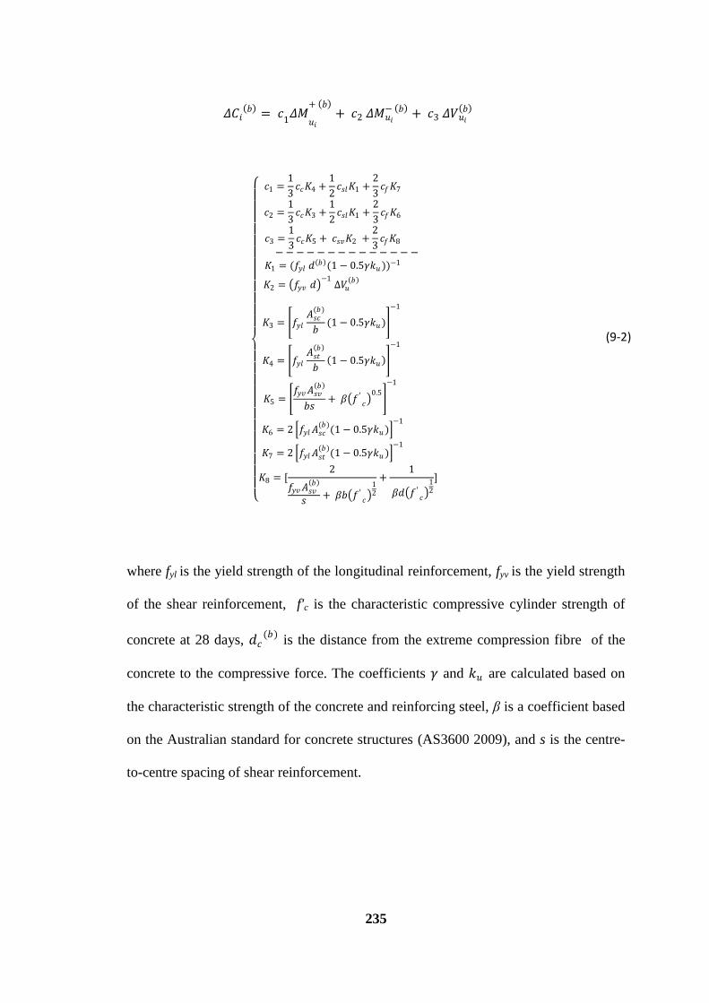
235
𝛥𝐶𝑖 𝑏 = 𝑐
1𝛥𝑀
𝑢𝑖
+ 𝑏 + 𝑐2 𝛥𝑀𝑢𝑖
− 𝑏 + 𝑐3 𝛥𝑉𝑢𝑖
𝑏
𝑐1 =
1
3𝑐𝑐𝐾4 +
1
2𝑐𝑠𝑙𝐾1 +
2
3𝑐𝑓𝐾7
𝑐2 =1
3𝑐𝑐𝐾3 +
1
2𝑐𝑠𝑙𝐾1 +
2
3𝑐𝑓𝐾6
𝑐3 =1
3𝑐𝑐𝐾5 + 𝑐𝑠𝑣𝐾2 +
2
3𝑐𝑓𝐾8
− − − − − − − − − − − − − − 𝐾1 = (𝑓𝑦𝑙 𝑑
𝑏 (1 − 0.5𝛾𝑘𝑢 ))−1
𝐾2 = 𝑓𝑦𝑣 𝑑 −1
∆𝑉𝑢 𝑏
𝐾3 = 𝑓𝑦𝑙
𝐴𝑠𝑐(𝑏)
𝑏(1 − 0.5𝛾𝑘𝑢)
−1
𝐾4 = 𝑓𝑦𝑙
𝐴𝑠𝑡 𝑏
𝑏 1 − 0.5𝛾𝑘𝑢
−1
𝐾5 = 𝑓𝑦𝑣 𝐴𝑠𝑣
𝑏
𝑏𝑠+ 𝛽 𝑓′
𝑐
0.5
−1
𝐾6 = 2 𝑓𝑦𝑙 𝐴𝑠𝑐(𝑏)
(1 − 0.5𝛾𝑘𝑢 ) −1
𝐾7 = 2 𝑓𝑦𝑙 𝐴𝑠𝑡(𝑏)
(1 − 0.5𝛾𝑘𝑢 ) −1
𝐾8 = [2
𝑓𝑦𝑣 𝐴𝑠𝑣 𝑏
𝑠+ 𝛽𝑏 𝑓′
𝑐
12
+1
𝛽𝑑 𝑓′𝑐
12
]
(9-2)
where fyl is the yield strength of the longitudinal reinforcement, fyv is the yield strength
of the shear reinforcement, f'c is the characteristic compressive cylinder strength of
concrete at 28 days, 𝑑𝑐(𝑏)
is the distance from the extreme compression fibre of the
concrete to the compressive force. The coefficients 𝛾 and 𝑘𝑢 are calculated based on
the characteristic strength of the concrete and reinforcing steel, β is a coefficient based
on the Australian standard for concrete structures (AS3600 2009), and s is the centre-
to-centre spacing of shear reinforcement.
236
Figure 9-1. A multi-storey building with a rectilinear frame
For the columns, if 𝑁𝑢𝑖
(𝑐), 𝑀𝑢𝑖
(𝑐)and 𝑉𝑢𝑖
(𝑐) are the axial load-carrying capacity, bending
moment capacity, and the shear capacity of the ith column section respectively, the
variation of cost for the columns section 𝛥𝐶 𝑐 can be presented by Eq. (9-3) (Sharafi
et al. 2012c).
𝛥𝐶𝑖 𝑐 = 𝑐4𝛥𝑁𝑢
(𝑐)+ 𝑐5𝛥𝑀𝑢
(𝑐)+ 𝑐6𝛥𝑉𝑢
(𝑐)
237
𝑐4 =
1
3𝑐𝑐𝐾12
+1
2𝑐𝑠𝑙𝐾9
+1
3𝑐𝑓𝐾15
𝑐5 =1
3𝑐𝑐𝐾13
+1
2𝑐𝑠𝑙𝐾10
+2
3𝑐𝑓𝐾16
𝑐6 =1
3𝑐𝑐𝐾14
+ 𝑐𝑠𝑣𝐾11 +
2
3𝑐𝑓𝐾17
− − − − − − − − − − − − − −
𝐾9 = (𝐸𝑠 휀𝑖
𝑛
𝑖
)
−1
𝐾10 = (𝐸𝑠 휀𝑖𝑒𝑖
𝑛
𝑖
)
−1
𝐾11 = (𝑓𝑦𝑣
𝑑(𝑐))−1
𝐾12 = (0.85𝛾𝑘𝑢 𝑓′𝑐)−1
𝐾13 = (0.85𝛾𝑘𝑢 𝑓′𝑐𝑒𝑐)
−1
𝐾14 = (𝑓
𝑦𝑣 𝐴
𝑠𝑣
𝑐
2𝑠+ 𝛽(𝑓
𝑐′ )
0.5)
−1
𝐾15 = (0.85𝛾𝑘𝑢 𝑓′𝑐
𝑐
2)
−1
𝐾16 = (0.85𝛾𝑘𝑢 𝑓′𝑐
𝑐
2 𝑒𝑐)
−1
𝐾17 = (𝑓
𝑦𝑣 𝐴
𝑠𝑣
𝑐
4𝑠+
1
2𝛽 𝑐 (𝑓
𝑐′ )
0.5)
−1
(9-3)
where Es is the the modulus of elasticity of reinforcement, 𝐴𝑠𝑙𝑖
(𝑐) and 𝑒𝑖 are respectively
the cross sectional area of reinforcement and the distance from the extreme
compression fibre for each bar, n is the number of bars in a column, 휀𝑖 is the strain in
reinforcement. The parameters e and 𝑒𝑐 are the eccentricity of the axial force from the
centroidal axis and the distance from the extreme compression fibre for compressive
force in the concrete of the cross section, respectively.
Also the formulation for Slabs was done in the same way. If 𝑀𝑢𝑖
𝑠 is the bending
moment capacity of the slab at an arbitrary Section i, the variation of cost for the slab
section 𝛥𝐶 𝑠 can be presented by Eq. (9-4) (Sharafi et al. 2013a).
238
𝛥𝐶𝑖 𝑠 = 𝑐7𝛥𝑀𝑢 𝑖
(𝑠)
𝑐7 = 𝑐𝑠𝑙𝐾18+ 𝑐𝑐𝐾19
− − − − − − − − − − − − − − − −
𝐾18 = (𝑓𝑦𝑙
𝐷(𝑆) − 𝑐(𝑠) (1 − 0.5𝛾𝑘𝑢))−1
𝐾19 = [𝑓
𝑦 𝐴𝑠
𝐿𝑠
(1 − 0.5𝛾𝑘𝑢)]
−1
(9-4)
If the total number of control sections for beams, columns, and slabs are NBS, NCS
and NSS respectively, the total cost for each beam, column, or slab will be the sum of
costs for all the critical cross sections as follows
𝛥𝐶 𝑏 = 𝐶𝑖 𝑏
𝑁𝐵𝑆
1
𝛥𝐶 𝑐 = 𝐶𝑖 𝑐
𝑁𝐶𝑆
1
𝛥𝐶 𝑠 = 𝐶𝑖 𝑠
𝑁𝑆𝑆
1
(9-5)
Now, in order to analyse the layouts of buildings with rectilinear floor plan, we can
divide the floor plan by rectangular areas that are represented by columns on each
corner, surrounding beams and one slab (if the rectangular area is void, no slab is
considered), as shown in Fig.9-1. Therefore, the layout can be described as an
arrangement of rectangular areas that completely fill the entire floor area. Each
rectangle can be represented by a set of columns, beams and slabs. Consequently, the
cost of each rectangle is the sum of costs for its own components. For example if two
rectangles are adjacent, they share half the cost of beams and columns they have in
common; or when a column is common between four rectangles, they share a quarter
of its cost and so on.
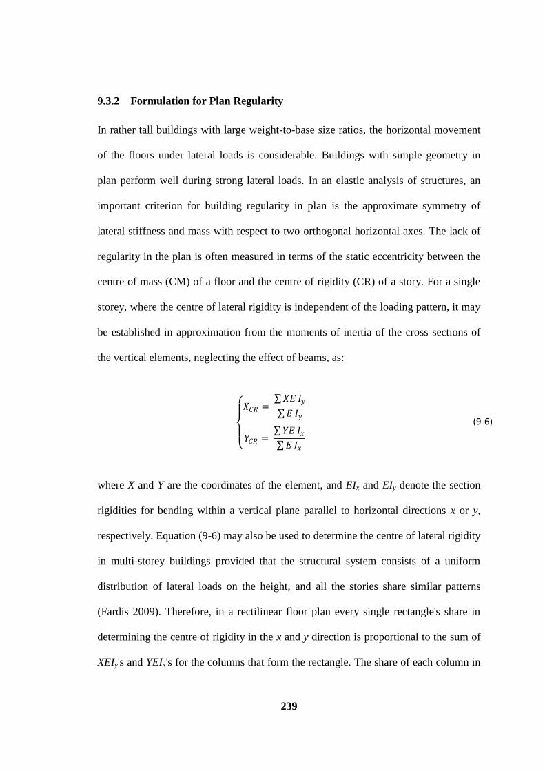
239
9.3.2 Formulation for Plan Regularity
In rather tall buildings with large weight-to-base size ratios, the horizontal movement
of the floors under lateral loads is considerable. Buildings with simple geometry in
plan perform well during strong lateral loads. In an elastic analysis of structures, an
important criterion for building regularity in plan is the approximate symmetry of
lateral stiffness and mass with respect to two orthogonal horizontal axes. The lack of
regularity in the plan is often measured in terms of the static eccentricity between the
centre of mass (CM) of a floor and the centre of rigidity (CR) of a story. For a single
storey, where the centre of lateral rigidity is independent of the loading pattern, it may
be established in approximation from the moments of inertia of the cross sections of
the vertical elements, neglecting the effect of beams, as:
𝑋𝐶𝑅 =
𝑋𝐸 𝐼𝑦 𝐸 𝐼𝑦
𝑌𝐶𝑅 = 𝑌𝐸 𝐼𝑥 𝐸 𝐼𝑥
(9-6)
where X and Y are the coordinates of the element, and EIx and EIy denote the section
rigidities for bending within a vertical plane parallel to horizontal directions x or y,
respectively. Equation (9-6) may also be used to determine the centre of lateral rigidity
in multi-storey buildings provided that the structural system consists of a uniform
distribution of lateral loads on the height, and all the stories share similar patterns
(Fardis 2009). Therefore, in a rectilinear floor plan every single rectangle's share in
determining the centre of rigidity in the x and y direction is proportional to the sum of
XEIy's and YEIx's for the columns that form the rectangle. The share of each column in
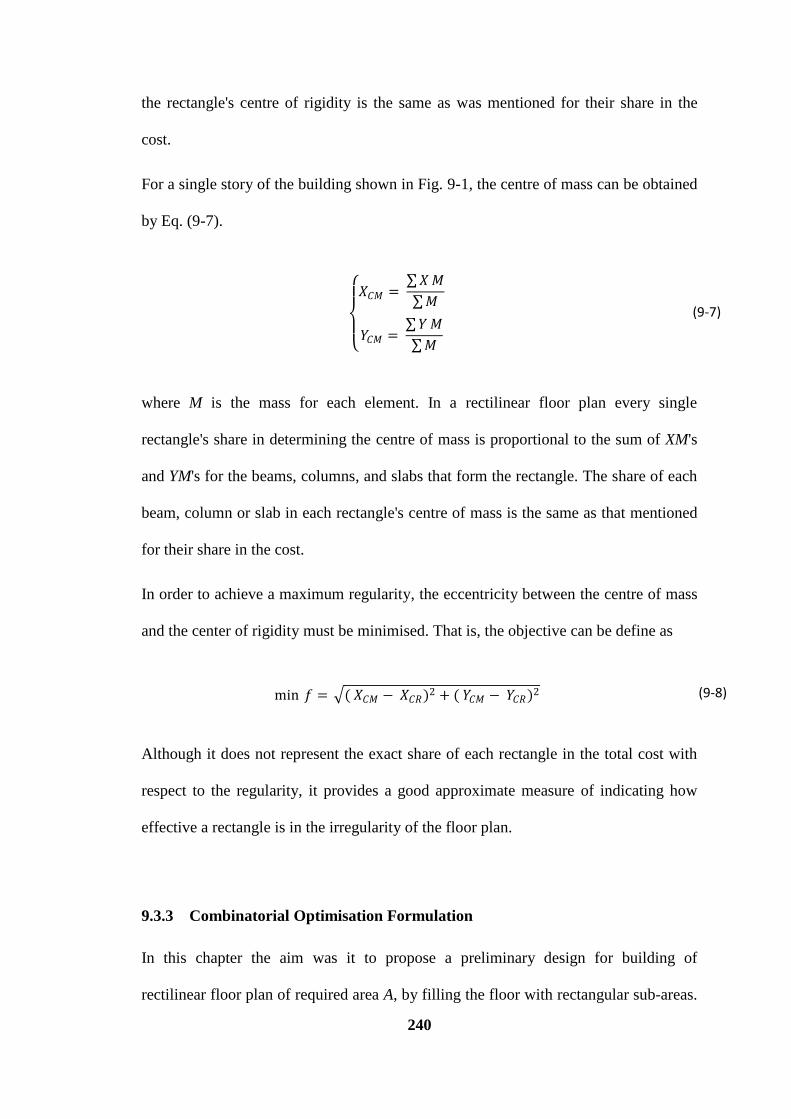
240
the rectangle's centre of rigidity is the same as was mentioned for their share in the
cost.
For a single story of the building shown in Fig. 9-1, the centre of mass can be obtained
by Eq. (9-7).
𝑋𝐶𝑀 =
𝑋 𝑀
𝑀
𝑌𝐶𝑀 = 𝑌 𝑀
𝑀
(9-7)
where M is the mass for each element. In a rectilinear floor plan every single
rectangle's share in determining the centre of mass is proportional to the sum of XM's
and YM's for the beams, columns, and slabs that form the rectangle. The share of each
beam, column or slab in each rectangle's centre of mass is the same as that mentioned
for their share in the cost.
In order to achieve a maximum regularity, the eccentricity between the centre of mass
and the center of rigidity must be minimised. That is, the objective can be define as
min 𝑓 = ( 𝑋𝐶𝑀 − 𝑋𝐶𝑅)2 + ( 𝑌𝐶𝑀 − 𝑌𝐶𝑅)2 (9-8)
Although it does not represent the exact share of each rectangle in the total cost with
respect to the regularity, it provides a good approximate measure of indicating how
effective a rectangle is in the irregularity of the floor plan.
9.3.3 Combinatorial Optimisation Formulation
In this chapter the aim was it to propose a preliminary design for building of
rectilinear floor plan of required area A, by filling the floor with rectangular sub-areas.
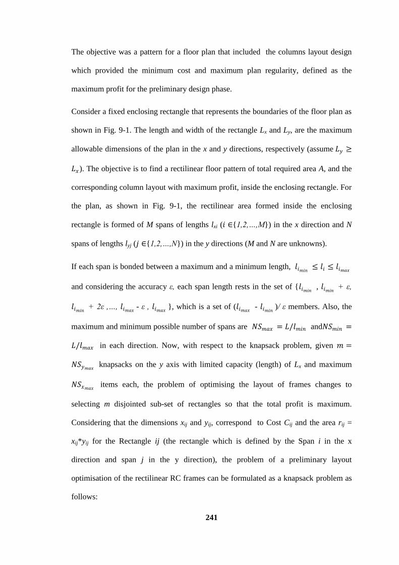
241
The objective was a pattern for a floor plan that included the columns layout design
which provided the minimum cost and maximum plan regularity, defined as the
maximum profit for the preliminary design phase.
Consider a fixed enclosing rectangle that represents the boundaries of the floor plan as
shown in Fig. 9-1. The length and width of the rectangle Lx and Ly, are the maximum
allowable dimensions of the plan in the x and y directions, respectively (assume 𝐿𝑦 ≥
𝐿𝑥 ). The objective is to find a rectilinear floor pattern of total required area A, and the
corresponding column layout with maximum profit, inside the enclosing rectangle. For
the plan, as shown in Fig. 9-1, the rectilinear area formed inside the enclosing
rectangle is formed of M spans of lengths lxi (𝑖 ∈{1,2,…,M}) in the x direction and N
spans of lengths lyj (𝑗 ∈{1,2,…,N}) in the y directions (M and N are unknowns).
If each span is bonded between a maximum and a minimum length, 𝑙𝑖𝑚𝑖𝑛≤ 𝑙𝑖 ≤ 𝑙𝑖𝑚𝑎𝑥
and considering the accuracy ε, each span length rests in the set of {𝑙𝑖𝑚𝑖𝑛 , 𝑙𝑖𝑚𝑖𝑛
+ ε,
𝑙𝑖𝑚𝑖𝑛 + 2ε ,…, 𝑙𝑖𝑚𝑎𝑥
- ε , 𝑙𝑖𝑚𝑎𝑥}, which is a set of (𝑙𝑖𝑚𝑎𝑥
- 𝑙𝑖𝑚𝑖𝑛)/ ε members. Also, the
maximum and minimum possible number of spans are 𝑁𝑆𝑚𝑎𝑥 = 𝐿/𝑙𝑚𝑖𝑛 and𝑁𝑆𝑚𝑖𝑛 =
𝐿/𝑙𝑚𝑎𝑥 in each direction. Now, with respect to the knapsack problem, given 𝑚 =
𝑁𝑆𝑦𝑚𝑎𝑥 knapsacks on the y axis with limited capacity (length) of Lx and maximum
𝑁𝑆𝑥𝑚𝑎𝑥 items each, the problem of optimising the layout of frames changes to
selecting m disjointed sub-set of rectangles so that the total profit is maximum.
Considering that the dimensions xij and yij, correspond to Cost Cij and the area rij =
xij*yij for the Rectangle ij (the rectangle which is defined by the Span i in the x
direction and span j in the y direction), the problem of a preliminary layout
optimisation of the rectilinear RC frames can be formulated as a knapsack problem as
follows:
242
𝑚𝑎𝑥 𝑓 = 𝑧𝑖𝑗
𝐶𝑖𝑗
n
i=1
m
j=1
(9-9)
𝑙𝑥𝑖𝑧𝑖𝑗
ni=1 ≤ 𝐿𝑥 𝑗 ∈ {1,2, … , 𝑚} (9-10)
𝑟𝑖𝑗 𝑧𝑖𝑗
n
i=1
𝑚
𝑗 =1
≤ A (9-11)
𝑧𝑖𝑗 = 1 𝑖𝑓 𝑟𝑒𝑐𝑡𝑎𝑛𝑔𝑙𝑒 𝑖 𝑖𝑠 𝑐𝑜𝑠𝑒𝑛 𝑓𝑜𝑟 𝑠𝑝𝑎𝑛 𝑗 0 𝑖𝑓 𝑟𝑒𝑐𝑡𝑎𝑛𝑔𝑙𝑒 𝑖 𝑖𝑠 𝑛𝑜𝑡 𝑐𝑜𝑠𝑒𝑛 𝑓𝑜𝑟 𝑠𝑝𝑎𝑛 𝑗
(9-12)
∀ 𝑖, 𝑗: 𝑦𝑖𝑗 = 𝑦(𝑖+1)𝑗 & 𝑥𝑖𝑗 = 𝑥𝑖(𝑗+1) (9-13)
Equation (9-9) is the objective function which aims to maximise the profit of the
layout design, and Equation (9-10), as a constraint, guarantees that the lengths do not
exceed the maximum permitted length in the x direction. As another constraint on the
total areas, Eq. (9-11) must be imposed onto the problem. Equation (9-12) is the basis
of the integer programming for the combinatorial problem, while Equation (9-13)
guaranties not to have off-centre columns, and all the columns in a level are in a row.
In case of other priorities, additional constraints can be added to the above mentioned
constraints. For example, if it is desired to have symmetry in the plan layout or in case
of a preference for any particular shape for the plan layout, or to avoid eccentricity
between the centre of mass and the centre of rigidity (to avoid torsion and comply with
the some design standards), or any other priorities over the design, there could be
constraints on the dimensions of the rectangles, the size of knapsacks, or the order of
knapsacks, in order to satisfy the constraints. In case of single or double symmetric
plans, half or a quarter of the plan can respectively be modelled by the knapsack
problem. Another optional constraint that can be imposed onto the problem is for not
letting the building be split into two or more separate parts. For this purpose, no
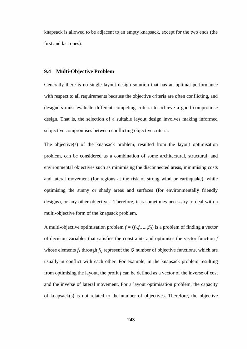
243
knapsack is allowed to be adjacent to an empty knapsack, except for the two ends (the
first and last ones).
9.4 Multi-Objective Problem
Generally there is no single layout design solution that has an optimal performance
with respect to all requirements because the objective criteria are often conflicting, and
designers must evaluate different competing criteria to achieve a good compromise
design. That is, the selection of a suitable layout design involves making informed
subjective compromises between conflicting objective criteria.
The objective(s) of the knapsack problem, resulted from the layout optimisation
problem, can be considered as a combination of some architectural, structural, and
environmental objectives such as minimising the disconnected areas, minimising costs
and lateral movement (for regions at the risk of strong wind or earthquake), while
optimising the sunny or shady areas and surfaces (for environmentally friendly
designs), or any other objectives. Therefore, it is sometimes necessary to deal with a
multi-objective form of the knapsack problem.
A multi-objective optimisation problem f = (f1,f2,…,fQ) is a problem of finding a vector
of decision variables that satisfies the constraints and optimises the vector function f
whose elements f1 through fQ represent the Q number of objective functions, which are
usually in conflict with each other. For example, in the knapsack problem resulting
from optimising the layout, the profit f can be defined as a vector of the inverse of cost
and the inverse of lateral movement. For a layout optimisation problem, the capacity
of knapsack(s) is not related to the number of objectives. Therefore, the objective
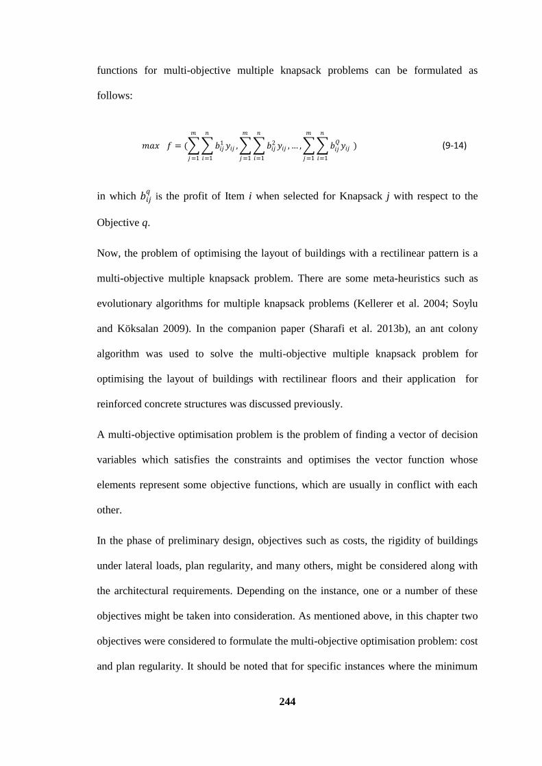
244
functions for multi-objective multiple knapsack problems can be formulated as
follows:
𝑚𝑎𝑥 𝑓 = ( 𝑏𝑖𝑗1 𝑦𝑖𝑗 ,
𝑛
𝑖=1
𝑚
𝑗 =1
𝑏𝑖𝑗2 𝑦𝑖𝑗 , … , 𝑏𝑖𝑗
𝑄𝑦𝑖𝑗
𝑛
𝑖=1
)
𝑚
𝑗 =1
𝑛
𝑖=1
𝑚
𝑗 =1
(9-14)
in which 𝑏𝑖𝑗𝑞
is the profit of Item i when selected for Knapsack j with respect to the
Objective q.
Now, the problem of optimising the layout of buildings with a rectilinear pattern is a
multi-objective multiple knapsack problem. There are some meta-heuristics such as
evolutionary algorithms for multiple knapsack problems (Kellerer et al. 2004; Soylu
and Köksalan 2009). In the companion paper (Sharafi et al. 2013b), an ant colony
algorithm was used to solve the multi-objective multiple knapsack problem for
optimising the layout of buildings with rectilinear floors and their application for
reinforced concrete structures was discussed previously.
A multi-objective optimisation problem is the problem of finding a vector of decision
variables which satisfies the constraints and optimises the vector function whose
elements represent some objective functions, which are usually in conflict with each
other.
In the phase of preliminary design, objectives such as costs, the rigidity of buildings
under lateral loads, plan regularity, and many others, might be considered along with
the architectural requirements. Depending on the instance, one or a number of these
objectives might be taken into consideration. As mentioned above, in this chapter two
objectives were considered to formulate the multi-objective optimisation problem: cost
and plan regularity. It should be noted that for specific instances where the minimum
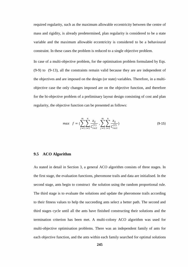
245
required regularity, such as the maximum allowable eccentricity between the centre of
mass and rigidity, is already predetermined, plan regularity is considered to be a state
variable and the maximum allowable eccentricity is considered to be a behavioural
constraint. In these cases the problem is reduced to a single objective problem.
In case of a multi-objective problem, for the optimisation problem formulated by Eqs.
(9-9) to (9-13), all the constraints remain valid because they are are independent of
the objectives and are imposed on the design (or state) variables. Therefore, in a multi-
objective case the only changes imposed are on the objective function, and therefore
for the bi-objective problem of a preliminary layout design consisting of cost and plan
regularity, the objective function can be presented as follows:
𝑚𝑎𝑥 𝑓 = ( 𝑧𝑖𝑗
𝐶𝑟𝑒𝑐𝑡(1)
,
𝑛
𝑖=1
𝑚
𝑗 =1
𝑧𝑖𝑗
𝐶𝑟𝑒𝑐𝑡(2)
)
𝑛
𝑖=1
𝑚
𝑗 =1
(9-15)
9.5 ACO Algorithm
As stated in detail in Section 3, a general ACO algorithm consists of three stages. In
the first stage, the evaluation functions, pheromone trails and data are initialised. In the
second stage, ants begin to construct the solution using the random proportional rule.
The third stage is to evaluate the solutions and update the pheromone trails according
to their fitness values to help the succeeding ants select a better path. The second and
third stages cycle until all the ants have finished constructing their solutions and the
termination criterion has been met. A multi-colony ACO algorithm was used for
multi-objective optimisation problems. There was an independent family of ants for
each objective function, and the ants within each family searched for optimal solutions
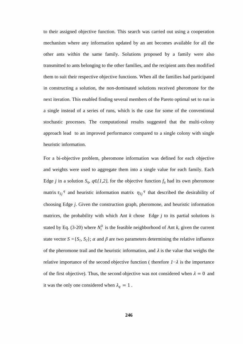
246
to their assigned objective function. This search was carried out using a cooperation
mechanism where any information updated by an ant becomes available for all the
other ants within the same family. Solutions proposed by a family were also
transmitted to ants belonging to the other families, and the recipient ants then modified
them to suit their respective objective functions. When all the families had participated
in constructing a solution, the non-dominated solutions received pheromone for the
next iteration. This enabled finding several members of the Pareto optimal set to run in
a single instead of a series of runs, which is the case for some of the conventional
stochastic processes. The computational results suggested that the multi-colony
approach lead to an improved performance compared to a single colony with single
heuristic information.
For a bi-objective problem, pheromone information was defined for each objective
and weights were used to aggregate them into a single value for each family. Each
Edge j in a solution Sq, q∈{1,2}, for the objective function fq had its own pheromone
matrix 𝜏𝑆𝑗𝑞 and heuristic information matrix 𝜂𝑆𝑗
𝑞 that described the desirability of
choosing Edge j. Given the construction graph, pheromone, and heuristic information
matrices, the probability with which Ant k chose Edge j to its partial solutions is
stated by Eq. (3-20) where 𝑁𝑖𝑘 is the feasible neighborhood of Ant k, given the current
state vector S ={S1, S2}; 𝛼 and β are two parameters determining the relative influence
of the pheromone trail and the heuristic information, and 𝜆 is the value that weighs the
relative importance of the second objective function ( therefore 1−𝜆 is the importance
of the first objective). Thus, the second objective was not considered when 𝜆 = 0 and
it was the only one considered when 𝜆𝑞 = 1 .
247
In the multiple ACO algorithms the set of weight vectors that each colony applied in
order to aggregate its multiple pheromone information represents a region in the
objective space on which the colony focussed the search. In multi-objective problems,
as in single objective ones, the iteration-best or best-so-far strategy can be used to
update the pheromone by taking the best solutions from a candidate set, including all
solutions found in the current iteration, or since the start of the algorithm. In this case
the straight forward criterion was the Pareto optimality and thus the best solutions of
the candidate set weree those that were non-dominated, or in other words, those
solutions that belong to the Pareto set. As each objective defines the solution
components in a different way, the selected solutions update each pheromone matrix
differently because each solution component has its own meaning for every
pheromone matrix. In this strategy, only the best solutions with respect to each
objective were selected to update the pheromone information. Then, each pheromone
matrix, associated with each objective, was updated by the solution with the best
objective value for the corresponding objective. Therefore, the minimum number of
ants allowed to update the pheromone information in a colony is equal to the number
of objectives. Since an ant cannot update the pheromone information of more than one
colony, each pheromone matrix focuses on one objective, thus the aggregation of all of
them by means of a weight vector regulates the relative importance of each objective.
In the pheromone updating stage of the bi-objective ACO, some special care must be
taken to guarantee an acceptable convergence. When depositing pheromone the only
restriction is that the total solution cost cannot be used for this purpose because the
values of different objective functions are not comparable, and the amount of
pheromone deposited must be independent for each family, otherwise some objectives
are implicitly considered more important than others. With regards to the procedure

248
for evaporating pheromone, any method can be used although efficient techniques are
preferred
The general form of the geometric layout optimisation problem for RC rectilinear
buildings that were represented by a bi-objective knapsack problem can be dealt with
using ACO algorithms. The bi-objective ACO algorithm proposed for this problem is
a Max-Min Ant System (MMAS) algorithm (Stutzle and Hoos 1997), performed in the
following steps:
Stage 1- Initialise Data: In this stage, and before starting the iterative part of the
algorithm, the required data is initialised as follows:
Read instance: The mechanical properties of the materials involved and their relative
costs, building information such as its maximum dimensions, the area required, the
maximum and minimum span lengths, and the accuracy needed, must be defined.
Having the required information the number of knap knapsacks m and the their
capacity can be determined.
Build a construction graph: A construction graph is formed of m sub-graphs, where
each represents a knapsack. The profit of adding items (rectangles) is associated with a
sub-graph rather than edges or nodes. In other words, each sub-graph determines the
profit of a rectangle. Fig. 9-2 shows how this graph is formed. Each rectangle is
represented by a sub-graph which is formed from three layers: first, a set representing
the width (ly), second by a set representing the length (lx), and the third layers that
determines if the selected rectangle of width ly and length lx is a void or a filled
rectangle. The entire construction graph is formed from m sub-graphs where each one
represents a knapsack. In order to satisfy Eq. (9-13) and avoid the off-centre columns,
the Sub-graphs 2 to m, which represent Knapsacks 2 to m, can be simplified. To that
249
end, since all the rectangles zij with the same j have identical lengths, it is only
necessary for Knapsacks 2 to m to determine their widths in each iteration. Therefore,
Sub-graphs 2 to m can be reduced to one set of layers one and three, as shown in Fig.
9-3.
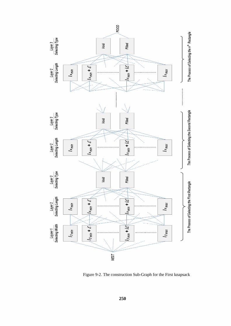
250
Figure 9-2. The construction Sub-Graph for the First knapsack
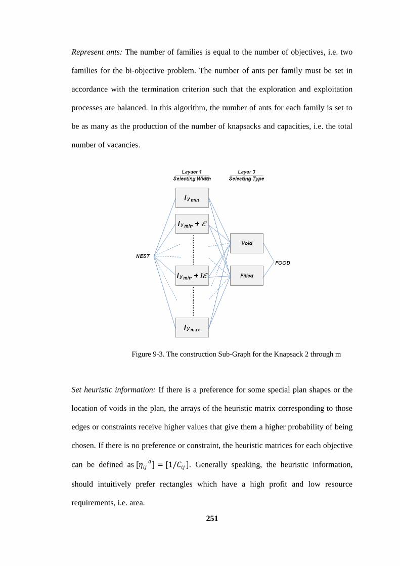
251
Represent ants: The number of families is equal to the number of objectives, i.e. two
families for the bi-objective problem. The number of ants per family must be set in
accordance with the termination criterion such that the exploration and exploitation
processes are balanced. In this algorithm, the number of ants for each family is set to
be as many as the production of the number of knapsacks and capacities, i.e. the total
number of vacancies.
Figure 9-3. The construction Sub-Graph for the Knapsack 2 through m
Set heuristic information: If there is a preference for some special plan shapes or the
location of voids in the plan, the arrays of the heuristic matrix corresponding to those
edges or constraints receive higher values that give them a higher probability of being
chosen. If there is no preference or constraint, the heuristic matrices for each objective
can be defined as [𝜂𝑖𝑗𝑞 ] = [1/𝐶𝑖𝑗 ]. Generally speaking, the heuristic information,
should intuitively prefer rectangles which have a high profit and low resource
requirements, i.e. area.
252
Set parameters: Parameters such as α, β and 𝜆, which determine the relative influence
of the pheromone trail, the heuristic information, and the relative importance of each
objective function, are determined. The evaporation rate ρ ∈ (0, 1] is defined for all
colonies. In this algorithm, the parameters α, β and ρ are considered constant for all
objectives. For MMAS, useful hints for defining efficient values for α, β and ρ can be
found in (Dorigo 2006).
Initialize pheromone trails: MMAS limits the possible range of pheromone trail
values to the interval [τq
min, τq
max]. Also, the pheromone trails are initialised to the
upper pheromone trail limit, which, together with a small rate of pheromone
evaporation, increases the exploration of tours at the start of the search (Dorigo and
Stützle 2004). As a good estimation, the lower level is set to be τq
min= τq
max /a, where a
is a parameter that can be calculated based on the quality of solutions (Stutzle and
Hoos 1997).
Stage 2- Construct Ants Solutions: The stage of constructing a solution continues
iteratively until the termination criterion has been met. There is no general termination
criterion applicable for all ACO algorithms. Depending on the optimisation problem,
some criteria such as the maximum CPU time, the maximum number of solutions
generated, the percentage deviation from a lower/upper bound from the optimum, and
the maximum number of iterations without an improvement in the quality of the
solution, or a combination of them, can be set as the termination criterion. This stage
of the algorithm is performed as follows:
Empty ant's memory: All the edges and nodes of the graph are marked as unselected.

253
Place ants on initial positions: For the bi-objective knapsack problem, two ants are
allocated to each node: one ant belongs to the cost minimisation family and the other
to the plan regularity maximisation family.
Construct solutions: Ants start constructing their solutions independently using Eq. (3-
19). To construct trails for each problem the ants must comply with the corresponding
constraints. In this phase the constraints imposed, such as geometrical constraints on
selecting rectangles to avoid off-centre columns, as given by Eq. (9-13), restrict the
ants' solutions. The solution construction must also consider the knapsack constraints
given by Eq. (9-11). This can only be done during the process of constructing a
solution by allowing ants to add only those components that, when added to their
current partial solution, do not violate any knapsack or the total area required. Each
ant iteratively adds rectangles in a probabilistic way that is biased by pheromone trails
and heuristic information, but as long as the selected rectangles meet the constraints,
each item can be added as many times as required. An ant's solution construction ends
if no item can be added anymore without violating any of the constraints.
Save solutions information: The costs for all solution are explored, and the best-so-far
and iteration-best solution solutions for each family are determined.
Stage 3- Update Pheromone Trails :The bi-objective knapsack problem has a
particularity in that the pheromone trails are only associated with rectangles and refer
to the desirability of adding the rectangle to the current vacant position in a knapsack.
An iterative pheromone update continues until the termination criterion has been met.
This stage is performed in two steps as follows:
Pheromone evaporation: The pheromone evaporation on all edges and for all
objectives is implemented by:
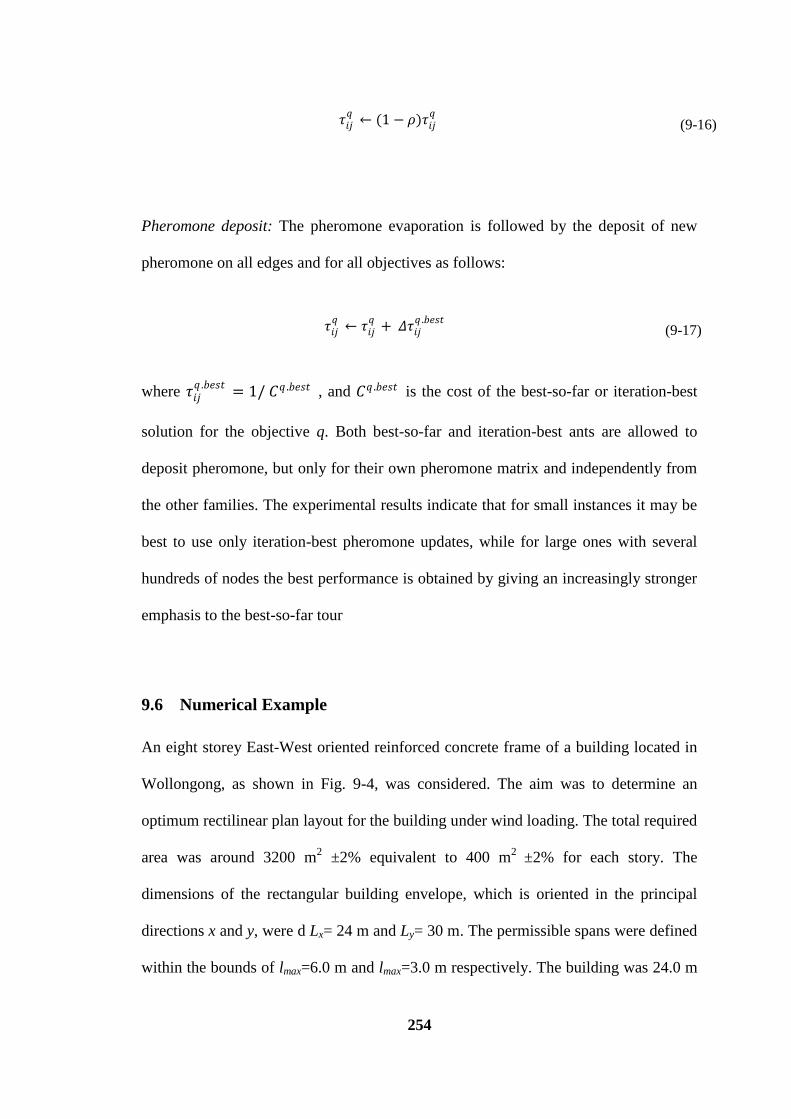
254
𝜏𝑖𝑗𝑞
← (1 − 𝜌)𝜏𝑖𝑗𝑞
(9-16)
Pheromone deposit: The pheromone evaporation is followed by the deposit of new
pheromone on all edges and for all objectives as follows:
𝜏𝑖𝑗𝑞
← 𝜏𝑖𝑗𝑞
+ 𝛥𝜏𝑖𝑗𝑞 .𝑏𝑒𝑠𝑡
(9-17)
where 𝜏𝑖𝑗𝑞 .𝑏𝑒𝑠𝑡 = 1/ 𝐶𝑞 .𝑏𝑒𝑠𝑡 , and 𝐶𝑞 .𝑏𝑒𝑠𝑡 is the cost of the best-so-far or iteration-best
solution for the objective q. Both best-so-far and iteration-best ants are allowed to
deposit pheromone, but only for their own pheromone matrix and independently from
the other families. The experimental results indicate that for small instances it may be
best to use only iteration-best pheromone updates, while for large ones with several
hundreds of nodes the best performance is obtained by giving an increasingly stronger
emphasis to the best-so-far tour
9.6 Numerical Example
An eight storey East-West oriented reinforced concrete frame of a building located in
Wollongong, as shown in Fig. 9-4, was considered. The aim was to determine an
optimum rectilinear plan layout for the building under wind loading. The total required
area was around 3200 m2 ±2% equivalent to 400 m
2 ±2% for each story. The
dimensions of the rectangular building envelope, which is oriented in the principal
directions x and y, were d Lx= 24 m and Ly= 30 m. The permissible spans were defined
within the bounds of lmax=6.0 m and lmax=3.0 m respectively. The building was 24.0 m
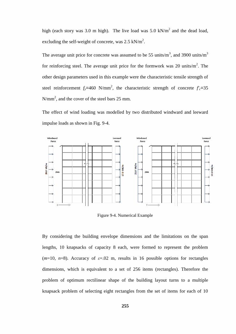
255
high (each story was 3.0 m high). The live load was 5.0 kN/m2 and the dead load,
excluding the self-weight of concrete, was 2.5 kN/m2.
The average unit price for concrete was assumed to be 55 units/m3, and 3900 units/m
3
for reinforcing steel. The average unit price for the formwork was 20 units/m2. The
other design parameters used in this example were the characteristic tensile strength of
steel reinforcement fy=460 N/mm2, the characteristic strength of concrete f'c=35
N/mm2, and the cover of the steel bars 25 mm.
The effect of wind loading was modelled by two distributed windward and leeward
impulse loads as shown in Fig. 9-4.
Figure 9-4. Numerical Example
By considering the building envelope dimensions and the limitations on the span
lengths, 10 knapsacks of capacity 8 each, were formed to represent the problem
(m=10, n=8). Accuracy of ε=.02 m, results in 16 possible options for rectangles
dimensions, which is equivalent to a set of 256 items (rectangles). Therefore the
problem of optimum rectilinear shape of the building layout turns to a multiple
knapsack problem of selecting eight rectangles from the set of items for each of 10
256
knapsacks such that the total area of the rectangles does not exceed 400 m2
±2% and
the profit is a maximum.
As a primary design for a proposed ACO algorithm, a rectangular layout of 4 identical
spans in each direction was defined. The initial solution and the knapsacks
corresponding to the problem and the primary solution are displayed in Fig 9-5. It
should be added that every initial design based on the preliminary judgment of the
designer and/or using approximate charts or formulae which meet the design standard
requirements, can be used as the initial design and as the starting point of optimisation
process. Based on the above mentioned primary design, the primary cost of the
structure was equal to 976991 units.
Figure 9-5. Numerical Example: Initial plan design and the corresponding Knapsacks
To determine the costs in this example, three control sections were selected for every
member: two ends and one in the middle. Determining benefits related to costs and
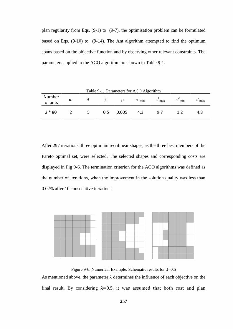
257
plan regularity from Eqs. (9-1) to (9-7), the optimisation problem can be formulated
based on Eqs. (9-10) to (9-14). The Ant algorithm attempted to find the optimum
spans based on the objective function and by observing other relevant constraints. The
parameters applied to the ACO algorithm are shown in Table 9-1.
Table 9-1. Parameters for ACO Algorithm
Number of ants
α Β 𝜆 ρ τ1
min τ1
max τ2
min τ2
max
2 * 80 2 5 0.5 0.005 4.3 9.7 1.2 4.8
After 297 iterations, three optimum rectilinear shapes, as the three best members of the
Pareto optimal set, were selected. The selected shapes and corresponding costs are
displayed in Fig 9-6. The termination criterion for the ACO algorithms was defined as
the number of iterations, when the improvement in the solution quality was less than
0.02% after 10 consecutive iterations.
Figure 9-6. Numerical Example: Schematic results for 𝜆=0.5
As mentioned above, the parameter 𝜆 determines the influence of each objective on the
final result. By considering 𝜆=0.5, it was assumed that both cost and plan
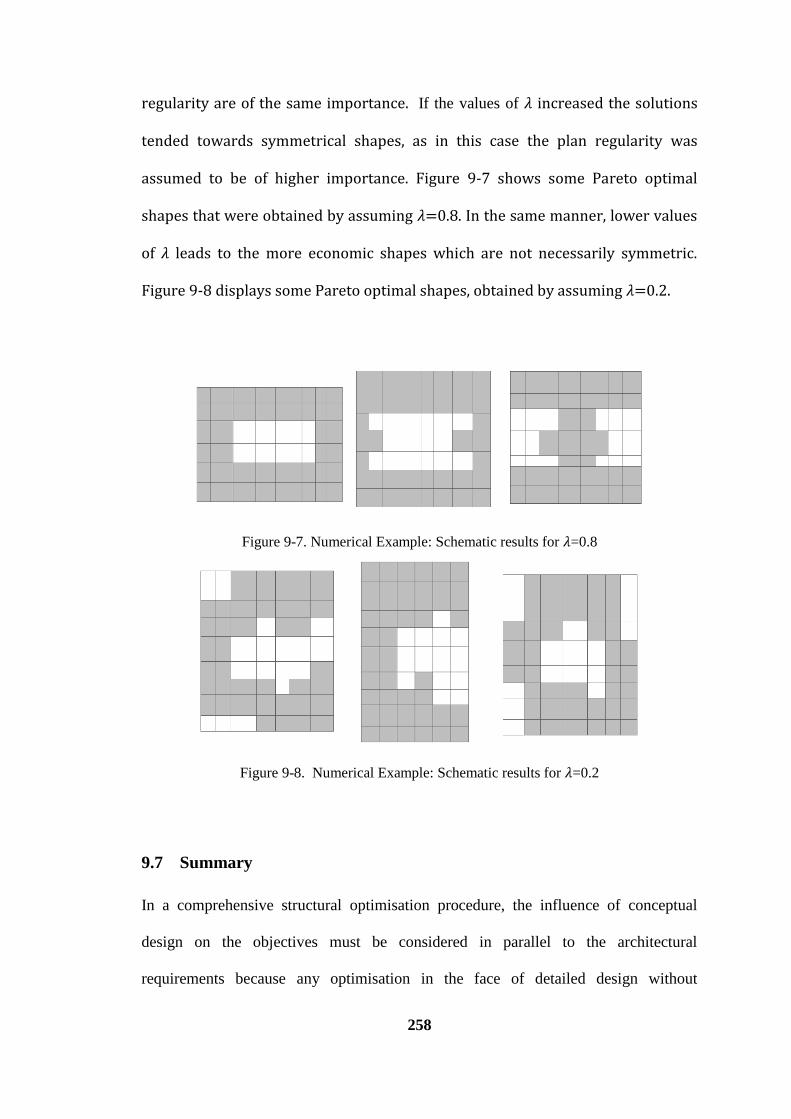
258
regularity are of the same importance. If the values of 𝜆 increased the solutions
tended towards symmetrical shapes, as in this case the plan regularity was
assumed to be of higher importance. Figure 9-7 shows some Pareto optimal
shapes that were obtained by assuming 𝜆=0.8. In the same manner, lower values
of 𝜆 leads to the more economic shapes which are not necessarily symmetric.
Figure 9-8 displays some Pareto optimal shapes, obtained by assuming 𝜆=0.2.
Figure 9-7. Numerical Example: Schematic results for 𝜆=0.8
Figure 9-8. Numerical Example: Schematic results for 𝜆=0.2
9.7 Summary
In a comprehensive structural optimisation procedure, the influence of conceptual
design on the objectives must be considered in parallel to the architectural
requirements because any optimisation in the face of detailed design without

259
considering the effect of the conceptual design will not lead to a globally optimum
result. Over the last few decades, combinatorial optimisation has experienced a fast
development because a lot of problems in combinatorial optimisation arose directly
from everyday practice in engineering and management. In This chapter, an automated
combinatorial technique was presented for a preliminary layout optimisation of framed
buildings with rectilinear patterns. The method supports all the buildings with
rectilinear shapes where the number and size of spans and the shape of the plan can be
considered as variables. To that end, the knapsack problem as a basic applied
combinatorial optimisation problem was used.
The objective was to find layouts of maximum profit for frames with a rectilinear
pattern that also satisfied the dimensional constraints imposed. The term profit is a
general term that can be referred to any objective such as cost minimisation, optimum
serviceability, energy efficiency, or any other objectives and/or a combination of them
in the phase of preliminary design. To that end, some variations of knapsack problems
were considered and a geometric layout optimisation of rectilinear framed buildings of
different conditions were treated as a suitable knapsack problem. The method was
presented in a general form and was not confined to optimisation under a certain type
of action effect and/or geometrical constraints.
Then, by applying the combinatorics approach, a bi-objective ACO algorithm was
proposed for a preliminary layout optimisation. The method was applied to the
conceptual design of RC buildings to achieve an optimum plan layout of rectilinear
shape for RC frames. The objectives were minimum cost and maximum plan
regularity (minimum eccentricity between the floor centre of mass and the storey
centre of lateral stiffness). The numerical example demonstrates the robustness of the
approach and shows that the methodology, with the help of the proposed ACO

260
algorithm, can easily be carried out to simplify the computer-aided preliminary layout
design of RC frames
.
261
10 Conclusion
The phase of preliminary layout design, is usually carried out based on the
architectural requirements. While a practical preliminary layout design, must satisfy
the architectural constraints, it must also consider the profit achieved. This thesis
developed a methodology that helps the designer to select the most economic and
profitable layout designs among the possible ones that in parallel satisfy the
architectural constraints.
A challenging issue at the beginning stage of this thesis was, in automated layout
optimisation problems, it is quite difficult to efficiently represent the layout of the
structure so that it could account for all the relevant objectives and costs. Multiple
objectives that were considered for a structure, such as cost and plan regularity, in the
preliminary design phase could make it too difficult to achieve a global optimum, if
the problem was dealt with in the traditional space. The reason is, optimisation can be
applied to clearly defined mathematical problems and smooth search spaces. Yet, the
conceptual design of RC structures usually lacks such features, at least for some of the
objectives because some objectives and constraints are often changed during the
design process. On the other hand, variables arising from multiple objectives such as
the cost variables, in combination with layout variables for a large structure, could
make the optimisation problem quite complicated.
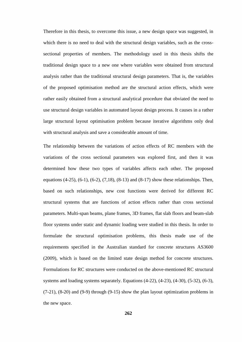
262
Therefore in this thesis, to overcome this issue, a new design space was suggested, in
which there is no need to deal with the structural design variables, such as the cross-
sectional properties of members. The methodology used in this thesis shifts the
traditional design space to a new one where variables were obtained from structural
analysis rather than the traditional structural design parameters. That is, the variables
of the proposed optimisation method are the structural action effects, which were
rather easily obtained from a structural analytical procedure that obviated the need to
use structural design variables in automated layout design process. It causes in a rather
large structural layout optimisation problem because iterative algorithms only deal
with structural analysis and save a considerable amount of time.
The relationship between the variations of action effects of RC members with the
variations of the cross sectional parameters was explored first, and then it was
determined how these two types of variables affects each other. The proposed
equations (4-25), (6-1), (6-2), (7,18), (8-13) and (8-17) show these relationships. Then,
based on such relationships, new cost functions were derived for different RC
structural systems that are functions of action effects rather than cross sectional
parameters. Multi-span beams, plane frames, 3D frames, flat slab floors and beam-slab
floor systems under static and dynamic loading were studied in this thesis. In order to
formulate the structural optimisation problems, this thesis made use of the
requirements specified in the Australian standard for concrete structures AS3600
(2009), which is based on the limited state design method for concrete structures.
Formulations for RC structures were conducted on the above-mentioned RC structural
systems and loading systems separately. Equations (4-22), (4-23), (4-30), (5-32), (6-3),
(7-21), (8-20) and (9-9) through (9-15) show the plan layout optimization problems in
the new space.
263
Another obstacle in the way of optimising the cost of preliminary layout design was
architectural constraints, and having to convince architects to make changes so that the
optimum column layout can be accommodated in the proposed architectural plan. In
fact, in most cases engineers must follow the architectural plan. Architects intend to
locate the columns in their desired locations, say by hiding them at the intersections of
walls, regardless of whether or not they are in their optimum locations.
Such an obstacle was addressed as follows. In practice, architects usually have some
discretion in choosing layout plans that meet their architectural requirements. In an
automated design procedure, they often try many conceptual designs and then select
one of them as the final plan. On the other hand, if architects selected layouts from the
Pareto-Optimal set, proposed by the combinatorial approach in this thesis, it would
allow them to choose a design which is close their conceptual design and allow an
economical conceptual design to be selected. On the other hand, such multi-objective
structural optimisation technique provides a useful tool for engineers and architects
who are interested in exploring structurally efficient forms and shapes during the
conceptual design stage of a project. This thesis, have addressed the problem by
proposing a set of optimum solution rather than an absolute global solution, which
might limit the architects. Moreover, minor changes in the plan layout, say the location
of walls and columns, in order to meet engineering requirements, are usually quite
acceptable to architects. The outcomes of the methodology developed in this thesis
show that even minor changes in the column layout can have a considerable effect on
costs. Therefore, in such cases, instead of a globally optimum column layout, a local
optimum column layout can be selected that meets the architects‘ requirements. This
thesis presents some mathematical relations showing how these changes affect the
cost. It can simplify the architectural decision making to select a near global design.
264
In fact the outcome of the thesis can be considered as criterion which can help the
designer to choose the most economic option. In order to select the most economical
plan among various layouts that satisfies architectural requirements, one needs to take
advantages of the reciprocal effects of cost factors and layout variables, suggested in
this study, which simultaneously considers the cost and layout.
To solve the structural optimization arising from the layout optimization of RC
structures, a large number of feasible options were examined during the conceptual
design process. When it comes to choosing an appropriate design among a huge
number of possible options and dimensions, the result is a large combinatorial
optimisation problem. Ant Colony Optimisation (ACO) has proved to provide strong
stochastic algorithms to deal with large combinatorial optimisations. In this thesis,
ACO algorithms were used to solve the combinatorial optimisation problems arising
from the layout optimisations problem. ACO algorithms have two advantages, positive
feedback that leads to a rapid discovery of good solutions, and distributed computation
that avoids premature convergence. When optimising the layout of RC structures,
taking advantage of heuristic information (heuristic matrix), ACO gives us the
opportunity to take many architectural or other priorities into account during this
process. That is, any desired plan layout and shape can be considered to be a priority
by defining appropriate heuristic information for the algorithm. The results of solved
numerical examples, as provided in this thesis, demonstrate that ACO is a suitable
method for such problems.
The outcomes of solved numerical examples show that using the methodology can
save up to 16 per cent in cost (depending on the instance), compared to designs which
have not been optimised for layout. This is a considerable cost saving that can bring a
significant improvement to the first step of a comprehensive design procedure. Indeed

265
the fact that all the architectural requirements and desired shapes and layouts can be
considered in this method, the value of the methodology proposed in this study
becomes very clear.
In future, such a methodology can be used for to optimise the shape and topology of
RC or the composite structures of various shapes. There is excellent potential for
further research in this field in respect to working on innovative shapes and form
finding for RC or composite structures, rather than being confined to rectangular or
rectilinear shapes, as well as considering other objectives such as energy saving and
maintenance.
266
References
Abachizadeh, M. and Tahani, M. (2009). "An ant colony optimization approach to
multi-objective optimal design of symmetric hybrid laminates for maximum
fundamental frequency and minimum cost." Structural and Multidisciplinary
Optimization 37(4): 367-376.
Abendroth, R. E. and Salmon, C. G. (1986) Sensitivity study of optimum RC
restrained end T-sections. Journal of Structural Engineering, ASCE, 112(8), 1928–
1943.
Achtziger, W. and Kočvara, M. (2007). "On the maximization of the fundamental
eigenvalue in topology optimization." Structural and Multidisciplinary Optimization
34(3): 181-195.
Achtziger, W. and Kočvara, M. (2007). "On the maximization of the fundamental
eigenvalue in topology optimization." Structural and Multidisciplinary Optimization
34(3): 181-195.
ACI-Committee-318 (2008). Building code requirements for structural concrete (ACI
318-08) and commentary. USA, American Concrete Institute
Adams, V. and Askenazi, A. (1999). Building better products with finite element
analysis, OnWord Press.
Adamu, A. and Karihaloo, B. L. (1995a) Minimum cost design of RC beams with
segmentation using continuum-type optimality criteria. Structural Optimization,
9(3/4), 220–235.
Adamu, A. and Karihaloo, B. L. (1995b) Minimum cost design of RC frames using
the DCOC method. Part I: columns under uniaxial bending actions. Structural
Optimization, 10(1), 16–32.
Adamu, A. and Karihaloo, B. L. (1995c) Minimum cost design of RC frames using the
DCOC method. Part II: columns under biaxial bending actions. Structural
Optimization, 10(1), 33–39.
Adamu, A., Karihaloo, B. L. and Rozvany, G. I. N. (1994) Minimum cost design of
reinforced concrete beams using continuum-type optimality criteria. Structural
Optimization, 7(1/2), 91–102.
Adeli, H. and Sarma, K. (2006). Cost optimization of structures: fuzzy logic, genetic
algorithms, and parallel computing, Wiley.
Ali NBH, Sellami M, Decelle AFC, Mangin JC (2009) Multi-stage production cost
optimization of semi-rigid steel frames using genetic algorithms. Engineering
Structures 31: 2766_2778
Al-Salloum Y. A. and Siddiqi G. H. (1994) Cost-optimum design of reinforced
concrete beams. ACI Structural Journal, 91(6), 647–655.
Amir, O., Bendsøe, M. P. and Sigmund, O. (2009). "Approximate reanalysis in
topology optimization." International Journal for Numerical Methods in Engineering
78(12): 1474-1491.
Anderson, K. E. and Chong, K. P. (1986) Least cost computer-aided design of steel
girders. Engineering Journal, AISC, Fourth Quarter, 151–156.
Annamalai, N., Lewis, A. D. M. and Goldberg, J. E. (1972) Cost optimization of
welded plate girders. Journal of the Structural Division, ASCE, 98(ST10), 2235–2246.
267
Arciszewski, Tomasz; Bloedorn, Eric; Michalski, Ryszard S.; Mustafa, Mohamad;
Wnek, Janusz, (1994), Machine learning of design rules: methodology and case study,
ASCE Journal of Computing in Civil Engineering, v 8 n 3, Jul, p 286-308.
Arora, J. S. (1989). Introduction to Optimum Design. Singapore, McGraw-Hill Book
Company.
AS/NZS1170.2 (2011). Structural design actions Part 2: Wind actions. Australia/New
Zealand, Standards Australia Limited.
AS3600 (2009). Concrete structures. Sydney, Standards Association of Australia.
Ashworth, A. (2004). Cost studies of buildings, Pearson Prentice Hall.
Attwater, I.J.S.; Anderson, J.; Findlay, G.E., (1993), Expert system application
combining disparate software to form an integrated pressure vessel design system,
Eighth International Conference on Applications of Artificial Intelligence in
Engineering, Toulouse, France, p 161-173.
Baker, Nelson C.; Fenves, Steven J., (1989), Towards a grammar for structural design,
Sixth Conference on Computing in Civil Engineering, Sep 11-13, Atlanta, GA, USA,
p 178-185.
Balachandran, M. and Gero, J. S. (1987). "Dimensioning of architectural floor plans
under conflicting objectives." Environment and Planning B: Planning and Design
14(1): 29-37.
Balling, R. J. and Yao, X. (1997). "Optimization of Reinforced Concrete Frames."
Journal of Structural Engineering 123(2): 193-202.
Barbarosie, C. and Toader, A.-M. (2010a). "Shape and topology optimization for
periodic problems." Structural and Multidisciplinary Optimization 40(1): 393-408.
Barbarosie, C. and Toader, A.-M. (2010b). "Shape and topology optimization for
periodic problems Part I: The shape and the topological derivative." Structural and
Multidisciplinary Optimization 40(1): 381-391.
Beckers M, Fleury C. (1997), Topology optimization involving discrete variables. In:
Gutkowski W, Mroz Z (eds) Proc. Second World Congress of Structural and
Multidisciplinary Optimization. Inst. Fundum. Techn. Res.,Warsaw
Belamaric, Igor; Cudina, Predrag; Ziha, Kalman, (1999), Design analysis of a new
generation of Suezmax tankers, Journal of Ship Production, v 15 n 1, Feb, Society of
Naval Architects and Marine Engineers, Jersey City, NJ, USA, p53-64.
Bendse MP. (1995), Optimization of structural topology, shape, and material.
Springer, Berlin.
Bendsøe, M. P. and Sigmund, O. (2003a). Topology Optimization: Theory, Methods,
and Applications, Springer.
Bendsøe, M. P. and Sigmund, O. (2003b). Topology optimization: theory, methods,
and applications Part II: optimization algorithm and numerical examples, Springer.
Bendsoe, M.P. (1989). Optimal shape design as a material distribution problem.
Struct. Optim. 1: 193–202.
Bendsoe, M.P. (1995). Optimization of Structural Topology, Shape and Material.
Berlin: Springer.
Bendsoe, M.P. and Kikuchi, N. (1988). Generating optimal topologies in structural
design using a homogenization method. Comput. Meth. Appl. Mech. Engng. 71: 197–
224.
268
Bendsoe, M.P. and Sigmund, O. (2003). Topology Optimization: Theory, Method and
Application, Berlin: Springer.
Blachut, J. and Eschenauer, H. A. (2001). Emerging Methods for Multidisciplinary
Optimization, Springer.
Borkowski, A.; Fleischmann, N.; Bletzinger, K.U., 1991, Supporting conceptual
decisions in structural design, Second International Conference on the Application of
Artificial Intelligence to Civil and Structural Engineering, Sep 3-5, Edinburgh, UK, p
87-96.
Bos, A.H.W., (1998), Aircraft conceptual design by genetic/gradient-guided
optimization, Engineering Applications of Artificial Intelligence, v 11 n 3, Jun,
Elsevier Science Ltd, Exeter, England, p 377-382.
Broersma, H. J. (2002). "On some intriguing problems in hamiltonian graph theory—a
survey." Discrete Mathematics 251(1–3): 47-69.
Brown, R. H. (1975) Minimum cost selection of one-way slab thickness. Journal of
the Structural Division, ASCE, 101(ST12), 2585–2590.
BS8110, B. S.-. (1997). Structural use of concrete, part 1, code of practice for design
and construction. London, British Standards Institution.
Building code requirements for structural concrete (ACI 318) and commentary (ACI
318R-02). Detroit (USA): American Concrete Institute; 2002.
Burnett, David; Rehder, Joe, (1994), Computational techniques enhance vehicle
design, Aerospace America, v 32 n 2, Feb, p 40-41.
Burns, S. A. (2002). Recent advances in optimal structural design, American Society
of Civil Engineers.Structural Engineering Institute. Technical Committee on Optimal
Structural Design.
Burns, S. A. and Design, S. E. I. T. C. O. O. S. (2002). Recent advances in optimal
structural design, American Society of Civil Engineers.
Cagan, Jonathan; Mitchell, William J., (1993), Shape annealing approach to creative
design of structures, 5th International Conference on Computing in Civil and Building
Engineering, Jun 7-9, New York, NY, USA, p 1642-1646.
Camp, C. V., Bichon, B. J. and Stovall, S. P. (2005). "Design of Steel Frames Using
Ant Colony Optimization." Journal of Structural Engineering 131(3): 369-379.
Capps, Stephen, (1994), New airlock approach for human exploration, 4th
International Conference on Engineering, Construction, and Operations in Space, Feb
26-Mar 03, Albuquerque, NM, USA, p 206-216.
Chamberlain, D.A., (1989), Aids for the conceptual design of prestressed membrane
structures, Proceedings of the Fourth International Conference on Civil and Structural
Engineering Computing, CIVIL-COMP, Sep 19-21, London, UK, p 15-20.
Chang, K.-H., Choi, K. K., Tsai, C.-S., Chen, C.-J., Choi, B. S. and Yu, X. (1995).
"Design Sensitivity Analysis and Optimization tool (DSO) for shape design
applications." Computing Systems in Engineering 6(2): 151-175.
Chen, Y. and Feng, J. (2012). "Generalized Eigenvalue Analysis of Symmetric
Prestressed Structures Using Group Theory." Journal of Computing in Civil
Engineering 26(4): 488-497.
Cheng, F. Y. and Li, D. (1997). "Multi-objective optimization design with Pareto
genetic algorithm." Journal of Structural Engineering 123(9): 1252.
269
Chew, M.; Kumar, P., (1993), Conceptual design of deployable space structures from
the viewpoint of symmetry, International Journal of Space Structures, v 8 n 1-2, p 17-
27.
Chinowsky, Paul S., (1996), ICeD: An Interdisciplinary Conceptual Design
Environment, Computing in Civil Engineering (New York), p 133-139.
Chinowsky, Paul S.; Reinschmidt, Kenneth F., (1995), Qualitative geometric reasoner
for integrated design, Proceedings of the 2nd ASCE Congress on Computing in Civil
Engineering, Jun 5-8, Atlanta, GA, USA, p 1332-1339.
Chirehdast, M.; Ambo, S.D., (1995), Topology optimization of planar cross-sections,
Structural Optimization, v9 n3-4, Jul, p 266-268.
Choi, K. K. and Kim, N. H. (2005). Structural Sensitivity Analysis and Optimization:
Linear systems, Springer Science+Business Media.
Chou, T. (1977) Optimum reinforced concrete T-beam sections. Journal of the
Structural Division, ASCE, 103(ST8), 1605–1617.
Christensen PW, Klarbring. (2009), An Introduction in Structural Optimization.
Sweden: Springer.
Christodoulou, S. (2010). "Scheduling Resource-Constrained Projects with Ant
Colony Optimization Artificial Agents." Journal of Computing in Civil Engineering
24(1): 45-55.
Chu, D.N., Xie, Y.M., Hira, A. and Steven, G.P. (1997). On various aspects of
evolutionary structrual optimization for problems with stiffness constraints. Finite
Elements in Analysis and Design 24: 197–212.
Chung, F. R. K. (1997). Spectral Graph Theory, Conference Board of the
Mathematical Sciences.
Coello, C. A. C., Lamont, G. B. and Van Veldhuizen, D. A. (2007). Evolutionary
Algorithms for Solving Multi-Objective Problems, Springer.
Cohn, M. Z. and Lounis, Z. (1993) Optimum limit design of continuous prestressed
concrete beams. Journal of Structural Engineering, ASCE, 119(12), 3551–3570.
Cohn, M. Z. and MacRae, A. J. (1984a) Optimization of structural concrete beams.
Journal of Structural Engineering, ASCE, 110(7), 1573–1588.
Cohn, M. Z. and MacRae, A. J. (1984b) Prestressing optimization and its implications
for design. PCI Journal, 29(4), 68–83.
Crawley, Edward F.; Masters, Brett P.; Hyde, T. Tupper, (1995), Conceptual design
methodology for high performance dynamic structures, 36th
AIAA/ASME/ASCE/AHS/ASC Structures, Structural Dynamics, and Materials
Conference and AIAA/ASME Adaptive Structures Forum, Apr 10-13, New Orleans,
LA, USA, p 2060-2073.
Cui, C., Ohmori, H. and Sasaki, M. (2003). Computational morphogenesis of 3D
structures by extended ESO method. J. Inter. Assoc. Shell Spatial Struct. 44(1): 51–
61.
De La Llera, Juan C.; Chopra, Anil K., (1995), Simplified model for analysis and
design of asymmetric-plan buildings, Earthquake Engineering and Structural
Dynamics, v24 n4, Apr, p 573-594.
Deiman E.P; Platt, H. T., (1993), Cost Information in Succeeding Stages of the Design
Process in Advanced Technologies, Elsvier Science Publisher.
270
Digby, G.; Doherty, A.M., (1997), Application of pragmatism - system engineering on
the Northern Line project, Proceedings of the IEE Colloquium on Systems
Engineering on Large Railway Projects, n 140, May 5, London, UK, IEE Stevenage,
England, p 2/1-2/4.
Dinno, K. S. and Mekha, B. B. (1993) Optimal design of reinforced concrete frames
based on inelastic analysis. Computers and Structures, 47(2), 245–252.
Dirlik, S.; Hambric, S.; Azarm, S.; Marquardt, M.; Hellman, A.; Bartlett, S.; Castelli,
V., (1997), Developing a prototype concurrent design tool for composite topside
structures, Naval Engineers Journal, v 109 n 3, May, ASNE, Alexandria, VA, USA, p
279-289.
Domeshek, Eric A.; Zimring, Craig M.; Kolodner, Janet L., (1994), Scaling up is hard
to do: Experiences in preparing a casebaseddesign aid prototype for field trial, 1st
ASCE Congress on Computing in Civil Engineering, Jun 20-22, n 1 Washington, DC,
USA, p 430-437.
Dorigo, M. (2006). Ant Colony Optimization and Swarm Intelligence: 5th
International Workshop, ANTS 2006, Brussels, Belgium, September 4-7, 2006 :
Proceedings, Springer.
Dorigo, M. and Stützle, T. (2004). Ant colony optimization, MIT Press.
Dorigo, M., Birattari, M. and Stutzle, T. (2006). "Ant colony optimization - Artificial
ants as a computational intelligence technique." Ieee Computational Intelligence
Magazine 1(4): 28-39.
Dorigo, M., Blum, C. and Birattari, M. (2008). Ant Colony Optimization and Swarm
Intelligence: 6th International Conference, ANTS 2008, Brussels, Belgium, September
22-24, 2008 ; Proceedings, Springer.
Dorn, W., Gomory, R. and Greenberg, H. (1964). ―Automatic design of optimal
structures.‖ J. de Mecanique, 3, 25-52.
Ehrgott, M. and Gandibleux, X. (2000). "A survey and annotated bibliography of
multi-objective combinatorial optimization." OR-Spektrum 22(4): 425-460.
Elishakof, I. and Ohsaki, M. (2010). Optimization and Anti-Optimization of Structures
Under Uncertainty, Imperial College Press.
El-Sayed, Mohammed E.M.; Ridgely, Bobbie Jo; Sandgren, E., (1989), Nonlinear
structural optimization using goal programming, Computers and Structures, v 32 n 1,
p 69-73
Epp, Gerald A., (1998), Design-erection of B.C. Rail Yard Control Tower, PCI
Journal, v 43 n 1, Jan-Feb, Precast/ Prestressed Concrete Institute Chicago, IL, USA, p
30-37.
Erlebach, T., Kellerer, H. and Pferschy, U. (2002). "Approximating Multi-objective
Knapsack Problems." Management Science 48(12): 1603-1612.
Ezeldin, A. S. (1991) Optimum design of reinforced fiber concrete subjected to
bending and geometrical constraints. Computers and Structures, 41(5), 1095–1100.
Fanella, D. A. and Association, P. C. (2000). Concrete floor systems: guide to
estimating and economizing, Portland Cement Association.
Fardis, M. N. (2009). Seismic Design, Assessment and Retrofitting of Concrete
Buildings: based on EN-Eurocode 8, Springer.

271
Farrell, Bruce R.; Woodman, Richard A., (1998), Conceptual planning and analysis of
the proposed naval station container terminal Port of Long Beach, Proceedings of the
Ports Conference, Part 1 (of 2), Mar 8-11, v 1, Long Beach, CA, USA, Sponsored by:
ASCE, Reston, VA, USA, p 59-68.
Fling, Russell S, (1994),Concrete, codes, computers and competition, Concrete
International: Design and Construction, v 16 n 4, Apr, p 52-56.
Florios, K., Mavrotas, G. and Diakoulaki, D. (2010). "Solving multi-objective,
multiconstraint knapsack problems using mathematical programming and evolutionary
algorithms." European Journal of Operational Research 203(1): 14-21.
Floudas CA, Pardalos PM. (2009), Encyclopedia of Optimization. USA: Springer.
Foulds, L. R. (1981). Optimization Techniques. New York, Springer-Verlag.
Friel, L. L. (1974) Optimum singly reinforced concrete sections. ACI Journal,
71(11),556–558.
Fruchter, Renate, (1993), Deriving alternative structural modifications based on
qualitative interpretation at the conceptual design stage, 5th International Conference
on Computing in Civil and Building Engineering, Jun 7-9, ASCE, New York, NY,
USA, p 1243-1250.
Fruchter, Renate, (1996), Conceptual, collaborative building design through shared
graphics, IEEE Expert, v11 n3, Jun, IEEE, Los Alamitos, CA, USA, p 33-41.
Fruchter, Renate; Clayton, Mark J.; Krawinkler, Helmut; Kunz, John; Teicholz, Paul,
(1996), Interdisciplinary communication medium for collaborative conceptual
building design, Advances in Engineering Software, v25 n2-3, Mar-Apr, Elsevier
Science Ltd, Oxford, England, p 89-101.
Fuyama, H.; Law, K.H.; Krawinkler, H.,(1993), Interactive computer assisted system
for conceptual structural design of steel buildings, 5th International Conference on
Civil and Structural Engineering Computing, CIVIL-COMP, Aug 17-19, Heriot- Watt
Univ., UK, p 647-662.
Fuyama, Hiroyuki; Krawinkler, Helmut; Law, Kincho H., (1994a), Drift control in
moment resisting steel frame structures, Australia, Sponsored by: IEEE, Piscataway,
NJ, USA, p 240-244.
Fuyama, Hiroyuki; Krawinkler, Helmut; Law, Kincho H.,(1994b), Computer-based
design support system for steel frame structures, Structural Design of Tall Buildings, v
3 n 3, Sept, p 183-200.
Fuyama, Hiroyuki; Law, Kincho H.; Krawinkler, Helmut, (1993), Computer assisted
conceptual structural design of steel buildings, 5th International Conference on
Computing in Civil and Building Engineering, Jun 7-9, ASCE, New York, NY, USA,
p 969-976.
Galante, Miguel, (1996), Genetic algorithms as an approach to optimize real-world
trusses, International Journal for Numerical Methods in Engineering, v39 n3, Feb 15,
John Wiley and Sons Ltd, Chichester, England, p 361-382.
Gallagher RH.,Zienkiowicz OC (1973) Optimum structural design : theory and
applications. John Wiley . Toronto.
Gandibleux, X. and Freville, A. (2000). "Tabu Search Based Procedure for Solving
the 0-1 Multi-objective Knapsack Problem: The Two Objectives Case." Journal of
Heuristics 6(3): 361-383.
272
Gandomi, A., Yang, X., Talatahari, S. and Alavi, A. (2013). Metaheuristic
Applications in Structures and Infrastructures. London, Elsevier.
Gang Li, Ren-Gen Zhou, Lian Duan , Wai-Fah Chen (1999) Multiobjective and
multilevel optimization for steel frames. Engineering Structures 21 (1999) 519–529.
Goble, G. G. and Lapay, W. S. (1971) Optimum design of prestressed beams. ACI
Journal, 68(9), 712–718.
Goodchild, C. H. (1993). Cost Model Study. London, Cement & Concrete Association
of Great Britain.
Goodchild, C. H. (1997). Economic concrete frame elements: a pre-scheme design
handbook for the rapid sizing and selecton of reinforced concrete frame elements in
multi-storey buildings. London, British Cement Association. Reinforced Concrete
Council.
Goodchild, C. H., Webster, R. M. and Elliott, K. S. (2009). Economic concrete frame
elements to Eurocode 2: a pre-scheme handbook for the rapid sizing and selection of
reinforced concrete frame elements in multi-storey buildings designed to Eurocode 2,
The Concrete Center.
Govindaraj V, Ramasamy JV. (2007), Optimum detailed design of reinforced concrete
frames using genetic algorithms. Engineering Optimization; 39(4): 471-494.
Grierson, D. E.; Khajehpour, S., (1999), Multi-Criteria Conceptual Design of Office
Buildings Using Adaptive Search, Proceeding of the 6th EG-SEA-AI Workshop
(European Group for Structural Engineering Applications of Artificial Intelligence),
Wierzba, Poland, Sep 18-22, p 51-74.
Grierson, D.E., (1997), Conceptual design using a genetic algorithm, Proceedings of
the 15th Structures Congress, Building to Last, Part 2 (of 2), Apr 13-16, v 2, Portland,
OR, USA, Sponsored by: ASCE, New York, NY, USA, p 798-802.
Grierson, Donald E., (1994), Conceptual design using evolutive-cognitive computing
techniques, 1st ASCE Congress on Computing in Civil Engineering, Jun 20-22, n 2,
Washington, DC, USA, p 2183-2190.
Grierson, Donald E., (1996), Conceptual design optimization of structural systems,
Proceedings of the 12th Conference on Analysis and Computation, Apr 15-18,
Chicago, IL, USA, Sponsored by: ASCE, New York, NY, USA, p 99-110.
Gross, J. L. and Yellen, J. (2003). Handbook of Graph Theory, Taylor & Francis.
Gunaratnam, D. J. and Sivakumaran, N. S. (1978) Optimum design of reinforced
concrete slabs. The Structural Engineer, 56B(3), 61–67.
Gutkowski, W., Bauer, J. and Iwanow, Z. (1985). "Discrete structural optimization."
Computer Methods in Applied Mechanics and Engineering 51(1–3): 71-78.
Haber, David; Karshenas, Saeed, (1990), CONCEPTUAL. An expert system for
conceptual structural design, Microcomputers in Civil Engineering, v 5 n 2, Jun, p
119-127.
Hadi, M. N. S. (2003). "Neural networks applications in concrete structures."
Computers & Structures 81(6): 373-381.
Haftka RT, Gürdal Z . (1999) Elements of structural optimization, 3rd edn. Kluwer,
Dordrecht.
273
Hajela, P.; Fu, B.; Berke, L., (1991), ART networks in automated conceptual design of
structural systems, Second International Conference on the Application of Artificial
Intelligence to Civil and Structural Engineering, Sep 3-5, Edinburgh UK, p 263-271.
Halfawy, M.R.; Yehia, N.A.B.; Bazaraa, A.S.; Dessouki, A.; Hadipriono, F.C.; Duane,
J.W., 1996, Multi-agent architecture for foundation design environments, Computing
in Civil Engineering (New York), p 200-206.
Harris, R.J.S.; des Deserts, L.; Kenison, R.; Snell, R.; Kerr, D., (1996), Concrete
FPSO, Proceedings of the Offshore Technology Conference, Part 2 (of 4), May 6-9, v
2, Houston, TX, USA, p 159-169.
Hart, P.K.; Rodriguez, J., (1989), Dual-purpose KBES for preliminary structural
design, American Society of Mechanical Engineers, Design Engineering Division,
Advances in Design Automation, Sep 17-21, Montreal, Quebec, Canada, p 209-216.
Hartvig, Susanne C., (1998), Software for evaluation of conceptual design,
Proceedings of the International Computing Congress on Computing in Civil
Engineering, Oct 18-21, Boston, MA, USA, Sponsored by: ASCE, Reston, VA, USA
p 811-821.
Hasancebi O. Adaptive evolution strategies in structural optimization: Enhancing their
computational performance with applications to large-scale structures. Computers and
Structures 2008; 86(1-2): 119-132.
Hasancebi, O. (2008). "Adaptive evolution strategies in structural optimization:
Enhancing their computational performance with applications to large-scale
structures." Computers & Structures 86(1-2): 119-132.
Hasançebi, O., Çarbaş, S., Doğan, E., Erdal, F. and Saka, M. P. (2009). "Performance
evaluation of metaheuristic search techniques in the optimum design of real size pin
jointed structures." Computers & Structures 87(5–6): 284-302.
Haslinger, J. and Mäkinen, R. A. E. (2003). Introduction to Shape Optimization:
Theory, Approximation, and Computation, Society for Industrial and Applied
Mathematics.
Hassani, B. and Hinton, E. (1999). Homogenization and Structural Topology
Optimization, Berlin: Springer.
Hayalioglu MS, Degertekin SO (2005) Minimum cost design of steel frames with
semi-rigid connections and column bases via genetic optimization. Computers and
Structures 83:1849–1863.
Hillier FS, Lieberman GJ (1990) Introduction to operations research. Mc Grow Hill.
New York.
Hira, Toshio; Tanaka, Masao, (1996), Rule- and case-based assistant for conceptual
structural design associated with genetic operations, Nippon Kikai Gakkai Ronbunshu,
C Hen/Transactions of the Japan Society of Mechanical Engineers, Part C, v 62 n 601,
Sep, JSME, Tokyo, Japan, p 3420-3427.
Hira, Toshio; Tanaka, Masao, (1999), Personalised assistant for conceptual structural
design, JSME International Journal, Series C, v 42 n 2, Tokyo, Japan p 435-444.
Toakley, R. (1968), ―Optimum Design Using Available Sections,‖ Journal of
Structural Engineering, ASCE, Vol. 94, No. 5, pp. 1219-1241.
Hoernlein, H.E.R.M.; Stettner, M., (1997), Structural design process: projects-
programs-prospects, Proceedings of the Conference on Optimization in Industry, Mar
23-27, Palm Coast, FL, USA, ASME, Fairfield, NJ, USA, p 89-101.
274
Holland JH (1975) Adaptation in Natural and Artificial Systems: An Introductory
Analysis with Applications to Biology, Control, and Artificial Intelligence. MIT Press.
London.
Hua, H.M. (1983), ―Optimization of Structures of Discrete-Sized elements,‖
Computers and Structures, Vol. 17, No. 3, pp.327-333.
Huanchun, S. and Zheng, C. (1985) Two-level optimum design of reinforced concrete
frames with integer variables. Engineering Optimization, 9(3), 219–232.
Huang, X. and Xie,Y.M. (2007). Convergent and mesh-independent solutions for bi-
directional evolutionary structural optimization method. Finite Elements in Analysis
and Design 43(14): 1039–49.
Imam, Ibrahim F., (1996), Learning flexible concepts for the wind bracing problem,
Computing in Civil Engineering (New York), p 859-866.
Inman, D. J. (2009). Engineering vibration, Pearson Prentice Hall.
Iredi, S., Merkle, D. and Middendorf, M. (2001). Bi-Criterion Optimization with Multi
Colony Ant Algorithms Evolutionary Multi-Criterion Optimization. Zitzler, E.et al,
Springer Berlin / Heidelberg. 1993: 359-372.
Iuspa L, Ruocco E. (2008), Optimum topological design of simply supported
composite stiffened panels via genetic algorithms. Computers and Structures; 86(17-
18): 1718-1737.
Jog, C. S. (2002). "Topology Design of Structures Subject to Periodic Loading."
Journal of Sound and Vibration 253(3): 687-709.
"Jog, C., Harber, R.B. and Bendsøe, M.P. (1994). ""Variable-Topology Shape
Optimization with a Constraint on the Perimeter."" Proc. 20th ASME Design
Automation Conference, Minneapolis, Mn, September 11-14, 1994, ASME
publication DE-Vol.69-2, pp. 261-272."
Johnson, Andy, (1997), Getting more band for your buck on steel projects, Modern
Steel Construction, v 37 n 1, Jan, AISC, Chicago, IL, USA, p 54-64.
Johnson, Vicki S., (1990), Minimizing life cycle cost for subsonic commercial
aircraft, Journal of Aircraft, v 27 n 2, Feb, p 139- 145.
Johnsrud, Jan Kr.; Olsen, Tor Ole, (1994), Design of offshore concrete structures in
the future, 4th International Offshore and Polar Engineering Conference, Apr 10-15,
Osaka, Japan, p 389-393.
Jungnickel, D. (2004). Graphs, Networks and Algorithms, Springer.
Jungnickel, D. (2008). Graphs, Networks and Algorithms, Springer.
Kanagasunda S, Karihaloo BL. (1991), Minimum cost design of reinforced concrete
structures. Computers and Structures; 41(6): 1357-1364
Kanagasundaram, S. and Karihaloo, B. L. (1990) Minimum cost design of reinforced
concrete structures. Structural Optimization, 2, 173–184.
Kanagasundaram, S. and Karihaloo, B. L. (1991a). "Minimum-cost design of
reinforced concrete structures." Computers & Structures 41(6): 1357-1364.
Kanagasundaram, S. and Karihaloo, B. L. (1991b). "Minimum-cost reinforced
concrete beams and columns." Computers & Structures 41(3): 509-518.

275
Kang, B.-S., Park, G.-J. and Arora, J. (2006). "A review of optimization of structures
subjected to transient loads." Structural and Multidisciplinary Optimization 31(2): 81-
95.
Karp, R. M. (1978). "A characterization of the minimum cycle mean in a digraph."
Discrete Mathematics 23(3): 309-311.
Kaveh A, Abadi ASM, Cost optimization of composite floor system using an
improved harmony search algorithm, Journal of Constructional Steel Research, DOI
10.1016/j.jcsr.2010.01.009, 2009.
Kaveh A, Abditehrani A. Design of frames using genetic algorithm, force method and
graph theory. Int J Numer Methods Eng 2004;61:2555_65.
Kaveh A, and Talatahari S, An improved ant colony optimization for design of steel
frames, Engineering Structures, DOI: 10.1016/j.engstruct.2009.12.012, Issue 3,
32(2010b)
Kaveh A, and Talatahari S, Particle swarm optimizer, ant colony strategy and
harmony search scheme hybridized for optimization of truss structures, Computers
and Structures , 87 (2009)267-283
Kaveh A, Azar BF, Talatahari S, Ant colony optimization for design of space trusses,
International Journal of Space Structures , No. 3, 23 (2008)167-181
Kaveh A, Farahmand Azar B, Talatahari S .An improved ant colony optimization for
the design of planar steel frames. . Eng Struct 2010;32(3): 864-873.
Kaveh A, Farahmand Azar B, Talatahari S. Ant colony optimization for design of
space trusses. Int J Space Struct 2008;23(3):167_81.
Kaveh A, Hassani B, Shojaee S, and Tavakkoli SM, Structural Topology Optimization
Using Ant Colony Methodology, Engineering Structures , No. 9, 30 (2008)2559-2565
Kaveh A, Rahami H. Analysis, design and optimization of structures using force
method and genetic algorithm. Int J Numer Methods Eng 2006;65(10):1570_84.
Kaveh A, Sharafi P. Optimal priority functions for profile reduction using Ant colony
optimization. Finite Elements in Analysis and Design 2008. 44 (3): 131-138
Kaveh A, Shojaee S. Optimal design of skeletal structures using ant colony
optimization. Int J Numer Methods Eng 2007;5(70):563_81.
Kaveh, A. (2004). Structural mechanics: graph and matrix methods, Research Studies
Press.
Kaveh, A. (2006). Optimal structural analysis, John Wiley.
Kaveh, A. and Shakouri Mahmud Abadi, A. (2010). "Cost optimization of a
composite floor system using an improved harmony search algorithm." Journal of
Constructional Steel Research 66(5): 664-669.
Kaveh, A. and Sharafi, P. (2008a). "Ant colony optimization for finding medians of
weighted graphs." Engineering Computations 25(2): 102-120.
Kaveh, A. and Sharafi, P. (2008b). "Optimal priority functions for profile reduction
using ant colony optimization." Finite Elements in Analysis and Design 44(3): 131-
138.
Kaveh, A. and Sharafi, P. (2009). "Nodal ordering for bandwidth reduction using ant
system algorithm." Engineering Computations 26(3): 313-323.
276
Kaveh, A. and Shojaee, S. (2007). "Optimal design of skeletal structures using ant
colony optimization." International Journal for Numerical Methods in Engineering
70(5): 563-581.
Kaveh, A. and Talatahari, S. (2010). "An improved ant colony optimization for the
design of planar steel frames." Engineering Structures 32(3): 864-873.
Kaveh, A., Hassani, B., Shojaee, S. and Tavakkoli, S. M. (2008). "Structural topology
optimization using ant colony methodology." Engineering Structures 30(9): 2559-
2565.
Kawaguchi, Mamoru, 1996, Memorandum about ‗conceptual design‘, Journal of the
International Association for Shell and Spatial Structures, v37 n120, Apr, IASS
Secretariat, Madrid, Spain, p 27-29.
Kellerer, H., Pferschy, U. and Pisinger, D. (2004). Knapsack Problems. New York,
Springer.
Khajehpour, S. and Grierson, D. E. (2003). "Profitability versus safety of high-rise
office buildings." Structural and Multidisciplinary Optimization 25(4): 279-293.
Khajehpour, S.; Grierson, D. E., (1999a), Filtering of Pareto-Optimal Trade-Off
Surfaces for Building Conceptual Design, Proceeding of Civil-comp 99, Oxford,
England, Sep 13-15, p 63-70.
Khajehpour, S.; Grierson, D.E., (1999b), Multi-criteria conceptual design using
adaptive computing, Proceedings of the Structures Congress ‗Structural Engineering
in the 21st Century, Apr 18-21, New Orleans, LA, USA, Sponsored by: ASCE,
Reston, VA, USA, p 586-589.
Khaleel, M. A. and Itani, R. Y. (1993) Optimization of partially prestressed concrete
girders under multiple strength and serviceability criteria. Computers and Structures,
49(3), 427–438.
Kim, Ho-Sik; Schrage, Daniel P.; Mavris, Dimitri N., 1997, Conceptual design
optimization for military helicopter maneuverability and agility, Proceedings of the
53rd Annual Forum of American Helicopter Society, Part 1 (of 3), Apr 29-May 1, v1,
Virginia Beach, VA, USA, p 775-782.
Kirsch, U. (1972) Optimum design of prestressed beams. Computers and Structures,
2(4), 573–583.
Kirsch, U. (1973) Optimum design of prestressed plates. Journal of the Structural
Division, ASCE, 99(ST6), 1075 1090.
Kirsch, U. (1981). Optimum structural design: concepts, methods, and applications,
McGraw-Hill.
Kirsch, U. (1983) Multilevel optimal design of reinforced concrete structures.
Engineering Optimization, 6(4), 207–212.
Kirsch, U. (1993) Structural Optimization, Springer-Verlag, New York.
Kirsch, U. and Taye, S. (1989) Structural optimization in design planes. Computer and
Structures, 31(6), 913–920.
Kirsh U. Optimum structural design, Mc Graw-Hill, USA, 1981.
Korte, B. and Vygen, J. (2012). Combinatorial Optimization: Theory and Algorithms.
Berlin, Springer.
Kosaka, I. and Swan, C. C. (1999). "A symmetry reduction method for continuum
structural topology optimization." Computers & Structures 70(1): 47-61.
277
Kota, Sridhar; Ward, Allen C., 1990, Functions, structures, and constraints in
conceptual design, American Society of Mechanical Engineers, Design Engineering
Division, 2nd International Conference on Design Theory and Methodology, Sep 16-
19, Chicago, IL, USA, p 239-250.
Krammer, J.; Sensburg, O.; Vilsmeier, J.; Berchtold, G., 1995, Concurrent engineering
in design of aircraft structures, Journal of Aircraft, v32 n2, Mar-Apr, Washington DC,
USA, p 423-430.
Kravanja S, Zula T (2010) Cost optimization of industrial steel building structures.
Advances in Engineering Software 41: 442–450.
Kunigahalli, Raghavan; Russell, Jeffrey S., 1995, Framework for development of
CAD/CAC systems, Automation in Construction, v3 n4, Jan, p 327-340.
Kunz, John; Clayton, Mark; Fischer, Martin,1994, Circle integration, 1st ASCE
Congress on Computing in Civil Engineering, Jun 20-22, Washington, DC, USA, p
55-62.
Lamberti, L. and Pappalettere, C. (2011). Metaheuristic design optimization of
skeletal structures: a review. Computational Technology Reviews. Topping, B. H. V.
and Tsompanakis, Y. UK, Saxe-Coburg Publications. 4: 1-32.
Lawler, E. L. (2001). Combinatorial Optimization: Networks and Matroids. New
York, Dover Publications.
Lee, C.-L., Mioduchowski, A. and Faulkner, M. G. (1995). "Optimization of
Corrugated Claddings." Journal of Structural Engineering 121(8): 1190-1196.
Lee, H. (2012). "Integrating Simulation and Ant Colony Optimization to Improve the
Service Facility Layout in a Station." Journal of Computing in Civil Engineering
26(2): 259-269.
Leps M, Sejnoha M. New approach to optimization of reinforced concrete beams.
Computers and Structures 2003; 81: 1957–1966
Li, Q., Steven, G.P. and Xie, Y.M. (2001). A simple checkerboard suppression
algorithm for evolutionary structural optimization. Struct. Multidisc. Optim. 22: 230–
9.
Li, Q., Steven, G.P., Xie,Y.M. and Querin, O.M. (2004). Evolutionary topology
optimization for temperature reduction of heat conducting fields. Inter. J. Heat and
Mass Transfer 47: 5071–83.
Li, Zhenqiang; Ramirez, Rigoberto C., 1998, Design-construction of Olympic
Stadium in Honduras, PCI Journal, v 43 n 1, Jan-Feb, Precast/Prestressed Concrete
Institute Chicago, IL, USA, p 20-29.
Liang, Q. Q. (2005). Performance-based optimization of structures: theory and
applications, Spon Press.
Liebman, J. S., Khachaturian, N. and Chanaratna, V. (1981), ―Discrete Structural
Optimization,‖ Journal of Structural Engineering, ASCE, Vol. 107, No. ST11, pp.
2177-2197.
Lillico, M.; Butler, R.; Guo, S.; Banerjee, J.R., 1997, Aeroelastic optimisation of
composite wings using the dynamic stiffness method, Aeronautical Journal, v 101 n
1002, Feb, Royal Aeronautical Society, London, England, p 77-86.
Lin, Y. H. and Trethewey, M. W. (1990). "Finite element analysis of elastic beams
subjected to moving dynamic loads." Journal of Sound and Vibration 136(2): 323-342.
278
Linkwitz, Klaus, 1999, About formfinding of double-curved structures, Engineering
Structures, v 21 n 8, Aug, Elsevier Science Ltd p 709-718.
Liu, S. and Qiao, H. (2011). "Topology optimization of continuum structures with
different tensile and compressive properties in bridge layout design." Structural and
Multidisciplinary Optimization 43(3): 369-380.
Lombardi, G.; Mengali, G., 1997, Methodology for the preliminary analysis and
comparison of wing-tail and canard configurations, Aeronautical Journal, v 101 n
1004, Apr, Royal Aeronautical Society, London England, p 169-177.
Loo, Y. C. and Chowdhury, S. H. (2010). Reinforced and Prestressed Concrete:
Analysis and Design with Emphasis on Application of As3600-2009, Cambridge
University Press.
Lorenz, R. F. (1988) Understanding composite beam design methods using LRFD.
Engineering Journal, AISC, First Quarter, 35–38.
Lounis, Z. and Cohn, M. Z. (1995) An engineering approach to multi-criteria
optimization of bridge structures. Microcomputers in Civil Engineering, 10(4), 233–
238.
Luo Z, Tong L (2008) A level set method for shape and topology optimization of
large-displacement compliant mechanisms. International Journal for Numerical
Methods in Engineering: 76(6) 862–892.
Lust, T. and Teghem, J. (2012). "The multi-objective multidimensional knapsack
problem: a survey and a new approach." International Transactions in Operational
Research 19(4): 495-520.
Ma, Z.-D., Kikuchi, N. and Cheng, H.-C. (1995). "Topological design for vibrating
structures." Computer Methods in Applied Mechanics and Engineering 121(1-4): 259-
280.
MacRae AJ, Cohn, M. Z. Optimization of prestressed concrete flat plates. Journal of
Structural Engineering, ASCE 1987; 113(5), 943–957.
Macrae, A. J. and Cohn, M. Z. (1987). "Optimization of Prestressed Concrete Flat
Plates." Journal of Structural Engineering-Asce 113(5): 943-957.
Maher, Mary Lou; Balachandran, Bala, 1994, Multimedia approach to case-based
structural design, ASCE Journal of Computing in Civil Engineering, v 8 n 3, Jul, p
359-376.
Maher, Mary Lou; Poon, Josiah, 1995, Co-evolution of the fitness function and design
solution for design exploration, Proceedings of the IEEE International Conference on
Evolutionary Computation, Part 1 (of 2), Nov 29-Dec 1, v1, Perth,
Manickarajah, D., Xie, Y.M. and Steven, G.P. (1998). An evolutionary method for
optimization of plate buckling resistance. Finite Elements in Analysis and Design 29:
205–30.
Martello, S. and Toth, P. (1990). Knapsack problems: algorithms and computer
implementations, J. Wiley & Sons.
Martins, E. Q. V. (1984). "On a multicriteria shortest path problem." European Journal
of Operational Research 16(2): 236-245.
Martins, E. Q. V. (1996). "Bibliography of papers on multi-objective optimal path
problems." from www.mat.uc.pt/~eqvm/Bibliograas.html.
279
Mattheck C, Bethge K (1998) The Structural Optimization of Trees.
NATURWISSENSCHAFTEN 85(1), 1-10, DOI: 10.1007/s001140050443.
Maute, K.; Ramm, E., 1995, Adaptive topology optimization, Structural Optimization,
v10 n2, Oct, Springer-Verlag GmbH and Company KG, Berlin, Germany, p 100-112.
Menn, C., 1991, Approach to bridge design, Engineering Structures, v 13 n 2, Apr, p
106-112.
Michell, A.G.M. (1904). The limits of economy of material in frame-structures. Phil.
Mag. 8: 589–97.
Miles, J.C.; Moore, C.J., 1989, Expert system for the conceptual design of bridges,
Artificial Intelligence Techniques and Applications for Civil and Structural Engineers,
CIVIL-COMP, The Fourth International Conference on Civil and Structural
Engineering Computing, Edinburgh, UK, p 171-176.
Miles, J.C.; Moore, C.J., 1991, Conceptual design. Pushing back the boundaries with
knowledge based systems, Second International Conference on the Application of
Artificial Intelligence to Civil and Structural Engineering, Sep 3-5, Edinburgh UK, p
73-77.
Moore, C.J.; Miles, J.C., 1991, Development and verification of a user oriented KBS
for the conceptual design of bridges , Civil Engineering Systems, v 8 n 2, Jun, p 81-
86.
Moore, C.J.; Miles, J.C., 1996, Improving the consideration of costs during conceptual
design, Proceedings of the IEE Coloquium on Manufacturing ―Progress in Design‖,
Jun 3, n121, London, UK, IEE, Stevenage, England, p 3/1-3/4.
Moore, C.J.; Miles, J.C.; Evans, S.J.N., 1996, Establishing a knowledge base for
bridge aesthetics, Structural Engineering Review, v8 n2-3, May-Aug, Pergamon Press
Ltd, Oxford, England, p 247-258.
Moore, C.J.; Miles, J.C.; Rees, D.W.G., 1997, Decision support for conceptual bridge
design, Artificial Intelligence in Engineering, v 11 n 3, July, Elsevier Science Ltd,
Oxford, England, p 259-272.
Naaman, A. E. (1976) Minimum cost versus minimum weight of prestressed slabs.
Journal of the Structural Division, ASCE, 102(ST7), 1493–1505.
Nagendra S, Jestin D, Gürdal Z, Haftka RT, Watson LT Improved genetic algo- rithms
for the design of stiffened composite panels. Comput Structures 1996; 58(3):543–555
Netten, B.D.; Vingerhoeds, R.A., 1997, EADOCS: Conceptual design in three phases
- an application to fibre reinforced composite panels, Engineering Applications of
Artificial Intelligence, v 10 n 2, Apr, Elsevier Science Ltd, Oxford, England, p 129-
138.
Neumann, F. (2006). Combinatorial Optimization and the Analysis of Randomized
Search Heuristics. der Technischen Fakult. Kiel, der Christian-Albrechts-Universit¨at
zu Kiel. PhD.
Nimtawat, A. and Nanakorn, P. (2009). "Automated layout design of beam-slab floors
using a genetic algorithm." Computers & Structures 87(21-22): 1308-1330.
Nimtawat, A. and Nanakorn, P. (2010). "A genetic algorithm for beam-slab layout
design of rectilinear floors." Engineering Structures 32(11): 3488-3500.
Ohmori, H., Futai, H., Iijima, T., Muto, A. and Hasegawa, H. (2005). Application of
computational morphogenesisto structural design. In Proceedings of Frontiers of
280
Computational Sciences Symposium, Nagoya, Japan, 11–13 October, 2005, pp. 45–
52.
Ohsaki, M. (2010). Optimization of Finite Dimensional Structures, Taylor & Francis.
Ohsaki, M. Nakamura, T. and Isshiki, Y. (1998). ―Shape-size optimization of plane
trusses with designer‘s preference.‖ J. Struct. Engng., ASCE, 124(11), 1323-1330.
Olhoff, N., Bendsøe, M.P. and Rasmussen, J. (1991). On CAD-integrated structural
topology and design optimization.Comput. Meth. Appl. Mech. Engng. 89: 259–79.
Osman, I. and Laporte, G. (1996). "Metaheuristics: A bibliography." Annals of
Operations Research 63(5): 511-623.
Osman, I. and Laporte, G. (1996). "Metaheuristics: A bibliography." Annals of
Operations Research 63(5): 511-623.
Park and Harik (1987) present the minimum cost design of horizontally curved two-
way RC slabs with rigid boundaries based on the British code (CP110, 1980) using the
sequential LP method.
Park C H, Lee W I, Han W S, Vautrin A. Improved genetic algorithm for
multidisciplinary optimization of composite laminates. Computers and Structures
2008; 86(19-20): 1894–1903.
Park, Kwang-Wook; Grierson, Donald E., 1999, Pareto-optimal conceptual design of
the structural layout of buildings using a multicriteria genetic algorithm, Computer-
Aided Civil and Infrastructure Engineering, v 14 n 3, May, Blackwell Publ. Inc, p
163-170.
Paul, H., Das Gupta, N. C. and Yu, C. H. (1990) A geometric programming method
for cost-optimal design of a modular floor system. Engineering Optimization, 16(3),
205–220.
Paya I, Yepes V, Vidosa FG, Hospitaler A (2008) Multiobjective Optimization of
Concrete Frames by Simulated Annealing. Computer-Aided Civil and Infrastructure
Engineering 23: 596–610.
Pedersen, N. L. (2000). "Maximization of eigenvalues using topology optimization."
Structural and Multidisciplinary Optimization 20(1): 2-11.
Pemmaraju, S. V. and Skiena, S. S. (2003). Computational Discrete Mathematics:
Combinatorics and Graph Theory With Mathematica, Cambridge University Press.
perimeter. Proceedings of 20th ASME Design Automation Conf., September 11–14,
1994, Minneapolis, ASME publication DE-Vol. 69-2, 261–72.
Philbey, B.T.; Miles, C.; Ailes, J.C., 1991, Development of an interface for an expert
system used for conceptual bridge design, Second International Conference on the
Application of Artificial Intelligence to Civil and Structural Engineering, Sep 3-5,
Edinburgh, UK, p 97-104.
Pisinger, D. (2007). "The quadratic knapsack problem—a survey." Discrete Applied
Mathematics 155(5): 623-648.
Prakash, A., Agarwala, S. K. and Singh, K. K. (1988) Optimum design of reinforced
concrete sections. Computers and Structures, 30(4), 1009–1011.
Proos, K.A., Steven, G.P., Querin, O.M. and Xie,Y.M. (2001). Stiffness and inertia
multicriteria evolutionary structuraloptimization. Engng. Comput. 18: 1031–54.
Rafiq, M., Mathews, J. and Bullock, G. (2003). "Conceptual Building Design—
Evolutionary Approach." Journal of Computing in Civil Engineering 17(3): 150-158.

281
Rafiq, M.Y.; Bugmann, G.; Easterbrook, D.J., 1998, Artificial neural networks for
modelling some of the activities of the conceptual stage of the design process,
Proceedings of the International Computing Congress on Computing in Civil
Engineering, Oct 18-21, Boston, MA, USA, Sponsored by: ASCE, Reston, VA, USA
p 631-643.
Rahami H, Kaveh A, and Gholipour Y, Sizing, geometry and topology optimization of
trusses via force method and genetic algorithm, Engineering Structures , No. 9, 30
(2008) 2360-2369
Rajeev S, Krishnamoorthy CS (1992) Discrete Optimization of Structures Using
Genetic Algorithms. J. Struct. Engrg. 118(5) 1233-1249
Rao, S. S. (2009a). Engineering optimization: theory and practice, John Wiley &
Sons.
Rao, S. S. (2009b). Optimization theory and application. New Jersey, USA, John
Wiely & Sons.
Razani, R. and Goble, G. G. (1966) Optimum design of constant-depth plate girders.
Journal of the Structural Division, ASCE, 92(ST2), 253–281.
Reddy, R. Ramesh; Gupta, Ashok; Singh, R.P., 1993, Expert system for optimum
design of concrete structures, Journal of Computing in Civil Engineering, v 7 n 2, Apr,
p 146-161.
Reddy, R., Gupta, A. and Singh, R. (1993). "Expert System for Optimum Design of
Concrete Structures." Journal of Computing in Civil Engineering 7(2): 146-161.
Reinhardt, L. B. and Pisinger, D. (2011). "Multi-objective and multi-constrained non-
additive shortest path problems." Computers & Operations Research 38(3): 605-616.
Ren, G., Smith, J.V., Tang, J.W. and Xie, Y.M. (2005). Underground excavation
shape optimization using an evolutionaryprocedure. Comput and Geotech.. 32: 122–
32.
Richard J Balling. Xiaoping Yao. Optimization of Reinforced Concrete Frames.
Journal of Structural Engineering 1997; 123(2): 193-202.
Rong, J. H., Xie, Y. M., Yang, X. Y. and Liang, Q. Q. (2000). "Topology
Optimization of Structures under Dynamic Response Constraints." Journal of Sound
and Vibration 234(2): 177-189.
Rosen, K. H. and Michaels, J. G. (2000). Handbook of Discrete and Combinatorial
Mathematics, CRC Press.
Roth, Steven R.; Cummings, John R., (1993), Landfill on screen, ASCE Civil
Engineering (New York), v 63 n 6, Jun, p 55-57.
Rozvany GIN. Structural design via optimality criteria. Kluwer, Dordrecht, 1989.
Rozvany, G. (1992). Shape and layout optimization of structural systems and
optimality criteria methods, Springer.
Rozvany, G. (2009). "A critical review of established methods of structural topology
optimization." Structural and Multidisciplinary Optimization 37(3): 217-237.
Rozvany, G. I. N. (1992). Shape and layout optimization of structural systems and
optimality criteria methods, Springer.
Rozvany, G. I. N. and Olhoff, N. (2000). Topology optimization of structures and
composite continua, Kluwer Academic Publishers.
282
Rozvany, G. I. N. and Sciences, I. C. F. M. (1997). Topology Optimization in
Structural Mechanics, Springer.
Rush, R., (1986), The Building Systems Integration Handbook, American Institute of
Architects, John Wiley and Sons, New York.
Rychener M. D., (1988), Expert Systems for Engineering Design, Academic Press.
The Ei Compendex 90‘s, Engineering Information Inc., Hoboken, New Jersey, USA.
Sahab, M. G., Ashour, A. F. and Toropov, V. (2005a). "Cost optimisation of
reinforced concrete flat slab buildings." Engineering Structures 27(3): 313-322.
Sahab, M. G., Ashour, A. F. and Toropov, V. V. (2005b). "A hybrid genetic algorithm
for reinforced concrete flat slab buildings." Computers & Structures 83(8-9): 551-559.
Saka, M. P. (2003). Optimization Design of Skeletal Structures- A Review. Progress
in Civil and Structural Engineering Computing. Topping, B. H. V. UK, Saxe-Coburg
Publications: 237-284.
Saka, M. P. (2007). Optimum Design of Steel Frames using Stochastic Search
Techniques Based on Natural Phenomena: A Review. Civil Engineering
Computations: Tools and Techniques. Topping, B. H. V. UK, Saxe-Coburg
Publications: 105-147.
Saka, M. P. and Dogan, E. (2012). Recent Developments in Metaheuristic Algorithms:
A Review. Computational Technology Reviews. UK, Saxe-Coburg Publications. 5:
31-78.
Saouma, V. E. and Murad, R. S. (1984) Partially prestressed concrete beam
optimization. Journal of Structural Engineering, ASCE, 110(3), 589–604.
Saradshow, Peter, (1996), Panel discussion ‗play jury‘ at the IASS-Symposium
‗conceptual design of structures‘, Journal of the International Association for Shell
and Spatial Structures, v 38 n 124, Aug, IASS, Madrid, Spain, p 73-78.
Sarma, K. C. and Adeli, H. (1998). "Cost Optimization of Concrete Structures."
Journal of Structural Engineering 124(5): 570-578.
Schmit LA Jr. (1071), Structural synthesis 1959–1969: A decade of progress, Recent
Advances in Matrix Methods of Structural Analysis and Design. Univ. Alabama Press,
Tuscaloosa, pp 565–634.
Schmit,LA (1960) Structural Design by Systematic Synthesis. In. Proc. 2nd
Conference on Electronic Computation. New York, American Society of Civil
Engineers: 105-132.
SenoucI AB, Ansari WSA (2009) Cost optimization of composite beams using genetic
algorithms. Advances in Engineering Software 40: 1112–1118
Sham, S.H.R., (1991), QED experience. Knowledge elicitation in structural design,
Civil Engineering Systems, v 8 n 2, Jun, p 71-79.
Sharafi, P., Hadi, M. N. S. and Teh, L. H. (2012a). "Geometric Design Optimization
for Dynamic Response Problem of Continuous Reinforced Concrete Beams." ASCE
Journal of Computing in Civil Engineering In Press.
Sharafi, P., Hadi, M. N. S. and Teh, L. H. (2012b). "Optimum Conceptual Design of
Frames of Rectilinear Patterns: Algorithm and Applications for Reinforced Concrete
Buildings " Journal of Structural Engineering (submitted).

283
Sharafi, P., Hadi, M. N. S. and Teh, L. H. (2012c). "Heuristic Approach for Optimum
Cost and Layout Design of 3D Reinforced Concrete Frames." Journal of Structural
Engineering 138(7): 853-863.
Sharafi, P., Hadi, M. N. S. and Teh, L. H. (2012d). Optimum Column Layout Design
of Reinforced Concrete Frames Under Wind Loading Topics on the Dynamics of Civil
Structures, Volume 1. Caicedo, J. M.et al, Springer US. 26: 327-340.
Sharafi, P., Hadi, M. N. S. and Teh, L. H. (2012e). Optimum Spans‘ Lengths of Multi-
span Reinforced Concrete Beams Under Dynamic Loading Topics on the Dynamics of
Civil Structures, Volume 1. Caicedo, J. M.et al, Springer US. 26: 353-361.
Sharafi, P., Hadi, M. N. S. and Teh, L. H. (2013a). Cost Optimization of Column
Layout Design of Reinforced Concrete Buildings. Metaheuristic Applications in
Structures and Infrastructures Gandomi, A.et al. London, Elsevier.
Sharafi, P., Hadi, M. N. S. and Teh, L. H. (2013b). "Optimum Conceptual Design of
Frames of Rectilinear Patterns: Algorithm and Applications for Reinforced Concrete
Buildings " Journal of Structural Engineering (submitted).
Shaw, D., Miles, J. and Gray, A. (2008). "Determining the structural layout of
orthogonal framed buildings." Computers & Structures 86(19-20): 1856-1864.
Shea, Kristina; Cagan, Jonathan, 1999, Design of novel roof trusses with shape
annealing: assessing the ability of a computational method in aiding structural
designers with varying design intent, Design Studies, v 20 n 1, Jan, Elsevier Science
Ltd, Exeter, England, p 3-23.
Shen, Yung-Ching; Feeser, Larry J., 1997, Applications of a conceptual model in
building design, Proceedings of the 4th Congress on Computing in Civil Engineering,
Jun 16-18, Philadelphia, PA, USA, Sponsored by: ASCE, New York, NY USA p 519-
526.
Shi, Y. Wang, S. Peng, Y. Li, J. Zeng, Y. (Eds.), (2009), Cutting-Edge Research
Topics on Multiple Criteria Decision Making. 20th International Conference, MCDM
2009, Chengdu/Jiuzhaigou, China. Proceedings Series: Communications in Computer
and Information Science, Vol. 35
Shiva Kumar, H.; Krishnamoorthy, C.S.; Rajagopalan, N., 1995, Process model for
knowledge-based concrete bridge design, Engineering Applications of Artificial
Intelligence, v8 n4, Aug, p 435-447.
Shrestha, Sharad Man; Ghaboussi, Jamshid, 1998, Evolution of optimum structural
shapes using genetic algorithm, Journal of Structural Engineering, v 124 n 11, Nov,
ASCE, Reston, VA, USA, p 1331-1338.
Sigmund, O. (1995). Tailoring materials with prescribed elastic properties. Mech.
Mater. 20: 351–68.
Simões LMC (1996) Optimization of frames with semi-rigid connections. Computers
and Structures, 60 (4): 531-539.
Sinha, S. C., Evan-Iwanowski, R. M. and Division, A. S. o. M. E. D. E. (1993).
Dynamics and vibration of time-varying systems and structures: presented at the 1993
ASME design technical conferences, 14th Biennial Conference on Mechanical
Vibration and Noise, Albuquerque, New Mexico, September 19-22, 1993, American
Society of Mechanical Engineers.
Socha, K. and Dorigo, M. (2008). "Ant colony optimization for continuous domains."
European Journal of Operational Research 185(3): 1155-1173.
284
Soh and Yang (1996). "Fuzzy Controlled Genetic Algorithm Search for
Shape Optimization." Journal of Computing in Civil Engineering 10(2): 143-150.
Soibelman, L. and Peña-Mora, F. (2000). "Distributed Multi-Reasoning Mechanism to
Support Conceptual Structural Design." Journal of Structural Engineering 126(6):
733-742.
Song, Yuyin; Cai, Fuzhi; Zhang, Bopeng; Ye, Peihua; Wei, Erwei; Liang, Muyang,
1998, Study of information integration of product conceptual design and structure
design, Qinghua Daxue Xuebao/Journal of Tsinghua University, v 38 n 2, Press of
Tsinghua University, Beijing, China, p 51-54.
Soylu, B. and Köksalan, M. (2009). An Evolutionary Algorithm for the Multi-
objective Multiple Knapsack Problem
Spillers, W. R. and MacBain, K. M. (2009). Structural Optimization, Springer.
Srivastava, N.K.; LeBlanc, M., 1997, Importance of conceptual design in structures,
Proceedings of Annual Conference of Canadian Society for Civil Engineering,
Structures-Design, Concrete and Reinforced Concrete Structures, Bridges, Part 7 (of
7), May 27-30, v 7, Sherbrooke, Canada, p 193-202.
Standards Australia, AS3600: Concrete Structures. Sydney ,2009.
Standards Australia, AS4100: Steel Structures. Sydney , 1998
Standards-Association-of-Australia (2009). AS 3600-2009 Concrete structures.
Sydney.
Steven, G. P., Li, Q. and Xie, Y. M. (2002). "Multicriteria optimization that minimizes
maximum stress and maximizes stiffness." Computers & Structures 80(27–30): 2433-
2448.
Stewart, Warren A.; Shahrestani, Shaun; Weismair, Maximilian, 1998, New petroleum
liquid bulk terminal at the Port of Los Angeles, Proceedings of the Ports Conference.
Part 1 (of 2), Mar 8-11, v 1, Long Beach, CA, USA, Sponsored by: ASCE, Reston,
VA, USA, p 223-232.
Stromberg, L., Beghini, A., Baker, W. and Paulino, G. (2011). "Application of layout
and topology optimization using pattern gradation for the conceptual design of
buildings." Structural and Multidisciplinary Optimization 43(2): 165-180.
Structural Design of Tall Buildings v 3 n 3, Sept, p 163-181.
Stucker, Dean; Stanley, Bruce T., 1995, Current repository design issues at Yucca
Mountain, 5th International Conference on Radioactive Waste Management and
Environmental Remediation, Sep 3-7, Berlin, Germany, p 861-865.
Stutzle, T. and Hoos, H. (1997). MAX-MIN Ant System and local search for the
traveling salesman problem. IEEE International Conference on Evolutionary
Computation.
Tanaka, Masao; Hira, Toshio, 1994, Sensory evaluation of past cases and design
candidates for conceptual structural design, Transactions of the Japan Society of
Mechanical Engineers, Part C, v 60 n 570, Feb, p 519-524.
Tanaka, Masao; Hira, Toshio, 1996, Sensory evaluation of past design cases and
design candidates for conceptual structural design, JSME International Journal, Series
C: Dynamics, Control, Robotics, Design and Manufacturing, v39 n3, Sep, Tokyo,
Japan, p 645-651.
285
Tassios, T.P., 1996, Interaction between conceptual design and construction, Journal
of the International Association for Shell and Spatial Structures, v37 n120, Apr, IASS,
Secretariat, Madrid, Spain, p 9-12.
Thanedar, P.B. and Vanderplaats, G.N. (1994), ―A Survey of Discrete Variable
Optimization for Structural Design,‖Journal of Structural Engineering, ASCE, Vol.
121, No. 2, pp. 301-306.
Togan V, Daloglu A T. Optimization of 3d trusses with adaptive approach in
genetic algorithms. Engineering Structures 2006; 28(7): 1019-1027.
Torquato, S., Hyun, S. and Donev, A. (2002). Multifunctional composites: optimizing
microstructures for simultaneous transport of heat and electricity. Phy. Rev. Lett.
89(26): 266601-1–4.
Trebilcock, R.M.; Morris, A.J., 1997, Methodology for optimum design in a real
world environment, Proceedings of the Conference on Optimization in Industry, Mar
23-27, Palm Coast, FL, USA, ASME, Fairfield, NJ, USA, p 201-206.
Tromposch, Eric; Armitage, J. Herb, 1997, Design-construction of Fox Hollow
pedestrian bridge, PCI Journal, v 42 n 6, Nov-Dec, Precast/Prestressed Concrete
Institute Chicago, IL, USA, p 50-59.
Ulungu, E. L. and Teghem, J. (1994). "Multi-objective Combinatorial Optimization
Problems: A Survey." Journal of Multi-Criteria Decision Analysis 3(2): 83-104.
USS-TCB Abachizadeh, M. and Tahani, M. (2009). "An ant colony optimization
approach to multi-objective optimal design of symmetric hybrid laminates for
maximum fundamental frequency and minimum cost." Structural and
Multidisciplinary Optimization 37(4): 367-376.
Vanderplaats, G.N. and Thanedar, P.B. (1991), ―A Survey of Discrete Variable
Optimization for Structural Design,‖ inElectronic Computation, Proceedings of the
Tenth Conference, O. Ural and T-L. Wang, Eds., American Society of CivilEngineers,
New York, pp. 173-180.
Visée, M., Teghem, J., Pirlot, M. and Ulungu, E. L. (1998). "Two-phases Method and
Branch and Bound Procedures to Solve the Bi–objective Knapsack Problem." Journal
of Global Optimization 12(2): 139-155.
Wang, Weiyuan; Gero, John S., 1997, Sequence-based prediction in conceptual design
of bridges, Journal of Computing in Civil Engineering, v 2 n 1, Jan, ASCE, New
York, NY, USA, p 37-43.
Warner, R. F. (1998). Concrete structures, Longman.
Warner, R.F., 1996, Conceptual design: what is it? How can it be learnt?, Journal of
the International Association for Shell and Spatial Structures, v37 n120, Apr, IASS,
Secretariat, Madrid, Spain, p 13-16.
Weaver, W., Timoshenko, S. and Young, D. H. (1990). Vibration problems in
engineering, Wiley.
Xie, Y.M. and Steven, G.P. (1992). Shape and layout optimisation via an evolutionary
procedure. Proceedings ofInternational Conference on Computational Engingeering
Science, Hong Kong, p. 471.
Xie, Y.M. and Steven, G.P. (1993). A simple evolutionary procedure for structural
optimization. Computers and Structures 49: 885–96.
Xie, Y.M. and Steven, G.P. (1996). Evolutionary structural optimization for dynamic
problems. Comput. Struct. 58: 1067–73.

286
Xie, Y.M. and Steven, G.P. (1997). Evolutionary Structural Optimization, London:
Springer.
Yang, X. S. (2010). Nature-Inspired Metaheuristic Algorithms: Second Edition,
Luniver Press.
Yau, N.-J.; Melin, J.W.; Garrett, J.H.; Kim, S., 1991, Integrating the processes of
design, scheduling and cost estimating within an object-oriented environment, ASCE,
Construction Div; American Inst of Mining Engineers; American Arbitration Assoc ,
Preparing for Construction in the 21st Century Construction Congress, Apr 13-16,
New York, NY, USA, p 342-347.
Yoon, G. H. (2010). "Structural topology optimization for frequency response
problem using model reduction schemes." Computer Methods in Applied Mechanics
and Engineering 199(25-28): 1744-1763.
Yoshimura, Masataka; Nose, Kohji, 1994, Generation of conceptual design for
structural shapes and functional elements of machine systems having no
preconceptions concerning the design, American Society of Mechanical Engineers,
Design Engineering Division, 20th Design Automation Conference, Sep 11-14,
Minneapolis, MN, USA, p 83-89.
Yu, P. L., Lee, Y. R. and Stam, A. (1985). Multiple-criteria decision making:
concepts, techniques, and extensions, Plenum Press.
Zhou, S. and Li, Q. (2008). Design of graded two-phase microstructures for tailored
elasticity gradients. J. Mater. Sci. 43: 5157–67.
Zhu, J. H. and Zhang, W. H. (2010). "Integrated layout design of supports and
structures." Computer Methods in Applied Mechanics and Engineering 199(9-12):
557-569.
Zhu, J., Zhang, W., Beckers, P., Chen, Y. and Guo, Z. (2008). "Simultaneous design
of components layout and supporting structures using coupled shape and topology
optimization technique." Structural and Multidisciplinary Optimization 36(1): 29-41.
Zou, X. K., Chan, C. M., Li, G. and Wang, Q. (2007). "Multi-objective Optimization
for Performance-Based Design of Reinforced Concrete Frames." Journal of Structural
Engineering 133(10): 1462-1474.