Cost of Generation Model

CEC-200-2010-002 March 2010

ST

AFF

REP

OR

T

COST OF GENERATION MODELUSER’S GUIDE

VERSION 2 BASED ON VERSION 2 OF

THE COST OF GENERATION MODEL

CALIFORNIA ENERGY COMMISSION

Arnold Schwarzenegger, Governor

CALIFORNIA ENERGY COMMISSION Joel Klein Principal Author Joel Klein Project Manager Ivin Rhyne Manager ELECTRICITY ANALYSIS OFFICE Sylvia Bender Deputy Director ELECTRICITY SUPPLY ANALYSIS DIVISION Melissa Jones Executive Director

This report was prepared by a California Energy Commission staff person. It does not necessarily represent the views of the Energy Commission, its employees, or the State of California. The Energy Commission, the State of California, its employees, contractors and subcontractors make no warrant, express or implied, and assume no legal liability for the information in this report; nor does any party represent that the uses of this information will not infringe upon privately owned rights. This report has not been approved or disapproved by the California Energy Commission nor has the California Energy Commission passed upon the accuracy or adequacy of the information in this report.

DISCLAIMER

i

ACKNOWLEDGEMENTS

Many thanks are due to the following individuals for their contributions and technical support to this report:

Energy Commission Staff:

Al Alvarado Paul Deaver Barbara Crume Steven Fosnaugh Chris McLean Margaret Sheridan

Aspen Environmental Group:

Will Walters Richard McCann

Department of Water Resources:

Anitha Rednam

Please use the following citation for this report:

Klein, Joel. 2010. Cost of Generation Model User’s Guide Version 2. California Energy Commission. CEC‐200‐2010‐002

ii

TABLE OF CONTENTS

Page

ACKNOWLEDGEMENTS ................................................................................................................. i

ABSTRACT ........................................................................................................................................ vi

EXECUTIVE SUMMARY .................................................................................................................. 1

Overview of the Cost of Generation Model ................................................................................. 2

Improvements to the Model ........................................................................................................... 5

Organization of User’s Guide .......................................................................................................... 5

CHAPTER 1: Introduction ................................................................................................................ 9

CHAPTER 2: Cost of Generation Model Overview ................................................................... 11

Input‐Output Worksheet .............................................................................................................. 15

Assumptions Worksheets ............................................................................................................. 15

Plant Type Assumptions .......................................................................................................... 15

Financial Assumptions ............................................................................................................. 16

General Assumptions ................................................................................................................ 16

Data Worksheets ............................................................................................................................ 16

Data 1 ........................................................................................................................................... 17

Data 2 ........................................................................................................................................... 17

Fuel Price Forecasts ................................................................................................................... 18

Inflation ....................................................................................................................................... 18

Income Statement Worksheet ...................................................................................................... 18

CHAPTER 3: Using the Cost of Generation Model ................................................................... 19

Admonishment to All Cost of Generation Model Users .......................................................... 19

Opening the Cost of Generation Model ..................................................................................... 19

Using the Cost of Generation Model With Its Preset Data ...................................................... 20

Entering User‐Specified Data ....................................................................................................... 22

Saving and Recalling New Scenarios .......................................................................................... 23

iii

Saving a New Scenario ............................................................................................................. 23

Using a New Scenario ............................................................................................................... 23

Reading the Results ....................................................................................................................... 24

Summary Data Tables ................................................................................................................... 24

Annual Cost Summary ................................................................................................................. 27

Using the Screening Curve Function .......................................................................................... 29

Using the Sensitivity Curve Function ......................................................................................... 31

CHAPTER 4: Detailed Description of Worksheets .................................................................... 33

Input‐Output Worksheet .............................................................................................................. 33

Data 1 Worksheet .......................................................................................................................... 36

Plant Capacity and Energy Data ............................................................................................. 36

Operational and Performance Data ........................................................................................ 40

Fuel Use Data ............................................................................................................................. 42

Financial Information ................................................................................................................ 45

Tax Information ......................................................................................................................... 47

Renewable Tax Benefits Information ...................................................................................... 47

Data 2 Worksheet .......................................................................................................................... 48

Construction Costs .................................................................................................................... 48

Operation and Maintenance Cost ........................................................................................... 51

Cost Factors ................................................................................................................................ 53

Income Statement Worksheet ...................................................................................................... 54

Levelized Fixed Costs ............................................................................................................... 55

Levelized Variable Costs .......................................................................................................... 56

Cost of Generation Model Mechanics and Definitions ........................................................ 56

Modeling Algorithms ................................................................................................................ 57

Overhaul Worksheet ..................................................................................................................... 61

Glossary .......................................................................................................................................... 67

APPENDIX A: Definitions ............................................................................................................ A‐1

iv

APPENDIX B: Federal Tax Incentives ........................................................................................ B‐1

ATTACHMENT A: Reference for Degradation Factors ........................................................... 1‐1

ATTACHMENT B: Asset Rental Prices ...................................................................................... 2‐1

LIST OF FIGURES Page

Figure 1: Illustration of Levelized Costs ........................................................................................... 4

Figure 2: Flow Chart for Cost of Generation Model ..................................................................... 12

Figure 3: Cost of Generation Model Worksheets .......................................................................... 13

Figure 4: Block Diagram for Cost of Generation Model .............................................................. 14

Figure 5: Color Coding for Assumptions Worksheets ................................................................. 15

Figure 6: Input Selection Table ........................................................................................................ 21

Figure 7: Color Coding for Assumptions Modification ............................................................... 23

Figure 8: Output Summary Table ................................................................................................... 25

Figure 9: Graphical Summary of Output Table ............................................................................. 26

Figure 10: Key Capital and Operating Cost Summary ................................................................. 26

Figure 11: Capacity and Energy Summary .................................................................................... 26

Figure 12: Summary of Operational Performance Factors .......................................................... 27

Figure 13: Fuel Use Summary .......................................................................................................... 27

Figure 14: Annual Costs – Merchant Combined Cycle Plant ...................................................... 28

Figure 15: Annual Costs Based on Asset Rental Price .................................................................. 28

Figure 16: Screening Curve ($/MWh) ............................................................................................. 29

Figure 17: Interface Window for Screening Curve ....................................................................... 30

Figure 18: Sample Sensitivity Curve ............................................................................................... 31

Figure 19: Interface Window for Sensitivity Curves .................................................................... 32

Figure 20: Plant Capacity and Energy Data ................................................................................... 37

Figure 21: Operational and Performance Data .............................................................................. 41

Figure 22: Fuel Use Table ................................................................................................................. 42

v

Figure 23: Heat Rate Degradation—Simple Cycle ........................................................................ 44

Figure 24: Heat Rate Degradation – Combined Cycle .................................................................. 45

Figure 25: Financial Information ..................................................................................................... 46

Figure 26: Tax Information ............................................................................................................... 47

Figure 27: Tax Benefits ...................................................................................................................... 48

Figure 28: Instant Costs..................................................................................................................... 50

Figure 29: Converting Instant to Installed Cost ............................................................................ 51

Figure 30: Converting Instant to Installed Cost ............................................................................ 51

Figure 31: Fixed O&M Cost .............................................................................................................. 52

Figure 32: Variable O&M Cost ......................................................................................................... 53

Figure 33: Cost Factors ...................................................................................................................... 54

Figure 34: Annual Revenue Stream for Revenue Requirement Accounting ............................. 59

Figure 35: Annual Revenue Stream for Cash‐Flow Accounting ................................................. 60

Figure 36: Levelized Cash Flows‐Periodic Costs .......................................................................... 66

Figure B‐1: Summary of Tax Credits—2009 IEPR ....................................................................... B‐1

LIST OF TABLES Page

Table 1: Financial Assumptions ....................................................................................................... 46

Table 2: Sample Overhaul Calculation ........................................................................................... 65

Table A‐1: Capital Cost Data .......................................................................................................... A‐6

vi

ABSTRACT

The Cost of Generation Model User’s Guide is a manual for using the California Energy Commission’s Cost of Generation Model. The Energy Commission’s Cost of Generation Model calculates levelized costs – the total costs of building and operating a power plant over its economic life converted to equal annual payments, in dollars per megawatt‐hour and dollars per kilowatt‐year. The levelized costs provide a basis for comparing the total costs of one power plant against another. These costs and the supporting data are essential inputs to many generation and transmission studies.

The Cost of Generation Model was first developed for the Energy Commission’s 2003 Integrated Energy Policy Report and subsequently updated for the 2007 and 2009 policy report cycles. The present Cost of Generation Model and User’s Guide were developed to support the 2009 Comparative Cost of California Central Station Electricity Generation Technologies Report. The present version of the Cost of Generation Model has preset data for 21 central station generation technologies—6 gas‐fired, 13 renewable, nuclear, and coal‐integrated gasification combined cycle—but has the ability to provide modified scenario data on existing technologies or to add additional technologies.

The User’s Guide describes the Cost of Generation Model, its features, and how to use the Cost of Generation Model. The Cost of Generation Model has the ability to model all physical features including power plant and transmission losses, capacity and heat rate degradation, and emission factors. Calculated costs include capital cost, operation and maintenance costs, insurance, ad valorem, environmental compliance costs, construction cost, and taxes. The Cost of Generation Model has three additional features not commonly found in other cost of generation models: screening curves (levelized costs as a function of capacity factor), sensitivity curves (levelized costs as a function of various input costs), and wholesale electricity prices.

Keywords: Cost of Generation, levelized cost, instant cost, overnight cost, installed cost, fixed operation and maintenance, O&M, fixed costs, variable costs, heat rate, transformer losses, transmission losses, technology, annual, alternative technologies, renewable technologies, combined cycle, simple cycle, combustion turbine, integrated gasification, coal, fuel, natural gas, nuclear fuel, capacity degradation, heat rate degradation, financial variables, capital cost structure, screening curves, sensitivity curves, risk factors, cost variations, modeling algorithms, electric generation definitions, asset rental prices, and wholesale electricity prices

1

EXECUTIVE SUMMARY

This User’s Guide is the manual for the Cost of Generation Model used in the 2009 Integrated Energy Policy Report proceeding to develop the 2009 Comparative Cost of California Central Station Electricity Generation Technologies Report. The report can be found at: www.energy.ca.gov/2009 publications/CEC‐200‐2009‐017/CEC‐200‐2009‐017‐SF.PDF. The User’s Guide, along with the Cost of Generation Model is being made publically available for other state agencies and interested users.

The goal of the cost of generation project is to have a single set of the most current levelized cost estimates and supporting data for use in energy program studies at the California Energy Commission and other state agencies. The levelized cost of generation represents a constant cost per unit of generation over a fixed time horizon. These levelized costs are useful in comparing the cost of one technology against another, and for evaluating the financial feasibility of an electricity generation technology. Since most studies involving new generation require an assessment of costs, accurate and readily available levelized cost of generation estimates and accompanying data are essential for most resource planning studies.

There are numerous studies that provide levelized cost estimates for individual generation technologies, but it is difficult to compare the merits of these different estimates without understanding the underlying assumptions. Since plant characteristics, capital costs, plant operations, financing arrangements, and tax assumptions can vary, different assumptions will produce significantly different levelized cost estimates. It is, therefore, important to have a consistent set of assumptions to be able to compare the merits of each generation technology.

The 2009 Comparative Cost of California Central Station Electricity Generation Technologies Report is intended to provide a basic assessment of some of the fundamental attributes that are generally considered when evaluating the cost of building and operating different electricity generation technology resources. However, careful consideration must be taken on how the levelized costs are used for evaluating electricity generation options. Single value levelized costs are typically values, not precise estimates that are applicable to all studies. A typical cost estimate is based on a specific set of assumptions, but in reality the cost of an actual generation project will vary depending on that particular project. Comparing the levelized cost of one generation technology against another may be useful when levelized costs are of significantly different magnitudes, but problematic where levelized costs are close.

The levelized cost analysis does not capture all of the system, environmental or other relevant attributes that would typically be examined by a portfolio manager when conducting a comprehensive ʺcomparative value analysisʺ of a variety of competing resource options. The levelized cost estimates do not account for the generation service attributes, the value that different technologies have to the electricity system or represent the negotiated market prices for short‐term or long‐term power purchase contracts. These estimates do not predict how the units will actually operate in an electric system, how the

http://www.energy.ca.gov/2009%20publications/CEC-200-2009-017/CEC-200-2009-017-SF.PDF

2

units will affect the operation of other facilities, or their effect on total system costs. Finally, the levelized cost estimates do not address environmental, system diversity of resource types, or risk factors that are a vital planning aspect for all resource development studies.

The data that is included in the Cost of Generation Model is the most current set of generation technology characterizations available, based on surveys of recently constructed projects and information from industry experts. The Cost of Generation Model has been modified to capture the attributes of different developers and examine a range of possible cost drivers that may affect levelized cost calculations. Therefore, it is important to use the Model and the information in this report carefully. The following guidelines and subsequent issues are intended to provide clarity on the proper use of this report:

• Levelized cost, or for that matter any generation or transmission study, should not rely on single point estimates. There is wide variation in operational and cost data. Single point values are based on one set of conditional assumptions are simplistic and will not represent the range of costs that a developer may encounter. All studies should be based on a range of data to capture the uncertainties that developers and ratepayers will likely encounter.

• Where the use of single point estimates become unavoidable (for example, setting contractual terms), the risks associated with an incorrect estimate along with the sensitivity of the results should be considered. The assumptions should be carefully documented to allow replication and understanding of the results.

Overview of the Cost of Generation Model The Cost of Generation Model calculates total levelized costs, which are the sum of the following fixed and variable cost components:

Fixed Costs:

• Capital and Financing—Total cost of construction, including financing the plant.

• Insurance—Cost of insuring the power plant.

• Ad Valorem—Property taxes.

• Fixed Operation and Maintenance—Staffing and other costs that are independent of operating hours.

• Corporate Taxes—State and federal taxes.

Variable Costs:

• Fuel Cost—Cost of the fuel used.

• Variable Operation and Maintenance—Operation and maintenance costs that are a function of the number of operating hours.

• Transmission Service Costs.

The levelized cost formula used in this model first sums the net present value of the individual cost components and then computes the annual payment with interest (or discount rate, r) required to pay off that present value over the specified period T. The formula is as follows:

Levelized cost = )1)1((

)1(**)1(1 −+

++∑

=T

TT

tt

t

rrr

rCost

These results are presented as a cost per unit of generation over the period under investigation. This is done by dividing the costs by the sum of all the expected generation over the time horizon being analyzed. The most common presentation of levelized costs is in dollars per megawatt‐hour or cents per kilowatt‐hour.

Levelized cost is generated by the Cost of Generation Model using multiple algorithms. Using dozens of cost, financial, and tax assumptions, the Cost of Generation Model calculates the costs for a technology on an annual basis, finds a present value of those annual costs, and then calculates a levelized cost. Figure 1 is a fictitious illustration of the relationship between annual costs and levelized costs. This relationship is defined by the fact that levelized cost values are equal to the net present value of the current and future annual costs. This annualized (or levelized) cost value allows for the comparison of one technology against the other, whereas the differing annual costs are not easily compared.

3

Figure 1: Illustration of Levelized Costs

ANNUAL vs. LEVELIZED COSTS

$20.0

$22.0

$24.0

$26.0

$28.0

$30.0

$32.0

$34.0

$36.0

$38.0

$40.0

2004 2006 2008 2010 2012 2014 2016 2018 2020

Cos

t ($/

MW

h)

Annual CostsLevelized Costs

Source: Energy Commission

Insurance, ad valorem, and the operation and maintenance costs are essentially a matter of estimating the first‐year cost and then escalating that cost over the life of the study to account for nominal and real inflation. Annual fuel costs (dollar per megawatt‐hour) are a function of the cost of the fuel cost price forecast (dollars per million British thermal unit) and any degradation of the heat rate that might occur.

Capital financing and corporate taxes are more complicated in that the amount of financing cannot be estimated without knowing the taxes, and the taxes cannot be known until amount of financing is known. This requires a set of simultaneous equations.

With the exception of fixed and variable operation and maintenance, all of these estimates are a function of who the developer is: merchant, investor‐owned utility or publicly owned utility. The financing costs are particularly different for the three developers. Publicly owned utilities finance solely through debt, whereas merchant and investor‐owned utilities developers raise money through debt and equity (stocks). However, each developer type makes debt and equity payments in different ways. Debt payments are constant for merchant plants but a function of book value for investor‐owned utilities. Equity payments for merchant plants are calculated based on cash‐flow accounting but based on revenue requirement accounting for investor‐owned utilities.

The Cost of Generation Model has a number of features. The Cost of Generation Model calculates levelized costs by component in dollars per megawatt‐hour and dollars per kilowatt‐year. The tool includes the ability to model all physical features, including power plant and transmission losses, capacity and heat rate degradation, and emission factors. The costs include capital cost, operation and maintenance costs, insurance, ad valorem, environmental compliance costs, construction cost, and taxes. The Cost of Generation Model

4

5

has three additional features not commonly found in other cost of generation models: screening curve, sensitivity and wholesale electricity prices.

Improvements to the Model The Cost of Generation Model used for the 2009 Integrated Energy Policy Report is an improvement over the original Cost of Generation Model used for the 2007 Integrated Energy Policy Report in five ways. First, the Cost of Generation Model has the ability to provide a range of levelized cost estimates (low, medium, and high) as option settings. Second, the Cost of Generation Model captures the change in variables over time, such as instant cost. Third, the Cost of Generation Model now calculates levelized costs using a cash‐flow accounting method for merchant projects, instead of the revenue requirement approach that was used in the previous version. The revenue requirement accounting method can overstate the cost of merchant alternative technologies by as much as 30 percent. Fourth, the Cost of Generation Model estimates transmission transaction costs and the cost of transmission to the first point of interconnection. Fifth, the Cost of Generation Model has the option to carry‐forward taxes to the following years in addition to the traditional option of taking the full tax benefits in the current year.

Organization of User’s Guide The User’s Guide provides a description of the Cost of Generation Model, a summary of its features, a detailed description of its algorithms, and instructions on how to use the Cost of Generation Model.

Chapter 1 describes the purpose of the User’s Guide and provides a brief history of the Cost of Generation Model and a brief description of the Cost of Generation Model.

Chapter 2 provides an overview of the Cost of Generation Model. This section describes the structure of the Cost of Generation Model and its various worksheets, the most important of which are:

• Input‐Output Worksheet, which is used for data entry and levelized cost reporting.

• Data 1 and 2 Worksheets, which collect and process the technology specific data.

• Income Statements Worksheets, which calculate the levelized costs.

• Assumptions Worksheets that provide the technology specific data for the Data 1 and 2 worksheets:

○ Plant Type Assumptions Worksheets that summarize the average, high, and low plant‐specific performance and cost data for each of the technologies

6

○ Financial Assumptions Worksheet that provides the capital structure and cost of debt and equity assumptions.

○ General Assumptions—Tax rates, tax benefit data, and average rates of nominal and real inflation.

Chapter 2 also describes the special features of the Cost of Generation Model:

• Annual Costs—Yearly costs in dollars per kilowatt or dollars per megawatt‐hour to be used in scenario studies.

• Screening Curves—Levelized cost as a function of capacity factor.

• Sensitivity Curves – Levelized cost as a function of percentage change of cost assumptions.

• Wholesale Electricity Price Forecast—Estimates the future cost of wholesale electricity.

Chapter 3 instructs the user on how to use the Cost of Generation Model:

• How to select the preset technology assumptions.

• How to create, save, and recall scenarios.

• How to read and interpret the results.

• How to read and interpret summary tables.

• How to use the special features of the Cost of Generation Model.

Chapter 4 provides a detailed description of the more complex worksheets:

• Input‐Output Worksheet and its data summary tables.

• Data 1 Worksheet and its capacity, energy, fuel use, heat rate, financial, and tax rate calculations.

• Data 2 Worksheet and its instant, variable and operation and maintenance costs calculations.

• Income Statement Worksheets and their algorithms.

• Overhaul Worksheet and its newly developed algorithms for estimating the costs of overhauls.

Appendix A provides a complete list of related definitions.

7

Appendix B is a summary of federal tax incentives.

Attachment A is a source reference for the heat rate and capacity degradation calculations in Chapter 4.

Attachment B provides a description of Asset Rental Prices.

9

CHAPTER 1: Introduction The Cost of Generation Model (COG Model) is a spreadsheet model that calculates levelized cost for central station electric generating technologies – large power plants that serve California’s electricity needs as opposed to small power plants that serve individual residential or commercial needs. These levelized costs provide a mechanism to compare the cost of one power plant to another – the object being that the power plant with the lower levelized cost is more economical, and therefore preferable as a generation addition. The cost estimates are also useful in many generation and transmission studies.

Care must be taken, however, not to misuse these levelized costs. The COG Model produces average levelized costs for various technologies but recognizes that the actual costs vary widely. In deference to that concern, the COG Model produces high and low estimates to capture the uncertainty of the levelized costs. A comparison of average levelized costs between technologies is simplistic and can lead to poor planning decisions. These estimates do not include an evaluation of how each unit may function in the system or how each of the units may affect the system costs, which is important for a system costs study. Such estimates require a more sophisticated model, such as a market model. Finally, the user must keep in mind that these cost estimates do not address environmental, system diversity, or risk factors, which are vital planning aspects of all resource development.

The California Energy Commission’s COG Model was first used in the 2003 Integrated Energy Policy Report (2003 IEPR) and at that time consisted of 25 separate spreadsheets. For the 2007 IEPR, the 25 spreadsheets were condensed into a single model that was both transparent and user‐friendly. More importantly, the COG Model was also made more accurate through improved algorithms and improved data collection based on actual survey data. The 2009 IEPR version is further improved to provide average, high, and low cost scenarios. The COG Model also provides a more accurate assessment of the trends in costs over time. The COG Model has improved algorithms to apply both cash‐flow and revenue requirement accounting methods. The tool also includes estimates of transmission costs and an improved tax credit emulation.

The COG Model continues to have the analytical functions of screening curves and sensitivity curves that allow users to evaluate the effect of the various operational and cost factors on levelized costs. The COG Model also has a wholesale electricity price (WEP) forecasting function. This feature estimates the fixed cost component from the COG Model and applies the variable cost component from a production cost or market model to produce a WEP forecast. WEP forecasts are necessary for many of the resource planning studies.

The documentation within the COG Model is sufficient to run the tool. However, for a complete understanding of the COG Model and the design subtleties, it is necessary to use the User’s Guide.

10

The COG Model and the draft August 2009 Comparative Cost of California Central Station Electricity Generation Technologies Report were the subject of an August 25, 2009, workshop. Several comments were received and incorporated into the COG Model and the final January 2010 Comparative Cost of California Central Station Electricity Generation Technologies Report. The final Comparative Cost of California Central Station Electricity Generation Technologies Report, the COG Model, and this User’s Guide are all available on‐line at the Energy Commission’s website.

11

CHAPTER 2: Cost of Generation Model Overview A simplified flow chart of the COG Model is shown in Figure 2.

Using the inputs on the left side of the flow chart, which are described in detail later in this chapter, the COG Model can produce the outputs shown on the right side of the flow chart. The top set of output boxes on the right show the levelized costs:

• Levelized Fixed Costs

• Levelized Variable Costs

• Total Levelized Costs (Fixed + Variable)

These levelized costs are provided both in dollars per kilowatt‐year ($/kW‐Yr) and dollars per megawatt‐hour ($/MWh) and can be used in many studies that involve the cost of generation. They can be used to compare the differences between generation technologies or as a part of large system generation or transmission studies.

The Energy Commission’s COG Model is more sophisticated than the traditional model since it can create four other outputs not commonly provided in a model of this type:

• Annual Costs—These costs are not traditionally displayed in summary form. However, these annual costs are becoming as useful to studies as the levelized costs. They are provided in this COG Model both in tabular and graphical format.

• Screening Curves—Traditional COG models provide levelized costs for a singular capacity factor. This COG Model provides screening curves, which show the relationship between levelized cost and capacity factor. This is much more useful in comparing one technology against another.

• Sensitivity Curves—Traditional COG models provide levelized costs for one set of assumptions. This function of the COG Model has the ability to show the change in levelized cost in three different formats, as any of the input variables are changed.

• Wholesale Electricity Price Forecast—The fixed cost portion of the COG Model can also be used in conjunction with a production cost model to forecast the cost of wholesale electricity, which is explained later in the chapter. This has been automated to the point that hundreds of computational hours can be avoided.

Figure 2: Flow Chart for Cost of Generation Model

12

OUTPUTSINPUTS


COST OF GENERATION

MODEL

Plant Characteristics • Gross Capacity • Plant Side Losses • Transformer Losses • Transmission Losses • Forced Outage Rate • Scheduled Outage Rate • Capacity Factors • Heat Rate (if applicable) • Heat Rate Degradation • Capacity Degradation • Emission Factors

General Assumptions • Insurance • O&M Escalation • Labor Escalation

Financial Assumptions (Merchant, Muni & IOU)

• % Debt • Cost of Debt (%) • Cost of Equity (%) • Loan/Debt Term (Years) • Econ/Book Life (Years)

Levelized Fixed Costs ($/kW-Yr & $/MWh)

• Capital & Financing • Insurance • Ad Valorem • Fixed O&M • Corporate Taxes

Deflator Series

Levelized Variable Costs ($/kW-Yr & $/MWh)

• Fuel • Variable O&M

Plant Cost Data • Instant Cost ($/kW) • Installed Cost ($/kW) • Construction Period (Yrs) • Fixed O&M ($/kW) • Variable O&M ($/MWh)

Tax Information (Merchant & IOU)

• Federal Tax Rate (%) • State Tax Rate (%) • Federal Tax Life (Years) • State Tax Life (Years) • Tax Credits • Ad Valorem Tax • Sales Tax

Fuel Cost • Fuel Cost ($/MMBtu) • Heat Rate (Btu/kWh)

Sensitivity Curves (Lev Cost, % & %Change) • Plant Assumptions • Plant Costs • Fuel Costs • Financial Assumptions • Other

Screening Curves ($/kW-Yr & $/MWh)

• Total Costs

Total Levelized Costs ($/kW-Yr & $/MWh)

• Fixed Costs + • Variable Costs

Reports • Summary of Annual Costs • High & Low Costs • Revenue Requirement &

Cash Flow

13

The COG Model is a spreadsheet model that can potentially calculate technology costs for any central system generating technology, but at present it has preset data that allows it to calculate levelized costs for 21 technologies through a simple selection process. These technologies include nuclear, combined cycle (CC), integrated gasification CC, simple cycle, and various renewable technologies. The COG Model is designed to accommodate changes in the preset assumptions that can be saved as a scenario, to be recalled for future use. The COG Model is contained within a single Excel© file, or “workbook” using Microsoft® terminology. This workbook consists of the worksheets itemized in Figure 3. The relationship of these worksheets is illustrated in Figure 4.

Figure 3: Cost of Generation Model Worksheets

Changes Tracks COG Model modifications using version numbers.

Instructions General Instructions & COG Model Description.

WEP Forecast Estimates Wholesale Electric Price Forecast

Input-Output User selects Assumptions – Levelized Costs are reported along with some key data values.

Data 1 Plant, Financial, & Tax Data are summarized – User can override data for unique scenarios.

Data 2 Construction and O&M Costs are calculated in base year dollars.

Income Statement Calculates Annual Costs and Levelizes those Costs – Using Revenue Requirement accounting

Income Cash-Flow Calculates Annual Costs and Levelizes those Costs – Using Cash-Flow accounting

Plant Type Assumptions Summary of Data Assumptions summary for each plant type.

PTA - Average Average Plant Type Assumptions

PTA - High High Plant Type Assumptions

PTA - Low Low Plant Type Assumptions

Financial Assumptions Data Assumptions summary of all Financial Data.

Tax Incentives Summarizes tax incentives for central station technologies

General Assumptions General Assumptions summary such as Inflation Rates & Tax Rates.

Plant Site Air & Water Data Regional Air Emissions & Water Costs – Used by Data 2 Worksheet.

Inflation Calculates Historical & Forward Inflation Rates based on GDP Price Deflator Series – Used by Income Statement Worksheet.

Fuel Price Forecasts Fuel Price Forecast – Used by the Income Statement Worksheet.

Heat Rate Table Shows the regression and provides the Heat Rate factors.

Labor Table Calculates the Labor Cost components.

Overhaul Calcs Calculates Overhaul & Equipment Replacement Costs – Used by Data 2 Worksheet.


Figure 4: Block Diagram for Cost of Generation Model

14

Fuel Price Forecasts


INPUT-OUTPUT

- Select Plant Type & Assumptions

- Read Levelized Cost Result

Income Statement Calculates ‐ Annual Values ‐ Present Values ‐ Levelized Values

Inflation

CSI Table

Overhaul Calculations Plant Site Air & Water Data

Data 1 ‐ Plant Characteristics ‐ Financial Variables ‐ Tax Variables

Data 2 Calculates ‐ Construction Costs ‐ O&M and Envir Costs

MODEL USER

MACROS

Financial Assumptions

Plant Type Assumptions

(Average, High & Low

General Assumptions

CC HeatRate

Labor Table

15

One way to better understand the COG Model is to visualize the Income Statement worksheet as a model, visualize the Input‐Output Worksheet as the control module (which also summarizes the results), and think of the remaining worksheets as data inputs. Data 1 and 2 can be considered to be the data set (broken into two parts only for convenience) that gathers the technology‐specific data from the warehouse of assumptions in other auxiliary worksheets.

The following is a brief overview of the key worksheets. In Chapter 4 these worksheets are discussed in more detail to explain some subtler aspects.

Input-Output Worksheet This worksheet is the main interface of the COG Model. It has two key sections: an Input Selection Section panel to select a technology and its characteristics and an Output Results Section panel the reports the levelized costs in component detail. That is, this is where the technology is selected and the levelized costs are reported.

This is also where the annual costs, screening curve module, and sensitivity curve module can be found.

Assumptions Worksheets Most of the data used in the COG Model is compiled into the following three worksheets, which are color‐coded as shown in Figure 5. These worksheets store the data for the multitude of technologies and data assumptions that give the COG Model its flexibility.

Figure 5: Color Coding for Assumptions Worksheets

Indicates area for data modification Plant Type Assumptions Financial Assumptions General Assumptions


Plant Type Assumptions The Plant Type Assumptions (PTA) worksheet stores all of the power plant specific data, such as plant size, fuel use, plant performance characteristics, construction costs, operation and maintenance costs, environmental costs, and water usage costs. There are more than 200 of these items, but the most important, at least for thermal units, are the fuel costs (fuel price

16

and heat rate) and capital costs. The 2007 IEPR COG Model had one Plant Type Assumptions worksheet. The 2009 IEPR COG Model has three additional Plant Type Assumption worksheets: PTA‐Mid, PTA‐Hi, and PTP Lo. Depending on the Cost Scenario selected in the Input selection panel, the corresponding PTA sheet transfers its data to the main Plant Type Assumptions worksheet. The PTA‐Mid worksheet relies on costs from the following worksheets.

CC Heat Rate This worksheet calculates the heat rate for CC unit. It shows the results of the regressions of the Energy Commission Quarterly Fuel and Energy Report (QFER) data that created the heat rate formulas as a function of capacity factor for the duct‐fired and non‐duct‐fired CC units.

Labor Table This worksheet lists the labor costs that are used in the Plant Type Assumptions sheet to calculate the fixed operation and maintenance (O&M) labor costs.

Financial Assumptions This worksheet stores the capital structure and cost of capital data for the three main categories of ownership: merchant, investor‐owned utility (IOU), and publicly owned. The worksheet provides the relative percentages of equity as opposed to long‐term debt, as well as the cost of capital for these two basic financing mechanisms. It also provides data on eligibility for tax credits. It shows the financial assumptions for average, high, and low cost scenarios.

General Assumptions These are a multitude of assumptions that are common to all power plant types, such as inflation rates, tax rates, tax credits, as well as station service, transformer losses, and transmission losses.

Based on the user selections in the Input‐Output Worksheet, the relevant data in these Assumptions Worksheets is automatically sent to the Data Worksheets.

Data Worksheets This is where the macro stores the data selected from the Assumptions Worksheets, and basic calculations are made to prepare data for the Income Statement Worksheet. Data 1 and Data 2 Worksheets can be envisioned as two parts of the main dataset to be used in the Income Statement. These are separated solely to keep the worksheets to a reasonable size. Data 1 and Data 2 also provide the opportunity for the user to modify or replace the data

17

that came from the Assumptions Worksheets. Care should be taken to modify only those areas that are shaded in color.

Data 1 This worksheet summarizes key data: plant capacity size and energy data, fuel use (such as heat rate and generation), operational performance data (such as forced outage rate and scheduled outage factor), key financial data (such as inflation rates and capital structure), and tax information (such as tax rates and tax benefits). It also does some computations to calculate certain necessary variables. This worksheet relies on costs from the following worksheet.

CSI Table This table provides a summary of tax credits for the California Solar Initiative.

Data 2 This worksheet calculates the capital and operating costs of the applicable technology:

• The instant cost

• The installed cost

• The fixed O&M cost

• Variable O&M cost

This worksheet sometimes relies on costs from the following worksheets, depending on whether the O&M data is calculated by components are simply entered as single values for fixed and variable O&M. Plant Site Air and Water Data These are emission and water costs on regional basis that are located outside the Data 2 worksheet. There are also calculations within the Data 2 sheet itself.

Overhaul Calculations These costs are calculated outside the Data 2 worksheet since they are non‐periodic overhaul costs that require special treatment to derive the necessary base year costs needed by the Data 2 Worksheet. These are complex calculations that are explained in detail in the Overhaul Calculations worksheet detail. All the data in these worksheets are for base year dollars. These costs are used by the Income Statement worksheet to calculate the yearly values and account for inflation.

18

Fuel Price Forecasts This worksheet provides the fuel prices(dollars per million British thermal units [$/MMBtu]) to the Income Statement Worksheet. For the average cost case, the natural gas price forecast is provided by utility service area, as well as a California average value. For the high and low forecasts, it provides only an average natural gas price forecast. It also has the three cost scenarios for Nuclear, Clean Coal (gasified coal in a CC unit) and Biomass. This worksheet allows storage of different forecasts if needed to conduct various scenario studies. These forecasts should be updated regularly to represent the most recent Energy Commission forecasts. The inflation factors used in this worksheet come from and must absolutely be consistent with the Inflation Worksheet.

Inflation This worksheet provides inflation factors used by the Income Statement, Overhaul, and Data 2 worksheets needed to inflate the various capital and O&M costs. This worksheet calculates two inflation values to simplify the Income Statement calculations: a historical inflation rate, used for the period from the base year to the start year, and a forward inflation rate, used for the period from the start year to the end of the study.

Income Statement Worksheet For each of the following categories, this worksheet takes the data from the above data sources and develops the yearly values, then the present values, and finally the necessary levelized costs. The details of this worksheet are provided in the Income Statement details section.

• Fixed Costs

○ Capital and Financing—Total cost of construction and financing plant.

○ Insurance—Cost of insuring the power plant.

○ Ad Valorem—Property taxes.

○ Fixed O&M—Staffing and other costs that are independent of operating hours.

○ Taxes—Federal and state taxes inclusive of tax credits.

• Variable Costs

○ Fuel Cost—Cost of the fuel used.

○ Variable O&M—O&M costs that are a function of operating hours.

19

CHAPTER 3: Using the Cost of Generation Model This chapter describes the procedure for using the COG Model both for the preset data and user‐specified data. It provides instruction for selecting the assumptions for the technologies presently provided in the COG Model and how to add new technologies, revise assumptions, and save these new entries as scenarios to be recalled at a later date.

Admonishment to All Cost of Generation Model Users Before making any run, the user should review the Fuel Price Forecasts and Inflation Worksheets to be sure that they are current—or at least known to be applicable for the study. The data in the other worksheets must also be reviewed periodically to make sure that it is reasonably current.

Opening the Cost of Generation Model The COG Model will not run correctly unless Excel© 2000 or higher is used and the macros are activated. For earlier versions, the COG Model will function, but the Save New Scenario feature will not function properly. Also, the color coding on the worksheet tabs will be absent.

The Energy Commission is providing two versions of the COG Model, one for Excel© 2000, 2001, and 2003 (COG Model Ver 2.xls), and another for Excel© 2007 (COG Model Ver 2.xlsm). If you try to use the *. xlsm version with an earlier version of Excel©, the COG Model will refuse to open. You must use the *.xls version of the COG Model.

For Excel© 2007, a message will appear just above the COG Model worksheet: “Security Warning Some active content has been disabled” followed by a box Options…. Click on that box and a window will open, with two options. Select the “Enable this content” option, click on the Okay box, and the window will close – thus activating the macros.

When opening Excel© 2000, 2001, and 2003, select Enable Macros. If you get a message that the Macros are disabled, set the security to Medium (Under Tools‐‐>Options‐‐>Security‐‐>Macro Security, set security level to Medium), then close and reopen the COG Model being sure to select the Enable Macros option.

If you do not activate the macros, the COG Model may appear to be working but will not function properly.

20

Using the Cost of Generation Model With Its Preset Data The central interface of the COG Model is the Input‐Output Worksheet, because it is used to select the technology and its assumptions, and read the results.

Select the Input‐Output Worksheet, and look for the section of this worksheet that looks like Figure 6, which illustrates a CC unit with duct firing. Select each assumption as follows:

• Plant Type Assumptions: Key the turquoise window, which provides a drop‐down window, and select the desired technology, in this illustrative case, a combined cycle unit with two turbines and duct‐firing (Note: This changes all data in the workbook highlighted in turquoise.) Important: This must be reselected after all the following selections are done to make sure that the COG Model has stabilized.

• Financial (Ownership) Assumptions: Selects Ownership Assumptions—Capital Structure and Tax Credit eligibilities, the options are merchant, IOU or publicly owned utility (POU). Since fossil merchant plants have different financing assumptions from non‐fossil fueled plants, there are two finance options, (Note: Changes all items highlighted in tan.)

• Financial (Ownership) Assumptions: Selects Ownership Assumptions—For Capital Structure and Tax Credit eligibilities, the options are merchant, IOU, or POU. Since fossil merchant plants have different financing assumptions from non‐fossil fueled plants, there are two finance options, (Note: Changes all items highlighted in tan.)

• Ownership Type for Scenarios: IOU, Municipal, or Merchant. Typically this defaults to the correct selection after the Financial Assumptions have been selected and does not need to be set. Change this cell only in the atypical case where you wish to define a new set of Financial Assumptions with a different Ownership Type.

• General Assumptions: Generally, this will be “Default” until other scenarios are defined by the user. (Note: Changes all items highlighted in yellow, including Natural Gas Utility Service Area and Plant Site Region.)

• Start Date: The In‐Service year of the technology—Enter the year that the unit is assumed to come on‐line—note that this date is entered by the user—not selected. Levelized Costs will be in nominal dollars for the selected in‐service year and in that year’s dollars—nominal 2009 dollars for the above case.

• Fuel Price Forecast: This affects the selection of gas‐fired units, simple cycle (SCs ) and CCs only. The Fuel Type option overrides all other fuel selections. Note: For gas‐fired units, this must be set after the General Assumptions selections, or it will be reset back to its original value.

Figure 6: Input Selection Table


• Plant Site Region: Sets certain costs to reflect regional costs. Note: This must be set after the General Assumptions selections, or it will be reset back to its original value.

• Study Perspective: Sets the location of the levelized cost. It can be set to calculate at the output of the generating unit (the low side of the uplift transformer), the high voltage side of the uplift transformer, or at the delivery point (customer meter). The location affects which losses are entered into the levelized cost calculation: no losses, transformer losses, and transmission losses.

• Reported Construction Cost Basis: Sets the Data 2 capital cost as either Instant or Installed, depending on how the data is entered. In 2007, gas‐fired units were entered as Installed Costs, and all others were entered as Instant Costs. In this version, all costs are entered as instant costs, but the option is still provided for the user to enter installed costs into the COG Model, should this be desired.

• Turbine Configuration: The standard configuration of the CC is set at two turbines (two‐on‐one). This option allows the user to select other options and then automatically corrects the costs. The value is set equal to the number of simple cycle units regardless of the number of steam boiler units.

21

22

• Carbon Price Forecast: Sets the price of carbon. Although this feature is in the model, the actual prices have not been determined by the Energy Commission. It is up to the user to define these costs if this feature is to be used.

• Cost Scenario: Sets the cost scenario as average, high or low. This changes all technology and financing assumptions.

• Tax Loss Treatment: Sets the assumption on whether the tax benefits are to be realized in a single year or are assumed to have a minimum tax set at zero with tax losses carried forward.

You cannot set Base Year, Fuel Type, and Data Source, as they are set by the COG Model when you select the Plant Type Assumptions.

Warning:

Even if some of the above described options are already selected, they should be selected again at the beginning of the run. This is necessary to ensure that the appropriate macros are activated.

To ensure that the COG Model has reached its most stable point, it is desirable to reselect the Plant Type Assumption option at the end. For gas‐fired units, it is desirable to reselect the Plant Type Assumptions, reselect the Financial Assumptions, then reselect the Plant Type Assumptions one more time.

Entering User-Specified Data The user may override any of the data in the COG Model by entering alternative data in any cell that is shaded in turquoise, tan, or yellow—as shown in Figure 7. This can be illustrated for the most common case where the user wants to use alternative capital, fixed O&M and variable O&M costs—which are all Plant Type Assumptions. Capital cost in total dollars may be set in Data 2 in Cell C54, either as instant cost or installed cost, consistent with the Input Selection Table “Reported Construction Cost Basis.” Alternatively, the installed Cost can be entered as dollars per kilowatt ($/kW) in Cell G22. The fixed and variable O&M can be set in K17 ($/kW‐Yr) and K35 ($/MWh) in the same worksheet. Care must be taken to ensure that the entered data is in nominal dollars for the in‐service year specified in the Input Selection Table. If not, then it will be necessary to modify the In‐Service Year—which is normally set by the technology assumption for the preset technology assumptions described above. The new levelized costs will immediately appear in the Output Results table on the Input‐Output sheet.

23

Figure 7: Color Coding for Assumptions Modification

Plant Type Assumptions Financial Assumptions General Assumptions


Saving and Recalling New Scenarios Once a new scenario has been created as described above, the user may want to save this new scenario for future use.

Saving a New Scenario To save a new scenario:

• Click “Save As New Scenario Button.”

• An “Add New Scenario” window opens up.

• Select the Scenario Type—in this case, Plant Type Assumptions.

• Enter a descriptive name—such as “Alternative Cost Study.”

• Click the “Add” Button.

The scenario has been saved. To view it at its saved location, go to the Plant Type Assumptions Worksheet and look for the descriptive name (Alternative Cost Study). Similarly, Ownership and General Assumptions can be stored in their respective worksheets.

Using a New Scenario The saved scenarios can be recalled later by looking for them in their respective selection of options. For example, since the Alternative Cost Study in the above example was a Plant Type Assumption, coded in turquoise, the scenario can be found as a Plant Type Assumptions option. Keep in mind that the saved scenario is for one set of assumptions. You cannot, for example, set the Input‐Selection Cost Scenario to a different cost scenario and expect the cost of this scenario to be affected.

24

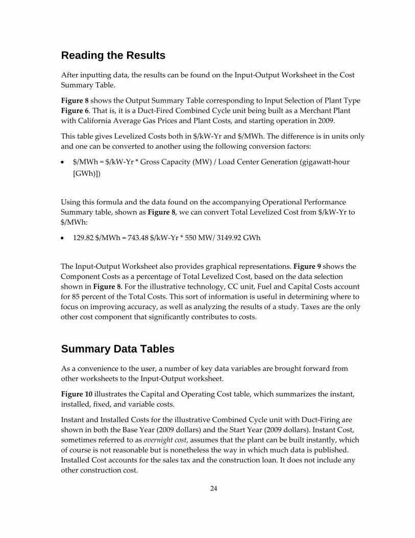
Reading the Results After inputting data, the results can be found on the Input‐Output Worksheet in the Cost Summary Table.

Figure 8 shows the Output Summary Table corresponding to Input Selection of Plant Type Figure 6. That is, it is a Duct‐Fired Combined Cycle unit being built as a Merchant Plant with California Average Gas Prices and Plant Costs, and starting operation in 2009.

This table gives Levelized Costs both in $/kW‐Yr and $/MWh. The difference is in units only and one can be converted to another using the following conversion factors:

• $/MWh = $/kW‐Yr * Gross Capacity (MW) / Load Center Generation (gigawatt‐hour [GWh)])

Using this formula and the data found on the accompanying Operational Performance Summary table, shown as Figure 8, we can convert Total Levelized Cost from $/kW‐Yr to $/MWh:

• 129.82 $/MWh = 743.48 $/kW‐Yr * 550 MW/ 3149.92 GWh

The Input‐Output Worksheet also provides graphical representations. Figure 9 shows the Component Costs as a percentage of Total Levelized Cost, based on the data selection shown in Figure 8. For the illustrative technology, CC unit, Fuel and Capital Costs account for 85 percent of the Total Costs. This sort of information is useful in determining where to focus on improving accuracy, as well as analyzing the results of a study. Taxes are the only other cost component that significantly contributes to costs.

Summary Data Tables As a convenience to the user, a number of key data variables are brought forward from other worksheets to the Input‐Output worksheet.

Figure 10 illustrates the Capital and Operating Cost table, which summarizes the instant, installed, fixed, and variable costs.

Instant and Installed Costs for the illustrative Combined Cycle unit with Duct‐Firing are shown in both the Base Year (2009 dollars) and the Start Year (2009 dollars). Instant Cost, sometimes referred to as overnight cost, assumes that the plant can be built instantly, which of course is not reasonable but is nonetheless the way in which much data is published. Installed Cost accounts for the sales tax and the construction loan. It does not include any other construction cost.

Figure 11 shows the effect of station service and transformer and transmission losses on the Capacity and Energy values.

Figure 12 summarizes operational performance factors. Figure 13 is the fuel cost summary.

Figure 8: Output Summary Table

Start Year = 2009 (2009 Dollars) $/kW-Yr $/MWhCapital & Financing - Construction $172.85 $30.26Insurance $8.35 $1.46Ad Valorem Costs $11.36 $1.99Fixed O&M $9.52 $1.67Corporate Taxes (w/Credits) $56.84 $9.95 Fixed Costs $258.91 $45.32Fuel & GHG Emissions Costs $418.13 $73.19Variable O&M $20.88 $3.66Variable Costs $439.01 $76.85Transmission Service Costs $29.74 $5.21Total Levelized Costs $727.66 $127.38

SUMMARY OF LEVELIZED COSTSCombined Cycle Standard - 2 Turbines, Duct Firing

OUTPUT RESULTS


25

Figure 9: Graphical Summary of Output Table

Capital & Financing ‐Construction

25%

Insurance1%

Ad Valorem Costs2%

Fixed O&M1%Corporate Taxes

(w/Credits)8%

Fuel & GHG Emissions Costs

60%

Variable O&M3%

Levelized Cost Components By Percentage


Figure 10: Key Capital and Operating Cost Summary

Capital & Operating Costs Base Yr Start Yr Levelized

2009 2009 2009 Instant Cost ( $/kW) $1,078 $1,078 N/A Installed Cost ( $/kW) $1,256 $1,256 N/A Fixed O&M Cost ( $/kW-Yr) $8.30 $8.30 $9.52 Variable O&M Cost ( $/MWh) $2.97 $2.97 $3.66


Figure 11: Capacity and Energy Summary

Capacity & Energy Summary Capacity Effective Energy 2009 (MW) (MW) (GWh)

Gross (Dependable) 550.0 550.0 3,321.5 Net Capacity - Plant Side 534.1 534.1 3,225.1 Net Capacity - Transmission Side 531.4 531.4 3,209.0 To Delivery Point 520.3 520.3 3,141.9


26

27

Figure 12: Summary of Operational Performance Factors

Operational Performance Factor Hours Scheduled Outage Factor 6.02% 527.4 Forced Outage Rate (FOR) 2.24% 140.5 Operational (Service) Hours Per Year 6,132.0 Equivalent Availability Factor 91.87% Capacity Factor 70.00%


Figure 13: Fuel Use Summary

Fuel Use Summary 2009 Levelized Average Heat Rate (Btu/kWh) 7,050 7,159 Fuel Use (MMBtu) 23,776,830 23,776,830 Fuel Price ($/MMBtu) $6.56 $9.67


Annual Cost Summary A special convenience of the COG Model is its upfront summary of annual costs. Although levelized cost is the most commonly used output of the COG Model, many studies rely on actual yearly costs. These costs are summarized in the Input‐Output Worksheet to promote (or make easier) these types of studies.

Figure 14 shows the actual annual costs that were used to calculate the present values and then the levelized costs, in both graphical and numerical format.

Figure 15 shows the corresponding Asset Rental Prices, which is not used otherwise in the COG Model. It is a sophisticated concept that is not commonly used, as explained in Attachment B.

The Input‐Output worksheet also has two ancillary functions: Screening Curves and Sensitivity Analysis Curves.

Figure 14: Annual Costs – Merchant Combined Cycle Plant

$0$20$40$60$80

$100$120$140$160$180$200

2009 2010 2011 2012 2013 2014 2015 2016 2017 2018 2019 2020 2021 2022 2023 2024 2025 2026 2027 2028

$/M

Wh

Year

Annual Fixed and Variable Power Plant Costs$/MWh

Total Costs

Variable CostsFixed Costs

Levelized NPV 2009 2010 2011 2012 2013 2014 2015 2016 2017 2018 2019 2020 2021 2022 2023 2024 2025 2026 2027 2028

Fixed Costs $45 $374 $42 $42 $43 $43 $44 $44 $45 $46 $46 $47 $47 $48 $49 $49 $50 $51 $51 $52 $53 $53Variable Costs $82 $677 $58 $61 $63 $68 $71 $75 $77 $82 $86 $92 $99 $102 $106 $113 $117 $122 $122 $127 $130 $133

Total Costs $127 $1,051 $99 $103 $106 $111 $115 $119 $122 $128 $132 $139 $146 $150 $154 $163 $167 $173 $173 $179 $183 $187 Source: Energy Commission

Figure 15: Annual Costs Based on Asset Rental Price


28

Using the Screening Curve Function Screening curves allow a user to view the levelized cost for various capacity factors, rather than the singular capacity factor that is typical of cost of generation models. This is useful in many ways. The most obvious is that it allows the user to estimate levelized costs for their specific assumption of capacity factor. It also allows the user to assess the cost risk of incorrectly estimating the capacity factor. It allows for the comparison of various technologies as a function of capacity factor – that is, at what capacity factor one technology becomes less costly than another.

The levelized costs of the screening curves can be shown as $/MWh or $/kW‐Yr. Figure 16 is an illustrative example of a $/MWh screening curve for advanced combustion turbine and a CC unit with duct firing. Figure 17 shows the corresponding interface window. This screening curve shows the advanced combustion turbine to be less expensive until a capacity factor equal to 65 percent—a surprising finding.

Figure 16: Screening Curve ($/MWh)

0

100

200

300

400

500

600

700

800

900

1,000

10% 20% 30% 40% 50% 60% 70% 80% 90% 100%

Levelized

Cost ($/M

Wh)

Capacity Factor

SCREENING CURVE — Start Year 2009 (Nominal 2009$)

Combustion Turbine ‐ 49.9 MWCombined Cycle Standard ‐ 2 Turbines, Duct FiringBiomass ‐ Co‐gasification IGCC (2018)Geothermal ‐ Binary

Solar ‐ Parabolic Trough

Solar ‐ Photovoltaic (Single Axis)


29

Figure 17: Interface Window for Screening Curve


30

Using the Sensitivity Curve Function Although the screening curves are useful, they address only one variable to the base case assumptions when estimating levelized costs – the capacity factor. Staff’s new sensitivity curves address a multitude of assumptions: capacity factor, fuel prices, installed cost, discount rate weighted average cost of capital (WACC), percent equity, cost of equity, cost of debt, and any other variable that should be considered. Sensitivity curves show the effect on total levelized cost by varying any of these parameters in three formats:

• Levelized cost ($/MWh or $/kW‐Yr)

• Change in levelized cost as a percentage

• Change in levelized cost as incremental levelized cost from the base value ($/MWh or $/kW‐Yr).

Figure 18 shows an illustrative example of a sensitivity curve. Figure 19 shows the interface window for the above sensitivity curve.

Figure 18: Sample Sensitivity Curve

0

20

40

60

80

100

120

140

160

180

-60% -50% -40% -30% -20% -10% 0% 10% 20% 30% 40% 50% 60% 70% 80% 90% 100%

Leve

lized

Cos

t ($/

MW

h)

Relative Change

Effect on Levelized Cost of Input Assumptions Combined Cycle Standard – 2 Turbines, No Duct Firing

Capacity FactorFuel PriceInstalled CostDiscount Rate (WACC)Percent EquityCost of EquityCost of DebtFixed O&MVariable O&MLoan TermBook Life


31

Figure 19: Interface Window for Sensitivity Curves


32

33

CHAPTER 4: Detailed Description of Worksheets This chapter provides detailed descriptions of the COG Model worksheets not provided elsewhere. This does not include every item in the model as some entities are either self evident or are defined in the Definitions Appendix (Appendix A).

Input-Output Worksheet The following are detailed descriptions of the terms used in the Input Selection Panel.

• Plant Type Assumptions—Using macros, this selection option collects data from the Plant Type Assumptions worksheet for the selected technology. All such selected data appears in the COG Model as shaded in turquoise. This version is more sophisticated than the 2007 version in that it provides high and low data in addition to the average data previously provided. To do this, there are three corresponding Plant Type Assumptions worksheets:

○ Plant Type Assumptions Mid‐range (PTA – Mid)

○ Plant Type Assumptions Hi‐range (PTA – Hi)

○ Plant Type Assumptions Lo‐range (PTA – Lo)

The Plant Type Assumptions worksheet selects the data from one of the above three PTA worksheets, depending on which Cost Scenario is selected in the Input Selection Table.

• Financial Assumptions—Using macros, this selection option collects data from the Financial Assumptions worksheet for the selected ownership. All such selected data appears in the COG Model as shaded in tan.

• Ownership type—This cell is largely an Excel© limitation and is ignored for most purposes.

• General Assumptions—Using macros, this selection option collects data from the General Assumptions worksheet for the selected ownership. All such selected data appears in the COG Model as shaded in light yellow. Generally, this will be “Default” until other scenarios are defined by the user.

• Base Year—This is reported data from the COG Model and is not selected by the user. It is the year that corresponds to the data in the Plant Type Assumptions worksheet. This data must then be escalated up to the in‐service year.

• Fuel Type—This is also reported data and is set based on the Plant Type Assumption selection.

34

• Data Source—This is informational as to the source and date of the data and also comes from the Plant Type Assumptions Worksheet.

• Start Date—This is entered by the user, not selected. It is the year the plant is to come on‐line and delivers power. It sets the beginning of the study period and the year for which the levelized costs are reported.

• Fuel Price Forecast—This affects the selection of gas‐fired units (SCs and CCs) only. It allows the COG Model to be run on utility‐specific gas prices. The Fuel Type option overrides all other fuel selections. Note: For gas‐fired units, this must be set after the General Assumptions selections, or it will be reset back to its original value.

• Study Perspective—This is the point where the levelized costs are calculated. If the power delivered is metered right at the plant, the user selects “At Busbar‐ Plant Side.” This is assumed to be the low side of the uplift transformer. This results in the transformer and transmission losses in the Data 1 worksheet being set to zero. If the user selects “At Busbar ‐ Transmission Side,“it is assumed to be the high side of the uplift transformer. This results in Transformer losses collected from the General Assumptions sheet and set into the Data 1 Worksheet. If the user selects “To Delivery Point,” then the transmission and transformer losses are collected from the General Assumptions Worksheet and are set into the Data 1 Worksheet. For this to work correctly, the General Assumptions option has to be selected after the Study Perspective option has been set.

• Reported Construction Cost Basis—Sets the Data 2 capital cost as either Instant or Installed, depending on how the data is entered. In 2007, gas‐fired units were entered as Installed Costs, and all others were entered as Instant Costs. In this version, all costs are entered as instant costs, but the option is still provided for the user to enter installed costs into the COG Model should this be desired

• Turbine Configuration—This is for CC units only. The baseline configuration in the COG Model is for two combustion turbine units with one steam turbine. This option allows the user to set the cost for other configurations. This number is to be set to the total number of combustion turbines regardless of the number of steam turbines.

• Carbon Price Forecast—Sets the price of carbon. Although this feature is in the model, the actual prices have not been determined by the Energy Commission. It is up to the user to define these costs if this feature is to be used.

• Cost Scenario—Sets the cost scenario as average, high, or low. This changes all technology and financing assumptions.

• Tax Loss Treatment—Sets the assumption on whether the tax benefits are to be realized in a single year or are assumed to have a minimum tax set at zero with tax losses carried forward.

35

The following are definitions for the terms used in the Output Summary Table, which provides the desired levelized costs. The levelized costs are collected from the Income Statement (Cells D47–D53).

• Capital and Financing Costs—The capital cost is the total cost of construction, including land purchase, land development, permitting, interconnection, environmental control equipment, and component costs. The financing costs are those incurred through debt and equity financing and are incurred by the developer annually, similar in structure to financing a home. These annual costs, therefore, are essentially levelized by this cost structure.

• Insurance Cost—This is the cost of insuring the power plant, similar to the insuring of a home. For a Merchant/POU the first year cost is estimated as a percentage of the installed cost per kW and then escalated by forward inflation throughout the book life (period of the calculations). For an IOU plant, the annual cost is a percentage of the book value/rate base, and the subsequent yearly cost decreases over time.

• Ad Valorem Cost—The cost of annual property tax payments that are paid as a percentage of the assessed value and usually transferred to local governments. POU power plants are generally exempt from these taxes but may pay in‐lieu fees. The assessed values for power plants are set by the State Board of Equalization (BOE) as a percentage of book value for an IOU and as depreciation‐factored value for a merchant facility.

• Fixed O&M Costs—These are the costs that occur regardless of how much the plant operates. These are not uniformly defined by all interested parties but generally include staffing, overhead and equipment (including leasing), regulatory filings, and other direct costs.

• Corporate Taxes—These are state and federal taxes, which are not applicable to a POU. The federal taxes are adjusted for the state taxes similar to adjustment rates for a homeowner.

• Fuel Cost—The cost of fuel used by the power plant is most commonly expressed in $/MWh. For a thermal power plant, it is the heat rate (British thermal unit per kilowatt‐hour (Btu/kWh)] multiplied by the cost of the fuel ($/MMBtu). This includes start‐up fuel costs as well as the on‐line operating fuel usage. Allowance is made for the degradation of the heat rate over time.

• Variable O&M—These costs are a function of the hours of operation of the power plant. Most importantly, this includes yearly maintenance and overhauls. Variable O&M also includes repairs for forced outages, consumables, water supply, and annual environmental costs.

The Input‐Output Worksheet also displays annual (unlevelized) costs, which are shown above in Figure 14.

36

The Input‐Output worksheet has three additional functions:

• Save scenarios

• Screening curves

• Sensitivity analysis curves

These are described in the previous chapter.

Data 1 Worksheet This worksheet holds key data that the macro collects from the Assumptions worksheets, as well as performing some minor calculations. The data categories are:

• Plant Capacity & Energy Data—Capacity, Energy & Losses

• Operational Performance Data—Percent Output, Percent of Year Operational, Outage, Capacity & Availability Factors

• Fuel Use Data—Heat Rates and Degradation Factors and Startup Fuel Use

• Financial Information—Capital Structure, Inflation Factors, Life & Taxes

• Tax Information—Tax Rates

• Alternative Techs Tax Benefits

○ Business Energy Tax Credit (BETC)

○ Renewable Energy Production Tax Credit (REPTC)

○ Geothermal Depreciation Allowance (GDA)

○ Renewable Energy Production Incentive ( REPI)

Plant Capacity and Energy Data Figure 20 shows the Plant Capacity and Energy table for the CC with duct‐firing technology. All but the last item captures the capacity and energy at three levels:

• Gross Capacity—Capacity at the generation level.

• Net Capacity‐Plant Side—Capacity at the power plant busbar, allowing for station service. This is at the low side of the uplift transformer.

• Net Capacity‐Transmission Side—Capacity at the transmission busbar, which is the high side of the uplift transformer.

• Load Center Capacity—Capacity at the point of delivery, allowing for transformer and transmission losses.

Figure 20: Plant Capacity and Energy Data

Plant Capacity & Energy DataEffective Capacity

(MW)

Average Annual Energy (GWh)

Gross Capacity (MW) 550.00 550.00 3329.89Plant Losses 2.90%Net Capacity (MW) - Plant Side 534.05 534.05 3233.33Transformer Losses 0.50%Net Capacity (MW) - Transmission Side 531.38 531.38 3217.16Transmission Losses 2.09%Delivered Capacity (MW) 520.3 520.27 3149.92Annual Capacity Degradation Rate 0.20%STUDY PERSPECTIVE 520.27 520.27 3149.92 Source: Energy Commission

Treatment of Losses The above differences in capacity are due to losses. Since the treatment of losses is a bit subtle, it is explained in detail herein. The COG Model has three categories of losses:

• Plant Losses (Parasitic Losses)—Losses due to on‐site power uses.

• Transformer Losses—Losses in the uplift transformer, between the plant bus bar (low side of the transformer) and the transmission busbar (high side of the transformer).

• Transmission Losses—Losses between the transformer and the Delivery Point.

The site load losses vary depending on the technology. The COG Model allows for different site losses for each cost basis. Losses for the gas‐fired units were estimated by Aspen and losses for the other units were estimated by KEMA Consulting Firm. For the staff’s illustrative CC unit, the average losses are estimated as 2.9 percent. Thus the 550 MW is reduced to 534.05 MW (550 [100%‐2.9%]).

Transformer Losses are the losses in uplifting the power from the low voltage side of the transformer (Generator Voltage) to the high voltage side of the transformer (Transmission Voltage). For staff’s illustrative CC unit, this is estimated using the CPUC Market Price Referent (MPR) value of 0.5 percent, which was reconfirmed as reasonable. Transmission Losses represent the power lost in getting the power from the high side of the Transformer to the Delivery Point. For staff’s illustrative CC unit, this value is estimated as 2.09 percent.

37

38

Annual Capacity Degradation Rate This value captures the degradation of capacity averaged over the life of the power plant. It accounts for both the degradation of capacity due to wear and tear and the increases in capacity due to periodic overhauls. It is an average as the plant capacity degrades and then partially restored due to the many overhauls the plant experiences during its lifetime. Capacity Degradation is provided as an annual percentage and is located in Cell C26 of the Data 1 Worksheet and is brought forward from the Plant Type Assumptions Worksheet, Row 9.

The implementation of the capacity degradation factor is done by making two simplifying assumptions. The first assumption is that the capacity degradation can be ignored in the calculation of $/kW‐Yr of the Income Statement Worksheet, based on the assumption that the $/kW‐Yr should be considered to be based on the original installed gross capacity, similar to installed cost. That is, it should not be based on the average value of the degraded capacity (for example, the geometric mean of time‐weighted capacities over the study period). The effect of capacity degradation is captured only on the energy side.

The second assumption is that the impact on the energy generated can be represented by a constant annual average value, rather than as actual annual values that decrease over the years. The implementation of this capacity degradation is captured in the average energy values of Cells 19, 21, 23, and 25 (Data 1 Worksheet), using the following Excel formulas, where PMT is the annual payment, which is the levelized cost.

Average Annual Energy for Gross Capacity—PMT(rate,nper,pv)

○ rate(Interest Rate) = Discount Rate

○ nper(number of periods) = Book Life

○ pv(Present Value) = PV((1+DiscountRate)/ (1‐AnnCapDegredationRate)‐1, BookLife, OpHrsPerYr*GrossMW/1000* AverageOutputPct))

Average Annual Energy for Net Capacity—Plant Side: PMT(rate,nper,pv)

○ rate (interest rate) = Discount Rate

○ nper(number of periods) = Book Life

○ pv(Present Value) = PV((1+DiscountRate)/(1‐AnnCapDegredationRate)‐1,BookLife,OpHrsPerYr*OpCapMW/1000))

Average Annual Energy for Net Capacity—Transmission Side: PMT(rate,nper,pv)

○ rate (interest rate) = DiscountRate

○ nper(number of periods) = BookLife

○ pv(Present Value) = PV((1+DiscountRate)/(1‐AnnCapDegredationRate)‐1,BookLife,OpHrsPerYr*OpCapMW*TransformerLosses/1000))

Average Annual Energy at Load Center—PMT(rate,nper,pv)

○ rate (interest rate) = DiscountRate

○ nper(number of periods) = BookLife

○ pv(Present Value) = PV((1+DiscountRate)/(1‐AnnCapDegredationRate)‐1,BookLife,OpHrsPerYr*EffectiveMW/1000))

In each of the above cases, an average energy value, PMT, is calculated by first calculating a present value (PV) of the actual energy values and then using that PV to find the levelized energy value, PMT, similar to what is done in the Income Statement Worksheet for dollar values. This calculation of the PV is subtle and can best be illustrated using simplified nomenclature. If Et are the annual decreasing energy values for years (t), 0 through N, then Et=EC(1‐CD)t, where EC is the annual energy in the absence of capacity degradation and CD is the Capacity Degradation Factor. Each of the annual degraded values of this energy series can be converted to a present value by dividing by the factor (1+DR)t, where DR is the discount rate and t is number of the year. The present value (PV) of the entire series, therefore, can be represented as:

∑∑== +

−=

+=

N

tt

tC

N

1tt

t

DR)(1CD)(1E

DR)(1EPV

This can be easily rearranged to:

∑∑== −+

=−+

=N

1tt

CN

ttt

C

CD)]DR)/(1[(1E

CD)/(1DR)(1EPV

Adding 1 and subtracting 1 in the denominator, as shown, does not change the value but allows the user to put this in a more usable form:

1CD)]DR)/(1[(1i:where;i)(1

E1]CD)DR)/(1(1[1

EPVN

1tt

CN

1tt

C −−+=+

=−−++

= ∑∑==

The formula is now a present value of constant value EC, where the interest rate is equal to

1CD)]DR)/(1[(1 −−+ .

The implementation of this into Excel can be illustrated for the above Gross MW energy case:

pv=(rate,nper,pmt)

39

○ rate= 1CD)]DR)/(1[(1i −−+= =[(1+DiscountRate)/(1‐AnnCapDegradation Rate)]‐1

○ nper=BookLife

○ pmt= EC= OpHrsPerYr*GrossMW/1000* AverageOutputPct))

Average Annual Energy for Gross Capacity—PMT(rate,nper,pv)

○ rate(Interest Rate) = DiscountRate

○ nper(number of periods) =,BookLife,

○ pv(Present Value) = PV((1+DiscountRate)/ (1‐AnnCapDegredationRate)‐1, BookLife, OpHrsPerYr*GrossMW/1000* AverageOutputPct))

The final division by “(1‐AnnCapDegradation)” is for aligning the yearly values of the degradation factor with those of the discount rate.

Operational and Performance Data Figure 21 shows the Operational and Performance Data table for the CC with duct‐firing technology.

Average Percent Output This factor is used for generating technologies, such as solar and wind, which have variable outputs. This factor estimates the average MWs for these units. For example, Solar Photo Voltaic may have the potential to achieve 50 MW but will typically be below that value so that it has an average of 12.5 MW over the year. Accordingly, the Average Percent Output is 25 percent (12.5/50= 0.25 = 25%).

Planned Percent of Year Operational This factor is used to capture the effect of economic dispatch. It is used to adjust the capacity factor for any unit that will have its operational hours limited due to economic dispatch—primarily used for the conventional generating units. Its function can be illustrated for a combustion turbine, which is typically expected to operate only 5 percent of the year, so that its Planned Percent of Year Operational Factor is 5 percent. Actually, this is simplistic as the Capacity Factor also depends on the Forced Outage and Schedule Outage Factor. For a combined cycle unit, the Planned Percentage of Year Operational Factor is set at 71.6 percent to achieve the known average capacity factor for a combined cycle unit of 70 percent.

40

Figure 21: Operational and Performance Data

Operational Performance Data Hours/YrAverage Percent Output 100.00%Planned Percent of Year Operational 71.6% 6,273Number Of Annual Starts 25Scheduled Outage HoursOR Scheduled Outage Factor 6.02%Modeled Scheduled Outage Factor 6.0% 527Final Planned Operational Hours 6,273Forced Outage Rate (FOR) 2.24% 141Operational (Service) Hours Per Year 6,132Total Operating Hours Over Life Of Plant 122,640Equivalent Availability Factor 91.87%Net Capacity Factor (NCF) 70.00%


Scheduled Outage Hours and Factor Scheduled Outage Hours (SOH) are those hours when the power plant is on scheduled maintenance. This includes not only annual maintenance but also forced outages that can be delayed beyond the next weekend, called “Maintenance Outages.” These are North American Reliability Council (NERC) definitions that are created by its Generating Availability Data Service (GADS) unit. These definitions are more carefully explained in the Definitions section at the end of this User’s Guide. These outages calculated as a percentage of the total year are called Scheduled Outage Factor (SOF). In the COG Model, SOF = SOH / 8,760 hours.

Forced Outage Hours and Rate The Forced Outage Hours (FOH) and Forced Outage Rate (FOR) are a measure of the power plant’s reliability. FOH are those hours when a power plant is forced out of operation due to equipment failure. FOR is the ratio of the FOH to those hours when the plant attempts to be operational. Hours when the plant is not called on to operate are not applicable to the calculation. Accordingly, FOR = FOH/(FOH+SH), where SH is the Service Hours. For purposes of simplification, these terms are used in the COG Model, but they are not strictly accurate in that there are partial outages where the plant is able to operate at partial power. To capture this subtlety, Equivalent FOH and FOR should be entered into the model. FOR becomes EFOR and the formula becomes progressively more complicated, but in its simplest form, it is EFOR = (FOH+EFDH) / (FOH+SH+EFDHRS). The exact formula has been further complicated by recent NERC/GADS definitions. To get the exact formula and complete understanding, one needs to go to the Definitions section.

41

Equivalent Availability Factor This indicates the Availability of the Power Plant as the percentage of the year that the plant is not on maintenance and not forced out. This factor represents when the plant is available, not when it is running, which is characterized by the capacity factor described below. Availability Factor (AF) is calculated as AF = (1‐FOR)* (1‐SOF). One must remember, however, that FOR is really EFOR and SOF is really ESOF. For this more exact case, AF becomes Equivalent Availability Factor (EAF). As before, it is necessary to go to the Definitions section for a complete understanding.

Net Capacity Factor The Net Capacity Factor (NCF) is a measure of how much the plant is used. In simplest terms, it is equal to the ratio of the energy generated by the power plant to the energy that could be generated if it operated at full power for the entire year. The word “Net” signifies that the net capacity is used. The exact formula that the COG Model uses is: Net Capacity Factor (NCF) = (Operational Hrs/Yr*Effective Operating Capacity [MW]) / ([8760*Net Capacity [MW]).

Fuel Use Data Figure 22 shows the Fuel Use Data table for the CC with duct‐firing technology.

Figure 22: Fuel Use Table

Efficiency

Annual Average Heat Rate (HHV) Adjusted for Capacity Factor 7,050 Btu/kWh 48.4% Adjusted Net Of Startup 7,039 Btu/kWh 48.5%

Annual Heat Rate Degradation 0.20%Fuel Consumption/Hour 3,871 MMBtu/HrStart Up Fuel Use 1,540 MMBtu/StartAverage Annual Fuel Use 23,776,830 MMBtu

Fuel Use


There are two average annual heat rates.

• Adjusted for capacity factor

• Adjusted for startup energy

Adjusted for Capacity Factor Base Year Heat Rates are provided in the Plant Type Assumptions Worksheet and are forwarded to the Data 1 worksheet by the macros. Only the CC heat rates are adjusted for

42

43

capacity factor in the COG Model. The base year heat rate is calculated in the Plant Type Assumptions Worksheet using a regression of the Energy Commission’s QFER data. This regression is shown in a worksheet of the COG Model, called, “CC_Heat Rate” as a function of CF. The default CC unit with duct‐firing has a capacity factor of 70 percent. This value is varied for the screening curve function.

Adjusted for Startups This is the estimated heat rate without the energy used in startups and as such is a better heat rate. This is estimated by assuming the annual number of startup and the fuel used in each startup and increasing the heat rate accordingly. The estimate has no effect on the actual average heat rate as it is calculated based on QFER data, which inherently captures all fuel usages including startup fuel. The heat rate net of startups is calculated by backing out the estimated startup fuel usage.

Heat Rate Degradation The heat rate degradation for the units other than the CC and SC was provided by NCI consulting company. The somewhat limited documentation for this is provided in the 2009 IEPR Cost of Generation Report. The heat rate degradation for the gas‐fired units is as follows:

• For Simple Cycle Units: 0.05 percent per year

• For Combined Cycle Units 0.2 percent per year

These degradation estimates are based on a December 7, 2005, e‐mail from James Shoonmaker to Will Walters, which incorporates a General Electric Technical Bulletin GER‐3567H, Last update 2000, which are included as Attachment A.

General Electric’s rule is that SC units degrade 3 percent every 24,000 hours, at which time they receive an overhaul and return to 1 percent degradation—that is, they recover two‐thirds of the degradation. Assuming that they operate at an average of 5 percent capacity factor, an overhaul will not be necessary for 55 years, which is beyond the book life (24,000 hrs/(8760*0.05hrs/yr=54.8 yrs). This is equivalent to 0.05 percent degradation per year (3% / 55 years = 0.05%). This is illustrated in Figure 23.

The computation for the CC units is more complex due to its higher capacity factor—estimated to be roughly 70 percent for duct‐fired and 75 percent for non‐duct‐fired, based on the QFER data and other historical information. The 70 percent capacity factor calls for an overhaul every 3.9 years and the non‐duct‐fired unit every 3.6 years. Approximating both of these as 4 years results in four major overhauls during its 20‐year book life, as shown in Figure 24. Since the steam generator portion remains essentially stable, the overall system deteriorates 2.4 percent during the four‐year period and recovers two‐thirds of its deterioration during the overhaul. Each subsequent end of degradation point and recovery point is 0.667 percent higher than the last. This gives an end point at 20 years of 4.67 percent.

The equivalent degradation of 0.24 percent can be calculated as the slope of the line that has the equivalent area under the curve, 0.24 percent per year (4.67%/20 = 0.24%).

These approximations are quite adequate as the effect on levelized cost is quite small; in fact, the elimination of this factor has a small effect: 0.5 percent for simple cycle units and 0.9 percent for CC units.

Figure 23: Heat Rate Degradation—Simple Cycle

EQ UIVALENT HEAT RAT E DEG RADAT IO N O F SIM PLE CYCLE UNIT @ 5% CF

0.0%

0.5%

1.0%

1.5%

2.0%

2.5%

3.0%

3.5%

4.0%

0 2 4 6 8 10 12 14 16 18 20

Years of Operation

Deg

rad

atio

n

Equivalent SC Degradation


44

Figure 24: Heat Rate Degradation – Combined Cycle

0.0%

0.5%

1.0%

1.5%

2.0%

2.5%

3.0%

3.5%

4.0%

4.5%

5.0%

0 4 8 12 16

Hea

t Rat

e D

egra

datio

n

Years of Operation20

Actual Degradation

Equivalent Degradation


Financial Information Figure 25 shows the Financial Information table for the CC with duct‐firing with merchant financing.

Equity The value shown as 60 percent is the percentage of capital raised that is financed through stock investments. The value shown as 14.47 percent is the interest paid to the investors.

Debt The value shown as 40 percent is the percentage of capital raised that is financed through bank loans, and the value shown as 7.49 percent is the average interest paid on the loan.

Discount Rate The value shown as 10.46 percent is the discount rate and is assumed to be equal to the weighted average cost of capital (WACC). The WACC is adjusted for tax reduction in federal taxes for state taxes and is calculated as:

WACC =Capital Structure Equity %* Cost of Capital Equity % + Capital Structure Debt Financed % * Cost of Capital Debt Financed %* (1‐ Total Tax Rate)

Real Discount Rate The value shown as 8.76 percent is the real discount rate, which is used in the overhaul calculation that is described in detail in the section on the Overhaul Worksheet.

45

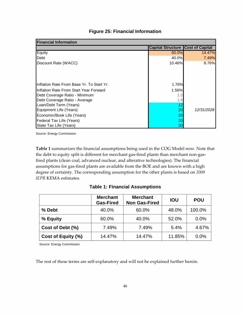
Figure 25: Financial Information

Capital Structure Cost of CapitalEquity 60.0% 14.47%Debt 40.0% 7.49%Discount Rate (WACC) 10.46% 8.76%

Inflation Rate From Base Yr. To Start Yr. 1.76%Inflation Rate From Start Year Forward 1.56%Debt Coverage Ratio - Minimum 1.5Debt Coverage Ratio - Average 1.8Loan/Debt Term (Years) 12Equipment Life (Years): 20 12/31/2028Economic/Book Life (Years) 20Federal Tax Life (Years) 20State Tax Life (Years) 20

Financial Information


Table 1 summarizes the financial assumptions being used in the COG Model now. Note that the debt to equity split is different for merchant gas‐fired plants than merchant non‐gas‐fired plants (clean coal, advanced nuclear, and alterative technologies). The financial assumptions for gas‐fired plants are available from the BOE and are known with a high degree of certainty. The corresponding assumption for the other plants is based on 2009 IEPR KEMA estimates.

Table 1: Financial Assumptions

Merchant Gas-Fired

Merchant Non Gas-Fired IOU POU

% Debt 40.0% 60.0% 48.0% 100.0%

% Equity 60.0% 40.0% 52.0% 0.0%

Cost of Debt (%) 7.49% 7.49% 5.4% 4.67%

Cost of Equity (%) 14.47% 14.47% 11.85% 0.0% Source: Energy Commission

The rest of these terms are self‐explanatory and will not be explained further herein.

46

Tax Information Figure 26 shows the tax information. State and federal taxes are common to merchant and IOU power plants but not to POU plants, which are exempt from both taxes. Ad Valorem taxes are complex in that they are calculated differently for all the three developers. Merchant plants pay the shown rate based on installed cost, but IOU plants pay the shown rate based on its rate base value, which depreciates over the lifetime of the power plant. POU power plants are not required to pay Ad Valorem but generally make gratuitous “in‐lieu” payments.

Figure 26: Tax Information

Tax InformationFederal Tax = 35.0%CA State Tax = 8.84%Total Tax Rate = 40.7%CA Avg. Ad Valorem Tax = 1.10%Municipal in-lieu payment of property taxes YCA Sales Tax = 7.94%


Renewable Tax Benefits Information Figure 27 is the Renewable Tax Benefits table. It works in conjunction with the Financial Worksheet to define deductions and tax credits in the Income Statement Worksheet.

47

Figure 27: Tax Benefits

Tax & Production IncentivesEligible For BEITC Y ITC ExpirationEligible For Geothermal Depletion Allowance NEligible For REPTC Y PTC ExpirationEligible For REPI N REPI Expiration

Business Energy Investment Tax Credit (ITC) N BETC Limit ($) BETC Depreciation Adjustment BETC Limit (% Of Remaining Taxes) 100% BETC Calculation $0Geothermal Depletion Allowance N Percentage Depletion Limit (% Of Remaining Taxes)Renewable Energy Production Tax Credit (REPTC) N Duration REPTC Base Year REPTC In Start Year $/kWh 0.000REPI Tier REPI Tier I Proportion Paid 19% REPI Tier II Proportion Paid 18% REPI Duration REPI Base Year REPI In Start Year $/kWh 0.000California Property Tax Solar CreditCalifornia Solar Initiative $/kWh CSI Duration (years) Solar installed capacity forecast at time of construction 50 MWCalifornia Self-Generation Incentive Program /kW


Data 2 Worksheet The Data 2 Worksheet summarizes the Construction, Operation, and Maintenance Costs. In addition, it provides some factors for calculating the fixed and variable costs in the Income Statement Worksheet.

Construction Costs Figure 28 shows the Instant Capital Cost panel for a CC unit with duct‐firing. All costs are given in base year dollars. For the CC and simple cycle units, this is year 2005.

48

49

Note that there six categories of costs:

• Component Costs—Generator, boilers, pipeline and control system costs

• Land Costs—Acquisition and preparation cost

• Development Costs—Predevelopment, insurance and commitment fee

• Permitting Costs—Building, environmental and emission reduction credits (ERC) costs

• Interconnection Costs—Transmission, fuel/water/sewer costs

• Environmental Control Costs—Air emission controls and water treatment and cooling controls costs

The cell above the bottom line in this panel (shaded in turquoise) allows the user to insert a single value for the instant (or installed) cost and not provide the above detailed components of the cost.

Figure 29 is the panel that converts instant cost to installed cost. Each line is in nominal dollars for the year shown and represents the dollars expended in that year. The final value (in red) is in start year nominal dollars—in this case, 2009 dollars. The allowance for funds during construction (AFUDC) rate is assumed to be equal to the WACC.

Figure 28: Instant Costs

Instant Capital Costs ($)Financial Transaction Costs 0.0%Component CostTotal Overnight Cost $561,550,000

$0

Total Component Cost $561,550,000

Land Costs Acreage/MW Acreage/Plant 25.00 Additional Occupied Acreage Total Acres 25 Cost Per Acre Acquisition Cost $0 Land Prep Costs/Acre Total Land Prep Costs $0Total Land Costs $0Development Costs Predevelopment Expenses Construction Insurance & Installation

Commitment Fee

Total Development Costs $0Permitting Costs Local Building Permits Environmental Permits $5,500,000 Emission Reduction Credits Costs $25,835,397Total Permitting Costs $31,335,397Interconnection Costs (Linears) All connection costs $34,100,000 Transmission interconnection Fuel / water / sewer costsTotal Interconnection Costs $34,100,000Air Emission Controls Installation Costs $0Total Air Emission Controls Costs $0Water Treatment & Cooling Controls Installation Costs $0Total Water Treatment & Cooling Controls Costs $0Total Environmental Controls Costs $0Total Component Cost $561,550,000INPUT OVERRIDE CAPITAL COST - InstantDEFAULT TOTAL CAPITAL COST - Instant $626,985,397


50

Figure 29: Converting Instant to Installed Cost

Capital Construction Costs by Year (Nominal $)Escalation in Capital Costs 0.00%AFUDC Rate 10.46%

Cost %/Year Months inConstruction

Year2004 (-5) 0% $0 02005 (-4) 0% $0 02006 (-3) 0% $0 02007 (-2) 0% $0 02008 (-1) 25% $164,941,642 122009 (0) 75% $677,014,118 12

Cumulative Construction Costs by Year

Year


Figure 30 converts the instant and installed costs in total dollars to instant and installed cost in $/kW. The turquoise block, Input Override, allows the user to override all the calculations in Figure 28 and Figure 29 and enter the installed cost in start year dollars directly.

Figure 30: Converting Instant to Installed Cost

INPUT OVERRIDEInstalled Cost (2009 Dollars)Instant Cost (2009 Dollars) $1,140 Ratio of Installed Cost (2009 Dollars) $1,329 Installed toInstant Cost (2009 Dollars) $1,140 InstantInstalled Cost (2009 Dollars) $1,329 1.16553

Capital Costs (Nominal $/kW)


Both the Instant and Installed Costs ($/kW) are calculated in both Base Year and Start Year Dollars. First, the sum of these Instant Capital Costs is calculated in Base Year Dollars ($), then converted to Instant Costs ($/kW) by dividing by the Gross MW. These Base Year Costs can then be inflated to Start Year Costs, using the Deflator Series of the Inflation Worksheet. Both of these Instant Costs can then be converted to Installed Costs ($/kW) by allowing for Construction Costs. The Construction Costs are based on an estimated period of Construction, using the Cost of Capital for a Construction Loan, which is assumed to be equal to the AFUDC.

Operation and Maintenance Cost These costs are divided into two categories:

51

• Fixed O&M—Employee salaries, overhead, and equipment (including leasing), regulatory filings and other direct costs, as shown in Figure 31

• Variable O&M—Total Annual Maintenance, Water Supply, Plant Scheduling and Total Environmental Costs, as shown in Figure 32

Figure 31: Fixed O&M Cost

Employees FTE Hours/Year WagesManagers (Salary, $/Year)) 2.7 $164,282Plant Operators (Wage, $/Hour) 14.3 2,080 $34.95Mechanics (Wage, $/Hour) 2.9 2,080 $37.86Laborers (Wage, $/Hour) 0.5 2,080 $29.28Support Staff (Wage, $/Hour) 3.7 2,080 $26.91Total W-2 Wages, adjusted to Base Year $2,132,275Overhead Multiplier 1.593Annual Salary W/ Overhead ($) $3,395,782Annual Salary W/ Overhead ($/kW-Yr) $6.174150Non-labor Fixed O&M including ODC $/kW/Yr $2.13

INPUT OVERRIDEFixed O&M ($/kW-Yr) <-- Overrides above values.Total Fixed O&M ($/kW-Yr) $8.30

FIXED O&M COSTS


For the gas‐fired power plants, the employee salaries are calculated within the Plant Type Assumptions worksheet and have also been benchmarked against the values from the data survey. The non‐labor amount is calculated as an average value from the survey. For all other technologies, the fixed O&M is given as a total value that includes both the labor and non‐labor amounts.

Water Supply Costs Calculated as a function of the region. The cost per acre‐foot is taken from the Plant Site Air and Water Data Worksheet. The total cost of water is then calculated as cost per acre‐foot times the acre‐foot consumption, which is taken from the Technology Assumptions Worksheet, via a macro.

Plant Scheduling Costs The costs associated with coordinating plant bids and operational schedules with power marketers and transmission network access costs with the California ISO. These include transmission access fees, wheeling charges, and scheduler costs. These costs may be a share of costs spread across a portfolio of plants owned and managed by a single entity.

52

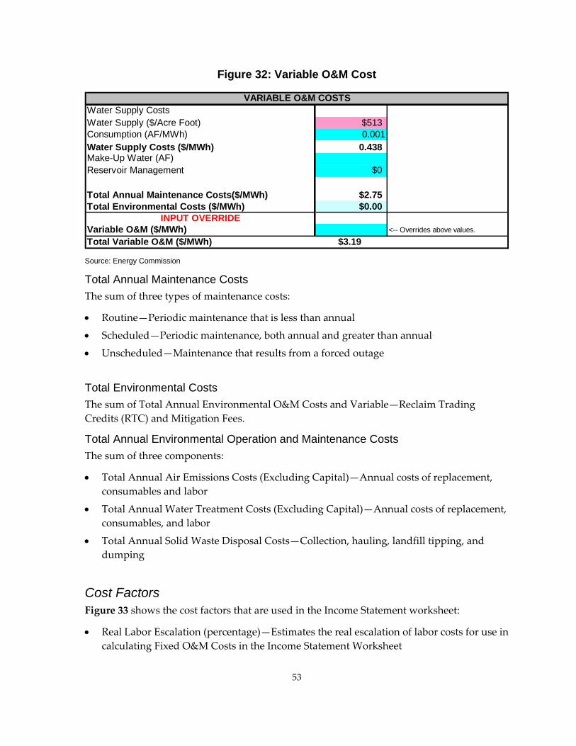
Figure 32: Variable O&M Cost

Water Supply CostsWater Supply ($/Acre Foot) $513Consumption (AF/MWh) 0.001Water Supply Costs ($/MWh) 0.438Make-Up Water (AF)Reservoir Management $0

Total Annual Maintenance Costs($/MWh) $2.75Total Environmental Costs ($/MWh) $0.00

INPUT OVERRIDEVariable O&M ($/MWh) <-- Overrides above values.

Total Variable O&M ($/MWh) $3.19

VARIABLE O&M COSTS


Total Annual Maintenance Costs The sum of three types of maintenance costs:

• Routine—Periodic maintenance that is less than annual

• Scheduled—Periodic maintenance, both annual and greater than annual

• Unscheduled—Maintenance that results from a forced outage

Total Environmental Costs The sum of Total Annual Environmental O&M Costs and Variable—Reclaim Trading Credits (RTC) and Mitigation Fees.

Total Annual Environmental Operation and Maintenance Costs The sum of three components:

• Total Annual Air Emissions Costs (Excluding Capital)—Annual costs of replacement, consumables and labor

• Total Annual Water Treatment Costs (Excluding Capital)—Annual costs of replacement, consumables, and labor

• Total Annual Solid Waste Disposal Costs—Collection, hauling, landfill tipping, and dumping

Cost Factors Figure 33 shows the cost factors that are used in the Income Statement worksheet:

• Real Labor Escalation (percentage)—Estimates the real escalation of labor costs for use in calculating Fixed O&M Costs in the Income Statement Worksheet

53

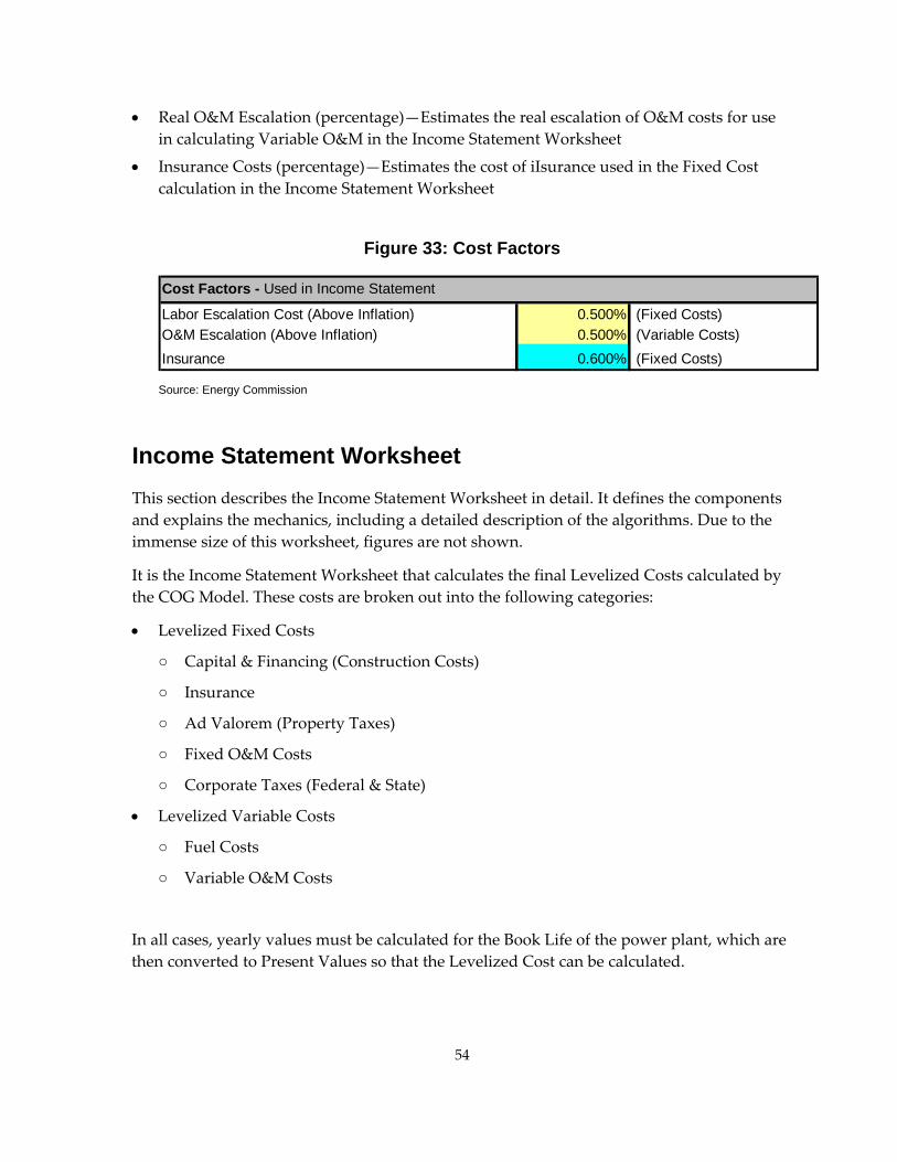
• Real O&M Escalation (percentage)—Estimates the real escalation of O&M costs for use in calculating Variable O&M in the Income Statement Worksheet

• Insurance Costs (percentage)—Estimates the cost of iIsurance used in the Fixed Cost calculation in the Income Statement Worksheet

Figure 33: Cost Factors

Cost Factors - Used in Income Statement

Labor Escalation Cost (Above Inflation) 0.500% (Fixed Costs)O&M Escalation (Above Inflation) 0.500% (Variable Costs)Insurance 0.600% (Fixed Costs)


Income Statement Worksheet This section describes the Income Statement Worksheet in detail. It defines the components and explains the mechanics, including a detailed description of the algorithms. Due to the immense size of this worksheet, figures are not shown.

It is the Income Statement Worksheet that calculates the final Levelized Costs calculated by the COG Model. These costs are broken out into the following categories:

• Levelized Fixed Costs

○ Capital & Financing (Construction Costs)

○ Insurance

○ Ad Valorem (Property Taxes)

○ Fixed O&M Costs

○ Corporate Taxes (Federal & State)

• Levelized Variable Costs

○ Fuel Costs

○ Variable O&M Costs

In all cases, yearly values must be calculated for the Book Life of the power plant, which are then converted to Present Values so that the Levelized Cost can be calculated.

54

55

Levelized Fixed Costs

Capital and Financing Capital and Financing covers the capital cost of the equipment and facilities plus the cost of constructing and financing the power plant. The capital cost is calculated in the Data 2 worksheet, first as instant cost, which covers the cost of the equipment and all related facilities including licensing, and then as installed cost, which covers the construction costs. These costs are calculated both in the base year and the in‐service year as $/kW and are used in the Income Statement Worksheet to calculate the financing costs (debt and equity).

Insurance Insurance is calculated using a percentage rate that is presently set at 0.6 percent. This percentage rate is designated as “InsurancePct” and comes from the Data 1 Worksheet, which in turn gets its data from the Plant Type Assumptions Worksheet.

For an IOU, the percentage rate is applied against the book value, and since the book value decreases over the life of the calculation, the insurance payments are higher in the early years and lower in the later years.

For a Merchant and Municipal Plant, the percentage rate is applied against the Installed Cost per kilowatt. The Installed Cost per kilowatt is calculated on the Data 2 Worksheet as a Base Year value. This product is then escalated first to the Start Year using Historical Inflation and then throughout the Book Life of the project using the Forward Inflation.

Ad Valorem Ad Valorem, which is the traditional name for property taxes, is calculated differently for municipal, IOU and merchant plants. For a Municipal Plant the property taxes are zero by definition. For an IOU, it is calculated as the Ad Valorem Tax Rate (Data 1) times the Rate Base. For a merchant plant it is calculated as a Percentage Rate (Data 1) times the Installed Cost per Kilowatt. Also for merchant‐owned plants Installed cost is escalated at the Prop 13 limit =2 percent.

Fixed Operation and Maintenance The Base Year value is calculated in the Data 2 Worksheet, which relies on data in the Overhaul and Plant Site Air and Water Data Worksheets. The yearly values are then escalated to the start year using the Historical Inflation and then throughout the Book Life using the Forward Inflation Rate. Both use the same Nominal Inflation, but each has its own Real Escalation Factor: Fixed O&M uses Labor Escalation Rate whereas Variable O&M uses O&M Escalation Rate.

Corporate Taxes Corporate Taxes are state and federal taxes. They are individually but similarly calculated as a Tax Rate (Data 1 Worksheet) times the quantity Before Tax Income (Operating Income) minus Deductions, this quantity must then be reduced by the Tax Credits—similar to

56

personal taxes. The deductions for state are interest on the loan and depreciation. It is the same for the federal taxes except that there is also the standard deduction for state taxes (so that state taxes are not paid twice, similar to personal taxes). In addition, there are special deductions for fossil fuel technologies, such as Tax Deduction for Manufacturing Activities (TDMA), and some alternative technologies, such as Geothermal Depletion Allowance (GDA). There are also tax credits available, such as Business Expense Tax Credit (BETC), Renewable Energy Production Tax Credit (REPTC), and Renewable Energy Production Incentive (REPI). Conceptually this seems straight forward but is complicated by the subtleties in the calculation of the Operating Income as explained below.

Levelized Variable Costs

Fuel Cost Fuel Cost is calculated only for fossil‐fueled generators, nuclear, gasified coal, and some biomass generators. Geothermal fuel cost is considered to be captured in the purchase price. The number of Btu used is calculated on a yearly basis as the Heat Rate (Data 1) times the Energy Generated (Data 1). These yearly values would be the same except for the yearly Heat Rate Degradation value (Data 1). The Fuel Cost is calculated as the Number of Btu times the Fuel Price (Fuel Price Forecasts Worksheet).

There is a subtlety in regard to the calculation of Fuel Use as it relates to the Heat Rate for the gas‐fired units. The model shows the Fuel Use for Startups. This is informational only. It is not calculated and then added to the running Heat Rate. The Startup Heat Rate is calculated and then subtracted from the Total Average Heat Rate to estimate the running Heat Rate. The heat rate is calculated from a regression of actual fuel use (Btu) used and energy generated (GWh), from the Energy Commission’s QFER data base.

Variable O&M This is calculated similarly to Fixed O&M above.

Cost of Generation Model Mechanics and Definitions All the above cost categories are calculated in a relatively straightforward manner except for corporate taxes. This becomes more complicated because this calculation is based on revenue requirement. The COG Model, however, does not know this in advance and must calculate it as the total of all costs, which is by the way, the levelized cost. To explain this calculation, it is necessary to understand a number of standard financial accounting terms as well as the relationship between them.

57

Operating Expenses—Operating Expenses are all the above items except Capital & Financing Costs and Corporate Taxes. It includes Insurance, Ad Valorem, Fixed & Variable O&M and Fuel Cost.

Revenue Requirement This is the total income for the plant that must be sufficient to pay all costs: Operating Expenses, Taxes, debt, and equity (stock holders). Another way to say this is that the Revenue Requirement is equal to the Operating Expenses plus the Operating Income. In the COG Model, the Revenue Requirement is not known in advance so it is developed as the sum of all the costs it must cover. That is, the Revenue Requirement must be equal to the levelized cost of generation. See Modeling Algorithms below.

Operating Income/Before Tax Income A key element in the Income Statement is the calculation of the Operating Income. The Operating Income, which is the same thing as the Before Tax Income, is equal to the Revenue Requirement minus the Operating Expenses. That is, it is the amount of money that the developer must have on hand after paying operating expenses to be able to pay the taxes, retire the debt and pay the stock holders (equity payments). The way the COG Model is constructed, the revenue is not known in advance but is set by simultaneous equations to be equal to the amount necessary to pay the operating expenses, the taxes, and the debt and equity (stock holder payments).

After Tax Income After Tax Income is, as its name implies, the income remaining after state and federal taxes are paid. This residual amount must be sufficient to retire the debt and pay the stock holders. It is equal to the operating income minus the tax payments.

Modeling Algorithms The algorithms for the Income Statement Worksheet depend on whether the accounting is done on a Revenue Requirement or Cash‐Flow basis. Revenue Requirement accounting is common to IOUs and POUs—except POUs have neither taxes nor equity payments to account for. Cash‐Flow is most common to merchant plants. The difference between using Revenue Requirement or Cash‐Flow is small for technologies with little or no tax benefits but can be quite large where tax benefits are applicable.

The complexity of these algorithms grows out of the modeling assumption that since the revenue is undefined for the general case; it is set to an amount that is just adequate to meet all expenses. This leads to the dilemma that the state and federal taxes cannot be calculated before the revenue is known, and the revenue requirement cannot be known until the state and federal taxes are calculated—thus the need for simultaneous equations.

In both cases, the revenue required is captured in the Income Statement by using the following rules:

• Revenue (R) must equal the sum of:

○ Operating Expenses (OE):

Fixed O&M Costs

Insurance and Ad Valorem (Property Taxes)

Fuel Cost

Variable O&M

○ Before Tax Income1 (BTI):

After Tax Income (ATI) is equal to the debt and equity payments

State (Ts) and Federal (Tf) Taxes

sf TTATIOEBTIOER +++=+=

• Taxable Income is calculated separately for State and Federal as:

○ Taxable State Income: Before Tax Income (BTI) ‐ State Deductions (Ds)

○ Taxable Federal Income: Before Tax Income (BTI) – Federal Deductions (Df) ‐ State Taxes (Ts )–Tax Deduction for Manufacturing Activities (TDMA) – Geothermal Depletion Allowance (GDA)2

○ State Deductions (Ds): State Depreciation and Interest on Loan

○ Federal Deductions (Ds): Federal Depreciation, Interest on Loan, Manufacturing Activities (TDMA), Geothermal Depletion Allowance (GDA)

○ Federal Tax Credits (Cf): BETC, REPTC & REPI

• Taxes are equal to Tax Rates times Taxable Income – Tax Credits (C)

○ Federal Taxes: fffffsfff C)DT(ATItC)TD(BTItT −−+=−−−=

Solving for Tf: )t(1

C)D(ATItTf

ffff −

−−=

○ State Taxes: sssfsssss C)DTT(ATItC)D(BTItT −−++=−−=

1 Before Tax Income (BTI) is also called Operating Income or Earnings Before Interest, Taxes, Depreciation and Amortization (EBITDA).

2 GDA is ignored in the model as developers cannot use both GDA and REPTC. Using REPTC is more advantageous as default.

58

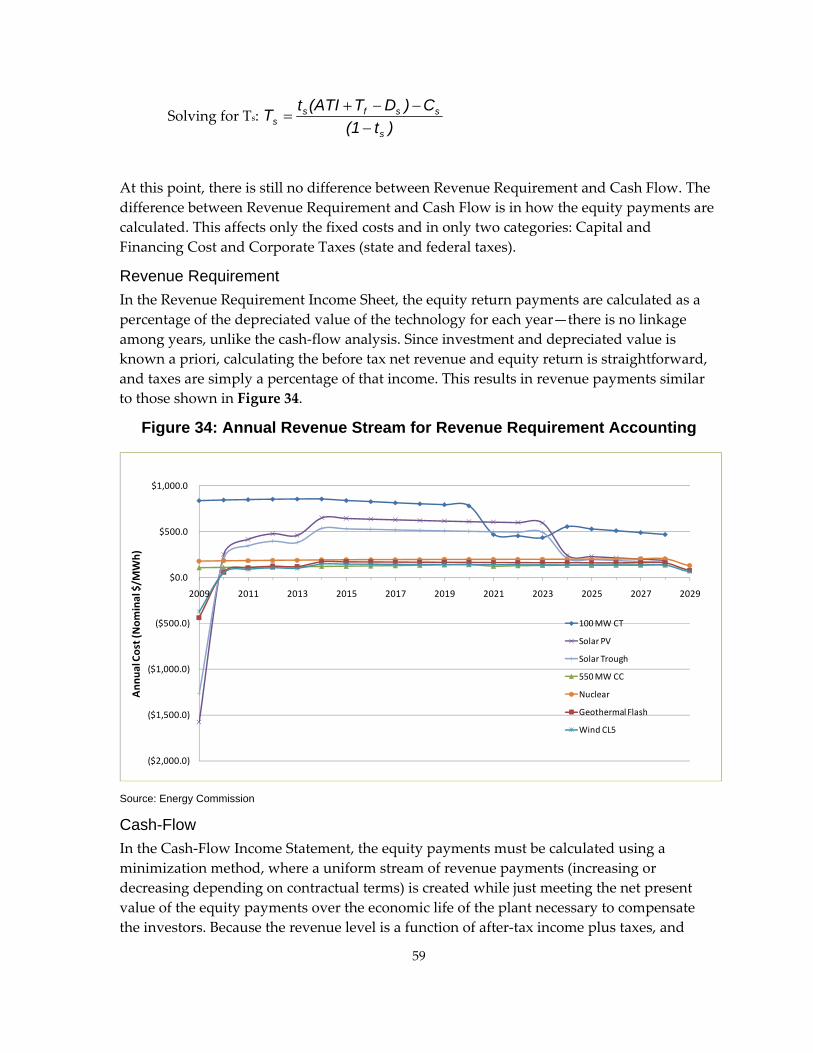
Solving for Ts: )t(1

C)DT(ATItTs

ssfss −

−−+=

At this point, there is still no difference between Revenue Requirement and Cash Flow. The difference between Revenue Requirement and Cash Flow is in how the equity payments are calculated. This affects only the fixed costs and in only two categories: Capital and Financing Cost and Corporate Taxes (state and federal taxes).

Revenue Requirement In the Revenue Requirement Income Sheet, the equity return payments are calculated as a percentage of the depreciated value of the technology for each year—there is no linkage among years, unlike the cash‐flow analysis. Since investment and depreciated value is known a priori, calculating the before tax net revenue and equity return is straightforward, and taxes are simply a percentage of that income. This results in revenue payments similar to those shown in Figure 34.

Figure 34: Annual Revenue Stream for Revenue Requirement Accounting

($2,000.0)

($1,500.0)

($1,000.0)

($500.0)

$0.0

$500.0

$1,000.0

2009 2011 2013 2015 2017 2019 2021 2023 2025 2027 2029

Ann

ual Cost (Nom

inal $/M

Wh)

100 MW CT

Solar PV

Solar Trough

550 MW CC

Nuclear

Geothermal Flash

Wind CL5


Cash-Flow In the Cash‐Flow Income Statement, the equity payments must be calculated using a minimization method, where a uniform stream of revenue payments (increasing or decreasing depending on contractual terms) is created while just meeting the net present value of the equity payments over the economic life of the plant necessary to compensate the investors. Because the revenue level is a function of after‐tax income plus taxes, and

59

taxes are a function of the before‐tax income, and the revenue amount must be a relatively level stream over the years, the model must solve for how equity income will vary among years so as to achieve the net present value target for equity return over the entire period, not one year at a time. In other words, unlike the revenue requirement method, the equity return in any year is not independent of the return in other years. The corresponding annual payments are shown in Figure 35.

Figure 35: Annual Revenue Stream for Cash-Flow Accounting

$0.0

$200.0

$400.0

$600.0

$800.0

$1,000.0

$1,200.0

2009 2011 2013 2015 2017 2019 2021 2023 2025 2027 2029

Ann

ual Cost (Nom

inal $/M

Wh)

100 MW CT

Solar PV

Solar Trough

Nuclear

550 MW CC

Geothermal Flash

Wind CL5


The Southern California Edison Cost of Generation Model, which is now being further developed by E3 for use in the CPUC MPR, uses the Excel© Goal Seek function to change the projected revenue by changing the contract price so that the net present value of the equity return equals the target equity return after paying taxes. The Black & Veatch (B&V) Cost of Generation Model, used for the Energy Commission’s Renewable Energy Transmission (RETI) studies, uses the Excel© Table function that makes a linear estimate of how the net revenue function changes with the contract price paid. Both Excel© functions produce similar results because the Goal Seek function uses a similar linear estimate method duplicated in the Table function setup. Staff elected to use the Table function similar to the B&V Cost of Generation model because it allows for automatic adjustment of the target contract price without having to run Goal Seek separately for each change in technology, assumptions, or scenarios. However, staff found that the change in net revenue was not a linear function over the full range of contract prices due to the more complex representation of expenses and taxes in the Energy Commission COG Model compared to the B&V RETI

60

61

model. Instead a piecewise linear function was created using the Table function to capture the nonlinear relationship.3

For two reasons, the revenue requirements and cash flow may not necessarily arrive at the same value. The first reason is since the revenue requirement calculates the annual revenue separately for each year, changes in the relationships among years does not affect the revenue requirement within an individual year. The annual revenue requirement is simply a function of the weighted average cost of capital that equals the discount rate used to calculate the levelized cost of capital. For the cash flow method, cost components are discounted by three discount rates—the interest rate for debt, the rate of return for equity for the profit, and the weighted average of these two for expenses. The resulting net present value of each of these streams of values is a nonlinear function of each discount rate. The sum of nonlinear functions does not equal the nonlinear function of the sums. The former is the cash flow method, the latter is the revenue requirement function. The second reason is that tax incentives typically are applied to nominal values asset values and income streams. Moving the net present value of income from one period to another can have secondary tax consequences that then change the revenue target, which in turn changes the tax looping back and forth. Typically the difference between the cash flow and revenue requirement results is not large, but it typically becomes significant where large tax incentives are applicable to a technology.

Overhaul Worksheet The Overhaul Worksheet is used only where component Variable O&M costs are calculated. At present, this is being done for the gas‐fired technologies, only. All other technologies have their Variable O&M reported as a single value.

The Overhaul Worksheet requires special treatment due to the inclusion of irregular maintenance intervals. In addition, the COG Model has a special requirement of having to develop Base Year values for use in the Income Statement Worksheet. This section describes how these irregular maintenance costs are converted into the necessary Base Year values for use in the Income Statement Worksheet.

The Income Statement Worksheet has an item called Variable O&M, which requires Base Year dollars as a starting point for its calculations. The Base Year is the most recent year for which there is known data, and is therefore the initial point of calculation. Variable O&M has several component costs that are calculated in the Data 2 worksheet, and then combined together to get the total Base Year Cost. Four of these components are not readily available in Base Year dollars and require a special—somewhat subtle—treatment to be converted to base year dollars:

3 The Table function calculation can be found on the Income_Cash Flow worksheet in the model, starting at cell B167.

62

• Major Overhaul Costs

• Minor Overhauls Costs

• Air Emission Equipment Replacement Costs

• Water Treatment & Cooling Equipment Costs

The Income Statement Worksheet takes the Base Year value and escalates it to cover Real Escalation (O&M Escalation & Labor Escalation) and Nominal (Historical & Forward) Inflation. It then calculates the Present Values of all these yearly values. And then finally calculates the Levelized Cost.

The Overhaul Worksheet first calculates the PV of the irregular maintenance, and then calculates a payment value, which is the necessary Base Year Value.

PMT((1+RealDiscountRate)/(1+OMEscalation)‐1, BookLife, SUM(E5:AE5) /(1+DiscountRate))* ((1+InflationRate)*(1+OMEscalation)) /((1+HistInflationRate)*(1+OMEscalation))(StartYr‐BaseYr)

For descriptive purposes, this can be simplistically represented as:

PMT(InterestRate, BookLife, PV)/ ((1+HistInflationRate)*(1+OMEscalation))(StartYr‐BaseYr)

The division of term in the second line which is the inflation from Base Year to Start year, ((1+HistInflationRate)*(1+OMEscalation))(StartYr‐BaseYr), is easily understood. That is, since multiplying the Base Year value by this term inflates the value to the Start Year, dividing by this same value deflates a Start Year value back to the Base Year. The explanation of the necessary “InterestRate” is more subtle but it essentially takes the Payment Value back to the Start Year. That is, it has to undo the Inflation and Real Escalation so that these values can be reconstructed in the Income Statement Worksheet. It does this by first reducing the Discount Rate by the Inflation Rate, which gives us Real Discount Rate, which is the real portion of the Discount Rate. Mathematically, the Real Discount Rate is constructed as follows:

(1+RealDiscountRate) = (1+DiscountRate) / (1+Inflation) RealDiscountRate = [(1+DiscountRate) / (1+Inflation)] ‐ 1

Similarly the Real Escalation must be removed:

(1+InterestRate) = (1+RealDiscountRate) / (1+OMEscalation)

InterestRate = [(1+RealDiscountRate) / (1+OMEscalation)] ‐ 1

This final manipulation will be recognized by some as calculating the Asset Rental Value (Carlton and Perloff 1990), but definitions are of less importance here than understanding the intent of the manipulations. One way to help understand this is to realize that if the

63

Present Value calculated on the Overhaul Worksheet could be moved directly to the Present Value cell on the Income Statement, all this manipulation would not be necessary. However, it would create an inconsistency in the format and would be complicated by the fact that there are several components of Variable O&M that must be first be added together and then divided by annual energy for this to be complete.

The following is a more rigorous treatment of this same issue, which will be helpful to those that are comfortable with mathematics but will simply be ponderous to others. The procedure first shows the mechanism of the Income Statement Worksheet and then explains how the Overhaul Worksheet prepares the Present Values of the Overhaul Worksheet to create the necessary Base Year value.

In the Income Statement Worksheet, the model goes through the following steps. The inflation is first calculated from the Base Year to the Start Year (In Service Year), using HistInflation for general inflation and RealEscalation to cover the real component of Escalation. The total inflation of Variable O&M is therefore calculated as:

((1+HistInflationRate)*(1+RealEscalation))(StartYr ‐ BaseYr)

It is then inflated year by year from the Start Year to the end of the period (typically 20 years, such that the exponent assumes values from 0 to 19):

((1+InflationRate)*(1+RealEscalation)(Year ‐ StartYr)

For a Base Year value designated herein as BaseYearVarO&M, each yearly value can therefore be calculated as:

BaseYearVarO&M*[(1+HistInflationRate)*(1+RealEscalation)](StartYr ‐ BaseYr)* [(1+InflationRate)*(1+RealEscalation)](Year ‐ StartYr)

If the following substitutions are made, this formula can be simplified for illustration:

a = BaseYearVarO&M

b = [(1+HistInflationRate)*(1+RealEscalation)](StartYr – BaseYr)

c = [(1+InflationRate)*(1+RealEscalation)]

Using the distributive law, the annual costs can then be represented by the formula:

Variable O&M = a * b * (c0+c1+c2+c3 +c4+c5………… cn‐1+cn)

And the Present Value can be calculated using Discount Rate “D” as:

Present Value of a * b * (c0+c1+c2+c3 +c4+c5………… cn‐1+cn) = a*b*Present Value of (c0+c1+c2+c3 +c4+c5………… cn‐1+cn)

= a*b*{(c0/(1+D)0 +c1/(1+D)1 + c2/(1+D2 + c3/(1+D)3+ c4/(1+D)4 +c5/(1+D)5 ………….. cn‐1/(1+D)n‐1 +cn/(1+)Dn} / (1+D)

64

= a*b*{[c/(1+D)]0+[c/(1+D)]1+[c/(1+D)]2+[c/(1‐D)]3+[c/(1+D)]4+[c/(1+D)]5+ …………. [c/(1+D)]n‐1+[c/(1+D)]n}/ (1+D)

This is mathematically equivalent to: (1‐vn)/(1/v‐1), where v =c/(1+D)

= a*b* {1‐ [c/(1+D)]n / 1/ [c/(1+D)] ‐1}

= a*b* {1‐ [c/(1+D)]n / [(1+D/c)] ‐1}

If c/(1+D) can be replaced with a term called EquivDiscountRate = i, then

(1+i) = (1+D)/c = (1+D)/ ((1+InflationRate)*(1+RealEscalation))

i = [(1+D)/ [(1+InflationRate)*(1+RealEscalation)] ‐1

Present Value = a*b* {1‐ [c/(1+D)]n/ [(1+D/c)] ‐1}

= a*b* {1‐ [1/(1+i)]n / [(i ‐1)}

Solving for a gives us the inverse of PV, which is a Levelized payment (PMT):

a =1/b * 1/ {1‐ [1/(1+i)]n / [(i ‐1)}= 1/b * 1/ PV= 1/b * PMT

Or in Excel terminology:

a =1/b * PMT(i, Life, PV)

BaseYearVarO&M =1/[(1+ HistInflationRate)*(1+RealEscalation)](StartYr‐BaseYr) * PMT(i, Life, PV)

The PV of irregular costs is calculated in the Overhauls Worksheet, and then the Payment Value is also calculated, using traditional PV techniques. This PV is then calculated using this formula, giving the cost in Start Year dollars. And finally, that value is divided by the escalation, [(1+HistInflationRate)* (1+RealEscalation)(StartYr‐BaseYr), to bring the value back to Base Year dollars.

Table 2 and Figure 36 illustrate how this works.

65

Table 2: Sample Overhaul Calculation

Nominal Discount Rate 10% Inflation Rate 2% Real Escalation Rate 0.5% Effective Discount Rate 7.31%

Year

Nominal Cash Flows w/Real

Escalation Rate

Levelized Cash Flows

with Nominal Discount Rate

Levelized Cash Flows

with Effective Discount Rate

LCFs w/RDR Escalated at

Inflation + Real 1 0.00 $20.49 $17.28 17.28 2 0.00 $20.49 $17.28 17.72 3 0.00 $20.49 $17.28 18.16 4 0.00 $20.49 $17.28 18.62 5 110.42 75.42 $20.49 $17.28 19.08 6 0.00 $20.49 $17.28 19.56 7 0.00 $20.49 $17.28 20.05 8 0.00 $20.49 $17.28 20.56 9 0.00 $20.49 $17.28 21.07 10 125.00 53.01 $20.49 $17.28 21.60 11 0.00 $20.49 $17.28 22.15 12 0.00 $20.49 $17.28 22.70 13 0.00 $20.49 $17.28 23.27 14 0.00 $20.49 $17.28 23.86 15 141.49 37.26 $20.49 $17.28 24.45 16 0.00 $20.49 $17.28 25.07 17 0.00 $20.49 $17.28 25.70 18 0.00 $20.49 $17.28 26.34 19 0.00 $20.49 $17.28 27.00 20 160.16 26.19 $20.49 $17.28 27.68 NPV-Nom $174.43 $174.43 $174.43 $174.43


Figure 36: Levelized Cash Flows-Periodic Costs

LCFs w/RDR Escalated at Inflation + Real

Levelized Cash Flows with Effective DiscountRate

Levelized Cash Flows with Nominal DiscountRate

Periodic Annual Costs

180

160

140

120

100

80

60

40

20

0

Years20191817161514131211109 8 7 6 5 4 3 2 1

$100

$90

$80

$70

$50

$60 $/Year

$0

$10

$20

$30

$40

160.16

110.42

125.00

141.49


66

67

Glossary

Acronym Definition

AFUDC allowance for funds used during construction

BETC business energy tax credit

Btu British thermal unit

California ISO California Independent System Operator

CC combined cycle

COG Model Cost of Generation Model, Version 2

CT combustion turbine

DCR debt coverage ratio

EBITDA earnings before interest, taxes, depreciation and amortization

EFOR equivalent forced outage rate

EMDH equivalent maintenance duration hours

Energy Commission California Energy Commission

EPDH equivalent planned duration hours

ERC emission reduction credit

ESDH equivalent scheduled duration hours

ESOF equivalent scheduled outage factor

FO forced outage

FOH forced outage hours

FOR forced outage rate

FTE full time equivalent

GADS generating availability data service

GDA geothermal depletion limit

GW/GWh gigawatt/gigawatt-hour

IEPR Integrated Energy Policy Report

IOU investor-owned utility

kW/kWh kilowatt/kilowatt-hour

68

LC levelized cost

MACRS modified accelerated cost recovery system

MMBtu million British thermal units

MO maintenance outages

MOH maintenance outage hours

MOR maintenance outage rate

MW/MWh megawatt/megawatt-hour

NCF net capacity factor

NOx nitrogen oxide

NPV net present value

O&M operation and maintenance

PH period hours

PM10 particles of 10 micrometers

PMT payment

PO planned outages

POH planned outage hours

POU publicly owned utility

PV present value

QFER Quarterly Fuel and Energy Report

RECLAIM regional clean air incentives market

REPI renewable energy production incentive

REPTC renewable energy production tax credit

RS reserve shutdowns

RTC RECLAIM trading credits

SCAQMD South Coast Air Quality Management District

SCR selective catalytic reduction

SH service hours

SL straight line

69

SOF scheduled outage factor

SOH scheduled outage hours

SOR scheduled outage rate

SOx sulfur oxide

TDMA tax deduction for manufacturing activities

UO unplanned outage

UOH unplanned outage hours

WACC weighted average cost of capital

CSI California Solar Initiative

SGIP self-generation incentive program

FERC Federal Energy Regulatory Commission

A‐1

APPENDIX A: Definitions

Accumulated Depreciation: This is a running total of the year by year depreciation.

Accumulated Depreciation = Book Value/Rate Base * Sum (Cumulative Yearly Book Depreciation) through Year N

Acquisition Costs: Total costs for acquiring the necessary land for the plant and dedicated infrastructure.

Acquisition Costs = Total Acres * Cost Per Acre

Ad Valorem Tax: Also called as Property taxes. In California, property tax is assessed differently based on ownership. Utility‐owned plants pay based on the value assessed by the State Board of Equalization, and is set to the Net Depreciated Book Value. The value reflects the market value of the asset, but may not increase in value at a rate faster than 2 percent per annum per Proposition 13. Municipal‐owned plants are exempted from paying property taxes, but may pay a negotiated in‐lieu fee. The calculation of Ad Valorem for any one year is:

If Owner Type = Merchant, then:

Ad Valorem Tax = Ad Valorem Tax Rate* Installed Cost (Year Calculation Is Done) *BOE Property Tax Depreciation Factor (1+ Forward Inflation Rate)(Year Calculation Is Done ‐Start Yr)

If Owner Type = IOU, then:

Ad Valorem Tax = Ad Valorem Tax Rate* Book Value/Rate Base

Air Control Annual Consumables‐Catalyst: The cost of the consumable inputs (for example, ammonia) used in the air emission control device, usually selective catalytic reduction (SCR).

Air Emissions Control Technology Capital Costs: It is the Capital Cost of purchasing and installing the Air Emissions Control Technology Equipment.

Air Emissions Control Technology Capital Costs = Air Emissions Control Installation Cost * Gross Capacity*1000

Allowance for Funds Used During Construction (AFUDC) Rate: The cost of the construction loan, insurance and taxes that are associated with construction period of the power plant. These costs are not recovered immediately through rates or sales, but are accumulated and recovered later along with the total capital investment. The AFUDC rate is usually set equal to the weighted average cost of capital (WACC), which is the case in the Energy Commission’s COG Model.

A‐2

Annual Average Heat Rate (Btu/kWh): A measure of the efficiency of power plants. It is the amount of heat supplied in Btu’s to generate 1 kWh of electricity. The smaller the heat rate the greater the efficiency. The efficiency of a power plant can be calculated as 3,413 divided by the heat rate (3,413 being the conversion factor to convert 1 kWh into Btu). The model uses heat rates based on actual performance, primarily as reported in the Energy Commission’s QFER database The reported annual fuel use (Btu) is divided by the annual energy (GWh).to get the Annual Heat Rate Therefore, heat rate variability and start‐up fuel are automatically captured.

See Definition below.

Annual Average Operating Heat Rate Net of Startups (Btu/kWh): Although this quantity does not affect the calculation of Heat Rate in the COG Model as explained above, it is provided as a convenience to the COG Model user, in order to estimate the effect of start‐ups on the Average Annual Heat Rate. Typically, this is small enough as to not be important, but sometimes it becomes significant for a combustion turbine. In any case, the effect is reported in the model should the user want to be cognizant of it.

Average Operating Heat Rate (Net Of Startups) = {(Annual Average Heat Rate*Gross Capacity /1000)* Operational (Service) Hours/Year– Start Up Fuel Use * Number Of Annual Starts)} / Gross Capacity /1000* Operational (Service) Hours/Year

Annual Capacity Degradation Rate (percent): The annual average rate at which a power plant loses peak generating capacity, averaged over the expected lifetime of the facility. The rate typically is small initially, but accelerates with age. This degradation can be offset by regular maintenance and overhauls. Although this rate varies over time, it is captured in the COG Model as a constant value throughout the life of the project. This is explained in more detail in Chapter 4 of the User’s Guide.

Annual Fuel Use: The estimated annual fuel used by a power plant.

Annual Fuel Use = Gross Capacity/(1+ Annual Capacity Degradation Rate) (Year Calculation Is Done – Start Yr) * Average Percentage Output*Operating Hours/Year/1000 *Average Operating Heat Rate * (1+Heat Rate Degradation)(Year Calculation Is Done – Start Yr) + Start‐Up Fuel * Number Of Annual Starts.

Annual Heat Rate Degradation: The annual increase in heat rate due to aging of the equipment is called Heat Rate Degradation, but is offset by periodic maintenance. Similar to the Capacity Degradation Rate, the Heat Rate Degradation Rate is given as a singular average value. In the COG Model, this makes heat rate and fuel consumption increase over time, but does not affect output (MW), which remains constant—unless annual capacity degradation rate is entered in the model.

A‐3

Annual Salary with Overhead ($): Annual Salaries with overhead included. This is calculated in the COG Model by applying an overhead multiplier.

Annual Salary w/ Overhead = {(Manager Full Time Equivalent (FTE)* Manager Salary + Plant Operator FTE * Plant Operator Hrs* Plant Operator Wage + Mechanics FTE * Mechanics Hrs * Mechanics Wage + Laborer FTE * Laborer Hrs * Laborer Wage + Support Staff FTE * Support Staff Hrs * Support Staff Wage)}* Overhead Multiplier

Annualized Air Emissions Replacement Cost: The Levelized Cost of replacing Air Emission equipment. This is calculated first as actual yearly costs, then as a Present Value of those annual costs, and then finally as a Levelized Cost. In Excel terminology the actual calculation is:

Annualized Air Emissions Replacement Cost = ‐PMT((1+ Real Discount Rate)/(1+OM Escalation)‐1, Book Life, Sum(Intermittent Values)/ (1+Discount Rate))* ((1+ Inflation Rate)* (1+OM Escalation))/((1+ Historical Inflation Rate)* (1+OM Escalation) ^(StartYr‐BaseYr)

Annualized Water Cooling Replacement Cost: The Levelized Cost of replacing Water Cooling equipment. This is calculated first as actual yearly costs, then as a Present Value of those annual costs, and then finally as a Levelized Cost. In Excel terminology the actual calculation is:

Annualized Air Emissions Replacement Cost = ‐PMT((1+ Real Discount Rate)/(1+OM Escalation)‐1, Book Life, Sum(Intermittent Values)/ (1+Discount Rate))* ((1+ Inflation Rate)* (1+OM Escalation))/((1+ Historical Inflation Rate)* (1+OM Escalation) ^(StartYr‐BaseYr)

Asset Rental Price: An alternative way of valuing property. For example, if a company owned a truck, it could value the truck at the same price it could rent the truck for. This is explained in detail in Attachment B.

Asset Rental Rate = Foregone Interest + Depreciation – Price Appreciation (or Depreciation)

Average Annual Energy (GWh): This is calculated at three points: power plant low side of the uplift transformer, the high side of the uplift transformer and the load center. This would be calculated as the capacity at each point times the operating hours times the average percent output except for the fact that this is the point in the COG Model where the effect of capacity degradation is captured. This is a complex calculation that is described in Chapter 4.

Average Percentage Output (percent): Expected average available capacity during hours of operation (for example, 100 percent for a Combined Cycle Unit, 66 percent for a Wind Unit, 100 percent for a combustion turbine even if unit is operated only during peak summer hours), including any periods of derated operation in this factor.

A‐4

Base Year: The most recent year for which the power plant data is available. Data for subsequent years is scaled from the Base Year using inflation rates.

Before Tax Income (Operating Income or [EBITDA]): This means “Earnings Before Interest, Taxes, Depreciation and Amortization,” but after all product/service, sales and overhead costs are accounted for. It is also sometimes referred to as Operational Cash Flow or Operating Income and it serves as a sort of starting point to solve the problem that the models does not inherently compute revenues because no “market price” is provided. Instead, the revenues are computed on the assumption that the revenues just equal those required to make the power plant financially viable under the assumed terms included in the model. It is solved as the simultaneous solution of equations and is explained within the User’s Guide. The formula in all its complexity is:

Before Tax Income = After Tax Return On Debt & Equity + State Taxes + Federal Taxes

Also,

Before Tax Income = Revenue – Operating Expenses

Book Depreciation: An accounting procedure that allocates the cost of a fixed asset over the estimated useful life of the asset. It is the amount of expense charged against earnings by a company to write off the cost of a plant or machine over its useful life, giving consideration to wear and tear, obsolescence, and salvage value. If the expense is assumed to be incurred in equal amounts in each business period over the life of the asset, the depreciation method used for state taxes is straight line (SL), and for federal taxes is MACRS tables.

If Owner Type =ʺMerchant”, Book Depreciation = 0

If Owner Type = “IOU, Municipal”,

Book Depreciation = Installed Cost (Start Year) * Book Depreciation Rate

Book Depreciation Rate: The rate at which book depreciation is collected. In the COG Model, this is Modified Accelerated Cost Recovery System for federal and 150 percent of declining balance for state.

Book Life (Years): The projected life of an asset upon which a depreciation schedule is based. From an accounting perspective, this is the period over which investors expect to recover their investments plus returns. The actual life of the power plant will likely exceed this by a number of years.

Book Value: A businessʹ historical cost of assets less liabilities. The book value of a stock is determined from a companyʹs records by adding all assets (generally excluding such intangibles as goodwill), then deducting all debts and other liabilities, plus the liquidation price of any preferred stock issued. The sum arrived at is divided by the number of common shares outstanding and the result is the book value per common share. Book value of the assets of a company may have little or no significant relationship to market value. Tangible

A‐5

Book Value is different than Book Value in that it deducts from asset value intangible assets, which are assets that are not hard (for example, goodwill, patents, capitalized start‐up expenses and deferred financing costs). Economic Book Value allows for a Book Value analysis that adjusts the assets to their market value. This valuation allows valuation of goodwill, real estate, inventories, and other assets at their market value. Book Value is also called Rate Base. See Rate Base.

Business Energy Tax Credit (BETC): A tax credit that is available to businesses and is applicable to merchant facilities only. See Appendix D.

Byproduct Revenues and Costs: Incidental income and costs associated with the power plant operation.

Capacity and Energy: Capacity is the ability to generate, store or receive Energy. This can be more vividly illustrated in terms of a specific example: an electrical generation power plant, where capacity (MW) is the ability to generate energy (GWh). If a power plant with a Capacity of 1000 megawatts (MW) operates for one hour, it will generate 1000 megawatt‐hours (MWh) of Energy ‐ or 1 Gigawatt‐hour (GWh). If it operates for one year (8,760 hours) at this Capacity, it will produce 8,760 GWh of Energy.

Capital & Financing (Construction) Costs ($/kW‐Yr): The costs of purchasing, installing and financing a power plant. It includes the cost of equipment and land purchases, any Emission Reduction Credits, the construction loan and the sales taxes. All these costs are ultimately financed through Debt and Equity, such that these costs can be defined as follows:

Capital & Financing Costs = Debt Payment +Equity Recovery

However, in the COG Model, this cost quantity is calculated in the Data 2 worksheet as the sum of the Instant Costs converted to annual construction costs that are adjusted for inflation and sales taxes.

Capital Construction Costs By Year ($): The construction takes place over a period of years. So the Capital Construction Costs for each year is the construction cost in the year along with the financing (AFUDC) associated with the construction loan for that year. The Excel formula is calculated as:

Capital Construction Costs By Year = Cost %/Year * Total Instant Capital Cost * IF(Months In Construction Year>0,(1+AFUDCRate/(24/ Months In Construction Year)),0)+ Cumulative Construction Costs By Year *(1+ AFUDC Rate),Total Instant Capital Cost)*((1+Historical Inflation Rate)*(1+Capital Cost Escalation Rate))^(Start Yr‐Base Yr)

Capital Structure (percent): This refers to the percentage of financing a power plant that is raised through equity as opposed to debt financing. Also, it’s the permanent long‐term financing of a company. Capital structure normally includes common and preferred stock, long‐term debt and retained earnings. It does not include accounts payable or short‐term

A‐6

debt. Table A‐1 is a summary of the present (2009 IEPR) capital cost data. For an IOU ownership, 52 percent of the Capital is raised through Equity and 48 percent through debt; the cost of equity is 11.85 percent, and the cost of debt is 5.40 percent.

Table A-1: Capital Cost Data

Capital Structure Cost Of Capital

Owner Type Equity Debt Equity Rate Debt Rate

Merchant Fossil 60.0% 40% 14.47% 7.49% Merchant Alternatives 40.0% 60% 14.47% 7.49% Default IOU 52.0% 48% 11.85% 5.40% Default POU 0% 100% 11.85% 5.40%

Source:

It should be apparent that either the percentage debt or percentage equity defines the other:

Debt Financed (%) = 1‐ Equity (%)

Commitment Fee: A fee paid to a debt financing entity to ensure that project financing is committed to a project.

Construction Insurance: The cost of insurance to cover the period during the construction of a power plant.

Consumption (Acre Foot/ MWh): The water used by the power plant per MWh.

Corporate Taxes (W/Credits) ($/KW‐Yr): The taxes, deductions and investment credits associated with the power plant. These are state and federal taxes. See State Taxes and Federal Taxes.

Corporate Taxes = State Taxes + Federal Taxes

Cost of Capital (percent): The cost to a company of acquiring funds to finance the company’s capital investments and operations. In general, there are two components, debt and equity. See Capital Structure, Debt and Equity.

Debt ($): Financing the cost of the power plant. Also, raising money through selling bonds, notes, or mortgages or borrowing directly from financial institutions. Borrowed money is paid in full, usually in installments, with interest. A lender incurs risk and charges a corresponding rate of interest based on that risk.

Debt Coverage Ratio: The debt coverage ratio is the ratio of the company’s operating profit to its expenses. This ratio indicates its ability to cover its expenses using its profits from operations. If it is low, the company might encounter difficulties meeting financial expenses

A‐7

out of its current activities. A high ratio indicates relatively low expenses and a good financial position.

A financial institution often will require before issuing debt that a financial prospectus show that the average debt coverage ratio (DCR) over the life of a loan will exceed a certain ratio, for example, 1.8 is common and a minimum DCR for any single year of a smaller ratio, for example, 1.5 is preferred.

Debt Payment: Periodic repayment of debt or a loan.

Debt Payment = Principal + Interest

Debt Rate (percent): The interest charged on a loan or debt issued.

Depreciation: Depreciation is the accounting of the deterioration of the physical and functional utility of a fixed asset due to usage and time. Depreciation can be explained in economic or accounting terms. The accounting depreciation methods are of two types: Book and Tax depreciation.

Discount Rate (percent): Used to calculate the present value of future cash flows as well as the levelized cost. The discount rate reflects not only the time value of money, but also the riskiness associated with the cash flows. The Discount Rate is calculated within the COG Model as the Weighted Average Cost of Capital (WACC).

Economic Life (years)—For accounting and depreciation, this term is synonymous with book life. More generally, this is the expected life of an asset over which it will be economically productive.

Effective Load Center Delivered Capacity: This is the same as average MW. It is used to find the equivalent constant MWs that would generate the equivalent energy. This is a useful mechanism to compensate for the variability of generation for units such as solar and wind. This is the Effective Operating Capacity delivered at the meter after being adjusted for transformer and transmission losses. This is the capacity measure appropriate for comparison to distributed generation and demand side management measures.

Effective Load Center Delivered Capacity= Load Center Delivered Capacity * Average Percent Output

Effective Operating Capacity (MW): Adjustment to Net Capacity that accounts for intermittent operational limits, for example, wind variation, hydro drought conditions, that reduce the expected plant capacity in any moment.

Effective Operating Capacity = Net Capacity *Average Percent Output

Emission Reduction Credits (ERC’s): Permit offsets purchases from other regional emitters to compensate for added emissions from a new power plant. The ERCs differ by air quality regulation district (for example, SCAQMD) and constituent pollutant (for example, NOx,

A‐8

SOx, PM10, and so forth.) The ERCs are for a one‐time purchase so the costs are spread over the book life of the asset similar to other capital expenditures.

Equipment Life (years): The estimated life of equipment. In the COG Model this is used to determine depreciation and the frequency of overhauls.

Equity ($): The net worth of a firm or corporation. Equity can be both common stock and preferred stock. Equity can come from selling of stock or other assets. The ownership shares of a corporation authorized by its articles of incorporation, including preferred and common stock. This is also known as capital stock or equity holdings and is expressed as ownership or percentage of ownership in a company or items of value (that is, assets and liabilities). These funds are acquired for construction and operation with repayment terms subject to income performance by the asset.

Equity Rate (percent): The rate that is used to calculate the cost of using a company’s equity holdings to finance the power plant – as opposed to using long‐term debt. This percentage in simplest terms is what it costs to pay the stock holders the necessary dividends plus expected capital appreciation, but it all includes all assets that can be used to raise money.

Equivalent Availability Factor (percent): A measure of a unit’s reliability. In simplest terms, it can be thought of as the percent of time that a power plant is available to generate power. That is, those hours when it is not on scheduled maintenance or down due to a forced outage. In the COG Model, it is defined as

A = (1‐FOR) (1‐SOF) Where: FOR = Forced Outage Rate SOF = Scheduled Outage Factor

The above formula is simplistic as it applies only to the case where a unit is either completely on or completely off – never derated due to partial equipment failure. Although this formula is used in the model, it really implies the more general case where derates exist, and Availability should be calculated as:

A = (1‐EFOR) (1‐ESOF) Where: EFOR = Equivalent Forced Outage Rate ESOF = Equivalent Scheduled Outage Factor

A‐9

Equivalent Forced Outage Rate (EFOR): A power plant’s rate if failure accounting for partial derates. FOR is simplistic in that it applies only to the cases where the power plant is either available at its full power or has completely failed. In actuality a power plant can be available at partial power; that is, derated. For this more complex case, the term EFOR is used to capture the effect of these derates.

EFOR =

Forced Outage Hours

+ Equivalent Forced Derated Hours

x

100% Forced Outage Hours

+

Service Hours

+

Equivalent Forced Derated Hours during Reserve Shutdowns (RS) Only

Equivalent Scheduled Outage Factor (ESOF): A measure of a power plant’s failure rate accounting for derates. Similar to EFOR, it accounts for scheduled maintenance that is performed while the plant is derated. Although annual maintenance, planned outage hours (POH) is typically performed with the power plant turned off, maintenance outages can be done during partial derates.

ESOF = (SOH+ESDH)/PH; Where: SOH = POH+MOH ESDH = EPDH+¬EMDH

Escalation In Capital Costs (percent): The cost of the power plant generally changes over time. This percentage value is the annual change in these costs. This escalation is used in the COG Model to translate known base year costs to the actual start year costs.

Federal Tax Depreciation: The depreciation allowance on capital assets provided in the Internal Revenue Code. The allowance is computed using the MACRS tax schedule.

Federal Tax Life (Years): The book life of the asset for purposes of computing federal tax depreciation and related tax items.

Federal Taxes: Taxes that the owner must pay to the federal government. These are calculated as follow:

If Owner Type =ʺMuni”, Federal Taxes = ‐REPI If Owner Type = “IOU, Merchant”, Federal Taxes = Federal Tax Rate*(After Tax Return On Debt & Equity ‐(Debt Interest+ Federal Tax Depreciation +TDMA+GDA‐–(BETC+REPTC)/ (1‐Federal Tax Rate))

Final Planned Operating Hours/Year: Expected Hours in a year the unit is planned to be operating. The expected hours of operation per year minus the Scheduled Outage Hours.

Final Planned Operating Hours/Year = Minimum (Planned Percent of Year Operational*8760, 8760 ‐ Scheduled Outage Hours.)

A‐10

Financial Transaction Costs: Fees collected by financial institutions related to issuing debt and raising equity to finance construction and operation of a power plant.

Fixed Costs ($/KW‐Yr or $/MWh): These are the costs for power plants that occur regardless of whether it operates or not. Fixed costs include capital cost (including the financing costs), insurance, ad valorem and corporate taxes (federal and state taxes). In other words, all costs except variable O&M and fuel costs.

Fixed Costs = Capital & Financing (Construction) Costs + Insurance + Ad Valorem Costs + Fixed O&M Costs + Corporate Taxes (W/Credits)

Fixed O&M Costs ($/KW‐Yr): These are the costs of operating and maintaining the power plant that occur regardless of how much the power plant operates. What is included in this category is not always consistent from one assessment to the other but always includes labor costs and the associated overhead. The most common characterization, and the one used in the Energy Commission’s COG Model, includes both staffing costs and non‐staffing costs. Non‐staffing costs are comprised of equipment, regulatory filings, and other miscellaneous direct costs. The Commission’s survey of costs found that for simple cycle and CC units, these costs ($/kW‐Yr) vary with the size of the plant. The formula used in the COG Model to calculate the first year values of fixed O&M is:

Fixed O&M/kW‐Yr (Base Year) = Annual Salary w/ Overhead+ Non Labor Fixed O&M/ Gross Capacity (MW)*1000

The annual cost is calculated in the COG Model as:

Fixed O& M Costs (Year Calculation Is Done) = (Fixed O&M/kW‐Yr (Base Year)*((1+Historical Inflation Rate)*(1+Labor Escalation))(Start Yr– Base Yr) * ((1+ Forward Inflation Rate)*(1 + Labor Escalation)) (Year Calculation Is Done ‐Start Yr)

Fixed Operating Expense: The sum of Fixed O&M Costs, Ad Valorem and Insurance.

Fixed Operating Expense = Fixed O&M Costs + Ad Valorem + Insurance

Forced Outage Hours: Forced outages (FO) are those outages where a plant must be taken out of service for unplanned repairs. The hours where a unit spends in this condition is called forced outage hours.

Forced Outage Rate (FOR): The power plant’s rate of failure. This calculation ignores the period during reserve shutdown (economic shutdown) as this period tells us nothing about how the plant performs—because it was not asked to perform we cannot know how it would have done. It is based solely on when it is called upon. The GADS formula for this is:

FOR = FOH / (FOH + SH) Where: FOH = Forced Outage Hours (Hours Of Failed Operation) SH = Service Hours (Hours Of Successful Operation)

A‐11

Forward Inflation Rate: It is the average annual inflation rate from the start year to the year calculation is done.

Fuel Consumption/Hour (MMBtu/Hr): The amount of fuel used by a power plant in Millions of Btu per hour.

Fuel Consumption/Hour = {Gross Capacity (MW)* Average Percentage Output *Annual Average Operating Heat Rate (Net of Start Up)}/1000

Fuel Cost ($/kW‐Yr): Fuel Cost is the cost of electricity. It is calculated as the Fuel Price ($/MMBtu) times the Fuel Use (MMBtu). Fuel Use is calculated as Gross MW times the Operating Hours times the Heat Rate (Btu/kWh). This is the major component of Variable Cost for fuel‐intensive sources for which fuel is purchased, for example, fossil fuels.

Fuel Costs ($/kW‐Yr) = Fuel Price ($/MMBtu)* Annual Fuel Use (MMBtu) Gross Capacity (MW)*1000

Full‐Time Equivalent (FTE): Equivalent number of employees working full time.

Geothermal Depletion Allowance: A federal tax deduction provided for exhausting or depleting (“depreciating”) a geothermal reserve. This allowance is similar to the oil depletion allowance in the federal tax code.

GDA = Minimum (Geothermal Depletion Limit * Tax On Return On Equity, Geothermal Depletion Percent * Equity Recovery)

Geothermal Resource Royalty Payment: When a company or individual enters into a geothermal lease with the United States Government, that company or individual agrees to pay a share (royalty) of the value of production to the United States.

Geothermal Resource Royalty Payment = 0.1* Return On Equity *Gross Capacity (MW) *1000

Gross Capacity (MW): The capacity of the power plant without parasitic load. That is, the capacity of the power plant before it has to provide power to serve the load associated with the power plant. See Net Capacity.

Historical Inflation Rate: It is the average annual inflation rate from the base year to the start year.

Inflation: The rate of change in a price index (for example, the Consumer Price Index) over a certain period that reflects a general increase in all prices so that the relative costs of different goods and services remain essentially the same. Alternatively, inflation reflects the percentage reduction in the purchasing power of a dollar over a specified period for example, a year.

Installed Costs (In‐Service Costs) ($/kW): The total cost of building a power plant. It includes not only the Instant Costs, but also the costs associated with the fact that it takes

A‐12

time to build a power plant. Thus, it includes a building loan, insurance, sales tax and property taxes—as well as the costs associated with escalation of costs during construction.

Installed Cost (Base Year) = Total Construction Cost * (1+CA Sales Tax) Gross Capacity*1000

Installed Cost (Start Year) = Total Construction Cost * (1+CA Sales Tax) (Gross Capacity*1000)*(1+ Historical Inflation Rate)Start Yr – BaseYr

Instant Costs ($/kW): The cost of a purchasing and building a power plant assuming that it could be built in an instant. In fact, the building may take several years and incur additional costs. See Installed Cost

Instant Cost (Base Year) = Total Instant Capital Cost (Gross Capacity*1000)

Instant Cost (Start Year) = Total Instant Capital Cost [(Gross Capacity*1000)*(1+Historical Inflation Rate)Start Yr – Base Yr]

Insurance: The cost of insuring the project which is paid as an annual premium.

If Owner Type =ʺIOUʺ, Insurance = Insurance %* Book Value Or Rate Base

If Owner Type = “Merchant, Municipal”, Insurance = Insurance %* Installed Cost (Year Calculation Is Done) * (1+ Forward Inflation Rate)(Year Calculation Is Done ‐Start Yr)

Labor Escalation: The escalation in plant operation labor costs above the escalation in general economy‐wide price levels or inflation.

Land Preparing Costs/Acre: The costs of preparing land before construction through clearing and infrastructure installation on a per acre basis.

Landfill Tipping Fees: The fees paid to dispose the Solid Waste.

Levelized Cost (LC): Levelized Cost is the singular most important objective of this model. It is the annual payment (same value all years) that is equivalent to all the costs incurred in the construction and operation of the power plant. If the Net Present Value of all these payments is calculated as NPV, then

LC = [NPV * I * (1+i)n] [(1+i)n ‐ 1].

The corresponding Excel formula is PMT (Discount Rate, Book Life, PV).

For a series of unequal payments, the Excel formula is PMT (Discount Rate, Book Life, NPV (Discount Rate, yearly value 1, yearly value 2, ...,yearly value n).

This is the same principle used in determining the mortgage payment on a house. A mortgage payment is a levelized payment to repay the lump‐sum loan amount, which is the equivalent of the net present value of the loan. For example, if the house cost $100,000, the

A‐13

expected term of the payment is 20 years and the interest rate of 5 percent, the annual house payment is $8,024.26.

Load Center: Load Center is the physical location where the power is being received under contract. The model must account for the losses between the where the power is generated, at the generator busbar (low side of uplift transformer), and where it is delivered at the Load Center.

Load Center Delivered Capacity: The available generating capacity delivered to the typical retail meter or “load center.” It is the capacity net of the power plant uplift transformer losses and the transmission losses.

Load Center Delivered Capacity = Net Capacity * (1‐ Transmission Losses)* (1‐Ancillary Services & Reserves)

Loan/Debt Term (Years): Length of loan for that portion of the financing of the power plant that is financed through long term debt. See Cost of Capital and Capital Structure.

MACRS Tax Tables: Federal tax depreciation tables reflecting the Modified Accelerated Cost Recovery System (MACRS). These depreciation methods apply to assets placed in service after 1986; less favorable than the earlier Accelerated Cost Recovery System (ACRS) system.

Major Overhaul: These are repairs that are extensive and are done less than annually, such as every 2.5 years. The calculation of these costs on an annual basis is quite complicated and is not shown here, but can be found in the Overhaul section of this User’s Guide.

Minor Overhaul: These are typically annual repairs that are much less extensive that major overhauls.

Major Overhaul Replacement Costs: It is the cost of replacing equipment associated with Major Overhauls.

Makeup Water: Water which is supplied (as to a steam boiler or cooling tower) to compensate for losses by evaporation and leakage.

Net (After ‐Tax) Income: Income after taxes are taken into account.

Net (After ‐Tax) Income = Before Tax Income ‐ Taxes

Net Capacity (MW): The capacity as it leaves the power plant structure, net of losses and providing station service. This is the usable power that leaves the power plant at the busbar and is sent over the transmission lines.

Net Capacity = Gross Capacity (1 – Plant Site Uses & Losses %)

Net Capacity Factor (NCF): This term is equivalent to Capacity Factor. Capacity Factor is calculated as the energy generated by the plant divided by the energy that could have been generated had it operated at full output for the entire year (8,760 hours). This denominator

A‐14

is an unlikely value as it assumes that there is no maintenance, no forced outages and no reserve shutdown during the entire year. In the COG Model it become equivalent to Availability for a base load unit because the COG Model assumes that there are no reserve shutdown hours. But for a CT, solar or wind unit, it will be less.

For a simple cycle unit (combustion turbine), it will be less as the Operational Hours are constrained to reflect its intended low capacity factor – this is done using Plant Percent of Year Operational. For a solar or wind unit, NCF will be less due to its Operating Capacity being derated to reflect the variability of its fuel source (sunlight for solar and adequate wind for wind units)

Net Capacity Factor (NCF) = Operational Hrs/Yr*Effective Operating Capacity (MW)/(8760*Net Capacity (MW))

Net Revenues ($/Lb): The revenue that is left after all costs are deducted.

Net Revenues = Revenues – (Processing Costs+ Shipping Costs)

Number of Annual Starts: The number of times a power plant is started during the year.

O&M Escalation: The real portion of O&M inflation. That is, the escalation in plant operation and maintenance non‐labor costs above or below the escalation in general economy‐wide price levels.

Operational (Service) Hours/Year: Number of hours in a year the power plant operates.

Operational Hours/Year = Planned Operating Hours/Year – Forced Outage Hours

Overhaul Labor (Hrs): The labor costs incurred in scheduled maintenance overhauls

Overhauls: Costs incurred for large‐scale scheduled maintenance. See Major Overhauls and Minor overhauls.

Overhead Multiplier: This multiplier is applied to the total labor salaries incurred to account for the added non‐salary costs such as benefits and employment taxes.

Period Hours (PH): GADS Terminology for the number of hours in a year.

Planned Percent of Year Operational: This factor is derived from either historical data or modeling results, both external to this model. Expected percent of year that unit is planned to be operating. This percentage times the Average Output During Operation will be the primary factors determining annual generation. For example: a solar plant may be operational 100 percent of the year with a 25 percent average output , a peaking unit will have a 100 percent average output with a 10 percent planned percent of year operational.

Plant Scheduling Costs: Costs incurred to sell and schedule power plant output to the grid, for example, for day‐ahead and real‐time sales to the California ISO. This cost can vary by technology and load‐following type (for example, peaking vs. baseload). This cost measure

A‐15

is appropriate for comparison to distributed generation and demand side management measures when computing costs at the Load Center.

Plant Losses (percent): The percentage of onsite load required to operate a power plant. This load typically includes pumps, lighting and other local services.

Predevelopment Expenses: Expenses incurred by the project developer in preparation for design, financing and construction.

Present Value (PV): The value of periodic payments discounted to the base year. Mathematically, each year’s value is multiplied by PV = 1 / (1+i)n, where i is interest (the value of money) and n is the number of years of discount. If the series of values are identical, the formula becomes PV = [(1 ‐ (1+i)n)] / i. Excel has a present value function called PV. If the series of payments are different, PV = 1 / (1+i)n must be multiplied against each yearly value – the corresponding Excel Formula is NPV.

Rate Base: The value of a regulated public utility and its operations as defined by its regulators and on which the company is allowed to earn a particular rate of return.

Book Value Or Rate Base = Installed Cost (Start Year) – Accumulated Depreciation.

Real Discount Rate: The real discount rate reflects the nominal or apparent discount net of inflation. The real discount rate is applied to present value calculations in economics, finance and engineering that use constant or real dollars. The proper discount rate to use depends on whether the benefits and costs are measured in real or nominal terms. This term is used in the model to facilitate the calculation of Overhaul Costs, Air Emissions, Water Treatment & Cooling Equipment Replacement Costs.

• A real discount rate that has been adjusted to eliminate the effect of expected inflation should be used to discount constant‐dollar or real benefits and costs. A real discount rate can be approximated by subtracting expected inflation from a nominal interest rate.

• A nominal discount rate that reflects expected inflation should be used to discount nominal benefits and costs. Market interest rates are nominal interest rates in this sense.

The real discount rate is calculated in the COG Model as follows:

Real Discount Rate = (1+Nominal Discount Rate) / (1+ Inflation Rate) ‐ 1

Renewable Energy Production Incentive (REPI): A tax credit that is available to Municipal facilities only. See Appendix D

Renewable Energy Production Tax Credit (REPTC): A tax credit that is available to Merchant & IOU facilities. See Appendix D

A‐16

Reservoir Management: Costs incurred in royalties and other fees for managing a geothermal steam or hot water reservoir or water rights associated with a reservoir or lake used to provide water to a hydropower plant.

Return Of Equity: A term used only by Investor Owned Utilities (IOUs), to break the more commonly used term “Return on Equity” into two parts Return on Equity and Return of Equity. Return of Equity is that portion that will exactly repay the sum of the initial investment without any profit.

If Owner Type =ʺIOUʺ, Return Of Equity = Equity Rate %* Book Depreciation

Return on Equity: In general, this term represents the portion of financing that is done through issuing stock as opposed to debt financing. For IOUs, it has a subtler meaning: It is the annual time value of money lent above and beyond the Return Of Equity. In other words, this is the profit that shareholders accrue from having made the initial investment. It is calculated differently based on ownership.

If Owner Type =ʺIOUʺ, Return On Equity = Equity Rate %* Book Value Or Rate Base*Equity Percent

If Owner Type = “Merchant”, Return On Equity =‐PMT((Equity Rate, Book Life, Equity Percent * Installed Cost Per kW)

Return on Ratebase: Measured as net income as a percentage of net book value (total assets minus intangible assets and liabilities). This is performance measure for a regulated utility.

Return on Ratebase = Return On Equity (Equity % * Book Value Or Rate Base)

Revenue Requirement: The revenues required to cover the total cost of constructing and operating a power plant: Operating Expenses, Taxes and Debt and Equity Payments. These types of utilities typically have posted prices prescribed by a regulatory commission or government council that do not directly reflect market forces.

Revenue Requirement = After Tax Return On Debt & Equity + Total Operating Expense+ Total Taxes

Reclaim Trading Credits & Mitigation Fees: South Coast Air Quality Management District (SCAQMD) RECLAIM Trading Credits (RTCs) and per pound of emission or per hour of operation mitigation fees paid to local air quality regulation districts. RTCs are bought and sold among several hundred industrial facilities to allow variations in NOx and SOx emissions from initial permitted levels. Mitigation fees are typically charged when a facility or power plant exceeds its permitted level of operation or emissions in a set period of time (for example, 12 months or a calendar year).

Scheduled Outage Factor (SOF): The ratio of SOH to the hours in a year (8,760). That is, the percentage of the year that a plant is on scheduled maintenance. If a plant has 876 hours of

A‐17

maintenance, then its SOF is 10 percent. This is more or less synonymous with the more commonly used modeling term Maintenance Outage Rate (MOR).

SOF = SOH/PH Where: SOH = POH+MOH

Scheduled Outage Hours: GADS define Scheduled Outages (SO) as the combination of Planned Outages (PO) and Maintenance Outages (MO). For those purposes when Maintenance Outage Hours (MOH) are still included with the Forced Outages (FO), the term Unplanned Outages (UO) is applicable.

Scheduled Outage (SO) = PO + Maintenance Outage (MO) Unplanned Outage (UO) = FO + Maintenance Outage (MO) Planned Outage (PO) = Yearly Planned Maintenance

The corresponding hours for Scheduled Outages (SO) and Unplanned Outages (UO) are Scheduled Outage Hours (SOH) and Unplanned Outage Hours (UOH). These are illustrated below, relative to Planned Outage Hours (POH), Maintenance Outage Hours (MOH) and Forced Outage Hours (FOH).

SOH = POH + MOH UOH = FOH + MOH

In the COG Model, only Scheduled Outage Hours are used.

Scheduler Costs: Costs for bidding and scheduling a power plant in the electricity market, for example, delivery of power to the California ISO).

Service Hours (SH): This is GADS terminology. In our model we use Operational (Service) Hours/Year.

Spark Spread: This is a measure of the financial viability of a power plant. In its common form, it compares the energy payments available to a power plant against its cost of operation (fuel cost times heat rate) – and is sometimes expressed as a heat rate difference. In the COG Model, it is characterized in a less common manner where the Revenue is compared against the cost of operation in the form of a heat rate difference. It is calculated of heat rate differences:

Spark Spread = [Revenue ‐ (Fuel Cost) * (Heat Rate)]*Gross MW/ Annual Energy

Start Year: The year that the power plant is in service and available to generate power for the grid. This is also the first year in the Present Value and Levelized Cost calculations. In the model Start Year is synonymous with In Service Year.

Start‐Up Fuel Use (MMBtu/Start): Prior to a thermal power plant being connected to the power system, it consumes fuel—most of which is associated with warming the power plant components, e.g. boilers. This warm up period can take anywhere from a few minutes to over a day, depending on the power plant. The fuel consumed is the Start‐Up Fuel.

A‐18

State Tax Depreciation: The depreciation allowance on capital assets provided in State law, in particular for California in the COG Model. The allowance is computed using the California tax schedules from the Franchise Tax Board.

State Tax Life (Years): The book life of the asset for purposes of computing State tax depreciation and related tax items.

State Taxes: Corporate income taxes that the owner must pay to the State Government, California in particular in the COG Model. These are calculated as below.

If Owner Type =ʺMuni”, State Taxes = ‐CSI – SGIP If Owner Type = “IOU, Merchant”, State Taxes = State Tax Rate*(After Tax Return On Debt & Equity+ Federal Taxes‐ (Debt Interest+ State Tax Depreciation )‐(CSI+SGIP)/ (1‐ State Tax Rate))

We included California Solar Initiative (CSI) and Self‐Generation Incentive Program (SGIP) in the formula for the User although the COG Model does not use them in the calculations.

Time To Major Overhaul: The period between major overhauls.

Time To Major Overhaul = Hours To Major Overhaul Operational (Service) Hours/Year

Total Acres: The total acreage of the power plant.

Total Acres = If (Isnumber (Acre Per MW), Acre Per MW * Gross MW, Acre Per Plant) +Additional Acreage

Total Air Emission Cost Conversion: Total Air Emission Costs can be calculated as below.

Air Emissions from Lbs/MWh to Tons/Yr = Lbs Air Emissions * Annual Net Energy (GWh) *1000 / 2000

Total Annual Air Emission Costs (Excluding Capital): The total annual costs of operating the Air Emission equipment.

Total Annual Air Emission Costs (Excluding Capital) = Calculated Air Emissions Replacement Cost + Air Control Annual Consumables Catalyst* Annual Net Energy (GWh)*1000 + Laborer Wage*Overhead Multiplier* Air Control Annual Labor (Hours/Year)

Total Annual Environmental O&M Costs: The sum of the annual Air Emissions Costs, Water Cooling Costs and Solid Waste Disposal Costs.

Total Annual Environmental Costs = Total Annual Air Emissions Costs (Excluding Capital) + Total Annual Water Treatment & Cooling Costs (Excluding Capital) + Total Annual Solid Waste Disposal Costs

A‐19

Total Annual Maintenance Costs: It is the sum of the Consumable Maintenance Costs, Periodic Routine Maintenance Costs, Other Routine Maintenance Costs, Well Field Costs, Scheduled Maintenance Costs & Other Unscheduled Maintenance Costs.

Total Annual Maintenance Costs = Total Consumable Maintenance Costs + Periodic Routine Maintenance Costs +Total Other Routine Maintenance Costs + Total Well Field Costs + Total Scheduled Maintenance Costs + Total Unscheduled Maintenance Costs.

Total Annual Solid Waste Disposal Costs: The total annual costs to dispose Solid Waste.

Total Annual Solid Waste Disposal Costs = Total Non – Hazardous Material Disposal Costs + Hazardous Material Disposal Costs

Total Annual Water Treatment Costs (Excluding Capital): The total annual costs of cooling the power plant net of water purchases. Water purchases are included in Fixed O&M, Other Operating Costs.

Total Annual Water Cooling Costs (Excluding Capital) = Calculated Water Treatment & cooling Replacement Cost + Water Control Annual Consumables Catalyst* Annual Net Energy (GWh)*1000 + Laborer Wage*Overhead Multiplier* Water Control Annual Labor (Hours/Year)

Total Component Costs ($): The cost for individual power plant components, for example, turbine sets, boilers, generators, control room. Reported costs may only show a sum total of all of these components.

Total Construction Costs ($): The total cost of a power plant that includes both the Instant Capital Cost ($) and the financing of the construction loan.

Total Consumable Maintenance Costs: Maintenance costs associated with consumption of materials, such as lubricating oils. These costs typically are incurred on a recurring, almost daily, basis. Either formula below can be used for calculating the Total Consumable Maintenance Cost.

Total Consumable Maintenance Costs = Consumable Maintenance Period * Total Consumable Cost Per Period,

Total Consumable Maintenance Costs = Oil Cost +Consumables Cost + Consumable Maintenance Labor

Total Cost Per Overhaul: The total cost of the overhaul.

Total Cost Per Overhaul = Major Overhaul Labor (Hrs) * Mechanics Wage/Hour* Overhead Multiplier + Major Overhaul Replacement.

Total Development Costs: Pre‐construction costs incurred by project developers for land acquisition and preparation and project financing. These costs are recovered within the Capital Cost expenditures.

A‐20

Total Development Costs = Predevelopment Expenses + Construction Insurance & Installation + Commitment Fee.

Total Environmental Costs ($/MWh): The annual costs environmental discharge control devices, such as selective catalytic reduction (SCR) devices to reduce air emissions and cooling water discharge control measures.

Total Environmental Costs = (Total Annual Environmental O&M Costs + Variable RTC’s & Mitigation Fees)/Load CenterEnergy (GWh)*1000

Total Environmental Control Installation Costs: The costs of installing necessary environmental discharge control devices, such as selective catalytic reduction (SCR) devices to reduce air emissions and cooling water discharge control measures. These costs are in addition to the Permitting Costs incurred to acquire the necessary environmental compliance fees.

Total Environmental Control Costs = Total Air Emissions Control Costs + Total Water Treatment & Cooling Control Costs

Total Hazardous Material Disposal Costs: The total costs associated with the disposal of Hazardous materials.

Total Hazardous Material Disposal Costs = Hazardous Material Tons/Year *(Hazardous Collection & Hauling Cost + Hazardous Landfill Tipping Cost)

Total Instant Capital Cost ($): The cost of purchasing and building a power plant assuming that it could be built instantaneously: Component Costs, Land Costs, Development Costs, Permitting Costs, Interconnection Costs, Total Environmental Controls Costs.

Total Instant Capital Cost = (Total Component Cost + Total Land Costs + Total Development Costs+ Total Permitting Costs + Total Interconnection Costs + Total Environmental Controls)* (1+Financial Transaction Costs* Debt Financed (%))

Total Interconnection Costs: Costs incurred to connect the power plant to the power grid beyond the busbar. These costs are highly project specific, but general values may be reported that represent “typical” cases for each technology.

Total Interconnection Costs = Transmission Interconnection + Fuel/Water/Sewer Costs

Total Land Costs: The costs to acquire and develop the land necessary to construct a power plant of a particular technology. The costs shown are typical for the setting in which a technology is most likely to be developed (for example, urban for fuel cells, ranch land for wind, industrial‐zoned for gas‐fired.) It is the sum of the Acquisition Costs and Total Land Preparation Costs.

Total Land Costs = Acquisition Costs + Total Land Preparing Costs

A‐21

Total Land Preparing Costs: The total costs associated with preparing the land in advance of the erection of the power plant.

Total Land Preparing Costs = Total Acres * Land Preparing Costs/Acre

Total Net Revenues = Total Net Revenues are calculated as follows

Total Net Revenues = Net Revenues * Net Capacity * Annual Production of Byproducts (Lbs/kW)

Total Non–Hazardous Material Disposal Costs: The total costs associated with the disposal of Non‐Hazardous materials.

Total Non‐Hazardous Material Disposal Costs = Non Hazardous Material Tons/Year * (Non Hazardous Collection & Hauling Cost + Non‐Hazardous Landfill Tipping Cost)

Total Operating Expense: The total of Fixed Operating Expense and Variable Operating Expense.

Total Operating Expense = Fixed Operating Expense + Variable Operating Expense

Total Operating Hours Over The Life Of The Plant: The projected total hours of plant operations over the economic life of the power plant. This value is used to compute the number of maintenance cycles required.

Total Operating Hours Over The Life Of The Plant = Equipment Life (Years) * Operational Hours/Year

Total Periodic Routine Maintenance Costs: The sum of periodic routine maintenance costs incurred on a regular, expected basis. These costs may be captured in the Total Routine Maintenance Costs (see below), but this category is included in the model for flexibility purposes, and for situations that may apply to specific technologies, for example, replacement of the fuel core in fuel cells.

Total Permitting Costs: Costs incurred in applying for necessary local‐use and environmental compliance permits, including direct permit fees. These costs do not include the costs of installing and operating Environmental Controls.

Total Permitting Costs = Local Building Permits + Environmental Permits + Emission Reduction Credits Costs

Total Return on Debt & Equity: The total net income over the entire amount, both debt and equity, invested in the power plant.

Total Return on Debt & Equity = Debt Payment + Equity Recovery +Total Taxes

Total Routine Maintenance Costs: These are costs for significant parts and labor incurred during the year. They are more frequent but less costly than Major and Minor Overhauls. In

A‐22

the COG Model, these costs are applicable to all technologies except Geothermal and Wind, which have their costs delineated under Total Other Routine Maintenance Costs.

Total Routine Maintenance Costs = Total Consumable Maintenance Costs + Total Periodic Routine Maintenance Costs +Total Other Routine Maintenance Costs + Total Well Field Costs

Total Other Routine Maintenance Costs: These costs similar in nature to the above defined Total Routine Maintenance Cost, with added categories for certain technologies such as Geothermal and Wind. The listed items are specific to the technologies as provided by technology specialists. Definitions of those items should be collected from such specialists, and are beyond the scope of this Guide.

Total Scheduled Maintenance Costs: The sum of the Major Overhaul Costs and the Minor Overhaul Costs. See Major Overhauls and Minor Overhauls.

Total Scheduled Maintenance Costs = Major Overhaul Cost + Minor Overhaul Cost.

Total Tax Rate: This is the total of the State and Federal Taxes.

Total Tax Rate = Federal Tax Rate*(1‐ State Tax Rate) + State Tax Rate

Total Unscheduled Maintenance Costs: Expected average annual costs for repairing a power plant after a forced outage or other unforeseen outage.

Total Unscheduled Maintenance Costs = Mechanics Wage/Hour * Overhead Multiplier * Hours of Labor + Parts Costs

Total Well Fields Costs: Costs incurred at geothermal plants for maintenance and operation of steam and hot‐water reservoir well fields.

Transformer Losses (percent): In the process of a transformer uplifting or down lifting the voltage, some of the power is lost. These losses are called Transformer Losses.

Transmission Losses (percent): Losses incurred in the transmission lines during the transmission of electricity, between the busbar and delivery to the distribution grid usually in the form of heat or a voltage drop.

Transmission Services ($/MW): Cost of connecting to the transmission grid and delivering power over that grid, typically paid to a transmission system owner under Federal Energy Regulatory Commission (FERC)‐approved tariffs.

Variable Costs ($/KW‐Yr Or $/MWh): Costs that change as a function of power plants use; that is, fuel costs and Variable O&M (Hourly labor, supply purchases). As the time horizon of the analysis expands, more costs become variable. More specifically for a power plant, these are all costs which are a function of the operation of the plant—if the plant has a zero capacity factor, then theoretically these costs are zero.

Variable Costs = Fuel Costs + Variable O&M

A‐23

Variable O&M Costs ($/MWh): Operation & Maintenance costs that are a function of the operation of the power plant (yearly maintenance and overhauls). In the Energy Commission’s COG Model, the annual costs are calculated by the following formula:

Variable O& M Costs ($/MWh)(Year Calculation Is Done) = (Variable O&M/MWh (Base Year) *((1+Historical Inflation Rate)*(1+ O&M Escalation)(Start Yr – Base Yr) )* ( (1+O&M Escalation)*(1+Forward Inflation Rate) (Year Calculation Is Done – Start Yr) )

To convert from $/MWh to ($/KW‐Yr):

Variable O& M Costs ($/MWh )*Annual Load Center Energy (GWh) Gross Capacity (MW)

Variable Operating Expense: The same as Variable Costs—the sum of Fuel Cost and Variable O&M.

Water Supply Costs ($/Acre‐Foot): The costs of acquiring water supplies in the listed region. Costs reported represent typical industrial water delivery rates found in the Regional Cost Differences report for the California ISO in 2002.

To convert the Water Supply Costs into ($/MWh):

Water Supply Costs = (Water Supply Costs/Acre Foot)* Water Consumption (Acre Foot)

Water Treatment & Cooling Control Technology Capital Costs: It is the Capital Cost of purchasing and installing the Water Treatment & Cooling Control Technology Equipment.

Water Treatment & Cooling Control Technology Capital Costs = Water Cooling Control Installation Cost * Gross Capacity*1000

Water Treatment & Cooling Control Technology—The method used to cool a power plant. Different technologies use different intensities of water consumed per MWh of output, with installation and operating costs increasing as less water is used.

Weighted Average Cost Of Capital (WACC): The average cost of financing the construction of a power plant. The weighted average is calculated by multiplying the percentage of the incremental capital used for financing that comes from debt instruments and equity sources by their respective interest rates.

WACC =Percent Equity * Cost of Equity( %) + Percent Debt * Cost of Debt(%)* (1‐ Total Tax Rate)

The WACC is also used as the AFUDC rate and the discount rate ‐ used to calculate the Present Value of future cash flows as well as the Levelized Cost.

Wheeling Charges ($/KWh): Cost of delivering power over the transmission grid, typically paid to a transmission system owner under FERC‐approved tariffs.

A‐24

APPENDIX B: Federal Tax Incentives Source : www.dsireusa.org

Figure B‐1 summarizes the presently available Federal tax credits. However, it should be kept in mind that these tax credits are subject to change, and may not be realizable by all power plants.

Figure B-1: Summary of Tax Credits—2009 IEPR

Notes:

1. GCC Production Credit separate from REPTC. Based on "refined coal" = $4.375/(13900 Btu/ton for anthracite / HR*(1+ParasiticLoad) for IGCC). Expiration date for ARRA ITC unclear

2. Geothermal ITC does not expire. Unclear as to whether the ARRA increased the ITC for geothermal to 30% until 2014, and whether self-sales are eligible

3. Solar ITC reverts to 10 percent in 2016

4. REPI payments scaled based on 2007 shares of paid to applications

Source: Aspen

B‐1

http://www.dsireusa.org/

1‐1

ATTACHMENT A: Reference for Degradation Factors

Pacific Group Electric Power LLC

Memorandum

From James L. Schoonmaker

DATE: Wednesday, December 07, 2005

TO: Will Walters

Aspen E.G.

SUBJECT: Gas Turbine Performance Degradation with Time

Below is a brief summary of the situation with regard to gas turbine and CC power plant degradation due to simple aging. The General Electric Technical Bulletin is typical of the current understanding, and is similar to views expressed by Siemens/Westinghouse, ABB and Mitsubshi.

Some general statements:

Degradation usually happens gradually over time. The root causes include deposit of airborne material – particularly silica – on turbine blades at high temperature, erosion/corrosion of blading due to other airborne salts – particularly sodium, maintenance practices such as regular blade washing – on line or offline, number of starts and operating hours. Occasional use of oil fuel also has major negative impact, as does poor air filtration and unusual airborne contaminant load.

1‐2

The usual degradation pattern is “saw tooth” shaped; from initial operation to the first hot gas inspections a modern frame turbine may lose 3 percent of its capacity and heat rate. The cleaning at the hot gas inspection will recover 1 ½ to 2 percent of original (leaving 1 to 1 ½ percent loss from initial operation). There will be a further 3 percent loss over the next 24,000 hours to the second gas path inspection, and cleaning will recover most, so at the end of the second inspection the machine will lose approximately 2 to 3 percent of its original capacity. This saw tooth shaped degradation continues until gas path parts are replaced to bring the machine to original performance – typically this never occurs in practice as machines have reached their useful life cycle by the time economics would become attractive.

The description above is typical of frame turbines in California at many locations. A turbine located near the ocean may experience 5 to 6 percent loss between hot gas inspections. A turbine near a steel mill in California suffered very serious losses in the first year. A desert environment machine properly filtered to protect against silica intrusion may experience 2 percent loss. Machines subject to frequent starting cycles may degrade more quickly than typical due to the moisture generated by cold temperatures in starting as well as differing chemistry on blade surfaces.

Typically aeroderivative turbines degrade on the high end of that of frame turbines, although repair by replacement allows easier correction of the degradation.

In a CC plant the gas turbines usually account for about 2/3 of the total plant output, so total plant performance degradation may be 2/3 or even less than gas turbines alone.

Below is the relevant portion of the Technical Bulletin reference:

General Electric Technical Bulletin GER-3567H

Last update 2000

General Electric proprietary material.

“All turbomachinery experiences losses in performance with time. Gas turbine performance degradation can be classified as recoverable or non‐recoverable loss. Recoverable loss is usually associated with compressor fouling and can be partially rectified by water washing or, more thoroughly, by mechanically cleaning the

1‐3

compressor blades and vanes after opening the unit. Non‐recoverable loss is due primarily to increased turbine and compressor clearances and changes in surface finish and airfoil contour. Because this loss is caused by reduction in component efficiencies, it cannot be recovered by operational procedures, external maintenance or compressor cleaning, but only through replacement of affected parts at recommended inspection intervals. Quantifying performance degradation is difficult because consistent, valid field data is hard to obtain. Correlation between various sites is impacted by variables such as mode of operation, contaminants in the air, humidity, fuel and diluent injection levels for NOx. Another problem is that test instruments and procedures vary widely, often with large tolerances. Typically, performance degradation during the first 24,000 hours of operation (the normally recommended interval for a hot gas path inspection) is 2 percent to 6 percent from the performance test measurements when corrected to guaranteed conditions. This assumes degraded parts are not replaced. If replaced, the expected performance degradation is 1 percent to 1.5 percent. Recent field experience indicates that frequent off‐line water washing is not only effective in reducing recoverable loss, but also reduces the rate of non‐recoverable loss. One generalization that can be made from the data is that machines located in dry, hot climates typically degrade less than those in humid climate.

ATTACHMENT B: Asset Rental Prices

2‐1

TURNING AN ASSET PRICE INTO A RENTAL RATE

2‐2

Cost of Generation Model

Documents

Transcript of Cost of Generation Model