Cost Minimization and the Cost Function · Cost Minimization and the Cost Function Juan Manuel...

Cost Minimization Second Order Conditions Conditional factor demand functions The cost function Average and Marginal Costs Geometry of Costs

Cost Minimization and the Cost Function

Juan Manuel Puerta

October 5, 2009


So far we focused on profit maximization, we could look at adifferent problem, that is the cost minimization problem. This isuseful for some reasons:

Different look of the supply behavior of competitive firmsBut also, this way we can model supply behavior of firms thatdon’t face competitive output prices(Pedagogic) We get to use the tools of constrained optimization

Cost Minimization Problem: minx wx such that f(x) = y

Begin by setting-up the Lagrangian: L(λ, x) = wx− λ(f (x)− y)Differentiating with respect to xi and λ you get the first orderconditions,

wi − λ∂f (x∗)∂xi

= 0 for i=1,2,...,nf (x∗) = y


Letting Df (x) denote the gradient of f (x), we can write the nderivative conditions in matrix notation as,

w = λDf (x∗)Dividing the ith condition by the jth condition we can get thefamiliar first order condition,

wi

wj=

∂f (x∗)∂xi

∂f (x∗)∂xj

, for i, j = 1, 2, ..., n (1)

1 This is the standard “isocost=slope of the isoquant” condition †2 Economic intuition: What would happen if (1) is not an equality?†


Source: Varian, Microeconomic Analysis, Chapter 4, p. 51.


Second Order Conditions

In our discussion above, we assume we “approach” the isoquantfrom below. Do you see that if your isoquant is such that theisocost approaches it from above there is a problem?

Other way of saying this is: if we move along the isocost, wecannot increase output? Indeed, output should remain constantor be reduced.

Assume differentiability and take a second-order Taylorapproximation of f (x1 + h1, x2 + h2) where hi are small changesin the input factors. Then,

f (x1 + h1, x2 + h2) ≈ f (x1, x2) + ∂f (x1,x2)∂x1

h1 + ∂f (x1,x2)∂x2

h2 +

(1/2)[∂2f (x1,x2)

∂x21

h21 + 2∂

2f (x1,x2)∂x1∂x2

h1h2 + ∂2f (x1,x2)

∂x22

h22]


Second Order Conditions

Since we assumed a move along the isocost,w1h1 + w2h2 = 0 = λ(f1h1 + f2h2) where the last equalityfollows from using FOC (wi = λfi)But in order to be at an optimum,f (x1 + h1, x2 + h2)− f (x1, x2) ≤ 0, which means that(

h1 h2)(f11 f12

f21 f22

)(h1h2

)≤ 0 (2)

for f1h1 + f2h2 = 0Generalizing to the n-factor case,

h′D2f (x)h ≤ 0 for all h satisfying wh = 0Where h = (h1, h2, ..., hn) is a quantity vector (a column vectoraccording to our convention) and D2f (x) is the Hessian of theproduction function.Intuitively, FOC imply that the isocost is tangent to the isoquant.SOC imply that a move along the isocost results on a reductionof output.


The second order conditions can also be expressed in terms ofthe Hessian of the Lagrangian

D2L(λ∗, x∗1, x∗2) =

∂2L∂λ2

∂2L∂λ∂x1

∂2L∂λ∂x2

∂2L∂x1∂λ

∂2L∂x2

1

∂2L∂x1∂x2

∂2L∂x2∂λ

∂2L∂x2∂x1

∂2L∂x2

2

Computing these derivatives for the case of our Lagrangianfunction L(λ, x) = wx− λ(f (x)− y)


The resulting is the Bordered Hessian

D2L(λ∗, x∗1, x∗2) =

0 −f1 −f2−f1 −λf11 −λf12−f2 −λf21 −λf22

It turns out that the sufficient conditions stated in (2) are satisfiedwith strict inequality if and only if the determinant of thebordered hessian is negative. Similarly, if you have n factors, thebordered Hessians for the n-cases should be negative


Difficulties

For each choice of w and y, there should be an optimum x∗ thatminimizes the cost of producing y. This is the ConditionalFactor Demand (Cf. factor demands in profit maximization)

Similarly, the Cost Function is the function that gives theminimum cost of producing y at the factor prices w.c(w, y) = wx(w, y)


As in the profit maximization case, there could be cases in whichthe first order conditions would not work

1 Technology not representable by a differential productionfunction (e.g. Leontieff)

2 We are assuming interior solution, i.e. that all the inputs are usedin a strictly positive amount. Otherwise, we have to modify theconditions according to Kuhn-Tucker,

λ∂f (x∗)∂xi− wi ≤ 0 with strict equality if xi > 0

3 The third issue concerns the existence of the optimizing bundle.The cost function, unlike the profit function, will always achievea minimum. This follows from the fact that a continuous functionachieves a minimum and a maximum on a compact (close andbounded) set. (more on that on the next slide)

4 The fourth problem is the issue of uniqueness. As we saw,calculus often ensures that a local maximum is achieved. Forfinding global maxima you have to make extra assumptions,namely V(y) convex.


More on why existence of a solution would not be aproblem in the cost minimization case?

Because we are minimizing a continuous function on a close andbounded set. To see this, wx is certainly continuous and V(y) isclosed by assumption (regularity assumption). Boundedness could beproved easily. Assume an arbitrary x′, then the minimal cost bundlemust have a lower cost, wx ≤ wx′. But then we can restrict to a subset{x in V(y):wx ≤ wx′}, which is bounded so long w� 0


Some Examples of Cost Minimization

Cobb Douglas with 2 inputs, f (x1, x2) = Axa1xb

2. †CES, f (x1, x2) = (xρ1 + xρ2)1/ρ. Homework!

Leontieff, f (x1, x2) = min{ax1, bx2}. †Linear, f (x1, x2) = ax1 + bx2. Illustration of the Kuhn-Tuckerconditions. †


2-input case

In the usual fashion, the conditional factor demand functionimply the following identities,

f (x(w,y)) ≡ y

w− λDf(x(w,y) ≡ 0

For the simpler 1-output, 2-input case, FOC imply

f (x1(w1,w2, y), x2(w1,w2, y)) ≡ y

w1 − λ∂f (x1(w1,w2,y),x2(w1,w2,y))∂x1

≡ 0

w2 − λ∂f (x1(w1,w2,y),x2(w1,w2,y))∂x2

≡ 0


As we did with the FOC of the profit maximization problem, wecan differentiate these identities with respect to the parameters,e.g. w1 †

∂f∂x1

∂x1∂w1

+ ∂f∂x2

∂x2∂w1≡ 0

1− λ[∂2f∂x2

1

∂x1∂w1

+ ∂2f∂x1∂x2

∂x2∂w1

]− ∂f∂x1

∂λ∂w1≡ 0

0− λ[ ∂2f∂x2∂x1

∂x1∂w1

+ ∂2f∂x2

2

∂x2∂w1

]− ∂f∂x2

∂λ∂w1≡ 0

Which can be written in matrix form as, 0 −f1 −f2−f1 −λf11 −λf21−f2 −λf12 −λf22

∂λ∂w1∂x1∂w1∂x2∂w1

≡ 0−10

Note that the matrix on the left is precisely the “BorderedHessian”


Recall the Cramer’s Rule, we can use it to solve for ∂xi/∂w1 †

∂x1∂w1

=

∣∣∣∣∣∣∣∣0 0 −f2−f1 −1 −λf21−f2 0 −λf22

∣∣∣∣∣∣∣∣∣∣∣∣∣∣∣∣0 −f1 −f2−f1 −λf11 −λf21−f2 −λf12 −λf22

∣∣∣∣∣∣∣∣Solving the determinant on the top, and letting H denote thelower determinant

∂x1∂w1

= f 22H < 0

In order to satisfy SOC, H < 0, which means that the conditionalfactor demand has a negative slope.


Similarly, you can use Cramer’s rule to solve for ∂x2∂w1

,

∂x2∂w1

=

∣∣∣∣∣∣∣∣0 −f1 0−f1 −λf11 −1−f2 −λf12 0

∣∣∣∣∣∣∣∣∣∣∣∣∣∣∣∣0 −f1 −f2−f1 −λf11 −λf21−f2 −λf12 −λf22

∣∣∣∣∣∣∣∣Carrying out the calculations,

∂x2∂w1

= −f2f1H > 0

Similarly, you can differentiate the identities above with respectto w2 to get 0 −f1 −f2

−f1 −λf11 −λf21−f2 −λf12 −λf22

∂λ∂w2∂x1∂w2∂x2∂w2

≡ 0

0−1


And using the Cramer’s rule again, you can obtain∂x2∂w1

= −f1f2H > 0

Compare the expressions for ∂x1∂w2

and ∂x2∂w1

. You will notice that asin the case of the factor demand functions, there is a symmetryeffect.

In the 2-factor case, ∂xi∂wj

> 0, means that factors are alwayssubstitutes.

Of course, this analysis is readily extended to the n-factor case.As in the case of the profit maximization problem, it is better touse matrix notation.


n-input case

The first order conditions for cost minimization are 1

f (x(w)) ≡ y

w− λDf (x(w)) ≡ 0

Differentiating these identities with respect to w,

Df (x(w))Dx(w) = 0

I− λD2f (x(w))Dx(w)− Df (x(w))Dλ(w) = 0

Rearranging this expression,(0 −Df (x(w))

−Df (x(w))′ −λD2f (x(w))

)(Dλ(w)Dx(w)

)= −

(0I

)

1We omitted y as an argument as it is fixed.


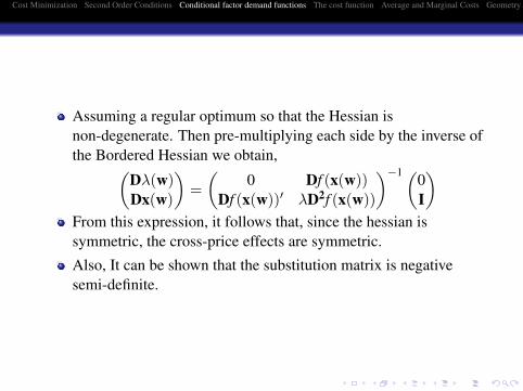
Assuming a regular optimum so that the Hessian isnon-degenerate. Then pre-multiplying each side by the inverse ofthe Bordered Hessian we obtain,(

Dλ(w)Dx(w)

)=(

0 Df (x(w))Df (x(w))′ λD2f (x(w))

)−1(0I

)From this expression, it follows that, since the hessian issymmetric, the cross-price effects are symmetric.

Also, It can be shown that the substitution matrix is negativesemi-definite.


The cost function

The cost function tells us the minimum cost of producing a levelof output given certain input prices.

The cost function can be expressed in terms of the conditionalfactor demands we talked about earlier

c(w,y) ≡ wx(w,y)Properties of the cost function. As with the profit function,there are a number of properties that follow from costminimization. These are:

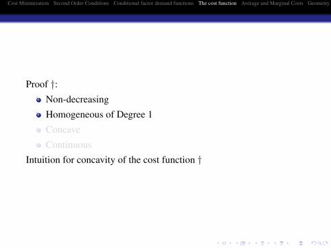
1 Nondecreasing in w. If w′ ≥ w, then c(w′, y) ≥ c(w, y)2 Homogeneous of degree 1 in w. c(tw, y) = tc(w, y) for y>0.3 Concave in w. c(tw + (1− t)w′) ≥ tc(w) + (1− t)c(w′) for

t ∈ [0, 1]4 Continuous in w. c(w, y) is a continuous function of w, for

w� 0


Proof †:Non-decreasing

Homogeneous of Degree 1

Concave

Continuous

Intuition for concavity of the cost function †


Shepard’s Lemma

Shepard’s Lemma: Let xi(w, y) be the firm’s conditional factordemand for input i. Then if the cost function is differentiable at(w, y), and wi > 0 for i = 1, 2, 3, ..., n then,

xi(w, y) = ∂c(w,y)∂wi

for i = 1, 2, ..., n

Proof †In general there are 4 approaches to proof and understandShepard’s Lemma

1 Differentiate de identity and use FOC (Problem set 2)2 Use the Envelope theorem directly (see next section)3 A geometric argument †4 A economic argument. At the optimum x, a small change in

factor prices has a direct and an indirect effect. The indirect effectoccurs through re-optimization of x but this is negligible in theoptimum. So we are left with the direct effect alone, and this isjust equal to x.


Envelope theorem for constrained optimization

Shepard’s lemma is another application of the envelope theorem,this time for constrained optimization.

Consider the following constrained maximization problem

M(a) = maxx1,x2 g(x1.x2, a) such that h(x1, x2, a) = 0

Setting up the lagrangian for this problem and obtaining FOC,∂g∂x1− λ ∂h

∂x1= 0

∂g∂x2− λ ∂h

∂x2= 0

h(x1, x2, a) = 0

From these conditions, you obtain the optimal choice functions,x1(a), x2(a) obtaining the following identity

M(a) ≡ g(x1(a), x2(a))


Envelope theorem for constrained optimization

The envelope theorem says that dM(a)da is equal to

dM(a)da = ∂g(x1,x2,a)

∂a |x=x(a) − λ∂h(x1,x2,a)

∂a |x=x(a)

In the case of cost minimization, the envelope theorem implies∂c(x,w)∂wi

= ∂L∂wi

= xi|xi=xi(w,y) = xi(w, y)

∂c(x,y)∂y = ∂L

∂y = λ

The second implication follows also from the envelope theoremand just means that (at the optimum), the lagrange multiplier ofthe minimization cost is exactly the marginal cost.


Comparative statics using the cost function

Shepard’s lemma relates the cost function with the conditional factordemands. From the properties of the first, we can infer someproperties for the latter.

1 From the cost function being non decreasing in factor pricesfollows that conditional factor demands are positive.∂c(w,y)∂wi

= xi(w, y) ≥ 02 From c(w, y) being HD1, it follows that xi(w, y) are HD03 From the concavity of c(w, y) if follows that its hessian is

negative semi-definite. From Shepard’s lemma it follows that thesubstitution matrix for the conditional factor demands is equal tothe Hessian of the cost function. Thus,

1 The cross price effects aresymmetric.∂xi/∂wj = ∂2c/∂wi∂wj = ∂2c/∂wj∂wi = ∂xj/∂wi

2 Own price effects are non-positive (∂xi/∂wi = ∂2c/∂w2i ≤ 0

3 The vectors of own factor demands moves “opposite” to thevector of changes of factor prices. dwdx ≤ 0


Average and Marginal Costs

Cost Function:c(w, y) ≡ wx(w, y)Let’s break up the w in fixed wf and variable inputs wv,w = (wf,wv). Fixed inputs enter optimization as constants.

Short-run Cost Function:c(w, y, xf) = wvxv(w, y, xf) + wfxf

Short-run Average Cost: SAC = c(w,y,xf)y

Short-run Average Variable Cost: SAVC = wvxv(w,y,xf)y

Short-run Average Fixed Cost: SAFC = wfxfy

Short-run Marginal Cost: ∂c(w,y,xf)∂y

Long-run Average Cost: LAC = c(w,y)y

Long-run Marginal Cost: LMC = ∂c(w,y)∂y


The total cost function is usually assumed to be monotonic, themore we produce, the higher the costsThe average cost could be increasing/decreasing with output. Wegenerally assume it achieves a minimum. The economicrationale is given by:

1 Average variable cost could be decreasing in some range.Eventually, it would become increasing

2 Even if they are increasing all the way, average fixed costs aredecreasing.

The minimum of the average cost function is called the minimalefficient scaleMarginal cost curve cuts SAC and SAVC from the bottom at theminimum


Constant Returns to Scale: If the production function exhibitsconstant returns to scale, the cost function may be written asc(w, y) = yc(w, 1)Proof: Assume x∗ solves the cost minimization problem for(1,w) but yx∗ does not the problem for (y,w). Then there is x′

that minimizes costs for production level y and w, and it isdifferent than x. This implies that wx′ < wx for all x in V(y) andf (x′) = y. But then, CRS implies that f (x′/y) = 1, sox′/y ∈ V(1) and wx′

y < wx̄ for all x̄ ∈ V(1). We found a inputvector x’ that is feasible at (w,1) and it is cheapest way ofproducing it. This means that x∗ is not cost-minimizing. Fromthis proof follows thatc(w, y) = wx(w, y) = wyx(w, 1) = ywx(w, 1) = yc(w, 1).


For the first unit produced, marginal cost equals average cost

Long run cost is always lower than short run cost

Short run marginal cost should be equal to the long run marginalcosts at the optimum (application of the envelope theorem). Ifc(y) ≡ c(y, z(y) and let z∗ be an optimal choice given y∗ †Differentiation with respect to y yields,

dc(y∗,z(y∗))dy = ∂c(y∗,z∗)

∂y + ∂c(y∗,z∗)∂z

∂z(y∗)∂y = ∂c(y∗,z∗)

∂y

Where the last inequality follows from FOC of the minimizationproblem with respect to z (∂c(y∗,z∗)

∂z = 0)

Cost Minimization and the Cost Function · Cost Minimization and the Cost Function Juan Manuel...

Documents

Transcript of Cost Minimization and the Cost Function · Cost Minimization and the Cost Function Juan Manuel...