Cost Efficient Industrial Heat Recovery through Heat Pumps

Cost Efficient Industrial Heat Recoverythrough Heat Pumps

Morten Akre Aarnes

Master of Science in Mechanical Engineering

Supervisor: Trygve Magne Eikevik, EPTCo-supervisor: Ignat Tolstorebrov, EPT

Department of Energy and Process Engineering

Submission date: June 2016

Norwegian University of Science and Technology

I

Preface

This master thesis is written at the Norwegian University of Science and Technology between

January and June 2016. This thesis investigates industrial heat pumps capable of heat recovery

using environmentally friendly refrigerants.

I would like to thank my supervisor, Professor Trygve M. Eikevik for his guidance during the

work. I would also like to thank my co-supervisor, Ignat Tolstorebrov for being available during

the work and answering my questions.

A special thank also goes to Moderne Kjøling AS, SGP Varmeteknikk AS and Johnson Controls

Norway AS for helping me finding suitable components and answering my questions.

Morten Akre Aarnes

II

Abstract

Industrial waste heat often contains large amounts of useable energy that cannot be utilized in

its current form, and has to be used together with a waste heating technology to become useful.

With increasing energy prices and carbon taxes, efficient use of energy is increasingly important

to be able to reduce the net energy consumption and the emissions of greenhouse gases.

This thesis aims at finding suitable, environmentally friendly and high efficiency heat pump

solutions for waste heat recovery. This is done for a case where heat is extracted from the flue

gas of a natural gas boiler, and used by a heat pump to produce hot water for washing purposes.

It is important to have a reliable, efficient and long lasting heat pump, that can provide the

desired heat and temperature to show their potential and to further increase their market share.

A review of recent literature was conducted, giving an overview of recent developments in the

field. A single-stage vapor compression cycle was chosen to solve the case, and suitable

components were found. Simulation models were developed to investigate the performance of

the heat pump using R600, R600a and R1234ze(Z) at different operating conditions. The results

of the simulations were then used to do economic evaluations of the heat pump in regards to

investment and annual costs. The costs of choosing a heat pump over a natural gas boiler were

also investigated.

The results from the simulations shows the importance of reducing the losses in the heat pump

cycle, especially in the evaporator. By increasing the evaporation temperature, thus the area of

the heat exchanger, resulted in a significantly lower pressure drop. This reduced the work input

in addition to reduce the required compressor volume and condenser size. R1234ze(Z) achieved

the highest COP equal to 3,8 and the lowest annual cost of 325 000 NOK/year resulting in a

pay-off time of 3,3 years when compared to a natural gas boiler. R600 achieved higher

performance than R600a. The operational costs were the biggest contributor to the annual costs,

optimizing the operating conditions for the compressor are therefore of significant importance.

This is especially important when the difference in electricity and natural gas prices are large,

to be able to be a competitive heating solution.

Heat pumps have the potential to reduce the energy consumption in industrial heating processes

and at the same time being a profitable investment, even in markets where the electricity prices

are a lot higher than fossil alternatives. However, the importance of optimizing the cycle is

increasingly important when the electricity prices are high. A heat pump might cost less to

operate yearly than a natural gas boiler, but if the savings are minimal the additional cost

III

might make it in an unprofitable investment. It is therefore important to do economic

evaluations when considering to invest in a heat pump solution.

Further work should investigate further improvements to the heat pump cycle. Such as using

flooded evaporators, optimizing the suction gas heat exchanger and finding the optimal

operating conditions. The required safety measures for the selected refrigerants should also be

looked into and how they affect the investment costs.

IV

Sammendrag

Industriell spillvarme inneholder ofte store mengder energi som ikke kan bli nyttiggjort i sin

nåværende form, og må bli brukt sammen med varmegjenvinningsteknologi for å kunne bli

utnyttet. Med økende energipriser og utslippsavgifter, er effektiv bruk av energi stadig viktigere

for å kunne redusere netto energibruk og utslipp av klimagasser.

Denne masteroppgaven tar sikte på å finne egnede, miljøvennlige og effektive

varmepumpeløsninger for varmegjenvinning. Dette er blitt gjort for et case hvor varme hentes fra

avgassene fra en naturgasskjel og brukes av en varmepumpe til å produsere varmtvann for vasking.

For å kunne øke markedsandelen til varmepumper, er det viktig å ha et pålitelig og effektivt system

med lang levetid som kan oppnå den ønskede varmeavgivelsen og temperaturen.

En gjennomgang av nyere litteratur har blitt gjennomført, noe som gir en oversikt over den siste

utviklingen innen fagfeltet. En ett-trinns dampkompresjonsvarmepumpe ble valgt til å løse caset,

og egnede komponenter ble funnet. Simuleringsmodeller ble utviklet for å undersøke ytelsen til

varmepumpen ved bruk av R600, R600a og R1234ze(Z) ved ulike driftsforhold. Resultatene fra

simuleringene ble så brukt til å gjøre økonomiske vurderinger av varmepumpen, med tanke på

investeringskostnader og årlige kostnader. Kostnadene ved å velge en varmepumpe over en

naturgasskjel ble også undersøkt.

Resultatene fra simuleringene viser viktigheten av å redusere tapene i varmepumpesyklusen,

spesielt i fordamperen. Ved å øke fordampningstemperaturen, og dermed øke størrelsen av

varmeveksleren, resulterte i et vesentlig lavere trykkfall. Dette reduserte kompressorarbeidet i

tillegg til å redusere det nødvendige slagvolumet og kondensatorstørrelsen. R1234ze(Z)

oppnådd høyeste COP med en verdi på 3,8 og den lavest årlige kostnaden tilsvarende 325 000

NOK/år som resulterer i en inntjeningstid på 3,3 år sammenlignet med en naturgasskjel. R600

oppnådd høyere ytelse enn R600a. Driftskostnadene var den største bidragsyteren til de årlige

kostnadene, og det er derfor viktig å optimalisere driftsforholdet for kompressoren. Dette er

spesielt viktig, når forskjellen i elektrisitets- og naturgassprisene er så store, for å være et

konkurransedyktig alternativ.

Varmepumper har potensialet til å redusere energiforbruket i industrioppvarmingsprosesser og

samtidig være en lønnsom investering, selv i markeder hvor kraftprisen er vesentlig høyere enn

fossile energikilder. Viktigheten av å optimalisere syklusen er imidlertid betydelig høyere når

kraftprisen er høy. En varmepumpe kan ha lavere årskostnad enn en naturgasskjel, men hvis

besparelsene er minimal vil tilleggsinvesteringen gjøre investeringen ulønnsom. Det er derfor

viktig å gjøre økonomiske vurderinger når man vurderer å investere i en varmepumpeløsning.

V

Videre arbeid bør undersøke ytterligere forbedringer i varmepumpesyklusen. For eksempel ved

å bruke resirkulasjonsfordamper, optimalisere sugegassvarmeveksleren og ved å finne optimale

driftsparametere. Nødvendige sikkerhetstiltak for de utvalgte kjølemediene bør undersøkes

nærmere og hvordan disse påvirker investeringskostnadene.

VI

Contents Preface ......................................................................................................................................... I

Abstract ......................................................................................................................................II

Sammendrag ............................................................................................................................. IV

Contents .................................................................................................................................... VI

List of Figures .......................................................................................................................... IX

List of Tables ......................................................................................................................... XIII

Nomenclature ........................................................................................................................ XIV

Introduction ........................................................................................................................ 1

Objective ...................................................................................................................... 2

Structure of the Thesis ................................................................................................. 2

Principle of Industrial Heat Pumps .................................................................................... 3

Closed Vapor Compression Cycle ............................................................................... 3

Multistage Vapor Compression Cycle ................................................................. 3

Transcritical Cycles .............................................................................................. 5

Subcooler .............................................................................................................. 6

Desuperheater ....................................................................................................... 6

Internal Heat Exchanger ....................................................................................... 7

Vapor Recompression Cycle ....................................................................................... 8

Mechanical Vapor Recompression ....................................................................... 8

Thermal Vapor Recompression ............................................................................ 9

Absorption Heat Pump .............................................................................................. 10

Compression-Absorption Heat Pumps ...................................................................... 11

Examples on Heat Pumps in Industrial Applications ....................................................... 12

Vapor compression .................................................................................................... 12

Transcritical Systems ......................................................................................... 16

VII

Compression-Absorption Heat Pumps ...................................................................... 18

Absorption Heat Pumps ............................................................................................. 19

Recompression Systems ............................................................................................ 20

Components ...................................................................................................................... 22

Plate Heat Exchangers ............................................................................................... 22

Compressors .............................................................................................................. 24

Refrigerants ...................................................................................................................... 25

Case .................................................................................................................................. 30

Operating Conditions ................................................................................................. 30

Choosing Suitable Components ................................................................................. 31

Simulation Models ........................................................................................................... 34

Heat Exchangers ........................................................................................................ 36

Evaporator ................................................................................................................. 37

Frictional Pressure Drop ..................................................................................... 39

Condenser .................................................................................................................. 41

Frictional Pressure Drop ..................................................................................... 41

Suction Gas Heat Exchanger ..................................................................................... 42

Pressure Loss in the Heat Exchangers ....................................................................... 43

Compressor ................................................................................................................ 44

Piping ......................................................................................................................... 45

Iterative Optimization ................................................................................................ 46

Economic model ............................................................................................................... 48

Simulation Results ............................................................................................................ 50

The Effect of Changing the Evaporation Temperature ............................................. 51

The Effect of Changing the Condensation Temperature ........................................... 61

Economic Evaluations ............................................................................................... 65

Changing the Evaporation Temperature ............................................................ 65

VIII

Changing the Condensation Temperature .......................................................... 69

Effect of Reduced Electricity Prices .................................................................. 72

Effect of Reduced Natural Gas Prices ................................................................ 74

Discussion .................................................................................................................. 76

Conclusion ........................................................................................................................ 80

Suggestions for Further Work .......................................................................................... 81

Bibliography ..................................................................................................................... 82

Appendix A Supplements .................................................................................................... 88

Appendix B EES CODE ................................................................................................... 105

Appendix C Scientific Paper ............................................................................................. 135

IX

List of Figures

Figure 2.1 Closed vapor compression cycle ............................................................................... 3

Figure 2.2 Two-stage system with full intercooling .................................................................. 4

Figure 2.3 Two-stage system with partial intercooling .............................................................. 4

Figure 2.4 Cascade system with R1234ze(Z) and R365mfc (Kondou and Koyama, 2015). ..... 5

Figure 2.5 Heat pump cycle with desuperheater and subcooler ................................................. 6

Figure 2.6 Simple schematic of a MVR system. ........................................................................ 8

Figure 2.7 COP versus temperature lift for a MVR system (Soroka, 2015). ............................. 8

Figure 2.8 Simple sketch of a TVR system. ............................................................................... 9

Figure 2.9 COP versus temperature lift for a TVR system (Soroka, 2015) ............................... 9

Figure 2.10 Schematic of an absorption heat pump (IEA-HPC, 2014a) .................................. 10

Figure 2.11 Schematic diagram of a hybrid heat pump (Kim et al., 2013). ............................. 11

Figure 3.1 Prototype heat pump with water as refrigerant (Chamoun et al., 2014). ................ 13

Figure 3.2 Compressor set up in parallel combined with serial coupling to achieve a higher

temperature lift. (Madsboell et al., 2015) ................................................................................. 14

Figure 3.3 Schematic of the experimental apparatus (Fukuda et al., 2014). ............................ 15

Figure 3.4 Schematic of the CO2 heat pump in the slaughterhouse in Zürich (IEA-HPC, 2014a).

.................................................................................................................................................. 17

Figure 3.5 Hybrid heat pump installed at Nortura Rudshøgda (Nordtvedt et al., 2013). ......... 19

Figure 3.6 Schematic of the absorption heat pump system in the biomass plant (IEA-HPC,

2014b). ...................................................................................................................................... 20

Figure 3.7 Typical vapor recompression distillation process flow sheet (Kazemi et al., 2016).

.................................................................................................................................................. 21

Figure 4.1 Schematic view of a plate (Longo, 2010) ............................................................... 22

Figure 4.2 Operating limits for reciprocating compressor (IEA-HPC, 2014a) ....................... 24

Figure 6.1 Schematic of the plant ............................................................................................. 30

Figure 7.1 Schematic of the heat pump model ......................................................................... 35

Figure 9.1 COP vs evaporation temperature ............................................................................ 51

X

Figure 9.2 Pressure drop in evaporator at different evaporation temperatures ........................ 52

Figure 9.3 Number of channels required in the evaporator for different evaporation

temperatures ............................................................................................................................. 52

Figure 9.4 Required compressor volume at different evaporation temperatures ..................... 53

Figure 9.5 Required compressor work at different evaporation temperatures ......................... 53

Figure 9.6 Pressure drop in the condenser at different evaporation temperatures ................... 54

Figure 9.7 Heat transfer coefficient through evaporator for R600 for evaporation temperatures

of 40 ºC and 44 ºC .................................................................................................................... 55

Figure 9.8 Total pressure drop through evaporator for R600 for evaporation temperatures of 40

ºC and 44 ºC ............................................................................................................................. 55

Figure 9.9 Heat transfer coefficient through evaporator for R600a for evaporation temperatures

of 40 ºC and 44 ºC .................................................................................................................... 56

Figure 9.10 Total pressure drop through evaporator for R600a for evaporation temperatures of

40 ºC and 44 ºC ........................................................................................................................ 56

Figure 9.11 Heat transfer coefficient through evaporator for R1234ze(Z) for evaporation

temperatures of 40 ºC and 44 ºC .............................................................................................. 57

Figure 9.12 Total pressure drop through evaporator for R1234ze(Z) for evaporation


Figure 9.13 Heat transfer coefficient through the condenser for R600 for evaporation


Figure 9.14 Heat transfer coefficient through the condenser for R600a for evaporation


Figure 9.15 Heat transfer coefficient through the condenser for R1234ze(Z) for evaporation


Figure 9.16 Temperature distribution in condenser for R1234ze(Z) for evaporation


Figure 9.17 Heat transfer coefficient through evaporator for R1234ze(Z) at 44 ºC with different

chevron angles .......................................................................................................................... 60

Figure 9.18 Total pressure drop through evaporator for R1234ze(Z) at 44 ºC with different

chevron angles .......................................................................................................................... 60

XI

Figure 9.19 COP vs condensation temperature ........................................................................ 61

Figure 9.20 Number of channels required at different condensation temperatures and different

chevron angles .......................................................................................................................... 62

Figure 9.21 Pressure drop in the evaporator for different condensation temperatures ............ 63

Figure 9.22 Work for different condensation temperatures ..................................................... 63

Figure 9.23 Required compressor volume for different condensation temperatures ............... 64

Figure 9.24 Pressure drop in condenser for different condensation temperatures ................... 64

Figure 9.25 Investment cost at different evaporation temperatures ......................................... 65

Figure 9.26 Annual cost vs evaporation temperature ............................................................... 66

Figure 9.27 Specific heating cost vs evaporation temperature ................................................. 66

Figure 9.28 Present value at varying evaporation temperatures .............................................. 67

Figure 9.29 Pay-Off Time for different heat pump solution against a natural gas boiler ........ 68

Figure 9.30 Investment cost for different condensation temperatures ..................................... 69

Figure 9.31 Annual cost for different condensation temperatures ........................................... 70

Figure 9.32 Specific heating cost for the different systems ..................................................... 70

Figure 9.33 Present value at different condensation temperatures ........................................... 71

Figure 9.34 Pay-Off Time at different condensation temperatures .......................................... 71

Figure 9.35 Annual cost for R1234ze(Z) heat pump at changing electricity price .................. 72

Figure 9.36 Present value for R1234ze(Z) heat pump at changing electricity price ................ 73

Figure 9.37 Pay-Off Time at varying electricity prices ........................................................... 73

Figure 9.38 Annual Cost for R1234ze(Z) heat pump and gas boiler at different natural gas prices

.................................................................................................................................................. 74

Figure 9.39 Present value for R1234ze(Z) heat pump at different natural gas prices .............. 75

Figure 9.40 Pay-Off Time for R1234ze(Z) heat pump at different natural gas prices ............. 75

Appendix:

Figure A.1 P-h diagram for R600 at 40/100 ºC ........................................................................ 88

Figure A.2 P-h diagram for R600 at 44/100 ºC ....................................................................... 88

Figure A.3 P-h diagram for R600a at 40/100 ºC ...................................................................... 89

XII

Figure A.4 P-h diagram for R600a at 44/100 ºC ...................................................................... 89

Figure A.5 P-h diagram for R1234ze(Z) at 40/100 ºC ............................................................. 90

Figure A.6 P-h diagram for R1234ze(Z) at 44/100 ºC ............................................................. 90

Figure A.7 Temperature distribution in condenser for R600 at 40 ºC ..................................... 91

Figure A.8 Temperature distribution in evaporator for R600 at 40 ºC .................................... 91

Figure A.9 Temperature distribution in condenser for R600 at 44 ºC ..................................... 92

Figure A.10 Temperature distribution in evaporator for R600 at 44 ºC .................................. 92

Figure A.11 Temperature distribution in condenser for R600a at 40 ºC ................................. 93

Figure A.12 Temperature distribution in evaporator for R600a at 40 ºC ................................. 93

Figure A.13 Temperature distribution in condenser for R600a at 44 ºC ................................. 94

Figure A.14 Temperature distribution in evaporator for R600a at 44 ºC ................................. 94

Figure A.15 Temperature distribution in condenser for R1234ze(Z) at 40 ºC ......................... 95

Figure A.16 Temperature distribution in evaporator for R1234ze(Z) at 40 ºC ........................ 95

Figure A.17 Temperature distribution in condenser for R1234ze(Z) at 44 ºC ......................... 96

Figure A.18 Temperature distribution in evaporator for R1234ze(Z) at 44 ºC ........................ 96

XIII

List of Tables

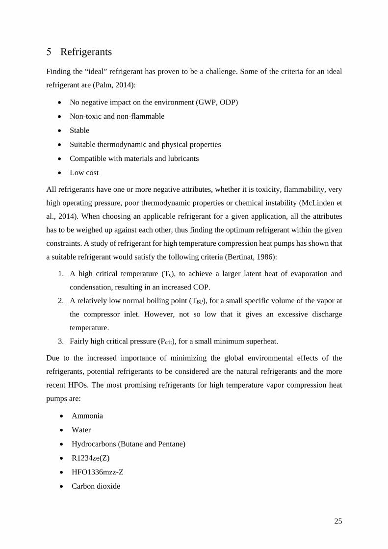
Table 5.1: Fundamental characteristics of candidate refrigerants for high temperature heat

pumps ....................................................................................................................................... 28

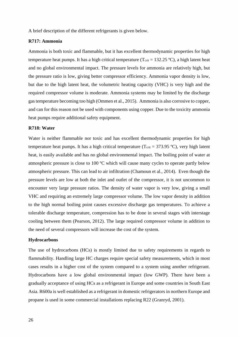
Table 5.2 Pressure loss in pipes for equal evaporator capacity ................................................ 28

Table 5.3 Pressure loss in pipes with equal mass flowrate ...................................................... 29

Table 5.4 Heat transfer coefficient ........................................................................................... 29

Table 6.1 Components for the R600 heat pump ....................................................................... 32

Table 6.2 Components for the R600a heat pump ..................................................................... 32

Table 6.3 Components for the R1234ze(Z) heat pump ............................................................ 33

Table 7.1 Evaporator inputs ..................................................................................................... 40

Table 7.2 Condenser inputs ...................................................................................................... 42

Table 7.3 Pipe dimensions for R600 ........................................................................................ 46

Table 7.4 Pipe dimensions for R600a ...................................................................................... 46

Table 7.5 Pipe dimensions for R1234ze(Z) ............................................................................. 46

Table 8.1 Inputs used in economic calculations ....................................................................... 49

Table 9.1 Chevron Angles and corresponding number of channels in evaporator .................. 61

Appendix:

Table A.1 Simulation results R600 .......................................................................................... 97

Table A.2 Simulation results R600a ........................................................................................ 98

Table A.3 Simulation results R1234ze(Z) ................................................................................ 99

Table A.4 Results for economic calculations R600 ............................................................... 100

Table A.5 Results for economic calculations R600a ............................................................. 101

Table A.6 Results for economic calculations R1234ze(Z) .................................................... 102

Table A.7 Results sensitivity analysis for R1234ze(Z) for electricity ................................... 103

Table A.8 Results sensitivity analysis for R1234ze(Z) for gas price ..................................... 104

XIV

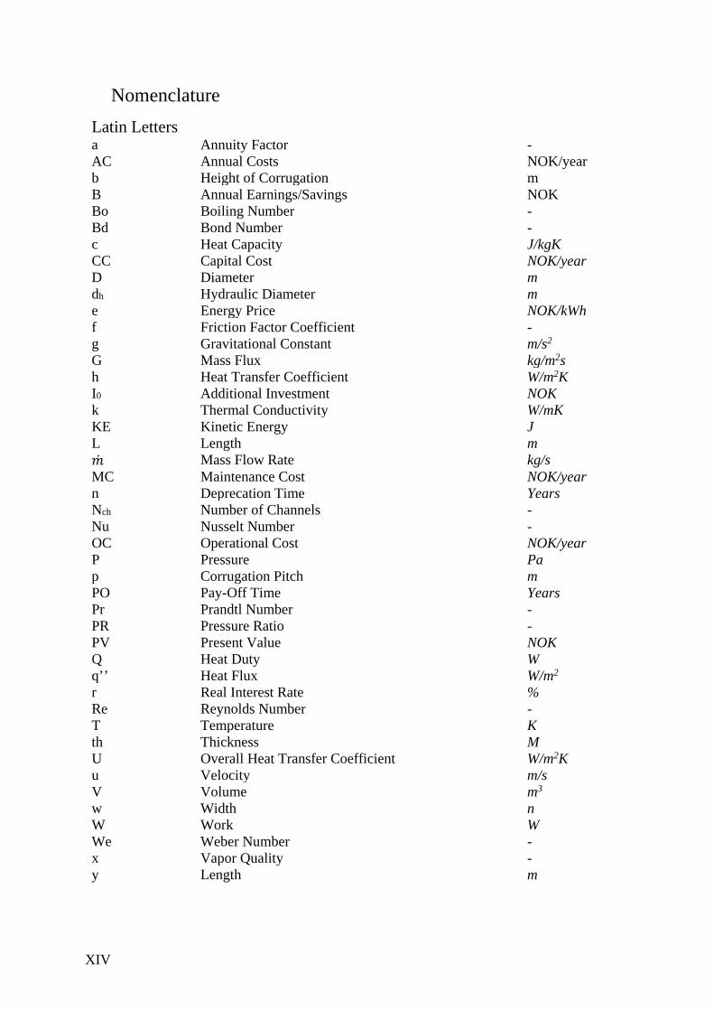
Nomenclature Latin Letters a Annuity Factor - AC Annual Costs NOK/year b Height of Corrugation m B Annual Earnings/Savings NOK Bo Boiling Number - Bd Bond Number - c Heat Capacity J/kgK CC Capital Cost NOK/year D Diameter m dh Hydraulic Diameter m e Energy Price NOK/kWh f Friction Factor Coefficient - g Gravitational Constant m/s2

G Mass Flux kg/m2s h Heat Transfer Coefficient W/m2K I0 Additional Investment NOK k Thermal Conductivity W/mK KE Kinetic Energy J L Length m �̇�𝑚 Mass Flow Rate kg/s MC Maintenance Cost NOK/year n Deprecation Time Years Nch Number of Channels - Nu Nusselt Number - OC Operational Cost NOK/year P Pressure Pa p Corrugation Pitch m PO Pay-Off Time Years Pr Prandtl Number - PR Pressure Ratio - PV Present Value NOK Q Heat Duty W q’’ Heat Flux W/m2

r Real Interest Rate % Re Reynolds Number - T Temperature K th Thickness M U Overall Heat Transfer Coefficient W/m2K u Velocity m/s V Volume m3

w Width n W Work W We Weber Number - x Vapor Quality - y Length m

XV

Greek Letters 𝛽𝛽 Chevron Angle º Δ Difference - 𝛾𝛾 Latent Heat of Vaporization J/kg 𝜂𝜂 Efficiency - 𝜇𝜇 Viscosity kg/ms 𝜌𝜌 Density kg/m3 𝜎𝜎 Surface Tension N/m 𝜆𝜆 Volumetric Efficiency - Φ Enlargement Factor -

Subscripts acc Acceleration C Cold comp Compressor cond Condenser crit Critical cross Cross Sectional eq Equivalent evap Evaporator fric Frictional g Vapor G Gravitational gas Gas Boiler H Hot HP Heat Pump is Isentropic l Liquid lo Liquid Only m Mean/Homogenous max Maximum p Port plate Heat Exchanger Plate ref Refrigerant sc Subcool sh Superheat tot Total tp Two-Phase w Water wall Plate Wall

XVI

Abbreviations BPHE Brazed Plate Heat Exchanger CAHP Compression Absorption Heat Pump CBD Conventional Batch Distillation CFC Chlorofluorocarbon COP Coefficient Of Performance EES Engineering Equation Solver GWP Global Warming Potential HC Hydrocarbons HFC Hydrofluorocarbons HFO Hydrofluoroolefin HVAC Heating, Ventilating, and Air Conditioning LMTD Logarithmic Mean Temperature Difference MVR Mechanical Vapor Recompression ODP Ozone Depletion Potential ORC Organic Rankine Cycle PHE Plate Heat Exchanger SGHE Suction Gas Heat Exchanger TVR Thermal Vapor Recompression VHC Volumetric Heating Capacity VRBD Vapor Recompressed Batch Distillation VRC Vapor Recompression

1

Introduction

Industrial waste heat often contains large amounts of useable energy that cannot be utilized in

its current form, and has to be used together with a waste heating technology to become useful.

Temperature is one of the most important factors when determining if the waste heat is useable

directly, or if it can be considered as an energy source. High temperature waste heat can often

be used directly through a heat exchanger, while low temperature waste heat has to be upgraded

(Brückner et al., 2015). Heat pumps are excellent at utilizing the energy contained in waste

heat, either by upgrading it to a usable temperature level or using it as heat source.

The heat pump technology has matured over the past two decades and heat pumps are found

increasingly in households and buildings, showing their capability and high performance. Their

use is not so widespread in the industry, due to the higher investment cost and that they are seen

as difficult and not very reliable (IEA-HPC, 2014b).

With increasing energy prices and carbon taxes, conservation and efficient use of energy will

become increasingly important in industrial operations (Chua et al., 2010). High temperature

heat pumps are capable of replacing combustion systems and electric heaters in several

applications, reducing fuel and energy consumption and in turn reducing emissions of

greenhouse gasses (Fukuda et al., 2014).

However, many of the refrigerants used in high temperature applications have had a large

negative impact on the environment. The increased focus on the environmental effects of the

refrigerants, together with stricter regulation is forcing a shift towards a generation of

refrigerants defined by a focus on global warming (Calm, 2008). Some of the potential

candidates for industrial heat pumps applications are the natural refrigerants; ammonia, carbon

dioxide, hydrocarbons, water and a new generation of synthetic refrigerants called

hydrofluoroolefins (HFOs).

When deciding for an industrial heat pumps, it is important to choose the optimal heat pump

cycle for the given scenario. To further increase the efficiency, it is important to find the optimal

operating conditions, and to reduce the losses in the system, especially for the compressors and

heat exchangers. The main goal with improving the heat pump performance is to optimize the

energy usage, making heat pumps more profitable, and as a result reduce the carbon footprint

from many energy intensive industries (Chua et al., 2010).

2

Objective

The objective of this master thesis is to investigate the potential of heat recovery from an

industrial process using heat pumps. A suitable heat pump solution is found on the basis of the

given case, where it is desired to utilize waste heat from a natural gas boiler in Lamborghinis

production facility and use it to produce hot water for washing purposes. There is a wish to

make the heat pump compact, for easier integration into an industrial plant and to use

environmentally friendly refrigerants to meet upcoming regulations. The heat pump solutions

will be evaluated based on both technical and economic feasibility.

Simulation models are developed to investigate the technical feasibility of heat pumps using

different refrigerants and to find suitable components on the market. The results are then used

to economic evaluations of the heat pump solutions and to investigate the economic feasibility

of choosing a heat pump over a competing heating solution.

Structure of the Thesis

Chapter 2 presents a short overview of different high temperature heat pump cycles and some

modifications to increase the efficiency for some of the cycles.

Chapter 3 presents a literature review of recent work and developments in the field of industrial

heat pumps. It also includes some of the recent developments done to refrigerants for industrial

heat pumps.

Chapter 4 gives a short overview of plate heat exchangers and suitable compressors.

Chapter 5 presents the criteria for suitable refrigerants for high temperature heat pumps, in

addition to giving a brief description of the different refrigerants.

Chapter 6 presents the case and the selection of suitable components.

Chapter 7 gives a description of the simulation models.

Chapter 8 gives a description of the economic model.

Chapter 9 presents the results from the simulations with an evaluating discussion.

Chapter 10 gives the conclusion.

Chapter 11 gives suggestions for further work.

3

Principle of Industrial Heat Pumps

Closed Vapor Compression Cycle

A basic closed vapor compression cycle consists of four components: an evaporator, a

compressor, a condenser and an expansion valve. A working fluid/refrigerant is circulating

inside the closed cycle. In the evaporator, the refrigerant absorbs heat from the heat source,

equal to the latent heat of vaporization (Ekroth and Granryd, 2009). The compressor compresses

the refrigerant, increasing the pressure and temperature. The refrigerant enters the condenser

where it rejects heat to the heat sink through condensation. The refrigerant returns to original

state in the evaporator by going through an expansion device, reducing the pressure and

temperature. See Figure 2.1 for a principle schematic of a cycle.

Figure 2.1 Closed vapor compression cycle

Multistage Vapor Compression Cycle

Having large temperature lifts and high-pressure ratios in heat pump systems imply lower

compression efficiencies, high discharge gas temperature out of the compressor, which may

cause degeneration of the lubricant, and high expansion losses. The main argument for having

a multistage system is to reduce the compressor losses and reduce the expansion losses (Stene,

1997). You can classify multistage vapor compression systems as either compound or cascade

systems. A compound system has two or more compression stages connected in series. See

Figure 2.2 and Figure 2.3 for two system solutions for a two-stage system.

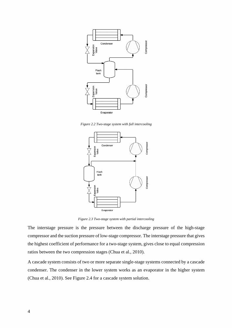
4

Figure 2.2 Two-stage system with full intercooling

Figure 2.3 Two-stage system with partial intercooling

The interstage pressure is the pressure between the discharge pressure of the high-stage

compressor and the suction pressure of low-stage compressor. The interstage pressure that gives

the highest coefficient of performance for a two-stage system, gives close to equal compression

ratios between the two compression stages (Chua et al., 2010).

A cascade system consists of two or more separate single-stage systems connected by a cascade

condenser. The condenser in the lower system works as an evaporator in the higher system

(Chua et al., 2010). See Figure 2.4 for a cascade system solution.

5

Figure 2.4 Cascade system with R1234ze(Z) and R365mfc (Kondou and Koyama, 2015).

A cascade cycle makes it possible to use different refrigerants in the different stages, making it

possible to have individual control of each stage in the cycle. The ability to choose a refrigerant

to a specific part of the cycle makes it possible to lower the operating pressure, and get good

system efficiency within the given boundaries. It is also possible to choose different piping

dimensions between the different stages and suitable lubricants for the compressors (Ekroth and

Granryd, 2009). A cascade cycle has an irreversible loss due to heat transfer in cascade

condenser. The heat transfer loss is dependent on the operating conditions and can reduce the

coefficient of performance significantly (Kondou and Koyama, 2015).

The multistage systems come at a higher investment cost compared to single stage cycles, but

the increased efficiency of the cycle will reduce the operating cost. To check if the additional

investment in a more complex system is justifiable, an economic analysis has to be performed.

Transcritical Cycles

The refrigerant in a transcritical heat pump cycle operates in both supercritical and subcritical

states. In the supercritical state, the refrigerant is a compressed gas and the temperature is

independent of the pressure. Due to this independency, heat rejection occurs at constant

pressure with a reduction in temperature. In a transcritical cycle, the condenser is therefore

exchanged for a gas cooler. Using CO2 in a transcritical cycle, has shown to be very efficient at

heating water with a large temperature difference (Nekså et al., 1998). For a CO2 transcritical

cycle an optimal gas cooler pressure exists and it depends on the operating conditions. Finding

the optimum gas cooler pressure will increase the performance of the system. This can also be

observed for other refrigerants in transcritical cycles (Sarkar et al., 2007).

6

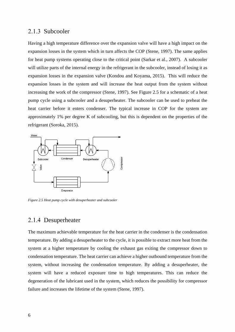
Subcooler

Having a high temperature difference over the expansion valve will have a high impact on the

expansion losses in the system which in turn affects the COP (Stene, 1997). The same applies

for heat pump systems operating close to the critical point (Sarkar et al., 2007). A subcooler

will utilize parts of the internal energy in the refrigerant in the subcooler, instead of losing it as

expansion losses in the expansion valve (Kondou and Koyama, 2015). This will reduce the

expansion losses in the system and will increase the heat output from the system without

increasing the work of the compressor (Stene, 1997). See Figure 2.5 for a schematic of a heat

pump cycle using a subcooler and a desuperheater. The subcooler can be used to preheat the

heat carrier before it enters condenser. The typical increase in COP for the system are

approximately 1% per degree K of subcooling, but this is dependent on the properties of the

refrigerant (Soroka, 2015).

Figure 2.5 Heat pump cycle with desuperheater and subcooler

Desuperheater

The maximum achievable temperature for the heat carrier in the condenser is the condensation

temperature. By adding a desuperheater to the cycle, it is possible to extract more heat from the

system at a higher temperature by cooling the exhaust gas exiting the compressor down to

condensation temperature. The heat carrier can achieve a higher outbound temperature from the

system, without increasing the condensation temperature. By adding a desuperheater, the

system will have a reduced exposure time to high temperatures. This can reduce the

degeneration of the lubricant used in the system, which reduces the possibility for compressor

failure and increases the lifetime of the system (Stene, 1997).

7

Internal Heat Exchanger

In an internal heat exchanger (suction gas heat exchanger, SGHE), heat exchange occurs

between the condensed refrigerant exiting the condenser and the gas entering the compressor

(suction gas). The condensed refrigerant is subcooled, while the suction gas is superheated. The

subcooling reduces the expansion losses in the system. Due to the superheating of the suction

gas, the exhaust gas temperature is increased which increases the superheating losses for the

system (Stene, 1997). Using an SGHE can increases the systems COP, if it is using refrigerants

with high expansion losses, like propane (R290). Ammonia on the other hand should not use a

SGHE, due to high exhaust gas temperatures. An internal heat exchanger reduces the chance

for compressor failure because it ensures superheated gas to the compressor, avoiding wet

compression (compression of droplets) (Kondou and Koyama, 2015).

8

Vapor Recompression Cycle

There are two types of vapor recompression heat pump systems (VRC). The two types are

mechanical vapor recompression (MVR) and thermal vapor recompression (TVR).

Mechanical Vapor Recompression

In many cases, low-pressure steam is rejected to the atmosphere as waste heat in energy

intensive industrial processes such as distillation and evaporation. MVR makes it possible to

recover this high quality waste heat efficiently by increasing the pressure and temperature of

the vapor (IEA-HPC, 2014a). Steam is the most common type of vapor compressed by MVR

systems but it is also possible to compress other types of waste gases (Soroka, 2015). The most

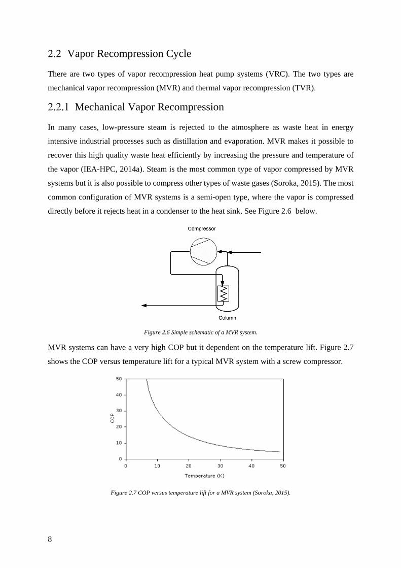
common configuration of MVR systems is a semi-open type, where the vapor is compressed

directly before it rejects heat in a condenser to the heat sink. See Figure 2.6 below.

Figure 2.6 Simple schematic of a MVR system.

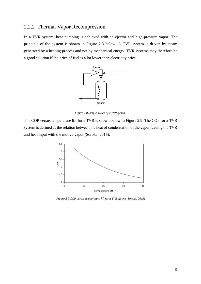
MVR systems can have a very high COP but it dependent on the temperature lift. Figure 2.7

shows the COP versus temperature lift for a typical MVR system with a screw compressor.

Figure 2.7 COP versus temperature lift for a MVR system (Soroka, 2015).

9

Thermal Vapor Recompression

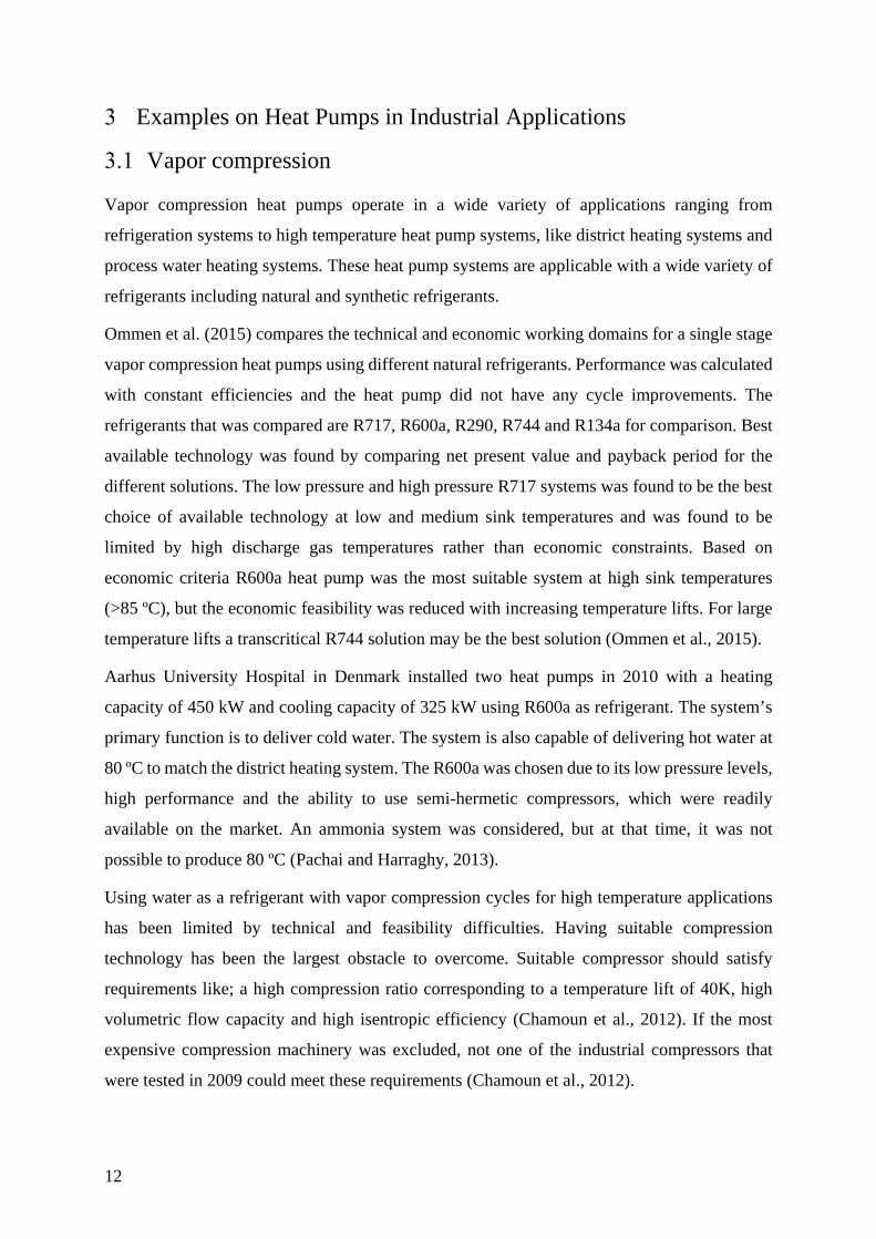
In a TVR system, heat pumping is achieved with an ejector and high-pressure vapor. The

principle of the system is shown in Figure 2.8 below. A TVR system is driven by steam

generated by a heating process and not by mechanical energy. TVR systems may therefore be

a good solution if the price of fuel is a lot lower than electricity price.

Figure 2.8 Simple sketch of a TVR system.

The COP versus temperature lift for a TVR is shown below in Figure 2.9. The COP for a TVR

system is defined as the relation between the heat of condensation of the vapor leaving the TVR

and heat input with the motive vapor (Soroka, 2015).

Figure 2.9 COP versus temperature lift for a TVR system (Soroka, 2015)

10

Absorption Heat Pump

Absorption heat pump systems distinguish themselves from the traditional heat pump systems

by being driven by heat, and not mechanical work. The absorption systems are classified as

either type I or type II. Type I is referred to as absorption heat pump and is a heat increasing

process. While type II is referred to as a heat transformer and is a temperature increasing process

(Stene, 1993). The difference between the two systems is the pressure level, and its influence

on the temperature levels, in the four main heat exchangers (evaporator, absorber,

desorber/generator and condenser) (IEA-HPC, 2014a). An absorption heat pump system is

similar to a vapor compression system; it has a condenser, an expansion system and an

evaporator. However, an absorption circuit replaces the compressor. The absorption circuit

consists of an absorber, a pump, a desorber/generator and an expansion device. See Figure 2.10

for a schematic of an absorption heat pump system. The most common mixture used in

industrial applications is a lithium bromide solution in water (LiBr/H2O) and an ammonia/water

solution (NH3/H2O) (Brückner et al., 2015). Absorption heat pumps are most suitable for

countries where electricity is generated in thermal power plants and electricity prices are high

(Stene, 1993).

Figure 2.10 Schematic of an absorption heat pump (IEA-HPC, 2014a)

11

Compression-Absorption Heat Pumps

A compression-absorption heat pump (CAHP), often called a hybrid heat pump, is based on the

mechanical vapor compression cycle. The simplest compression-absorption heat pump cycle is

the Osenbrück cycle. In the Osenbrück cycle heat transfer are performed by an absorption and

a desorption processes (Jensen et al., 2015a). A hybrid heat pump system uses a zeotropic

working fluid, which is a mixture of two or more components that will evaporate or condense

at a gliding temperature. A common zeotropic mixture used in hybrid systems are ammonia and

water (Stene, 1993). A hybrid compression-absorption system is shown in Figure 2.11 below.

Figure 2.11 Schematic diagram of a hybrid heat pump (Kim et al., 2013).

Advantages of hybrid system is the temperature glides of the absorption and desorption

processes, and a reduction of the vapor pressure, compared to the vapor pressure of a pure

working fluid (Jensen et al., 2015b). The advantage of the gliding temperature benefits the

system both in system efficiency and in an economic manner. It is economically viable if the

temperature between the heat sink and heat source is greater than 10K, when compared to a

regular vapor compression cycle. This makes the hybrid heat pump suitable for processes that

require large sink-source temperature glides (Jensen et al., 2015a). The reduction in vapor

pressure makes it possible to achieve higher supply temperatures at similar working pressures.

12

Examples on Heat Pumps in Industrial Applications

Vapor compression

Vapor compression heat pumps operate in a wide variety of applications ranging from

refrigeration systems to high temperature heat pump systems, like district heating systems and

process water heating systems. These heat pump systems are applicable with a wide variety of

refrigerants including natural and synthetic refrigerants.

Ommen et al. (2015) compares the technical and economic working domains for a single stage

vapor compression heat pumps using different natural refrigerants. Performance was calculated

with constant efficiencies and the heat pump did not have any cycle improvements. The

refrigerants that was compared are R717, R600a, R290, R744 and R134a for comparison. Best

available technology was found by comparing net present value and payback period for the

different solutions. The low pressure and high pressure R717 systems was found to be the best

choice of available technology at low and medium sink temperatures and was found to be

limited by high discharge gas temperatures rather than economic constraints. Based on

economic criteria R600a heat pump was the most suitable system at high sink temperatures

(>85 ºC), but the economic feasibility was reduced with increasing temperature lifts. For large

temperature lifts a transcritical R744 solution may be the best solution (Ommen et al., 2015).

Aarhus University Hospital in Denmark installed two heat pumps in 2010 with a heating

capacity of 450 kW and cooling capacity of 325 kW using R600a as refrigerant. The system’s

primary function is to deliver cold water. The system is also capable of delivering hot water at

80 ºC to match the district heating system. The R600a was chosen due to its low pressure levels,

high performance and the ability to use semi-hermetic compressors, which were readily

available on the market. An ammonia system was considered, but at that time, it was not

possible to produce 80 ºC (Pachai and Harraghy, 2013).

Using water as a refrigerant with vapor compression cycles for high temperature applications

has been limited by technical and feasibility difficulties. Having suitable compression

technology has been the largest obstacle to overcome. Suitable compressor should satisfy

requirements like; a high compression ratio corresponding to a temperature lift of 40K, high

volumetric flow capacity and high isentropic efficiency (Chamoun et al., 2012). If the most

expensive compression machinery was excluded, not one of the industrial compressors that

were tested in 2009 could meet these requirements (Chamoun et al., 2012).

13

A new twin screw compressor was therefore developed in the PACO project by modifying an

air compressor to meet the requirements using water vapor (Chamoun et al., 2014). The goal of

the PACO project is to develop high temperature (<140 ºC) heat pump system (700kW heating

capacity), using water as refrigerant for industrial applications. The compressor developed

should also be useful for MVR systems, used in concentration and drying applications (IEA-

HPC, 2014a).

Chamoun et al. (2014) developed a heat pump circuit for an experimental study with condensing

temperatures in the range of 130 – 140 ºC. The heat pump circuit is connected to two separate

water loops to simulate an industrial process and the use of waste heat. This system is based on

an experimental simulation of a heat recovery heat pump system for food industry done by

Assaf et al. (2010). The prototype heat pump that was developed can be seen in Figure 3.1. A

new dynamical model was also developed to take into account the non-condensable gases and

the purging mechanism related to start up procedure. The numerical simulation gave similar

results to the experimental results that were gathered. An evaluation of performance shows

good performance, but the performance is heavily dependent on the waste heat temperature and

process temperature. A short timeframe for return of investment is expected if a furnace is

replaced with this kind of heat pump (Chamoun et al., 2014). The experimental tests have shown

the technical feasibility of the system however, the expected performance is not reached, due

to mechanical problems with the screw compressor they had developed. It has now been

replaced by a centrifugal compressor and is currently in a test phase (IEA-HPC, 2014a).

Figure 3.1 Prototype heat pump with water as refrigerant (Chamoun et al., 2014).

Madsboell et al. (2015) has developed a centrifugal water vapor compressor for industrial heat

pumps in the 100-500kW range for temperature up to 110 ºC. The compressor is based on a

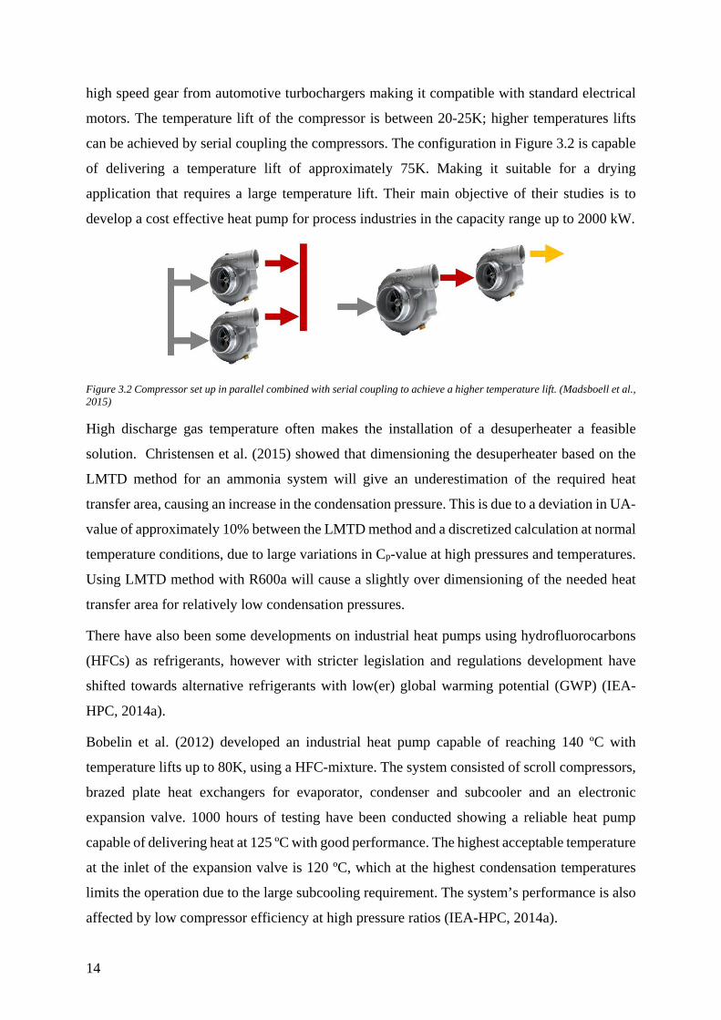
14

high speed gear from automotive turbochargers making it compatible with standard electrical

motors. The temperature lift of the compressor is between 20-25K; higher temperatures lifts

can be achieved by serial coupling the compressors. The configuration in Figure 3.2 is capable

of delivering a temperature lift of approximately 75K. Making it suitable for a drying

application that requires a large temperature lift. Their main objective of their studies is to

develop a cost effective heat pump for process industries in the capacity range up to 2000 kW.

Figure 3.2 Compressor set up in parallel combined with serial coupling to achieve a higher temperature lift. (Madsboell et al., 2015)

High discharge gas temperature often makes the installation of a desuperheater a feasible

solution. Christensen et al. (2015) showed that dimensioning the desuperheater based on the

LMTD method for an ammonia system will give an underestimation of the required heat

transfer area, causing an increase in the condensation pressure. This is due to a deviation in UA-

value of approximately 10% between the LMTD method and a discretized calculation at normal

temperature conditions, due to large variations in Cp-value at high pressures and temperatures.

Using LMTD method with R600a will cause a slightly over dimensioning of the needed heat

transfer area for relatively low condensation pressures.

There have also been some developments on industrial heat pumps using hydrofluorocarbons

(HFCs) as refrigerants, however with stricter legislation and regulations development have

shifted towards alternative refrigerants with low(er) global warming potential (GWP) (IEA-

HPC, 2014a).

Bobelin et al. (2012) developed an industrial heat pump capable of reaching 140 ºC with

temperature lifts up to 80K, using a HFC-mixture. The system consisted of scroll compressors,

brazed plate heat exchangers for evaporator, condenser and subcooler and an electronic

expansion valve. 1000 hours of testing have been conducted showing a reliable heat pump

capable of delivering heat at 125 ºC with good performance. The highest acceptable temperature

at the inlet of the expansion valve is 120 ºC, which at the highest condensation temperatures

limits the operation due to the large subcooling requirement. The system’s performance is also

affected by low compressor efficiency at high pressure ratios (IEA-HPC, 2014a).

15

The HFO R1234ze(Z), has been estimated by Brown et al. (2009) to have similar

thermodynamic properties and performance as the chlorofluorocarbon (CFC) R114. R114 was

one of the most commonly used refrigerant for high temperature heat pumps before the

Montreal Protocol (Longo et al., 2014). The estimation was based on prediction methods that

showed reasonable estimates when it was tested with R1234yf. R1234yf was the only HFO

with a more extensive data basis, than the bare minimum in open literature at the time. With no

ozone depletion potential (ODP) and the low GWP of R1234ze(Z), Brown et al. (2009)

concluded that the refrigerant deserved further considerations as to be a possible replacement

for R114 in industrial heat pumps.

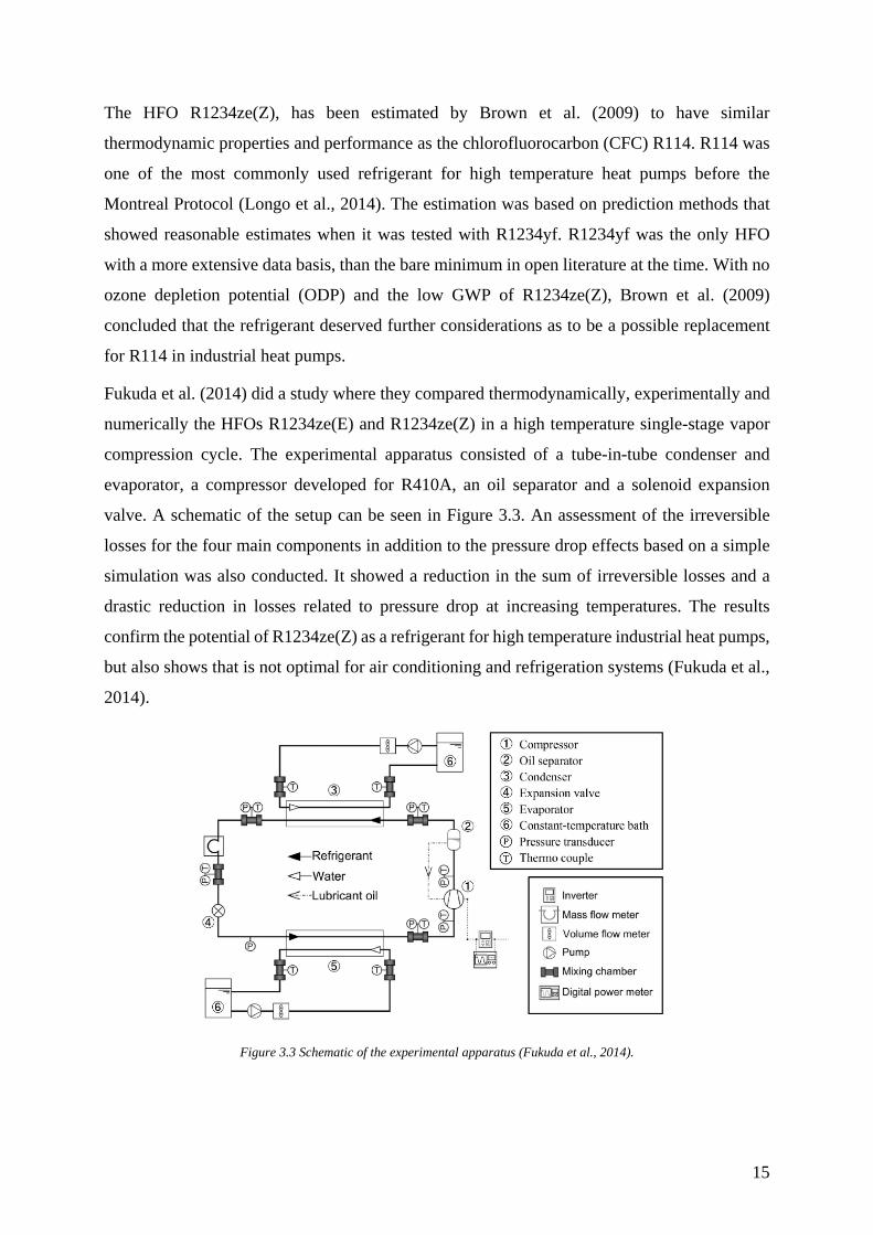
Fukuda et al. (2014) did a study where they compared thermodynamically, experimentally and

numerically the HFOs R1234ze(E) and R1234ze(Z) in a high temperature single-stage vapor

compression cycle. The experimental apparatus consisted of a tube-in-tube condenser and

evaporator, a compressor developed for R410A, an oil separator and a solenoid expansion

valve. A schematic of the setup can be seen in Figure 3.3. An assessment of the irreversible

losses for the four main components in addition to the pressure drop effects based on a simple

simulation was also conducted. It showed a reduction in the sum of irreversible losses and a

drastic reduction in losses related to pressure drop at increasing temperatures. The results

confirm the potential of R1234ze(Z) as a refrigerant for high temperature industrial heat pumps,

but also shows that is not optimal for air conditioning and refrigeration systems (Fukuda et al.,

2014).

Figure 3.3 Schematic of the experimental apparatus (Fukuda et al., 2014).

16

Taking the research a step further, Kondou and Koyama (2015) did a thermodynamic

assessment of several different heat pump cycles suitable for industrial heat recovery with the

refrigerants R717, R365mfc, R1234ze(E), and R1234ze(Z). Calculations were based on a waste

heat source of 80 ˚C producing pressurized water at 160 ˚C. The heat recovery systems were

optimized with several stages of heat extraction to reduce the throttling losses and exergy losses

in the condensers, which are connected in series. The cycles in the assessment is a triple tandem

cycle, two stage extraction cycle, three stage extraction cycle and cascade cycle. Their cascade

cycle can be seen in Figure 2.4. The systems show promising result, even at reduced heat source

temperatures. However, the effects of pressure drop are not taken into account when doing the

calculations and several of the cycles operates above their critical temperature.

Another HFO that is a potential candidate for high temperature heat pump applications is

DuPonts HFO1336mzz-Z previously known as DR-2. Kontomaris (2012) considered the

refrigerant as a low GWP alternative to R245fa. It has a high critical temperature and

thermodynamic properties making it suitable for high temperature heat pump cycles and it is

also reported to be suitable for Organic Rankine Cycles (ORC). The literature on

HFO1336mzz-Z is mainly from DuPont and Kontomaris and the discussion of this refrigerant

for high temperature applications is controversial (Fukuda et al., 2014).

Kontomaris (2016) reports that HFO1336mzz-Z is currently under laboratory and field-testing

by leading equipment manufacturers in advance of commercialization in 2017.

Transcritical Systems

Nekså et al. (1998) showed the transcritical CO2 cycle’s excellent performance at heating tap

water. Heat is rejected at constant pressure and gliding temperatures which gives an excellent

temperature fit in the gas cooler, suitable for high temperature lifts. Sarkar et al. (2004) derived

a correlation for optimum cycle parameters for a combined heating and cooling system based

on gas cooler outlet temperature and evaporator temperature. Showing the importance of an

optimum gas cooler pressure, and that the system’s COP is increased with a reduction in water

inlet temperature in the gas cooler. Transcritical CO2 cycles operate with greater pressure

differences than other refrigerants, leading to greater expansions losses. Throttling losses can

be compensated for by using ejectors, expanders or multistage expansion (Austin and Sumathy,

2011). The theoretical COP of a CO2 cycle is relatively low compared to other refrigerants, but

the actual COP of the cycle can be regarded as high, due to high compressor efficiency and

17

excellent thermodynamic properties of CO2 (Sarkar et al., 2007). In 2001, the transcritical CO2

water heater was commercialized in Japan, under the name EcoCute, as an air to water heater

capable of providing hot water at 90 ºC. Over 2 million units have been sold by 2009 (Ma et

al., 2013). Transcritical CO2 cycles are also used in refrigeration systems, district heating

systems, production of industrial process water and drying applications (IEA-HPC, 2014a).

CO2 systems are capable of delivering both hot and cold water simultaneously. A

slaughterhouse in Zürich has installed a CO2 system using waste heat from an existing ammonia

refrigeration system. The system has a total heating capacity of 800 kW at 90/30 ºC and a

refrigeration capacity of 564 kW at 20/14 ºC (IEA-HPC, 2014b). A schematic can be seen in

Figure 3.4.

The low critical temperature (31.1ºC) of CO2 limits the ability to use transcritical CO2 cycles

for waste heat recovery. If the temperature of the heat source is close to the critical point the

system will be inefficient (Kim et al., 2004).

Figure 3.4 Schematic of the CO2 heat pump in the slaughterhouse in Zürich (IEA-HPC, 2014a).

18

Compression-Absorption Heat Pumps

Hybrid heat pumps have gotten a renewed interest due to the problems finding suitable

compression heat pumps capable of high temperature lifts and temperatures, and the possibility

to use low grade waste heat for cooling (Nordtvedt, 2005). Nordtvedt (2005) experimental and

theoretical study showed the ability of the hybrid system to deliver both hot and cold water with

good performance using waste heat at 50 ºC. The experimental results showed that the capacity

could be controlled by adjusting the composition in the solution circuit. An optimum circulation

ratio and concentration of ammonia/water exists for given temperature and heating capacity.

This has to be considered carefully when designing the system (Nordtvedt, 2005, Kim et al.,

2013).

Jensen et al. (2015b) studied the technical and economic working domains of a hybrid heat

pump in comparison with vapor compression heat pumps. They showed that the hybrid heat

pump can deliver heat at temperatures up to 150 ºC, and with temperature lifts up to 60 K with

components that is commercially available. Using a hybrid heat pump was shown to be

economical beneficial over a vapor compression heat pumps when the heat supply temperature

was above 80 ºC and economically equal to ammonia vapor compression heat pumps for

condensation temperatures where they could operate.

Jensen et al. (2015a) studies the development of high temperature hybrid system using

ammonia-water. The maximum heat supply temperature is constrained by three dominating

factors; the high pressure, the compressor discharge temperature and the vapor ammonia mass

fraction. All of these constraints have to be taken into account when increasing the supply

temperature. Increasing compressions efficiency by using two-stage compression and oil

cooling is suggested to further increase the supply temperature.

Bergland et al. (2015) developed simulation models to optimize a two-stage CAHP at high

temperatures. With a maximum compressor discharge temperature of 250 ºC, it was able to

reach a maximum supply temperature of 171,8 ºC with an absorber pressure of 47,5 bar and a

COP of 2,08. A finned flat tube heat exchangers were found to be most preferable.

In Figure 3.5 there is a schematic of a hybrid heat pump with 650 kW heating capacity installed

in 2007 at a slaughterhouse, using waste heat at about 50 ºC. Average efficiency is showed to

be 4.5 over three years (Nordtvedt et al., 2013).

19

Figure 3.5 Hybrid heat pump installed at Nortura Rudshøgda (Nordtvedt et al., 2013).

Absorption Heat Pumps

The absorption systems are capable of providing cooling and heating. Absorption chillers can

be integrated in plants where there is a demand for cooling and there is waste heat available.

The most efficient working fluid for absorption system is a water/lithium bromide mixture

(Oluleye et al., 2016). However, they cannot operate below 0 ºC, so for lower temperatures an

ammonia/water mixture is used. Absorption chillers can also be used in district cooling systems.

The COP of the system is dependent on the temperature of the heat source, higher temperatures

gives higher COP (Broberg Viklund and Johansson, 2014).

Qu and Abdelaziz (2015) simulated the use of an absorption heat pump integrated into a coal

power plant. The results suggested that the size of the cooling towers and the water usage could

be reduced by 17%, reducing the construction and the operational costs. In addition to the

reducing the cooling demand of the towers, the absorption heat pump would also produce hot

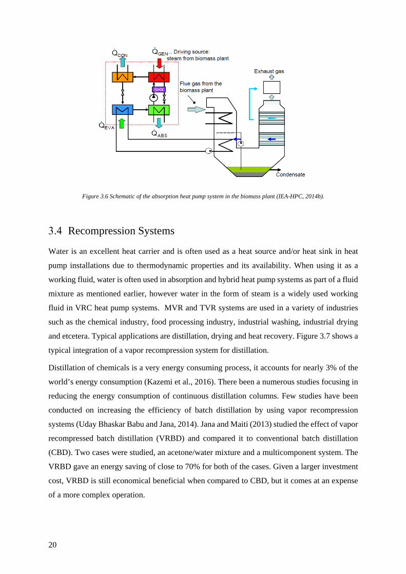
water. Schweighofer Fibre GmbH in Austria has installed a single-stage absorption heat pump

in their biomass power plant. A schematic of the installation can be seen in Figure 3.6. It

subcools the flue gas in the evaporator, making it possible to use its condensation heat. Steam

from the biomass plant is used to drive the generator in the system. The delivered heat from the

system is used in a district heating network (IEA-HPC, 2014b).

20

Figure 3.6 Schematic of the absorption heat pump system in the biomass plant (IEA-HPC, 2014b).

Recompression Systems

Water is an excellent heat carrier and is often used as a heat source and/or heat sink in heat

pump installations due to thermodynamic properties and its availability. When using it as a

working fluid, water is often used in absorption and hybrid heat pump systems as part of a fluid

mixture as mentioned earlier, however water in the form of steam is a widely used working

fluid in VRC heat pump systems. MVR and TVR systems are used in a variety of industries

such as the chemical industry, food processing industry, industrial washing, industrial drying

and etcetera. Typical applications are distillation, drying and heat recovery. Figure 3.7 shows a

typical integration of a vapor recompression system for distillation.

Distillation of chemicals is a very energy consuming process, it accounts for nearly 3% of the

world’s energy consumption (Kazemi et al., 2016). There been a numerous studies focusing in

reducing the energy consumption of continuous distillation columns. Few studies have been

conducted on increasing the efficiency of batch distillation by using vapor recompression

systems (Uday Bhaskar Babu and Jana, 2014). Jana and Maiti (2013) studied the effect of vapor

recompressed batch distillation (VRBD) and compared it to conventional batch distillation

(CBD). Two cases were studied, an acetone/water mixture and a multicomponent system. The

VRBD gave an energy saving of close to 70% for both of the cases. Given a larger investment

cost, VRBD is still economical beneficial when compared to CBD, but it comes at an expense

of a more complex operation.

21

Operational experience from IEA HPP ANNEX 35 has shown that standardized MVR systems

used in the different industries are reliable, can have a high reduction in primary energy usage

which in turn reduces costs and gives a short payback time, especially if the systems are

installed in new built plants (IEA-HPC, 2014b).

Figure 3.7 Typical vapor recompression distillation process flow sheet (Kazemi et al., 2016).

22

Components

Plate Heat Exchangers

Plate heat exchangers (PHEs) are a wildly used industrial applications, such as heating,

refrigeration, air-conditioning (HVAC), chemical processing, etc. They have a high heat

transfer efficiency and a large heat transfer surface area per volume, giving a reduced refrigerant

charge compared to other type of heat exchangers. A smaller refrigerant charge gives a reduced

environmental impact and lowers the inventory cost (Eldeeb et al., 2016). The 4 most

commonly used PHEs are: gasketed plate heat exchangers, brazed plate heat exchangers

(BPHEs), welded and semi-welded heat exchangers and shell and plate heat exchangers (Amalfi

et al., 2016a). The PHEs are highly flexible; it is possible to specify the amount of plates to get

the wanted performance (Shah and Sekulić, 2007). On the gasketed plate heat exchanger it is

possible to add or remove plates if there is need for a higher or lower heat output. The plates

used in the different heat exchangers are often made of stainless steel. BPHEs consists of several

plates brazed together, most commonly by copper or nickel, which allows them to operate under

high pressure and temperature conditions. They are highly compact and have a reduced chance

of leakage in addition to offering high heat duties. Making them suitable for process water

heating and heat recovery (Eldeeb et al., 2016). A schematic with relevant parameters for a

plate used in PHEs can be seen in Figure 4.1.

Figure 4.1 Schematic view of a plate (Longo, 2010)

An important parameter when doing calculations on PHEs is the hydraulic diameter 𝑑𝑑ℎ, it is

defined as (Martin, 1996):

𝑑𝑑ℎ =2𝑏𝑏Φ

( 4.1 )

23

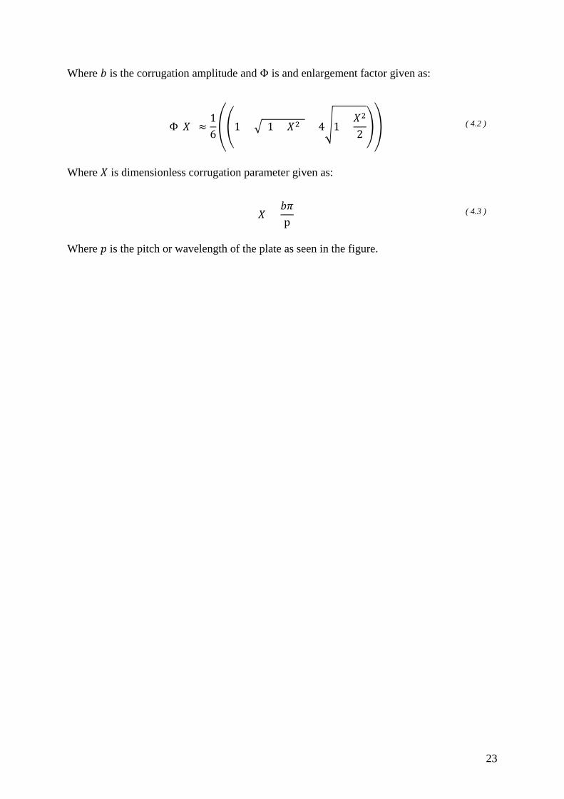
Where 𝑏𝑏 is the corrugation amplitude and Φ is and enlargement factor given as:

Φ(𝑋𝑋) ≈16��

1 + �(1 + 𝑋𝑋2) + 4�1 +𝑋𝑋2

2 �� ( 4.2 )

Where 𝑋𝑋 is dimensionless corrugation parameter given as:

𝑋𝑋 =𝑏𝑏𝑏𝑏p

( 4.3 )

Where 𝑝𝑝 is the pitch or wavelength of the plate as seen in the figure.

24

Compressors

The compressor types that is most used in industrial size applications are reciprocating

compressors, screw compressors and turbo compressor. The compressors handle different

displacement ranges where the reciprocating compressor handles the smallest compressor

volumes while turbo compressors can handle the largest, with the screw compressor in the

intermediate range (Eikevik et al., 2016). To find a suitable compressor the required compressor

volume in 𝑚𝑚3

ℎ is calculated in ( 4.4 ):

𝑉𝑉�̇�𝑠 =�̇�𝑚𝜌𝜌𝑔𝑔 𝜆𝜆 ∗ 3600 ( 4.4 )

𝜆𝜆 is the volumetric efficiency, �̇�𝑚 is the mass flow rate of the refrigerant and 𝜌𝜌𝑔𝑔 is the gas density

at inlet of the compressor.

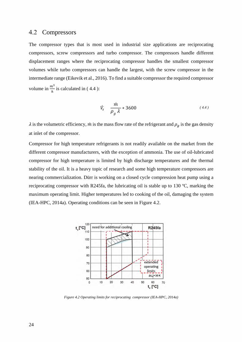
Compressor for high temperature refrigerants is not readily available on the market from the

different compressor manufacturers, with the exception of ammonia. The use of oil-lubricated

compressor for high temperature is limited by high discharge temperatures and the thermal

stability of the oil. It is a heavy topic of research and some high temperature compressors are

nearing commercialization. Dürr is working on a closed cycle compression heat pump using a

reciprocating compressor with R245fa, the lubricating oil is stable up to 130 ºC, marking the

maximum operating limit. Higher temperatures led to cooking of the oil, damaging the system

(IEA-HPC, 2014a). Operating conditions can be seen in Figure 4.2.

Figure 4.2 Operating limits for reciprocating compressor (IEA-HPC, 2014a)

25

Refrigerants

Finding the “ideal” refrigerant has proven to be a challenge. Some of the criteria for an ideal

refrigerant are (Palm, 2014):

• No negative impact on the environment (GWP, ODP)

• Non-toxic and non-flammable

• Stable

• Suitable thermodynamic and physical properties

• Compatible with materials and lubricants

• Low cost

All refrigerants have one or more negative attributes, whether it is toxicity, flammability, very

high operating pressure, poor thermodynamic properties or chemical instability (McLinden et

al., 2014). When choosing an applicable refrigerant for a given application, all the attributes

has to be weighed up against each other, thus finding the optimum refrigerant within the given

constraints. A study of refrigerant for high temperature compression heat pumps has shown that

a suitable refrigerant would satisfy the following criteria (Bertinat, 1986):

1. A high critical temperature (Tc), to achieve a larger latent heat of evaporation and

condensation, resulting in an increased COP.

2. A relatively low normal boiling point (TBP), for a small specific volume of the vapor at

the compressor inlet. However, not so low that it gives an excessive discharge

temperature.

3. Fairly high critical pressure (Pcrit), for a small minimum superheat.

Due to the increased importance of minimizing the global environmental effects of the

refrigerants, potential refrigerants to be considered are the natural refrigerants and the more

recent HFOs. The most promising refrigerants for high temperature vapor compression heat

pumps are:

• Ammonia

• Water

• Hydrocarbons (Butane and Pentane)

• R1234ze(Z)

• HFO1336mzz-Z

• Carbon dioxide

26

A brief description of the different refrigerants is given below.

R717: Ammonia

Ammonia is both toxic and flammable, but it has excellent thermodynamic properties for high

temperature heat pumps. It has a high critical temperature (Tcrit = 132.25 ºC), a high latent heat

and no global environmental impact. The pressure levels for ammonia are relatively high, but

the pressure ratio is low, giving better compressor efficiency. Ammonia vapor density is low,

but due to the high latent heat, the volumetric heating capacity (VHC) is very high and the

required compressor volume is moderate. Ammonia systems may be limited by the discharge

gas temperature becoming too high (Ommen et al., 2015). Ammonia is also corrosive to copper,

and can for this reason not be used with components using copper. Due to the toxicity ammonia

heat pumps require additional safety equipment.

R718: Water

Water is neither flammable nor toxic and has excellent thermodynamic properties for high

temperature heat pumps. It has a high critical temperature (Tcrit = 373.95 ºC), very high latent

heat, is easily available and has no global environmental impact. The boiling point of water at

atmospheric pressure is close to 100 ºC which will cause many cycles to operate partly below

atmospheric pressure. This can lead to air infiltration (Chamoun et al., 2014). Even though the

pressure levels are low at both the inlet and outlet of the compressor, it is not uncommon to

encounter very large pressure ratios. The density of water vapor is very low, giving a small

VHC and requiring an extremely large compressor volume. The low vapor density in addition

to the high normal boiling point causes excessive discharge gas temperatures. To achieve a

tolerable discharge temperature, compression has to be done in several stages with interstage

cooling between them (Pearson, 2012). The large required compressor volume in addition to

the need of several compressors will increase the cost of the system.

Hydrocarbons

The use of hydrocarbons (HCs) is mostly limited due to safety requirements in regards to

flammability. Handling large HC charges require special safety measurements, which in most

cases results in a higher cost of the system compared to a system using another refrigerant.

Hydrocarbons have a low global environmental impact (low GWP). There have been a

gradually acceptance of using HCs as a refrigerant in Europe and some countries in South East

Asia. R600a is well established as a refrigerant in domestic refrigerators in northern Europe and

propane is used in some commercial installations replacing R22 (Granryd, 2001).

27

The hydrocarbons of interest for high temperature applications are Butane and Pentane. Both

n-butane (R600) and isobutane (R600a) have similar performance to each other at low

temperature conditions while the cycle performance of R600 is better in high temperature

conditions. The discharge temperature for R600 is also shown to be lower at similar conditions

(Pan et al., 2011). R600 has a high critical temperature (Tcrit=151.98 ºC) and moderate operating

pressures. R600a on the other hand has a critical temperature of (Tcrit=134,66 ºC) and moderate

operating pressure, but slightly higher than R600. R601 has a higher critical temperature

(Tcrit=196.55 ºC) and even lower operating pressures. Both refrigerants have low discharge gas

temperature, and need some superheating at high temperatures to avoid liquid compression.

R1234ze(Z)

R1234ze(Z) is a newer synthetic refrigerant in the HFO family. It has a high critical temperature

(Tcrit=150.1 ºC), moderate operating pressures and a low environmental effect (low GWP). It is

regarded a promising refrigerant with similar potential capabilities as the CFC, R114 (Longo et

al., 2014). It is expected to be mildly flammable (Kondou and Koyama, 2015). An experimental

study comparing properties of R1234ze(Z) in a commercial brazed plate heat exchanger

(BPHE) against commonly used HFCs and HCs showed a much higher heat transfer coefficient

and a frictional pressure drop similar to R600a (Longo et al., 2014). See chapter 3.1 for recent

developments.

HFO1336mzz-Z

A new HFO from DuPont, it is previously known as DR-2. It is not yet commercially available.

It has a high critical temperature (Tcrit=171.3 ºC), it is expected to be non-toxic and non-

flammable and a low environmental effect (low GWP). See chapter 3.1 for recent

developments.

R744: Carbon dioxide

CO2 has a relatively low critical temperature (Tcrit=31.1 ºC), which makes CO2 heat pump cycle

operate above the critical point, in a supercritical phase. Heat is rejected at constant pressure

and gliding temperatures and not through condensation. Transcritical CO2 cycles operate at

very high pressure (Pearson, 2012). The pressure levels for CO2 are very high, but the pressure

ratio is low, giving high compressor efficiency. CO2 also have a very high vapor density giving

a small required compressor volume and very compact compressors. CO2 is environmentally

friendly and is neither toxic nor flammable. The gliding temperature and the excellent

thermodynamic properties of CO2 make it excellent at heating water when the temperature lift

28

is large. As stated in 3.1.1 the use of CO2 for industrial heat pumps using waste heat is limited

by high temperatures of the heat source.

Table 5.1 lists currently used and potential candidates for high temperature heat pumps using

waste heat as its heat source. R114 is listed as a reference for comparison.

Table 5.1: Fundamental characteristics of candidate refrigerants for high temperature heat pumps

Name R114 R717 R718 R600 R600a R601 R1234ze(Z) HFO1336mzz-Z

Formula C2Cl2F4 NH3 H20 C4H10 C4H10 C5H12 CHF=CHCF3(Z) CF3CH=CHCF3(Z) Molar mass (kg/kmol) 170,92 17,03 18,02 58,12 58,12 72,15 114,00a 164,06b

ODP 0,8e 0 0 0 0 0 0a 0b GWP100 9800c 0 0 20d 20d 20d <1a 2b

Safety A1c B2 A1 A3 A3 A3 A2La A1b

NBP (°C) 3,59 -33,33 99,97 -0,49 -11,75 36,06 9,80a 33,40b Pc (bar) 32,57 113,33 220,64 37,96 36,29 33,70 35,30a 29,00b

Tcrit (°C) 145,68 132,25 373,95 151,98 134,66 196,55 150,10a 171,30b

Data from REFPROP 9.0 (Lemmon et al.) with the expectations of: a (Kondou and Koyama, 2015) b (Kontomaris, 2014) c (Longo et al., 2014) d (Pan et al., 2011) e (Devotta and Rao Pendyala, 1994)

Pressure Loss in Pipes

The pressure drop for a selection of the refrigerants is given in Table 5.2. The values are

calculated using EES inbuilt function Pipeflow (Klein, 2015) for an ideal heat pump with an

evaporator capacity of 150 kW. The refrigerant has an evaporation temperature of 40 ºC with

no superheat and a condensation temperature of 80 ºC. The pressure drop in Table 5.2 is

calculated at the exit of the evaporator. The pipe has diameter of 0,05 m, length of 5 m and a

roughness of 0,15 mm equal to commercial galvanized steel pipes (Nellis and Klein, 2009).

Table 5.2 Pressure loss in pipes for equal evaporator capacity

Name R114 R717 R600 R600a R601 R1234ze(Z)

Δ𝑃𝑃 [𝑃𝑃𝑃𝑃] 51860 838,2 14651 13914 35791 26480

�̇�𝑚𝑟𝑟𝑟𝑟𝑟𝑟 [𝑘𝑘𝑔𝑔𝑠𝑠

] 1,896 0,168 0,6252 0,7331 0,5855 1,03

29

In Table 5.3 the pressure loss is calculated using the same mass flow rate.

Table 5.3 Pressure loss in pipes with equal mass flowrate

Name R114 R717 R600 R600a R601 R1234ze(Z)

Δ𝑃𝑃 [𝑃𝑃𝑃𝑃] 14448 29388 37440 25870 104305 24957

�̇�𝑚𝑟𝑟𝑟𝑟𝑟𝑟 [𝑘𝑘𝑔𝑔𝑠𝑠

] 1,00 1,00 1,00 1,00 1,00 1,00

Film Condensation on a Vertical Plate

The heat transfer coefficients are calculated for the different refrigerants using EES inbuilt

function Cond_Vertical_Plate (Klein, 2015). With a plate length of 1 m, width of 0,5 m, wall

temperature of 80 ºC and a saturation temperature of the fluid of 85 ºC. This function calculates

the heat transfer coefficient on the basis of a general correlation based on the Reynolds number.

The validity of these values are uncertain, but they can be used to give a perspective on how

the heat transfer coefficient of the different fluids compare to each other. Longo et al. (2014)

measurements in brazed plate heat exchangers suggests that R1234ze(Z) should have higher

heat transfer coefficients than R600a. Cavallini et al. (2006) suggests that R600 has higher heat

transfer coefficients is larger than R600a in horizontal tubes. Table 5.4 suggest similar results.

Table 5.4 Heat transfer coefficient

Name R114 R717 R600 R600a R601 R1234ze(Z)

h �𝑊𝑊𝑚𝑚2𝐾𝐾

� 633,8 4557 1140 976,6 1236 1031

30

Case

The Lamborghini automobile manufacturing plant in Sant’ Agata Bolognese is vertical

integrated, including the production of carbon fiber used in the car manufacturing. The carbon

fiber autoclaves are heated by natural gas fired oil boilers. The flue gas that is produced, has a

temperature of 200ºC, where 30% of the energy corresponds to sensible heat that can be

recovered by an economizer. The remaining energy is latent heat contained in the water vapor

generated by the natural gas burning which is released at condensation at approximately 60 ºC.

The factory has a need for 90 ºC hot water for washing purposes.

A heat pump solution should be able to recover heat from the carbon fiber production process

and use it to cover the hot water demand. An economic and technical evaluation is conducted

to investigate; if investing in heat pump solution is favorable over an investment in a natural

gas boiler.

A schematic of the plant with an integrated heat pump circuit can be seen in Figure 6.1.

Figure 6.1 Schematic of the plant

Operating Conditions

The operating time of the heat pump is assumed to be 4400 hours a year, which corresponds to

approximately 12 hours a day. The amount of water needed to be heated in the condenser is set

to 10 kg/s and the mass flow rate in the evaporator is set to be 7 kg/s. The required heat duty is

approximately 210 kW, which equals to a yearly energy consumption of 924 000 kWh.

31

The base evaporation and condensation temperature is set to 40 ºC and 100 ºC respectively. The

evaporation temperature is varied between 40 ºC and 44 ºC while the condensation temperature

is kept constant and the evaporation temperature is kept constant when the condensation

temperature is varied between 100 ºC and 92 ºC.

Choosing Suitable Components

A single-stage vapor compression heat pump using R600, R600a and R1234ze(Z) was chosen

for the model. This was chosen over a two-stage heat pump due to a low pressure ratio (would

be around 2 for the selected refrigerants), only a small increase in energy saving based on

simplified calculations, the low discharge superheat for R600 and R600a which could result in

liquid compression without sufficient superheating and the fact that is desireable to have a

compact system.

Out of the suitable low GWP refrigerants R600a, R600 and R1234ze(Z) was chosen for the

simulations mainly due to the lack of suitable heat transfer coeffeicent correlations for the other

refrigerants. They are also the refrigerants expected to have the highest performance and be the

most suitable for the given boundaries based on the literature that was reviewed.

The components were chosen on the basis of R600 and R600a for high temperature applications

and they are assumed to be working with R1234ze(Z) due to the similarities in pressure drop

and heat transfer.

The different heat exchangers were chosen by using SWEP’s calculation software with inputs

given by the simulation model (SWEP, 2016). This resulted in the same evaporator and

condenser but different amount of plates in SGHE for R600 and R600a. R1234ze(Z) do not

need a SGHE, and it’s therefor removed from the calculations.

The compressors series were chosen based on the supplier’s calculation tools for R600 and

R600a (Johnson Controls Norway, 2016). Their capacity was assumed to be equal to their

capacity at 1500 rpm. This assumption is however not correct, since the chosen compressor

series had to run at 1000 RPM with R600a, resulting in a larger compressor for R600a than for

R600. Which would result in a higher compressor cost for R600a than for R600. The prices for

the two smallest compressors was extrapolated basis on the prices given for two larger

compressors.

The expansion valve was selected by using Danfoss’ selection software for R600a and

R600 (Danfoss, 2016). The controller and sensors was then selected on the basis of the

expansion valve.

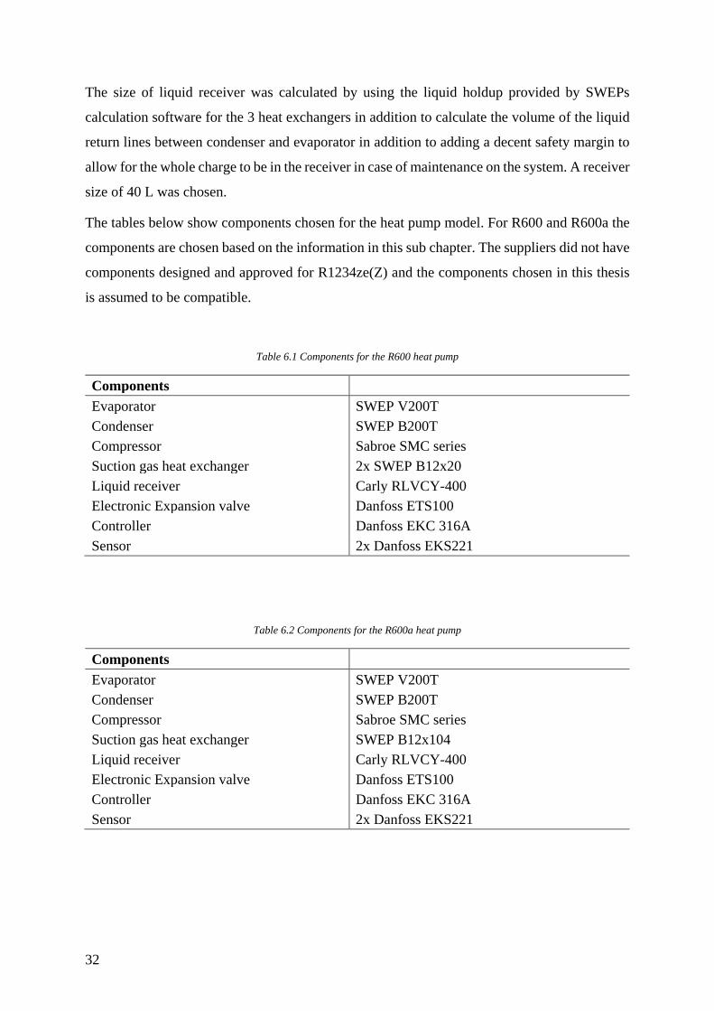
32

The size of liquid receiver was calculated by using the liquid holdup provided by SWEPs

calculation software for the 3 heat exchangers in addition to calculate the volume of the liquid

return lines between condenser and evaporator in addition to adding a decent safety margin to

allow for the whole charge to be in the receiver in case of maintenance on the system. A receiver

size of 40 L was chosen.

The tables below show components chosen for the heat pump model. For R600 and R600a the

components are chosen based on the information in this sub chapter. The suppliers did not have

components designed and approved for R1234ze(Z) and the components chosen in this thesis

is assumed to be compatible.

Table 6.1 Components for the R600 heat pump

Components Evaporator SWEP V200T Condenser SWEP B200T Compressor Sabroe SMC series Suction gas heat exchanger 2x SWEP B12x20 Liquid receiver Carly RLVCY-400 Electronic Expansion valve Danfoss ETS100 Controller Danfoss EKC 316A Sensor 2x Danfoss EKS221

Table 6.2 Components for the R600a heat pump

Components Evaporator SWEP V200T Condenser SWEP B200T Compressor Sabroe SMC series Suction gas heat exchanger SWEP B12x104 Liquid receiver Carly RLVCY-400 Electronic Expansion valve Danfoss ETS100 Controller Danfoss EKC 316A Sensor 2x Danfoss EKS221

33

Table 6.3 Components for the R1234ze(Z) heat pump

Components Evaporator SWEP V200T Condenser SWEP B200T Compressor Sabroe SMC series Liquid receiver Carly RLVCY-400 Electronic Expansion valve Danfoss ETS100 Controller Danfoss EKC 316A Sensor 2x Danfoss EKS221

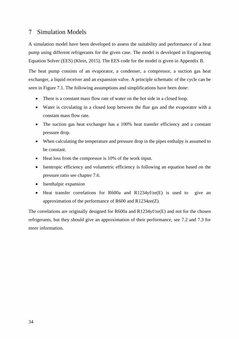
34

Simulation Models

A simulation model have been developed to assess the suitability and performance of a heat

pump using different refrigerants for the given case. The model is developed in Engineering

Equation Solver (EES) (Klein, 2015). The EES code for the model is given in Appendix B.

The heat pump consists of an evaporator, a condenser, a compressor, a suction gas heat

exchanger, a liquid receiver and an expansion valve. A principle schematic of the cycle can be

seen in Figure 7.1. The following assumptions and simplifications have been done:

• There is a constant mass flow rate of water on the hot side in a closed loop.

• Water is circulating in a closed loop between the flue gas and the evaporator with a

constant mass flow rate.

• The suction gas heat exchanger has a 100% heat transfer efficiency and a constant

pressure drop.

• When calculating the temperature and pressure drop in the pipes enthalpy is assumed to

be constant.

• Heat loss from the compressor is 10% of the work input.

• Isentropic efficiency and volumetric efficiency is following an equation based on the

pressure ratio see chapter 7.6.

• Isenthalpic expansion

• Heat transfer correlations for R600a and R1234yf/ze(E) is used to give an

approximation of the performance of R600 and R1234ze(Z).

The correlations are originally designed for R600a and R1234yf/ze(E) and not for the chosen

refrigerants, but they should give an approximation of their performance, see 7.2 and 7.3 for

more information.

35

Figure 7.1 Schematic of the heat pump model

36

Heat Exchangers

The heat exchangers are modeled with a numerical procedure to find the heat exchanger area

and heat transfer needed to meet the required heat duties. The heat exchanger is divided into

small control volumes and an energy balance is conducted. The step size for the calculations is

chosen to be 3 𝑚𝑚 and there are 300 integration step equaling to a control volume length of

0,01 𝑚𝑚. The state equations are derived from Nellis and Klein (2009) for a parallel flow plate

heat exchanger. The state equation used to calculate the change in water temperature per length

in the evaporator can be seen in ( 7.1 ) and the condenser in ( 7.2 ):

𝑑𝑑𝑇𝑇𝐻𝐻𝑑𝑑𝑑𝑑

= −2 𝑁𝑁𝑐𝑐ℎ(𝑇𝑇𝐻𝐻 − 𝑇𝑇𝐶𝐶)

�̇�𝑚ℎ𝑐𝑐𝐻𝐻 �1

ℎ𝐻𝐻𝑤𝑤+ 𝑡𝑡ℎ𝑚𝑚𝑘𝑘𝑚𝑚𝑤𝑤

+ 1ℎ𝐶𝐶𝑤𝑤

� ( 7.1 )

𝑑𝑑𝑇𝑇𝐶𝐶𝑑𝑑𝑑𝑑

=2 𝑁𝑁𝑐𝑐ℎ(𝑇𝑇𝐻𝐻 − 𝑇𝑇𝐶𝐶)

�̇�𝑚𝐶𝐶𝑐𝑐𝐶𝐶 �1

ℎ𝐻𝐻𝑤𝑤+ 𝑡𝑡ℎ𝑚𝑚𝑘𝑘𝑚𝑚𝑤𝑤

+ 1ℎ𝐶𝐶𝑤𝑤

� ( 7.2 )

Where 𝑁𝑁𝑐𝑐ℎ is the number of channels in the heat exchanger, 𝑇𝑇ℎ and 𝑇𝑇𝑐𝑐 is the temperature for

the hot and cold fluid, �̇�𝑚 is the mass flow rate hot or cold fluid, 𝑐𝑐 is the heat capacity of the

fluid, ℎ is the heat transfer coefficient for the hot and cold fluids, 𝑤𝑤 is the width of the heat

exchanger, 𝑡𝑡ℎ𝑚𝑚 is the thickness of the plate and 𝑘𝑘𝑚𝑚 is the metal conductivity at the local average

temperature.

The change in temperature is used to calculate the enthalpy change, which in turn gives the heat

transferred to or from the refrigerant. The next control volume is calculated on the basis of

values of the previous control volume, this procedure will go on until the desired outlet

conditions are met. The temperature change in the refrigerant is given by the saturation pressure.

The saturation pressure is affected by a pressure drop in the heat exchanger leading to a

temperature fall.

To be able to calculate the state equations, the heat transfer coefficients for the refrigerant and

water has to be found. Several heat transfer coefficients and frictional pressure drop correlations

are available for plate heat exchangers in the literature. These correlations are found from

experimental setups and are valid within a certain range of operating conditions, defined by i.e.

Reynolds number, mass flux, temperatures among others. The correlations that are available is

made for temperatures and refrigerants used in typical refrigeration and heat pump applications

and not for high temperature heat pumps and for “newer” refrigerants. The correlations used in

the model will therefore not give accurate representation of real heat exchangers but a useful

37

approximation, due to the similarities of the refrigerants. More information about the separate

heat exchangers and the correlations can be found in chapter 7.2 and 7.3.

Summaries of correlations for plate heat exchangers is available in (García-Cascales et al.,

2007), (Eldeeb et al., 2016) and (Amalfi et al., 2016a).

Evaporator

Heat is transferred from the warmer water to the refrigerant in the evaporator, cooling the water

while increasing the enthalpy and thus the vapor quality of refrigerant. The refrigerant will go

through a transition from a two-phase flow at the inlet to a single-phase flow at the outlet of the

evaporator. The two-phase heat transfer coefficient is modeled with Amalfi et al. (2016b)

correlation for flow boiling in plate heat exchangers. This correlation is valid for a vapor quality

between 0 < 𝑑𝑑 < 0,90. The correlation is based on dimensional analysis developed from 1903

heat transfer data points for a wide range of operating conditions, geometries and fluids. The

Nusselt is given by:

𝑁𝑁𝑢𝑢𝑡𝑡𝑡𝑡 = �982 𝛽𝛽∗1,101 𝑊𝑊𝑊𝑊𝑚𝑚

0,315𝐵𝐵𝐵𝐵0,320𝜌𝜌∗−0,224 ,𝐵𝐵𝑑𝑑 < 418,495 𝛽𝛽∗0,248𝑅𝑅𝑊𝑊𝑣𝑣

0,135𝑅𝑅𝑊𝑊𝑙𝑙𝑙𝑙0,351𝐵𝐵𝑑𝑑0,235𝐵𝐵𝐵𝐵0,198𝜌𝜌∗−0,223,𝐵𝐵𝑑𝑑 ≥ 4

( 7.3 )

Bond number less than 4 represents microscale geometries and macroscale for Bond number

greater than or equal to 4. The Bond number is defined as:

𝐵𝐵𝑑𝑑 =(𝜌𝜌𝑙𝑙 − 𝜌𝜌𝑣𝑣)𝑔𝑔𝑑𝑑ℎ2

𝜎𝜎 ( 7.4 )

Where 𝑑𝑑ℎ is the hydraulic diameter, 𝜌𝜌𝑙𝑙 is the liquid density, 𝜌𝜌𝑣𝑣 is the vapor density and 𝑔𝑔 is the

gravitational constant. The density ratio 𝜌𝜌∗ is defined as:

𝜌𝜌∗ =𝜌𝜌𝑙𝑙𝜌𝜌𝑣𝑣

( 7.5 )

𝛽𝛽∗ takes the chevron angle into account and is defined as:

𝛽𝛽∗ =𝛽𝛽

𝛽𝛽𝑚𝑚𝑚𝑚𝑚𝑚 ( 7.6 )

Where 𝛽𝛽𝑚𝑚𝑚𝑚𝑚𝑚 = 70°. The homogeneous Weber number 𝑊𝑊𝑊𝑊𝑚𝑚 is defined as:

38

𝑊𝑊𝑊𝑊𝑚𝑚 =𝐺𝐺2𝑑𝑑ℎ𝜌𝜌𝑚𝑚𝜎𝜎

( 7.7 )

Where 𝜎𝜎 is the surface tension, 𝐺𝐺 is the mass flux and 𝜌𝜌𝑚𝑚 is the homogenous density:

𝜌𝜌𝑚𝑚 =1

𝑑𝑑𝑚𝑚𝜌𝜌𝑣𝑣

+ 1 − 𝑑𝑑𝑚𝑚𝜌𝜌𝑙𝑙

( 7.8 )

𝐺𝐺 =�̇�𝑚

𝐴𝐴𝑐𝑐𝑟𝑟𝑙𝑙𝑠𝑠𝑠𝑠𝑁𝑁𝑐𝑐ℎ ( 7.9 )

𝑑𝑑𝑚𝑚 is the mean vapor fraction and 𝐴𝐴𝑐𝑐𝑟𝑟𝑙𝑙𝑠𝑠𝑠𝑠 is the cross dimensional area. The boiling number 𝐵𝐵𝐵𝐵

is defined as:

𝐵𝐵𝐵𝐵 =𝑞𝑞′′

𝐺𝐺𝛾𝛾 ( 7.10 )

𝑞𝑞′′ is the heat flux and 𝛾𝛾 is the latent heat of vaporization. The Reynolds number for vapor, 𝑅𝑅𝑊𝑊𝑣𝑣

is defined as:

𝑅𝑅𝑊𝑊𝑣𝑣 =𝐺𝐺𝑑𝑑𝑑𝑑ℎ𝜇𝜇𝑣𝑣

( 7.11 )

Where 𝑑𝑑 is the vapor fraction and 𝜇𝜇𝑣𝑣 is the dynamic viscosity for vapor phase. The Reynolds

number for a liquid flow, 𝑅𝑅𝑊𝑊𝑙𝑙𝑙𝑙 is defined as:

𝑅𝑅𝑊𝑊𝑙𝑙𝑙𝑙 =𝐺𝐺𝑑𝑑ℎ𝜇𝜇𝑙𝑙

( 7.12 )

Where 𝜇𝜇𝑙𝑙 is the dynamic viscosity for the liquid phase. The Nusselt number is used to calculate

the heat transfer for the two-phase flow:

ℎ𝑡𝑡𝑡𝑡 =𝑁𝑁𝑢𝑢𝑡𝑡𝑡𝑡 𝑘𝑘𝑙𝑙𝑑𝑑ℎ

( 7.13 )

Where 𝑘𝑘𝑙𝑙 is the conductivity for the liquid phase.

39

When the vapor quality is between 0,90 < 𝑑𝑑 < 1 the heat transfer coefficient will decrease

linearly down to 600 𝑊𝑊𝑚𝑚2𝐾𝐾

(Eikevik, 2016). When 𝑑𝑑 = 1 the heat transfer coefficient for the

refrigerant is found using the Martin correlation for single-phase flow in a plate heat exchanger

(García-Cascales et al., 2007). The Nusselt number is given by:

𝑁𝑁𝑢𝑢 = 0,122𝑃𝑃𝑃𝑃13 �

𝜇𝜇𝜇𝜇𝑤𝑤𝑚𝑚𝑙𝑙𝑙𝑙

�16 (𝑓𝑓𝑅𝑅𝑊𝑊2 sin(2𝛽𝛽))0,374 ( 7.14 )

Where 𝜇𝜇 is the viscosity for the fluid, 𝜇𝜇𝑤𝑤𝑚𝑚𝑙𝑙𝑙𝑙 is the viscosity at the wall and the friction factor 𝑓𝑓

is given by:

1�𝑓𝑓

=cos𝛽𝛽

�0,18 tan𝛽𝛽 + 0,36 sin𝛽𝛽 + 𝑓𝑓𝑙𝑙cos𝛽𝛽�

1/2 +1 − cos𝛽𝛽�3,8 𝑓𝑓1

( 7.15 )

and 𝑓𝑓0 and 𝑓𝑓1 is defined by the Reynolds number:

𝑓𝑓𝑙𝑙 = �64𝑅𝑅𝑊𝑊

, 𝑅𝑅𝑊𝑊 < 2000

(1,8 log10 𝑅𝑅𝑊𝑊 − 1,5)−2 , 𝑅𝑅𝑊𝑊 ≥ 2000 ( 7.16 )

𝑓𝑓1 = �

597𝑅𝑅𝑊𝑊

+ 3,85 , 𝑅𝑅𝑊𝑊 < 2000

39𝑅𝑅𝑊𝑊0,289 , 𝑅𝑅𝑊𝑊 ≥ 2000

( 7.17 )

The Nusselt number is used to calculate the heat transfer coefficient:

ℎ =𝑁𝑁𝑢𝑢 𝑘𝑘𝑑𝑑ℎ

( 7.18 )

The heat transfer coefficient for the water in the evaporator is found using the Martin correlation

for single-phase flow in a plate heat exchanger.

Frictional Pressure Drop

The frictional pressure drop in the evaporator caused by the refrigerant is predicted using two-

phase friction factor coefficient for plate heat exchangers from Amalfi et al. (2016b). The

friction factor is based on 1513 pressure drop data points and can be predicted as follows:

40

𝑓𝑓𝑡𝑡𝑡𝑡 = 𝐶𝐶 ∗ 15,698 𝑊𝑊𝑊𝑊𝑚𝑚−0,475𝐵𝐵𝑑𝑑0,255𝜌𝜌∗−0,571 ( 7.19 )

Where the C parameter takes the effect of the corrugation angle into consideration:

𝐶𝐶 = 2,125 𝛽𝛽∗9,993 + 0,955 ( 7.20 )

When the refrigerant is being superheated the friction factor is calculated using ( 7.15 ). The

friction factor is used to calculate the frictional pressure drop at each step(Δ𝑦𝑦) in the evaporator:

Δ𝑃𝑃𝑟𝑟𝑟𝑟𝑓𝑓𝑐𝑐 =2 𝑓𝑓 𝐺𝐺2Δ𝑦𝑦𝑑𝑑ℎ ∗ 𝜌𝜌𝑚𝑚

( 7.21 )

The inputs for the evaporator is given in Table 7.1. The length and width is based on the chosen

brazed plate heat exchanger. The height and pitch of the corrugation and chevron angle is taken

from (Longo et al., 2015a). The thickness of the plates is chosen based on typical values for

BPHE (Wang et al., 2007). The plate thickness needs to be able to withstand the pressure level

in the heat exchanger. Maximum number of plates are 250 equal to 125 channels.

Table 7.1 Evaporator inputs

Inputs Value Length 𝐿𝐿 0,450 [m] Width 𝑊𝑊 0,243 [m] Number of channels 𝑁𝑁𝑐𝑐ℎ Variable [-] Maximum number of channels 𝑁𝑁𝑐𝑐ℎ;𝑚𝑚𝑚𝑚𝑚𝑚 125 [-] Corrugation pitch 𝑝𝑝 0,008 [m] Height of the corrugation 𝑏𝑏 0,002 [m] Hydraulic diameter 𝑑𝑑ℎ 0,0035 [m] Chevron angle 𝛽𝛽 45 [deg] Thickness of plate 𝑇𝑇ℎ𝑚𝑚 0,0005 [m] Superheat 𝑇𝑇𝑠𝑠ℎ 5 [K]

41

Condenser

In the condenser heat is transferred from the refrigerant to the water, heating the water while

decreasing the enthalpy and thus the vapor quality of refrigerant. The refrigerant will go through

a transition from a superheated single-phase flow at the inlet to a subcooled single-phase flow

at the outlet of the condenser by going through a two-phase region with condensation. The

superheated and subcooled region are calculated using the Martin correlation for single-phase

flow. The two-phase heat transfer coefficient is modeled with Longo et al. (2015b) correlation

for condensation in plate heat exchangers. The correlation is based on and compared against an

experimental data set covering a range of operating conditions, geometries and fluids. The heat

transfer coefficient is giving by:

ℎ𝑠𝑠𝑚𝑚𝑡𝑡 = 1,875 Φ�𝑘𝑘𝑙𝑙𝑑𝑑ℎ�𝑅𝑅𝑊𝑊𝑟𝑟𝑒𝑒

0,445𝑃𝑃𝑃𝑃𝑙𝑙1/3 ( 7.22 )

Where Φ is an enlargement factor, 𝑃𝑃𝑃𝑃𝑙𝑙 is the liquid Prandtl number and 𝑅𝑅𝑊𝑊𝑟𝑟𝑒𝑒 is the equivalent

Reynolds number given by:

𝑅𝑅𝑊𝑊𝑟𝑟𝑒𝑒 =𝐺𝐺𝑟𝑟𝑒𝑒𝑑𝑑ℎ𝜇𝜇𝑙𝑙

( 7.23 )

Where the equivalent mass flux is:

𝐺𝐺𝑟𝑟𝑒𝑒 = 𝐺𝐺 �(1 − 𝑑𝑑𝑚𝑚) + 𝑑𝑑𝑚𝑚 �𝜌𝜌𝑙𝑙𝜌𝜌𝑔𝑔�1/2

� ( 7.24 )

The heat transfer coefficient for the water in the condenser is found using the Martin correlation

for single-phase flow in a plate heat exchanger.

Frictional Pressure Drop

The frictional pressure drop in the condenser is predicted using a linear equation based on the

kinetic energy per unit volume from Longo (2010). The equation is based on experimental data

with hydrocarbons in BPHE:

Δ𝑃𝑃𝑟𝑟𝑟𝑟𝑓𝑓𝑐𝑐 = 1,90𝐾𝐾𝐾𝐾𝑉𝑉

( 7.25 )

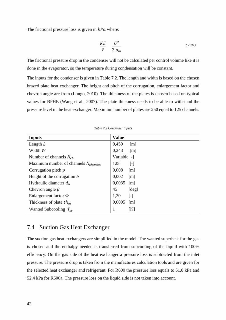
42

The frictional pressure loss is given in 𝑘𝑘𝑃𝑃𝑃𝑃 where:

𝐾𝐾𝐾𝐾𝑉𝑉

=𝐺𝐺2

2 𝜌𝜌𝑚𝑚 ( 7.26 )

The frictional pressure drop in the condenser will not be calculated per control volume like it is

done in the evaporator, so the temperature during condensation will be constant.

The inputs for the condenser is given in Table 7.2. The length and width is based on the chosen

brazed plate heat exchanger. The height and pitch of the corrugation, enlargement factor and

chevron angle are from (Longo, 2010). The thickness of the plates is chosen based on typical

values for BPHE (Wang et al., 2007). The plate thickness needs to be able to withstand the

pressure level in the heat exchanger. Maximum number of plates are 250 equal to 125 channels.

Table 7.2 Condenser inputs

Inputs Value Length 𝐿𝐿 0,450 [m] Width 𝑊𝑊 0,243 [m] Number of channels 𝑁𝑁𝑐𝑐ℎ Variable [-] Maximum number of channels 𝑁𝑁𝑐𝑐ℎ;𝑚𝑚𝑚𝑚𝑚𝑚 125 [-] Corrugation pitch 𝑝𝑝 0,008 [m] Height of the corrugation 𝑏𝑏 0,002 [m] Hydraulic diameter 𝑑𝑑ℎ 0,0035 [m] Chevron angle 𝛽𝛽 45 [deg] Enlargement factor Φ 1,20 [-] Thickness of plate 𝑡𝑡ℎ𝑚𝑚 0,0005 [m] Wanted Subcooling 𝑇𝑇𝑠𝑠𝑐𝑐 1 [K]

Suction Gas Heat Exchanger

The suction gas heat exchangers are simplified in the model. The wanted superheat for the gas

is chosen and the enthalpy needed is transferred from subcooling of the liquid with 100%

efficiency. On the gas side of the heat exchanger a pressure loss is subtracted from the inlet

pressure. The pressure drop is taken from the manufactures calculation tools and are given for

the selected heat exchanger and refrigerant. For R600 the pressure loss equals to 51,8 kPa and

52,4 kPa for R600a. The pressure loss on the liquid side is not taken into account.

43

Pressure Loss in the Heat Exchangers

The measured pressure drop in the heat exchangers consists of several components. The total

pressure drop in the evaporator is calculated by (Amalfi et al., 2016a):

Δ𝑃𝑃𝑡𝑡𝑙𝑙𝑡𝑡,𝑟𝑟𝑣𝑣𝑚𝑚𝑡𝑡 = Δ𝑃𝑃𝐺𝐺 + Δ𝑃𝑃𝑚𝑚𝑐𝑐𝑐𝑐 + Δ𝑃𝑃𝑟𝑟𝑟𝑟𝑓𝑓𝑐𝑐 + Δ𝑃𝑃𝑡𝑡 ( 7.27 )

And the total pressure drop in the condenser (Longo, 2010):

Δ𝑝𝑝𝑡𝑡𝑙𝑙𝑡𝑡,𝑐𝑐𝑙𝑙𝑐𝑐𝑐𝑐 = −Δ𝑃𝑃𝐺𝐺 − Δ𝑃𝑃𝑚𝑚𝑐𝑐𝑐𝑐 + Δ𝑃𝑃𝑟𝑟𝑟𝑟𝑓𝑓𝑐𝑐 + Δ𝑃𝑃𝑡𝑡 ( 7.28 )

Where Δ𝑃𝑃𝐺𝐺 is the pressure loss due to gravity, Δ𝑃𝑃𝑚𝑚𝑐𝑐𝑐𝑐 is pressure loss due to acceleration(or

deceleration), Δ𝑃𝑃𝑡𝑡 is pressure loss across the inlet and outlet ports in addition to the frictional

pressure loss Δ𝑃𝑃𝑟𝑟𝑟𝑟𝑓𝑓𝑐𝑐 which is calculated in ( 7.21 ) and ( 7.25 ). The Δ𝑃𝑃𝐺𝐺 is negative in the

condenser because it’s chosen that the refrigerant flows downwards, increasing the pressure. In

the condenser the refrigerant decelerate when it is transitioning from gas to liquid, increasing

the pressure. The different components are defined by:

Δ𝑃𝑃𝐺𝐺 = 𝜌𝜌𝑚𝑚 𝑔𝑔 𝐿𝐿𝑡𝑡𝑙𝑙𝑚𝑚𝑡𝑡𝑟𝑟 ( 7.29 )

Δ𝑃𝑃𝑚𝑚𝑐𝑐𝑐𝑐 = 𝐺𝐺2Δ𝑑𝑑 �1𝜌𝜌𝑔𝑔

−1𝜌𝜌𝑙𝑙� ( 7.30 )

Δ𝑃𝑃𝑡𝑡 = 0,75 𝑁𝑁𝑡𝑡𝑚𝑚𝑠𝑠𝑠𝑠 � �𝐺𝐺𝑝𝑝2

2𝜌𝜌�𝑓𝑓𝑐𝑐

+ �𝐺𝐺𝑝𝑝2

2𝜌𝜌�𝑙𝑙𝑜𝑜𝑡𝑡

� ( 7.31 )

Where 𝐿𝐿𝑡𝑡𝑙𝑙𝑚𝑚𝑡𝑡𝑟𝑟 is the length of the plate. The number of passes 𝑁𝑁𝑡𝑡𝑚𝑚𝑠𝑠𝑠𝑠 is chosen to be 1 in the

model.

44

Compressor

The compressor work is calculated using isentropic efficiency and a heat loss. The isentropic

efficiency is calculated using ( 7.32 ) using the pressure ratio (Eikevik et al., 2016). The formula

is based on measurements done on a piston compressor, it is not measured on the chosen

compressors for this system. However, it does take the change in efficiency based on pressure

ratio into account, instead of using a constant efficiency for all pressure ratios. The heat loss is

constant and equal to 10% of the compressor work.

𝜂𝜂𝑓𝑓𝑠𝑠 = −0,00000461 𝑃𝑃𝑅𝑅6 + 0,00027131 𝑃𝑃𝑅𝑅5 − 0,00628605 𝑃𝑃𝑅𝑅4 + 0,07370258 𝑃𝑃𝑅𝑅3− 0,46054399 𝑃𝑃𝑅𝑅2 + 1,40653347 𝑃𝑃𝑅𝑅 − 0,87811477

( 7.32 )

The volumetric efficiency is calculated using ( 7.33 ), which is made from the same

measurements.

λ = 0,0011 𝑃𝑃𝑅𝑅2 − 0,0487 𝑃𝑃𝑅𝑅 + 0,9979 ( 7.33 )

45

Piping

The piping is used to connect the different components in the system. While the refrigerant is

flowing through the pipes a pressure loss will occur due to friction between the pipe wall and

the fluid, which in turn increases the work needed to be done by the compressor. This pressure

loss is calculated by calling the built in function 𝑃𝑃𝑃𝑃𝑝𝑝𝑊𝑊𝑓𝑓𝑃𝑃𝐵𝐵𝑤𝑤 (Klein, 2015). It returns the pressure

drop for a given mass flow rate through a circular tube with a given length and diameter. The

pressure drop is used to find the temperature fall by assuming that the flow has a constant

enthalpy.

Another important aspect to take into account when designing the system is having sufficient

flow velocity in the pipes, this is to ensure sufficient oil return. An insufficient oil return is one

of the most important practical problems that needs to be solved when designing a heat pump

system. Choosing an oil that can withstand the required temperatures, that mixes good with the

refrigerant and that gives a sufficient oil return is important if the system should operate

properly over several years. Insufficient oil return can result in oil holdup in the heat

exchangers, especially in the evaporator, reducing the heat transfer. When the oil is not reaching

the compressor to lubricate it and to remove heat, the result could be overheating or damage to

the compressor.

To have a sufficient transportation of oil in vertical pipes Bäckström (1946) suggested that:

𝜌𝜌𝑔𝑔𝑢𝑢𝑔𝑔2 ≥ 126 ( 7.34 )

𝑢𝑢𝑔𝑔 is gas velocity. For the liquid return lines a sufficient flow velocity would be 𝑢𝑢𝑙𝑙 > 0,5 𝑚𝑚/𝑠𝑠

(Eikevik, 2016).

The Norwegian Refrigeration and Heat Pump Norm recommends 9 − 10 𝑚𝑚/𝑠𝑠 in the suction

pipeline, 6 − 7 𝑚𝑚/𝑠𝑠 in the pressure pipeline and 5 𝑚𝑚/𝑠𝑠 in the return pipeline (Haukås, 2015).

This values are meant to give efficient oil return and moderate pressure/temperature loss in

pipelines.

On the basis of the suggested flow velocities, diameters for the pipes have been chosen. The

length and diameter of the different pipes can be found in Table 7.3, Table 7.4 and Table 7.5.

This results in velocities around 9 − 10 𝑚𝑚/𝑠𝑠 in the suction line, 6 − 7 𝑚𝑚/𝑠𝑠 in the pressure

pipeline and 2 − 3,5 𝑚𝑚/𝑠𝑠 in the return lines for the 3 systems. Which should give a sufficient

oil return. The roughness is chosen to be 0,15 𝑚𝑚𝑚𝑚, this is equal to commercial galvanized steel

pipes (Nellis and Klein, 2009).

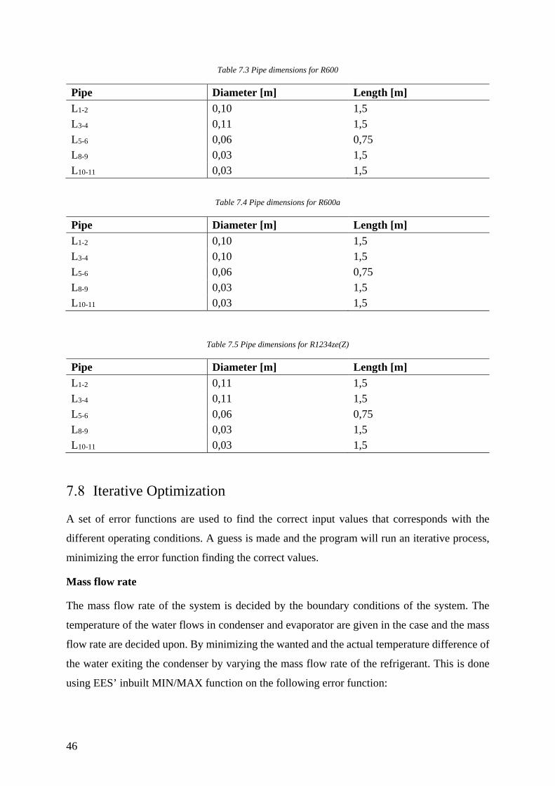
46

Table 7.3 Pipe dimensions for R600

Pipe Diameter [m] Length [m] L1-2 0,10 1,5 L3-4 0,11 1,5 L5-6 0,06 0,75 L8-9 0,03 1,5 L10-11 0,03 1,5

Table 7.4 Pipe dimensions for R600a


Table 7.5 Pipe dimensions for R1234ze(Z)


Iterative Optimization

A set of error functions are used to find the correct input values that corresponds with the

different operating conditions. A guess is made and the program will run an iterative process,

minimizing the error function finding the correct values.

Mass flow rate

The mass flow rate of the system is decided by the boundary conditions of the system. The

temperature of the water flows in condenser and evaporator are given in the case and the mass

flow rate are decided upon. By minimizing the wanted and the actual temperature difference of

the water exiting the condenser by varying the mass flow rate of the refrigerant. This is done

using EES’ inbuilt MIN/MAX function on the following error function:

47

errtemp;cond = abs(Tw;real;out − Twater;out;cond) ( 7.35 )

This function is used for the different fluids at 𝑇𝑇𝑟𝑟 = 40 °𝐶𝐶 and 𝑇𝑇𝑐𝑐 = 100 °𝐶𝐶 and the mass flow

rate is then kept constant for other operating conditions. It will cause a slight deviation for the

water temperatures in heat exchangers but it is done to keep operating conditions similar for the

3 systems.

Condensation pressure

Due to a pressure drop in the pipe between the compressor exit and the condenser inlet an error

function is made to account for the loss. It is done by guessing the pressure drop in the pipe and

adding this to the compressor outlet pressure:

Pguess;comp = X [Pa] ( 7.36 )

𝑃𝑃𝑙𝑙𝑜𝑜𝑡𝑡;𝑐𝑐𝑙𝑙𝑚𝑚𝑡𝑡 = 𝑃𝑃𝑟𝑟𝑟𝑟𝑟𝑟;𝑐𝑐𝑙𝑙𝑐𝑐𝑐𝑐 + 𝑃𝑃𝑔𝑔𝑜𝑜𝑟𝑟𝑠𝑠𝑠𝑠;𝑐𝑐𝑙𝑙𝑚𝑚𝑡𝑡 ( 7.37 )

The error function is then minimized using MIN/MAX:

𝑊𝑊𝑃𝑃𝑃𝑃𝑐𝑐𝑙𝑙𝑚𝑚𝑡𝑡 = 𝑃𝑃𝑏𝑏𝑠𝑠(𝑃𝑃𝑔𝑔𝑜𝑜𝑟𝑟𝑠𝑠𝑠𝑠;𝑐𝑐𝑙𝑙𝑚𝑚𝑡𝑡 − Δ𝑃𝑃56) ( 7.38 )

Where Δ𝑃𝑃56 is the pressure drop in the pipe between the compressor and evaporator.

Number of Plates in Evaporator and Condenser

The number of plates used in the heat exchangers is decided by two error functions that

compares the calculated length of the heat exchanger versus the length of the plates. If it is not

possible to get the exact length the number of plates is increased so the length out of the heat

exchangers is shorter than the plate. This is done by varying the number of channels in the heat

exchangers. The error functions used is:

𝑊𝑊𝑃𝑃𝑃𝑃𝑙𝑙𝑟𝑟𝑐𝑐𝑔𝑔𝑡𝑡ℎ;𝑐𝑐𝑙𝑙𝑐𝑐𝑐𝑐 = 𝑃𝑃𝑏𝑏𝑠𝑠(𝐿𝐿𝑡𝑡𝑙𝑙𝑚𝑚𝑡𝑡𝑟𝑟;𝑐𝑐𝑙𝑙𝑐𝑐𝑐𝑐 − 𝐿𝐿𝑙𝑙𝑜𝑜𝑡𝑡;𝑐𝑐𝑙𝑙𝑐𝑐𝑐𝑐) ( 7.39 )

𝑊𝑊𝑃𝑃𝑃𝑃𝑙𝑙𝑟𝑟𝑐𝑐𝑔𝑔𝑡𝑡ℎ;𝑟𝑟𝑣𝑣𝑚𝑚𝑡𝑡 = 𝑃𝑃𝑏𝑏𝑠𝑠(𝐿𝐿𝑡𝑡𝑙𝑙𝑚𝑚𝑡𝑡𝑟𝑟;𝑟𝑟𝑣𝑣𝑚𝑚𝑡𝑡 − 𝐿𝐿𝑙𝑙𝑜𝑜𝑡𝑡;𝑟𝑟𝑣𝑣𝑚𝑚𝑡𝑡) ( 7.40 )

48

Economic model

An economic model has been created to compare the operational and investment costs of the

different heat pump solutions in addition to comparing them with a traditional heating solution,

namely a natural gas boiler. The annual cost for the different solutions is calculated by summing

the annual capital cost, the annual operational cost and the annual maintenance cost as shown

in ( 8.1 ):

𝐴𝐴𝐶𝐶 = �(𝐼𝐼0 𝑃𝑃)𝑐𝑐 + �(𝑊𝑊𝑟𝑟 𝑊𝑊) + �𝑀𝑀𝐶𝐶 ( 8.1 )

Where 𝐼𝐼0 is the additional investment cost for each subsystem, 𝑃𝑃 is the annuity factor, 𝑊𝑊𝑟𝑟 is the

energy demand, 𝑊𝑊 is the energy price and 𝑀𝑀𝐶𝐶 is the maintenance costs. The maintenance cost

is calculated as a percentage of the investment cost. The annuity factor is calculated by:

𝑃𝑃 =𝑃𝑃

1 − (1 + 𝑃𝑃)−𝑐𝑐 ( 8.2 )

Where 𝑃𝑃 is the real interest rate and 𝑛𝑛 is the depreciation time.

To assess if it is profitable to invest in the different heat pump solutions over a natural gas boiler

a profitability analysis is conducted. This is done using the Present Value Method and Pay-Off

Time (Stene, 2016). The Present Value Method shows the absolute profitability of an

investment. If a heat pump project has a 𝑃𝑃𝑉𝑉 > 0 then its regarded as a profitable investment.

PV is calculated by:

𝑃𝑃𝑉𝑉 =𝐵𝐵𝑃𝑃− 𝐼𝐼0 ( 8.3 )

Where 𝐵𝐵 is the net annual earnings/saving and 𝐼𝐼0 is the additional investment cost compared to

competing heating systems. 𝐵𝐵 gives the annual cost reduction for operation and maintenance

compared to other heating solutions. 𝐵𝐵 is calculated by:

𝐵𝐵 = (𝑃𝑃𝑛𝑛𝑛𝑛𝑢𝑢𝑃𝑃𝑃𝑃 𝑠𝑠𝑃𝑃𝑠𝑠𝑃𝑃𝑛𝑛𝑔𝑔𝑠𝑠 − 𝑃𝑃𝑛𝑛𝑛𝑛𝑢𝑢𝑃𝑃𝑃𝑃 𝑐𝑐𝐵𝐵𝑠𝑠𝑡𝑡𝑠𝑠) ( 8.4 )

49

Pay-Off Time will result in the number of years it takes before the sum of net annual savings

equals to the additional investment cost, while taking account the real interest rate. This makes

the method more accurate than “Pay-Back Time”. Pay-off time is calculated by:

𝑃𝑃𝑃𝑃=𝑃𝑃𝑛𝑛 ��1 − �𝐼𝐼0𝐵𝐵� 𝑃𝑃�

−1�

𝑃𝑃𝑛𝑛(1 + 𝑃𝑃) ( 8.5 )

In addition to this the specific heating cost is calculated:

𝑆𝑆𝑆𝑆𝐶𝐶 = (𝐴𝐴𝐶𝐶𝑄𝑄ℎ

) ( 8.6 )

The specific heating cost does not say anything about the profitability of the investment, but

will give the cost per kWh.

Lastly a sensitivity analysis is conducted by varying the electricity prices and natural gas prices.

The electricity and natural gas prices was based on the average prices for the second half of

2013 in member countries of the European Union. The prices for natural gas was 0,04

Euro/kWh and 0,118 Euro/kWh for electricity (Eurostat, 2016). An exchange rate of 1 Euro

equal to 9,3 NOK was used in the calculations. Resulting in a price of 0,37 NOK/kWh for

natural gas and 1,10 NOK/kWh for electricity. Inputs can be seen in Table 8.1.

Table 8.1 Inputs used in economic calculations

Inputs Value Real interest rate 𝑃𝑃 5 [%] Depreciation time 𝑛𝑛 25 [years] Running time 4400 [hours] Heat Duty 𝑄𝑄 210 [kW] Energy demand 924 000 [kWh] Annual maintenance cost heat pump 6 [%] Annual maintenance cost gas boiler 3 [%] Efficiency gas boiler η𝑔𝑔𝑚𝑚𝑠𝑠 0,95 [-] Gas price egas 0,37 [NOK/kWh] Electricity price eel 1,10 [NOK/kWh]

50

Simulation Results

The effect of varying the operating conditions for the 3 heat pump cycles is assessed in the

following chapter. The condensation temperature was kept constant while the evaporation

temperature was varied, and opposite when the evaporation temperature was kept constant and

condensation temperature was varied. The mass flow rate was also kept constant for all

operating condition. This was done to reduce the degrees of freedom, easing the process of

finding the amount of plates and operating pressure for the given conditions. This will also

highlight the effect of the individual parameter.

The results were then used to do economic evaluations for the different systems, including

finding a suitable compressor and calculate the total investment cost and operating cost. This

was then used to do investment analysis for the different solutions comparing them against a

natural gas boiler.

51

The Effect of Changing the Evaporation Temperature

The effect on the systems COP by varying the evaporation temperature is seen in Figure 9.1.

The condensation temperature was kept at 100 ºC. The system using R1234ze(Z) has the highest

COP, and by increasing the evaporation temperature the COP increases from 3 to 3,8. The COP

for R600 and R600a is lower mainly due to an additional pressure drop of approximately 50

kPa in the suction gas heat exchanger due to the need for additional superheating. Increasing

the evaporation temperature still have a beneficial effect, increasing the COP to 3,5 for R600

and 3,4 for R600a from 2,8.

Figure 9.1 COP vs evaporation temperature

One of the main reasons for the increase in COP is the reduction of pressure drop in the

evaporator. The pressure drop is plotted against the evaporation temperature in Figure 9.2. The

reduction of pressure drop in the evaporator has several beneficial consequences; it reduces the

pressure ratio for the system, increasing the compressors isentropic and volumetric efficiency

in addition to reducing the required work need to be done by the compressor. It also reduces

the required compressor volume at the compressor inlet due to increase vapor density. This

reduces the required size of the compressor, potentially decreasing the investment cost. As seen

in the figure, R1234ze(Z) have the highest overall pressure drop of the refrigerants, but the

difference will be reduced at increasing temperatures. R600a show similar pressure drops to

R1234ze(Z) but slightly lower overall. R600 have the lowest pressure drops, especially at 40

ºC but the difference is smaller at 44 ºC. When comparing the pressure drop Figure 9.2 with

the corresponding number of channels in Figure 9.3, an significant reduction in pressure drop

2,5

2,7

2,9

3,1

3,3

3,5

3,7

3,9

40 41 42 43 44

CO

P

Evaporation Temperature [ºC]

R600 R600a R1234ze(Z)

52

can be observed by a relatively small increase in heat exchanger channels. R1234ze(Z) requires

the most channels, while R600a requires the fewest.

Figure 9.2 Pressure drop in evaporator at different evaporation temperatures

Figure 9.3 Number of channels required in the evaporator for different evaporation temperatures

10000

20000

30000

40000

50000

60000

70000

80000

40 41 42 43 44

Pres

sure

Dro

p [P

a]


R600 R600a R1234ze(Z)

0

5

10

15

20

25

30

35

40

40 41 42 43 44

Num

ber

of C

hann

els [

-]


R600 R600a R1234ze(Z)

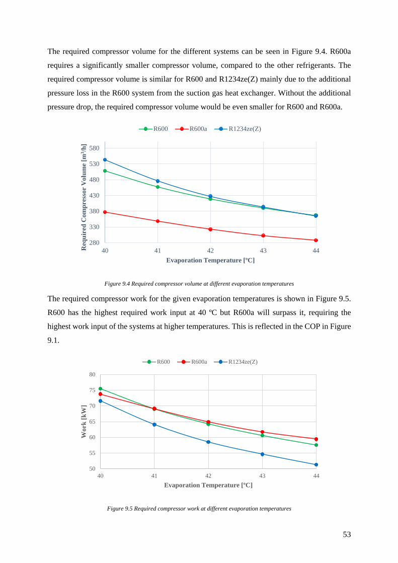
53

The required compressor volume for the different systems can be seen in Figure 9.4. R600a

requires a significantly smaller compressor volume, compared to the other refrigerants. The

required compressor volume is similar for R600 and R1234ze(Z) mainly due to the additional

pressure loss in the R600 system from the suction gas heat exchanger. Without the additional

pressure drop, the required compressor volume would be even smaller for R600 and R600a.

Figure 9.4 Required compressor volume at different evaporation temperatures

The required compressor work for the given evaporation temperatures is shown in Figure 9.5.

R600 has the highest required work input at 40 ºC but R600a will surpass it, requiring the

highest work input of the systems at higher temperatures. This is reflected in the COP in Figure

9.1.

Figure 9.5 Required compressor work at different evaporation temperatures

280

330

380

430

480

530

580

40 41 42 43 44Req

uire

d C

ompr

esso

r V

olum

e [m

3 /h]


R600 R600a R1234ze(Z)

50

55

60

65

70

75

80

40 41 42 43 44

Wor

k [k

W]


R600 R600a R1234ze(Z)

54

In Figure 9.6 the pressure drop in the condenser is plotted to the corresponding evaporation

temperature. R1234ze(Z) has the lowest pressure drop and R600a has the highest. All of these

values are quite small and do not affect the performance much.

Figure 9.6 Pressure drop in the condenser at different evaporation temperatures

Results in tabular form can be found in Appendix A.

0

1000

2000

3000

4000

5000

6000

7000

40 41 42 43 44

Pres

sure

Dro

p [P

a]


R600 R600a R1234ze(Z)

55

The heat transfer coefficient and pressure drop through the evaporator for R600 is shown in

Figure 9.7 and Figure 9.8 respectively. The solid line represents an evaporation temperature of

40 ºC, while the dashed line represents 44 ºC. The blue lines represent the heat transfer

coefficient during evaporation while the red lines represent the superheated region. Most of the

heat transfer area is occupied by evaporation, only 6 cm of the plate is used for superheating. A

large part of the heat exchanger is occupied for the region between 0,9 < 𝑑𝑑 < 1. During the

superheating of the refrigerant, the biggest increase of pressure loss occurs, as seen in the Figure

9.8. This is seen for all of the refrigerants. The heat distribution through the heat exchanger and

corresponding P-h diagrams can be found in Appendix A.

Figure 9.7 Heat transfer coefficient through evaporator for R600 for evaporation temperatures of 40 ºC and 44 ºC

Figure 9.8 Total pressure drop through evaporator for R600 for evaporation temperatures of 40 ºC and 44 ºC

0

1000

2000

3000

4000

5000

6000

7000

8000

0 0,05 0,1 0,15 0,2 0,25 0,3 0,35 0,4 0,45

Hea

t Tra

nsfe

r C

oeff

icie

nt

Length from Evaporator Inlet [m]

h_tp 40 h_sp 40 h_tp 44 h_sp 44

0

10000

20000

30000

40000

50000

60000

0 0,05 0,1 0,15 0,2 0,25 0,3 0,35 0,4 0,45

Tot

al P

ress

ure

Dro

p [P

a]


DeltaP 40 DeltaP 44

56

The heat transfer coefficient and pressure drop through the evaporator for R600a is shown in

Figure 9.9 and Figure 9.10 respectively. The heat transfer coefficient is larger for R600a than

R600. It can be noted that the required length for superheating is 1 cm larger at 44 ºC than for

40 ºC. The increase in pressure drop is larger than for R600 during both evaporation and

superheating. A slightly larger area of the heat exchanger is occupied for the region between

0,9 < 𝑑𝑑 < 1 than for R600. The heat distribution through the heat exchanger and corresponding

P-h diagrams can be found in Appendix A.

Figure 9.9 Heat transfer coefficient through evaporator for R600a for evaporation temperatures of 40 ºC and 44 ºC

Figure 9.10 Total pressure drop through evaporator for R600a for evaporation temperatures of 40 ºC and 44 ºC

0

1000

2000

3000

4000

5000

6000

7000

8000

9000

0 0,05 0,1 0,15 0,2 0,25 0,3 0,35 0,4 0,45

Hea

t Tra

nsfe

r C

oeff

icie

nt


h_tp 40 h_sp 40 h_tp 44 h_sp 44

0

10000

20000

30000

40000

50000

60000

70000

0 0,05 0,1 0,15 0,2 0,25 0,3 0,35 0,4 0,45

Tot

al P

ress

ure

Dro

p [P

a]


DeltaP 40 DeltaP 44

57

The heat transfer coefficient and pressure drop through the evaporator for R1234ze(Z) is shown

in Figure 9.11 and Figure 9.12 respectively. R1234ze(Z) has the lowest heat transfer coefficient

of the refrigerants. For an evaporation temperature of 40 ºC the heat exchanger is slightly over-

dimensioned and the refrigerant reaches the wanted superheat 1 cm before the end of the plate.

R1234ze(Z) has the smallest length required for superheating compared to the other

refrigerants. However, the greatest increase in pressure loss for the selected refrigerants occurs

for R1234ze(Z) when it is being superheated. The heat exchanger area occupied for the region

between 0,9 < 𝑑𝑑 < 1 is slightly larger than R600 but lower than R600a. The heat distribution

through the heat exchanger and corresponding P-h diagrams can be found in Appendix A.

Figure 9.11 Heat transfer coefficient through evaporator for R1234ze(Z) for evaporation temperatures of 40 ºC and 44 ºC

Figure 9.12 Total pressure drop through evaporator for R1234ze(Z) for evaporation temperatures of 40 ºC and 44 ºC

0

1000

2000

3000

4000

5000

6000

7000

0 0,05 0,1 0,15 0,2 0,25 0,3 0,35 0,4 0,45

Hea

t Tra

nsfe

r C

oeff

icie

nt


h_tp 40 h_sp 40 h_tp 44 h_sp 44

0

10000

20000

30000

40000

50000

60000

70000

0 0,05 0,1 0,15 0,2 0,25 0,3 0,35 0,4 0,45

Tot

al P

ress

ure

Dro

p [P

a]


DeltaP 40 DeltaP 44

58

The effect of raising the evaporation temperature on the heat transfer coefficient in the

condenser can be seen in Figure 9.13 for R600, in Figure 9.14 for R600a and Figure 9.15 for

R1234ze(Z). The area used for desuperheating is significantly reduced due to a lower discharge

gas temperature. The temperature distribution through the condenser for R1234ze(Z) can be

seen in Figure 9.16 for 40 ºC and 44 ºC. At 44 ºC required temperature at the inlet of the

evaporator is 12 K less than at 40 ºC. The result is a reduction in required heat transfer area.

Figure 9.13 Heat transfer coefficient through the condenser for R600 for evaporation temperatures of 40 ºC and 44 ºC

Figure 9.14 Heat transfer coefficient through the condenser for R600a for evaporation temperatures of 40 ºC and 44 ºC

0

500

1000

1500

2000

2500

3000

3500

4000

0 0,05 0,1 0,15 0,2 0,25 0,3 0,35 0,4 0,45

Hea

t Tra

nsfe

r C

oeff

icie

nt

Length from Condenser Inlet [m]

h_cond 40 h_cond 44

0

500

1000

1500

2000

2500

3000

3500

0 0,05 0,1 0,15 0,2 0,25 0,3 0,35 0,4 0,45

Hea

t Tra

nsfe

r C

oeff

icie

nt


h_cond 40 h_cond 44

59

Figure 9.15 Heat transfer coefficient through the condenser for R1234ze(Z) for evaporation temperatures of 40 ºC and 44 ºC

Figure 9.16 Temperature distribution in condenser for R1234ze(Z) for evaporation temperatures of 40 ºC and 44 ºC

0

500

1000

1500

2000

2500

3000

0 0,05 0,1 0,15 0,2 0,25 0,3 0,35 0,4 0,45

Hea

t Tra

nsfe

r C

oeff

icie

nt


h_cond 40 h_cond 44

355360365370375380385390395400405

0 0,05 0,1 0,15 0,2 0,25 0,3 0,35 0,4 0,45

Tem

pera

ture

[K]


40 ref 40 water 44 ref 44 water

60

The effect of changing the chevron angle in the evaporator for R1234ze(Z) at an evaporation

temperature of 44 ºC is shown in Figure 9.17 and Figure 9.18. Having a large chevron angle

will cause large pressure losses, increasing the heat transfer coefficient, reducing the number

of required plates. When the chevron angle is 65º over half of the total pressure loss occurs

when superheating the refrigerant. It can be noted that the increase in heat transfer coefficient

between a chevron angle of 65º and 55º is around 20%, but the total pressure drop for 55º is

about 40% of the pressure drop with an angle of 65º. The heat exchanger area occupied for the

region between 0,9 < 𝑑𝑑 < 1 is increasing at increasing chevron angles. The total number of

channels is not a problem at any angle for the chosen heat exchangers see Table 9.1.

Figure 9.17 Heat transfer coefficient through evaporator for R1234ze(Z) at 44 ºC with different chevron angles

Figure 9.18 Total pressure drop through evaporator for R1234ze(Z) at 44 ºC with different chevron angles

0

1000

2000

3000

4000

5000

6000

0 0,05 0,1 0,15 0,2 0,25 0,3 0,35 0,4 0,45

Hea

t Tra

nsfe

r C

oeff

icic

ent


Beta 35 Beta 45 Beta 55 Beta 65

Beta 35 sp Beta 45 sp Beta 55 sp Beta 65 sp

0

10000

20000

30000

40000

50000

60000

70000

80000

90000

100000

0 0,05 0,1 0,15 0,2 0,25 0,3 0,35 0,4 0,45

Pres

sure

Dro

p [P

a]

Length from Evaporator inlet [m]

Beta 35 Beta 45 Beta 55 Beta 65

61

Table 9.1 Chevron Angles and corresponding number of channels in evaporator

Chevron Angle 𝜷𝜷 Number of channels 35 º 47 45 º 37 55 º 31 65 º 25

The Effect of Changing the Condensation Temperature

The effect on the systems COP by varying the condensation temperature is seen in Figure 9.19.

The evaporation temperature was kept at 40 ºC. The system using R1234ze(Z) will continue to

have the highest COP. The increase in COP when reducing the condensation temperature is

slightly lower for R1234ze(Z) than by increasing the evaporation temperature, but for R600 and

R600a the effect is greater than changing the evaporation temperature. The COP for R600 and

R600a is lower mainly due to an additional pressure drop of approximately 50 kPa in the suction

gas heat exchanger due to the need for additional superheating.

Figure 9.19 COP vs condensation temperature

However, it is important to note that by lowering the condensation temperature, the required

heat transfer area increases exponentially. The number of channels required for the different

condensation temperatures is shown in Figure 9.20. The maximum allowed number of plates

for the chosen heat exchanger is 250, meaning a maximum of 125 channels. None of the

2,8

3

3,2

3,4

3,6

3,8

92949698100

CO

P

Condensation Temperature [ºC]

R600 R600a R1234ze(Z)

62

refrigerants were able to reach a condensation temperature lower or equal to 94 ºC with 40 ºC

evaporation temperature. The results are plotted for all temperatures but the results for R600

and R600a below 96 ºC are therefore not valid for the current system. R1234ze(Z) was not able

to have a condensation temperature of 96 ºC, due to requiring slightly more plates. This is due

to a high pressure loss through the evaporator at 40 ºC giving a low compressor efficiency

resulting in a high superheat on the vapor entering the condenser. By increasing the chevron

angle in the condenser to 65 degrees it was possible to reduce the number of plates required as

seen in Figure 9.20 for the lines with B=65. The increase heat transfers for B=65 is mainly due

to an increase in heat transfer coefficient for water but also due to an increase in the enlargement

factor for the refrigerants heat transfer correlation (1,24 instead of 1,20).

For the rest of the results the angle is assumed to be 45 degrees.

Figure 9.20 Number of channels required at different condensation temperatures and different chevron angles

The pressure drop in the evaporator corresponding to the different condensation temperatures

is shown in Figure 9.21. There is an irregularity for R1234ze(Z) at 98 ºC, this is due to the

calculation being slightly unstable at the chosen calculation step size, giving a larger value than

it should have. The effect is however quite small, and is therefore ignored.

30

50

70

90

110

130

949698100

Num

ber

of c

hann

els [

-]


R600 R600a R1234ze(Z) R600 B=65 R600a B=65 R1234ze(Z) B=65

63

Figure 9.21 Pressure drop in the evaporator for different condensation temperatures

In Figure 9.22 the work is plotted against the condensation temperature. In the area were the

results are valid for the system, the reduction in work for R1234ze(Z) is small, R600 and R600a

have a slightly larger reduction in compressor work, approximately 8 kW for R600 and 7 kW

for R600a when comparing 100 ºC and 96 ºC.

Figure 9.22 Work for different condensation temperatures

The effect of changing condensation temperature on the required compressor volume is shown

in Figure 9.23. The reduction is minimal, due to a small reduction in pressure drop in the

evaporator. The pressure drop in the condenser is shown in Figure 9.24. The pressure drop is

20000

30000

40000

50000

60000

70000

80000

92949698100

Pres

sure

Dro

p [P

a]


R600 R600a R1234ze(Z)

50

55

60

65

70

75

80

92949698100

Wor

k [k

W]


R600 R600a R1234ze(Z)

64

very small. The reason it goes below 0 is due to the contribution from the friction ( 7.25 ) gets

smaller than the negative contribution from gravity ( 7.29 ) in ( 7.28 ). Which means that the

pressure would increase through the condenser. The total pressure drop or gain is so small that

it is almost negligible.

Figure 9.23 Required compressor volume for different condensation temperatures

Figure 9.24 Pressure drop in condenser for different condensation temperatures


280

330

380

430

480

530

580

92949698100

Req

uire

d C

ompr

esso

r V

olum

e [m

3 /h]


R600 R600a R1234ze(Z)

-2500

-1500

-500

500

1500

2500

3500

4500

92949698100Pres

sure

Dro

p [P

a]


R600 R600a R1234ze(Z)

65

Economic Evaluations

In the first 2 subchapters the electricity and natural gas prices was based on the average prices

for the second half of 2013 in member countries of the European Union. The last 2 subchapters

show the effect of varying electricity and natural gas prices for the most cost efficient cycle.

Changing the Evaporation Temperature

As seen in ( 8.1 ) the annual cost consists of the capital cost, maintenance cost which is tied to

the investment cost and the operational costs. When increasing the evaporation temperature,

the amount of plates required in the evaporator increases, which in turn increases the investment

cost. The increase in plates can be seen in Figure 9.3. However, the required number of channels

is reduced in the condenser, due to a reduction in heat exchanger area required for

desuperheating. The increase in number of plates in the evaporator will result in a smaller

pressure loss through the evaporator, increasing the vapor density at the compressor inlet which

reduces the required compressor volume. A reduction in the required compressor volume can

lead to a smaller investment cost for the compressor. The variation in investment cost at

different evaporation temperatures can be seen in Figure 9.25. The drops are due to smaller and

cheaper compressor and a reduction in number of plates in the condenser, while requiring more

plates in the evaporator.

Figure 9.25 Investment cost at different evaporation temperatures

The reduction in investment cost will reduce the annual capital and maintenance cost and due

to a reduction in compressor work the operational cost will decrease. Leading to a reduction of

410000

420000

430000

440000

450000

460000

470000

480000

490000

500000

510000

40 41 42 43 44

Inve

stm

ent C

ost [

NO

K]


R600 R600a R1234ze(Z)

66

total annual costs. The annual costs for the different heat pump solutions is shown in Figure

9.26. The annual cost of a gas boiler is also included in the plot. The gas boiler solution has the

lowest annual cost of the 3 systems at 40 ºC, the R1234ze(Z) system will have a lower annual

cost at 41 ºC while both R600 and R600a have a lower annual cost at 42 ºC.

Figure 9.26 Annual cost vs evaporation temperature

The specific heating cost shown in Figure 9.27, gives the cost per kWh for the different heating

solutions. It does not say anything about the investments profitability alone, but it shows that

the cost per unit of energy is decreasing at increasing evaporation temperature for the 3 heat

pump systems. Giving a lower energy cost per unit energy than the natural gas boiler.

Figure 9.27 Specific heating cost vs evaporation temperature

300000

325000

350000

375000

400000

425000

450000

40 41 42 43 44

Ann

ual C

ost [

NO

K/y

ear]


R600 R600a R1234ze(Z) Gas Boiler

0,3

0,32

0,34

0,36

0,38

0,4

0,42

0,44

0,46

0,48

0,5

40 41 42 43 44

Spec

ific

Hea

ting

Cos

t [N

OK

/kW

h]


R600 R600a R1234ze(Z) Natural Gas Boiler

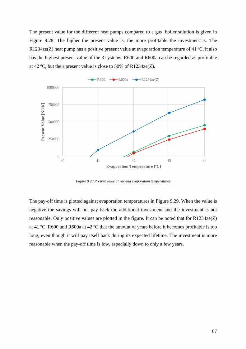
67

The present value for the different heat pumps compared to a gas boiler solution is given in

Figure 9.28. The higher the present value is, the more profitable the investment is. The

R1234ze(Z) heat pump has a positive present value at evaporation temperature of 41 ºC, it also

has the highest present value of the 3 systems. R600 and R600a can be regarded as profitable

at 42 ºC, but their present value is close to 50% of R1234ze(Z).

Figure 9.28 Present value at varying evaporation temperatures

The pay-off time is plotted against evaporation temperatures in Figure 9.29. When the value is

negative the savings will not pay back the additional investment and the investment is not

reasonable. Only positive values are plotted in the figure. It can be noted that for R1234ze(Z)

at 41 ºC, R600 and R600a at 42 ºC that the amount of years before it becomes profitable is too

long, even though it will pay itself back during its expected lifetime. The investment is more

reasonable when the pay-off time is low, especially down to only a few years.

0

250000

500000

750000

1000000

40 41 42 43 44

Pres

ent V

alue

[NO

K]


R600 R600a R1234ze(Z)

68

Figure 9.29 Pay-Off Time for different heat pump solution against a natural gas boiler


0

2

4

6

8

10

12

14

16

18

40 41 42 43 44

Pay-

Off

Tim

e [y

ears

]


R600 R600a R1234ze(Z)

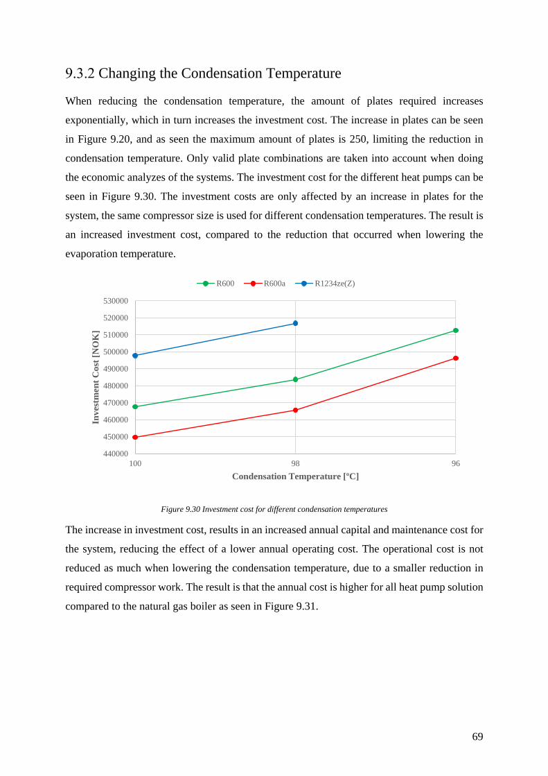
69

Changing the Condensation Temperature

When reducing the condensation temperature, the amount of plates required increases

exponentially, which in turn increases the investment cost. The increase in plates can be seen

in Figure 9.20, and as seen the maximum amount of plates is 250, limiting the reduction in

condensation temperature. Only valid plate combinations are taken into account when doing

the economic analyzes of the systems. The investment cost for the different heat pumps can be

seen in Figure 9.30. The investment costs are only affected by an increase in plates for the

system, the same compressor size is used for different condensation temperatures. The result is

an increased investment cost, compared to the reduction that occurred when lowering the

evaporation temperature.

Figure 9.30 Investment cost for different condensation temperatures

The increase in investment cost, results in an increased annual capital and maintenance cost for

the system, reducing the effect of a lower annual operating cost. The operational cost is not

reduced as much when lowering the condensation temperature, due to a smaller reduction in

required compressor work. The result is that the annual cost is higher for all heat pump solution

compared to the natural gas boiler as seen in Figure 9.31.

440000

450000

460000

470000

480000

490000

500000

510000

520000

530000

9698100

Inve

stm

ent C

ost [

NO

K]


R600 R600a R1234ze(Z)

70

Figure 9.31 Annual cost for different condensation temperatures

This is also shown in Figure 9.32 where the specific heating cost for the different heat pumps

is higher than the cost for the natural gas boiler.

Figure 9.32 Specific heating cost for the different systems

The result of the high annual cost can be seen when calculating the present value in Figure 9.33.

It is negative for all the system at the available condensation temperatures. Buying a heat pump

and trying to optimizing it by reducing the condensation temperature for the chosen scenario is

not a profitable investment, due to the high losses caused at the base evaporation temperature.

370000

380000

390000

400000

410000

420000

430000

9698100

Ann

ual C

ost [

NO

K/y

ear]


R600 R600a R1234ze(Z) Gas Boiler

0,4

0,41

0,42

0,43

0,44

0,45

0,46

0,47

0,48

9698100

Spec

ific

Hea

ting

Cos

t [N

OK

/kW

h]


R600 R600a R1234ze(Z) Natural Gas Boiler

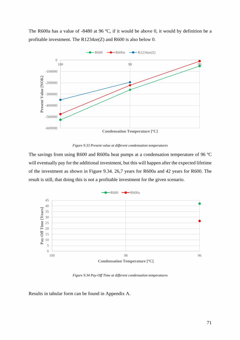
71

The R600a has a value of -8480 at 96 ºC, if it would be above 0, it would by definition be a

profitable investment. The R1234ze(Z) and R600 is also below 0.

Figure 9.33 Present value at different condensation temperatures

The savings from using R600 and R600a heat pumps at a condensation temperature of 96 ºC

will eventually pay for the additional investment, but this will happen after the expected lifetime

of the investment as shown in Figure 9.34. 26,7 years for R600a and 42 years for R600. The

result is still, that doing this is not a profitable investment for the given scenario.

Figure 9.34 Pay-Off Time at different condensation temperatures


-600000

-500000

-400000

-300000

-200000

-100000

09698100

Pres

ent V

alue

[NO

K]


R600 R600a R1234ze(Z)

05

1015202530354045

9698100

Pay-

Off

Tim

e [Y

ears

]


R600 R600a

72

Effect of Reduced Electricity Prices

The effect of a reduction in electricity price was investigated for R1234ze(Z). The change in

annual cost for the R1234ze(Z) heat pump at changing evaporation temperature can be seen in

Figure 9.35. As it is shown in the figure, the electricity price has a large impact of on the annual

cost of the system. With a reduction of 0,4 NOK/kWh the annual costs have a reduction of

approximately 125 000 NOK at 40 ºC and close to 100 000 NOK at 44 ºC.

Figure 9.35 Annual cost for R1234ze(Z) heat pump at changing electricity price

The effect on the present value can be seen in Figure 9.36. The present value has a large

increase, indicating a profitable investment, even at 40 ºC when the electricity price is 0,9

NOK/kWh. The investment gets a lot more profitable at lower electricity prices. The annual

costs have a large effect on the profitability of the system.

200000

225000

250000

275000

300000

325000

350000

375000

400000

425000

40 41 42 43 44

Ann

ual c

ost [

NO

K]

Evaporation temperature [ºC]

1,1 kr/kWh 0,9 kr/kWh 0,7 kr/kWh Gas 0,37 kr/kWh

73

Figure 9.36 Present value for R1234ze(Z) heat pump at changing electricity price

This is further shown when calculating the pay-off time in Figure 9.37. Only positive values

are plotted in the figure. The yearly saving is larger than the additional investment cost after

only 3 years at 41 ºC with an electricity price of 0,9 NOK/kWh, this is lower than the original

case even with an evaporation temperature of 44 ºC. For a price 0,7 NOK/kWh the system is

pay-off time is 2,4 years at 40 ºC and 1,4 years at 44 ºC. This shows that the profitability of the

investment is larger the closer the electricity prices is to the natural gas prices.

Figure 9.37 Pay-Off Time at varying electricity prices


0

500000

1000000

1500000

2000000

2500000

40 41 42 43 44

Pres

ent V

alue

[NO

K]

Evaporaiton Temperature [ºC]

1,1 kr/kWh 0,9 kr/kWh 0,7 kr/kWh

0

2

4

6

8

10

12

14

16

40 41 42 43 44

Pay-

Off

Tim

e [Y

ears

]


1,1 NOK/kWh 0,9 NOK/kWh 0,7 NOK/kWh

74

Effect of Reduced Natural Gas Prices

When reducing the natural gas price, while keeping the same electricity price the opposite effect

occurs. The difference in annual cost for the R1234ze(Z) heat pump gets smaller and smaller

compared to the natural gas boiler at increasing evaporation temperatures. This can be seen in

Figure 9.38. This reduces the savings for choosing a heat pump over a gas boiler, and can make

the investment in a heat pump unfeasible. The reduction in natural gas prices is not large, but it

has a large effect on the annual cost of the system.

Figure 9.38 Annual Cost for R1234ze(Z) heat pump and gas boiler at different natural gas prices

The bar chart in Figure 9.39 shows the present value for the R1234ze(Z) heat pump at different

evaporation temperatures with an electricity price of 1,1 NOK/kWh. As it shown in the chart,

the present value is reduced significantly. A low, but positive present value indicates that the

investment might be profitable, but not by much. At an evaporation temperature of 41 ºC the

heat pump is only profitable for a price of 0,37 NOK/kWh, while the lower natural gas prices

get more profitable at increasing evaporation temperatures. With a natural gas price of 0,32

NOK/kWh the investment is deemed profitable by definition at 44 ºC having a present value of

135660 NOK.

300000

325000

350000

375000

400000

425000

40 41 42 43 44

Ann

ual C

ost [

NO

K]


1,1 NOK/kWh Gas 0,37 NOK/kWh Gas 0,35 NOK/kWh

Gas 0,34 NOK/kWh Gas 0,33 NOK/kWh Gas 0,32 NOK/kWh

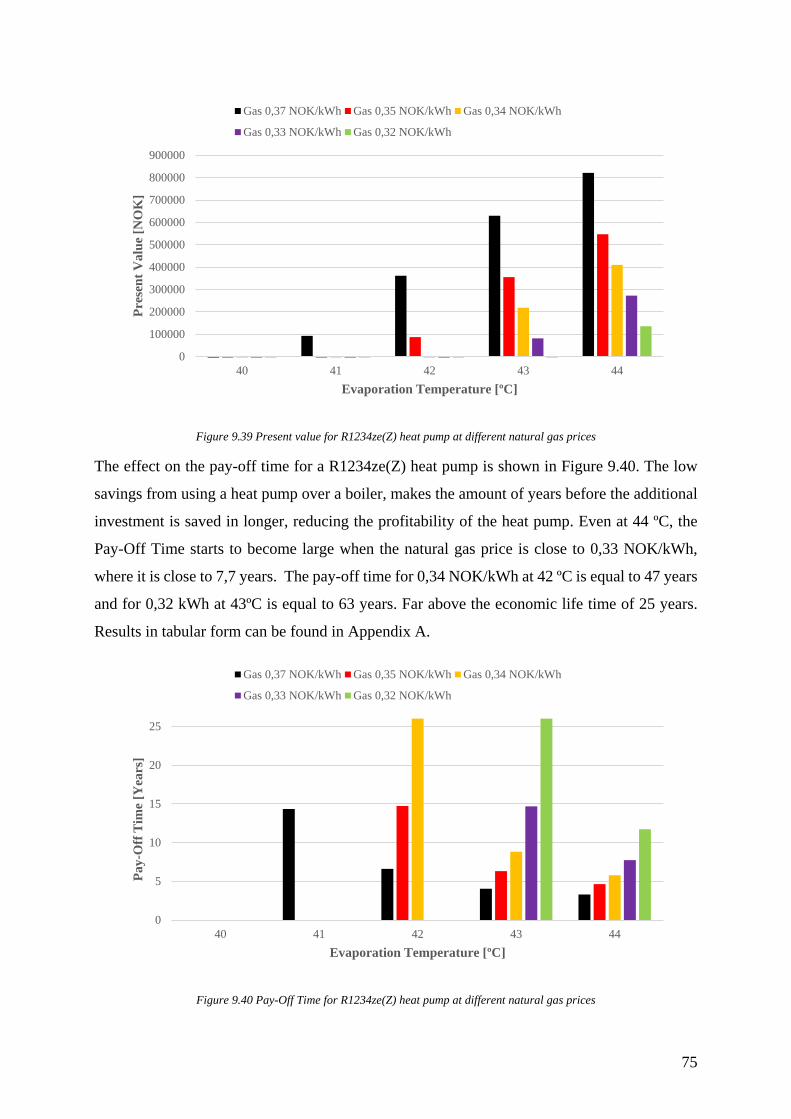
75

Figure 9.39 Present value for R1234ze(Z) heat pump at different natural gas prices

The effect on the pay-off time for a R1234ze(Z) heat pump is shown in Figure 9.40. The low

savings from using a heat pump over a boiler, makes the amount of years before the additional

investment is saved in longer, reducing the profitability of the heat pump. Even at 44 ºC, the

Pay-Off Time starts to become large when the natural gas price is close to 0,33 NOK/kWh,

where it is close to 7,7 years. The pay-off time for 0,34 NOK/kWh at 42 ºC is equal to 47 years

and for 0,32 kWh at 43ºC is equal to 63 years. Far above the economic life time of 25 years.


Figure 9.40 Pay-Off Time for R1234ze(Z) heat pump at different natural gas prices

0

100000

200000

300000

400000

500000

600000

700000

800000

900000

40 41 42 43 44

Pres

ent V

alue

[NO

K]



Gas 0,33 NOK/kWh Gas 0,32 NOK/kWh

0

5

10

15

20

25

40 41 42 43 44

Pay-

Off

Tim

e [Y

ears

]




76

Discussion

The results show that it is possible to save large amounts of energy by using a heat pump

solution over competing heating solutions. At the base operating conditions, the COP for the

cycle is close to 3 for R1234ze(Z) and 2,8 for R600 and R600a, which equals an energy saving

of close to 67% and 62% respectively. By further optimizing the operating conditions, the

energy saving will be close to 74% for R1234ze(Z), 71,5 % for R600 and 70,6 % for R600a.

The most efficient way to do this is by reducing the pressure drop over the evaporator, this is

done by increasing the evaporation temperature, increasing the size of the heat exchanger. The

best result was achieved with an evaporation temperature of 44 ºC which gives a pinch point

temperature of 1 K at the outlet of the evaporator, due to the 5 K superheat.

The reduction in pressure drop results in a reduction in the required compressor work of close

to 30% from 40 ºC to 44 ºC. This is because of a reduced temperature lift and an increase is

isentropic efficiency, due to a reduction in pressure ratio in ( 7.32 ). An efficient compressor

reduces discharge temperature, reducing the required area for desuperheating in the condenser,

resulting in a reduction in the condenser size. Another positive effect of a reduction in pressure

ratio is an increase in volumetric efficiency in ( 7.33 ) and an increase in vapor density, reducing

the required compressor volume, reducing the size of the compressor. The compressor work

and size has a large contributing factor on the annual cost of the system. Optimizing the

compressor work is essential, when wanting an efficient system.

By increasing the evaporation temperature, the increase in number of required channels is

moderate compared to decreasing the condensation temperature, where the increase of required

channels is exponential. The end result is that optimizing the cycle by just decreasing the

condensation temperature will end up being restricted by maximum number of plates allowed

in the exchanger. At an evaporation temperature of 40 ºC, R1234ze(Z) gets restricted before 96

ºC while R600 and R600a can operate at 96 ºC. This is due to a large required area for

desuperheating, due to the high pressure losses at 40 ºC. However, the performance increase

for reducing the condensation temperature is larger for R600 and R600a, due to having a lower

pressure drop in the evaporator compared to R1234ze(Z) and due to them having a smaller

superheat than R1234ze(Z). By increasing the evaporation temperature and reducing the

pressure loss in evaporator is possible to reach a lower condensation temperature, but this is not

assessed in the thesis.

77

When evaluating the results, it is important to take into account that basis of the model. The

correlations used for heat transfer and friction factor calculations in both the evaporator and

condenser is based on experimental data that is measured in the temperature range of 10-20 ºC

for the evaporator and 20-40 ºC for the condenser. The measurements are done for several

different refrigerants, including HFCs, HFOs(R1234ze(E) and yf) and natural refrigerants

(R600a, R290, etc.), but not for R600 and R1234ze(Z). Longo et al. (2014) suggested that

R1234ze(Z) should have higher heat transfer coefficients than the other refrigerants, including

R600a and a frictional pressure drop equal to R600a. The results from the model used in this

thesis is that the heat transfer coefficients are smaller but the pressure drop is of similar

magnitude.

Another important factor that would affect the results is the geometry and the flow conditions

inside the heat exchanger. Similar hydraulic diameter and chevron angle is however chosen to

minimize this effect. As seen in the results, the chevron angle has a large effect on the pressure

drop and heat transfer in the evaporator. In the condenser correlations this effect is not taken

into consideration other than a change in enlargement factor and increased heat transfer from

the water.

The heat exchangers are modelled as parallel-flow heat exchangers, resulting in a large

temperature difference at the inlet of the condenser. Using a counter-flow configuration could

increase the heat exchanger efficiency.

With the chosen step size the control volume length is 1 cm and for instance if the wanted

subcooling is not reach the iteration will run 1 more step causing a lower exit temperature than

wanted, this can be resolved by reducing the step size, increasing the accuracy of the

calculation. However, the effect on the results are small and the chosen step size gives a

sufficient accuracy overall.

In regards to the economic evaluations, it can be seen that the annual costs are heavily affected

by the annual operating costs. None of the cycle improvements added more to the investment

costs than it saved in operating costs. This could be different if the COP was a lot higher, since

the reduction in energy saving per COP will be smaller at increasing COP. When the difference

in electricity and natural gas prices is as large as it is, it is important to optimize the heat pump

solution to have get a profitable investment. The bigger the difference in annual costs between

the two system, the more profitable an investment will be.

78

The most cost efficient way to optimize the heat pump was in this case to increase the

evaporation temperature, increasing the heat transfer area, thus reducing the pressure loss. This

resulted in a smaller temperature lift, an increased compressor efficiency and a smaller required

compressor volume. The importance of reducing the losses can also be seen in the results when

only reducing the condensation temperature, where the annual cost was not reduced enough to

make the system profitable. It can be noted that the R600 and R600a cycles both had an

additional pressure loss that was constant due to the need of a suction gas heat exchanger, which

resulted in reduced efficiency and slightly added investment cost. A larger suction gas heat

exchanger with reduced pressure loss could increase the cycles efficiency and make them more

profitable.

From the sensitivity analysis it can be seen that for low electricity prices has a large effect on

the annual costs, and countries with cheap electricity, like Norway, have a higher chance of

making heat pumps a profitable investment than countries with high electricity prices. A lower

electricity price also opens up for a larger investment, making it possible to increase the

efficiency even further. The gas prices could not decrease much before the R1234ze(Z) heat

pump would be unprofitable. With increased awareness on global warming, it is not

unreasonable to assume an increase in the price for fossil fuels or increased taxation on CO2,

which will further favor a heat pump solution using environmental friendly refrigerants.

R600a has the lowest compressor volume of the 3 refrigerants, and in the economic evaluations

the compressor price is therefore lower for it than for R600 and R1234ze(Z). However, for the

chosen compressor series the compressor had to run at a 1000 RPM with R600a instead of 1500

RPM as it does with R600 which the price is based on. Resulting in larger and more expensive

compressors for R600a than for R600, further reducing the advantages of R600a compared to

R600 and R1234ze(Z). The suppliers that were contacted had no compressors that was available

for R1234ze(Z) as of now, so the compressor cost was assumed to be similar to a R600

compressor.

The results of this thesis shows that both R600 and R1234ze(Z) has a better operating efficiency

than R600a, and in reality the investment costs might be higher for R600a than they are for

R600 as discussed above. Resulting in lower annual costs for R600 and R1234ze(Z). Ommen

et al. (2015) results indicate that R600a is the most suitable of refrigerants they investigate for

high sink temperatures. This would imply that both R600 and R1234ze(Z) are an even better

choice for high sink temperatures.

79

Another thing to be noted is that the investment costs calculated only contains the components

costs and not additional costs that could increase the total cost of the systems; installation costs,

safety measures due to flammability, refrigerant cost, valves, control system etc. It is also

possible to invest in in two smaller systems that covers the heat duty together, for increased

flexibility and safety at the cost of increased annual costs. This would decrease the profitability

against the natural gas boiler, but with a properly optimized cycle it should be possible. Another

alternative is two separate systems that can cover the entire load for increased operational

reliability.

All of the selected refrigerants are regarded as flammable, however R1234ze(Z) is considered

to be mildly flammable. This might be the deciding factor when it comes to getting acceptance

by the consumer. Required safety measures are however, not assessed in this thesis, and

therefore suggested for further investigation.

80

Conclusion

Heat pumps have the potential to reduce the energy consumption in industrial heating processes

and at the same time being a profitable investment, even in markets where the electricity prices

are a lot higher than fossil alternatives. However, the importance of optimizing the cycle is

increasingly important when the electricity prices are high. A heat pump might cost less to

operate yearly than a natural gas boiler, but if the savings are minimal the additional investment

might result in an unprofitable investment. It is therefore important to do economic evaluations

when considering in investing in a heat pump solution.

A heat pump model using environmental friendly refrigerants were developed for a given case

and used to investigate different operating conditions, and their effect on the systems

profitability when compared to a natural gas boiler.

The main results from the simulation are:

• R1234ze(Z) achieves the highest COP of 3,8 with an evaporation temperature of 44 ºC,

this results in an annual cost of 325 000 NOK/year and a Pay-Off Time of 3,3 years

compared to a gas boiler.

• R1234ze(Z) achieves the second highest COP of 3,6 at 43 ºC this results in an annual

cost of 339 000 NOK/year and a Pay-Off Time of 4 years compared to a gas boiler.

• R600 achieves the third highest COP of 3,5 with an evaporation temperature of 44 ºC

this results in an annual cost of 352 000 NOK/year and a Pay-Off Time of 5,4 years

compared to a gas boiler.

• R600a achieves the lowest performance of the 3 refrigerants, maximum COP of 3,4 with

an evaporation temperature of 44 ºC, this results in an annual cost of 356 000 NOK/year

and a Pay-Off Time of 5,5 years compared to a gas boiler.

• Using R1234ze(Z) or R600 would be a better choice than R600a for high temperature

heat pumps.

• The operational cost is the biggest contribution to the annual cost. All tested cycle

improvements saved more money from operational cost than it added to the capital

costs.

• When there is a big difference in natural gas and electricity prices a poorly optimized

heat pump is not a profitable investment compared to a natural gas boiler. A heat pump

that is better optimized will be able to handle an even larger price difference and still be

profitable.

81

• The profitability of a heat pump investment will be a lot higher at reduced electricity

prices, allowing for larger investments.

• Pressure drop in the evaporator has a significant impact of the performance and

profitability of the system.

• Keeping a high pressure drop over the evaporator and only reducing the condensation

resulted in a system that was not profitable.

Suggestions for Further Work Based on the work carried out, the following are suggested to be investigated further:

• Investigate the effect of using flooded evaporators in regards to increased evaporation

temperatures and the effect on the annual cost.

• Investigate the effect of using counter-flow heat exchangers over parallel-flow heat

exchangers.

• Optimize the size of the suction gas heat exchanger to find the most efficient size in

regards to pressure drop and investment cost.

• Optimize the heat pump cycle in regards to finding the optimal evaporation and

condensation temperature.

• Investigate required safety measures for the different refrigerants and their cost.

• Do simulations with other refrigerants (i.e. HFO1336mzz(Z), ammonia) when property

data and new correlations are available.

82

Bibliography

AMALFI, R. L., VAKILI-FARAHANI, F. & THOME, J. R. 2016a. Flow boiling and frictional pressure gradients in plate heat exchangers. Part 1: Review and experimental database. International Journal of Refrigeration, 61, 166-184.

AMALFI, R. L., VAKILI-FARAHANI, F. & THOME, J. R. 2016b. Flow boiling and frictional pressure gradients in plate heat exchangers. Part 2: Comparison of literature methods to database and new prediction methods. International Journal of Refrigeration, 61, 185-203.

ASSAF, K., ZOUGHAIB, A., SAPORA, E., PEUREUX, J.-L. & CLODIC, D. 2010. Experimental Simulation of a Heat Recovery Heat Pump System in Food Industries. International Refrigeration and Air Conditioning Conference. Purdue University: Purdue e-Pubs.

AUSTIN, B. T. & SUMATHY, K. 2011. Transcritical carbon dioxide heat pump systems: A review. Renewable and Sustainable Energy Reviews, 15, 4013-4029.

BERGLAND, M., EIKEVIK, T. M. & TOLSTOREBROV, I. 2015. OPTIMIZING THE COMPRESSION/ABSORPTION HEAT PUMP SYSTEM AT HIGH TEMPERATURES. ICR 2015. Yokohama, Japan.

BERTINAT, M. P. 1986. Fluids for high temperature heat pumps. International Journal of Refrigeration, 9, 43-50.

BOBELIN, D., BOURIG, A. & PEUREUX, J. L. 2012. Experimental results of a new developed very high temperature industrial heat pump (140°C) equipped with scroll compressors and working with a new blend refrigerant. International Refrigeration and Air Conditioning Conference. Purdue University, USA: Purdue e-Pubs.

BROBERG VIKLUND, S. & JOHANSSON, M. T. 2014. Technologies for utilization of industrial excess heat: Potentials for energy recovery and CO2 emission reduction. Energy Conversion and Management, 77, 369-379.

BROWN, J. S., ZILIO, C. & CAVALLINI, A. 2009. The fluorinated olefin R-1234ze(Z) as a high-temperature heat pumping refrigerant. International Journal of Refrigeration, 32, 1412-1422.

BRÜCKNER, S., LIU, S., MIRÓ, L., RADSPIELER, M., CABEZA, L. F. & LÄVEMANN, E. 2015. Industrial waste heat recovery technologies: An economic analysis of heat transformation technologies. Applied Energy, 151, 157-167.

BÄCKSTRÖM, M. 1946. Kylteknikern del 1, Stockholm, Svenska Kyltekniska Föreningen. CALM, J. M. 2008. The next generation of refrigerants – Historical review, considerations,

and outlook. International Journal of Refrigeration, 31, 1123-1133. CAVALLINI, A., COL, D. D., DORETTI, L., MATKOVIC, M., ROSSETTO, L., ZILIO, C.

& CENSI, G. 2006. Condensation in Horizontal Smooth Tubes: A New Heat Transfer Model for Heat Exchanger Design. Heat Transfer Engineering, 27, 31-38.

CHAMOUN, M., RULLIERE, R., HABERSCHILL, P. & PEUREUX, J.-L. 2012. Experimental Investigation of a New High Temperature Heat Pump Using Water as Refrigerant for Industrial Heat Recovery. International Refrigeration and Air Conditioning Conference. Purdue University, USA: Purdue e-Pubs.

CHAMOUN, M., RULLIERE, R., HABERSCHILL, P. & PEUREUX, J.-L. 2014. Experimental and numerical investigations of a new high temperature heat pump for

83

industrial heat recovery using water as refrigerant. International Journal of Refrigeration, 44, 177-188.

CHRISTENSEN, S. W., ELMEGAARD, B., MARKUSSEN, W. B., ROTHUIZEN, E. & MADSEN, C. 2015. MODELLING OF AMMONIA HEAT PUMP DESUPERHEATERS. ICR 2015. Yokohama, Japan.

CHUA, K. J., CHOU, S. K. & YANG, W. M. 2010. Advances in heat pump systems: A review. Applied Energy, 87, 3611-3624.

DANFOSS 2016. Coolselector®2. DEVOTTA, S. & RAO PENDYALA, V. 1994. Thermodynamic screening of some HFCs and

HFEs for high-temperature heat pumps as alternatives to CFC114. International Journal of Refrigeration, 17, 338-342.

EIKEVIK, T. M. 13.05 2016. RE: Personal communication. EIKEVIK, T. M., TOLSTOREBROV, I., BREDESEN, A. M., REKSTAD, H., PETTERSEN,

J., AFLEKT, K. & ELGSÆTHER, M. 2016. TEP 4255 - Heat pumping processes and systems, NTNU, NTNU EPT.

EKROTH, I. & GRANRYD, E. 2009. The vapor compression cycle. Refrigerating Engineering. Royal Institute of Technology, KTH.

ELDEEB, R., AUTE, V. & RADERMACHER, R. 2016. A survey of correlations for heat transfer and pressure drop for evaporation and condensation in plate heat exchangers. International Journal of Refrigeration, 65, 12-26.

EUROSTAT. 2016. Energy Price Statistics [Online]. Luxembourg: Eurostat Available: http://ec.europa.eu/eurostat/statistics-explained/index.php/Energy_price_statistics [Accessed 24.05 2016].

FUKUDA, S., KONDOU, C., TAKATA, N. & KOYAMA, S. 2014. Low GWP refrigerants R1234ze(E) and R1234ze(Z) for high temperature heat pumps. International Journal of Refrigeration, 40, 161-173.

GARCÍA-CASCALES, J. R., VERA-GARCÍA, F., CORBERÁN-SALVADOR, J. M. & GONZÁLVEZ-MACIÁ, J. 2007. Assessment of boiling and condensation heat transfer correlations in the modelling of plate heat exchangers. International Journal of Refrigeration, 30, 1029-1041.

GRANRYD, E. 2001. Hydrocarbons as refrigerants — an overview. International Journal of Refrigeration, 24, 15-24.

HAUKÅS, H. T. 2015. Norsk Kulde- og Varmepumpenorm, Norsk Kjøleteknisk Forening. IEA-HPC 2014a. Application of Industrial Heat Pumps, Part 1. IEA HPP ANNEX 35.

International Energy Agency Heat Pump Centre. IEA-HPC 2014b. Application of Industrial Heat Pumps, Part 2. IEA HPP ANNEX 35.

International Energy Agency Heat Pump Centre. JANA, A. K. & MAITI, D. 2013. Assessment of the implementation of vapor recompression

technique in batch distillation. Separation and Purification Technology, 107, 1-10. JENSEN, J. K., MARKUSSEN, W. B., REINHOLDT, L. & ELMEGAARD, B. 2015a. On

the development of high temperature ammonia-water hybrid absorption-compression heat pumps. International Journal of Refrigeration.

JENSEN, J. K., OMMEN, T., MARKUSSEN, W. B., REINHOLDT, L. & ELMEGAARD, B. 2015b. Technical and economic working domains of industrial heat pumps: Part 2 –

http://ec.europa.eu/eurostat/statistics-explained/index.php/Energy_price_statistics

84

Ammonia-water hybrid absorption-compression heat pumps. International Journal of Refrigeration, 55, 183-200.

JOHNSON CONTROLS NORWAY. 26.05 2016. RE: Email communication: Forespørsel om priser til masteroppgave ved NTNU.

KAZEMI, A., HOSSEINI, M., MEHRABANI-ZEINABAD, A. & FAIZI, V. 2016. Evaluation of different vapor recompression distillation configurations based on energy requirements and associated costs. Applied Thermal Engineering, 94, 305-313.

KIM, J., PARK, S.-R., BAIK, Y.-J., CHANG, K.-C., RA, H.-S., KIM, M. & KIM, Y. 2013. Experimental study of operating characteristics of compression/absorption high-temperature hybrid heat pump using waste heat. Renewable Energy, 54, 13-19.

KIM, M.-H., PETTERSEN, J. & BULLARD, C. W. 2004. Fundamental process and system design issues in CO2 vapor compression systems. Progress in Energy and Combustion Science, 30, 119-174.

KLEIN, S. 2015. Engineering Equation Solver Professional 9.935-3D. Madison, WI: F-Chart Software.

KONDOU, C. & KOYAMA, S. 2015. Thermodynamic assessment of high-temperature heat pumps using Low-GWP HFO refrigerants for heat recovery. International Journal of Refrigeration, 53, 126-141.

KONTOMARIS, K. 2012. A ZERO-ODP, LOW GWP WORKING FLUID FOR HIGH TEMPERATURE HEATING AND POWER GENERATION FROM LOW TEMPERATURE HEAT: DR-2. THE INTERNATIONAL SYMPOSIUM on NEW REFRIGERANTS and ENVIRONMENTAL TECHNOLOGY 2012. Kobe, Japan: The Japan Refrigeration and Air Conditioning Industry Association.

KONTOMARIS, K. 2014. HFO-1336mzz-Z: High Temperature Chemical Stability and Use as A Working Fluid in Organic Rankine Cycles. International Refrigeration and Air Conditioning Conference. Purdue University: Purdue e-Pubs.

KONTOMARIS, K. 2016. Low GWP Refrigerants for Efficient Cooling, Heating and Power Generation. IEA Heat Pump Centre Newsletter. IEA Heat Pump centre.

LEMMON, E., HUBER, M. & MCLINDEN, M. Refprop 9.0, NIST standard reference database 23, Version 9.0 2010. USA.

LONGO, G. A. 2010. Heat transfer and pressure drop during hydrocarbon refrigerant condensation inside a brazed plate heat exchanger. International Journal of Refrigeration, 33, 944-953.

LONGO, G. A., MANCIN, S., RIGHETTI, G. & ZILIO, C. 2015a. A new model for refrigerant boiling inside Brazed Plate Heat Exchangers (BPHEs). International Journal of Heat and Mass Transfer, 91, 144-149.

LONGO, G. A., RIGHETTI, G. & ZILIO, C. 2015b. A new computational procedure for refrigerant condensation inside herringbone-type Brazed Plate Heat Exchangers. International Journal of Heat and Mass Transfer, 82, 530-536.

LONGO, G. A., ZILIO, C., RIGHETTI, G. & BROWN, J. S. 2014. Experimental assessment of the low GWP refrigerant HFO-1234ze(Z) for high temperature heat pumps. Experimental Thermal and Fluid Science, 57, 293-300.

MA, Y., LIU, Z. & TIAN, H. 2013. A review of transcritical carbon dioxide heat pump and refrigeration cycles. Energy, 55, 156-172.

85

MADSBOELL, H., WEEL, M. & KOLSTRUP, A. 2015. DEVELOPMENT OF A WATER VAPOR COMPRESSOR FOR HIGH TEMPERATURE HEAT PUMP APPLICATIONS. ICR 2015. Yokohama, Japan.

MARTIN, H. 1996. A theoretical approach to predict the performance of chevron-type plate heat exchangers. Chemical Engineering and Processing: Process Intensification, 35, 301-310.

MCLINDEN, M. O., KAZAKOV, A. F., STEVEN BROWN, J. & DOMANSKI, P. A. 2014. A thermodynamic analysis of refrigerants: Possibilities and tradeoffs for Low-GWP refrigerants. International Journal of Refrigeration, 38, 80-92.

NEKSÅ, P., REKSTAD, H., ZAKERI, G. R. & SCHIEFLOE, P. A. 1998. CO2-heat pump water heater: characteristics, system design and experimental results. International Journal of Refrigeration, 21, 172-179.

NELLIS, G. & KLEIN, S. 2009. Heat transfer, Cambridge, Cambridge University Press. NORDTVEDT, S. R. 2005. Experimental and theoretical study of a compression/absorption

heat pump with ammonia/water as working fluid. Norwegian University of Science and Technology.

NORDTVEDT, S. R., HORNTVEDT, B. R., EIKEFJORD, J. & JOHANSEN, J. 2013. Hybrid heat pump for waste heat recovery in norwegian food industry. Thermally driven heat pumps for heating and cooling. Berlin: Universitätsverlag der TU Berlin.

OLULEYE, G., JOBSON, M., SMITH, R. & PERRY, S. J. 2016. Evaluating the potential of process sites for waste heat recovery. Applied Energy, 161, 627-646.

OMMEN, T., JENSEN, J. K., MARKUSSEN, W. B., REINHOLDT, L. & ELMEGAARD, B. 2015. Technical and economic working domains of industrial heat pumps: Part 1 – Single stage vapour compression heat pumps. International Journal of Refrigeration, 55, 168-182.

PACHAI, A. C. & HARRAGHY, P. 2013. Practical experience of applying ammonia and hydrocarbon refrigeration systems for standard refrigeration and air conditioning applications – part two. Ecolibrium, 46-51.

PALM, B. 2014. Köldmedier med låg GWP (HFO). KTH. PAN, L., WANG, H., CHEN, Q. & CHEN, C. 2011. Theoretical and experimental study on

several refrigerants of moderately high temperature heat pump. Applied Thermal Engineering, 31, 1886-1893.

PEARSON, A. 2012. High temperature heat pumps with natural refrigerants. IEA HEAT PUMP CENTRE IEA NEWSLETTER VOL. 30 1/2012. IEA.

QU, M. & ABDELAZIZ, O. 2015. IMPROVING WATER AND ENERGY EFFICIENCY OF POWER PLANT THROUGH ABSORPTION HEAT PUMP. ICR 2015. Yokohama, Japan.

SARKAR, J., BHATTACHARYYA, S. & GOPAL, M. R. 2004. Optimization of a transcritical CO2 heat pump cycle for simultaneous cooling and heating applications. International Journal of Refrigeration, 27, 830-838.

SARKAR, J., BHATTACHARYYA, S. & RAM GOPAL, M. 2007. Natural refrigerant-based subcritical and transcritical cycles for high temperature heating. International Journal of Refrigeration, 30, 3-10.

86

SHAH, R. K. & SEKULIĆ, D. P. 2007. Heat Exchanger Design Procedures. Fundamentals of Heat Exchanger Design. John Wiley & Sons, Inc.

SOROKA, B. 2015. Application Note – Industrial Heat Pumps. Leonardo Energy. STENE, J. 1993. VARMEPUMPER - Industrielle anvendelser, NTH-SINTEF Kuldeteknikk. STENE, J. 1997. Varmepumper Grunnleggende varmepumpeteknikk, SINTEF

Energiforskning AS. STENE, J. 2016. Investment Analysis for Heat Pump Systems. TEP4260 Presentation.

NTNU. SWEP 2016. SSP G7. 7.0.3.54 ed. UDAY BHASKAR BABU, G. & JANA, A. K. 2014. Impact of vapor recompression in batch

distillation on energy consumption, cost and CO2 emission: Open-loop versus closed-loop operation. Applied Thermal Engineering, 62, 365-374.

WANG, L., SUNDÉN, B. & MANGLIK, R. M. 2007. Plate heat exchangers : design, applications and performance, Southampton, WITPress.

88

Appendix A Supplements P-h diagrams and temperature distributions in the heat exchangers for the different refrigerants for evaporation temperatures of 40 ºC and 44 ºC and condensation temperature of 100 ºC can be seen below. Results from the simulations is also found in tables below.

Figure A.1 P-h diagram for R600 at 40/100 ºC

Figure A.2 P-h diagram for R600 at 44/100 ºC

4,0x105 5,0x105 6,0x105 7,0x105 8,0x105105

106

5x106

h [J/kg]

P [P

a]

316,2 K

368,4 K

R600

4,0x105 5,0x105 6,0x105 7,0x105 8,0x105105

106

5x106

h [J/kg]

P [P

a]

316,2 K

368,4 K

R600

89

Figure A.3 P-h diagram for R600a at 40/100 ºC

Figure A.4 P-h diagram for R600a at 44/100 ºC

4,4x105 5,0x105 5,5x105 6,1x105 6,6x105 7,2x1053x105

5x105

106

2x106

5x106

h [J/kg]

P [P

a]

316,2 K

368,4 K

R600a

4,4x105 5,0x105 5,5x105 6,1x105 6,6x105 7,2x1053x105

5x105

106

2x106

5x106

h [J/kg]

P [P

a]

316,2 K

368,4 K

R600a

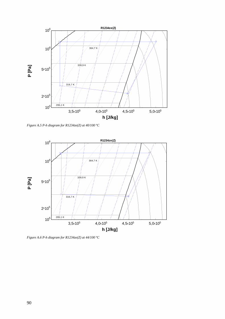
90

Figure A.5 P-h diagram for R1234ze(Z) at 40/100 ºC

Figure A.6 P-h diagram for R1234ze(Z) at 44/100 ºC

3,5x105 4,0x105 4,5x105 5,0x105105

2x105

5x105

106

106

h [J/kg]

P [P

a]

295,1 K

316,7 K

339,9 K

364,7 K

R1234ze(Z)

3,5x105 4,0x105 4,5x105 5,0x105105

2x105

5x105

106

106

h [J/kg]

P [P

a]

295,1 K

316,7 K

339,9 K

364,7 K

R1234ze(Z)

91

Figure A.7 Temperature distribution in condenser for R600 at 40 ºC

Figure A.8 Temperature distribution in evaporator for R600 at 40 ºC

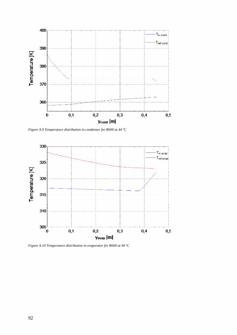
92

Figure A.9 Temperature distribution in condenser for R600 at 44 ºC

Figure A.10 Temperature distribution in evaporator for R600 at 44 ºC

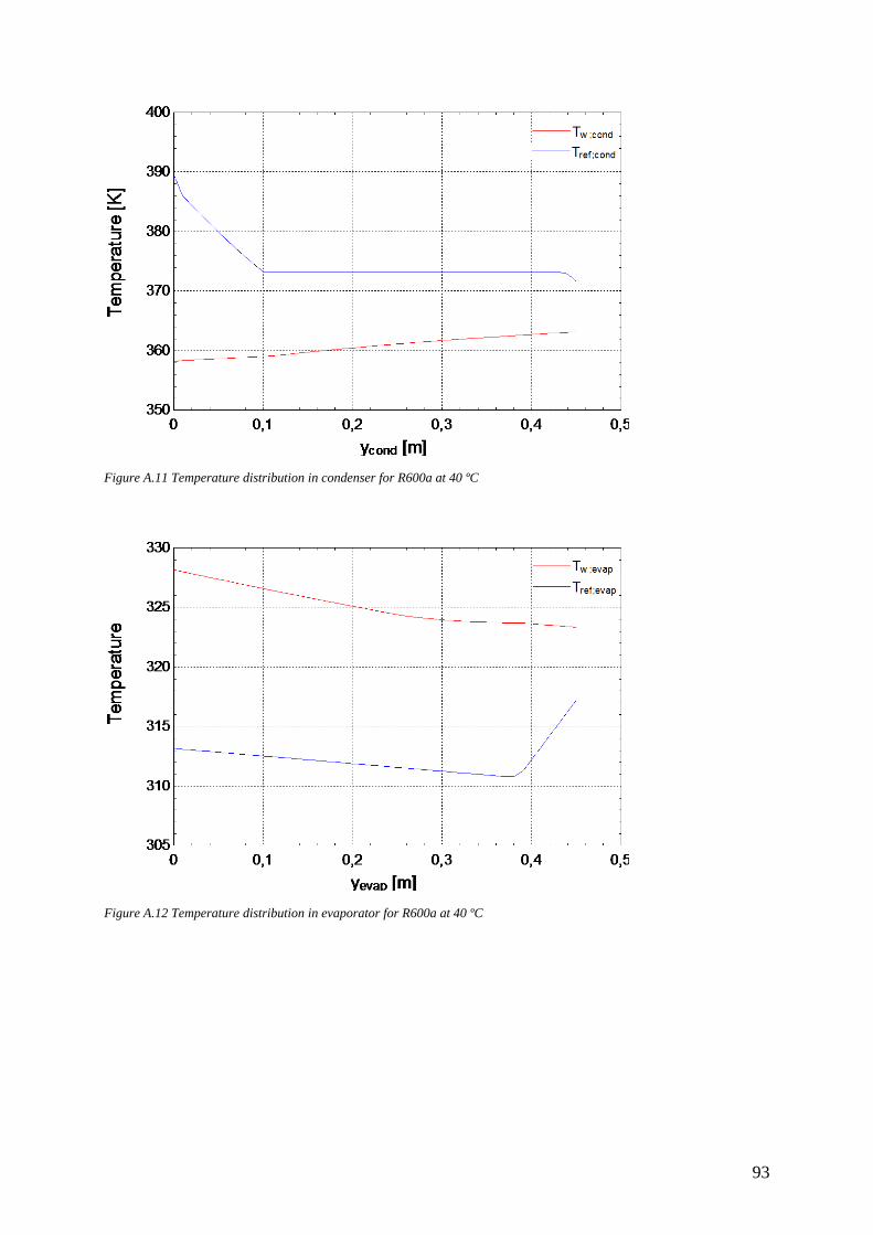
93

Figure A.11 Temperature distribution in condenser for R600a at 40 ºC

Figure A.12 Temperature distribution in evaporator for R600a at 40 ºC

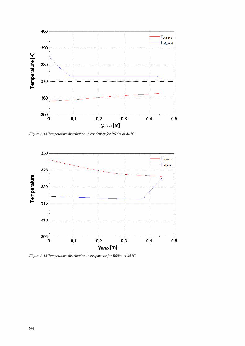
94

Figure A.13 Temperature distribution in condenser for R600a at 44 ºC

Figure A.14 Temperature distribution in evaporator for R600a at 44 ºC

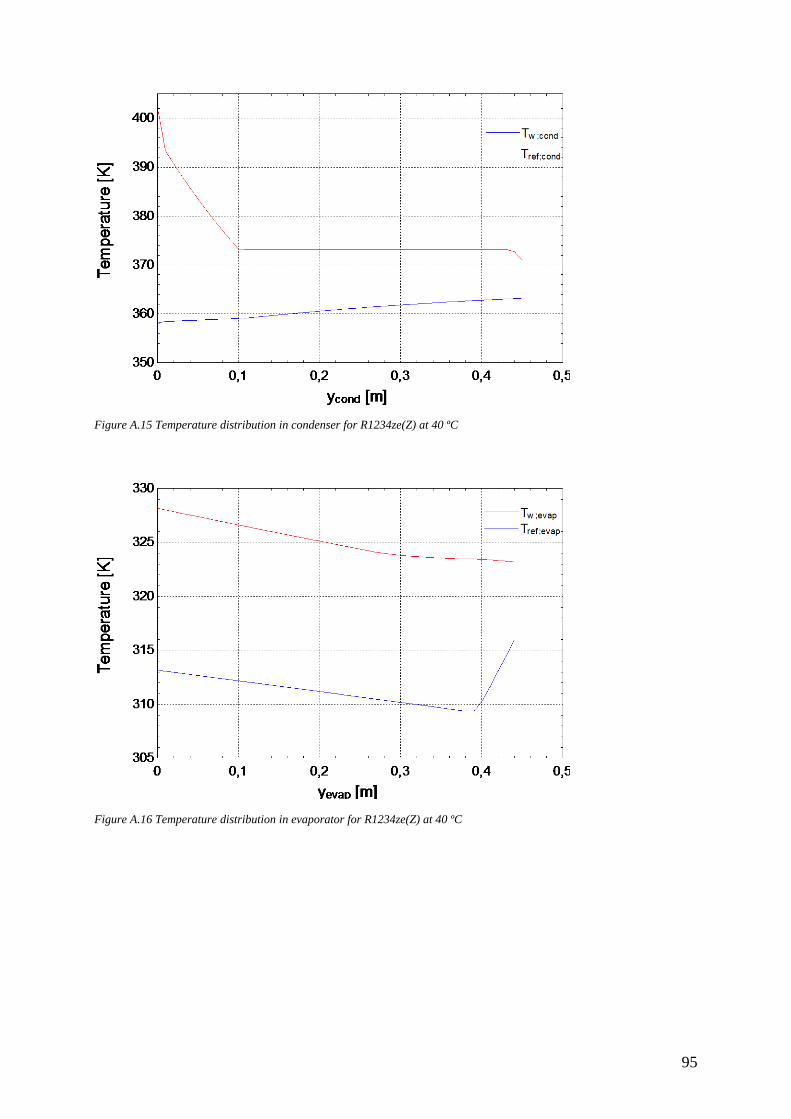
95

Figure A.15 Temperature distribution in condenser for R1234ze(Z) at 40 ºC

Figure A.16 Temperature distribution in evaporator for R1234ze(Z) at 40 ºC

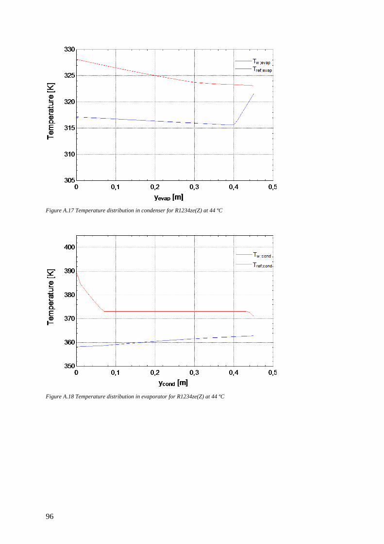
96

Figure A.17 Temperature distribution in condenser for R1234ze(Z) at 44 ºC

Figure A.18 Temperature distribution in evaporator for R1234ze(Z) at 44 ºC

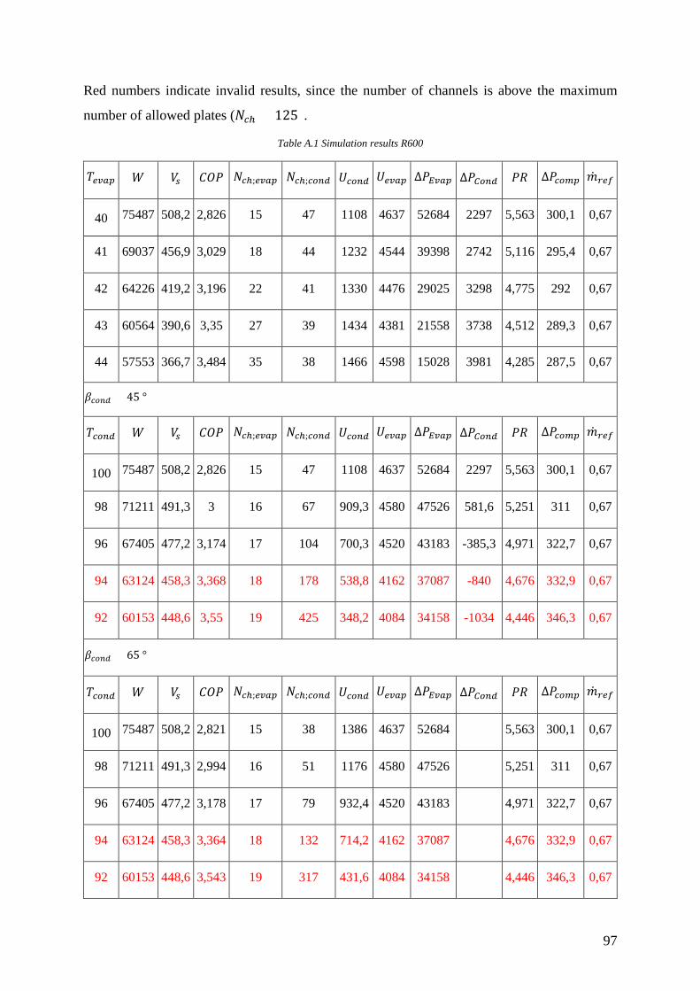
97

Red numbers indicate invalid results, since the number of channels is above the maximum

number of allowed plates (𝑁𝑁𝑐𝑐ℎ > 125).

Table A.1 Simulation results R600

𝑇𝑇𝑟𝑟𝑣𝑣𝑚𝑚𝑡𝑡 𝑊𝑊 𝑉𝑉𝑠𝑠 𝐶𝐶𝑃𝑃𝑃𝑃 𝑁𝑁𝑐𝑐ℎ;𝑟𝑟𝑣𝑣𝑚𝑚𝑡𝑡 𝑁𝑁𝑐𝑐ℎ;𝑐𝑐𝑙𝑙𝑐𝑐𝑐𝑐 𝑈𝑈𝑐𝑐𝑙𝑙𝑐𝑐𝑐𝑐 𝑈𝑈𝑟𝑟𝑣𝑣𝑚𝑚𝑡𝑡 Δ𝑃𝑃𝐸𝐸𝑣𝑣𝑚𝑚𝑡𝑡 Δ𝑃𝑃𝐶𝐶𝑙𝑙𝑐𝑐𝑐𝑐 𝑃𝑃𝑅𝑅 Δ𝑃𝑃𝑐𝑐𝑙𝑙𝑚𝑚𝑡𝑡 �̇�𝑚𝑟𝑟𝑟𝑟𝑟𝑟

40 75487 508,2 2,826 15 47 1108 4637 52684 2297 5,563 300,1 0,67

41 69037 456,9 3,029 18 44 1232 4544 39398 2742 5,116 295,4 0,67

42 64226 419,2 3,196 22 41 1330 4476 29025 3298 4,775 292 0,67

43 60564 390,6 3,35 27 39 1434 4381 21558 3738 4,512 289,3 0,67

44 57553 366,7 3,484 35 38 1466 4598 15028 3981 4,285 287,5 0,67

𝛽𝛽𝑐𝑐𝑙𝑙𝑐𝑐𝑐𝑐 = 45 °

𝑇𝑇𝑐𝑐𝑙𝑙𝑐𝑐𝑐𝑐 𝑊𝑊 𝑉𝑉𝑠𝑠 𝐶𝐶𝑃𝑃𝑃𝑃 𝑁𝑁𝑐𝑐ℎ;𝑟𝑟𝑣𝑣𝑚𝑚𝑡𝑡 𝑁𝑁𝑐𝑐ℎ;𝑐𝑐𝑙𝑙𝑐𝑐𝑐𝑐 𝑈𝑈𝑐𝑐𝑙𝑙𝑐𝑐𝑐𝑐 𝑈𝑈𝑟𝑟𝑣𝑣𝑚𝑚𝑡𝑡 Δ𝑃𝑃𝐸𝐸𝑣𝑣𝑚𝑚𝑡𝑡 Δ𝑃𝑃𝐶𝐶𝑙𝑙𝑐𝑐𝑐𝑐 𝑃𝑃𝑅𝑅 Δ𝑃𝑃𝑐𝑐𝑙𝑙𝑚𝑚𝑡𝑡 �̇�𝑚𝑟𝑟𝑟𝑟𝑟𝑟

100 75487 508,2 2,826 15 47 1108 4637 52684 2297 5,563 300,1 0,67

98 71211 491,3 3 16 67 909,3 4580 47526 581,6 5,251 311 0,67

96 67405 477,2 3,174 17 104 700,3 4520 43183 -385,3 4,971 322,7 0,67

94 63124 458,3 3,368 18 178 538,8 4162 37087 -840 4,676 332,9 0,67

92 60153 448,6 3,55 19 425 348,2 4084 34158 -1034 4,446 346,3 0,67



100 75487 508,2 2,821 15 38 1386 4637 52684 5,563 300,1 0,67

98 71211 491,3 2,994 16 51 1176 4580 47526 5,251 311 0,67

96 67405 477,2 3,178 17 79 932,4 4520 43183 4,971 322,7 0,67

94 63124 458,3 3,364 18 132 714,2 4162 37087 4,676 332,9 0,67

92 60153 448,6 3,543 19 317 431,6 4084 34158 4,446 346,3 0,67

98

Table A.2 Simulation results R600a


40 73760 376,8 2,835 14 45 1218 4724 63781 4358 4,789 298,9 0,8

41 69122 348,7 2,966 16 42 1308 4629 51757 5128 4,505 295,2 0,8

42 64878 322,4 3,123 20 40 1386 4510 37039 5741 4,226 292,8 0,8

43 61733 302,8 3,27 25 40 1429 4423 26936 5728 4,015 290,9 0,8

44 59398 287,4 3,399 33 40 1426 5711 18782 5729 3,836 291 0,8



100 73760 376,8 2,835 14 45 1218 4724 63781 4358 4,789 298,9 0,8

98 70113 366,5 3,004 15 65 979,4 4677 57260 2571 4,542 310,6 0,8

96 66882 357,7 3,184 16 104 748,3 4602 51848 -31,66 4,318 323 0,8

94 64010 350,2 3,368 17 189 541 4542 47240 -731,9 4,112 336,4 0,8

92 60954 340,2 3,562 19 476 305,5 4460 39385 -989,1 3,886 350,6 0,8



100 73760 376,8 2,846 14 36 1550 4724 63781 4,789 298,9 0,8

98 70113 366,5 3,01 15 51 1262 4677 57260 4,542 310,6 0,8

96 66882 357,7 3,178 16 79 971,7 4602 51848 4,318 323 0,8

94 64010 350,2 3,356 17 144 680,4 4542 47240 4,112 336,4 0,8

92 60954 340,2 3,566 19 356 420,5 4460 39385 3,886 350,6 0,8

99

Table A.3 Simulation results R1234ze(Z)


40 71580 543 2,961 17 60 772,8 3756 65761 1064 6,026 555,6 1,18

41 64057 475,5 3,216 20 54 900,8 3730 50659 1728 5,439 541 1,18

42 58515 427,5 3,424 24 51 953,7 3633 38448 2136 5,006 530 1,18

43 54608 393,9 3,629 29 49 1042 3583 29960 2453 4,688 522,9 1,18

44 51300 365,2 3,824 37 47 1121 3715 21212 2822 4,41 517,2 1,18



100 71580 543 2,961 17 60 772,8 3756 65761 1064 6,026 555,6 1,18

98 68778 538,6 3,082 17 85 621,9 3724 66513 -559,2 5,792 577,2 1,18

96 64028 515,1 3,297 18 127 507,3 3702 60687 -1456 5,404 596,3 1,18

94 59636 493,6 3,519 19 223 367,7 3708 55113 -1951 5,049 616,4 1,18

92 57209 490 3,677 19 515 227,4 3680 55732 -2148 4,842 642,2 1,18



100 71580 543 2,96 17 47 984,7 3756 65761 6,026 555,6 1,18

98 68778 538,6 3,083 17 66 804,3 3724 66513 5,792 577,2 1,18

96 64028 515,1 3,296 18 100 642,9 3702 60687 5,404 596,3 1,18

94 59636 493,6 3,516 19 168 479,8 3708 55113 5,049 616,4 1,18

92 57209 490 3,675 19 385 300,6 3680 55732 4,842 642,2 1,18

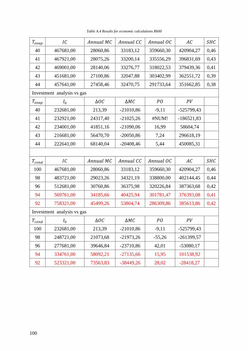
100

Table A.4 Results for economic calculations R600

𝑇𝑇𝑟𝑟𝑣𝑣𝑚𝑚𝑡𝑡 𝐼𝐼𝐶𝐶 𝐴𝐴𝑛𝑛𝑛𝑛𝑢𝑢𝑃𝑃𝑃𝑃 𝑀𝑀𝐶𝐶 𝐴𝐴𝑛𝑛𝑛𝑛𝑢𝑢𝑃𝑃𝑃𝑃 𝐶𝐶𝐶𝐶 𝐴𝐴𝑛𝑛𝑛𝑛𝑢𝑢𝑃𝑃𝑃𝑃 𝑃𝑃𝐶𝐶 𝐴𝐴𝐶𝐶 𝑆𝑆𝑆𝑆𝐶𝐶

40 467681,00 28060,86 33183,12 359660,30 420904,27 0,46

41 467921,00 28075,26 33200,14 335556,29 396831,69 0,43

42 469001,00 28140,06 33276,77 318022,53 379439,36 0,41

43 451681,00 27100,86 32047,88 303402,99 362551,72 0,39

44 457641,00 27458,46 32470,75 291733,64 351662,85 0,38

Investment analysis vs gas

𝑇𝑇𝑟𝑟𝑣𝑣𝑚𝑚𝑡𝑡 𝐼𝐼0 Δ𝑃𝑃𝐶𝐶 Δ𝑀𝑀𝐶𝐶 𝑃𝑃𝑃𝑃 𝑃𝑃𝑉𝑉

40 232681,00 213,39 -21010,86 -9,11 -525799,43

41 232921,00 24317,40 -21025,26 #NUM! -186521,83

42 234001,00 41851,16 -21090,06 16,99 58604,74

43 216681,00 56470,70 -20050,86 7,24 296618,19

44 222641,00 68140,04 -20408,46 5,44 450085,31

𝑇𝑇𝑐𝑐𝑙𝑙𝑐𝑐𝑐𝑐 𝐼𝐼𝐶𝐶 𝐴𝐴𝑛𝑛𝑛𝑛𝑢𝑢𝑃𝑃𝑃𝑃 𝑀𝑀𝐶𝐶 𝐴𝐴𝑛𝑛𝑛𝑛𝑢𝑢𝑃𝑃𝑃𝑃 𝐶𝐶𝐶𝐶 𝐴𝐴𝑛𝑛𝑛𝑛𝑢𝑢𝑃𝑃𝑃𝑃 𝑃𝑃𝐶𝐶 𝐴𝐴𝐶𝐶 𝑆𝑆𝑆𝑆𝐶𝐶

100 467681,00 28060,86 33183,12 359660,30 420904,27 0,46

98 483721,00 29023,26 34321,19 338800,00 402144,45 0,44

96 512681,00 30760,86 36375,98 320226,84 387363,68 0,42

94 569761,00 34185,66 40425,94 301781,47 376393,08 0,41

92 758321,00 45499,26 53804,74 286309,86 385613,86 0,42


𝑇𝑇𝑐𝑐𝑙𝑙𝑐𝑐𝑐𝑐 𝐼𝐼0 Δ𝑃𝑃𝐶𝐶 Δ𝑀𝑀𝐶𝐶 𝑃𝑃𝑃𝑃 𝑃𝑃𝑉𝑉

100 232681,00 213,39 -21010,86 -9,11 -525799,43

98 248721,00 21073,68 -21973,26 -55,26 -261399,57

96 277681,00 39646,84 -23710,86 42,01 -53080,17

94 334761,00 58092,21 -27135,66 15,95 101538,92

92 523321,00 73563,83 -38449,26 28,02 -28418,27

101

Table A.5 Results for economic calculations R600a


40 449676,00 26980,56 31905,62 358518,52 417404,70 0,45

41 449076,00 26944,56 31863,05 342683,75 401491,35 0,43

42 420916,00 25254,96 29865,02 325456,29 380576,28 0,41

43 425116,00 25506,96 30163,02 310825,69 366495,67 0,40

44 431836,00 25910,16 30639,83 299029,13 355579,11 0,38



40 214676,00 1355,17 -19930,56 -9,35 -476476,58

41 214076,00 17189,94 -19894,56 -32,81 -252194,83

42 185916,00 34417,39 -18204,96 17,46 42581,12

43 190116,00 49048,00 -18456,96 7,63 241032,37

44 196836,00 60844,56 -18860,16 5,47 394889,78


100 449676,00 26980,56 31905,62 358518,52 417404,70 0,45

98 465716,00 27942,96 33043,69 338348,87 399335,52 0,43

96 496196,00 29771,76 35206,33 319221,11 384199,19 0,42

94 561636,00 33698,16 39849,45 301781,47 375329,09 0,41

92 781436,00 46886,16 55444,80 285345,31 387676,28 0,42



100 214676,00 1355,17 -19930,56 -9,35 -476476,58

98 230716,00 21524,82 -20892,96 #NUM! -221810,66

96 261196,00 40652,58 -22721,76 26,71 -8480,04

94 326636,00 58092,21 -26648,16 15,02 116534,72

92 546436,00 74528,37 -39836,16 31,75 -57485,88

102

Table A.6 Results for economic calculations R1234ze(Z)


40 497791,00 29867,46 35319,49 343262,41 408449,37 0,44

41 465751,00 27945,06 33046,18 316044,78 377036,01 0,41

42 466831,00 28009,86 33122,81 296845,79 357978,46 0,39

43 449511,00 26970,66 31893,91 280077,16 338941,73 0,37

44 454711,00 27282,66 32262,86 265794,98 325340,50 0,35



40 262791,00 16611,27 -22817,46 -23,30 -350260,66

41 230751,00 43828,91 -20895,06 14,33 92477,38

42 231831,00 63027,89 -20959,86 6,61 361073,48

43 214511,00 79796,53 -19920,66 4,05 629376,16

44 219711,00 94078,71 -20232,66 3,30 821071,07


100 497791,00 29867,46 35319,49 343262,41 408449,37 0,44

98 516791,00 31007,46 36667,59 329785,85 397460,90 0,43

96 549551,00 32973,06 38991,99 308280,25 380245,31 0,41

94 593351,00 35601,06 42099,71 288832,05 366532,83 0,40

92 815271,00 48916,26 57845,48 276421,00 383182,74 0,41



100 262791,00 16611,27 -22817,46 -23,30 -350260,66

98 281791,00 30087,83 -23957,46 #NUM! -195389,89

96 314551,00 51593,43 -25923,06 19,44 47245,76

94 358351,00 71041,63 -28551,06 11,22 240508,73

92 580271,00 83452,69 -41866,26 24,52 5845,82

103

Table A.7 Results sensitivity analysis for R1234ze(Z) for electricity

𝑊𝑊𝑟𝑟𝑙𝑙 = 1,1 NOK/kWh 𝑊𝑊𝑔𝑔𝑚𝑚𝑠𝑠 = 0,37 NOK/kWh

𝑇𝑇𝑟𝑟𝑣𝑣𝑚𝑚𝑡𝑡 𝐴𝐴𝐶𝐶 𝑃𝑃𝑃𝑃 𝑃𝑃𝑉𝑉 𝐺𝐺𝐴𝐴𝑆𝑆 𝐴𝐴𝐶𝐶 40 408449,37 -23,30 -350260,66 383597,51 41 377036,01 14,33 92477,38 383597,51 42 357978,46 6,61 361073,48 383597,51 43 338941,73 4,05 629376,16 383597,51 44 325340,50 3,30 821071,07 383597,51


𝑇𝑇𝑟𝑟𝑣𝑣𝑚𝑚𝑡𝑡 𝐴𝐴𝐶𝐶 𝑃𝑃𝑃𝑃 𝑃𝑃𝑉𝑉 𝐺𝐺𝐴𝐴𝑆𝑆 𝐴𝐴𝐶𝐶 40 346038,02 5,46 529361,41 383597,51 41 319573,33 3,18 902353,30 383597,51 42 304006,50 2,64 1121751,33 383597,51 43 288018,61 2,09 1347083,78 383597,51 44 277014,14 1,93 1502180,10 383597,51


𝑇𝑇𝑟𝑟𝑣𝑣𝑚𝑚𝑡𝑡 𝐴𝐴𝐶𝐶 𝑃𝑃𝑃𝑃 𝑃𝑃𝑉𝑉 𝐺𝐺𝐴𝐴𝑆𝑆 𝐴𝐴𝐶𝐶 40 283626,67 2,41 1408983,49 383597,51 41 262110,64 1,79 1712229,22 383597,51 42 250034,54 1,65 1882429,18 383597,51 43 237095,49 1,41 2064791,41 383597,51 44 228687,78 1,37 2183289,14 383597,51

104

Table A.8 Results sensitivity analysis for R1234ze(Z) for gas price

𝑊𝑊𝑔𝑔𝑚𝑚𝑠𝑠 = 0,35 NOK/kWh 𝑊𝑊𝑟𝑟𝑙𝑙 = 1,1 NOK/kWh

𝑇𝑇𝑟𝑟𝑣𝑣𝑚𝑚𝑡𝑡 𝐴𝐴𝐶𝐶 𝑃𝑃𝑃𝑃 𝑃𝑃𝑉𝑉 𝐺𝐺𝐴𝐴𝑆𝑆 𝐴𝐴𝐶𝐶 40 408449,37 -8,47 -624424,97 364144,88 41 377036,01 #NUM! -181686,93 364144,88 42 357978,46 14,73 86909,17 364144,88 43 338941,73 6,32 355211,85 364144,88 44 325340,50 4,62 546906,76 364144,88


𝑇𝑇𝑟𝑟𝑣𝑣𝑚𝑚𝑡𝑡 𝐴𝐴𝐶𝐶 𝑃𝑃𝑃𝑃 𝑃𝑃𝑉𝑉 𝐺𝐺𝐴𝐴𝑆𝑆 𝐴𝐴𝐶𝐶 40 408449,37 -6,47 -761507,12 354418,56 41 377036,01 -21,45 -318769,08 354418,56 42 357978,46 47,06 -50172,99 354418,56 43 338941,73 8,81 218129,70 354418,56 44 325340,50 5,79 409824,60 354418,56


𝑇𝑇𝑟𝑟𝑣𝑣𝑚𝑚𝑡𝑡 𝐴𝐴𝐶𝐶 𝑃𝑃𝑃𝑃 𝑃𝑃𝑉𝑉 𝐺𝐺𝐴𝐴𝑆𝑆 𝐴𝐴𝐶𝐶 40 408449,37 -5,24 -898589,28 344692,25 41 377036,01 -11,14 -455851,24 344692,25 42 357978,46 #NUM! -187255,14 344692,25 43 338941,73 14,68 81047,54 344692,25 44 325340,50 7,74 272742,44 344692,25

𝑊𝑊𝑔𝑔𝑚𝑚𝑠𝑠 = 0,32 NOK/kWh 𝑊𝑊𝑟𝑟𝑙𝑙 = 1,1 NOK/kWh 𝑇𝑇𝑟𝑟𝑣𝑣𝑚𝑚𝑡𝑡 𝐴𝐴𝐶𝐶 𝑃𝑃𝑃𝑃 𝑃𝑃𝑉𝑉 𝐺𝐺𝐴𝐴𝑆𝑆 𝐴𝐴𝐶𝐶

40 408449,37 -4,40 -1035671,44 334965,93 41 377036,01 -7,60 -592933,39 334965,93 42 357978,46 -20,85 -324337,30 334965,93 43 338941,73 63,05 -56034,61 334965,93 44 325340,50 11,73 135660,29 334965,93

105

Appendix B EES CODE

The code for the EES-model for R600 will follow. R600a has the exactly the same code.

R1234ze(Z) however is different in the SGHE where the inlet values are equal to the outlet

values, since there are no SGHE in that system.

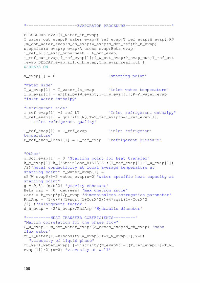
106

"---------------------EVAPORATOR PROCEDURE-------------------" PROCEDURE EVAP(T_water_in_evap; T_water_out_evap;P_water_evap;P_ref_evap;T_ref_evap;W_evap$;R$;m_dot_water_evap;N_ch_evap;W_evap;m_dot_ref;th_m_evap; stepsize;b_evap;p_evap;A_cross_evap;Beta_evap; i_ref_LT;T_evap_superheat : L_out_evap; i_ref_out_evap;i_ref_evap[1];i_w_out_evap;P_evap_out;T_ref_out_evap;DELTAP_evap_all;d_h_evap;T_w_evap_real_out ) $ARRAYS ON y_evap[1] = 0 "starting point" "Water side" T_w_evap[1] = T_water_in_evap "inlet water temperature" i_w_evap[1] = enthalpy(W_evap$;T=T_w_evap[1];P=P_water_evap "inlet water enthalpy" "Refrigerant side" i_ref_evap[1] =i_ref_LT "Inlet refrigerant enthalpy" x_ref_evap[1] = quality(R$;T=T_ref_evap;h=i_ref_evap[1]) "inlet refrigerant quality" T_ref_evap[1] = T_ref_evap "inlet refrigerant temperature" P_ref_evap_local[1] = P_ref_evap "refrigerant pressure" "Other" q_dot_evap[1] = 0 "Starting point for heat transfer" k_m_evap[1]=k_('Stainless_AISI316';(T_ref_evap[1]+T_w_evap[1])/2)"metal conductivity at local average temperature at starting point" c_water_evap[1] = cP(W_evap$;P=P_water_evap;x=0)"water specific heat capacity at starting point" g = 9,81 [m/s^2] "gravity constant" Beta_max = 70 [degrees] "max chevron angle" CorX = b_evap*pi/p_evap "dimensionless corrugation parameter" PhiAmp = (1/6)*((1+sqrt(1+CorX^2))+4*sqrt(1+(CorX^2 /2)))"enlargement factor " d_h_evap = (2*b_evap)/PhiAmp "Hydraulic diameter" "----------HEAT TRANSFER COEFFICIENTS---------" "Martin correlation for one phase flow" G_w_evap = m_dot_water_evap/(A_cross_evap*N_ch_evap) "mass flux water" mu_l_water[1]=viscosity(W_evap$;T=T_w_evap[1];x=0) "viscosity of liquid phase" mu_wall_water_evap[1]=viscosity(W_evap$;T=((T_ref_evap[1]+T_w_evap[1])/2);x=0) "viscosity at wall"

107

Re_w_evap[1] = (G_w_evap*d_h_evap)/mu_l_water[1] "reynolds number" Pr_w[1]=Prandtl(W_evap$;T=T_w_evap[1];x=0)"prandtl number" IF Re_w_evap[1] < 2000 THEN "Parameter for friction factor calculation" f0_martin[1] = 64/Re_w_evap[1] f1_martin[1] = (597/Re_w_evap[1] )+3,85 ELSE f0_martin[1]=(1,8*log10(Re_w_evap[1])-1,5)^(-2) f1_martin[1] = 39/(Re_w_evap[1]^0,289) ENDIF f_martin[1]=(1/(cos(beta_evap)/sqrt(0,18*tan(beta_evap)+0,36*sin(beta_evap)+(f0_martin[1]/cos(beta_evap)))+((1-cos(beta_evap))/(sqrt(3,8*f1_martin[1])))) )^2 "friction factor" Nusselt_w[1]=0,122*(Pr_w[1]^(1/3))*(((mu_l_water[1]/mu_wall_water_evap[1])^(1/6)))*(f_martin[1]*( (Re_w_evap[1]^2)*sin(2*beta_evap)))^0,374"Nusselt number" k_w[1] = conductivity(W_evap$;T=T_w_evap[1];x=0) "water conductivity" h_water_evap[1]=(Nusselt_w[1]*k_w[1])/d_h_evap "heat transfer coefficient water" "General data for refrigerant" rho_g[1] = density(R$;T=T_ref_evap[1];x=1)"density of vapour phase" rho_l[1] = density(R$;T=T_ref_evap[1];x=0)"density of liquid phase" mu_g[1] = viscosity(R$;T=T_ref_evap[1];x=1)"viscosity of vapour phase" mu_l[1] = viscosity(R$;T=T_ref_evap[1];x=0)"viscosity of liquid phase" G_evap= m_dot_ref/(A_cross_evap*N_ch_evap)"mass flux" G_eq[1]=G_evap*((1-x_ref_evap[1])+x_ref_evap[1]*(rho_l[1]/rho_g[1])^0,5) "equivalent mass flux" Re_eq[1]=(G_eq[1]*d_h_evap)/mu_l[1] "equivalent reynolds number" Pr[1]=prandtl(R$;T=T_ref_evap[1];x=0) "prandt number liquid phase" k_ref_evap[1]=Conductivity(R$;T=T_ref_evap[1];x=0)"conductivity refrigerant liquid phase" "Boiling number, X_tt and Bond number" x_m = (1+x_ref_evap[1])/2 "mean quality" rho_m = 1 / ( (x_m/rho_g[1]) + ((1-x_m)/rho_l[1])) "homogenous density"

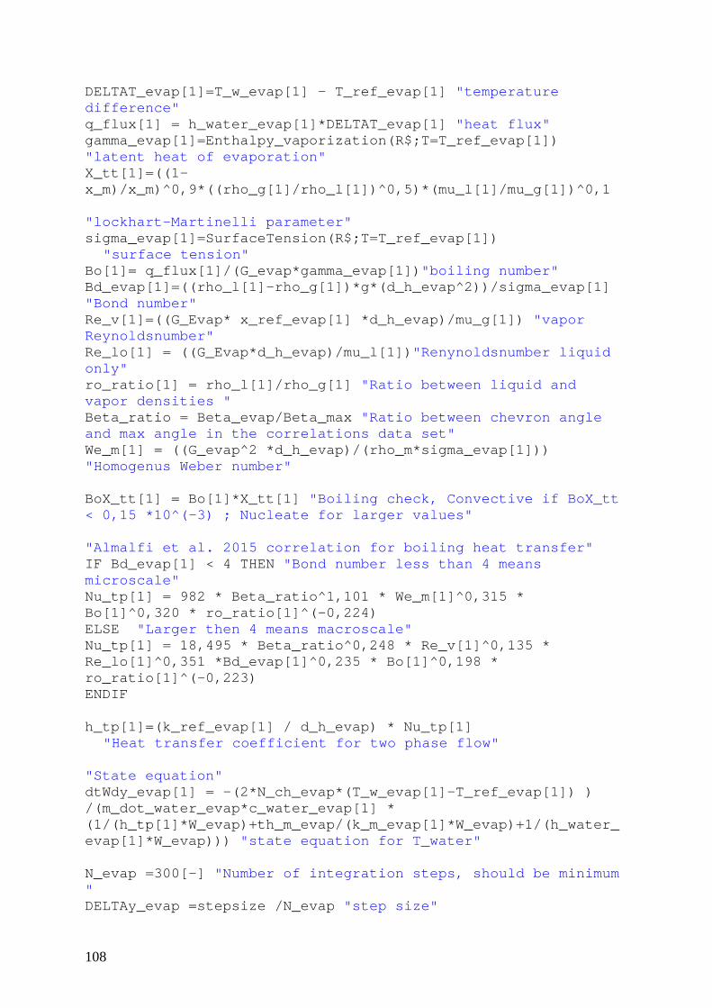
108

DELTAT_evap[1]=T_w_evap[1] - T_ref_evap[1] "temperature difference" q_flux[1] = h_water_evap[1]*DELTAT_evap[1] "heat flux" gamma_evap[1]=Enthalpy_vaporization(R$;T=T_ref_evap[1]) "latent heat of evaporation" X_tt[1]=((1- x_m)/x_m)^0,9*((rho_g[1]/rho_l[1])^0,5)*(mu_l[1]/mu_g[1])^0,1 "lockhart-Martinelli parameter" sigma_evap[1]=SurfaceTension(R$;T=T_ref_evap[1]) "surface tension" Bo[1]= q_flux[1]/(G_evap*gamma_evap[1])"boiling number" Bd_evap[1]=((rho_l[1]-rho_g[1])*g*(d_h_evap^2))/sigma_evap[1] "Bond number" Re_v[1]=((G_Evap* x_ref_evap[1] *d_h_evap)/mu_g[1]) "vapor Reynoldsnumber" Re_lo[1] = ((G_Evap*d_h_evap)/mu_l[1])"Renynoldsnumber liquid only" ro_ratio[1] = rho_l[1]/rho_g[1] "Ratio between liquid and vapor densities " Beta_ratio = Beta_evap/Beta_max "Ratio between chevron angle and max angle in the correlations data set" We_m[1] = ((G_evap^2 *d_h_evap)/(rho_m*sigma_evap[1])) "Homogenus Weber number" BoX_tt[1] = Bo[1]*X_tt[1] "Boiling check, Convective if BoX_tt < 0,15 *10^(-3) ; Nucleate for larger values" "Almalfi et al. 2015 correlation for boiling heat transfer" IF Bd_evap[1] < 4 THEN "Bond number less than 4 means microscale" Nu_tp[1] = 982 * Beta_ratio^1,101 * We_m[1]^0,315 * Bo[1]^0,320 * ro_ratio[1]^(-0,224) ELSE "Larger then 4 means macroscale" Nu_tp[1] = 18,495 * Beta_ratio^0,248 * Re_v[1]^0,135 * Re_lo[1]^0,351 *Bd_evap[1]^0,235 * Bo[1]^0,198 * ro_ratio[1]^(-0,223) ENDIF h_tp[1]=(k_ref_evap[1] / d_h_evap) * Nu_tp[1] "Heat transfer coefficient for two phase flow" "State equation" dtWdy_evap[1] = -(2*N_ch_evap*(T_w_evap[1]-T_ref_evap[1]) ) /(m_dot_water_evap*c_water_evap[1] * (1/(h_tp[1]*W_evap)+th_m_evap/(k_m_evap[1]*W_evap)+1/(h_water_evap[1]*W_evap))) "state equation for T_water" N_evap =300[-] "Number of integration steps, should be minimum " DELTAy_evap =stepsize /N_evap "step size"

109

"Pressure drop" "Amalfi et al 2015 f_tp" C_evap = 2,125*Beta_ratio^9,993 +0,955 "Coefficient for the effect of the corrugation angle in degrees" f_tp[1] =C_evap*15,698*We_m[1]^(-0,475) * Bd_evap[1]^0,255 * ro_ratio[1]^(-0,571) "two phase friction factor Amalfi et al. 2015" DELTAP_evap[1]=(2*f_tp[1]*(G_evap^2)*DELTAy_evap)/(d_h_evap*rho_m) "pressure drop" "-------------------WHILE-LOOP------------------" i = 2 "step variable" REPEAT "While loop for calculating the heatransfer in the two phase region" y_evap[i] = y_evap[i-1] + DELTAy_evap "Heat exchanger location" "Water side" T_w_evap[i] = T_w_evap[i-1] + dtWdy_evap[i-1]*DELTAy_evap "Water temperature" i_w_evap[i] = enthalpy(W_evap$;T=T_w_evap[i];P=P_water_evap) "Water specific enthalpy" q_dot_evap[i] = m_dot_water_evap*(i_w_evap[i-1] - i_w_evap[i])/N_ch_evap "Heat transfered" "Refrigerant side" P_ref_evap_local[i] = P_ref_evap_local[i-1]-DELTAP_evap[i-1] "Refrigerant local pressuret" i_ref_evap[i] = i_ref_evap[i-1] + q_dot_evap[i]/(m_dot_ref/N_ch_evap) "Refrigerant specific enthalpy" x_ref_evap[i] = quality(R$;h=i_ref_evap[i];P=P_ref_evap_local[i]) "Refrigerant quality" "IF ELSE FOR SUPERHEATED VAPOUR temperature change" IF x_ref_evap[i] = 100 THEN T_ref_evap[i] = temperature(R$;P=P_ref_evap_local[i];h=i_ref_evap[i]) ELSE T_ref_evap[i] = temperature(R$;P=P_ref_evap_local[i];x=x_ref_evap[i]) "refrigerant temperature" ENDIF "----------------START OF IF-SENTENCE------------------------"

110

"!If the refrigerant quality is above 0,9, we have to use another correlation" IF (x_ref_evap[i-1] < 0,9) THEN "Two phase region" k_m_evap[i]=k_('Stainless_AISI316';(T_ref_evap[i]+T_w_evap[i])/2) "metal conductivity at local average temperature" c_water_evap[i]=cP(W_evap$;P=P_water_evap;x=0) "specific heat capacity of water" "Martin correlation for one-phase flow water" G_w_evap= m_dot_water_evap/(A_cross_evap*N_ch_evap) "mass flux water" mu_l_water[i]=viscosity(W_evap$;T=T_w_evap[i];x=0) "viscosity of liquid phase" mu_wall_water_evap[i]=viscosity(W_evap$;T=(T_w_evap[i]+T_ref_evap[i])/2;x=0) Re_w_evap[i] = (G_w_evap*d_h_evap)/mu_l_water[i] "reynolds number" Pr_w[i]=Prandtl(W_evap$;T=T_w_evap[i];x=0)"prandtl number" IF Re_w_evap[i] < 2000 THEN "Parameter for friction factor calculation" f0_martin[i] = 64/Re_w_evap[i] f1_martin[i] = (597/Re_w_evap[i])+3,85 ELSE f0_martin[i]=(1,8*log10(Re_w_evap[i])-1,5)^(-2) f1_martin[i]=39/(Re_w_evap[i]^0,289) ENDIF f_martin[i]=(1/(cos(beta_evap)/sqrt(0,18*tan(beta_evap)+0,36*sin(beta_evap)+(f0_martin[i]/cos(beta_evap)))+((1-cos(beta_evap))/(sqrt(3,8*f1_martin[i])))))^2"friction factor" Nusselt_w[i]=0,122*(Pr_w[i]^(1/3))*((mu_l_water[i]/mu_wall_water_evap[i])^(1/6))*(f_martin[i]*((Re_w_evap[i]^2)*sin(2*beta_evap)))^0,374 "Nusselt number" k_w[i] = conductivity(W_evap$;T=T_w_evap[i];x=0) "water conductivity" h_water_evap[i]=(Nusselt_w[i]*k_w[i])/d_h_evap "heat transfer coefficient water" "General data for refrigerant" rho_g[i]= density(R$;T=T_ref_evap[i];x=1)"density of vapor phase" rho_l[i]= density(R$;T=T_ref_evap[i];x=0)"density of liquid phase" mu_g[i] = viscosity(R$;T=T_ref_evap[i];x=1)"viscosity of vapor phase" mu_l[i] = viscosity(R$;T=T_ref_evap[i];x=0) "viscosity of liquid phase"

111

Pr[i]=prandtl(R$;T=T_ref_evap[i];x=0) "prandt number liquid phase" k_ref_evap[i] = Conductivity(R$;T=T_ref_evap[i];x=0) "conductivity refrigerant liquid phase" G_eq[i] = G_evap*((1-x_ref_evap[i])+ x_ref_evap[i]*(rho_l[i]/rho_g[i])^0,5) "equivalent mass flux" Re_eq[i] =(G_eq[i]*d_h_evap)/mu_l[i] "equivalent Reynolds number" "Boiling number and X_tt" DELTAT_evap[i] = T_w_evap[i] - T_ref_evap[i] "Temperature difference" q_flux[i] = h_water_evap[i]*DELTAT_evap[i] "Heat flux" gamma_evap[i]=Enthalpy_vaporization(R$;T=T_ref_evap[i])"latent heat of evaporation" X_tt[i]=((1-x_m)/x_m)^0,9*((rho_g[i]/rho_l[i])^0,5)*(mu_l[i]/mu_g[i])^0,1 "Lockhart-Martinelli parameter" sigma_evap[i]=SurfaceTension(R$;T=T_ref_evap[i]) "surface tension" Bo[i] = q_flux[i]/(G_evap*gamma_evap[i]) "Boiling number" Bd_evap[i] = ((rho_l[i]-rho_g[i])*g*(d_h_evap^2))/ sigma_evap[i] "Bond number" Re_v[i] = ((G_Evap* x_ref_evap[i] *d_h_evap)/mu_g[i]) "vapor Reynoldsnumber" Re_lo[i] = ((G_Evap*d_h_evap)/mu_l[i]) "Renynoldsnumber liquid only" ro_ratio[i] = rho_l[i]/rho_g[i] "Ratio between liquid and vapor densities " Beta_ratio = Beta_evap/Beta_max "Ratio between chevron angle and max angle in the correlations data set" We_m[i]= ((G_evap^2*d_h_evap)/(rho_m*sigma_evap[i]))"Homogenus Weber number" BoX_tt[i] = Bo[i]*X_tt[i] "Boiling check, Convective if BoX_tt < 0,15 *10^(-3) ; Nucleate for larger values" "Almalfi 2015 correlation for boiling heat transfer" IF Bd_evap[i] < 4 THEN "Bond number less than 4 means microscale" Nu_tp[i] = 982 * Beta_ratio^1,101 * We_m[i]^0,315 * Bo[i]^0,320 * ro_ratio[i]^(-0,224) ELSE "Larger then 4 means macroscale" Nu_tp[i] = 18,495 * Beta_ratio^0,248 * Re_v[i]^0,135 * Re_lo[i]^0,351 *Bd_evap[i]^0,235 * Bo[i]^0,198 * ro_ratio[i]^(-0,223) ENDIF h_tp[i]=(k_ref_evap[i] / d_h_evap) * Nu_tp[i] "Heat transfer coefficient for twophase flow"

112

h_dummy = max(h_tp[i])"dummy variable which saves the heat transfer coefficient. To be used later for the linear equation" "State equation for T_water, to calculate temperature change" dtWdy_evap[i] = -(2*N_ch_evap*(T_w_evap[i]-T_ref_evap[i]) ) /(m_dot_water_evap*c_water_evap[i] * (1/(h_tp[i]*W_evap)+th_m_evap/(k_m_evap[i]*W_evap)+1/(h_water_evap[i]*W_evap))) "Pressure drop" f_tp[i] =C_evap*15,698*We_m[i]^(-0,475) * Bd_evap[i]^0,255 * ro_ratio[i]^(-0,571) "two phase friction factor" DELTAP_evap[i]=(2*f_tp[i-1]*(G_evap^2)*DELTAy_evap)/(d_h_evap*rho_m) "pressure drop" DELTAP_evap_tot[1] = 0 "initializing array" DELTAP_evap_tot[i] = DELTAP_evap_tot[i-1] + DELTAP_evap[i] "pressure drop" i = i +1 "counter" ELSE "If quality is higher than 0,9" "----------HEAT TRANSFER COEFFICIENTS---------" y_evap[i] = y_evap[i-1] + DELTAy_evap "Heat exchanger location" "Water side" T_w_evap[i] = T_w_evap[i-1] + dtWdy_evap[i-1]*DELTAy_evap "Water temperature" i_w_evap[i] = enthalpy(W_evap$;T=T_w_evap[i];P=P_water_evap) "Water specific enthalpy" q_dot_evap[i] = m_dot_water_evap*(i_w_evap[i-1] - i_w_evap[i])/N_ch_evap "Heat transfered" "Refrigerant side" P_ref_evap_local[i] = P_ref_evap_local[i-1]-DELTAP_evap[i-1] "pressure of refrigerant" i_ref_evap[i]=i_ref_evap[i-1] + q_dot_evap[i]/(m_dot_ref/N_ch_evap) "Refrigerant specific enthalpy" x_ref_evap[i]=quality(R$;h=i_ref_evap[i];P=P_ref_evap_local[i]) "Refrigerant quality" IF (x_ref_evap[i] = 100) THEN "if else sentence to give the correct temperature while transitioning" T_ref_evap[i] = T_ref_evap[i-1] ELSE

113

T_ref_evap[i]=temperature(R$;P=P_ref_evap_local[i];x=x_ref_evap[i]) "refrigerant temperature" ENDIF "Martin correlation for one-phase flow water" G_w_evap= m_dot_water_evap/(A_cross_evap*N_ch_evap) "mass flux water" mu_l_water[i]=viscosity(W_evap$;T=T_w_evap[i];x=0) "viscosity of liquid phase" mu_wall_water_evap[i]=viscosity(W_evap$;T=(T_w_evap[i]+T_ref_evap[i])/2;x=0) Re_w_evap[i]=(G_w_evap*d_h_evap)/mu_l_water[i] "reynolds number" Pr_w[i]=Prandtl(W_evap$;T=T_w_evap[i];x=0)"prandtl number" IF Re_w_evap[i] < 2000 THEN "Parameter for friction factor calculation" f0_martin[i] = 64/Re_w_evap[i] f1_martin[i] = (597/Re_w_evap[i] )+3,85 ELSE f0_martin[i] =(1,8*log10(Re_w_evap[i])-1,5)^(-2) f1_martin[i]= 39/(Re_w_evap[i]^0,289) ENDIF f_martin[i]=(1/(cos(beta_evap)/sqrt(0,18*tan(beta_evap)+0,36*sin(beta_evap)+(f0_martin[i]/cos(beta_evap))) + ((1-cos(beta_evap))/(sqrt(3,8*f1_martin[i])))))^2 "friction factor" Nusselt_w[i]=0,122*(Pr_w[i]^(1/3))*(((mu_l_water[i]/mu_wall_water_evap[i])^(1/6)))*(f_martin[i]*((Re_w_evap[i]^2)*sin(2*beta_evap)))^0,374 "Nusselt number" k_w[i] = conductivity(W_evap$;T=T_w_evap[i];x=0) "water conductivity" h_water_evap[i]=(Nusselt_w[i]*k_w[i])/d_h_evap "heat transfer coefficient water" "Two-phase heat transfer coefficient" "Linear correlation for wall dry out" y_1 = h_dummy y_2 = 600 x_1 = 0,9 x_2 = 1,0 a = (y_2-y_1)/(x_2-x_1) b = y_2 -a*x_2 IF (x_ref_evap[i] < 100) THEN "if sentence to correctly transition between correlations" h_tp[i] = a*x_ref_evap[i] + b ELSE h_tp[i] = h_tp[i-1] ENDIF

114

"Boiling number check" rho_g[i] = density(R$;T=T_ref_evap[i];x=1)"density of vapour phase" rho_l[i] = density(R$;T=T_ref_evap[i];x=0)"density of liquid phase" mu_g[i] = viscosity(R$;T=T_ref_evap[i];x=1)"viscosity of vapour phase" mu_l[i] = viscosity(R$;T=T_ref_evap[i];x=0)"viscosity of liquid phase" Pr[i]=prandtl(R$;T=T_ref_evap[i];x=0)"prandt number liquid phase" k_ref_evap[i]= Conductivity(R$;T=T_ref_evap[i];x=0) "conductivity refrigerant liquid phase" IF (x_ref_evap[i] < 100) THEN "if else to prevent error given by x less than zero" G_eq[i]=G_evap*((1-x_ref_evap[i])+ x_ref_evap[i]*(rho_l[i]/rho_g[i])^0,5) "equivalent mass flux" ELSE G_eq[i] = G_eq[i-1] ENDIF Re_eq[i] = (G_eq[i]*d_h_evap)/mu_l[i] "equivalent reynolds number" gamma_evap[i]=Enthalpy_vaporization(R$;T=T_ref_evap[i])"latent heat of evaporation" X_tt[i] = ((1-x_m)/x_m)^0,9* ((rho_g[i]/rho_l[i])^0,5)*(mu_l[i]/mu_g[i])^0,1 "Lockhart-Martinelli parameter" "Boiling number and X_tt" DELTAT_evap[i] = T_w_evap[i] - T_ref_evap[i] "Temperature difference" q_flux[i] = h_water_evap[i]*DELTAT_evap[i] "Heat flux" Bo[i] = q_flux[i]/(G_evap*gamma_evap[i])"Boiling number" BoX_tt[i] = Bo[i]*X_tt[i] "convective boiling check" "Misc" k_m_evap[i]=k_('Stainless_AISI316';(T_ref_evap[i]+T_w_evap[i])/2) "metal conductivity at local average temperature" c_water_evap[i] = cP(W_evap$; P=P_water_evap;x=0)" specific heat capacity of water" "State equation for T_water, to calculate temperature change" dtWdy_evap[i] = -(2*N_ch_evap*(T_w_evap[i]-T_ref_evap)) /(m_dot_water_evap*c_water_evap[i] * (1/(h_tp[i]*W_evap)+th_m_evap/(k_m_evap[i]*W_evap)+1/(h_water_evap[i]*W_evap))) "Pressure drop"

115

sigma_evap[i]=SurfaceTension(R$;T=T_ref_evap[i]) "surface tension" Bd_evap[i] = ((rho_l[i]-rho_g[i])*g*(d_h_evap^2))/sigma_evap[i] "Bond number" f_tp[i]=C_evap*15,698*((((G_evap^2*d_h_evap)/(rho_m*sigma_evap[i]))^(-0,475))*(Bd_evap[i]^0,255)*((rho_l[i]/rho_g[i])^(-0,571))) "two phase friction factor" DELTAP_evap[i]=(2*f_tp[i-1]*(G_evap^2)*DELTAy_evap) /(d_h_evap*rho_m) "pressure drop" DELTAP_evap_tot[i] = DELTAP_evap_tot[i-1] + DELTAP_evap[i] "cumulative pressure drop" i = i+1 "counter" ENDIF UNTIL ( x_ref_evap[i-1] = 100) "End condition, saturated vapour" "---------------While loop for superheated part--------------" REPEAT y_evap[i] = y_evap[i-1] + DELTAy_evap "Heat exchanger location" L_out_evap = y_evap[i] "Final length of heat exchanger" "Water side" T_w_evap[i] = T_w_evap[i-1] + dtWdy_evap[i-1]*DELTAy_evap "Water temperature" i_w_evap[i] = enthalpy(W_evap$;T=T_w_evap[i];P=P_water_evap) "Water specific enthalpy" {i_w_out_evap = i_w_evap[i-1] "water outlet enthalpy"} i_w_out_evap = i_w_evap[i] "water outlet enthalpy" q_dot_evap[i] = m_dot_water_evap*(i_w_evap[i-1]- i_w_evap[i])/N_ch_evap "Heat transfered" T_w_evap_real_out = T_w_evap[i] "Outlet water tempeature" "Refrigerant side" P_ref_evap_local[i] = P_ref_evap_local[i-1]-DELTAP_evap[i-1] "pressure of refrigerant" i_ref_evap[i] = i_ref_evap[i-1] + q_dot_evap[i]/(m_dot_ref/N_ch_evap)"Refrigerant specific enthalpy" T_ref_evap[i]=temperature(R$;P=P_ref_evap_local[i];h=i_ref_evap[i]) "Temperature refrigerant" T_ref_out_evap = T_ref_evap[i] "Refrigerant outlet temperature" i_ref_out_evap = i_ref_evap[i] "specific enthalpy of refrigerant out of the evaporator" "Martin correlation for one-phase flow water"

116

G_w_evap= m_dot_water_evap/(A_cross_evap*N_ch_evap) "mass flux water" mu_l_water[i]=viscosity(W_evap$;T=T_w_evap[i];x=0) "viscosity of liquid phase" mu_wall_water_evap[i]=viscosity(W_evap$;T=(T_w_evap[i]+T_ref_evap[i])/2;x=0) "viscosity at wall" Re_w_evap[i]=(G_w_evap*d_h_evap)/mu_l_water[i] "reynolds number" Pr_w[i]=Prandtl(W_evap$;T=T_w_evap[i];x=0) "prandtl number" IF Re_w_evap[i] < 2000 THEN "Parameter for friction factor calculation" f0_martin[i] = 64/Re_w_evap[i] f1_martin[i] = (597/Re_w_evap[i] )+3,85 ELSE f0_martin[i] = (1,8*log10(Re_w_evap[i])-1,5)^(-2) f1_martin[i]=39/(Re_w_evap[i]^0,289) ENDIF f_martin[i]=(1/(cos(beta_evap)/sqrt(0,18*tan(beta_evap)+0,36*sin(beta_evap)+(f0_martin[i]/cos(beta_evap))) + ((1-cos(beta_evap))/(sqrt(3,8*f1_martin[i])))) )^2 "friction factor" Nusselt_w[i]=0,122*(Pr_w[i]^(1/3))*(((mu_l_water[i]/mu_wall_water_evap[i])^(1/6)))*(f_martin[i]*( (Re_w_evap[i]^2)*sin(2*beta_evap)))^0,374 "Nusselt number" k_w[i] = conductivity(W_evap$;T=T_w_evap[i];x=0) "water conductivity" h_water_evap[i]=(Nusselt_w[i]*k_w[i])/d_h_evap "heat transfer coefficient water" "Martin correlation for one-phase flow refrigerant" rho_g[i] = density(R$;T=T_ref_evap[i];x=1)"density of vapour phase" rho_l[i] = density(R$;T=T_ref_evap[i];x=0)"density of liquid phase" mu_g[i] = viscosity(R$;T=T_ref_evap[i];x=1)"viscosity of vapour phase" mu_l[i] = viscosity(R$;T=T_ref_evap[i];x=0)"viscosity of liquid phase" Pr[i]=prandtl(R$;T=T_ref_evap[i];x=0) "prandt number liquid phase" G_ref_evap=m_dot_ref/(A_cross_evap*N_ch_evap) "mass flux refrigerant" mu_wall_ref_evap[i]=viscosity(R$;T=(T_ref_evap[i]+T_w_evap[i])/2;x=1) "Viscosity at wall" Re_ref_evap[i] =(G_ref_evap*d_h_evap)/mu_g[i]"reynolds number" Pr_ref_evap[i]=Prandtl(R$;T=T_ref_evap[i];x=1)"prandtl number"

117

IF Re_ref_evap[i] < 2000 THEN "Parameter for friction factor calculation" f0_martin_ref_evap[i] = 64/Re_ref_evap[i] f1_martin_ref_evap[i]= (597/Re_ref_evap[i] )+3,85 ELSE f0_martin_ref_evap[i] =(1,8*log10(Re_ref_evap[i])-1,5)^(-2) f1_martin_ref_evap[i]=39/(Re_ref_evap[i]^0,289) ENDIF f_martin_ref_evap[i]=(1/(cos(Beta_evap)/sqrt(0,18*tan(Beta_evap)+0,36*sin(Beta_evap)+(f0_martin_ref_evap[i]/cos(Beta_evap))) + ((1-cos(Beta_evap))/(sqrt(3,8*f1_martin_ref_evap[i])))) )^2 "friction factor" Nusselt_ref_evap[i]=0,122*(Pr[i]^(1/3))*((mu_g[i]/mu_wall_ref_evap[i])^(1/6))*(f_martin_ref_evap[i]*((Re_ref_evap[i]^2)*sin(2*Beta_evap)))^0,374 "Nusselt number" k_ref_evap[i] = conductivity(R$;T=T_ref_evap[i];x=1) "refrigerant conductivity" h_ref[i]=(Nusselt_ref_evap[i]*k_ref_evap[i])/d_h_evap "heat transfer coefficient" "Misc" k_m_evap[i]=k_('Stainless_AISI316';(T_ref_evap[i]+T_w_evap[i])/2) "metal conductivity at local average temperature" c_water_evap[i] = cP(W_evap$; P=P_water_evap;x=0)"specific heat capacity of water" "State equation for T_water, to calculate temperature change" dtWdy_evap[i] = -(2*N_ch_evap*(T_w_evap[i]-T_ref_evap)) /(m_dot_water_evap*c_water_evap[i] * (1/(h_ref[i]*W_evap)+th_m_evap/(k_m_evap[i]*W_evap)+1/(h_water_evap[i]*W_evap))) "Misc pressure drops except the frictional pressure drop" DELTAP_evap[i]=(2*f_martin_ref_evap[i]*(G_ref_evap^2)*DELTAy_evap)/(d_h_evap*rho_g[i]) "pressure drop" DELTAP_evap_tot[i] = DELTAP_evap_tot[i-1] + DELTAP_evap[i] "cumulative pressure drop" g = 9,81 [m/s^2] "gravitational constant" DELTAPgravity_evap = rho_m*g*L_out_evap "gravity driven acceleration" DELTAx_ref_evap = abs(1 - x_ref_evap[1])"quality change" DELTAPacc_evap = (G_evap^2)*DELTAx_ref_evap*( (1/rho_g[1]) - (1/rho_l[1])) "acceleration pressure" DELTAPmanifold_evap = 1,5*(rho_m*((G_evap/rho_m)^2)*0,5) "inlet/outlet pressure loss"

118

DELTAP_evap_all = DELTAP_evap_tot[i] + DELTAPgravity_evap + DELTAPacc_evap + DELTAPmanifold_evap "total pressure loss" P_evap_out =P_ref_evap - DELTAP_evap_all "outlet pressure" i = i +1 i_ref_evap_needed = enthalpy(R$;T=T_ref_evap + T_evap_superheat;P=P_ref_evap) "needed rerigerant enthalpy to reach the correct superheat temperature" UNTIL ( i_ref_evap[i-1] > i_ref_evap_needed) "End condition" END "--------------END OF EVAPORATOR PROCEDURE-------------------" "---------------------CONDENSER PROCEDURE---------------------" PROCEDURE COND(T_water_in_cond;P_water_cond;P_ref_cond;T_ref_cond;T_water_out_cond;W_cond$;R$;m_dot_water_cond;W_cond;m_dot_ref;th_m_cond; stepsize;h_condenser_inlet; N_ch_cond;b_cond;A_cross_cond;beta_cond;p_cond;T_condenser_inlet;T_subcool : i_ref_out_cond;x_ref_out_cond;T_w_real_out;L_out_cond;i_w_out_cond;P_cond_out;T_ref_cond_out;d_h_cond) $ARRAYS ON "----DESUPERHEATER PART--------------------------------------" "Initializing variables, starting points" y_cond[1] = 0 "Starting point" "Water side" T_w_cond[1] = T_water_in_cond "Inlet water temperature" i_w_cond[1] =enthalpy(W_cond$;T=T_w_cond[1];P=P_water_cond) "Inlet water enthalpy" i_w_out_wanted_cond=enthalpy(W_cond$;T=T_water_out_cond;P=P_water_cond)"wanted outlet enthalpy" "Refrigerant side" i_ref_cond[1] = h_condenser_inlet "Inlet refrigerant enthalpy" T_ref_cond[1] = T_condenser_inlet "Inlet refrigerant temperature" P_ref_cond_local[1] = P_ref_cond "local refrigerant pressure" x_ref_cond[1]=quality(R$;h=i_ref_cond[1];P=P_ref_cond_local[1])"refrigerant quality" "Other" q_dot_cond[1] = 0 "Starting point for heat transfer"

119

k_m_cond[1]=k_('Stainless_AISI316';(T_ref_cond+T_w_cond[1])/2)"Metal conductivity at local average temperature at starting point" phi = 1,20"Longo 2015 enlargement factor beta 45" {phi = 1,24}"Longo 2015 for Beta 65" c_water_cond[1] = cP(W_cond$; P=P_water_cond;x=0) "Water specific heat capacity at starting point" N_cond = 300 [-]"Number of integration steps" DELTAy_cond = stepsize/N_cond "step size" CorX = b_cond*pi/p_cond "dimensionless corrugation parameter" PhiAmp = (1/6)*((1+sqrt(1+CorX^2))+4*sqrt(1+(CorX^2 /2))) "enlargement factor " d_h_cond = (2*b_cond)/PhiAmp "Hydraulic diameter" "Variables related to pressure drop" rho_g_cond[1] = density(R$;T=T_ref_cond[1];x=1) "density of vapour phase" rho_l_cond[1] = density(R$;T=T_ref_cond[1];x=0) "density of liquid phase" rho_m_cond = (rho_g_cond[1]+rho_l_cond[1])/2 "mean density" "----------HEAT TRANSFER COEFFICIENTS---------" "Martin correlation for one-phase flow" G_w_cond = m_dot_water_cond/(A_cross_cond*N_ch_cond)"mass flux water" mu_l_water_cond[1] = viscosity(W_cond$;T=T_w_cond[1];x=0) "viscosity of liquid phase" mu_wall_water_cond[1]=viscosity(W_cond$;T=(T_w_cond[1]+T_ref_cond[1])/2;x=0) "viscosity at wall" Re_w_cond[1] =(G_w_cond*d_h_cond)/mu_l_water_cond[1]"reynolds number" Pr_w_cond[1]=Prandtl(W_cond$;T=T_w_cond[1];x=0)"prandtl number" IF Re_w_cond[1] < 2000 THEN "Parameter for friction factor calculation" f0_martin_cond[1]= 64/Re_w_cond[1] f1_martin_cond[1]= (597/Re_w_cond[1] )+3,85 ELSE f0_martin_cond[1]= (1,8*log10(Re_w_cond[1])-1,5)^(-2) f1_martin_cond[1]=39/(Re_w_cond[1]^0,289) ENDIF f_martin_cond[1]=(1/(cos(Beta_cond)/sqrt(0,18*tan(Beta_cond)+0,36*sin(Beta_cond)+(f0_martin_cond[1]/cos(Beta_cond))) + ((1-cos(Beta_cond))/(sqrt(3,8*f1_martin_cond[1])))) )^2 "friction factor"

120

Nusselt_w_cond[1]=0,122*(Pr_w_cond[1]^(1/3))*((mu_l_water_cond[1]/mu_wall_water_cond[1])^(1/6))*(f_martin_cond[1]*((Re_w_cond[1]^2)*sin(2*Beta_cond)))^0,374 "Nusselt number. Should also include the viscosity term later" k_w_cond[1] = conductivity(W_cond$;T=T_w_cond[1];x=0)"water conductivity" h_water_cond[1] =(Nusselt_w_cond[1]*k_w_cond[1])/d_h_cond "heat transfer coefficient water" IF (x_ref_cond[1] = 100) THEN "SUPERHEATED VAPOUR" "Martin correlation for one-phase flow refrigerant" G_ref_cond=m_dot_ref/(A_cross_cond*N_ch_cond) "mass flux refrigerant" mu_g_ref_cond[1]=viscosity(R$;T=T_ref_cond[1];x=1) "viscosity of liquid phase" mu_wall_ref_cond[1]=viscosity(R$;T=(T_ref_cond[1]+T_w_cond[1])/2;x=1) "viscosity at wall" Re_ref_cond[1] =(G_ref_cond*d_h_cond)/mu_g_ref_cond[1]"reynolds number" Pr_ref_cond[1]=Prandtl(R$;T=T_ref_cond[1];x=1)"prandtl number" IF Re_ref_cond[1] < 2000 THEN "Parameter for friction factor calculation" f0_martin_ref_cond[1] = 64/Re_ref_cond[1] f1_martin_ref_cond[1]= (597/Re_ref_cond[1] )+3,85 ELSE f0_martin_ref_cond[1] = (1,8*log10(Re_ref_cond[1])-1,5)^(-2) f1_martin_ref_cond[1]=39/(Re_ref_cond[1]^0,289) ENDIF f_martin_ref_cond[1]=(1/(cos(Beta_cond)/sqrt(0,18*tan(Beta_cond)+0,36*sin(Beta_cond)+(f0_martin_ref_cond[1]/cos(Beta_cond))) + ((1-cos(Beta_cond))/(sqrt(3,8*f1_martin_ref_cond[1])))))^2 "friction factor" Nusselt_ref_cond[1]=0,122*(Pr_ref_cond[1]^(1/3))*((mu_g_ref_cond[1]/mu_wall_ref_cond[1])^(1/6))*(f_martin_ref_cond[1]*( (Re_ref_cond[1]^2)*sin(2*Beta_cond)))^0,374 "Nusselt number. Should also include the viscosity term" k_ref_cond[1] = conductivity(R$;T=T_ref_cond[1];x=1) "Refrigerant conductivity" h_ref_cond[1] = (Nusselt_ref_cond[1]*k_ref_cond[1])/d_h_cond "heat transfer coefficient ref" {DELTAP_cond[1]=(2*f_martin_ref_cond[1]*(G_ref_cond^2)*DELTAy_cond)/(d_h_cond*rho_m_cond) DELTAP_cond_tot[1] = 0} "total pressure drop" ELSE "Incase of no superheated vapor at starting conditions" "Longo 2015 correlation for condensation of saturated gas"

121

G_ref_cond = m_dot_ref/(A_cross_cond*N_ch_cond)"mass flux" rho_g_cond[1] = density(R$;T=T_ref_cond[1];x=1)"density of vapor phase" rho_l_cond[1] = density(R$;T=T_ref_cond[1];x=0)"density of liquid phase" G_eq_cond[1] = G_ref_cond *((1-x_ref_cond[1] )+ x_ref_cond[1] *(rho_l_cond[1]/rho_g_cond[1])^0,5)"equivalent mass flux" mu_l_cond[1]=viscosity(R$;T=T_ref_cond[1];x=0)"viscosity of liquid phase" Re_eq_cond[1] =(G_eq_cond[1]*d_h_cond)/mu_l_cond[1]"equivalent reynolds number" Pr_l_cond[1]=Prandtl(R$;T=T_ref_cond[1];x=0)"prandtl number liquid phase" k_ref_cond[1]=conductivity(R$;T=T_ref_cond[1];x=0)"conductivity refrigerant" h_ref_cond[1]=1,875*phi*(k_ref_cond[1]/d_h_cond)*(Re_eq_cond[1]^0,445)*(Pr_l_cond[1]^(1/3)) "two phase heat trans coeff" ENDIF "State equation for T_water" dtWdy_cond[1] = (2*N_ch_cond*(T_ref_cond[1]-T_w_cond[1]) ) /(m_dot_water_cond*c_water_cond[1]*(1/(h_ref_cond[1]*W_cond)+th_m_cond/(k_m_cond[1]*W_cond)+1/(h_water_cond[1]*W_cond))) i = 2 "step counter" REPEAT y_cond[i] = y_cond[i-1] +DELTAy_cond "Location in heat exchanger" L_out_cond = y_cond[i] "plate length" "Water side" T_w_cond[i] = T_w_cond[i-1] + dtWdy_cond[i-1]*DELTAy_cond "Water temperature" i_w_cond[i] = enthalpy(W_cond$;T=T_w_cond[i];P=P_water_cond) "Water specific enthalpy" q_dot_cond[i] = m_dot_water_cond*(i_w_cond[i-1] - i_w_cond[i])/N_ch_cond "Heat transfered" T_w_real_out = T_w_cond[i-1]"Water temperature at outlet" i_w_out_cond =i_w_cond[i-1]"water enthalpy at outlet" "Refrigerant side" P_ref_cond_local[i] = P_ref_cond "P_ref_cond_local[i-1] - DELTAP_cond[i-1]" "local pressure" i_ref_cond[i]=i_ref_cond[i-1]+q_dot_cond[i]/ (m_dot_ref/N_ch_cond) "Refrigerant specific enthalpy" x_ref_cond[i]=quality(R$;h=i_ref_cond[i];P=P_ref_cond_local[i]) "Refrigerant quality"

122

"--------------------START OF IF SENTENCE-------------------" IF (x_ref_cond[i] = 100) THEN "If superheated vapour" T_ref_cond[i]=temperature(R$;P=P_ref_cond_local[i];h=i_ref_cond[i])"Refrigerant temperature" T_ref_cond_out =T_ref_cond[i-1] "outlet temperature of refrigerant" i_ref_out_cond = i_ref_cond[i-1] "refrigerant enthalpy at condenser outlet" x_ref_out_cond = x_ref_cond[i-1] "refrigerant quality at condenser outlet" c_water_cond[i] = cP(W_cond$; T=T_ref_cond[i];P=P_ref_cond_local[i])"Specific heat capacity water" c_water_cond1[i]= cP(W_cond$; T=T_ref_cond[i];x=0) "Specific heat liquid water" k_m_cond[i]=k_('Stainless_AISI316';(T_ref_cond+T_w_cond[i])/2) "Metal conductivity at local average temperature" "----------HEAT TRANSFER COEFFICIENTS---------" "Martin correlation water side" G_w_cond = m_dot_water_cond/(A_cross_cond*N_ch_cond) "mass flux water" mu_l_water_cond[i] =viscosity(W_cond$;T=T_w_cond[i];x=0) "viscosity of liquid phase" mu_wall_water_cond[i]=viscosity(W_cond$;T=(T_w_cond[i]+T_ref_cond[i])/2;x=0) "viscosity at wall" Re_w_cond[i] = (G_w_cond*d_h_cond)/mu_l_water_cond[i]"reynolds number" Pr_w_cond[i]=Prandtl(W_cond$;T=T_w_cond[i];x=0) "prandtl number" IF Re_w_cond[i] < 2000 THEN "Parameter for friction factor calculation" f0_martin_cond[i] = 64/Re_w_cond[i] f1_martin_cond[i]= (597/Re_w_cond[i])+3,85 ELSE f0_martin_cond[i]= (1,8*log10(Re_w_cond[i])-1,5)^(-2) f1_martin_cond[i]=39/(Re_w_cond[i]^0,289) ENDIF f_martin_cond[i]=(1/(cos(Beta_cond)/sqrt(0,18*tan(Beta_cond)+0,36*sin(Beta_cond)+(f0_martin_cond[i]/cos(Beta_cond))) + ((1-cos(Beta_cond))/(sqrt(3,8*f1_martin_cond[i])))) )^2 "friction factor"

123

Nusselt_w_cond[i]=0,122*(Pr_w_cond[i]^(1/3))*((mu_l_water_cond[i]/mu_wall_water_cond[i])^(1/6))*(f_martin_cond[i]*((Re_w_cond[i]^2)*sin(2*Beta_cond)))^0,374 "Nusselt number. Should also include the viscosity term" k_w_cond[i] = conductivity(W_cond$;T=T_w_cond[i];x=0) "water conductivity" h_water_cond[i] =(Nusselt_w_cond[i]*k_w_cond[i])/d_h_cond "heat transfer coefficient water" "Martin correlation refrigerant side" G_ref_cond =m_dot_ref/(A_cross_cond*N_ch_cond)"mass flux refrigerant" mu_g_ref_cond[i] =viscosity(R$;T=T_ref_cond[i];x=1) "viscosity of gas phase" mu_wall_ref_cond[i]=viscosity(R$;T=((T_ref_cond[i]+T_w_cond[i])/2);x=1)"viscosity at wall" Re_ref_cond[i]=(G_ref_cond*d_h_cond)/mu_g_ref_cond[i]"reynolds number" Pr_ref_cond[i]=Prandtl(R$;T=T_ref_cond[i];x=1)"prandtl number" IF Re_ref_cond[i] < 2000 THEN "Parameter for friction factor calculation" f0_martin_ref_cond[i] = 64/Re_ref_cond[i] f1_martin_ref_cond[i]= (597/Re_ref_cond[i] )+3,85 ELSE f0_martin_ref_cond[i]=(1,8*log10(Re_ref_cond[i])-1,5)^(-2) f1_martin_ref_cond[i]=39/(Re_ref_cond[i]^0,289) ENDIF f_martin_ref_cond[i]=(1/(cos(Beta_cond)/sqrt(0,18*tan(Beta_cond)+0,36*sin(Beta_cond)+(f0_martin_ref_cond[i]/cos(Beta_cond))) + ((1-cos(Beta_cond))/(sqrt(3,8*f1_martin_ref_cond[i])))) )^2 "friction factor" Nusselt_ref_cond[i]=0,122*(Pr_ref_cond[i]^(1/3))*((mu_g_ref_cond[i]/mu_wall_ref_cond[i])^(1/6))*(f_martin_ref_cond[i]*((Re_ref_cond[i]^2)*sin(2*Beta_cond)))^0,374 "Nusselt number. " k_ref_cond[i] = conductivity(R$;T=T_ref_cond[i];x=1) "Refrigerant conductivity" h_ref_cond[i]=(Nusselt_ref_cond[i]*k_ref_cond[i])/d_h_cond "heat transfer coefficient water" "Pressure drop" {DELTAP_cond[i]=(2*f_martin_ref_cond[i]*(G_ref_cond^2)*DELTAy_cond)/(d_h_cond*rho_m_cond) DELTAP_cond_tot[i] = DELTAP_cond_tot[i-1] + DELTAP_cond[i]} "State equation for T_water" dtWdy_cond[i] = (2*N_ch_cond*(T_ref_cond-T_w_cond[i]) ) /(m_dot_water_cond*c_water_cond[i] * (1/(h_ref_cond[i]*W_cond)+th_m_cond/(k_m_cond[i]*W_cond)+1/(h_water_cond[i]*W_cond))) i = i + 1

124

ELSE "CONDENSING SECTION" T_ref_cond[i]=temperature(R$;P=P_ref_cond_local[i];h=i_ref_cond[i]) "refrigerant temperature" T_ref_cond_out =T_ref_cond[i-1]"outlet temperature of rerigerant" i_ref_out_cond = i_ref_cond[i-1]"refrigerant enthalpy at condenser outlet" x_ref_out_cond = x_ref_cond[i-1]"refrigerant quality at condenser outlet" c_water_cond[i] = cP(W_cond$; P=P_water_cond;T=T_w_cond[i]) "Specific heat capacity water" k_m_cond[i] = k_('Stainless_AISI316';(T_ref_cond[i]+T_w_cond[i])/2) "Metal conductivity at local average temperature" "----------HEAT TRANSFER COEFFICIENTS---------" "Martin correlation one phase flow" G_w_cond = m_dot_water_cond/(A_cross_cond*N_ch_cond) "mass flux water" mu_l_water_cond[i] =viscosity(W_cond$;T=T_w_cond[i];x=0) "viscosity of liquid phase" mu_wall_water_cond[i]=viscosity(W_cond$;T=((T_w_cond[i]+T_ref_cond[i])/2);x=0) "viscosity gas phase" Re_w_cond[i] = (G_w_cond*d_h_cond)/mu_l_water_cond[i] "reynolds number" Pr_w_cond[i]=Prandtl(W_cond$;T=T_w_cond[i];x=0) "prandtl number" IF Re_w_cond[i] < 2000 THEN "Parameter for friction factor calculation" f0_martin_cond[i] = 64/Re_w_cond[i] f1_martin_cond[i]= (597/Re_w_cond[i] )+3,85 ELSE f0_martin_cond[i]= (1,8*log10(Re_w_cond[i])-1,5)^(-2) f1_martin_cond[i]=39/(Re_w_cond[i]^0,289) ENDIF f_martin_cond[i]=(1/(cos(Beta_cond)/sqrt(0,18*tan(Beta_cond)+0,36*sin(Beta_cond)+(f0_martin_cond[i]/cos(Beta_cond))) + ((1-cos(Beta_cond))/(sqrt(3,8*f1_martin_cond[i])))))^2 "friction factor" Nusselt_w_cond[i]=0,122*(Pr_w_cond[i]^(1/3))*((mu_l_water_cond[i]/mu_wall_water_cond[i])^(1/6))*(f_martin_cond[i]*((Re_w_cond[i]^2)*sin(2*Beta_cond)))^0,374 "Nusselt number" k_w_cond[i] = conductivity(W_cond$;T=T_w_cond[i];x=0) "water conductivity" h_water_cond[i] = (Nusselt_w_cond[i]*k_w_cond[i])/d_h_cond "heat transfer coefficient water"

125

"Longo 2015 correlation for condensation of saturated gas" G_ref_cond = m_dot_ref/(A_cross_cond*N_ch_cond)"mass flux" rho_g_cond[i] = density(R$;T=T_ref_cond[i];x=1)"density of vapour phase" rho_l_cond[i] = density(R$;T=T_ref_cond[i];x=0)"density of liquid phase" IF (x_ref_cond[i] > -100) THEN "IF sentence to avoid problems with quality below zero" G_eq_cond[i]=G_ref_cond *((1-x_ref_cond[i])+ x_ref_cond[i] *(rho_l_cond[i]/rho_g_cond[i])^0,5)"equivalent mass flux" ELSE G_eq_cond[i] = G_eq_cond[i-1] ENDIF mu_l_cond[i]=viscosity(R$;T=T_ref_cond[i];x=0)"viscosity of liquid phase" Re_eq_cond[i]=(G_eq_cond[i] *d_h_cond)/mu_l_cond[i] "equivalent reynolds number" Pr_l_cond[i]=Prandtl(R$;T=T_ref_cond[i];x=0) "prandtl number liquid phase" k_ref_cond[i]=conductivity(R$;T=T_ref_cond[i];x=0) "conductivity refrigerant" IF (x_ref_cond[i] = -100) THEN h_ref_cond[i] = h_ref_cond[i-1] ELSE h_ref_cond[i]=1,875*phi*(k_ref_cond[i]/d_h_cond)*(Re_eq_cond[i]^0,445)*(Pr_l_cond[i]^(1/3))"two phase heat trans coeff" ENDIF "State equation for T_water" dtWdy_cond[i]=(2*N_ch_cond*(T_ref_cond[i]-T_w_cond[i]) ) /(m_dot_water_cond*c_water_cond[i] * (1/(h_ref_cond[i]*W_cond)+th_m_cond/(k_m_cond[i]*W_cond)+1/(h_water_cond[i]*W_cond))) "Pressure drop" "Misc pressure drops except the frictional pressure drop" g = 9,81 [m/s^2]"gravitational constant" DELTAPgravity_cond = rho_m_cond*g*L_out_cond "gravity driven acceleration" DELTAPacc_cond = (G_ref_cond^2)*1*((1/rho_g_cond[i])-(1/rho_l_cond[i]))"acceleration pressure, quality change is 1" DELTAPmanifold_cond=1,5*(rho_m_cond*((G_ref_cond/rho_m_cond)^2)*0,5) "inlet/outlet pressure loss"

126

DELTAP_cond_fric = 1000*(1,9*G_ref_cond^2)/(2*rho_m_cond) "kinetic model from Longo 2010" DELTAP_cond_all = DELTAP_cond_fric+ DELTAPmanifold_cond - DELTAPacc_cond + -DELTAPgravity_cond P_cond_out =P_ref_cond - DELTAP_cond_all "Pressure at condenser outlet" i = i+1 ENDIF UNTIL (x_ref_cond[i-1] = -100) "End condition" "-------WHILE LOOP FOR SUBCOOLING OF RERIGERANT--------------" REPEAT y_cond[i] = y_cond[i-1]+DELTAy_cond "Location in heat exchanger" L_out_cond = y_cond[i] "plate length" "Water side" T_w_cond[i] = T_w_cond[i-1]+dtWdy_cond[i-1]*DELTAy_cond "Water temperature" i_w_cond[i]=enthalpy(W_cond$;T=T_w_cond[i];P=P_water_cond)"Water specific enthalpy" q_dot_cond[i] = m_dot_water_cond*(i_w_cond[i-1]- i_w_cond[i])/ N_ch_cond "Heat transfered" {T_w_real_out = T_w_cond[i-1] "Water temperature at outlet" i_w_out_cond = i_w_cond[i-1] "water enthalpy at outlet"} T_w_real_out = T_w_cond[i] "Water temperature at outlet" i_w_out_cond = i_w_cond[i] "water enthalpy at outlet" "Refrigerant side" P_ref_cond_local[i] = P_ref_cond "local pressure" i_ref_cond[i]=i_ref_cond[i-1]+ q_dot_cond[i]/(m_dot_ref/N_ch_cond) "Refrigerant specific enthalpy" T_ref_cond[i]=temperature(R$;P=P_ref_cond_local[i];h=i_ref_cond[i]) {T_ref_cond_out =T_ref_cond[i-1] "Temperature of refrigerant"} T_ref_cond_out =T_ref_cond[i] "Temperature of refrigerant" {i_ref_out_cond = i_ref_cond[i-1] "refrigerant enthalpy at condenser outlet"} i_ref_out_cond = i_ref_cond[i] "refrigerant enthalpy at condenser outlet" x_ref_out_cond = -100 "refrigerant quality at condenser outlet"

127

c_water_cond[i]=cP(W_cond$;T=T_ref_cond[i];P=P_ref_cond_local[i]) "Specific heat capacity water" c_water_cond1[i]= cP(W_cond$; T=T_ref_cond[i];x=0) "Specific heat liquid water" k_m_cond[i]=k_('Stainless_AISI316';(T_ref_cond+T_w_cond[i])/2) "Metal conductivity at local average temperature" "----------HEAT TRANSFER COEFFICIENTS---------" "Martin correlation water side" G_w_cond = m_dot_water_cond/(A_cross_cond*N_ch_cond) "mass flux water" mu_l_water_cond[i] =viscosity(W_cond$;T=T_w_cond[i];x=0) "viscosity of liquid phase" mu_wall_water_cond[i]=viscosity(W_cond$;T=(T_w_cond[i]+T_ref_cond[i])/2;x=0) "viscosity at wall" Re_w_cond[i] =(G_w_cond*d_h_cond)/mu_l_water_cond[i] "reynolds number" Pr_w_cond[i]=Prandtl(W_cond$;T=T_w_cond[i];x=0) "prandtl number" IF Re_w_cond[i] < 2000 THEN "Parameter for friction factor calculation" f0_martin_cond[i] = 64/Re_w_cond[i] f1_martin_cond[i]= (597/Re_w_cond[i] )+3,85 ELSE f0_martin_cond[i]= (1,8*log10(Re_w_cond[i])-1,5)^(-2) f1_martin_cond[i]= 39/(Re_w_cond[i]^0,289) ENDIF f_martin_cond[i]=(1/(cos(Beta_cond)/sqrt(0,18*tan(Beta_cond)+0,36*sin(Beta_cond)+(f0_martin_cond[i]/cos(Beta_cond))) + ((1-cos(Beta_cond))/(sqrt(3,8*f1_martin_cond[i])))) )^2 "friction factor" Nusselt_w_cond[i]=0,122*(Pr_w_cond[i]^(1/3))*((mu_l_water_cond[i]/mu_wall_water_cond[i])^(1/6))*(f_martin_cond[i]*( (Re_w_cond[i]^2)*sin(2*Beta_cond)))^0,374 "Nusselt number. Should also include the viscosity term" k_w_cond[i] = conductivity(W_cond$;T=T_w_cond[i];x=0) "water conductivity" h_water_cond[i]=(Nusselt_w_cond[i]*k_w_cond[i])/d_h_cond "heat transfer coefficient water" "Martin correlation refrigerant side" G_ref_cond = m_dot_ref/(A_cross_cond*N_ch_cond)"mass flux refrigerant" mu_l_ref_cond[i]=viscosity(R$;T=T_ref_cond[i];x=0)"viscosity of liquid phase" mu_wall_ref_cond[i]=viscosity(R$;T=((T_ref_cond[i]+T_w_cond[i])/2);x=0) "viscosity at wall"

128

Re_ref_cond[i]=(G_ref_cond*d_h_cond)/mu_l_ref_cond[i] "reynolds number" Pr_ref_cond[i]=Prandtl(R$;T=T_ref_cond[i];x=0)"prandtl number" IF Re_ref_cond[i] < 2000 THEN "Parameter for friction factor calculation" f0_martin_ref_cond[i] = 64/Re_ref_cond[i] f1_martin_ref_cond[i]= (597/Re_ref_cond[i] )+3,85 ELSE f0_martin_ref_cond[i] = (1,8*log10(Re_ref_cond[i])-1,5)^(-2) f1_martin_ref_cond[i] = 39/(Re_ref_cond[i]^0,289) ENDIF f_martin_ref_cond[i]=(1/(cos(Beta_cond)/sqrt(0,18*tan(Beta_cond)+0,36*sin(Beta_cond)+(f0_martin_ref_cond[i]/cos(Beta_cond))) + ((1-cos(Beta_cond))/(sqrt(3,8*f1_martin_ref_cond[i])))))^2 "friction factor" Nusselt_ref_cond[i]=0,122*(Pr_ref_cond[i]^(1/3))*((mu_l_ref_cond[i]/mu_wall_ref_cond[i])^(1/6))*(f_martin_ref_cond[i]*((Re_ref_cond[i]^2)*sin(2*Beta_cond)))^0,374 "Nusselt number. " k_ref_cond[i] = conductivity(R$;T=T_ref_cond[i];x=0) "water conductivity" h_ref_cond[i]=(Nusselt_ref_cond[i]*k_ref_cond[i])/d_h_cond "heat transfer coefficient water" {"Pressure drop" DELTAP_cond[i]=(2*f_martin_ref_cond[i]*(G_ref_cond^2)*DELTAy_cond)/(d_h_cond*rho_m_cond) DELTAP_cond_tot[i] = DELTAP_cond_tot[i-1] + DELTAP_cond[i]} "State equation for T_water" dtWdy_cond[i] = (2*N_ch_cond*(T_ref_cond-T_w_cond[i]) ) /(m_dot_water_cond*c_water_cond[i] * (1/(h_ref_cond[i]*W_cond)+th_m_cond/(k_m_cond[i]*W_cond)+1/(h_water_cond[i]*W_cond))) i = i + 1 UNTIL(T_ref_cond[i-1]<(T_ref_cond - T_subcool))"end condition" END "----------END OF CONDENSER PROCEDURE------------------------" stepsize=3 [m] "Step size for control volume length" {Working Fluid Variables} R$ = 'R600' "Working fluid:R600, R1234ze(Z), ..." W_cond$ = 'Water' "Working fluid to reject heat to, water" W_evap$ = 'Water' "Working fluid to extract heat from, water" m_dot_ref = 0,67 [kg/s] "Mass flow rate of refrigerant, adjustable" m_dot_water_cond = 10,0 [kg/s] "Mass flow rate for water in condenser, set from boundary conditions" m_dot_water_evap =7 [kg/s] "Mass flow rate for water in evaporator"

129

"GEOMETRY OF EVAPORATOR" N_ch_evap = 35 [-] "number of channel/plate pairs" Beta_evap = 45[degrees] "chevron angle" p_evap = 8[mm]*convert(mm;m) "Corrugation pitch" b_evap = 2[mm]*convert(mm;m) "Height of corrugation" A_cross_evap = W_evap*b_evap "cross sectional area plate" th_m_evap = 0,5 [mm]*convert(mm;m) "thickness of plate" W_evap = 24,3[cm]*convert(cm;m) "width of heat exhanger" area_evap = L_out_evap*W_evap*N_ch_evap*2"area of heat exchanger" L_plate_evap = 0,450 [m] "PRESSURES" P_ref_evap =pressure(R$;T=T_ref_evap;x=1)"hot-side pressure" P_water_evap = 1,5 [bar]*convert(bar;Pa) "cold-side pressure" "TEMPERATURES" T_ref_evap=convertTemp(C;K;44 [C]) "refrigerant inlet temperature" T_evap_superheat = 5 [K] "superheat temperature" T_water_in_evap =convertTemp(C;K;55[C])"feed inlet temperature" T_water_out_evap=convertTemp(C;K;50[C]) "feed outlet temperature" T_avg_evap =(T_water_in_evap + T_water_out_evap)/2 V_water_evap=(m_dot_water_evap/density(W_evap$;T=T_avg_evap;P=P_water_evap))*3600[s/h] i_w_in_evap=enthalpy(W_evap$;T=T_water_in_evap;P=P_water_evap) "intlet enthalpy of water at evaporator" i_w_out_wanted_evap=enthalpy(W_evap$;T=T_water_out_evap;P=P_water_evap) "enthalpy needed at evaporator outlet" q_dot_ref_evap = m_dot_ref*(i_ref_out_evap - i_ref_evap[1]) "heat transfered to refrigerant" q_dot_w_evap = m_dot_water_evap*(i_w_in_evap - i_w_out_evap) "heat transfered to water" {q_dot_needed_evap = m_dot_water_evap*(i_w_in_evap - i_w_out_wanted_evap) "heat needed to water stream"} q_dot_needed_evap = Q_dot_ref_cond - W "Unbalance" UB_evap=(abs(q_dot_w_evap+q_dot_ref_evap))/(q_dot_w_evap+0,0000000001[W]) "discrepancy between heat streams. This number should be as close to 2 as possible" "GEOMETRY OF CONDENSER" N_ch_cond= 38 [-]"number plate pairs" beta_cond = 45 [degrees] "chevron angel" p_cond = 8[mm]*convert(mm;m) "Corrugation pitch" b_cond = 2[mm]*convert(mm;m) "Height of corrugation" A_cross_cond = W_cond*b_cond "cross sectional area plate"

130

W_cond = 24,3[cm]*convert(cm;m) "width of heat exhanger" th_m_cond = 0,5[mm]*convert(mm;m) "thickness of plate" area_cond = L_out_cond*W_cond*N_ch_cond*2 "area of heat exchanger" L_plate_cond = 0,450"Length of plates in condenser" "Condenser variables" P_ref_cond =pressure(R$;T=T_ref_cond;x=1) "hot-side pressure" P_water_cond = 1,5 [bar]*convert(bar;Pa) "cold-side pressure" T_ref_cond=convertTemp(C;K; 100 [C]) "Wanted refrigerant condensing temperature" T_water_in_cond =convertTemp(C;K;85[C])"feed inlet temperature" T_water_out_cond = convertTemp(C;K;90[C]) "feed outlet temperature" T_subcool = 1 [K] T_avg = (T_water_in_cond + T_water_out_cond)/2 V_water_cond=(m_dot_water_cond/density(W_cond$;T=T_avg;P=P_water_cond))*3600[s/h] i_water_in_cond=enthalpy(W_cond$;T=T_water_in_cond;P=P_water_cond)"inlet enthalpy of water into condenser" q_dot_w_real_cond =m_dot_water_cond*(i_w_out_cond-i_water_in_cond) "actual heat transfered to water in the condenser" q_dot_ref_cond=m_dot_ref*(h_condenser_inlet - i_ref_out_cond) "heat transfered to refrigerant" h_condenser_inlet = h[6] T_condenser_inlet = T[6] "Compressor variables" HL=0,1 "Heatloss" eta_is = -0,00000461*PR^6 + 0,00027131*PR^5-0,00628605*PR^4+0,07370258*PR^3-0,46054399*PR^2+1,40653347*PR-0,87811477 Lambda_is = 0,0011*PR^2-0,0487*PR+0,9979 PR = P[5]/P[4] DELTAT_SGHX = 10 [K] {"Pipe Variables} k_pipe = 0,00015 [m] "Absolute roughness" "!Pipes" L_1to2 = 1,5 [m] L_3to4 = 1,5 [m] L_5to6 = 0,75 [m] L_8to9 = 1,5 [m] L_10to11 = 1,5 [m] D_pipe_12 = 0,10 [m] D_pipe_34 = 0,11 [m]

131

D_pipe_56 = 0,06 [m] D_pipe_89 = 0,03 [m] D_pipe_1011 = 0,03 [m] RR_12= k_pipe/D_pipe_12 "Realtive roughness" RR_34= k_pipe/D_pipe_34 RR_56= k_pipe/D_pipe_56 RR_89= k_pipe/D_pipe_89 RR_1011= k_pipe/D_pipe_1011 {Pipe 1-2} "! Working fluid properties" T[1] = T_ref_out_evap P[1]= P_evap_out h[1]= i_ref_out_evap s[1]=entropy(R$;T=T[1];P=P[1]) "Entropy" x[1]=quality(R$;T=T[1];P=P[1]) "Quality" call PipeFlow(R$; T[1]+0,0001[K]; P[1]; m_dot_ref; D_pipe_12; L_1to2;RR_12: {h_T_12}; {h_H_12}; DELTAP_12; {Nusselt_T_12}; {f_12}; Re_12) u_1= Re_12 * KinematicViscosity(R$;T=T[1];P=P[1])/ D_pipe_12 P[2]=P[1]-DELTAP_12 "Pressure" h[2]=h[1] "No entalphy difference" T[2]=Temperature(R$;P=P[2];h=h[2]) "Temperature" s[2]=entropy(R$;P=P[2];h=h[2]) "Entropy" x[2]=quality(R$;P=P[2];h=h[2]) {SGHX 2-3} P[3] = P[2]- 51800 [Pa] T[3] = T[2] + DELTAT_SGHX "Temperature" h[3] = enthalpy(R$;P=P[3];T=T[3]) "Enthalpy" x[3] = quality(R$;P=P[3];T=T[3]) "Quality" s[3]=entropy(R$;P=P[3];T=T[3]) "Entropy" DELTAh_SGHE = h[3]-h[2] {Pipe 3-4} call PipeFlow(R$; T[3]+0,0001[C]; P[3]; m_dot_ref; D_pipe_34; L_3to4;RR_34: {h_T_34}; {h_H_34}; DELTAP_34; {Nusselt_T_34}; {f_34}; Re_34) P[4]=P[3]-DELTAP_34 "Pressure" h[4]=h[3] "No entalphy difference" T[4]=Temperature(R$;P=P[4];h=h[4]) "Temperature" s[4]=entropy(R$;h=h[4];P=P[4]) "Entropy" x[4]=quality(R$;h=h[4];P=P[4]) u_3= Re_34 * KinematicViscosity(R$;T=T[3];P=P[3])/ D_pipe_34 {Compressor 4-5} {P[5]=Pressure(R$;T=T_estimate_cond;x=0)} P[5] = P_out_comp

132

h_5_IS=ENTHALPY(R$;P=P[5];s=s[4]) "h5 ideal state as isentropic" w_IS=(h_5_IS-h[4]) "Entalphy diffrence of isentropic compressor" DELTAw=w_IS/eta_is "Real compressor entalphy difference" W=m_dot_ref*DELTAw "Compressor work" h[5]=h[4]+DELTAw*(1-HL) "Calculation of h5" s[5]=entropy(R$;h=h[5];P=P[5]) "Properties for state 5" T[5]=temperature(R$;h=h[5];P=P[5]) x[5]=quality(R$;h=h[5];P=P[5]) V_s=(m_dot_ref/(density(R$;T=T[4];P=P[4])*lambda_is))*3600[s/h] "Suction volume" nu_4=1/density(R$;T=T[4];P=P[4])"Specific volume at compressor inlet" T_discharge=T[5] "Discharge gas temperature" {Pipe 5-6} "! Working fluid properties" call PipeFlow(R$; T[5]; P[5]; m_dot_ref; D_pipe_56; L_5to6;RR_56: {h_T_56}; {h_H_56}; DELTAP_56; {Nusselt_T_56}; {f_56}; Re_56) {DELTAP_56 = 0} P[6]=P[5]-DELTAP_56 "Pressure" h[6]=h[5] "No entalphy difference" T[6]=Temperature(R$;P=P[6];h=h[6]) "Temperature" s[6]=entropy(R$;P=P[6];h=h[6]) "Entropy" x[6]=quality(R$;P=P[6];h=h[6]) u_5= Re_56 * KinematicViscosity(R$;T=T[5];P=P[5])/ D_pipe_56 {Condenser 6-7} CALL COND(T_water_in_cond;P_water_cond;P_ref_cond;T_ref_cond;T_water_out_cond;W_cond$;R$;m_dot_water_cond;W_cond;m_dot_ref;th_m_cond; stepsize;h_condenser_inlet; N_ch_cond;b_cond;A_cross_cond;beta_cond;p_cond;T_condenser_inlet;T_subcool : i_ref_out_cond;x_ref_out_cond;T_w_real_out;L_out_cond;i_w_out_cond;P_cond_out;T_ref_cond_out;d_h_cond) T[7]= T_ref_cond_out P[7]= P_cond_out h[7]= i_ref_out_cond x[7] = x_ref_out_cond s[7]=entropy(R$;P=P[7];T=T[7]) {Pressure tank 8} x[8] = 0 T[8] = T_ref_cond - T_subcool P[8] = Pressure(R$;T=T[8];x=x[8]) h[8] = enthalpy(R$; T=T[8];x=x[8]) s[8] =entropy(R$;T=T[8];x=x[8])

133

{Pipe 8-9} "! Working fluid properties" call PipeFlow(R$; T[8]-0,001[K]; P[8]; m_dot_ref; D_pipe_89; L_8to9;RR_89: {h_T_89}; {h_H_89}; DELTAP_89; {Nusselt_T_89}; {f_89}; Re_89) P[9]=P[8]-DELTAP_89 "Pressure" h[9]=h[8] "No entalphy difference" T[9]=Temperature(R$;P=P[9];h=h[9]) "Temperature" s[9]=entropy(R$;P=P[9];h=h[9]) "Entropy" x[9]=quality(R$;P=P[9];h=h[9]) u_8= Re_89 * KinematicViscosity(R$;T=T[8];P=P[8]-1)/ D_pipe_89 {SGHX 9-10} h[10] = h[9] - DELTAh_SGHE "Propeties of state 9" P[10]= P[9] T[10]=temperature(R$;P=P[10];h=h[10]) s[10]=entropy(R$;T=T[10];P=P[10]) x[10]=quality(R$;T=T[10];P=P[10]) DELTAh_SGHE2 = h[9]-h[10] "Entalphy difference in SGHE" DELTAT_SGHE_SC=T[9]-T[10] "Degree of subcooling" Q_SGHE = m_dot_ref*(h[9]-h[10]) "Heating capacity of SGHE" {Pipe 10-11} "! Working fluid properties" call PipeFlow(R$; T[10]-0,0001[K]; P[10]; m_dot_ref; D_pipe_1011; L_10to11;RR_1011: {h_T_1011}; {h_H_1011}; DELTAP_1011; {Nusselt_T_1011}; {f_1011}; Re_1011) P[11]=P[10]-DELTAP_1011 "Pressure" h[11]=h[10] "No entalphy difference" T[11]=Temperature(R$;P=P[11];h=h[11]) "Temperature" s[11]=entropy(R$;P=P[11];h=h[11]) "Entropy" x[11]=quality(R$;P=P[11];h=h[11]) u_10= Re_1011 * KinematicViscosity(R$;T=T[10];P=P[11])/ D_pipe_1011 {Valve 11-12} h[12]=h[11] "Constant enthalphy" P[12]=P_ref_evap "No pressure drop in condenser" T[12]=T_ref_evap s[12]=entropy(R$;T=T[12];h=h[12]) x[12]=quality(R$;h=h[12];P=P[12]) {Evap entrance 12-13} i_ref_LT = h[12] h[13] = h[1] P[13] = P[1] "Calling the evaporator procedure" CALL EVAP(T_water_in_evap;T_water_out_evap;P_water_evap;P_ref_evap;

134

T_ref_evap;W_evap$;R$;m_dot_water_evap;N_ch_evap;W_evap;m_dot_ref;th_m_evap;stepsize;b_evap;p_evap;A_cross_evap;Beta_evap;i_ref_LT;T_evap_superheat : L_out_evap; i_ref_out_evap;i_ref_evap[1];i_w_out_evap;P_evap_out;T_ref_out_evap;DELTAP_evap_all;d_h_evap;T_w_evap_real_out) {U-value for heat exchangers} "!Evap" DELTAT_1_evap = T_water_in_evap - T_ref_evap DELTAT_2_evap = T_water_out_evap -T_ref_out_evap DELTALMTD_evap = (DELTAT_1_evap - DELTAT_2_evap) / ln(DELTAT_1_evap/DELTAT_2_evap) U_evap = q_dot_ref_evap/(area_evap*DELTALMTD_evap) "!Cond" DELTAT_1_cond =T_condenser_inlet - T_water_in_cond DELTAT_2_cond = T_ref_cond_out - T_water_out_cond DELTALMTD_cond = (DELTAT_1_cond - DELTAT_2_cond) / ln(DELTAT_1_cond/DELTAT_2_cond) U_cond = q_dot_ref_cond/(area_cond*DELTALMTD_cond) {!Optimization} DELTAP_guess_comp = 287,5 [Pa]"guessing the pressure loss in the pipe from compressor to condenser " P_out_comp = P_ref_cond+DELTAP_guess_comp "outlet pressure from HP compressor" err_comp = abs(DELTAP_guess_comp- DELTAP_56) err_temp_cond = abs(T_w_real_out - T_water_out_cond) "Error function for mass flow of water, to fix the temperature discrepancy between temperature out of the condenser and the wanted tempererature out" err_temp_evap = abs(T_water_out_evap-T_w_evap_real_out) err_length_cond = abs(L_plate_cond - L_out_cond) "Err function for plate length" err_length_evap = abs(L_plate_evap - L_out_evap)"Err function for plate length" err_heat_evap = abs(q_dot_needed_evap - q_dot_w_evap) "error function to find correct refrigerant mass flow" COP = q_dot_ref_cond / W

135

Appendix C Scientific Paper

Cost Efficient Industrial Heat Recovery through Heat Pumps

Morten Aarnes (*) Norwegian University of Science and Technology (NTNU), Kolbjørn Hejes v 1B

Institutt for energi- og prosessteknikk, Trondheim, 7491, Norway [email protected]

ABSTRACT

Simulation models for R1234ze(Z), R600 and R600a were developed to investigate the possibilities of recovering heat from the flue gas from a natural gas boiler and use it to produce hot water for washing purposes. Economic evaluations were conducted to assess if an investment in a heat pump system is more profitable than an investment in a natural gas boiler. The heat pump systems were evaluated at different evaporation temperatures and a constant condensation temperature. R1234ze(Z) achieved the highest COP with 3,8 and an annual cost of 325 000 NOK/year resulting in a pay-off time of 3,3 years. R600 achieved higher performance than R600a. The operational costs were the biggest contributor to the annual costs, optimizing the operational conditions for the compressor are therefore of significant importance. A reduction in electricity prices had a large positive effect on the profitability. A reduction in the natural gas price had the opposite effect.

1. INTRODUCTION

Large amounts of low grade waste heat are not utilized in the industry due to not having a suitable temperature range. However, these temperatures ranges are often ideal heat source temperatures for high temperature heat pumps. Heat pump technology has matured over the past two decades and heat pumps are found increasingly in households and buildings, showing their capability and high performance. Their use is not so widespread in the industry, due to the higher investment cost and that they are seen as difficult and not very reliable (IEA-HPC, 2014). High temperature heat pumps are capable of replacing combustion systems and electric heaters in several applications, reducing fuel and energy consumption and in turn reducing emissions of greenhouse gasses (Fukuda et al., 2014). With increasing energy prices and carbon taxes, conservation and efficient use of energy will become increasingly important in industrial operations (Chua et al., 2010). The refrigerants used for high temperature vapor compression heat pumps, have had a large negative impact on the environment. The increased focus on environmental effects of the refrigerants together with stricter regulation is forcing a shift towards a generation of refrigerants defined by a focus on global warming (Calm, 2008). Hydrocarbons and HFOs are some of the refrigerants that have shown potential for use in industrial high temperature heat pumps. Ommen et al. (2015) compared the technical and economic working domains for single stage vapor compression heat pumps using different natural refrigerants. Performance were calculated with constant efficiencies and the heat pumps did not have any cycle improvements. The refrigerants that was compared are R717, R600a, R290, R744 and R134a for comparison. Best available technology was found by comparing net present value and payback period for the different solutions. Based on economic criteria the R600a heat pump was the most suitable system at high sink temperatures (>85 ºC), but the economic feasibility was reduced with increasing temperature lifts. Kondou and Koyama (2015) did a thermodynamic assessment of several different heat pump cycles suitable for industrial heat recovery with the refrigerants R717, R365mfc, R1234ze(E), and R1234ze(Z). Calculations were based on a waste heat source of 80 ˚C producing pressurized water at 160 ˚C. The heat recovery systems were optimized with several stages of heat extraction to reduce the throttling losses and exergy losses in the condensers, which are connected in series. The systems show promising result, even at reduced heat source temperatures. However, the effects of pressure drop are not taken into account when doing the calculations and several cycles operates above their critical temperature.

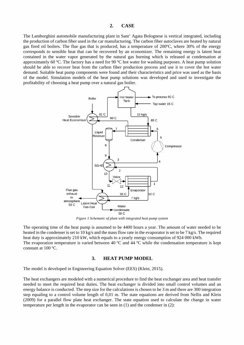
2. CASE

The Lamborghini automobile manufacturing plant in Sant’ Agata Bolognese is vertical integrated, including the production of carbon fiber used in the car manufacturing. The carbon fiber autoclaves are heated by natural gas fired oil boilers. The flue gas that is produced, has a temperature of 200ºC, where 30% of the energy corresponds to sensible heat that can be recovered by an economizer. The remaining energy is latent heat contained in the water vapor generated by the natural gas burning which is released at condensation at approximately 60 ºC. The factory has a need for 90 ºC hot water for washing purposes. A heat pump solution should be able to recover heat from the carbon fiber production process and use it to cover the hot water demand. Suitable heat pump components were found and their characteristics and price was used as the basis of the model. Simulation models of the heat pump solutions was developed and used to investigate the profitability of choosing a heat pump over a natural gas boiler.

Figure 1 Schematic of plant with integrated heat pump system

The operating time of the heat pump is assumed to be 4400 hours a year. The amount of water needed to be heated in the condenser is set to 10 kg/s and the mass flow rate in the evaporator is set to be 7 kg/s. The required heat duty is approximately 210 kW, which equals to a yearly energy consumption of 924 000 kWh. The evaporation temperature is varied between 40 ºC and 44 ºC while the condensation temperature is kept constant at 100 ºC.

3. HEAT PUMP MODEL

The model is developed in Engineering Equation Solver (EES) (Klein, 2015). The heat exchangers are modeled with a numerical procedure to find the heat exchanger area and heat transfer needed to meet the required heat duties. The heat exchanger is divided into small control volumes and an energy balance is conducted. The step size for the calculations is chosen to be 3 m and there are 300 integration step equaling to a control volume length of 0,01 m. The state equations are derived from Nellis and Klein (2009) for a parallel flow plate heat exchanger. The state equation used to calculate the change in water temperature per length in the evaporator can be seen in (1) and the condenser in (2):

𝑑𝑑𝑇𝑇𝐻𝐻𝑑𝑑𝑑𝑑

= − 2 𝑁𝑁𝑐𝑐ℎ(𝑇𝑇𝐻𝐻−𝑇𝑇𝐶𝐶)

�̇�𝑚ℎ𝑐𝑐𝐻𝐻�1

ℎ𝐻𝐻𝑊𝑊+ 𝑡𝑡ℎ𝑚𝑚𝑘𝑘𝑚𝑚𝑊𝑊+

1ℎ𝐶𝐶𝑊𝑊

� (1)

𝑑𝑑𝑇𝑇𝐶𝐶𝑑𝑑𝑑𝑑

= 2 𝑁𝑁𝑐𝑐ℎ(𝑇𝑇𝐻𝐻−𝑇𝑇𝐶𝐶)

�̇�𝑚𝐶𝐶𝑐𝑐𝐶𝐶�1

ℎ𝐻𝐻𝑤𝑤+𝑡𝑡ℎ𝑚𝑚𝑘𝑘𝑚𝑚𝑤𝑤+

1ℎ𝐶𝐶𝑤𝑤

� (2)

The change in temperature is used to calculate the enthalpy change, which in turn gives the heat transferred to or from the refrigerant. The next control volume is calculated on the basis of values of the previous control volume, this procedure will go on until the desired outlet conditions are met. The temperature change in the refrigerant is given by the saturation pressure. The saturation pressure is affected by a pressure drop in the heat exchanger leading to a temperature fall. The heat transfer coefficient is calculated using the Nusselt number:

ℎ = 𝑁𝑁𝑁𝑁 𝑘𝑘𝑑𝑑ℎ

(3)

The hydraulic diameter for both the evaporator and condenser is calculated using (Martin, 1996):

𝑑𝑑ℎ = 2𝑏𝑏Φ

(4)

Φ(𝑋𝑋) ≈ 16��1 + �(1 + 𝑋𝑋2) + 4�1 + 𝑋𝑋2

2�� (5)

𝑋𝑋 = 𝑏𝑏𝑏𝑏p

(6)

3.1. Evaporator The two-phase heat transfer coefficient is modeled with Amalfi et al. (2016b) correlation for flow boiling in plate heat exchangers in the region of 0<x<0,9:

𝑁𝑁𝑢𝑢𝑡𝑡𝑡𝑡 = �982 𝛽𝛽∗1,101 𝑊𝑊𝑊𝑊𝑚𝑚

0,315𝐵𝐵𝐵𝐵0,320𝜌𝜌∗−0,224 ,𝐵𝐵𝑑𝑑 < 418,495 𝛽𝛽∗0,248𝑅𝑅𝑊𝑊𝑣𝑣

0,135𝑅𝑅𝑊𝑊𝑙𝑙𝑙𝑙0,351𝐵𝐵𝑑𝑑0,235𝐵𝐵𝐵𝐵0,198𝜌𝜌∗−0,223,𝐵𝐵𝑑𝑑 ≥ 4

(7)

When the vapor quality is between 0,90<x<1 the heat transfer coefficient is modeled to decrease linearly down to 600 W/(m2K). When x=1 the heat transfer coefficient for the refrigerant is found using the Martin correlation for single-phase flow in a plate heat exchanger (García-Cascales et al., 2007):

𝑁𝑁𝑢𝑢 = 0,122𝑃𝑃𝑃𝑃13 � 𝜇𝜇

𝜇𝜇𝑤𝑤𝑤𝑤𝑤𝑤𝑤𝑤�16 (𝑓𝑓𝑅𝑅𝑊𝑊2 sin(2𝛽𝛽))0,374 (8)

The water side heat transfer coefficient is calculated using the Martin correlation for single-phase flow.

3.2. Condenser The heat transfer coefficient for the superheated and subcooled region are calculated using the Martin correlation for single-phase flow. The two-phase heat transfer coefficient is modeled with Longo et al. (2015) correlation for condensation in plate heat exchangers:

ℎ𝑠𝑠𝑠𝑠𝑡𝑡 = 1,875 Φ�𝑘𝑘𝑤𝑤𝑑𝑑ℎ� 𝑅𝑅𝑊𝑊𝑒𝑒𝑒𝑒

0,445𝑃𝑃𝑃𝑃𝑙𝑙1/3 (9)

Table 1 Inputs to Heat Exchangers

Inputs Value 𝐿𝐿 [m] 0,450 𝑊𝑊 [m] 0,243 𝑁𝑁𝑐𝑐ℎ [-] Variable

𝑝𝑝 [m] 0,008 𝑏𝑏 [m] 0,002 𝛽𝛽 [deg] 45 𝑇𝑇ℎ𝑚𝑚 [m] 0,0005

𝑇𝑇𝑠𝑠ℎ [K] 5

𝑇𝑇𝑠𝑠𝑐𝑐 [K] 1

3.3. Compressor The compressor work is calculated using isentropic efficiency and a heat loss. The heat loss is constant and equal to 10% of the compressor work. The isentropic and volumetric efficiency is calculated using the pressure ratio (Eikevik et al., 2016): 𝜂𝜂𝑖𝑖𝑠𝑠 = −0,00000461 𝑃𝑃𝑅𝑅6 + 0,00027131 𝑃𝑃𝑅𝑅5 − 0,00628605 𝑃𝑃𝑅𝑅4 + 0,07370258 𝑃𝑃𝑅𝑅3 −0,46054399 𝑃𝑃𝑅𝑅2 + 1,40653347 𝑃𝑃𝑅𝑅 − 0,87811477 (10)

λ = 0,0011 𝑃𝑃𝑅𝑅2 − 0,0487 𝑃𝑃𝑅𝑅 + 0,9979 (11)

3.4. Suction Gas Heat Exchanger The R600 and R600a models have an additional superheat of 10 K and a constant pressure drop around 50 kPa. R1234ze(Z) is modelled without a suction gas heat exchanger and therefore no additional pressure drop.

3.5. Pressure Loss in the System The total pressure loss in the heat exchangers is calculated using (Amalfi et al., 2016a) and (Longo, 2010):

Δ𝑃𝑃𝑡𝑡𝑙𝑙𝑡𝑡,𝑒𝑒𝑣𝑣𝑠𝑠𝑡𝑡 = Δ𝑃𝑃𝐺𝐺 + Δ𝑃𝑃𝑠𝑠𝑐𝑐𝑐𝑐 + Δ𝑃𝑃𝑓𝑓𝑟𝑟𝑖𝑖𝑐𝑐 + Δ𝑃𝑃𝑡𝑡 (12)

Δ𝑃𝑃𝑡𝑡𝑙𝑙𝑡𝑡,𝑐𝑐𝑙𝑙𝑐𝑐𝑑𝑑 = −Δ𝑃𝑃𝐺𝐺 − Δ𝑃𝑃𝑠𝑠𝑐𝑐𝑐𝑐 + Δ𝑃𝑃𝑓𝑓𝑟𝑟𝑖𝑖𝑐𝑐 + Δ𝑃𝑃𝑡𝑡 (13)

Δ𝑃𝑃𝐺𝐺 = 𝜌𝜌𝑚𝑚 𝑔𝑔 𝐿𝐿𝑡𝑡𝑙𝑙𝑠𝑠𝑡𝑡𝑒𝑒 (14)

Δ𝑃𝑃𝑠𝑠𝑐𝑐𝑐𝑐 = 𝐺𝐺2Δ𝑥𝑥 � 1𝜌𝜌𝑔𝑔− 1

𝜌𝜌𝑤𝑤� (15)

Δ𝑃𝑃𝑡𝑡 = 0,75 � �𝐺𝐺𝑝𝑝2

2𝜌𝜌�𝑖𝑖𝑐𝑐

+ �𝐺𝐺𝑝𝑝2

2𝜌𝜌�𝑙𝑙𝑁𝑁𝑡𝑡

� (16)

The frictional pressure drop in the evaporator caused by the refrigerant is predicted using two-phase friction factor coefficient from (Amalfi et al., 2016b) and the friction factor coefficient from Martin correlation for single phase flow (García-Cascales et al., 2007):

Δ𝑃𝑃𝑓𝑓𝑟𝑟𝑖𝑖𝑐𝑐 = 2 𝑓𝑓 𝐺𝐺2Δ𝑦𝑦𝑑𝑑ℎ∗𝜌𝜌𝑚𝑚

(17)

The frictional pressure drop in the condenser is predicted using a linear equation based on the kinetic energy per unit volume from (Longo, 2010) given in kPa:

Δ𝑃𝑃𝑓𝑓𝑟𝑟𝑖𝑖𝑐𝑐 = 1,90 𝐾𝐾𝐾𝐾𝑉𝑉

(18)

𝐾𝐾𝐾𝐾𝑉𝑉

= 𝐺𝐺2

2 𝜌𝜌𝑚𝑚 (19)

The pressure loss in the pipes are calculated using the function PipeFlow (Klein, 2015). The pipe diameter is chosen on the basis of having flow velocities of around 9-10 m/s in the suction line, 6-7 m/s in the pressure pipeline and 2-3,5 m/s in the return lines to have an efficient oil return and moderate pressure/temperature loss.

3.6. Iterative Optimization A set of error functions are used to find the correct input values that corresponds with the different operating conditions. EES’ inbuilt MIN/MAX function was used to find the correct mass flow of the refrigerant at the base operating conditions by minimizing:

errtemp;cond = abs(Tw;real;out − Twater;out;cond) (20)

The correct compressor outlet pressure was found minimizing the error function:

𝑊𝑊𝑃𝑃𝑃𝑃𝑐𝑐𝑙𝑙𝑚𝑚𝑡𝑡 = 𝑎𝑎𝑏𝑏𝑎𝑎(𝑃𝑃𝑔𝑔𝑁𝑁𝑒𝑒𝑠𝑠𝑠𝑠;𝑐𝑐𝑙𝑙𝑚𝑚𝑡𝑡 − Δ𝑃𝑃56) (21)

The number channels in the evaporator and condenser was found by minimizing:

𝑊𝑊𝑃𝑃𝑃𝑃𝑙𝑙𝑒𝑒𝑐𝑐𝑔𝑔𝑡𝑡ℎ;𝑐𝑐𝑙𝑙𝑐𝑐𝑑𝑑 = 𝑎𝑎𝑏𝑏𝑎𝑎(𝐿𝐿𝑡𝑡𝑙𝑙𝑠𝑠𝑡𝑡𝑒𝑒;𝑐𝑐𝑙𝑙𝑐𝑐𝑑𝑑 − 𝐿𝐿𝑙𝑙𝑁𝑁𝑡𝑡;𝑐𝑐𝑙𝑙𝑐𝑐𝑑𝑑) (22)

𝑊𝑊𝑃𝑃𝑃𝑃𝑙𝑙𝑒𝑒𝑐𝑐𝑔𝑔𝑡𝑡ℎ;𝑒𝑒𝑣𝑣𝑠𝑠𝑡𝑡 = 𝑎𝑎𝑏𝑏𝑎𝑎(𝐿𝐿𝑡𝑡𝑙𝑙𝑠𝑠𝑡𝑡𝑒𝑒;𝑒𝑒𝑣𝑣𝑠𝑠𝑡𝑡 − 𝐿𝐿𝑙𝑙𝑁𝑁𝑡𝑡;𝑒𝑒𝑣𝑣𝑠𝑠𝑡𝑡) (23)

3.7. Economic Model An economic model has been created to compare the operational and investment costs of the different heat pump solutions in addition to comparing them with a traditional heating solution. In this case a natural gas boiler is used for comparison. The annual cost for the different solutions is calculated by summing the annual capital cost, the annual operational cost and the annual maintenance cost. The maintenance cost is calculated as a percentage of the investment cost:

𝐴𝐴𝐴𝐴 = ∑(𝐼𝐼0 𝑎𝑎)𝑐𝑐 + ∑(𝑊𝑊𝑒𝑒 𝑊𝑊) + ∑𝑀𝑀𝐴𝐴 (24)

To assess if it is profitable to invest in the different heat pump solutions over a natural gas boiler a profitability analysis is conducted. This is done using the Present Value Method and Pay-Off Time (Stene, 2016). The Present Value Method shows the absolute profitability of an investment. If a heat pump project has a PV>0 then its regarded as a profitable investment. PV is calculated by:

𝑃𝑃𝑃𝑃 = 𝐵𝐵𝑠𝑠− 𝐼𝐼0 (25)

Pay-Off Time will result in the number of years it takes before the sum of net annual savings equals to the additional investment cost, while taking account of the real interest rate. Pay-Off Time is calculated by:

𝑃𝑃𝑃𝑃=𝑙𝑙𝑐𝑐��1−�𝐼𝐼0𝐵𝐵�𝑟𝑟�

−1�

𝑙𝑙𝑐𝑐(1+𝑟𝑟) (26)

Table 2 Inputs in economic model

Inputs Value

𝑃𝑃 [%] 5

𝑛𝑛 [years] 25

𝜏𝜏 [hours] 4400

𝑄𝑄 [kW] 210

𝐸𝐸𝑡𝑡𝑙𝑙𝑡𝑡 [kWh] 924 000

𝑀𝑀𝐴𝐴𝐻𝐻𝐻𝐻 [%] 6

𝑀𝑀𝐴𝐴𝑔𝑔𝑠𝑠𝑠𝑠 [%] 3

η𝑔𝑔𝑠𝑠𝑠𝑠 [-] 0,95

egas [NOK/kWh] 0,37

eel [NOK/kWh] 1,10

4. RESULTS

4.1. Heat Pump Model Table 3 shows the results of some of the most important variables for the 3 different refrigerants at changing evaporating temperatures.

Table 3 Simulation results for the different refrigerants at different evaporation temperatures

R600 𝑇𝑇𝑒𝑒𝑣𝑣𝑠𝑠𝑡𝑡 𝑊𝑊 𝑃𝑃𝑠𝑠 𝐴𝐴𝑃𝑃𝑃𝑃 𝑁𝑁𝑐𝑐ℎ;𝑒𝑒𝑣𝑣𝑠𝑠𝑡𝑡 𝑁𝑁𝑐𝑐ℎ;𝑐𝑐𝑙𝑙𝑐𝑐𝑑𝑑 𝑈𝑈𝑐𝑐𝑙𝑙𝑐𝑐𝑑𝑑 𝑈𝑈𝑒𝑒𝑣𝑣𝑠𝑠𝑡𝑡 Δ𝑃𝑃𝑒𝑒𝑣𝑣𝑠𝑠𝑡𝑡 Δ𝑃𝑃𝑐𝑐𝑙𝑙𝑐𝑐𝑑𝑑 𝑃𝑃𝑅𝑅 �̇�𝑚𝑟𝑟𝑒𝑒𝑓𝑓 40 ºC 75487 508,2 2,826 15 47 1108 4637 52684 2297 5,563 0,67 41 ºC 69037 456,9 3,029 18 44 1232 4544 39398 2742 5,116 0,67 42 ºC 64226 419,2 3,196 22 41 1330 4476 29025 3298 4,775 0,67 43 ºC 60564 390,6 3,35 27 39 1434 4381 21558 3738 4,512 0,67 44 ºC 57553 366,7 3,484 35 38 1466 4598 15028 3981 4,285 0,67 R600a 𝑇𝑇𝑒𝑒𝑣𝑣𝑠𝑠𝑡𝑡 𝑊𝑊 𝑃𝑃𝑠𝑠 𝐴𝐴𝑃𝑃𝑃𝑃 𝑁𝑁𝑐𝑐ℎ;𝑒𝑒𝑣𝑣𝑠𝑠𝑡𝑡 𝑁𝑁𝑐𝑐ℎ;𝑐𝑐𝑙𝑙𝑐𝑐𝑑𝑑 𝑈𝑈𝑐𝑐𝑙𝑙𝑐𝑐𝑑𝑑 𝑈𝑈𝑒𝑒𝑣𝑣𝑠𝑠𝑡𝑡 Δ𝑃𝑃𝑒𝑒𝑣𝑣𝑠𝑠𝑡𝑡 Δ𝑃𝑃𝑐𝑐𝑙𝑙𝑐𝑐𝑑𝑑 𝑃𝑃𝑅𝑅 �̇�𝑚𝑟𝑟𝑒𝑒𝑓𝑓 40 ºC 73760 376,8 2,835 14 45 1218 4724 63781 4358 4,789 0,8 41 ºC 69122 348,7 2,966 16 42 1308 4629 51757 5128 4,505 0,8 42 ºC 64878 322,4 3,123 20 40 1386 4510 37039 5741 4,226 0,8 43 ºC 61733 302,8 3,27 25 40 1429 4423 26936 5728 4,015 0,8 44 ºC 59398 287,4 3,399 33 40 1426 5711 18782 5729 3,836 0,8 R1234ze(Z) 𝑇𝑇𝑒𝑒𝑣𝑣𝑠𝑠𝑡𝑡 𝑊𝑊 𝑃𝑃𝑠𝑠 𝐴𝐴𝑃𝑃𝑃𝑃 𝑁𝑁𝑐𝑐ℎ;𝑒𝑒𝑣𝑣𝑠𝑠𝑡𝑡 𝑁𝑁𝑐𝑐ℎ;𝑐𝑐𝑙𝑙𝑐𝑐𝑑𝑑 𝑈𝑈𝑐𝑐𝑙𝑙𝑐𝑐𝑑𝑑 𝑈𝑈𝑒𝑒𝑣𝑣𝑠𝑠𝑡𝑡 Δ𝑃𝑃𝑒𝑒𝑣𝑣𝑠𝑠𝑡𝑡 Δ𝑃𝑃𝑐𝑐𝑙𝑙𝑐𝑐𝑑𝑑 𝑃𝑃𝑅𝑅 �̇�𝑚𝑟𝑟𝑒𝑒𝑓𝑓 40 ºC 71580 543 2,961 17 60 772,8 3756 65761 1064 6,026 1,18 41 ºC 64057 475,5 3,216 20 54 900,8 3730 50659 1728 5,439 1,18 42 ºC 58515 427,5 3,424 24 51 953,7 3633 38448 2136 5,006 1,18 43 ºC 54608 393,9 3,629 29 49 1042 3583 29960 2453 4,688 1,18 44 ºC 51300 365,2 3,824 37 47 1121 3715 21212 2822 4,41 1,18

4.2. Economic Model Figure 2 shows the annual cost for the 3 heat pumps and Figure 3 and Figure 4 shows the corresponding present value and pay-off time. In Figure 5 to Figure 7 is the results of a sensitivity analysis for the R1234ze(Z) heat pump at varying electricity prices. In Figure 8 to Figure 10 is the results of a sensitivity analysis for R1234ze(Z) heat pump at varying natural gas prices. R1234ze(Z) was used, because it was the most cost efficient cycle of the three.

Figure 2 Annual Cost for different evaporation temperatures

Figure 3 Present value for different evaporation temperatures

300000325000350000375000400000425000450000

40 41 42 43 44Ann

ual C

ost [

NO

K/y

ear]


R600 R600a

R1234ze(Z) Gas Boiler

0100000200000300000400000500000600000700000800000900000

40 41 42 43 44

Pres

ent V

alue

[NO

K]


R600 R600a R1234ze(Z)

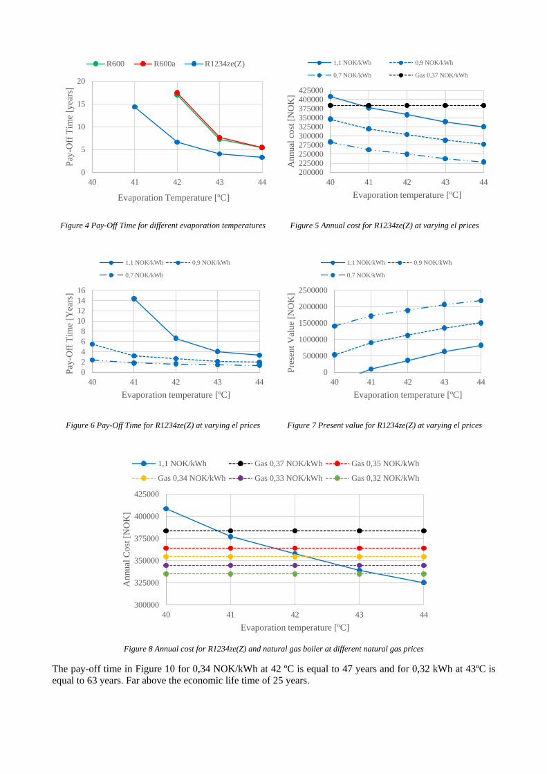
Figure 4 Pay-Off Time for different evaporation temperatures

Figure 5 Annual cost for R1234ze(Z) at varying el prices

Figure 6 Pay-Off Time for R1234ze(Z) at varying el prices

Figure 7 Present value for R1234ze(Z) at varying el prices

Figure 8 Annual cost for R1234ze(Z) and natural gas boiler at different natural gas prices

The pay-off time in Figure 10 for 0,34 NOK/kWh at 42 ºC is equal to 47 years and for 0,32 kWh at 43ºC is equal to 63 years. Far above the economic life time of 25 years.

0

5

10

15

20

40 41 42 43 44

Pay-

Off

Tim

e [y

ears

]


R600 R600a R1234ze(Z)

200000225000250000275000300000325000350000375000400000425000

40 41 42 43 44

Ann

ual c

ost [

NO

K]


1,1 NOK/kWh 0,9 NOK/kWh

0,7 NOK/kWh Gas 0,37 NOK/kWh

02468

10121416

40 41 42 43 44

Pay-

Off

Tim

e [Y

ears

]



0,7 NOK/kWh

0

500000

1000000

1500000

2000000

2500000

40 41 42 43 44

Pres

ent V

alue

[NO

K]



0,7 NOK/kWh

300000

325000

350000

375000

400000

425000

40 41 42 43 44

Ann

ual C

ost [

NO

K]


1,1 NOK/kWh Gas 0,37 NOK/kWh Gas 0,35 NOK/kWh


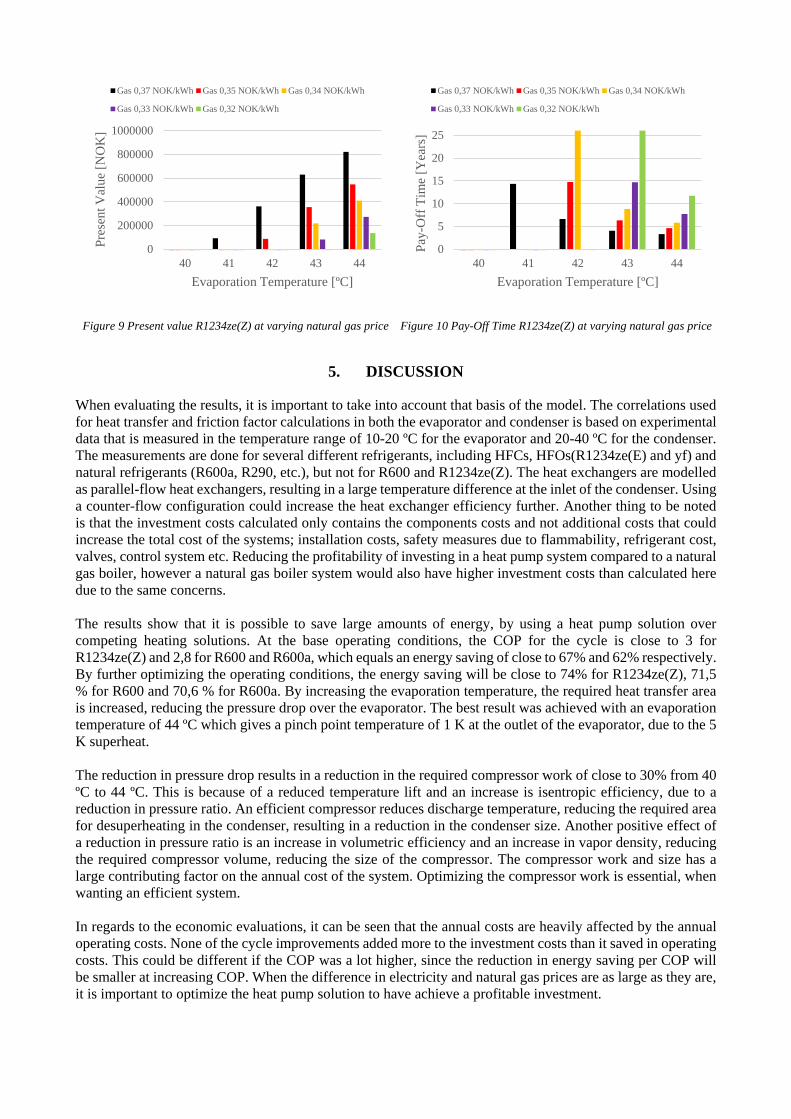
Figure 9 Present value R1234ze(Z) at varying natural gas price

Figure 10 Pay-Off Time R1234ze(Z) at varying natural gas price

5. DISCUSSION

When evaluating the results, it is important to take into account that basis of the model. The correlations used for heat transfer and friction factor calculations in both the evaporator and condenser is based on experimental data that is measured in the temperature range of 10-20 ºC for the evaporator and 20-40 ºC for the condenser. The measurements are done for several different refrigerants, including HFCs, HFOs(R1234ze(E) and yf) and natural refrigerants (R600a, R290, etc.), but not for R600 and R1234ze(Z). The heat exchangers are modelled as parallel-flow heat exchangers, resulting in a large temperature difference at the inlet of the condenser. Using a counter-flow configuration could increase the heat exchanger efficiency further. Another thing to be noted is that the investment costs calculated only contains the components costs and not additional costs that could increase the total cost of the systems; installation costs, safety measures due to flammability, refrigerant cost, valves, control system etc. Reducing the profitability of investing in a heat pump system compared to a natural gas boiler, however a natural gas boiler system would also have higher investment costs than calculated here due to the same concerns. The results show that it is possible to save large amounts of energy, by using a heat pump solution over competing heating solutions. At the base operating conditions, the COP for the cycle is close to 3 for R1234ze(Z) and 2,8 for R600 and R600a, which equals an energy saving of close to 67% and 62% respectively. By further optimizing the operating conditions, the energy saving will be close to 74% for R1234ze(Z), 71,5 % for R600 and 70,6 % for R600a. By increasing the evaporation temperature, the required heat transfer area is increased, reducing the pressure drop over the evaporator. The best result was achieved with an evaporation temperature of 44 ºC which gives a pinch point temperature of 1 K at the outlet of the evaporator, due to the 5 K superheat. The reduction in pressure drop results in a reduction in the required compressor work of close to 30% from 40 ºC to 44 ºC. This is because of a reduced temperature lift and an increase is isentropic efficiency, due to a reduction in pressure ratio. An efficient compressor reduces discharge temperature, reducing the required area for desuperheating in the condenser, resulting in a reduction in the condenser size. Another positive effect of a reduction in pressure ratio is an increase in volumetric efficiency and an increase in vapor density, reducing the required compressor volume, reducing the size of the compressor. The compressor work and size has a large contributing factor on the annual cost of the system. Optimizing the compressor work is essential, when wanting an efficient system. In regards to the economic evaluations, it can be seen that the annual costs are heavily affected by the annual operating costs. None of the cycle improvements added more to the investment costs than it saved in operating costs. This could be different if the COP was a lot higher, since the reduction in energy saving per COP will be smaller at increasing COP. When the difference in electricity and natural gas prices are as large as they are, it is important to optimize the heat pump solution to have achieve a profitable investment.

0

200000

400000

600000

800000

1000000

40 41 42 43 44

Pres

ent V

alue

[NO

K]




0

5

10

15

20

25

40 41 42 43 44

Pay-

Off

Tim

e [Y

ears

]




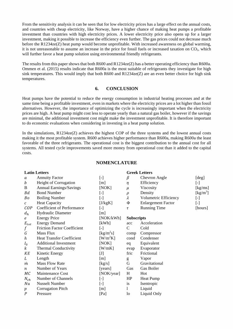
From the sensitivity analysis it can be seen that for low electricity prices has a large effect on the annual costs, and countries with cheap electricity, like Norway, have a higher chance of making heat pumps a profitable investment than countries with high electricity prices. A lower electricity price also opens up for a larger investment, making it possible to increase the efficiency even further. The gas prices could not decrease much before the R1234ze(Z) heat pump would become unprofitable. With increased awareness on global warming, it is not unreasonable to assume an increase in the price for fossil fuels or increased taxation on CO2, which will further favor a heat pump solution using environmental friendly refrigerants. The results from this paper shows that both R600 and R1234ze(Z) has a better operating efficiency than R600a. Ommen et al. (2015) results indicate that R600a is the most suitable of refrigerants they investigate for high sink temperatures. This would imply that both R600 and R1234ze(Z) are an even better choice for high sink temperatures.

6. CONCLUSION

Heat pumps have the potential to reduce the energy consumption in industrial heating processes and at the same time being a profitable investment, even in markets where the electricity prices are a lot higher than fossil alternatives. However, the importance of optimizing the cycle is increasingly important when the electricity prices are high. A heat pump might cost less to operate yearly than a natural gas boiler, however if the savings are minimal, the additional investment cost might make the investment unprofitable. It is therefore important to do economic evaluations when considering in investing in a heat pump solution. In the simulations, R1234ze(Z) achieves the highest COP of the three systems and the lowest annual costs making it the most profitable system. R600 achieves higher performance than R600a, making R600a the least favorable of the three refrigerants. The operational cost is the biggest contribution to the annual cost for all systems. All tested cycle improvements saved more money from operational cost than it added to the capital costs.

NOMENCLATURE

Latin Letters Greek Letters 𝑎𝑎 Annuity Factor [-] 𝛽𝛽 Chevron Angle [deg] 𝑏𝑏 Height of Corrugation [m] 𝜂𝜂 Efficiency [-] B Annual Earnings/Savings [NOK] 𝜇𝜇 Viscosity [kg/ms] 𝐵𝐵𝑑𝑑 Bond Number [-] 𝜌𝜌 Density [kg/m3] 𝐵𝐵𝐵𝐵 Boiling Number [-] 𝜆𝜆 Volumetric Efficiency [-] 𝑐𝑐 Heat Capacity [J/kgK] Φ Enlargement Factor [-] 𝐴𝐴𝑃𝑃𝑃𝑃 Coefficient of Performance [-] 𝜏𝜏 Running Time [hours] 𝑑𝑑ℎ Hydraulic Diameter [m] 𝑊𝑊 Energy Price [NOK/kWh] Subscripts 𝐸𝐸𝑡𝑡𝑙𝑙𝑡𝑡 Energy Demand [kWh] acc Acceleration 𝑓𝑓 Friction Factor Coefficient [-] C Cold 𝐺𝐺 Mass Flux [kg/m2s] comp Compressor ℎ Heat Transfer Coefficient [W/m2K] cond Condenser 𝐼𝐼0 Additional Investment [NOK] eq Equivalent 𝑘𝑘 Thermal Conductivity [W/mK] evap Evaporator 𝐾𝐾𝐸𝐸 Kinetic Energy [J] fric Frictional 𝐿𝐿 Length [m] g Vapor �̇�𝑚 Mass Flow Rate [kg/s] G Gravitational 𝑛𝑛 Number of Years [years] Gas Gas Boiler 𝑀𝑀𝐴𝐴 Maintenance Cost [NOK/year] H Hot 𝑁𝑁𝑐𝑐ℎ Number of Channels [-] HP Heat Pump 𝑁𝑁𝑢𝑢 Nusselt Number [-] is Isentropic 𝑝𝑝 Corrugation Pitch [m] l Liquid 𝑃𝑃 Pressure [Pa] lo Liquid Only

𝑄𝑄 Heat Duty [W] m Mean/Homogenous 𝑃𝑃𝑃𝑃 Prandtl Number [-] p Port 𝑃𝑃𝑅𝑅 Pressure Ratio [-] plate Heat Exchanger Plate 𝑃𝑃 Real Interest Rate [%] sc Subcool 𝑅𝑅𝑊𝑊 Reynolds Number [-] sh Superheat 𝑇𝑇 Temperature [K] tot Total 𝑡𝑡ℎ𝑚𝑚 Thickness of Plate [m] tp Two-Phase 𝑈𝑈 Overall Heat Transfer Coefficient [W/m2K] wall Plate wall 𝑃𝑃 Volume [m3] 𝑃𝑃𝑠𝑠 Required Compressor Volume [m3/h] 𝑊𝑊 Work [W] 𝑤𝑤 Width [m] 𝑊𝑊𝑊𝑊 Weber Number [-] 𝑦𝑦 Length [m]

REFERENCES

AMALFI, R. L., VAKILI-FARAHANI, F. & THOME, J. R. 2016a. Flow boiling and frictional pressure gradients in plate heat exchangers. Part 1: Review and experimental database. International Journal of Refrigeration, 61, 166-184.

AMALFI, R. L., VAKILI-FARAHANI, F. & THOME, J. R. 2016b. Flow boiling and frictional pressure gradients in plate heat exchangers. Part 2: Comparison of literature methods to database and new prediction methods. International Journal of Refrigeration, 61, 185-203.

CALM, J. M. 2008. The next generation of refrigerants – Historical review, considerations, and outlook. International Journal of Refrigeration, 31, 1123-1133.

CHUA, K. J., CHOU, S. K. & YANG, W. M. 2010. Advances in heat pump systems: A review. Applied Energy, 87, 3611-3624.

EIKEVIK, T. M., TOLSTOREBROV, I., BREDESEN, A. M., REKSTAD, H., PETTERSEN, J., AFLEKT, K. & ELGSÆTHER, M. 2016. TEP 4255 - Heat pumping processes and systems, NTNU, NTNU EPT.

FUKUDA, S., KONDOU, C., TAKATA, N. & KOYAMA, S. 2014. Low GWP refrigerants R1234ze(E) and R1234ze(Z) for high temperature heat pumps. International Journal of Refrigeration, 40, 161-173.

GARCÍA-CASCALES, J. R., VERA-GARCÍA, F., CORBERÁN-SALVADOR, J. M. & GONZÁLVEZ-MACIÁ, J. 2007. Assessment of boiling and condensation heat transfer correlations in the modelling of plate heat exchangers. International Journal of Refrigeration, 30, 1029-1041.

IEA-HPC 2014. Application of Industrial Heat Pumps, Part 2. IEA HPP ANNEX 35. International Energy Agency Heat Pump Centre.

KLEIN, S. 2015. Engineering Equation Solver Professional 9.935-3D. Madison, WI: F-Chart Software. KONDOU, C. & KOYAMA, S. 2015. Thermodynamic assessment of high-temperature heat pumps using

Low-GWP HFO refrigerants for heat recovery. International Journal of Refrigeration, 53, 126-141. LONGO, G. A. 2010. Heat transfer and pressure drop during hydrocarbon refrigerant condensation inside a

brazed plate heat exchanger. International Journal of Refrigeration, 33, 944-953. LONGO, G. A., RIGHETTI, G. & ZILIO, C. 2015. A new computational procedure for refrigerant

condensation inside herringbone-type Brazed Plate Heat Exchangers. International Journal of Heat and Mass Transfer, 82, 530-536.

MARTIN, H. 1996. A theoretical approach to predict the performance of chevron-type plate heat exchangers. Chemical Engineering and Processing: Process Intensification, 35, 301-310.

NELLIS, G. & KLEIN, S. 2009. Heat transfer, Cambridge, Cambridge University Press. OMMEN, T., JENSEN, J. K., MARKUSSEN, W. B., REINHOLDT, L. & ELMEGAARD, B. 2015. Technical

and economic working domains of industrial heat pumps: Part 1 – Single stage vapour compression heat pumps. International Journal of Refrigeration, 55, 168-182.

Cost Efficient Industrial Heat Recovery through Heat Pumps

Documents

Transcript of Cost Efficient Industrial Heat Recovery through Heat Pumps