Cost‐effective Methods for Monitoring Coarse Woody Debris in 

Northeastern Forests 

 

By John Williamson 

May  2008 

 

Dr. Daniel deB. Richter, Adviser

Masters project proposal submitted in partial fulfillment of the requirements for the

Master of Environmental Management and Master of Forestry degrees in the

Nicholas School of the Environment and Earth Sciences of Duke University.

Abstract. Across boreal and temperate biomes, the area of old forests is in global decline, with the consequent extinction of dependent species posing a major threat to biodiversity. As such, current sustainable forestry certification programs position management for biodiversity as a fundamental goal. Yet, to do so necessitates both the use of effective indicators, of which downed coarse woody debris (CWD) is well-established, and the establishment of reference levels, which are most often based on comparable old growth systems. However, the extreme spatial variability of CWD makes inventorying and monitoring this structural attribute problematic. Trade-offs exist between costs, sampling methods, sample area, and the statistical ability to detect change. Faced with vast uncertainty regarding the effectiveness of monitoring approaches, large-scale inventories of CWD are largely neglected in the Northeast. The objectives of this project were two-fold: 1) to develop cost-effective methods for monitoring coarse woody debris volume at a scale appropriate to northeastern forest management and 2) to discern the potential impacts of forest management on CWD attributes. A systematic sampling approach was used to inventory CWD in a managed and an old growth forest in Northern Maine. Two promising methods for measuring CWD—line intersect sampling and perpendicular distance sampling—were compared in the managed landscape, using different sampling areas for each approach. Perpendicular distance sampling exhibited high sampling costs and poor statistical efficiency relative to line intersect sampling. As such, it cannot be recommended for large-scale forest inventories. Only line intersect sampling was used in the old growth forest. Doing so enabled comparison of the statistical efficiencies of varying transect length and CWD attributes between landscapes. Power analyses were conducted to determine the tradeoffs between statistical precision and sample effort in using a particular transect length for inventorying CWD in managed and unmanaged forests. Variance was reduced with increasing transect length. However, choosing the appropriate transect length for a large-scale inventory depends on the level of precision required and the sensitivity to change in CWD volume for a given landscape. Land managers can consult these graphs to determine the appropriate minimum sample size required on average to detect a specific change in CWD volume at an accepted power and alpha level. Further, the old growth forest had more than twice the mean CWD volume than in the managed landscape, and landscapes differed in how this volume was distributed across size and decay classes, suggesting insight into the impacts of forest management on CWD.

2

Table of Contents 1. Introduction……………………………………………………………………………p. 4 – 8 2. Methods………………………………………………………………………………. p. 8-18 3. Results……………………………………………………………………………….....p.19-23. 4. Discussion……………………………………………………………………………...p. 24-35 5. Literature Cited……………………………………………………………………….p. 36-41 6. Appendix………………………………………………………………………………p. 41-52

3

1. Introduction:

Across boreal and temperate biomes, retention of old growth forests is paramount for

biodiversity conservation given the pandemic loss of such forests and the subsequent threat to

dependent species (Freedman et al. 1996, Noss 1999, Hanski 2000, Berg et al. 1994). In many

countries, such as Sweden, with an extensive history of forest management, intensive practices

have spurred this decline by reducing the structural diversity of forest systems —the effects of

which have only recently been recognized. In response, the forest management paradigm has

shifted focus from fiber production towards a more holistic ecosystem-based approach (Hansen

et al. 1991, Swanson and Franklin 1992), evidenced in the fact that many forestry certification

programs include biodiversity as a fundamental goal. However, biodiversity is an overly

complex entity to manage for, necessitating the use of efficient and effective indicators (Noss

1999, Lindenmayer et al. 2000, Hagan and Whitman 2006).

Old growth forests are characterized by unique structural features that develop over long

time scales and as such, are largely absent from younger stands. Among these, perhaps the most

important, recognized as indicators for forest health, are the density of large trees and snags and

downed coarse woody debris (CWD) attributes. The structural heterogeneity provided by large

trees, large snags, and downed woody debris both affects resource availability for an abundance

of species across taxa and alters abiotic conditions, leading to increased forest biodiversity

(Maser et al. 1979, Harmon et al. 1986).

Both when alive and dead, large trees serve as critical substrate for many forest species

currently recognized as rare or threatened, including several epiphytic bryophytes and lichens

(Lesica et al. 1991, Rose 1992, Selva 1994, Samuelsson et al. 1994, Esseen et al. 1996). Large

trees further provide shelter for wildlife (e.g. dens for furbearers); cavities for large-bodied birds,

4

such as woodpeckers, and later secondary cavity species (DeGraff and Rudis 1986, Tubbs et al.

1987, Hagan and Grove 1999); perching, nesting, foraging, and roosting sites for a variety of

other bird species (DeGraff and Rudis 1982, Tubbs et al. 1987); and specialized habitat for

arthropods (Harmon et al. 1986, Warren and Key 1991). Once dead, large trees serve as food

and foraging substrate for many vertebrate and invertebrate species (Harmon et al. 1986,

Samuelsson 1994, Hagan and Grove 1999). More over, the residence time of a dead tree may

extend centuries, prolonging its ecological importance (Franklin et al. 1987). Both brought about

by and exerting positive feedback on forest disturbance processes (Tinker and Knight 2001,

Turner et al. 2003), large and downed coarse woody debris (CWD) is ecologically important in

terrestrial and aquatic systems (Harmon et al. 1986). Ecosystem processes influenced by CWD

include nutrient cycling through the storage and slow release of nutrients (Harmon et al. 1986,

Harmon and Hua 1991, Jurgensen et al. 1997); soil development (Harvey and Neuenschwander

1991) and forest floor microtopography by providing organic material, altering runoff, reducing

soil erosion and constructing pit-and-mound formations; and fire intensity and return interval

(Beatty and Stone 1986, Harmon et al. 1986). CWD is a critical store for carbon (Harmon and

Hua 1991, Turner et. al 1994) and moisture in forested systems (Harmon et al. 1986, Fraver

2002). Downed woody debris serves as important growing substrate for fungi, lichen, moss, and

liverwort species (Berg et al. 1994), habitat for forest vertebrate and invertebrate species

(Harmon et al. 1986, Niemela 1997), and a seedbed for many vascular plant species (Maser et al.

1979, Marie-Josee et al. 1998).

Given the value of large trees, snags, and CWD as indicators of forest health and

recognizing their role in ecosystem processes, most contemporary forest policies mandate

management for these attributes. For example, Criterion no. 5, as devised in the 1994 Montréal

5

process and specified in the 1995 Santiago Declaration, requires maintenance of forest

contribution to the global carbon cycle through quantifying carbon fluxes in standing, dead, and

downed plant biomass, as well as soil. Thus, measurement of these attributes have become more

frequently incorporated into monitoring programs at various scales, ranging from national and

regional inventories to those on forest industry lands (Ståhl et al. 2001). In Maine, the two

predominant forestry certification programs require the management of structural attributes and

the assessment of forest habitat types. Specifically, the Sustainable Forestry Initiative (SFI)

requires landowners to “have programs to promote biological diversity at stand and landscape

levels” (1) to manage for important “stand-level wildlife habitat elements . . . [such as] snags . . .

[and] down woody debris” (Indicator 4.1.4), (2) to conduct assessments of “forest cover types

and habitats” (Indicator 4.1.5), and (3) to support the “conservation of old-growth forests in the

region” (Indicator 4.1.6) (AFPA 2004). Likewise, compliance with the Northeastern Forest

Stewardship Council (FSC) standard mandates landowners (1) “maintain . . . large fallen trees,

large logs, and snags of various sizes” (Indicator 6.3.b3) and (2) manage for “a distribution of

age classes appropriate to the size of ownership” (Indicator 6.3.a4) (Northeast Region Working

Group 2005).

Yet, the objectives are vaguely stated and lack clear direction regarding the best

approaches for inventorying and monitoring changes in these structural attributes. Regarding

CWD, a consistent definition is lacking (Helms 1998), and as such, existing studies often differ

in the dimensional and positional constraints of CWD based on project or management

objectives. Researchers and managers furthermore conduct measurements at different locations

along CWD pieces and differ in how these measurements are converted to volume estimates,

based on assumptions and taper equations (Stahl et al. 2001). Meta-analysis and other

6

comparisons among studies are therefore difficult. Adding to the management dilemma, CWD

parameters are challenging to inventory with great precision due to extreme variance in the

distribution and abundance of CWD within and between stands and across landscapes (Ståhl et

al. 2001). Equally prohibitive to monitoring CWD is the lack of financial return provided in

contrast to relatively high costs of estimation. Therefore, for a given inventory, methods should

be chosen so as to be (1) cost-efficient, (2) robust with regards to measurement error, (3) easy to

understand and simple to conduct, and (4) capable of providing additional contextual information

(Ståhl et al. 2001).

Various studies have examined the efficiency of current sampling techniques for CWD

(e.g., Ståhl et al. 2001, Bebber and Thomas 2001, Williams and Gove 2003); however they have

been insufficient in addressing the needs of northeastern forest managers: they are largely based

on computer simulations, limited in scope and scale, and applied in different geographic regions.

Further, none have examined the tradeoffs for methods between cost, effort (sample area and

sample size), and the statistical ability to detect change in CWD volume at the management scale

typical in the Northeast. Given these uncertainties, large-scale inventories of CWD are largely

neglected in the region. Yet, the ecological role of downed CWD in supporting forest

biodiversity is not withstanding: over 30% of mammals, 45% of amphibians, and 50% of reptiles

in New England utilize downed logs as foraging habitat or cover (DeGraff and Rudis 1986).

The objectives of our project are two fold. First, we sought to develop cost-effective

methods for monitoring CWD volume in northeastern forests by comparing the two most

promising inventory techniques for CWD across a range of management types. By presenting

the trade-offs between sampling effort—and thus cost—and the ability of land managers to

detect actual changes in CWD volume based on empirical, regionally-specific data, we hope to

7

direct the planning of future monitoring programs. Reference standards and management goals

for CWD volume and other attributes are most often based on old-growth conditions (Spies and

Franklin 1991, Keddy and Drummond 1996); however, estimation of these properties varies

greatly with the inventory methods used and the spatial scale of study (Shifley et al. 1994).

Therefore, our second objective was to discern the potential effects of forest management on

CWD through using similar methods to inventorying an intermediately managed and an old

growth forest in Northern Maine.

2. Methods:

2.1. Study areas

With ninety-percent of the land-cover (17.8 million acres) in forests, Maine remains the

most heavily forested state in the country (McWilliams et al. 2003). Unique to the state, forest

ownership in northern Maine is dominated by the commercial sector, with tracts typically

exceeding 50,000 hectares, much of which is certified under FSC or SFI (McWilliams et al.

2003). Regional cover types consist primarily of northern hardwood (NH) and upland spruce-fir

(SF) forests (40% and 33%, respectively), which is consistent throughout the Acadian Forest—a

region spanning northern New England and the Canadian Maritimes (McWilliams et al. 2003).

Dominant NH canopy species for sampled sites were Acer saccharum L. and Betula

alleghaniensis Britt. with Picea rubens Sarg., Betula papyrifera Marsh. var. cordifolia (Regel)

Fernald, Abies balsamea (L.) P. Mill as co-dominants. NH stands were typically located on

moderately drained loams and silt loams on mesic slopes and hilltops ranging from 150 to 700

meters in elevation (Whitman and Hagan 2003). SF stand were dominated by A. balsamea and

P. rubens with A. saccharum and Betula spp. frequent co-dominants. These stands occurred at

8

elevations between 150 and 1000 meters on moderately well-drained loams to mesic, clay loams

on hilltops, rocky slopes, and lower slopes (Whitman and Hagan 2003).

To meet the project objectives, the study was conducted in two landscapes: (1) an

intermediately managed, FSC-certified, commercial timberland spanning ~27,500-acres and

typical of forests in the region and (2) a ~5,400-acre old growth forest (Big Reed Reserve)

representative of the successional trajectory of Acadian forests with minimal anthropogenic

impact. Inventory of the managed landscape enabled development of sampling

recommendations for similar intermediately managed forests; whereas, the old growth forest

provided an approximation of appropriate sampling methods in unmanaged landscapes.

Modification of the sampling protocol for the old growth forest provided an adequate sampling

intensity to compare CWD attributes between the two landscapes.

Natural disturbance processes in these forests consist of frequent, small-scale gap formation

events from windthrow and snow. Large-scale, stand replacing disturbances are infrequent, with

the return interval at least an order of magnitude longer than gap-processes (Seymour et al. 2002,

Lorimer and White 2003). Infrequent spruce-budworm outbreaks have also had an impact with a

return interval several decades in length and the last outbreak from 1975-1985. The harvest

history of the managed landscape reflects that of northern Maine at large. Northern hardwood

forests have been high-graded for spruce since the 1800’s; for high-quality hardwoods beginning

in the 1900’s; and managed with selection harvesting since the 1960’s, transitioning to

shelterwood systems in the 1980’s (Whitman and Hagan 2007). Spruce-fir stands in the

managed landscape have been high-graded for conifers since the 1800’s. Heavy partial

harvesting and commercial clearcutting of SF stands began in the 1900s, with a transition to

silvicultural clearcutting or shelterwood systems continuing since in the 1960’s (Whitman and

9

Hagan, 2007). Though affected by natural disturbance processes, Big Reed Reserve exhibits

minimal impacts from timber harvesting according to both historical records and field

observations (Chokkalingam and White 2000).

2.2. Approach

Within the two landscapes, a systematic sampling approach using a random start was

chosen to replicate the standard approach for large-scale forest inventories; to ensure adequate

spatial coverage; and to minimize field crew travel costs (Marshall et al. 2000). For each

landscape, a kilometer-squared grid was overlain on a Universal Transverse Mercator projected

map using Arc GIS 9.x from which sampling blocks were randomly selected. Sample points

were then positioned at 200-meter intervals northward from the southwest to the northwest

corners of a block, with another line of sample points positioned 500-meters to the east. Where

inventory approaches would have intersected stand boundaries, sample points were randomly

shifted to the east or west to preclude boundary effects. Sites delineated as inoperable from

stand maps and ground-truthing in the managed landscape were randomly relocated at 200-meter

spacing north or south of the respective line of samples. A total of 108 sample points were

established in the managed landscape and 50 in the old growth stand. All sample points were

located in the field using a handheld GPS unit and compass.

Sampling approaches differed between the two landscapes to meet project objectives. In

the managed landscape, two methods for estimating CWD volume were performed at each

sample point to allow direct comparison between methods. Only one of these methods (LIS with

50-meter transects) was then used in the old growth. Inequality of sample size and sample area

(transect length) between landscapes was designed to capture the greater anticipated spatial

10

variance in CWD volume for the managed landscape and to enhance inventory

recommendations.

2.2.1. CWD Field Methods

Coarse woody debris was defined as dead tree boles, large limbs, and other large wood

pieces either lying on the ground or elevated less than 45° from horizontal and not self-

supporting having an average diameter > 7.5 cm at the point of measurement. Live material,

standing dead trees, stumps, dead foliage, and separated bark were not included. Constraints

were chosen to correspond with large-scale inventory approaches, such as the Forest Inventory

Analysis of the U.S. Forest Service and the Vegetation Resources Inventory in British Columbia,

Canada. The size-constraint further approximates the minimum diameter of 1000-hour fuels

used by the US Forest Service (Rothermel 1972). Length restrictions were not imposed.

Based on primary literature, the two methods chosen for estimating CWD volume were

line intersect sampling (LIS) and perpendicular distance sampling (PDS), due to their high

suitability for large-scale inventories. First applied to logging residue by Warren and Olson

(1964), LIS is one of the oldest and the most commonly used techniques for measuring CWD.

Preeminence and longevity have made LIS the most well-developed and adaptable method,

requiring minimal training time while providing high statistical efficiency in relation to sampling

cost (e.g., Canfield 1941, Warren and Olsen 1964, Van Wagner 1968, De Vries 1973, Kaiser

1983).

In the managed landscape, a 100-meter transect was established with fixed orientation

(east-west) and centered on the sample point. CWD pieces were then sampled if the central,

long-axis of the log was intersected. For curved logs or branched pieces with multiple

11

intersections, each intersection was measured independently when all other constraints were met.

At the point of intersection, two diameter measurements to the nearest centimeter were taken

perpendicular to the long axis of the log with metal calipers. Diameter was measured at the point

of intersection because of the unbiased nature of the measurement and the time efficiencies

gained by not leaving the transect (Van Wagner and Wilson 1976). Additional parameters

recorded for each piece included the species, decay class, and location along the transect (to

nearest 10 meter interval). Although decay is heterogeneous across individual logs (Pyle and

Brown 1999), overall decay stage can be accurately and rapidly estimated based on general

structural features (Pyle and Brown 1998). Using this approach, the decay stage of each log was

also recorded (Table 2).

Several novel sampling approaches have been developed for CWD in recent years,

including Diameter Relascope Samping (DRS) (Bebber and Thomas 2003), Transect Relascope

Sampling (TRS) (Ståhl 1998), Point Relascope Sampling (PRS) (Gove et al. 1999), and

Perpendicular Distance Sampling (PDS) (Williams and Gove 2003). Of these, simulation studies

suggest that PDS is the most statistically efficient for measuring CWD volume because the

inclusion probability is proportionate to piece volume rather than length, as with LIS and most

other methods. Sampling effort and bias are minimized, as well, because only borderline logs

must be measured (Williams and Gove 2003). Yet, few field studies have examined the

applicability of the method in the field, with the only published studies using simulation

approaches (Williams and Gove 2003, Williams et al. 2005). Using this method in the managed

landscape, logs were included if 1) a perpendicular angle (90°) could be constructed between the

long axis of the log and the sample point and 2) the distance of the log from the sample point was

less than the limiting distance relative to diameter. As with LIS, only CWD with an average

12

diameter > 7.5 cm and < 45° from horizontal was included; metal tree calipers were used to take

two diameter measurements; and CWD species and decay class were recorded. Accurate

measurement of the distance to the nearest centimeter from the point of perpendicularity for each

log to the sample point was achieved using a Haglof DME 201 ultrasonic distance measuring

device. Additional modifications to the protocol included corrections for slope and log curvature

and the sampling of multi-stemmed logs individually, as detailed in Williams et al. (2005).

Various sampling areas of each approach were used to evaluate their effects on statistical

efficiency, and hence, the ability of a method to detect changes in CWD volume. The LIS

method was sub-sampled by transect length (20 m intervals), while keeping the transect centered

on the sample point, to allow comparison between methods. Two common volume factors (KPDS

250 volume factor = 20 m3ha-1 and KPDS500 volume factor = 10m3ha-1) were performed for the

PDS sampling approach. Kpds factors are analogous to basal area factors (BAF) in horizontal

point sample, where the factor defines the inclusion probability for a given individual based on

diameter.

In order to examine the relationship between sampling cost and precision attained for the

two methods, we sought to evaluate costs based on the time required by a practitioner proficient

in the method. Therefore, seventy samples points were inventoried using both methods and a

two-person field crew—alternating methods between users at each sample point—prior to

recording sampling costs. At the subsequent sample points, the start time, time at which each

piece was sampled, and end time were recorded for the 100-meter LIS method (n=38) and the

500 KPDS factor (n=35)—the two levels exhibiting the largest sample area for the methods.

Sampling time was based on a one-person field crew where the methods were alternated between

users at each sample point. Other studies have performed more detailed analysis of costs,

13

recording variables such as time spent walking, measuring, recording, and traveling (between

samples, site entry, and exit times) (e.g., Hazard and Pickford 1983, Nemec and Davis 2002).

These variables were not recorded in the study due to their dependence on landscape, crew size,

and other uncontrollable factors. Fixing the parameters measured on each piece of CWD

allowed a more accurate comparison of sampling costs between methods. .

2.2.2. Site Attributes

Across both landscapes, environmental variables used in large-scale inventories were

recorded to allow further analysis and more accurate estimates of required sampling effort.

Pertinent factors included tree species composition, canopy closure, ecological stage, and site

productivity (Tables 4 to 7). The two dominant and co-dominant canopy species were also

recorded to classify stands as northern hardwood or spruce-fir forest types. Evidence of past

clearcutting and partial harvesting was noted, and the time since each treatment estimated by tree

growth and stump decay. Post-harvest residual CWD contribution has been shown to be

negligible after 40 years in northern forests (Harmon et al. 1986). Based on harvest practices in

the last 20 years, stands were arbitrarily classified as clearcut, partially harvested, or no

management to account for our limited ability to discern time since harvests beyond this range.

Site productivity was ordinally classified from 1 (highest productivity) to 5 (lowest productivity).

Classification was based on decision tree analysis using the following established indicators for

Maine: herbaceous cover, overstory species composition, and soil drainage, texture, and depth

(Briggs 1994). Reclassification of values to high (1-2.5), medium (3-3.5), and low (4-5)

productivity was later performed to provide a more balanced design and enhance analysis.

2.3. Statistical Analysis

14

2.3.1. Comparison of CWD Methods

For a given landscape and method, CWD volume per hectare was first estimated at the

sample level. CWD volume was calculated for LIS at different transect lengths using Van

Wagner’s (1968) equation:

[1] Where vi = estimated CWD volume (m3ha-1) for sample i L = transect length (m) dij = average diameter (cm) of log j in sample i mi = number of logs intersected in sample i meeting requirements This approach assumes that CWD pieces are randomly oriented, cylinders lying horizontal on the

forest floor. Large deviations from horizontal are necessary for a significant bias in the estimate

(Van Wagner 1968). Error was reduced by restricting CWD to pieces < 45° from horizontal and

measuring both diameter perpendicular to the long axis of the log and perpendicular to horizontal

for tilted pieces. Correction factors for tilt have been proposed (Brown and Roussopoulos 1974);

however, the error induced in this assumption was likely minimal and is consistent with FIA

protocol. An additional assumption in the estimator is that CWD pieces are on average

intersected at their mid-point. CWD orientation was not measured in the field, but visual

observation suggested that substantial bias was only present at one site in the managed

landscape, which was removed from the analyses. Multiplying the number of tallied “in” logs by

the appropriate volume factor—10 m3ha-1 and 20 m3ha-1 for 500 KPDS and 250 KPDS,

respectively—provided sample volume estimates for PDS. For both LIS and PDS, the average

volume, variance, and standard error for a landscape were calculated using standard statistical

approaches for random sampling. Although a common approach, a tendency to overestimate the

variance is inherent when applied to a systematic design (Marshall et al. 2000).

15

Comparisons were made between methods regarding statistical efficiency. Mean volume

estimates at each sample were compared using two-tailed, one-sample paired Student’s t-tests.

Mean volume estimates by method were analyzed using Welch’s two-sample t-tests assuming

unequal variance. Equality of variance was assessed using Bartlett’s test in R statistical

environment. Potential systematic errors in PDS volume calculations between users were also

explored using Wilcoxon rank sum tests with correction for continuity in R. The coefficient of

variation (CV) for each transect length and landscape was used to compare the effects of

increasing transect length on precision.

For the two methods, multiple linear regression was used to determine CWD density (no.

of pieces measured) and user effects on sampling effort. Two-tailed, one-sample Student’s t-

tests assuming equal variance were used to compare the sampling effort at each sample. Overall

difference in the mean sampling time between methods was analyzed using a Welch’s two-

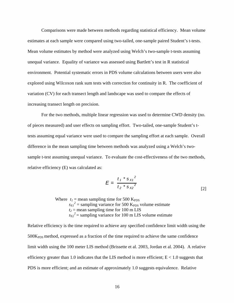
sample t-test assuming unequal variance. To evaluate the cost-effectiveness of the two methods,

relative efficiency (E) was calculated as:

[2]

t 1 * s X12

t 2 * s X22E =

Where t1 = mean sampling time for 500 KPDS sX1

2 = sampling variance for 500 KPDS volume estimate t2 = mean sampling time for 100 m LIS sX2

2 = sampling variance for 100 m LIS volume estimate Relative efficiency is the time required to achieve any specified confidence limit width using the

500KPDS method, expressed as a fraction of the time required to achieve the same confidence

limit width using the 100 meter LIS method (Brissette et al. 2003, Jordan et al. 2004). A relative

efficiency greater than 1.0 indicates that the LIS method is more efficient; E < 1.0 suggests that

PDS is more efficient; and an estimate of approximately 1.0 suggests equivalence. Relative

16

efficiency provides comparison of the methods while recognizing that PDS and LIS both provide

estimates of CWD volume at a given point, not a measure of accuracy, and as such, the

comparison incorporates the sampling errors of each method.

Monitoring approaches for detecting change in CWD attributes are most efficiently

designed by re-sampling permanently established sample points (Marshall et al. 2003). In

addition to marking each sample point, the ends of, or additionally locations at set intervals

along, transects should be permanently established (Marshall et al. 2003). To develop

monitoring recommendations, power analysis for two-tailed, one-sample t-test were performed in

R statistical environment. The standard deviation from the different LIS transect lengths and

landscapes were used to determine the sample size required on average to detect a given change

in CWD volume—given predefined alpha and power levels. Though post-hoc power analysis is

not recommended for determining the power of a study, a priori power analysis provides an

effective means of comparing the sensitivity of methods for detecting change in mean CWD

volume across a landscape. For a specified alpha level and standard deviation, either sample

size, delta (true difference in means), or power is solved by specifying the other parameters.

2.3.2. Site Effects on CWD volume

For a given landscape, the site attributes of interest were productivity, species

composition, ecological stage, and harvest history. To minimize variance due to sampling

methods, analysis of the effects of each factor on CWD volume was performed using the LIS

method with the largest sample area: 100 m LIS and 50 m LIS for the managed and old growth

landscapes, respectively. Appropriate statistical analysis approaches were chosen to assess the

affects of each attribute based on the distribution of volume estimates across factors, examined

17

using exploratory statistics (e.g., boxplots, qq plots, Bartlett’s analysis for homogeneity of

variance, and Shapiro-Wilk’s test of normality). Where appropriate, estimates were transformed

to enable parametric approaches. Conversely, nonparametric procedures were used where

parametric assumptions were violated. Differences between means for factors were detected

using the least significant difference (LSD) approach. Though this technique does not control

the experiment-wise error rate, it is more sensitive at detecting true differences given that power

is preserved. The unbalanced nature of the data and the lack of control/blocking prevented

further statistical analyses, and thus, may have limited the power of our analyses.

.

2.3.3. Comparison of CWD Attributes by Landscape

Sampling methods were modified between the managed and the old growth landscapes to

adequately address project objectives. As previously discussed, more samples were collected in

the managed landscape than the old growth in order to capture the higher anticipated spatial

variance in CWD volume. For similar reasons, only 50 meter LIS transects were used at all

sample points in the old growth landscape. Field crew travel costs were also prohibitively high,

necessitating the reduction in sample size (n=50). To minimize sampling affects on the

comparison of CWD attributes, the data set from the managed landscape was randomly subset to

replicate the sampling approach in the old growth landscape (LIS length and sample size and

spacing). Comparisons between landscapes representing different management histories were

then performed for mean coarse woody debris volume, and the distribution of this volume across

diameter and decay classes.

18

3. Results:

3.1. Comparison of CWD Methods

Across the managed landscape, there was not a significant difference between the

average sampling costs required for the two CWD methods, with a mean sampling time of 23.2

minutes for 100-meter LIS and 25.4 minutes per sample for the 500 KPDS method (Welch’s p =

0.45). LIS and PDS also exhibited similar time costs at the sample level (p = 0.46, df = 34), and

the required sampling time was not user-dependent for either method. However, sampling costs

for LIS (r2=0.47) were more strongly related to the number of pieces sampled than for PDS

(r2=0.12) (Figure 1). Despite the apparent equivalence in costs, the required time per sample was

much more variable for PDS (st= 14.8 minutes) than for LIS (st= 7.9 minutes) (Bartlett’s p <

0.001). The low correlation between sampling cost and the number of pieces sampled using the

PDS method was largely due to the extensive search radius required at most sample points.

Across stand types, visual obstruction from dense understory brush and/or regeneration

prevented initial tallies of “in” logs from the sample point and necessitated the use of a

standardized search approach. Determining the point of perpendicularity was rapid for small

logs at close distances but doing so for large logs at further distances was problematic. As

anticipated, the frequency of logs tallied using the 500KPDS factor decreased with increasing

distance from the sample point; however, logs greater than 20 meters from the sample point were

not uncommon, with the furthest recorded at approximately 40 meters (Fig. 2). Given the large

search radii required at most sample points, often there was not a clear sense of progression or

confidence of completion for the user.

Comparing mean volume estimates at each sample, there was not a significant difference

between the 250 KPDS factor and all LIS transect lengths. However, the 500KPDS factor

19

significantly underestimated volume compared to LIS transect lengths of 40, 60, 80, and 100

meters, while a significant difference from 20 meter transects was not detected. Generally, PDS

appeared to underestimate CWD volume relative to LIS (Table 7). A significant difference

across methods was not observed in estimating mean CWD volume for the managed landscape

(Table 8, Fig. 2). Although not controlling for environmental factors such as stand type and

ecological stage, an overall systematic bias between users in PDS volume estimates for both

factors was not suggested (250KPDS: W=1251.5, p = 0.83; 500KPDS: W=1295.5, p=0.60, Mann-

Whitney tests).

Sample variance was high for both methods at all levels but was reduced by increasing

the sample area—increasing LIS transect length or decreasing the KPDS volume factor (increasing

inclusion probability) (Table 8). Overall, PDS performed poorly, capturing variance (CV) only

slightly better than 20 meter LIS transects. Although the methods exacted similar sampling costs

at the sample and landscape levels, disparity between the approaches was best discerned by the

relative efficiency, where PDS (500 KPDS) was substantially less cost-effective than LIS (100m)

(E = 1.69).

For the LIS method, similar trends were observed with increasing transect length in the

two landscapes: sample variance decreased with increasing transect length (Table 9). The rate of

decrease in CV was greatest across short transect lengths in both sites—10m-30m and 10m-20m

in the managed and old growth landscapes, respectively (Fig. 4). For each respective transect

length, the CV was lower for the old growth than the managed landscape (Fig. 4). Increasing

transect length decreased CV more rapidly in the old growth than in the managed landscape

(Figure 4). The relative statistical efficiency gained by increasing LIS transect length was

marginal between 80m to 100m in the managed landscape; however, CV continued to decline

20

with increasing transect length to 50 meters in the old growth (Fig. 4). Increasing the transect

length further decreased the range of volume estimates and reduced the number of 0 m3ha-1

estimates—which were not observed with transects 40 meters or greater in the managed site and

20 meters or greater in the old growth site (Tables 8 and 9).

Based on the observed standard deviations by LIS sample area, power analysis revealed

substantial tradeoffs between sample area, sample effort, and sensitivity to change for CWD

volume in a given landscape (Fig. 5 and 6). The minimum sample size required on average to

detect a specified change in the mean CWD volume can be reduced by either decreasing the

probability of failing to reject a false null hypothesis (power) or increasing the probability of

falsely rejecting the null hypothesis when it is indeed true (alpha). The statistical constraints of

an inventory have a substantial impact on the minimal required sample effort for each landscape.

An important trend is that selection of the appropriate LIS transect length largely depends on the

true difference in mean CWD volume that a land manager desires to detect at and with what

precision. When small changes in CWD volume must be detected, efficiencies are gained by

using longer transect lengths. In such scenarios, 20 meter transects appear impractical in the

managed landscape, as do 10 meter transects in both landscapes. However, the difference in the

required sample size between longer and shorter transect lengths becomes less apparent as

restrictions are relaxed as to how large of a change in CWD volume must be detected. Though

these trends hold in the old growth landscape, it is further apparent that detecting changes in

CWD volume with high statistical power in such forests will require substantially more effort

than in the managed landscape.

21

3.2. Effects of Site Attributes on CWD Volume

Examining site attribute effects on CWD volume, our study generally failed to detect a

significant and consistent pattern across attributes and/or landscapes. One-way ANOVA

analysis of site productivity effects in the managed landscape were not significant (F= 1.83, p =

0.17). In the old growth landscape, however, there was a significant difference in the median

CWD volume across productivity classes (Kruskal-Wallis rank sum test H = 14.76, p < 0.001).

Pair-wise comparisons using Wilcoxon rank sum tests did not indicate a significant difference in

median CWD volume between medium and high productivity sites (W=127, p=0.61); although,

low productivity sites were characterized by a significantly higher median volume of CWD than

medium (W=261, p<0.001) and high (W=194, p=0.003) productivity sites. A significant

difference in the mean CWD volume for northern hardwood (Mean + SE: 52.61+4.55 m3/ha)

and spruce-fir (45.43+3.20 m3/ha) forests was not observed in the managed landscape (Welch’s

two sample t-test p = 0.20, df = 93.67). It was assumed that stand type differences would be

more apparent in the old growth landscape, where the confounding effects of management were

removed, yet this assumption was not met (Student’s two sample t-test p=0.211, df=41). As with

productivity and forest type, the median CWD volume was not significantly different across

ecological stages in the managed landscape (H=0.86, p=0.65).

The silviculture used in harvesting practices can greatly influence residual CWD volume

(Hansen et al. 1991, Franklin et al. 2002). Broadly classifying silvicultural treatments, the

number of sample points was approximately balanced between stands partially harvested

(n = 33) and clearcut (n = 31) in the last twenty-years. The distribution of volume estimates

exhibited dissimilarity by harvest type, with partially harvested stands exhibiting much greater

spread (Kolmogorov Smirnov D = 0.35, p = 0.03). Overall, partially harvested stands

22

(Mean+SE: 59.54+5.75 m3/ha) had a significantly greater mean CWD volume than clearcut

stands (48.87+ 5.48 m3/ha) (Welch two-sample t-test p = 0.05, df = 62).

3.3. Comparison of CWD Attributes by Landscape

Confounding variables likely limited our ability to interpret factors correlated with CWD

volume within landscapes; however, examining CWD attributes at larger spatial scales more

clearly revealed the possible implications of management. With lower than half the mean

volume of CWD, the managed landscape (Mean+SE 48.31+4.69) had substantially less downed

wood than the old growth (112.66+8.13 m3/ha) (Welch’s two sample p < 0.001, df=78.38). As

previously noted, the spatial distribution of CWD volume was much more variable in the

managed landscape (CV = 68%) than in the old growth (CV = 51%). The distribution of this

volume across size-classes differed between the two landscapes (Fig. 8). The mean volume of

CWD in the two smaller size classes was greater for the old growth (both p<0.001). Although,

the managed landscape had a greater proportion of its volume in the smallest size class (8-20

cm), the old growth site had a greater proportion of CWD volume in 20-40 cm logs. There was

not an apparent difference in the volume of CWD in 40-60 cm logs (p = 0.28). Logs over 60 cm

made up a greater proportion of CWD volume in the old growth, but logs over 50 cm were not

observed in the managed landscape. The distribution of CWD volume by decay class was

suggested similar trends between the landscapes (Figure 9). More CWD was in lower decay

stages (1-2) in the managed landscape than in the old growth. Generally, CWD in later decay

stages was rare in both systems.

23

4. Discussion:

4.1. Monitoring Recommendations for CWD in Northeastern Forests

In selecting the appropriate methods for structuring large-scale forest inventory and

monitoring approaches for CWD, multiple factors should be addressed—many of which are

project specific (e.g., budgetary constraints). Probably universal is the need to maximize the

statistical efficiency attained for a given cost by selecting the appropriate sampling method,

sampling area (ie. line length, KPDS factor), and sample size, all of which invoke tradeoffs.

Various studies have examined costs (e.g., Hazard and Pickford 1983) and cost-effectiveness of

LIS and alternative CWD sampling techniques (Bailey 1970, Howard and Ward 1972, Martin

1976, Delisle et al. 1988, Ståhl and Lamas 1998, Nemec and Davis 2002, Bebber and Thomas

2003, Brissette et al. 2003, Jordan et al. 2004). However, these comparisons are confined to the

stand level, and to our knowledge, none review the cost-effectiveness of PDS and LIS for large-

scale inventories and through field based assessment. Williams and Gove (2003) propose that

PDS should be the most cost-effective of the methods, requiring one-half to one-sixth the time to

achieve equivalent precision with LIS, citing preliminary field trials in the northeastern, U.S.

Supporting this claim, field studies using Point Relascope Sampling (PRS)—a complementary

plot-less approach having CWD selection probability proportional to length squared—indicated

that variable radius sampling approaches exact less time cost and are more cost-effective than

LIS (Brissette et al. 2003, Jordan et al. 2004).

Many of these comparisons are invalidated by unrealistic assumptions not met in our

study nor likely to be met in managed landscapes in the Northeast. Brissette et al. (2003)

assumed that the number of CWD pieces sampled for PRS and LIS was directly and equivalently

related to sampling time and further used a hybrid sampling approach with four 20-m LIS

24

transects arranged in a cross. Jordan et al. (2004) implemented a single LIS transect of 40.25

meters with random orientation—an inefficient approach warranting caution (Hazard and

Pickford 1986). More so, simulation studies by Williams and Gove (2003) and Bebber and

Thomas (2003) standardized sample effort across methods by equalizing the number of CWD

pieces sampled—an assumption lacking merit in field applications. Caution must be used in

comparing our results with such studies where different methods and effort (e.g., sample area,

spacing, arrangement, CWD size-restrictions) were evaluated at higher spatial resolution (within

stands vs. across stands) and in different geographic regions with varying management histories.

When sighting conditions are poor and where a large search radius is required, a high potential

for non-detection bias has been recognized with search-based approaches (Ringvall and Ståhl

1999, Bebber and Thomas 2003, Williams and Gove 2003, Jordan et al. 2004). In the managed

landscape, site limitations due to dense understory vegetation, high stocking levels, and/or large

volumes of downed wood across a range of size classes imposed greater sampling costs for PDS

than expected.

With large-scale inventories, cost evaluation must extend beyond sampling time. For

instance, the increased discrepancy between LIS and PDS volume estimates with increasing PDS

factor (theoretical search radius) may have been due to a consistent non-selection bias across

users. The absence of significant differences in the volume estimates and sample costs for both

methods according to user, however, suggests that such systematic biases were unlikely.

Theoretically, PDS demands much lower sampling costs because only borderline logs must be

measured. Under the field conditions observed in our study, such assumptions were invalid.

Rarely were logs easily distinguished as “in” due to the previously mentioned constraints. The

lack of a clear sense of progression and survey completion with PDS may result in decreased

25

crew morale and enhanced fatigue, propagating further user errors. Surveys based solely on

ocular estimation of “in” logs and measurement of borderline logs with PDS may introduce

significant user biases—a non-issue in our study given the individual measurement of each CWD

piece. Although surveyor bias may also occur with the LIS method, systematic error is atypical,

despite some random measurement error, due to the more restricted protocol (Ringvall and Ståhl

1999). Under the field conditions experienced in our study, LIS provided a clearer sense of

progression and confidence in the survey method. LIS appeared more robust to measurement

error and simpler to understand and perform. Though beyond the scope of this study, re-

measurement of a subset of samples by each user using the same method would have better

revealed potential surveyor bias. Large-scale inventories should recognize and account for

surveyor based measurement errors.

The adaptability of LIS to meet specific land management needs further supports the

selection of this method. Whereas one-factor of PDS may only be used to estimate volume and

may not be extended to other CWD attributes, small adjustments to LIS sampling protocol, such

as estimating piece length, allow calculation of total and average CWD length, density, surface

area, projected area, diameter, and biomass (Marshall 2000, Marshall et al. 2003). Overall, PDS

was the least cost-effective sampling approach. From our analysis, it cannot be recommended

over LIS for large scale surveys of managed forests in the northeast, implementing a similar

sampling design and field equipment as in this study.

In using LIS for large scale inventories, land managers must determine an appropriate

transect length to capture the spatial variance of CWD. Previous studies suggest that LIS

requires substantial effort (total line length) to achieve high precision (Pickford and Hazard

1978); however, the sampling effort required differs vastly based on the characteristics of CWD

26

in the region and the statistical constraints of the inventory. Site specific factors that influence

the efficiency of different transect lengths include the spatial distribution, frequency, total

volume, size class distribution, and shape of CWD (Warren and Olsen 1964, De Vries 1973,

Pickford and Hazard 1978, Marshall 2002, Nemec and Davis 2002, Woldendorp 2004).

Accordingly, shorter transect lengths and fewer samples are required where the spatial

distribution of CWD is more homogeneous and found at higher frequencies, greater volumes,

across fewer size-classes, and exhibits less taper.

Precision of volume estimates for a landscape may be increased either by increasing the

transect length—thus decreasing the standard deviation—or expanding the sample size to

decrease the standard error of the mean. This relationship breaks down at its extremes (Pickford

and Hazard 1978, Woldendorp 2004), and consequently, extremely short transects (< 10 m) are

not recommended. Other studies have also observed the greatest decrease in CV with increasing

the length of shorter transects and a likewise reduction in the range of CWD volume estimates

(Woldendorp 2004). The lower CV for a given transect length in the old growth landscape was

attributed to higher CWD volumes and the decreased spatial heterogeneity of this volume.

Given the seemingly asymptotic trend in CV with transect lengths greater than 80 meters in the

managed landscape, this transect length is likely sufficient to capture the spatial variance of

CWD. With no such trend observed in the old growth landscape, transect lengths longer than 50

meters may be more statistically efficient where there are comparable volumes of CWD.

The decision of an appropriate transect length is project specific and largely directed by

budgetary constraints. Costs will dictate variables such as the number of samples that can be

collected in a given amount of time using a field crew of a certain size. Given the lack of

financial return from downed CWD, the most cost-effective sampling strategy for CWD volume

27

would be to integrate supplemental protocol into existing commercial inventories for standing

trees (e.g., Waddell 2001, Marshall et al. 2004). Most large-scale inventories, as such, use a

systematic random sampling design without stratification similar to that assumed in our project.

The extreme spatial variability of CWD requires a substantial sampling effort to monitor changes

in CWD volume with high precision. As such, land managers in the northeast need an idea of

the level monitoring performance they can anticipate for an allotted sampling effort.

Specifically, tradeoffs exist between the sensitivity of an approach (LIS length and sample size)

in detecting an actual change in CWD volume (power) versus the probability of indicating a

significant change when none is present (alpha). Aware of these tradeoffs upfront, land

managers may consult the appropriate graphs for the landscape most similar to their management

scenario and determine the minimum effort required on average to detect a specific change in

CWD volume. Though these calculations provide a generalized estimate of the sample effort

required, they elucidate valuable practicalities regarding the statistical efficiency of the different

LIS approaches for monitoring changes in CWD volume across a landscape. Where highly-

sensitive methods are required to detect small changes in mean CWD volume, efficiencies are

gained by using longer transects. Conversely, where detection of only larger changes in mean

CWD volume is necessary, the efficiency gained by using longer transects diminishes.

4.2. Effects of Site Attributes on CWD Volume and Management Implications

Reduction in variance and an increase in the power of an inventory to detect change is

usually attained through stratification by factors such as productivity, forest type, harvest history,

and ecological stage. However, consistent relationships to allow such stratification were not

observed in the managed and old growth landscapes. The volume of CWD is a function of

28

complex input and output process interactions at various spatial and temporal scales (Harmon et

al. 1986), which make such stratification difficult. For instance, site productivity affects species

composition, growth rates and size potential, disturbance processes, stand stocking levels, and

the rate at which stands enter stem exclusion—all of which interactively influence CWD input

and output rates (Harmon et al. 1986, Sturtevant et al. 1997). Several studies have demonstrated

greater tree mortality, CWD volume, and frequency of large downed logs with increasing site

productivity (Volk and Fahey 1994, Sturtevant et al. 1997, Spetich et al. 1999). Conversely, a

consistent trend between productivity and CWD volume was not detected in our study, even

when controlling for other factors. In the old-growth stand, however, CWD volume was greater

in low productivity sites. As classified, low productivity sites were characterized by very poorly

drained soils, which may result in increased windthrow mortality—a dominant natural

disturbance process in these forests (McCune et al. 1988, Seymour et al. 2002, Lorimer and

White 2003). Extending residence time, slow decay due to local abiotic conditions and the

cooler regional climate likely facilitates CWD accumulation. In the managed site, complex

interactions between factors, both recorded and not, likely concealed productivity effects.

Alternatively, the site productivity classification system used may have been insensitive to

significant differences in productivity, or productivity may influence CWD input at larger

geographic scales where differences are greater (Spetich et al. 1999). Similar confounding

factors may have obscured the effects of forest type. Spruce-fir forests typically exhibit higher

CWD volumes than northern hardwood stands, with the relationship generally maintained for

coniferous and deciduous forest types within the same region due to faster decay rates in the

latter forests (Harmon et al. 1986); however, no such trend was observed in either landscape.

29

Space-for-time substitution in chronosequence studies has provided an abundance of

information on how CWD volume changes with stand development. Across forest types and

following both natural and harvest disturbance, a general “U-shaped” temporal pattern has been

observed for CWD volume with stand age (Bormann and Likens 1979, Gore and Patterson 1986,

Spies and Cline 1988, McCarthy and Bailey 1994, Petranka et al. 1994, Stevens 1997, Clark et

al. 1998, Crooks et al. 1998). Following initial disturbance, stands are characterized by high

residual CWD volumes which then decrease overtime. At the stem exclusion stage, CWD

volume theoretically reaches a minimum with depletion of the residual but then begins to

increase through inputs from the current stand. Contribution from the resident stand continues

through competitive exclusion and small-scale disturbance induced mortality, reaching a

maximum at the multi-aged stage. Surprisingly, no such trend was observed between CWD

volume and ecological stage in the managed landscape, with forests exhibiting similar volumes

across ages. However, the availability of CWD during early stages of stand development is

largely dependent upon stand history (Spies and Cline 1988). Fraver et al. (2002) suggests that

the “U-shaped” temporal trend may not be applicable to selectively harvested stands in the

Acadian forests of Northern Maine due to the complex interaction of natural, small-scale

disturbances and repeat harvest entries. Numerous studies have also failed to recognize the

common “U-shaped” temporal pattern (Carleton and Arnup 1993, Goebel and Hix 1996, Busing

1998, Hardt and Swank 1997, Lee et al. 1997, Flemming and Freedman 1998). Although

chronosequence studies may reveal general trends, controlled studies over longer time scales

where CWD inputs and outputs are more closely followed (ie., pre-harvest and post-harvest

measurements) would better distinguish the effects of harvesting on CWD volume in our study

site.

30

4.3. Comparison of CWD Attributes Between the Managed and Old Growth Landscape

More generally comparing the two landscapes, substantial differences were apparent in

CWD volume and the distribution of this volume across size and decay classes, bringing into

question the effects of forest management. Although our study did not examine paired

chronosequences of forest development for managed and natural stands, many such studies have

suggested that managed forests exhibit lower accumulation of CWD across all stages of stand

development (Flemming and Freedman 1998, Duvall and Grisgal 1998, Goodburn and Lorimer

1998). Particularly strong disparities occur in the stand initiation and demographic transition

stages (Duvall and Grisgal 1989). CWD inputs from harvests are often much lower than natural

disturbances (Sippola et al. 1998), and management activities such as pre-commercial and partial

harvest often preclude natural stem mortality from stem exclusion and thus CWD accumulation

(Flemming and Freedman 1998). Harvest operations also differ in the amount of residual CWD

due to decay rates and standing tree retention: CWD decays much more rapidly after clearcutting

and partial harvests leave standing live and damaged trees to contribute to CWD inputs

(Bormann and Likens 1979, Hansen 1991). These factors most likely drive the difference in

CWD volume observed between these practices in the managed landscape.

The exact difference in CWD volume between managed and old growth stands varies

largely dependent on geographic region and forest type: in old growth sites in Indiana, Illinois,

Iowa, and Missouri, Spetich et al. (1999) found three-times the volume of downed CWD as in

second growth sites; Shifley et al. (1997) observed twice the volume of CWD in old growth than

70- and 90- years old second growth stands in Missouri; and McGee et al. (1999) recorded nearly

twice the volume of downed CWD in old growth than in mature-managed and partially harvested

northern hardwood stands. Our results correspond closely with those of McGee et al. (1999) in

31

that the mean volume of CWD in the old growth landscape was more than twice that in the

managed. Further, the mean volume of CWD in the old-growth landscape approximated McGee

et al.’s (1999) estimated average of 110 m3/ha for old growth, northern hardwood stands.

In addition to total CWD volume, forest management further effects the distribution of

this volume across diameter classes, with a reduction in the number of large-diameter logs and

large logs in advanced decay stages (Andersson and Hytteborn 1991, Hansen et al. 1991, Guby

and Dobbertin 1996, Freedman et al. 1996, Fridman and Walheim 2000). Although rare in both

sites, large logs (>50 cm) were absent from the managed landscape. Whereas Gore and

Patterson (1986) did not observe downed CWD > 38 cm in uneven-aged managed northern

hardwood stands of New Hampshire; the managed landscape, the managed landscape had nearly

the same volume of logs 40-60 cm as in the old growth. Retention of large trees and snags is

essential for biodiversity and ensuring their future contribution to the CWD pool (Hansen et al.

1991). The paucity of large logs (>60 cm) in the managed landscape suggests that current

retention of such structural features may be insufficient to emulate old-growth CWD conditions.

However, the high proportion of volume in 40-60 cm logs in the managed landscape indicates

that current harvesting practices are retaining large logs that contribute to future stands. The

implications for biodiversity will be largely affected by species assemblages and threshold

values. Further research is warranted on the topic in the Northeast.

Whereas natural disturbances contribute dead wood across size-classes, harvests result

primarily in an input of small diameter CWD (Fraver et al. 2002). Supporting this trend, the

managed landscape had a larger proportion of CWD volume in smaller diameter classes (8-20

cm) compared; however, the old growth landscape had a greater proportion of volume in

intermediately sized (20-40cm) down wood. Shifley et al. (1997) similarly observed a lower

32

proportion of volume in logs over 20 cm in managed than in old growth stands. The distribution

of CWD volume across diameter classes affects the ecological functions that CWD sustains and

thus forest biodiversity. Larger logs typically exhibit greater structural diversity, such as more

frequent and larger cavities which provide microsites used by a diversity of animals for denning

and shelter (Harmon et al. 1986). Some small mammal species preferentially inhabit logs of

different diameters (Hayes and Cross 1987), and many bryophyte speices are large-log

specialists. The greater distribution of CWD volume across size classes in the old growth stand

likely provides a diversity of microsites for species; whereas, conversely the declining

distribution of CWD volume with log size in the managed landscape may not provide adequate

structural diversity for many wood-dependent species.

Another factor affecting the functional value of dead wood for forest biodiversity is the

distribution of CWD volume across decay classes. As dead wood structurally changes through

decay, so does its functional role as habitat for different species. A successional transition of

bryophyte (Andersson and Hytteborn 1991; Rambo and Muir 1998), fungi, and invertebrate

communities has been observed or suggested with wood decay states (Crites and Dale 1998).

CWD decay state further affects which vertebrate species use logs and in what manner (Thomas

1979). Therefore, the greatest diversity is supported through distribution of CWD volume across

decay classes. As such, the higher proportion of log volume in early decay stages may diminish

the ecological value of CWD in the managed landscape relative to the old growth site. The

larger proportion of volume in the most decayed state for the managed landscape was likely due

to the correlation between size and decay—smaller logs in the managed landscape decay more

rapidly. Various other factors, such as how decay is distributed across size classes, species,

forest types, and forest connectivity, influence the functional role of CWD. Therefore, these

33

attributes provide a generalized perspective of how landscapes may differ due to management

practices.

4.4. Considerations in Applying and Extending Project Results

Although these results provide general recommendations of how land managers might

effectively monitor changes in CWD volume in northeastern forests and furthermore reveal

insights into how CWD attributes vary between a managed and old growth landscape, several

caveats must be acknowledged. Concerning the LIS method, orientation bias, in which logs are

not randomly oriented, has been recognized as inducing significant bias in volume estimates

(Warren and Olsen 1964, van Wagner 1968, De Vries 1979, Hazard and Pickford 1986).

Consequently, various arrangements of transects have been used and suggested to be more

efficient—such as running two lines in random directions (van Wagner 1968, Howard and Ward

1972), three or five transects radiating from a central point (e.g., Waddell 2002, Nemec and

Davis 2002), and an equilateral triangle (e.g., Delisle et al. 1988). Despite their wide use, the

bias and variance properties of such hybrid methods have only recently been examined (Affleck

et al. 2005, Barbesi 2007). When CWD pieces are randomly oriented, there is no advantage in

using one arrangement over the other (Bell et al. 1996, Nemec and Davis 2002, Woldendorp et

al. 2004). Furthermore, such approaches may exact greater sampling costs, and a single line

would, in most cases, better capture the spatial variance of CWD (Marshall 2002). Though

significant departures from random orientation were not observed in the field, non-random

orientation may be difficult to detect. It must then be acknowledged that the fixed orientation of

LIS transects in our study may have induced increased variance in volume estimates, not

negating the methods comparisons but with potential implications for the power analysis.

34

The LIS approach used assumes that logs are intersected at their midpoint on average.

This assumption may have introduced inaccuracy in our comparison of volume distribution

across size-classes. Though beyond the scope of our study given that land mangers would

generally only be interested in CWD volume, more accurate estimates could have been attained

by measuring additional variables, such as piece length, midpoint, small and large end diameters.

The analyses presented are limited to static observations and must be interpreted as such.

General trends are presented regarding the distribution of volume across size- and decay-classes

due to the inherent variability in these attributes and the difficulty of attaining precise estimates

(Shifley et al. 1994). CWD volume is affected by a complex of factors that impact temporal and

spatial patterns through input and output processes. Though both sites exhibited similar forest

types and abiotic conditions, with management history the most prominent difference, the limited

temporal scale of the study and the inability to account, nigh control for, all variables must be

recognized. Further research is needed surrounding the biotic and abiotic interactions—and the

relavent spatial scales of these processes—that affect the biodiversity support function of CWD

in the Northeast.

35

5. Literature Cited

Affleck, D.L.R., Gregoire, T.G., and H.T. Valentine. 2005. Design unbiased estimation in line intersect sampling using segmented transects. Environmental and Ecological Statistics 12: 139-154.

American Forest & Paper Association, Inc. 2005. Sustainable Forestry Initiative Standard (SFIS): 2005-2009 Standard. Accessed 5 July 2007. <http://www.aboutsfi.org/documents/SFIStandard2005-2009_002.pdf.

Andersson, L.I. and H. Hytteborn. 1991. Bryophytes and decaying wood—a comparison between managed and natural forest. Holarctic Ecology 14:121-130.

Barbesi, L. 2007. Some comments on design-based line-intersect sampling with segmented transects. Environmental and Ecological Statistics 14: 483-494.

Beatty, S.W. and E.L. Stone. 1986. The variety of soil microsites created by tree falls. Can. J. For. Res. 16: 539-548.

Bebber, D.P. and S.C. Thomas. 2003. Prism sweeps for coarse woody debris. Canadian Journal of Forest Research 33: 1737-1743.

Bell, G., Kerr A., McNickle, D., and R. Woollons. 1996. Accuracy of the line intersect method of post-logging sampling under orientation bias. Forest Ecology and Management 84: 23-28.

Berg, A., Ehnstrom, B., Gustafsson, L, Hallinback, T, Jonsell M., and J. Weslien. 1994. Threatened plant, animal, and fungus species in Swedish forests: distribution and habitat associations. Conservation Biology 8(3): 718-731.

Bormann, F.H. and G.E. Likens. 1979 . Pattern and Process in a Forested Ecosystem. New York: Springer Verlag. 262 p.

Briggs, R.D. 1994. Site classification field guide. Maine Agricultural Forestry Experiment Station Mis. Publ. 724.

Brissette, J.C., Ducey, M.J., and J.H. Gove. 2003. A field test of point relascope sampling of down coarse woody material in managed stands in the Acadian forest. Journal of the Torrey Botanical Society 130(2): 79-88.

Brown, J.K. 1971. A planar intersect method for sampling fuel volume and surface area. Forest Science 17: 96-102.

Brown, J.K. and P.J. Roussopoulos. 1974. Eliminating biases in the planar intersect method for estimating volumes of small fuels. Forest Science 20: 350-356.

Busing, R.T. 1998. Structure and dynamics of cove forests in the Great Smoky Mountains. Castanea 63: 361-371.

Canfield, R.H. 1941. Application of the line interception method in sampling range vegetation. Journal of Forestry 39(4): 388-394.

Carleton, T.J. and R.W. Arnup. 1993. Vegetation ecology of eastern white pine and red pine forests in Ontario. Forest Fragmentation and Biodiversity Project Report No. 11. Ontario Forest Research Institute.

Chokkalingam, U. and A. White. 2000. Structure and spatial patterns of trees in old-growth northern hardwood and mixed forests of northern Maine. Plant Ecology 00: 1-22.

Clark, D.F., Kneeshaw, D.D., Burton, P.J., and J.A. Antos. 1998. Coarse woody debris in sub-boreal forests of west-central British Columbia. Canadian Journal of Forest Research 28: 284-290.

36

Crooks, J.B., III, Waldrop, T.A., Van Lear, D.H., and V.B. Shelburne. 1998. Dynamics of coarse woody debris in unmanaged piedmont forests as affected by site quality. In T.A. Waldrop (ed.). Proceedings of the ninth biennial southern silvicultural research conference. USDA For. Serv. Gen. Tech. Rep. SRS-20. 473-477.

De Vries, P.G. 1973. A general theory on line intersect sampling with applications to logging residue inventory. Mededelingen Landbouwhogeschool Wageningen 73(11): 1-23.

DeGraff, R.M. and D.D. Rudis. 1986. New England Wildlife: habitat, natural history, and distribution. 1986. General Technical Report. NE-108, Newton Square, PA: Northeast Research Station, USDA Forest Service. 27 p.

Delisle, G.P., Woodard, P.M., Titus, S.J., and A.F. Johnson. 1988. Sample size and variability of fuel weight estimates in natural stands of lodgepole pine. Canadian Journal of Forest Research 18: 649-652.

Duvall, M.D. and D.F. Grisgal. 1999. Effects of timber harvesting on coarse woody debris in red pine forests across the Great Lakes states, USA. Canadian Journal of Forest Research 15: 914-921.

Esseen, P. and K. Reinhorn. 1996. Epiphytic lichen biomass in managed and old-growth boreal forests: effect of branch quality. Ecological Applications 6(1): 228-238.

Flemming, T.L. and B. Freedman. 1998. Conversion of natural, mixed-species forest to conifer plantations: implications for dead organic matter and carbon storage. Ecoscience 5: 213-221.

Franklin, J.F., Shugart, H.H., and M.E. Harmon. 1987. Tree death as an ecological process. BioScience 37(8): 550-556.

Fraver, S., Wagner, R.G., and M. Day. 2002. Dynamics of coarse woody debris following gap harvesting in the Acadian forest of central Maine, U.S.A. Canadian Journal of Forest Research 32: 2094-2105.

Freedman, B., Zelanzy,V., Beaudette, D, Fleming T., Johnson G., Flemming S., Gerrow J.S., Forbes G., and S. Woodley. 1996. Biodiversity implications of changes in the quantity of dead organic matter in managed forests. Environmental Review 4(3): 238-265.

Fridman, J. and M. Walheim. 2000. Amount, structure, and dynamics of dead wood on managed forestland in Sweden. Forest Ecology and Management 131: 23-36.

Goebel, P.C. and D.M. Hix. 1996. Development of mixed-oak forest in southeastern Ohio: a comparison of second-growth and old-growth forests. Forest Ecology and Management 84: 1-21.

Gore, J.A. and W.A. Patterson. 1986. Mass of downed wood in northern hardwood forests in New Hampshire, potential effects of forest management. Canadian Journal of Forest Research 16: 335-339.

Gove, J.H., Ringvall, A., Ståhl, S., and M.J. Ducey. 1999. Point relascope sampling of downed woody debris. Canadian Journal of Forest Research 29: 1718-1726.

Hagan, J.M. and S. Grove. 1999. Coarse woody debris: humans and nature competing for trees. Journal of Forestry 97(1): 6-11.

Hansen, A.J., Spies, T.A., Swanson, F.J., and J.L. Ohmann. 1991. Conserving biodiversity in managed forests. BioScience 41(6): 382-392.

Hanski, I. 2000. Extinction debt and species credit in boreal forests: modeling the consequences of different approaches to biodiversity conservation. Ann. Zool. Fennici 37: 271-280.

37

Hardt, R.A. and W.T. Swank. 1997. A comparison of structural and compositional characteristics of southern Appalachian young second-growth, maturing second-growth, and old-growth stands. Natural Areas Journal Assessment of coarse woody debris: a comparison of probability sampling methods 17: 42-52.

Harmon, M.E. and C. Hua. 1991. Coarse woody debris dynamics in two old-growth ecosystems. BioScience 41(9): 604-610.

Harmon, M.E., Franklin, J.F., Swanson, F.J., Sollins, P., Gregory, S.V., Lattin, J.D., Anderson, N.H., Cline, S.P., Aumen, N.G., and J.R. Seddell. 1986. Ecology of Coarse Woody Debris in Temperate Ecosystems. Advances in Ecological Research 15: 133-302.

Harmon, M.E., Karnkina, O.N., Yatskov, M, and E. Mathews. 2001. Predicting broad-scale carbon stores of woody detritus from plot-level data. In: Lai, R., Kimble, J., and B.A. Stewart. Assessment methods for soil carbon. New York: CRC Press, 533-552.

Hayes, J.P. and Cross, S.P. 1987. Characteristics of logs used by western red-backed voles, Clethrionomys californicus, and deer mice, Peromyscus maniculatus. Can. Field-Nat. 101: 543-546.

Hazard, J.W. and S.G. Pickford. 1983. Cost functions for the line intersect method of sampling forest residue in the Pacific Northwest. Canadian Journal of Forest Research 14: 57-62.

Hazard, J.W. and S.G. Pickford. 1986. Simulation studies on line intersect sampling of forest residue. Part II. Forest Science 32: 447-470.

Helms, J.A. 1998. “The Dictionary of Forestry.” Society of American Foresters: Bethesda, MD. 210 p.

Howard, J.O. and F.R. Ward. 1972. Measurement of logging residue—alternative applications of the line intersect method. USDA Forest Service Research Note PNW-183, 8 p.

Hunter, M.L. 1990. Wildlife, Forests and Forestry: Principles of Managing for Biological Diversity. Prentice-Hall, New Jersey.

Jordan, G.J., Ducey, M.J., and J.H. Gove. 2004. Comparing line-intersect, fixed-area, and point relascope sampling for dead and downed coarse woody material in a managed northern hardwood forest. Canadian Journal of Forest Research 34: 1766-1775.

Jurgensen, M.F., Harvey, A.E., Graham, R.T., Page-Dumroese, D.S., Tonn, J.R>, Larsen, M.J., and T.B. Jain. 1997. Impacts of timber harvesting on soil organic matter, nitrogen productivity, and health of inland northwest forests. Forest Science 43: 234-251.

Kaiser, L. 1983. Unbiased estimation in line-intersect sampling. Biometrics 39(4): 965-976. Keddy, P.A. and C.G. Drummond. 1996. Ecological properties for the evaluation, management,

and restoration of temperate deciduous forest ecosystems. Ecological Applications 6(3): 748-762.

Lee, P.C., Crites, S., Nietfeld, M., Van Nguyen, H., and J.B. Stelfox. 1997. Characteristics and origins of deadwood material in aspen-dominated boreal forests. Ecological Applications 7: 691-701.

Lesica, P., McCune, B., Cooper, S.V., and W.S. Hong. 1991. Difference in lichen and bryophyte communities between old-growth and managed second-growth forests in the wan Valley, Montana. Canadian Journal of Botany 69: 1745-1755.

Lindenmayer, D.B., Margules, C.R., and D.B. Botkin. 2000. Indicators of biodiversity for ecologically sustainable forest management. Conservation Biology 14(4): 941-950.

Lorimer, C.G. and A.S. White. 2003. Scale and frequency of natural disturbances in the northeaster US: implications for early successional forest habitats and regional age distributions. Forest Ecology and Management 185: 41-64.

38

Marie-Josee, S., Yves, B., and L. SIrois. 1998. Conifer seedling recruitment in a southeastern Canadian boreal forest: the importance of substrate. Journal of Vegetation Science 9: 575-582.

Marshall, P.L. Davis, G., and S.W. Taylor. 2003. Using line intersect sampling for coarse woody debris: practitioners’ questions addressed. Forest Research Extension Note. V9T, 6E9, 250-751-7001, Nanaimo, BC: Coast Forest Region. 10 p.

Marshall, P.L., Davis, G., and V.M. LeMay. 2000. Using line intercept sampling for coarse woody debris. Forest Research Technical Report. TR-003, Nanaimo,BC: Vancouver Forest Region. 37 p.

Martin, A.J. 1976. Suitability of the line intersect method for sampling hardwood logging residues. USDA Forest Service Research Paper NE-339. 6 p.

Maser, C., Mate, B.R., Franklin, J.F. and C.T. Dyrness. 1979. Dead and down woody material. In: Wildlife Habitats in Managed Forests, the Blue Mountains of Oregon and Washington. USDA For. Serv. Agric. Handb. 553, Washington Off., Washington, D.C.

McCarthy, B.C. and D.R. Bailey. 1996. Composition, structure, and disturbance history of Crabtree Woods: an old-growth forest in western Maryland. Bulletin of the Torrey Botanical Club 123: 350-365.

McCune, B., Cloonan, C.L., and T.V. Armentano. 1998. Tree mortality and vegetation dynamics in Hemmed Woods, Indiana. American Midlands Naturalist 120: 416-431.

McGee, G.G., Leopold, D.J., and R.D. Nyland. 1999. Structural characteristics of old-growth, maturing, and partially cut northern hardwood forests. Ecological Applications 9(4):1316-1329.

McWilliams, W.H., Butler, B., Caldwell, L., Griffith, D., Hoppus, M., Laustsen, K., Lister, A., Lister, T., Metzler, J., Morin, R., Sader, S., Stewart, L., Steiman, J., Westfall, J., Williams, D, Whitman, A., and C. Woodall. 2003. Forests of Maine. USDA Forest Service. NE Experimental Station, Resource Bulletin.

Nemec, A.F.L. and G. Davies. 2002. Efficiency of six line intersect sampling designs for estimating volume and density of coarse woody debris. Forest Research Technical Report. TR-021, Nanaimo, BC: Vancouver Forest Region. 37 p.

Niemela, J. 1997. Invertebrates and boreal forest management. Conservation Biology 11(3): 601-610.

Northeast Region Working Group. “Forest Stewardship Standard for the Northeast Region.” 10 October 2005. Accessed 5 July 2007. <http://www.fscus.org/ images/documents/2006_standards/ne_9.0_NTC.pdf>

Noss, R.F. 1999. Assessing and monitoring forest biodiversity: a suggested framework and indicators. Forest Ecology and Mgmt. 115: 135-146.

Oliver, C. and B. Larson 1996. Forest Stand Dynamics, second ed. McGraw-Hill, Inc., New York.

Petranka, J.W., Brannon, MP., Hopey, M.E., and C.K. Smith. 1994. Effects of timber harvesting on low elevation populations of southern Appalachian salamanders. Forest Ecology and Management 67: 135-147.

Pickford, S.G. and J.W. Hazard. 1978. Simulation studies on line intersect sampling of forest residue. Forest Science 24: 469-483.

Pyle, C. and M.M. Brown. 1998. A rapid system of decay classification for hardwood logs of the eastern deciduous forest floor. Journal of the Torrey Botanical Society 125(3): 237-245.

39

Pyle, C. and M.M. Brown. 1999. Heterogeneity of wood decay classes within hardwood logs. Forest Ecology and Management 114: 253-259.

Rambo, T.R. and P.S. Muir. 1998. Bryophyte species associations with coarse woody debris and stand ages in Oregon. The Bryologist 10(3): 366-376.

Ringvall, A. and G. Ståhl. 1999. On the field performance of transect relascope sampling for assessing downed coarse woody debris. Scandinavian J. of For. Res. 14(6): 552-557.

Ringvall, A. and G. Ståhl. 1999. Field aspects of line intersect sampling for assessing coarse woody debris. Forest Ecology and Management 24: 469-483.

Rothermel, R.C. 1972. A mathematical model for predicting fire spread in wildland fuels. USDA For. Serv. Res. Paper INT-115.

Samuelsson, J., Gustafsson, L., and T. Ingeloeg. 1994. Dying and dead trees: a review of their importance for biodiversity. Swedish Threatened Species Unit, Uppsala, Sweden. p. 109.

Selva, S.B. 1994. Lichen diversity and stand continuity in the northern hardwoods and spruce-fir forests of northern New England and Western New Brunswick. The Bryologist 97(4):424-429.

Shifley, S.R. and R.C. Schlesinger. 1994. Sampling guidelines for old-growth forests in the Midwest, USA. Natural Areas Journal 14: 258-268.

Shifley, S.R., Brookshire, B.L., Larsen, D.R., and L.A. Herbeck. 1997. Snags and down wood in Missouri old-growth and mature second-growth forest. Northern Journal of Applied Forestry 14: 165-172.

Sippola, A.L., Sittonen, J., and R. Kallio. 1998. Amount and quality of coarse woody debris in natural and managed coniferous forests near the timberline in Finnish Lapland. Scandinavian Journal of Forest Research 13(2): 204-214.

Spetch, M.A., Shifley, S.R., and G.R., Parker. 1999. Regional distribution and dynamics of coarse woody debris in Midwestern old-growth forests. Forest Science 17: 1585-1595.

Spetich, M.A., Shifley, S.R., and G.R. Parker. 1999. Regional distribution and dynamics of coarse woody debris in Midwestern old-growth forests. Forest Science 45: 302-313.

Spies, T.A. and J.F. Franklin. 1991. The structure of natural young, mature, and old-growth forests in Washington and Oregon. General Technical Report. PNW-GTR-285. Portland, OR: Pacific Northwest Research Station, USDA Forest Service. 21 p.

Spies, T.A. and S.P. Cline. 1988. Coarse woody debris in forests and plantations of coastal Oregon. In C. Maser, R.F. Tarrant, J.M. Trapp, and J.F. Franklin (eds.). From the forest to the sea: A study of fallen logs. USDA For. Serv. Gen. Tech. Rep. PNW-GTR-229: 5-24.

Ståhl, G. 1998. Transect relascope sampling—a method for the quantification of coarse woody debris. Forest Science 44(1): 58-63.

Ståhl, G. and T. Lamas. 1998. Assessment of coarse woody debris: a comparison of probability sampling methods. In P. Bachmann, M. Kohl, and R. Paivinen (eds). Assessment of Biodiversity for Improved Forest Planning. European Forest Institute Proceedings 18: 241-248.

Ståhl, G. Ringvall, A., and J. Fridman. 2001. Assessment of coarse woody debris—a methodological overview. Ecological Bulletins 49: 57-70.

Stevens, V. 1997. The ecological role of coarse woody debris: an overview of the ecological importance of CWD in BC forests. Working Paper No. 30. Ministry of Forests Research Program, British Columbia.

40

Sturtevant, B.R., Bissonette, J.A., Long, J.N., and Roberts, D.W. 1997. Coarse woody debris as a function of age, stand structure, and disturbance in boreal Newfoundland. Ecological Applications 7: 702-712.

Swanson, F.J. and J.F. Franklin. 1992. New forestry principles from ecosystem analysis of Pacific Northwest forests. Ecological Applications 2(3): 262-274.

Symour, R.S., White, A.S., and P.G. deMaynadier. 2002. Natural disturbance regimes in northeastern North America—evaluating silvicultural systems using natural scales and frequencies. Forest Ecology and Management 155: 357-367.

Thomas, J.W. 1979. Wildlife habitats in managed forests, the Blue Mountains of Oregon and Washington. USDA For. Serv. Agric. Handb. 553. Washington Off., Washington, D.C. 512 p.

Tinker, D.B. and D.H. Knight. 2001. Temporal and spatial dynamics of coarse woody debris in harvested and unharvested lodgepole pine forests. Ecological Modelling 141: 125-149.

Tubbs, C.H., DeGraaf, R.M., Yamasaki, M., and W.M. Healy. 1987. Guide to wildlife tree management in New England northern hardwoods. General Technical Report. NE-118, Newton Square, PA: Northeast Research Station, USDA Forest Service. 34 p.

Turner, M.G., Romme, W.H., and D.B. Tinker. 2003. Surprises and lessons from the 1988 Yellowstone fires. Frontiers in Ecology and the Environment 1(7): 351-358.

Van Wagner, C.E. 1968. The line intersect method for forest fuel sampling. Forest Science 14: 20-26.

Van Wagner, C.E. 1968. The line intersect method in forest fuel sampling. Forest Science 14: 20-26.

Volk, T.A. and T.J. Fahey. 1994. Fifty-three years of change in an upland forest in south central New York: growth, mortality, and recruitment. Bulletin of the Torrey Botanical Club 121: 140-147.

Waddell, K.L. 2002. Sampling coarse woody debris for multiple attributes in extensive resource inventories. Ecological Indicators 1: 139-153.

Warren, W.G. and P.F. Olsen. 1964. A line intersect technique for assessing logging waste. Forest Science 10(3): 267-276.

Warren, M.S., and R.S. Key. 1991. Woodlands: past, present, and potential for insects. In N.M. Collins and J.A. Thomas, eds. The Conservation of Insects and their Habitats. Academic Press, London, UK. 155-211.

Whitman, A.A. and J.M. Hagan. 2007. An index to identify late-successional forest in temperate and boreal zones. Forest Ecology and Mgmt. 246: 144-154.

Williams, M.S. and J.H. Gove. 2003. Perpendicular distance sampling: an alternative method for sampling downed coarse woody debris. Canadian Journal of Forest Research 33:1564-1579.

Williams, M.S., Ducey, M.J., and J.H. Gove. 2005. Assessing surface area of coarse woody debris with line intersect and perpendicular distance sampling. Canadian Journal of Forest Research 35: 949-960.

Woldendorp, G., Keenan, R.J., Barry, S., and R.D. Spencer. 2004. Analysis of sampling methods for coarse woody debris. Forest Ecology and Management 198: 133-148.

41

Table 1. Classification system for CWD decay from Hunter (1990), as adapted by Maser et al. 1979 and Thomas et al. 1979 from Fogel et al. 1973.

Decay Classes1 Bark firmly attached, exposed wood has fresh color (not weathered),

wood beneath bark is solid, small twigs and branches intact, log elevatedon support point/branches.

2 Bark flaking, not firmly attached, bare wood has weathered appearance,kicking the log may knock off bark but wood is solid, small twigs mostly absent, larger branches mostly intact, log elevated but may sag slightly.

3 Bark mostly absent, surface of bare wood will flake off or shred when kicked, log is firm but some areas of the wood are soft when pressed witha foot, large branches mostly absent, log sagging considerably, much of it is on the ground.

4 Log no longer solid and intact piece, log will crush or break into large pieces when kicked, log shape becoming oval or flattened, wood is very softwhen pressed with finger, powder wood may be present, nearly all of log on the ground.

5 Log oval or flat, enerally powder wood, log very soft, can be easily brokenusing your fingers, entire log is on the ground.

6 Decomposed log forms a ridge on forest floor, is uaully fully covered with moss, organic material, seedlings, etc., digging into ridge reveals remnants of powder wood beneath organic matter and soil.

Key Characteristics

Table 2. Large tree and snag decay classes from Hunter (1990), as adapted by Maser et al. 1979 and Thomas et al. 1979 from Fogel et al. 1973.

Decay Classes1 Alive and healthy.2 Tree in decline.3 Tree dead, bark intect, small twigs and branches intact, wood solid.4 Tree dead, bark flaking, small twigs absent, large branches intact, wood solid.5 Bark mostly absent, nearly all branches absent, wood still fairly solid.6 Wood becoming soft in places, very top of tree has separated from bole, some

flaking of the bole will result from kicking tree.7 Bole considerably decomposed, mid-portion of the tree has collapsed, kicking

bole may result in large chunks falling from bole, wood generally soft.

Key Characteristics

42

Table 3. Cover type classification codes based on tree species composition.

Code Species GroupIH Intolerant Hardwood (Prunus spp., Alnus spp., Betula papyrifera , Populus spp.)

TH Tolerant Hardwood (Acer spp., Quercus spp., Fagus grandifolia , Fraxinus spp., Betula alleghaniensis)

S Softwood (Abies balsamea , Picea spp., Pinus spp., Tsuga canadensis , Thuja occidentalis, Larix larcinia)

HS Mixed canopy predominately (50-75%) hardwoodSH Mixed canopy predominately (50-75%) softwood

Table 4. Canopy height classification. Height Code Height Size Class

0 < 2 meters (0-5 ft.) tall, recent clearcuts or old fields1 2-6 meters (>5-20 ft.) tall, advanced regenerating clearcuts and old fields2 7-12 meters (>20-40 ft.) tall and majority of canopy trees < 11.5 cm (4.5 in.)3 12-19 meters (>40-60 ft.) tall and majority of canopy trees 11.5-24 cm (4.5-9

DBH.5 in.) DBH

4 > 19 m (> 60 ft.) tall and majority of canopy trees > 24 cm (9.5 in.) DBH Table 5. Canopy closure classification.

Canopy Code Canopy ClosureA Closed (> 75% closure)

B Slightly Open (>50-75% closurC Moderately Open (>25-50% clD Open (<25% closure)

e)osure)

Table 6. Classification of stand ecological stage adapted from Oliver and Larson (1990).

Ecological Stage DescriptionStand Initiation Follows major disturbance (fire, complete windthrow, clearcutting,

seed-tree cut, etc.)Stem Exclusion Stage when the canopy is dense enough to keep new saplings

from entering the canopy and self-thinning is a dominant ecological process. When canopy trees die, their spaceis filled by adjacent trees.

Demographic Transition When the stand makes a transition from a single cohort of canopy trees to multiple age classes of canopy trees. Canopy trees are large enough that when they die they create gaps which are filled with new seedlings.

Multi-Aged When multiple age-classes of trees are present. Original age-class has disappeared.

43

time = 4.0392 (# pieces) + 18.3082 r2 = 0.1233, df = 33, p = 0.039

time = 0.8245 (# pieces) + 10.1657 r2 = 0.4702, df = 36, p < 0.001

Figure 1. Simple linear regression of the effects of the number of CWD pieces measured on the sampling effort required for LIS and PDS.

Figure 2. Number of CWD pieces measured in relation to their distance using the PDS method (500 KPDS factor) in the managed landscape.

44

30

35

40

45

50

55

100m 80m 60m 40m 20m 500 KPDS 250 KPDS

60

PDS

Volu

me

(m3 /h

a)

LIS

Figure 3. Mean CWD volume estimates (m3/ha) with 95% CI by method for the managed landscape. Table 7. Mean difference (xLIS-xPDS) per sample in CWD volume estimates (m3/ha) for the managed landscape using LIS and PDS with contrasting sample areas (two-sided, one-sample Student’s t-tests).

LIS Method100m 80m 60m 40m 20m

250 KPDS 6.00 5.99 4.89 5.59 4.66500 KPDS 10.11** 10.10** 9.00** 9.70** 8.77**p-value < 0.01

PDS Method

45

Table 8. Summary statistics for CWD volume estimates (m3/ha) in the managed landscape using LIS transects of different length and two PDS volume factors (n=107).

100m 80m 60m 40m 20m 500KPDS 250KPDS

Mean 48.99 48.98 47.88 49.04 47.65 38.88 42.99Minimum 2.15 2.69 1.86 1.97 0.00 0.00 0.00Maximum 122.55 138.02 138.97 189.15 285.08 170.00 220.00STDEV 28.79 30.30 31.96 38.00 52.46 32.89 41.01SE 2.78 2.93 3.09 3.67 5.07 3.18 3.96CV (%) 58.77 61.87 66.75 77.50 110.09 84.60 95.38

LIS PDS

Table 9. Summary statistics for CWD volume estimates (m3/ha) in the old growth landscape using LIS transects of different length (n=50).

50m 40m 30m 20m 10mMean 112.66 108.24 111.22 109.06 97.94Minimum 15.97 16.54 19.72 4.46 0.00Maximum 271.27 287.59 359.77 346.65 507.48STDEV 57.46 63.71 74.14 84.15 110.01SE 8.13 9.01 10.49 11.90 15.56CV (%) 51.00 58.86 66.66 77.16 112.33

LIS

46

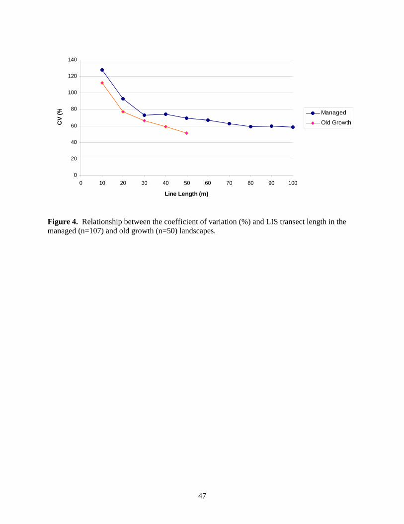
0

20

40

60

80

100

120

140

0 10 20 30 40 50 60 70 80 90 100

Line Length (m)

CV

(% Managed

Old Growth

Figure 4. Relationship between the coefficient of variation (%) and LIS transect length in the managed (n=107) and old growth (n=50) landscapes.

47

Alpha = 0.05, Power = 0.9 Alpha = 0.05, Power = 0.8

Req

uire

d S

ampl

e S

ize

Alpha = 0.10, Power = 0.8 Alpha = 0.10, Power = 0.9

True Change in Mean CWD Volume (m3/ ha) Figure 5. Minimum sample size required on average to detect a specified change in mean CWD volume (m3/ha) at a predefined alpha and power level using a specified LIS transect length in the managed landscape.

48

Alpha = 0.05, Power = 0.8 Alpha = 0.05, Power = 0.9

Req

uire

d S

ampl

e S

ize

Alpha = 0.10, Power = 0.8 Alpha = 0.10, Power = 0.9

True Change in Mean CWD Volume (m3/ ha) Figure 6. Minimum sample size required on average to detect a specified change in mean CWD volume (m3/ha) at a predefined alpha and power level using a specified LIS transect length in the old growth landscape.

49

0

20

40

60

80

100

120

140

Managed Old Growth

Vol

ume

(m3 /h

a)

Figure 7. Mean (+SE) coarse woody debris volume in the managed and the old growth landscapes.

50

0

10

20

30

40

50

60

70

8-20 cm 20-40cm 40-60cm >60cm

Old GrowthManaged

a)

Vol

ume

(m3 /h

a)

b) Size Class

0

0.1

0.2

0.3

0.4

0.5

0.6

0.7

8-20 cm 20-40cm 40-60cm >60cm

Old GrowthManaged

Pro

porti

on o

f Vol

ume

Size Class Figure 8. Mean (+SE) volume (a) and proportion of volume (b) of CWD across size classes by landscape.

51

0.00

0.05

0.10

0.15

0.20

0.25

0.30

0.35

0.40

0.45

0.50

1 2 3 4 5 6

Old GrowthManaged

Decay Class

Pro

porti

on o

f Vol

ume

Figure 9. Proportion of volume by decay class for the managed and old growth landscapes.

52