Retrospective Theses and Dissertations Iowa State University Capstones, Theses andDissertations

1986

Cost-benefit analysis in human resources activities:an examination of the robustness of the generalutility functionSue Margaret AndersonIowa State University

Follow this and additional works at: https://lib.dr.iastate.edu/rtd

Part of the Industrial and Organizational Psychology Commons

This Dissertation is brought to you for free and open access by the Iowa State University Capstones, Theses and Dissertations at Iowa State UniversityDigital Repository. It has been accepted for inclusion in Retrospective Theses and Dissertations by an authorized administrator of Iowa State UniversityDigital Repository. For more information, please contact digirep@iastate.edu.

Recommended CitationAnderson, Sue Margaret, "Cost-benefit analysis in human resources activities: an examination of the robustness of the general utilityfunction " (1986). Retrospective Theses and Dissertations. 8136.https://lib.dr.iastate.edu/rtd/8136

INFORMATION TO USERS

While the most advanced technology has been used to photograph and reproduce this manuscript, the quality of the reproduction is heavily dependent upon the quality of the material submitted. For example:

• Manuscript pages may have indistinct piint. In such cases, the best available copy has been filmed.

• Manuscripts may not always be complete. In such cases, a note will indicate that it is not possible to obtain missing pages.

• Copyrighted material may have been removed from the manuscript. In such cases, a note will indicate the deletion.

Oversize materials (e.g., maps, drawings, and charts) are photographed by sectioning the origin^, beginning at the upper left-hand comer and continuing from left to right in equal sections with small overlaps. Each oversize page is also filmed as one exposure and is available, for an additional charge, as a standard 35mm slide or as a 17"x 23" black and white photographic print.

Most photographs reproduce acceptably on positive microfiim or microfiche but lack the clarity on xerographic copies made from the microfilm. For an additional charge, 35mm slides of 6"x 9" black and white photographic prints are available for any photographs or illustrations that cannot be reproduced satisfactorily by xerography.

8703683

Anderson, Sue Margaret

COST-BENEFIT ANALYSIS IN HUMAN RESOURCES ACTIVITIES: AN EXAMINATION OF THE ROBUSTNESS OF THE GENERAL UTILITY FUNCTION

Iowa State University PH.D. 1986

University Microfilms

! ntsrn sti O n 8.! 300 N. Zeeb Road, Ann Arbor. Ml 48106

PLEASE NOTE:

In all cases this material has been filmed in the best possible way from the available copy. Problems encountered with this document have been identified here with a check mark V .

1. Glossy photographs or pages

2. Colored illustrations, paper or print

3. Photographs with dark background

4. Illustrations are poor copy

5. Pages with black marks, not original copy

6. Print shows through as there is text on both sides of page

7. Indistinct, broken or small print on several pages

8. Print exceeds margin requirements

9. Tightly bound copy with print lost in spine

10. Computer printout pages with indistinct print

11. Page(s) lacking when material received, and not available from school or author.

12. Page(s) seem to be missing in numbering only as text follows.

13. Two pages numbered . Text follows.

14. Curling and wrinkled pages

15. Dissertation contains pages with print at a slant, filmed as received

16. Other

University Microfilms

International

Cost-benefit analysis in human resources activities:

An examination of the robustness of the general utility function

by

Sue Margaret Anderson

A Dissertation Submitted to the

Graduate Faculty in Partial Fulfillment of the

Requirements for the Degree of

DOCTOR OF PHILOSOPHY

Major: Psychology

Approved :

In Charge of Major Work

ate College

lova State University

Ames, Iowa

1986

Signature was redacted for privacy.

Signature was redacted for privacy.

Signature was redacted for privacy.

ii

TABLE OF CONTENTS

INTRODUCTION

Statement of the Problem

LITERATURE REVIEW

Theoretical Models

Indices

Applications

METHOD

SD y

Wp

Full Model

RESULTS

SD y

4>/p

Combined Analyses

DISCUSSION

Statistical implications Substantive Implications

<p/p

Statistical implications Substantive implications

General Implications

Directions for Future Research

REFERENCES

iii

LIST OF TABLES

Page

Table 1. The effects of distributional truncation on percentage of employees eliminated, SD , and error ^ 50

Table 2. Comparison of percentages falling above lowest acceptable standardized score in normal versus reflected gamma 54

Table 3. Increase in marginal standardized job per­formance with a normal distribution of predictor performance and increasing truncation of job performance 58

Table 4. Increase in marginal standardized job performance with a reflected gamma distribution of predictor performance and increasing truncation of job performance 60

Table 5. Absolute marginal error in the use of the theoretical normal versus the reflected gamma distribution 62

iv

LIST OF FIGURES

Page

Figure 1. Effect on mean of job performance of moving performance from 15th to 85th percentile 10

Figure 2. Taylor-Russell model 13

Figure 3. Normal versus reflected gamma distributions of predictor performance 55

1

INTRODUCTION

Statement of the Problem

An important question in determining the usefulness of any per­

sonnel practice involves the expected costs and benefits of the practice

to the organization. Activities such as selection, training, and per­

formance appraisal may involve substantial expenditures of time and money;

yet, only rarely is the "bottom line" dollar benefit of a given program

considered at all.

Landy and Farr (1983) noted that personnel research often comes

under attack because of its seemingly superficial concern for cost-

effectiveness. According to Cascio (1980), human resources management

activities (i.e., those activities associated with the attraction, se­

lection, retention, development, and utilization of people in organiza­

tions) are generally evaluated in either behavioral terms (such as reac­

tion measures, learning tests, or observations of changes in employee be­

havior) or statistical terms (such as percentages, means, standard devia­

tions, or correlation coefficients). Landy, Farr, and Jacobs (1982)

noted that, for several decades, psychologists have faced the problem of

determining the usefulness of various strategies which are important in

the personnel process. Roche (in Cronbach & Gleser, 1965) mentioned that

the development of a meaningful criterion of an employee's performance is

probably the most important problem facing the personnel psychologist.

Traditionally, the method of choice has been to follow the path of

least resistance, and global measures such as supervisor ratings of

2

performance have been used to represent a complex, multi-faceted be­

havior. This often means that determination of whether or not organi­

zational goals are being met is difficult at best and sometimes im­

possible.

In attempts to document the efficacy of personnel procedures,

industrial psychologists have suggested a variety of criteria against

which their activities should be judged. These criteria include the

increase in the number of "successful" employees hired, the increase in

average level of performance among employees, or, more recently, the

amount of savings (through use of the program or activity) in terms of

dollars. Cascio (1980) pointed out that a reluctance to assess personnel

practices in monetary terms has persisted, although he also noted that

several different methods for cost-benefit analyses have been available

for many years. The reluctance seems to stem from the long-standing

belief that human resource functions are somehow "different" from all

other organizational activities and, as such, are not amenable to inter­

pretation in the context of dollars.

An area which as traditionally been accorded a great deal of concern

in the context of human resources activities is selection. Effective

selection (that is, choosing the most appropriate candidates in a fair

and cost-efficient manner) is obviously of critical importance in the at­

tainment of organizational goals. The actual monetary value of (more)

effective selection, however, is rarely, if ever, addressed.

An almost universally used personnel practice is performance ap­

3

praisal, which refers, simply, to the evaluation of employee performance,

either for administrative purposes (such as compensation) or for direc­

tive purposes (such as training). Although widely used (indeed, it is

difficult to imagine an organization where employee performance is not

appraised), it is difficult to find instances where the cost of per­

formance appraisal versus the potential benefits of such appraisal is

systematically assessed. This makes it difficult to determine if one

approach to performance appraisal might be preferable to another in terms

of attainment of various organizational objectives.

Another important illustration of the inadequacy of traditional

approaches to evaluating personnel practices concerns training, also re­

ferred to as "human resources development." Industrial training is de­

fined by Goldstein (1980) as the acquisition of skills, concepts, or

attitudes intended to result in improved performance in an on-the-job

environment. The goal or purpose of training may vary from personal growth

to improved organizational efficiency; however, typically the only type of

evaluation involves assessing employee reactions to the training. While

such reactions are obviously important in the assessment of face validity

(i.e., the extent to which trainees feel the training is appropriate),

they are woefully inadequate in determining the "bottom-line" benefit of

training to the organization. Given the fact that organizations in the

United States spend upwards of several billion dollars annually on train­

ing (Wexley & Latham, 1981), the over-emphasis on trainee reactions as the

sole measure of efficacy of training is particularly suspect.

4

According to Goldstein (1980), in the most primitive kind of evalu­

ation, appropriate measurement methodology is ignored and decisions are

based upon anecdotal trainee (and sometimes trainer) reactions. Most

analysts realize the limits of this approach; however, this is still the

"typical" (i.e., most common) approach. At the other end of the rigor

continuum is the kind of approach which may be just as unproductive in

terms of providing usable information. This approach is based on strict

adherence to the basic experimental methodologies of academic labora­

tories. Frequently, such designs are completely inappropriate in terms

of the limitations of the organizational environment; as such, they are

often abandoned in frustration before any conclusions are reached. The

most appropriate strategy would thus be one which strove for a balance

between unstructured and over-structured — i.e., one that could provide

both the researcher and the personnel practitioner with usable, easily

interpretable information. A consideration which may further complicate

the evaluation of the efficacy of training concerns distributional as­

sumptions. Little attention is given to assessing the distribution of

performance before training; even less is given to assessing whether the

training itself affects the shape of the performance distribution. In­

deed, it might reasonably be argued that the major goal of training is

to shift the performance distribution in such a way that it becomes nega­

tively skewed.

Note that nearly all approaches to evaluating human resources ac­

tivities have one of two major limitations: Either they are inadequate

5

to determine if the activity is really effective (and, if so, effective

in what sense) or they require more employees/subjects than are typical­

ly available. Only occasionally are such activities subject to any sort

of cost-benefit analyses. In the rare instances where attention is

given to determining the cost-benefit ratio of a particular personnel

function, no attempts are made to determine if the underlying assump­

tions on which the interpretability of such analyses rests are met.

A simple summarization of the inadequacy of traditional approaches

to evaluating the organizational effectiveness of various human resources

activities was provided by Brodgen (1950), who noted that "the general

objective of firms is to make money. This is not indicative of a ma­

terialistic attitude; it is simply the truth. No company can stay in

business without at least breaking even." It is thus cogent to ask how

any personnel practice affects an organization's ability to do so. In

terms of many personnel functions, such as selection, training, and per­

formance appraisal, no typically used measure will allow an assessment

of this criterion.

Landy and Farr (1983) observed that, despite the fact that various

approaches to cost-benefit analysis in a variety of h'jman resources func­

tions have been available for many years, few attempts to systematically

document cost-benefit concerns can be found. This, they contend, is most

probably due to two major reasons:

(1) Until recently, most applications of cost-benefit concerns involved testing. Since testing has, from time to time, come under attack from a fair employment view, it is under­standable that procedures correlative to testing have also been ignored.

6

(2) Many procedures central to cost-benefit analyses have not been subject to rigorous theoretical examination.

As such, it is understandable that a reluctance to employ such analyses continues.

In light of the above considerations, this study has several major

purposes: First, the historical development of various approaches to

evaluating the effectiveness of personnel practices, in general, and of

different kinds of personnel programs, in particular, will be described

in detail, along with the important limitations (both theoretical and

practical) of these different approaches. One potentially viable ap­

proach to addressing the need for accountability in human resources func­

tions relies on utility analysis, which refers to an estimate of benefits

expected to result from a particular decision. Several researchers (i.e.,

Schmidt, Hunter, McKenzie, & Muldrow, 1979; Schmidt, Hunter, & Pearlman,

1982) have suggested that utility analysis is appropriate for cost-benefit

studies of personnel functions. Specifically, they contend that parame­

ters of organizational settings are similar enough to the theoretical as­

sumptions of utility theory to warrant application of the theory.

Boudreau (1983b) noted that, although mathematical equations for

expressing the utility of selection devices in monetary terms have been

available for more than 30 years, such equations have not been widely

used. He contended that this failure to employ them may be due to sever­

al reasons, such as misconceptions regarding the necessary statistical

relationships, the assumption that costly validity studies are necessary

in every situation, and the difficulty of accurately estimating the vari­

7

ability of job performance in dollars.

Though actual use of utility theory to determine potential mone­

tary benefits is apparently not widespread (Landy & Farr, 1983), an

important preliminary step in the demand for accountability involves

the determination of robustness. No studies to date have rigorously

investigated the sensitivity of the utility function to violations of

its underlying assumptions. Because "real-life" data (i.e., that which

are 'collected in an actual organization) may differ substantially from

theoretical expectations, it is critical to determine if departures from

such assumptions affects the viability of the function's use. As such,

the major purpose of this study is to examine the robustness of the

utility function. Such variables as the number of employees involved

(i.e., the number tested or trained) and the cost of the activity are

relatively straightforward and, hence, are not subject to a great deal

of misinterpretation. Other variables, however, such as the distribu­

tions of predictor performance, job performance, etc., may be consider­

ably less straightforward and thus need tc be rigorously examined, in the

context of their potential impact on organizational decision-making.

In the context of this study, the term utility will be used to

refer to the expected benefits assumed to result from a particular

organizational decision or course of action. Robustness will, of

course, refer to the sensitivity of the utility model (as it may be ap­

plied to various personnel functions) to departures from underlying

theoretical assumptions. It is expected that an examination of the

8

robustness will help assess the feasibility of using the function in an

applied setting and is thus an important first step on the road to ac­

countability in human resources activities.

9

LITERATURE REVIEW

In order to illustrate some of the limitations of traditional meth­

ods of assessing the usefulness of personnel practices, as well as demon­

strate the applicability of utility analysis, some review is necessary.

More attention has been given to selection than any other specific aspect

of the personnel process; thus, any review must necessarily emphasize an

analysis of selection, followed by attempts to extend the logic to other

personnel functions.

Theoretical Models

Munsterberg (1914) had first noted the importance of differential

placement into jobs according to aptitudes; he pointed out the now-obvious

fact that people differ in terms of abilities and are thus differentially

suited for placement into different types of jobs.

Hull (1928) enlarged upon Munsterberg's notions in an early approach

tc the quantification of work performance (a necessary first step in the

assessment of monetary gain or loss). Hull conceived of using the ratio

of best-to-poorest worker as a means of targeting individual differences

in work performance. Though simple, Hull's approach has some intuitive

appeal. He implied that utility might be gained by moving the mean of

the performance distribution up towards the high end of the performance

scale; this is graphically illustrated in Figure 1, where, obviously,

the overall performance of the workgroup as a whole can be improved by

attention to those workers who are on the low end of the performance dis-

10

-X '40J0

X X X X X X X X

X X

-X»425

X

X

X ' ^

X X

X X X X X X X

X X X X X X

X X X X X X X X

X X X X X X X X

X x x x x x x x x x

X x x x x x x x x x

X X x x x x x x x x x x

X X x x x x x x x x x x I I

0 S10 1S 202SX3S40 46 50 S5 60 65 70 75 0 S 10 1S 20 3SX3S 40 4S50S5SOG57075

Figure 1. Effect of performance improvement on group mean

tribution (relatively).

Tnis could be accomplished by substituting more competent workers

for their less competent colleagues, either through more precise initial

selection procedures or through on-the-job training procedures. Hull was

basically enlarging upon Munsterberg's ideas by noting that periormance

variation could occur within, as well as across, particular jobs. Note

that even at this early stage, it was recognized that the usefulness of

the best-to-poorest worker ratio would depend at least partially on

the nature of the job in question. In some types of jobs, lictle per­

formance variation occurs. For example, the ratio of best-co-pooresc

worker may be as low as 1:1.4 for heel trimmers and as high as 1:5.1 for

spoon polishers (Hull, 1928).

A potential problem with Hull's model concerns the assumption of a

s^rmnecrical distribution of performance. It is doubtful that such sym­

11

metry would be found often in practice, as extremely poor workers enjoy

little, if any, job tenure; thus, their low performance scores would tend

to drop out of the distribution of performance scores. While in theory

this would simply narrow the range of performance scores, in actual prac­

tice it may prove difficult to interpret the resulting ratio. For ex­

ample, the "poorest" worker (relatively speaking) may still be one whose

performance is adequate. A related problem involves the difficulty of

quantifying output in some types of jobs. Many jobs (such as manager,

engineer, police officer, to name several) simply do not lend themselves

to easy quantification of output.

Indices

The validity coefficient, the most common means for assessing the

efficacy of a particular selection method, is usually defined as the

correlation of test score with outcome or criterion score. (Note that

in this context, the term "test" may refer to any selection device, in­

cluding, for example, paper-and-pencil tests, interviews, letters of

recommendation, etc.)

A nuEber of different approaches to interpreting the validity co­

efficient have been proposed. All are relatively simple functions of ̂

which bear directly upon an evaluation of the extent to which one vari­

able may be predicted from the other when the correlation coefficient

is of a given magnitude. Eistorically, the oldest approach is the

index of forecasting efficiency, where ̂ = 1 - /I - r^. This index

12

compares the standard error of scores predicted by means of the test

to the standard error of scores when there is no information on the in­

dividual and the group mean must be used as an estimator of the indi­

vidual's score. The proportionate reduction of the standard error is

taken as a measure of the value of the test.

A modification of this is called the coefficient of alienation, k,

where k = /(I - r^) (Kelley, 1923). Taylor and Russell (1939) de­

scribed where ̂ = /k/2. Another approach uses , the coefficient

of determination, as a means of assessing the value of the selection

device. This expression is intended to illustrate the value of the se­

lection device by expressing the ratio of predicted (or "explained")

variance to total variance. Logically, the more variance in job per­

formance that can be explained, the more valuable the test for selection.

Taylor and Russell (1939) also recognized the importance of indi­

vidual differences and added the concepts of validity, selection ratio

(proportion of candidates who are actually selected), and base rate (pro­

portion of present employees who are considered successful). They noted

that traditional approaches to evaluating the correlation coefficient as

the appropriate measure of selective efficiency have one important draw­

back in common. As the size of the correlation coefficient increases,

the extent to which one variable can be predicted from the other in­

creases more rapidly. They contended that widespread acceptance of such

measures as the correct way of evaluating correlations led to consider­

able pessimism with regard to the magnitudes of correlations usually ob—

13

cained in employment settings. Their model was intended to demonstrate

that when the tests are used for selection, correlations within the

range of .20 to .50 (the magnitudes which are most frequently found in

employment settings) may represent considerably more than 2% to 13% of

the effectiveness of a correlation of unity.

Such concepts underscore the fact that the value of a given test

for selection varies as a function of the parameters of the situation in

which it is used. The Taylor-Russell model assumed normality of both

predictor and underlying criterion variables, linearity of the regres­

sion of the criterion on the predictor, and a validity coefficient in the

form of a Pearson product-moment correlation. Their model can be graph­

ically depicted as follows:

predictor

criterion cut-off

reject accept

In this schema, A represents employees who met or exceeded the predictor

cut-off and later proved to be successful in terms of job performance.

14

B represents employees who met or exceeded the predictor cut—off but

whose job performance was unsatisfactory. C represents those who were

rejected (or the basis of predictor performance) and would have been

unsatisfactory employees had they been hired. D represents candidates

who were rejected but who would have been successful had they been

hired. (Note that C and D are hypothesized groups, as candidates who

were rejected on the basis of their predictor performance could obvious­

ly not be evaluated on later job performance.)

Taylor and Russell also constructed a set of tables which demon­

strated that even a selection device with seemingly low validity (i.e.,

a modest test-criterion correlation) can substantially increase the pro­

portion of selectees who will be successful (although this expected in­

crease is largely a function of the proportion of current employees who

are considered successful).

A major problem with the Taylor-Russell model concerns the neces­

sity of arbitrarily dividing employees into only two groups: successful

and unsuccessful. It is unlikely that an employee who barely meets a

min-i-muTn standard for qualifying as "successful" is as valuable to the

organx^aCioii as one who ils substantially above the cut-off - (A related

problem concerns the decision of where to draw the line separating suc­

cessful from unsuccessful employees. Such a decision is generally some­

what arbitrary and, as such, is highly vulnerable to the imposition of

values.) Another potential problem was noted by Smith (1948) who pointed

out that the Taylor-Russell tables, as ordinarily used, tend to over­

15

estimate prospective gains in effectiveness because of their failure to

allow for known pre-existing validities and selection ratios. The ta­

bles assume that the applicant group and the present employee group are

similar; this is equivalent to assuming that 100% of all applicants

are being hired and retained, that current selection procedures have

zero validity, or that both conditions exist. Such assumptions are un­

realistic, as it is very likely that the present selection ratio is less

than 1.0 and the validity of^present selection procedures (unless ran­

dom selection is in use) is greater than 0.0. Obviously, these consider­

ations limits the effective use of the model in most organizational set­

tings .

As early as 1946, Brogden formally demonstrated that is not ap­

propriate for interpreting the validity coefficient in the context of a

selection decision. He emphasized the notion of evaluating decisions

directly on a utility scale to interpret the validity coefficient; he

concluded that the gain from use of a test in selection is linearly

related to the validity of the test. Brogden showed that a test's

validity is a linear function of the difference between the mean for

the "successful" group and the mean for the population. Also, he

showed that ^ equals the proportion improvement over chance that %s

possible with different selection ratios. Brogden's approach helped

illustrate a major weakness of both E and r_ (and modifications there­

of, as noted above). Both may give an overly pessimistic view of the

"real" value of a given test for selection. If r_ = .50, for example.

16

^ describes the test as predicting only 13% better than chance, while

2^ describes the same test as accounting for 25% of the variance. An­

other potential weakness involves the lack of intuitive meaning of

either term. To describe a particular test as explaining 25% of the

variance in job performance is somewhat imprecise in terms of predict­

ing what benefits may accure to the organization through use of the

test. Likewise, describing the same test as reducing the standard er­

ror by 13% is equally imprecise in an applied sense, as well as intui­

tively meaningless to the typical personnel practitioner. Such a de­

scription obviously does not provide any idea of the true practical value

of the test to the organization.

The model proposed by Brogden and Taylor (1950) emphasized the im­

portance of a dollar unit as the most desirable criterion of industrial

efficiency. Their model was based on Brogden's earlier formulations and

assumed identical (but not necessarily normal) and continuous distribu­

tions for predictor and criterion, as well as linearity of the regres­

sion of the criterion on the predictor and a constant selection ratio.

Brogden (1946) had shown that when these assumptions are met, the validi­

ty coefficient itself is a direct index of selective efficiency. If cri­

terion performance is expressed in standard score units, then over all

individuals r^ represents the ratio of the average criterion score made

by persons selected on the basis of their predictor scores (Zz^).

The model involved rescaling such factors as production, errors,

accidents, etc., into a standard dollar metric. Such rescaling, when

17

applied to the assessment of work performance, allowed an estimate of

an individual's contribution to the organization. Brogden and Taylor

also proposed extending such logic to training costs, turnover, and on-

the-job productivity to show the potential value of an applicant or

employee. In using their cost accounting procedures to develop a dol­

lar criterion, a number of elements must be considered. Brogden and

Taylor listed the following as examples:

1. average value in dollars of production or service units

2. quality of objects produced or services performed

3. overhead

4. errors, accidents, etc.

5. where applicable, public relations factors

6. cost of time of other personnel consumed

Although theoretically sound, their model is still plagued by the un-

tenability of the assumption that performance is identically distributed.

A more practical drawback concerns the extensive investment in cost-

accounting procedures necessary to use the model appropriately. A sub­

stantial investment in time and money is required to accurately assess

all relevant costs. This may make potential benefits less than antici­

pated (i.e., the cost of determining costs and benefits may be sub­

stantially greater than potential benefits).

The Naylor-Shine model (1965) assumed a linear relationship between

validity and utility which holds true at all selection ratios. Unlike the

Taylor-Russell model, however, their model does not require arbitrary

18

dichotomization of employees into satisfactory-unsatisfactory groups.

Naylor and Shine also constructed a set of tables which can help deter­

mine mean increase in average standardized criterion score for the se­

lected group over that observed for the total group. Note, however,

that while this is somewhat interpretable in terms of performance expec­

tations, it still does not describe the value to the organization of us­

ing that test; nor does their model easily lend itself to personnel

functions other than selection.

Cronbach and Gleser (1965) proposed a modification of the Brogden-

Taylor model. Customarily, they noted, the value of a test is inter­

preted in terms of improvement over chance. They suggested that expected

outcome under any strategy should be evaluated on an absolute utility

scale. The value of a strategy which employs a test should be compared

to the utility from the best "a priori" strategy — that is, the best

strategy not using the test. The difference between the two is the gain

from testing and is positive or negative depending on the cost of the

test. (This implies that an extremely expensive test, even one which

is highly accurate in terms of prediction, may be more detrimental than

helpful, because the added cost of using it more than negates added bene­

fits. Thus, although precision may be great, the cost of precision may

be too high.)

The Cronbach-Gleser model is based on the general utility equation

from decision theory. This general equation makes no distributional as­

sumptions about the variables involved (although certain equations de-

19

rived from it for specific situations do). Accordingly, the equation

is:

U = NZp? ZPc/Yt ®c - KZPyCy

where

U = utility of the set of decisions

N = number of persons about whom decisions are made

Y = information category

t = treatment

c = outcome

e =value of outcome c

= cost of gathering information

A drawback to convenient use of this equation is its inapplicability for

yielding results interpretable with respect to industrial decisions.

Accordingly, the equation was modified to make it more tenable for dif­

ferent types of selection.

Cronbach and Gleser described two major types of selection decisions

fixed treatment, where individuals are chosen for one specific treatment

which cannot be modified, and adaptive treatment, in which the decision

maker is allowed to adjust the treatment according to the quality of in­

dividuals chosen. Also, decisions may involve quotas (where a fixed num­

ber of individuals must be selected), or flexible quotas, where the de­

cision maker has the option of accepting as few or as many individuals as

desired, depending on the qualifications of the candidate pool.

20

In fixed treatment selection, the basic goal of the decision maker

is to accept those individuals whose expected pay-off is highest, within

the constraints of what information is available and what quota may have

to be filled. As such, the net gain in utility per man tested from se­

lection for a fixed treatment is linearly related to the value of the

test:

U = r SD Z ye e y

This equation is based on the following assumptions :

1. Decisions are made regarding an indefinitely large population of persons. This "a priori" population consists of all applicants after screening by any procedure now in use that will continue to be used.

2. Regarding any person there are two possible decisions: Accept or reject.

3. Each person has a test score y. with mean = 0 and standard deviation = 1.

4. For every person, there is a payoff which results when the person is accepted. This payoff has a linear regres­sion on test score. The test will be scored so that r^ is positive.

5. T^hen a person is rejected, the payoff e^g results. This payoff is unrelated to test score, and may be set equal to zero.

6. The average cost of testing a person on test y is C^, where is greater than zero.

7. The strategy will be to accept high scoring individuals in preference to others. A cutoff of y will be located on the y continuum so that any desired proportion (p') of the group falls above y'. Above that point, proba­bility of acceptance is 1.00; below it, 0.00.

21

Cronbach and Gleser also developed equations appropriate for fixed

treatments with variable quotas and for adaptive trestments with both

fixed and variable quotas.

This model re-emphasized the importance of cost, as they noted

that any selection procedure should be assessed in terms of its incre­

mental contribution relative to the best strategy available using prior

information. If, as Brogden (1950) had pointed out, the criterion

can be expressed in cost-accounting terms as an estimate of the dollar

savings obtained by selecting a given individual instead of an average

applicant and r^ gives the percentage of possible savings, then the

product (r )(& ) [where O is criterion standard deviation in dollars] -xy y y

estimates the increase in saving per unit increase in standard score.

Thus, any new procedures must represent an improvement over current

practices. Cronbach and Gleser also pointed out that the cost of a se­

lection procedure is of great importance, as even a "perfect" means of

selection (i.e., where a correlation of 1.0 between predictor and cri­

terion exists) could be of little or no value if the costs associated

with using it are too great. Note that this is an important consider­

ation in the use of any personnel procedure. A seemingly effective train­

ing program (i.e., one which substantially improves work performance over

base rate), may cost more than the gain in performance is worth to the

organization. In such a case, the logic of describing such a training

program as effective is obviously suspect. This underscores the need for

a means of objectively quantifying in monetary terms the cost-benefit

22

ratio of any personnel practice, including selection, training, per­

formance appraisal, etc.

Applications

Roche (in Cronbach & Gleser, 1965) described the application of

the Brogden-Cronbach-Gleser model to an industrial setting. To arrive

at a reasonable estimate of the profit which accrues to the organization

as a result of an employee's work, the cost accounting methods developed

by the company (a manufacturer of heavy equipment) were used. Basically,

the method is one of standard costing, a commonly-used technique in

volume production accounting. Standard cost for the company's products

was determined fay obtaining cost data on three basic factors: material

used in production, direct labor hours used to operate on materials, and

facility usage required to perform direct labor. The payoff for each

individual depended on a productivity measure called the performance ra­

tio. For each machining operation, the Time Study Division of the organ­

ization had established a time standard. The length of time required for

a competent operator to complete the machining operation was established

by standard time study procedures; thus, the number of parts per hour that

an operator should be able to process was known. An operator's performance

ratio for any period of work was then computed by dividing actual produc­

tion by standard hourly production. Each operator's payoff was determined

by computing a typical performance ratio (mean performance over the six-

month duration of the study), adjusting this performance ratio for below

standard production, and computing average profit of adjusted typical per­

23

formance ratio with data provided by the company's Cost Analysis Divi­

sion. The cost of testing involved only the actual costs of the tests

themselves. Roche concluded that the results of his study demonstrated

that a dollar criterion could be developed (albeit with some expense

and effort incurred) for a typical fixed treatment employee selection

procedure.

Curtis and Alf (1969) examined the functional relationship between

three indices of predictive efficiency: r^, , and and three measures

of practical significance: increase in criterion mean, expected propor­

tion judged "satisfactory," and expected proportion in 10 criterion cate­

gories. Overall, r^ was judged to be the best measure in terms of a linear

relationship with the measures of practical significance. Both and

according to Curtis and Alf, may lead to unrealistically pessimistic eval­

uations of the potential value of the test.

Sands (1973) proposed a model called CAPER (Cost of Attaining Per­

sonnel Requirements) which helped to determine an optimal recruiting-

selection strategy. Specifically, the CAPER model provided the personnel

manager with all the information necessary to minimize the expected costs

of selecting, inducting, and training a sufficient number of persons to

meet some specific quota of satisfactory personnel. Sands noted that the

CAPER model had several important advantages over more traditional ap­

proaches. First, it allowed communication of easily-interpretable re­

sults — specifically, results which were stated in terms of dollars.

Also, it recognized the fact that the selection procedure has important

24

implications for the entire personnel system. In contrast to a tra­

ditional correlational model (i.e., one where the sole means for evalu­

ating the efficacy of a particular means of selection is the magnitude

of the correlation coefficient), the CAPER model takes into account the

utility or cost of various decision-outcome combinations, including cor­

rect selection and rejection and erroneous selection and rejection.

In order to effectively use the CAPER model, as it is described by

Sands, the following information is required: the quota, the base rate,

and the proportion of previous successes and failures. Also, the fol­

lowing cost data per person must be specified: recruiting, selection,

training, erroneous acceptance, and erroneous rejection. Such informa­

tion is, according to Sands, usually readily available; thus, the imple­

mentation of the model is fairly easy and well worth the time and/or

money investment required. (Note, however, that at least some arbitrary

value judgments are required. For example, how should the cost of er­

roneous rejection be determined? Obviously, this value may be determined

differently by different people.)

Schmidt and Hoffman (1973) compared actual savings resulting from

the use of a selection device to savings predicted from (a) the Taylor-

Russell interpretation, (b) Brogden's interpretation, and (c) the general

utility equation of decision theory. The utility analysis was applied

to a weighted application blank developed to predict turnover among

nurse's aides. They concluded that the most accurate estimate was ob­

tained with the general decision theory equation using empirical (rather

25

than theoretical) probabilities.

Lee and Booth (1974) performed an analysis to assess the poten­

tial monetary value of using a cross-validated weighted utility blank

for selection. They pointed out that a cost-benefit analysis was con­

sidered a necessary step in terms of justification of the use of the

blank. By means of a questionnaire distributed to supervisors of cler­

ical employees, they determined the average time spent in supervision

of new employees for progressive one-month periods after initial hire.

From this and other values, four costs associated with turnover were de­

rived; cost of recruiting, cost of supervisory training, cost of loss

of employee productivity during training period, and cost of fringe bene­

fits during training period. Their analysis also employed the selection

rate and base rate as variables. They estimated maximum savings in se­

lection to be approximately $250,000. Though they pointed out that var­

iations in supply and demand may affect the amount of savings, they also

contended that the utility estimates of the weighted application blank

are large enough to be significant from a practical point of view —

large enough, in fact, to warrant utility analysis of other approaches

to selection in order to accurately assess the practical benefit of

various selection strategies.

Cascio and Sibley (1979) evaluated the utility of the assessment

center as a selection device by means of the Brogden-Cronbach-Gleser

continuous variable utility model. They first noted that, although the

assessment center approach has received much kudos from a traditional

26

psychometric point of view, it has also been legitimately criticized for

ignoring certain external parameters of the situation that may largely

determine the overall value of utility of a selection device. Six such

parameters were identified and systematically varied: validity and cost

of the assessment center, validity of the alternative selection proce­

dure (i.e., the "a priori" strategy), selection ratio, standard devia­

tion of criterion (in other words, performance) in dollars, and number

of employees assessed. They concluded that, given the appropriate set

of parameters, significant savings in dollars could be realized through

use of the assessment center and, as such, use of the assessment center

approach as a selection device would be appropriate.

Perhaps, the most important contribution to the use of utility theory

in the context of selection decisions involved the 1979 study by Schmidt,

Hunter, McKenzie, and Muldrow. Their analysis examined the potential

savings which could accrue to the federal government through use of se­

lection devices with different levels of validity. They first noted that

the coefficient of determination continues to be used as a measure of the

efficacy of a selection device, although its use may reflect an under­

estimate of the true value of a valid selection test. This is a function

of the fact that the magnitudes of validity coefficients typically ob­

served in industrial settings make most tests appear to be only moderate­

ly predictive of future performance. Analogously, assessing the value of

a training program by simply asking employees their reactions is not suf­

ficient to determine what, if any, tangible benefits may accrue to the

27

organization through the use of that training method.

As an alternative, Schmidt et al. proposed using the term "utility"

to describe an analysis of the potential benefits associated with the use

of a given selection device. Berkson (1947) had originally defined util­

ity as the proportion of unsuccessful candidates eliminated and cost as

the proportion of successful applicants rejected. Blum and Naylor (1968)

defined the utility of a particular selection device as the degree to

which use of that selection device serves to improve the quality of those

selected beyond what would have occurred had that selection device not

been used. Quality may be defined in several different ways as (1) the

proportion of individuals in the selected group who are considered suc­

cessful, (2) the average standard score on criterion for the selected

group, or (3) the dollar payoff to the organization resulting from the

use of a particular selection device. Note that it is relatively simple

to extend this logic to describe the utility of other personnel functions,

such as training: The utility of a training program is the degree to

which its use improves the quality of those trained beyond what would

have occurred had no such training been used.

Cronbach and Gleser (1965) provided perhaps the most useful defini­

tion. They described utility analysis as the determination of institu­

tional gain or loss expected to result from various courses of action

(outcomes). This general definition is easily applicable to other per­

sonnel functions: For example, what degree of objectives (i.e., monetary)

gain or loss can be expected to result from different kinds of training

28

decisions? Likewise, what degree of monetary gain might be realized

from the implementation of a more effective performance appraisal sys­

tem? Such a question might reasonably be asked of virtually any kind

of human resource activity, including recruiting, selection, placement,

training, performance appraisal, promotion, layoff, discharge, etc.

Given the above considerations, the equation Schmidt et al. em­

ployed as most appropriate in terms of organizational decision making

was

AU = t N(r^ - r^)SD^ (jj/p - N(C^ - C^)/?

where

AU = expected change in utility

t = average tenure of individual in the organization

N = number of persons tested

r^ = validity of proposed selection procedure

r^ = validity of current selection procedure

SD^ = standard deviation of performance expressed in dollars

<j) = ordinate of normal curve expressed at point p

p = selection ratio

= cost of proposed procedure

= cost of current selection procedure

They concluded that the computation of SD^, the standard deviation

of performance in dollars, has typically been the Achilles' heel of de­

cision-theoretic attempts to assess the utility of a selection device.

Their approach involved using a questionnaire-type instrument to ask

29

supervisors of computer programmers about their estimates of the value

of poor, average, and good programmers. (Supervisors were instructed

to consider the cost of hiring programmers from outside the government.)

Again, however, the determination of SD^ rested on the tentative assump­

tion that performance is normally distributed. [Note that Tiffin and

Vincent (1960) investigated the problem of empirical versus hypothetical

distributions with respect to the Taylor-Russell tables; they concluded

that the two distributions matched quite well and use of hypothetical

distributions is generally appropriate in most research situations. No

other attempts to document the match of theoretical versus empirical dis­

tributions of the various cost-benefit approaches exist.] Accordingly,

in a later reformulation, Schmidt, Hunter, and Pearlman (1982) simplified

this admittedly somewhat time—consuming procedure by contending that SD^

is equal to approximately 40% of annual salary. Schmidt et al. (1979)

determined that the annual savings that could be realized ranged from

several million dollars to well over a billion dollars.

Another attempt to apply this approach involved a study by Schmidt,

Hunter, and Pearlman (1982). They contended that the model could also

be applied to the training function, and, as such, they reformulated the

equation as follows:

AU = T N SD d - NC y

where

AU = the dollar value of the training program

T = the number of years duration of the training effect

on performance

30

N = the number of persons trained

d = the true difference in job performance between the average trained and untrained employee in SD units

SD = the standard deviation of job performance in dollars ^ of the untrained group

C = the cost of training per trainee

Actual computations involved using hypothetical values of T, N, SD^, d,

and C, rather than actual data; thus, their results should be considered

illustrative rather than conclusive. They contended, however, that the

dollar value of at least some interventions designed to improve employee

performance may be more significant than usually assumed. Perhaps, more

importantly, they concluded that the linear regression-based decision-

theoretic equations previously used to assess the impact in dollars of

valid selection procedures on workforce productivity can be adapted to

the evaluation of employee intervention (in other words, training) pro­

grams.

An obvious weakness of Schmidt et al.'s (1982) conclusion concerns

their use of hypothetical, rather than actual, data. Although their

conclusions are at least minimally encouraging (particularly from the

point of view of the trainer, who may be especially interested in a

dollar estimate of the effectiveness of training), their approach pro­

vides a model for potential application, rather than an empirical demon­

stration of actual savings. A potentially more serious criticism con­

cerns the lack of attention given to the distributions of performance

before and after training. Even if it is reasonable to assume that per­

31

formance is normally distributed before training, it can also be reason­

ably argued that the major purpose of training is to shift the distribu­

tion of performance from normal to somewhat negatively skewed (i.e.,

fewer "poor" performers and more "good" performers).

Landy and Farr (1983) described an attempt to apply the Schmidt et

al. utility model to the performance appraisal function. Specifically,

they wished to estimate the dollar value of the feedback component of

effective performance appraisal. Accordingly, they used the following

equation:

AU = t N d SDy - N(C^ - C^)

where

ATJ = expected increase in utility

N = 500

d = .60 (as estimated from a literature review)

SD = $20,000 (using the approach suggested by Schmidt et ^ al.)

C = $700 per employee (as calculated from the costs of developing the program, the time requir-d for the training of evaluators, and the time required for supervisors to carry out and feed back the results of the evaluation, as well as the "down time" of the manager being evaluated)

= $00 (there had been no prior procedure; hence, there was no prior cost)

Given these parameters, they concluded that the utility of introducing

a performance evaluation and feedback system would be approximately 5.3

million dollars for one year. A major flaw in their approach concerns

32

the computation of SD^. No specific information was addressed to the

concern of whether performance of managers is really normally distributed,

either before or after the training intervention (a major assumption of

the Schmidt et al. model). As such, their conclusions (while certainly

positive) are somewhat suspect in terms of the tenability of the under­

lying assumptions.

Despite Schmidt et al.'s contention that all personnel programs are

amenable to utility analysis, little, if any, effort to systematically

estimate the value of training in dollars has been undertaken. Ford

(1984) in a fairly typical study of the efficacy of training programs,

conducted an analysis to determine the benefits of using a Personalized

System of Instruction (PSI) to a large personnel training system. A

quasi-experimental randomized design was employed to compare a PSI ap­

proach to health care training with traditional techniques. "Effective­

ness" was determined by examining performance means in training modules

and performance appraisal data after 90 days on the job. "Efficiency"

was measured by recording the number of hours each trainee spent in

training, as it was assumed that the less time spent in training, the

greater the efficiency of that training. Costs were assessed by evalu­

ating the cost of the PSI purchase and upkeep against the cost of tra­

ditional training. Ford concluded that the PSI approach was far superior

in terms of both better performance and lower cost. Note that Ford did

not address the issue of translating performance into any dollar criteria.

For example, he did not consider potential savings to the organization

33

that could result through implementation of PSI as the primary method of

training. While his results are encouraging and certainly point to the

implmentation of PSI as the training method of choice, they are obviously

inadequate in evaluating how lauch benefit in dollars could be realized

through PSI.

Burke and Day (1986) conducted a meta-analysis of available studies

on managerial training in an effort to determine the extent to which

such training, which they term "pervasive," is effective. They concluded

that managerial training is, on the average, moderately effective. How­

ever, despite their contention that managerial training programs are quite

widespread, they were able to locate only 70 studies that included one or

more control groups. Perhaps, more importantly, their definition of "ef­

fectiveness" is largely bound by the criteria of effectiveness used in the

different studies. The large majority of studies included (23) involved

performance ratings as criteria; such ratings would fall into subjective

evaluations of bheavior as described by Kirkpatrick (1976). Only three

studies employed such objective measures as decrease in error rates as

criteria; none examined the cost-benefit ratio of managerial training.

While Ford's research (and that of others who have examined various

aspects of the personnel process in terms of their usefulness) is cer­

tainly laudable, it is at best only an imprecise representation of the

real extent to which an organization might benefit from an effective and

viable training program. It was noted above that traditional approaches

to evaluating the efficacy of different types of selection instruments

34

generally tend to underestimate the true value of such instruments.

Logically, the same might be said for other personnel functions. For

example, it is reasonable to argue that the real value of training to

an organization (that is, the value of the training in dollars) is sub­

stantially greater than usually assumed. The same argument might be

made for other human resources functions. As such, it is cogent to ask

if cost-benefit analyses based on the logic and assumptions of utility

theory (as developed by Cronbach & Gleser, 1965) could reasonably be

applied to the gamut of personnel functions. Before calling for whole­

sale application of the model, however, it is important to recognize that

frequently there may be a discrepancy between the assumptions of the model

and the nature of "real-life" data findings. As such, a necessary step

Involves a study of the robustness of the model — the extent to which

it is relatively insensitive to violation of its underlying assumptions.

This is critical in the applicability of the model, as frequently the

underlying assumptions may not be met in actual practice; thus, it is im­

portant to determine how various departures from the model's assumptions

affect the viability of the model as a solution to the problem of ac­

countability in the human resource function.

A potential problem pointed out by several researchers (Bobko, Karren,

& Parkington, 1983; Weekley, Frank, O'Connor, & Peters, 1985) centers on

the question of the true distribution of performance. The Schmidt et al.

(1979) technique is based on the rationale that if job performance (the

criterion) is normally distributed, then the difference between the values

35

of the products and services produced by the average employee (i.e.,

one at the 50th percentile) and those produced by an employee at the 85th

percentile in performance should be equal to the standard deviation of

the criterion.

In Schmidt et al.'s original study, they determined that estimates

of the difference between the 15th and 50th percentiles were "sufficient­

ly" equivalent to estimates of the difference between the 50th and 85th

percentiles; thus, they concluded that the distribution of performance

was approximately normal. However, as Bobko et al. point out, the fact

that the two standard deviation estimates were similar is not an adequate

test of the normality assumption. Equivalence of the estimates is, they

note, a necessary but not sufficient condition for normality.

Using a sample of 92 insurance counselors, Bobko et al. conducted a

study to determine if standard deviations as estimated by the Schmidt et

al. global estimation approach reproduced actual standard deviations.

Though they concluded that the Schmidt et al. estimation procedure is

quite accurate in reproducing actual standard deviations, an inspection

of the data they present indicates otherwise. For example, the differ­

ence between the 15th and 50th percentiles was estimated by supervisors

to be 62, while the actual standard deivation was 47.3. Similarly, the

difference between the 50th and 85th percentiles was estimated to be 48.8

when the actual figure was 55.5. This indicates that not only are super­

visor's estimates discrepant from actual data, but the distribution itself

may not be symmetrical.

36

Another problem specific to this study concerns the judgments su­

pervisors employed in making their estimates. Bobko et al. admit that

judgments may be based on knowledge of annual salaries; this indicates

that the estimations may be somewhat circular in nature and, as such,

it makes little sense to ask supervisors when their judgments are based

on existing data.

Weekley, Frank, O'Connor, & Peters (1985) noted that there are three

major methods of estimating SD^: the 40% rule, the Schmidt et al. (1979)

global estimation technique, and the CREPID procedure. Because the de­

termination of the expected utility of a particular personnel practice is

so contingent on an accurate estimate of SD^, they suggested that a sys­

tematic analysis of the correspondence between these three approaches be

undertaken. As such, they randomly selected 196 supervisors from a larger

sample of 600 and asked them to make estimates of SD^ using both the

Schmidt et al. global estimation technique and the CREPID technique.

(Note that the 40% approach can be used by simply examining salary data.)

Their results indicated that the CREPID method and the 40% of annual

salary method produced comparable results that differed substantially

from the results produced by the Schmidt et al. global estimation tech­

nique- Significantly large differences in the estimation of SD^ could

obviously result in incorrect (or at least nonoptimal) decisions. As

such, they suggest using multiple measures of SD^ as a precaution against

overzealousness in interpretation.

Given the discrepancies in SD estimation techniques apparent in

37

even these preliminary studies, it is cogent to consider the robustness

of the utility model if it is to be considered a potentially viable means

of assessing cost-benefit ratios of personnel activities. Interestingly,

only a few studies have examined the robustness of the SD^ term (which,

in actual practice, may prove to be the most difficult to estimate); no

studies to date have examined the tenability of the (|)/p term (or its ana­

log in areas of personnel functions other than selection) as the most ap­

propriate estimate of the distribution of predictor performance. Such

terms as "increase in validity" (i.e., in terms of selection, training,

etc.) and cost of the specific personnel function are relatively straight­

forward and intuitively meaningful; however, the multiplicative effect of

these terms on the overall estimates of expected utility (i.e., when

combined with inaccurate or inappropriate quantities of 4i/p and SD^) has

not yet been rigorously investigated.

Other experts have pointed out factors which may complicate the ap­

plicability of the utility function as a whole, not only the SD^ term.

Boudreau (1983b), for example, pointed out that typical utility analyses

are based on models that assume a personnel/human resources program is

applied to only one group of applicants cr employees. Results of such

studies express the utility or gain expected to result from adding one

treated cohort to the existing workforce (i.e., in the context of selec­

tion) or from applying some personnel program to all or part of the exist­

ing workforce (i.e., training or performance feedback). He pointed out,

however, that program utility need not be studied only in single groups

38

or cohorts; programs (and, hence, utility analyses of such programs) can

be conducted continuously as new members enter the organization's work­

force.

Boudreau (1983a) argued that investments in personnel programs must

be evaluated similarly to other investment options. He contended that

previous conceptual demonstrations have, indeed, integrated decision

theory and industrial psychology concepts, but have failed to devote

sufficient attention to economic theory and its implications.

Specifically, Boudreau argued that the "payoff" definition (i.e.,

the value of products and services, as defined by Schmidt et al., 1979)

is a deficient expression of "institutional" benefit. Their definition

fails to reflect certain economic considerations which are basic to or­

ganizational investment decisions. Utility estimates made using this -

deficient definition of payoff may produce payoff estimates which are

upwardly biased when evaluated in terms of payoff estimates for other

benefits. In view of these deficiencies, Boudreau suggested extending

the utility model to consider variable costs, taxes, and discounting.

In view of these concerns, systematic quantitative analyses off the

sensitivity of the utility function to departures from underlying sta­

tistical assumptions (specifically, in terms of the (j)/p term and the SD^

term) must be undertaken before calling for widespread implementation of

the model as the most appropriate means for examining cost-benefit con­

cerns in human resources functions. The remainder of this study will be

concerned with such analyses.

39

METHOD

A necessary analysis in assessing the feasibility of the utility

model, as noted above, involves the determination of the robustness of

the utility function — that is, its sensitivity to departures from

underlying assumptions. To the extent that the model is not seriously

affected by such departures (particularly, in terms of the SD^ and

({>/p terms), it is considered to be robust (and, hence, would be widely

applicable, as the assumptions may be violated in many real-life situa­

tions) . As such, several major analyses will be conducted.

First, the model as is (specifically, in terms of the formulation

suggested by Schmidt et al. in their 1979 study of the utility of a

more valid selection device) will be examined in terms of its sensitivi­

ty to deviations from a normal distribution of job performance. This

set of analyses will involve onlv the SD term of the model. y

Specifically, a "truncated" normal distribution of job performance

will be considered- The logic for using this type of distribution is

as follows. Assume that if the organization could retain all those em­

ployees initially hired, the resulting distribution of job performance

would, indeed, be normal, or nearly normal. However, it is likely that

the organization has some standard or cutoff of job performance, below

which workers have to be eliminated. This would mean that at some point

along the baseline (i.e., the scale of job performance), the normal

40

distribution will be truncated. The severity of truncation depends,

obviously, on the performance standards used. (Note that this considera­

tion — whether the SD^ is intended to describe the performance of all

workers, or only of those workers who are actually hired — is largely

ignored in most utility analyses).

Schmidt et al.*s (1979) global estimation technique, as noted above

involves asking experts (i.e., supervisors) to estimate SD^'s by estimât

ing what they would have to pay a worker at the 15th, 50th, and 85th

percentiles. The accuracy of their estimates is based on an assumption

of a normal distribution of criterion performance. If supervisors are

instructed to use the model as is and estimate these three data points

when the underlying distribution is not normal, this may seriously af­

fect the observed AU, because the distance between the 15th and 85th

percentile points will vary from distribution to distribution, thus,

resulting in an inaccurate estimate of SD^. Computationally, experts/

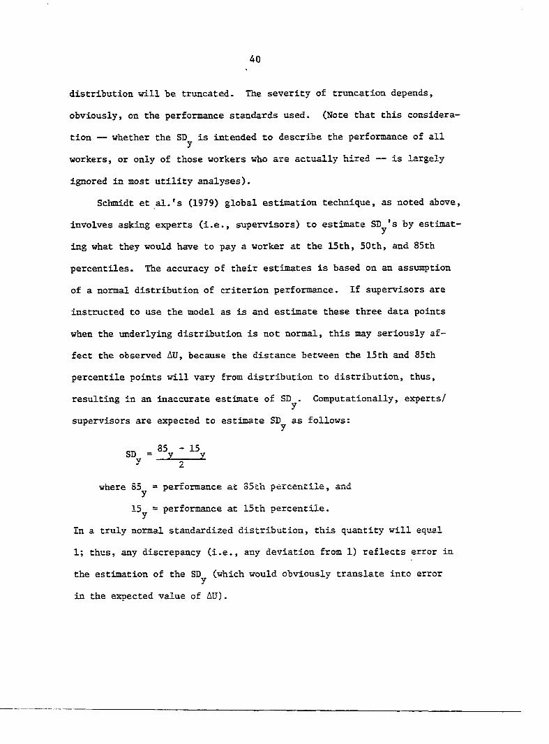
supervisors are expected to estimate SD^ as follows:

SDy = - 2

where 85^ = performance at SSth percentile, and

15y = performance at 15th percentile.

In a truly normal standardized distribution, this quantity will equal

1; thus, any discrepancy (i.e., any deviation from 1) reflects error in

the estimation of the SD^ (which would obviously translate into error

in the expected value of AU).

41

This can be graphically illustrated as follows:

In a normal distribution, the relevant area would be

+1(7 +2(7 +3(7 2<r 0 3ff lo­

in a truncated normal distribution, the area might vary from a

point at one standard deviation below the mean:

+10- +20- +3cr 0 lo­

to a point one standard deviation above the mean:

0 -3(7 -2(T -Iff +ia +2(7 +30"

Determination of the robustness of this term will be undertaken

in two separate steps. First, integral calculus will be used to ob­

tain the density function for any truncated normal distribution. This

density function will then be used to calculate the exact standardized

42

variance (and, hence, SD^') for a range of truncated normal distribu­

tions. This set of SD^'s will then be compared to 1 to assess the mag­

nitude of error in distributions that are progressively nonnormal.

4>/p

A second major analysis will involve an investigation of the term

reflecting performance on the predictor, $/p. As used in the model,

this term refers to the height of the normal curve at point £. More

generally, this refers to the average performance of the selected group

(i.e., those who meet or exceed the predictor cut-off). Note, however,

that if the distribution of predictor performance is not normal, this

specific term is inappropriate. In a nonnormal distribution, the height

of the curve at point ^ will reflect a different density (i.e., a dif­

ferent percentage of individuals beyond point £). This can be graphical­

ly illustrated as follows:

In a normal distribution of predictor performance, the organization

may decide to use £ = Û as the cutoff for accept versus reject. This

means that all those individuals in the shaded region would be considered

acceptable candidates:

+itr +2cr +3(7 0 -3(7 -20- -liT

43

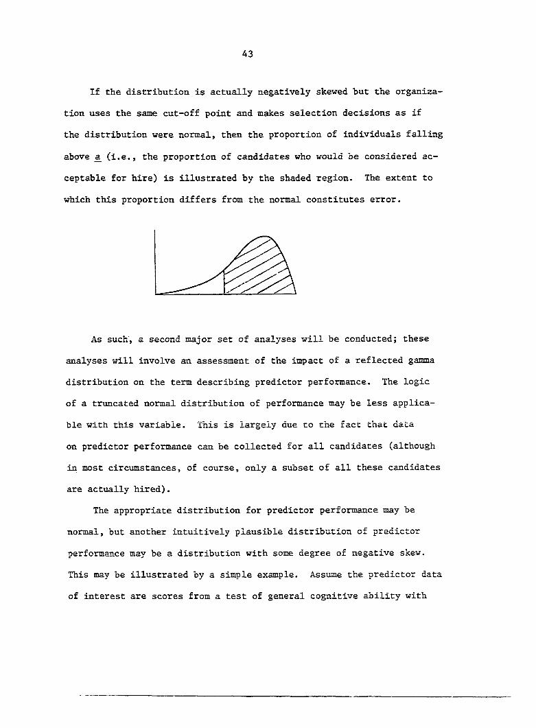
If the distribution is actually negatively skewed but the organiza­

tion uses the same cut-off point and makes selection decisions as if

the distribution were normal, then the proportion of individuals falling

above ̂ (i.e., the proportion of candidates who would be considered ac­

ceptable for hire) is illustrated by the shaded region. The extent to

which this proportion differs from the normal constitutes error.

As such, a second major set of analyses will be conducted; these

analyses will involve an assessment of the impact of a reflected gamma

distribution on the term describing predictor performance. The logic

of a truncated normal distribution of performance may be less applica­

ble with this variable. This is largely due to the fact that data

on predictor performance can be collected for all candidates (although

in most circumstances, of course, only a subset of all these candidates

are actually hired).

The appropriate distribution for predictor performance may be

normal, but another intuitively plausible distribution of predictor

performance may be a distribution with some degree of negative skew.

This may be illustrated by a simple example. Assume the predictor data

of interest are scores from a test of general cognitive ability with

44

performance normally distributed, where the mean is 100 and standard

deviation is 15. Although technically, if the organization had access

to a large enough (and heterogeneous enough) sample, the observed dis­

tribution might approach normal, it is unlikely that a normal distribu­

tion would be found in actual practice. It is unlikely, for instance,

that few (if any) candidates with scores of 70 and below would be part

of the applicant pool. In other words, relatively few scores would

be found at the low end of the scale, while more would probably be found

at the high end of the scale.

In more straight-forward terms, this means that the pool of avail­

able applicants might consist of a group of individuals dominated by

high performers, with a progressively smaller proportion of poor per­

formers. Because this type of distribution (that is, a negatively

skewed distribution) is difficult to specify by an exact mathematical

function, a solution may be to use a "reflection" (that is, a mirror

image) of a positively skewed distribution. Further, it may be useful

to specify that the "reflected" distribution must share the same mean

and variance as the standard normal distribution to permit more accurate

comparison.

This set of analyses will involve use of the probability density

function for an appropriate distribution. In a normal distribution,

this is equal to

6(%) = ̂ /2ir

45

An appropriate distribution for comparison might be a reflected

gamma distribution with mean of 0 and variance of 1. The probability

density function for this distribution is equal to

f (X) = ^ , X < a, a > 0, a = a^

Note that this term is directly analagous to selection ratio, as it

refers to the expected standardized score of those who are actually

selected. When interpreted in the context of selection, this may not

appear intuitively reasonable at first glance, as most analyses of

"utility" in this context incorporate the selection ratio itself (i.e.,

the number hired out of the total number of candidates) in some form.

Schmidt et al. (1979) note, however, that in most situations, the num­

ber of individuals to be hired is fixed by organizational constraints

and, hence, is not under the control of the employer. As such, it may

be mors conceptually meaningful to use the notion of expected score,

rather than expected percentage to be hired. Thus, rather than saying

"we expect to hire about 50% of all applicants" it may be more accurate

to say "we expect to hire those whose performance on the predictor is

at or above the group mean."

Full Model

After a determination of the robustness of these two individual

terms, it may be informative to examine the magnitude of error result­

ing from the use of incorrect estimates for each term. As such,

46

another analysis will involve calculating the expected error at various

combinations of the truncated SD distributions and different selection y

standards with a distribution of predictor performance that is negative­

ly skewed. To allow for straight-forward interpretation, the results

will be reported in terms of expected marginal increase in standardized

utility given different distributions of job performance and different

selection standards. Such an analysis is important to determine the

impact of varying selection standards given different distributions of

criterion performance on the expected increase in standardized job per­

formance.

47

RESULTS

In order to best understand and interpret the results, they will

be presented separately for SD^ and <j)/p, and then for the utility func­

tion as a whole.

SD y

A critical first step in assessing the robustness of the SD^ term

involves the variance (on which, of course, the standard deviation is

based) for a nonnormal distribution. In this case, the nonnormal dis­

tribution of interest is the truncated normal distribution, as described

above.

The standard normal density is

*(z) = — exp^"^

and the cumulative distribution function (cdf) is

' X $(x) = ({)(u)du , where $(x) = 1 - $(-x) for all x > 0.

If

$ (x) = y , then ô(y) = x

2 It is thus necessary to calculate the variance of the truncated

48

normal distribution, with density

<Î'(Ç)

0 for X < ca

The mean is not zero:

E(x) = j X <j)^(x)dx =

o f I *(2)̂

(LET • F • "" ° T'

ca

a r ̂ $Wdu

$(-c) Ç. _ a$(c)

$(-c) $(-c)

Similarly,

E(x^) =

i r 2 .X.2 ,x. dx

2 , , „ a ca •=' L ~

ca

2 f<» r 2 J u- $tu;du .

Now J x^ $(x)dx = - X 4)(x) + / ({)(x)dx, so

J *(u)du = (-u<p(u) cj)Cu)du) •" c

$( r (0 + c(j)(c) + 0(-c)) -c;

49

Since lim a 4)(a) = 0 a-x»

Thus

V(X) = OF = E(X^) - (E(X))^ = A^(L +FÎ^) o2($(c))2

(9(-c))Z

From this, it follows that the variance of a normal distribution with

Given this, the Statistical Analysis System (SAS) was used to cal­

culate the standard deviations of truncated noznnal distributions. (Note

that in a standard normal distribution, this quantity equals 1; thus,

any deviation from 1 indicates error.) The results of this analysis are

described in Table 1, where the point of truncation refers to the spe­

cific point at which the standard normal distribution (of job performance)

is truncated, % of employees eliminated refers to the percentage of em­

ployees who would fall below that point and, hence, would be eliminated

2 mean of 0 and variance of a that is truncated below at ca is

50

Table 1. The effects of distributional truncation on percentage of employees eliminated, SD , and error

Point of % of employees truncation eliminated SD^ Error

-4.00 00.003 1.0364 .0364

-3.75 00.009 1.0363 .0363

-3.50 00.020 1.0361 .0361

-3.25 00.050 1.0356 .0356

-3.00 00.130 1.0344 .0344

-2.75 00.30 1.0320 .0320

-2.50 00.62 1.0273 .0273

-2.25 01.22 1.0186 .0186

-2.00 02.28 1.0039 .0039

-1.75 04.01 0.9810 -.0019

-1.50 06.68 0.9490 -.0510

-1.25 10.56 0.9069 -.0931

-1.00 15.87 0.8565 -.1435

-0.75 22.66 0.8004 -.1996

-0.50 30.85 0.7412 -.2588

-0.25 40.13 0.6821 -.3179

0.00 50.00 0.6252 -.3748

0.25 59.87 0.5718 -.4272

0.50 69.85 0.5228 -.4772

0.75 77.34 0.4784 -.5216

51

Table 1. continued

Point of % of employees truncation eliminated SD

y Error

1.00 84.13 0.4386 -.5614

1.25 89.44 0.4031 -.5969

1.50 93.32 0.3716 -.6814

1.75 95.99 0.3436 -.6564

2.00 97.72 0.3188 -.6812

2.25 98.78 0.2968 -.7032

2.50 99.38 0.2771 -.7229

2.75 99.70 0.2596 -.7404

3.00 99.87 0.2438 -.7562

3.25 99.94 0.2297 -.7703

3.50 99.97 0.2170 -.7830

3.75 99.99 0.2054 -.7946

4.00 99.99 0.1950 -.3050

(i.e., at a point of truncation 4 standard deviations below the mean of

job performance, 0.003% would be eliminated for unsatisfactory per­

formance), and SDy refers to the standard deviation of performance in

standard score units. Since in a standard normal distribution this

equals 1, error refers to the difference between the SD^ for the trun­

cated normal distribution and 1.

52

<|)/p

The next critical step concerns the robustness of the ({)/p term,

which describes performance on the predictor. As such, let be gamma

distributed with probability density function

Since

and

a a-1 -az _ f ( z ) = , z > 0 , a > 0 , a = a

a W; " I " a

Oz = = 1 '

if we let X = a - z. (where x refers to predictor performance), then

= a - Mg = u

ana

2 2 1 °x = *z = 1

The parameter a refers to the top standardized score of those accepted.

Consequently, is standardized; it is also negatively skewed. The

distribution of JC will be referred to as a reflected gamma. (Note that

equality of a specific number of parameters — here, equality of means

53

and variances — is essential for the use of this distribution as a

location scale family, which refers to a family of distributions which

may vary in shape but share some specified number of parameters.) Use

of this reflected gamma distribution in particular allows us to assess

the effect of a negatively skewed distribution of predictor performance —

that is, a distribution where the relative density increases as predictor

performance increases. (Note that this would be descriptive of a hiring

procedure where better candidates have a better chance of being hired.)

Although the means and variances of these two distributions are

equal, the distributions have different shapes, which means that at

given points along the baselines, a different density (i.e., proportion

of individuals who are judged to be candidates acceptable for hire) will

fall beyond that point. This is obvious from the following results,

where ̂ refers to the top standardized score of those accepted (i.e.,

if £ = 2, then the top standardized score of those accepted will be two

standard deviations above the mean); NORDEN refers to the percentage

of cases falling beyond point _a in a normal distribution, and GAMDEN

refers to the percentage of cases falling beyond point a in a reflected

Gamma distribution. These two distributions are graphically illustrated

on the following page, where the dotted line indicates a normal distribu­

tion and the solid line indicates a gamma distribution. The horizontal

axis refers to the scale of predictor performance, and the vertical

axis refers to the density (i.e., the proportion of candidates) at a

given point.

54

Table 2. Comparison of percentage falling above lowest acceptable stand­ardized score in normal versus reflected gamma distributions

a NORDEN GAMDEN

2 02. 275 00. 710

1.5 06. 681 01. 334

1.0 15. .866 02. .499

0.5 30. .854 04. .594

0.0 50. .000 08. .298

-0.5 69. .146 14. .649

-1.0 84, ,135 25, .079

-1.5 93, .319 41, .135

-2.0 97, .725 63 .277

Combined Analyses

While the first two sets of analyses are informative in terms of

helping to assess the robustness of the SD^ term and the (|)/p term sepa­

rately, they are insufficient in determining the robustness of the utili­

ty function as a whole. As such, an analysis concerning the multiplica­

tive effect of these two terms (i.e., nonnormality in either or both)

is necessary.

The following two tables describe expected marginal utility with

(^2 - 22) equal to 0.10. (Note that any variation in N, which is here

set equal to one, and in the difference in validities would simply change

55

Figure 3. Normal (dotted) versus reflected Gamma- (solid) distributions of predictor performance (Note: Horizontal axis represents standardized predictor performance. Vertical axis repre­sents the likelihood of a point on the horizontal axis)

56

all of these estimates by that factor. For example, if N was equal to

50, then all the entries would simply be multiplied by 50.) Table 5 is

simply the difference between Tables 3 and 4.

The entries may be interpreted as follows. The columns refer to

progressively more stringent requirements for hire, with ̂ in column 1

equal to -2, and ̂ in column 9 equal to 2. In more straightforward

terms, this may be understood as follows. As noted above, a^ refers to

the top standardized score (of those accepted for hire) on the predictor.

With ja = -2, the top standardized score is two standard deviations be­

low the mean, meaning that standards for acceptance are relatively low.

As a increases, the organization's standards for acceptance increase

(i.e., only those who score progressively better on the predictor will

be accepted for hire). This table assumes that the distribution of pre­

dictor performance is normal, while the next table is based on a re­

flected gamma distribution of predictor performance.

The rows in both tables refer to progressively more stringent stand­

ards for job performance, with (point of truncation of the normal

distribution) equal to -4.00 in row 1 and 4.00 in row 33. This means

that, in row i, an employee's job performance must be 4 standard devia­

tions below the mean in order for that employee to be eliminated from

the organization, while in row 33, all employees whose performance is

4 standard deviations above the mean or "worse" are eliminated. In

other words, this means that in row 1, the organization's standards for

what constitutes acceptable job performance are relatively low (i.e..

57

an employee's performance must be considerably below the mean if that

employee is to be dropped), while in row 33, the organization's stand­

ards for acceptable job performance are extremely high, with only those

employees whose job performance is 4 or more standard deviations above

the mean being retained. The entries themselves refer to the expected

marginal (that is, per employee) increase in standardized utility. This

represents a relatively straightforward means of assessing "utility"

under different distributional assumptions. While it does not provide

a monetary estimate, such an estimate may be difficult to interpret at

this stage of exploration. In other words, before any attempts to gen­

erate dollars-and-cents estimates of the savings/profits that may accrue

from a change in human resources practices, it is necessary to generate

estimates which are not bound by such variable constraints as infla­

tion, costs of testing, etc.

The estimates represent a substantial refinement over earlier ef­

forts to assess utility, such as the Taylor-Russell tables. The unique­

ness of these estimates concerns their emphasis on the effects of dif­

ferent distributions of predictor and criterion performance. IJhile the

underlying mathematics are somewhat imposing by conventional professional

standards, they are critical in accurately assessing the stability of

the utility function in terms of potential departures from theoretical

assumptions and, hence, are an important step on the road to accounta­

bility in human resources cost accounting.

Table 3. Increase in marginal standardized job performance with a normal distribution of predictor performance and increasing truncation of job performance^

a

C

-2 -1.5 -1.0 -0.5

-4.0 0.246 0.201 0.158 0.118 -3.75 0.246 0.201 0.158 0.118 -3.50 0.246 0.201 0.158 0.118 -3.25 0.246 0.201 0.158 0.118 -3.00 0.246 0.201 0.158 0.118

-2.75 0.245 0.200 0.157 0.113 -2.50 0.244 0.199 0.157 0.117

-2.25 0.242 0.197 0.155 0.116 -2.00 0.238 0.194 0.153 0.115

-1.75 0.233 0.190 0.150 0.112 -1.50 0.225 0.184 0.145 0.108

-1.25 0.215 0.176 0.138 0.103 -1.00 0.203 0.166 0.131 0.098

-0.75 0.190 0.155 0.122 0.091 -0.50 0.176 0.144 0.113 0.085 -0.25 0.162 0.132 0.104 0.078 0.00 0.148 0.121 0.095 0.071 0.25 0.136 0.111 0.087 0.065 0.50 0.124 0.101 0.079 0.060 0.75 0.114 0.093 0.073 0.055 1.00 0.104 0.085 0.067 0.050 1.25 0.096 0.078 0.061 0.046

1.50 0.088 0.072 0.057 0.042 1.75 0.082 0.067 0.052 0.039

2.00 0.076 0.062 0.049 0.036 2.25 0.070 0.058 0.045 0.034

2.50 0.066 0.054 0.042 0.032 2.75 0.062 0.050 0.040 0.030 3.00 0.058 0.047 0.037 0.028 3.25 0.055 0.045 0.035 0.026

3.50 0.051 0.042 0.033 0.025 3.75 0.049 0.040 0.031 0.023

4.00 0.046 0.038 0.030 0.022

^The variable a represents expected top standardized score of pre­dictor performance given that predictor performance is normally dis­tributed. The variable C represents the point at which the normal distribution of job performance is truncated.

59

0.0 0.5 1.0 1.5 2.0

0.083 0.053 0.030 0.014 0.006

0.083 0.053 0.030 0.014 0.006 0,083 0.053 0.030 0.014 0.006

0.083 0.053 0.030 0.014 0.006 0.083 0.053 0,030 0.014 0.006

0.082 0.053 0.030 0.014 0.006 0.082 0.052 0.030 0.014 0.006

0.082 0.052 0.029 0.014 0.006 0.081 0.052 0.029 0.014 0.006 0.078 0.050 0.028 0.014 0.005 0.076 0.048 0.027 0.013 0.005

0.072 0.046 0.026 0.013 0.005

0.068 0.043 0.025 0.012 0.005 0.064 0.041 0.023 0.011 0.004

0.059 0.038 0.021 0.010 0.004 0.054 0.035 0.020 0.009 0.004

0.050 0.032 0.018 0.009 0.003 0.047 0.029 0.016 0.008 0.003

0.042 0.027 0.015 0.007 0.003 0.038 0.024 0,014 0.007 0.003

0.035 0.022 0.013 0.006 0.002 0.032 0.021 0.012 0.006 0.002

0.030 0.019 0.011 0.005 0.002 0.027 0.017 0.010 0.005 0.002 0.025 0.016 0.009 0.004 0.002

0.024 0.015 0.009 0.004 0.002 0.022 0.014 0.008 0.004 0.002

0.021 0.013 0.007 0.004 0.001

0,019 0-012 0.007 0.003 0.001

0.018 0.012 0.007 0.003 0.001 0,017 0.011 0.006 0.003 0,001

0.016 0.011 0,006 0.003 0.001

0.016 0.010 0.006 0,003 0.001

Table 4. Increase In marginal standardized job performance with a reflected gamma distribution of predictor performance and increasing truncation of job performance^

a —2.0 —1.3 —1.0 —0.5

C

-4.0 0.080 0.081 0.082 0.082

-3.75 0.080 0.081 0.082 0.082

-3.50 0.080 0.081 0.082 0.082

-3.25 0.080 0.081 0.082 0.082

-3.00 0.080 0.081 0.082 0.082

-2.75 0.080 0.081 0.081 0.082

-2.50 0.079 0.080 0.081 0.082

-2.25 0.079 0.080 0.080 0.081

-2.00 0.078 0.078 0.079 0.080

-1.75 0.076 0.077 0.077 0.078 -1.50 0.073 0.074 0.075 0.075

-1.25 0.070 0.071 0.071 0.072 -1.00 0.066 0.067 0.067 0.068

-0.75 0.062 0.063 0.063 0.064

-0.50 0.057 0.058 0.058 0.059

-0.25 0.053 0.053 0.054 0.054 0.00 0.048 0.049 0.049 0.050

0.25 0.044 0.045 0.045 0.045

0.50 0.040 0.041 0.041 0.042

0.75 0.037 0.037 0.038 0.038

1.00 0.034 0.034 0.035 0.035

1.25 0.031 0.031 0.032 0.032

1.50 0.029 0.029 0.029 0.030

1.75 0.027 0.027 0.027 0.027

2.00 0.025 0.025 0.025 0.025

2.25 0.023 0.023 0.023 0.024

2.50 0.021 0.022 0.022 0.022

2.75 0.020 0.020 0.020 0.021

3.00 0.019 0.019. 0.019 0.019

3.25 0.018 0.018 0.018 0.018

3.50 0.017 0.017 0.017 0.017

3.75 0.016 0.016 0.016 0.016

4.00 0.015 0.015 0.015 0.015

^The variable a represents expected top standardized score of predictor performance is distributed as reflected gamma. The variable C represents the point at which the normal distribution of job per­formance is truncated.

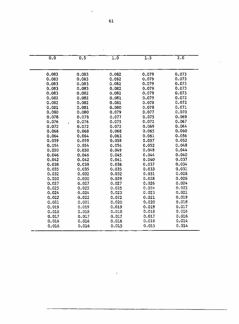
61

0.0 0.5 1.0 1.5 2.0

0.083 0.083 0.082 0.079 0.073 0.083 0.083 0.082 0.079 0.073 0.083 0.083 0.082 0.079 0.073

0.083 0.083 0.082 0.079 0.073 0.083 0.082 0.082 0.079 0.073 0.082 0.082 0.081 0.079 0.072 0.082 0.082 0.081 0.078 0.072

0.081 0.081 0.080 0.078 0.071 0.080 0.080 0.079 0.077 0.070

0.078 0.078 0.077 0.075 0.069 0.076 0.076 0.075 0.072 0.067

0.072 0.072 0.072 0.069 0.064 0.068 0.068 0.068 0.065 0.060

0.064 0.064 0.063 0.061 0.056 0.059 0.059 0.058 0.057 0.052

0.054 0.054 0.054 0.052 0.048 0.050 0.050 0.049 0.048 0.044

0.046 0.046 0.045 0.044 0.040 0.042 0.042 0.041 0.040 0.037

0.038 0.038 0.038 0.037 0.034

0.035 0.035 0.035 0.033 0.031 0.032 0.032 0.032 0.031 0.028

0.030 0.030 0.029 0.028 0.026 0.027 0.027 0.027 0.026 0.024 C • 025 C. 025 0.024 0 = 022 0.024 0.024 0.023 0.023 0.021

0.022 0.022 0.022 0.021 0.019 0.021 0.021 0.020 0.020 0.018

0.019 0.019 0.019 0.019 0.017 G. OIS 0.018 G. OIS 0.018 0.016

0.017 0.017 0.017 0.017 0.016 0.016 0.016 0.016 0.016 0.014

0.016 0.016 0.015 0.015 0.014

Table 5. Absolute marginal error in the use of the theoretical normal versus the empirical reflected gamma distribution^

a

C

-2.0 -1.5 -1.0 -0.5

-4.00 -0.166 -0.120 -0.076 -0.036 -3.75 -0.166 -0.120 -0.076 -0.036 -3.50 -0.166 -0.120 -0.076 -0.036 -3.25 -0.166 -0.120 -0.076 -0.036

-3.00 -0.165 -0.120 -0.076 -0.036 -2.75 -0.165 -0.119 -0.076 -0.036

-2.50 -0.164 -0.119 -0.076 -0.036 -2.25 -0.163 -0.118 -0.075 -0.035

-2.00 -0.160 -0.116 -0.074 -0.035 -1.75 -0.157 -0.113 -0.072 -0.034

-1.50 -0.152 -0.110 -0.070 -0.033

-1.25 -0.145 -0.105 -0.067 -0.031 -1.00 -0.137 -0.099 -0.063 -0.030

-0.75 -0.128 -0.093 -0.059 -0.028 -0.50 -0.119 —0.086 -0.055 -0.026

-0.25 -0.109 -0.079 -0.050 -0.024 0.00 -0.100 -0.072 —0.046 -0.021

0.25 -0.091 —0.066 -0.042 -0.020 0.50 —0.084 -0.061 -0.039 -0.018

0.75 -0.077 -0.055 -0.035 -0.017 1.00 -0.070 -0.051 -0.032 -0.015

1.25 -0.064 -0.047 -0.030 -0.014 1.50 -0.059 -0.043 -0.027 -0.013

1.75 -0.055 -0.040 -0.025 -0.012 2.00 -0.051 -0.037 -0.023 -0.011

2.25 -0.047 -0.034 -0.022 -0.010 2.50 -0.044 -0.032 -0.020 -0.010

2.75 -0.042 -0.030 -0.019 -0.009 3.00 -0.039 -0.028 -0.018 -0.008

3.25 -0.037 -0.027 -0.017 -0.008

3.50 -0.035 -0.025 -0.016 -0.008 3.75 -0.033 -0.024 -0.015 -0.007

4.00 -0.031 -0.023 -0.014 -0.006

^(**** indicates that the difference was <0.00 and, hence, is not reported.) The variable a refers to the expected top standardized score of predictor performance given that predictor performance is dis­tributed as a reflected gamma. The variable C represents the point of which the normal distribution of job performance is truncated.

* x- >!• X- X- X- X- H- * * * * » * X- X- X- X- X- X- X- x- X- î X- * » X- * » X* *. X- » *- X- X- » M- * * * * » * X" X- x- X- X- X- x- X- X- X- x- X- X- } X- X" X-

X- x- H- X- X- X- X- X- » * » » » X- » * X- X- X- X- x- X- x- x< x- î * 5 * » * X* * *- *- » * *- M- * * *- * * X- * X- X- X- X- X" x- X- x- x- * x- x- X- X- x- X- X- X-

o o

o o o o

0 o o o O o O o O O o o o o O O o o O o o C) O O o o o o o

o o a> o o m

o o cr> o o -4

.007

o o o o 00

o o VO O O VO

O H O O p o H K> ? w o g o G o M o\ o H 00 o N O

O ts> M

S W o to Ul b ON

o ro h

00 o ro VO 8 V£)

O W O O w o o w o o w o

s o

s o o i j i o

o Ln

o o o o o o o o o o o o o o o o o o o o o o o o o o o o o o o o o

O O M W h J W 4 > L n ( T % ^ v O O h J ^ C T \ ( % ) 0 0 ~ ^ ^ O W L n O O \ O O H ^ M N ) N ) N N ) N N )

m U)

o o o O O O O O O O O o o o o o o o o o o O O O O

0.

O O o O O O O

o o o o O O O O O O O o o o o o o o o o ô P P O O O O O o O O O O M M h-» M I—* H H M to to to ro to w w w w Ln Ln Ln Ln On ON Ch ON ON ON P ON ON On

to w 4N 4S Ln On kO O H w Ui VJ o w o\ o> w o LO VO H W 4> -p> Ln Ln Ln Ln Ln Ui

O O O O

O O O O O O O O O O o o O O O o O O O O o O o

0.

O o o O o o o

O O O O O O O O o O o o O O o o O O O p O Ô o O o o o O o o o M H H H M H t o t o t o t o t o u > w W 4 > Ln Ln Ln on on on on on on On on on on On

4 > Ln on 00 kO H t o on 00 M 4N o 00 t o Ln VO H w Ln on on •vj *vj

N O

64

DISCUSSION

In order to understand the importance of the foregoing analyses,

it is necessary to examine the two most important variables — SD^ and

ç/p — separately, before considering the implications of the results

in terms of the applicability of the function as a whole. Because all

other terms in the function (such as N, and C^, and the r^ - ̂ 2 dif­

ference) are simply multiplicative factors, these two terms are ob­

viously most critical in terms of assessing the function's robustness,

and, hence, are essential as a first step in determining the tenability

of its use in an applied setting.

Statistical implications

As noted above, SD^ is intended to reflect/describe the distribu­

tion of job performance in the organization. Before discussing more

specific implications of this term in an organizational context, however,

it may be useful to consider the importance of the standard deviation

in a statistical sense.

In precise statistical terms, the standard deviation is a measure

of spread or dispersion of scores around the average, or most typical

score — in other words, a term frequently used in descriptive statistics

to help describe the relative amount of variability in a particular dis­

tribution of scores. Mathematically, it is the square root of the vari­

ance, where the variance is equal to

65

n _ « Z (y. - y) i=l ^

n — 1

for "small" a (i.e., less than 30) and

° 2 z (y. - M) i=l ^

n

for "large" n.

The variance is a "unit-bound" measure of variability. This means

that unless the distribution of interest has been standardized (that is,

converted to a scale where the arithmetic mean is equal to 0 and the

variance is equal to 1), the SD^ cannot be interpreted without reference

to the particular scale used in the underlying distribution, as the

significance of any particular standard deviation can be evaluated only

in terms of its relationship to the distribution being used. This, again,

is the rationale for expressing the SD^ in standard score units as a more

precise measure of the absolute, or cardinal (rather than relative, or

ordinal) utility expected to result from a particular decision. This

kind of approach will allow an estimate of SD that is not unit-bound and,

hence, can be interpreted without reference to some arbitrary scale of

pay.

The meaning of SD^ can best be understood by careful examination

of the deviation-score formula:

66

2 z (y. - u) 1=1 ^

n

Obviously, the SD^ reflects the amount of variation or "spread" around

the mean (i.e., the most typical) score. In terms of job performance,

it refers to the dispersion of performance (for a group) around average

performande. As noted above, a number of classic referents (i.e.,

Munsterberg, 1914; Hull, 1928) had pointed out that performance within

a particular job will vary across people. This reflects the obvious

fact that merely determining the average, or most typical, level of job

performance is insufficient to accurately describe the performance of

the employee group as a whole.

The most extreme case investigated here (mainly for purposes of

comparison) concerns the rectangular distribution, also known as the

distribution of constant density. In statistical terms, this refers to

a density of the function

p(x) = Y ifb--ra<x<b+-|-a

0 otherwise

in more general terms, this means that the same proportion of employees

would be found at every level of job performance, rather than a larger

proportion at or near the mean, with the frequency decreasing at points

67

further above and below the mean. The SD^ for a standardized rectangu­

lar distribution Cas calculated by Schmidt et al.'s global estimation

technique) differs from by approximately 25%.

Note that, technically speaking, the distribution of constant den­

sity does not represent the most extreme departure from a normal distri­

bution that is possible; this would be the case with an inverted U-shaped

distribution, more precisely called a hyperbolic distribution. However,

it is difficult, if not impossible, to conceive of a real-life situation

where the distribution of job performance could be appropriately described

as hyperbolic, as this would be analogous to assuming that the smallest

proportion of workers fell at a point describing average job performance,

with increasingly larger proportions at points further above and below

the mean (i.e., more "excellent" and "poor" workers than "average"

workers. Because it is so unlikely that such a distribution would be

found in an actual organizational setting, it was felt that investiga­

tion of the impact of this type of distribution on estimates of SD^ would

have relatively little meaning, in either conceptual or practical terms.

The utility function assumes that the distribution of job performance

is approximately normal. (Although Schmidt at al., 1979, argus that

this assumption is largely for derivational purposes, an inspection of

the distributional assumptions used in every investigation of the use of

utility function in human resources indicates that the assumption of

normality is widely accepted.) In statistical terms, this means that

the distribution is roughly equal to 0, where $ refers to the density

68

function of the normal distribution

p(x) = — exp^"^

In more general terms, this means that not only is the distribution

of performance symmetrical (i.e., there are as many performers below the

mean as above, and the performance of the best employees is "balanced"

by that of the worst), but that a fixed and predictable proportion of

individuals falls into specific intervals of the distribution. For ex­

ample, the distribution could accurately be described in terms of stand­

ard deviations by virtue of the fact that roughly 58% of the population

is within 1 standard deviation of the mean. In other words, if the dis­

tribution of job performance is approximately normal, roughly 34% of the

population will be within 1 standard deviation above the mean, and rough­

ly 34% will be within 1 standard deviation below the mean. As performance

moves in either direction away from the mean, fewer and fewer employees

will fall at these increasingly more extreme points of job performance.

If job performance in an organization actually is normally dis­

tributed, 0 = O where a refers to the standard deviation of the normal ne n

distribution and refers to the standard deviation of the empirical

distribution. However, in most real-life situations, organizational

constraints preclude a truly symmetrical distribution of performance.

It is simply not tenable to imagine that all performers, even the very

poorest, will remain with the organization; typically, the organization

69

is forced to jettison such employees for their failure to contribute to

the attainment of organizational goals.

Note that, according to Lehman (1975), the distribution of measure­

ments taken under sufficiently well-controlled conditions is often ap­

proximately normal; thus, this observation is reasonable in many organi­

zational settings. Lehman also points out, however, that while it was

formerly believed that the normal distribution is practically universal

as a distribution of measurements, it has since been determined that this

tends to be true only for the central part of the distribution, with the

tails often being distorted by mistakes in measurement or other excep­

tional circumstances — so-called gross errors. The implication is

that the normal distribution may not necessarily be the most accurate

description of the empirical distribution.

Young and Veldman (1977) note that if a distribution is highly

skewed, the variance (and, hence, the standard deviation) is not the

best measure of variability, largely because scores are squared in the

computation of the variance. This means that extreme scores are weighted

much more heavily than are scores near the mean. The overall effect

would be a marked (and possibly misleading) increase in the observed

standard deviation due to relatively few extreme scores. Young and

Veldman contend that the semi-interquartile range, which is defined as

half the distance between the point below which 25% of the observations

and the point below which 75% of the observations fall, is the pre­

ferred measure of variability in a skewed distribution. Since the

70

values of the extreme observations have little effect on the semi-inter-

quartile range, it is more appropriate than the variance in a highly-

skewed distribution.

In statistical terms, a finding more realistic than a normal dis­

tribution might be a truncated normal distribution, with some propor­

tion of the left tail cut off Cthe specific point of truncation being

determined, obviously, by the organization's standards for job per­

formance). Statistically speaking, this is referred to as a skewed

distribution; if some portion of the left tail (i.e., the portion below

the mean) is cut off, the skew is described as positive, because the

"tail" (more precisely, the long part of the distribution) points towards

the high, or positive end of the scale of job performance.

When described in terms of skewness, this type of distribution may

seem conceptually illogical at first glance, because it appears that

there are more employees clustered at the low end of the performance

scale, with the relative proportion of employees falling off at higher

levels of job performance. In other words, it may appear that a larger

proportion of employees perform at a relatively lower level, compared to

the proportion who are performing at a relatively high level. It must

be kept in mind, however, that even job performance at the extreme left

of the truncated normal distribution (i.e., at the low end of the per­

formance scale) represents performance deemed acceptable by the organi­

zation's standards. There is, thus, a pile-up of scores on the low end

of this modified scale, but the pile-up involves a scale on which all

71

performance is at least minimally acceptable.

From a statistical perspective, it is necessary to first examine

the effects of this truncation on where = the standard deviation

of the truncated normal distribution as estimated by the Schmidt et al.

(1979) global estimation technique. In terms of computational clarity,

SDy is equal to (85^ - 15^)/2, where 85^ refers to performance at the

85th percentile, and 15^ refers to performance at the 15th percentile.

In a standard normal distribution, this quantity would obviously be

equal to 1.

Substantive implications

In more general terms, this can be understood as follows. Assume

that if an organization was able to retain all those initially hired,

the resulting distribution of job performance would, indeed, be ap­

proximately normal. However Cas noted above), in terms of organization­

al effectiveness, it is reasonable to assume that extremely poor job

performance is detrimental to the attainment of organizational objectives.

It is, therefore, logical to assume that there would exist some minimum

cut-off point, meaning that at some point, job performance would no

longer be considered acceptable, and all individuals whose job performance

fell below that point would be terminated. This minimum cut-off point

would, thus, cause a truncation of the normal distribution because some

portion of the left tail (the specific portion depending, obviously, on

the exact placement of the cut—off point), would drop out of the distribu­

tion. If the cut—off point was placed far below the mean of job per­

formance, only a very small portion of the employees would be eliminated.

72

and the resulting distribution of job performance would largely re­

semble a normal distribution. However, as the cut-off point was moved

up the scale of job performance (meaning that as the minimm standard

for "acceptable" job performance was made more stringent), the distribu­

tion would become increasingly more truncated and decreasingly like the

normal distribution.

Conceptually, it is logical to assume that as the range of job

performance varies from a normal distribution, so too would the esti­

mate of SD differ from 1. As is obvious from the results described y

above, this is, indeed, what happens. IJhen the cut-off point is set at

a point approximately two standard deviations below the mean, the effect

on (i.e., in comparison to a^) is negligible. This is equivalent

to eliminating roughly the lowest 2.5% of the total employee population.

As the cut-off is set at progressively higher points (i.e., moved up the

scale of job perfoinaance towards the mean), the impact on (again,

as compared to a^) becomes progressively more significant. At a point

two standard deviations below the mean, differs from by a factor

of less than one percent, while at a point one-half standard deviation

below the mean, it differs by 25%. (As noted above, SD^ as estimated by

this approach should be approximately equal to 1; any deviation from 1,

either over or under, indicates the presence of error.)

Careful inspection of the results for SD^ with a truncated normal

distribution indicates that at relatively small deviations from the

normal distribution, very little error in the estimation of SD is in­

73

volved. Between = -4 and = -1.65, the magnitude of error Cin terms

of the truncated normal distribution as compared to the normal distribu­

tion) is ± 3%. At extreme points of truncation, however, the magnitude

of error becomes considerably more pronounced.

Also, note that at very extreme mpoints of truncation (i.e., at

or above the mean), the impact on SD^ is quite substantial; however,

this is analogous to the elimination of those whose job performance is

average (or possibly even those whose performance is above average, de­

pending on the location of the truncation point) and, thus, would not

be a very realistic occurrence in most organizational settings.

Note that these manipulations are largely numerical in nature and

are based on the admittedly somewhat tenuous assumption that supervisors

can accurately assess SD^ themselves. In other words, the discrepancies

pointed out here involve discrepancies between accurate estimates of

SDy (as calculated by the global estimation technique) when the under­

lying distribution actually is normal and the same quantity when the

distribution is not precisely normal.

Another major potential source of error, besides the objective

error present in using an improper distribution of job performance (i.e..

assuming that the distribution in question is truly normal when, in fact,

it is a truncated normal) concerns the degree to which supervisors really

can make accurate estimates of SD^. Nisbett and Wilson (1977) argue that

the limitations of human introspection preclude an accurate examination

of thought processes. In other words, they contend that people general­

74

ly are not capable of describing, with, any degree of accuracy, how or

why they reached a particular decision. In the context of this inves­

tigation, it may be difficult to determine if supervisors can make ac­

curate estimates of that are based on actual job performance. In­

vestigation of this type of error in the context of this study, however,

would involve an analysis of the degree to which supervisors as subjects

can accurately report on their own decision-making processes (i.e.,

what factors or cues they use in evaluating the performance of employees

in monetary terms) and, hence, is beyond the scope of this study.

These results provide at least minimal evidence that the SD^ term

is relatively robust, and, hence, have important implications for the

use of the utility function in practical settings. Note that a number

of authors (Schmidt et al., 1979; Boudreau, 1983b; Landy & Farr, 1983)

have contended that a major obstacle to widespread use of the utility

function as a means of analyzing cost—benefit ratios of human resources

practices concerns the presumed difficulty of estimating SD^, the stand­

ard deviation of performance. Given the results of the first set of

analyses, it appears that the SC^ as determined by the global estimation

technique is at least somewhat impervious to departures from normality

in terms of the actual distribution of job performance. Further, if

an organization has some cognizance of their performance standards and

the resulting impact of such standards on the distribution of job per­

formance, they may be able to account for at least some departures from

normality in estimates of SD (and, therefore, in estimates of AU). y

75

«{"/p

Statistical implications

The second major variable of interest is 4Vp, where ^ refers

to the height of the normal curve at point In more general terms,

it refers to the expected score (on the predictor) of those who

are accepted. It would be very unusual for an organization to accept

all available candidates for hire; more typically some minimum predictor

score is established and only those whose performance on the predictor

meets or exceeds that are accepted for hire (given, of course,

that the exact number to be hired is determined by organizational con­

straints). If the performance on the predictor was, indeed, normally

distributed, then in a standardized distribution, the mean is equal to

0 and the standard deviation is equal to 1, and there would be a fixed

and predictable proportion of candidates falling above any arbitrary

predictor score. However, consider what happens when we take into ac­

count the fact that not all candidates are hired; and that the true dis­

tribution of predictor performance is not normal. As noted above, a

conceptually plausible distribution of predictor performance is a re­

flected gamma (F), where the density is specified by

a a-l -az 2 f(z) = ^ , z > 0, z > 0, a = a

This means that

u = — = a, and 7̂. a

76

(Note that equality of some number of parameters — here, equality

of mean and variance — is essential for the use of this distribution

as a location scale family, which refers to a family of distributions

which may vary in shape but share some number of parameters.)

As noted above, this means that the top standardized score is a^.

Consider the meaning of .a in this context. As we set the minimum ac­

ceptable predictor score at progressively higher points, the difference

between the maximum score and the mean score will of necessity decrease.

(Consider, for example, a test with a possible total of 100 points. If

50 is designated as the cut-off for acceptable performance, selectees

may fall anywhere in the interval from 50 to 100. If, however, 75 is

designated as the cut-off, acceptable candidates may fall only between

75 and 100.) This works to narrow the range of acceptable scores and

makes the empirical distribution progressively more different than the

theoretical distribution.

Note that practical constraints may preclude a distribution of

predictor performance that is exactly analogous to the normal distribu­

tion. This is because measurement devices may not be designed to account

for performance at all points in the interval ± infinity. However, given

that ± 2 standard deviations includes mere than 95% of the total dis­

tribution, this range is almost certainly acceptable for most applica­

tions.

77

Substantive implications

The implications of these analyses for usage of the model are as

follows. When an organization is determining some minimum acceptable

level of predictor performance, it is critical to consider the impact

of the ())/p term on utility estimates. (Note that this term is direct­

ly analogous to selection ratio, because as standards for acceptable

predictor performance increases, the selection ratio will of necessity

decrease, except under the highly unlikely condition that there is no

variability in terms of predictor performance among the available candi­

dates. To restate this in more meaningful terms, as the organization

becomes more selective — that is, sets the minimum cut-off for accept

versus reject at a higher point — the number and the proportion of

candidates who will be considered acceptable for hire will almost cer­

tainly decrease.)

The degree of error can be graphically illustrated by examining

the difference between the graphs GAMDEN and NORDEN in Figure 3.

It can be more precisely determined by examining the difference in den­

sity at any particular point as illustrated in Table 2. If, for example,

we examine the relative densities at a point where ̂ = 1, it is obvious

that there is a considerable amount of discrepancy between the two.

Note that this is to be expected given the difference in shape between

the two distributions. Even at a point where a^ = 2, however, the two

densities differ markedly. If it is assumed that the distribution of

predictor performance is normal, then the density at the point where

78

a = 1 would be assumed to be 15.8669; the corresponding density in a re­

flected gamma distribution is 2.49990. The "error" is not precisely

in the use of the normal distribution versus the reflected gamma dis­

tribution; rather, it is in the use of the d)/p term in the model. If

performance is normally distributed, then (j)/p (where ^/p reflects the

height of the normal curve at point 2 and, hence, describes a certain

portion of individuals beyond £) is correct. However, if the distribu­

tion is actually a reflected gamma shape (though still having a mean of

0 and a standard deviation of 1), the error will occur in terms of the

proportion of candidates expected to fall beyond 2-

At very low selection rates (i.e., where the organization has es­

tablished a relatively high cut-off for predictor performance), the im­

pact in terms of error may be substantial. At higher selection rates,

however, the impact becomes progressively less (although there will

always be some amount of error present unless the organization hires all

available candidates).

Schmidt et al. (1979) point out that in most situations, the number

of candidates to be hired is fixed by organizational constraints. The

selection ratio is largely determined by circumstances and is not under

the control of the ençloyer. In circumstances where the applicant pool

is roughly constant, any statements concerning "optimal" selection ratios

have little practical value, since the selection ratio is not under the

control of the employer. For this reason, it is more intuitively meaning­

ful to discuss selection in terms of expected score than in terms of per­

centage of applicants hired.

79

General Implications

While the statistical machinations are of some interest, the most

important implications concern the overall impact of different distribu­

tions of predictor performance and job performance on AU. Because the

utility function is multiplicative, any error in the estimation of

various components would cause the resulting estimation of AU to be in

error by that percentage. In the case of the above analyses, an inter­

esting pattern of results is found.

The magnitude of error can be ascertained by an examination of

Table 5, which represents the difference between the marginal increase

in utility under the parameters of the reflected gamma distribution

(as shown in Table 4), and the same increase in utility under the as­

sumptions of the normal distribution (as shown in Table 3). A more

straight-forward way to interpret these results is as the difference

between what is actually true (the reflected gamma distribution) and

what the decision-maker believes to be true (the normal distribution),

When this difference is negative, this means that the decision-maker's

estimate of AU is too large (i.e., the actual increase in marginal

utility is smaller than what is assumed by the decision-maker). When

this difference is positive, the decision-maker's estimate of AU is

too small (i.e., relative to the actual increase in marginal utility

that would occur).

An inspection of Table 5 indicates that neither the direction nor

the magnitude of error is constant across various combinations of as­

80

sumptions. In terms of magnitude, the largest errors occur at high

selection ratios Ci.e., where a, the expected score on the predictor of

those hired, is relatively low) and low points of truncation of job

performance (i.e., where the organization's standard for what consti­

tutes acceptable able job performance is relatively low and, hence,

serves to eliminate only a very small portion of the employees).

For exasqile, in Table 5, row 1, column 1, the error is -0.166.

As increases (that is, as the organization's standards for acceptable

job performance increase), the difference decreases. The smallest

amount of error is obviously in the opposite half of the matrix, where

the organization has very high standards for acceptance and for job per­

formance, meaning that the expected score for those hired is high and

the standard for what constitutes acceptable job performance is also

high.

In terms of the direction of error, the differences are negative

(meaning that the decision-maker has overestimated the expected gain

in marginal utility) until column 5 (where ̂ = 0, meaning that the

top standardized score on the predictor is zero). In this column, the

differences are so small as to essentially equal zero. As a^ increases

(columns 6, 7, 8, and 9), the amount of error tends to increase somewhat,

although the error is now positive (meaning that the decision-maker

could be underestimating the utility of the proposed change).

Intuitively, these findings may be understood as follows. When ̂

is low, the top standard score of those accepted is low; thus, the

81

organization does not have high standards for the expected quality of

those accepted. When is low, the point of truncation for acceptable

versus unacceptable job performance is low, meaning that the organiza­

tion does not have high standards for what constitutes acceptable job

performance. It is, thus, understandable that, given low standards

for selection and for "good" job performance, a comparatively large

amount of overestimation occurs. In other words, it may appear to the

decision-maker that considerably more utility is expected than would

actually accrue; however, this may be due largely to very lax job stand­

ards. In the opposite situation, where standards for both acceptance

into the organization and acceptable job performance are high, the de­

cision-maker may tend to underestimate potential gains. (Note that,

although the gains themselves are smaller, this is due to the fact that

at very high standards, performance is already quite high; thus, it is

to be expected that there is some ceiling on performance and, hence, on

expected utility — i.e., on the amount that standardized job performance

can be expected to increase.)

In essence, the types of errors possible are not symmetrical and

obviously depend largely on existing conditions in the organization.

If standards for both selection and continued tenure are relatively

low (i.e., the organization has a high selection ratio and a low stand­

ard for what constitutes "acceptable" job performance), the relative

gains in standardized marginal utility (where utility refers, again,

to the expected increase in marginal standardized job performance) may

82

appear quite substantial. If the organization has high standards for

acceptance (i.e., hire) and for acceptable job performance, such rela­

tive gains may appear modest. This seemingly paradoxical finding is due

to the importance of the base rate of job performance. If standards

for selection and retention are low, the base rate of performance is

low; hence, there is a good deal of room for improvement in terms of

expected marginal increase in standardized job performance. If stand­

ards for selection are high and job performance is already relatively

high, then gains (relative to average current job performance) may be

smaller. (Note, however, that the expected average level of job per­

formance may still be higher even if the expected gains themselves are

relatively small.)

The logic of whether underestimation or overestimation occurs may

appear counter-intuitive at first, because if actual gains in utility

are smaller than estimated gains, the result is overestimation of

utility, not underestimation. The explanation, however, is as follows.

The use of the Schmidt et al. (1979) application assumes that the dis­

tributions of both predictor performance and job performance are normal.

In terms of the global estimation technique, this means that super­

visors are estimating SD^ as if the distribution is normal; hence, the

standardized SD^ is equal to 1. If, however, the true distribution of

job performance is not normal, the appropriate variance (and, hence, the

appropriate standard deviation) for a truncated normal distribution is

less; thus, the empirical standard deviation is less. In other words.

83

supervisors may be estimating SD^ as if the empirical distribution is

normal when it is actually a truncated normal distribution. Note again

that the impact of AU is negligible at cut-off points that are far be­

low the mean of job performance. Similar logic may apply to the (j)/p

term. If the distribution of predictor performance is assumed to be

normal when it is actually more similar to a reflected gamma distribu­

tion, the proportion of individuals expected to meet or exceed the mini­

mum predictor cut-off is generally smaller than anticipated.

It is critical, however, for the organization to have at least a

rough idea of the shape of the performance distribution (for both pre­

dictor performance and job performance). This caveat stems from an in­

spection of Tchebysheff's theorem:

Given a number k > 1 and a set of n measurements, at least (k - l)/k of the measurements will lie within ̂ standard deviations of their mean.

For example, if n = 30 and k = 3, then

k — 1 = 2. and

k - 1 so at least 2/3 of the measurements will lie within 3 3 standard deviations of the mean; thus, at least 20

observations will lie within the interval ± 3 stand­ard deviations.

Though this was originally intended as a description of the variability

of a normal distribution, it has also been found to describe, reasonably

well, the variability of other mound-shaped distributions. (Note that

Mendenhall, 1983, points out that mound-shaped and bell-shaped distribu­

tions occur frequently in nature and, hence, Tchebysheff's theorem is

widely applicable.) Also, Tchebysheff's theorem gives a lower bound

84

as an estimate of the fraction of measurements falling within the

specified interval.

The implications of these analyses for implementation of the model

in human resources functions will depend, obviously, on value judgments

which must be regarded as somewhat arbitrary in nature. This concept

may be analyzed with respect to two important concepts: First, how

does the organization plan to use the results of a particular utility

analysis for decision making? For example, will a utility analysis be

conducted to determine whether or not a different type of selection

should be used to result in better average job performance? Similarly,

the organization may wish to estimate the expected gains in job per­

formance that may accrue from the implementation of a different type of

training program. Secondly, how can the magnitude of error be assessed

in terms of the ramifications for the organization?

Note that two completely different types of error are possible.

The organization may decide against a change when they should have de­

cided in favor of the change. Conversely, they may decide in favor of

a change when no such change was in fact warranted. For example, they

may decide, on the basis of a utility analysis, that a different

selection procedure would result in a substantial improvement in job

performance. If the assumptions underlying utility theory are not met,

however, these estimates of the expected increase in job performance

(expressed in standard score units or in monetary terms) indicate

more utility than would actually accrue is to be expected.

85

Conversely, the organization might decide, on the basis of another

utility analysis, that a proposed change in their selection system or

training program would not be warranted, given the apparent expected

gain in utility (i.e., increase in job performance). If their estimates

of the expected utility are underestimates, this is obviously an incor­

rect decision. The type of error that is preferable is, of course,

largely a question of value system. For example, would the decision­

maker prefer to forego potential monetary benefits or overestimate po­

tential monetary benefits?

The type of error that is more likely is obviously a question of

whether under- or overestimation has occurred. If the error is (un­

beknownst to the organization) on the side of conservatism, the organi­

zation may view the utility expected to result from the proposed change

with some caution or even pesssimism, because it may appear that the

monetary benefits predicted to result from change are modest or even

negligible. This may dissuade the organization from implementing change

when doing so would actually result in larger monetary benefits than

expected, thus, depriving them of significant potential gains.

The other type of error may be as serious; this is the error of

overestimating potential monetary benefits. It may appear in certain

cases that implementing a particular change in human resources functions

will result in substantial monetary benefits when, in fact, such bene­

fits would not be realized. The organization may, thus, decide to

implement a change in human resources based on an overly optimistic

86

estimate of the expected potential benefits.

In terms of the implications for implementation of this as a cost-

benefit approach, these results provide some reason for, at minimum,

cautious optimism. It appears that some amount of deviation from a

normal distribution of job performance has only a negligible impact on

the SDy. It is possible to eliminate as much as 11% of the workforce

(the lowest 11%) and have only 10% error. Cutting at the mean of the

job performance results in an error of over 37%, which would almost

certainly be considered too large. However, it is reasonable to argue

that this situation is highly unlikely in actual practice, as it would

be the case only if the organization terminated everyone whose per­

formance fell below the overall mean. Furthermore, as noted above,

if the organization has some cognizance of the impact of their per­

formance standards on the resulting distribution of job performance,

they may be able to take this into consideration when estimating SD^.

An important caveat here concerns the obvious fact that different

assumptions result in different estimates of It may be unclear

exactly which estimate is preferable and, indeed, if only a single

estimate is used, the likelihood of an inaccurate estimate (and. hence

a potentially incorrect decision) may increase.

An alternative to assuming that there is one "correct" estimate

for AU (that is, for a proposed decision) and, thus, relying on only a

single estimate as the sole criterion of acceptability of a proposed

decision is to use at least two different estimates, each based on

87

different assumptions Ci.e., in terms of the SD^ and <j)/p variables).

This will provide the organization, in general, and the decision-makers,

in particular, with a range of estimates with which to work. Thus, in­

stead of simplistically assuming that there is a single "best" estimate

of the utility to be gained from a particular personnel decision, it

may be more informative to employ estimates of the minimum and maximum

utility that might reasonably be expected to result from the decision

in question. This may also help to decrease the probability of an error

in decision-making, because the decision will obviously be based on more

than one estimate.

Schmidt et al. (1979) point out that, although appropriate utility

equations have been available since 1949, psychologists have still been

notably slow in carrying out decision-theoretic utility analyses of human

resources procedures. This, they contend, may be due largely to three

reasons :

- many psychologists believe that the utility equations are virtually useless unless available data exactly fit the linear homoscedastic model and all distributions are normal;

- psychologists once believed that validity was situational-ly specific and subtle differences in the performance re­quirements of jobs from situation to situation produce non-trivial differences in validities. If this is so, then the results of a utility analysis conducted in one particu­lar setting could not be generalized to seemingly identical test-job combinations in other settings;

- it is considered very difficult in many cases to obtain all the information called for in the equations. Selection ratio, number tested, and cost of testing can be determined with reasonable accuracy and at very little cost. The SD , however, has been regarded as difficult to obtain, as it

88

is generally assumed that it can be estimated only through the use of costly and complicated cost-accounting methods.

Schmidt et al. determined that SD^ may be estimated in a relatively

straight-forward and sinçle way. Their conclusions, taken together

with the results of these analyses, show these concerns to be largely

unwarranted.

Overall, the analyses provide some rational support for encouraging

the use of the utility function as an important step on the road to cost-

accounting in human resources functions. It is obvious that there is

no "best" personnel decision, as the utility of any decision will depend

on value judgments (i.e., what constitutes an "acceptable" increase in

job performance). However, if an organization is willing to invest at

least a amount of time and effort (in terms of consideration of

real-life organizational parameters and their possible discrepancy from

theoretical assumptions), it should be relatively easy to derive estimates

of the range of utilities than can reasonably be expected to accrue to

the organization as the result of a particular decision. Ideally, this

will allow decision-makers to evaluate a proposed decision in terms of

the minimum and maximum benefits that can be expected, and, hence,

should help the process of organizational decision-making become more

efficient.

Directions for Future Research

Although the utility function as is appears to be tenable for ba­

sic cost-benefit analyses of human resources activities, several im-

89

portant considerations may affect the viability of the function's use,

as well as the interpretability of utility estimates. As such, a dis­

cussion of these concerns is warranted.

The foregoing manipulations have estimated the degree to which the

utility function as it is robust, as well as the approximate impact of

deviations from underlying assumptions. While such analyses are neces­

sary to assess the potential magnitude of objective error (that is, the

degree to which discrepancies in empirical versus theoretical distribu­

tions may affect utility estimates), and, hence, are important as a first

step in the determination of the function's applicability, they obvious­

ly do not provide an infallible paradigm for cost-benefit decision-making

in human resources functions. This caveat stems not from the function

itself, but from the untenability of using the output of the function

(even if that output is objectively correct) as the major criterion in

decision-making.

One inçortant drawback of the above analyses (and, indeed, of all

utility analyses conducted to date), concerns the lack of applicability

of the function for many decision-making situations. In the Schmidt

et al. (1979) application, the reported gains in dollars were obviously

quite substantial (i.e., on the order of millions of dollars per year).

While this is certainly encouraging in the context of new hires for the

federal government, it is obviously somewhat unrealistic in a small or

medium-sized organization, which would not, in all likelihood, hire

thousands of programmers per year. Few utility analyses point out.

90

however, that expected gains in utility must be evaluated relative to

the organization in which the utility analysis is conducted. Projected

gains may appear quite modest when compared to gains reported in most

published studies; however, such projected gains may be far more en­

couraging than they initially appear if they are evaluated in the con­

text of the organization in question.

A second complicating factor, though related, is somewhat more ab­

stract in nature. The utility function is intended to describe the

expected benefit (ideally expressed in dollars, but possibly, as noted

above, expressed in other terms, such as increase in standardized marginal

utility, where utility refers to expected per-person increase in stand­

ardized job performance) of a proposed change in some aspect of human

resources functions given certain parameters (i.e., distributions of

predictor and criterion performance, increase in predictor validity,

etc.). Although "correctness" of assumptions (i.e., use of the appro­

priate density for the distribution of predictor performance) is ob­

viously important in generating reasonable estimates of expected utili­

ty, such correctedness is not sufficient to ensure that decisions made

with these estimates (even if the estimates themselves are highly ac­

curate) will be correct. This is due to the subjectivity necessary in

evaluating the desirability of a given amount of utility. How much

utility is too little (i.e., too little to warrant the implementation

of a proposed change) ? How much is enough? There is at present no

obiective means available to determine when projected gains in utility

91

are significant.

Thus, after conducting a utility analysis (ostensibly to determine

the expected cost-benefit ratio of, perhaps, a new selection system or

a modified training program), the decision-maker is left with a number,

or a set of numbers, which may have little intuitive meaning. Inter­

pretation of these numbers may be further confounded by the variability

in base rates. If base rates are low, then a small increase in absolute

utility will appear to be relatively large, and, hence, may result in

a decision to implement the proposed change (despite the fact that the

expected job performance after the implementation of the proposed change

may still not be very high).

Conversely, high base rates may make the relative utility of a

proposed change appear modest and, hence, may dissuade the organization

from implementation of the change (when, in fact, expected job performance

after the change might be much higher than in the first instance). In

essence, the expected average level of job performance may be higher

in the second case than in the first, but because the absolute gain in

utility predicted in the second case may be smaller than in the first,

but the resulting decisions may run counter to intuition (i.e., the

first decision may appear to be "better" than the second decision). The

point here is not that any particular amount of utility is negligible

or modest or marvelous, but that the function as is does not provide

any mechanism by which expected gains in utility can be objectively

evaluated.

92

In essence, we have come full circle. We began by examining tra­

ditional measures of evaluating human resources functions (such as per­

centages or correlations) and found most, if not all, of these measures

to be inadequate as measures of the true efficacy of a personnel func­

tion. The major weakness appeared to be that too few other important

parameters (such as costs, number of individuals involved, etc.) were

generally not considered, and the resulting numbers obtained with such

measures were underestimates. The utility function was proposed as a

much more conceptually descriptive alternative, because it was able to

take such parameters into account and, ostensibly, provide a "bottom-

line" estimate of the true value of any human resource function.

The next major step involved a determination of the utility func­

tion's robustness, as the degree"to which the function is affected by

departures from the statistical assumptions on which it is based is

obviously a major consideration in calling for widespread application

of the function. Despite the optimistic conclusions, vis-à-vis the

robustness of the function, the utility function in its present form is

somewhat short of an ideal paradigm"for objective decision-making. The

coefficient of determination was criticized because it tended to under­

estimate the real value of, for example, a particular selection device.

With utility estimates, we have an even more serious problem in inter­

pretation — we have no objective criteria against which to evaluate such

estimates.

While we can determine with some degree of confidence whether or

93

not a utility estimate (or a set of such estimates) is "correct," even

such correctness cannot guarantee a correct decision at this stage of

investigation. Thus, although the function represents a major step on

the road to accountability in human resources functions, further con­

sideration of how to best improve its interpretability (and, hence, ap­

plicability) is certainly warranted.

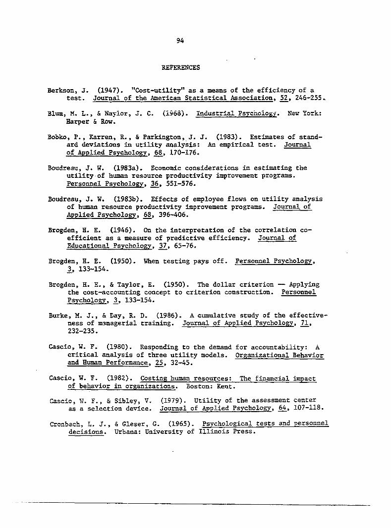
94

REFERENCES

Berkson, J. (1947). "Cost-utility" as a means of the efficiency of a test. Journal of the American Statistical Association, 52, 246-255»

Blum, M, L., & Naylor, J. C. (1966). Industrial Psychology. New York; Harper & Row.

Bobko, P., Karren, R., & Parkington, J. J. (1983). Estimates of stand­ard deviations in utility analysis: An empirical test. Journal of Applied Psychology, 68, 170-176.

Boudreau, J. W. (1983a). Economic considerations in estimating the utility of human resource productivity improvement programs. Personnel Psychology, 36, 551-576.

Boudreau, J. W. (1983b). Effects of employee flows on utility analysis of human resource productivity improvement programs. Journal of Applied Psychology, 68, 396-406.

Brogden, H. E. (1946). On the interpretation of the correlation co­efficient as a measure of predictive efficiency. Journal of Educational Psychology, 37, 65-76.

Brogden, H. E. (1950). When testing pays off. Personnel Psychology, 3, 133-154.

Brogden, H. E., & Taylor, E. (1950). The dollar criterion — Applying the cost-accounting concept to criterion construction. Personnel Psychology, 133-154.

Burke, M. J., & Day, R. D. (1986). A cumulative study of the effective­ness of managerial training. Journal of Applied Psychology, 71, 232-235.

Cascio, W. F. (1980). Responding to the demand for accountability: A critical analysis of three utility models. Organizational Behavior and Human Performance, 25, 32-45.

Cascio, ¥. F. (1982). Costing human resources: The financial impact of behavior in organizations. Boston: Kent.

Cascio, W. F., & Sibley, V. (1979). Utility of the assessment center as a selection device. Journal of Applied Psychology, 64, 107-118.

Cronbach, L. J., & Gleser, G. (1965). Psychological tests and personnel decisions. Urbana: University of Illinois Press.

95

Curtis, E. W., & Alf, E. F. (1969). Validity, predictive efficiency, and practical significance of selection tests. Journal of Applied Psychology. 53, 327-337.

Ford, J. E. (1984). Application of a personalized system of instruction to a large, personnel training program. Improving Staff Effective­ness in Service Settings, 1, 33-46.

Goldstein, I. L. (1980). Training in work organizations. Annual Review of Psychology, 31, 226-260.

Hull, C. L. (1928). Aptitude testing. New York: Harcourt.

Kelley, T. L. (1923). Statistical method. New York; Macmillan.

Kirkpatrick, D. L. (1976). Evaluation of training. In R. L. Craig (Ed.), Training and Development Handbook. New York: McGraw-Hill.

Landy, F. J., & Farr, J. L. (1983). The measurement of work per­formance . New York: Academic Press, Inc.

Landy, F. J., Farr, J. L., & Jacobs, R. R. (1982). Utility concepts in performance measurement. Organizational Behavior and H'™aTi Performance, 30, 15-40.

Lee, R., & Booth, J. M. (1974). A utility analysis of a weighted appli­cation blank designed to predict turnover for clerical employees. Journal of Applied Psychology, 59, 516-518.

Lehman, E. L. (1975). Nonparametrics. Oakland : Holden-Day, Inc.

Mendenhall, E. L. (1983). Nonparametrics; Statistical methods based on ranks. Oakland, CA: Holden-Day, Incorporated.

Munsterberg, H. (1914). Psychology; General and applied. New York; Appleton & Co.

Naylor, J. C., & Shine, L. C. (1965). A table for determining the in­crease in mean criterion score obtained by using a selection device. Journal of Industrial Psychology, 2» 33-42.

Nisbett, R. E., & Wilson, T. D. (1977). Telling morethan we can know: Verbal reports on mental processes. Psychological Review, 84, 231-259.

Sands, W. A. (1973). A method of evaluating alternative recruiting-selection strategies: The CAPER model. Journal of Applied Psy­chology, 57, 222-227.

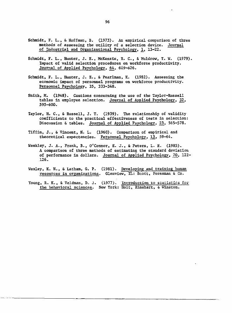
96

Schmidt, F. L., & Hoffman, B. (1973). An empirical comparison of three methods of assessing the utility of a selection device. Journal of Industrial and Organizational Psychology, 13-22.

Schmidt, F. L., Hunter, J. E., McKenzie, R. C., & Muldrow, T. W. (1979). Inçact of valid selection procedures on workforce productivity. Journal of Applied Psychology, 64, 609-626.

Schmidt, F. L., Hunter, J. E., & Pearlman, K. (1982). Assessing the economic intact of personnel programs on workforce productivity. Personnel Psychology, 35, 333-348.

Smith, M. (1948). Cautions concerning the use of the Taylor-Russell tables in employee selection. Journal of Applied Psychology, 32, 595-600.

Taylor, H. C., & Russell, J. T. (1939). The relationship of validity coefficients to the practical effectiveness of tests in selection; Discussion & tables. Journal of Applied Psychology, 23, 565-578.

Tiffin, J., & Vincent, N. L. (1960). Comparison of empirical and theoretical expectancies. Personnel Psychology, 13, 59-64.

Weekley, J. A., Frank, B., O'Connor, E. J., & Peters, L. H. (1985). A comparison of three methods of estimating the standard deviation of performance in dollars. Journal of Applied Psychology, 70, 122-126.

Wexley, K. N., & Latham, G. P. (1981). Developing and training human resources in organizations. Glenvlew, IL: Scott, Foresman & Co.

Young, R. K., & Veldman, D. J. (1977). Introduction to statistics for the behavioral sciences. New York: Holt, Rinehart, & Winston.

97

ACKNOWLEDGMENTS

I wish to thank the members of my committee for their help and en­

couragement (aid and abetment): Drs. Wilbur L. Layton, J. Peter Matilla,

Gary D. Phye, and Robert F. Strahan. A special note of appreciation is

extended to Dr. Kenneth J. Koehler, whose interest and patience were in­

valuable. Most importantly, I am indebted to my major professor. Dr.

Paul M. Muchinsky, for his unfailing guidance and support. Sis high

expectations for graduate scholarship and his quiet confidence in my

ability have helped me to earn a degree in which I have great pride.

Finally, I wish to thank my husband, Kevin Karl Anderson, for his

technical assistance, and my mother, Nellis McMahon Bednarek. Their

love and support has meant more to me than words can express.

This work is respectfully dedicated to my late father,

Casimar Joseph Bednarek 1925-1964