1

COSMOthermX

A Graphical User Interface to the COSMOtherm Program

Tutorial

COSMOlogic GmbH & Co. KG Burscheider Str. 515, D-51381 Leverkusen, Germany

Phone +49-2171-731-683 Fax +49-2171-731-689

E-mail cosmotherm@cosmologic.deWeb http://www.cosmologic.de

2

Introduction: COSMO-RS Theory COSMO-RS is a predictive method for thermodynamic equilibria of fluids and liquid mixtures that uses a statistical thermodynamics approach based on the results of quantum chemical calculations. The underlying quantum chemical model, the so called “COnductor-like Screening MOdel” (COSMO)1, is an efficient variant of dielectric continuum solvation methods. In these calculations the solute molecules are calculated in a virtual conductor environment. In such an environment the solute molecule induces a polarization charge density σ on the interface between the molecule and the conductor, i.e. on the molecular surface. These charges act back on the solute and generate a more polarized electron density than in vacuum. During the quantum chemical self-consistency algorithm, the solute molecule is thus converged to its energetically optimal state in a conductor with respect to electron density. The molecular geometry can be optimized using conventional methods for calculations in vacuum. The quantum chemical calculation has to be performed once for each molecule of interest. The polarization charge density of the COSMO calculation, which is a good local descriptor of the molecular surface polarity, is used to extent the model towards “Real Solvents” (COSMO-RS)2,3. The (3D) polarization density distribution on the surface of each molecule i is converted into a distribution-function, the so called σ-profile pi(σ), which gives the relative amount of surface with polarity σ on the surface of the molecule. The σ-profile for the entire solvent of interest S, which might be a mixture of several compounds, pS(σ) can be built by adding the pi(σ) of the components weighted by their mole fraction xi in the mixture.

( ) ( )∑∈

σ=σSi

iiS pxp (1)

+-

++σ-σ’

HO

H

HO

H OC

O

HO

HHO

H

HO

H

HO

OH H

O

HO

H

Hσ’<<0σ>>0

HO

H

HO

H OC

O

HO

HHO

H

HO

H

HO

OH H

O

HO

H

H

The most important molecular interaction energy modes, i.e. electrostatics (Emisfit) and hydrogen bonding (EHB) are described as functions of the polarization charges of two interacting surface segments σ and σ' or σacceptor and σdonor , if the segments are located on a hydrogen bond donor or acceptor atom. Electrostatic energy arises from the misfit of screening charge densities σ and σ', as

illustrated above. The less specific van der Waal t in a slightly more approximate way.

s (EvdW) interactions are taken into accoun

2)'(2'

)',( σ+σα

=σσ effmisfit aE (2)

( ) ( )( )HBacceptorHBdonorHBeffHB ;;;caE σσσ+σ= 0max0min0min (3)

3

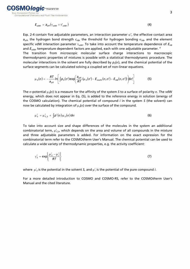
( vdWvdWeffvdW aE 'τ )+τ= (4)

Eqs. 2-4 contain five adjustable parameters, an interaction parameter α’, the effective contact area aeff, the hydrogen bond strength cHB, the threshold for hydrogen bonding σHB, and the element

specific vdW interaction parameter τvdW. To take into account the temperature dependence of EHB and EvdW, temperature dependent factors are applied, each with one adjustable parameter. 4 The transition from microscopic molecular surface charge interactions to macroscopic thermodynamic properties of mixtures is possible with a statistical thermodynamic procedure. The molecular interactions in the solvent are fully described by pS(σ), and the chemical potential of the surface segments can be calculated solving a coupled set of non-linear equations.

( ) ( ) ( ) ( ) ( )( ) ⎥⎦

⎤⎢⎣

⎡σ⎟⎟

⎠

⎞⎜⎜⎝

⎛σσ−σσ−σµσ−=σµ ∫ 'd',','exp'ln HBmisfitS

effS

effS EE

RT

ap

aRT

(5)

The σ-potential µS(σ) is a measure for the affinity of the system S to a surface of polarity σ. The vdW energy, which does not appear in Eq. (5), is added to the reference energy in solution (energy of the COSMO calculation). The chemical potential of compound i in the system S (the solvent) can now be calculated by integration of µS(σ) over the surface of the compound.

( ) ( ) σσµ⋅σ+µ=µ ∫ d , Sii

SCiS p (6)

To take into account size and shape differences of the molecules in the system an additional combinatorial term, µi

C,S, which depends on the area and volume of all compounds in the mixture and three adjustable parameters is added. For information on the exact expression for the combinatorial term refer to the COSMOtherm User’s Manual. The chemical potential can be used to calculate a wide variety of thermodynamic properties, e.g. the activity coefficient:

⎪⎭

⎪⎬⎫

⎪⎩

⎪⎨⎧ µ−µ

=γRT

ii

iSi

S exp (7)

where µi

S is the potential in the solvent S, and µii is the potential of the pure compound i.

For a more detailed introduction to COSMO and COSMO-RS, refer to the COSMOtherm User’s Manual and the cited literature.

4

COSMOtherm and COSMOthermX

COSMOtherm is a command line/file driven program which can be run directly from a UNIX or DOS shell. It allows for the calculation of any solvent or solvent mixture and solute or solute system at variable temperature and pressure. COSMOtherm uses the chemical potentials derived from COSMO-RS theory to compute all kinds of equilibrium thermodynamic properties:

• Vapor pressure, heat of vaporization. • Free energy of solvation, relative stability in solvents. • Activity coefficients, partition coefficients. • Solubility and solid-liquid equilibria (SLE). • Liquid-liquid equilibrium (LLE) and liquid-vapor equilibrium (VLE) phase diagrams (including

azeotropes, miscibility gaps, excess enthalpies and excess free energies). • pKA of acids and bases.

COSMOthermX is a Graphical User Interface to the COSMOtherm command line program. It allows for the interactive use of the COSMOtherm program, i.e. selection of compounds, preparation of property input, program runs and display of calculation results.

Getting Started

At initial start of COSMOthermX a dialog opens where some settings are already specified: Paths for the COSMOtherm executable and the CTDATA directory of the COSMOtherm installation are set, and the parameter files for the quantum chemical levels (extension .ctd) are specified. Additionally, you can set paths for the Adobe Acrobat Reader and a browser. The Adobe Acrobat Reader path is required to view the COSMOtherm User’s Manual and this tutorial directly from the user interface. If you intend to use cosmo-Meta files (extension .mcos) for the fragment approach, you should also specify the fragment directory. The databases that come with the COSMOtherm release are specified in the “Databases” panel. Moreover, additional databases can be added in this panel with “Add Databases”. This opens a dialog where you can enter the database name and the database directory. Select the parameterization which matches the quantum chemical level of the database. For detailed information on adding your own databases, refer to the section “Using your own COSMO files”. The settings can always be changed in the “Run” menu under “Settings”. Changes can be done for the current session only, e.g. in order to use a special parameterization for the current session only, or permanently.

5

Quality levels and Parameterizations

The input for the compounds is read from the COSMO files, identified by the extensions .cosmo or .ccf, which are result files from quantum chemical COSMO calculations. At least one COSMO file has to be selected as compound input. COSMOtherm extracts the relevant information directly from the COSMO files. The compressed COSMO files (.ccf) use significantly less disk space than conventional COSMO files. COSMO files shipped with COSMOtherm are available on two quantum chemical levels. The application of COSMOtherm in chemical and engineering thermodynamics (e.g. prediction of binary VLE or LLE data, activity coefficients in solution or vapor pressures) typically requires high quality of property predictions of mixtures of small to medium sized molecules (up to 25 non-Hydrogen atoms). The recommended quantum chemical method for such a problem is a full Turbomole BP-RI-DFT COSMO optimization of the molecular structure using the large TZVP basis set5, in the following denoted BP-TZVP. Screening a large number of compounds, e.g. prediction of solubility of compounds in various solvents, typically requires a predictive quality that is somewhat lower than for chemical engineering applications. The molecules involved are often larger (>100 atoms) and an overall large number of compounds has to be computed by quantum chemistry. Thus a compromise between computational demands and quality of the predictions has to be made: A very good compromise is the optimization of molecular geometry on the computationally very cheap semiempirical MOPAC AM1-COSMO level6 with a subsequent single point COSMO calculation on Turbomole BP-RI-DFT COSMO level using the small SVP basis set. This method is named BP-SVP-AM1 in the following. Because the quality, accuracy, and systematic errors of the electrostatics resulting from the underlying quantum chemical COSMO calculations depend on the quantum chemical method as well as on the basis set, COSMOtherm needs a special parameterization for each of these method / basis set combinations. The BP_TZVP_C21_0107.ctd parameter file should be used with COSMO files from BP-TZVP COSMO calculations, while the BP_SVP_AM1_C21_0107.ctd parameter file should be used with COSMO files from BP-SVP-AM1 calculations. For information on other available quantum chemical levels and parameterizations refer to the COSMOtherm User’s Manual, section 3.

General

The COSMOthermX main window has several menus:

• File: o New: Create a new input file. Type the filename and press “Open”. Also available as

shortcut . o Open: Open an existing input file. Select a file from the directory or type the filename

into the “File name” text field and press “Open”. The panel also allows for changing

the directory. Also available as shortcut . o Save: Save the input file to the current directory with the actual name. Also available as

shortcut . o Save As…: Choose a directory and a name for the input file to be saved.

6

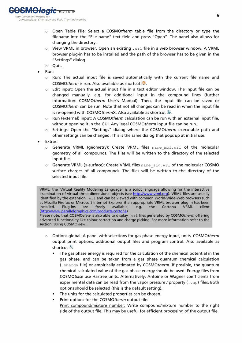
o Open Table File: Select a COSMOtherm table file from the directory or type the filename into the “File name” text field and press “Open”. The panel also allows for changing the directory.

o View VRML in browser. Open an existing .wrl file in a web browser window. A VRML browser plug-in has to be installed and the path of the browser has to be given in the “Settings” dialog.

o Quit. • Run:

o Run: The actual input file is saved automatically with the current file name and

COSMOtherm is run. Also available as shortcut . o Edit input: Open the actual input file in a text editor window. The input file can be

changed manually, e.g. for additional input in the compound lines (further information: COSMOtherm User’s Manual). Then, the input file can be saved or COSMOtherm can be run. Note that not all changes can be read in when the input file

is re-opened with COSMOthermX. Also available as shortcut . o Run (external) input: A COSMOtherm calculation can be run with an external input file,

without opening it in the GUI. Any legal COSMOtherm input file can be run. o Settings: Open the “Settings” dialog where the COSMOtherm executable path and

other settings can be changed. This is the same dialog that pops up at initial use. • Extras:

o Generate VRML (geometry): Create VRML files name_mol.wrl of the molecular geometry of all compounds. The files will be written to the directory of the selected input file.

o Generate VRML (σ-surface): Create VRML files name_sig.wrl of the molecular COSMO surface charges of all compounds. The files will be written to the directory of the selected input file.

VRML, the ‘Virtual Reality Modeling Language’, is a script language allowing for the interactiveexamination of virtual three-dimensional objects (see http://www.vrml.org). VRML files are usuallyidentified by the extension .wrl and can be viewed with common World-Wide-Web browsers suchas Mozilla Firefox or Microsoft Internet Explorer if an appropriate VRML browser plug in has beeninstalled. Plug-ins are freely available, e.g. the Cortona VRML client(http://www.parallelgraphics.com/products/cortona) Please note, that COSMOview is also able to display .wrl files generated by COSMOtherm offeringadvanced functionality like colour correction and charge picking. For more information refer to thesection 'Using COSMOview'.

o Options global: A panel with selections for gas phase energy input, units, COSMOtherm output print options, additional output files and program control. Also available as

shortcut . The gas phase energy is required for the calculation of the chemical potential in the

gas phase, and can be taken from a gas phase quantum chemical calculation (.energy file) or empirically estimated by COSMOtherm. If possible, the quantum chemical calculated value of the gas phase energy should be used. Energy files from COSMObase use Hartree units. Alternatively, Antoine or Wagner coefficients from experimental data can be read from the vapor pressure / property (.vap) files. Both options should be selected (this is the default setting).

The units for the calculated properties can be chosen. Print options for the COSMOtherm output file:

Print compound/mixture number: Write compound/mixture number to the right side of the output file. This may be useful for efficient processing of the output file.

7

Print conformer info: If a compound input consists of several conformers this option causes the output of the calculated COSMOtherm mixture information to be written for each individual conformer. By default, only the results for the mixed compound are written to the output file.

Suppress pure compounds info: Do not write the pure compound information to the output file.

Suppress mixture output in .out file: Do not write the mixture information to the output file.

Print 15 digit long numbers to .out-file: Print all real numbers in scientific exponent number format with 15 significant digits to the output file.

Print full length atomic weight string: Print complete atomic weight or real weight string to the compound section of the output file. If you toggle this option, the file line for the atomic weights may become very long.

Print molecular surface contacts: Print statistics of molecular surface contacts for all compounds in all mixtures to the output file. For a detailed description see section 5.7 of the COSMOtherm User’s Manual.

Print detailed segment molecule contacts: Print statistics of the molecular surface contacts for all segments of all compounds in all mixtures to the output file to the contact statistics table file name.contact. Refer to the COSMOtherm User’s Manual, section 5.7, for details.

Print derivatives of chemical potential: Print the values of the temperature and composition derivatives of the chemical potentials of all compounds in all mixtures to the output file. See section 5.6 “Chemical Potential Gradients” of the COSMOtherm User’s Manual for further information.

Additional output files: σ-moments (.mom): Write the σ-moments of all processed compounds in tabulated

form to filename.mom. In addition some other molecular information will be written to filename.mom, including volume V, molecular weight, dielectric energy Ediel, average energy correction dE, van der Waals energy in continuum Evdw, ring correction energy Ering and the standard chemical potential of the molecule in the gas phase with respect to the ideally screened state µgas = ECOSMO - Egas + dE + EvdW + Ering – ηgasRT, using T = 25°C. Refer also to sections 5.4 and 5.5 of the COSMOtherm User’s Manual.

Atomic σ-moments (.moma): Write the atomic σ-moments of all processed

compounds to filename.moma. If this option is used, σ-moments will be calculated for each atom of the compounds.

σ-Profiles (.prf): Write the σ-profiles of all processed compounds to file

filename.prf. A summary of the σ-profiles will be written in tabulated form to the table file filename.tab.

σ-Potentials (.pot): Write the σ-potentials of all calculated mixtures to

filename.pot. A summary of the σ-potential information will be written in tabulated form to the table file filename.tab.

Program control settings: Switch off temp. dependency of hydrogen bond contrib.: Switch off temperature

dependency of the hydrogen bond contribution to the total interaction energy of the compound for the complete COSMOtherm run.

Switch off temp. dependency of van der Waals contrib.: Switch off temperature dependency of the van der Waals contribution to the total interaction energy of the compound, active for the complete COSMOtherm run.

8

Switch off combinatorial contrib. to chemical potential: Switch off combinatorial contribution to the chemical potential for the complete COSMOtherm run.

Change threshold for the iterative self-consistency: Change threshold for the iterative self-consistency cycle for the determination of the chemical potential. A smaller value leads to higher accuracy of the COSMOtherm results but also to a longer computational time due to an increasing number of iterations. Default value: 10-8.

MDIR path settings: Set the directory where to search for the .cosmo or .ccf files referenced in the COSMO-metafiles (.mcos). “Fragment directory” sets the mdir path to the Fragment directory indicated in the “Settings” dialog. “local” sets the mdir path to be identical to the fdir path of the .mcos file.

o Mixture Options: A panel with options applying to settings for the mixture calculation.

Also available as shortcut Mixture Options. Settings from the mixture options dialog allow for fundamental changes in the mixture calculaton. Note that mixture options will only be used if the “Use Mixture Options” checkbox is activated in the property panel. If several mixtures or properties are calculated in a single run, the mixture options have to be activated each time the property settings are transferred the property selection window, otherwise they will not be used for the respective property calculation. Print options for the COSMOtherm output file:

Suppress mixture output in .out-file: Do not write the mixture information to the output file.

Select compounds printed in .out file: Write to the COSMOtherm output file the evaluated information only for the selected compounds. Helps to shorten the output file if not all evaluated information is required by the user.

Program control settings: Print derivatives of chemical potential: Print the values of the temperature and

composition derivatives of the chemical potentials of all compounds in all mixtures to the output file. See COSMOtherm User’s Manual, section 5.6 “Chemical Potential Gradients” for further information.

Switch off temp. dependency of hydrogen bond contrib.: Switch off temperature dependency of the hydrogen bond contribution to the total interaction energy of the compound for the complete COSMOtherm run.

Switch off temp. dependency of van der Waals contrib.: Switch off temperature dependency of the van der Waals contribution to the total interaction energy of the compound, active for the complete COSMOtherm run.

Switch of hydrogen bonding: Switch off hydrogen bonding (HB) contribution to the chemical potential.

Switch off van der Waals contributions: Switch off van der Waals (vdW) interaction energy contribution to the chemical potential.

Switch off combinatorial contrib. to chemical potential: Switch off combinatorial contribution to the chemical potential for the complete COSMOtherm run.

Do not check for charge neutrality: Overrides the check for charge neutrality of a given mixture composition and allows you to compute non-neutral mixtures.

Advanced Settings: Switch of combinatorial contribution for specific compounds: The combinatorial contribution is switched off for the selected compounds only.

• QSPR: A menu with the options logPOW, logBB, logKOC, logKIA, logKHSA. These options

enable a calculation of the chosen property with the provided QSPR parameterization. Since the parameterization is on the BP-SVP-AM1 level, compounds have to be chosen from

9

the SVP Database. Currently, there can always only one property be chosen. For the calculation of several QSPR properties in a single run please refer to the COSMOtherm User’s Manual. By default, the computed property value will be listed in the compound section of the COSMOtherm output file. An additional file with the extension .mom will be

written, listing the molecular σ-moments and, in the last column, the computed property. Note that QSPR property calculations can also be done from the Mix-QSPR card, which allows for a larger variety of settings.

• Tools: o VRML-Viewer: Opens the COSMOview tool which allows for the visualization of .wrl

files generated by COSMOtherm. For more information, please refer to the section “Using COSMOview”.

o mcos-File Editor: Opens the COSMOweight tool. For information on atom weighting and the COSMOweight tool, please refer to the section “Atom Weighting”.

• Help: o Physical Constants: Information about some physical constants and conversion factors

and some parameters is displayed. o COSMOtherm Manual: Open the COSMOtherm User’s Manual with the Adobe Acrobat

Reader. The Adobe Acrobat executable path has to be set correctly in the “Run”-“Settings” dialog.

o COSMOthermX Tutorial: Open the COSMOthermX Tutorial (this document) with the Adobe Acrobat Reader. The Adobe Acrobat executable path has to be set correctly in the “Run”-“Settings” dialog.

Apart from the menu and shortcut bars, the COSMOthermX main window has two sections. The section on the left side contains a window listing the selected compounds. At the bottom of this section, there are buttons to open the File Manager or database files from which the compounds can be selected.

• File Manager: Opens the directory tree of your system and enables to choose COSMO files of any quantum chemical level directly from the file system. If you do not plan to use any compounds other than those provided with your COSMOtherm installation, it is more convenient to use the Database buttons.

• TZVP Database: Opens the TZVP Database index files in tabulated form. The location of the database index file from the COSMOtherm release is set automatically. Locations for other databases have to be given in the “Databases” panel of the “Settings” dialog. For detailed information on the use of your own databases, refer to the section “Using your own COSMO files”.

• SVP-Database: Same as TZVP-Database, but compounds are calculated on the BP-SVP-AM1 quantum chemical level.

• Clear: Clear all compounds from the selection window. (Individual compounds can be removed using the Delete key.)

• Activate Conformers Treatment: If this check-box is marked and you have selected more than one conformer for a compound, the conformers will be weighted internally by COSMOtherm using their COSMO energy and their chemical potential. For more information on conformer input refer to the COSMOtherm User’s Manual, section 2.2.2. If you intend to use your own COSMO files for conformers please be aware that the names of

10

the files must follow a convention in order to be identified as conformers by COSMOthermX.

Databases of one level are available from panels in the database window. The database tables can be sorted with respect to number, COSMO-name (which is the name of the .cosmo or .ccf file), CAS-Number, Molecular Weight, and Formula. For some compounds, there are several conformers

with different σ-profiles to be considered. By default, all available conformers are selected. You can uncheck the selection to use only the lowest energy conformer. In case you should need a specific conformer other than the lowest energy conformer, you can use the “Del” key to delete the unwanted conformers from the selection or select it from the File Manager. The database tables can also be searched for compounds. It is possible to enter a search string or open a text file with a list of compound names which will then be searched for in the database. Note that the search is processed in the current database only. Inside the File Manager or the database files, a list of compounds can be highlighted by using the “Ctrl” or “Shift” keys together with the mouse. A right mouse button click opens a context menu with several options for the highlighted compound:

11

• Compound Properties: Pure compound property data can be edited. Data entries in the dialog come from the .vap file of the compound. Properties highlighted in green indicate

that data entries are available, while for properties highlighted in blue no data are entered so far. Data can be changed or added and can subsequently be used in the COSMOtherm input for the current calculation only or saved permanently to the .vap file. Note that if applied to database compounds “Save to Vap” will change the corresponding .vap files in the database permanently.

• Open: Opens the .cosmo or .ccf file of the compound in a text editor.

• View molecule: 3D ball-and-stick model of the molecular geometry. • Convert selection: The selected files can be converted into a variety of other file types like

.pdb or .ml2.

• Sigma-surface: 3D preview of the molecular σ-surface. This graphic has a lower resolution

than the graphic you get from a VRML of the σ-surface in a VRML viewer. • Sigma-profiles /-potentials: The σ-profiles and the σ-potentials of the selected compounds

are plotted. • Write to list: The selected files can be written to a list which can be used for further

processing.

• Edit weight string: Opens the .cosmo or .ccf file in the COSMOweight tool. Changes in the weight string will be saved to the input file. Refer to the section “Atom weighting” for information on the use of the COSMOweight tool. Note that this option is only available in the compound list and only if the conformers treatment is deactivated.

• Edit .mcos-File: Opens the .cosmo or .ccf file in the COSMOweight tool and allows for the creation of a .mcos file. Refer to the section “Atom weighting” for information on the use of the COSMOweight tool. Note that this option is only available in the compound list and only if the conformers treatment is deactivated.

The options “View molecule”, “Sigma-surface” and “Sigma-profiles /-potentials” from the context menu require a COSMOtherm run in the background. Output files of the runs are written to

12

temporary files which will be removed when the display windows are closed. For the 3D ball-and-stick model of the molecular geometry or the σ-surface of the molecule to be written to permanent

files check the corresponding check-boxes in the “Extras” menu. σ-profiles and σ-potentials are written to permanent files with the extensions .prf and .pot when the corresponding options in the “Options” dialog are selected. The larger section of the main window offers a selection of property cards. Inside each card you can adjust parameters like temperature, mole fraction etc. to your issue. Input settings from the property cards are transferred to the Property Selection panel with the “Add” button. Changes in the “Mixture Options” dialog are taken into account for the property if the “Use Mixture Options” checkbox is activated. The COSMOtherm calculation is started with “Run” from the “Run” menu or from the shortcut bar. For a detailed description of the different options for properties, refer to the following sections. By default, COSMOtherm produces two sorts of output files for most property calculations: The COSMOtherm output file filename.out and a file filename.tab which contains the calculated property information in tabulated form. These files will automatically pop up in a text editor window after the calculation has finished. In case of a binary mixture calculation the .tab file will be displayed in a graphical viewer application. Additional output files will be written if the corresponding options in the “Extras” menu under “Options” are activated. These output files may

contain σ-moments (.mom), atomic σ-moment (.moma), σ-profiles (.prf), or σ-potentials (.pot).

13

Visualization of σ-surfaces, σ-profiles, and σ-potentials

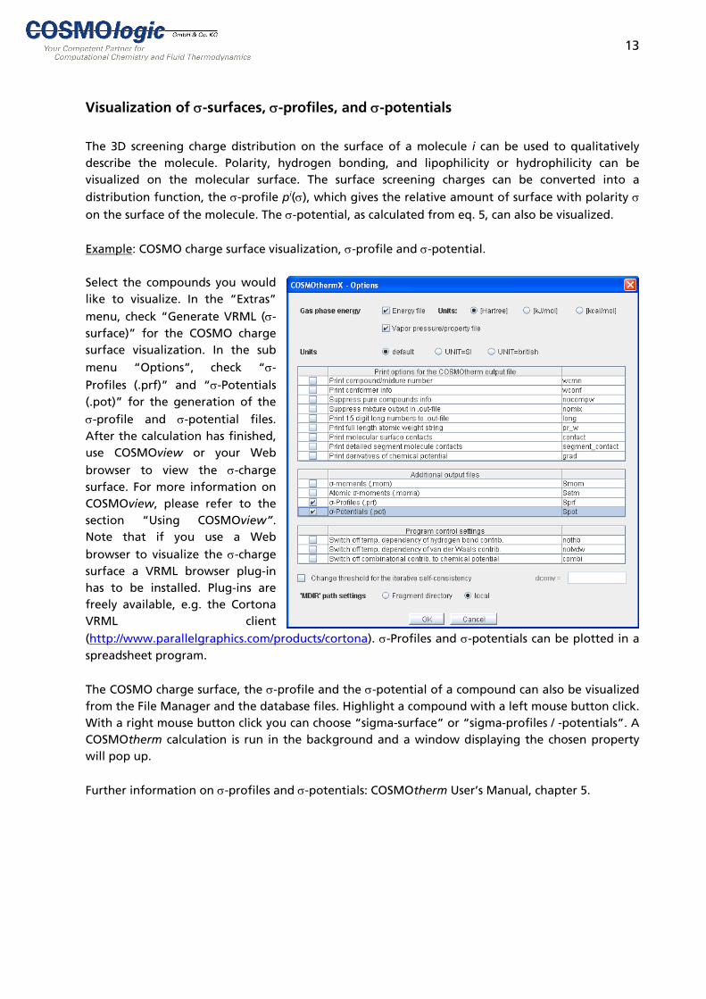
The 3D screening charge distribution on the surface of a molecule i can be used to qualitatively describe the molecule. Polarity, hydrogen bonding, and lipophilicity or hydrophilicity can be visualized on the molecular surface. The surface screening charges can be converted into a distribution function, the σ-profile pi(σ), which gives the relative amount of surface with polarity σ on the surface of the molecule. The σ-potential, as calculated from eq. 5, can also be visualized. Example: COSMO charge surface visualization, σ-profile and σ-potential. Select the compounds you would like to visualize. In the “Extras” menu, check “Generate VRML (σ-surface)” for the COSMO charge surface visualization. In the sub menu “Options”, check “σ-Profiles (.prf)” and “σ-Potentials (.pot)” for the generation of the σ-profile and σ-potential files. After the calculation has finished, use COSMOview or your Web browser to view the σ-charge surface. For more information on COSMOview, please refer to the section “Using COSMOview”. Note that if you use a Web browser to visualize the σ-charge surface a VRML browser plug-in has to be installed. Plug-ins are freely available, e.g. the Cortona VRML client (http://www.parallelgraphics.com/products/cortona). σ-Profiles and σ-potentials can be plotted in a spreadsheet program. The COSMO charge surface, the σ-profile and the σ-potential of a compound can also be visualized from the File Manager and the database files. Highlight a compound with a left mouse button click. With a right mouse button click you can choose “sigma-surface” or “sigma-profiles / -potentials”. A COSMOtherm calculation is run in the background and a window displaying the chosen property will pop up. Further information on σ-profiles and σ-potentials: COSMOtherm User’s Manual, chapter 5.

14

Using COSMOview

Additionally to using third-party web browser plug-ins to display .wrl files generated by COSMOtherm, you can also use COSMOview. COSMOview is included in COSMOthermX and can be accessed via “Tools”-“COSMOview” or by right-clicking a compound and selecting “View sigma surface” or “View molecule”. You will be presented with an empty window or your molecule already loaded, respectively. In the former case open a previously generated VRML file by clicking

the leftmost toolbar button . Movement: Molecules can be moved using the mouse buttons

• Rotate the molecule by dragging the mouse with the left button pressed. If you move the mouse quickly, you can give the molecule a spin to have it turn by itself.

• Zoom in and out with the right mouse button pressed or simply by turning the mouse wheel.

• When examining a very large structure, you may want to focus on a certain region rather

than at its center. Deactivate the “Rotation around origin” button . Now dragging with the left mouse button rotates the “camera”, i.e. your view port around itself, whilst dragging with the right mouse button or turning the mouse wheel moves the camera in the direction it is facing. This offers a broad range of perspectives not accessible by mere rotation.

• Use the "home" button to reset the camera to its initial position. Customizing the visual appearance / Taking images: With the buttons from the toolbar you can

• Set the background color ,

• Show/hide the sigma surface (if loaded) ,

• Show/hide the molecule itself ,

• Toggle wire frame display ,

• Save graphics . Graphics can be saved with transparent background and/or a small legend optionally. Please note that since COSMOview uses an internal color correction, the legend produced will not be applicable to images obtained by other means than COSMOview, e.g. third-party browser plug-ins.

The options for customizing the visualization will especially be handy when you want to save graphics for later use, e.g. for presentations. Charge picking:

• To get an idea of the quantitative surface charge density at a given point, you can activate

the charge picking mode with and move the cursor over the σ-surface. A slider at the right-hand side will display the charge density at the sport you are pointing on. However these values can only be approximated and are not guaranteed to be entirely precise. This is mainly an effect of interpolation between the reduced grid size compared to .cosmo files.

You may want to check the file properties .

Please note that like most 3D-viewers, COSMOview requires OpenGL v1.1. If it does not start up at all (especially in X window environments), make sure that both your display and the X client are glx capable.

15

Text Viewer Options

Some of the output files produced by COSMOtherm can be saved in MS Excel format or (on Windows systems with MS Excel) opened directly in an MS Excel spreadsheet, using the options “Open with MS Excel” or “Save As”. These options are available for .tab, .prf, .pot, and .mom files.

16

Property input In this section, the different options for the calculation of properties are described. There are also examples for some calculations.

Mixture: Calculation of compound properties in mixture

This option toggles the COSMOtherm calculation of interaction energy terms at the given temperature and mixture composition. For all compounds i in the compound list, the following terms will be calculated:

• Chemical potential µSi of the compound in the mixture from eq (6).

• Log10(partial pressure [mbar]) • Free energy of the molecule in the mixture (E_COSMO+dE+Mu) • Total mean interaction energy in the mix (H_int): The mean interaction enthalpy of the

compound with its surrounding, i.e. the interaction enthalpy of the compound which can be used to derive heats of mixing and heats of vaporization.

• Contributions to the total mean interaction energy: o Misfit interaction energy in the mix (H_MF). o H-Bond interaction energy in the mix (H_HB) o VdW interaction energy in the mix (H_vdW) o Ring correction

For details on the calculation of the energy terms and contributions please refer to the COSMOtherm User’s Manual, section 1.1. Furthermore, COSMOtherm allows for the computation of the contact probability of molecules and molecule surface segments in arbitrary mixtures. The checkbox “Compute Contact Statistics” can be checked to obtain a more detailed contact interaction statistics of all segments of molecules A and B. For more information on the calculation of contact statistics please refer to the COSMOtherm User’s Manual, section 5.7.

Vapor Pressure

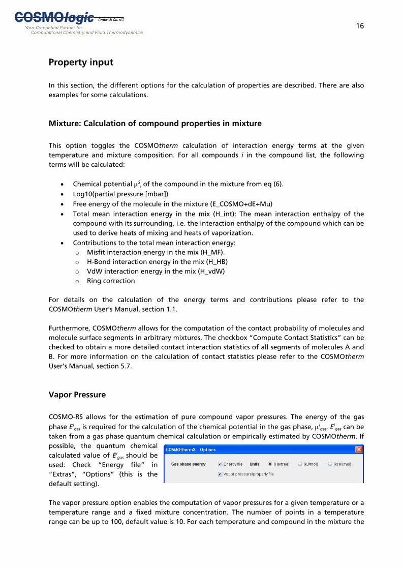
COSMO-RS allows for the estimation of pure compound vapor pressures. The energy of the gas phase Ei

gas is required for the calculation of the chemical potential in the gas phase, µigas. Ei

gas can be taken from a gas phase quantum chemical calculation or empirically estimated by COSMOtherm. If possible, the quantum chemical calculated value of Ei

gas should be used: Check “Energy file” in “Extras”, “Options” (this is the default setting). The vapor pressure option enables the computation of vapor pressures for a given temperature or a temperature range and a fixed mixture concentration. The number of points in a temperature range can be up to 100, default value is 10. For each temperature and compound in the mixture the

17

partial vapor pressures, the chemical potential of the compound in the gas phase and its enthalpy of vaporization are computed and written to the COSMOtherm output file. The total vapor pressure of the mixture is written to the COSMOtherm table file in tabulated form pVAP vs T. In addition the total chemical potentials of the liquid µLIQUID

(tot) and of the gas phase µGAS(tot), as well as

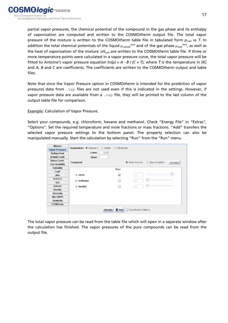
the heat of vaporization of the mixture ∆HVAP are written to the COSMOtherm table file. If three or more temperature points were calculated in a vapor pressure curve, the total vapor pressure will be fitted to Antoine’s vapor pressure equation ln(p) = A - B / (C + T), where T is the temperature in [K] and A, B and C are coefficients. The coefficients are written to the COSMOtherm output and table files. Note that since the Vapor Pressure option in COSMOtherm is intended for the prediction of vapor pressures data from .vap files are not used even if this is indicated in the settings. However, if vapor pressure data are available from a .vap file, they will be printed to the last column of the output table file for comparison. Example: Calculation of Vapor Pressure. Select your compounds, e.g. chloroform, hexane and methanol. Check “Energy File” in “Extras”, “Options”. Set the required temperature and mole fractions or mass fractions. “Add” transfers the selected vapor pressure settings to the bottom panel. The property selection can also be manipulated manually. Start the calculation by selecting “Run” from the “Run” menu.

The total vapor pressure can be read from the table file which will open in a separate window after the calculation has finished. The vapor pressures of the pure compounds can be read from the output file.

18

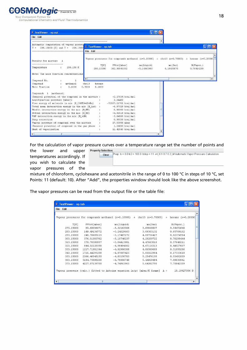
For the calculation of vapor pressure curves over a temperature range set the number of points and the lower and upper temperatures accordingly. If you wish to calculate the vapor pressures of the mixture of chloroform, cyclohexane and acetonitrile in the range of 0 to 100 °C in steps of 10 °C, set Points: 11 (default: 10). After “Add”, the properties window should look like the above screenshot. The vapor pressures can be read from the output file or the table file:

19

Boiling Point

This option enables the iterative optimization of the equilibrium temperature for a given vapor pressure. The temperature of the system is varied and for each temperature the vapor pressure is calculated. This is repeated until the COSMOtherm prediction of the total vapor pressure and the specified pressure in the input file is below a certain threshold. During the procedure, the partial vapor pressures of the compounds are written to the COSMOtherm output file. When the required threshold is met, i.e. convergence is reached, the total vapor pressure of the mixture is written to the COSMOtherm table file.

Activity Coefficient Calculation

This option computes the activity coefficients of different compounds in the selected solvent or solvent mixture. For the calculation of the activity coefficient at infinite dilution, the mole or mass fraction of the compound of interest has to be set to zero in the composition of the solution. The chemical potentials µj

(P) of all pure compounds j and the chemical potentials µj(i) in the liquid phase

(compound i or compound mixture, respectively) are calculated. The activity coefficients are then calculated as ln(γj) = (µj

(i) – µj(P)) / RT.

It is also possible to calculate the activity coefficients at a given finite concentration. This is achieved by setting the mole or mass fraction of the compound of interest to the required value in the composition of the solvent. The compound in question is thus treated as part of the solvent. Example: Calculate the activity coefficient of aspirin in water. Choose the compounds from the database files or the File Manager. By default, both aspirin conformers are selected from the database and the conformer treatment is activated to account for a conformer mixture. Then, set the temperature to the desired value, set the water mole fraction to 1.0 (check “pure”), and transfer the selection to the property panel with the “Add” button.

Windows displaying the output and table files will open after the calculation has finished.

20

Henry Law Coefficient Calculation

This option allows for the computation of Henry law coefficients H(i) in compound i. The chemical potentials µj

(P) of all pure compounds j and the chemical potentials µj(i) at infinite dilution in

compound i are calculated. Then the Henry law coefficients Hj(i) for all compounds j are calculated

from the activity coefficients and the vapor pressures of the compounds are written to the COSMOtherm output and table files. It is also possible to calculate the Henry law coefficients at a given finite concentration, i.e. in a mixture of solvents. The Henry law coefficient depends on the pure compound vapor pressure. For each compound, there are several possibilities to calculate or approximate this property. In order of increasing accuracy you might:

• Use the COSMOtherm approximation of the vapor pressure using the approximated gas phase energy of the compound. This is the default and requires no additional input.

• Use the COSMOtherm approximation of the vapor pressure using the exact gas phase energy of the compound from the .energy file. This option is set by default. (“Extras”, “Options”: Check “Energy file”)

• Use the Wagner, DIPPR, or Antoine equation ln(pj0) = A – B / (T + C) to compute the vapor

pressure at the given temperature. If available, data for these equations will be read from the .vap file if the “Vapor pressure / property file” option is checked in the “Options” dialog. Data can also be entered in the “compound properties” dialog from the right mouse button menu for the compound.

• Enter the exact value of the vapor pressure for this temperature via the “compound properties” dialog.

Gas Solubility

With this option the solubility of a gas in a solvent or solvent mixture can be calculated in an iterative procedure. For each compound j the mole fraction xj is varied until the partial pressure of the compound pj = pj

0 xj γj (with the activity coefficient γj and the pure compound vapor pressure pj0)

is equal to the given reference pressure p. Like the calculation of the Henry Law Coefficient, the calculation of a gas solubility requires the knowledge of the pure compound vapor pressure. For options to give the pure compound vapor pressure please refer to the Henry Law Coefficient Calculation section. Example: Gas solubility of methane in water

21

Select the compounds, water and methane, from the TZVP database. Set the temperature and the pressure in the Gas-Solubility card. Set the solvent composition to pure water. Transfer the settings to the “Property Selection” by pressing “Add” and run the program.

Windows displaying the output and table files will open after the calculation has finished.

Solubility

The Solubility option allows for the automatic computation of the solubility of liquid or solid compounds in a solvent i. The chemical potentials µj

(P) of all pure compounds j, the chemical potentials µj

(H2O) of all compounds in water and the chemical potentials µj(i) at infinite dilution in

compound i are calculated. The computed solubility x(0)sol is a zeroth order approximation, which is

valid only for small concentrations of the solute. If the solubility is large (xsol > 0.1), x(0)sol is a poor

approximation, but xsol can be refined iteratively by resubstitution of x(0)sol into the solubility

calculation. This procedure can be repeated until the differences in the computed value of xsol are below a certain threshold. In COSMOthermX, this procedure is turned on by checking the “Iterative” calculation type in the Solubility card. COSMOtherm is able to calculate compounds in the liquid phase only. For the solubility of solid compounds the Gibbs free energy ∆Gfus has to be taken into account. ∆Gfus can be read from the vapor pressure / property file or from the compound line in the compound input section of the COSMOtherm input file. A temperature dependent heat of fusion can also be calculated if the compounds enthalpy or entropy of fusion (∆Hfus or ∆Sfus) and melting temperature are known. To add ∆Gfus (or ∆Hfus or ∆Sfus and Tmelt) to the compound input lines open the “compound properties”

dialog for the compound. Alternatively, ∆Gfus can be estimated by COSMOtherm using a QSPR approach. QSPR parameters are read from the parameter file, if possible, but can also be given explicitly in the COSMOtherm input file. Since one of the QSPR parameters is the chemical potential of the compound in water, water has to be included in the compound list even if it is not present in the sytem. For further information refer to the COSMOtherm User’s Manual, section 2.3.4. The output of the solubility option is in logarithmic mole fractions, log10(x). To calculate the solubility in the more commonly used g/L units, the molecular weights and the solvent density have to be known. Example: See VLE / LLE

22

Partition Coefficient Calculation (Log P)

Partition coefficients of solute j between solvents i1 und i2 are defined as P1,2 = cj

1 / cj2, with cj

1 and cj2

being the concentrations of solute j in i1 and i2, respectively. The calculation of the partition coefficient logP is accomplished via computation of the chemical potentials µj

(1) and µj(2) of all

compounds j in infinite dilution in pure compounds i1 and i2, respectively:

(8) ]/)/)[exp((log)(log 21)2()1(

1010 VVRTP jj ⋅µ−µ=

The volume quotient V1/V2 will be estimated from the COSMO volumes by default, unless a volume quotient value is entered in the Log P card. The input of a volume quotient will be necessary if the densities of the two solvent phases differ substantially and thus the estimate from the COSMO volumes, based on the assumption of an incompressible liquid, will be poor. Furthermore, the mutual solubility of the solvents in each other has to be taken into account when computing µj

(1) and µj

(2). It is possible to give finite concentrations in the solvent mixture section. Example: Prediction of Octanol / Water partition coefficients. Select your compounds, e.g. water, 1-octanol and caffeine from the database file or the File Manager. In the Log P card, set the temperature and the value for the volume quotient (0.11415 for Phase 1: water, Phase 2: octanol). Then set the solvent concentrations for the two phases:

The “wet octanol” phase contains 0.24 mole fractions of water. Finally, add your settings to the property panel (“Add”) and run the program. The partition coefficients can be read from the output and table files. In the table file, the results are listed:

23

Calculation of pKA

The pKA of a solute j can be estimated from the linear free energy relationship (LFER),

(9) )(pK 10Ajion

jneutral GGcc ∆−∆+=

where ∆Gj are the free energies of the neutral and the ionic compounds. The pKA option allows for the computation of the pKA value of a compound in a solvent i (usually water). The free energies ∆Gj in the solvent at infinite dilution are computed and the pKA is estimated from the above LFER. Thus, to obtain a pKA value it is necessary to do quantum chemical COSMO calculations of a molecule in its neutral and in its ionic state. Since the LFER is valid for both anions and cations it is possible to estimate acidity as well as basicity. The LFER parameters c0 and c1 are read from the COSMOtherm parameter file by default. pKA prediction by COSMOtherm is not restrictd to aqueous acid pKA. However, both aqueous base pKA prediction and pKA in solvents other than water require reparameterization of the pKA LFER parameters. LFER parameters for aqueous base pKA, pKA in solvents dimethylsulfoxide (DMSO) and acetonitrile at room temperature are shipped within the COSMOtherm parameter files BP_TZVP_C21_0107.ctd and BP_SVP_AM1_C21_0107.ctd. The parameterizations will be used by COSMOtherm if the corresponding options are selected from the pKA card. Note that the solvent has to be set corresponding to the selected option for the LFER parameters. LFER parameters for solvent-solute systems other than those provided by COSMOtherm or for temperatures other than room temperature can be set by selecting the “Advanced Settings” check-box to enter the LFER parameters. Note that for secondary and tertiary aliphatic amines COSMOtherm systematically underestimates the base pKA. This underestimation is the result of a well known problem of continuum solvation models like COSMO with aliphatic amines and amino-cations in polar solvents. The error is systematic and can be accounted for by a simple correction term. Refer to the COSMOtherm User’s Manual, section 2.3.6 for directions. For the computation of higher states of ionization, the neutral and singly charged ionic species have to be replaced by higher ionized species.

24

Example: Calculation of the aqeous pKA of 4-chlorophenol. Select the solvent (water), and the neutral and ionic compounds (4-chlorophenol and 4-chlorophenol-anion), with the File Manager or from the databases. Set the temperature, and make sure to use water as the solvent. Set the neutral and ionic compounds from the menus. Select “Water-Acid” as parameters for the Solvent-Solute system and add the settings to the property panel with “Add”. Note that it is possible to reset the compounds and also add them to the input. In that case, COSMOtherm will do more than one property calculation and write the results to the output and table files. Since we have chosen room temperature and water as solvent for the calculation, no further settings are necessary. If you want to use your own LFER parameters, input is possible via the “Advanced Settings” option. Save the input file and run the calculation. The COSMOtherm output and table files will open after the calculation has finished.

The table file lists the computed pKAs:

25

Vapor-Liquid Equilibria (VLE) and Liquid-Liquid Equilibria (LLE)

COSMOtherm allows for the computation of phase diagrams (VLE and LLE) of binary, ternary or higher dimensional (multinary) mixtures. It is possible to calculate phase diagrams at fixed pressure (isobaric) or at fixed temperature (isothermal). The pressure or temperature has to be given in the input. The program automatically computes a list of concentrations covering the whole range of mole fractions of the binary, ternary or multinary mixture. Then,

• the excess properties HE and GE, • the activity coefficient γi, • the partial vapor pressures pi = pi

0 xi γi,

• the total vapor pressure of the system p(tot), • and the concentrations of the compounds in the gas phase yi

are calculated and printed in the COSMOtherm output and table files. The total pressures used in the computation of a phase diagram are obtained from

(10) ∑ γ=i

iiitot xpp 0)(

The pi

0 are the pure compound vapor pressures for compounds i. xi are the mole fractions of the compounds in the liquid phase and γi are the activity coefficients of the compounds as predicted by COSMOtherm. Ideal behavior in the gas phase is assumed. Vapor mole fractions yi are obtained from the ratio of partial and total vapor pressures:

(11) )(0 / totiiii pxpy γ=

Thus, the computation of phase diagrams requires the knowledge of the pure compound’s vapor pressure pi

0 at a given temperature. There are several possibilities to calculate or approximate this property, as described in the Henry Law Coefficient section. By default, the COSMOtherm approximation of the vapor pressure, using the approximated gas phase energy of the compound, is employed, unless the use of energy files or vapor pressure files is specified in the “Options” menu. For other options, experimental data can be entered in the “compound properties” dialog. For binary mixtures, COSMOtherm also offers the possibility to automatically search for miscibility gaps. The liquid-liquid equilibrium properties are calculated from

IIi

IIi

Ii

Ii xx γ=γ (12)

where superscripts I and II denote the two liquid phases. If the “Calculate LLE point” option is used,

26

the COSMOtherm table file will be modified according to any miscibility gap that has been detected. At all points within the miscibility gap the vapor pressures (or for isobaric calculations the temperatures) and the mole fractions in the gas phase yi will be replaced by the values of the LLE points. From the table file any miscibility gap as found by COSMOtherm will be visible as a straight horizontal line in the x-y and xy-p phase diagram. The binodal LLE point (eq. 14) and the spinodal LLE point, that distinguishes the unstable region of the liquid mixture from the metastable region, will be printed in the table file. The multinary option enables the computation of the thermodynamic properties of multi-component mixtures. A section of the phase space, defined in terms of start and end vectors of mole or mass fractions and the number of points, is calculated. The maximum number of compounds to be handled simultaneously by a multinary computation is 15. Phase diagrams can be calculated either at a fixed given temperature or at a fixed given pressure with variable temperatures. In an isobaric calculation, COSMOtherm will compute the mixture properties for each concentration at the starting temperature given in the input file and at two additional temperatures above and below the given initial temperature. The vapor pressures computed at the three temperatures are then utilized to interpolate (or extrapolate) the temperature value at the given pressure. Finally, the thermodynamic properties of the mixture are calculated at this interpolated temperature. If the temperature is outside the range of the three computed temperatures, extrapolation errors might be introduced into the resulting temperature. Such errors can be minimized using the “Iterative” sub option. Then the interpolated or extrapolated temperature is refined iteratively: The previously interpolated temperature is used as a starting temperature for another cycle. COSMOtherm will compute the mixture properties at that temperature and interpolate again from the vapor pressures computed for the three temperatures. This procedure is repeated until the change in the interpolated temperature is below a certain threshold. Also refer to COSMOtherm User’s Manual section 2.3.8. Example: Calculate the temperature-dependent solubility of glycol in hexane. (J. Chem. Eng. Data 2002, 47, 169-173.) In principle, there are two ways to do this. If the liquid solubility of the compound in question is expected to be low, you can use the Solubility option. Alternatively, you can calculate the Liquid-Liquid Equilibrium (LLE) and search the phase diagram for the LLE point. The LLE point is also printed at the end of the table file. First, select the compounds, glycol (glycol0.cosmo, glycol1.cosmo) and hexane (hexane.cosmo) from the database or the File Manager. Check the “Activate conformer treatment” option.

27

Solubility option: From the Solubility card, you can choose several options. Set the temperature (25 °C), the state of the solute (“Liquid”) and the calculation type (“Iterative”). Then, check “Pure” in the “Solvent” paragraph for hexane. Add the settings to the property panel and run the calculation. The COSMOtherm output and table files will pop up after the calculation has finished.

LLE option: Set the condition (isothermal or isobaric) of the LLE. Use the “isothermal” option, set the temperature, the type of the system (binary) and the components. For the search of LLE points, use “fine grid algorithm” to toggle a higher accuracy LLE search. Create the Input with “Add”. Note that it is possible to add the new settings to the present settings in the property panel. In that case, when the program is started, both calculations will be done in one job.

Alternatively, you could do an isobaric calculation. For this option, set the pressure and adjust the threshold for the iterative interpolation/extrapolation of the temperature at the specified pressure. When the calculation has finished the COSMOtherm output and table files will open in separate windows. The data of the binary phase diagram are tabulated in the .tab file and, for this type of calculation, COSMOthermX also offers a plot tool to visualize the data. Go to the “graphics” card in the table file window. Choose a quantity from the left menu and plot it. Use the shift or Control keys to select another quantity for the same plot. A right mouse-button click in the plot opens a menu which allows you to add properties of the same or other table files, e.g. to compare VLEs at different temperatures, or to change the quantity on the x-axis.

28

Solid-Liquid Equilibria

With the SLE option, COSMOtherm will compute a range of mixtures and search for possible concentrations of solidification. The solid-liquid equilibrium properties are calculated from

)ln( iLiquidi

Solidi xRT+µ=µ

The SLE search assumes that there is a simple eutectic point in the binary mixture. Complicated systems with several phase transitions in the solid state can not be predicted by the SLE option. Since COSMOtherm can only calculate compounds in a liquid, the Gibbs free energy of fusion of the compound, ∆Gfus, has to be taken into account for the solid-liquid equilibrium of a solid compound with a solvent. COSMOtherm will calculate a temperature dependent free energy of fusion if the compounds enthalpy or entropy of fusion (∆Hfus or ∆Sfus, respectively) and melting temperature are (Tmelt) are known. These data can be read from the .vap file or you can use the “compound properties” dialog from the compound context menu to enter the data. Alternatively, it is also possible to edit the input file and give ∆Gfus in the compound section via the keyword DGfus=value. Furthermore, the heat capacity of fusion can be used to improve the calculated temperature dependency. Note that since the thermodynamic properties are calculated at 325 additional mixture concentrations distributed on an even spaced grid, the calculation will take some time.

29

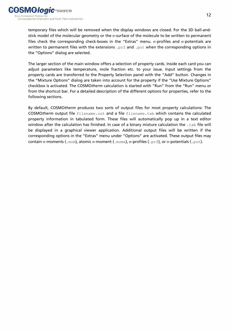
Example: Solid-liquid equilibrium curve of toluene and ethylbenzene Select toluene and ethylbenzene from the database or the File Manager. For both compounds, open the pure compound properties editor (select compound with a right mouse button click, then select “compound properties”) and enter data for the heat of fusion: For toluene, enter Tmelt = 178.16 K, ∆Hfus = 6.6107 (in SI units), and ∆Cpfus = 0.0486 (in SI units), for ethylbenzene, enter Tmelt = 178.20 K, ∆Hfus = 9.0709 (in SI units), and ∆Cpfus = 0.0515 (in SI units). In the SLE card, the compounds should be set automatically as first and second compound. Set the temperature to 140 K and transfer the settings to the “Property selection” with the Add button. Repeat the temperature setting and the transfer for temperatures 150 K, 160 K, 170 K, 178.16 K, and 178.20 K. The calculations for all temperatures will then be done in a single COSMOtherm run. The computed SLE points can be read from the .tab file:

130

140

150

160

170

180

190

0.0 0.1 0.2 0.3 0.4 0.5 0.6 0.7 0.8 0.9 1.0

x_Ethylbenzene

T [K

]Toluene

Ethylbenzene

Eutectic Point

For the graphic showing the eutectic point of toluene and ethylbenzene, the SLE points have been extracted from the table file and plotted in a single curve

30

FlatSurf: Surface Activity

With the FlatSurf option, the surface interaction energy of all compounds is computed at the interface of the two solvents or solvent mixtures. This is possible under the idealized assumption of a flat interface. The position of the solute at the interface is described by the distance z of the solute center from the interface, and orientation Γ of a fixed solute axis with respect to the surface normal direction. For such a given position of the compound a certain part of the molecular surface segments will be imbedded in phase S and the rest in phase S’. By sampling all relevant positions and orientations the minimum of the free energy of the solute at the flat interface of S and S’ can be found. The search for the optimal association of X at the interface can be extended to conformationally flexible molecules when the free energy differences between different solute conformers are taken into account. The minimum of the free energy of the solute at the flat interface of S and S’ and the total free energy of the solute at the flat interface of S and S’ can both be used as significant and thermodynamically rooted descriptors for the determination of surface activity in a solution. More details about the method can be found in the COSMOtherm Users Manul, section 5.10. COSMOtherm can use the experimental interfacial tension of the two solvent phases to improve the computed FlatSurf energies. This is possible with the IFT=value keyword. The value of the interfacial tension is expected to be in [dyne/cm]. Values for interfacial tensions of various solvent-solvent or air-solvent combinations can be found e.g. in the CRC Handbook of Chemistry and Physics7. Please note that the IFT option considerably increases the computational time of a FlatSurf calculation. To visualize the immersion and geometric partition of a solute in the two phases the option “Create Flatsurf VRML charge surface” can be checked. With this option, a VRML file will be written where the immersion depth z of the solute between the two solvent phases is represented graphically on the charge surface in the form of a black and white ring. The black part of the ring points towards FlatSurf solvent phase 1 and the smaller white part of the ring point towards FlatSurf solvent phase 2. Thus the ring indicates how the solute molecule is immersed in the two phases. The example on the right shows the immersion of a phenol molecule in a water (upper part) and a hexane phase (lower part).

31

Example: Calculate the Air-Water surface partition energy Select the the compounds water, benzene and chlorobenzene from the TZVP database. For air, select the vacuum.cosmo file. In the FlatSurf card, check “pure” for vacuum in phase 1 and for water in phase 2. Enter the value for the interfacial tension at the air-water interface (72.8 dyne/cm) into the appropriate field. To visualize the immersion of the solute between the two phases, check “Create Flatsurf VRML charge surface”. Add the settings to the Property selection window and run the program.

For each compound, the following descriptors are written to the output and table files:

• µXS,S’,res (Gmin): minimum of the free energy of the solute X at the flat interface of S and S’.

• GXS,S’ (Gtot): total free energy of the solute X at the flat interface of S and S’.

• aXV,S,S’ (Amin) contact area of the solute X with the flat interface of S and S’ at the free

energy minimum.

• aX (A): area of the COSMO-surface of solute X.

• z (Depth): distance of the center of solute X from the interface at the free energy minimum.

• k (K): number of orientations that were use to determine the surface interaction energy minimum of solute X.

If several conformers were used to compute a compound’s surface interaction energy, COSMOtherm will always write the name of the specific conformer to the table output, which was

able to achieve the lowest value of µXS,S’,res (Gmin). I.e. From the list of all conformers of a compound

the one with the lowest minimum free energy values at the flat interface of S and S’ will be listed. In contrast, GX

S,S’ (Gtot), the total free energy gain of the solute X at the flat interface is the thermodynamic average according to the interface partition sum of all conformers.

32

Density

The Density option uses the corrected molar liquid volume of the pure compounds to calculate

the pure compound liquid density ρ for all given compounds according to

iV~

Ai

ii

NV

MW~=ρ

where MWi is the molecular weight of the compound and NA is Avogadro’s constant. The corrected

molar liquid volume is computed from a Quantitative-Structure-Property-Relationship (QSPR)

which includes six generic QSPR parameters and one element specific parameter. iV

~

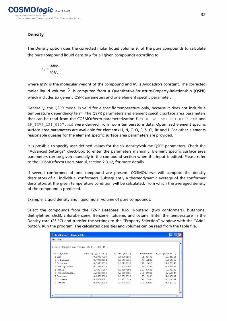
Generally, the QSPR model is valid for a specific temperature only, because it does not include a temperature dependency term. The QSPR parameters and element specific surface area parameters that can be read from the COSMOtherm parameterization files BP_SVP_AM1_C21_0107.ctd and BP_TZVP_C21_0107.ctd were derived from room temperature data. Optimized element specific surface area parameters are available for elements H, N, C, O, F, S, Cl, Br and I. For other elements reasonable guesses for the element specific surface area parameters are provided. It is possible to specify user-defined values for the six density/volume QSPR parameters. Check the “Advanced Settings” check-box to enter the parameters manually. Element specific surface area parameters can be given manually in the compound section when the input is edited. Please refer to the COSMOtherm Users Manul, section 2.3.12, for more details. If several conformers of one compound are present, COSMOtherm will compute the density descriptors of all individual conformers. Subsequently a thermodynamic average of the conformer descriptors at the given temperature condition will be calculated, from which the averaged density of the compound is predicted. Example: Liquid density and liquid molar volume of pure compounds. Select the compounds from the TZVP Database: h2o, 1-butanol (two conformers), butanone, diethylether, chcl3, chlorobenzene, Benzene, toluene, and octane. Enter the temperature in the Density card (25 °C) and transfer the settings to the “Property Selection” window with the “Add” button. Run the program. The calculated densities and volumes can be read from the table file.

33

Viscosity

The pure compound liquid viscosity is another property that can be calculated from QSPR. The descriptors for the liquid viscosity are the compound surface area as read from the COSMO file Ai, the second σ-moment of the compound Mi

2, the number of ring atoms in the compound NiRing and

the pure compounds entropy times temperature TSi, which is computed from the difference of the total enthalpy of mixture of the pure compound Hi and the chemical potential of the pure compound µi: TSi = -(Hi - µi). This QSPR model, like the Density QSPR model, does not include a temperature dependency term, so that the model is valid at a specific temperature only. Currently the parameterizations BP_SVP_AM1_C21_0107.ctd and BP_TZVP_C21_0107.ctd include the viscosity QSPR parameters for room temperature. User-defined values for the QSPR parameters can be specified manually when the “Advanced Settings” check-box is checked. For a compound with several conformers COSMOtherm will compute the viscosity descriptors of all individual conformers, followed by a thermodynamic averaging of the conformer descriptors at the given temperature condition to predict the averaged viscosity of the compound.

The σ-Moment Approach and QSPR Calculations

The σ-potentials of liquids can be represented by a Taylor-series with respect to σ,

∑=µ ml

Xl

lS

XS Mc

where the coefficients cS

l describe the specific corrections required for matrix S8. The σ-moments MiX

can be used to compute certain molecular properties via a Quantitative Structure Property Relationship (QSPR) approach9,10. COSMOtherm’s σ-moments can be correlated with properties such as lipophilicity, biological or environmental partition behavior like the octanol-water or soil-water partition, or the partition of a compound between the blood-brain barrier. The QSPR coefficients cS

l for a certain property can be determined from a multi-linear regression of the σ-moments with a sufficient number of experimental data. For a compound X a property log(P) is calculated via:

(13)

16415314213112

4113102918

67564534231201)log(

cMcMcMcMc

McMcMcMc

McMcMcMcMcMcMcP

XHBdon

XHBdon

XHBdon

XHBdon

XHBAcc

XHBacc

XHBacc

XHBacc

XXXXXXX

+++++

++++

++++++=

where Mi

X is the ith σ-moment of compound X and MHBacc iX and MHBdon i

X are the ith hydrogen bonding acceptor and donor moments of compound X. Thus, a maximum of 16 coefficients is available to do the σ-moments QSPR calculation. However, a multilinear regression can usually be done with only 5 descriptors (M0 (area), M2 (sig2), M3 (sig3), MHBacc3, MHBdon3) to avoid over-parameterization. For a detailed description of σ-moments and property calculation via σ-moment QSPR refer to sections 5.4 and 5.5 of the COSMOtherm User’s Manual) The current COSMOtherm release includes QSPR coefficient files for the following properties, parameterized on the Turbomole BP-SVP-AM1 COSMO level:

34

• logPOW.prop: Octanol-water partition coefficients logPOW.

• logBB.prop: Blood-Brain partition coefficients logPBB.

• logKOC.prop: Soil-Water partition coefficients logKOC.

• logKIA.prop: Intestinal absorption coefficients logKIA.

• logKHSA.prop: Plasma-protein (human serum albumin) partition coefficients logKHSA. Furthermore, the COSMOtherm release includes a number of QSPR property files holding QSPR coefficients for the five Abraham parameters and the definition of thermodynamic partition properties via the six Abraham coefficients, for both computational COSMO levels BP-TZVP and BP-SVP-AM1. For an automatic QSPR calculation of the selected compounds COSMOtherm offers two options. Global QSPR option: This option is activated when the required property in the “QSPR” menu is checked. By default, the computed property value will be listed in the compound section of the COSMOtherm output file. Additionally, a tabulated output file with the extension .mom will be

written, listing the molecular σ-moments and, in the last column, the computed property. Currently, there can always one QSPR property only be calculated in a single run.

Mix-QSPR option: This option can be selected from the Mix-QSPR property card. It is closely related to the global QSPR option, but the Mix-QSPR option writes the results to the mixture section of the COSMOtherm output file as well as to the COSMOtherm table file, but not to the molecules σ-moment files (.mom). If mixture composition and temperature are not specified (which is the default), COSMOtherm calculates the QSPR property chosen from the menu for all molecules, i.e. for all conformers of the compounds individually, giving the same results as the global QSPR option. However, with the Mix-QSPR option, temperature and mixture composition can be specified when the “Advanced Settings” check-box is checked. If this is done, the QSPR property will be calculated for all compounds by averaging the property according to the Boltzmann distribution of the conformers at the given temperature and mixture concentration. This will result in different values for the QSPR property only for compounds for which more than one conformer is present.

35

Similarity

With this option, COSMOtherm will calculate a molecular similarity of two compounds based on σ-

profiles or σ-potentials. The σ-profile similarity factor Si,j is calculated as the normalized overlap integral of the σ-profiles pi(σ) and pj(σ) of the two compounds i and j:

ji

ji

ji AA

dpp

S∫

+∞

∞−

σσσ

=

)()(

, (14)

Si,j will be small if the overlap between the compounds σ-profiles is small. In addition, the similarity factor given by eq. (14) is corrected by a factor SH

i,j taking into account the difference in the apparent hydrogen bonding donor and acceptor capacities of the two compounds and by a factor SA

i,j taking into account size differences between the two compounds i and j. The similarity factor Si,j is printed to the mixture output section of the COSMOtherm output file below the compound output block of the first compound given in the similarity command. If several conformers are present for a compound, the similarity factor will be computed for all possible combinations of the conformers and the overall compound similarity factor is averaged from the computed conformer similarity factors. Furthermore, COSMOtherm can also calculate a σ-potential based similarity factor for two compounds. The COSMOtherm σ-potential similarity factor SP

i,j is defined as the sum of the differences between the two pure compound σ-potentials µi(σ) and µj(σ):

( ) ( ) ⎟⎟⎠

⎞⎜⎜⎝

⎛σµ−σµ−= ∑

+=

−=

02.0

02.0, exp

m

mmjmi

PjiS (15)

SP

i,j will be small if the overlap between the compounds σ-potentials is small. The similarity factor SP

i,j is printed to the mixture output section of the COSMOtherm output file below the compound output block of the first compound given in the similarity command and, additionally, to the COSMOtherm table file. As an alternative to the molecular non-specific cut-off function of eq. (15) the σ-potential based similarity factor can also be calculated as a solute-specific σ-potential similarity. SP

i,j(pk) is the σ-potential similarity for compounds i and j weighted by the σ-profile pk.

36

Using your own COSMO files There are several ways to make your own COSMO files available in COSMOthermX. You can

• select COSMO or compressed COSMO files from any directory on your system using the File Manager,

• add your own database(s), • extend existing databases.

For all options there are a few prerequisites you have to take into account to ensure that the COSMOtherm calculations run correctly:

• Ensure that all COSMO files you want to use come from the same quantum chemical level. Combine only COSMO files from BP-TZVP cosmo or gas phase calculations with COSMO files from the BP-TZVP-COSMO database. Combine COSMO files from the BP-SVP-AM1 database only with your own COSMO files from BP-SVP-AM1 cosmo or gas phase calculations. Note that .cosmo and .ccf files can be mixed in the databases.

• Gas phase energies, which should be used if properties involving a gas phase (VP, VLE, Henry law constant, gas solubility) are calculated and experimental vapor pressure data are not available, should be saved into an .energy file. The gas phase energies must be from the quantum chemical level that has been used for the COSMO calculations, e.g. BP-TZVP for gas phase calculations and BP-TZVP-COSMO for COSMO calculations. The default unit for gas phase energies is [Hartree].

• Experimental vapor pressure data or other experimental data can be saved into a .vap file. Create the .vap file manually using any text editor, or use the “Compound Properties” menu from the right mouse button context menu for a selected compound to enter property data for a compound.

• Vapor Pressure / Property and energy files should be located in the same directory as the .cosmo files.

Using the File Manager

COSMO or compressed COSMO files from Quantum Chemical calculations can be selected from any directory on your system using the File Manager in the compound section of COSMOthermX.

Adding your own Databases

You can add your own database(s) to COSMOthermX in the “Settings” dialog. In the “Databases” pane, select “Add”. You will be presented with a new dialog where you have to enter a name for the database, point to the location of the database directory and the database index file, and specify a parameterization to be used with this database.

37

Databases with BP-SVP-AM1 parameterization will then be available with the “SVP Database” button in the compound section, and databases with BP-TZVP-COSMO parameterization will be available with the “TZVP Database” button. Before you add your database to COSMOthermX you have to make some preparations:

• Collect all .cosmo / .ccf files that belong to the database in a single directory. If you have .energy or .vap files for the compounds, also put them in this directory. Ensure that all .cosmo / .ccf files are calculated on the same quantum chemical level, and that the .energy files come from corresponding gas phase calculations.

• For conformers of a compound to be identified as conformers, the .cosmo or .ccf files have to be named with the compound name followed by a number, e.g. ethanol0.ccf, ethanol1.ccf and so on. Then the conformers will be treated as a single compound if the “Activate Conformers Treatment” box is checked in the compound section.

• Prepare the database index file. This is a plain ASCII text file in the “comma separated file“ (CSV) format, i.e. all entries are separated by commas “;”. The database index file has the format:

COSMO-Name ; CAS-Number ; MW ; Formula ; Alternative_Name ; Conformer1_Name ; Conformer1_Alternative_Name; Conf2_Name ; Conf2_AltName ; Conf3_Name ; Conf3_AltName ; Conf4_Name ; Conf4_AltName ; …

I.e. the additional conformers are attached to the database index list shown above as additional entries, with two additional fields for each conformer: first the conformers COSMO-filename (without extension) and then, separated by a comma “;”, the conformers trivial name. Up to nine additional conformers can be processed. For example, the compound valine that consists of two conformers is given in the database index file as

VALINE0;000072-18-4;117.1474;C5H11NO2;L-VALINE-conformer-0;VALINE1;L-VALINE-conformer-1;;;;;;;;;;;;;

• The database directory and the database index file must have identical names and must be

located in the same main directory, i.e. the database directory <MY-DATABASE> has to be a subdirectory of the directory where the database index file <MY-DATABASE.csv> is located.

Extend the existing Databases

The databases, your own as well as those that come with the COSMOtherm release, can be extended with .ccf or .cosmo files. Just copy the .cosmo (and, if available, .energy and .vap files) into the database directory. Take care to add only files to existing databases which match the quantum chemical level of the database. To make the added compounds available in COSMOthermX, you also have to manipulate the database index file, e.g. BP-TZVP-COSMO.csv.

38

Atom weighting Due to the additive nature of σ-profiles it is possible to approximately describe molecules which are not contained in your database or which are simply to large to be calculated by adjusting the ‘importance’ of other molecules’ atoms or even blending together multiple secondary molecules. The result of this process is either stored in a so-called weight string (for a single molecule) or in a COSMO meta-file with the extension .mcos (for a molecule blended together from multiple molecules). For more information about atom weighting please refer to the COSMOtherm manual. As the manual generation of weight strings usually involves quite a lot of counting and double checking, COSMOthermX includes COSMOweight, an interactive graphical tool, which can greatly improve your working speed when dealing with medium-sized molecules. Using COSMOweight to edit weight strings: Right-click a compound in your compound list and select “Edit weight string”. You will be presented with a new window showing a ball-and-stick-model of the selected compound. Disabled atoms will be displayed with dotted lines and their bonds black, whereas atoms with higher importance than 1 will pulse. For a brief despription of navigation in 3D-space have a look at the section “Using COSMOview”.

• Atom weights can be increased by left-clicking and decreased by right-clicking single atoms. Alternatively, you can point your mouse at an atom and type the number you would like to assign to its weight on your keyboard, you can directly edit the textfield. In some cases, you may want to have only a small part of the molecule activated.

• Instead of manually assigning each unwanted atom a weight of 0, just click the “Set 0”

button . • Reseting all weights to their initial value of 1 is possible by pressing the “Set to 1” button

. Please note that COSMOweight will sometimes display warning messages related to the structure of the molecule being edited. These are only supposed to help spotting chemical and/or logical mistakes - as you will know, the structure itself is not used in any COSMOtherm calculation. Using COSMOweight as a meta file editor: This mode can either be accessed by right-clicking an .mcos file in your compound list and selecting “Edit .mcos file”, by selecting one or more .cosmo or .ccf files from your compound list, right-click and select “Edit .mcos file” or via “Tools-mcos file editor”. In the latter case, open an existing .mcos file by

clicking “Open” ( ) or start from

scratch by adding a first molecule ( ). Additionally to editing single weight strings (cf. “Using COSMOweight to edit weight strings”) you can add further

molecules or remove ( ) as well as switch between them in the “Molecule” pull-down menu. When you are done,

click Save ( ) to generate a .mcos file.

39

Saving .mcos files: In the “Save” dialog, there are three different options to save the .mcos file. These options control where COSMOtherm will look for the .cosmo and .ccf files (henceforth “source files”) you used.

• absolute: You can always save your work with absolute paths. The absolute paths of the source files are written to the file, which means, that your sources can be spread over different volumes and you are able to move your .mcos file wherever you please. However, if the source files themselves are moved, or - more importantly - you try to use the .mcos file on another computer with a different folder hierarchy, you will run into problems.

• relative to file: This is the default if you do not use a fragment directory. Source files will have to be located in the folder you save the .mcos file to or in subfolders. You can move this kind of .mcos file to different directories, even different computers, if you also copy the source files.

• relative to fragment directory: This option gives you ultimate portability while still avoiding the need to copy data. All source files used have to be located in the folder set as “fragment directory” in the “Settings” dialog. You can move the .mcos file everywhere, as long as you keep with your “fragment directory” settings. If you use a lot of meta-files, this is the way to go. If you did not set a fragment directory, this option will be disabled. Please note that, you may want to set your fragment directory to the COSMO-DATABASE folder or one of its subfolders. The .mcos-files shipped with COSMOthermX will not work unless you either disable the use of a fragment directory or set the database with parameterization as a fragment directory, e.g. '<COSMOTHERM_HOME>/DATABASE-COSMO/BP-SVP-AM1>'.

Problems when using .mcos files: If COSMOtherm or COSMOweight complain about missing files when using previously saved .mcos files, you are likely trying to open a kind of .mcos file which is saved

• “relative to fragment directory” (cf. Saving .mcos files) while you either disabled the use of a fragment directory in COSMOthermX or set a wrong path;

• “relative to file” while you have set a fragment directory in COSMOthermX • “absolute”, but created on a different computer or before making changes to the folder

hierarchy.

1 “COSMO: A New Approach to Dielectric Screening in Solvents with Explicit Expression for the Screening Energy and its Gradients.” A. Klamt, G. Schüürmann, J. Chem. Soc., Perkin Trans. 2 1993, 799. 2 “Refinement and Parameterization of COSMO-RS.” A. Klamt, V. Jonas, T. Bürger, J. W. C. Lohrenz, J. Phys. Chem. A. 1998, 102, 5074. 3 “Fast Solvent Screening via Quantum Chemistry: COSMO-RS Approach.“ F. Eckert, A. Klamt, AIChE J. 2002, 48, 369. 4 “COSMO-RS: a novel and efficient method for the a priori prediction of thermophysical data of liquids.“, A. Klamt, F. Eckert, Fluid Phase Equilib. 2000, 172, 43. 5 “COSMO implementation in TURBOMOLE: Extension of an efficient quantum chemical code towards liquid systems”, A. Schäfer, A. Klamt, D. Sattel, J. C. W. Lohrenz, F. Eckert, Phys. Chem. Chem. Phys. 2000, 2, 2187. 6 J. J. P. Stewart, MOPAC2002 program package, Fujitsu Corp. 2002. (fqspl.com.pl/linmopac/overview.html) 7 Lide, R. D. (Ed.), CRC Handbook of Chemistry and Physics, CRC Press, 2000. 8 “Conductor-like Screening Model for Real Solvents: A New Approach to the Quantitative Calculation of Solvation Phenomena”, A. Klamt, J. Phys. Chem., 1995, 99, 2224.

40

9 “Cosmo-RS: A novel view to physiological solvation and partition questions“, A. Klamt, F. Eckert, M. Hornig, J. Computer Aided Mol. Design 2001, 15, 355. 10 “COSMO-RS: A Novel Way from Quantum Chemistry to Free Energy, Soluility, and General QSAR-Descriptors for Partitioning“, A. Klamt, F. Eckert, in Rational Approaches to Drug Design, H.-D. Höltje and W. Sippl, Ed., Prous Science, Barcelona, 2001, 195.