Cosmological Evolutionof the

Fine Structure Constant

Chris Churchill(Penn State)

= e2/hc = (z-0)/0

In collaboration with: J. Webb, M. Murphy, V.V. Flambaum, V.A. Dzuba,J.D. Barrow, J.X. Prochaska, & A.M. Wolfe

Your “Walk Away” Info

1. 49 absorption cloud systems over redshifts 0.5–3.5 toward 28 QSOs compared to lab wavelengths for many transitions

2. 2 different data sets; low-z (Mg II, Mg I, Fe II) high-z (Si II, Cr II, Zn II, Ni II, Al II, Al III)

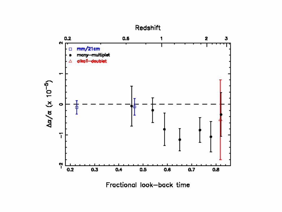
3. Find = (–0.72±0.18) × 10-5 (4.1) (statistical)

4. Most important systematic errors are atmospheric dispersion (differential stretching of spectra) and isotopic abundance evolution (Mg & Si; slight shifting in transition wavelengths)

5. Correction for systematic errors yields stronger evolution

Executive Summary

1. History/Motivations2. Terrestrial and CMB/BBN Constraints3. QSO Absorption Line Method4. Doublet Method (DM) & Results5. Many-Multiplet Method (MM) & Results6. Statistical and Systematic Concerns7. Concluding Remarks

Very Brief HistoryMilne (1935, 1937) and Dirac (1937) postulate that the gravitation constant, G, varied with time.

Dirac’s “Large Number Hypothesis” led to theoretical work, development of scalar-tensor generalizations of Einstein’s general relativity (Brans & Dicke 1961)

Jordon (1937, 1939) considers other coupling constants

Landau (1955) proposes variations in connected to renormalization in quantum electrodynamics (QED)

Modern theories unify gravity with other forces…

Multi-dimensional Unification

Quantization of gravitational interactions…

Early attempts invoke (4+D)-dimensional curved space-times similar to Kaluza-Klein scenario for E&M + gravity, weak, strong, vary as inverse square of dimension scale

Evolution of scale size of extra dimensions drives variability of these coupling constants in the 4-dimensional subspace of Kaluza-Klein and superstring theories

Cosmological variation of may proceed at different rates at different points in space-time (Barrow 1987; Li & Gott 1998)

Multi-dimensional Unification

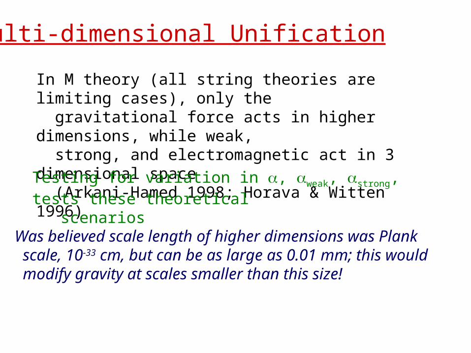
In M theory (all string theories are limiting cases), only the gravitational force acts in higher dimensions, while weak, strong, and electromagnetic act in 3 dimensional space (Arkani-Hamed 1998; Horava & Witten 1996)

Testing for variation in , weak, strong, tests these theoretical scenarios

Was believed scale length of higher dimensions was Plank scale, 10-33 cm, but can be as large as 0.01 mm; this would modify gravity at scales smaller than this size!

Scalar Theories

Bekenstein (1982) introduced a scalar field that produces a space-time variation in electron charge (permittivity of free space). Reduces to Maxwell’s theory for constant .

Variation in coupled to matter density and is therefore well suited for astronomical testing (Livio & Stiavelli 1998).

Also can be applied to other coupling constants.

All require assumptions- there is no single self-consistent scalar field theory incorporating varying ; theoretical limits must all be quoted in conjuction with theoretical framework

Self-consistency relations for M theory require /2 ~ G/G

Varying Speed of Light Theories

Motivation is to solve the “flatness” and “horizon” problems of cosmology generated by inflation theory (Barrow 1999).

Two benefits: (1) prevents from dominating during the radiation epoch(2) links cosmological acceleration (Perlmutter et al 1998) to a

varying

Theory allows variation in to be ~10-5 H0 at redshift z=1, and for to dominate today and produce acceleration. The factor of 10-5 comes from the ratio of radiation to matter density today.

c2, where is the cosmological constant, acts as a “stress”. Changes in c convert the energy density into radiation (Barrow & Magueijo 2000)

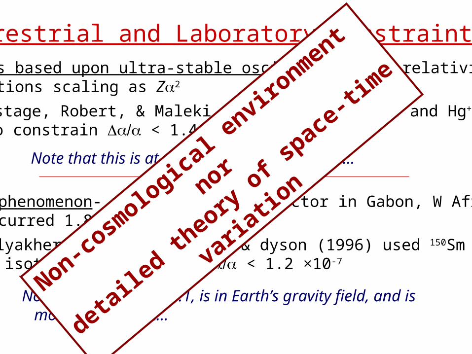
Terrestrial and Laboratory ConstraintsClock rates based upon ultra-stable oscillators with relativistic corrections scaling as Z2

Prestage, Robert, & Maleki (1995) used H-maser and Hg+

to constrain < 1.4 ×10-14

Oklo phenomenon- natural fission reactor in Gabon, W Africa, occurred 1.8 Bya

Note that this is at z=0 in Earth’s gravity field…

Shlyakher (1976) and Damour & dyson (1996) used 150Sm isotope to constrain < 1.2 ×10-7

Note that this is at z~0.1, is in Earth’s gravity field, and is model dependent…

Non-cosm

ological e

nvironmen

t

nor

detaile

d theo

ry of s

pace-ti

me varia

tion

Early Universe (CMB and BBN)

• The ionization history of the universe, either postponing (smaller) or delaying (larger) the redshift of recombination (z~1000). This would alter the ratio of baryons to photons and the amplitude and position of features in the CMB spectrum (Kujat & Scherrer 2000)

However, electromagnetic contribution to p-n mass difference is very uncertain

A different value of would change:

• The electromagnetic coupling at time of nucleosynthesis (z~108-109). Assuming scales with p-n mass difference, 4He abundance yields / < 9.9 ×10-5 (Kolb et al 1986)

(implications)

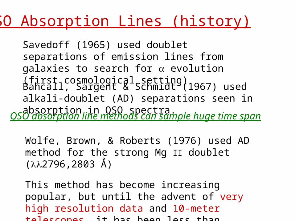
QSO Absorption Lines (history)

Savedoff (1965) used doublet separations of emission lines from galaxies to search for evolution (first cosmological setting)

Bahcall, Sargent & Schmidt (1967) used alkali-doublet (AD) separations seen in absorption in QSO spectra.

QSO absorption line methods can sample huge time span

Wolfe, Brown, & Roberts (1976) used AD method for the strong Mg II doublet (2796,2803 Å)

This method has become increasing popular, but until the advent of very high resolution data and 10-meter telescopes, it has been less than conclusive, = (2±7) ×10-5

So… what are QSO absorption lines?

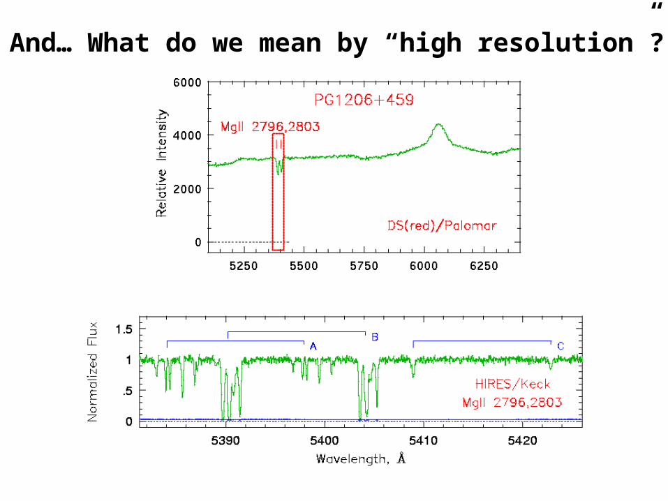
And… What do we mean by “high resolution”?

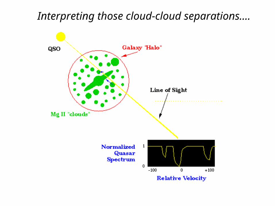
Interpreting those cloud-cloud separations….

And, of course…

Keck Twins10-meter Mirrors

The Weapon.

The High Resolution Echelle Spectrograph (HIRES)

2-Dimensional Echelle Image

Dark features are absorption lines

The “Doublet Method” ex. Mg II 2796, 2803

A change in will lead to a change in the doublet separation according to

where ()z and ()0 are the relative separations at redshift z and in the lab, respectively.

Si IV 1393, 1402

Example spectrum of this Mg II system (z=1.32)

We model the complex profiles as multiple clouds, usingVoigt profile fitting (Lorentzian + Gaussian convolved) to obtain component redshifts (velocities).

Lorentzian is natural line broadening Gaussian is thermal line broadening (line of sight)

Example of a Si IV system at z=2.53 used in the analysis of Murphy et al (2001)

Si IV Doublet Results: = –0.51.3 ×10-5

(Murphy et al 2001)

The “Many Multiplet Method”

A change in will lead to a change in the electron energy, , according to

where Z is the nuclear charge, |E| is the ionization potential, j and l are the total and orbital angular momentum, and C(l,j) is the contribution to the relativistic correction from the many body effect in many electron elements.

Note proportion to Z2 (heavy elements have larger change)

Note change in sign as j increases and C(l,j) dominates

Ez = Ec + Q1Z2[R2-1] + K1(LS)Z2R2 + K2(LS)2Z4R4

Ec = energy of configuration center

Q1, K1, K2 = relativistic coefficients

L = electron total orbital angular momentum

S = electron total spin

Z = nuclear charge

R = z/

The energy equation for a transition from the ground state at a redshift z, is written

A convenient form is: z = 0 + q1x + q2y

z = redshifted wave number

x = (z/0)2 - 1 y = (z/0)4 - 1

0 = rest-frame wave number

q1, q2 = relativistic correction coefficients for Z and e- configuration

Mg II 2796Mg II 2803Fe II 2600Fe II 2586Fe II 2382Fe II 2374Fe II 2344

Typical accuracy is 0.002 cm-1, a systematic shift in these values would introduce only a ~ 10-6

A precision of ~ 10-5 requires uncertainties in 0 no greater than 0.03 cm-1 (~0.3 km s-1)

Well suited to data quality… we can centroid lines to 0.6 km s-1, with precision going as 0.6/N½ km s-1

Anchors & Data Precision Shifts for ~ 10-5

Advantages/Strengths of the MM Method

1. Inclusion of all relativistic corrections, including ground states, provides an order of magnitude sensitivity gain over AD method

2. In principle, all transitions appearing in QSO absorption systems are fair game, providing a statistical gain for higher precision constraints on compared to AD method

3. Inclusion of transitions with wide range of line strengths provides greater constraints on velocity structure (cloud redshifts)

4. (very important) Allows comparison of transitions with positive and negative q1 coefficients, which allows check on and minimization of systematic effects

= (–0.72±0.18) × 10-5 (4.1) (statistical)

Possible Systematic Errors

1. Laboratory wavelength errors2. Heliocentric velocity variation3. Differential isotopic saturation4. Isotopic abundance variation (Mg and Si)5. Hyperfine structure effects (Al II and Al III)6. Magnetic fields7. Kinematic Effects8. Wavelength mis-calibration9. Air-vacuum wavelength conversion (high-z sample)10. Temperature changes during observations11. Line blending12. Atmospheric dispersion effects13. Instrumental profile variations

Isotopic Abundance Variations

There are no observations of high redshift isotopic abundances, so there is no a priori information

Focus on the “anchors”

We re-computed for entire range of isotopic abundances from zero to terrestrial. This provides a secure upper limit on the effect.

Observations of Mg (Gay & Lambert 2000) and theoretical estimates of Si in stars (Timmes & Clayton 1996) show a metallicity dependence

Corrected Uncorrected

This is because all Fe II are to blue of Mg II anchor and have same q1 sign (positive)

Leads to positive

For high-z data, Zn II and Cr II areTo blue and red of Si II and Ni II anchors and have opposite q1 signs

Correction for Isotopic Abundances Effect low-z Data

a = pixel size [Å] , = slit width arcsec/pix,ψ = angular separation of and 2 on slit,θ = angle of slit relative to zenith

Atmospheric Dispersion

Blue feature will have a truncated blue wing!

Red feature will have a truncated red wing!

This is similar to instrumental profile distortion, effectively a stretching of the spectrum

Causes an effective stretching of the spectrum which mimics a non-zero

Correction for Atmospheric Distortions Effect low-z Data

Corrected Uncorrected

This is because all Fe II are to blue of Mg II anchor and have same q1 sign (positive)

Leads to positive

For high-z data, Zn II and Cr II areTo blue and red of Si II and Ni II anchors and have opposite q1 signs

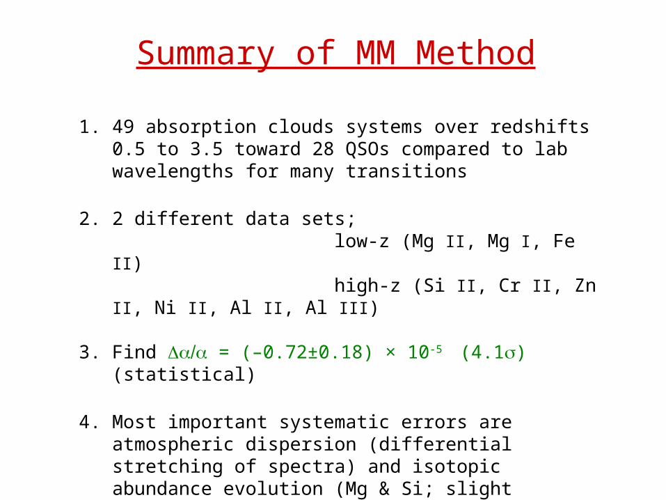
Summary of MM Method

1. 49 absorption clouds systems over redshifts 0.5 to 3.5 toward 28 QSOs compared to lab wavelengths for many transitions

2. 2 different data sets; low-z (Mg II, Mg I, Fe II) high-z (Si II, Cr II, Zn II, Ni II, Al II, Al III)

3. Find = (–0.72±0.18) × 10-5 (4.1) (statistical)

4. Most important systematic errors are atmospheric dispersion (differential stretching of spectra) and isotopic abundance evolution (Mg & Si; slight shifting in transition wavelengths)

5. Correction for systematic errors yields stronger evolution