CoSiNE Manual

Zhegui Wang, Fei Chai

Oct 2017

Table of Contents 1 Overview .................................................................................................................................................... 2

2 New Version of the Code ........................................................................................................................... 2

2.1 code cleaning ...................................................................................................................................... 3

2.1 code structure ...................................................................................................................................... 3

2.1.1 cosine.F90 .................................................................................................................................... 3

2.1.2 cosine_init.F90 ............................................................................................................................. 3

2.1.3 cosine_mod.F90 ........................................................................................................................... 4

3 Model Setup ............................................................................................................................................... 4

3.1 compiling the code .............................................................................................................................. 4

3.2 parameter file: cosine.in ...................................................................................................................... 4

3.2.1 global switches ............................................................................................................................. 4

3.2.2 phytoplankton .............................................................................................................................. 5

3.2.3 zooplankton .................................................................................................................................. 6

3.2.4 other ............................................................................................................................................. 7

3.3 Initial Condition .................................................................................................................................. 7

3.3.1 ihot=0 ........................................................................................................................................... 7

3.3.2 ihot=1 or ihot=2 ........................................................................................................................... 8

3.4 Boundary Condition ............................................................................................................................ 8

3.5 Loading ............................................................................................................................................... 9

4 Model Kinetics ......................................................................................................................................... 10

2.1 Phytoplankton: S1 and S2 ............................................................................................................. 10

2.2 Zooplankton: Z1 and Z2 ............................................................................................................... 13

2.3 Dissolved Nutrients: NO3, NH4, SiO4 and PO4 .......................................................................... 14

2.4 Detritus Organic Matter: DN and DSI .......................................................................................... 15

2.5 Oxygen and Carbon System: DOX, CO2, and ALK .................................................................... 15

2.6 Temperature Adjustment ............................................................................................................... 16

References ................................................................................................................................................... 16

1 Overview

CoSiNE stands for Carbon, Silicate, Nitrogen Ecosystem, which was originally developed by Prof. Fei Chai

(U. of Maine) for modeling the ocean biogeochemical processes for the equatorial Pacific and the Pacific

Ocean (Chai, Dugdale et al. 2002, Chai, Jiang et al. 2003, Chai, Jiang et al. 2007). In CoSiNE model, there

are 13 state variables including 2 phytoplankton species (S1 and S2), 2 zooplankton species (Z1 and Z2), 3

nitrogen forms (NO3, NH4 and DN (detritus nitrogen)), 2 silicon forms (SiO4 and DSi (detritus silicon))

and 1 phosphorus form (PO4), dissolved Oxygen (DOX), total carbon dioxide (CO2) and total alkalinity

(ALK). The symbol and numbering in CoSiNE model for each variable are listed in Table 1. For

understanding the underlying biological processes, users are strongly encouraged to read through the model

kinetics detailed in Section 4. This will be very helpful in the process of tuning the model for achieving a

specific goal.

To successfully run CoSiNE model, one needs to prepare inputs for both hydrodynamic model (SCHISM)

and biochemical model (CoSiNE). Normally, we setup the hydrodynamic model for the physical part first.

After reasonable calibration, we then add CoSiNE model for the biological part. You can refer to SCHISM

website schism.wiki on how to build up and run the SCHISM model. In this document, we focus on how

to build up CoSiNE model.

Table 1. List of CoSiNE model variables

Name of State

Variables

Symbol Tracer Numbering in

SCHISM (within

CoSiNE module)

Unit

Nitrate NO3 1 mmol/m3

Silicate SiO4 2 mmol/m3

Ammonium NH4 3 mmol/m3

Small Phytoplankton S1 4 mmol/m3

Diatom S2 5 mmol/m3

Microzooplankton Z1 6 mmol/m3

Mesozooplankton Z2 7 mmol/m3

Detritus Nitrogen DN 8 mmol/m3

Detritus Silicon DSi 9 mmol/m3

Phosphate PO4 10 mmol/m3

Dissolved Oxygen DOX 11 mmol m-3

Dioxide Carbon CO2 12 mmol m-3

Alkalinity ALK 13 meq/m3

2 New Version of the Code

The CoSiNpE model was rewritten by Zhengui Wang on 04/13/2017 based on a version from Qianqian Liu

with code name “cosine.F90.R1”. The revised model was tested continuously in San Francisco Bay and

compared with Qianqian’s original results to make sure that there are no bugs introduced.

2.1 code cleaning

The original code was cleaned in the following aspects:

1) Separating model parameters from the code

This will make model easy to use and there is no need to recompile the code when changing

parameter values.

2) Reorganizing the model

The new structure of code is consistent with SCHISM style. Also, it makes future maintenance

and development of the model easier

3) Reformatting the code

It makes the code consistent and easy to read

4) Removing redundant/unnecessary variables and renaming all variables of bad practice

5) Adjusting/Rewriting some parts of the model

Inside the original code, better coding is applied to make the code concise and easy to read. This

is important to avoid making mistakes in future new coding.

6) Fixing bugs.

In this new version code, variable names are consistent inside the code and manual. Normally, we will use

capital letters for CoSiNE variables and most kinetic terms (eg. mortality and grazing terms). All model

parameters, model switches and functional terms are in lower case. In the code, all the kinetic terms are

stored in temporary variables, but one may be interested in investigating these terms in certain applications.

In this case, one can output the value of these variables and we will try to add this functionality in future

model development.

2.1 code structure

The original CoSiNE code was split into 3 files: cosine.F90, cosine_mod.F90 and cosine_init.F90. In

addition, the model parameters are separated from the model as a model input file.

2.1.1 cosine.F90

Subroutines in cosine.F90:

cosine: main routine for CoSiNE model

o2flux: calculate O2 flux

co2flux: calculate CO2 flux

ph_zbrent: calculate ph value (aquatic chemistry)

ph_f: nonlinear equations for ph

ceqstate: calculate seawater density

Inside this file, there are 6 subroutines. The main subroutine is cosine, which was invoked in SCHISM.

Inside subroutine cosine, it conducts all computations for biological processes and passes the results back

to SCHISM for physical transport. The subroutines o2flux and co2flux are used to calculate O2 and CO2

air-sea exchange fluxes. These two subroutines are called by subroutine cosine. The other three subroutines

(ph_zbrent, ph_f and ceqstate) are invoked by subroutine co2flux to calculate CO2 flux.

2.1.2 cosine_init.F90

Subroutines in cosine_init.F90:

cosine_init: variables allocation and initialization

read_cosine_param: read CoSiNE parameters from parameter input file cosine.in

read_cosine_stainfo: read information for CoSiNE output stations

check_cosine_parame: dump CoSiNE parameters for checking

pt_in_poly: determine if a point is in a polygon

In subroutine cosine_init, model variables of arrays are allocated and initialized to zero. The subroutine

read_cosine_param reads in model specification numbers and model parameters from input file cosine.in,

while check_cosine_param outputs all model parameters for double checking and reference. The subroutine

read_cosine_stainfo reads in station information for CoSiNE specific outputs. Some pre-processing is done

in this subroutine and subroutine pt_in_poly is called.

2.1.3 cosine_mod.F90

There is only one module cosine_mod inside this file. This module is to declare all model parameters and

global variables. However, the state variables of CoSiNE model are also declared in this module for

convenience, even though they are not global variables.

3 Model Setup

3.1 compiling the code

In order to run the model, we need to turn on the CoSiNE submodule inside the SCHISM. First, we

uncomment the following two lines for CoSiNE model in file trunk/mk/include_modules. Second, we go

to directory trunk/src and type command make to compile. This will generate an executable for CoSiNE.

# CoSINE

USE_COSINE = yes

EXEC := $(EXEC)_COS

3.2 parameter file: cosine.in

CoSiNE model needs a parameter input file cosine.in. The format of cosine.in is written to be consistent

with SCHISM parameter input file param.in. A sample file, cosine.in.sample, is provided with the source

code. These parameters include some functional switches and kinetic coefficients for biological processes.

The parameter values in cosine.in.sample are based on Qianqian’s San Francisco Bay application

“2011_R1”. Inside cosine.in, a simple description is given for each parameter and more detailed information

will be added in the future model development. In addition, more switches for new functions may be added

in this file.

3.2.1 global switches

niter (int)

Number of sub-cycles for CoSiNE kinetics processes. It divides the SCHISM time step dt into niter cycles

and each cycle has a time step dt/niter. Usually, one will use niter=1. It gives CoSiNE model the time step

of SCHISM hydrodynamics, which is sufficient to resolve biogeochemical processes in most cases.

idelay (int)

When idelay=1, the mesozooplankton grazing response to S2, DN and DSi is delayed by 7 days. The reason

is that zooplankton consumption of phytoplankton during its early life stages is much smaller than during

its adult stages. In the model, the concentrations of S2, DN, DSi and Z2 seven days earlier are used to

calculate the grazing rate of Z2.

ibgraze (int)

When ibgraze=1, the mortality rates of S2 and Z2 are increased by 2 times in the bottom part of water

column. This is to mimic bottom grazing such as clams.

idapt (int), alpha_corr (double) and zeptic (double)

When idapt=1, phytoplankton light adaptation is used to increase growth rate when light intensity is weak.

Alpha_corr and zeptic are two parameters for light adaptation. If idapt=0, these two parameters are not used.

iz2graze (int)

When iz2graze=0, mesozooplankton grazing on S2, DN and DSi is set to be zero.

iout_cosine (int) and nspool_cosine (int)

When iout_cosine=1, model will output time series for intermediate variables and CoSiNE variables at

specified locations. An input file cstation.in that has a similar format of SCHISM station.bp is needed.

nspool_cosine (number of time steps) is the interval for the output. The CoSiNE output is done on each

process under parallel computing. It needs a post-processing to combine all the output into one file

cstation.out. A combining script combine_cosine_output.f90 is provided along with the code to perform

this task.

ico2s (int)

When ico2s=1, CO2 is also taken into consideration for phytoplankton growth. If CO2 concentration is too

low, it can limit phytoplankton growth. Normally, you can turn this function off by using ico2s=0 if CO2

is not a limiting factor in your application.

ispm (int), spm0 (double)

CoSiNE model needs the concentration of suspended particulate matter (SPM) to calculate the light

extinction coefficient for phytoplankton. This parameter is to provide the method on how SPM is given.

When ispm=0, model will use constant SPM concentration specified by spm0. When ispm=1, a spatially

varying SPM will be used and user needs to provide an additional input file SPM.gr3 which has a similar

format to SCHISM grid. When ispm=2, the model will used SPM concentration from sediment model. In

this case, the SCHISM module SED needs to be turned on. The user should provide all the input file for

sediment model and calibrate it.

icheck (int)

When icheck=1, model will output all parameter values used in the code. This flag is to check whether the

model parameters read into the model are correct.

3.2.2 phytoplankton

gmaxs1 (double) and gmaxs2 (double)

Maximum growth rate for S1 and S2

pis1 (double) and pis2 (double)

Ammonium inhibition factor for S1 and S2

kno3s1, knh4s1, kpo4s1, kco2s1 and kno3s2, knh4s2, kpo4s2, kco2s2, ksio4s2 (double)

These parameters are the half saturation constants of nutrients for phytoplankton.

kns1 (double) and kns2(double)

kns1 and kns2 are nighttime ammonium uptake rates for S1 and S2

alpha1 (double) and alpha2 (double)

alpha1 and alpha2 are initial slopes of P-I curve for S1 and S2.

beta (double)

The slopes for photo-inhibition for S1 and S2

ak1 (double), ak2 (double) and ak3 (double)

These three parameters are used to calculate light extinction. The formula is

Ke = ak1+ak2 ×(S1+S2)+ak3×SPMwhere Ke is light extinction, ak1 is the background light extinction,

ak2 is the light extinction coefficient for phytoplankton, ak3 is the light extinction coefficient for suspended

particulate matter.

gammas1 (double) and gammas2 (double)

Mortality rates for S1 and S2

3.2.3 zooplankton

beta1 (double) and beta2 (double)

Maximum grazing rates for Z1 and Z2

kgz1 (double) and kgz2 (double)

kgz1 is the reference concentration of small phytoplankton for microzooplankton Z1 grazing, and kgz2 is

the reference concentration for mesozooplankton Z2 grazing.

rho1 (double), rho2 (double) and rho3 (double)

They are the Z2 prey preference factors for S2 (rho1), Z1 (rho2) and DN (rho3)

gamma1 (double) and gamma2 (double)

They are the assimilation rates for Z1 and Z2

gammaz (double)

Mortality rate for Z1 and Z2

kex1 (double) and kex2 (double)

They are the excretion rates for Z1 and Z2

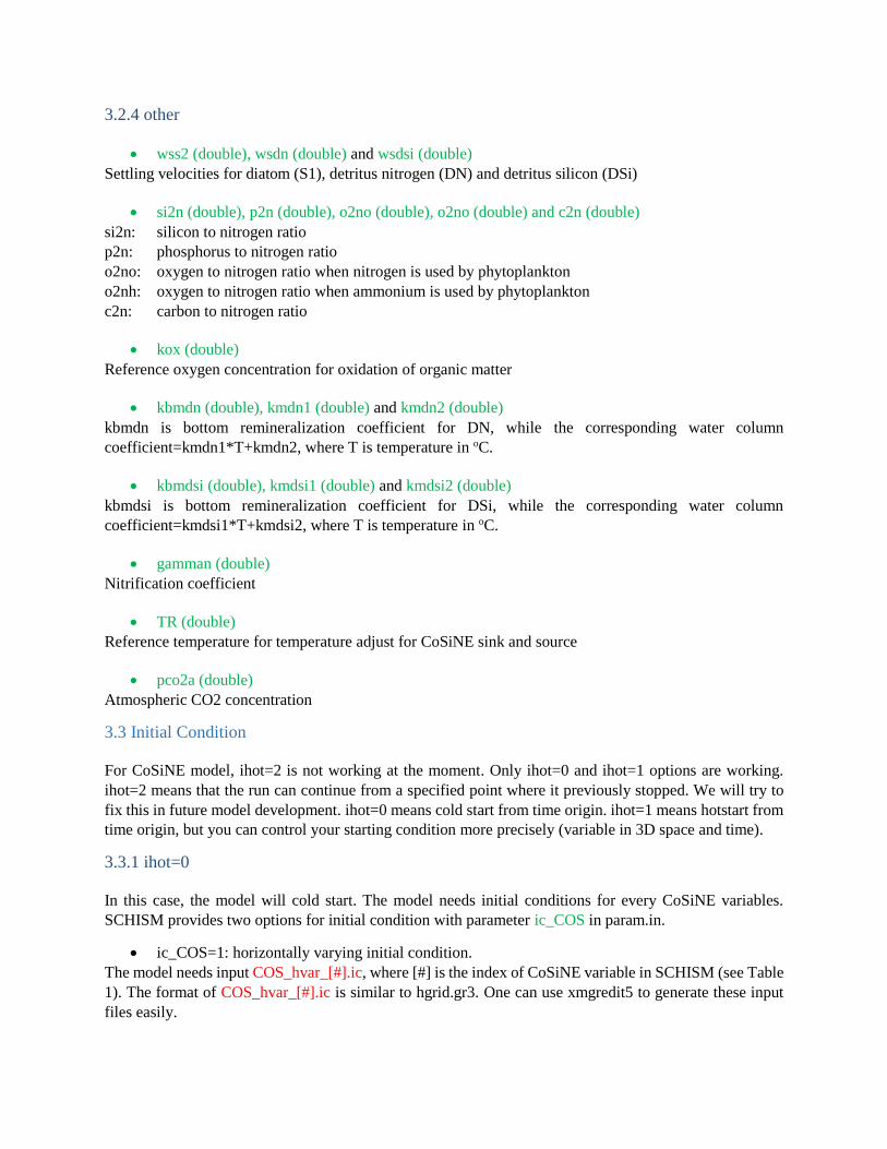
3.2.4 other

wss2 (double), wsdn (double) and wsdsi (double)

Settling velocities for diatom (S1), detritus nitrogen (DN) and detritus silicon (DSi)

si2n (double), p2n (double), o2no (double), o2no (double) and c2n (double)

si2n: silicon to nitrogen ratio

p2n: phosphorus to nitrogen ratio

o2no: oxygen to nitrogen ratio when nitrogen is used by phytoplankton

o2nh: oxygen to nitrogen ratio when ammonium is used by phytoplankton

c2n: carbon to nitrogen ratio

kox (double)

Reference oxygen concentration for oxidation of organic matter

kbmdn (double), kmdn1 (double) and kmdn2 (double)

kbmdn is bottom remineralization coefficient for DN, while the corresponding water column

coefficient=kmdn1*T+kmdn2, where T is temperature in oC.

kbmdsi (double), kmdsi1 (double) and kmdsi2 (double)

kbmdsi is bottom remineralization coefficient for DSi, while the corresponding water column

coefficient=kmdsi1*T+kmdsi2, where T is temperature in oC.

gamman (double)

Nitrification coefficient

TR (double)

Reference temperature for temperature adjust for CoSiNE sink and source

pco2a (double)

Atmospheric CO2 concentration

3.3 Initial Condition

For CoSiNE model, ihot=2 is not working at the moment. Only ihot=0 and ihot=1 options are working.

ihot=2 means that the run can continue from a specified point where it previously stopped. We will try to

fix this in future model development. ihot=0 means cold start from time origin. ihot=1 means hotstart from

time origin, but you can control your starting condition more precisely (variable in 3D space and time).

3.3.1 ihot=0

In this case, the model will cold start. The model needs initial conditions for every CoSiNE variables.

SCHISM provides two options for initial condition with parameter ic_COS in param.in.

ic_COS=1: horizontally varying initial condition.

The model needs input COS_hvar_[#].ic, where [#] is the index of CoSiNE variable in SCHISM (see Table

1). The format of COS_hvar_[#].ic is similar to hgrid.gr3. One can use xmgredit5 to generate these input

files easily.

ic_COS=2: vertically varying initial condition.

The model needs input COS_vvar_[#].ic, where [#] is the index of CoSiNE variable in SCHISM (see Table

1). The format of COS_vvar_[#].ic is similar to ts.ic (for salinity and temperature). It has the following

format.

43 ! total # of vertical levels

1 -200.0 3.0 !level#, z-coordinate, tracer concentration

1 -100.0 1.0

…..

COS_hvar_[#].ic or COS_vvar_[#].ic are also needed if ihot/=0, but the values in these files are not used

in this case. Instead, the values from hotstart.in will replace them.

3.3.2 ihot=1 or ihot=2

In either of the cases, the model will need input file hotstart.in. It is a binary file and one can refer to

trunk/src/Utility/Gen_Hotstart/ for its format and how to generate this file. It basically contains all state

variables at node/side/element, but now includes concentrations of the 13 CoSiNE variables. With this

option, one can design a generic initial condition for CoSiNE model.

3.4 Boundary Condition

The type of boundary condition of CoSiNE is defined in bctides.in. Consult SCHISM manual to understand

its format. Below is an example for CoSiNE boundary condition (in green).

01/01/2011 00:00:00 PST

0 40. ntip

0 nbfr

5 nope

82 4 -4 4 4 4 ! # of ocean boundary nodes, flags for elevation, velocity, temperature, salinity and CoSiNE

0.3 0.5 !Vel

0.9 !relax.for T

0.9

0.9 !relax for CoSiNE

3 0 1 1 1 1 !Coyote

1. !T

1. !S

1. !relax for CoSiNE

6 0 1 1 1 1 !SJR

1. !T

1. !S

1. !relax for CoSiNE

For CoSiNE model as for all SCHISM modules, there are 5 types (itrtype) of boundary conditions for each

boundary segment. For itrtype>0, a relaxation constants between [0,1] must be specified for inflow

condition.

itrtype=0

No boundary condition is specified

itrtype=1

Time history of CoSiNE Model variables. In this case, the run needs inputs COS_[#].th, where [#] is the

tracer number from 1 to 13. The format is the same as TEM_1.th (see SCHISM manual). These are ASCII

files. Basically, the first column is time stamp, and the rest correspond to time histories of tracer

concentration at each open boundary segment that has itrtype=1. This boundary condition is often used for

river boundary where it is mostly well mixed.

itrtype=2

Constant concentrations are used for the particular boundary segment. You only need to specify 13

concentrations in bctides.in.

itrtype=3

CoSiNE boundary condition is nudged to initial concentration. No additional inputs are required.

itrtype=4

The run needs COS_3D.th. This is a binary file and has similar structure with other *3D.th files. The format

is shown elow

do it=1, nt !all time steps

read(12, rec=it) time, (((trbc(m,k,i), m=1,13), k=1,nvrt), i=1, nodes) !tracers #, layer, nodes

enddo

In COS_3D.th, the variable concentrations for each node at each layer are specified. This type of boundary

condition is often used in open ocean boundary where vertical structures exist. Note that the variable

concentrations specified in this file are only used under inflow conditions; under outflow condition, the

boundary condition is not required. In some cases, you may want to impose certain values around the

boundary that are not influenced by inflow/outflow conditions. For such cases, the tracers nudging option

can be used. To apply this condition, you can set inu_COS=2 in param.in and assign a time step step_nu_tr.

Additionally, prepare input files COS_nu.in and COS_nudge.gr3 in a similar way as to T,S. Under this

circumstance, the boundary condition can be actually omitted. Basically, the COS_nu.in provides the model

all of the tracer concentrations in space and time, while COS_nudge.gr3 specifies the nudging strength

between [0, 1] in the horizontal domain.

3.5 Loading

The CoSiNE loading is added through the source/sink function of SCHISM. Here, the loading at certain

location (element) is regarded as a certain volume of water (m3/s) associated with tracer concentrations. In

SCHISM, this volume of water is treated as a point source/sink. In order to add all of the loadings, you need

to specify the loading locations (elements) in file source_sink.in based on judgement. For example, a

WWTP loading can be treated as a point source and can be placed in the nearest elements. In another

example, if the loading is from a broad watershed, one may want to split the total watershed loading into a

series of (land boundary) elements in proximity to the watershed. The flow (water volume) rates are

specified in file vsource.th, which gives the time histories of flow rates into the corresponding elements.

The tracer concentrations are specified in msource.th. Basically, it provides the time histories of every

variables (including temperature and salinity) for each source/sink. The format of source_sink.in, vsource.th

and msource.th can be found in SCHISM manual. Please note in msource.th, the time histories of

temperature and salinity are also needed. The order is Temperature, Salinity followed by CoSiNE variables.

4 Model Kinetics

This part is to summarize the model kinetics of each variable. The writing is based on the reference (Chai,

Dugdale et al. 2002, Liu;, Chai; et al. 2017). For each variable C inside the model, there are physical

processes including advection and diffusion and biological processes that influence its variation. It can be

expressed in the following equation

)(biology)(Physics CCt

C

(1)

The physical part is performed in SCHISM code, while the biological part is done in CoSiNE model. The

following are the mass balance equations for the biological kinetics of each state variable, and we’ll omit

the Physic (C) part.

2.1 Phytoplankton: S1 and S2

There are two phytoplankton species: small phytoplankton and diatom. The growth is the only source term

(NPS# is for nitrate uptake and RPS# is for ammonium uptake), while the sink terms include grazing and

mortality. In addition, there is another sink term related to settling of diatom.

11111

1 SGRPSNPSt

Ss

(2)

z

SwssSGRPSNPS

t

Ss

222222

22 (3)

111311 max SPSfNONPS (4)

1114,414

4*1max11 max SPSfNH

NHsknh

NHknsRPS

(5)

222322 max SPSfNONPS (6)

2224,424

4*2max22 max SPSfNH

NHsknh

NHknsRPS

(7)

1413

1312,14,1413min13

SbfNHSbfNO

SbfNOSfCOSfPOSbfNHSbfNOSfNO

(8)

1413

1412,14,1413min14

SbfNHSbfNO

SbfNHSfCOSfPOSbfNHSbfNOSfNH

(9)

2423

2322,24,24,2423min23

SbfNHSbfNO

SbfNOSfCOSfPOSfSiOSbfNHSbfNOSfNO

(10)

2423

2422,24,24,2423min24

SbfNHSbfNO

SbfNHSfCOSfPOSfSiOSbfNHSbfNOSfNH

(11)

212

22,

414

414

COskco

COfCO

POskpo

POSfPO

(12)

222

22,

424

424,

424

424

COskco

COfCO

POskpo

POSfPO

SiOsksio

SiOSfSiO

(13)

13

314

14

4113

31413

skno

NOspnh

sknh

NHskno

NOspnhSbfNO

(14)

13

314

14

4114

414

skno

NOspnh

sknh

NHsknh

NHSbfNH

(15)

23

324

24

4123

32423

skno

NOspnh

sknh

NHskno

NOspnhSbFNO

(16)

23

324

24

4124

414

skno

NOspnh

sknh

NHsknh

NHSbfNH

(17)

1.0,1min1441

NHespnh

(18)

1.0,1min2442

NHespnh

(19)

II

eeP max1max1

1

11

(20)

II

eeP max2max2

2

12

(21)

0

3

0

2 )21(

0hh

1 dzSPMkdzSSkZk

eII (22)

111

111 max Z

Skgz

SGG

(23)

ptkgz

tZtStSGtG

2

)7d(2)7d(2)7d(22)(2 1

max (24)

)7()7(1)7(2 321 dtDNdtZdtSt (25)

)7()7()7(1)7(1)7(2)7(2 321 dtDNdtDNdtZdtZdtSdtSp (26)

NPS1: nitrate uptake by microzooplankton (mmol m-3 day-1)

RPS1: ammonium uptake by microzooplankton (mmol m-3 day-1)

NPS2: nitrate uptake by mesozooplankton (mmol m-3 day-1)

RPS2: ammonium uptake by mesozooplankton (mmol m-3 day-1)

fNO3S1: nitrate limiting function for small phytoplankton

fNH4S1: ammonium limiting function for small phytoplankton

fPO4S1: phosphate limiting function for small phytoplankton

fCO2S1: carbon limiting function for small phytoplankton

fNO3S2: nitrate limiting function for diatom

fNH4S2: ammonium limiting function for diatom

fSiO4S2: silicate limiting function for small diatom

fPO4S2: phosphate limiting function for small diatom

fCO2S2: carbon limiting function for small diatom

bfNO3S1: nitrate limiting function for small phytoplankton before adjustment

bfNH4S1: ammonium limiting function for small phytoplankton before adjustment

bfNO3S2: nitrate limiting function for diatom before adjustment

bfNH4S2: ammonium limiting function for diatom before adjustment

G1: grazing on small phytoplankton by microzooplankton (mmol m-3 day-1)

G2: grazing on diatom by mesozooplankton (mmol m-3 day-1)

γs1: mortality rate for small phytoplankton (day-1)

γs2: mortality rate for diatom (day-1)

wss2: settling velocity of diatom (m day-1)

μ1max: maximum growth rate of small phytoplankton (day-1)

μ2max: maximum growth rate of diatom (day-1)

kns1: nighttime ammonium uptake for small phytoplankton

kns2: nighttime ammonium uptake for diatom

pnh4s1: ammonium inhibition factor for small phytoplankton

pnh4s2: ammonium inhibition factor for diatom

P1: photosynthetic rate for small phytoplankton at a given light intensity

P2: photosynthetic rate for diatom at a given light intensity

kno3s1: reference nitrate concentration for small phytoplankton growth (mmol m-3)

knh4s1: reference ammonium concentration for small phytoplankton growth (mmol m-3)

kno3s2: reference nitrate concentration for diatom growth (mmol m-3)

knh4s2: reference ammonium concentration for diatom growth (mmol m-3)

ψ1: ammonium inhibition factor for small phytoplankton (mmol-1 m3)

ψ2: ammonium inhibition factor for diatom (mmol-1 m3)

α1: the initial slope of P-I curve for small phytoplankton (unit?)

α2: the initial slope of P-I curve for diatom (unit?)

β: the slope for photo-inhibition (unit?)

I: light intensity (unit?, w/m2)

I0: light intensity at water surface (unit?)

k1: background light extinction coefficient (m-1)

k2: light extinction coefficient due to phytoplankton (mmol-1 m2)

k3: light extinction coefficient due to suspended particulate matter (g-1 m2)

SPM: the concentration of suspended particulate matter (mg/L)

G1max: maximum grazing rate of microzooplankton on small phytoplankton (day-1)

G2max: maximum grazing rate of mesozooplankton on small phytoplankton (day-1)

kgz1: reference concentration of small phytoplankton for microzooplankton grazing (mmol m-3)

kgz2: reference concentration for mesozooplankton grazing (mmol m-3)

ρ1, ρ2, ρ3: mesozooplankton grazing preference factors

ρ8, ρ9: immediate variables for mesozooplankton grazing

t: time (day)

t-7d: refer to variable concentration 7 days earlier (day)

z: depth (m)

h: water depth (m)

2.2 Zooplankton: Z1 and Z2

There are two zooplankton groups: microzooplankton (Z1) and mesozooplankton (Z2). Grazing is the only

source term for zooplankton, while sink terms includes zooplankton excretion and mortality. In addition,

there is another sink term for microzooplankton, that is, predation by mesozooplankton.

2

1 131111

ZGZkOXRGt

Zzex

(27)

2

2 2224322

ZZkOXRGGGt

Zzex

(28)

ptkgz

tZtZtZGtG

2

)7d(2)7d(1)7d(12)(3 2

max (29)

ptkgz

tZtDNtDNGtG

2

)7d(2)7d()7d(2)(4 3

max (30)

columnwaterfor,

bottomfor,1

DOXkox

DOXOXR (31)

γ1: assimilation rate for microzooplankton

γ2: assimilation rate for mesozooplankton

γz: specific mortality rate of microzooplankton and mesozooplankton

k1ex: microzooplankton excretion rate (day-1)

k2ex: mesozooplankton excretion rate (day-1)

G3: grazing on microzooplankton by mesozooplankton (mmol m-3 day-1)

G4: grazing on detritus nitrogen by mesozooplankton (mmol m-3 day-1)

OXR: oxidation rate of organic matter

kox: half saturation constant of dissolved oxygen for oxidation (mmol m-3)

2.3 Dissolved Nutrients: NO3, NH4, SiO4 and PO4

There are four dissolved nutrient forms: nitrate, ammonium, silicate and phosphate. For nitrate, the source

term is the nitrification from ammonium, while the sink term is phytoplankton uptake. For ammonium, the

source terms include zooplankton excretion and remineralization of detritus nitrogen, while the sink terms

include phytoplankton uptake and nitrification. For silicate, the source term is remineralization from detritus

silicon, while the sink term is phytoplankton uptake. For phosphate, the source terms include zooplankton

excretion and remineralization from detritus phosphorus, while the sink term is phytoplankton uptake.

NitOXRNPSNPSt

NO

21

3 (32)

MIDNOXRZOXRZkOXRNitOXRRPSRPSt

NHexex

22k1121

4 (33)

MIDSInsiRPSNPSt

SiO

2*)22(

4 (34)

npMIDNOXR

npZkZOXRnpRPSNPSRPSNPSt

POex

2*

2221k1222114

ex

(35)

4NHNit n (36)

columnwaterfor,2*1

bottomfor,*

DNkmTkm

DNkbmMIDN

DNDN

DN (37)

columnwaterfor,2*1

bottomfor,*

DSIkmTkm

DSIkbmMIDSI

DSiDSi

DSi

(38)

Nit: nitrification from ammonium to Nitrate (mmol m-3 day-1)

γn: nitrification rate (day-1)

si2n: silicon to nitrogen ratio

p2n: phosphorus to nitrogen ratio

MIDN: remineralization of detritus nitrogen (mmol m-3 day-1)

MIDSI: remineralization of detritus silicon (mmol m-3 day-1)

kbmDN: remineralization coefficient for bottom detritus nitrogen (day-1)

km1DN: temperature dependence remineralization coefficient for water column detritus nitrogen (day-1 oC-

1)

km2DN: minimum remineralization coefficient for water column detritus nitrogen (day-1 oC-1)

kbmDSi: remineralization coefficient for bottom detritus silicon (day-1)

km1DSi: temperature dependence remineralization coefficient for water column detritus silicon (day-1 oC-1)

km2DSi: minimum remineralization coefficient for water column detritus silicon (day-1 oC-1)

T: temperature (oC)

2.4 Detritus Organic Matter: DN and DSI

There are two detritus species: detritus nitrogen and detritus silicon. For detritus nitrogen, the source terms

include zooplankton grazing, phytoplankton and zooplankton mortality, while the sink terms include

mesozooplankton grazing, remineralization and settling. For detritus silicon, the source terms include

mesozooplankton grazing on diatom and diatom mortality, while the sink terms include remineralization

and settling.

z

DNwsdnZZMIDNOXR

SSGGGGGt

DN

zz

ss

22

2121

21

214432111

(39)

z

DSiwsdsiMIDSInsiSG

t

DSis

222 2 (40)

wsd: settling velocity of detritus nitrogen (m day-1)

wsdsi: settling velocity of detritus silicon (m day-1)

2.5 Oxygen and Carbon System: DOX, CO2, and ALK

For dissolved oxygen, the source term is phytoplankton photosynthesis, while the sink terms include

nitrification, zooplankton excretion and remineralization. For total carbon dioxide, the source terms include

zooplankton excretion and remineralization, while the sink term is phytoplankton photosynthesis. In

addition, there is air-sea exchange for dissolved oxygen and total carbon dioxide. For total alkalinity, the

source terms include nitrate uptake by phytoplankton, zooplankton excretion and remineralization from

detritus nitrogen, while the sink terms include ammonium uptake by phytoplankton and nitrification.

z

flxoMIDNOXRnhoZkZkOXR

NitOXRnhoRPSRPSnooNPSNPSt

DOX

exex

222211

2221221

(41)

z

flxcoMIDNOXR

ncZkZkOXRncRPSNPSRPSNPSt

COexex

2

22211222112

(42)

MIDNOXRZkZkOXR

NitOXRRPSRPSNPSNPS

t

NH

t

NO

t

ALK

exex

2211

22121

43

(43)

o2no: oxygen to nitrogen ratio when nitrogen is used by phytoplankton

o2nh: oxygen to nitrogen ratio when ammonium is used by phytoplankton

c2n: carbon to nitrogen ratio

o2flx: oxygen flux through reaeration (mmol m-2 day-1)

co2flx: carbon dioxide flux through reaeration (mmol m-2 day-1)

Δz: surface layer thickness (m)

2.6 Temperature Adjustment

Temperature is assumed to influence the reaction terms of all CoSiNE variables. The Q10 function is applied.

It modifies all the reaction terms and the reference temperature is specified by parameter TR mentioned

above.

)(069.0

10

TRTeQ (44)

References

Chai, F., R. C. Dugdale, T. H. Peng, F. P. Wilkerson and R. T. Barber (2002). "One-dimensional ecosystem

model of the equatorial Pacific upwelling system. Part I: model development and silicon and

nitrogen cycle." Deep-Sea Research Part Ii-Topical Studies in Oceanography 49(13-14): 2713-

2745.

Chai, F., M. S. Jiang, R. T. Barber, R. C. Dugdale and Y. Chao (2003). "Interdecadal variation of the

transition zone chlorophyll front: A physical-biological model simulation between 1960 and 1990."

Journal of Oceanography 59(4): 461-475.

Chai, F., M. S. Jiang, Y. Chao, R. C. Dugdale, F. Chavez and R. T. Barber (2007). "Modeling responses of

diatom productivity and biogenic silica export to iron enrichment in the equatorial Pacific Ocean."

Global Biogeochemical Cycles 21(3): 16.

Liu;, Q., F. Chai;, R. Dugdale;, Y. Chao;, H. Xue;, S. Rao;, F. Wilkerson; and Y. Zhang (2017). "Modeling

San Francisco Bay Nutrients and Plankton Dynamics." Journal of Estuarine, Coastal and Shelf

Science.