Corrosion Control Study – Desktop Study Revised Draft Report

CITY OF TORRANCE

Corrosion Control Study – Desktop Study ― Revised Draft Report ―

November 2016

AQUAlity Engineering, Inc.

145 Bonita Street, #E, Arcadia, California 91006 Phone (714) 488-0496, www.AQUAlityeng.com

Trussell Technologies, Inc.

232 North Lake Ave, #300, Pasadena, California 91101 Phone (626) 486-0560, www.trusselltech.com

ii

City of Torrance Corrosion Control Study – Desktop Study

― Revised Draft Report ― TABLE OF CONTENTS

Pages Executive Summary ................................................................................................................................................................ 1 1. Introduction ................................................................................................................................................................ ....... 4

1.1. Summary Information on Corrosion and Aggressiveness................................................................... 5 2. Regulatory Requirements ............................................................................................................................................ 5

2.1. Lead and Copper Rule ........................................................................................................................................ 5 2.2. Corrosion Control Study .................................................................................................................................... 6 2.3. DDW’s Requirements for the City.................................................................................................................. 6 2.4. Reporting Requirements for the City ........................................................................................................... 8

3. Water System of the City .............................................................................................................................................. 9 3.1. Water Sources ........................................................................................................................................................ 9 3.2. Distribution System ........................................................................................................................................... 12

4. Corrosion and Aggressiveness of the City’s Water Sources ......................................................................... 12 4.1. Customer Complaints ....................................................................................................................................... 12 4.2. Lead and Copper at Customer Taps ............................................................................................................ 17

4.2.1. Lead ................................................................................................................................................................ 17 4.2.2. Copper ........................................................................................................................................................... 20

4.3. Water Quality in the City’s Water System ................................................................................................ 20 4.3.1. pH .................................................................................................................................................................... 22 4.3.2. Alkalinity ...................................................................................................................................................... 25 4.3.3. Dissolved Inorganic Carbon ................................................................................................................. 29 4.3.4. Manganese and Iron ................................................................................................................................ 32 4.3.5. Orthophosphates ...................................................................................................................................... 35 4.3.6. Other Water Quality Parameters ....................................................................................................... 39

4.4. Indices of Corrosion and Aggressiveness in the City’s Water Sources......................................... 44 4.4.1. Desalter ......................................................................................................................................................... 45 4.4.2. Well 9 ............................................................................................................................................................. 47 4.4.3. Wells 10, 12 and 13.................................................................................................................................. 48 4.4.4. MWD .............................................................................................................................................................. 49 4.4.5. Comparison of All Water Sources ...................................................................................................... 50

5. Corrosion Control Strategies for the City’s Water System............................................................................ 54 5.1. Recommended Corrosion Control Strategies for the City ................................................................. 55 5.2. Secondary Effects ............................................................................................................................................... 56

6. Bench and Pilot Tests ................................................................................................................................................... 57 6.1. Bench-scale Tests ............................................................................................................................................... 57 6.2. Pilot-scale Tests .................................................................................................................................................. 59

6.2.1. Monitoring Associated with the Pipe Racks .................................................................................. 60 7. Recommendations and Next Steps ......................................................................................................................... 61 8. References and Additional Reading ....................................................................................................................... 62

iii

APPENDIX A: Background on Corrosion and Aggressiveness …………………………………………………..… 64 APPENDIX B: Background on Corrosion Control Strategies …………………………………………..…………… 72 APPENDIX C: Water Quality Data at MWD Turnouts …………………………………….………………….………… 77 LIST OF TABLES

Page Table ES.1: Summary of Water Quality at the Entry Points of the Distribution System ............................ 3 Table 1: CCS Requirements and Proposed Responses for the City ..................................................................... 7 Table 2: Optimal WQPs Recommended by DDW for the City ............................................................................... 8 Table 3: Capacity of the City’s Water Sources.............................................................................................................. 9 Table 4: Pipe Materials Present in the City’s Distribution System .................................................................... 13 Table 5: Customer Complaints that Could Pertain to Corrosion or Aggressiveness ................................. 14 Table 6: Lead Concentrations (mg/L) Measured at the City’s Customer Taps ............................................ 18 Table 7: Copper Concentrations (mg/L) Measured at the City’s Customer Taps ....................................... 21 Table 8: pH Values Measured from the Pilot Boreholes of Wells 10, 12 and 13 ......................................... 23 Table 9: Alkalinity Measured from the Pilot Boreholes of Wells 10, 12 and 13 .......................................... 27 Table 10: DIC Concentrations Calculated from the Pilot Boreholes of Wells 10, 12 and 13 .................. 31 Table 11: Manganese and Iron Concentrations Measured from the Pilot Boreholes

of Wells 10, 12 and 13 .......................................................................................................................................... 34 Table 12: Total Hardness, Calcium, Total Alkalinity, Chloride, Sulfate and TDS Concentrations ........ 42 Table 13: Indices of Aggressiveness and Corrosion Calculated in Watter Pumped

from the Pilot Boreholes of Wells 10, 12 and 13 ...................................................................................... 49 Table 14: Summary of Indices of Corrosion and Aggressiveness for the City’s Water Sources ............ 53 Table 15: Challenges of the Main Corrosion Control Treatments ..................................................................... 58 Table 16: Guidelines for Evaluating Coupon Corrosion Rates ............................................................................ 60 Table A.1: Definitions of Indices of Corrosion and Aggressiveness .................................................................. 70 Table B.1: Chemical Processes Used to Adjust Alkalinity and pH ..................................................................... 74 LIST OF FIGURES

Page Figure 1: Water Sources of the City................................................................................................................................ 10 Figure 2: Customer Complaints Potentially Related to Water Corrosion or Aggressiveness ................ 16 Figure 3: Customer Taps Where Lead Concentrations Exceeded 0.005 mg/L (AL of 0.015 mg/L) .... 19 Figure 4: pH Measured at the Desalter’s Entry Point of the Distribution System ...................................... 22 Figure 5: pH Measured at Well 9 Entry Point of the Distribution System ..................................................... 23 Figure 6: pH Measured at MWD Turnouts .................................................................................................................. 24 Figure 7: pH Measured at the Distribution System Sampling Sites .................................................................. 25 Figure 8: Distribution System Sampling Sites for WQPs ....................................................................................... 26 Figure 9: Total Alkalinity Measured at the Effluents of MWD’s Weymouth,

Diemer and Jensen WTPs ................................................................................................................................... 28 Figure 10: Total Alkalinity Measured at the Distribution System Sites .......................................................... 29 Figure 11: DIC Concentrations at the Effluents of MWD’s Weymouth, Diemer and Jensen WTPs ...... 31 Figure 12: Manganese Concentrations in Desalter Treated Water ................................................................... 32 Figure 13: Manganese Concentrations and Running Annual Averages at Well 9 ....................................... 33 Figure 14: Orthophosphate Concentrations Measured at the Desalter

Distribution System Entry Point ..................................................................................................................... 35

iv

Figure 15: Orthophosphate Concentrations Measured at Well 9 Entry Point of the Distribution System ................................................................................................................................. 36

Figure 16: Orthophosphate Concentrations Measured at MWD Turnouts ................................................... 36 Figure 17: Orthophosphate Concentrations Measured at the Distribution System Sites ....................... 37 Figure 18: Orthophosphate Concentrations Measured in the Distribution System

Between January 2014 and March 2016 ...................................................................................................... 38 Figure 19: Alkalinity and Orthophosphate Measured at Distribution System Sites Nos. 1 and 9 ........ 40 Figure 20: Alkalinity and Orthophosphate Measured at Distribution System Sites Nos. 10 and 11 .. 41 Figure 21: TDS Concentrations Measured in the Desalter Treated Water .................................................... 43 Figure 22: Chloride and Sulfate Concentrations Measured in the Desalter Treated Water ................... 43 Figure 23: Indices of Aggressiveness for the Desalter Treated Water ............................................................ 46 Figure 24: Indices of Corrosion for the Desalter Treated Water ....................................................................... 46 Figure 25: Indices of Aggressiveness of Water Pumped from Well 9 .............................................................. 47 Figure 26: Indices of Corrosion of Water Pumper from Well 9 .......................................................................... 48 Figure 27: Indices of Aggressiveness of MWD Treated Water ........................................................................... 51 Figure 28: Indices of Corrosiveness of MWD Treated Water .............................................................................. 52 Figure 29: Treatment for Lead and/or Copper with Iron and Manganese and pH ≥ 7.2 ......................... 55 Figure 30: Left: Example of Pipe Racks With Two Coupons;

Right: Example of Mild Steel Coupon After Several Weeks of Exposure ........................................ 60 Figure B.1: Conceptual Framework for Corrosion Control Approaches ......................................................... 74 Figure C.1: pH Measured at MWD T-1 and MWD T-6 Turnouts ......................................................................... 78 Figure C.2: pH Measured at MWD T-5 / T-7 and MWD T-8 Turnouts ............................................................. 79 Figure C.3: Orthophosphate Concentrations Measured at MWD T-1 and MWD T-6 Turnouts............. 80 Figure C.4: Orthophosphate Concentrations Measured at MWD T-5 / T-7 and MWD T-8 Turnouts . 81

1


― Revised Draft Report ―

EXECUTIVE SUMMARY

The City of Torrance (City) was mandated by the Division of Drinking Water (DDW) to conduct a corrosion control study (CCS) of its potable water system. This study is required because the City has not completed a system-wide study yet, and the corrosion control treatment currently used may not be optimum with regards to the City’s water quality and distribution condition. The City has been using a 70:30 blend of poly- and ortho-phosphates at the Robert W. Goldsworthy Desalination Plant (Desalter), and a 50:50 blend of poly- and ortho-phosphates at Well 9. Water received from the Metropolitan Water District of Southern California (MWD) does not contain a corrosion inhibitor. Also, the City will soon start using water from new groundwater wells: two new wells will be used to supply the Desalter (i.e., CY Shallow and DP Middle), and Wells 10, 11, 12 and 13 will soon be placed in service. These new water sources offer an opportunity for the City to ensure that it is using the most suitable corrosion control treatment(s).

This report focuses on the first part of the CCS, i.e., the desktop study, and aims at meeting the requirements of the Lead and Copper Rule (LCR). This desktop study assessed the corrosiveness and aggressiveness of the City’s water in light of distribution system materials, evaluated water quality parameters related to corrosion and aggressiveness, examined lead and copper data and customer complaints, assessed the suitability of the current corrosion control treatments that are being used by the City to meet the LCR requirements, and identified alternative corrosion control strategies (as needed) to limit water corrosiveness and metal release. This report includes three appendices that present background information on corrosion and aggressiveness, general approaches to corrosion control treatment, and additional water quality data.

The selection of the most suitable corrosion control treatments for the City’s water sources were derived from observations made during this project, and from the water quality data measured at the entry points and in the City’s distribution system (the water quality parameters that are most closely related to corrosion and aggressiveness are summarized in Table ES.1):

• Both lead and copper have been present at customer taps throughout the City’s distribution system. At certain taps, lead was present above its action level (AL), and copper has been present at low concentrations at many taps. The corrosion indices also suggest that the City’s water sources are corrosive towards metals, but with significant variations between the different pipe materials (i.e., lead and copper, as well as iron). Increasing the orthophosphate dose from 0.2-0.3 mg/L as P in 2011 to its current target of 1.0 mg/L in Desalter treated water and water pumped from Well 9 may have contributed to decreases in lead and copper release at customer taps. These trends suggest that an orthophosphate-containing corrosion inhibitor is beneficial to prevent release of these metals in the City’s water.

2

• Alkalinity and DIC concentrations are low in the Desalter treated water, concentrations are high in water pumped from Well 9 and the pilot boreholes of Wells 10, 12 and 13, and alkalinity and DIC concentrations are moderate in water supplied by MWD. Distributing water with such different water quality can trigger corrosion and destabilize scales present on the inner pipe walls, which can be exacerbated by the fact that the City uses different corrosion control strategies for its water sources. The possibility to harmonize the corrosion control treatments should be examined in bench and pilot testing.

• Hardness and calcium concentrations are high in certain water sources (e.g., Well 9, the new Wells 10 and 12, and some of MWD water supplies), consistent with trends observed with the indices of aggressiveness. This suggest that adjusting alkalinity and pH to increase precipitation of calcium carbonate (CaCO3) may create scaling inside distribution system pipes and customers’ water systems. Moreover, increasing pH beyond its current range would impair orthophosphate efficacy.

• Manganese is present in Desalter treated water, in water pumped by Well 9, and in the pilot boreholes of Wells 10, 12 and 13. The new wells also contain low concentrations of iron. The presence of these metals needs to be considered in the selection of suitable corrosion inhibitors, along with the fact that DDW does not recognize sequestration as an acceptable removal treatment for iron and manganese.

Based on these observations, corrosion inhibitors are recommended for the City’s water sources. However the first task for the City is to identify the wells that will be favored to supply the Desalter, the zones that will be developed in the new Wells 10, 12 and 13, and how it will address the presence of manganese in Well 9. More up-to-date water quality data are also needed from the new wells after they are placed in service. These new data and information should be use to review this report, further narrow down the most suitable corrosion inhibitor(s) for the City’s water sources, and develop the experimental plans for the bench and pilot tests.

3

Table ES.1: Summary of Water Quality at the Entry Points of the Distribution System

Desalter Well 9 Well 10 (1) Well 12 (2) Well 13 (3) MWD (4) pH 7.5 to 8.7;

average of 7.9 7.7 to 8.4;

average of 8.0 8.0 7.6 to 7.7 7.4 to 7.6 8.0 to 8.1 in CRW (5);

8.1 to 8.4 in SPW (6) Alkalinity (mg/L CaCO3)

32 to 37 (7); 50 (8)

180 to 200 (9) 200 to 210 202 to 281 182 to 204 121 to 131 in CRW; 87 to 95 in SPW)

DIC (mg/L as C) 12.2 to 12.7 (10) 43.8 to 51.0 (9) 49 to 51 50 to 70 47 to 51 29 to 32 in CRW; 21 to 23 in SPW

Total hardness (mg/L CaCO3)

Not provided 300 to 335 130 to 160 68 to 300 110 to 120 292 to 306 in CRW; 124 to 136 in SPW

Calcium (mg/L as Ca)

40 to 41 (7, 8) 80 to 90 29 to 42 26 to 136 27 to 33 73 to 80 in CRW; 33 to 37 in SPW

Chloride (mg/L)

120 to 200; average 162

180 to 190 46 to 52 22 to 190 23 to 26 92 to 103 in CRW; 80 to 95 in SPW

Sulfate (mg/L) 34 to 67; average 50

46 to 86 1.1 to 3.1 0.6 to 41 0.7 to 4 237 to 264 in CRW; 98 to 124 in SPW

Manganese (mg/L)

ND (11) to 0.044; average of 0.024

0.050 to 0.058; average of 0.053

0.019 to 0.021 0.015 to 0.040 0.013 to 0.031 Not provided

Iron (mg/L) Not provided, but assumed negligible

< 0.10 0.040 to 0.088 0.052 to 0.134 0.073 to 0.514 Not provided

TDS (12) (mg/L) 280 to 520; average 406

540 to 640 300 to 310 425 to 630 190 to 300 618 to 664 in CRW; 385 to 437 in SPW

(1) Based on a unique sampling conducted in the May 2009 from the pilot borehole, and using only data collected from Zone 1 and Zone 2. (2) Samples were collected on September 11, 12 and 13, 2013 in Zones 1, 2 and 3, respectively. (3) Samples were collected on August 21, 22 and 23, 2013 in Zones 2, 3 and 4, respectively. Data are not presented for Zone 1 because this screen interval was dry. (4) Based on results measured at the Weymouth, Diemer and Jensen Water Treatment Plants effluents between January 2015 and February 2016. (5) SPW: State Project Water. (6) CRW: Colorado River Water. (7) Based on samplings conducted in April 2003 and November 2005. (8) Based on letters received from DDW. (9) Based on samplings conducted in February 2009, January 2011, February 2014 and September 2016. (10) Based on samplings conducted between February 2015 and March 2016. (11) ND: Not detect. (12) TDS: Total dissolved solids.

4


― Revised Draft Report ―

1. INTRODUCTION

The City of Torrance (City) conducted a desktop Corrosion Control Study (CCS) in 1995 and a pilot study in 2005 at the Madrona Well 2, but has not completed a system-wide study yet. Thus the City was mandated by the Division of Drinking Water (DDW) of the State Water Resources Control Board to conduct a CCS of its potable water system because the corrosion control treatment currently used may not be optimum with regards to the City’s water quality and distribution condition. The City is using the following corrosion control treatments for its water sources: Madrona Well 2, which supplies the Robert W. Goldsworthy Desalination Plant (Desalter), uses a 70:30 blend of poly- and ortho-phosphates, Well 9 uses a 50:50 blend of poly- and ortho-phosphates, and water received from the Metropolitan Water District of Southern California (MWD) does not contain a corrosion inhibitor. The City will soon start using water from new groundwater wells: two new wells will be used to supply the Desalter (i.e., CY Shallow and DP Middle), and Wells 10, 11, 12 and 13 will soon be placed in service. In addition to assessing whether the corrosion control treatment that are currently used are adequate, the City needs to determine whether the new wells will require corrosion control, and if so, the most suitable strategy(ies) to implement for these wells.

This CCS report focuses on the first part of the project, i.e., the desktop study, and it aims at meeting the requirements of the Lead and Copper Rule (LCR). This study assessed the corrosiveness and aggressiveness of the City’s water in light of distribution system materials, evaluated other water quality parameters related to corrosion and aggressiveness, examined lead and copper data and customer complaints, assessed the suitability of the current corrosion control treatments that are being used by the City to meet the LCR requirements, and identified alternative corrosion control strategies (as needed) to limit water corrosiveness and metal release. This study emphasized lead and copper corrosion as per the current regulatory requirements, but also addressed additional benefits that can be drawn from corrosion control, including the possibility to limit the degradation of non-metallic pipes.

This report includes background information on corrosion and aggressiveness. For clarity purposes, this information is presented in Appendix A, and a brief summary is shown in Section 1.1. Regulatory requirements are presented in Section 2, including descriptions of the LCR and CCS, and the specific requirements that were required by DDW. Section 3 briefly presents the City’s water system. Section 4 shows all analyses that were conducted during this evaluation. Section 5 discusses the corrosion control strategies that are available to the City based on analyses conducted during this study; this section builds from the background information on corrosion control that is presented in Appendix B. Section 6 describes the bench and pilot tests that will be required to complete this CCS. Recommendations and next steps are presented in Section 7. The main references and documents used during this evaluation are listed in Section 8.

5

1.1. Summary Information on Corrosion and Aggressiveness

Corrosion is an electrochemical interaction between a metal surface (e.g., a pipe wall) and water. While it is important to understand and control corrosion, metal release into the water is the process that drives drinking water regulations, and that may present the greatest risks to public health. Pipe scales that build up on the metal surface are also important, and can include two types of compounds: (1) passivating films that form when pipe material and water react directly with each other; and (2) deposited scale material that forms when substances in the water (e.g., iron, manganese, aluminum, calcium) precipitate or sorb to, and then build up on the pipe surface.

Erosion of pipe internal surfaces and linings is a phenomenon that differs from metal corrosion. It derives from aggressive waters, and mainly affects cement-mortar lined pipes and asbestos-cement pipes. These pipes are composed of various calcium-based compounds that can dissolve in aggressive waters. Appendix A presents detailed information about corrosion and aggressiveness.

Many factors influence corrosion and aggressiveness, sometimes in a conflicting ways. Distribution system materials play an essential role in the process, and water that may be passivating for one material may be corrosive for another. Likewise, many water quality parameters need to be considered when examining the corrosiveness and aggressiveness of a water source, which was the rationale for developing indices of corrosion and aggressiveness, such as the Langelier Saturation Index. Within one distribution system, differences in water sources and treatment strategies may lead to different water quality, which has also promoted corrosion in some systems. Lastly, distribution system hydraulic conditions such as water velocity, water usage and flow direction also influence corrosion and aggressiveness. Appendix A provides detailed information about each of these factors.

2. REGULATORY REQUIREMENTS

This section briefly introduces the LCR, the water quality parameters (WQPs) and the CCS procedures. DDW’s requirements for the City with regards to corrosion control and associated reporting are also presented. From a regulatory perspective, corrosion and its associated monitoring and reporting strictly pertains to lead and copper.

2.1. Lead and Copper Rule

The LCR is presented in Chapter 17.5 of Title 22 of the California Code of Regulations (Division 4 Environmental Health). Recognizing that lead and copper are rarely present in raw water sources but instead come from pipes, materials, fittings and fixtures of premise plumbing (also called “service lines”), the requirements of the LCR include Action Levels (AL) that are based on monitoring at customer taps. The ALs are the following:

• Lead: 90th percentile less than 0.015 mg/L (i.e., no more than 10% of the samples can exceed 0.015 mg/L for lead).

• Copper: 90th percentile less than 1.3 mg/L (i.e., no more than 10% of the samples can exceed 1.3 mg/L for copper).

The number of samples are based on population served. Unless otherwise advised by DDW, samples shall be collected during the months of June, July, August or September. All samples shall be first-

6

draw samples, i.e., each sample shall consists of 1 liter of water that has stood motionless in the plumbing system for at least 6 hours, but not more than 12 hours.

The LCR is a treatment technique rule because AL exceedances do not lead to violations, but they trigger other requirements, which may include implementing corrosion control treatment to decrease lead and copper concentrations at customer taps, source water monitoring and/or treatment, public education, and/or lead service line replacement.

The LCR requires large water systems (i.e., serving more than 50,000 people) to optimize their corrosion control treatment, which includes monitoring for lead and copper at customer taps, and monitor for WQPs for one year to allow DDW to designate an adequate treatment for each system. The WQPs specific monitor for corrosion control may include the following parameters: pH, alkalinity, orthophosphate (when an inhibitor containing a phosphate compound is used), silica (when an inhibitor containing a silicate compound is used), calcium, conductivity and water temperature.

Since its original publication in 1991, the LCR has undergone a number of revisions, and Long-term Revisions of the LCR are now in preparation to further improve public health protection and streamline the rule requirements. The proposed changes will improve the effectiveness of the corrosion control treatment in reducing exposure to lead and copper, and may trigger additional actions to equitably reduce the public’s exposure to lead and copper when corrosion control treatment alone is not effective. The main issues that may be changed include sample site selection criteria, lead sampling protocols, public education for copper, measures to ensure optimal corrosion control treatment, and lead service line replacement. The effectiveness of partial lead service line replacements (PLSLR) in reducing drinking water lead levels has been heavily examined in preparation of the Long-term Revisions of the LCR, and the Science Advisory Board has provided recommendations centered around the following five issues: associations between PLSLR and blood lead levels in children, water sampling data at the tap before and after PLSLR, comparisons between partial and full lead service line replacements, PLSLR techniques, and the impact of galvanic corrosion. A draft Long-term Revisions of the LCR is expected in 2017, and a final rule should be promulgated by the USEPA in 2018 or 2019.

2.2. Corrosion Control Study

DDW has indicated that the City needs to conduct a CCS according to the LCR and Article 5 (Section 64683) of Title 22 of the California Code of Regulations, including both desktop and pilot studies. A CCS includes a number of tasks, as presented in Table 1.

Based on the studies conducted and recommendations made, DDW may either approve the corrosion control treatment option(s) recommended from a CCS, or designate alternative corrosion control treatment(s), or request additional information.

2.3. DDW’s Requirements for the City

The City’s permit amendment of December 19, 2006 pertains to the Madrona Well 2 that supplies the Desalter. It allows the City to treat water that bypasses the Desalter with polyphosphates to sequester manganese. The permit amendment stated that a blend of poly- and ortho-phosphates should be used, and it specifically mentioned LA Chemical product No. LACCO3672, which is a 75:25 blend of poly- and ortho-phosphates. This product was tested in untreated bypass water from Madrona Well 2 during pilot testing conducted between April and September 2005. The maximum concentration allowed by ANSI/NSF Standard 60 is 25 mg/L, and the target dose was 3.85 mg/L as PO43-

7

(i.e., 1.26 mg/L as P) in the bypass water or 0.33 mg/L as PO43- (i.e., 0.11 mg/L as P) in Desalter treated water. The corrosion inhibitor discussed in the December 2006 permit amendment was later changed to a 70:30 blend of poly- and ortho-phosphates distributed by Carus Corporation (product No. 8100).

Table 1: CCS Requirements and Proposed Responses for the City

CCS Requirements City’s Responses

Evaluate the effectiveness of the corrosion control strategies that are available to water systems (described in Appendix B), which include alkalinity and pH adjustment, calcium hardness adjustment, and the addition of a corrosion inhibitor at a concentration sufficient to maintain an effective residual throughout the distribution system.

This task is discussed in this report.

Evaluate suitable corrosion control treatments using either pipe rig/loop tests, metal coupon tests, partial-system tests, or analyses based on documentation of such treatments from systems of similar size, water chemistry and distribution system configuration.

This task will be conducted during the second phase of this project.

Measure the WQPs listed in Section 2.1 before and after evaluating the corrosion control treatments.

The City is currently monitoring for the WQPs requested by DDW, with the exception of calcium.

Identify all chemical or physical constraints that limit or prohibit the use of a particular corrosion control treatment based on results obtained from another water system with comparable water quality characteristics, with supporting documentation.

There are no reports of treatments that cannot be used in the greater Los Angeles area.

Evaluate the effect of the chemicals used for corrosion control treatment on other water treatment processes (i.e., secondary impacts).

Secondary effects of the corrosion control treatment options are discussed in Section 5.2.

Recommend to DDW, in writing, the treatment option that the CCS indicate constitutes corrosion control treatment for the system, on the basis of the data generated and evaluations conducted, with supporting documentation.

This report presents the preliminary recommendations that were made during this desktop study. The subsequent pilot study will confirm these recommendations.

The City’s permit amendment of January 18, 2011 allows the City to distribute water pumped from Well 9. This amendment states that a 50:50 blend of poly- and ortho-phosphates shall be use, and it specifies that Carus Corporation’s product No. 8500 should be used. This particular amendment only mentions the maximum allowable concentration, which is 23 mg/L. The permit amendment of January 2011 emphasizes that although the proposed corrosion inhibitor contains polyphosphate, its sequestering ability does not constitute an acceptable removal treatment for iron and manganese, should the concentrations of these metals exceed the Primary or Secondary Standard (the effect of

8

polyphosphates are described in Section B.2 of Appendix B, and may explain the exclusion of polyphosphates as an acceptable treatment technique for iron and manganese).

DDW’s evaluation of the City’s 2011 lead, copper and WQP monitoring data is presented in its letter of July 9, 2012. Based on this evaluation, DDW proposed the tentative optimal WQPs, which were pH of 7.2 to 8.5 and an orthophosphate residual of at least 0.5 mg/L as P at the entry points of the distribution system for the Desalter and Well 9. These optimal WQPs were revised in DDW’s letter of September 2013, as presented in Table 2. These targets are discussed in Sections 5 and 7. This last letter from DDW includes the following requirements:

“The City is considered out of compliance with the WQP ranges for any period during which it has excursions for more than nine days. When an excursion occurs, within 48 hours of being notified of the results of the initial sample(s), the City must investigate the cause and collect a follow up samples at each affected site for each WQP that did not meet the Department-specified values.”

Table 2: Optimal WQPs Recommended by DDW for the City

Parameter Entry Points of the Desalter and Well 9

In the Distribution System

pH 7.2 – 8.4 7.2 – 8.4

Orthophosphate ≥ 0.5 mg/L as P ≥ 0.5 mg/L as P where alkalinity is < 60 or > 160 mg/L CaCO3

2.4. Reporting Requirements for the City

The City’s permit amendments state that a number of reports need to be submitted to DDW by the 10th of the following month. Only the reports that specifically pertain to corrosion or corrosion protection are listed here:

• A summary of WQPs and orthophosphate testing results (measured in-house and by external laboratories) in the reporting calendar month in water pumped from Madrona Well 2, effluent of the reverse osmosis (RO) membranes prior to and after blending, in water pumped from at Well 9, and throughout the distribution system.

• A summary of the daily operational record, including flow rates and total volume of treated water, daily dosages of corrosion inhibitors, daily minimum and maximum total chlorine residuals at the plant effluents (specific conductance is also required in the Desalter treated water), operation schedule, and operational changes and unusual circumstances, including scheduled interruptions and unscheduled interruptions.

• A summary of the customer complaint records.

9

3. WATER SYSTEM OF THE CITY

The City serves approximately 115,000 people through roughly 26,500 service connections. The City’s water sources and distribution system are described in this section.

3.1. Water Sources

When this report was prepared, the City’s water sources included two active wells and five connections with MWD, and a number of new wells were being commissioned. The City also maintains emergency connections with two neighboring water systems (California Water Service Company – Dominguez, and the City of Lomita). The water sources that are currently used by the City and that are considered in the future are described hereunder. Their capacity is shown in Table 3 and they are illustrated in Figure 1.

Table 3: Capacity of the City’s Water Sources

Water Source Capacity (gpm)

Desalter:

• Madrona Well 2 • CY Shallow • DP Middle

4,200 Unknown Unknown

Well 7

Well 9 3,000

Well 10 2,200 to 2,500 (1)

Well 11 Unknown

Well 12 1,800 to 2,500 (1)

Well 13 1,400 to 1,900 (1)

Well 14 Unknown

MWD T-1 8,977

MWD T-5 2,244

MWD T-6 4,488

MWD T-7 6,732

MWD T-8 11,221 (1) The exact well capacity will be determined once the pumping zones are identified and pumping tests are conducted.

Figure 1: Water Sources of the City 10

11

Desalter: The Robert W. Goldsworthy Desalination Plant (Desalter) is one of the programs of the Water Replenishment District (WRD) of Southern California. The purpose of the Desalter is to treat a saline plume located in the West Coast Basin, and that was trapped as a result of barrier operations designed to halt seawater intrusion. The product water of the Desalter is sold to the City for distribution in its potable water system.

The Desalter has been feed by the Madrona Well 2 until now, but two new wells (i.e., CY Shallow and DP Middle) will be commissioned in 2017 to provide additional water supply to the Desalter.

Following pre-treatment, the Desalter uses RO membranes to remove chloride and decrease total dissolved solids (TDS) concentrations; the treatment goal for TDS is 400 mg/L and 450 μS/cm for conductivity. Until now, the RO permeate was blended with untreated bypassed water from the Madrona Well 2 at a ratio of approximately 20%. Before blending, the bypass water received a 70:30 blend of poly- and ortho-phosphates (product No. 8100 distributed by Carus Corporation). With LA Chemical’s product No. LACCO3672, the City’s permit amendment of December 19, 2006 had proposed a dose of 3.85 mg/L as PO43- (i.e., 1.26 mg/L as P) in the bypass water or 0.33 mg/L as PO43- (i.e., 0.11 mg/L as P) in Desalter treated water. These doses were based on water hardness, and iron and manganese concentrations. The corrosion inhibitor was subsequently changed to a 70:30 blend of poly- and ortho-phosphates distributed by Carus Corporation (product No. 8100) at a target dose of 0.5 mg/L as P or more. After blending, the treated water receives sodium fluoride, and chlorine and ammonia to form monochloramine at a residual of 2.2 mg/L Cl2.

Well 7: Well 7 is a standby well that is used only on an as-needed basis for fire flow demands or other emergencies. Thus it is not discussed further in this document.

Well 9: Well 9 is a replacement well for Well 6. Well 9 received its permit on January 18, 2011. Water pumped from Well 9 receives a 50:50 blend of poly- and ortho-phosphates provided by Carus Corporation (product No. 8500), which contains 35% of total phosphates, i.e., 17.5% of active polyphosphates and 17.5% of active orthophosphates. This compound was selected because it was used at Well 6, and both Wells 6 and 9 have showed similar water quality. The target dose proposed by DDW in its January 2011 letter (i.e., 0.91 mg/L as PO43- or 0.30 mg/L as P) was determined by the manufacturer, and was based on the water’s hardness, and iron and manganese concentrations. DDW’s letter of September 2013 revised the target dose of corrosion inhibitor to 0.5 mg/l as P or more. Immediately after phosphate addition (within a couple of feet downstream, on the same influent pipeline), sodium hypochlorite is dosed to obtain a residual of 2.0 mg/L Cl2. Free chlorinated water is stored in the 1-MG Yukon Tank. The tank inlet allows removal of H2S by aeration. Before distribution, ammonia is added to reach a chlorine-to-ammonia-N ratio of 5:1, and fluoride is added at a dose of 0.6 to 0.8 mg/L.

Manganese concentrations have been fluctuating in water pumped from Well 9, leading to an exceedance of the Secondary Drinking Water Standard for this contaminant in the third quarter of 2014; the running annual average (RAA) was 0.0555 mg/L and the Secondary Standards is 0.05 mg/L. The exceedance was explained in a citation received from DDW in October 2014. First, the City attempted to apply for a waiver, but it is now weighing its option to provide removal treatment for manganese (along with other contaminants) at this wellhead.

Future North Torrance Well Field Project (NTWFP): In the future, the City is planning to treat Well 9 water at the NTWFP, which is located approximately 500 yards from the Well 9 site. The NTWFP will also receive water from the future Well 10 that will be located at the same site. Different scenarios are being considered for water that will be pumped from this well, including: (1) keeping waters from Well 9 and Well 10 separate; (2) blending water from both wells together; (3) blending water from

12

Well 9 with MWD water, or water from Well 10 with MWD water; or (4) blending all three water sources together (Well 9, Well 10, and MWD). The treatment strategy for Well 10 has not been determined yet, but it will receive chlorine and ammonia to reach a chlorine-to-ammonia-N ratio of 5:1. The 1-MG Yukon Tank (a steel tank) that is currently present at the Well 9 site will be removed, and a 3-MG concrete tank will be built at the NTWFP to receive water pumped from Wells 9, 10 and potentially 11.

Only a pilot borehole is available for Well 10 at this time. The well will be drilled in 2017, and is expected to be put in service towards the end of 2018.

Well 11 is not drilled yet. This well may also supply the future NTWFP.

Van Ness Well Field Project: In the northeast part of the City’s service area and adjacent to the Van Ness Avenue, the City is developing a new groundwater project that will add two to three new wells to the City’s water portfolio. Pilot boreholes were drilled for Wells 12 and 13 in August and September 2013. Well 14 may also be developed at a later time.

MWD: Water received from MWD is surface water treated by either one of three treatment plants: Weymouth, Diemer or Jensen Water Treatment Plants (WTPs). At the effluents of these plants, monochloramine is added at a chlorine-to-ammonia-N ratio of 5:1. MWD does not use a corrosion inhibitor, but pH is maintained above 8.0.

3.2. Distribution System

The City’s service area is 16.2 sq. miles, and its distribution system is separated into three pressure zones. It includes three storage tanks with a combined capacity of approximately 29.7 MG and five booster stations. The distribution system is composed of approximately 440 miles of pipes made of various materials, as shown in Table 4. Most of the ductile iron, cast iron and steel pipes are lined. The pipes presented in Table 4 do not include individual service lines (i.e., premise plumbing), which are made of copper pipes for the most part (98 to 99%). The remaining service lines are made of plastic pipes (approximately 1%) or galvanized pipes (less than 1%).

Considering the nature of the distribution system pipes, both corrosion and dissolution of calcium from pipes can occur in the City’s distribution system.

4. CORROSION AND AGGRESSIVENESS OF THE CITY’S WATER SOURCES

This section presents the extent of the corrosion problem in the City’s distribution system, starting with a review of the customer complaints received between October 2014 and April 2016, an analysis of lead and copper sampling results since 2011, an examination of water quality data collected at the entry points of the distribution system and in the system, and an analysis of indices of corrosion and aggressiveness.

4.1. Customer Complaints

Customer complaints received by the City between October 31, 2014 and April 19, 2016, and that could pertain to corrosive or aggressive water were compiled. Results are presented in Table 5, where the orange-pink rows indicated colored-water complaints that could be explained by City staff, the green rows indicate colored-water complaints that could not be explained by City staff, and the non-colored rows indicated complaints that were not related to colored water but could be related

13

Table 4: Pipe Materials Present in the City’s Distribution System

Material Abbreviation Proportion of Distribution System

Asbestos cement AC 7.9%

Ductile iron DI 37%

Cast iron CI 51%

Concrete cylinder pipe CCP 0.20%

Cement mortar-lined concrete CMLC 0.09%

High-density polyethylene HDPE 0.10%

Mortar lined and coated steel ML & CS 2.0%

Polyvinyl chloride PVC <0.01%

Reinforced cement concrete RCC 1.2%

Reinforced concrete pipe RCP 0.77%

Steel STL 0.04%

to corrosion or aggressiveness. Because metal concentrations are not measured when City staff responds to customer complaints, it is not possible to assess the nature of the color-water complaints, particularly for complaints that could not be explained. The complaints are numbered in the left column of Table 5, and these numbers were used to locate the complaint sites, as illustrated in Figure 2. Complaints about tastes or odors, pressure, air in pipes or other situations not related to corrosion were not considered in this evaluation.

A total of 28 complaints that could potentially be related to corrosive or aggressive water were received (complaints received from the same vicinity and for the same reason were grouped together in the same row). Figure 2 indicates that complaints were localized in two specific areas, i.e., Well 9 in the Northern part of the service area, and between the Desalter and the MWD T-8 turnout. Because the area between the Desalter and MWD T-8 is considered the Old Torrance, it is likely that service lines and premise plumbing are older, which may explain some of the complaints received.

Of the 28 complaints analyzed, there were 11 complaints of colored water that were related to either flushing, flow testing, main repair, a street sweeper pulling water from a nearby hydrant, or a broken hydrant. Five (5) complaints were not related to colored water. Of these, two complaints pertained to pinhole leaks in copper pipes, one complaint was related to scaling, and two complaints pertained to particles in water. Complaint No. 16 could be related to precipitation of CaCO3 in the customer’s water heating system. Of the remaining 12 colored water complaints, most were located between the Desalter and MWD T-8 turnout, in the Old Torrance area. These complaints were received throughout the year and were not related to a specific time period.

14

Table 5: Customer Complaints that Could Pertain to Corrosion or Aggressiveness

No.(1) Date Source Water Complaint Action undertaken

1 February 19, 2015

MWD T6 Pinhole leaks in copper pipes

Water was analyzed for temperature, pH and chlorine residual; results were satisfactory and no further actions were undertaken

2 March 2, 2015

Well 9 Colored water

Yellow water during a flushing event; no further action

3 March 4, 2015

Desalter Colored water

Three complaints in the same street about brown water during a flushing event; no further action

4 March 5, 2015


Muddy water during a flushing event; no further action

5 May 6, 2015

Between the Desalter and MWD T1 and T8

Colored water

Brown water confirmed, and yellow water also observed at homes upstream and downstream; water main was flushed

6 May 18, 2015

MWD T8 Colored water

Yellow water was confirmed; water main was flushed

7 May 18, 2015

Between the Desalter and Well 9

Colored water

Dirty water during a flow test; no further action

8 July 21, 2015


Multiple complaints of yellow water in the same area, most likely due to a street sweeper was using water from a nearby hydrant; water mains were flushed

9 July 23, 2015



10 August 3, 2015

Between the Desalter and MWD T8

Colored water

Yellow water confirmed but cleared up; no further action

11 August 3, 2015


Colored water

Yellow water confirmed but cleared up; no further action

12 September 23, 2015

Between Well 9 and the Desalter

Colored water


13 October 19, 2015

Between Well 9 and the Desalter

Colored water

Yellow water but could not be confirmed; no further action

14 December 3, 2015

Well 9 Calcium build-up

Calcium scaling on plumbing; water met all standards; no further action

15

Table 5: Customer Complaints that Could Pertain to Corrosion or Aggressiveness (cont’d)

No.(1) Date Source Water Complaint Action undertaken

15 December 1, 2015

Desalter, or MWD T5/T7

Colored water

Dirty water during a flow test; no further action

16 December 3, 2015

Well 9 Particles Sand clogging hot water faucet; water met all standards; no further action

17 December 16, 2015


Yellow water but cleared up; no further action



Yellow water during a main repair; bacteriological sample collected (negative)


Well 9 Pinhole leaks in copper pipes

Concerned about pinhole leaks; discussion with the costumer

20 January 4, 2016


Two complaints in the same area about dirty water due to a broken water main, but clearer up; no further action

21 January 6, 2016


Dirty water due to a broken water main, but clearer up; no further action

22 January 26, 2016


Yellow water confirmed but cleared up; water met all standards; no further action

23 January 28, 2016


Colored water

Brown water but could not be confirmed and cleared up; no further action

24 February 1, 2016

Desalter, potentially MWD T8

Colored water

Brown water was confirmed; samples were collected and the main was flushed

25 February 2, 2016


Particles Black particles but could not be confirmed; bacteriological sample collected (negative) and chlorine residual analyzed (>2 mg/L Cl2)

26 February 29, 2016


Colored water

Green water in bathtub but could not confirmed; bacteriological sample collected (negative)

27 March 21, 2016


Four complaints of brown water in the same area due to a hydrant that was hit; water clearer up; no further action

28 April 19, 2016


Colored water during a flushing event; no further action

(1) Refer to Figure 2 for complaint site.

AMO

SEPULVED A

P

C

MAYOR

CALLE

PAL

OS

BLV

D.

DEL

190th

VAN

NES

S

PR

AIR

IE

ST .

CR

ENSH

AW

HAW

THO

RN

E

HWY.

ST.

LOMITA BLVD.

235th

AR

LIN

GTO

N

BLVD.

AN

ZA

CARSON

MA

DR

ON

A

BLV

D.

TORR ANC E

AVE

.

MA

PLE

BLVD.

AVE

.

AVE

.

WES

TER

N

BLVD.

AVE

.

BEACH

AVE

.

ART ESIA

BLV

D.

182nd

AVE

.

RED ON D O

FREEWAY

SAN DIEGO

N

BLV

D.

BLVD.

BLVD.

ST .

ST .

AVE

.H igh Pressu re Z one Water Prov id ers

Torrance Municipal Water Dept.CWS Rancho Dominguez DistrictCWS Redondo-Hermosa District

LEGEND

•6

•1

•2

• 3

•4

•5

• 7

•

•10

•

•

15

16

17••18

8, 9, 28OMWD T8

O MWD T1

OMWD T6

OMWD T5/T7

Desalter (Well 2)

Well 9•

•

•19

•20 & 21

•22

•11, 23, 25, 26

• 24

•

Figure 2: Customer Complaints Potentially Related to Water Corrosion or Aggressiveness

16

• 12• 13

•14

27

17

4.2. Lead and Copper at Customer Taps

The City collects samples at customer taps for compliance with the LCR. Lead and copper concentrations are measured at 100 taps during each sampling. Samplings were conducted annually until 2012, and twice per year since 2013. Results obtained between April 2011 and February 2016 are summarized in Table 6 for lead and in Table 7 for copper (shown below).

4.2.1. Lead

Distribution System Entry Points: Lead was analyzed in 1999, 2000 and twice in 2002 at the entry points of the City’s distribution system. Only one of those samplings (i.e., August 2002) captured the distribution system entry of the Desalter, and concentration was below the detection limit. Samples have not been collected at the distribution system entry point of Well 9. At the turnouts with MWD, lead was detected at some of the entry points, but at concentrations well below the AL of 0.015 mg/L: MWD T-5/T-7 turnout showed a concentration of 0.0008 mg/L in 1999, and three turnouts (MWD T-5/T-7, MWD T-6 and MWD T-8) showed concentrations ranging from 0.0003 to 0.0006 mg/L in August 2002.

Customer Taps: As shown in Table 6, samples collected at customer taps resulted in 90th percentiles that were well below the AL of 0.015 mg/L for lead. When examining sample results individually, AL exceedances were observed only at two customer taps during one sampling (i.e., May 2011): site No. 103 in the Northern part of the service area, and site No. 53 in the south; these taps are illustrated in Figure 3. It appears that these higher lead concentrations may be related to low orthophosphate concentrations:

• Sampling taps Nos. 40 and 103 showed lead concentrations of 9.2 and 16 μg/L (i.e., 0.009 and 0.016 mg/L), respectively. During the May 2011 sampling, Well 9 was in service and was most likely supplying these taps, and low orthophosphate concentrations were measured in the vicinity of these sampling taps. At the entry point of the distribution system for Well 9 (i.e., Yukon Tank), orthophosphate concentrations were 0.18 mg/L as P on May 11, 2011 and 0.43 mg/L on May 25, and between 0 and 0.37 mg/L on May 25 at distribution system sampling sites located in the vicinity of tap No. 103 (detailed information about orthophosphate residual measured in the City’s system is presented in Section 4.3.5).

• Sampling tap No. 53 in the Southern part of the service area (Figure 3) showed lead concentration of 19 μg/L or 0.019 mg/L. This site appears to have been supplied by MWD water during this sampling because the Desalter was offline, and orthophosphate concentrations were not detectable in the vicinity of this site.

During its desktop CCS of 1995, the City noted that the majority of the customer taps with elevated lead concentrations were located in the “Watts Subdivision” in the northwest part of the service area, where water pumped from Well 9 and water treated by the Desalter blend, and where the higher lead concentrations were observed in May 2011. The City’s 1995 desktop CCS indicated that these lead occurrences were due to the specific faucets that are found in this particular area. According to the engineering report that accompanied the City’s permit amendment of December 19, 2006, lead concentrations at customer taps increased again in the same Watts Subdivision in 2003 and 2005. DDW’s letter of July 9, 2012 included an analysis of the 2011 lead and copper data. Results suggested that the majority of the customer taps with higher lead concentrations were located within or at the edges of the areas supplied by the wells. This information is consistent with the area where customers complained of colored water, as discussed in Section 4.1, i.e., between the Desalter and MWD T-8 turnout.

18

Table 6: Lead Concentrations (mg/L) Measured at the City’s Customer Taps

Sampling Date Minimum Average 90th Percentile Maximum Action Level

April, May, June 2011 ND (1) 0.0011 0.0025 0.019

0.015

July, August 2012 ND 0.0006 0.0025 0.0033

January, February, March 2013 ND 0.0003 0.0025 0.0036

July, August, September 2013 ND ND ND ND

February, March, April 2014 ND ND ND ND

August, September, October 2014 ND 0.0002 ND 0.012

February, March, April 2015 ND ND ND ND

July, August, September 2015 ND ND ND ND

January, February, March 2016 ND ND ND ND

(1) ND: Not detected; the detection limit for purpose of reporting (DLR) for lead is 0.005 mg/L

Lead was detected at 21 taps during the July-August 2012 sampling, but all concentrations were below 4 μg/L (0.004 mg/L). Sampling taps Nos. 40, 53 and 103, i.e., the taps that showed the highest lead concentrations during the May 2011 sampling, showed low or non-detectable lead concentrations during the summer 2012 sampling, consistent with higher orthophosphate concentrations during this sampling: orthophosphate concentrations ranged from 0.58 to 0.65 mg/L as P in the Yukon Tank, and 0.6 mg/L or greater at the distribution system sampling sites located in the vicinity of Well 9. Desalter treated water was also carrying a higher orthophosphate residual of 0.64 to 0.67 mg/L as P when these samples were collected. Regarding sampling tap No. 53, which showed a lead concentration that exceeded the AL during the May 2011 sampling, it did not show any lead during the summer 2012 sampling, and orthophosphate was also not detected at a neighboring site when this sample was collected (detailed information about orthophosphate concentrations is presented in Section 4.3.5).

AMO

SEPULVED A

P

C

MAYOR

CALLE

PAL

OS

BLV

D.

DEL

190th

VAN

NES

S

PR

AIR

IE

ST .

CR

ENSH

AW

HAW

THO

RN

E

HWY.

ST.

BLVD.

235th

AR

LIN

GTO

N

BLVD.

AN

ZA

CARSON

MA

DR

ON

A

BLV

D.

TORR ANC E

AVE

.

MA

PLE

BLVD.

AVE

.

AVE

.

WES

TER

N

BLVD.

AVE

.

BEACH

AVE

.

ART ESIA

BLV

D.

182nd

AVE

.

RED ON D O

FREEWAY

SAN

DIEGO

BLV

D.

BLVD.

BLVD.

ST .

ST .

AVE



LEGEND

Figure 3: Customer Taps Where Lead Concentrations Exceeded 0.005 mg/L (AL of 0.015 mg/L)

•103

•53

•108

•11540•

19

20

During the January-February-March 2013 sampling, 13 customer taps showed positive lead detection, but all concentrations were below 4 μg/L (0.004 mg/L). At the Yukon Tank, orthophosphate concentrations ranged from 0.55 to 0.60 mg/L as P when this LCR sampling was conducted, and orthophosphate residuals of 0.49 mg/L and greater were detected in the vicinity of Well 9. Desalter treated water was carrying an orthophosphate residual of 0.56 to 0.75 mg/L as P early 2013.

Subsequent samplings showed lead concentrations below the detection limit, except during the summer 2014 sampling when two samples had positive detection. Customer taps Nos. 108 and 115 (lead concentrations of 6.6 and 12 μg/L, or 0.007 and 0.012 mg/L, respectively) were both receiving water pumped from Well 9, which was in service when these samples were collected. Orthophosphate concentrations measured in the Yukon Tank ranged from 0.94 to 1.02 mg/L as P at that time, and distribution system sampling sites located in the vicinity of taps Nos. 108 and 115 showed orthophosphate concentrations ranging from 0.36 and 1.1 mg/L. Desalter treated water was carrying an orthophosphate residual of 0.83 to 0.97 mg/L as P when the summer 2014 lead samples were collected. The low orthophosphate concentration measured at one of the distribution system sampling site (i.e., 0.36 mg/L as P) suggests that concentrations may be low at times, which may have trigger lead release during the summer 2014 sampling.

4.2.2. Copper

Distribution System Entry Points: Copper was analyzed at the entry points of the City’s distribution system in 1999, 2000 and twice in 2002. Only the sampling of August 2002 captured the Desalter treated water, and concentration was 0.097 mg/L, which is well below the AL of 1.3 mg/L. Samples have not been collected at the distribution system entry point of Well 9. Copper was detected at all of MWD turnouts, but concentrations were low: less than 0.017 mg/L in 1999, less than 0.015 mg/L in 2000, less than 0.020 mg/L in January 2002, and from 0.036 to 0.135 mg/L in August 2002.

Customer Taps: Copper was detected more often than lead at the City’s customer taps, and occurrences of copper were observed throughout the entire City’s service area. However none of the copper samples collected since the spring of 2011 have exceeded the AL of 1.3 mg/L. As shown in Table 7, copper concentrations have been so low that copper could be considered a non-issue for corrosion control treatment in the City’s water system. Nonetheless, the benefits of an orthophosphate inhibitor can be seen by the decreasing number of positive samples for copper, consistent with increases in orthophosphate dose (Section 4.3.5).

4.3. Water Quality in the City’s Water System

Water quality parameters that are related to corrosion and aggressiveness are discussed in this section. Data are presented for the entry points of the City’s distribution system and various locations in the distribution system, as permitted by the data that were made available.

For the distribution system entry point for the Desalter, data presented in this section were collected in the blended water, i.e., RO effluent after blending with bypass water, or from the entry points’ WQP monitoring program. These data were obtained while the Desalter was receiving water from the Madrona Well 2. As appropriate, additional information about the two new wells that will start supplying the Desalter in 2017 (i.e., CY Shallow and DP Middle) is also presented, and compared with data captured in untreated water from the Madrona Well 2. Results from only one sampling is available from the two new wells, i.e., April 14, 2016 and October 9, 2015 for the CY Shallow and DP Middle wellheads, respectively.

21

Table 7: Copper Concentrations (mg/L) Measured at the City’s Customer Taps

Sampling Date Average 90th Percentile

Maximum Positive Samples

Action Level

April, May, June 2011

0.0577 (4.4% of AL)

0.110 (8.5% of AL)

0.330 (25% of AL) 100%

1.3

July, August 2012 0.0543 (4.2% of AL)

0.110 (8.5% of AL)

0.380 (29% of AL) 99%

January, February, March 2013

0.0475 (3.7% of AL)

0.130 (10% of AL)

0.350 (27% of AL) 61%

July, August, September 2013

0.0469 (3.6% of AL)

0.150 (12% of AL)

0.440 (34% of AL) 41%

February, March, April 2014

0.0431 (3.3% of AL)

0.120 (9.2% of AL)

0.350 (27% of AL) 41%

August, September, October 2014

0.0387 (3.0% of AL)

0.120 (9.2% of AL)

0.320 (25% of AL) 38%

February, March, April 2015

0.0500 (3.8% of AL)

0.140 (11% of AL)

0.320 (25% of AL) 44%

July, August, September 2015

0.0617 (4.7% of AL)

0.150 (12% of AL)

0.350 (27% of AL) 57%

January, February, March 2016

0.0523 (4.0% of AL)

0.120 (9.2% of AL)

0.370 (28% of AL) 44%

(1) ND: Not detected

For Well 10, results from only one sampling were provided. These samples were collected in May 2009 from three zones of the pilot borehole. A flowmeter (“spinner”) survey was not conducted to assess the contribution from each zone, so an equal contribution from each Zones 1 and 2 was considered for this study. Zone 3 may not be developed because of its poorer water quality. Well 11 is not addressed in this section because water quality data are not available yet from this well. For Wells 12 and 13, one set of results obtained from the pilot boreholes were used to estimate water quality of these two new wells. These samples were collected in August and September 2013, and three zones were examined for each pilot borehole. For Wells 10, 12 and 13, results presented here are best guesses at the moment based on a short duration of pumping and without configuration of the well water intake assemblies.

For MWD treated water, results obtained from the entry points’ WQP monitoring program between May 2011 and May 2016 were used. For water quality parameters that are not captured by the WQP program, data reported on the General Mineral and Physical Analysis Table (“Table D”) were used for the effluent of MWD’s treatment plants between January 2015 and February 2016. Data from the Weymouth, Diemer and Jensen WTPs are presented considering that the City is likely to receive a blend of these plants. However, these data were measured at the effluent of these plants, and not at

22

the City’s turnouts. Whether these data accurately represent the water received by the City at its turnouts is unknown.

4.3.1. pH

Except for Well 10 which is not yet in service, the WQP datasheets of the City’s distribution system entry points were used to examine pH at these sites.

Desalter: pH values measured between June 2011 and March 2016 are illustrated in Figure 4; the Desalter was offline most of March and April 2016. During this period, the Desalter was supplied by the Madrona Well 2, and pH ranged from 7.5 to 8.7 and averaged 7.9. The new CY Shallow and DP Middle wells also showed a pH of 7.9 when they were sampled on April 14, 2016 and October 9, 2015, respectively.

As presented in Section 2.3, the optimal WQPs set by DDW in its letter of September 2013 include a pH range of 7.2 to 8.4, as shown by the two red lines in Figure 4. This maximum pH of 8.4 was exceeded only twice, in October and November 2011.

Figure 4: pH Measured at the Desalter’s Entry Point of the Distribution System

Well 9: pH measured at the Yukon Tank were used to assess the distribution system entry point for Well 9. Values measured between May 2011 and early April 2016 (when it was switched offline) are illustrated in Figure 5. pH values ranged from 7.7 to 8.4, with an average of 8.0.

There is a slight trend of decreasing pH over the study period, but all measured pH values remained within DDW’s required range of 7.2 to 8.4.

7.2

7.4

7.6

7.8

8.0

8.2

8.4

8.6

8.8

May-11 Oct-11 May-12 Oct-12 May-13 Nov-13 May-14 Nov-14 May-15 Nov-15 May-16

pH

23

Figure 5: pH Measured at Well 9 Entry Point of the Distribution System

Wells 10, 12 and 13: pH values measured from the pilot boreholes of these new wells are summarized in Table 8. pH measured in water pumped from Well 10 in May 2009 were similar to those measured in water treated by the Desalter and water pumped from Well 9, but values from Wells 12 and 13 were slightly lower. Nonetheless, if these pH values are similar to those that will be measured when these wells are placed in service, then they would be within the range required by DDW, i.e., between 7.4 and 8.4.

Table 8: pH Values Measured from the Pilot Boreholes of Wells 10, 12 and 13

Well 10 (1) Well 12 (2) Well 13 (3)

Depth (ft bgs (4)) pH Depth (ft bgs (4)) pH Depth (ft bgs (4)) pH

Zone 1 (453 to 473)

7.99 Zone 1 (660 to 680)

7.63 Zone 2 (660 to 680)

7.56

Zone 2 (323 to 343)

7.98 Zone 2 (419 to 439)

7.69 Zone 3 (419 to 439)

7.52

Zone 3 (182 to 202)

7.87 Zone 3 (157 to 177)

7.56 Zone 4 (157 to 177)

7.41

(1) Samples were collected in May 2009 (unique sampling). (2) Samples were collected on September 11, 12 and 13, 2013 in Zones 1, 2 and 3, respectively. (3) Samples were collected on August 21, 22 and 23, 2013 in Zones 2, 3 and 4, respectively. Data are not presented for Zone 1 because this screen interval was dry. (4) Feet below ground surface (ft bgs).

7.2

7.4

7.6

7.8

8.0

8.2

8.4

8.6

8.8

May

-11

Aug-

11

Nov

-11

Feb-

12

May

-12

Aug-

12

Nov

-12

Feb-

13

May

-13

Aug-

13

Nov

-13

Feb-

14

May

-14

Aug-

14

Nov

-14

Feb-

15

May

-15

Aug-

15

Nov

-15

Feb-

16

May

-16

pH

24

MWD: pH values measured at the City’s turnouts with MWD between May 2011 and May 2016 are summarized in Figure 6, and detailed data are illustrated in Appendix C. In Figure 6, the boxes represent the 25th and 75th percentiles, the vertical lines represent the minimum and maximum concentrations, and the horizontal dashes represent the average values.

Although all turnouts showed a slight decrease in pH since January 2014, all values were within DDW’s required range of 7.2 to 8.4. The average pH was 8.0.

Distribution System: As part of DDW’s requirement to monitor for WQPs, the City measures pH at 25 sites in its distribution system four times per year. pH obtained between January 2014 and March 2016 are shown in Figure 7. The location of the distribution system sampling sites is illustrated in Figure 8. Only the most recent years are shown to better illustrate the range of pH values measured since the City received DDW’s recommendations in July 2012 (tentative WQPs) and September 2013 (optimal WQPs).

Over the study period, pH did not fluctuate much, and all values remained within DDW’s required range of 7.2 to 8.4. The minimum and maximum pH values were 7.4 and 8.2, respectively, and the average pH across all distribution system sampling sites was 7.9. These values are similar to those measured at the entry points of the distribution system, which indicates that pH does not change as water travels in the distribution system.

Figure 6: pH Measured at MWD Turnouts (the Boxes Represent the 25th and 75th Percentiles, the Vertical Lines Represent the Minimum and Maximum pH, and the Horizontal Dashes Represent the

Average pH)

7.2

7.4

7.6

7.8

8.0

8.2

8.4

8.6

MWD T-1 MWD T-6 MWD T-5/T-7 MWD T-8

pH

25

Figure 7: pH Measured at the Distribution System Sampling Sites (the Boxes Represent the 25th and 75th Percentiles, the Vertical Lines Represent the Minimum and Maximum pH, and the Horizontal

Dashes Represent the Average pH)

4.3.2. Alkalinity

Desalter: For the Desalter entry point to the distribution system, total alkalinity data from only two older samplings were provided, i.e., April 8, 2003 and November 29, 2005, with water supplied from the Madrona Well 2. It was not possible to collect newer data because the Desalter was offline when this study was conducted. Alkalinity values were 32 and 37 mg/L CaCO3, respectively. DDW’s letter of September 2013 proposed an alkalinity of 52 mg/L CaCO3, although the source of this information was not stated. Considering the changes in water quality observed over the past couple years, it is highly possible that alkalinity may have also changed since the early 2000’s.

The new CY Shallow and DP Middle wells both showed an alkalinity of 160 mg/L CaCO3 at the wellhead when they were sampled on April 14, 2016 and October 9, 2015, respectively. After treatment in the Desalter, it is expected that the alkalinity will be much lower, and probably similar to that measured with the Madrona Well 2, which showed an alkalinity of 190 mg/L CaCO3 at the wellhead when it was last sampled on February 5, 2014.

DDW’s letter of September 2013 requires the City to maintain an orthophosphate residual of 0.5 mg/L as P or greater at the Desalter’s entry point of the distribution system because alkalinity is considered to be lower than 60 mg/L CaCO3 (as reported in April 2003, November 2005 and by DDW in September 2013).

7.2

7.4

7.6

7.8

8.0

8.2

8.4

1 2 3 4 5 6 7 8 9 10 11 12 13 14 15 16 17 18 19 20 21 22 23 24 25

pH

Distribution system sampling sites

AMO

SEPULVED A

P

C

MAYOR

CALLE

PAL

OS

BLV

D.

DEL

190th

VAN

NES

S

PR

AIR

IE

ST .

CR

ENSH

AW

HAW

THO

RN

E

HWY.

ST.

LOMITA BLVD.

235th

AR

LIN

GTO

N

BLVD.

AN

ZA

CARSON

MA

DR

ON

A

BLV

D.

TORR ANC E

AVE

.

MA

PLE

BLVD.

AVE

.

AVE

.

WES

TER

N

BLVD.

AVE

.

BEACH

AVE

.

ART ESIA

BLV

D.

182nd

AVE

.

RED ON D O

FREEWAY

SAN

DIEGO

BLV

D.

BLVD.

BLVD.

ST .

ST .

AVE



LEGEND

Figure 8: Distribution System Sampling Sites for WQPs

•1

•14

• 2• 3

•4

•5

•6

•7

•8• 9

•10

•11• 12

•13•15

•16

•17

• 18•19•20

•21

•22

•23•24

• 25

•Well 9

O MWD T1

• Desalter (Well 2)

O MWD T8

OMWD T6

OMWD T5/T7

26

27

Well 9: Results from three samplings (January 14, 2011, February 5, 2014 and September 27, 2016) were provided to assess the quality of the water pumped from Well 9. It was not possible to collect more data because this well was offline when this study was conducted. Results presented in the City’s permit amendment for Well 9 were used to supplement this information; these results were based on samples collected from a pump test on February 5, 2009. For all of these data, samples were collected prior to chemical addition. Because the only treatment provided at Well 9 is chemical addition (poly- and ortho-phosphate blend, chlorine, ammonia and fluoride), it was assumed that these data are representative of alkalinity found at the entry point of the distribution system. These samplings showed alkalinity values of 180 to 200 mg/L CaCO3. Because these values are greater than 160 mg/L CaCO3, the City needs to maintain an orthophosphate residual of 0.5 mg/L as P or greater at this entry point of the distribution system.

Wells 10, 12 and 13: Alkalinity measured from the pilot boreholes of these new wells are summarized in Table 9. Results are fairly similar for all three wells. According to DDW’s requirements of September 2013, such alkalinity would require the City to maintain an orthophosphate residual of 0.5 mg/L as P or greater at this entry point of the distribution system, assuming that alkalinity will be similar when these wells are placed in service.

Table 9: Alkalinity Measured from the Pilot Boreholes of Wells 10, 12 and 13

Well 10 (1) Well 12 (2) Well 13 (3)

Depth (ft bgs (4))

Alkalinity (mg/L CaCO3)

Depth (ft bgs (4))


Depth (ft bgs (4))


Zone 1 (453 to 473)

210 Zone 1 (660 to 680)

281 Zone 2 (660 to 680)

204

Zone 2 (323 to 343)

200 Zone 2 (419 to 439)

202 Zone 3 (419 to 439)

196

Zone 3 (182 to 202)

190 Zone 3 (157 to 177)

236 Zone 4 (157 to 177)

182


MWD: Data reported on the General Mineral and Physical Analysis Table (“Table D”) for the effluent of MWD’s treatment plants were used for this evaluation and are presented in Figure 9. As mentioned at the beginning of Section 4.3, whether these data accurately represent the water received by the City at its turnouts is unknown.

Depending on the water sources (State Project Water, SPW; or Colorado River Water, CRW), significant differences can be observed between the various plants, as shown in Figure 9. When CRW was used, alkalinity ranged between 116 and 131 mg/L CaCO3, and it ranged between 87 and 95 mg/L CaCO3 when SPW was used. Because these values are within 60 and 160 mg/L CaCO3, the City does not need to add orthophosphate at MWD turnouts based on DDW requirements of September 2013. Such practice is further discussed in Section 5.1.

28

c

Figure 9: Total Alkalinity Measured at the Effluents of MWD’s Weymouth, Diemer and Jensen WTPs

0102030405060708090100

0

20

40

60

80

100

120

140

% S

PW

Alka

linity

(mg/

L CaC

O3)

Weymouth Water Treatment Plant

Alkalinity

% SPW

0102030405060708090100

0

20

40

60

80

100

120

140

% S

PW

Alka

linity

(mg/

L CaC

O3)

Deimer Water Treatment Plant

Alkalinity

% SPW

0102030405060708090100

0

20

40

60

80

100

120

140%

SPW

Alka

linity

(mg/

L CaC

O3)

Jensen Water Treatment Plant

Alkalinity

% SPW

29

Distribution System: As part of its WQP monitoring program, the City monitors for alkalinity at 25 sites in its distribution system four times per year. Results obtained between January 2014 and March 2016 are illustrated in Figure 10.

Results show that most of the alkalinity values were within the range of 60 to 160 mg/L CaCO3, in which case the City would not have to add orthophosphate. However sampling sites Nos. 1 and 2 near the Desalter have shown excursions of lower and higher alkalinity values. Likewise, many data points near Well 9 (i.e., Sites Nos. 9, 10, 11 and 12) were outside of the proposed range on several occasions, and therefore require an orthophosphate residual of 0.5 mg/L as P or greater. As discussed in Section 4.3.5, which presents orthophosphate data, the City has always met the orthophosphate requirement at sampling sites with alkalinity values that were outside the proposed range (i.e., 60 to 160 mg/L CaCO3) since January 2014.

Figure 10: Total Alkalinity Measured at the Distribution System Sites (the Boxes Represent the 25th and 75th Percentiles, the Vertical Lines Represent the Minimum and Maximum Concentrations, and the

Horizontal Dashes Represent the Average Values)

4.3.3. Dissolved Inorganic Carbon

DIC concentrations at the City’s entry points of the distribution system were estimated because this parameter is the most closely related to metal corrosion and a water’s ability to form passive scales. As explained in Appendix A, sufficient DIC concentration (and alkalinity) is needed to form protective scales and provide buffer intensity, but too much can solubilize lead and release it into the water. Also, orthophosphate is less effective at higher DIC concentrations.

DIC concentrations were calculated using the Rothberg, Tamburini and Winsor (RTW) Model, which is based on water temperature, pH, total alkalinity, and concentrations of TDS, calcium, chloride and sulfate.

0

20

40

60

80

100

120

140

160

180

200

220

1 2 3 4 5 6 7 8 9 10 11 12 13 14 15 16 17 18 19 20 21 22 23 24 25

Alka

linity

(mg/

L CaC

O3)


30

Desalter: At the Desalter’s entry point of the distribution system, only two older samplings (i.e., July 30, 2003 and November 29, 2005) provided the alkalinity, bicarbonate and calcium data that are needed to estimate DIC. These samplings were conducted with water supplied by the Madrona Well 2. Based on these samplings and information presented in DDW’s letters, these values were estimated at 50 mg/L CaCO3, 61 mg/L CaCO3 and 40 mg/L as Ca, respectively, and were not changed for the various simulations, despite the significant changes that were observed over the years for the other water quality parameters, as described above. With these estimates, DIC concentrations in Desalter treated water ranged between 12 and 13 mg/L as C. After treatment in the Desalter, it is expected that the new CY Shallow and DP Middle wells will provide DIC concentrations similar to those calculated with the Madrona Well 2. These concentrations are the lowest of all of the City’s water sources, and are near the most desirable concentrations to limit lead release. DIC concentrations at the Desalter effluent should be revised once alkalinity, bicarbonate and calcium data are made available.

Well 9: Results from the January 14, 2011, February 5, 2014 and September 27, 2016 samplings were used, supplemented by data presented in the City’s permit amendment for Well 9, which came from a pump test conducted on February 5, 2009. All samples were collected prior to chemical addition, and were considered representative of water quality at the entry point of the distribution system. Water temperature was not provided for the February 2009 and January 2011 samplings. Because all three samplings were conducted during the winter season, the temperature recorded during the February 2014 sampling was used for all data sets, i.e., 22°C. Field pH was only available for the February 2014, and pH values differed significant between the field and laboratory measurements during this sampling (7.45 and 8.1, respectively). For the February 2009 and January 2011 samplings, the only pH values available were the laboratory measured pH, which are less representative of the true pH than the field values. Because pH was not provided for the September 2016 sampling, the average pH measured during the earlier samplings was used.

With these limitations, the calculated DIC concentrations were very high, i.e., 49, 44, 51 and 46 mg/L as C during the February 2009, January 2011, February 2014 and September 2016 samplings, respectively. Such high concentrations may promote lead release, and dictate the need to maintain an orthophosphate residual in water distributed from this well. However, the limitations of orthophosphate at these high DIC concentrations should be recognized. According to USEPA’s 2016 Optimal Corrosion Control Treatment Evaluation Technical Recommendations, orthophosphate is more effective at DIC concentrations less than 10 mg/L as C, which is much lower than the DIC concentrations calculated in water pumped from Well 10.

Wells 10, 12 and 13: DIC concentrations were calculated using water quality data obtained from the pilot boreholes of these new wells, and results are summarized in Table 10. Water temperature was not provided, and was assumed to be similar to Well 9, i.e., 22°C. With this assumption, the estimated DIC concentrations were very high in all of these new wells, and similar to or higher than Well 9, i.e., 50 mg/L as C. As mentioned above, such high DIC concentration may promote lead release, and dictates the need to use adequate corrosion treatment in water that will be pumped from these wells, assuming that water quality will be similar when these wells are placed in service.

MWD: Data reported on the General Mineral and Physical Analysis Table (Table D) were used to calculate DIC concentrations at the effluents of the Weymouth, Diemer and Jensen WTPs. As mentioned above, whether these data accurately represent the water received by the City at its turnouts with MWD is unknown.

DIC concentrations calculated at the effluent of MWD’s WTPs are illustrated in Figure 11. Concentrations were higher at the effluents of Weymouth and Diemer WTPs (between 28 and

31

32 mg/L as C) because these plants received CRW during the study period, than at the effluent of the Jensen WTP which received SPW (between 21 and 23 mg/L as C). Such high DIC concentrations suggest that MWD water may promote lead release.

Table 10: DIC Concentrations Calculated from the Pilot Boreholes of Wells 10, 12 and 13

Well 10 (1) Well 12 (2) Well 13 (3)

Depth (ft bgs (4))

DIC (mg/L as C)

Depth (ft bgs (4))

DIC (mg/L as C)

Depth (ft bgs (4))

DIC (mg/L as C)

Zone 1 (453 to 473)

51 Zone 1 (660 to 680)

70 Zone 2 (660 to 680)

51

Zone 2 (323 to 343)

49 Zone 2 (419 to 439)

50 Zone 3 (419 to 439)

50

Zone 3 (182 to 202)

46 Zone 3 (157 to 177)

59 Zone 4 (157 to 177)

47


Figure 11: DIC Concentrations at the Effluents of MWD’s Weymouth, Diemer and Jensen WTPs

0

5

10

15

20

25

30

35

DIC

(mg/

L C)

31.32 31.08 21.24

32

4.3.4. Manganese and Iron

Manganese and iron are examined in this section because their presence determines whether polyphosphates should be considered in the selection of suitable corrosion inhibitors.

Desalter: Manganese concentrations measured in the Madrona Well 2 (untreated) water and Desalter treated water (RO effluent after blending with bypass water) between January 2011 and March 2016 are illustrated in Figure 12. Monthly samplings were conducted in untreated water, and samples were collected on a weekly basis in Desalter treated water. In the Madrona Well 2 water before the Desalter, manganese concentrations ranged from 0.029 to 0.150 mg/L, and averaged 0.123 mg/L, whereas concentrations ranged from the detection limit to 0.044 mg/L (average of 0.024 mg/L) in the Desalter treated water. Although all concentrations have been below the Secondary Standard of 0.05 mg/L in the Desalter treated water, colored water may occur at manganese concentrations as low as 0.02 mg/L. Also, variations in manganese concentrations are significant over time, and some of the concentrations were near the Secondary Standard.

Manganese concentrations are slightly higher in the new wells, i.e., 0.160 and 0.200 mg/L in the CY Shallow and DP Middle well water, respectively. Depending on which well or combination of wells will be used to supply the Desalter when it will be put back in service, this may present an opportunity to review the blending ratio of treated and bypass water in the Desalter, and the corrosion inhibitor added to the bypass water to ensure that colored water does not occur in the Desalter service area.

Recent iron data in the Desalter treated water were not provided, but the City’s permit amendment for Madrona Well 2 reported an iron concentration of 0.01 mg/L prior to December 2006. Such low concentration is expected considering that most of Madrona Well 2 water is treated by RO membranes. Iron concentrations were below 0.04 and below 0.02 mg/L in water pumped from the new CY Shallow and DP Middle wells, respectively, before any treatment. Thus iron does not appear to be a problem in water supplied by the Desalter, and should remain a non-issue when the new wells are placed in service.

Figure 12: Manganese Concentrations in Desalter Treated Water (RO Effluent After Blending with

Bypass Water)

0.00

0.02

0.04

0.06

0.08

0.10

0.12

0.14

0.16

Jan-

11

Apr-

11

Jul-1

1

Oct

-11

Jan-

12

Apr-

12

Jul-1

2

Oct

-12

Jan-

13

Apr-

13

Jul-1

3

Oct

-13

Jan-

14

Apr-

14

Jul-1

4

Oct

-14

Jan-

15

Apr-

15

Jul-1

5

Oct

-15

Jan-

16

Apr-

16

Man

gane

se (m

g/L)

33

Well 9: As mentioned in Section 3.1, manganese is present in water pumped from Well 9. Results obtained since the third quarter of 2011 are illustrated in Figure 13. Concentrations have ranged from 0.050 to 0.058 mg/L, with corresponding RAA varying from 0.052 to 0.056 mg/L, some of which were higher than the Secondary Standard of 0.05 mg/L. Because of this, the City received a citation from DDW in October 2014, requesting that the City either treat for manganese or request a waiver.

Quarterly iron data collected between the fourth quarter of 2011 and the second quarter of 2016 at Well 9 were examined, and all results were below the detection limit of 100 μg/L. For this evaluation, it was assumed that iron was negligible in water pumped from Well 9.

Figure 13: Manganese Concentrations and Running Annual Averages at Well 9

Wells 10, 12 and 13: Manganese and iron concentrations measured from the pilot boreholes of these new wells are summarized in Table 11. If manganese concentrations are similar when these wells are placed in service, then all concentrations will be below the Secondary Standard of 0.05 mg/L. The City is considering not developing Zone 3 of Well 10 because of its poorer water quality. The same consideration should be made for Zone 3 of Well 12 as well. This would certainly help decrease manganese (and iron) concentrations in the City’s water sources.

Iron concentrations were not negligible in these new wells, and thus, the possible presence of iron was considered in the determination of a suitable corrosion control strategy, as discussed in Section 5. All concentrations measured from the pilot boreholes were lower than the Secondary Standard of 0.3 mg/L, except in Zone 4 of Well 13. Thus the City is encouraged to consider not developing this particular zone.

MWD: Manganese and iron data were not provided for MWD water or the City’s turnouts with MWD. Because these metals have not been a problem at the entry points of any of MWD’s member agencies or subagencies, they were assumed to be negligible at the City’s turnouts.

0.040

0.045

0.050

0.055

0.060

2011

Q3

2011

Q4

2012

Q1

2012

Q2

2012

Q3

2012

Q4

2013

Q1

2013

Q2

2013

Q3

2013

Q4

2014

Q1

2014

Q2

2014

Q3

2014

Q4

2015

Q1

2015

Q2

2015

Q3

2015

Q4

2016

Q1

2016

Q2

2016

Q3

Man

gane

se (m

g/L)

Well 9

Quarterly Results (mg/L) RAA (mg/L)

34

Table 11: Manganese and Iron Concentrations Measured from the Pilot Boreholes of Wells 10, 12 and 13

Well 10 (1) Well 12 (2) Well 13 (3)

Depth (ft bgs (4))

Manganese (μg/L)

Iron (μg/L)

Depth (ft bgs (4))

Manganese (μg/L)

Iron (μg/L)

Depth (ft bgs (4))

Manganese (μg/L)

Iron (μg/L)

Zone 1 (453 to 473)

21 88 Zone 1 (660 to 680)

15 134 Zone 2 (660 to 680)

13 108

Zone 2 (323 to 343)

19 40 Zone 2 (419 to 439)

19 56 Zone 3 (419 to 439)

30 73

Zone 3 (182 to 202)

37 74 Zone 3 (157 to 177)

40 52 Zone 4 (157 to 177)

31 514


35

4.3.5. Orthophosphates

Except for Wells 10, 12 and 13 which are not yet in service, the WQP datasheets were used to examine orthophosphate concentrations at the City’s entry points and in the distribution system.

Desalter: Orthophosphate concentrations monitored at the Desalter’s entry point of the distribution system between May 2011 and March 2016 are presented in Figure 14; the Desalter was offline most of March and April 2016. A very high concentration of 2.10 mg/L as P was reported on July 1, 2015; it was considered a data entry error or outlier, and was omitted from the graph and further calculations.

Orthophosphate concentrations have ranged from 0.30 to 1.2 mg/L as P over the study period, with a pronounced increase in 2011 and 2012 following DDW’s recommendations to increase orthophosphate concentration to 0.5 mg/L as P or greater, as discussed in Section 2.3. Concentrations have averaged 0.93 mg/L since January 2015. Targeting an orthophosphate concentration closer to 1.0 mg/L as P is preferable considering that manganese is present at the Desalter entry point to the distribution system, as discussed in Section 4.3.4.

Figure 14: Orthophosphate Concentrations Measured at the Desalter Distribution System Entry Point

Well 9: Orthophosphate concentrations measured at the Yukon Tank between May 2011 and April 2016 (when it was switched offline) were used to assess this entry point of the distribution system. Results are illustrated in Figure 15.

Orthophosphate concentrations have ranged from 0.18 to 1.40 mg/L as P over the study period, with a significant increase in 2011, 2012 and 2013. In 2015 and 2016, the average was 0.91 mg/L, which meets DDW’s requirements discussed above, and accounts for the presence of manganese in this water source.

0.0

0.2

0.4

0.6

0.8

1.0

1.2

1.4

1.6

Jun-

11

Sep-

11

Dec-

11

Mar

-12

Jun-

12

Sep-

12

Dec-

12

Mar

-13

Jun-

13

Sep-

13

Dec-

13

Mar

-14

Jun-

14

Sep-

14

Dec-

14

Mar

-15

Jun-

15

Sep-

15

Dec-

15

Mar

-16

Ort

hoph

osph

ates

(mg/

L P)

36

MWD: Even though MWD does not add a corrosion inhibitor, low orthophosphate concentrations are measured at the City’s turnouts with MWD. Results obtained between May 2011 and May 2016 are summarized in Figure 16, and detailed results are presented in Appendix C.

Figure 15: Orthophosphate Concentrations Measured at Well 9 Entry Point of the Distribution System

Figure 16: Orthophosphate Concentrations Measured at MWD Turnouts (the Boxes Represent the 25th and 75th Percentiles, the Vertical Lines Represent the Minimum and Maximum Concentrations, and the

Horizontal Dashes Represent the Average Orthophosphate Concentrations)

0.0

0.2

0.4

0.6

0.8

1.0

1.2

1.4

1.6M

ay-1

1

Aug-

11

Nov

-11

Feb-

12

May

-12

Aug-

12

Nov

-12

Feb-

13

May

-13

Aug-

13

Nov

-13

Feb-

14

May

-14

Aug-

14

Nov

-14

Feb-

15

May

-15

Aug-

15

Nov

-15

Feb-

16

May

-16

Ort

hoph

osph

ates

(mg/

L P)

0.00

0.02

0.04

0.06

0.08

0.10

0.12

0.14

0.16

0.18

0.20

0.22

MWD T-1 MWD T-6 MWD T-5/T-7 MWD T-8

Ort

hoph

osph

ate

(mg/

L P)

37

Traces of orthophosphates are found at all turnouts for unknown reasons, with average concentrations of 0.01 to 0.02 mg/L as P. High concentrations were measured at times (the highest concentration measured over the study period was 0.20 mg/L as P), and concentrations appear to be increasing over the recent years (Appendix C), but concentrations have generally remained below 0.10 mg/L as P.

Distribution System: Orthophosphates are measured at 25 sites in the City’s distribution system four times per year, as part of DDW’s requirement to monitor for WQPs. Orthophosphate concentrations measured at each site between January 2014 and May 2016 are presented in Figure 17, where only the most recent years are shown to better illustrate the range of concentrations observed since the City has followed DDW’s requirement to increase its orthophosphate doses.

Figure 17 shows a wide range of concentrations across the distribution system, with many sites that did not carry a significant orthophosphate residual over the study period. Because phosphate-based compounds are present in the City’s well water but not in MWD water, a number of sites showed important variations over time, particularly in the Southeastern part of the City’s service area, as illustrated in Figure 18. The top graph presents the sites located in the vicinity of the Desalter (i.e., Sites Nos. 1, 2 and 3), and the bottom graph presents sites around Well 9 (i.e., Sites Nos. 7, 8, 9, 10, 11 and 12). It is surprising to see that Sites Nos. 2 and 3 appear to be receiving MWD water, even though they are located near the Desalter.

Figure 17: Orthophosphate Concentrations Measured at the Distribution System Sites (the Boxes Represent the 25th and 75th Percentiles, the Vertical Lines Represent the Minimum and Maximum

Concentrations, and the Horizontal Dashes Represent the Average Orthophosphate Concentrations)

0.0

0.2

0.4

0.6

0.8

1.0

1.2

1.4

1 2 3 4 5 6 7 8 9 10 11 12 13 14 15 16 17 18 19 20 21 22 23 24 25

Ort

hoph

osph

ates

(mg/

L P)


38

Figure 18: Orthophosphate Concentrations Measured in the Distribution System Between January 2014 and March 2016

0.0

0.2

0.4

0.6

0.8

1.0

1.2

1.4

Jan-

14

Mar

-14

May

-14

Jul-1

4

Sep-

14

Nov

-14

Jan-

15

Mar

-15

May

-15

Jul-1

5

Sep-

15

Nov

-15

Jan-

16

Mar

-16

Ort

hoph

osph

ates

(mg/

L P)

Sites in the Vicinity of the Desalter

20531 Amie Ave. (No.1) 1313 Florwood Ave. (No.2) 1105 Eriel Ave. (No.3)

0.0

0.2

0.4

0.6

0.8

1.0

1.2

1.4

Jan-

14

Mar

-14

May

-14

Jul-1

4

Sep-

14

Nov

-14

Jan-

15

Mar

-15

May

-15

Jul-1

5

Sep-

15

Nov

-15

Jan-

16

Mar

-16

Ort

hoph

osph

ates

(mg/

L P)

Sites in the Vicinity of Well 9

15910 Illinois Ct. (No.7) 18022 Ardath Ave. (No.8)18011 Ermanita Ave. (No.9) 17205 Amie Ave. (No.10)18321 Roslin Ave. (No.11) 3819 187th St. (No.12)

39

DDW’s letter of September 2013 mandates the City to maintain an orthophosphate residual of at least 0.5 mg/L as P, where alkalinity is less than 60 or greater than 160 mg/L CaCO3. Using the alkalinity presented in the above Section 4.3.2, sites that showed alkalinity levels outside of this range (i.e., lower than 60 or greater than 160 mg/L CaCO3) were plotted along with their corresponding orthophosphate concentrations; results are presented in Figures 19 and 20. Results showed that orthophosphate concentrations were always above 0.5 mg/L as P when alkalinity was outside of its target range since January 2014, which meets DDW’s requirements.

For distribution system sites that showed significant variation over time, the data reported were examined in detail to determine whether certain water sources were offline on days when orthophosphate concentrations were low. For Site No. 1 on Amie Avenue, which is near the Desalter, results showed that it was not the case, and reasons for the low orthophosphate concentrations could not be found. However, the lower orthophosphate concentrations measured at the distribution system sites located around Well 9 in February and March 2015 can be explained by the fact that this well was offline during this period, and these sites were most likely receiving MWD water.

Although DDW’s requirements were met, orthophosphate concentrations should be fairly constant over time at each individual site to prevent destabilization of the passive layers that are formed on the inner surface of pipe walls by corrosion inhibitors. The significant variations in orthophosphate concentrations that are observed at Sites Nos. 1, 7, 8, 9, 10, 11, 12 and 16 are not recommended.

4.3.6. Other Water Quality Parameters

Other parameters that influence corrosion and aggressiveness are presented in this section, including total hardness, calcium, chloride, sulfate and TDS concentrations. Table 12 summarizes data measured at the entry points of the distribution system for the water sources that are currently in service, and at the wellhead of the new wells. Results obtained at the Madrona Well 2 wellhead, upstream of the Desalter, are presented to compare with those measured at the wellhead in the new CY Shallow and DP Middle wells. More or less data were available depending on the water sources, as detailed at the bottom of the table. It was not possible to collect additional data in the Desalter treated water and water pumped from Well 9 because both of these water supplies were offline when this study was conducted.

Desalter: If hardness and calcium concentrations are moderate when compared to levels typically observed in drinking water, chloride, sulfate and TDS concentrations are relatively high in the Desalter treated water (i.e., Madrona Well 2, RO effluent after blending with bypass water; Table 12). Moreover TDS, chloride and sulfate concentrations are increasing over time, as illustrated in Figures 21 and 22, which can be concerning considering that these parameters can induce corrosion.

Table 12 also shows that TDS, chloride and sulfate are much higher at the wellheads of the new CY Shallow and DP Middle wells than at the wellhead of the Madrona Well 2, which suggests that a greater proportion of water will need to be treated by the Desalter (i.e., lower bypass flow) to meet the same water quality targets in Desalter treated water.

For calcium concentrations, results from only two older samplings were provided, as detailed in Table 12. Considering the increases in TDS, chloride and sulfate concentrations observed over the past couple years and other changes in water quality reported in the above sections, it is highly possible that calcium concentrations may have also changed since 2005. Thus more recent data are needed to confirm the trends discussed for the Madrona Well 2. As mentioned above, hardness and calcium concentrations are higher at the wellheads of the new CY Shallow and DP Middle wells than at the Madrona Well 2 wellhead.

40

Figure 19: Alkalinity and Orthophosphate Measured at Distribution System Sites Nos. 1 and 9

0

20

40

60

80

100

120

140

160

180

200

220

0.0

0.2

0.4

0.6

0.8

1.0

1.2

1.4

Jan-14 Apr-14 Jul-14 Oct-14 Jan-15 Apr-15 Jul-15 Oct-15 Jan-16 Apr-16

Alka

linity

(mg/

L CaC

O3)

Ort

hoph

osph

ates

(mg/

L P)

Distribution System Site No.1 - 20531 Amie Avenue

Ortho

Alkalinity

0

20

40

60

80

100

120

140

160

180

200

220

0.0

0.2

0.4

0.6

0.8

1.0

1.2

1.4


Alka

linity

(mg/

L CaC

O3)

Ort

hoph

osph

ates

(mg/

L P)

Distribution System Site No.9 - 18011 Ermanita Avenue

Ortho

Alkalinity

41

Figure 20: Alkalinity and Orthophosphate Measured at Distribution System Sites Nos. 10 and 11

0

20

40

60

80

100

120

140

160

180

200

220

0.0

0.2

0.4

0.6

0.8

1.0

1.2

1.4


Alka

linity

(mg/

L CaC

O3)

Ort

hoph

osph

ates

(mg/

L P)

Distribution System Site No.10 - 17205 Amie Avenue

Ortho

Alkalinity

0

20

40

60

80

100

120

140

160

180

200

220

0.0

0.2

0.4

0.6

0.8

1.0

1.2

1.4


Alka

linity

(mg/

L CaC

O3)

Ort

hoph

osph

ates

(mg/

L P)

Distribution System Site No.11 - 18321 Roslin Avenue

Ortho

Alkalinity

42

Table 12: Total Hardness, Calcium, Total Alkalinity, Chloride, Sulfate and TDS Concentrations

Parameter Desalter

Well 9 (5) Well 10 (6) Well 12 (7) Well 13 (8) MWD (9) Well 2, RO effluent (1)

Well 2, wellhead (2)

CY Shallow (3)

DP Middle (4)

Total Hardness (mg/L CaCO3)

170 (10) 720 1,100 1,300 300 to 335

Zone 1: 130 Zone 2: 160

Zone 1: 68 Zone 2: 100 Zone 3: 300

Zone 1: 120 Zone 2: 120 Zone 3: 110

W (13): 216 to 306 D (14): 246 to 306 J (15): 124 to 136

Calcium (mg/L as Ca)

40 to 41 (11) 150 to 200 290 340 80 to 90 Zone 1: 29 Zone 2: 42

Zone 1: 136 Zone 2: 26 Zone 3: 90

Zone 1: 25 Zone 2: 33 Zone 3: 27

W (13): 56 to 81 D (14): 64 to 80 J (15): 33 to 38

Chloride (mg/L)

120 to 200; average 162 (12)

480 to 690 1,200 1,700 180 to 190

Zone 1: 46 Zone 2: 52

Zone 1: 29 Zone 2: 22

Zone 3: 190

Zone 1: 25 Zone 2: 26 Zone 3: 23

W (13): 92 to 103 D (14): 94 to 103

J (15): 80 to 95

Sulfate (mg/L)

34 to 67; average 50 (12)

290 to 310 380 400 46 to 86 Zone 1: 3.1 Zone 2: 1.1

Zone 1: 1.6 Zone 2: 0.6 Zone 3: 41

Zone 1: 0.7 Zone 2: 4 Zone 3: 2

W (13): 182 to 264 D (14): 202 to 263

J (15): 98 to 125

Total Dissolved Solids (mg/L)

280 to 520; average 406 (12)

1,400 to 1,800

2,700 3,500 540 to 640

Zone 1: 300 Zone 2: 310

Zone 1: 425 Zone 2: 280 Zone 3: 630

Zone 1: 300 Zone 2: 290 Zone 3: 190

W (13): 531 to 668 D (14): 570 to 664 J (15): 385 to 437

(1) RO effluent after blending with bypass water. (2) Based on one or two samplings conducted on February 5, 2014 and June 30, 2016 at the wellhead, upstream from the Desalter. (3) At the wellhead, upstream from the Desalter. (4) At the wellhead, upstream from the Desalter. (5) Based on four samplings at the most, on February 5, 2009, January 14, 2011, February 5, 2014 and September 27, 2016. (6) Based on the May 2009 sampling from the pilot borehole (unique sampling). Results from Zone 1 (453 to 473 ft bgs) and Zone 2 (323 to 343 ft bgs) are presented considering that Zone 3 will most likely not be developed because of its poorer water quality. (7) Samples were collected on September 11, 12 and 13, 2013 in Zone 1 (660 to 680 ft bgs), Zone 2 (419 to 439 ft bgs) and Zone 3 (157 to 177 ft bgs), respectively. (8) Samples were collected on August 21, 22 and 23, 2013 in Zone 2 (456 to 476 ft bgs), Zone 3 (272 to 292 ft bgs) and Zone 4 (190 to 210 ft bgs), respectively. Data are not presented for Zone 1 because this screen interval was dry. (9) Based on samplings conducted between January 2015 and February 2016 (from the General Mineral and Physical Analysis Table, i.e., “Table D”). (10) Based on only one sampling on May 5, 2008. (11) Based on two samplings, on April 8, 2003 and November 29, 2005. (12) Based on weekly samplings between January 2014 and March 2016. (13) W: Weymouth WTP. (14) D: Diemer WTP. (15) J: Jensen WTP.

43

Figure 21: TDS Concentrations Measured in the Desalter Treated Water (RO Effluent After Blending with Bypass Water)

Figure 22: Chloride and Sulfate Concentrations Measured in the Desalter Treated Water (RO Effluent After Blending with Bypass Water)

0

100

200

300

400

500

600


TDS

(mg/

L)

0

10

20

30

40

50

60

70

80

90

100

0

50

100

150

200

250


Sulfa

te (m

g/L)

Chlo

ride

(mg/

L)

Chloride

Sulfate

44

Well 9: As presented in Table 12, results from only four samplings were provided to assess water quality pumped from Well 9, and for some parameters, results were reported during only one sampling. For all of these data, samples were collected prior to chemical addition. Because the only treatment provided at Well 9 is chemical addition (poly- and ortho-phosphate blend, chlorine, ammonia and fluoride), it is assumed that these data are representative of water quality found at the entry point of the distribution system.

Of all of the water sources that are currently used by the City, water pumped from Well 9 has the highest hardness and calcium concentration, as well as the highest chloride, sulfate and TDS concentrations, which may promote metal corrosion (detailed information is presented in Section 4.4.2). The fact that the concentrations of these parameters are increasing over time should be considered in the selection of suitable corrosion inhibitors.

Wells 10, 12 and 13: Hardness and calcium concentrations measured in water pumped from these pilot boreholes show that these new wells are generally softer than Well 9 water, and even slightly softer than water treated by the Desalter depending on the pumping zones. The high hardness but relatively low calcium concentration observed in Zone 3 of Well 12 suggest that magnesium is potentially present.

TDS, chloride and sulfate concentrations are also generally lower than the Desalter treated water and water pumper from Well 9, except in Zone 3 of Well 12. Considering the poorer water quality of this particularly zone, the City is encouraged to consider not developing it. The quality of the water pumped from these new wells will need to be reassessed when they are put in service. Results presented here are best guesses at the moment based on a short duration of pumping and without configuration of the well water intake assemblies

MWD: As mentioned at the bottom of Table 12, these data were measured at MWD’s plant effluents; whether they accurately represent the City’s turnouts with MWD water is unknown.

Significant differences were observed between MWD’s WTPs, depending on the water sources used (i.e., SPW or CRW). The high sulfate and TDS concentrations are worth noting.

4.4. Indices of Corrosion and Aggressiveness in the City’s Water Sources

Background information about indices of corrosion and aggressiveness is presented in Appendix A. Water quality data described in Section 4.3 were used to calculate the indices described in this section. As many indices as possible were examined to account for their individual limitations, and to consider the various materials present in the City’s distribution system. The RTW Model was used to calculate the Langelier Saturation Index (LSI), the Calcium Carbonate Precipitation Potential (CCPP), the Ryznar Saturation Index (RI) and the Aggressiveness Index (AI). The Larson Ratio (LR, or Larson Index) and the Chloride-to-Sulfate Mass Ratio (CSMR) were calculated directly from the chloride, sulfate and bicarbonate concentrations measured.

As explained in Appendix A, indices of corrosion and aggressiveness should be used with caution for the following reasons:

• For certain water sources, the indices were calculated with limited water quality data or after several assumptions had to be made, or were derived from older dataset. Additional and more recent data are needed to confirm the trends suggested by these indices.

• An index’ applicability is limited by the conditions in which it was developed.

45

• Indices of corrosion and aggressiveness have limited value when they are determined in the presence of a corrosion inhibitor, which is the case for the City.

• The indices do not consider microbiologically-induced corrosion (MIC), which may occur if the disinfectant residual is unstable and microbial growth occurs in the distribution system.

• The indices are indicators only; there are many waters with non-corrosive indices that are corrosives, and the opposite.

• Indices of corrosion and aggressiveness should not be used as WQPs.

Thus, the results presented in this section were used to identify important deviations from desirable conditions; small deviations or changes over time should not be used to derive recommendations.

4.4.1. Desalter

Of the weekly water quality data that were provided for the Desalter treated water (water temperature, pH, TDS, chloride and sulfate concentrations), representative samplings were used to calculate the corrosion and aggressiveness indices between February 2015 and March 2016. Data collected at RO effluent after blending with bypass water were used. However, critical parameters such as alkalinity, bicarbonate and calcium data were not provided, and additional samples could not be collected because the Desalter was offline when this study was conducted. These values were estimated at 50 mg/L CaCO3, 61 mg/L CaCO3 and 40 mg/L as Ca (100 mg/L CaCO3), respectively, and were not changed for the various simulations, despite the significant changes that were observed over the years for the other water quality parameters, as described in Section 4.3. Results presented here should therefore be used with caution until additional data can be collected.

Figure 23 combines LSI and CCPP results, which are indicators of the water’s aggressiveness, or tendency to dissolve or precipitate CaCO3. As explained in Section A.3, non-aggressive waters have an LSI greater than 0.2 and a positive CCPP, and aggressive waters have an LSI lower than -0.5 and a CCPP lower than -5. Water is considered passive between these values. The LSI and CCPP values shown in Figure 23 indicate that the Desalter treated water is passive, i.e., it does not have a significant tendency to dissolve or precipitate CaCO3 from the City’s distribution system pipes. Significant changes can be seen over the study period, which emphasizes the need for additional data and confirmation of the alkalinity, bicarbonate and calcium concentrations. Figure 23 also show that the LSI and CCPP indices suggest similar trends, which is expected because both indices are calculated from the same parameters. The correlation coefficient of between the LSI and CCPP is 0.97. The AI and RI indices are not presented because they show results that are similar to the LSI and CCPP, with correlation coefficients of 0.87 and 0.93 between AI and LSI, and AI and CCPP, respectively, and coefficients of 0.93 and 0.84 between RI and LSI, and RI and CCPP, respectively.

Figure 24 presents LR and CSMR results, which are indicators of the water’s tendency to corrode metals. Non-corrosive waters have LR values less than 0.7 and CSMR values less than 0.5, whereas corrosive waters have LR and CSMR values greater than 1.2 and 0.5, respectively. This suggests that the Desalter treated water is corrosive. The water’s corrosiveness towards brass, lead and copper (indicated by the CSMR) has not changed significantly over the study period, but the water’s corrosiveness towards metallic pipes including pitting of copper pipes and disruptions of existing iron scales (indicated by the LR) seems to be increasing.

46

Figure 23: Indices of Aggressiveness for the Desalter Treated Water (RO Effluent After Blending with Bypass Water)

Figure 24: Indices of Corrosion for the Desalter Treated Water (RO Effluent After Blending with Bypass Water)

-6

-5

-4

-3

-2

-1

0

-0.7

-0.6

-0.5

-0.4

-0.3

-0.2

-0.1

0

Jan-

15

Feb-

15

Mar

-15

Apr-

15

May

-15

Jun-

15

Jul-1

5

Aug-

15

Sep-

15

Oct

-15

Nov

-15

Dec-

15

Jan-

16

Feb-

16

Mar

-16

CCPP

(mg/

L CaC

O3)

Lang

elie

r Sat

urat

ion

Inde

x

LSI

CCPP

0.0

0.5

1.0

1.5

2.0

2.5

3.0

3.5

4.0

0

1

2

3

4

5

6

7

8

Jan-

15

Feb-

15

Mar

-15

Apr-

15

May

-15

Jun-

15

Jul-1

5

Aug-

15

Sep-

15

Oct

-15

Nov

-15

Dec-

15

Jan-

16

Feb-

16

Mar

-16

Chlo

ride-

to-S

ulfa

te M

ass R

atio

Lars

on R

atio

LR

CSMR

47

There are still many unknowns around the treatment strategy that will be used at the Desalter after the new CY Shallow and DP Middle wells are placed in service, and it is not possible to calculate indices of aggressiveness and corrosion because some of the parameters exceed the capabilities of the RTW model (e.g., TDS, calcium, chloride and sulfate). Thus it is difficult to predict the aggressiveness and corrosiveness of these new wells. After treatment in the Desalter, it is likely that hardness and calcium concentrations will be similar to those measured with the Madrona Well 2 as a water source, and thus, the aggressiveness of the treated water is likely to be passive as well. However, TDS, chloride and sulfate concentrations are much higher in water pumped from the new CY Shallow and DP Middle wells than in water pumped from the Madrona Well 2, and these ions are not removed as easily by RO membranes. Thus, it is possible that the new wells produce water than will be even more corrosive towards metallic pipes than the Madrona Well 2.

4.4.2. Well 9

Results from four samplings (February 5, 2009, January 14, 2011, February 5, 2014 and September 27, 2016) were used to calculate the indices of corrosion and aggressiveness for Well 9. It was not possible to obtain more recent data because Well 9 was offline when this study was conducted. All samples were collected prior to chemical addition, and were considered representative of water quality at the entry point of the distribution system. Water temperature was not provided for the February 2009 and January 2011 samplings. Because these samplings were conducted during the same season as the February 2014 sampling, the temperature recorded during the 2014 sampling was used for the 2009 and 2011 data sets, i.e., 22°C. Because pH was not available during the September 2016 sampling, the average pH calculated from the previous samplings was used, i.e., 8.0. Results are summarized in Figure 25 for the LSI and CCPP, and in Figure 26 for the LR and CSMR.

Figure 25: Indices of Aggressiveness of Water Pumped from Well 9

0

5

10

15

20

25

30

35

0.0

0.1

0.2

0.3

0.4

0.5

0.6

0.7

0.8

0.9

1.0

Jan-09 Jan-10 Jan-11 Jan-12 Jan-13 Jan-14 Jan-15 Jan-16 Jan-17

CCPP

(mg/

L CaC

O3)

Lang

elie

r Sat

urat

ion

Inde

x

LSI

CCPP

48

The LSI and CCPP indices indicate that water pumped from Well 9 is not aggressive and has a significant tendency to precipitate CaCO3. However the LR and CSMR indices indicate that the water is potentially corrosive towards metallic pipes. The fact that sulfate concentration had nearly doubled in September 2016 compared to the 2009 and 2011 samplings explains the higher LR and lower CSMR values in 2016.

Figure 26: Indices of Corrosion of Water Pumper from Well 9

4.4.3. Wells 10, 12 and 13

Water quality data obtained from the pilot boreholes of these new wells were used to calculate the indices of corrosion and aggressiveness. Data obtained from all zones were used considering that these wells have not been completed yet. Water temperature was not provided, and was assumed to be similar to the average temperature measured from Well 9, i.e., 22°C. The calculated indices are summarized in Table 13.

Results suggest that waters pumped from the pilot boreholes of Wells 10 and 12 are not aggressive and have a tendency to precipitate CaCO3. Although water pumped from Well 13 is still consider passive, it is more aggressive than water pumped from the other new wells and may have a tendency to dissolve CaCO3. The AI and RI indices confirm these trends.

The LR indicate that water pumped from Wells 10 and 13, and from Zones 1 and 2 of Well 12 is most likely passive towards metallic pipes. However water pumped from Zone 3 of Well 12 is potentially corrosive. With regards to brass, lead and copper, the CSMR indicate that water pumped from Wells 10, 12 and 13 could be very corrosive towards these metals, but this is also because the sulfate concentrations are very low in these new wells. Ultimately, the selection of zones that will be used to produce water from these wells will dictate the aggressiveness and corrosiveness of the water that will be pumped from these wells. Such conflicting results also dictate the need to conduct pilot testing to confirm the trends observed.

0.0

0.5

1.0

1.5

2.0

2.5

3.0

3.5

4.0

4.5

0.0

0.2

0.4

0.6

0.8

1.0

1.2

1.4

1.6

1.8

2.0

Jan-09 Jan-10 Jan-11 Jan-12 Jan-13 Jan-14 Jan-15 Jan-16 Jan-17

Chlo

ride-

to-S

ulfa

te M

ass R

atio

Lars

on R

atio

Larson

CSMR

49

These indices should be used carefully as they were obtained with only one data set. Moreover, some of these data were collected several years ago (i.e., Well 10 in May 2009), or a few years ago for Wells 12 and 13 (August and September 2013).

Table 13: Indices of Aggressiveness and Corrosion Calculated in Watter Pumped from the Pilot Boreholes of Wells 10, 12 and 13

Indices Well 10 (1) Well 12 (2) Well 13 (3)

LSI Zone 1: 0.43 Zone 2: 0.55

Zone 1: 0.84 Zone 2: 0.07 Zone 3: 0.48

Zone 2: -0.08 Zone 3: -0.02 Zone 4: -0.21

CCPP (mg/L CaCO3) Zone 1: 10.3 Zone 2: 14.9

Zone 1: 62.1 Zone 2: 2.03 Zone 3: 26.9

Zone 2: -2.79 Zone 3: -0.89 Zone 4: -7.82

AI Zone 1: 12.2 Zone 2: 12.3

Zone 1: 12.6 Zone 2: 11.8 Zone 3: 12.3

Zone 2: 11.7 Zone 3: 11.7 Zone 4: 11.5

RI Zone 1: 7.14 Zone 2: 6.87

Zone 1: 5.95 Zone 2: 7.55 Zone 3: 6.60

Zone 2: 7.73 Zone 3: 7.57 Zone 4: 7.84

LR Zone 1: 0.378 Zone 2: 0.364

Zone 1: 0.152 Zone 2: 0.157 Zone 3: 1.317

Zone 2: 0.176 Zone 3: 0.209 Zone 4: 0.190

CSMR Zone 1: 14.8 Zone 2: 47.3

Zone 1: 18.1 Zone 2: 36.7 Zone 3: 4.63

Zone 2: 37.3 Zone 3: 6.50 Zone 4: 11.5

(1) Based on the May 2009 sampling from the pilot borehole (unique sampling). Results from Zone 1 (453 to 473 ft bgs) and Zone 2 (323 to 343 ft bgs) are presented considering that Zone 3 will most likely not be developed because of its poorer water quality. (2) Samples were collected on September 11, 12 and 13, 2013 in Zone 1 (660 to 680 ft bgs), Zone 2 (419 to 439 ft bgs) and Zone 3 (157 to 177 ft bgs), respectively. (3) Samples were collected on August 21, 22 and 23, 2013 in Zone 2 (456 to 476 ft bgs), Zone 3 (272 to 292 ft bgs) and Zone 4 (190 to 210 ft bgs), respectively. Data are not presented for Zone 1 because this screen interval was dry.

4.4.4. MWD

Water quality data collected between January 2015 and February 2016, and reported on the General Mineral and Physical Analysis Table (Table D) were used to calculate the indices of corrosion and aggressiveness at the effluents of the Weymouth, Diemer and Jensen WTPs. As mentioned above, whether these data accurately represent the water received by the City at its turnouts with MWD is unknown.

50

The indices of aggressiveness (i.e., LSI and CCPP) for MWD water are illustrated in Figure 27. Results show that all of MWD’s treated waters are not aggressive and tend to precipitate CaCO3. Water produced by the Diemer and Weymouth WTPs was the least aggressive when these plants were using CRW. The Jensen WTP, which was using 100% SPW during the entire study period, appears to produce more aggressive water. These trends should be used cautiously because the differences between the aggressiveness indices of these plants are small. When examining the data for each plant individually, both the LSI and CCPP show similar trends, with correlation coefficients between these two indicators of 0.92, 0.91 and 0.99 for Weymouth, Diemer and Jensen WTP effluents, respectively.

The corrosion indices (i.e., LR and CSMR) for MWD water are shown in Figure 28. The LR indices suggest that all of MWD’s water sources are potentially corrosive towards metallic pipes, including pitting of copper pipes and potential disruptions of existing iron scales, with water produced by the Jensen WTP being slightly less corrosive. A different trend is observed when examining the waters’ corrosiveness towards brass, lead and copper, as indicated by the CSMR indices. Water produced by the Weymouth and Diemer WTPs can be considered non-corrosive towards these metals, whereas the Jensen WTP seems to be producing slightly more corrosive water. The change in water source at the Weymouth and Diemer WTPs in February 2016 did not significantly affect the LR indices, but significantly increased the CSMR.

4.4.5. Comparison of All Water Sources

Table 14 summarizes the indices of corrosion and aggressiveness for all of the City’s water sources, current and future. Their significance to identify a suitable corrosion control strategy for the City is discussed in Section 5.

The LSI and CCPP indices suggest that Well 9 has the greatest potential to precipitate CaCO3 whereas water produced by the Desalter and water that will be pumped from Well 13 do not have this tendency. Water pumped from the pilot boreholes of Wells 10 and 12 and MWD treated water are moderate and appear to have some potential to precipitate CaCO3, but additional and more recent data for the new wells are needed to confirm these trends.

The water sources that have the lowest potential to corrode metallic pipes, i.e., pitting of copper pipes and potential disruptions of existing iron scales, appear to be the new Wells 10, 12 and 13 (with the except of Zone 3 of Well 12), as shown by their low LR values. All other water sources are corrosive, with the Desalter showing the highest corrosion potential, followed by MWD water.

Different trends were observed regarding the waters’ ability to corrode brass, lead and copper, as shown by the CSMR. Water pumped from the pilot boreholes of the new Wells 10, 12 and 13 appear to have the highest potential to corrode these metals, but this is simply because the sulfate concentrations were very low in these wells when these samples were collected. MWD treated waters have the lowest potential to corrode brass, lead and copper, and in fact, water treated by the Weymouth and Diemer WTPs can be considered non-corrosive towards these metals. The Desalter treated water and water produced by Well 9 show some potential to corrode brass, lead and copper.

51

Figure 27: Indices of Aggressiveness of MWD Treated Water

0

0.1

0.2

0.3

0.4

0.5

0.6

0.7

0.8

Lang

elie

r Sat

urat

ion

Inde

x

LSI - Weymouth LSI - Deimer LSI - Jensen

0

2

4

6

8

10

12

14

CCPP

(mg/

L CaC

O3)

CCPP - Weymouth CCPP - Deimer CCPP - Jensen

52

Figure 28: Indices of Corrosiveness of MWD Treated Water

2.0

2.2

2.4

2.6

2.8

3.0

3.2

3.4

3.6

3.8

Lars

on R

atio

Larson - Weymouth Larson - Deimer Larson - Jensen

0.3

0.4

0.5

0.6

0.7

0.8

0.9

1.0

Chlo

ride-

to-S

ulfa

te M

ass R

atio

CSMR - Weymouth CSMR - Deimer CSMR - Jensen

53

Table 14: Summary of Indices of Corrosion and Aggressiveness for the City’s Water Sources

Indices Desalter (1) Well 9 Well 10 (2) Well 12 (3) Well 13 (4) MWD

LSI -0.11 to -0.62 0.69 to 0.93 Zone 1: 0.43 Zone 2: 0.55

Zone 1: 0.84 Zone 2: 0.07 Zone 3: 0.48

Zone 2: -0.08 Zone 3: -0.02 Zone 4: -0.21

W (5): 0.37 to 0.73 D (6): 0.41 to 0.74 J (7): 0.18 to 0.60

CCPP (mg/L CaCO3) -0.67 to -5.06 23.4 to 29.0 Zone 1: 10.3

Zone 2: 14.9

Zone 1: 62.1 Zone 2: 2.03 Zone 3: 26.9

Zone 2: -2.79 Zone 3: -0.89 Zone 4: -7.82

W (5): 4.26 to 12.6 D (6): 5.72 to 13.2 J (7): 1.60 to 5.09

AI 11.2 to 11.6 12.5 to 12.7 Zone 1: 12.2 Zone 2: 12.3

Zone 1: 12.6 Zone 2: 11.8 Zone 3: 12.3

Zone 2: 11.7 Zone 3: 11.7 Zone 4: 11.5

W (5): 12.3 to 12.5 D (6): 12.3 to 12.5 J (7): 12.0 to 12.3

RI 8.12 to 8.74 6.23 to 6.50 Zone 1: 7.14 Zone 2: 6.87

Zone 1: 5.95 Zone 2: 7.55 Zone 3: 6.60

Zone 2: 7.73 Zone 3: 7.57 Zone 4: 7.84

W (5): 6.62 to 7.39 D (6): 6.63 to 7.24 J (7): 7.18 to 7.78

LR 4.24 to 7.02 1.54 to 1.90 Zone 1: 0.378 Zone 2: 0.364

Zone 1: 0.152 Zone 2: 0.157 Zone 3: 1.317

Zone 2: 0.176 Zone 3: 0.209 Zone 4: 0.190

W (5): 2.89 to 3.46 D (6): 3.04 to 3.57 J (7): 2.38 to 2.84

CSMR 2.93 to 3.51 2.21 to 3.91 Zone 1: 14.8 Zone 2: 47.3

Zone 1: 18.1 Zone 2: 36.7 Zone 3: 4.63

Zone 2: 37.3 Zone 3: 6.50 Zone 4: 11.5

W (5): 0.38 to 0.56 D (6): 0.38 to 0.51 J (7): 0.67 to 0.93

(1) RO effluent after blending with bypass water. (2) Based on the May 2009 sampling from the pilot borehole (unique sampling). Results from Zone 1 (453 to 473 ft bgs) and Zone 2 (323 to 343 ft bgs) are presented considering that Zone 3 will most likely not be developed because of its poorer water quality. (3) Samples were collected on September 11, 12 and 13, 2013 in Zone 1 (660 to 680 ft bgs), Zone 2 (419 to 439 ft bgs) and Zone 3 (157 to 177 ft bgs), respectively. (4) Samples were collected on August 21, 22 and 23, 2013 in Zone 2 (456 to 476 ft bgs), Zone 3 (272 to 292 ft bgs) and Zone 4 (190 to 210 ft bgs), respectively. Data are not presented for Zone 1 because this screen interval was dry. (5) W: Weymouth WTP. (6) D: Diemer WTP. (7) J: Jensen WTP.

54

5. CORROSION CONTROL STRATEGIES FOR THE CITY’S WATER SYSTEM

The main drivers that identify suitable corrosion control strategies for the City’s water sources are the following:

• The tendency of most of the City’s water sources to be corrosive towards metals, with significant variations between the different pipe materials (lead and copper, but also iron). These trends indicate that an orthophosphate-based corrosion inhibitor may be warranted in all of the City’s water sources.

• Presence of lead service lines and a history of lead occurrences at certain customer taps. These trends specify that the corrosion inhibitor should contain orthophosphates. This is confirmed by the fact that increasing the orthophosphate dose from 0.2-0.3 mg/L as P in 2011 to its current target of 1.0 mg/L in Desalter treated water and water pumped from Well 9 appears to have decreased lead and copper concentrations measured at customer taps.

• Presence of manganese in the Desalter treated water, in water pumped from Well 9 and in the pilot boreholes of Wells 10, 12 and 13, as well as the presence of iron in the pilot boreholes of Wells 10, 12 and 13. The City has been relying on polyphosphate-containing corrosion inhibitors to sequester manganese present in its water sources, but DDW does not recognize sequestration as an acceptable removal treatment for iron and manganese. Until treatment is provided, the corrosion inhibitor should contain polyphosphates to limit manganese (and iron) precipitation in the distribution system.

• Alkalinity and DIC concentrations vary significantly in the City’s water sources. These parameters are low in Desalter treated water (alkalinity of less than 60 mg/L CaCO3, and DIC of 12 to 13 mg/L as C), high in water pumped from Well 9 and the pilot boreholes of Wells 10, 12 and 13 (alkalinity of 180 to 281 mg/L CaCO3, and DIC of 44 to 70 mg/L as C), and moderate in water supplied by MWD (alkalinity of 87 to 131 mg/L CaCO3, and DIC of 21 to 32 mg/L as C). The high alkalinity values measured in water pumped from Well 9 and the pilot boreholes of Wells 10, 12 and 13 suggest that attempting to change the pH to passify the pipes (i.e., disrupt the corrosion process) may require significant amounts of chemicals. The high DIC concentrations calculated in some of the City’s water sources may compromise the effectiveness of orthophosphate-containing corrosion inhibitors. This should be examined in bench and pilot tests before full-scale implementation.

• The higher target pH values may compromise the efficacy of the orthophosphate corrosion inhibitor, making lead release more difficult to control. This is particularly problematic at higher DIC concentrations, which are found in certain water sources of the City. This was confirmed by Carus Corporation, i.e., the corrosion inhibitor provider of the City, who recommended a pH range of 7.2 to 7.8 for effective corrosion control for lead, copper and mild steel with the poly- and ortho-phosphates blends that are currently used by the City. Targeting a lower pH in water pumped from Well 9 may not be possible, but could be considered for the Desalter where pH needs to be adjusted in RO permeate. The effects of pH should also be examined in bench tests.

• From an aggressiveness perspective, the Desalter treated water can be considered passive, i.e., it does not tend to precipitate or dissolve CaCO3 in a significant manner, whereas Well 9, the new Wells 10 and 12 and MWD treated water have the greatest potential to precipitate CaCO3. However Well 13 may have a tendency to dissolve CaCO3. Because the CCPP values

55

calculated in water pumped from Well 9, in the pilot boreholes of Wells 10 and 12 and in MWD treated water are above the recommended range of 4 to 10 mg/L CaCO3 (see Section 4.4), adjusting pH and alkalinity to promote the precipitation of CaCO3 may create scaling inside distribution system pipes and customers’ water systems. Moreover, increasing pH beyond its current range would further impair orthophosphate efficacy.

• There are important differences in water quality between the City’s water sources. When such differences occur at the same distribution system point over time, they can trigger corrosion. This can be exacerbated by the fact that the City relies on different corrosion inhibitors, and does not add an inhibitor in water imported from MWD. Thus pipe segments located in areas of where water from different sources blend together may receive a corrosion inhibitor at times, and no inhibitor at other times, based on which water source is used. Such changes in water quality may release metals from destabilized scales present on the inner pipe walls, which may be responsible for some of the customer complaints that have been received between the Desalter and MWD T-8 turnout. Due to site constraints at MWD turnouts, it is not possible to add a corrosion inhibitor in water received from MWD, but this issue should be recognized and favoring the use of similarly corrosion inhibitors in the other water sources of the City should be considered. This possibility should be examined in pilot testing.

5.1. Recommended Corrosion Control Strategies for the City

Based on the above information and analyses conducted during this study, corrosion inhibitors are required for the City’s water sources. Consistent with the information presented in the above paragraphs, the flowchart shown in Figure 29 suggests that two options are available for the City to meet the LCR requirements, based on water quality and the presence of manganese and iron in some of the City’s water sources; these options are further discussed below:

Source: USEPA’s 2016 Optimal Corrosion Control Treatment Evaluation Technical Recommendations).

Figure 29: Treatment for Lead and/or Copper with Iron and Manganese and pH ≥ 7.2

56

• Use a blend of poly- and ortho-phosphates;

• Remove manganese, and use an orthophosphate at pH between 7.2 and 7.8.

Although Figure 29 suggests that the City’s options are fairly straightforward, they are complicated by the fact that different blends of inhibitors may be required to meet the characteristics of each of the City’s water sources:

• Desalter: A 70:30 blend of poly- and ortho-phosphates is currently used in the Desalter, which may be suitable considering that the inhibitor is added to the bypass water and not in Desalter treated water. However, it is important to consider that the Desalter treated water is also fairly corrosive towards metallic pipes, which dictates the need to favor corrosion inhibitors that contain higher proportions of orthophosphates because polyphosphates may prevent orthophosphates from forming solid lead and copper scales on the inner surfaces of pipe walls. The new wells that will soon supply the Desalter (i.e., CY Shallow and DP Middle) may present an opportunity for the City to reconsider its well selection and blending ratio of bypass water to treated water to eliminate or limit the need to use of polyphosphates to sequester manganese and address potential corrosion of metallic pipes.

• Well 9: Water pumped from Well 9 currently receives a 50:50 blend of poly- and ortho-phosphates. It is tempting to recommend a blend with a higher proportion of polyphosphates for this water source to sequester manganese, but the corrosiveness of this water source towards metallic pipes also dictates the need for an orthophosphate-base inhibitor. As for the Desalter, these conflicting trends will need to be examined in bench and pilot testing.

• Wells 10, 12 and 13: Samplings conducted from the pilot boreholes of these new wells showed manganese concentrations similar to those measured in the Desalter treated water, along with the presence of iron. Thus blends of poly- and ortho-phosphates should provide protection against iron and manganese precipitation while preventing lead and copper release, assuming that the quality of the water that will be pumped from these wells will be similar to that measured from the pilot boreholes. Depending on which zones will be developed, and water quality that will be obtained from the wells after drilling, manganese removal may be required, which will affect the selection of the corrosion inhibitors.

A zinc-based inhibitor is not recommended for the City’s water sources because of the relatively high pH, and because iron release is not a significant issue in the City’s distribution system. Likewise, a silicate-based corrosion inhibitor is not suitable because of the high alkalinity and DIC concentrations in most of the City’s water sources.

The corrosion inhibitors suggested here will need to be revised when more and updated water quality data are made available, and when a number of uncertainties will be resolved, i.e., the selection wells that will be favored to supply the Desalter, the zones that will be developed in the new Wells 10, 12 and 13, and how the City will address the presence of manganese in Well 9.

5.2. Secondary Effects

An optimized corrosion control treatment offers many benefits, including:

• Improve public health by minimizing exposure to metals that can potentially be harmful.

• Minimize leaks and flushing needs, which decrease costs associated with operations and maintenance of the distribution system.

57

• Decrease microbial growth in the distribution system by limiting tuberculation.

• Improve or maintain the hydraulic capacity of the distribution system.

• Improve aesthetic quality of the water by decreasing colored-water events, and therefore, customer complaints.

• Extend the usable life of customer water systems, particularly hot water heaters and industrial systems.

However, the various corrosion control treatments have drawbacks, which are summarized in Table 15.

6. BENCH AND PILOT TESTS

The limited water quality data available for some of the City’s water sources and the implementation of several new water sources dictate the need to conduct bench and pilot tests to further define suitable corrosion control treatments. These tests should meet the following objectives:

• Further define the exact corrosion control treatments that are most suitable for each of the City’s water sources.

• Evaluate the effectiveness of the proposed corrosion inhibitors considering that each of the City’s water sources has significantly different water quality.

• Consider the fact that some of the City’s water sources have characteristics that may interfere with the effectiveness of the proposed corrosion inhibitors (e.g., orthophosphates are less effective at DIC concentrations greater than 10 mg/L as C).

• Identify the most appropriate pH that will optimize the efficacy of the corrosion inhibitors in the City’s water sources.

• Assess the stability of the manganese-polyphosphate bonds that is formed when polyphosphate-containing inhibitors are used.

In addition to the limited water quality data available for some of the City’s water sources, there are still too many unknowns around the selection of wells that will be favored to supply the Desalter, the zones that will be developed in the new Wells 10, 12 and 13, and how the City will address the presence of manganese in Well 9 to discuss the exact corrosion inhibitors and that should be tested at bench at pilot scales. Thus this section presents general information about the benefits of these tests, and proposes equipment that may be used to conduct them. The exact experimental plan will be developed once additional water quality data are made available and the unknowns listed above are resolved.

6.1. Bench-scale Tests

Initial bench tests can be conducted to narrow down the selection of corrosion inhibitors and testing conditions that will be used during the pilot tests. The bench tests can be conducted in batch incubations in bottles, during which the various water sources of the City will be held for up to one week (or for a longer period if the maximum water age in the City’s distribution system is expected to be significantly greater than one week) in the presence of selected corrosion inhibitors at different target residuals.

58

Table 15: Challenges of the Main Corrosion Control Treatments

Change pH/Alkalinity/DIC Polyphosphates Orthophosphates Zinc-based compounds Silicates

• Lower pH may increase lead release, whereas higher pH may promote copper release

• Higher pH may cause CaCO3 precipitation in the distribution system, which may increase clogging of hot water heaters and the production of cloudy water

• Based on where pH is adjusted within a treatment plant, lowering the pH may impair the ability to get CT credits

• Lower pH may impact a water system’s ability to maintain a disinfectant residual in the distribution system, because disinfectant will react more rapidly at lower pH

• Lower pH may decrease the formation of trihalomethanes (THMs), but may increase the formation of haloacetic acids (HAAs)

• Ineffective in controlling lead and copper release, and may even increase lead and copper concentrations at customer taps

• Reacts with aluminum if lime softening or alum coagulation is used

• Increase phosphorus loading to the wastewater treatment plant

• Need to be added to all of the City’s distribution system entry points

• Reacts with aluminum if lime softening or alum coagulation is used

• Because orthophosphates are the preferred form of phosphorus for most microorganisms, these inhibitors may contribute to microbial growth in distribution systems



• As water ages in the distribution system, zinc and orthophosphate can precipitate, and more specifically, if pH, calcium and carbonate concentrations are high

• Zinc may accumulate in the distribution system over time

• Because orthophosphates are the preferred form of phosphorus for most microorganisms, orthophosphate-containing corrosion inhibitors may contribute to microbial growth in distribution systems

• Maybe problematic for wastewater treatment plants that are limited in zinc discharge



• Not very common; much less information is available compared to other inhibitors

• Higher doses are required, making them generally more expensive


59

At least two target residuals should be examined, for example 0.5 and 1.0 mg/L as P. These target concentrations are consistent with recommendations from DDW and the USEPA. Higher concentrations should also be examined in bench tests to assess whether they would provide any benefits or drawbacks. This is particularly important considering the high DIC concentrations of some of the City’s water sources. Lead release is more difficult to control with orthophosphate in water containing high DIC concentrations.

Conducting the bench tests at different pH is also important to evaluate the effectiveness of the proposed corrosion inhibitors under different pH conditions, and the stability of the manganese-polyphosphate bonds formed.

For Desalter treated water and water pumped from Well 9, the corrosion inhibitors that have been used until now should be tested to serve as references. For each water source tested, control blanks without any corrosion inhibitor should also be included.

At the beginning of the tests and after a one-week incubation period, the following parameters should be measured at a minimum: water temperature, pH, total chlorine residual, total alkalinity, calcium and TDS concentrations, chloride and sulfate concentrations, orthophosphate residual, and iron and manganese concentrations. Other parameters may be identified as the experimental plan is further defined. These parameters can also be measured during the incubation period, to strengthen the dataset obtained from these tests.

As part of the bench tests, the possibility to harvest corrosion scales that have formed on the inner surface of the City’s distribution system pipes will be considered. The composition of the scales can be identified to assess their stability as a function of the water quality and corrosion inhibitor used at the site where they were harvested. These scale samples would provide additional information about the effectiveness of the corrosion inhibitors that have been used until now, particularly in the areas of the distribution system that intermittently receive water from different sources.

6.2. Pilot-scale Tests

Pipe racks with metal coupons are proposed to compare different corrosion control treatments in parallel and concurrently over an extended time period. Examples of two-station pipe racks with coupons, similar to those proposed for this study, are shown in Figure 30 (left photo). Pipe racks with three or four stations are also possible, depending on the final experimental plan.

The exact pilot testing conditions will be developed once additional water quality data are made available, after the City selects the wells that will be favored to supply the Desalter, the zones that will be developed in the new Wells 10, 12 and 13, how it will address the presence of manganese in Well 9, and from results obtained during the bench tests. During pilot testing, additional pipe racks that will not receive any inhibitor will serve as controls and reference points.

The test coupons can be made of several materials to represent those found in the distribution systems. Mild steel is normally used; copper and lead coupons are also possible and their inclusion into the test plan will be discussed with the City staff and their representative at DDW. An example of mild steel coupon is shown in Figure 30 (right photo).

Pilot testing should be conducted for a sufficient time period to allow corrosion to develop and trends to become significant. A testing period of 4 to 6 months is normally targeted at a minimum.

60

Figure 30: Left: Example of Pipe Racks With Two Coupons (the Red Arrows Point at Coupons);

Right: Example of Mild Steel Coupon After Several Weeks of ExposureMonitoring Associated with the Pipe Racks

Coupon monitoring includes analysis of weight loss and corrosion rates, which are typically done by external laboratories (e.g., Metal Samples, a division of Alabama Specialty Products, Inc.). Corrosion rates, or corrosion penetration rates (expressed in mils/year, or mpy) describe the rate at which the metal surface is receding due to corrosion-induced mass loss. They are more accurate for metals that corrode uniformly; they are less accurate for metals that corrode through surface pitting or other forms of localized corrosion. Coupons are analyzed after a period of exposure, which is typically 6 to 8 weeks (4 weeks at a minimum). These exposure requirements justify the need to conduct pilot testing for extended periods of time. Interpretation of results obtained is summarized in Table 16.

Table 16: Guidelines for Evaluating Coupon Corrosion Rates

Evaluation Mild Steel and Ductile Iron Coupons

Copper and Brass Coupons

Negligible Corrosion, Excellent Conditions ≤1 mils/year ≤0.1 mils/year

Mild Corrosion, Very Good Conditions 1 – 3 mils/year 0.1 – 0.25 mils/year

Good Conditions 3 – 5 mils/year 0.25 – 0.35 mils/year

Moderate Corrosion, Fair Conditions 5 – 8 mils/year 0.35 – 0.5 mils/year

Elevated Corrosion, Poor Conditions 8 – 10 mils/year 0.5 – 1.0 mils/year

Severe Corrosion, Very Poor Conditions >10 mils/year >1.0 mils/year

Source: Boffardi, B.P. Standards for Corrosion Rates.

Along with coupon monitoring, water quality parameters need to be monitored at the inlet and outlet of the pipe racks to capture changes in water quality from contact with the coupons, document

61

potential metal release, and understand the trends observed. The following parameters should be included in the monitoring program: water temperature, pH, total chlorine residual, total alkalinity, calcium and TDS concentrations, chloride and sulfate concentrations, orthophosphate residual, iron and manganese concentrations, and metals of the coupons (e.g., if copper coupons are used, then copper will need to be monitored at the inlet and outlet of the pipe racks). Other parameters may be identified as the experimental plan is further defined.

7. RECOMMENDATIONS AND NEXT STEPS

The main drivers that identify the suitable corrosion control strategies for the City’s water sources are the following:

• The tendency of most of the City’s water sources to be corrosive towards metals, with significant variations between the different pipe materials (i.e., lead and copper, but also iron).

• Presence of lead service lines and a history of lead occurrences at certain customer taps.

• Presence of manganese (as well as iron) in some of the City’s water sources, and the fact that DDW does not recognize sequestration as an acceptable removal treatment for iron and manganese.

• The high DIC concentrations calculated in some of the City’s water sources and the high target pH values may compromise the effectiveness of orthophosphate-containing corrosion inhibitors to control lead release.

• The conflicts that arise from the need to control manganese using polyphosphate-based agents, the need to decrease corrosion of metallic pipes using orthophosphates, and the fact that polyphosphates may prevent orthophosphates from forming solid lead and copper scales on the inner surfaces of pipe walls.

• The importance to harmonize water quality and the corrosion inhibitors used in the City’s water sources, as possible, to limit destabilization of the corrosion scales that have formed on the inner surface of pipe walls.

Based on these observations, corrosion inhibitors are recommended for the City’s water sources. However the first task for the City is to identify the wells that will be favored to supply the Desalter, the zones that will be developed in the new Wells 10, 12 and 13, and how it will address the presence of manganese in Well 9. More up-to-date water quality data are also needed from the new wells after they are placed in service, and as discussed in Section 4.3. These new data and information should be use to review this report, further narrow down the most suitable corrosion inhibitor(s) for the City’s water sources, and develop the experimental plans for the bench and pilot tests.

Once the proper corrosion control strategy is in place, the WQPs should be revised to improve corrosion control. For example, the target pH should be 7.2 to 7.8, consistent with USEPA’s 2016 Optimal Corrosion Control Treatment Evaluation Technical Recommendations for water systems that use an orthophosphate corrosion inhibitor. When pH is greater than 8.0 (and some authors recommend greater than 7.5), lead release is more difficult to control with orthophosphate, particularly at high DIC concentrations (which can be found in the City’s water sources). The need to decrease the target pH was also mentioned by Carus Corporation, i.e., the corrosion inhibitor provider of the City, who recommended a pH range of 7.2 to 7.8 for effective corrosion control for lead, copper and mild steel with the poly- and ortho-phosphates blends that are currently used by

62

the City. Targeting a slightly lower pH may not be possible in water pumped from Well 9, but it could be done easily in Desalter treated water considering that pH is already adjusted in RO permeate water. It is important to note that although it may be tempting to use indices of corrosion and aggressiveness as WQPs, this practice is not encouraged and these indices should be used cautiously.

This evaluation identified another aspect that should be examined by the City in its design of the new NTWFP, i.e., allowing a longer contact time between the point of addition of the poly- and ortho-phosphate blend and the chlorine application point. Currently, chlorine is added immediately after the poly- and ortho-phosphate blend. This may prevent sequestration of manganese by the polyphosphates because this reaction requires a certain contact time to complete.

8. REFERENCES AND ADDITIONAL READING

Boffardi, B.P. Standards for Corrosion Rates. Produced by the Association of Water Technologies (AWT) Technical Committee.

Edwards, M., M.R. Schock, and T.E. Meyer, 1996. Alkalinity, pH, and Copper Corrosion Byproduct Release. Jounal AWWA, 88:3:81-94.

Edwards, M., and S. Triantafyllidou, 2007. Chloride-to-Sulfate Mass Ratio and Lead Leaching to Water. Journal AWWA, 99:7:96.

Kirmeyer, G.J., I. Wagner, and P. Leroy, 1996. Organizing Corrosion Control Studies and Implementing Corrosion Control Strategies. In: Internal Corrosion of Water Distribution Systems, 2nd edition. Cooperative Research Report between the Water Research Foundation and DVGW-Technologiezentrum Wasser. Published by the Water Research Foundation and AWWA, Denver, Colo.

Lee, R.G., W.C. Becker, and D.W. Collins, 1989. Lead at the Tap: Sources and Control. Journal AWWA, 81(7):52.

McNeill, L.S., and Edwards, M., 2002. Phosphate Inhibitor Use at US Utilities. Journal AWWA, 94:7:57-63.

Sarin, P., J.A. Clement, V.L. Snoeyink, and W.M. Kriven, 2003. Iron Release from Corroded, Unlined Cast-iron Pipes. Journal AWWA, 95(11):85.

Schock, M.R. 1999. Internal Corrosion and Deposition Control. In: Water Quality and Treatment: A Handbook of Community Water Supplies. McGraw Hill, New York.

Schock, M.R., S. Triantafyllidou, and M.K. DeSantis, 2014. Peak Lead Levels and Diagnostics in Lead Service Lines Dominated by PbO2. In: Proceedings of the AWWA Annual Conference. Denver, Colorado.

Singley, E.J., 1981. The Search for a Corrosion Index. Journal AWWA, 73:11:579-582.

State Water Resources Control Board, 2016. California Regulations Related to Drinking Water, Title 22 Code of Regulations, Division 4 Environmental Health. June 14.

U.S. Environmental Protection Agency (USEPA), 1992. Lead and Copper Rule Guidance Manual, Volume II: Corrosion Control Treatment. Office of Groundwater and Drinking Water, EPA 811-8-92-002, September.

63

USEPA, 2016. Optimal Corrosion Control Treatment Evaluation Technical Recommendations for Primacy Agencies and Public Water Systems. Office of Water, EPA 816-B-16-003, March.

Vik, E.A., R.A. Ryder, I. Wagner, and J.F. Ferguson, 1996. Mitigation of Corrosion Effects. In: Internal Corrosion of Water Distribution Systems, 2nd Edition. Water Research Foundation and DVGW-Technologiezentrum Wasser. Water Research Foundation and AWWA, Denver, Colo.

64

APPENDIX A

Background on Corrosion and Aggressiveness

65

Appendix A Background on Corrosion and Aggressiveness

In water systems, corrosion is an electrochemical interaction between a metal surface (e.g., a pipe wall) and water. During this process, metal is oxidized and transferred to the water or to another location on the metal surface. There are many forms of corrosion depending on the material, but the most important forms for drinking water are the following:

• Uniform corrosion, where the electrochemical interaction occurs along the inner pipe wall, resulting in a relatively uniform loss of metal across the surface.

• Non-uniform corrosion, where metal is lost from a localized point, causing pitting and mounding in some cases.

• Galvanic corrosion which comes from a coupling of dissimilar metals or internally in metallic alloys.

While it is important to understand and control corrosion, metal release into the water is the process that drives drinking water regulations, and that may present the greatest risks to public health. Metal release is a function of the reactions that occur between the metal ions that are released, and the physical, chemical and biological characteristics of the water and of the metal surface.

Pipe scales that build up on the metal surface are also important. They can include two types of compounds: (1) passivating films that form when pipe material and water react directly with each other; and (2) deposited scale material that forms when substances in the water (e.g., iron, manganese, aluminum, calcium) precipitate or sorb to, and then build up on the pipe surface. Scales can have several layers; they are influenced by treatment history, and they, too, can influence the effectiveness of subsequent corrosion control treatment process.

The characteristics of the scales and their structure dictate the amount of metal that can be released into the water during normal conditions and following physical disturbances (e.g., flushing, infrastructure work). If conditions favor the formation of insoluble, adherent scale to the inner pipe wall, then the rate of metal release will be low. However, if scales do not adhere well to the pipe wall or if they are very soluble, then metal release may be greater. Other compounds in the water (including aluminum, iron, manganese, and calcium) can significantly influence scale formation and properties.

Erosion of pipe internal surfaces and linings is a phenomenon that differs from metal corrosion. It derives from aggressive waters and mainly affects cement-mortar lined pipes and asbestos-cement pipes, which are composed of various calcium silicates and calcium aluminates that can dissolve in aggressive waters. This process can be responsible for the presence of sediments in the distribution system. It can be prevented or limited by the formation of a thin layer of CaCO3 on the inner pipe surface.

66

A.1 Distribution System Materials

Corrosion outcomes may vary from one material to another under similar water quality characteristics, i.e., water that may be passivating for one material may be corrosive for another. The general trends that can be observed in metallic and non-metallic pipes are described in this section, and the materials that are found in the City’s distribution system are presented in Section 3.2.

Non-metallic pipes: Cement-mortar lined pipes and asbestos-cement pipes are composed of various calcium silicates and calcium aluminates that can dissolve into aggressive water. Note that aggressive waters do not affect the asbestos present in the pipes; only the calcium-based compounds are dissolved. Dissolution of the cement mortar’s calcium hydroxides can be prevented or limited by the formation of a thin layer of CaCO3 on the pipe surface.

Table 4 in Section 3.2 shows that these pipes represent approximately 12% of the City’s distribution system materials only.

Iron-base pipes: Two independent phenomena occur in iron pipes: iron corrosion, and iron release. These phenomena are complex, and measures that limit one may not be effective at controlling the other. Iron release may be responsible for red water occurrences, which arise through oxidation of ferrous ions (Fe2+) in the bulk solution and the subsequent precipitation of ferric hydroxide (Fe3+ based compounds).

Iron corrosion and release are affected by many water quality parameters including pH, alkalinity, oxidants (i.e., chlorine, DO), carbon dioxide and inorganic ions. Their effects are inter-related and difficult to isolate. Nonetheless, it is recognized that increasing the alkalinity generally decreases corrosion rates, metal solubility and red-water occurrences. When increasing pH from 7 to 9, iron is generally less soluble, leading to less iron release. Increasing the concentrations of inorganic ions such as chloride and sulfate has also been linked to red water occurrences.

As shown in Table 4, these pipes constitute the majority of the City’s distribution system: cast iron pipes represent 51% of the distribution system, and ductile iron pipes represent 37%.

Galvanized pipes: The zinc oxide layer present on the surface of galvanized pipes is responsible for their resistance to corrosion, because the corrosion rate of zinc is less than the corrosion rate of iron. The resistance of galvanized pipes to corrosion depends on alkalinity and pH, with the highest resistance between pH 7 and 8.5.

The City has very little galvanized service lines, i.e., less than 1%.

Lead: Passivation of lead-tin solder (often used to join copper pipes) occurs when lead carbonate and its hydroxide precipitates are formed. Lead leaching from lead-tin solder (found in pre-1986 household copper plumbing) is strongly influenced by pH. Based on equilibrium calculations, pH adjustment in the range of 8.0 to 8.5 can reduce lead solubility in water, whereas DO and possibly ammonia can enhance lead release. As for lead contained in brass, high CSMR appear to enhance its release.

Copper: Copper corrosion is influenced by a number of parameters: copper release increases as alkalinity, sulfate and DO concentrations increase, and pH decreases. Other parameters also influence copper corrosion, including bicarbonate, ORP, chloride, organic material, and to some extent ammonia. For new copper pipes, DIC is also important.

The majority of the City’s service lines are made of copper pipes, i.e., 98 to 99%.

67

Zinc: Chloride, hardness, alkalinity and pH can affect dezincification of copper-zinc brass alloys. Dezincification also appears to be more prevalent in waters with a high chloride-to-hardness ratio.

A.2 Water Quality

Many water quality parameters may affect corrosion and aggressiveness in a conflicting manner. The main water quality factors responsible for corrosion and aggressiveness of distribution system materials are discussed here, and their occurrence in the City’s water sources is presented in Section 3.2.

• Temperature: Temperature influences all chemical and biological reactions. Higher water temperature increases corrosion rates, but also increases the tendency of CaCO3 to precipitate, thereby helping the formation of a protective layer on distribution system materials.

• pH: Low pH may increase corrosion rates of metals, whereas high pH tend to protect pipes and decrease corrosion rates. High pH can also be responsible for dezincification of brasses and increased copper release. pH also influence the effectiveness of corrosion control treatment.

• Alkalinity and dissolved inorganic carbon (DIC): While higher alkalinity tends to decrease corrosion rates, helps form a protective film of CaCO3 and controls pH changes, it may increase corrosion of copper, lead and zinc. Although alkalinity is often the preferred analysis, DIC concentration is the parameter more closely related to corrosion because it directly measures the available carbonate (CO32-) species in the water that can react with metals to form passive scales. When examined altogether, pH, alkalinity and DIC form a better indicator of corrosion control effectiveness than pH and alkalinity alone. Generally, lead solubility increases with increasing DIC concentration above approximately 20 mg/L as C; lead solubility is minimum at DIC concentrations between 5 and 10 mg/L as C. DIC concentrations also influence orthophosphate effectiveness.

• Oxidants, including chlorine and chloramines: Oxidants can serve as electron acceptors or cathodes. High chlorine residuals increase corrosion of metals, particularly copper, iron and steel. Chlorine can also decrease alkalinity. On the other hand, higher chlorine residuals reduce microbiologically-induced corrosion (MIC). Because monochloramine is a less reactive oxidant than chlorine (i.e., it has a lower ORP), it does not affect materials and does not decrease alkalinity as much as free chlorine when used at similar concentrations.

• Oxidation-reduction potential (ORP): Under certain conditions, ORP can have a significant impact on lead release. In the absence of a corrosion inhibitor or other interfering surface deposits, high-ORP waters could promote the formation of lead scales on pipe surfaces, thereby preventing lead from being released into the water. Conversely, a decrease in ORP (which may result from the conversion from free chlorine to monochloramine for example) may contribute to lead release.

• Dissolved oxygen (DO): DO often serves as electron acceptor (cathode) in corrosion reactions, thereby allowing the corrosion reactions to continue. High DO concentrations can also increase copper corrosion. In certain circumstances however, high DO concentrations may be beneficial by facilitating the production of protective mineral oxide layers; this is the case for lead for example.

• Total dissolved solids (TDS) and conductivity: These parameters tend to increase corrosion rates by completing the electrochemical circuit responsible for corrosion reactions. The

68

nature of the ions that compose TDS can also affect corrosion: for example, if bicarbonate and calcium ions are major TDS contributors, as opposed to chloride and sulfide ions.

• Hardness and calcium: Hardness and calcium concentration may favor the precipitation of calcium as CaCO3, thereby providing protection inside distribution system structures. Higher calcium concentrations stabilize the calcium present in cement-mortar lined pipes and asbestos-cement pipes, thereby preventing its release, and can reduce corrosion rates of unlined iron pipes. However, the link between calcium hardness and metal corrosion is not straightforward. For example, films of CaCO3 only rarely form on lead, copper and galvanized pipes. Thus enhancing CaCO3 precipitation is not considered an effective form of corrosion control for these pipe materials. One of the drawbacks of high calcium hardness is that it may cause excessive scaling or even turbidity.

• Chloride and sulfate: High concentrations of chloride and sulfate may promote corrosion in metallic pipes by reacting with the metals in solution and causing them to stay in solution, or interfering with the formation of normal protective oxides and films. In this regard, chloride is typically three times more active than sulfate. Sulfate is known to inhibit lead corrosion, although it role in iron corrosion should not be underestimated. Pitting corrosion in copper piping has been associated with chloride and bicarbonate concentrations.

• Iron and manganese: When present in the water, which is the case in the City’s water sources, these metals can react with dissolved lead and form deposits in premise plumbing. This can present health risks if these deposits are later released into the drinking water. Manganese can also interfere with the formation of lead scales and other passivating films.

• Fluoride: Fluoridation with hydrofluosilicic acid can decrease alkalinity and pH in low-alkalinity waters. Very little information is available regarding the effect of fluoride on pipe corrosion, but it is likely that fluoride enhances corrosion, like chloride and sulfate.

• Hydrogen sulfide (H2S): High H2S concentrations may increase corrosion rates by reacting with metal ions to form non-protective insoluble sulfides.

• Ammonia: Ammonia may form soluble complexes with many metals, including copper and lead, thereby interfering with the formation of passivating films and increasing corrosion rates.

• Organic material: High concentrations of organic materials may decrease corrosion by coating pipe surfaces, but some organics can bond with metals and accelerate corrosion or metal release, which may include lead. Organic compounds can also complex calcium ions, keeping them from forming a protective film of CaCO3. Lastly, organic materials can serve as food source for microorganisms, thereby potentially increasing biofilm density and microbial attacks of pipe surfaces.

A.3 Indices of Corrosion and Aggressiveness

Several indices have been developed to quantify a water’s tendency to be aggressive or corrosive towards distribution system materials. Each index is calculated from a number of water quality parameters (described in Section A.2), thereby providing a more thorough assessment than evaluations that are based on individual water quality parameters alone.

Most indices are based on corrosion control through CaCO3 saturation, recognizing that a slight over-saturation of CaCO3 may promote its precipitation resulting in the deposition of a thin protective layer inside distribution system pipes. A number of indices have been developed based on this

69

principle, including the Langelier Saturation Index (LSI), the Ryznar Saturation Index (RI), the Aggressiveness Index (AI), and the Calcium Carbonate Precipitation Potential (CCPP).

Because CaCO3 saturation is not directly linked to corrosion of metallic pipes and metal release, other indices were developed, such as the Buffer Intensity, the Larson Ratio (LR, or Larson Index) and the Chloride-to-Sulfate Mass Ratio (CSMR). These indices are better suited to provide indication of lead and copper release than the aggressiveness indices.

Table A.1 presents the indices of corrosion and aggressiveness that were examined during this CCS. Their significance can be summarized as follows:

• Non-aggressive water, i.e., tend to precipitate CaCO3: • LSI > 0.2 • RSI < 6 • AI > 12 • CCPP > 0

• Aggressive water, i.e., tend to dissolve CaCO3: • LSI < -0.5 • RSI > 7 • AI < 10 • CCPP < -5

• Non-corrosive water towards metallic materials: • High Buffer Intensity • LR < 0.7 • CSMR < 0.5

• Corrosive water towards metallic materials: • Low Buffer Intensity • LR > 1.2 • CSMR > 0.5

Results obtained from indices of corrosion and aggressiveness should be used carefully and these indices should not be included as WQPs for several reasons:

• An index’ applicability is limited by the conditions in which it was developed. Certain indices were developed under specific conditions (e.g., soft waters, specific water temperature or pH, pipe material) and may not provide representative results under different conditions. Thus, the indices must be used properly, i.e., they must be paired with the pipe materials and conditions for which they were developed to avoid erroneous predictions. For example, the relationship between LSI or CCPP and iron corrosion is not direct, and other indicators should be considered. The aggressiveness indicators (i.e., LSI, CCPP, RSI ad AI) should also not be used to evaluate lead or copper control. The CSMR has been proposed fairly recently; thus, this index should be used cautiously considering the limited information that is available at this point. This explains the need to examine a combination of indices rather than focusing on only one index, and use results cautiously.

• In poorly buffered waters (low alkalinity and low DIC concentrations), the presence of localized pH changes may lead to significantly different corrosion and aggressiveness indices, thereby creating inconsistent corrosion reactions that can exacerbate the problem.

• Various models and calculators are available to estimate the aggressiveness indices. They may provide slightly different results depending on their level of accuracy. For example, whether TDS concentration is used as an estimate of the mineral content of the water, or whether individual ion species are considered can affect the indices of aggressiveness. The calculation method for the saturation pH (pHs) may also affect the indices of aggressiveness.

70

Table A.1: Definitions of Indices of Corrosion and Aggressiveness

Index Definition and purpose Significance Langelier Saturation Index (LSI)

pH of the water relative to its pH of equilibrium or saturation with CaCO3 (i.e., pHs). Indicator of the “directional tendency” of a water and driving forces involved, without representing the capacity of a water to precipitate or dissolved CaCO3.

LSI = (Measured pH) – pHs

• LSI > 0.2: Water may tend to precipitate CaCO3, which can be associated with non-aggressive conditions

• LSI between -0.5 and +0.5: Water is passive • LSI < -0.5: Water may tend to dissolve CaCO3, which can be

associated with aggressive conditions Ryznar Saturation Index (RI)

Directional tendency of a water with respect to its pH of saturation (similar to the LSI).

RSI = 2 pHs – (Measured pH)

• RSI < 6: Water is considered saturated, which can be associated with non-aggressive conditions

• RSI between 6 and 7: Water is passive • RSI > 7: Water is under-saturated, which can be associated with

aggressive conditions • RSI > 8.5: Water is very aggressive

Aggressiveness Index (AI)

Measure of the attack of water on cement matrix and asbestos-cement pipes; simplification of the LSI.

AI = (Measured pH) + log10(calcium hardness) + log10(total alkalinity)

• AI > 12: Water is considered non aggressive • AI between 10 and 12: Water is moderately aggressive • AI < 10: Water is considered aggressive

Calcium carbonate precipitation potential (CCPP)

Mass of CaCO3 that will precipitate as the water comes to equilibrium with CaCO3; the value obtained is equal to the amount of CaCO3 (in mg/L CaCO3) that will precipitate or dissolve as the water approaches equilibrium.

CCPP = 44.6 (TALKi) (TALKeq) TALKi: Total alkalinity at initial state

TALKeq: Total alkalinity at equilibrium state

• CCPP > 0: Water tends to precipitate CaCO3, which can be associated with non-aggressive conditions (CCPP between 4 and 10 has often been recommended to provide adequate precipitation of CaCO3)

• CCPP between 0 and -5: Water is passive • CCPP between -5 and -10: Water is moderately aggressive • CCPP < -10: Water tends to dissolve CaCO3, which can be

associated with aggressive conditions Buffer intensity

Resistance of a solution to pH changes, by considering alkalinity, DIC concentration, and pH.

• Waters with high buffer intensities have less pH increases at the cathodes and anodes, than waters with low buffer intensities

• Corrosion rates and pitting corrosion tend to decrease as buffer intensity increases

Larson Ratio (LR, or Larson Index)

Determines the effect of chloride, sulfate and bicarbonate alkalinity on corrosion of metallic pipes including pitting of copper pipes, and potential disruptions of existing iron scales, which may lead to red- or brown-water occurrences. (Concentrations in mole/L.)

LR = 2 [SO42-] + [Cl-] [HCO3-] + 2 [CO32-]

• LR < 0.7 to 0.8: Water is considered non corrosive; chlorides and sulfate should not interfere with natural film formation

• LR between 0.8 and 1.2: Chlorides and sulfates may interfere with natural film formation; higher than desired corrosion may occur

• LR > 1.2: Water is likely corrosive

Chloride-to-sulfate mass ratio (CSMR)

Assesses zinc and lead releases from brass, lead and copper joints. CSMR = [Cl-] [SO42-]

• CSMR < 0.5: Water is considered non corrosive towards brass, lead and copper

• CSMR > 0.5: Water is considered corrosive towards brass, lead and copper

71

• The significance of the indices in the presence of a corrosion inhibitor is questionable. In the presence of polyphosphates for example, the pHs equations are invalid, leading to LSI values that are overestimated.

• The indices do not consider MIC, which may occur if the disinfectant residual is unstable and microbial regrowth occurs.

Thus, corrosion and aggressiveness indices must be used carefully as there are many waters with non-corrosive or non-aggressive indices that are corrosive/aggressive, and vice versa. The purpose of calculating these indices is to evaluate the natural aggressiveness and corrosiveness of a water without inhibitor, and determine suitable corrosion control strategies. Testing the proposed strategies at bench and/or pilot scale is necessary to confirm the trends suggested by the indices.

A.4 Hydraulic Conditions

Corrosion and aggressiveness are highly dependent on hydraulic conditions, such as water velocity and water usage. High water velocity can reduce lead and copper release by transporting the corrosion inhibitor to the pipe surfaces at a higher rate. However, lead and copper corrosion can accelerate in some cases by increasing the rate at which the oxidants in water come into contact with the metal surface. High water velocity can mobilize loosely adherent scales and cause sporadic metal release. Conversely, low water velocity can decrease the effectiveness of the corrosion control inhibitor in forming a passivating scale. Increased water age can cause water quality changes that can increase corrosion and microbial growth.

These phenomena can be exacerbated by flow reversals and hydraulic pressure transients, as well as physical disturbances such as infrastructure work (e.g., line repair or replacement, meter installation or replacement, valve shutoff, and pipe flushing). Lastly, the conservation efforts that are mandated throughout the State of California significantly influence hydraulic conditions in distribution systems, thereby affecting the trends in corrosion and aggressiveness.

72

APPENDIX B

Background on Corrosion Control Strategies

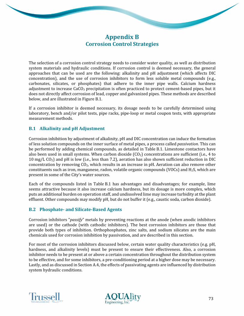
73

Appendix B Corrosion Control Strategies

The selection of a corrosion control strategy needs to consider water quality, as well as distribution system materials and hydraulic conditions. If corrosion control is deemed necessary, the general approaches that can be used are the following: alkalinity and pH adjustment (which affects DIC concentration), and the use of corrosion inhibitors to form less soluble metal compounds (e.g., carbonates, silicates, or phosphates) that adhere to the inner pipe walls. Calcium hardness adjustment to increase CaCO3 precipitation is often practiced to protect cement-based pipes, but it does not directly affect corrosion of lead, copper and galvanized pipes. These methods are described below, and are illustrated in Figure B.1.

If a corrosion inhibitor is deemed necessary, its dosage needs to be carefully determined using laboratory, bench and/or pilot tests, pipe racks, pipe-loop or metal coupon tests, with appropriate measurement methods.

B.1 Alkalinity and pH Adjustment

Corrosion inhibition by adjustment of alkalinity, pH and DIC concentration can induce the formation of less solution compounds on the inner surface of metal pipes, a process called passivation. This can be performed by adding chemical compounds, as detailed in Table B.1. Limestone contactors have also been used in small systems. When carbon dioxide (CO2) concentrations are sufficient (i.e., 4 to 10 mg/L CO2) and pH is low (i.e., less than 7.2), aeration has also shown sufficient reduction in DIC concentration by removing CO2, which results in an increase in pH. Aeration can also remove other constituents such as iron, manganese, radon, volatile organic compounds (VOCs) and H2S, which are present in some of the City’s water sources.

Each of the compounds listed in Table B.1 has advantages and disadvantages; for example, lime seems attractive because it also increase calcium hardness, but its dosage is more complex, which puts an additional burden on operation staff, and undissolved lime may increase turbidity at the plant effluent. Other compounds may modify pH, but do not buffer it (e.g., caustic soda, carbon dioxide).

B.2 Phosphate- and Silicate-Based Agents

Corrosion inhibitors “passify” metals by preventing reactions at the anode (when anodic inhibitors are used) or the cathode (with cathodic inhibitors). The best corrosion inhibitors are those that provide both types of inhibition. Orthophosphates, zinc salts, and sodium silicates are the main chemicals used for corrosion inhibition by passivation, and are described in this section.

For most of the corrosion inhibitors discussed below, certain water quality characteristics (e.g. pH, hardness, and alkalinity levels) must be present to ensure their effectiveness. Also, a corrosion inhibitor needs to be present at or above a certain concentration throughout the distribution system to be effective, and for some inhibitors, a pre-conditioning period at a higher dose may be necessary. Lastly, and as discussed in Section A.4, the effects of passivating agents are influenced by distribution system hydraulic conditions.

74

Source: USEPA’s 1992 Lead and Copper Rule Guidance Manual, Volume II: Corrosion Control Treatment.

Figure B.1: Conceptual Framework for Corrosion Control Approaches

Table B.1: Chemical Processes Used to Adjust Alkalinity and pH

Chemical Effect on pH Effect on Alkalinity Effect on DIC

Baking soda (sodium bicarbonate, NaHCO3)

Moderate increase in pH

0.60 mg/L CaCO3 alkalinity per mg/L as NaHCO3

0.14 mg/L as C per mg/L as NaHCO3

Carbon dioxide (CO2) Lowers pH None 0.27 mg/L as C per mg/L as CO2

Caustic soda (sodium hydroxide, NaOH)

Raises pH 1.55 mg/L CaCO3 alkalinity per mg/L as NaOH

None

Hydrated lime (calcium hydroxide or slaked lime, Ca(OH)2)

Raises pH 1.21 mg/L CaCO3 alkalinity per mg/L as Ca(OH)2

None

Soda ash (sodium carbonate, Na2CO3), or potash (potassium carbonate, KCO3)

Moderate increase in pH

0.90 mg/L CaCO3 alkalinity per mg/L as Na2HCO3

0.11 mg/L as C per mg/L as Na2CO3

Sodium silicates (Na2SiO3) Moderate increase in pH

Moderate increase (depends on formulation)

None

Source: USEPA 2016 Optimal Corrosion Control Treatment Evaluation Technical Recommendations.

75

Orthophosphates: These compounds include phosphoric acid (H3PO4), and mono-, di- and tri-basic sodium phosphate (NaH2PO4, Na2HPO4 and Na3PO4, respectively). They are anodic inhibitors that adsorb to surfaces and form protective films. Orthophosphate reacts with divalent metals (e.g., Pb2+ and Cu2+) to form compounds that have a strong tendency to stay in solid form and not dissolve into water. Thus they are recognized as effective agents to reduce lead and copper, and have also been used to decrease iron release.

One of the main drawbacks of orthophosphates is that they are essential nutrient of microorganisms, and have been shown to increase bacterial growth in unlined cast-iron pipes and solder in certain conditions.

Polyphosphates: These compounds are commonly used in various forms, including sodium tripolyphosphate, sodium hexametaphosphate, and other sodium and potassium polyphosphates. The primary utilization of polyphosphates is to reduce tuberculation of iron and steel, and sequester iron and manganese by binding the metals into their structures so they cannot precipitate (e.g., on sinks or clothes). They can also sequester lead and copper, keeping them in the water, and thereby increasing concentrations measured at customer taps and the risk of exposure. Thus polyphosphates are dissolved in the water rather than creating a film on pipe surfaces like orthophosphates. But because polyphosphates eventually degrade into orthophosphates through hydrolysis, the regulatory agencies do not recognize them as treatment processes to eliminate iron or manganese from water sources. Also, they are not effective corrosion inhibitors.

Polyphosphates can react according to different mechanisms: they can revert to orthophosphate and form protective films that reduce lead release, but they can also increase the release of lead (both particulate and soluble) and copper via alternative reactions. Studies suggest that the later mechanism (increase lead and copper release) may predominate in most cases. Also, polyphosphates may increase iron corrosion and release at low dosages. They can also attack and soften cement linings, asbestos-cement pipes and existing scale deposits, as well as increase the solubility of lead and copper, and prevent CaCO3 formation and deposition.

Phosphate blends: Phosphate blends can offer multiple protections, e.g., corrosion protection, hardness stabilization, red-water suppression, and sequestration of iron and manganese. In moderately hard waters, they have shown to be effective for lead and copper suppression. However, the lead corrosion scales created by phosphate blends may not be as robust as the scales created by orthophosphates, and thus, may be more susceptible to hydraulic conditions and physical disturbances. In addition, the polyphosphate portion of the blend may counteract the benefit of the orthophosphate portion in forming solid lead and copper compounds if the polyphosphate has a high affinity for sequestering lead or copper. It is unclear if blended phosphates work well to control copper corrosion and studies have shown conflicting results, especially at high alkalinity. The composition and dosage of phosphate blends are specific to the water to be treated, and depend on several parameters including pH and calcium concentration. The USEPA (2016) recommends demonstration-scale studies with adequate monitoring to determine the exact compound and dose required.

The City has been using the following phosphate blends: a 70:30 blend of poly- and ortho-phosphates at the Desalter, and a 50:50 blend of poly- and ortho-phosphates at Well 9. The selection of these inhibitors in the City’s water is discussed in Section 5.

Zinc: Zinc phosphates are bimetallic phosphates that typically combine 10 to 30% zinc with ortho- or poly-phosphates. Zinc is a cathodic inhibitor that prevents the contact between oxidizing agents (such as oxygen or chlorine) and the metal by precipitating at the cathode, thereby forming a non-

76

conductive barrier. Zinc-based inhibitors are typically used to prevent leaching of calcium from cement mortar lined and asbestos-cement pipes, and protect metal pipes by forming protective films. When zinc is combined with orthophosphates, it offers both anodic inhibition (by the orthophosphates) and cathodic inhibition (by the zinc). Evidences suggest that blends of zinc and orthophosphate are better suited to decrease iron release from cast iron pipes than agents that contain orthophosphate alone. They are also considered among the most effective corrosion inhibitors for mild steel and ductile iron because they provide both cathodic and anodic protection. With regards to controlling lead and copper corrosion, the presence of zinc in an inhibitor does not improve the effect of orthophosphate, and orthophosphate alone is sufficient.

Drawbacks of zinc-based inhibitors include the following: (1) they may be problematic for wastewater treatment plants that are limited in zinc discharge; and (2) their efficiency may be limited at high pH, high alkalinity and high calcium concentrations.

Silicates: Silicate-based corrosion inhibitors are mixtures of soda ash and silicon dioxide. Although these compounds are not commonly used, they are efficient anodic inhibitors that can sequester iron and manganese if their combined concentration does not exceed 1 mg/L, and limit red-water occurrences by forming protective films. They have also been shown to successfully reduce lead and copper release in customer taps, in the first liter of sample (i.e., first draw). Their usage is limited to soft waters with low pH and high DO concentration. Their effectiveness depends on silicate level, pH and DIC concentration. Higher doses are generally required to control lead release compared to other corrosion inhibitors, i.e., greater than 20 mg/L.

B.3 Calcium Hardness Adjustment

Precipitation of a thin layer of CaCO3 has been used to protect cement-based pipes, but it does not affect corrosion of lead, copper and galvanized pipes. CaCO3 precipitation is a function of many water quality parameters, and is also influenced by hydraulic conditions, as discussed in Section A.4.

If sufficient calcium is present in the water, increasing pH, alkalinity and/or DIC may be sufficient to favor CaCO3 precipitation. Alternatively, a number of compounds can be used to increase calcium concentration, including slaked lime (i.e., calcium hydroxide, Ca(OH)2), quicklime (i.e., calcium oxide, CaO), and calcium carbonate (CaCO3).

Excessive calcium concentrations is not desirable because it may limit a water system’s ability to raise pH (which limits metal corrosion) due to potential scaling problems.

77

APPENDIX C

Additional Water Quality Data at MWD Turnouts

78

Appendix C Water Quality Data at MWD Turnouts

Figure C.1: pH Measured at MWD T-1 and MWD T-6 Turnouts

7.2

7.4

7.6

7.8

8.0

8.2

8.4

8.6

8.8

May

-11

Aug-

11

Nov

-11

Feb-

12

May

-12

Aug-

12

Nov

-12

Feb-

13

May

-13

Aug-

13

Nov

-13

Feb-

14

May

-14

Aug-

14

Nov

-14

Feb-

15

May

-15

Aug-

15

Nov

-15

Feb-

16

May

-16

pH

MWD T-1

7.2

7.4

7.6

7.8

8.0

8.2

8.4

8.6

8.8

May

-11

Aug-

11

Nov

-11

Feb-

12

May

-12

Aug-

12

Nov

-12

Feb-

13

May

-13

Aug-

13

Nov

-13

Feb-

14

May

-14

Aug-

14

Nov

-14

Feb-

15

May

-15

Aug-

15

Nov

-15

Feb-

16

May

-16

pH

MWD T-6

79

Figure C.2: pH Measured at MWD T-5 / T-7 and MWD T-8 Turnouts

7.2

7.4

7.6

7.8

8.0

8.2

8.4

8.6

8.8

May

-11

Aug-

11

Nov

-11

Feb-

12

May

-12

Aug-

12

Nov

-12

Feb-

13

May

-13

Aug-

13

Nov

-13

Feb-

14

May

-14

Aug-

14

Nov

-14

Feb-

15

May

-15

Aug-

15

Nov

-15

Feb-

16

May

-16

pHMWD T-5/T-7

7.4

7.6

7.8

8.0

8.2

8.4

8.6

May

-11

Aug-

11

Nov

-11

Feb-

12

May

-12

Aug-

12

Nov

-12

Feb-

13

May

-13

Aug-

13

Nov

-13

Feb-

14

May

-14

Aug-

14

Nov

-14

Feb-

15

May

-15

Aug-

15

Nov

-15

Feb-

16

May

-16

pH

MWD T-8

80

Figure C.3: Orthophosphate Concentrations Measured at MWD T-1 and MWD T-6 Turnouts

0.00

0.02

0.04

0.06

0.08

0.10

0.12

0.14

0.16

0.18

0.20

0.22

May

-11

Aug-

11

Nov

-11

Feb-

12

May

-12

Aug-

12

Nov

-12

Feb-

13

May

-13

Aug-

13

Nov

-13

Feb-

14

May

-14

Aug-

14

Nov

-14

Feb-

15

May

-15

Aug-

15

Nov

-15

Feb-

16

May

-16

Ort

hoph

osph

ates

(mg/

L P)

MWD T-1

0.00

0.02

0.04

0.06

0.08

0.10

0.12

0.14

0.16

0.18

0.20

0.22

May

-11

Aug-

11

Nov

-11

Feb-

12

May

-12

Aug-

12

Nov

-12

Feb-

13

May

-13

Aug-

13

Nov

-13

Feb-

14

May

-14

Aug-

14

Nov

-14

Feb-

15

May

-15

Aug-

15

Nov

-15

Feb-

16

May

-16

Ort

hoph

osph

ates

(mg/

L P)

MWD T-6

81

Figure C.4: Orthophosphate Concentrations Measured at MWD T-5 / T-7 and MWD T-8 Turnouts

0.00

0.02

0.04

0.06

0.08

0.10

0.12

0.14

0.16

0.18

0.20

0.22

May

-11

Aug-

11

Nov

-11

Feb-

12

May

-12

Aug-

12

Nov

-12

Feb-

13

May

-13

Aug-

13

Nov

-13

Feb-

14

May

-14

Aug-

14

Nov

-14

Feb-

15

May

-15

Aug-

15

Nov

-15

Feb-

16

May

-16

Ort

hoph

osph

ates

(mg/

L P)

MWD T-5 / T-7

0.00

0.02

0.04

0.06

0.08

0.10

0.12

0.14

0.16

0.18

0.20

0.22

May

-11

Aug-

11

Nov

-11

Feb-

12

May

-12

Aug-

12

Nov

-12

Feb-

13

May

-13

Aug-

13

Nov

-13

Feb-

14

May

-14

Aug-

14

Nov

-14

Feb-

15

May

-15

Aug-

15

Nov

-15

Feb-

16

May

-16

Ort

hoph

osph

ates

(mg/

L P)

MWD T-8

Corrosion Control Study – Desktop Study Revised Draft Report

Documents

Transcript of Corrosion Control Study – Desktop Study Revised Draft Report