Correlation Risk and Optimal Portfolio Choice ANNUAL... · Correlation Risk and Optimal Portfolio...

Correlation Risk

and Optimal Portfolio Choice

ANDREA BURASCHI, PAOLO PORCHIA, and FABIO TROJANI∗

ABSTRACT

In this paper we solve an intertemporal portfolio problem with correlation risk, using a new approach

for simultaneously modeling stochastic correlation and volatility. The solutions of the model are in

closed form and include an optimal portfolio demand for hedging correlation risk. We calibrate the

model and find that the optimal demand to hedge correlation risk is a non negligible fraction of the

myopic portfolio, which often dominates the pure volatility hedging demand. The hedging demand

for correlation risk is larger in settings with high average correlations and correlation variances.

Moreover, it is increasing in the number of assets available for investment as the dimension of

uncertainty with regard to the correlation structure becomes proportionally more important.

JEL classification: D9, E3, E4, G12

Keywords: Stochastic correlation, stochastic volatility, incomplete markets, optimal portfolio choice.

First version: March 15th, 2006

This paper investigates optimal intertemporal portfolio decisions in the presence of

correlation risk. We study an incomplete markets economy in which the investment opportunity set

is stochastic due to changes in both volatilities and correlations. In such an economy, the investor has

a separate hedging demand for correlation risk. Depending on the economic scenario, we show that

optimal portfolios can look significantly different from those obtained in a more common economic

setting, in which the investment opportunity set is affected only by time-varying expected returns

and/or volatilities.

∗Andrea Buraschi is at Tanaka Business School, Imperial College London. Paolo Porchia and Fabio Trojani are at the

University of St. Gallen. We thank Francesco Audrino, Mikhail Chernov, Bernard Dumas, Christian Gouriéroux, Denis

Gromb, Robert Kosowski, Abraham Lioui, Frederik Lundtofte, Antonio Mele, Erwan Morellec, Riccardo Rebonato,

Michael Rockinger, Pascal St. Amour, Claudio Tebaldi, Nizar Touzi, Raman Uppal and seminar participants at the

EFA 2006, the Gerzensee Summer Asset-Pricing Symposium, CREST, HEC Lausanne, Inquire Europe Conference,

the NCCR FINRISK research day and the annual SFI meeting for valuable suggestions. Anna Cieslak and Dominik

Colangelo provided excellent research assistance. Paolo Porchia and Fabio Trojani gratefully acknowledge the financial

support of the Swiss National Science Foundation (NCCR FINRISK and grants 101312-103781/1 and 100012-105745/1).

The usual disclaimer applies.

The practical importance of modeling correlation risk is becoming increasingly evident. To

illustrate the portfolio impact of correlation risk, consider the case of a hedge fund with $1Bl of

assets trading in the late 1990s. Assume that the fund uses an unconstrained mean-variance portfolio

strategy constructed using historical data (one year rolling windows with data sampled at daily

frequency). Between April 1996 and early August 1998, the correlation coefficient between the 10-

year US Treasury bond yield and the Aaa corporate bond yield ranged between 0.95 and 0.99. On

August 17, 1998, Russia defaulted on its sovereign debt. Credit and liquidity spreads increased in all

markets and the correlation between US Treasury and Aaa corporate bond yields rapidly declined

reaching 0.80 in May 1999 (see Figure 1).

Insert Figure 1 about here.

In early August 1998, the average yields (standard deviation) of the two asset classes were 6.56%

(0.65) and 7.24% (0.49) respectively. Based on historical observations and assuming a 5.2% risk free

rate, the tangency portfolio would have been long $3.44Bl in corporate bonds and short $2.44Bl in

Treasury bonds. The expected portfolio return and standard deviation would have been 10.118%

and 0.455, respectively. In May 1999, however, the new tangency portfolio would have been long

$1.6Bl in corporate bonds and short $0.6Bl in Treasury bonds. The expected portfolio return has

changed from 24.2% to 12.2%. The change in the correlation coefficient alone would have induced

a large portfolio reallocation and the hedge fund would have had to liquidate $1.84Bl of corporate

bonds.1 The reallocation effect would have been even larger if the hedge fund had operated subject

to a Value-at-Risk (VaR) target, since the optimal leverage would have been even lower after the

decrease in correlation. Clearly, such large portfolio reallocations are not ex-ante optimal. If the

fund manager had anticipated that the correlation coefficient between the two asset classes was not

constant but stochastic, the optimal portfolio would have included a position to hedge unexpected

changes in correlations. This paper investigates this issue.

A vast literature has explored the implications of stochastic volatility for portfolio choice. Little

is known, however, about the impact of stochastic correlations. In part, this is because a sensible

specification of a stochastic correlation process implies tight non-linear restrictions and boundary

conditions on the asset return process: Correlations need to be bounded between −1 and +1 andthe implied covariance matrix needs to be symmetric and positive definite. Therefore, a model with

stochastic correlations can easily imply an analytically intractable covariance matrix process. In this

paper, we follow a new approach to modeling correlation risk and directly specify the covariance

matrix process as a matrix-valued affine diffusion. In this way, the model becomes tractable and

the solutions of the intertemporal optimal portfolio problem are easy to interpret economically. The

transition probabilities of the diffusion process follow a Wishart distribution and have been studied

in Bru (1991) and Gouriéroux, Jasiak, and Sufana (2004). Wishart distributions have also been

used in the statistics literature to model Bayesian priors on second moments. The optimal portfolio

1The reader may find this example evocative of the LTCM debacle. See P. Jorion (1999) for a more detailed

discussion.

1

implications, however, are not known. Since the correlation process is stochastic, we consider an

incomplete markets economy in which a constant relative risk aversion agent maximizes utility of

terminal wealth. This setting allows us to investigate the effect of the investment horizon on the

optimal holdings in risky assets. We solve the model in closed-form and characterize the hedging

demand against correlation risk in the optimal portfolio. We then use the model solutions to address

a number of questions:

(a) What is the economic importance of correlation risk in optimal portfolio choice? We calibrate

the model to historical data on international equity and US bond returns and find that, even for a

small number of assets, the hedging demand for correlation risk is larger than the hedging demand

for pure volatility risk: Correlation risk has an important impact on optimal portfolio weights. This

impact increases when the number of assets grows, since the dimension of uncertainty with regard

to the correlation structure becomes proportionally more important.

(b) How sensitive is the correlation hedging demand to the average level and variance of correlations?

We find that the correlation hedging demand is larger for high average correlations and for high

correlation variances. The economic intuition for the first effect is as follows. If correlations between

assets are high and constant, the optimal portfolio will tend to build uneven positions in the assets.

It is under these conditions that unexpected changes in the correlation coefficients have the highest

potential impact on reducing ex-post utilities. Therefore, the desire to hedge these shocks is higher

and the correlation hedging demand tends to be larger. Moreover, the higher is the conditional

volatility of the correlation, the larger is the average impact on the utility of the optimal portfolio.

Therefore, the correlation hedging demand is larger.

(c) How do both the optimal investment in risky assets and the correlation hedging demand vary

with respect to the investment horizon? This question plays an imporant role in optimal life-cycle

decisions as well as for pension fund managers. We find that the absolute correlation hedging demand

increases with the investment horizon. If the correlation hedging demand is positive (negative), this

feature implies an optimal investment in risky assets that increases (decreases) in the investment

horizon.

(d) What is the link between the persistence of correlation shocks and the demand for correlation

hedging? The persistence of correlation shocks varies across markets. In highly liquid markets like

the Treasury and foreign exchange markets, which are less affected by private information issues,

correlation shocks are less persistent. In other markets, frictions — such as asymmetric information

and differences in beliefs about future cash-flows — make price deviations from equilibrium more

difficult to be arbitraged away. Examples include both developed and emerging equity markets.

Consistent with this intuition, we find that the optimal hedging demand against correlation risk

increases with the extent of correlation shocks persistence. For example, it is higher for equity

portfolios than for portfolios formed out of long-term Treasury bonds and high credit quality US

corporate bonds.

Time-varying correlation can become an important source of risk with wide ranging economic

implications. Moskowitz (2003), for instance, argues that some pricing anomalies such as momentum

2

and size effect can be explained by stochastic correlations. Driessen, Maenhout, and Vilkov (2006)

document that the implied volatility smile is flatter for individual stock options than for index options

and attribute the difference to a priced correlation risk factor. The interest in modeling stochastic

correlation has also been spurred by financial innovation. Collateralized Debt Obligations (CDOs)

consist of pools of Credit Default Swaps (CDSs) where tranching can create flexible default risk

profiles. Since most of these new products involve a portfolio of firms, the time-variation of the

correlations is a primary source of pricing and risk management issues. The number of financial

instruments whose value depends directly on the correlation process is so large that they form a

separate asset class: "correlation derivatives". In this class we find, for example, contracts designed

to generate exposure to a foreign financial index (either a foreign interest rate or a stock market

index) but with a payoff denominated in the domestic currency. Thus, the pricing, hedging, and risk

management of these instruments explicitly depend on the correlation between the foreign index and

the exchange rate. Other correlation derivatives include foreign-exchange quanto futures and options

such as the Nikkei derivatives traded on the CME. Additional examples are differential swaps, basket

options, and rainbow options (e.g. maximum options, minimum options, spread options).

This paper draws upon a large literature on optimal portfolio choice under a stochastic investment

opportunity set. One set of papers studies optimal portfolio and consumption problems with a single

risky asset and a riskless deposit account.2 Kim and Omberg (1996) solve the portfolio problem of an

investor optimizing utility of terminal wealth, where the risk-less rate is constant and the risky asset

has a mean reverting Sharpe ratio and constant volatility. Wachter (2002) extends this setting to

allow for intermediate consumption and derives closed-form solutions in a complete markets setting.

Chacko and Viceira (2005) relax both the assumption on the preferences and the volatility. They

consider an infinite horizon economy with Epstein-Zin preferences, in which the risky asset volatility

follows a mean reverting square-root process. Liu, Longstaff, and Pan (2003) model events affecting

market prices and volatility, using the double-jump framework in Duffie, Pan, and Singleton (2000).

They show that the optimal policy is similar to that of an investor facing short-selling and borrowing

constraints, even if none is imposed. Although their approach allows for a rather general model with

stochastic volatility, they focus on a single risky asset economy. We contribute to this literature by

investigating an economy with multivariate risk factors, in which the correlation between factors is

stochastic and acts as an independent source of risk. Moreover, we investigate the optimal portfolio

implications when markets are incomplete. This aspect is especially important when volatilities and

correlations are stochastic, as it limits the ability of the portfolio manager to span the state-space

using portfolios of marketed assets. In order to derive closed-form solutions, however, we work

with CRRA preferences. This assumption is more restrictive than Chacko and Viceira (2005), who

consider a more general set of Epstein-Zin preferences.

Portfolio selection problems with multiple risky assets have been considered in a further series

of papers. The majority of these, however, assumes that volatilities and correlations are constant.

2Since the available instruments for investment consist of two assets, the resulting portfolio optimization problem

is effectively univariate, because the budget constraint allows to eliminate one portfolio weight in the optimization

problem.

3

Examples include Brennan and Xia (2002), who study optimal asset allocations under inflation risk,

and Sangvinatsos and Wachter (2005), who investigate the portfolio problem of a long-run investor

with both nominal bonds and stocks. A notable exception to the constant volatility assumption is

Liu (2007), who shows that the portfolio problem can be characterized by a sequence of differential

equations in a model with quadratic returns3 and under additional assumptions. To solve in closed-

form a concrete model with a risk-less asset, one risky bond and a stock, he assumes independence

between the state variable driving pure term structure risk and the additional risk factor influencing

the volatility of the stock return. In that model correlations are stochastic, but are restricted to being

functions of stock and bond returns volatilities. Therefore, optimal hedging portfolios do not allow

volatility and correlation risk to have separate roles. Our setting avoids deterministic dependencies

between volatilities and correlations. Moreover, it can be used to analyze portfolio choice problems

of, essentially, arbitrary dimension.

We model the stochastic covariance matrix of returns using a single-regime mean-reverting diffu-

sion process, in which the strength of the mean reversion can generate different degrees of persistence

in volatilities, correlations and co-volatilities. To obtain closed-form portfolio solutions, we refrain

from introducing also an unpredictable jump component in the joint process for returns and corre-

lations. This approach allows us to study the properties of the optimal hedging demand under a

persistent correlation process.4 A completely different approach to modeling co-movement in port-

folio choice relies on either a Markov switching-regime in correlations or on the introduction of a

sequence of unpredictable joint Poisson shocks in asset returns. Ang and Bekaert (2002) consider a

dynamic portfolio model with two i.i.d. switching regimes, one of which is characterized by higher

correlations and volatilities. Using numerical methods, they find that when the international portfo-

lio manager has access to a risk-free asset, the optimal portfolio is significatly sensitive to asymmetric

correlations between the two regimes. Our model is different from theirs because we model an in-

complete markets economy in which a single regime features persistent volatility and correlation

shocks. Moreover, the analytical solutions of the optimal portfolio allow us to study the contri-

bution of the different hedging demands for volatility and correlation risk to the overall portfolio.

Since the solutions hold for an arbitrary number of assets, we can also easily study the behavior of

correlation hedging as the number of risky assets increases. In this case, the extent of uncertainty

with regard to the correlation structure becomes proportionally more important. Das and Uppal

(2004) study systemic risk, modeled as an unpredictable common Poisson shock, in a setting with a

constant opportunity set and in the context of international equity diversification. They show that

systemic risk reduces the gain from diversification and penalizes the investor from holding levered

positions. The structure of systemic risk in their model makes changes in the correlation between

assets unpredictable and transitory. In our model, correlation and volatility shocks are persistent.

3 I.e., the interest rate, the maximal squared Sharpe ratio, the hedging coefficient vector, and the unspanned covari-

ance matrix are all quadratic fuctions of a state variables process with quadratic drift and diffusion coefficients.4Persistence of second moments has also proven to be an important dimension to “read’ traditional asset pricing

puzzles through: See, among others, Barsky and De Long (1990, 1993), Bansal and Yaron (2004) and Parker and

Julliard (2005).

4

Thus, they generate a motive for intertemporal hedging. These features yield substantially different

portfolio choice implications.

This article provides theoretical results that may prove useful to interpret the empirical evidence

emerging from the literature on hedge fund performance. Increasing evidence shows that, after

controlling for market risk, hedge fund alphas are significantly positive and persistent.5 For instance,

Kosowski, Naik, and Teo (2006) document that the average alpha of 771 long/short hedge funds is

0.51 on a monthly basis, with funds in the top decile showing alphas larger than 1.41. They test and

find that the performance is persistent and not due to luck. Clearly, part of this performance can be

attributed to managerial ability. However, our results suggest that part of these excess returns may

also compensate for the exposure to correlation risk, which is intrinsic to a long/short strategy.

This article also relates to the multivariate GARCH—literature.6 Pioneering models in this field,

as for instance Bollerslev (1987) and Bollerslev, Engle, and Wooldridge (1988), either restrict the

correlation to be constant or do not necessarily imply a positive definite covariance matrix.7 Further

important contributions include Harvey, Ruiz, and Shephard (1994), who specify a model with corre-

lation dynamics that are driven by the same factors affecting the volatility, and Barndorff-Nielsen and

Shephard (2004). An important feature of our model is precisely that correlations can have dynam-

ics not fully correlated with the factors affecting the volatility processes. Many recent multivariate

GARCH-models ensure a positive definite covariance matrix that can be estimated by a computa-

tionally feasible estimation procedure. Engle (2002) proposes a Dynamic Conditional Correlation

(DCC) specification with time-varying correlations and positive definite covariance matrices, which

builds upon the estimation of a set of univariate GARCH processes. The DCC-model and those that

extend it to include, for instance, volatility and correlation asymmetries, are analytically intractable

for dynamic portfolio choice purposes. As in multivariate GARCH-settings, our model incorporates

a persistence in volatilities and correlations. However, our model preserves the tractability required

to study the resulting optimal portfolio strategies analytically.

The article proceeds as follows: Section I summarizes the empirical properties of the correlation

between different assets and the potential implications for portfolio choice. Section II describes

the model, the main properties of the implied correlation process, and the solution to the portfolio

problem. In Section III, we calibrate the model to historical data and quantify the portfolio impact

of correlation risk. Section IV discusses some extensions of the model, which include stochastic

interest rates and a time-varying predictability of expected returns, in the spirit of Barberis (2000)

and Wachter (2002). Section V concludes. All proofs are in the Appendix.

5Papers documenting hedge fund performance include Brown, Goetzmann, and Ibbotson (1999), Fung and Hsieh

(2001), Mitchell and Pulvino (2001), Agarwal and Naik (2004), Getmansky, Lo, and Makarov (2004), Busse and Irvine

(2005), Kosowksi, Naik, and Teo (2006).6See, for instance, Poon and Granger (2003) for a review.7A well known additional issue of these specifications is the "curse of dimensionality". For n assets, one needs to

model n(n+1)2

elements of the covariance matrix, which implies that the matrices A and B have 14n2(n+ 1)2 elements.

5

I. The Time Variation of Correlations

The correlation structure of world markets varies over time. Using data ranging from 1850 to 2005 on

84 international equity markets, Goetzmann, Li, and Ronwenhorst (2005) find average correlations

ranging over time from -0.07 to 0.47. Over 1870-1913, correlations were very high. This period

is called the "golden age of capitalism" (see Rajan and Zingales, 2001) and was characterized by

high average per capita equity market capitalizations and relatively integrated financial markets.

"Following this peak" - Goetzmann, Li, and Rouwenhorst (2005) argue - "the only constant is

change". The average pairwise correlation among the four major markets (France, Germany, U.S,

and U.K.) became −0.073 (1915-1918), 0.228 (1919-1939), 0.046 (1940-1945), 0.110 (1946-1971), and0.475 (1972-2000).8 Not surprisingly, the largest negative correlation has been between the U.S.

and Germany during World War II. De Santis, Litterman, Vesval, and Winkelman (2003) confirm

these results using daily data and conclude that "both volatilities and correlations vary over time.

In addition, volatilities and correlations react with different speed to market news and may follow

different trends."9

An important strand of the literature has explored in more detail the characteristics of this

time-variation. Longin and Solnik (1995) reject the null hypothesis of constant international stock

market correlations and find that they increase in periods of high volatility. Ledoit, Santa-Clara, and

Wolf (2003) find that the level of correlation depends on the phase of the business cycle. Moreover,

Erb, Harvey, and Viskanta (1994) find that international markets tend to be more correlated when

countries are simultaneously in a recessionary state. Moskowitz (2003) documents that covariances

across portfolio returns are highly correlated with NBER recessions and that average correlations

are highly time-varying. Ang and Chen (2002) show that the correlation between US stocks and the

aggregate US market is much higher during extreme downside movements than during upside move-

ments. Longin and Solnik (2001) and Barndorff-Nielsen and Shephard (2004) find similar results.

Another important strand of the literature has provided direct evidence that market integration and

financial liberalization change the correlation of emerging markets’ stock returns with a global stock

market index (Bekaert and Harvey, 1995, 2000). The implication is that economic policies changing

the degree of market integration have structural effects on the comovement of financial markets.

To appreciate the time variation in the correlations of some asset returns, Figure 2 plots the

estimated conditional correlations based on Engle’s (2002) Dynamic Conditional Correlations (DCC)

8They use the Browne and Shapiro (1986) and Neudeck and Wesselman (1990) asymptotic distribution to run two

separate tests for the properties of international equity correlations. First, they run an element-by-element χ2 test of

the equality on the vectorized correlation matrix. Second, they test whether the average correlation is constant. They

strongly reject both null hypotheses.9To explain differences in international equity correlations, Roll (1992) suggests a Ricardian model based on country

industrial specialization. Heston and Rouwenhorst (1994) find, however, that explanations based on fiscal, monetary,

legal, cultural, and language differences dominate explanations based on industry effects. A different interpretation is

investigated by Ribeiro and Veronesi (2002), who propose a model where excess stock comovements during bad times

are obtained endogenously as a reflection of higher uncertainty.

6

model for US and German equity index daily returns (top panel), as well as for 10 year Treasury and

Aaa-corporate bond index daily returns (bottom panel), in the periods 1988—2005 and 1996—2005

respectively.


In both cases, the estimated parameters in the DCC correlation dynamics are significant at

standard significance levels, highlighting some persistence in correlations. In the top panel of Figure

2, the unconditional correlation between US and German index returns is about 0.37. The extent of

time variation, however, is large: Estimated correlations range between 0.1 in the late eighties and

more than 0.6 towards the end of the sample. Although correlations tend to spike in times of extreme

market distress, they are generally quite persistent. In the bottom panel of Figure 2, the average

correlation of Treasury bills and Aaa-bond returns is about 0.88. Before 1998, bond correlations

were very stable and even higher, most of the time, than their unconditional mean. After the 1998

Russian crisis, correlations virtually collapsed to a lowest value of less than 0.4 and became highly

time-varying, to recover to a level close to their unconditional value only towards the end of 2003.

Bond correlations also tend to be persistent, with occasional spikes during extreme market distress,

as in the most recent international financial crises, but the persistence is lower than the one observed

for stocks in our example. Since the results on the persistence of the correlation process might

be influenced by the two stage nature of the DCC, we check their robustness by using the rolling

windows estimator with correction for serial correlation suggested by De Santis et al. (2003). The

results are similar.10

The higher persistence of correlation shocks between stocks is economically plausible: The higher

liquidity of the Treasury bond market and the higher uncertainty of stocks future cash flows is likely

to make cross-sectional arbitrage trades between Treasury and corporate bonds more effective, at

least outside phases of severe credit crises. Thus, shocks to price differentials in the equity market

tend to be more persistent. For this reason, in our model a distinct set of parameters directly

controls for the persistence of correlation and volatility shocks. An additional by-product of our

specification is to allow for correlation shocks that are not perfectly spanned by shocks in volatilities.

This is consistent with the empirical evidence discussed in the literature and highlighted by our two

examples above. The potentially large persistence of the correlation processes of some asset classes,

along with the imperfect co-dependence of volatilities and correlations, suggest that the implications

of correlation risk for portfolio choice can be more important than those of stochastic volatility, which

some authors have argued to be small (see Chacko and Viceira, 2005).

10De Santis et al. (2003) find that the average half-life of the correlation process for the 18 international equity

markets with the largest stock market capitalization is about 17 months. Moreover, our DCC setting does not account

for potential long-memory patterns in the volatility and correlation processes, which many authors have successfully

modeled in several applications, typically using long time series of financial data; see, e.g., Poon and Granger (2003)

and Andersen et al. (2005) for a review. It is likely that the impact of correlation risk for optimal portofolio choice

under a long-memory dependence will be larger than the one under a short memory.

7

II. The Model

An investor with Constant Relative Risk Aversion utility over terminal wealth trades three assets,

a riskless asset with instantaneous riskless return r, and two risky assets, in a continuous-time fric-

tionless economy on a finite time horizon [0, T ]. Our analysis extends to opportunity sets consisting

of any number of risky assets and correlation factors, without affecting the existence of closed-form

solutions and their general structure. We focus on the two-dimensional setting, in order to preserve

the key economic intuition about optimal portfolio choice with stochastic correlations from notational

complications.

A. The Portfolio Allocation Problem

The investment opportunity set can be stochastic both because of changes in expected returns and

changes in conditional variances and covariances. It is well-known that in order to obtain tractable

solutions, one needs to impose restrictions on either the functional form of the squared Sharpe-ratio,

or the maximal squared Sharpe-ratio in incomplete markets. For instance, in standard settings affine

maximal squared Sharpe-ratios imply affine solutions. Given an affine state variable process, two

options are available. The first is to assume a constant risk premium and an affine inverse covariance

matrix process (see also Chacko and Viceira, 2005); the second is to assume time varying expected

returns with an affine covariance matrix process and a constant price of risk (see also Liu, 2001). In

this article, we study the portfolio impact of correlation risk in both settings. First, we solve a model

in which the maximal squared Sharpe ratio is affine in an affine covariance matrix process. In this

setting, we can more easily interpret the model parameters because the relevant state variable is the

covariance matrix of returns itself. Second, in Section IV we study the implications of correlation

risk in a model with constant risk premia and an affine inverse covariance matrix process. In the

first model, squared Sharpe ratios are increasing functions of volatilities, but can be increasing or

decreasing in correlation, depending on the sign of the prices of risk. In the second model, squared

Sharpe ratios are always decreasing in volatilities and correlation if all assets pay a positive risk

premium.

The cum dividend evolution of the price vector S = (S1, S2)0 of the risky opportunities is de-

scribed by the bivariate stochastic differential equation:

dS(t) = IS

h(r12 + Λ(Σ, t))dt+Σ

1/2(t) dW (t)i

; IS = Diag[S1, S2], (1)

where r ∈ R+, 12 = (1, 1)0,W is a standard two-dimensional Brownian motion and Σ1/2 is the positive

square root of the conditional covariance matrix Σ of returns. The available investment opportunity

set is stochastic, because of the time varying market price of risk Σ−1/2(t)Λ(Σ, t), which is a function

of the stochastic covariance matrix Σ. The constant interest rate assumption is generalized in the

model extensions discussed at the end of the paper. The diffusion process for Σ is detailed below.

Let π(t) = (π1(t), π2(t))0 denote the proportion of wealth X(t) invested in the first and the second

risky asset. An agent’s wealth evolves as:

dX(t) = X(t)£r + π(t)0Λ(Σ, t)

¤dt+X(t)π(t)0Σ1/2(t)dW (t). (2)

8

The agent selects the portfolio process π in order to maximize CRRA utility of terminal wealth with

RRA coefficient 1 − γ. If X0 = X(0) denotes the initial wealth, and Σ0 = Σ(0) denotes the initial

covariance matrix, the investor’s optimization problem is:

J(X0,Σ0) = supπE∙X(T )γ − 1

γ

¸, (3)

subject to the dynamic budget constraint (2). This setting allows us to investigate how the optimal

portfolio allocation problem varies over the life-cycle of the agent.

To model stochastic covariance matrices in a convenient way, we make use of the continuous-time

process introduced by Bru (1991) and studied by Gouriéroux and Sufana (2004) and Gouriéroux,

Jasiak, and Sufana (2004). This diffusion process is a matrix-valued extension of the univariate

square-root process that gained popularity in the term structure and the stochastic volatility liter-

ature; see, e.g., Cox, Ingersoll, and Ross (1985) and Heston (1993). Let Z be a bivariate standard

Brownian motion independent of W and define B(t) = [W (t) Z(t)] as a 2×2 matrix-valued standardBrownian motion. The diffusion process for Σ is defined as:

dΣ(t) =£ΩΩ0 +MΣ(t) + Σ(t)M 0¤ dt+Σ1/2(t)dB(t)Q+Q0dB(t)0Σ1/2(t), (4)

where Ω, M , Q being 2× 2 square matrices (with Ω invertible).

This process satisfies five important properties that make it ideal to model stochastic correlation.

First, it implies that if ΩΩ0 ≥ QQ0 then Σ is a well defined covariance matrix process. Under this

condition, the implied correlation process is well behaved and bounded between −1 and +1. Second,if ΩΩ0 = kQQ0 for some k > 1 then Σ(t) follows a Wishart distribution; see Bru (1991). This

distribution has been studied in Bayesian statistics to model priors on multivariate second moments,

but it has never been used to study optimal portfolio choice. Third, the process (4) is affine in

the sense of Duffie and Kan (1996) and Duffie, Filipovic, and Schachermayer (2003). This feature

implies closed-form expressions for all conditional Laplace transforms. Fourth, if d lnSt is a vector

of returns with Wishart covariance matrix Σ(t), then the variance of the return of a portfolio π is a

Wishart process. This is generally not the case for settings in which volatilities and correlations are

modelled by a multivariate GARCH process because GARCH models are not invariant under linear

aggregation. Fifth, process (4) is flexible enough to fit many of the empirical features of financial

asset returns, such as leverage and co-leverage, which are found to be important empirical properties

in the literature.

The only thing left to specify is the risk premium Λ(Σ, t) as a function of the state variables.

To motivate a choice for the form of Λ(Σ, t), we notice that under a power utility function, in

a Breeden’s (1979) consumption-based model, the price of risk of an asset with returns dS/S is

equal to (1 − γ)Covt [dC/C, dS/S], where dC/C is the growth rate of aggregate consumption. If

aggregate consumption follows dC/C = μCdt + a0Σ1/2dBb, where μC is the drift of consumption

growth and a and b are 2 × 1 vectors, then the risk premium of the i−th asset in our economy isgiven by (1 − γ)Covt

£dC/C, dSi/Si

¤= (1 − γ)

£a0Σ1/2dB(t)b, e0iΣ

1/2dB(t)e1¤, where ei is the i−th

unit vector. Using the property that Covt[dBa, dBb] = a0bIdt, where I is the 2× 2 identity matrix,

9

it is easy to show that the risk premium is affine in Σ(t). This result is more general and holds in

any economy whose stochastic discount factor has a diffusion term equal to a0Σ1/2dB(t)b. Thus, we

consider economies in which the vector of market prices of risk is linear in Σ(t), that is Λ(Σ, t) = Σλ

where λ = (λ1, λ2)0 ∈ R2. The same assumption is made in Heston (1993) and Liu (2001) in the caseof a scalar economy.

The first challenge in solving the investment problem (3) subject to the covariance matrix dy-

namics (4) is that markets are incomplete because of the stochastic covariance matrix. This feature is

due to the fact that the two-dimensional Brownian motion Z, appearing in the second column of the

matrix of Brownian shocks in the covariance dynamics (4), is independent of the Browniam motion

W in the returns dynamics (1). It follows that a multiplicity of equivalent martingale measures exists

in our model. To solve the portfolio problem, we consider the dual value function characterization

implied by the minimax martingale measure. He and Pearson (1991) prove that this value function

can be characterized in terms of the following static problem:11

J(X0,Σ0) = infνsupπE∙X(T )γ − 1

γ

¸, (5)

s.t. E [ξν(T )X(T )] ≤ x, (6)

where ν indexes the set of all equivalent martingale measures in the model and ξν is in the set of

associated state price densities.

In a constant covariance setting with complete markets, the market prices of risk associated with

the Brownian innovations W are simply equal to Θ = Σ1/2λ. When markets are incomplete, He and

Pearson (1991) show that each admissible market price of risk can be written as the sum of two

orthogonal components, one of which is spanned by the asset returns. Since in our setting there are

no frictions, the first component is simply given by (λ0Σ1/2,00)0 — with 0 a two-dimensional vector of

zeros — which prices the shocks to asset returns. The second component is the vector (00, ν0Σ1/2)0,

where ν is the two-dimensional vector pricing the shocks that are independent of the asset returns.

Let Θν be the matrix-valued extension of Θ that prices the matrix of Brownian motions B = [W,Z]:

Θν = Σ1/2 [λ , ν] = Σ1/2(λe01 + νe02). Given Θν , the associated martingale measure ξν(T ) takes the

form:

ξν(T ) = exp

µ−Z T

0

µr(s) +

1

2tr(Θ0ν(s)Θν(s))

¶ds−

Z T

0tr(Θν(s)

0dB(s))

¶,

where tr(·) is the trace operator. In addition, it is well-known that the optimality condition forthe optimization over π in problem (5) is X(T ) = (ψξν(T ))

1/(γ−1), where ψ is the multiplier of the

constraint (6). Therefore, problem (5) can be written as:

J(X0,Σ0) = infνE

"(ψξν(T ))

γ/(γ−1)

γ

#− 1

γ= Xγ

0 infν

1

γEhξν(T )

γ/(γ−1)i1−γ

− 1γ,

and we can focus without loss of generality on the solution of the problem:

bJ(0,Σ0) = infνEhξν(T )

γ/(γ−1)i. (7)

11See also Pliska (1986) and Cox and Huang (1989) for the Markovian complete markets case.

10

To solve this problem, we solve a corresponding Hamilton-Jacobi-Bellman equation after a change

of measure from the physical probability P to a new probability P γ . P γ is defined by the following

Radon-Nykodim derivative with respect to P :

dP γ

dP= exp

µ− γ

γ − 1

Z T

0tr(Θ0ν(s)dB(s)) +

γ2

2(γ − 1)2Z T

0tr(Θ0ν(s)Θν(s))ds

¶.

This is the Radon-Nykodim derivative that allows us to remove the stochastic integral in the expo-

nential inside the expectation of optimization problem (7):

bJ(0,Σ0) = infνEγ∙e− γγ−1

T0 r(s)ds+ γ

2(γ−1)2T0 tr(Θ0ν(s)Θν(s))ds

¸, (8)

where Eγ[·] denotes expectations under the probability P γ . Note that the expression tr(Θ0ν(s)Θν(s))

inside the expectation in equation (8) is affine in Σ(s).

Results in Schroder and Skiadas (2003) imply that if the original optimization problem has a

solution, the value function of the static problem coincides with the value function of the original

problem. The above equality holds for all times, and not just at time 0. Cvitanic and Karatzas

(1992) have shown that the solution to the original problem exists under additional restrictions on

the utility function, most importantly that the relative risk aversion does not exceed one. Cuoco

(1997) proves a more general existence result, imposing minimal restrictions on the utility function.

B. Properties of the Variance-Covariance Process

To appreciate the properties of the covariance process implied by the dynamics of (4), we study in

this section the implied correlations’ dynamics and the resulting co-dependence features of returns’

volatilities and correlations.

B.1. The correlation process

To study the correlation process under a Wishart diffusion (4), we can use Itô’s Lemma to compute

the correlation dynamics.

Proposition 1 Let ρ be the correlation diffusion process implied by the covariance matrix dynamics(4). The instantaneous drift and conditional variance of dρ(t) are given by:

Et[dρ(t)] =£A(t)ρ(t)2 +B(t)ρ(t) + C(t)

¤dt, (9)

Et[dρ(t)2] =£(1− ρ2(t)) (E(t) +G(t)ρ(t))

¤dt, (10)

where coefficients A, B, C, E, G depend exclusively on Σ11, Σ22 and the model parameters Ω, M

and Q.12

12The explicit expression for the correlation dynamics is derived in Appendix A.

11

Even if the covariance matrix process is affine, the correlation dynamics are not affine since the

correlation is a nonlinear function of variances and covariances. By construction, the instantaneous

returns correlation ρ = Σ12/√Σ11Σ22 is bounded in the interval [−1, 1]: No explicit additional

constraint on the correlation process is needed in order to ensure a well-defined return covariance

matrix process. The instantaneous drift and volatility of the correlation process are quadratic and

cubic in ρ, respectively. The correlation dynamics are not autonomous: Both the drift and the

instantaneous variance have coefficients that depend on the level of the volatilities of the first and

second asset return.

The correlation drift and the correlation volatility implied by the covariance matrix process

(4) are illustrated in Figure 3, where we make use of parameters calibrated to the estimated DCC

dynamics plotted in Figure 2.13

Insert Figure 3 about here

The calibrated correlation volatility functions are zero at the boundaries, when ρ = 1,−1, andpeak in both examples at a correlation level close to zero. The calibrated correlation drifts are

nonlinear functions of ρ, which are positive for a broad set of correlation values. Both for stocks and

bonds the correlation drift crosses the zero line approximately at the level of the sample unconditional

correlation. For correlation values below (above) this level the drift is positive (negative) and induces

a mean reversion.14 The positive unconditional correlations imply an asymmetry in the speed of

mean reversion over the support of ρ(t), which is more pronounced in the example with Treasury

and corporate bonds. We can study more precisely the mean reversion properties of our (non-linear)

correlation process by computing its pull function - see Conley, Hansen, Luttmer, and Scheinkman

(1997). The pull function ℘(x) of a nonlinear diffusion process X is the conditional probability that

Xt reaches the value x+ before x− , if initialized at X0 = x. To first order in , this probability

is given by:

℘(x) =1

2+

μX(x)

2σ2X(x)+ o( ), (11)

where μX and σX are the drift and the volatility function of X. It follows that the ratio μX(x)2σ2X(x)

is a conditional measure of the speed of mean reversion for nonlinear diffusion processes. We can

get more insight into the mean reversion properties of the correlation by studying this ratio for the

correlation process implied by the calibrated covariance matrix dynamics. The pull functions of the

calibrated correlation processes, shifted by the factor 1/2 in equation (11), are given in Panels 5 and

6 of Figure 3. They are highly asymmetric around the unconditional mean of the correlation. For

bonds, the pull function is very large, in absolute value, when the correlation is slightly above the

unconditional mean. Over a broad range of low correlation values, the pull function is much lower in

absolute value. Therefore, correlation shocks are on average more persistent below the unconditional

13Details on the calibration are provided in Section III.14As expected, this implies that for perfect positive and negative correlations the drift is negative and positive,

respectively.

12

mean of the correlation. When we calibrate the model to international equity indices, the average

level of the pull function is smaller. This feature reflects the larger persistence of correlation shocks

in this markets. The asymmetric shape of the pull function is similar to the bond markets case.

The properties of the correlation process have obvious implications for the shape of the uncondi-

tional distribution of the correlation. The stronger the asymmetry of the mean reversion, the larger

the asymmetry of the unconditional distribution of the correlation process. Figure 4 presents the

unconditional density function of the correlation, which is implied by the parameters calibrated to

the DCC dynamics of Figure 2.


As expected, the density of the calibration to Treasury and corporate bonds returns is highly

skewed and peaked towards high correlation values. The density of the calibration to equity returns

is less asymmetric and has a higher dispersion. This pattern is consistent with the weaker and less

asymmetric mean reversion of the correlation in this case.

B.2. Volatility and Correlation Leverage Effects

Due to the linear form of the drift in the dynamics (4), the model generates a linear mean reversion

in variances and covariances. The strength of this mean reversion is driven by the matrix M , which

is assumed negative semi-definite to ensure the typical mean reverting behavior and stationarity.

The matrix Q, instead, controls the co-volatility and the leverage effects between returns, volatilities

and correlations. Black’s volatility ‘leverage’ effect, that is the negative correlation between returns

and volatility, has often been found to be an empirical feature of stock returns, and it is explicitly

modeled by Heston (1993) to reproduce the empirical regularities of option-implied volatility skews.15

Roll’s (1988) correlation ‘leverage’ effect, that is the negative covariance between returns and average

correlation shocks across stocks, is also a feature supported by empirical evidence; see, e.g., Ang and

Chen (2002). The mechanism producing the volatility and the correlation leverage effects in our

model is standard and is based on the fact that the return dynamics (1) can be instantaneously

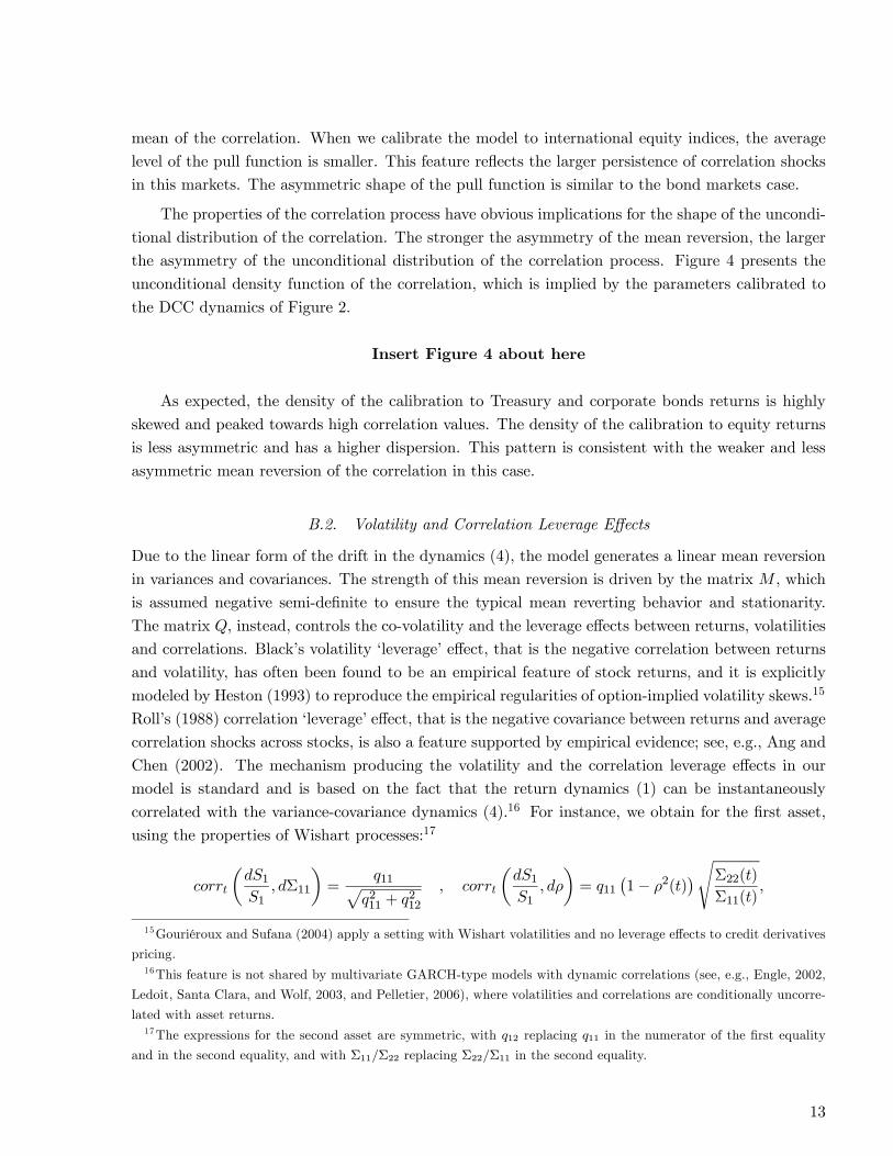
correlated with the variance-covariance dynamics (4).16 For instance, we obtain for the first asset,

using the properties of Wishart processes:17

corrt

µdS1S1

, dΣ11

¶=

q11pq211 + q212

, corrt

µdS1S1

, dρ

¶= q11

¡1− ρ2(t)

¢sΣ22(t)Σ11(t)

,

15Gouriéroux and Sufana (2004) apply a setting with Wishart volatilities and no leverage effects to credit derivatives

pricing.16This feature is not shared by multivariate GARCH-type models with dynamic correlations (see, e.g., Engle, 2002,

Ledoit, Santa Clara, and Wolf, 2003, and Pelletier, 2006), where volatilities and correlations are conditionally uncorre-

lated with asset returns.17The expressions for the second asset are symmetric, with q12 replacing q11 in the numerator of the first equality

and in the second equality, and with Σ11/Σ22 replacing Σ22/Σ11 in the second equality.

13

where q11 and q12 are the components of the first row of the matrix Q. It follows that the parameters

in the first row of this matrix control the sign of the co-dependence between returns, volatilities and

correlation shocks. When q11 and q12 are negative, the model implies a volatility-leverage and a

correlation-leverage effect.

Figure 5 presents scatter plots of simulated returns in our model, plotted against contempora-

neous changes in volatilities and correlations, for the same calibrated parameters of Figure 3.


In the calibration based on US and German stock indexes, both a correlation and a volatility

leverage effect emerge, which are highlighted by the negative relationship between returns and cor-

relations (Panels 1 and 3) and between returns and volatilities (Panels 5 and 7). These features are

due to the negative calibrated parameters q11 and q12 in Table II of Section III for this case. In

the calibration based on Treasury and corporate bonds, however, returns on the Treasury bonds are

characterized by a correlation and a volatility leverage effect (Panels 2 and 6, respectively), but the

returns of corporate bonds highlight an opposite pattern (Panels 4 and 8, respectively). This feature

is due to the mixed sign of the calibrated parameters q11 and q12 in Table II for this case.18

C. The Solution of the Investment Problem

To characterize the portfolio choice implications of process (4), we need to solve a corresponding

Hamilton-Jacobi-Bellman equation. Therefore, it is convenient to introduce the infinitesimal genera-

tor A of the process Σ. Since the joint process (Σ11,Σ22,Σ12) can be written as a trivariate diffusionprocess, A is defined in the standard way, as in Merton (1969), for functions φ = φ(Σ). Using the

particular structure of the dynamics (4) one can additionally show that A can be written in a very

compact and simple matrix form. Precisely, let φ = φ(Σ) be a smooth function. Then, the generator

A associated with the diffusion process (4) takes the form:

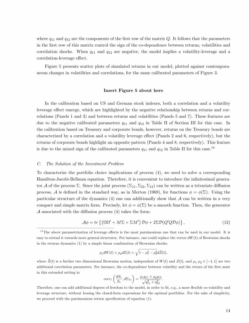
Aφ = tr©¡ΩΩ0 +MΣ+ΣM 0¢Dφ+ 2ΣD(Q0QDφ)ª , (12)

18The above parametrization of leverage effects is the most parsimonious one that can be used in our model. It is

easy to extend it towards more general structures. For instance, one could replace the vector dW (t) of Brownian shocks

in the returns dynamics (1) by a simple linear combination of Brownian shocks:

ρ1dW (t) + ρ2dZ(t) + 1− ρ21 − ρ22dZ(t),

where Z(t) is a further two dimensional Brownian motion, independent of W (t) and Z(t), and ρ1, ρ2 ∈ [−1, 1] are twoadditional correlation parameters. For instance, the co-dependence between volatility and the return of the first asset

in this extended setting is:

corrtdS1S1

, dΣ11 =ρ1q11 + ρ2q12

q211 + q212.

Therefore, one can add additional degrees of freedom to the model, in order to fit, e.g., a more flexible co-volatility and

leverage structure, without loosing the closed-form expressions for the optimal portfolios. For the sake of simplicity,

we proceed with the parsimonious return specification of equation (1).

14

where D is a matrix of differential operators.19 In this form, it is clear that this operator is affine inΣ, since the argument of the trace is affine in Σ; see also Bru (1991) and Da Fonseca, Grasselli, and

Tebaldi (2005).

We characterize the value function of the static problem (5)—(6) by solving problem (8). To

obtain the result, we take advantage of the fact that the process (4) can be shown to follow an affine

Wishart process also under the minimax martingale measure, which characterizes the solution of the

static incomplete-markets problem. The Bellman equation for problem (8) reads:

0 =∂ bJ∂t+ inf

ν

½Aν bJ + bJ ∙− γ

γ − 1r +γ

2(γ − 1)2 tr(Θ0νΘν)

¸¾,

subject to the terminal condition bJ(T,Σ) = 1. In this equation, the infinitesimal generator Aν of

the covariance matrix dynamics under the equivalent martingale measure indexed by ν is:

Aνφ = Aφ− γ

γ − 1tr©(Q0(e1λ

0 + e2ν0)Σ+Σ(λe01 + νe02)Q)Dφ

ª,

where ei is the i−th unit vector in R2; see the proofs in the Appendix. The affine structure ofthis generator is preserved and implies that the solution of problem (8) is exponentially affine in Σ,

with coefficients obtained as solutions of a system of matrix Riccati differential equations.20 These

equations can be solved in closed form.

Proposition 2 Given the covariance matrix dynamics (4), the value function of problem (3) takes

the form:

J(X0,Σ0) =Xγ0bJ(0,Σ0)1−γ − 1

γ,

where the function bJ(t,Σ) is given by:bJ(t,Σ) = exp (B(t, T ) + tr (A(t, T )Σ)) , (13)

with B(t, T ) and the symmetric matrix-valued function A(t, T ) solving the system of matrix Riccati

differential equations:

0 =dB

dt+ tr[AΩΩ0]− γ

γ − 1 r, (14)

0 =dA

dt+ Γ0A+AΓ+ 2AΛA+ C, (15)

under the terminal conditions B(T, T ) = 0 and A(T, T ) = 0, where:

Γ =M − γ

γ − 1Q0Ã

λ1 λ2

0 0

!, Λ = Q0

Ã1 0

0 1− γ

!Q , C =

γ

2(γ − 1)2

Ãλ21 λ1λ2

λ2λ1 λ22

!.

The closed-form solution of the system of matrix Riccati differential equations (14)-(15) is detailed

in Appendix A.

19The matrix differential operator D is defined by D := ∂∂Σij 1≤i,j≤2

.

20See, e.g., Reid (1972) for a review of Riccati differential equations.

15

Remark. In the literature on affine term structure models, it is well known that modeling correlated

stochastic factors is not straightforward. Duffie and Kan (1996) show that parametric restrictions

on the drift matrix of the factor dynamics have to be satisfied for a well-defined affine process to

exist. In particular, its out of diagonal elements must have the same sign. This feature restricts the

correlation structures that these models can fit (see, e.g, Duffee, 2002). In the Dai and Singleton

(2000) classification for affine Am(n) models, specific restrictions need to be imposed for the model to

be solvable: the Gaussian factors are allowed to be correlated, but the correlation between Gaussian

and square-root factors must be zero. This issue is well-recognized also in the portfolio choice

literature.21 An interesting by-product of the results of Proposition 2 is that it provides a simple

solution for the portfolio problem (3), without imposing additional restrictions on the dependence

structure between the risk factors. ¤

One advantage of the exponentially affine form of function bJ in Proposition 2 is that it allowsfor a simple description of the partial derivatives of the marginal indirect utilities of wealth with

respect to the variance and covariance factors. This property provides us with a simple and easily

interpretable solution to the incomplete-markets multivariate portfolio choice problem.

Proposition 3 Let π be the optimal portfolio obtained under the assumptions of Proposition 2. Itthen follows,

π =λ

1− γ+ 2

Ãq11A11 + q12A12

q12A22 + q11A12

!, (16)

where Aij denotes the ij−th component of the matrix A, which characterizes the function bJ(t,Σ)in Proposition 2, and the coefficients qij are the entries of the matrix Q appearing in the Wishart

dynamics (4).

The portfolio policy π is the sum of a myopic demand and a hedging demand. The hedging

demands for variance and covariance risk are simple linear functions of the elements of the matrix

A. The hedging demands on the first and second assets are, respectively, 2(q11A11 + q12A12) and

2(q11A12 + q12A22). The interpretation is simple and can be linked to the Merton (1969) solution.

The matrix A describes how the component bJ(t,Σ) of the indirect utility is affected by the statevariables driving the dynamics of Σ. Each element Aij can be rewritten as Aij =

1RRA ·

εΣijΣij, where

εΣij is the elasticity of the marginal indirect utility ∂J/∂X with respect to Σij , and RRA is the

relative risk aversion coefficient.22 Hedging demands stem from both a volatility hedging and a

covariance hedging motive. Terms proportional to A11 and A22 are pure volatility hedging demands

deriving from the own volatility risk of assets one and two, respectively. Terms proportional to

21Liu (2007) addresses this issue by assuming a triangular factor structure in an affine portfolio problem with two

risky assets.22Precisely, we have:

Aij = −1

X ∂2J∂X2

∂J∂X

· ∂J

∂Σij∂X

∂J

∂X=

1

1− γ· ∂J

∂Σij∂X

∂J

∂X,

using the envelope condition.

16

A12 are covariance hedging demands: They are due both to changes in volatility (when correlations

are different from zero) and to changes in correlations. The second set of parameters that drive

the optimal policy consists of q11 and q12, which determine the sign of the co-movement of returns,

variances, and covariances.

Despite the simple structure of the hedging policies (16), a rich set of possible hedging demands

can arise. For instance, if q11 and q12 are both negative, then volatility and correlation leverage effects

will arise for all assets. If, in addition, A11, A22 and A12 are negative, then all hedging demands for

variance and covariance risk will be positive, and the exposure to all risky assets will be increased by

the desire to intertemporally hedge variance and covariance risk. This is the situation that arises for

investors with relative risk aversion 1 − γ > 1 when we calibrate our model to international equity

returns. However, if the sign of the marginal utility sensitivities, or the sign of the co-movement

between returns, variances, and covariances, is mixed, then it is possible to obtain some hedging

demand components that are positive and some others that are negative. This is the situation that

arises when we calibrate the model to Treasury and corporate bond returns. In this setting, the

optimal correlation hedging demand for Treasury bills of an investor with risk aversion 1− γ > 1 is

positive, but that for corporate bonds is negative.

In Proposition 2, the value function is written as a function of current wealth X and the co-

variance matrix Σ. This structure enables us to easily isolate the hedging demand for variance and

covariance risk, but not the demand for correlation risk. The problem is that the hedging demand for

covariance risk is caused by both volatility and correlation risk. Therefore, we can split this demand

into two further hedging components. A volatility hedging demand against changes in returns co-

variance due to changes in assets’ volatilities, and a correlation hedging demand. This decomposition

enables us to quantify the contribution of correlation hedging to the overall hedging demand. Using

Proposition 2, it is straightforward to compute these demands, given the fact that Σ12 = ρ√Σ11Σ22.

Proposition 4 Let π be the optimal portfolio obtained under the assumptions of Proposition 2. Thehedging demand for asset i is the sum of three components πvoli , πvol/covi , πρi , which hedge, respectively,

pure volatility risk, covariance risk due to volatilities and correlation risk. The explicit expressions

for these hedging demands are as follows.

1. Pure Volatility hedging:

πvol1 = 2q11A11, πvol2 = 2q12A22. (17)

2. Covariance hedging due to volatility:

πvol/cov1 = 2q11A12ρ

rΣ22Σ11

, πvol/cov2 = 2q12A12ρ

rΣ11Σ22

. (18)

3. Correlation hedging:

πρ1 = 2A12

Ãq12 − q11ρ

rΣ22Σ11

!, πρ2 = 2A12

Ãq11 − q12ρ

rΣ11Σ22

!. (19)

17

The pure volatility hedging demands for assets one and two in equation (17) are proportional

to A11 and A22, respectively. Their signs also depend on the correlation between volatility shocks

and returns, via the coefficients q11 and q12. When A11 and A22 are negative, positive (negative)

hedging demands against volatility risk arise if and only if returns and volatility shocks are nega-

tively (positively) correlated. In equation (18), covariance hedging demands due to volatility are

proportional to the correlation level and to the sensitivity A12 of the marginal utility of wealth to

changes in covariances. This is intuitive. Higher correlations imply a higher impact of a change in

volatility on covariances, as well as a larger risk of an adverse covariance movement. Depending on

the portfolio setting, the sign of A12 can be either positive or negative. In settings of low average

correlations, in which portfolio diversification is the main objective, an increase in the correlation

between assets implies an increase in the maximal squared Sharpe ratio of the optimally invested

portfolio: Current correlations and the future risk-return tradeoff are positively related. Investors

with risk aversion 1− γ > 1, which are characterized by a utility function bounded from above, tend

to select portfolios that avoid large losses at the end of the investment horizon. If volatilities and

correlations covary negatively (positively) with returns, these investors will have a positive (nega-

tive) covariance hedging demand due to volatility, because current losses in the portfolio strategy

are hedged (exacerbated) intertemporally by the better (worse) future risk-return tradeoff.23 This

situation arises when we calibrate the model to international equity returns. However, for settings

of large positive correlations, in which optimal portfolios can even imply spread positions between

assets, the opposite might happen. In these cases, a higher correlation decreases the maximal square

Sharpe ratio and implies a negative relation between current correlations and the future risk-return

tradeoff. This situation occurs when we calibrate the model to Treasury and corporate bond returns.

The correlation hedging demand in equation (19) is also proportional to the sensitivity A12 of the

marginal utility of wealth to changes in covariances. This is intuitive. The larger A12, the larger the

sensitivity of the marginal utility of wealth to correlation shocks, and the stronger the correlation

hedging motive. Depending on the sign of q11 and q12, correlation hedging can be increasing or

decreasing in the correlation level and the ratio of the volatilities of the two assets. For example, πρ1is increasing in ρ and

pΣ22/Σ11 when q11 is negative. The relative importance of π

ρi and π

vol/coli for

the two assets depends on the relative size of q12, q11, ρ andpΣ11/Σ22.

III. Hedging Correlation Risk

In order to quantify correlation hedging in realistic portfolio choice settings, we calibrate our model

to the data. We analyze two portfolio choice scenarios. In the first scenario, we study an international

equity portfolio manager and consider a portfolio of US and German stock indices. We investigate

how correlation risk affects the desire to optimally diversify international equity risk. The second

scenario explores the case of a market-neutral hedge fund that uses spread trades to maximize re-

turns. The investor tries to build a near-arbitrage portfolio using two risky assets that are most of

the time almost perfectly positively correlated. In this case, the investor tries to optimally hedge

23The opposite happens for investors with risk aversion 1− γ < 1, which have a utility function bounded from below

by zero.

18

the risk of a leveraged position in one asset, using a corresponding short position in another asset.

For this setting, we consider 10 year Treasury and Aaa corporate bonds. In both cases, we obtain

the time series of the conditional covariance matrix for our calibrations by estimating Engle’s (2002)

multivariate DCC model.

Scenario I: International equity diversification. For equities, we use daily S&P100 and DAX index

data, from January 1988 to December 2005. Panel A of Table I presents the estimated unconditional

moments of returns, volatilities and correlations for equities.

Insert Table I about here.

During this period, the unconditional mean of US and German stock returns is about 13% and

11%, respectively. The higher unconditional volatility of German returns arises together with a

higher volatility of volatility. The unconditional correlation between the two stock indices is about

37% and the unconditional volatility of correlation is about 15%. These features generate an obvious

incentive for diversification.

Scenario II: Market neutral spread trading. For bonds, we use daily data of 10 years Treasury and

Aaa corporate bond return indices supplied by Lehman Brothers, from April 1996 to December

2005.24 The average return on Aaa bonds in Panel B of Table I is about 1.84%, slightly higher

than the 1.65% mean return of Treasury bills. The unconditional correlation is about 88%, which is

more than double the correlation between the S&P100 and the DAX index returns. The volatility

of bonds correlation is about 9.5%, which is approximately two-thirds the volatility of stock returns’

correlation. The unconditional volatility and the volatility of volatility of Treasury bills are slightly

higher than those of corporate bonds. These features generate an obvious incentive for exploiting

near-arbitrage opportunities between the Treasury and the corporate bond markets.

The optimal portfolio strategies in the two scenarios are substantially different. In the first

scenario, investors exploit the low average correlation to diversify risk between the US and the

German equity markets. To this end, they build two long positions in the corresponding assets.

In this case, correlation hedging tends to hedge unanticipated changes in the correlation structure,

which might reduce the benefits of international diversification. In the second scenario, investors

exploit the large average correlation and the low correlation volatility to develop a near arbitrage

strategy between the Treasury and the corporate bond markets. To this end, they take a long

position in corporate bonds, financed by a short position in Treasury bonds. Therefore, correlation

hedging tends to hedge unanticipated changes in correlations that might reduce the effectiveness of

this near-arbitrage strategy.

24The same exercise applied to a sample of monthly bond returns over a longer sample starting in January 1988

yielded similar results.

19

A. The Size of Correlation Hedging

We first calibrate the coefficient vector λ to match average risk premia, given estimates for the co-

variance matrix of returns. We then calibrate the covariance process (4) to the second moments of

volatilities and correlations. Using calibrated parameters, we can then decompose the total hedging

demand for asset i = 1, 2 into a pure volatility hedging component πvoli , a covariance hedging com-

ponent for volatility πvol/covi , and a correlation hedging demand πρi , as described in Proposition 4.

Table II presents the calibrated parametersM and Q for the covariance matrix dynamics in equation

(4) under the two portfolio scenarios.

Insert Table II about here.

The negative calibrated parameters q11, q12 in the first row of matrix Q in the international eq-

uity diversification scenario imply a volatility and a correlation leverage effect for all returns. In the

market neutral spread trading scenario, q11 is negative, but q12 is positive. Calibrated Treasury bond

returns exhibit a leverage effect in volatilities and correlations, but calibrated corporate bond returns

co-move positively with correlations and their volatility. In particular, this setting implies that when

correlations decrease the spread between corporate bonds and Treasury bill returns increases, consis-

tent with the "flight to quality effect" from corporate to Treasury bonds. The negative coefficients

in matrix M for stocks and bonds reflect the mean reversion in variances and covariances. The

weaker calibrated mean reversion for stocks is due to the higher volatility of the volatility and the

correlation. Therefore, shocks in stock correlations are on average more persistent than for bonds.

To compute the size of correlation hedging, covariance hedging due to volatility, and pure volatil-

ity hedging, we initialize Σ(t) at its unconditional value. We then compute the optimal hedging

demand components πvoli , πvol/covi , πρi , i = 1, 2, as defined in Proposition 4, when the average corre-

lation and the correlation volatility deviate from their sample value. We study the case in which the

investment horizon is five years and the relative risk aversion parameter is 1−γ = 3. Calibrated hedg-ing components are expressed as a percentage of the corresponding absolute myopic Merton portfolio.

Scenario I: International equity diversification. In this first calibration, we move the average correla-

tion over a grid in the interval [0.25, 0.5] and hold fixed the remaining moments of returns. Consistent

with the literature on univariate portfolio selection with stochastic volatility, pure volatility hedging

is a small fraction of the myopic portfolio: On average its absolute size is less than 2.5% of the

myopic portfolio, as illustrated in Panels 2 and 4 (triangle points) of Figure 6.


The overall hedging demand for US and German stocks is dominated by correlation hedging:

The hedging demand for correlation risk is about 7% of the myopic portfolio at the sample average

correlation and it increases up to 9% for average correlations around 48% (see Panels 1 and 3).

The absolute size of the correlation hedging is increasing in the average correlation. This result is

20

consistent with the intuition: When the average correlation is high, the available risky assets are

less able to span the risk due to unexpected shocks in the returns covariance matrix. Moreover,

negative shocks in the level of the conditional correlation tend to be more persistent, because of

the asymmetric form of the correlation mean reversion. The covariance hedging component due to

volatility in Panels 2 and 4 (circle points) is on average about 3% of the myopic portfolio at the sample

average correlation. It is typically larger than the volatility hedging demand: For the investment

in the US equity index it is more than double the corresponding volatility hedging demand. In the

international equity diversification scenario, the calibrated parameters imply a leverage effect for

volatilities and correlations of all assets. In addition, the marginal utility of wealth sensitivities of an

investor with risk aversion 1− γ > 1 to the variance and covariance factors are negative. Therefore,

all hedging demand components are positive and cumulate in the same direction. The cumulated

hedging demand is on average 11% of the myopic demand at the sample average correlation, and

about 15% of the myopic portfolio for average correlations of around 48%.

In Figure 7, we present the comparative statics of the hedging demands with respect to the

correlation volatility.


We consider values for the correlation volatility over a grid in the interval [0.05, 0.24], and hold

fixed the other moments. The absolute size of correlation hedging is increasing in the correlation

volatility: For correlation volatilities of about 24%, correlation hedging in US stocks can be as large as

11.5% of the myopic portfolio (see Panel 1). For correlation volatilities near zero, correlation hedging

tends to vanish. This is intuitive: A higher correlation volatility implies a higher risk that the myopic

portfolio will be ex-post sub-optimal. The pattern of the pure volatility hedging demand in Panels 2

and 4 (dotted points) is flatter than that of the hedging demand for correlation risk. Moreover, the

maximal volatility hedging component is less than 2% and 3.5% of the myopic portfolio, for US and

German stocks respectively.

Scenario II: Market neutral spread trading. To obtain comparative statics results for market

neutral spread trades, we consider values for the average correlation of bond returns over a grid

in the interval [0.75, 0.98]. Pure volatility hedging is a small fraction of the myopic portfolio: Its

absolute size in Panels 6 and 8 of Figure 6 (triangle points) is less than approximately 2% of the

myopic portfolio at the sample correlation. The hedging components against covariance risk caused

by volatility changes in the same panels (circle points) is on average 3.5% of the myopic portfolio. The

overall hedging demand in bonds is mostly due to correlation hedging, as illustrated by Panels 5 and

7 of Figure 6: correlation hedging is about 7% of Merton myopic portfolio for correlations of around

0.87 and about 8.5%, on average, for a correlation of 0.98. Correlation hedging is increasing in the

average correlation level. The basic intuition is similar to the one of the previous scenario. However,

the calibrated parameters imply a correlation and volatility leverage effect only for Treasury bonds,

together with an opposite pattern for corporate bonds. In addition, the marginal utility sensitivities

to volatility are negative for both asset classes, but the sensitivity to correlations and covariances

21

is positive. It follows that the market neutral spread trading scenario implies a positive (negative)

correlation hedging demand for Treasury Bills (corporate bonds). In a similar vein, the hedging

demand for covariance risk due to volatility is negative (positive) for Treasury bills (corporate bonds).

To explore the effect of the correlation volatility, we consider values in the interval [0.01, 0.16],

and hold the remaining moments fixed. Volatility hedging is a relatively flat function with respect

to the correlation volatility, both for Treasury Bills and corporate bonds, and is on average 2% of

the myopic portfolio (see Figure 7, Panels 6 and 8, triangle points). The hedging component for

covariance risk due to volatility is larger and is about 3.5% of the myopic demand (Panels 6 and 8,

dotted points). The absolute size of the correlation hedging demand can be as large as 9% of the

myopic portfolio, when the correlation volatility is about 16% (see Panels 5 and 7). As expected,

we also find that it is an increasing function of the correlation volatility and that it tends to vanish

at zero, when correlation risk also vanishes. The basic intuition is similar to that for the equity

scenario.

A.1. Time horizon

An important question addressed by the optimal portfolio choice literature is how the optimal alloca-

tion in risky assets varies with respect to the investment horizon. This question is key for investment

professionals working in the pension fund industry and for individuals deciding the composition

of their retirement accounts. Brennan, Schwartz, and Lagnado (1997), Barberis (2000), Kim and

Omberg (1996), and Wachter (2002) address this issue in the context of time-varying expected re-

turns. When volatilities are constant, they find that the optimal investment in risky assets increases

in the investment horizon. When volatilities are constant, Kim and Omberg (1996) show that for the

investor with utility over terminal wealth and for 1− γ > 1 the optimal allocation increases in the

investment horizon, as long as the risk premium is positive. Wachter (2002) extends this result to

the case of utility over intertemporal consumption under the assumption of no uncertainty about the

correlation structure of asset returns. Depending on the characteristics of this uncertainty, however,

it is reasonable to expect that the optimal demand for hedging correlation risk could mitigate, or

strengthen, the speculative components. Our model offers a simple theoretical framework to inves-

tigate the role of uncertainty on the nature of this relationship. In both the international equity

diversification and the market neutral spread trading scenarios, we find that for realistic parameter

calibrations the total optimal allocation to risky assets of an investor with risk aversion 1 − γ > 1

increases with the investment horizon. Figure 8 illustrates these effects.


All (absolute) hedging demand components are increasing in the investment horizon, both for

equities and for bonds. At short investment horizons of, e.g., 3 months, all hedging demands are

small (less than 1%) and similar. The correlation hedging demand increases faster than the other

hedging components. For instance, in the case of US index returns and at a ten year horizon, the

difference between volatility and correlation hedging (less than 2% and about 9%, respectively) is

22

quite striking. These results show that in some cases the results can change substantially when

correlation risk is taken into account.

A.2. Higher-Dimensional Portfolio Choice Settings

The previous examples considered portfolio settings with two risky assets. As the investment horizon

increases, we can expect two basic effects to influence the structure of correlation and volatility

hedging. First, the sensitivity of the marginal utility of wealth to the single correlation and volatility

factors will tend to be smaller, because optimal portfolios’ weights will tend, on average, to be

smaller. Second, the number of correlation factors increases quadratically with the dimension of

the investment universe, but the number of volatility factors increases linearly. Therefore, we can

expect the role of correlation hedging to be even more important in portfolio choice problems with

many risky assets. To investigate this issue quantitatively, we calibrate the model to an international

equity diversification scenario with three risky assets and add the FTSE100 index to the investment

opportunity set consisting of the S&P100 and the DAX indices. It is straightforward to modify

the proofs of Proposition 2 and 3 to cover the general n−dimensional case. With these results, wecompute the optimal portfolios for the model with three risky assets, after having calibrated a 3× 3Wishart covariance process to the time series of US, UK, and German index returns. Table III

summarizes the calibrated moments of returns in this setting (Panel A) and the calibrated hedging

components for correlation, volatility and covariance risk due to volatility (Panel B).

Insert Table III about here.

Correlation hedging for US and UK stocks is, on average, about 9.1% of the myopic portfolio,

larger than the correlation hedging demand for US stocks in the setting with two assets, which

was about 7.2%. The correlation hedging demand for German stocks is 6.95%, which is slightly

higher than that with two risky assets. This evidence further supports the important role played by

correlation hedging: The total average hedging demand is about 14% of the myopic portfolio, while

the average pure volatility hedging demand is only 2.4%.

IV. Robustness and Extensions

A. Risk Aversion and Interest Rate Level

The finding that correlation hedging is the most important hedging demand component, when vari-

ances and covariances are stochastic, does not hinge on the choice of the relative risk aversion para-

meter and the level of the interest rate in our calibrations. In Figure 9, we plot for the international

diversification scenario both the hedging portfolio weights and the hedging portfolio fractions of the

myopic demand as functions of the relative risk aversion.


23

Absolute hedging portfolio weights for stocks and bonds peak at a relative risk aversion of about

two, which is smaller than the one used in our calibrations. Hedging portfolios as percentages of the

myopic demand are monotonically increasing in the relative risk aversion. In both cases, correlation

hedging dominates the other hedging demands for all risk aversions considered. The dominating role

of correlation hedging is also confirmed by Figure 10, where we plot the single hedging components,

in the international diversification and the market neutral spread trading scenarios, for different

average interest rate levels from 1% to 5%.


B. Utility over consumption

The previous results focus on the case of an agent maximizing utility of terminal wealth. It is

interesting to discuss how these results could change in the case of an investor maximizing utility over

intertemporal consumption. When markets are complete and volatility is constant, Wachter (2002)

shows analytically that the optimal portfolio weights of a CRRA investor maximizing intertemporal

utility of consumption are equal to a weighted average of the portfolio weights solving a sequence

of individual terminal wealth problems. In this context, wealth can be interpreted as a bond that

pays consumption as its coupon. The value of wealth is equal to the sum of the "zeros" that pay the

optimal consumption at each date. For instance, if an agent is concerned not just about his retirement

account but also about the purchase of a house, the optimal portfolio is a weighted average of two

separate portfolios: a "retirement portfolio" and a "house portfolio". When markets are incomplete,

the previous analytical result in general does not hold. However, under the minimax martingale

measure, markets are completed by the addition of a set of securities that span the state-space and

receive zero portfolio weights in equilibrium (He and Pearson, 1991). Under this specific martingale

measure, the main results of the previous section still hold. Clearly, since the duration of lifetime

consumption is lower than the investment horizon of the agent maximizing utility over terminal

wealth, the absolute demand for risky assets would be proportionally lower.

C. Additional Dynamic Settings

The previous sections studied correlation risk for a portfolio choice problem in which expected excess

returns are linearly related to the covariance of returns (Cox, Ingersoll, and Ross, 1985, Heston,

1993 and Liu, 2001), interest rates are constant, and the covariance process, although stochastic,

is autonomous. We investigate the implications of these three assumptions with regards to the

properties of the optimal portfolio policies. We consider an economy in which: First, the risk

premium is constant. Second, interest rates are stochastic and are a function of the same state

variables that are driving asset prices. Third, additional risk factors, like the interest rate or an

aggregate market indicator, can affect the dynamic properties of the covariance matrix Σ(t) (i.e. its

speed of mean reversion and volatility).25 The economy that we consider implies that the square

25 In this way, local asymmetries in the covariance matrix dynamics can be introduced in the model. To model

asymmetric correlations across regimes, Ang and Bekaert (2002) use an i.i.d. switching regimes setting, in which one

24

Sharpe ratios are a decreasing function of the returns covariance matrix, and therefore it allows for a

direct comparison with Chacko and Viceira (2005), who study a similar, but univariate, economy with

constant interest rates. Under these assumptions, it is known that to obtain closed-form solutions it

is convenient to model directly the information matrix, i.e. Σ−1, as opposed to Σ.

To introduce additional risk factors, we model Σ−1 as a projection of a larger rank matrix Y .

For instance, if the new risk factor is the stochastic interest rate, then the 2× 2 matrix Σ−1 can beobtained from a 3× 3 Wishart process Y (t):

Σ−1 = SY S0,

where the 2× 3 matrix S is such that SS0 = id2×2.26 Given the larger rank of Y (t), the stochastic

risk-less rate r(t) can be defined directly from Y (t):

r(t) = r0+tr(Y (t)D), (20)

where r0 > 0 and D is a 3 × 3 matrix. Notice that the non-negativity of r(t) is ensured simply byassuming that the symmetric matrix D is positive definite.

The process Y satisfies the Wishart dynamics:

dY (t) = [ΩΩ0 +MY (t) + Y (t)M 0]dt+ Y 1/2(t)dBQ+Q0dB0Y 1/2(t), (21)

where the matrices Ω, M and Q are now of dimension 3 × 3 and where B = [W,Z1, Z2], with Z1

and Z2 being each a three-dimensional Brownian motion, independent of the first three-dimensional

Brownian motion W . It then follows that Σ = SY −1S0, and it is natural to define Σ1/2 as the 2× 3matrix SY −1/2.27 The return process is given by:

dS(t) = IS

"Ãr(t) + μe1

r(t) + μe2

!dt+Σ1/2(t)dW (t)

#, (22)

where the excess return vector μe = (μe1, μe2)0 ∈ R2 is constant and r(t) is given by equation (20).

This setting is effectively a six-factor model in which some interest rate risk factors might be

linked to the covariance matrix of stock returns, depending on the specific form of the matrix D in

equation (20). It is straightforward to verify that the square Sharpe ratio in this model is affine in Y .

Therefore, we can mimick the steps of the proof of Propositions 2, 3, and 4 and solve in closed-form

the portfolio choice problem (3) in this extended dynamic setting as well.

of the regimes is characterized by higher correlations and volatilities.26A possible choice for S is a 2× 3 selection matrix, like e.g.:

S =1 0 0

0 1 0.

In this case, SS0 = id2×2 and SY S0 is the 2× 2 upper diagonal sub-block of Y .27A proof of this statement is presented in Appendix A.

25

Proposition 5 The solution of the portfolio problem (3) for the returns dynamics (21)-(22) and

under a stochastic interest rate (20) is:

J(X0, Y0) =Xγ0bJ (0, Y0)1−γ − 1

γ,

where bJ(t, Y ) = exp (B(t, T ) + tr (A(t, T )Y )) ,

with B(t, T ) and the symmetric matrix-valued function A(t, T ) := A1(t, T ) + A2(t, T ) solving in

closed-form the following system of matrix Riccati differential equations:

−dBdt

= − γ

γ − 1r0 + tr(AΩΩ0), (23)

−dAi

dt= Γ0iAi +A0iΓi + 2A

0iΛiAi + Ci, (24)

where i = 1, 2, subject to A1(T, T ) = A2(T, T ) = 0. In these equations, the coefficients Γ1,Γ2 are

given by:

Γ1 =MS0S − γ

γ − 1Q0e1μ

e0S , Γ2 =M(id3×3 − S0S).

The coefficients Λ1,Λ2 are given by:

Λ1 =

⎛⎜⎜⎝1 0 0

0 1− γ 0

0 0 1− γ

⎞⎟⎟⎠ , Λ2 =

⎛⎜⎜⎝1− γ 0 0

0 1− γ 0

0 0 1− γ

⎞⎟⎟⎠and the coefficients C1, C2 are:

C1 =γ

2(γ − 1)2S0μeμe0S − γ

γ − 1S0SDS0S , C2 = −

γ

γ − 1(id3×3 − S0S)D(id3×3 − S0S).

Finally, the optimal policy for this portfolio problem reads:

π =1

1− γΣ−1

Ãμe1

μe2

!+ 2Σ−1S

⎛⎜⎜⎝q11A11 + q12A12 + q13A13

q11A21 + q12A22 + q13A23

q11A31 + q12A32 + q13A33

⎞⎟⎟⎠ . (25)

The optimal policy (25) consists of a myopic and an intertemporal hedging portfolio, which are

both proportional to the stochastic inverse covariance matrix. As noted by Chacko and Viceira

(2005), in the univariate setting the relative size of the hedging and myopic demands is independent

of the current level of volatility. This property also holds in the multivariate case, in the sense that

both policies are proportional to the inverse covariance matrix Σ−1. We calibrate the Wishart process

Y to the specification used to model the covariance matrix Σ for the special case D = 0 (constant

interest rate) and under the restriction of an autonomous covariance matrix dynamics. We then

compare the results with the findings in the previous sections. This setting is the exact multivariate

version of the univariate model studied in Chacko and Viceira (2005). We find again that correlation

26

hedging is the major determinant of the hedging demand: It amounts, on average, to approximately

60% of the total hedging demand for a Relative Risk Aversion parameter of three and an investment

horizon of five years. As expected, the sign of the hedging demands in this setting is different since

the squared Sharpe ratio implied by the model is decreasing in the covariance matrix. The myopic

portfolio is time varying, via the variation of the inverse covariance matrix Σ−1. This variation

is also partly reflected in the time variation of hedging demands. Figure 11 presents a summary

of the calibrated myopic portfolio weights (left panels) and hedging demands (right panels) in the

international equity diversification and the market neutral spread trading scenarios, when expected

excess returns are assumed constant.


D. Multivariate Portfolio Choice and Predictability

The previous models can be extended to study an important issue in multivariate portfolio choice,

such as the joint impact of correlation risk and predictability on the optimal hedging demand. A

large literature has studied the consequences of predictability for portfolio choice with a single risky

asset. Campbell and Viceira (1999), Kim and Omberg (1996), and Wachter (2002) propose tractable

portfolio choice settings that can be handled analytically. The first paper uses approximate solu-

tions to characterize the portfolio of an infinitely-lived investor. The second one derives closed-form

solutions for an incomplete-market setting with power utility over terminal wealth. The last one,

obtains closed-form optimal portfolios for a complete markets setting with intermediate consump-

tion. Important evidence on predictability has also been studied by Barberis (2000), who shows the

portfolio choice impact of predictability under estimation risk, and Xia (2001), who documents the

effect of learning about predictability.

Using our previous results, it is easy to model predictability in our framework. Let Y be a matrix

containing all the priced factors and let the risk premium on each asset depend on a time-varying

predicting factor and on asset returns’ volatilities, and correlations:

Λ(t, Y ) =

Ãλ1Σ11 + λ2Σ12 + Y13

λ1Σ21 + λ2Σ22 + Y23

!. (26)

Given the 3× 3 Wishart process Y in equation (21), let Σ = SY S0, where the matrix S is such that

S0S = id2×2, and define Σ1/2 = SY 1/2.28 To complete the specification, the risk premium is modeled

as Λ(t, Y ) = SY (t)λ, with λ = (λ1, λ2, 1)0 ∈ R3. The resulting returns dynamics are given by:

dS(t) = IS

h(r12 + SY (t)λ) dt+Σ1/2(t)dW (t)

i, (27)

with the risk premium satisfying (26). In this specification, expected excess returns are driven by

the variance-covariance risk factors and the additional predictability factors Y13 and Y23, which can

28 In the most simple case, for instance, S can be chosen to be a selection matrix of the form S =1 0 0

0 1 0.

27

be correlated with the covariance matrix dynamics. Clearly, if λ1 = λ2 = 0 the predictability factors

are the only variables affecting risk premia, as in Kim and Omberg (1996) and Wachter (2002), who

assume a predictability factor following an Ornstein-Uhlenbeck process and a constant volatility of

returns. In all other cases, returns variances and covariances will also affect risk premia. It is easy

to verify that the squared Sharpe ratio in this and similar models is equal to λ0Y (t)λ. Therefore,

the same solution method used in Proposition 2 and 3 leads to closed-form solutions for the optimal

portfolio.

V. Discussion and Conclusions

In this article we have analyzed the importance of correlation risk for portfolio decisions, and have

proposed a new simple approach to embed stochastic correlation in optimal portfolio choice. The

flexibility of the model allows us to study correlation hedging in settings that can account for several

stylized features of asset returns, including volatility/correlation persistence and leverage effects. We

show that correlation hedging contributes to the overall portfolio in a qualitatively and quantita-

tively significant way. Examples of calibrated economies show that correlation hedging can be a

non-negligible fraction of Merton’s myopic portfolio, while volatility hedging is typically small. The

correlation hedging demand is larger for settings with extreme average correlations and higher corre-

lation variances, and is increasing in the number of assets available for investment, as the dimension

of uncertainty with regard to the correlation structure becomes proportionally more important.

The proposed approach to modeling time-varying correlations, as well as the analytical opti-

mal portfolio results, can prove useful in investigating a number of further economic questions. For

instance, an important strand of the empirical asset pricing literature has investigated the character-

istics of hedge funds performance.29 Kosowski, Naik, and Teo (2006) document that, after controlling

for market risk, hedge fund alphas are significantly positive and persistent. Hedge funds in the top

decile of the return distribution have alphas well in excess of 1% per month. They test and find

that the performance is persistent and not due to luck. A proposed interpretation of this evidence is

that these funds have superior managerial ability. However, about 34% of the hedge funds classify

as long/short funds and 7% as fixed income arbitrage funds. Our results suggest that part of these

excess returns may also compensate for the exposure to correlation risk, which is key in long/short

strategies. Since these alphas are typically obtained without explicitly controlling for exposure to

correlation risk, it would be a very interesting empirical question to investigate the extent of the link

between exposure to correlation risk and hedge funds alphas.

Correlation risk plays also a direct role in the pricing, hedging, and risk management of correla-

tion derivatives, such as quantos. In these financial instruments, the underlying asset is denominated

in one currency, while the instrument itself is settled in another currency at some fixed exchange

rate. Such products are attractive for portfolio managers or hedge funds who wish to have exposure

29See, for instance, Brown, Goetzmann and Ibbotson (1999), Fung and Hsieh (2001), Mitchell and Pulvino (2001),

Agarwal and Naik (2004), Getmansky, Lo, and Makarov (2004), Busse and Irvine (2005), Kosowksi, Naik, and Teo

(2006).

28

to a foreign asset, without carrying the corresponding exchange rate risk. Well-known examples

include differential swaps (also known as quantity-adjusted swaps, guaranteed exchange rate swaps,

Libor differential swaps), quanto options, quanto equity swaps, and quanto futures (such as the

Nikkei Future traded on the CME). In these cases, the pricing, hedging, and risk management of

these instruments depend directly on the correlation between the risk factors (see Reiner, 1992 and

Dravid, Richardson, and Sun, 1993). For these reasons, these instruments are also referred to by

practitioners as "correlation products". In differential swaps, for instance, the dealer commits to

paying a floating rate on a fixed US dollar notional amount, rather than on a fixed amount in the

foreign currency, as with a typical cross-currency swap. This commitment exposes the dealer to

changes in the correlation between the Libor and the exchange rates. Since static hedging strategies

are generally not feasible, the dealer must manage the residual correlation risk by using optimal

portfolio techniques to model correlation risk.

Correlation risk also plays an important role in the trading of multi-asset (rainbow) options.

A multi-asset option is a derivative security whose payoff depends on the future values of several,

possibly correlated, underlying assets. Typical examples are basket, spread, outside barrier options

and options on the minimum/maximum of several assets. Since equity correlation risk cannot be

hedged as precisely as volatility risk, the current market practice of equity derivatives desks is simply

to monitor their correlation exposure and try to avoid risk peaks in certain correlation pairs by man-

aging the product flow via dynamic price margins, and by using index options to hedge the "average"

correlation risk within the index basket. However, specific correlation risk in individual stock pairs

remains. The results of this article provide an alternative strategy for managing correlation risk.

Finally, correlation risk is a key issue in the credit derivative market as the likelihood of a

default of one credit may affect the likelihood of default of another (default correlation). Examples

of correlation-based products also include instruments written on baskets of credits, such as CDOs

and first-to-default (FTD) swaps. Investors in FTD structures sell protection on a reference portfolio

of names and assume exposure to the first default that takes place within the pre-defined basket of

credits. Upon occurrence of a default, the protection seller needs to identify the protection buyer

for the loss on the defaulted credit, calculated on the basis of the full face value of the FTD basket.

Clearly, the ex-ante value of these instruments is highly sensitive to the correlations structure in the

basket.

References

Agarwal, V., Naik, N. Y., 2004, Risk and portfolio decisions involving hedge funds, Review of Financial Studies

17, 63-98.

Andersen, T. G., Bollerslev, T., Christoffersen, P. F., and F. Diebold, 2005, Volatility Forecasting, Working Paper.

Ang, A. and G. Bekaert, 2002, International Asset Allocation with Regime Shifts, Review of Financial Studies 15,

1137-1187.

Ang, A. and J. Chen, 2002, Asymmetric Correlations of Equity Portfolios, Journal of Financial Economics 63,

443-494.

29

Bansal, R. and A. Yaron, 2004, Risks for the Long-run: A Potential Resolution of Asset Pricing Puzzles, Journal

of Finance 59, 1481-1509.

Barberis, N., 2000, Investing for the Long-Run when Returns are Predictable, Journal of Finance 55, 225-264.

Barndorff-Nielsen, O. E. and N. Shephard, 2004, Econometric Analysis of Realized Covariation: High Frequency

Covariance, Regression and Correlation in Financial Economics, Econometrica 72, 885-925.

Barsky, R. B. and J. B. De Long ,1990, Bull and Bear Markets in the Twentieth Century, Journal of Economic

History 50, 1—17.

Barsky, R. B. and J. B. DeLong, 1993, Why Does the Stock Market Fluctuate ?, Quarterly Journal of Economics

108, 291-312.

Bekaert, G. and C. R. Harvey, 1995, Time-varying World Market Integration, Journal of Finance 50, 403-444.

Bekaert, G. and C. R. Harvey, 2000, Foreign Speculators and Emerging Equity Markets, Journal of Finance 55,

565-613.

Bollerslev, T., 1987, A Conditionally Heteroskedastic Time Series Model for Speculative Prices and Rates of Return,

Review of Economics and Statistics 69, 542-547.

Bollerslev, T., Chou, R., and K. Kroner, 1992, ARCH Modelling in Finance: A Review of the Theory and Empirical

Evidence, Journal of Econometrics 52, 5-59.

Bollerslev, T., Engle, R., and J. Woolridge, 1988, A Capital Asset Pricing Model with Time-Varying Covariances,

Journal of Political Economy 96, 116-131.

Brown, S., Goetzmann, W., and R. Ibbotson, 1999, Offshore Hedge Funds: Survival and Performance, 1989-95,

Journal of Business 72, 91-117.

Bru, M. F., 1991, Wishart Processes, Journal of Theoretical and Applied Probability 4, 725-743.

Brennan, M. J. and Y. Xia, 2001, Assessing Asset Pricing Anomalies, Review of Financial Studies 14, 905-942.

Brennan, M. J., Schwartz, E.S., and R. Lagnado, 1997, Strategic Asset Allocation, Journal of Economic Dynamics

and Control 21, 1377-1403.

Browne, M.W and A. Shapiro, 1986, The Asymptotic Covariance Matrix of Sample Correlation Coefficients under

General Conditions, Linear Algebra and Its Applications 82, 169-176.

Busse, J. and P. Irvine, 2006, Bayesian Alphas and Mutual Fund Persistence, The Journal of Finance 61, 2251-2288.

Campbell, J. and L. Viceira, 1999, Consumption and Portfolio Decisions when Expected Returns Are Time Varying,

The Quarterly Journal of Economics 114, 433-495.

Chacko, G. and L. Viceira, 2005, Dynamic Consumption and Portfolio Choice with Stochastic Volatility in Incom-

plete Markets, Review of Financial Studies 18, 1369-1402.

Conley, T. G., Hansen, L. P., Luttmer, G. J., and J. A. Scheinkman, 1997, Short-Term Interest Rates as Subordi-

nated Diffusions, Review of Financial Studies 10, 3, 525-577.

Cox, J. C., Ingersoll, J. E., and S. Ross, 1985, An Intertemporal General Equilibrium Model of Asset Prices,

Econometrica 53, 2, 363-384.

Cox, J. C. and Chi-Fu Huang, 1989, Optimal Consumption and Portfolio Policies when Asset Prices Follow a

Diffusion, J. Econ. Theory 49, 33-83.

30

Cuoco, D., 1997, Optimal Consumption and Equilibrium Prices with Portfolio Constraints and Stochastic Income,

Journal of Economic Theory 72, 33—73.

Cvitanic, J. and I. Karatzas, 1992, Convex Duality in Constrained Portfolio Optimization, Annals of Applied

Probability 2, 767-818.

Da Fonseca, J., Grasselli, M., and C. Tebaldi, 2005, Wishart Multi-Dimensional Stochastic Volatility, Working

Paper, University of Verona.

Dai, Q. and K. Singleton, 2000, Specification Analysis of Affine Term Structure Models, Journal of Finance 50,

1943-1978.

Das, S. R. and R. Uppal, 2004, Systemic Risk and International Portfolio Choice, Journal of Finance 59, 2809-2834.

De Santis, G., Litterman, B., Vesval A., and K. Winkelmann, 2003, Covariance Matrix Estimation, Modern Invest-

ment Management, Bob Litterman and the Quantitative Resources Group, Goldman Sachs Asset Management,

John Wiley & Sons, New Jersey.

Dravid, A., Richardson, M., and T. S. Sun, 1993, Pricing Foreign Index Contingent Claims: An Application to

Nikkei Index Warrants, Journal of Derivatives 1, 1, 33-51.

Driessen, J., Maenhout, P., and G. Vilkov, 2006, Option-Implied Correlations and the Price of Correlation Risk,

Working paper, University of Amsterdam.

Duffee, G. R., 2002, Term Premia and Interest Rates Forecasts in Affine Models, Journal of Finance 52, 405-443.

Duffie, D., Filipovic, D., and W. Schachermayer, 2003, Affine Processes and Applications in Finance, Annals of

Applied Probability 13, 984-1053.

Duffie, D. and R. Kan, 1996, A Yield-Factor Model of Interest Rates, Mathematical Finance 4, 379-406.

Duffie D., Pan J., and K. Singleton, 2000, Transform Analysis and Asset Pricing for Affine Jump Diffusions,

Econometrica 68, 6, 1343-1376.

Engle, R., 2002, Dynamic Conditional Correlation - a Simple Class of Multivariate GARCH Models, Journal of

Business and Economic Statistics 20, 339-350.

Engle, R. F., and K. F. Kroner, 1995, Multivariate Simultaneous Generalized ARCH, Econometric Theory 11, 1,

122-50.

Erb, C., Harvey, C. and T. Viskanta, 1994, Forecasting International Equity Correlations, Financial Analysts

Journal November/December, 32-45.

Fung, W. and D. Hsieh, 2001, The Risk in Hedge Fund Strategies: Theory and Evidence from Trend Followers,

Review of Financial Studies 14, 313-341.

Getmansky, M., Lo, A., and I. Makarov, 2004, An Econometric Model of Serial Correlation and Illiquidity of Hedge

Fund Returns, Journal of Financial Economics 74, 529-610.

Goetzmann, W. N., Li, L., and K. G. Rouwenhorst, 2005, Long-Term Global Market Correlations, Journal of

Business, 78, 1-38.

Gouriéroux, C. and R. Sufana, 2004, Derivative Pricing with Multivariate Stochastic Volatility: Application to

Credit Risk, Working paper, University of Toronto.

Gouriéroux, C., Jasiak, J., and R. Sufana, 2004, The Wishart Autoregressive Process of Multivariate Stochastic

Volatility, Journal of Econometrics, forthcoming.

31

Harvey, A., Ruiz, E., and N. Shephard, 1994, Multivariate Stochastic Variance Models, Review of Economic Studies

61, 2, 247-64.

He, H. and N. D. Pearson, 1991, Consumption and Portfolio Policies with Incomplete Markets and Short Sales

Constraints: The Infinite Dimensional Case, Journal of Economic Theory 54, 259-304.

Heston, S. L., 1993, A Closed-Form Solution for Options with Stochastic Volatility with Applications to Bond and

Currency Options, Review of Financial Studies 6, 327-343.

Heston, S. L. and L. G. Rouwenhorst, 1994, Does Industrial Structure Explain the Benefits of International

Diversification? Journal of Financial Economics 36, 3-27.

Jorion, P., 1999, Risk Management Lessons from Long-Term Capital Management, Working paper.

Kim, T. S. and E. Omberg, 1996, Dynamic Nonmyopic Portfolio Behavior, Review of Financial Studies 9, 141-161.

Kosowski, R., Naik, N., and M. Teo, 2007, Does Money Grow on Hedge Funds? A Bayesian and Bootstrap Analysis,

Journal of Financial Economics, forthcoming.

Ledoit, O., Santa-Clara, P., and M. Wolf, 2003, Flexible Multivariate GARCH Modeling with an Application to

International Stock Markets, Review of Economics and Statistics 85, 735-747.

Liu, J., 2001, Dynamic Portfolio Choice and Risk Aversion, Working paper, Rady School of Management.

Liu, J., Longstaff F., and J. Pan, 2003, Dynamic Asset Allocation with Event Risk, Journal of Finance 58, 231-259.

Liu, J., 2007, Portfolio Selection in Stochastic Environments, Review of Financial Studies, 20, 1-39.

Longin, F. and B. Solnik, 1995, Is the Correlation in International Equity Returns Constant: 1960-1990? Journal

of International Money and Finance 14, 1, 3-26.

Longin, F. and B. Solnik, 2001, Extreme Correlation of International Equity Markets, Journal of Finance 56,

649-675.

Merton, R. C., 1969, Lifetime Portfolio Selection: The Continuous-Time Case, Review of Economics and Statistic

51, 247-257.

Mitchell, M. and T. Pulvino, 2001, Characteristics of Risk in Risk Arbitrage, Journal of Finance 56, 2135-2175.

Moskowitz, T., 2003, An Analysis of Covariance Risk and Pricing Anomalies, Review of Financial Studies 16,

417-457.

Munk, C. and C. Sorensen, 2004, Optimal Consumption and Investment Strategies with Stochastic Interest Rates,

Journal of Banking and Finance 28, 1987-2013.

Neudecker, H. and A. M. Wesselman, 1990, The Asymptotic Covariance of Sample Correlation Matrix, Linear

Algebra and Its Applications 127, 589-599.

Parker, J. A. and C. Julliard, 2005, Consumption Risk and the Cross-section of Expected Returns, Journal of

Political Economy, 113, 185-222.

Pelletier, D., 2006, Regime Switching for Dynamic Correlations, Journal of Econometrics 127, 445-473.

Pliska, S., 1986, A Stochastic Calculus Model of Continuous Trading: Optimal Portfolios, Mathematics of Opera-

tions Research 11, 371-382.

Poon, S. H. and C. Granger, 2003, Forecasting Volatility in Financial Markets: A Review, Journal of Economic

Literature 41, 478-539.

32

Rajan, R. and L. Zingales, 2001, The Great Reversals: The Politics of Financial Developments in the 20th Century,

NBER Working Paper No. W8178, National Bureau of Economic Research, Cambridge, MA.

Reid, W. T., 1972, Riccati Differential Equations, Academic Press, New York.

Reiner, E., 1992, Quanto Mechanics, Risk 5, 10, 59-63.

Ribeiro, R. and P. Veronesi, 2002, The Excess Comovement of International Stock Markets in Bad Times: A

Rational Expectations Equilibrium Model, Working paper, University of Chicago

Roll, R., 1988, The International Crash of October, 1987, Financial Analysts Journal September-October, 19-35.

Roll, R., 1992, Industrial Structure and the Comparative Behavior of International Stock Market Indeces, Journal

of Finance 47, 3-41.

Sangvinatsos, A. and J. Watcher, 2005, Does the Failure of the Expectations Hypothesis Matter for Long-Term

Investors? Journal of Finance 60, 179-230.

Schroder, M. and C. Skiadas, 2003, Optimal Lifetime Consumption-Portfolio Strategies under Trading Constraints

and Generalized Recursive Preferences, Stochastic Processes and Their Applications 108, 155-202.

Wachter, J., 2002, Portfolio and Consumption Decisions Under Mean-Reverting Returns: An Exact Solution for

Complete Markets, Journal of Financial and Quantitative Analysis 37, 63-91.

Xia, Y., 2001, Learning about Predictability: The Effect of Parameter Uncertainty on Dynamic Asset Allocation,

Journal of Finance 56, 205-246.

33

Appendix A: Proofs of Theorems

Proof of Proposition 1: The dynamics of the correlation process implied by the Wishart covariance matrix diffusion(4) is computed using Itô’s Lemma. Let

ρ(t) =Σ12(t)

Σ11(t)Σ22(t)(A1)

be the instantaneous correlation between the returns of the first and the second risky assets and denote by σij andqij the ij−th component of the volatility matrix Σ1/2 and the matrix Q in equation (4), respectively. Applying Itô’sLemma to (A1) and using the dynamics for Σ11, Σ22 and Σ12, implied by (4), it follows:

dρ = −ρ

2

q211 + q221Σ11

+q212 + q222

Σ22+ (ρ2 − 2)q11q12 + q21q22√

Σ11Σ22+ (1− ρ2)

m21Σ11 +m12Σ22√Σ11Σ22

dt

− ρ

Σ11Σ22(Σ22σ11q11 +Σ11σ12q12)−

σ12q11 + σ11q12√Σ11Σ22

dW1

− ρ

Σ11Σ22(Σ11σ22q12 +Σ22σ21q11)−

σ22q11 + σ21q12√Σ11Σ22

dW2

− ρ

Σ11Σ22(Σ22σ11q21 +Σ11σ12q22)−

σ11q22 + σ12q21√Σ11Σ22

dZ1

− ρ

Σ11Σ22(Σ11σ22q22 +Σ22σ21q21)−

σ21q22 + σ22q21√Σ11Σ22

dZ2 (A2)

Therefore, the instantaneous drift of the correlation process is a quadratic polynomial with state dependent coefficients:

E [dρ(t)| Ft] = A(t) ρ(t)2 +B(t) ρ(t) + C(t) dt, (A3)

where coefficients A(t), B(t) and C(t) are given by:

A(t) =q11q12 + q21q22

Σ11(t)Σ22(t)−m21

Σ11(t)

Σ22(t)−m12

Σ22(t)

Σ11(t), (A4)

B(t) = −12

q211 + q221Σ11(t)

+q212 + q222Σ22(t)

, (A5)

C(t) = −2q11q12 + q21q22

Σ11(t)Σ22(t)+m21

Σ11(t)

Σ22(t)+m12

Σ22(t)

Σ11(t). (A6)

The instantaneous conditional variance of the correlation process is easily obtained from equation (A2) using theindependence of Brownian motions Z and W , and it is a third order polynomial with state dependent coefficients:

E dρ(t)2 Ft = 1− ρ2(t)q211 + q221Σ11(t)

+q212 + q222Σ22(t)

+ 2ρ(t)q11q12 + q21q22

Σ11(t)Σ22(t)dt.

This concludes the proof.¤

34

Proof of Proposition 2: Since markets are incomplete, we follow He and Pearson (1991) and represent any marketprice of risk as the sum of two orthogonal components, one of which is spanned by the asset returns. Since in our

setting there are no frictions, the first component is Σ1/2λ0

, where λ is the vector that prices the shocks to asset

returns and 0 is a two-dimensional vector of zeros. The second component is0

Σ1/2ν, where ν is the vector pricing

the shocks that are independent of the asset returns. Let Θν be the matrix-valued extension of Θ that prices the matrixof Brownian motions B = [W,Z]:

Θν = Σ1/2 [ λ , ν ] = Σ1/2(λe01 + νe02), (A7)

where e1 = (1, 0)0 and e2 = (0, 1)0. Given Θν , the associated martingale measure implies a process ξν of stochasticdiscount factors, defined for t ∈ [0, T ] by:

ξν(t) = e−rt−tr(t0 Θ0ν(s) dB(s)+

12

t0 Θ0ν(s)Θν(s)ds). (A8)

Our dynamic portfolio choice problem admits an equivalent static representation by means of the following dual problem,as shown by He and Pearson (1991):

J(x,Σ0) = infνsupπE X(T )γ − 1

γ, (A9)

s.t. E [ξν(T )X(T )] ≤ x, (A10)

where X(0) = x. In what follows, we focus on the solution of problem (A9)-(A10). The optimality conditions for theinnermost maximization is:

X(T ) = (ψξν(T ))1

γ−1 , (A11)

where the Lagrange multiplier for the static budget constraint is

ψ = xγ−1E ξν(T )γ

γ−11−γ

.

It then follows:J(x,Σ0) = xγ inf

ν

1

γE ξν(T )

γγ−1

1−γ− 1

γ. (A12)

Using (A8) and (A12), one can notice that the solution requires the computation of the expected value of the exponentialof a stochastic integral. A simple change of measure reduces the problem to the calculation of the expectation of theexponential of a deterministic integral. Let P γ be the probability measure defined by the following Radon-Nykodimderivative with respect to the physical measure P :

dP γ

dP= e

−tr γγ−1

T0 Θ0ν(s) dB(s)+

12

γ2

(γ−1)2T0 Θ0ν(s)Θν(s)ds

. (A13)

We denote expectations under P γ by Eγ [·]. Then, the minimizer of (A12) is the solution of the following problem:30

J(0,Σ0) = infνE ξν(T )

γγ−1

= infνEγ e

− γγ−1 rT+

γ

2(γ−1)2 tr(T0 Θ0ν(s)Θν(s)ds)

= infνEγ e

− γγ−1 rT+

γ

2(γ−1)2 tr(T0 Σ(s)ds(λλ0+νν0))

. (A14)

Notice that the expression in the exponential of the expectation in (A14) is affine in Σ. By Girsanov Theorem, underthe measure P γ the stochastic process Bγ , defined as

Bγ(t) = B(t) +γ

γ − 1t

0

Θν(s)ds

is a 2 × 2 matrix of standard Brownian motions. Therefore, the process (4) is an affine process also under the newprobability measure P γ :

dΣ(t) = ΩΩ0 + M − γ

γ − 1Q0(e1λ

0 + e2ν0) Σ(t) +Σ(t) M − γ

γ − 1Q0(e1λ

0 + e2ν0)

0dt

+Σ1/2(t)dBγ(t)Q+Q0dB(t)γ 0Σ1/2(t). (A15)

30Strictly speaking, this holds for γ ∈ (0, 1). For γ < 0, minimizations are replaced by maximizations and all formulasfollow with the same type of arguments.

35

Using Feynman Kac formula, it is known that if the optimal ν and J solve the probabilistic problem (A14), then theymust also be a solution of the following Hamilton Jacobi Bellman (HJB) equation:

0 =∂J

∂t+ inf

νAJ + J − γ

γ − 1r +γ

2(γ − 1)2 tr(Σ(λλ0 + νν0) , (A16)

subject to the terminal condition J(T,Σ) = 1, where A is the infinitesimal generator of the matrix-valued diffusion(A15), which is given by:

A = tr ΩΩ0 + M − γ

γ − 1Q0(e1λ

0 + e2ν0) Σ+Σ M − γ

γ − 1Q0(e1λ

0 + e2ν0)

0D

+ tr(2ΣDQ0QD), (A17)

where

D :=∂

∂Σ11

∂∂Σ12

∂∂Σ21

∂∂Σ22

. (A18)

The generator is affine in Σ. The optimality condition for the optimal control ν, implied by HJB equation (A16), is:

1

γ − 1Σν =∂

∂νtr Q0(νe02)

0Σ+Σνe02QDJJ

=∂

∂νtr

DJJ

Q0(νe02)0Σ+Σνe02Q

DJJ

.

Applying rules for the derivative of trace operators, the right hand side can be written as Σ DJJ+ DJ0

JQ0e2. It follows

that

ν = (γ − 1) DJJ+DJ 0

JQ0e2.

We now compute the generator (A17) associated with this solution. To this end, note that

λe01 + νe02 = λe01 + (γ − 1)DJJ+DJ 0

JQ0e2e

02.

Substituting the expression for ν obtained in equation (A17), we obtain the generator

A = tr ΩΩ0 + M − γ

γ − 1Q0e1λ

0 Σ+Σ M − γ

γ − 1Q0e1λ

00D + 2ΣDQ0QD

− γ tr Q0e2e02Q

DJJ+DJ 0

JΣ+Σ

DJJ+DJ 0

JQ0e2e

02Q D

= tr ΩΩ0 + M − γ

γ − 1Q0e1λ

0 Σ+Σ M − γ

γ − 1Q0e1λ

00D + 2ΣDQ0QD

− γJ tr ΣDJJ+DJ 0

JQ0e2e

02Q

DJ+D0

J

0.

Substitution of the last expression for A into the HJB equation (A16) yields the following partial differential equationfor J :

−∂J

∂t= tr ΩΩ0 + M − γ

γ − 1Q0e1λ

0 Σ+Σ M − γ

γ − 1Q0e1λ

00D + 2ΣDQ0QD J

+γ

γ − 1J −r + tr (Σλλ0)

2(γ − 1) − γ

2J tr Σ

DJJ+DJ 0

JQ0e2e

02Q

DJJ+DJ 0

J

0

,

subject to the boundary condition J(Σ, T ) = 1. The affine structure of this problem suggests an exponentially affinefunctional form for its solution:

J(t,Σ) = exp(B(t, T ) + tr(A(t, T )Σ),

for some state independent coefficients B(t, T ) and A(t, T ). After inserting this functional form into the differentialequation for J , the guess can be easily verified. The coefficients B and A are the solutions of the following system ofRiccati equations:

−dB

dt= tr(AΩΩ0)− γ

γ − 1r,

−tr dA

dtΣ = tr Γ0AΣ+AΓΣ+ 2AQ0QAΣ− γ

2(A0 +A)Q0e2e

02Q(A

0 +A)Σ+γ

2(γ − 1)2 λλ0Σ ,

36

with terminal conditions B(T, T ) = 0 and A(T, T ) = 0, where

Γ =M − γ

γ − 1Q0e1λ

0.

For a symmetric matrix function A, the second differential equation implies the following matrix Riccati equation:

0 =dA

dt+ Γ0A+AΓ+ 2AQ0(id2×2 − γe2e

02)QA+

γ

2(γ − 1)2 λλ0. (A19)

Defining

Λ = Q0(id2×2 − γe2e02)Q = Q0 1 0

0 1− γ Q , C =γ

2(γ − 1)2 λλ0, (A20)

the system of matrix Riccati equations in the statement of Proposition 2 is obtained. These differential equations arecompletely integrable, so that closed-form expressions for J (and hence for J) can be computed.

Given a solution for A, function B is obtained by simple integration:

B(t, T ) =γ

γ − 1 r (T − t)− trT

t

A(s, T )ΩΩ0 ds .

The solution for A is:

A(t, T ) = A+ eΘ0(T−t) −A−1 + 2

T

t

eΘ(T−s)ΛeΘ0(T−s)ds

−1

eΘ(T−t), (A21)

where Θ = Γ+ 2ΛA, e· is the matrix exponential function and matrix A is the solution of the quadratic system

Γ0A+AΓ+ 2AΛA+C = 0. (A22)

To prove that (A21) is indeed the solution for A, we apply the variation of constants method. Let τ = T − t denotetime to maturity. With this variable, the Riccati differential equation for A is:

dA

dτ= Γ0A(τ) +A(τ)Γ+ 2A(τ)ΛA(τ) + C , (A23)

subject to initial condition A(0) = 0. Let A∗ be the solution of the following quadratic matrix equation

Γ0A∗ +A∗Γ+ 2A∗ΛA∗ + C = 0,

and define A(τ) := K(τ) +A∗. After inserting this guess for A into equation (A23), we see that K(τ) must solve thematrix differential equation

dK

dτ= Γ∗

0K(τ) +K(τ)Γ∗ + 2K(τ)ΛK(τ), (A24)

subject to initial condition K(0) = −A∗, where Γ∗ := Γ+ 2ΛA∗. Define

K(τ) = exp(Γ∗τ)0H(τ) exp(Γ∗τ),

for some matrix valued function H(τ). It then follows,

dK

dτ= Γ∗

0exp(Γ∗τ)0H(τ) exp(Γ∗τ) + exp(Γ∗τ)0H(τ) exp(Γ∗τ)Γ∗ + exp(Γ∗τ)0

dH(τ)

dτexp(Γ∗τ)

= Γ∗0K(τ) +K(τ)Γ∗ + exp(Γ∗τ)0

dH(τ)

dτexp(Γ∗τ).

By comparing the last expression with (A24), the function H(τ) must satisfy the following matrix differential equation:

dH

dτ= 2H(τ) exp(Γ∗τ)Λ exp(Γ∗τ)0H(τ) ,

subject to initial condition H(0) = −A∗. After integrating this equation, using the definition of K(τ) and recallingthat A(τ) = K(τ) +A∗, we obtain (A22). This concludes the proof.

¤

37

Proof of Proposition 3: In order to recover the optimal portfolio policy we have, from the proof of Proposition 2:

X∗(t) =:1

ξν∗(t)E[ξν∗(T )X

∗(T ) |Ft] = ψ1

γ−1 ξν∗(t)1

γ−1 J(t,Σ(t)). (A25)

For the Wishart dynamics (4), Itô’s lemma applied to both sides of (A25) gives, for every state Σ:

X∗(t) trπ1 π20 0 Σ1/2dB = X∗(t) tr

1

1− γΘ0ν∗dB +

DJ 0

JΣ1/2dBQ+Q0dB0Σ1/2 . (A26)

This implies

Σ1/2π1 0π2 0 =

1

1− γΘν∗ + 2Σ

1/2AQ0.

We conclude that portfolio weight π = (π1, π2)0 is

π =λ

1− γ+ 2AQ0e1 =

1

1− γλ1λ2

+ 2q11A11 + q12A12q12A22 + q11A12

. (A27)

This concludes the proof of the proposition.¤

38

Proof of Proposition 4: To obtain the optimal hedging demand in terms of the state variables Σ11, Σ22, and ρ,write Σ12 = ρ

√Σ11Σ12 and note that:

−X∂2J∂2X

∂2J

∂ρ∂X=−X∂2J∂2X

∂2J

∂Σ12∂X

∂Σ12∂ρ

= A12

√Σ11Σ22.

This is the closed form expression for the wealth-scaled ratio of marginal utilities with respect to ρ and X. Forvolatilities, the same argument gives, for i, j = 1, 2, where i 6= j:

−X∂2J∂2X

∂2J

∂Σii∂X= Aii +

−X∂2J∂2X

∂2J

∂Σ12∂X

∂Σ12∂Σii

= Aii +A12ρ

2

Σjj

Σii. (A28)

This is the closed form expression for the wealth-scaled ratio of marginal utilities with respect to Σii and X, when ρ istreated as an explicit state variable, in addition to Σ11 and Σ22. The first term on the right hand side of equation (A28)is the one that corresponds to the direct effect of Σii on the value function. The second term is the one that correspondsto the indirect effect of Σii, via the feedback of Σii on Σ12. To compute the corresponding hedging demand it is thenenough to use Merton (1969)’s results and to calculate the projection coefficients of dΣ11, dΣ22 and dρ on the spacespanned by dS1/S1 and dS2/S2, using the available dynamics. After collecting terms proportional to A12

√Σ11Σ22,

A11, A22, A12ρ2 Σ11/Σ22 and A12

ρ2 Σ22/Σ11, respectively, the desired decomposition follows. This concludes the

proof of the proposition.¤

39

Proof of Proposition 5: We first prove a useful technical result on the form of the inverse covariance matrixΣ−1 = (SY S0)−1 when SS0 = id2×2.

Lemma 1 Let SS0 = id2×2. It then follows:

(SY S0)−1 = SY −1S0.

Proof of Lemma 1: Since SY S0 is symmetric, we have:

SY S0 = QΛQ0 , (SY S0)−1 = QΛ−1Q0, (A29)

where Q is a 2× 2 matrix of eigenvectors of SY S0 and Λ a diagonal 2× 2 matrix of eigenvalues. Similarly,

Y = QΛQ0 , Y −1 = QΛ−1Q0,

where Q is a 3×3matrix of eigenvectors of Y and Λ a diagonal matrix of eigenvalues. We first show that the eigenvectorsof SY S0 are all vectors qi such that S0qi is an eigenvector of Y . Indeed, let qi = S0qi be an eigenvector of Y . It thenfollows,

SY S0qi = SY qi = λiSqi = λiqi,

where λi is an eigenvalue of both SY S and Y . In particular, the non-zero elements of Λ are a subset of the nonzeroelements of Λ. We also have, for all eigenvectors qi of SY S:

Sqi = SS0qi = qi.

Since S has rank 2, one eigenvector qi of SY S0 must be such that Sqi = 0. Without loss of generality, let this eigenvectorbe q3. We then have:

SQ = [ Q 02×1 ]

andSY −1S0 = SQΛ−1Q0S0 = [ Q 02×1 ] Λ

−1 Q0

01×2= QΛ−1Q0,

because the non zero elements in Λ are a subset of those in Λ. From (A29), we conclude:

(SY S0)−1 = SY −1S0,

as desired. This concludes the proof of the Lemma.

We now proceed with the proof of Proposition 5. Let ν = [ν1, ν2, ν3], where ν1, ν2, ν3 ∈ R3. It turns out, that thevalue function can be written in the form:

J(x, Y0) = xγ infν

1

γE ξν(T )

γγ−1

1−γ− 1

γ=

xγJ(0, Y0)1−γ − 1

γ,

subject to the constraint Sν1 = 0, where

E ξν(T )γ

γ−1 = Eγ e− γγ−1

T0 r(s)ds+ γ

2(γ−1)2 tr(T0 Σ(s)−1dsμeμe0+ T

0 Y (s)ds(ν1ν01+ν2ν

02+ν3ν

03))

= Eγ e− γγ−1 (r0+tr(

T0 Y (s)dsD))+ γ

2(γ−1)2 tr(T0 Y (s)ds(S0μeμe0S+ν1ν

01+ν2ν

02+ν3ν

03)) , (A30)

for a probability measure P γ defined by the density:

dP γ

dP= e

−tr γγ−1

T0 Θ0ν(s)dB+

12

γ2

(γ−1)2T0 Θ0ν(s)Θν(s)ds

.

The 3× 3 matrix Θν of market prices of risk is defined by:

Θν = Σ1/20Σ−1μe 03×1 03×1 + [ ν1 ν2 ν3 ] ,

where ν1, ν2, ν3 ∈ R3 and Σ1/2ν1 = 0. For convenience, we parameterize Θν as:

Θν = Y −1/2 [ S0SY S0μe 03×1 03×1 ] + Y 1/2 [ ν1 ν2 ν3 ] ,

40

where νi = Y −1/2νi for i = 1, 2, 3. In this parametrization, the constraint Σ1/2ν1 = 0 reads Sν1 = 0, and the objectivefunction (A30) follows. Similarly to the previous portfolio choice settings, the following decomposition of Θν applies:

Θν = Y −1/2S0SY S0μee01 + Y 1/2ν,

where ei it the i−th unit vector in R3. The dynamics of Y under the probability P γ are:

dY = ΩΩ0 + M − γ

1− γQ0ν0 Y − γ

1− γQ0e1μ

e0SY S0S

+Y M − γ

1− γQ0ν0

0− γ

1− γS0SY S0μee01Q dt+ Y 1/2dBγQ+Q0dB0γY 1/2.

These dynamics are affine in Y . It follows, that the infinitesimal generator of the process Y is:

A = tr ΩΩ0 + M − γ

1− γQ0ν0 Y − γ

1− γQ0e1μ

e0SY S0S D

+tr Y M − γ

1− γQ0ν0

0− γ

1− γS0SY S0μee01Q D + tr 2YDQ0QD . (A31)

The HJB equation for J can be then written as:

0 =∂J

∂t− γ

γ − 1J(r0 + tr(Y D)) + infν

AJ + γ

2(γ − 1)2 Jtr Y (S0μeμe0S + ν1ν01 + ν2ν

02 + ν3ν

03) , (A32)

subject to Sν1 = 0 and the terminal condition J(T, Y ) = 1. For i = 2, 3, the optimal control νi is given by:

νi = (γ − 1)DJJ+DJ 0

JQ0ei,

The optimal control ν1 satisfies the optimality condition

1

γ − 1Y ν1 = YDJJ+DJ 0

JQ0e1 + S0λ,

where λ ∈ R2 is the vector of Lagrange multipliers of the constraint Sν1 = 0. This gives:

ν1 = (γ − 1)DJJ+DJ 0

JQ0e1 + Y −1S0λ .

Using the constraint

0 = Sν1 = (γ − 1) SDJJ+DJ 0

JQ0e1 + SY −1S0λ ,

it follows:

λ = −(γ − 1)SY S0S DJJ+DJJ

Q0e1.

Therefore, the optimal control ν1 reads explicitly:

ν1 = (γ − 1) id3×3 − Y −1S0SY S0SDJJ+DJ 0

JQ0e1.

It then follows:ν = ν1e

01 + ν2e

02 + ν2e

03

= (γ − 1) DJJ+DJ 0

JQ0 − Y −1S0SY S0S

DJJ+DJ 0

JQ0e1e

01 .

After inserting the expression for the optimal ν in equation (A31), we obtain the generator:

A = tr ΩΩ0 +MY − γ

1− γQ0e1μ

e0SY S0S + YM 0 − γ

1− γS0SY S0μee01Q D + 2YDQ0QD

−γtr Q0QDJJ+DJ 0

JY −Q0e1e

01Q

DJJ+DJ 0

JS0SY S0S D

−γtr YDJJ+DJ 0

JQ0Q− S0SY S0S

DJJ+DJ 0

JQ0e1e

01Q D .

41

Using the properties of the trace operator, we obtain the more compact expression:

A = tr ΩΩ0 +MY − γ

1− γQ0e1μ


1− γS0SY S0μee01Q D + 2YDQ0QD

−γJtr YDJJ+DJ 0

JQ0Q− S0SY S0S

DJJ+DJ 0

JQ0e1e

01Q

DJ+D0

J.

Substitution of the last expression for A in the HJB equation (A32), using the form of the optimal control ν and theidentity SS0 = id2×2, yields the following partial differential equation for J :

−∂J

∂t= tr ΩΩ0 +MY − γ

1− γQ0e1μ


1− γS0SY S0μee01Q D + 2YDQ0QD J

−γ

2Jtr Y

DJJ+DJ 0

JQ0Q− S0SY S0S

DJJ+DJ 0

JQ0e1e

01Q

DJJ+DJ 0

J

− γ

γ − 1J(r0 + tr(Y D)) +γ

2(γ − 1)2 Jtr(Y S0μeμe0S),

subject to the terminal condition J(T, Y ) = 1. The affine structure of this problem suggests an affine functional formfor J :

J(t, Y ) = exp (B(t, T ) + tr(A(t, T )Y )),

where the functions B(t, T ) and A(t, T ) are state-independent and satisfy the boundary condition B(T, T ) = 0 andA(T, T ) = 0. It follows that B and A satisfy the following system of differential equations:

−dB

dt= − γ

γ − 1r0 + tr(AΩΩ0)

−tr dA

dtY = tr M 0A+AM − γ

γ − 1(S0SAQ0e1μ

e0S + S0μee01QAS0S) Y

+tr 2((1− γ)AQ0QA+ γS0SAQ0e1e01QAS

0S) +γ

2(γ − 1)2S0μeμe0S − γ

γ − 1D Y

with terminal condition B(T, T ) = 0 and A(T, T ) = 0. In order to solve the equation for A, it is useful to apply thefollowing decomposition:

dA

dtY =

dA

dtS0SY +

dA

dt(id3×3 − S0S)Y

=dA

dtS0S(S0SY ) +

dA

dt(id3×3 − S0S)(id3×3 − S0S)Y.

We can use this decomposition to obtain two systems of matrix Riccati differential equations for A1 := AS0S andA2 := A(id3×3 − S0S). The system of differential equations for A1 is:

−dA1

dt= S0SM 0A1 −

γ

γ − 1S0μee01QA1 +A0

1MS0S − γ

γ − 1A01Q

0e1μe0S

+2(1− γ)A01Q

0QA1 + γA01Q

0e1e01QA1 +

γ

2(γ − 1)2S0μeμe0S − γ

γ − 1S0SDS0S

= S0SM 0 − γ

γ − 1S0μee01Q A1 +A0

1 MS0S − γ

γ − 1Q0e1μ

e0S

+2A01Q

0 (1− γ)id3×3 + γe1e01 QA1 +

γ

2(γ − 1)2S0μeμe0S − γ

γ − 1S0SDS0S,

subject to the terminal condition A1(T, T ) = 0. The system of matrix Riccati differential equations for A2 is:

−dA2

dt= (id3×3 − S0S)M 0A2 +A0

2M(id3×3 − S0S) + 2(1− γ)A02Q

0QA2

− γ

γ − 1(id3×3 − S0S)D(id3×3 − S0S),

subject to the terminal condition A2(T, T ) = 0. The unique solution for A is obtained as A = A1 +A2.In order to recover the optimal portfolio policy, we follow similar arguments as in the proof of Proposition 3 and

use the relation:X∗(t) =:

1

ξν∗(t)E[ξν∗(T )X

∗(T ) |Ft] = ψ1

γ−1 ξν∗(t)1

γ−1 J(t, Y (t)). (A33)

42

Itô’s lemma applied to both sides of (A33) gives, for every state Σ:

X∗(t) trπ1 π20 0 Σ1/2dB = X∗(t) tr

1

1− γΘ0ν∗dB +

DJ 0

JY 1/2dBQ+Q0dB0Y 1/2 .

This implies (recall that Σ1/2 = SY −1/2):

Y −1/2S0π1 0π2 0 =

1

1− γΘν∗ + 2Y

1/2AQ0.

We conclude that the portfolio weight π = (π1, π2)0 is

π =1

1− γΣ−1μe + 2Σ−1SAQ0e1

=1

1− γΣ−1 μe1

μe2+ 2Σ−1S

q11A11 + q12A12 + q13A13q11A21 + q12A22 + q13A23q11A31 + q12A32 + q13A33

.

This concludes the proof of Proposition 5.¤

43

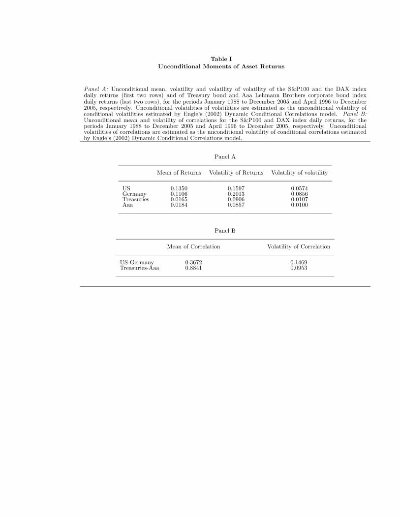
Table IUnconditional Moments of Asset Returns

Panel A: Unconditional mean, volatility and volatility of volatility of the S&P100 and the DAX indexdaily returns (first two rows) and of Treasury bond and Aaa Lehmann Brothers corporate bond indexdaily returns (last two rows), for the periods January 1988 to December 2005 and April 1996 to December2005, respectively. Unconditional volatilities of volatilities are estimated as the unconditional volatility ofconditional volatilities estimated by Engle’s (2002) Dynamic Conditional Correlations model. Panel B:Unconditional mean and volatility of correlations for the S&P100 and DAX index daily returns, for theperiods January 1988 to December 2005 and April 1996 to December 2005, respectively. Unconditionalvolatilities of correlations are estimated as the unconditional volatility of conditional correlations estimatedby Engle’s (2002) Dynamic Conditional Correlations model.

Panel A

Mean of Returns Volatility of Returns Volatility of volatility

US 0.1350 0.1597 0.0574Germany 0.1106 0.2013 0.0856Treasuries 0.0165 0.0906 0.0107Aaa 0.0184 0.0857 0.0100

Panel B

Mean of Correlation Volatility of Correlation

US-Germany 0.3672 0.1469Treasuries-Aaa 0.8841 0.0953

Table IICalibrated Parameters of the Wishart covariance matrix process

Calibrated matrices M and Q for returns dynamics (1) under Wishart covariance matrix process (4) forΩΩ0 = kQQ0 and k = 10. Parameters have been calibrated to the estimated unconditional moments ofreturns and volatilities in Table I for US/German equity index returns and Treasury bond/Aaa corporatebond index returns.

M Q

US-Germany−0.2816 0.0147

0.0502 −0.1548−0.0009 −0.00300.0028 0.0022

Treasuries-Aaa−0.4563 0.0273

0.0659 −0.3951−0.0007 0.0020

0.0024 0.0019

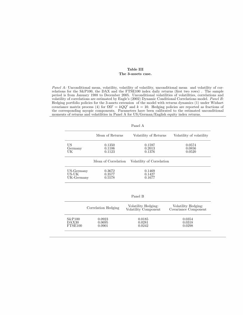
Table IIIThe 3-assets case.

Panel A: Unconditional mean, volatility, volatility of volatility, unconditional mean and volatility of cor-relations for the S&P100, the DAX and the FTSE100 index daily returns (first two rows) . The sampleperiod is from January 1988 to December 2005. Unconditional volatilities of volatilities, correlations andvolatility of correlations are estimated by Engle’s (2002) Dynamic Conditional Correlations model. Panel B:Hedging portfolio policies for the 3-assets extension of the model with returns dynamics (1) under Wishartcovariance matrix process (4) for ΩΩ0 = kQQ0 and k = 10. Hedging policies are reported as fractions ofthe corresponding myopic components. Parameters have been calibrated to the estimated unconditionalmoments of returns and volatilities in Panel A for US/German/English equity index returns.

Panel A

Mean of Returns Volatility of Returns Volatility of volatility

US 0.1350 0.1597 0.0574Germany 0.1106 0.2013 0.0856UK 0.1123 0.1376 0.0520

Mean of Correlation Volatility of Correlation

US-Germany 0.3672 0.1469US-UK 0.3577 0.1427UK-Germany 0.5578 0.1677

Panel B

Correlation Hedging Volatility Hedging:Volatility Component

Volatility Hedging:Covariance Component

S&P100 0.0923 0.0185 0.0354DAX30 0.0695 0.0281 0.0318FTSE100 0.0901 0.0242 0.0298

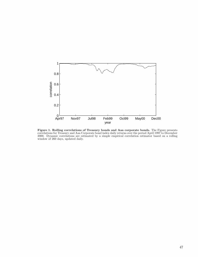
Apr97 Nov97 Jul98 Feb99 Oct99 May00 Dec000

0.2

0.4

0.6

0.8

1

year

corr

elat

ion

Figure 1. Rolling correlations of Treasury bonds and Aaa corporate bonds. The Figure presentscorrelations for Treasury and Aaa Corporate bond index daily returns over the period April 1997 to December2000. Dynamic correlations are estimated by a simple empirical correlation estimator based on a rollingwindow of 260 days, updated daily.

47

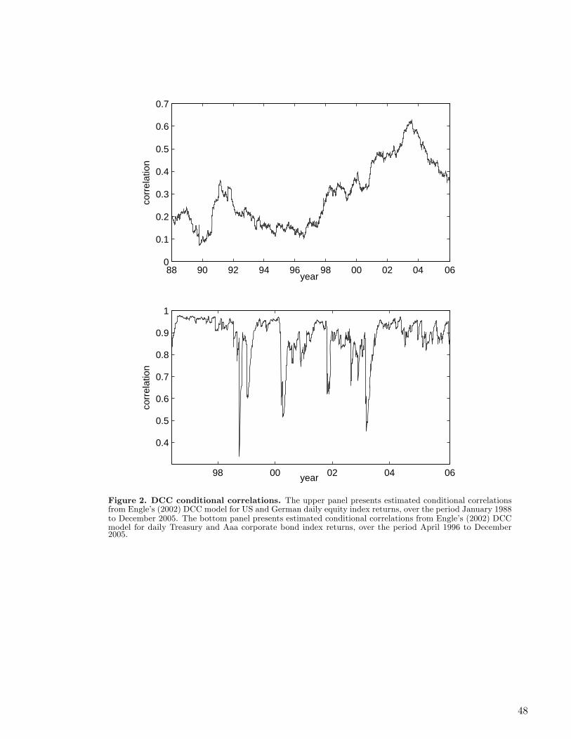
88 90 92 94 96 98 00 02 04 060

0.1

0.2

0.3

0.4

0.5

0.6

0.7

year

corr

elat

ion

98 00 02 04 06

0.4

0.5

0.6

0.7

0.8

0.9

1

corr

elat

ion

year

Figure 2. DCC conditional correlations. The upper panel presents estimated conditional correlationsfrom Engle’s (2002) DCC model for US and German daily equity index returns, over the period January 1988to December 2005. The bottom panel presents estimated conditional correlations from Engle’s (2002) DCCmodel for daily Treasury and Aaa corporate bond index returns, over the period April 1996 to December2005.

48

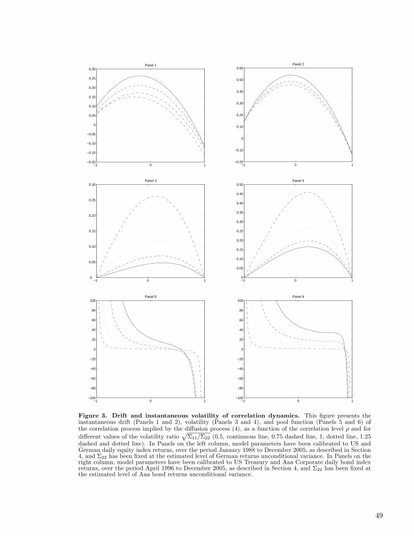
−1 0 1−0.20

−0.15

−0.10

−0.05

0

0.05

0.10

0.15

0.20

0.25

0.30Panel 1

−1 0 1−0.20

−0.10

0

0.10

0.20

0.30

0.40

0.50

0.60Panel 2

−1 0 10

0.05

0.10

0.15

0.20

0.25

0.30Panel 3

−1 0 10

0.05

0.10

0.15

0.20

0.25

0.30

0.35

0.40

0.45

0.50Panel 4

−1 0 1−100

−80

−60

−40

−20

0

20

40

60

80

100Panel 5

−1 0 1−100

−80

−60

−40

−20

0

20

40

60

80

100Panel 6

Figure 3. Drift and instantaneous volatility of correlation dynamics. This figure presents theinstantaneous drift (Panels 1 and 2), volatility (Panels 3 and 4), and pool function (Panels 5 and 6) ofthe correlation process implied by the diffusion process (4), as a function of the correlation level ρ and fordifferent values of the volatility ratio Σ11/Σ22 (0.5, continuous line, 0.75 dashed line, 1, dotted line, 1.25dashed and dotted line). In Panels on the left column, model parameters have been calibrated to US andGerman daily equity index returns, over the period January 1988 to December 2005, as described in Section4, and Σ22 has been fixed at the estimated level of German returns unconditional variance. In Panels on theright column, model parameters have been calibrated to US Treasury and Aaa Corporate daily bond indexreturns, over the period April 1996 to December 2005, as described in Section 4, and Σ22 has been fixed atthe estimated level of Aaa bond returns unconditional variance.

49

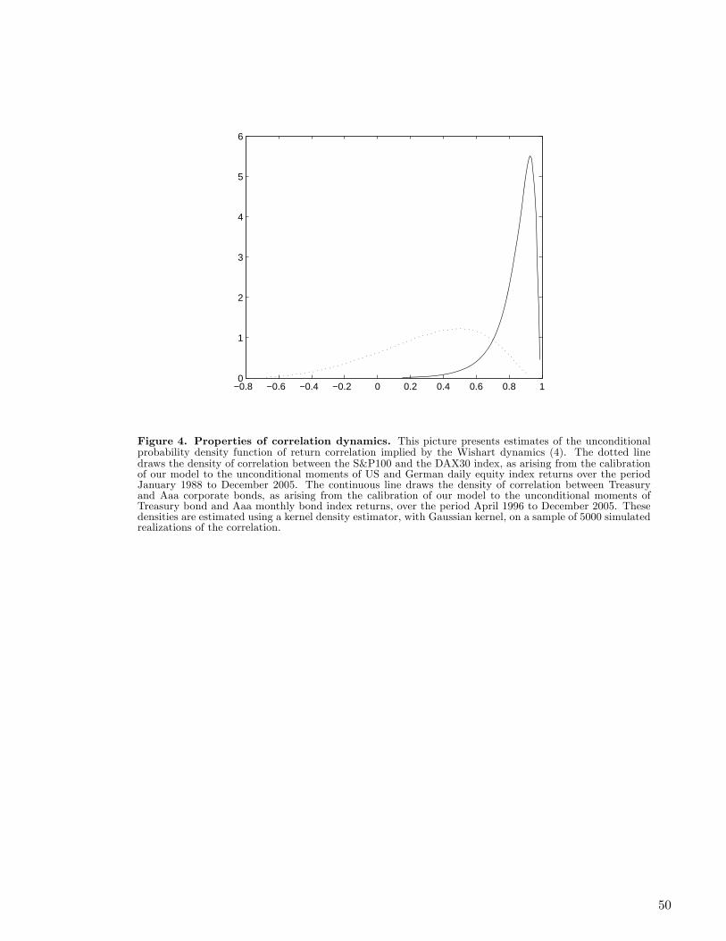
−0.8 −0.6 −0.4 −0.2 0 0.2 0.4 0.6 0.8 10

1

2

3

4

5

6

Figure 4. Properties of correlation dynamics. This picture presents estimates of the unconditionalprobability density function of return correlation implied by the Wishart dynamics (4). The dotted linedraws the density of correlation between the S&P100 and the DAX30 index, as arising from the calibrationof our model to the unconditional moments of US and German daily equity index returns over the periodJanuary 1988 to December 2005. The continuous line draws the density of correlation between Treasuryand Aaa corporate bonds, as arising from the calibration of our model to the unconditional moments ofTreasury bond and Aaa monthly bond index returns, over the period April 1996 to December 2005. Thesedensities are estimated using a kernel density estimator, with Gaussian kernel, on a sample of 5000 simulatedrealizations of the correlation.

50

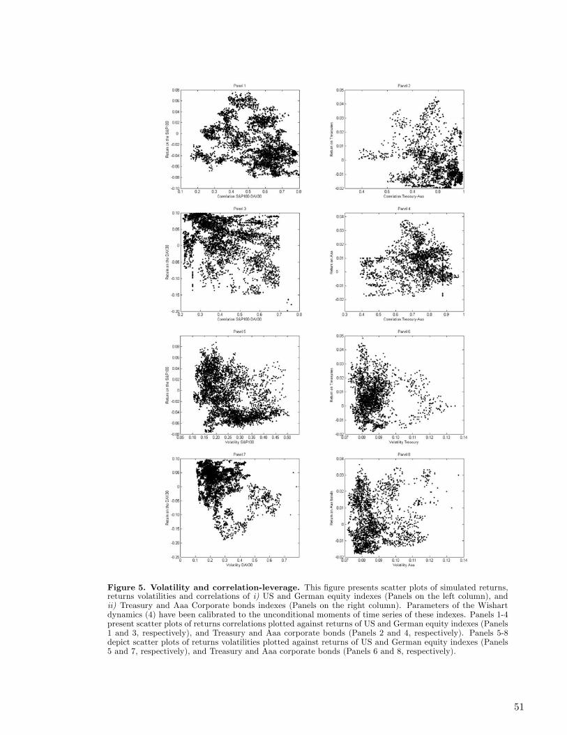
Figure 5. Volatility and correlation-leverage. This figure presents scatter plots of simulated returns,returns volatilities and correlations of i) US and German equity indexes (Panels on the left column), andii) Treasury and Aaa Corporate bonds indexes (Panels on the right column). Parameters of the Wishartdynamics (4) have been calibrated to the unconditional moments of time series of these indexes. Panels 1-4present scatter plots of returns correlations plotted against returns of US and German equity indexes (Panels1 and 3, respectively), and Treasury and Aaa corporate bonds (Panels 2 and 4, respectively). Panels 5-8depict scatter plots of returns volatilities plotted against returns of US and German equity indexes (Panels5 and 7, respectively), and Treasury and Aaa corporate bonds (Panels 6 and 8, respectively).

51

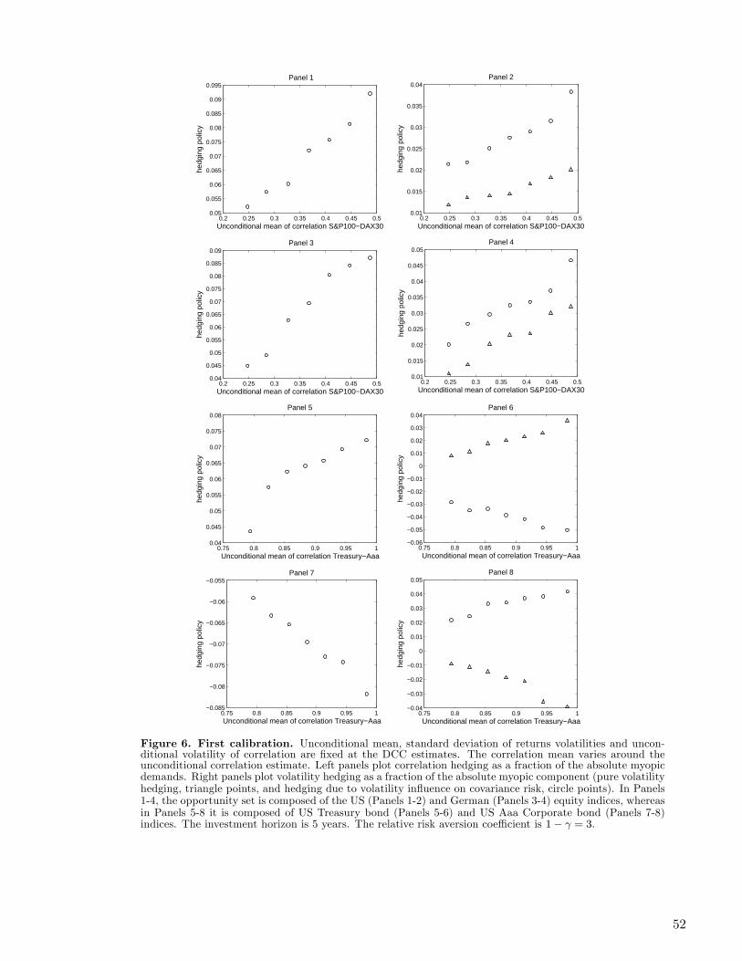
0.2 0.25 0.3 0.35 0.4 0.45 0.50.05

0.055

0.06

0.065

0.07

0.075

0.08

0.085

0.09

0.095

Unconditional mean of correlation S&P100−DAX30

hedg

ing

polic

y

Panel 1

0.2 0.25 0.3 0.35 0.4 0.45 0.50.01

0.015

0.02

0.025

0.03

0.035

0.04


hedg

ing

polic

y

Panel 2

0.2 0.25 0.3 0.35 0.4 0.45 0.50.04

0.045

0.05

0.055

0.06

0.065

0.07

0.075

0.08

0.085

0.09


hedg

ing

polic

y

Panel 3

0.2 0.25 0.3 0.35 0.4 0.45 0.50.01

0.015

0.02

0.025

0.03

0.035

0.04

0.045

0.05


hedg

ing

polic

y

Panel 4

0.75 0.8 0.85 0.9 0.95 10.04

0.045

0.05

0.055

0.06

0.065

0.07

0.075

0.08

Unconditional mean of correlation Treasury−Aaa

hedg

ing

polic

y

Panel 5

0.75 0.8 0.85 0.9 0.95 1−0.06

−0.05

−0.04

−0.03

−0.02

−0.01

0

0.01

0.02

0.03

0.04


hedg

ing

polic

yPanel 6

0.75 0.8 0.85 0.9 0.95 1−0.085

−0.08

−0.075

−0.07

−0.065

−0.06

−0.055


hedg

ing

polic

y

Panel 7

0.75 0.8 0.85 0.9 0.95 1−0.04

−0.03

−0.02

−0.01

0

0.01

0.02

0.03

0.04

0.05


hedg

ing

polic

y

Panel 8

Figure 6. First calibration. Unconditional mean, standard deviation of returns volatilities and uncon-ditional volatility of correlation are fixed at the DCC estimates. The correlation mean varies around theunconditional correlation estimate. Left panels plot correlation hedging as a fraction of the absolute myopicdemands. Right panels plot volatility hedging as a fraction of the absolute myopic component (pure volatilityhedging, triangle points, and hedging due to volatility influence on covariance risk, circle points). In Panels1-4, the opportunity set is composed of the US (Panels 1-2) and German (Panels 3-4) equity indices, whereasin Panels 5-8 it is composed of US Treasury bond (Panels 5-6) and US Aaa Corporate bond (Panels 7-8)indices. The investment horizon is 5 years. The relative risk aversion coefficient is 1− γ = 3.

52

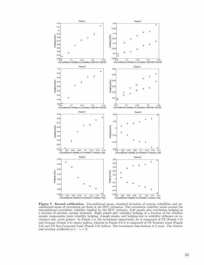
0.05 0.1 0.15 0.2 0.250.02

0.03

0.04

0.05

0.06

0.07

0.08

0.09

0.1

0.11

0.12

Unconditional volatility of correlation S&P100−DAX30

hedg

ing

polic

y

Panel 1

0.05 0.1 0.15 0.2 0.250.005

0.01

0.015

0.02

0.025

0.03

0.035

0.04


hedg

ing

polic

y

Panel 2

0.05 0.1 0.15 0.2 0.250.02

0.03

0.04

0.05

0.06

0.07

0.08

0.09

0.1


hedg

ing

polic

y

Panel 3

0.05 0.1 0.15 0.2 0.250

0.01

0.02

0.03

0.04

0.05

0.06


hedg

ing

polic

y

Panel 4

0.02 0.04 0.06 0.08 0.1 0.12 0.14 0.160.01

0.02

0.03

0.04

0.05

0.06

0.07

0.08

0.09

Unconditional volatility of correlation Treasury−Aaa

hedg

ing

polic

y

Panel 5

0.02 0.04 0.06 0.08 0.1 0.12 0.14 0.16−0.06

−0.04

−0.02

0

0.02

0.04


hedg

ing

polic

yPanel 6

0.02 0.04 0.06 0.08 0.1 0.12 0.14 0.16−0.09

−0.08

−0.07

−0.06

−0.05

−0.04

−0.03

−0.02


hedg

ing

polic

y

Panel 7

0.02 0.04 0.06 0.08 0.1 0.12 0.14 0.16−0.04

−0.03

−0.02

−0.01

0

0.01

0.02

0.03

0.04

0.05


hedg

ing

polic

y

Panel 8

Figure 7. Second calibration. Unconditional mean, standard deviation of returns volatilities and un-conditional mean of correlation are fixed at the DCC estimates. The correlation volatility varies around theunconditional correlation volatility implied by the DCC estimate. Left panels plot correlation hedging asa fraction of absolute myopic demands. Right panels plot volatility hedging as a fraction of the absolutemyopic components (pure volatility hedging, triangle points, and hedging due to volatility influence on co-variance risk, circle points). In Panels 1-4, the investment opportunity set is composed of US (Panels 1-2)and German (Panels 3-4) equity indices, whereas in Panels 5-8 it is composed of US Treasury bond (Panels5-6) and US Aaa Corporate bond (Panels 7-8) indices. The investment time-horizon is 5 years. The relativerisk aversion coefficient is 1− γ = 3.

53

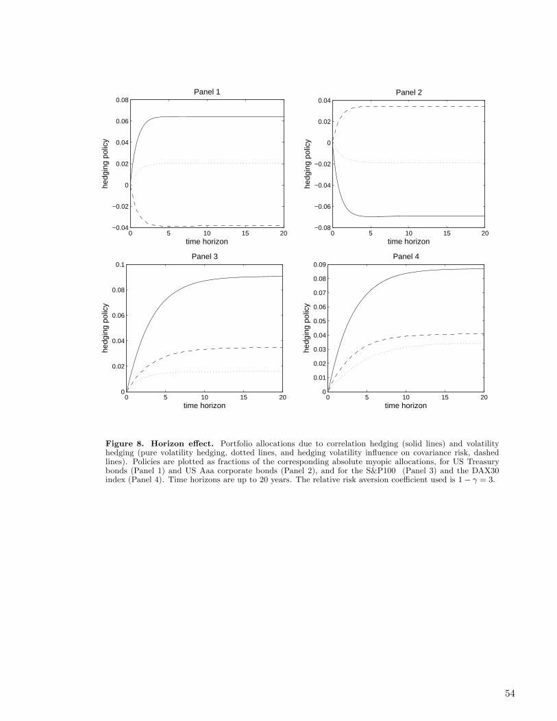
0 5 10 15 20−0.04

−0.02

0

0.02

0.04

0.06

0.08

time horizon

hedg

ing

polic

y

Panel 1

0 5 10 15 20−0.08

−0.06

−0.04

−0.02

0

0.02

0.04

time horizon

hedg

ing

polic

y

Panel 2

0 5 10 15 200

0.02

0.04

0.06

0.08

0.1

time horizon

hedg

ing

polic

y

Panel 3

0 5 10 15 200

0.01

0.02

0.03

0.04

0.05

0.06

0.07

0.08

0.09

time horizon

hedg

ing

polic

y

Panel 4

Figure 8. Horizon effect. Portfolio allocations due to correlation hedging (solid lines) and volatilityhedging (pure volatility hedging, dotted lines, and hedging volatility influence on covariance risk, dashedlines). Policies are plotted as fractions of the corresponding absolute myopic allocations, for US Treasurybonds (Panel 1) and US Aaa corporate bonds (Panel 2), and for the S&P100 (Panel 3) and the DAX30index (Panel 4). Time horizons are up to 20 years. The relative risk aversion coefficient used is 1− γ = 3.

54

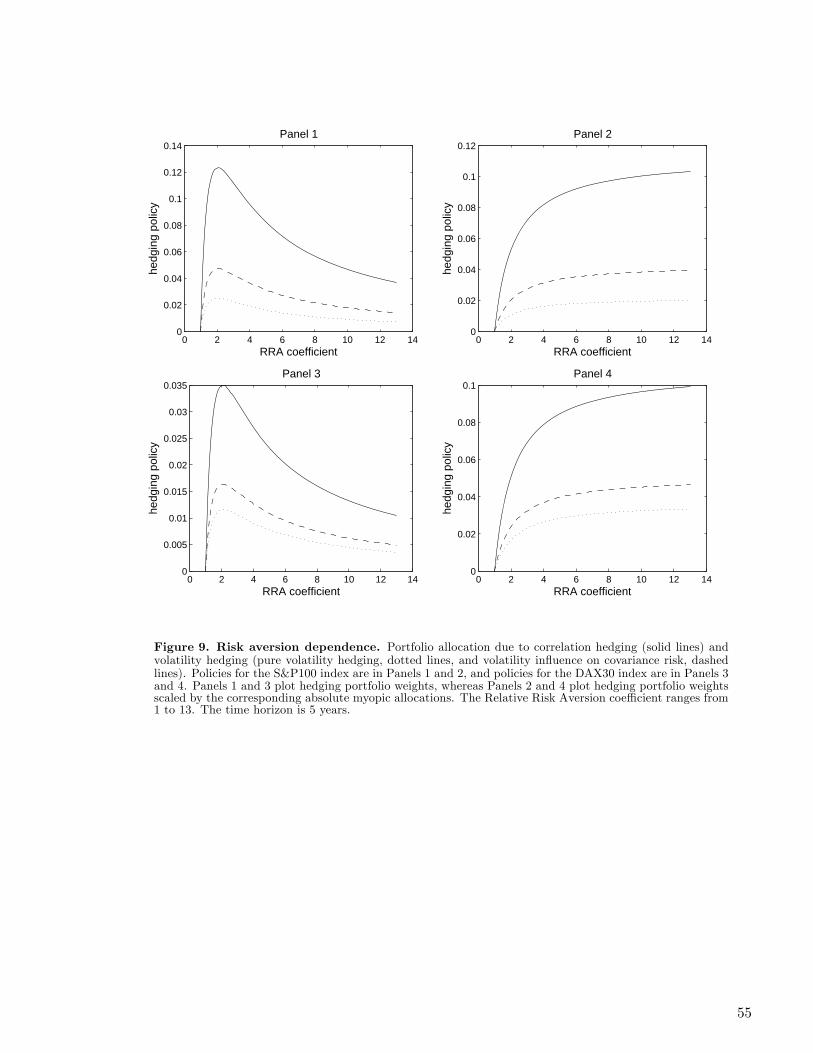
0 2 4 6 8 10 12 140

0.02

0.04

0.06

0.08

0.1

0.12

0.14

RRA coefficient

hedg

ing

polic

y

Panel 1

0 2 4 6 8 10 12 140

0.02

0.04

0.06

0.08

0.1

0.12

RRA coefficient

hedg

ing

polic

y

Panel 2

0 2 4 6 8 10 12 140

0.005

0.01

0.015

0.02

0.025

0.03

0.035

RRA coefficient

hedg

ing

polic

y

Panel 3

0 2 4 6 8 10 12 140

0.02

0.04

0.06

0.08

0.1

RRA coefficient

hedg

ing

polic

y

Panel 4

Figure 9. Risk aversion dependence. Portfolio allocation due to correlation hedging (solid lines) andvolatility hedging (pure volatility hedging, dotted lines, and volatility influence on covariance risk, dashedlines). Policies for the S&P100 index are in Panels 1 and 2, and policies for the DAX30 index are in Panels 3and 4. Panels 1 and 3 plot hedging portfolio weights, whereas Panels 2 and 4 plot hedging portfolio weightsscaled by the corresponding absolute myopic allocations. The Relative Risk Aversion coefficient ranges from1 to 13. The time horizon is 5 years.

55

0.01 0.02 0.03 0.04 0.05−0.06

−0.04

−0.02

0

0.02

0.04

0.06

0.08

0.1

short interest rate

hedg

ing

polic

y

Panel 1

0.01 0.02 0.03 0.04 0.05−0.08

−0.06

−0.04

−0.02

0

0.02

0.04

short interest rate

hedg

ing

polic

y

Panel 2

0.01 0.02 0.03 0.04 0.050.01

0.02

0.03

0.04

0.05

0.06

0.07

0.08

0.09

0.1

short interest rate

hedg

ing

polic

y

Panel 3

0.01 0.02 0.03 0.04 0.050.01

0.02

0.03

0.04

0.05

0.06

0.07

0.08

0.09

short interest rate

hedg

ing

polic

y

Panel 4

Figure 10. Dependence on calibrated λ. Portfolio allocation due to correlation hedging (solid lines) andvolatility hedging (pure volatility hedging, dotted lines, and volatility influence on covariance risk, dashedlines) as the calibrated parameter λ changes for increasing interest rate. Policies for US Treasury bonds andAaa Corporate bonds are in Panels 1 and 2, respectively. Policies for the S&P100 index and the DAX30index are in Panels 3 and 4. The Relative Risk Aversion coefficient is 3 and the time horizon is 5 years.

56

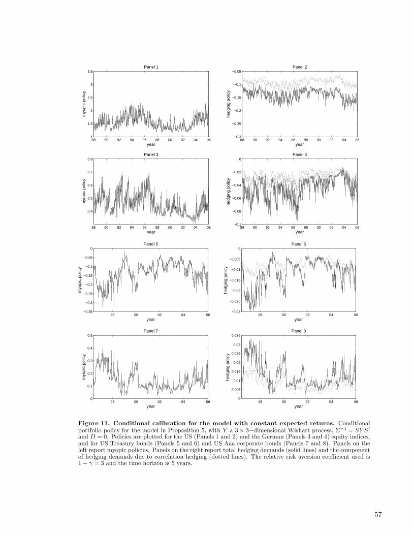
88 90 92 94 96 98 00 02 04 061

1.5

2

2.5

3

3.5

year

myo

pic

polic

y

Panel 1

88 90 92 94 96 98 00 02 04 06−0.3

−0.25

−0.2

−0.15

−0.1

−0.05

year

hedg

ing

polic

y

Panel 2

88 90 92 94 96 98 00 02 04 06

0.4

0.5

0.6

0.7

0.8

year

myo

pic

polic

y

Panel 3

88 90 92 94 96 98 00 02 04 06−0.1

−0.08

−0.06

−0.04

−0.02

0

yearhe

dgin

g po

licy

Panel 4

98 00 02 04 06−0.35

−0.3

−0.25

−0.2

−0.15

−0.1

−0.05

0

myo

pic

polic

y

Panel 5

year98 00 02 04 06

−0.03

−0.025

−0.02

−0.015

−0.01

−0.005

0Panel 6

year

hedg

ing

polic

y

98 00 02 04 060

0.1

0.2

0.3

0.4

0.5

myo

pic

polic

y

Panel 7

year98 00 02 04 06

0

0.005

0.01

0.015

0.02

0.025

0.03

0.035Panel 8

year

hedg

ing

polic

y

Figure 11. Conditional calibration for the model with constant expected returns. Conditionalportfolio policy for the model in Proposition 5, with Y a 3× 3−dimensional Wishart process, Σ−1 = SY S0

and D = 0. Policies are plotted for the US (Panels 1 and 2) and the German (Panels 3 and 4) equity indices,and for US Treasury bonds (Panels 5 and 6) and US Aaa corporate bonds (Panels 7 and 8). Panels on theleft report myopic policies. Panels on the right report total hedging demands (solid lines) and the componentof hedging demands due to correlation hedging (dotted lines). The relative risk aversion coefficient used is1− γ = 3 and the time horizon is 5 years.

57

Correlation Risk and Optimal Portfolio Choice ANNUAL... · Correlation Risk and Optimal Portfolio...

Documents

Transcript of Correlation Risk and Optimal Portfolio Choice ANNUAL... · Correlation Risk and Optimal Portfolio...