Corporate Life-Cycle Dynamics of Cash Holdings ANNUAL MEETINGS/2016...Corporate Life-Cycle Dynamics...
39
Corporate Life-Cycle Dynamics of Cash Holdings Wolfgang Drobetz, Michael Halling, and Henning Schröder * Abstract This paper shows that the corporate life-cycle is an important dimension for the dynamics and valua- tion of cash holdings. Our results indicate that firms’ cash policies are markedly interacted with their strategy choices. While firms in early stages and post-maturity stages hold large amounts of cash, cash ratios decrease when firms move towards maturity. Much of this variation in cash holdings is attribut- able to a changing demand function for cash over the different life-cycle stages. Trade-off and peck- ing order motives are of different importance for cash policies dependent on a firm’s life-cycle stage. An additional dollar in cash is highly valuable for introduction and growth firms, while a dollar in cash adds, on average, less than a dollar in market value for firms in later life-cycle stages, most likely due to increasing agency problems. Most of the dynamics in cash holdings are observed at life-cycle transition points rather than during the different life-cycle stages. Finally, the secular trend in cash holdings seems strongly attributable to increases in cash in the introduction and the decline stage. Keywords: Life-cycle, cash holdings, value of cash JEL Classification Codes: G30, G32, M10 * Drobetz ([email protected]) and Schroeder ([email protected]) are with the Finance Department, University of Hamburg. Halling ([email protected]) is with the Stockholm School of Economics and the Swedish House of Finance. We thank Laurent Bach, Bo Becker, Igor Cunha, Claudia Custodio, Ralf Elsas (discussant), Miguel Ferreira, Daniel Rettl, Alex Stomper and Jin Yu (discussant) for helpful suggestions. We also thank participants of the 2015 conference in honor of Josef Zechner, the 2015 conference of the German Finance Association, the 2015 IFABS Corporate Finance conference in Oxford, and seminar participants at Nova School of Business and Economics, Humboldt University Berlin, and the Stock- holm School of Economics for their comments.
Transcript of Corporate Life-Cycle Dynamics of Cash Holdings ANNUAL MEETINGS/2016...Corporate Life-Cycle Dynamics...

Corporate Life-Cycle Dynamics
of Cash Holdings
Wolfgang Drobetz, Michael Halling, and Henning Schröder*
Abstract
This paper shows that the corporate life-cycle is an important dimension for the dynamics and valua-
tion of cash holdings. Our results indicate that firms’ cash policies are markedly interacted with their
strategy choices. While firms in early stages and post-maturity stages hold large amounts of cash, cash
ratios decrease when firms move towards maturity. Much of this variation in cash holdings is attribut-
able to a changing demand function for cash over the different life-cycle stages. Trade-off and peck-
ing order motives are of different importance for cash policies dependent on a firm’s life-cycle stage.
An additional dollar in cash is highly valuable for introduction and growth firms, while a dollar in
cash adds, on average, less than a dollar in market value for firms in later life-cycle stages, most likely
due to increasing agency problems. Most of the dynamics in cash holdings are observed at life-cycle
transition points rather than during the different life-cycle stages. Finally, the secular trend in cash
holdings seems strongly attributable to increases in cash in the introduction and the decline stage.
Keywords: Life-cycle, cash holdings, value of cash
JEL Classification Codes: G30, G32, M10
* Drobetz ([email protected]) and Schroeder ([email protected]) are
with the Finance Department, University of Hamburg. Halling ([email protected]) is with the Stockholm
School of Economics and the Swedish House of Finance. We thank Laurent Bach, Bo Becker, Igor Cunha,
Claudia Custodio, Ralf Elsas (discussant), Miguel Ferreira, Daniel Rettl, Alex Stomper and Jin Yu (discussant)
for helpful suggestions. We also thank participants of the 2015 conference in honor of Josef Zechner, the 2015
conference of the German Finance Association, the 2015 IFABS Corporate Finance conference in Oxford, and
seminar participants at Nova School of Business and Economics, Humboldt University Berlin, and the Stock-
holm School of Economics for their comments.

2
I. Introduction
The dynamics and valuations of corporate cash holdings have received a lot of attention in
the corporate finance literature. Motives, such as precautionary saving, competitive pressure
or refinancing risk, are suggested to rationalize observed cash levels. Agency costs and tax
issues are important costs associated with holding cash. However, little consensus has been
reached about the relative importance of and the interplay between these concepts. We argue
in this paper that an important dimension has been missing from the discussion, namely the
corporate life-cycle.1 The goal of our paper is to close this gap.
The notion of a corporate life-cycle is a highly complex and multi-dimensional concept.
Among other things, the economics literature connects production and investment behavior
(Jovanovic and MacDonald (1994)), experience and learning (Spence (1981)), and competi-
tion as well as market share (Wernerfelt (1985)) to the corporate life-cycle. Broadly speaking,
when we refer to the corporate life-cycle, we think about firms following different strategies
in different stages to deal with varying constraints and challenges. Therefore, our paper also
relates to the strand of the literature that links firms’ strategic decisions to financing choices
(see Parsons and Titman (2008) for an overview). In particular, the focus of our study is to
evaluate empirically and in the context for firms’ cash management whether the corporate
life-cycle matters.
The key challenge for the econometrician is to determine from observable data which life-
cycle stage a firm is in during a particular period of time. For this purpose, we follow Dickin-
son (2011), who developed and evaluated a mechanism to match firms to life-cycle stages
using the signs of cash-flows from various sources (i.e., operations, investments, and financ-
ing). Specifically, we distinguish five stages – introduction, growth, maturity, shake-out and
decline (see Gort and Keppler (1982)) – in this paper. An important conceptual advantage of
this classification is that it does not imply a strict sequence across the stages of the life-cycle
and, in contrast, allows firms to dynamically move back and forth between stages. This setup
1 The only exception we know of is a working paper, Dittmar and Duchin (2011), which looks at the interaction
between firm age (time since IPO), as a proxy for the life-cycle, and cash holdings. Our analysis differs substan-
tially in terms of methodology to identity life-cycle stages and empirical tests regarding the cash management of
firms.

3
allows us to study and distinguish a rich cross-section of transitions between life-cycle stages
in our empirical analysis.
Surprisingly, the literature is relatively silent regarding the importance of the corporate life-
cycle for corporate finance questions. Notable exceptions are DeAngelo, DeAngelo and Stulz
(2006), using retained earnings as proxy for the life-cycle stage, and DeAngelo, DeAngelo
and Stulz (2010), using years listed as proxy for the life-cycle stage. They find that firms’
payout policies are consistent with a life-cycle theory of the firm (see also Banyi and Kahle
(2014)). Bulan and Yan (2010) study the link between the pecking order theory and the cor-
porate life-cycle. They consider only two stages – the “growth” stage is defined as the first 6
years post-IPO and the “maturity” stage is defined as the consecutive six-year period follow-
ing a dividend initiation. Finally and most closely related to our paper, Dittmar and Duchin
(2011) study the dynamics of cash using firm age (years since the IPO) as a measure of the
corporate life-cycle.
Our main results are as follows. Levels of observed and target cash, determinants of target
cash, adjustment speeds, and the value of cash vary substantially across life-cycle stages.
These results suggest that firms in different life-cycle stages follow different motives in their
cash policies. For example, we find that firms in life-cycle stages 1 (“introduction”) and 5
(“decline”) actively manage their cash holdings towards target levels and, given their pro-
nounced levels of financial constraints and low correlations between operating income and
investment opportunities (Acharya, Almeida, and Campello (2007)), use cash as a hedging
instrument. In contrast, firms in the “maturity” life-cycle stage put less weight on target cash
holdings but adjust cash holdings in response to the fortunes of the company (i.e., they follow
the financing hierarchy model).
We also study secular trends in the dynamics of aggregate cash holdings per life-cycle stage.
Bates, Kahle and Stulz (2009) document a steady increase in cash holdings over time. We
find that average/median cash holdings have increased over time for all life-cycle stages but
to varying degrees. The strongest increases in cash holdings are observed for firms in the “in-
troduction” and the “decline” stage.

4
Life-cycle stages also play an important role in determining the valuation of cash. As one
would expect, we find that an additional dollar in cash is highly valuable in the “growth”
stage. However, a dollar in cash adds, on average, less than a dollar in market value for firms
in life-cycle stages 4 (“shake-out”) and 5 (“decline”), most likely due to pronounced agency
costs. Interestingly, the value of an additional dollar of cash is much lower for firms in life-
cycle stage 5 than in life-cycle stage 1. This is surprising given that our analysis of target cash
levels (and speeds of adjustment) suggests that firms in life-cycle stages 1 and 5 follow rela-
tively similar cash policies. It thus seems that the market evaluates the motives to hold cash
very differently depending on the stage of the life-cycle that a firm is in.
Finally, and most importantly, we find that transitions between life-cycle stages matter a lot.
In particular, we find substantial variation in median cash levels in the final year of a given
life-cycle stage depending on the target life-cycle stage in the subsequent year. Similarly, we
observe pronounced differences in relative changes of cash holdings during transition years.
For example, the median firm in the “introduction” stage has cash holdings of 6.7% in the
year before progressing to the “growth” stage and increases its cash holdings by 11.3% in the
following year. In contrast, the median firm in the “introduction” stage that moves on to the
“decline” stage shows cash holdings of 40.8% and marginally reduces them by 0.5% in the
following year. We also find that the market takes future life-cycle stages into consideration
when evaluating additional dollars in cash. For example, the value of an additional dollar in
cash is 1.43 (0.56) for firms in the “maturity” stage that are transiting to the “introduction”
(“shake-out”) stage in the following year.
An important caveat, however, applies to the current set of results. While our analysis sug-
gests an important role for the corporate life-cycle on top of standard firm characteristics in
explaining cash management policies, we are not able to establish causality, i.e., we do not
know whether strategic decisions drive financing decisions or vice versa. In the end, it seems
not unlikely that both are determined contemporaneously.
The paper is organized as follows. In section 2 we explain the methodology to assign firms to
life-cycle stages and provide some motivation for why we expect the corporate-life-cycle to

5
matter for cash management. Section 3 describes the data, and section 4 summarizes our em-
pirical results. Section 5 concludes.
II. Measuring the Corporate Life-Cycle
Although the life-cycle theory of the firm has been of enduring interest to researchers in theo-
retical and empirical economics, there exists neither a unique life-cycle model nor a consen-
sus on the definition of corporate life-cycle stages. Proposed models differ in terms of their
aggregation level and the number of life-cycle stages. The theoretical literature proposes
three-stage, four-stage, or five-stage models that focus primarily on a description of the prod-
uct life-cycle, while viewing the firm as an aggregation of the single product cycles. Overall,
most models agree about the stages introduction, growth, and maturity. In addition, higher
order models also include post-maturity stages.
From the empirical perspective, current research further lacks a consensus on how to identify
each life-cycle stage. Empirical applications in financial research, so far, have been dominat-
ed by univariate approaches to map the life-cycle of the firm. Both size and age, but also the
earned/contributed capital mix, are common proxies for a firm’s current life-cycle stage.
However, the implicit assumption when using these measures is that a firm moves monoton-
ically from its introduction to maturity, staying there until ‘death’. This again implies that
such measures fail to cover corporate reinvention and restructuring scenarios, since they do
not allow firms to enter back into the introduction or growth stage once they have reached
maturity. An important advantage of the classification of life-cycle stages employed in this
study is that firms do not have to run through the individual stages sequentially. Instead, they
can basically jump back and forth in any arbitrary way. The following sections describe the
applied measure and its implementation in detail.
A. Formulation of the Life-Cycle Measure
To incorporate post-maturity stages, we adapt a five-stage life-cycle measure recently devel-
oped by Dickinson (2011). Following Gort and Klepper (1982), Dickinson (2011) defines (1)
introduction, (2) growth, (3) maturity, (4) shake-out, and (5) decline as the relevant life-cycle
stages. Her life-cycle identification strategy is based on the proposition that corporate cash

6
flows capture the financial outcome of the distinct life-cycle stages, so that each stage has a
characteristic pattern of net cash flows, i.e., a stage-specific combination of operating cash
flow, investing cash flow, and financing cash flow. The idea behind is that the combination of
cash flow patterns represents a firm’s resource allocation and operational capability interact-
ed with its strategy choices. Abstracting from the actual level, each of the three types of cash
flows can take a positive or negative sign. Combining the three cash flow signs, results in
eight possible combinations of potentially observable cash flow patterns, which are mapped
into life-cycle theory in order to derive an empirically applicable life-cycle classification. In
contrast to univariate metrics, this ‘cash flow pattern proxy’ is based on the entire financial
information set available at each financial statement date. Following Dickinson (2011), Table
I provides an overview of the eight possible cash flow combinations and the resulting life-
cycle classification scheme.
[Insert Table I here]
Introduction (LC-1): As a consequence of lacking established customers, unexploited econ-
omies of scale, and a deficit of knowledge about costs and revenues (Jovanovic (1982)), in-
troduction firms typically suffer from negative net cash flows from operating activities. On
the other hand, they are expected to make large investments to provide or renew the basis for
its operating activities and to exploit existing growth opportunities, leading to negative in-
vesting cash flows. Given that introduction firms arguably do not possess sufficient capital
resources to continuously finance outflows from operations and investment, they need to rely
on external financing, i.e., financing cash flows are expected to be positive.
Growth (LC-2): In contrast to introduction-stage firms, growth-stage firms maximize their
profit margins by optimizing their investment activity and increasing operational efficiency
(Spence (1977, 1979, 1981), Wernerfelt (1985)), so that operating cash flows are expected to
become positive. Similar to the preceding life-cycle stage, investment cash flows are still
expected to be significantly negative. Although cash inflows from operations may be used
cover the continuing investment activity, growth firms typically require further external fi-
nancing to maintain high investment capacity.

7
Maturity (LC-3): Entering maturity, firms are expected to further increase efficiency. Both
maximized profit margins and the large customer base of mature firms provide high operating
cash flows. By definition, mature firms have exhausted their positive net present value pro-
jects, so that they have fewer investment opportunities. Therefore, investments are reduced
relative to the preceding stages. However, mature firms are expected to maintain capital, still
resulting in negative cash flows from investing during the maturity stage. Both the high oper-
ational profitability and the lack of investment opportunities minimize the need for external
financing. Given the expected financial surplus, mature firms start to service debt and/or dis-
tribute cash to shareholders leading to negative financing cash flows.
Shake-out (LC-4): Firms entering the shake-out stage exhibit declining or negative growth
rates. Arguably, this leads to declining prices (Wernerfelt (1985)), while re-increasing ineffi-
ciencies attributable to larger firm size or distress related phenomena lead to an extended cost
structure over the life-cycle. Both effects result in decreasing (or negative) operating cash
flows. Similar to mature firms, shake-out firms may continue to invest for maintenance rea-
sons. On the other hand, they may liquidate assets to service existing debt obligations and to
support operations, i.e., investing cash flows may either be positive or negative. The same
holds for financing cash flows. Although shake-out firms may still be able to distribute cash
to shareholders, they may also rely on external financing to cover capital maintenance or def-
icits from operations.2
Decline (LC-5): Decline firms suffer from a deteriorating dilution of earning relative to the
shake-out stage. Increased costs of financial distress are expected to further depress corporate
results, so that most likely decline firms exhibit negative operating cash flows. In contrast,
investment cash flows are expected to be positive. By definition decline firms lack appropri-
ate investment opportunities, but are likely to liquidate assets to support operations rather
2 Life-cycle stage 4, shake-out, is associated with 3 combinations of operating, investing and financing cash-
flows. Empirically, we find that pattern #6 in Table I – positive operating, positive investing and negative fi-
nancing cash-flows – is by far the most frequent one with, on average, more than 80% of all firms being classi-
fied to be in shake-out stage featuring this pattern.
8
than expanding their capital budgets. Depending on the deficit (surplus) after investments,
decline firms will have positive (negative) financing cash flows.3
B. Implementation of the Life-Cycle Proxy
Following Table I, the combination of a firm’s net operating, investing, and financing cash
flows provide the firm’s life-cycle classification at each financial statement date. In order to
reduce the impact of single-year effects, we use three-year moving averages of each cash
flow type rather than fiscal year-end values to obtain the final life-cycle classification. At this
point we deviate from Dickinson (2011), who uses fiscal year-end cash flow data as reported
by the firm to implement her life-cycle proxy. The applied correction of the measure controls
for non-fundamental life-cycle classification changes of firms with cash flows around zero. In
such cases, cash flows may change signs due to single-year effects that are not related to the
operational capability or strategy choice of the firm, resulting in a life-cycle classification
possibly providing misleading information on the actual life-cycle stage of the firm. Though
the choice of using a three-year moving average is ad hoc to a certain extent, it seems to be a
reasonable way to deal with single-year effects. Eventually, using a moving average-based
classification does not substantially affect the distributional characteristics of the life-cycle
proxy. However, it slightly increases the average dwelling time per life-cycle stage relative to
the Dickinson (2011) classification. Section IV.B provides a brief comparison of transition
probabilities implied by both implementations.
One might worry that there is a mechanical link between this cash-flow based procedure to
separate life-cycle stages and our variable of interest, cash holdings. While there is obviously
an important difference between flow and stock variables, it is also important to reemphasize
that we only condition on the signs of cash-flows (and their specific patterns across the three
sources) rather than their magnitudes. Importantly, all stages of the life-cycle are identified
by a combination of positive and negative cash-flows, and thus no stage is unambiguously
associated with a positive or negative total cash-flow shock.
3 The decline stage is associated with two different cash-flow patterns, which both are empirically frequently
observed. On average, 60% of all firms classified to be the decline stage have negative operating, positive in-
vesting and positive financing cash-flows (pattern #7).
9
III. Data
For our empirical analyses, we obtain annual accounting data of U.S. incorporated industrial
firms (active and inactive) from the WRDS merged CRSP/Compustat files for the period
1989 through 2013. 4
We explicitly exclude firms with SIC codes inside the ranges 4900–
4999 (utilities) and 6000–6999 (financial firms) that operate in regulated markets and whose
cash holding behavior may be driven by special factors. We initially require that firms have
non-missing data on total asset (AT) and sales (SALE) to be included in the sample and we
exclude firms with book assets below 1 million USD.
Our central figure of interest is the cash balance of the firm measured as cash and equivalents
(CHE) scaled by total assets (AT). To construct the lifecycle proxy for each firm-year, we
follow the classification scheme in Table I. Specifically, we use the past three-year moving
average of (i) net cash flow from operating activities (OANCF), (ii) net cash flow from in-
vesting activities (IVNCF), and (iii) net cash flow from financing activities (FINCF) instead
of the plain fiscal year-end values. Detailed information on the construction principles of oth-
er variables used in this study are provided in Appendix A. Our final sample comprises
77,377 firm-years with non-missing data for cash and the life-cycle classification (introduc-
tion: 12,963; growth: 26,338; maturity: 27,814, shake-out: 4,849; decline: 5,413).
IV. Empirical Results
In this section, we summarize the empirical results. First, we discuss summary statistics fo-
cusing on the patterns of firm characteristics over the corporate life-cycle. We also discuss
transition probabilities between life-cycle stages and look at the dynamics of aggregate cash
levels per life-cycle over time. Second, we report detailed results for the drivers of cash hold-
ings of firms and run a horse race between the trade-off theory and the pecking order theory
to understand how firms manage their cash holdings. Third, we analyze the marginal value of
an additional dollar in cash. In all these discussions, the focus is on a comparison of results
4 Consistent statement of cash flow data for all U.S. companies in Compustat is only available subsequent to the
adoption of the Statement of Financial Accounting Standards #95 (effective for fiscal years ending July 15, 1988
onwards).

10
across firms in different life-cycle stages, as this is the key contribution of the paper. Full
sample estimates are usually included to ensure comparability to the existing literature.
A. Descriptive Statistics
First, we examine the variation in corporate characteristics over the life-cycle. Table II re-
ports summary statistics for our full sample and for firms in individual life-cycle stages.5
Most importantly, cash holdings exhibit a U-shaped pattern, with the largest (lowest) average
level of cash holdings observed for firms in life-cycle stages 5 and 3, amounting to 38.2%
and 13.7% respectively. While leverage measured at book or market values does not show a
distinct pattern across the corporate life-cycle, short-term debt mimics the U-shape of cash
holdings, albeit to a less extreme extent. These patterns are consistent with Acharya, Da-
vydenko, and Strebulaev (2012), who show that a conservative cash policy (i.e., higher cash
levels) is more likely to be pursued by a firm that finds itself close to distress. As a result,
larger cash holdings are empirically associated with higher, not lower, levels of credit risk.
[Insert Table II here]
If we analyze variables that have been used in the prior literature as univariate proxies for a
firm’s life-cycle, we observe similarities, but also notable differences. Age, for example,
shows a hump-shaped pattern indicating that, on average, firms in later life-cycle stages (i.e.,
“decline” and “shakeout” or LC-4 and LC-5) are younger and not older than mature firms
(i.e., firms in LC-3). Not surprisingly, this suggests that age as a “linear” indicator of firm
life-cycle is not very sensible.
Somewhat similar patterns are observed for size, retained earnings, and payout measures.
They do not increase monotonically across life-cycle stages, but follow hump shapes. Over-
all, it seems that our classification of life-cycles cannot be easily replicated by using any of
the standard, univariate measures employed in the literature before.
In terms of other firm characteristics, we observe intuitive patterns across the board. Many
variables such as tangibility, operating income, net working capital and capital expenditures
5 In the following discussion, we focus on average values. Note, however, that all patterns described also hold
for median values.

11
feature hump shapes, reaching their maximum values either for firms in LC-2 or LC-3 and
decreasing towards the earlier and later life-cycle stages. In contrast, variables such as mar-
ket-to-book ratios, R&D expenses, equity issuances, and financing deficits exhibit U-shaped
patterns. Measures of financial constraints feature both patterns depending on how they are
defined; however, they all suggest that firms in earlier and later life-cycle stages are more
constrained than mature firms.
Table II also reports standard deviations of firm characteristics across LC-stages. In the ma-
jority of cases, we observe a U-shaped pattern suggesting that the set of mature firms is most
homogenous. For some important variables, such as size, age or industry market share, how-
ever, we find the largest standard deviations among mature firms.
Finally, we take a look at secular trends in the dynamics of aggregate cash holdings for each
life-cycle stage. Bates, Kahle and Stulz (2009) document that cash holdings have increased
substantially over the last thirty years. They relate this pattern to an increase in the riskiness
of firms’ cash-flows and similar trends in other firm characteristics, concluding that the pre-
cautionary saving motive plays an important role in explaining these dynamics. Figure I plots
average and median cash holdings over time for firms in different life-cycle stages.6 Most
importantly, we find that this increase in cash holdings is driven to a large extent by firms in
LC-1 and LC-5. These firms raised their cash levels three to four times during our sample
period. In contrast, average/median cash holdings have increased much less for firms in other
life-cycle stages.
[Insert Figure I here]
Another interesting and surprising result is that cash holdings were very similar across life-
cycle stages early on in our sample. During the late 80ties and early 90ties median cash hold-
ings, for example, varied between 5% and 10% across life-cycle stages. In contrast, at the end
of our sample period this variation covers the range of 10% to 50%. This suggests that the
interaction between the corporate life-cycle and cash management has changed dramatically.
6 In unreported robustness tests, we replicated Figure I for a sample in which we dropped all firm-year observa-
tions in the five years following the IPO to avoid any confounding effects of the large inflow of cash due to the
share issuance. The patterns that we observe for secular trends per life-cycle stage are unaffected by this.
12
A somewhat related question is whether there have been any long-term trends in the distribu-
tion of firms across life-cycle stages. Figure II shows the proportions of firms in each life-
cycle stage over time using equal and value weighting. As one would expect, firms tend to
concentrate in LC-2 and LC-3. Interestingly, however, there has been a persistent shift to-
wards firms in the “maturity” life-cycle stage after 2000, at least if we use value weighting.
Another interesting observation is that the frequency of firms in the “introduction” phase has
declined over time reaching its minimum of less than 10% during the most recent years. Fi-
nally, it is interesting to point out that the graphs do not exhibit any notable business cycle
effects.
[Insert Figure II here]
B. Dynamics of Cash Around Life-Cycle Transitions
An important advantage of the classification of life-cycle stages employed in our study is that
firms do not have to run through the individual stages sequentially. Instead, they can basically
jump back and forth in any arbitrary way. Overall, the average period a firm stays in a specif-
ic life-cycle stage is 2.8 years, but it slightly differs across life-cycle stages (introduction: 2.3
years; growth: 2.9 years; maturity: 3.4 years; shake-out: 2.0 years; decline: 2.2 years).7
Table III reports the corresponding transition probabilities across life-cycle stages. Most im-
portantly, it shows that firms have a tendency to stay in a life-cycle stage for a few years. For
example, the “maturity” life-cycle stage seems to be the stickiest stage, as one would expect:
52% of the firms that are in this stage at time t continue to stay in this stage for five years. In
contrast, the “shake-out” stage is the one from which firms exit most quickly – only 12.6%
stay in this stage for five years. Importantly, our classification does not imply that firms
change their life-cycle stage every year, which would not have been very realistic.
[Insert Table III here]
7 The lifecycle classification applied throughout this study deviates from the original classification proposed by
Dickinson (2011) in that we use three-year moving averages instead of fiscal year-end values of the cash flow
types to obtain these lifecycle proxies. Using the Dickinson (2011) classification, the average period that a firm
stays in a specific stage decreases to 1.8 years (introduction: 1.65 years; growth: 1.86 years; maturity: 1.98
years; shake-out: 1.77 years; decline: 1.63 years).

13
In terms of transitions across life-cycle stages, we find that transition probabilities are highest
for neighboring life-cycle stages, i.e., if firms switch, they tend to either progress to the next
life-cycle stage or drop back to the previous one. Again, this seems intuitive and provides
some comfort regarding our classification. Nevertheless, in some cases larger jumps across
various life-cycle stages are also observed. For example, a firm that is in LC-4 this year has a
10% chance of being in LC-2 next year (i.e., moving back from the “shake-out” stage to the
“growth” stage).
The focus of our study is on cash holdings and their dynamics for firms in different life-cycle
stages. While we have already noted that average cash levels follow a hump shape according
to Table II, Table IV provides a more detailed analysis focusing on median cash holdings
before transitions and subsequent changes in cash holdings. In this table, we focus on medi-
ans rather than averages, as changes in cash levels during life-cycle stages and around transi-
tions suffer from extreme, positive outliers.
[Insert Table IV here]
Most importantly, we observe in Panel A that firms have different levels of cash in the last
year of each stage depending on where they are moving to. For example, depending on where
a firm is moving to the median level of cash holdings in the last year in LC-1 varies between
2.7% (firms moving into LC-3 next year) and 40.8% (firms moving into LC-5). Interestingly,
these patterns mimic the U-shaped pattern that we observed for cash holdings in general, i.e.,
cash holdings tend to be highest in the last year of any LC-stage if the firm moves either into
the introduction or the decline stage. On the other hand, lowest pre-transition cash levels are
observed for firms changing into the maturity stage. The only exception are firms that are in
their last year of the maturity life-cycle stage.
Panel B of Table IV reports median relative cash changes immediately before transitions and
during life-cycle phases. Interestingly, but maybe not unexpectedly, the median changes in
cash levels during each life-cycle stage are zero (i.e., the diagonal elements of Panel B). This
pattern, however, changes if we focus on time periods immediately before transitions. For
example, irrespective of its current life-cycle stage (with the exception of firms in LC-5), the

14
median firm that switches to LC-1 next year reduces its cash holdings in the year of the tran-
sition. We find the largest (smallest) reduction for firms in LC-3 (LC-4) amounting to 19.4%
(2.8%). In contrast, the median firm emerging from LC-1 increases its cash holdings in the
year of the transition, except if it moves directly into life-cycle stage LC-5.
If we follow the median firm through the corporate life-cycle sequentially, we observe the
following changes in cash levels around transitions: a firm in LC-1 increases its cash level by
11.3% in the year of switching into the growth phase; it then only marginally raises the cash
level even further when moving on to LC-3, by 0.6%; surprisingly, it keeps increasing the
cash level by 8.3% when transitioning to LC-4 but then reduces it substantially, by 8.5%,
when changing into the decline phase. In general, the largest decreases in cash levels are ob-
served for firms switching back to earlier life-cycle stages, especially into the introduction
stage. Similarly, most pronounced increases are observed for transitions of firms into later
stages, especially the maturity and the shake-out stage.8
These results suggest that the corporate life-cycle and cash holdings are closely intertwined.
In a given life-cycle stage, firms are keeping their cash holdings rather stable, suggesting that
benefits and costs of cash do not vary much within a specific stage. However, around transi-
tions into later or earlier life-cycle stages, cash holdings change notably. As expected, cash
holdings increase when firms move through the life-cycle stages sequentially, i.e., become
more mature, until they enter the final, decline, stage. In contrast, firms tend to use up cash if
they ‘reinvent’ themselves and move back to earlier stages, such as introduction and growth.
C. Determinants of Cash over the Life-Cycle
The results up to this point already suggest that cash holdings and dynamics vary across the
corporate life-cycle. However, so far we have not controlled for other firm characteristics that
have been shown to affect cash policies. In a next step, we thus follow the literature (Opler et
al. (1999), Bates, Kahle and Stulz (2009), Harford, Klasa and Maxwell (2014), among others)
8 One might think that these dynamics are inconsistent with the U-shaped patterns described in Table II. This,
however, is not the case, as these results cannot be directly compared. Note that the dynamics in Table IV are
focusing on individual years within each stage (i.e., the first and the last year) and are conditioning on the target
life-cycle stage as well as the stage of origin.

15
and estimate target cash level regressions controlling for the standard set of firm characteris-
tics.
We model the cash-to-assets ratio as a function of net working capital scaled by total assets,
leverage (split into short-term debt scaled by total assets and long-term-debt scaled by total
assets,) firm size (measured as the natural logarithm of total assets in constant USD), market-
to-book assets, R&D expenses scaled by sales, capital expenditures scaled by total assets, a
dividend payer dummy variable (indicating whether a firm paid a dividend in a given year),
operating income scaled by total assets, median industry cash flow volatility, and acquisition
expenses scaled by total assets (see Appendix A for further details on the construction of
these variables). Table V shows the corresponding results. While column 2 (labeled “Full”)
shows results for the entire sample, the remaining five columns show the results if these re-
gressions are estimated separately for each life-cycle stage. All regression specifications in-
clude firm-fixed and year-fixed effects to control for unobserved heterogeneity across firms
and over time. All ratios are winsorized at the upper and lower one percentile to eradicate
errors and to mitigate the impact of outliers.
[Insert Table V here]
Looking at the results for the full sample, we find that they are consistent with the literature
(Opler et al. (1999), Bates, Kahle, and Stulz (2009), Harford, Klasa, and Maxwell (2014)). In
particular, coefficient signs and magnitudes fit well to previously reported values, indicating
that our sample is comparable to previously analyzed samples.
As a next step, we compare coefficients across columns 2 to 6 to investigate whether the cor-
porate life-cycle has any noticeable impact on these relations. We find strong evidence that
this is the case, as coefficients of several variables vary dramatically across firms in different
life-cycle stages. In what follows, we will discuss some of these life-cycle patterns in more
detail.
The link between short-term debt and cash holdings is a particularly interesting case. We find
negative coefficient estimates across the board, but the link is much less pronounced for firms
in LC-1 and LC-5. In the latter case, we do not even find any statistically significant link. In

16
contrast, in LC-2, LC-3, and to some extent LC-4, we find statistically highly significant and,
in absolute terms, large coefficient estimates. One interpretation of these results is that short-
term debt and cash levels seem to be substitutes for firms in LC-2, LC-3, and LC-4, while
they seem to be rather independent from each other in LC-1 and LC-5. Both cash holdings
and short-term debt show a U-shaped pattern across life-cycle stages in Table II, thus indicat-
ing that they both are important sources of funding for firms in LC-1 and LC-5.
This result seems to be consistent with Acharya, Almeida, and Campello (2007), who show
theoretically and empirically that cash is different from negative debt for firms facing financ-
ing frictions and having hedging needs, i.e., firms in life-cycle stages LC-1 and LC-5. In fact,
Table II confirms that standard measures of financial constraints peak for firms in LC-1 and
LC-5. Moreover, it shows that operating income is lowest and market-to-book ratios are
highest for these firms.9 Therefore, it seems reasonable to assume that these firms face low
correlations between operating income and investment opportunities.
Firm size is often used as a proxy for information asymmetries (i.e., large firms being less
exposed to information asymmetries), and the negative coefficient usually estimated in such
regressions is consistent with this interpretation. Nevertheless, we do not find any link be-
tween size and cash holdings for firms in LC-1, LC-4 and LC-5, which are precisely those
life-cycle stages for which one expects information asymmetries to matter most. One expla-
nation of this pattern could be that these firms, in general, suffer from large information
asymmetries, and, therefore, size differences within each group matter much less. Table II
also shows that firms in LC-1 and LC-5 are, on average, much smaller.
Similar to firm size, research and development expenses proxy for information asymmetries be-
tween a firm and market participants concerning the firm’s prospects. Underinvestment is more
costly for firms with larger growth opportunities, and consequently, these firms are predicted to
hold more cash. However, we find that such a positive relation only exists for firms in LC-3, and
to a much weaker extent firms in LC-2. For all other life-cycle stages, the coefficient of R&D is
insignificant and small in absolute terms.
9 Opler et al. (1999) suggest using the market-to-book ratio as a proxy for investment opportunities.
17
Controlling for operating income in the cash regressions addresses the issue that more profit-
able firms are less likely to be financially constrained and to need high cash balances for pre-
cautionary purposes. Additionally, it controls for the possibility that more profitable firms
suffer from greater agency costs related to managerial discretion. In the prior literature, the
link between free cash-flows and levels of cash holdings has attracted some attention without
reaching a consensus regarding the sign of the coefficient. For example, Dittmar and Duchin
(2011) find negative coefficients while Opler et al. (1999) document a positive relation. In
our empirical analysis, operating income shows a very pronounced pattern across the corpo-
rate life-cycle. Firms in LC-3 and, to a lesser extent, in LC-4 have a positive coefficient. Cash
levels of firms in LC-1 depend negatively on operating income; and for firms in LC-2 and
LC-5 cash levels and operating income seem to be independent from each other. One inter-
pretation of these results is that the precautionary savings motive plays a more important role
for firms in LC-1 (negative coefficient), while agency costs (in the sense of Jensen’s (1986)
free cash flow hypothesis) or the financing hierarchy model (see the next section for a more
detailed discussion) dominate for firms in LC-3 and LC-4 (positive coefficients).
Another variable which is often associated with the precautionary savings motive is industry
cash-flow volatility, implying a positive coefficient in the target cash level regression. While
this conjecture seems to hold strongly for firms in LC-2 and LC-3, it does not apply to firms
in LC-1, LC-4, and LC-5. Especially in the introduction and decline phases of the life-cycle,
we do not find any link between industry cash flow volatility and cash holdings.
Finally, it is also surprising that the dividend dummy does not play an important role in our
regressions, consistently across all life-cycle stages. It only receives a positive and marginally
significant coefficient for firms in LC-5, suggesting that these firms, on average, show some
tendency to use cash for dividends.
To summarize the empirical results, we find that links between firm characteristics and cash
holdings vary considerably across the corporate life-cycle. This confirms our ex-ante expecta-
tion that the life-cycle matters for firms’ cash policies. In many cases, firms in LC-1 and LC-
5 show somewhat different patterns than firms in LC-2, LC-3, and LC-4. Put differently, re-

18
sults presented in the literature so far seem to be driven by firms in LC-2 and LC-3, but are
less representative for firms in other life-cycle stages.
D. Target Cash Levels vs. Pecking Order
Another important question that must be addressed in the context of corporate cash policies is
whether firms care about target cash levels and adjust their actual cash holdings towards these
targets. Such a behavior would be consistent with a generalized tradeoff model of cash, where
firms weigh costs and benefits to determine a target cash ratio. Alternatively, the variation of
corporate cash holdings may also follow the financing hierarchy theory, which implies that
there is no optimal level of cash holdings, but changes in cash ratios are rather driven by the
firms financing needs. As proposed by Myers and Majluf (1984), information asymmetries
make equity financing costly. Therefore, firms use debt when they do not have sufficient in-
ternal resources, and when they do have enough resources, they repay debt that becomes due,
and accumulate cash otherwise. This behavior, in turn, implies that cash rises and falls with
the fortunes of the firm.
Following Opler et al. (1999), we disentangle the tradeoff from the financing hierarchy model
by estimating a regression in which we run a horse race between two variables in explaining
yearly changes in actual cash levels: (1) a variable capturing the estimated target cash devia-
tion, and (2) a measure of the financing deficit. The target cash deviation is estimated as the
difference between observed cash and the predicted cash level from our model in Section
IV.C, i.e. target cash levels are based on the life-cycle stage specific regressions in Table V.
In order not to estimate an accounting identity, the financing deficit is measured as the flow
of funds deficit before financing, defined as cash dividends plus capital expenditures, plus the
change in net working capital (less cash), plus the current portion of long-term debt due, mi-
nus the operating cash flow. Table VI reports the corresponding results.
[Insert Table VI here]
Table VI shows that both coefficients are statistically significant over the entire life-cycle.
This result implies that both theories seem to matter, and none is of exclusive relevance in
one of the life-cycle stages. However, both coefficients exhibit strong patterns over the life-

19
cycle suggesting that the relative importance varies quite substantially. We find that the cash
policies of firms in LC-1, LC-4, and LC-5 are driven by trade-off motives rather than by the
variation of the financing deficit – the speed of adjustment estimates towards target cash lev-
els are largest and the sensitivity of cash changes to the financing deficit are smallest in abso-
lute terms for these firms. In contrast, firms in stage 2 and stage 3 show the opposite pattern.
For these firms, the financing hierarchy model seems to gain importance, while the adjust-
ment towards targets slows down quite a bit.
These observations are also consistent with some patterns we identified in Table V. In partic-
ular, firms in LC-2 and LC-3 do not seem to follow optimal target levels for cash and lever-
age, but instead seem to replace one source of funding by the other depending on its availa-
bility (as shown by the strongly negative relation between cash levels and measures of debt).
Similarly, Opler et al. (1999) argue that, based on the financing hierarchy model, firms with
high cash flows should hold more cash. Consistent with their argument, we find a positive
coefficient of operating income for firms in LC-3, and a negative (insignificant) one for firms
in LC-1 in Table V.10
To conclude, our results are consistent with Opler et al. (1999) in the sense that we also find
that both effects, deviations from a target and the financing deficit, can explain changes in
cash holdings. Most importantly, we add a new aspect to this discussion by showing that the
relative importance of these two theories varies substantially across firms in different life-
cycle stages – as before, firms in LC-1 and LC-5 seem to behave very differently from firms
in LC-2, LC-3 and LC-4.
E. The Value of Cash over the Corporate Life-Cycle
As the final step of our empirical analysis, we follow Faulkender and Wang (2006) to study
the valuation of cash over the corporate life-cycle. Similar to before, we expect the value of
cash to vary across the life-cycle. Under the assumption that firms in early and late life-cycle
stages are more constrained in their access to capital markets, we expect the valuation of an
10
Note that for several other variables our results are not consistent with the arguments of Opler et al. (1999),
e.g., size (all negative coefficients suggesting the trade-off theory), R&D all positive coefficients (suggesting the
trade-off theory) and capital expenditures (all negative coefficients suggesting the pecking order theory).

20
additional dollar of cash to be highest for those firms (LC-1 and LC-5). In contrast, it should
be lowest for firms in the middle life-cycle stages (LC-2, LC-3, and LC-4). Arguably, agency
costs, investment opportunities, and existing cash and leverage levels also matter for the val-
uation of cash and vary themselves over the corporate life-cycle.
Adapting the approach suggested by Faulkender and Wang (2006), we estimate the sensitivi-
ty of firms’ market values to changes in corporate cash holdings controlling for further value-
driving factors. Specifically, we regress excess stock returns over the fiscal year on the
change in earnings, the change in net assets, the change in R&D expenses, the change in in-
terest expenses, the change in dividends, the beginning-of-the-year cash level, market lever-
age, and the amount of net financing over the corresponding time period. We further add two
interaction terms involving the change in cash and the beginning-of-the year levels of cash
and market leverage, respectively. All explanatory variables (except leverage) are scaled by
the beginning-of-the-year market value of equity (see Appendix A for further details on the
construction of the variables). We end up with a reduced sample of 57,582 firm-year observa-
tions for this analysis. Table VII summarizes the empirical results.
[Insert Table VII here]
The marginal value of cash (i.e., the combined effect of changes in cash including the effect
of average cash and leverage levels) varies considerably across life-cycle stages and indicates
the largest values of an extra dollar of cash for firms in LC-2. Also firms in LC1 and LC3
exhibit marginal cash values distinctly above unity. In the case of firms in LC-4, we find a
marginal value of cash well below 1 suggesting that for these firms the costs of adding a dol-
lar in cash dominate the benefits; potentially, due to agency conflicts.11
For LC 5 firms, the
value of an additional dollar in cash is statistically indifferent from unity.
11
The value of 0.794 for firms in LC-4 is calculated as follows: (0.906*1) + (–0.255*0.220) + (–0.33*0.169) =
0.794. The value of 0.220 (0.169) correspond to the average cash holding (market leverage) for firms in LC-4.
Note that our full sample estimate of the marginal value of cash differs from the estimate of Faulkender and
Wang (2006) in terms of magnitude – they report a marginal value of cash of 0.94, while we find one of 1.210.
This difference is largely driven by a pronounced difference in average market leverage if we compare their
sample with ours. In terms of coefficient estimates, the models are nearly identical.
21
Intuitively, this pattern of marginal values of cash across life-cycle stages seems quite plausi-
ble, as investors value cash rather positively in earlier life-cycle stages but would like firms in
later life-cycle stages to either payout cash or invest it such that the firm starts over again in
an earlier life-cycle stage. However, the wedge between the valuation of cash for firms in
LC-1 and LC-5 is quite surprising. When discussing the results in Table V (i.e., the models to
predict target cash levels), we concluded that the results for firms in LC-1 and LC-5 are con-
sistent with the interpretation that cash does not simply seem to be viewed as negative debt
(Acharya, Almeida, Campello (2007)). While this interpretation might still be valid, the mar-
ket seems to distinguish very carefully between these two groups of firms in its valuation.
The relative discount which we find for the latter set of firms would be consistent with the
market’s anticipation of substantial agency conflicts.
If we zoom into the determinants of the marginal value of cash, we find some interesting in-
teraction effects. The marginal value of cash is most sensitive to existing levels of cash (in-
teraction effect labelled ∆Cash*Casht-1 in the table) and leverage (interaction effect labelled
∆Cash*Leverage t-1 in the table) for firms in LC-1 and LC-2, i.e., the value of an additional
dollar of cash drops quickly for these firms if they have already built up cash buffers or lev-
erage beyond the average levels observed in the sample. Finally, it is worth pointing out that
the adjusted R-squares of these regressions are largest for firms in LC-1 and LC-2. For firms
in other stages of the life-cycle, these models seem to work somewhat less accurately.
Similar to Table IV, Table VIII focuses on transitions between life-cycle stages and reports
marginal values around these breakpoints. The value of cash estimates are obtained by apply-
ing the Faulkender and Wang (2006) approach separately to subsets of firm-year observations
that are surrounding transitions from one stage to another. Sample sizes at transition points
vary substantially, and thus we only consider cases for which we have at least 200 observa-
tions; otherwise values are reported as missing in Table VIII.
[Insert Table VIII here]
In general, we observe substantial changes in the valuations of cash, depending on where
firms are coming from and where they are moving to. Again, the results reconfirm our intui-

22
tion that life-cycle stages and strategic choices of firms do matter – and in particular, for the
valuation of cash. Importantly and consistent with our argument above, we find that for firms
in LC-4 and LC-5 the marginal value of cash is positive (1.436 and 1.262, respectively) in the
year before they switch back to the introduction stage (see Panel A of Table VIII). Therefore,
while marginal values of cash in these stages are below 1, on average, they are notably above
1 for firms that use cash to start over again.
Focusing on the standard sequence through individual life-cycle stages, we observe the fol-
lowing pattern in marginal values of cash. The marginal value of cash seems to be around 1
or slightly below early in the introduction phase. Around the transition into the growth phase,
we find valuations of roughly 1.3, and these values drop somewhat during the growth phase
and reach levels around 1.1 when firms move on into the maturity stage. Finally, they deterio-
rate substantially to levels below 1 when firms continue their path into the later stages LC-4
and LC-5. While it is hard to pin down the plausibility of specific values, we believe that the
overall pattern is very intuitive.
V. Conclusions
The dynamics and valuations of corporate cash holdings have been analyzed in both the theo-
retical and empirical literature from many different perspectives (such as precautionary sav-
ings, information asymmetries and agency problems, competitive pressure, or refinancing
risk). A natural dimension of corporate cash policies that has not received attention so far is
the corporate life-cycle. The main reason for this lack of research is that it is notoriously dif-
ficult to define and measures life-cycle stages.
Our main premise is that corporate cash policies are markedly interacted with firms’ strategy
choices. In order to implement empirical tests, we use a life-cycle measure from Dickinson
(2011) which is based on the idea that the different combinations of cash flow patterns repre-
sent a firm’s resource allocation and operational capability interacted with its strategy choic-
es. Specifically, corporate cash flows capture the financial outcome of the distinct life-cycle
stages, so that each stage has a characteristic pattern of net cash flows, i.e., a stage-specific
combination of operating cash flow, investing cash flow, and financing cash flow. Rather

23
than looking at the actual levels of the three cash flows (which, in aggregation, are mechani-
cally related to cash holdings), we combine the signs of the three cash flows and map them
into life-cycle theory. Our approach results in five life-cycle stages: introduction, growth,
maturity, shake-out, and decline. An important advantage of our classification of life-cycle
stages is that firms do not have to run through the individual stages sequentially, but can
jump back and forth in any arbitrary way (i.e., it is not a “linear” measure such as firm age).
We observe that levels of observed and target cash, determinants of target cash, adjustment
speeds, and the value of cash vary significantly across life-cycle stages. A recurring finding is
that firms in early and post-maturity stages show somewhat different patters than firms in the
other stages. For example, firms in early stages and post-maturity stages hold large amounts
of cash, but cash ratios decrease when firms move towards maturity. Analyzing the standard
factors which are assumed to determine cash holdings, we find that much of this variation in
cash holdings is attributable to a changing demand function for cash over the different life-
cycle stages. We further document that the relative importance of trade-off and pecking order
motives varies substantially when comparing the early and post-maturity stages with the other
stages. Analyzing the valuation of cash holdings, we find that an additional dollar in cash is
highly valuable for introduction and growth firms, while a dollar in cash adds, on average,
less than a dollar in market value for firms in later life-cycle stages, most likely due to in-
creasing agency problems. Finally, the secular trend in cash holdings seems strongly attribut-
able to increases in cash in the introduction and the decline stage.
Finally, the analysis of cash holding dynamics provides comforting result for our life-cycle
measure. Transitions between life-cycle stages are important. In fact, most of the dynamics in
cash holdings are observed at life-cycle transition points rather than during the different life-
cycle stages. We find variation in cash levels in the final year of a given life-cycle stage de-
pending on the target life-cycle stage in the subsequent year, and we further observe differ-
ences in relative changes of cash holdings during transition years. Cash holdings increase
when firms move through the life-cycle stages sequentially, i.e., as they become more mature
and finally enter into the decline stage. In contrast, firms tend to use up cash if they ‘reinvent’
themselves and move back to earlier stages, such as introduction and growth.

24
Appendix
Find Table A1 including all variable definitions on the next page.

25
Table A1
Variable Definitions
Variable Description Compustat Items
Key Variables (Cash Regressions - Table V):
Cash holdings Corporate cash holdings and equivalents scaled by total assets CHE/AT
Short-term debt Short-term debt scaled by total assets DLC/AT
Net working capital Working capital net of cash and short-term debt scaled by total assets (WCAP-CHE+DLC)/AT
Firm size Natural logarithm of total assets in constant year-2000 USD Ln (AT)
Market-to-book Ratio of the quasi-market value of assets divided by total book assets (AT-CEQ+MKVALT)/AT
R&D Research and development expenses scaled by sales XRD/SALE
Capex Capital expenditures scaled by total assets CAPX/AT
Dividend dummy Dividend paying indicator which equals 1 if a firm paid a dividend in a given
year
=1 if DV>0
Operating income Operating income after depreciation scaled by total assets OIADP/AT
Long-term debt Long-term debt scaled by total assets DLTT/AT
Acquisitions Acquisition expenses scaled by total assets AQC/AT
Industry cash flow volatility Industry median (2-digit SIC) of the standard deviation of cash flow to assets
over the past ten years (we require at least three years of historical data for
the single firm to be included in the industry median in a given year).
-
Faulkender and Wang (2006) variable deifinitions (Value of cash regressions - Table VII):
Excess stock return Excess return of the firm’s stock during the fiscal year over the return of a
benchmark portfolio assigned according to the firm’s book-to-market ratio
and the market value of assets (see Faulkender and Wang (2006) for details)
-
∆Cash Change in cash holdings from year t-1 to t scaled by the beginning-of-the-year
market value of equity
(CHEt - CHEt-1)/
MKVALTt-1
∆Earnings Change in earnings (income before extraordinary items plus interest expenses
plus deferred taxes plus investment tax credits) from year t-1 to t scaled by the
beginning-of-the-year market value of equity
((IBt+XINTt+TXDCt+ITCBt)-
(IBt-1+XINTt-1+TXDCt-1+ITCBt-1))
/MKVALTt-1
∆Net assets Change in total assets net of cash from year t-1 to t scaled by the beginning-
of-the-year market value of equity
(ATt-CHEt)-( ATt-1-CHEt-1)/MKVALTt-1
∆R&D expenses Change in R&D expenses from year t-1 to t scaled by the beginning-of-the-
year market value of equity
(XRDt-XRDt-1)/MKVALTt-1
∆Interest expenses Change in interest expenses from year t-1 to t scaled by the beginning-of-the-
year market value of equity
(XINTt-XINTt-1)/MKVALTt-1
(continued)
26
Table A1 - continued
∆Dividends Change in dividends paid from year t-1 to t scaled by the beginning-of-the-year
market value of equity
(DVCt-DVCt-1)/MKVALTt-1
Leverage Market leverage defined as interest-bearing debt scaled by the beginning-of-
the-year market value of equity
(DLTT+DLC)/MKVALTt-1
Net financing Equity issuances minus share repurchases plus long-term debt issuance less
long-term debt redemption scaled by the beginning-of-the-year market value of
equity
(SSTK-PRSTKC+DLTIS-DLTR)/
MKVALTt-1
Other variables:
Book leverage Short-term and long-term interest-bearing debt scaled by total assets (DLC+DLTT)/AT
Market leverage Short-term and long-term interest-bearing debt scaled by the quasi-market val-
ue of assets
(DLC+DLTT)/(AT-CEQ+MKVALT)
Equity ratio Common equity scaled by total assets CEQ/AT
Retained earnings Retained earnings scaled by common equity RE/CEQ
Proportion of short-term debt Short-term debt net of the current portion of long-term debt scaled by total debt (DLC-DD1)/DLC+DLTT)
Proportion of long-term debt Long-term debt plus the current portion of long-term debt scaled by total debt (DLTT+DD1)/DLC+DLTT)
Firm age Years of coverage in Compustat -
Industry market share Sales of firm i divided by the sum of industry sales according to the Fama-
French (1997) industry classification in a given year
-
Tangibility Property, plants, and equipment scaled by total assets PPENT/AT
Depreciation Depreciation scaled by total assets DP/AT
Payout ratio Cash dividends paid to common and preferred stock plus share repurchases DVP+DVC+PRSTKC
Long-term debt issuances Long-term debt issuances scaled by total assets DLTIS/AT
Equity issuances Equity issuances scaled by total assets SSTK/AT
Share repurchases Share repurchases scaled by total assets PRSTKC/AT
Financing Deficit Cash dividends plus investments plus change in net working capital – internal
cash flow (see Frank and Goyal (2003))
DV+(CAPX+IVCH+AQC-SPPE-SIV-
IVSTCH-IVACO)+(-RECCH-INVCH-
APALCH-TXACH-AOLOCH+CHECH+
FIAO-DLCCH)-(IBC+XIDOC+DPC+
TXDC+ESUBC+SPPIV+FOPO+EXRE)
Rating probability Estimated rating probability calculated using the coefficient estimates from
Lemmon and Zender (2010).
-
Debt constraints A firm is classified as debt constraint if ist rating probability is in the lowest
quintile in a given year-

27
References
Archarya, V., H. Almeida, and M. Campello, 2007, Is cash negative debt? A hedging per-
spective on corporate financial policies, Journal of Financial Intermediation 16, 515-
554.
Archarya, V., S. Davydenko, and I. Strebulaev, 2012, Cash holdings and credit risk, Review
of Financial Studies 25, 3572-3609.
Banyi, M., and K. Kahle, 2014, Declining propensity to pay? A re-examination of the lifecy-
cle theory, Journal of Corporate Finance 27, 345-366.
Bates, T., K. Kahle, and R. Stulz, 2009, Why do US firms hold so much more cash than they
used to? Journal of Finance 64, 1985-2021.
Bulan, L., and Z. Yan, 2010, Firm maturity and the pecking order theory, International Jour-
nal of Business and Economics 9, 179-200.
DeAngelo, H., L. DeAngelo, and R. Stulz, 2006, Dividend policy and the earned/contributed
capital mix: a test of the life-cycle theory, Journal of Financial Economics 81, 227-254.
DeAngelo, H., L. DeAngelo, and R. Stulz, 2010, Seasoned equity offerings, market timing,
and the corporate lifecycle, Journal of Financial Economics 95, 275-295.
Dickinson, V., 2011, Cash flow patterns as a proxy for firm life cycle, Accounting Review 86,
1969-1994.
Dittmar, A., and R. Duchin, 2011, The dynamics of cash, Working paper, University of
Michigan.
Faulkender, M., and R. Wang, 2006, Corporate financial policy and the value of cash, Jour-
nal of Finance 61, 1957-1990.
Gort, M., and S. Klepper, 1982, Time paths in the diffusion of product innovation, Economic
Journal 92, 630–653.
Harford, J., S. Klasa, and W. Maxwell, 2014, Refinancing risk and cash holdings, Journal of
Finance 69, 975-1012.

28
Jensen, M., 1986, Agency cost of free cash flow, corporate finance, and takeovers, American
Economic Review 76, 323-329.
Jovanovic, B., 1982, Selection and the evolution of industry, Econometrica 50, 649–670.
Jovanovic, B., and G. MacDonald, 1994, The life cycle of a competitive industry, Journal of
Political Economy 102, 322–347.
Myers, S., and N. Majluf, 1984, Corporate financing and investment decisions when firms
have information that investors do not have, Journal of Financial Economics 13, 187-
221.
Opler, T., L. Pinkowitz, R. Stulz, and R. Williamson, 1999, The determinants and implica-
tions of corporate cash holdings, Journal of Financial Economics 52, 3-46.
Parsons, C., and S. Titman, 2008, Capital structure and corporate strategy, in E. Eckbo, ed.:
Handbook of Corporate Finance, Vol. I (North-Holland).
Spence, M., 1977, Entry, capacity, investment, and oligopolistic pricing, Bell Journal of Eco-
nomics 8, 534–544.
Spence, M., 1979, Investment strategy and growth in a new market, Bell Journal of Econom-
ics, 1–19.
Spence, M., 1981, The learning curve and competition, Bell Journal of Economics 12, 49–70.
Wernerfelt, B., 1985, The dynamics of prices and market shares over the product life cycle,
Management Science 31, 928–939.

29
Tables
Table I
Construction of the Life-Cycle Proxy
The table presents the cash flow pattern-based classification scheme of life-cycle stages according to Dickinson
(2011). Considered life-cycle stages (i.e. introduction, growth, maturity, shake-out, and decline) follow the cor-
porate life-cycle definition introduced by Gort and Klepper (1982). The table provides the final classification as
in Dickinson (2011). Positive/negative net cash flows are indicated by +/–. The life-cycle measure in this study
is based on three-year moving average of the net cash flows rather than on the accounting value reported for
each year.
(1) (2) (3) (4) (5) (6) (7) (8)
Intro Growth Maturity Shake-Out Shake-Out Shake-Out Decline Decline
Operating CF – + + – + + – –
Investing CF – – – – + + + +
Financing CF + + – – + – + –

30
Table II
Firm Characteristics by Life-Cycle Stage
The table shows means and standard deviations of firm characteristics for the full sample and separately for each life-cycle stage. The sample period is 1989
through 2013. All firm fundamentals except for retained earnings (relative to total equity), market-to-book, all debt maturity items, R&D expenses (relative
to sales) and industry cash flow volatility are scaled by total assets. ***, **, and * indicate statistical difference of the mean values with respect to the pre-
ceding lifecycle stage. Variables definitions are given in Appendix A.
(Total) SD (LC-1) SD (LC-2) SD (LC-3) SD (LC-4) SD (LC-5) SD
Capital structure:
Cash holdings 0.187 0.218 0.275 *** 0.287 0.148 *** 0.180 0.137 *** 0.151 0.232 *** 0.220 0.382 *** 0.295
Book leverage 0.215 0.210 0.230 *** 0.238 0.249 *** 0.203 0.186 *** 0.184 0.195 *** 0.227 0.183 *** 0.246
Market leverage 0.161 0.175 0.152 *** 0.182 0.198 *** 0.185 0.140 *** 0.154 0.161 *** 0.195 0.114 *** 0.168
Short-term debt 0.050 0.093 0.086 *** 0.133 0.045 *** 0.082 0.037 *** 0.070 0.044 *** 0.091 0.059 *** 0.112
Long-term debt 0.163 0.185 0.141 *** 0.195 0.203 *** 0.188 0.148 *** 0.165 0.149 0.197 0.120 *** 0.203
Equity ratio 0.497 0.270 0.468 0.335 0.495 *** 0.236 0.516 *** 0.235 0.497 *** 0.300 0.475 *** 0.363
Retained earnings -0.698 4.203 -2.876 *** 6.346 -0.014 *** 2.163 0.359 *** 2.215 -0.676 *** 3.992 -4.170 *** 7.823
Debt maturity:
Short-term debt to total
debt 0.145 0.285 0.236 *** 0.357 0.115 *** 0.250 0.126 *** 0.259 0.133 0.278 0.204 *** 0.348
Long-term debt to total
debt 0.855 0.285 0.764 *** 0.357 0.885 *** 0.250 0.874 *** 0.259 0.867 0.278 0.796 *** 0.348
Due in ≤ 3 Years 0.460 0.377 0.577 *** 0.397 0.408 *** 0.364 0.434 *** 0.360 0.488 *** 0.379 0.599 *** 0.401
Due in > 3 Years 0.540 0.377 0.423 *** 0.397 0.592 *** 0.364 0.566 *** 0.360 0.512 *** 0.379 0.401 *** 0.401
Other company variables:
Age 15.83 12.299 9.23 *** 7.418 14.23 *** 11.236 20.60 *** 13.505 18.97 *** 12.867 12.03 *** 8.590
Size 5.187 2.058 3.694 *** 1.567 5.608 *** 1.813 5.829 *** 2.058 5.022 *** 1.996 3.564 *** 1.536
Industry market share 0.009 0.037 0.001 0.005 0.009 *** 0.035 0.015 *** 0.048 0.008 *** 0.031 0.001 *** 0.005
Market-to-book 2.028 1.683 2.811 *** 2.460 1.840 *** 1.380 1.796 *** 1.193 1.580 *** 1.124 2.663 *** 2.411
Tangibility 0.261 0.222 0.187 *** 0.194 0.307 *** 0.248 0.285 *** 0.205 0.199 *** 0.187 0.143 *** 0.156
Operating income -0.001 0.238 -0.235 *** 0.329 0.065 *** 0.107 0.101 *** 0.102 0.022 *** 0.151 -0.308 *** 0.347
Industry cash flow volatil-
ity 0.051 0.022 0.059 *** 0.024 0.049 *** 0.020 0.047 *** 0.021 0.049 *** 0.020 0.064 *** 0.027
Net working capital 0.090 0.192 0.036 *** 0.237 0.100 *** 0.166 0.126 *** 0.173 0.088 *** 0.190 -0.021 *** 0.220

31
(Total) SD (LC-1) SD (LC-2) SD (LC-3) SD (LC-4) SD (LC-5) SD
Capital expenditures 0.056 0.063 0.047 *** 0.062 0.075 *** 0.079 0.053 *** 0.048 0.031 *** 0.036 0.028 *** 0.041
R&D expenses 0.280 1.456 0.948 *** 2.700 0.049 *** 0.208 0.030 *** 0.099 0.072 *** 0.423 1.279 *** 3.121
Depreciation 0.048 0.035 0.048 0.043 0.049 * 0.033 0.049 0.030 0.041 *** 0.032 0.048 *** 0.043
Payout ratio 0.025 0.051 0.012 *** 0.042 0.011 0.026 0.043 *** 0.060 0.041 * 0.072 0.017 *** 0.052
Acquisition expenses 0.021 0.056 0.013 *** 0.047 0.038 *** 0.076 0.014 *** 0.037 0.009 *** 0.031 0.006 *** 0.031
Capital market activities:
Long-term debt issuances 0.008 0.127 0.034 *** 0.164 0.031 ** 0.104 -0.013 *** 0.084 -0.044 *** 0.141 -0.011 *** 0.224
Equity issuances 0.059 0.192 0.194 *** 0.354 0.033 *** 0.083 0.009 *** 0.025 0.014 *** 0.050 0.159 *** 0.341
Share repurchases 0.016 0.058 0.004 *** 0.040 0.007 *** 0.028 0.029 *** 0.067 0.032 ** 0.106 0.009 *** 0.070
Financing deficit 0.052 0.232 0.224 *** 0.375 0.057 *** 0.125 -0.032 *** 0.090 -0.061 *** 0.157 0.140 *** 0.404
Financial Constraint Measures:
SA-Index -3.117 0.889 -2.399 0.737 -3.209 *** 0.724 -3.477 *** 0.857 -3.204 *** 0.892 -2.460 *** 0.768
WW-Index -10.169 87.941 1.146 *** 17.075 -5.963 *** 71.440 -20.791 *** 116.048 -8.014 *** 71.920 2.924 *** 72.816
Rating Probability 0.252 0.321 0.081 * 0.181 0.300 *** 0.325 0.319 *** 0.344 0.221 *** 0.311 0.063 *** 0.164
Debt Constraints 0.200 0.400 0.457 *** 0.498 0.099 *** 0.299 0.114 *** 0.318 0.226 *** 0.418 0.570 *** 0.495

32
Table III
Life-Cycle Transition Matrix
The table presents transition rates of firm-observations from one life-cycle stage to another for five subsequent
periods beyond the life-cycle identification at year t. This requires that at least five years of data subsequent to
initial life-cycle classification are available for a firm to be included in the sample. The reduced sample period is
from 1989 to 2008. Underlined values indicate the proportion of firms that remain in their initial stage during
subsequent years. The table basically replicates Table 3 (Panel B) in Dickinson (2011).
Formation Period Future Period (t+1) (t+2) (t+3) (t+4) (t+5)
Introduction Introduction 62.52% 50.47% 37.87% 35.60% 31.94%
Growth 15.84% 21.21% 23.84% 26.06% 27.95%
Maturity 4.33% 7.85% 14.13% 15.74% 18.35%
Shake-Out 3.02% 4.07% 5.68% 5.11% 5.27%
Decline 14.29% 16.42% 18.49% 17.50% 16.49%
Growth Introduction 7.46% 8.87% 9.09% 8.05% 7.42%
Growth 69.87% 58.37% 44.30% 42.11% 40.86%
Maturity 19.08% 26.40% 36.60% 38.95% 39.97%
Shake-Out 2.49% 4.23% 6.32% 6.83% 7.25%
Decline 1.09% 2.13% 3.70% 4.06% 4.50%
Maturity Introduction 1.82% 3.34% 5.37% 5.60% 5.90%
Growth 18.46% 24.60% 32.05% 32.96% 31.18%
Maturity 72.10% 61.91% 51.87% 51.16% 51.99%
Shake-Out 6.73% 8.36% 7.68% 7.40% 7.98%
Decline 0.89% 1.79% 3.04% 2.88% 2.95%
Shake-Out Introduction 4.96% 7.14% 9.64% 9.32% 9.50%
Growth 9.92% 16.54% 24.54% 27.47% 26.54%
Maturity 23.94% 31.51% 40.82% 40.05% 42.32%
Shake-Out 49.62% 33.04% 16.34% 13.45% 12.57%
Decline 11.57% 11.76% 8.66% 9.70% 9.08%
Decline Introduction 20.86% 28.28% 37.13% 34.65% 31.91%
Growth 3.64% 7.31% 16.08% 17.52% 21.75%
Maturity 2.51% 5.91% 11.75% 13.89% 14.71%
Shake-Out 10.30% 11.40% 7.34% 8.52% 6.95%
Decline 62.69% 47.11% 27.69% 25.41% 24.69%

33
Table IV
Cash Levels and Changes during Life-Cycle Stages and around Life-Cycle Transitions
Panel A of this table presents median cash balances as a fraction of total assets during life-cycle stages (the
diagonal elements) and for the year prior to life-cycle changes (the non-diagonal elements representing changes
from the LC-stage at t-1 to the LC-stage at t). Panel B has the same structure but reports median yearly percent-
age changes in cash to assets.
Panel A. Median pre-transition cash level
Introduction (t) Growth (t) Maturity (t) Shake-Out (t) Decline (t)
Introduction (t-1) 0.197 0.067 0.027 0.177 0.408
Growth (t-1) 0.089 0.066 0.062 0.124 0.227
Maturity (t-1) 0.045 0.06 0.088 0.132 0.139
Shake-Out (t-1) 0.186 0.179 0.15 0.147 0.211
Decline (t-1) 0.403 0.267 0.119 0.183 0.419
Panel B. Median cash changes around transitions
Introduction (t) Growth (t) Maturity (t) Shake-Out (t) Decline (t)
Introduction (t-1) 0.00% 11.30% 15.60% 4.40% -0.50%
Growth (t-1) -13.40% 0.00% 0.60% 10.40% 0.80%
Maturity (t-1) -19.40% -0.70% 0.00% 8.30% -8.40%
Shake-Out (t-1) -2.80% -10.50% -3.30% 0.00% -8.50%
Decline (t-1) 0.00% 6.00% 13.00% 3.40% 0.00%

34
Table V
Determinants of Corporate Cash Holdings over the Life-Cycle
The table presents regressions estimates for the determinants of corporate cash holdings for the full sample and
separately for each life-cycle stage.. The sample period is from 1989 through 2013. The dependent variable is
cash to assets. Cash is modeled as a function of short-term debt to assets (excluding long-term due within the
next year), net working capital (excluding cash and short-term debt) to assets, firm size as the natural logarithm
of inflation adjusted real assets, market-to-book ratio, R&D expenses to sales, capital expenditures to assets, a
dividend payer dummy, operating income to assets, industry cash flow volatility, long-term debt to assets, and
acquisition expenses to assets. All explanatory variables except for industry cash flow volatility are lagged by
one period. All specifications include firm- and year-fixed effects to account for unobserved heterogeneity in the
cross-section and through time. All ratios are winsorized at the upper and lower one percentile. Reported stand-
ard errors account for clustering at the firm level firms and over time. Corresponding p-values are reported in
parentheses. ∗∗∗, ∗∗, and ∗ denote statistical significance of differences in coefficients with respect to the pre-
ceding life-cycle stage at the 1%, the 5% and the 10% level, respectively. Summary statistics include the mean
absolute prediction error (MAE), the mean squared prediction error (MSE), and the number of observations.
(Full) (LC 1) (LC 2) (LC 3) (LC 4) (LC 5)
Short-term debt -0.179 -0.075 -0.246 *** -0.373 *** -0.139 *** -0.016 *
(0.000) (0.020) (0.000) (0.000) (0.019) (0.565)
Net working capital -0.167 -0.055 -0.173 *** -0.211 * -0.133 -0.064
(0.000) (0.018) (0.000) (0.000) (0.004) (0.047)
Firm size -0.016 -0.006 -0.020 ** -0.011 ** -0.008 0.002
(0.000) (0.268) (0.000) (0.001) (0.399) (0.790)
Market-to-book 0.010 0.010 0.011 0.005 *** -0.002 0.007
(0.000) (0.000) (0.000) (0.004) (0.778) (0.003)
R&D 0.004 0.002 0.016 * 0.194 *** -0.002 *** 0.002
(0.000) (0.246) (0.036) (0.000) (0.817) (0.119)
Capex -0.291 -0.248 -0.194 -0.411 *** -0.119 ** -0.294
(0.000) (0.000) (0.000) (0.000) (0.333) (0.003)
Dividend dummy 0.004 -0.005 -0.003 0.001 0.003 0.027
(0.160) (0.666) (0.388) (0.763) (0.776) (0.115)
Operating Income 0.014 -0.030 ** -0.000 0.118 *** 0.082 0.027
(0.088) (0.021) (0.993) (0.000) (0.054) (0.165)
Long-term debt -0.067 -0.057 -0.064 -0.122 *** -0.020 *** -0.026
(0.001) (0.000) (0.000) (0.000) (0.100) (0.384)
Ind. cash flow volatility 0.424 0.057 0.588 0.536 0.675 -0.090
(0.001) (0.885) (0.002) (0.000) (0.260) (0.846)
Acquisitions -0.181 -0.259 -0.100 *** -0.218 *** -0.048 * -0.276 *
(0.000) (0.000) (0.000) (0.000) (0.613) (0.002)
Intercept 0.283 *** 0.272 *** 0.290 *** 0.236 *** 0.284 *** 0.339 ***
(0.000) (0.000) (0.000) (0.000) (0.000) (0.000)
MAE 0.065 0.069 0.047 0.045 0.048 0.071
MSE 0.010 0.012 0.005 0.004 0.006 0.012
Observations 63,437 9,298 21,066 24,254 4,112 4,707

35
Table VI
Adjustment Speed of Cash over the Life-Cycle
The table presents regressions examining whether firms have target cash levels. The dependent variable is
change in cash to assets. The analysis closely follows Opler et al. (1999). The model is kind of a standard partial
adjustment model including the firms deviation from its cash target at the beginning of period t as a target ad-
justment indicator and the financing deficit (flow of funds deficit before financing) as a pecking order term
(𝐶𝑖,𝑡 − 𝐶𝑖,𝑡−1 = 𝜆1(𝐶𝑖,𝑡∗ − 𝐶𝑖,𝑡−1) + 𝜆2𝐹𝑖𝑛𝐷𝑒𝑓𝑡 + 𝜀𝑖,𝑡).
Target cash is approximated as a function of short-term debt to assets (excluding long-term due within the next
year), net working capital (excluding cash and short-term debt) to assets, firm size as the natural logarithm of
inflation adjusted real assets, market-to-book ratio, R&D expenses to sales, capital expenditures to assets, a
dividend payer dummy, operating income to assets, industry cash flow volatility, long-term debt to assets, and
acquisition expenses to assets. All these explanatory variables except for industry cash flow volatility are lagged
by one period. Target cash for the full sample is estimated using all sample firms providing non-missing data on
cash to assets and the set of explanatory variables. For Columns (2) to (6) we estimate life-cycle specific target
using observations from the respective life-cycle stage. Cash targets are estimated based on the entire sample
period. All target cash regressions include firm- and year-fixed effects to account for unobserved heterogeneity
in the cross-section and through time. All ratios are winsorized at the upper and lower one percentile to mitigate
the impact of outliers. The sample period is 1989 through 2013. Reported standard errors account for clustering
at the firm level firms and over time. Corresponding p-values are reported in parentheses. ∗∗∗, ∗∗, and ∗ denote
statistical significance of differences in coefficients with respect to the preceding life-cycle stage at the 1%, the
5% and the 10% level, respectively. Summary statistics include the adjusted R-squared and the number of ob-
servations.
(Full)
Sample) (LC-1) (LC-2) (LC-3) (LC-4 (LC-5)
Intercept -0.000 0.003 -0.007 -0.002 0.001 0.000
(0.016) (0.000) (0.000) (0.000) (0.025) (0.593)
Financing deficit -0.131 -0.136 *** -0.460 *** -0.494 -0.102 *** -0.033
(0.000) (0.000) (0.000) (0.000) (0.095) (0.032)
Target deviation 0.511 0.691 *** 0.556 *** 0.359 *** 0.790 *** 0.824
(0.000) (0.000) (0.000) (0.000) (0.000) (0.000)
Observations 63,424 9,297 21,062 24,247 4,111 4,707
Adj. R2 0.369 0.545 0.604 0.545 0.654 0.583

36
Table VII
The Value of Cash over the Life-Cycle
This table presents the results of regressing the firm’s excess stock return on changes in firm characteristics over
the fiscal year. All variables except market leverage and excess stock return are deflated by the lagged market
value of equity. Firm characteristics include the change in cash, change in earnings, change in total assets (ex-
cluding cash), change in R&D expenses, change in interest expenses, change in dividend payments. We further
control for lagged cash holdings, market leverage and net cash flows from financing. Standard errors are hetero-
scedasticity-consistent and corrected for correlation across observations of a given firm (White (1980)). Corre-
sponding p-values are given in parentheses. . ∗∗∗, ∗∗, and ∗ denote statistical significance of differences in coef-
ficients with respect to the preceding life-cycle stage at the 1%, the 5% and the 10% level, respectively. Sum-
mary statistics include the adjusted R-squared and the number of observations. Variables definitions are given in
Appendix A.
(Full
Sample) (LC-1) (LC-2) (LC-3) (LC-4) (LC-5)
∆Cash 1.531 1.718 *** 1.732 1.331 *** 0.906 *** 1.222 **
(0.000) (0.000) (0.000) (0.000) (0.000) (0.000)
∆Earnings 0.314 0.301 *** 0.387 ** 0.339 0.245 ** 0.187
(0.000) (0.000) (0.000) (0.000) (0.000) (0.000)
∆Net Assets 0.229 0.180 0.246 *** 0.249 0.200 * 0.139 **
(0.000) (0.000) (0.000) (0.000) (0.000) (0.000)
∆R&D Expenses 0.679 0.691 0.518 0.425 0.046 0.557
(0.000) (0.003) (0.022) (0.124) (0.911) (0.015)
∆Interest Expenses -1.868 -0.455 ** -1.422 *** -2.238 ** -2.222 -1.538
(0.000) (0.115) (0.000) (0.000) (0.000) (0.000)
∆Dividends 1.982 -1.877 3.672 ** 1.822 ** 2.894 0.324
(0.000) (0.361) (0.000) (0.000) (0.000) (0.854)
Cash t-1 0.249 0.364 0.243 *** 0.180 ** 0.209 0.362 ***
(0.000) (0.000) (0.000) (0.000) (0.000) (0.000)
Leverage -0.415 -0.664 *** -0.617 -0.312 *** -0.284 -0.377
(0.000) (0.000) (0.000) (0.000) (0.000) (0.000)
Net Financing 0.032 0.399 0.107 *** -0.419 *** -0.226 *** 0.311 ***
(0.044) (0.000) (0.000) (0.000) (0.000) (0.000)
∆Cash* Cash t-1 -0.797 -0.975 ** -0.917 -0.734 -0.255 *** -0.512
(0.000) (0.000) (0.000) (0.000) (0.023) (0.000)
∆Cash*Leverage -1.133 -1.555 ** -1.586 -0.789 *** -0.330 -0.757
(0.000) (0.000) (0.000) (0.000) (0.175) (0.005)
Marg. value of cash 1.204 *** 1.211 *** 1.281 *** 1.122 ** 0.794 *** 0.937
Adj. R2 0.157 0.212 0.205 0.132 0.147 0.153
Observations 57,582 7,670 19,651 22,819 3,764 3,678

37
Table VIII
The Value of Cash around Life-Cycle Transitions
This table presents marginal values of cash around life-cycle transitions. Panel A focuses on years prior to life-
cycle changes (the non-diagonal elements representing changes from the LC-stage at t-1 to the LC-stage at t),
i.e., the last year in the preceding stage. Panel B focuses on years following life-cycle changes, i.e., the first year
in the new lifecycle stage. Values of “NA” indicate transitions for which we do not observe enough observations
to estimate the marginal values of cash with sufficient precision (i.e., fewer than 200 observations).
Panel A. Pre-transition (t-1) marginal values of cash
Introduction (t) Growth (t) Maturity (t) Shake-Out (t) Decline (t)
Introduction (t-1) -- 1.310 1.850 1.184 1.276
Growth (t-1) 1.533 -- 1.131 0.708 NA
Maturity (t-1) 1.427 1.168 -- 0.556 NA
Shake-Out (t-1) 1.436 0.898 0.839 -- 0.863
Decline (t-1) 1.262 NA NA 0.970 --
Panel B. Post-transition (t) marginal values of cash
Introduction (t) Growth (t) Maturity (t) Shake-Out (t) Decline (t)
Introduction (t-1) -- 1.277 1.011 1.376 1.093
Growth (t-1) 0.999 -- 1.122 0.602 NA
Maturity (t-1) 0.945 1.244 -- 0.768 NA
Shake-Out (t-1) 1.190 1.310 0.935 -- 0.840
Decline (t-1) 0.882 NA NA 1.053 --
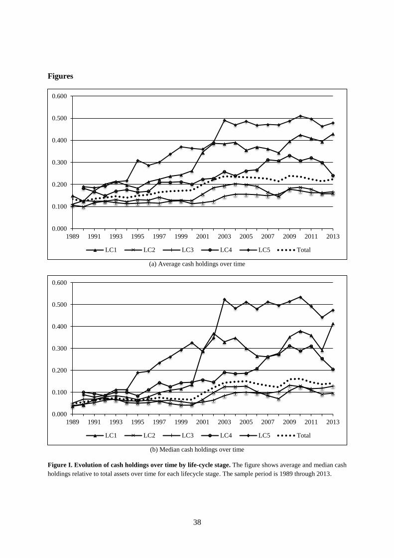
38
Figures
(a) Average cash holdings over time
(b) Median cash holdings over time
Figure I. Evolution of cash holdings over time by life-cycle stage. The figure shows average and median cash
holdings relative to total assets over time for each lifecycle stage. The sample period is 1989 through 2013.
0.000
0.100
0.200
0.300
0.400
0.500
0.600
1989 1991 1993 1995 1997 1999 2001 2003 2005 2007 2009 2011 2013
LC1 LC2 LC3 LC4 LC5 Total
0.000
0.100
0.200
0.300
0.400
0.500
0.600
1989 1991 1993 1995 1997 1999 2001 2003 2005 2007 2009 2011 2013
LC1 LC2 LC3 LC4 LC5 Total

39
(a) Proportions of firms per life-cycle stage over time (equal-weighted)
(b) Proportions of firms per life-cycle stage over time (value-weighted)
Figure II. Proportions of firms per life-cycle stage over time. The figure shows equal-weighted and value
weighted proportions of firms per lifecycle stage over time. The sample period is 1989 through 2013.
0.000
0.100
0.200
0.300
0.400
0.500
0.600
1989 1991 1993 1995 1997 1999 2001 2003 2005 2007 2009 2011 2013
LC1 LC2 LC3 LC4 LC5
0.000
0.100
0.200
0.300
0.400
0.500
0.600
0.700
0.800
1989 1991 1993 1995 1997 1999 2001 2003 2005 2007 2009 2011 2013
LC1 LC2 LC3 LC4 LC5