Corporate Greenhouse Gas Inventories for the Agricultural ... · Product Life Cycle Accounting and...
28
WORKING PAPER World resources InstItute • 10 G Street, NE • Washington, DC 20002 • Tel: 1-202-729-7600 • Fax: 1-202-729-7610 • www.wri.org World Resources Institute Working Papers contain preliminary research, analysis, findings, and recommendations. They are circulated to stimulate timely discussion and critical feedback and to influence ongoing debate on emerging issues. Most working papers are eventually published in another form and their content may be revised. Suggested citation: Russell, S. 2011. “Corporate Greenhouse Gas Inventories for the Agricultural Sector: Proposed accounting and reporting steps.” WRI Working Paper. World Resources Institute, Washington, DC. 29 pp. Available online at http://www.wri.org/ publications. January 2011 Corporate Greenhouse Gas Inventories for the Agricultural Sector: Proposed Accounting and Reporting Steps STEPHEN RUSSELL Contents Summary ................................ 1 About the GHG Protocol ...................... 2 1. Introduction ............................. 3 2. What Emission Sources Are Associated with Agriculture? ................. 5 3. Which Emission Sources Should Be Included in an Inventory? ................... 8 4. How Are GHG Data Calculated? ............. 14 5. How Should GHG Data Be Reported? ......... 20 Appendices .............................. 23 Glossary ................................ 27 References .............................. 29 Corporate inventories of greenhouse gas (GHG) emissions provide a firm foundation for emissions management by business. But they rarely include agricultural emissions, often because of confusion about the best practices needed to address unique aspects of agricultural sources. This paper suggests accounting and reporting procedures based on the GHG Protocol Corporate Accounting and Reporting Standard. The objective is to stimulate and inform discussion amongst stakeholders towards a common understanding of best practices. summary Agricultural activities cause greenhouse gas (GHG) emissions from a diverse range of sources. An equally diverse range of issues affects whether and how these emissions should be included in corporate GHG emissions inventories. This paper provides a preliminary assessment of these issues and how they can be addressed within the framework provided by the GHG Protocol Corporate Accounting and Reporting Standard (Corporate Standard). The key findings are: 1. The Corporate Standard outlines generic accounting procedures that are directly applicable to many of the organizational and operational structures common in the agricultural sector, such as co-operatives, leasing arrangements, and commodity production contracts. 2. Accounting for the GHG emissions from equipment and machinery on farms is relatively straightforward. But the emissions from non-mechani- cal sources, such as soils and livestock, are more challenging. Specific challenges include the variability in GHG emission rates over time and space, the difficulty in disentangling the effects of current management practices on GHG emissions from those caused by natural factors, and
-
Upload
phungduong -
Category
Documents
-
view
213 -
download
0
Transcript of Corporate Greenhouse Gas Inventories for the Agricultural ... · Product Life Cycle Accounting and...
W O R K I N G P A P E R
World resources InstItute • 10 G Street, NE • Washington, DC 20002 • Tel: 1-202-729-7600 • Fax: 1-202-729-7610 • www.wri.org
World Resources Institute Working Papers contain
preliminary research, analysis, findings, and
recommendations. They are circulated to stimulate timely
discussion and critical feedback and to influence ongoing
debate on emerging issues. Most working papers are
eventually published in another form and their content may
be revised.
Suggested citation: Russell, S. 2011. “Corporate Greenhouse Gas Inventories for the Agricultural Sector: Proposed accounting and reporting steps.” WRI Working Paper. World Resources Institute, Washington, DC. 29 pp. Available online at http://www.wri.org/publications.
January 2011
Corporate Greenhouse Gas Inventories for the Agricultural Sector: Proposed Accounting and Reporting Steps
STePhen RuSSell
ContentsSummary . . . . . . . . . . . . . . . . . . . . . . . . . . . . . . . . 1
About the GhG Protocol . . . . . . . . . . . . . . . . . . . . . . 2
1. Introduction . . . . . . . . . . . . . . . . . . . . . . . . . . . . . 3
2. What emission Sources Are Associated with Agriculture? . . . . . . . . . . . . . . . . . 5
3. Which emission Sources Should Be Included in an Inventory? . . . . . . . . . . . . . . . . . . . 8
4. how Are GhG Data Calculated? . . . . . . . . . . . . . 14
5. how Should GhG Data Be Reported? . . . . . . . . . 20
Appendices . . . . . . . . . . . . . . . . . . . . . . . . . . . . . . 23
Glossary . . . . . . . . . . . . . . . . . . . . . . . . . . . . . . . . 27
References . . . . . . . . . . . . . . . . . . . . . . . . . . . . . . 29
Corporate inventories of greenhouse gas (GHG) emissions provide a firm foundation for emissions management by business. But they rarely include agricultural emissions, often because of confusion about the best practices needed to address unique aspects of agricultural sources. This paper suggests accounting and reporting procedures based on the GHG Protocol Corporate Accounting and Reporting Standard. The objective is to stimulate and inform discussion amongst stakeholders towards a common understanding of best practices.
summaryAgricultural activities cause greenhouse gas (GHG) emissions from a diverse range of sources. An equally diverse range of issues affects whether and how these emissions should be included in corporate GHG emissions inventories. This paper provides a preliminary assessment of these issues and how they can be addressed within the framework provided by the GHG Protocol Corporate Accounting and Reporting Standard (Corporate Standard). The key findings are:
1. The Corporate Standard outlines generic accounting procedures that are directly applicable to many of the organizational and operational structures common in the agricultural sector, such as co-operatives, leasing arrangements, and commodity production contracts.
2. Accounting for the GHG emissions from equipment and machinery on farms is relatively straightforward. But the emissions from non-mechani-cal sources, such as soils and livestock, are more challenging. Specific challenges include the variability in GHG emission rates over time and space, the difficulty in disentangling the effects of current management practices on GHG emissions from those caused by natural factors, and
WORLD RESOURCES INSTITUTE | WORKING PAPER2
the reversibility of carbon stocks and the long timescales over which carbon stocks change.
3. Consensus best practices for dealing with these chal-lenges do not yet exist, but such best practices might include:
l Separately reporting GHG data on mechanical and non-mechanical sources within inventories
l Reporting carbon stock information using data on both stock size and carbon dioxide (CO2) fluxes
l Allocating long-term changes in carbon stocks evenly across multiple reporting periods
l Reporting the current impact of historical changes in land management practices on carbon stocks. Compa-nies should adopt a time threshold to determine when historical management changes are relevant
l Reporting all GHG emissions from land use change under an appropriate scope and not as a separate memo item.
This paper concentrates on core GHG accounting and reporting issues, but a range of other issues are also relevant to the creation of GHG inventories. For instance: What business goals do agricultural companies have for address-ing climate change and how are GHG inventories useful in meeting these goals? How can companies acquire the activity data needed to calculate GHG emissions? And what gaps exist in emissions calculation methodologies and how should these gaps be handled within GHG inventories?
The GHG Protocol intends to develop a consensus-based GHG accounting and reporting protocol for the sector. A crucial next step is to conduct broad stakeholder consulta-tions on this paper and identify remaining questions.
about the GhG ProtoColThe GHG Protocol is a decade-long partnership between the World Resources Institute and the World Business Council for Sustainable Development. It works with businesses, governments, and environmental groups around the world to build a new generation of credible and effec-tive standards for the accounting and reporting of GHG emissions at the corporate, project, and product levels.
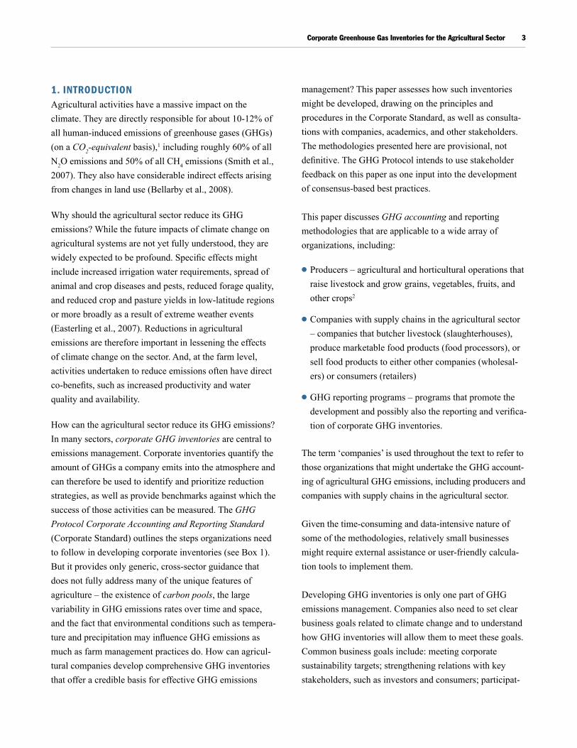
LEvEL OF GHG ANALySIS
Corporate Project Product
Applicable GhG Protocol standard or protocol
Corporate Accounting and Reporting Standard
Scope 3 Accounting and Reporting Standard
Protocol for Project Accounting
Product Life Cycle Accounting and Reporting Standard
What does the publication do?
Describes how emissions data from across the entire operations of companies can be consolidated into single inventories
Provides detailed directions on including the emissions from supply chain operations in corporate inventories
Describes how to measure the GhG benefits of projects undertaken to reduce emissions, avoid future emissions or sequester GhGs
Describes how the GhG impacts of products can be measured throughout the entire product life cycle
Other GhG Protocol publications relevant to the agricultural sector
The GHG Protocol for the Agricultural Sector: Interpreting the Corporate Standard for Agricultural Companies (under development and to be partially based on this Working Paper)
The Land Use, Land-Use Change, and Forestry Guidance for GHG Project Accounting
Corporate Greenhouse Gas Inventories for the Agricultural Sector 3
1. IntroduCtIonAgricultural activities have a massive impact on the climate. They are directly responsible for about 10-12% of all human-induced emissions of greenhouse gases (GHGs) (on a CO2-equivalent basis),1 including roughly 60% of all N2O emissions and 50% of all CH4 emissions (Smith et al., 2007). They also have considerable indirect effects arising from changes in land use (Bellarby et al., 2008).
Why should the agricultural sector reduce its GHG emissions? While the future impacts of climate change on agricultural systems are not yet fully understood, they are widely expected to be profound. Specific effects might include increased irrigation water requirements, spread of animal and crop diseases and pests, reduced forage quality, and reduced crop and pasture yields in low-latitude regions or more broadly as a result of extreme weather events (Easterling et al., 2007). Reductions in agricultural emissions are therefore important in lessening the effects of climate change on the sector. And, at the farm level, activities undertaken to reduce emissions often have direct co-benefits, such as increased productivity and water quality and availability.
How can the agricultural sector reduce its GHG emissions? In many sectors, corporate GHG inventories are central to emissions management. Corporate inventories quantify the amount of GHGs a company emits into the atmosphere and can therefore be used to identify and prioritize reduction strategies, as well as provide benchmarks against which the success of those activities can be measured. The GHG Protocol Corporate Accounting and Reporting Standard (Corporate Standard) outlines the steps organizations need to follow in developing corporate inventories (see Box 1). But it provides only generic, cross-sector guidance that does not fully address many of the unique features of agriculture – the existence of carbon pools, the large variability in GHG emissions rates over time and space, and the fact that environmental conditions such as tempera-ture and precipitation may influence GHG emissions as much as farm management practices do. How can agricul-tural companies develop comprehensive GHG inventories that offer a credible basis for effective GHG emissions
management? This paper assesses how such inventories might be developed, drawing on the principles and procedures in the Corporate Standard, as well as consulta-tions with companies, academics, and other stakeholders. The methodologies presented here are provisional, not definitive. The GHG Protocol intends to use stakeholder feedback on this paper as one input into the development of consensus-based best practices.
This paper discusses GHG accounting and reporting methodologies that are applicable to a wide array of organizations, including:
l Producers – agricultural and horticultural operations that raise livestock and grow grains, vegetables, fruits, and other crops2
l Companies with supply chains in the agricultural sector – companies that butcher livestock (slaughterhouses), produce marketable food products (food processors), or sell food products to either other companies (wholesal-ers) or consumers (retailers)
l GHG reporting programs – programs that promote the development and possibly also the reporting and verifica-tion of corporate GHG inventories.
The term ‘companies’ is used throughout the text to refer to those organizations that might undertake the GHG account-ing of agricultural GHG emissions, including producers and companies with supply chains in the agricultural sector.
Given the time-consuming and data-intensive nature of some of the methodologies, relatively small businesses might require external assistance or user-friendly calcula-tion tools to implement them.
Developing GHG inventories is only one part of GHG emissions management. Companies also need to set clear business goals related to climate change and to understand how GHG inventories will allow them to meet these goals. Common business goals include: meeting corporate sustainability targets; strengthening relations with key stakeholders, such as investors and consumers; participat-
WORLD RESOURCES INSTITUTE | WORKING PAPER4
ing in GHG reporting programs or the carbon market; and preparing for anticipated GHG regulations. While business goals can influence the design of GHG inventories (see Section 3.1 for an example), this paper does not attempt to characterize those goals specific to agricultural companies. The following issues are also not considered here:
l The sale of offset credits (see Box 2) or the use of on-site renewable energy that has been generated on farmland. The GHG Protocol is currently developing separate guid-ance on reflecting such trades in corporate GHG invento-ries.
l Including managed woodland in corporate inventories. While woodland is a common farm feature, accounting for changes in woodland carbon pools can entail quite different challenges from those encountered in account-ing for livestock and crop production, especially if wood products have been produced. Nonetheless, this paper
has some relevance to the management of farm wood-land since it proposes ways to account for the conversion of woodland (and other land-use categories) to arable land and vice versa.
l Accounting for the carbon dioxide (CO2) emissions from the combustion of biofuels. While the methane (CH4) and nitrous oxide (N2O) emissions from biofuel combus-tion should be reported in inventories, consensus on the accounting methodologies for CO2 emissions has not yet materialized and requires the analysis of complex life cycle accounting issues that are beyond the purview of the Corporate Standard.
l Choosing methodologies and tools for calculating GHG emissions. While obtaining accurate GHG emissions data often presents significant challenges to the develop-ment of agricultural GHG inventories, this paper does not provide guidance on selecting or using calculation
Box 1 | the GhG Protocol Corporate accounting and reporting standard
The GHG Protocol Corporate Accounting and Reporting
Standard (Corporate Standard)* was developed to:
• help companies prepare GhG emissions inventories that
are true and fair accounts of their climate impact
• Simplify and reduce the costs of compiling a GhG inventory
• enable GhG inventories to meet the decision-making needs
of both internal management and external stakeholders
(e.g., investors)
• Provide businesses with information that can be used to
build effective GhG management strategies
• Increase consistency and transparency in GhG accounting
and reporting among various companies and GhG programs.
The Corporate Standard is the leading international business
tool for developing corporate GhG inventories. It has been
adopted by virtually all mandatory and voluntary GhG
reporting programs around the world, such as the Carbon
Disclosure Project and The Climate Registry; by multiple,
industry-led sustainability initiatives, such as the Cement
Sustainability Initiative; and by the International Standards
Organization (ISO). Further examples of users of the
Corporate Standard can be found at: http://www.ghgproto-
col.org/standards/corporate-standard/users-of-the-corpo-
rate-standard.
* Revised edition. 2004. World Resources Institute and World Business Council for Sustainable Development. Available at: http://www.ghgprotocol.org/standards/corporate-standard.
Corporate Greenhouse Gas Inventories for the Agricultural Sector 5
methodologies, only on procedures for the accounting and reporting of emissions data. Section 5 briefly reviews different types of calculation methodologies as a context for these procedures.
l Methodologies for creating product-level GHG invento-ries (Box 3).
After reviewing the emission sources associated with agriculture (Section 2), this paper considers the main steps in developing corporate inventories in the order that they are practiced: accounting for emission sources (Section 3), calculating emissions (Section 4), and reporting emissions data (Section 5).
2. What emIssIon sourCes are assoCIated WIth aGrICulture? Agriculture causes emissions from a diverse range of sources, both on farmland and beyond the farm gate (Figure 1). The main GHGs involved are:
Box 2 | agriculture offset Projects
Project-level accounting involves the quantification of the
GhG effects of projects designed to reduce GhG emissions,
enhance carbon sequestration, or avoid future emissions.
These projects may generate offset credits that are then
purchased by third parties to compensate for the GhG
emissions occurring along their value chains. Soil carbon
sequestration offers most (~89%) of the global potential
for reducing the emissions from agriculture (Smith et al.,
2007), and is often considered an important potential
source of offset credits. The Corporate Standard does not
address the accounting steps needed to create offset
credits. For such guidance readers should instead refer to
two companion GhG Protocol publications: The GHG
Protocol for Project Accounting (Project Protocol) and Land
Use, Land-Use Change, and Forestry Guidance for GHG
Project Accounting. See http://www.ghgprotocol.org/
standards/project-protocol.
Box 3 | Product-level GhG Inventories
A product-level GhG inventory is a compilation and
evaluation of the inputs, outputs, and potential GhG
impacts of a product – whether it be a good or a service
– throughout its entire life cycle. The GhG Protocol is
developing a new standard, the GHG Protocol Product Life
Cycle Accounting and Reporting Standard (‘Product
Standard’), to aid the development of product life cycle
inventories for public disclosure. The Product Standard
aims to support various business objectives, such as
identifying emissions reduction opportunities along a
product’s supply chain, performance tracking, and product
differentiation.
Corporate (including scopes 1, 2, and 3) and product-level
GhG inventories account for the value chain or life cycle
impacts of a company’s products and both types of
inventories require collecting data from suppliers and other
companies in the value chain. Consequently, while distinct,
corporate and product-level GhG inventories are mutually
supportive. For instance, companies compiling corporate
inventories may use product-level GhG data to calculate the
upstream and downstream scope 3 emissions associated
with products. Conversely, before compiling product-level
inventories, companies may find it useful to account for their
scope 3 emissions in order to identify the individual product
categories that contribute most to total value chain
emissions. Theoretically, the sum of the life cycle emissions
of each of a company’s products should approximate the
sum of that company’s value chain emissions.
l Refrigerants such as perfluorocarbons (PFCs) and hydrofluorocarbons (HFCs) are also released in smaller quantities
l CO2
l CH4
l N2O
It is fundamentally important to distinguish between two categories of emission sources found on farms. Mechanical sources consume fuels or electricity and largely emit GHGs through the physical process of combustion, either at the site
WORLD RESOURCES INSTITUTE | WORKING PAPER6
of power generation or consumption. Their emissions generally depend on how much combustion has occurred. Examples of mechanical sources include harvesting or irrigation equipment. In contrast, non-mechanical sources largely emit GHGs through bio-chemical processes and their emissions generally depend on a wide array of environmen-tal conditions (Table 1). Examples of non-mechanical sources include soils and enteric fermentation. The differ-ences between mechanical and non-mechanical sources have important implications for the design of GHG inventories.
What are the largest emission sources on farms? At a global level, non-mechanical sources are more significant than mechanical sources (U.S. EPA, 2006a), with enteric fermen-tation (CH4) and soils (N2O) being the most significant sources (U.S. EPA, 2006b). The exact contribution of agriculture to global CO2 emissions is hard to quantify. This is because the biomass and soil carbon pools associated
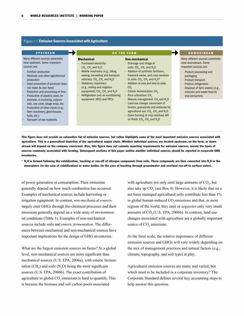
U p s t r e a m
Many different sources potentially exist upstream. Some important sources are:
• Fertilizer production • Pesticide and other agrichemical
production• Feed production (if producer does
not make its own feed)• extraction and processing of lime• Production of plastics used, for
example, in mulching, polytun-nels, row cover, silage wrap, etc.
• Production of other inputs (e.g., farm machinery, greenhouses, fuels, etc.)
• Transport of raw materials
Figure 1 | emission sources associated with agriculture
Mechanical• Purchased electricity:
CO2, Ch4 and n2O • Mobile machinery (e.g., tilling,
sowing, harvesting and transport vehicles): CO2, Ch4 and n2O
• Stationary machinery (e.g., milling and irrigation equipment): CO2, Ch4 and n2O
• Refrigeration and air-conditioning equipment: hFCs and PFCs
Non-mechanical• Drainage and tillage of
soils: CO2, Ch4 and n2O• Addition of synthetic fertilizers,
livestock waste, and crop residues to soils: CO2, Ch4 and n2O*
• Addition of urea and lime to soils: CO2
• enteric fermentation: Ch4
• Rice cultivation: Ch4
• Manure management: Ch4 and n2O
• Land use change: conversion of forests, grasslands and wetlands for agricultural use: CO2, Ch4 and n2O
• Open burning of crop residues left on fields: CO2, Ch4 and n2O
O n t h e f a r m
This figure does not provide an exhaustive list of emission sources, but rather highlights some of the most important emission sources associated with
agriculture. This is a generalized depiction of the agricultural supply chain. Whether individual sources are located upstream, on the farm, or down-
stream will depend on the company concerned. Also, this figure does not connote reporting requirements for emission sources, merely the types of
sources commonly associated with farming. Subsequent sections of this paper outline whether individual sources should be reported in corporate GHG
inventories.
* N2O is formed following the volatilization, leaching or run-off of nitrogen compounds from soils. These compounds are then converted into N2O in the
atmosphere (in the case of volatilization) or water bodies (in the case of leaching through groundwater and overland run-off to surface water).
D O w n s t r e a m
Many different sources potentially exist downstream. Some important sources are:
• Product processing and packaging
• Product transport• Product refrigeration • Disposal of farm wastes (e.g.,
manure) and waste food by end-consumers
with agriculture not only emit large amounts of CO2, but also take up CO2 (see Box 4). However, it is likely that on a net basis managed agricultural soils contribute less than 1% to global human-induced CO2 emissions and that, in most regions of the world, they emit or sequester only very small amounts of CO2 (U.S. EPA, 2006b). In contrast, land-use changes associated with agriculture are a globally important source of CO2 emissions.
At the farm scale, the relative importance of different emission sources and GHGs will vary widely depending on the mix of management practices and natural factors (e.g., climate, topography, and soil type) at play.
Agricultural emission sources are many and varied, but which need to be included in a corporate inventory? The Corporate Standard defines several key accounting steps to help answer this question.
Corporate Greenhouse Gas Inventories for the Agricultural Sector 7
Table 1 | How GHGs are Emitted by the Two Main Types of Sources on Farms
Type of source
GHG and process of emission
non- mechanical
Microbial processes:• CO2: from the microbial decay of organic matter (and, to a lesser extent, from the chemical oxidation of soil carbon)• Ch4: from the decomposition of organic materials in oxygen-deficient conditions (e.g., enteric fermentation, stored manures, flooded rice paddies)• n2O: from the microbial transformation of nitrogen in soils, manures, and water bodies
• CO2, Ch4, and n2O: from the combustion of biomass (e.g., crop residues, woodland, savannah)
• CO2: from the application of lime and urea to soils
Mechanical Fuel combustion:• CO2: from oxidation of carbon in fuels• Ch4 and n2O: emissions depend on combustion and emissions control technologies, age of vehicle, etc.
• hFCs and PFCs are also emitted by refrigeration and air-conditioning equipment
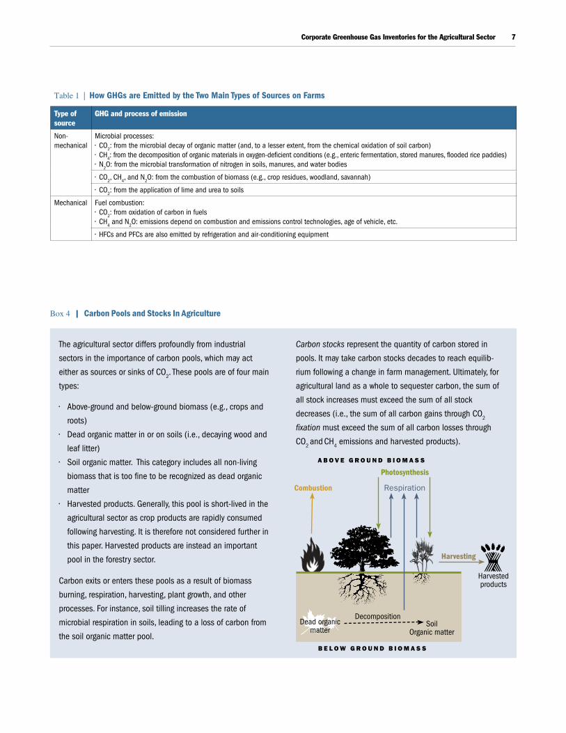
Box 4 | Carbon Pools and stocks In agriculture
The agricultural sector differs profoundly from industrial
sectors in the importance of carbon pools, which may act
either as sources or sinks of CO2. These pools are of four main
types:
• Above-ground and below-ground biomass (e.g., crops and
roots)
• Dead organic matter in or on soils (i.e., decaying wood and
leaf litter)
• Soil organic matter. This category includes all non-living
biomass that is too fine to be recognized as dead organic
matter
• harvested products. Generally, this pool is short-lived in the
agricultural sector as crop products are rapidly consumed
following harvesting. It is therefore not considered further in
this paper. harvested products are instead an important
pool in the forestry sector.
Carbon exits or enters these pools as a result of biomass
burning, respiration, harvesting, plant growth, and other
processes. For instance, soil tilling increases the rate of
microbial respiration in soils, leading to a loss of carbon from
the soil organic matter pool.
Carbon stocks represent the quantity of carbon stored in
pools. It may take carbon stocks decades to reach equilib-
rium following a change in farm management. ultimately, for
agricultural land as a whole to sequester carbon, the sum of
all stock increases must exceed the sum of all stock
decreases (i.e., the sum of all carbon gains through CO2
fixation must exceed the sum of all carbon losses through
CO2 and Ch4 emissions and harvested products).
Combustion
Decomposition
Photosynthesis
Harvesting
SoilOrganic matter
a b O v e g r O U n D b i O m a s s
b e l O w g r O U n D b i O m a s s
harvested products
Respiration
Dead organic matter
WORLD RESOURCES INSTITUTE | WORKING PAPER8
3. WhICh emIssIon sourCes should be InCluded In an Inventory? Companies must set so-called organizational and opera-tional boundaries to identify the business operations and sources, respectively, which should be included in an inventory. To allow emissions performance to be consis-tently tracked over time, these steps need to be conducted for both the current reporting period and a base period.
3.1 Set organizational boundaries Organizational boundaries determine which business operations should be included in an inventory. Three ‘consolidation’ approaches can be used to set organiza-tional boundaries (for more information, see Chapter 3 of the Corporate Standard):
1. Operational control. An entity accounts for 100% of the emissions from an operation over which it has the authority to introduce and implement its own operating policies.
2. Financial control. An entity accounts for 100% of the emissions from an operation over which it has the ability to direct financial and operating policies with a view to gaining economic benefits.
3. Equity-share approach. An entity accounts for the emissions from an operation according to its share of equity (or percentage of economic interest) in that operation.
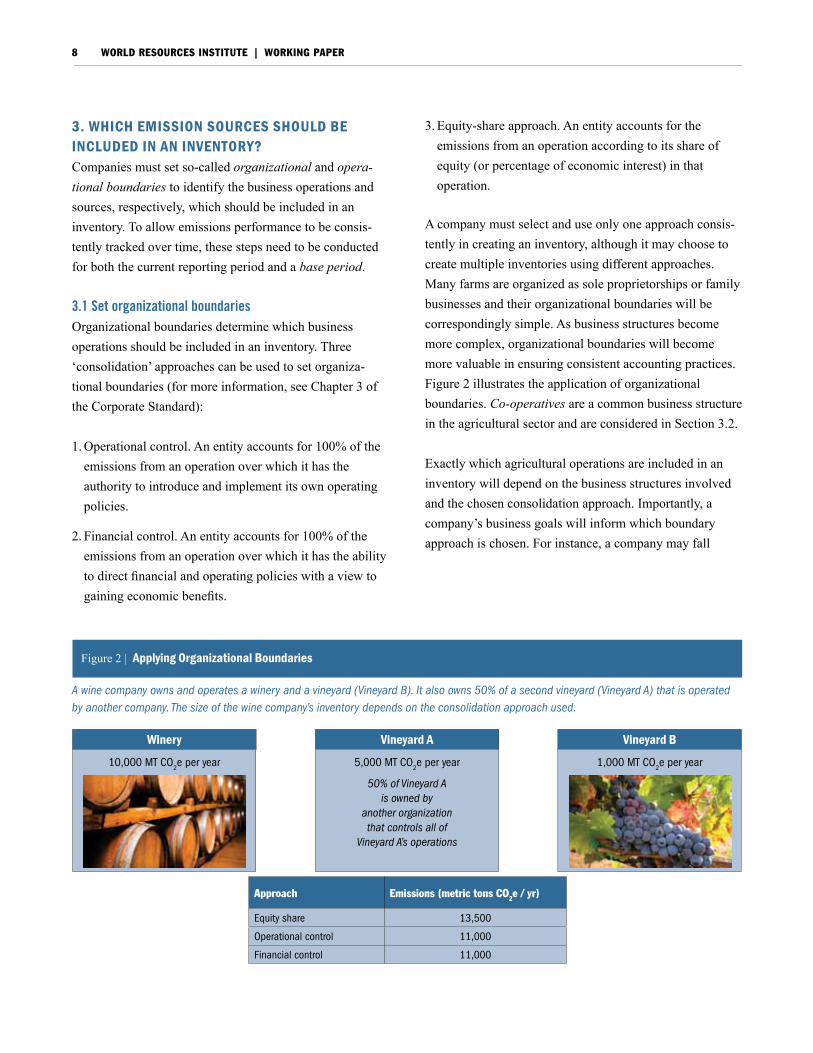
A company must select and use only one approach consis-tently in creating an inventory, although it may choose to create multiple inventories using different approaches. Many farms are organized as sole proprietorships or family businesses and their organizational boundaries will be correspondingly simple. As business structures become more complex, organizational boundaries will become more valuable in ensuring consistent accounting practices. Figure 2 illustrates the application of organizational boundaries. Co-operatives are a common business structure in the agricultural sector and are considered in Section 3.2.
Exactly which agricultural operations are included in an inventory will depend on the business structures involved and the chosen consolidation approach. Importantly, a company’s business goals will inform which boundary approach is chosen. For instance, a company may fall
Figure 2 | applying organizational boundaries
10,000 MT CO2e per year
Winery
Approach Emissions (metric tons CO2e / yr)
equity share 13,500
Operational control 11,000
Financial control 11,000
A wine company owns and operates a winery and a vineyard (Vineyard B). It also owns 50% of a second vineyard (Vineyard A) that is operated by another company. The size of the wine company’s inventory depends on the consolidation approach used.
vineyard a vineyard b
1,000 MT CO2e per year5,000 MT CO2e per year
50% of Vineyard A is owned by
another organization that controls all of
Vineyard A’s operations
Corporate Greenhouse Gas Inventories for the Agricultural Sector 9
under the jurisdiction of a cap-and-trade program and choose operational control, since compliance with the program would typically rest with the operators of emis-sion sources. Because this paper does not seek to identify business goals for developing GHG inventories, it does not consider which boundary approaches may be best suited to meeting these goals. The GHG Protocol intends to address these issues separately.
3.2 Set operational boundaries Having set organizational boundaries using any one of the consolidation approaches, companies should then set operational boundaries for each of their sources (for more information, see Chapter 4 of the Corporate Standard). These boundaries define whether an emission source is direct (i.e., is controlled or owned by the reporting entity) or indirect (i.e., the emissions are influenced by the reporting company, but the source itself is owned or controlled by a third party). Emission sources are further classified by scope:
l Scope 1: All direct sources
l Scope 2: Consumption of purchased electricity (an indirect source)
l Scope 3: All other indirect sources
Setting operational boundaries provides for the more effective management of GHG risks and opportunities along the supply chain and also minimizes the problem of double counting emissions. All scope 1 and 2 emissions should be reported in an inventory. Scope 3 emissions are reported optionally under the Corporate Standard, although it will be necessary to include many scope 3 sources in comprehensive analyses of supply chain emissions (see Section 5).
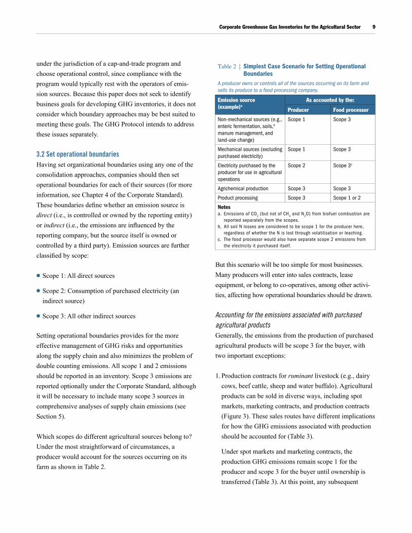
Which scopes do different agricultural sources belong to? Under the most straightforward of circumstances, a producer would account for the sources occurring on its farm as shown in Table 2.
But this scenario will be too simple for most businesses. Many producers will enter into sales contracts, lease equipment, or belong to co-operatives, among other activi-ties, affecting how operational boundaries should be drawn.
Accounting for the emissions associated with purchased agricultural products Generally, the emissions from the production of purchased agricultural products will be scope 3 for the buyer, with two important exceptions:
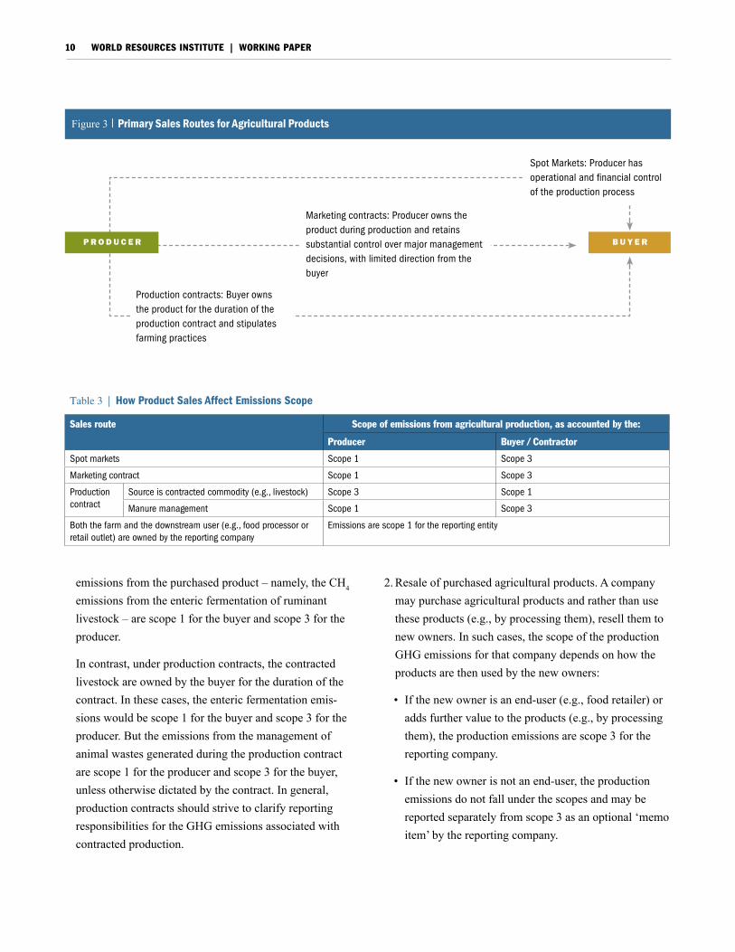
1. Production contracts for ruminant livestock (e.g., dairy cows, beef cattle, sheep and water buffalo). Agricultural products can be sold in diverse ways, including spot markets, marketing contracts, and production contracts (Figure 3). These sales routes have different implications for how the GHG emissions associated with production should be accounted for (Table 3).
Under spot markets and marketing contracts, the production GHG emissions remain scope 1 for the producer and scope 3 for the buyer until ownership is transferred (Table 3). At this point, any subsequent
Table 2 | Simplest Case Scenario for Setting Operational Boundaries
A producer owns or controls all of the sources occurring on its farm and sells its produce to a food processing company.
Emission source (example)a
As accounted by the:
Producer Food processor
non-mechanical sources (e.g., enteric fermentation, soils,b manure management, and land-use change)
Scope 1 Scope 3
Mechanical sources (excluding purchased electricity)
Scope 1 Scope 3
electricity purchased by the producer for use in agricultural operations
Scope 2 Scope 3c
Agrichemical production Scope 3 Scope 3
Product processing Scope 3 Scope 1 or 2
Notes a. emissions of CO2 (but not of Ch4 and n2O) from biofuel combustion are
reported separately from the scopes. b. All soil n losses are considered to be scope 1 for the producer here,
regardless of whether the n is lost through volatilization or leaching. c. The food processor would also have separate scope 2 emissions from
the electricity it purchased itself.
WORLD RESOURCES INSTITUTE | WORKING PAPER10
2. Resale of purchased agricultural products. A company may purchase agricultural products and rather than use these products (e.g., by processing them), resell them to new owners. In such cases, the scope of the production GHG emissions for that company depends on how the products are then used by the new owners:
• If the new owner is an end-user (e.g., food retailer) or adds further value to the products (e.g., by processing them), the production emissions are scope 3 for the reporting company.
• If the new owner is not an end-user, the production emissions do not fall under the scopes and may be reported separately from scope 3 as an optional ‘memo item’ by the reporting company.
emissions from the purchased product – namely, the CH4 emissions from the enteric fermentation of ruminant livestock – are scope 1 for the buyer and scope 3 for the producer.
In contrast, under production contracts, the contracted livestock are owned by the buyer for the duration of the contract. In these cases, the enteric fermentation emis-sions would be scope 1 for the buyer and scope 3 for the producer. But the emissions from the management of animal wastes generated during the production contract are scope 1 for the producer and scope 3 for the buyer, unless otherwise dictated by the contract. In general, production contracts should strive to clarify reporting responsibilities for the GHG emissions associated with contracted production.
p r O D U c e r b U y e r
Marketing contracts: Producer owns the product during production and retains substantial control over major management decisions, with limited direction from the buyer
Spot Markets: Producer has operational and financial control of the production process
Production contracts: Buyer owns the product for the duration of the production contract and stipulates farming practices
Figure 3 | Primary sales routes for agricultural Products
Table 3 | How Product Sales Affect Emissions Scope
Sales route Scope of emissions from agricultural production, as accounted by the:
Producer Buyer / Contractor
Spot markets Scope 1 Scope 3
Marketing contract Scope 1 Scope 3
Production contract
Source is contracted commodity (e.g., livestock) Scope 3 Scope 1
Manure management Scope 1 Scope 3
Both the farm and the downstream user (e.g., food processor or retail outlet) are owned by the reporting company
emissions are scope 1 for the reporting entity
Corporate Greenhouse Gas Inventories for the Agricultural Sector 11
For example, a company might purchase raw, bulk sugar from producers and then sell this sugar on to industrial consumers. In this case, the production GHG emissions are scope 3 for the company. Alternatively, the company may sell the sugar to other traders, and in this case the production GHG emissions are a memo item.
Land and equipment leasesThe Corporate Standard (Appendix F)3 distinguishes between two general types of leases:
l Capital (or financial) leases: This type of lease enables the lessee to operate an asset and also gives the lessee all the risks and rewards of owning the asset. In a capital lease the lessee has use of the asset over most of its useful life. Assets leased under a capital or financial lease are considered wholly-owned assets in financial accounting and are recorded as such on the balance sheet.
l Operational leases: This type of lease enables the lessee to operate an asset, such as a building or a vehicle, but does not give the lessee any of the risks or rewards of owning that asset. In an operating lease the lessee only has use of the asset for some of its useful life. Any lease that is not a capital or financial lease is an operating lease.
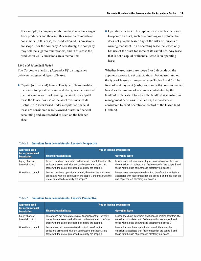
Whether leased assets are scope 1 or 3 depends on the approach chosen to set organizational boundaries and on the type of leasing arrangement (see Tables 4 and 5). The form of rent payment (cash, crops, or both) does not matter. Nor does the amount of resources contributed by the landlord or the extent to which the landlord is involved in management decisions. In all cases, the producer is considered to exert operational control of the leased land (Table 5).
Table 4 | Emissions from Leased Assets: Lessee’s Perspective
Approach used for organizational boundaries
Type of leasing arrangement
Financial/capital lease Operating lease
equity share or financial control
lessee does have ownership and financial control; therefore, the emissions associated with fuel combustion are scope 1 and those with the use of purchased electricity are scope 2
lessee does not have ownership or financial control; therefore, the emissions associated with fuel combustion are scope 3 and those with the use of purchased electricity are scope 3
Operational control lessee does have operational control; therefore, the emissions associated with fuel combustion are scope 1 and those with the use of purchased electricity are scope 2
lessee does have operational control; therefore, the emissions associated with fuel combustion are scope 1 and those with the use of purchased electricity are scope 2
Table 5 | Emissions from Leased Assets: Lessor’s Perspective
Approach used for organizational boundaries
Type of leasing arrangement
Financial/capital lease Operating lease
equity share or financial control
lessor does not have ownership or financial control; therefore, the emissions associated with fuel combustion are scope 3 and those with the use of purchased electricity are scope 3
lessor does have ownership and financial control; therefore, the emissions associated with fuel combustion are scope 1 and those with the use of purchased electricity are scope 2
Operational control lessor does not have operational control; therefore, the emissions associated with fuel combustion are scope 3 and those with the use of purchased electricity are scope 3
lessor does not have operational control; therefore, the emissions associated with fuel combustion are scope 3 and those with the use of purchased electricity are scope 3
WORLD RESOURCES INSTITUTE | WORKING PAPER12
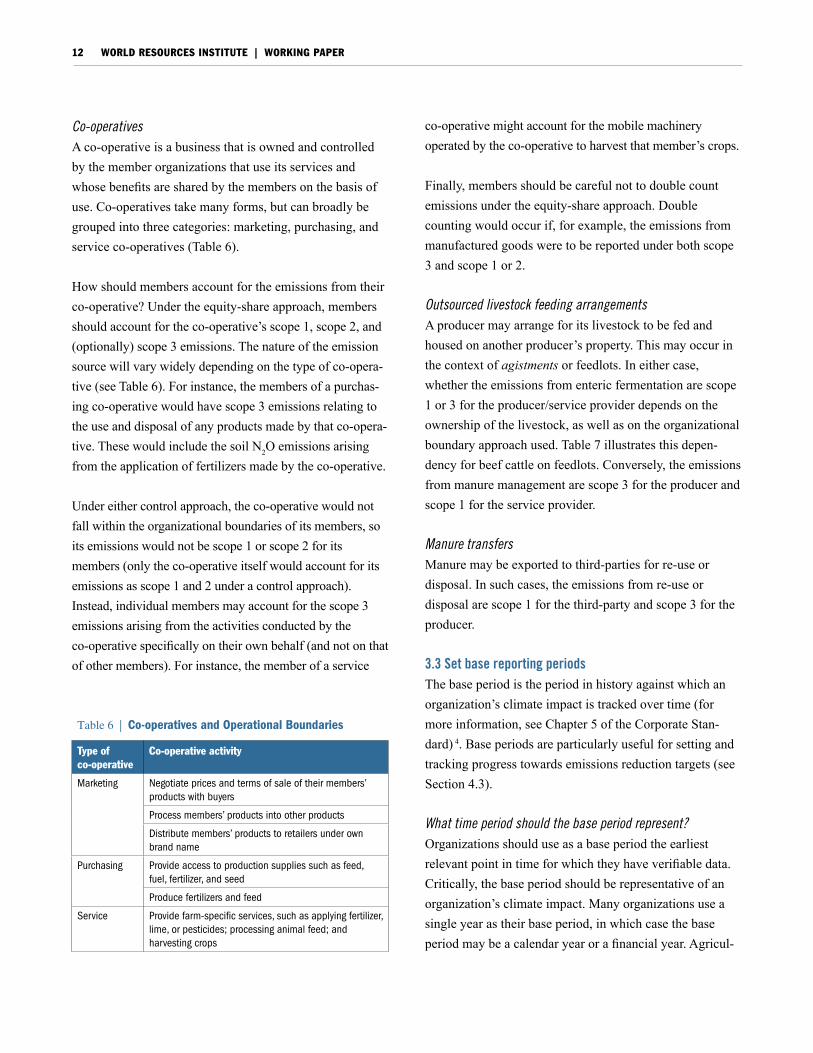
Co-operatives A co-operative is a business that is owned and controlled by the member organizations that use its services and whose benefits are shared by the members on the basis of use. Co-operatives take many forms, but can broadly be grouped into three categories: marketing, purchasing, and service co-operatives (Table 6).
How should members account for the emissions from their co-operative? Under the equity-share approach, members should account for the co-operative’s scope 1, scope 2, and (optionally) scope 3 emissions. The nature of the emission source will vary widely depending on the type of co-opera-tive (see Table 6). For instance, the members of a purchas-ing co-operative would have scope 3 emissions relating to the use and disposal of any products made by that co-opera-tive. These would include the soil N2O emissions arising from the application of fertilizers made by the co-operative.
Under either control approach, the co-operative would not fall within the organizational boundaries of its members, so its emissions would not be scope 1 or scope 2 for its members (only the co-operative itself would account for its emissions as scope 1 and 2 under a control approach). Instead, individual members may account for the scope 3 emissions arising from the activities conducted by the co-operative specifically on their own behalf (and not on that of other members). For instance, the member of a service
co-operative might account for the mobile machinery operated by the co-operative to harvest that member’s crops.
Finally, members should be careful not to double count emissions under the equity-share approach. Double counting would occur if, for example, the emissions from manufactured goods were to be reported under both scope 3 and scope 1 or 2.
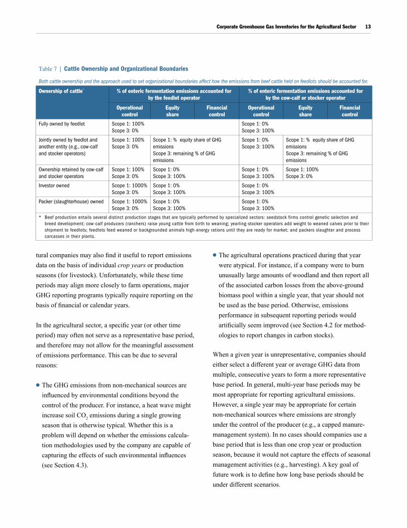
Outsourced livestock feeding arrangementsA producer may arrange for its livestock to be fed and housed on another producer’s property. This may occur in the context of agistments or feedlots. In either case, whether the emissions from enteric fermentation are scope 1 or 3 for the producer/service provider depends on the ownership of the livestock, as well as on the organizational boundary approach used. Table 7 illustrates this depen-dency for beef cattle on feedlots. Conversely, the emissions from manure management are scope 3 for the producer and scope 1 for the service provider.
Manure transfersManure may be exported to third-parties for re-use or disposal. In such cases, the emissions from re-use or disposal are scope 1 for the third-party and scope 3 for the producer.
3.3 Set base reporting periodsThe base period is the period in history against which an organization’s climate impact is tracked over time (for more information, see Chapter 5 of the Corporate Stan-dard) 4. Base periods are particularly useful for setting and tracking progress towards emissions reduction targets (see Section 4.3).
What time period should the base period represent?Organizations should use as a base period the earliest relevant point in time for which they have verifiable data. Critically, the base period should be representative of an organization’s climate impact. Many organizations use a single year as their base period, in which case the base period may be a calendar year or a financial year. Agricul-
Table 6 | Co-operatives and Operational Boundaries
Type of co-operative
Co-operative activity
Marketing negotiate prices and terms of sale of their members’ products with buyers
Process members’ products into other products
Distribute members’ products to retailers under own brand name
Purchasing Provide access to production supplies such as feed, fuel, fertilizer, and seed
Produce fertilizers and feed
Service Provide farm-specific services, such as applying fertilizer, lime, or pesticides; processing animal feed; and harvesting crops
Corporate Greenhouse Gas Inventories for the Agricultural Sector 13
tural companies may also find it useful to report emissions data on the basis of individual crop years or production seasons (for livestock). Unfortunately, while these time periods may align more closely to farm operations, major GHG reporting programs typically require reporting on the basis of financial or calendar years.
In the agricultural sector, a specific year (or other time period) may often not serve as a representative base period, and therefore may not allow for the meaningful assessment of emissions performance. This can be due to several reasons:
l The GHG emissions from non-mechanical sources are influenced by environmental conditions beyond the control of the producer. For instance, a heat wave might increase soil CO2 emissions during a single growing season that is otherwise typical. Whether this is a problem will depend on whether the emissions calcula-tion methodologies used by the company are capable of capturing the effects of such environmental influences (see Section 4.3).
l The agricultural operations practiced during that year were atypical. For instance, if a company were to burn unusually large amounts of woodland and then report all of the associated carbon losses from the above-ground biomass pool within a single year, that year should not be used as the base period. Otherwise, emissions performance in subsequent reporting periods would artificially seem improved (see Section 4.2 for method-ologies to report changes in carbon stocks).
When a given year is unrepresentative, companies should either select a different year or average GHG data from multiple, consecutive years to form a more representative base period. In general, multi-year base periods may be most appropriate for reporting agricultural emissions. However, a single year may be appropriate for certain non-mechanical sources where emissions are strongly under the control of the producer (e.g., a capped manure-management system). In no cases should companies use a base period that is less than one crop year or production season, because it would not capture the effects of seasonal management activities (e.g., harvesting). A key goal of future work is to define how long base periods should be under different scenarios.
Table 7 | Cattle Ownership and Organizational Boundaries
Both cattle ownership and the approach used to set organizational boundaries affect how the emissions from beef cattle held on feedlots should be accounted for.
Ownership of cattle* % of enteric fermentation emissions accounted for by the feedlot operator
% of enteric fermentation emissions accounted for by the cow-calf or stocker operator
Operational control
Equity share
Financial control
Operational control
Equity share
Financial control
Fully owned by feedlot Scope 1: 100%Scope 3: 0%
Scope 1: 0%Scope 3: 100%
Jointly owned by feedlot and another entity (e.g., cow-calf and stocker operators)
Scope 1: 100%Scope 3: 0%
Scope 1: % equity share of GhG emissionsScope 3: remaining % of GhG emissions
Scope 1: 0%Scope 3: 100%
Scope 1: % equity share of GhG emissionsScope 3: remaining % of GhG emissions
Ownership retained by cow-calf and stocker operators
Scope 1: 100%Scope 3: 0%
Scope 1: 0%Scope 3: 100%
Scope 1: 0%Scope 3: 100%
Scope 1: 100%Scope 3: 0%
Investor owned Scope 1: 1000%Scope 3: 0%
Scope 1: 0%Scope 3: 100%
Scope 1: 0%Scope 3: 100%
Packer (slaughterhouse) owned Scope 1: 1000%Scope 3: 0%
Scope 1: 0%Scope 3: 100%
Scope 1: 0%Scope 3: 100%
* Beef production entails several distinct production stages that are typically performed by specialized sectors: seedstock firms control genetic selection and breed development; cow-calf producers (ranchers) raise young cattle from birth to weaning; yearling-stocker operators add weight to weaned calves prior to their shipment to feedlots; feedlots feed weaned or backgrounded animals high-energy rations until they are ready for market; and packers slaughter and process carcasses in their plants.
WORLD RESOURCES INSTITUTE | WORKING PAPER14
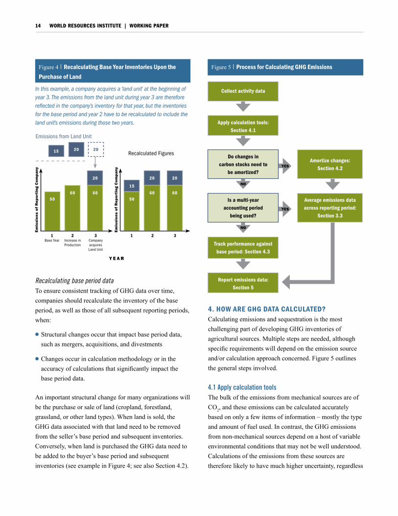
Recalculating base period dataTo ensure consistent tracking of GHG data over time, companies should recalculate the inventory of the base period, as well as those of all subsequent reporting periods, when:
l Structural changes occur that impact base period data, such as mergers, acquisitions, and divestments
l Changes occur in calculation methodology or in the accuracy of calculations that significantly impact the base period data.
An important structural change for many organizations will be the purchase or sale of land (cropland, forestland, grassland, or other land types). When land is sold, the GHG data associated with that land need to be removed from the seller’s base period and subsequent inventories. Conversely, when land is purchased the GHG data need to be added to the buyer’s base period and subsequent inventories (see example in Figure 4; see also Section 4.2).
4. hoW are GhG data CalCulated?Calculating emissions and sequestration is the most challenging part of developing GHG inventories of agricultural sources. Multiple steps are needed, although specific requirements will depend on the emission source and/or calculation approach concerned. Figure 5 outlines the general steps involved.
4.1 Apply calculation toolsThe bulk of the emissions from mechanical sources are of CO2, and these emissions can be calculated accurately based on only a few items of information – mostly the type and amount of fuel used. In contrast, the GHG emissions from non-mechanical sources depend on a host of variable environmental conditions that may not be well understood. Calculations of the emissions from these sources are therefore likely to have much higher uncertainty, regardless
Collect activity data
Apply calculation tools: Section 4.1
Report emissions data: Section 5
Do changes in carbon stocks need to
be amortized?
Amortize changes: Section 4.2
Is a multi-year accounting period
being used?
Average emissions data across reporting period:
Section 3.3
Track performance against base period: Section 4.3
Figure 5 | Process for Calculating GhG emissions
nO
nO
yes
yes
Recalculated Figures
emissions from land unit
em
issi
on
s o
f r
ep
ort
ing
co
mp
any
5060 60
20
2015 20
1Base Year
2 Increase in Production
3 Company acquires land unit
y e a r
em
issi
on
s o
f r
ep
ort
ing
co
mp
any
5060 60
2020
15
1 2 3
Figure 4 | recalculating base year Inventories upon the Purchase of land
In this example, a company acquires a ‘land unit’ at the beginning of year 3. The emissions from the land unit during year 3 are therefore reflected in the company’s inventory for that year, but the inventories for the base period and year 2 have to be recalculated to include the land unit’s emissions during those two years.
Corporate Greenhouse Gas Inventories for the Agricultural Sector 15
of the calculation approach chosen, and this affects how these sources should be reported (see Sections 4.3 and 5). Broadly, four different types of calculation approaches can be used for non-mechanical sources (Table 8).
Calculation tools and methodologies for both mechanical and non-mechanical sources are available from a number of providers, including corporate GHG reporting programs (e.g., U.S. Department of Energy 1605(b)),5 the Intergov-ernmental Panel on Climate Change (IPCC),6 and national inventory programs.7 The IPCC has defined different tiers of methodologies, which differ in terms of their method-ological complexity and data requirements:
l Tier 1: Simple, emission factor-based approach, where emissions are calculated by multiplying activity data by an appropriate emission factor. Tier 1 emission factors are international or regional defaults.
t i m er
at
es
Of
ch
an
ge
(to
nnes
CO
2/ye
ar)
6
4
2
0
—— CO2 fixation—— CO2 emissions
net decline in carbon stock
net increase in carbon stock
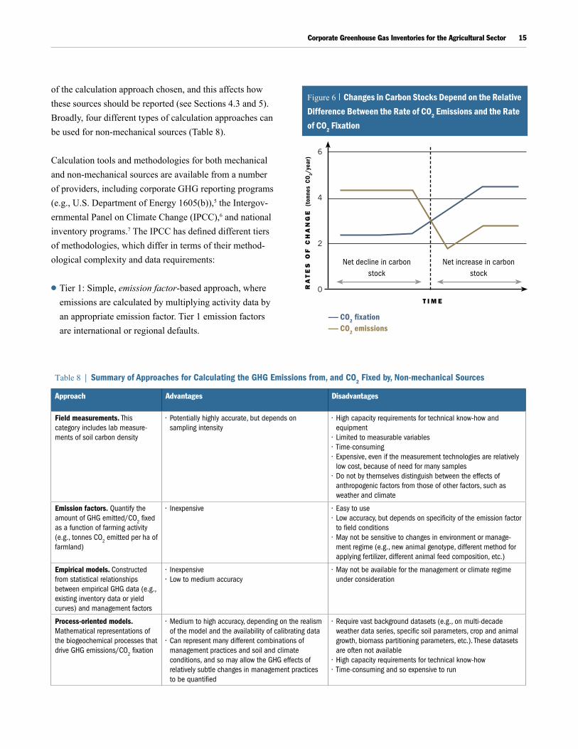
Figure 6 | Changes in Carbon stocks depend on the relative difference between the rate of Co2 emissions and the rate of Co2 Fixation
Table 8 | Summary of Approaches for Calculating the GHG Emissions from, and CO2 Fixed by, Non-mechanical Sources
Approach Advantages Disadvantages
Field measurements. This category includes lab measure-ments of soil carbon density
• Potentially highly accurate, but depends on sampling intensity
• high capacity requirements for technical know-how and equipment
• limited to measurable variables• Time-consuming• expensive, even if the measurement technologies are relatively
low cost, because of need for many samples• Do not by themselves distinguish between the effects of
anthropogenic factors from those of other factors, such as weather and climate
Emission factors. Quantify the amount of GhG emitted/CO
2 fixed as a function of farming activity (e.g., tonnes CO2 emitted per ha of farmland)
• Inexpensive • easy to use• low accuracy, but depends on specificity of the emission factor
to field conditions• May not be sensitive to changes in environment or manage-
ment regime (e.g., new animal genotype, different method for applying fertilizer, different animal feed composition, etc.)
Empirical models. Constructed from statistical relationships between empirical GhG data (e.g., existing inventory data or yield curves) and management factors
• Inexpensive• low to medium accuracy
• May not be available for the management or climate regime under consideration
Process-oriented models. Mathematical representations of the biogeochemical processes that drive GhG emissions/CO
2 fixation
• Medium to high accuracy, depending on the realism of the model and the availability of calibrating data
• Can represent many different combinations of management practices and soil and climate conditions, and so may allow the GhG effects of relatively subtle changes in management practices to be quantified
• Require vast background datasets (e.g., on multi-decade weather data series, specific soil parameters, crop and animal growth, biomass partitioning parameters, etc.). These datasets are often not available
• high capacity requirements for technical know-how• Time-consuming and so expensive to run
WORLD RESOURCES INSTITUTE | WORKING PAPER16
l Tier 2: More specific emission factors or more refined empirical estimation methodologies.
l Tier 3: Dynamic bio-geophysical simulation models using multi-year time series and context-specific parameterization.
Higher tier methodologies are considered more accurate (sensitive to changes in management) but are much more data-intensive. Cost, technical capacity, and desired accuracy, among other considerations, will influence which approach is most suited to meeting a business’s goals.
When calculating livestock emissions it is important to keep track of the amount of time that livestock has actually spent on the farm. For instance, lambs may only be on a farm for several months before they are sold to another company. In this case, the producer should be careful not to assume in its calculations that the livestock were on the farm for the full year.
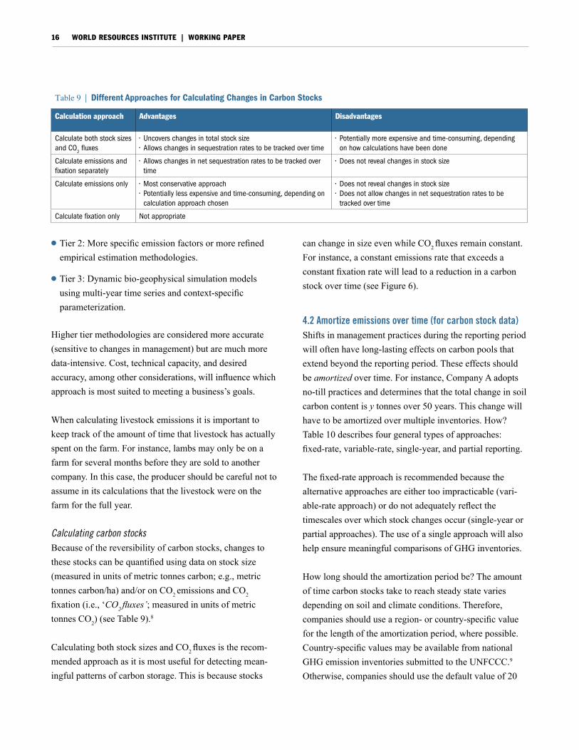
Calculating carbon stocksBecause of the reversibility of carbon stocks, changes to these stocks can be quantified using data on stock size (measured in units of metric tonnes carbon; e.g., metric tonnes carbon/ha) and/or on CO2 emissions and CO2
fixation (i.e., ‘CO2 fluxes’; measured in units of metric tonnes CO2) (see Table 9).8
Calculating both stock sizes and CO2 fluxes is the recom-mended approach as it is most useful for detecting mean-ingful patterns of carbon storage. This is because stocks
can change in size even while CO2 fluxes remain constant. For instance, a constant emissions rate that exceeds a constant fixation rate will lead to a reduction in a carbon stock over time (see Figure 6).
4.2 Amortize emissions over time (for carbon stock data)Shifts in management practices during the reporting period will often have long-lasting effects on carbon pools that extend beyond the reporting period. These effects should be amortized over time. For instance, Company A adopts no-till practices and determines that the total change in soil carbon content is y tonnes over 50 years. This change will have to be amortized over multiple inventories. How? Table 10 describes four general types of approaches: fixed-rate, variable-rate, single-year, and partial reporting.
The fixed-rate approach is recommended because the alternative approaches are either too impracticable (vari-able-rate approach) or do not adequately reflect the timescales over which stock changes occur (single-year or partial approaches). The use of a single approach will also help ensure meaningful comparisons of GHG inventories.
How long should the amortization period be? The amount of time carbon stocks take to reach steady state varies depending on soil and climate conditions. Therefore, companies should use a region- or country-specific value for the length of the amortization period, where possible. Country-specific values may be available from national GHG emission inventories submitted to the UNFCCC.9 Otherwise, companies should use the default value of 20
Table 9 | Different Approaches for Calculating Changes in Carbon Stocks
Calculation approach Advantages Disadvantages
Calculate both stock sizes and CO
2 fluxes• uncovers changes in total stock size• Allows changes in sequestration rates to be tracked over time
• Potentially more expensive and time-consuming, depending on how calculations have been done
Calculate emissions and fixation separately
• Allows changes in net sequestration rates to be tracked over time
• Does not reveal changes in stock size
Calculate emissions only • Most conservative approach• Potentially less expensive and time-consuming, depending on
calculation approach chosen
• Does not reveal changes in stock size• Does not allow changes in net sequestration rates to be
tracked over time
Calculate fixation only not appropriate
Corporate Greenhouse Gas Inventories for the Agricultural Sector 17
years for amortizing carbon stocks in national inventories (IPCC, 2006, Volume 4). Appendix II illustrates the use of a 20-year amortization period.
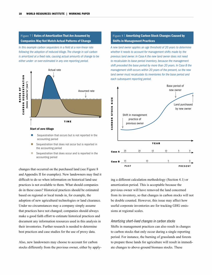
A central issue is that rates of soil CO2 fluxes are never constant. For instance, following the adoption of zero-tillage, the sequestration rate may initially be zero (or even negative), before reaching a maximum and then declining to zero (i.e., steady state; see Figure 7). In many cases, therefore, the (fixed) rate of amortization chosen by a company may not match actual patterns, and a given period’s inventory may under- or over-estimate the actual amount of change. As a result, companies need to carefully document the assumptions they have made in amortizing changes (see Section 5).
Amortizing carbon data from historical changes in land use or managementBecause stocks can take years to reach steady state, companies may have to account not only for management shifts that occur in the present, but also for those that occurred in the past. However, the older the shift in land management, the less likely it is to influence carbon stocks today. So, how far back in time do companies need to go? Companies should adopt an age threshold (x years) that is the same as the amortization period (e.g., x is 20 years if the default IPCC amortization period is used). If the shift happened within the x years preceding the base period or any subsequent reporting periods, then it needs to be reflected in the inventories for those periods.
Land transfers and amortizing carbon stocks
The purchase or sale of land triggers base period recalcula-tions (Section 3.3). In conducting these recalculations, new landowners should assess the need to amortize any stock
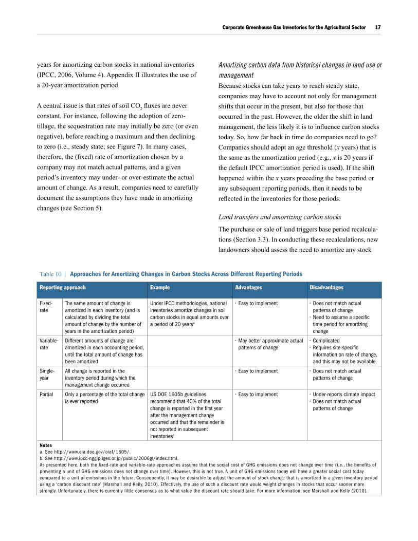
Table 10 | Approaches for Amortizing Changes in Carbon Stocks Across Different Reporting Periods
Reporting approach Example Advantages Disadvantages
Fixed-rate
The same amount of change is amortized in each inventory (and is calculated by dividing the total amount of change by the number of years in the amortization period)
under IPCC methodologies, national inventories amortize changes in soil carbon stocks in equal amounts over a period of 20 yearsa
• easy to implement • Does not match actual patterns of change
• need to assume a specific time period for amortizing change
Variable-rate
Different amounts of change are amortized in each accounting period, until the total amount of change has been amortized
• May better approximate actual patterns of change
• Complicated• Requires site-specific
information on rate of change, and this may not be available.
Single-year
All change is reported in the inventory period during which the management change occurred
• easy to implement • Does not match actual patterns of change
Partial Only a percentage of the total change is ever reported
uS DOe 1605b guidelines recommend that 40% of the total change is reported in the first year after the management change occurred and that the remainder is not reported in subsequent inventoriesb
• easy to implement • under-reports climate impact • Does not match actual
patterns of change
Notesa. See http://www.eia.doe.gov/oiaf/1605/.b. See http://www.ipcc-nggip.iges.or.jp/public/2006gl/index.html.As presented here, both the fixed-rate and variable-rate approaches assume that the social cost of GhG emissions does not change over time (i.e., the benefits of preventing a unit of GhG emissions does not change over time). however, this is not true. A unit of GhG emissions today will have a greater social cost today compared to a unit of emissions in the future. Consequently, it may be desirable to adjust the amount of stock change that is amortized in a given inventory period using a ‘carbon discount rate’ (Marshall and Kelly, 2010). effectively, the use of such a discount rate would weight changes in stocks that occur sooner more strongly. unfortunately, there is currently little consensus as to what value the discount rate should take. For more information, see Marshall and Kelly (2010).
WORLD RESOURCES INSTITUTE | WORKING PAPER18
changes that occurred on the purchased land (see Figure 8 and Appendix II for examples). New landowners may find it difficult to do so when information on historical land-use practices is not available to them. What should companies do in these cases? Historical practices should be estimated based on regional or local trends in, for example, the adoption of new agricultural technologies or land clearance. Under no circumstances may a company simply assume that practices have not changed; companies should always make a good faith effort to estimate historical practices and document any information resources used in this analysis in their inventories. Further research is needed to determine best practices and case studies for the use of proxy data.
Also, new landowners may choose to account for carbon stocks differently from the previous owner, either by apply-
ing a different calculation methodology (Section 4.1) or amortization period. This is acceptable because the previous owner will have removed the land concerned from its inventory, so that changes in carbon stocks will not be double counted. However, this issue may affect how useful corporate inventories are for tracking GHG emis-sions at regional scales.
Amortizing short-lived changes in carbon stocksShifts in management practices can also result in changes to carbon stocks that only occur during a single reporting period. For instance, the burning of grasslands and forests to prepare those lands for agriculture will result in immedi-ate changes to above-ground biomass stocks. These
P A S T P R E S E N T
case a
case b
Base period of new owner
Shift in management practice of
previous owner
land purchased by new owner
y e a r
ca
rb
On
st
Oc
k s
ize
Figure 8 | amortizing Carbon stock Changes Caused by shifts in management Practices
A new land owner applies an age threshold of 20 years to determine whether it needs to account for management shifts made by the previous land owner. In Case A the new land owner does not need to recalculate its base period inventory, because the management shift preceded the base period by more than 20 years. In Case B the management shift occurs within 20 years of the present, so the new land owner must recalculate its inventories for the base period and each subsequent reporting period.
n Sequestration that occurs but is not reported in the accounting period
n Sequestration that does not occur but is reported in the accounting period
n Sequestration that does occur and is reported in the accounting period
t i m e
ra
te
s O
f
ca
rb
On
se
qU
es
tr
at
iOn
(t
onne
s car
bon
ha-1/y
ear-1
)
Start of zero tillage
Actual rate
Assumed rate
Figure 7 | rates of amortization that are assumed by Companies may not match actual Patterns of Change
In this example carbon sequesters in a field at a non-linear rate following the adoption of reduced-tillage. The change in soil carbon is amortized at a fixed rate, causing actual amounts of change to be either under- or over-estimated in any one reporting period.
Corporate Greenhouse Gas Inventories for the Agricultural Sector 19
changes may either be reported during the reporting period in which they occurred or they may be amortized over time (Table 11). However, if a company purchases land that underwent such a shift within the chosen age threshold, it should amortize the carbon stock changes.
4.3 Track performance over time Historical management practices are not the only instance where factors other than ongoing farm management affect current emissions. For example:
l Natural variation in temperature and precipitation can affect soil N2O emissions.
l Indirect man-made factors, such as nitrogen deposition, air pollution, and CO2 fertilization, can alter patterns of carbon sequestration and soil N2O emissions.
This issue is important because inventories are only useful for managing emissions as long as they allow companies to track the effects of changes in management practices. However, the practical import of this issue depends on how emissions have been calculated. Many calculation method-ologies (e.g., Tier 1 IPCC methodologies) do not capture the effects of climate or indirect factors on GHG emissions. Instead, they only pick up changes in activity data (e.g.,
number of hectares farmed, number of cattle raised, amount of fertilizer used, etc.). In such cases, the calcu-lated GHG data only reflect management regimes and can be automatically used as a basis for emissions manage-ment. (Caveat: Many calculation methodologies may not be sensitive to changes in management practices and so may not allow changes in performance to be comprehen-sively tracked over time.)
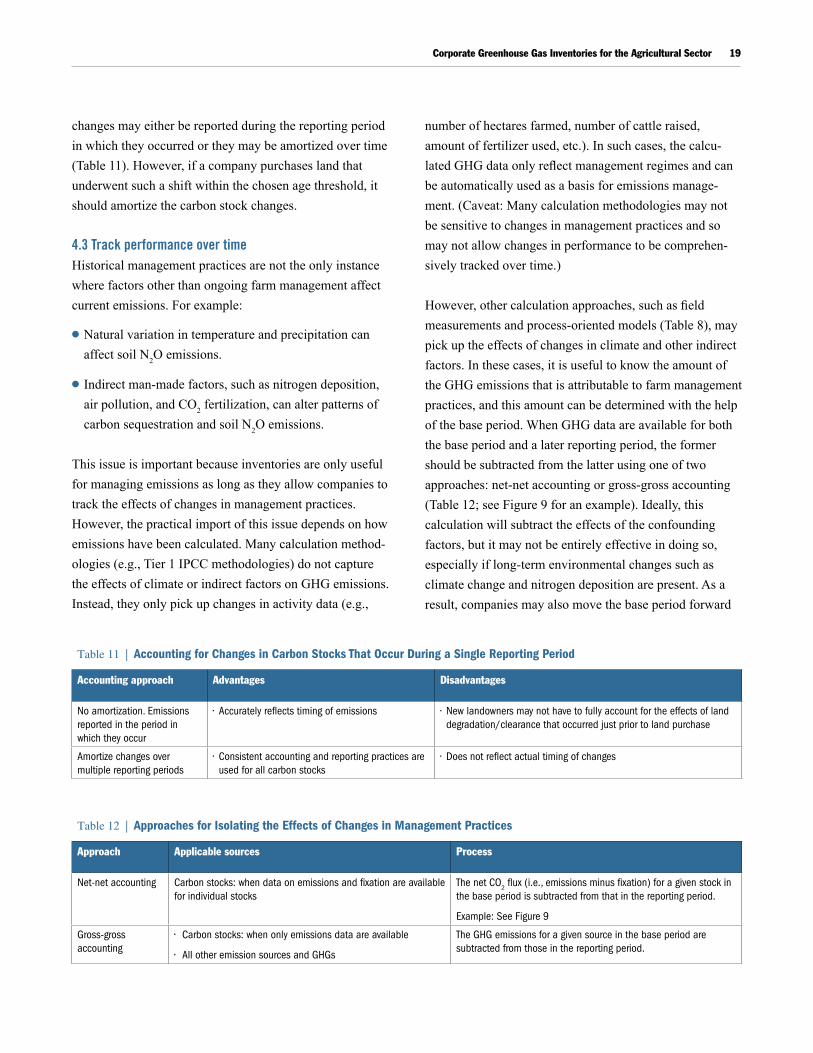
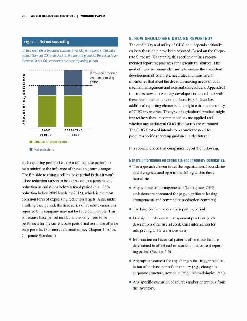
However, other calculation approaches, such as field measurements and process-oriented models (Table 8), may pick up the effects of changes in climate and other indirect factors. In these cases, it is useful to know the amount of the GHG emissions that is attributable to farm management practices, and this amount can be determined with the help of the base period. When GHG data are available for both the base period and a later reporting period, the former should be subtracted from the latter using one of two approaches: net-net accounting or gross-gross accounting (Table 12; see Figure 9 for an example). Ideally, this calculation will subtract the effects of the confounding factors, but it may not be entirely effective in doing so, especially if long-term environmental changes such as climate change and nitrogen deposition are present. As a result, companies may also move the base period forward
Table 11 | Accounting for Changes in Carbon Stocks That Occur During a Single Reporting Period
Accounting approach Advantages Disadvantages
no amortization. emissions reported in the period in which they occur
• Accurately reflects timing of emissions • new landowners may not have to fully account for the effects of land degradation/clearance that occurred just prior to land purchase
Amortize changes over multiple reporting periods
• Consistent accounting and reporting practices are used for all carbon stocks
• Does not reflect actual timing of changes
Table 12 | Approaches for Isolating the Effects of Changes in Management Practices
Approach Applicable sources Process
net-net accounting Carbon stocks: when data on emissions and fixation are available for individual stocks
The net CO2 flux (i.e., emissions minus fixation) for a given stock in
the base period is subtracted from that in the reporting period.
example: See Figure 9
Gross-gross accounting
• Carbon stocks: when only emissions data are available
• All other emission sources and GhGs
The GhG emissions for a given source in the base period are subtracted from those in the reporting period.
WORLD RESOURCES INSTITUTE | WORKING PAPER20
each reporting period (i.e., use a rolling base period) to help minimize the influence of these long-term changes. The flip side to using a rolling base period is that it won’t allow reduction targets to be expressed as a percentage reduction in emissions below a fixed period (e.g., 25% reduction below 2005 levels by 2015), which is the most common form of expressing reduction targets. Also, under a rolling base period, the time series of absolute emissions reported by a company may not be fully comparable. This is because base period recalculations only need to be performed for the current base period and not those of prior base periods. (For more information, see Chapter 11 of the Corporate Standard.)
5. hoW should GhG data be rePorted?The credibility and utility of GHG data depends critically on how those data have been reported. Based on the Corpo-rate Standard (Chapter 9), this section outlines recom-mended reporting practices for agricultural sources. The goal of these recommendations is to ensure the consistent development of complete, accurate, and transparent inventories that meet the decision-making needs of both internal management and external stakeholders. Appendix I illustrates how an inventory developed in accordance with these recommendations might look. Box 5 describes additional reporting elements that might enhance the utility of GHG inventories. The type of agricultural product might impact how these recommendations are applied and whether any additional GHG disclosures are warranted. The GHG Protocol intends to research the need for product-specific reporting guidance in the future.
It is recommended that companies report the following:
General information on corporate and inventory boundaries:l The approach chosen to set the organizational boundaries
and the agricultural operations falling within those boundaries
l Any contractual arrangements affecting how GHG emissions are accounted for (e.g., significant leasing arrangements and commodity production contracts)
l The base period and current reporting period
l Description of current management practices (such descriptions offer useful contextual information for interpreting GHG emissions data)
l Information on historical patterns of land use that are determined to affect carbon stocks in the current report-ing period (Section 3.3)
l Appropriate context for any changes that trigger recalcu-lation of the base period’s inventory (e.g., change in corporate structure, new calculation methodologies, etc.)
l Any specific exclusion of sources and/or operations from the inventory.
B A S E
P E R I O D
am
OU
nt
Of
cO
2 e
mis
siO
ns
R E P O R T I N G
P E R I O D
Difference observed over the reporting period
nAmount of sequestration
nNet emissions
Figure 9 | net-net accounting
In this example a producer subtracts net CO2 emissions in the base
period from net CO2 emissions in the reporting period. The result is an
increase in net CO2 emissions over the reporting period.
Corporate Greenhouse Gas Inventories for the Agricultural Sector 21
Information on GHG emissions:l Emissions data for all six GHGs (CO2, CH4, N2O, SF6,
PFCs, and HFCs), disaggregated by GHG and reported in units of both metric tonnes and tonnes CO2-equivalent (CO2e)
l Emissions data disaggregated by scope
l All scope 1 and 2 emissions
l Total emissions independent of any carbon sequestration and GHG trades, such as the purchase or sale of offsets
l Emissions data disaggregated by non-mechanical and mechanical sources
l Methodology used to subtract the GHG data of the base period from those of the reporting period (Section 4.3).
Additional information for non-mechanical sources:l Methodologies used to calculate or measure emissions,
including a reference or link to any calculation tools used and a description of whether the methodologies are IPCC Tier 1, 2, or 3 (Section 4.1)
l A profile of how emissions have changed over time, including emissions data from the base period, when available
l Calculations and results from net-net or gross-gross accounting, when performed (Section 4.3)
l For carbon stocks: data on both carbon stock size (in metric tonnes carbon) and CO2 fluxes (in metric tonnes CO2) (Section 4.1)
l For carbon stocks: methodology used to amortize changes in carbon stocks, including the amortization period, the reporting period when changes were first amortized, and the total and residual stock changes to be amortized.
Land management and biogenic CO2 emissions Land-use change involves the conversion of one land-use category (e.g., forest, grassland, or wetlands) into another (e.g., cropland) through fire, clear felling, draining, or soil preparation (e.g., tilling). All the GHG emissions from
land-use changes – including those of biogenic CO2 – should be reported within the body of the inventory under an appropriate scope.
Once land has been converted into the intended land-use category, all the GHG emissions from the subsequent management of that land (e.g., soil tilling or fertilizer applications on farmland) should also be reported within the scopes. The only exception concerns the CO2 emissions from the open burning of residues from annual and peren-nial herbaceous (i.e., non-woody) crops. This is because the biomass associated with these residues regenerates within a few years, making crop biomass a relatively stable carbon pool over the long term. The CH4 and N2O emissions from the residue burning should be reported within the scopes (see Appendix I for an example).
Scope 3 sources Scope 3 sources are many and diverse. A draft of the GHG Protocol Scope 3 Accounting and Reporting Standard (‘Scope 3 Standard’) for road-testers identifies 15 distinct categories. These include activities of a company’s direct suppliers, cradle-to-gate impacts further upstream, as well as downstream activities such as customer use and disposal of products the company has manufactured and sold (see Figure 1 for examples of upstream and downstream sources). Which scope 3 sources should be included in an inventory? Companies may either:
1. Report scope 3 emissions in accordance with the Corporate Standard: scope 3 sources do not have to be reported, but companies are encouraged to report specific scope 3 sources where those sources are considered significant. Criteria for assessing significance can include amounts of emissions, emissions reduction potential, contribution to risk exposure (e.g., regulatory or reputa-tional risks), and importance to stakeholders. Because scope 3 sources are optional, the Corporate Standard enables companies to first focus on scope 1 and scope 2 sources, for which activity data are more readily avail-able and GHG emissions data are likely to have higher accuracy, compared to scope 3 sources.
WORLD RESOURCES INSTITUTE | WORKING PAPER22
Box 5 | other reporting Items
Besides the recommended reporting elements, companies
may wish to report other information, including:
• Relevant performance metrics (e.g., tonne CO2e/tonne of
crop harvested or tonnes carbon/hectare)
• A description of performance measured against internal
or external benchmarks
• emissions of other GhGs or GHG-precursors such as SO2,
nOx, nMVOC, and CO
2. Report scope 3 emissions in accordance with the Scope 3 Standard. As the reporting of scope 1 and 2 emissions has become commonplace, companies are increasingly looking beyond their own boundaries and developing strategies to reduce emissions along their value chains and in the products they make and sell. The Scope 3 Standard will offer comprehensive guidance on account-ing, calculating, and reporting scope 3 emissions.
For many agricultural companies, scope 3 emissions will represent a highly significant component of their invento-ries and therefore an important opportunity to reduce overall GHG impacts. For instance, fertilizer manufacture will be an important scope 3 source for crop producers because the synthesis of the ammonia and nitric acid used in fertilizers is very GHG-intensive. Consequently, companies are encouraged to screen and report scope 3 sources in accordance with the Scope 3 Standard.
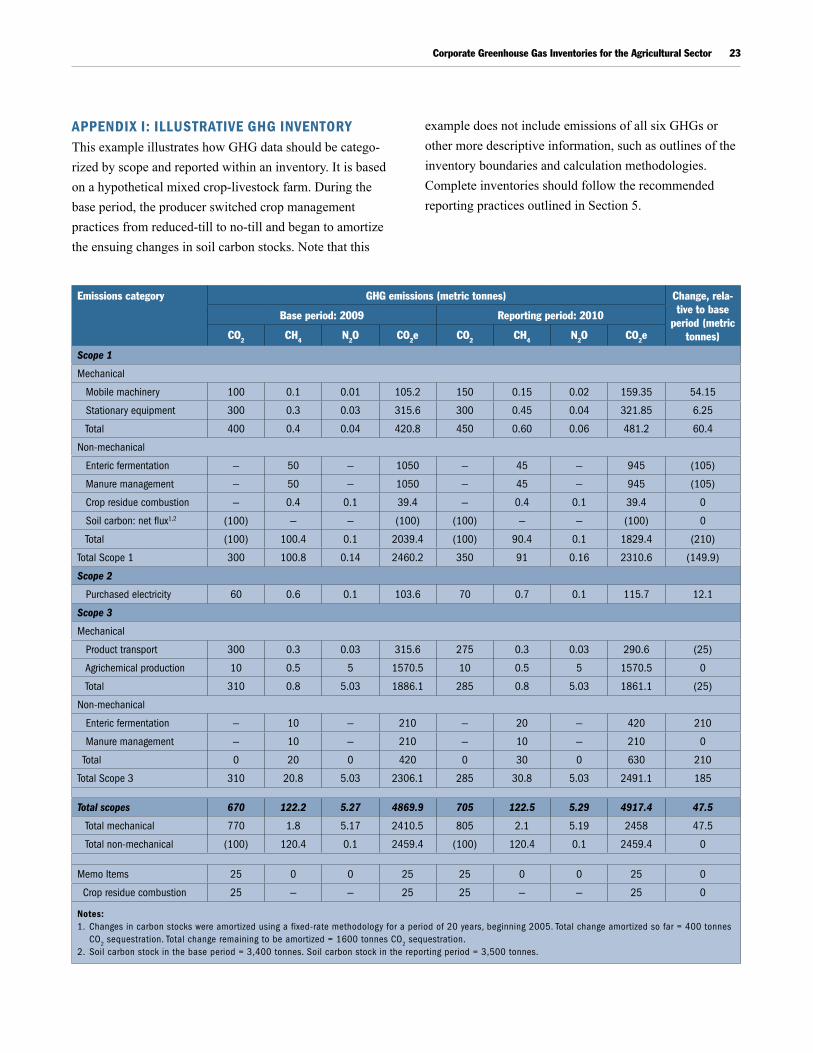
Corporate Greenhouse Gas Inventories for the Agricultural Sector 23
aPPendIx I: IllustratIve GhG Inventory This example illustrates how GHG data should be catego-rized by scope and reported within an inventory. It is based on a hypothetical mixed crop-livestock farm. During the base period, the producer switched crop management practices from reduced-till to no-till and began to amortize the ensuing changes in soil carbon stocks. Note that this
example does not include emissions of all six GHGs or other more descriptive information, such as outlines of the inventory boundaries and calculation methodologies. Complete inventories should follow the recommended reporting practices outlined in Section 5.
Emissions category GHG emissions (metric tonnes) Change, rela-tive to base
period (metric tonnes)
Base period: 2009 Reporting period: 2010
CO2 CH4 N2O CO2e CO2 CH4 N2O CO2e
Scope 1
Mechanical
Mobile machinery 100 0.1 0.01 105.2 150 0.15 0.02 159.35 54.15
Stationary equipment 300 0.3 0.03 315.6 300 0.45 0.04 321.85 6.25
Total 400 0.4 0.04 420.8 450 0.60 0.06 481.2 60.4
non-mechanical
enteric fermentation — 50 — 1050 — 45 — 945 (105)
Manure management — 50 — 1050 — 45 — 945 (105)
Crop residue combustion — 0.4 0.1 39.4 — 0.4 0.1 39.4 0
Soil carbon: net flux1,2 (100) — — (100) (100) — — (100) 0
Total (100) 100.4 0.1 2039.4 (100) 90.4 0.1 1829.4 (210)
Total Scope 1 300 100.8 0.14 2460.2 350 91 0.16 2310.6 (149.9)
Scope 2
Purchased electricity 60 0.6 0.1 103.6 70 0.7 0.1 115.7 12.1
Scope 3
Mechanical
Product transport 300 0.3 0.03 315.6 275 0.3 0.03 290.6 (25)
Agrichemical production 10 0.5 5 1570.5 10 0.5 5 1570.5 0
Total 310 0.8 5.03 1886.1 285 0.8 5.03 1861.1 (25)
non-mechanical
enteric fermentation — 10 — 210 — 20 — 420 210
Manure management — 10 — 210 — 10 — 210 0
Total 0 20 0 420 0 30 0 630 210
Total Scope 3 310 20.8 5.03 2306.1 285 30.8 5.03 2491.1 185
Total scopes 670 122.2 5.27 4869.9 705 122.5 5.29 4917.4 47.5
Total mechanical 770 1.8 5.17 2410.5 805 2.1 5.19 2458 47.5
Total non-mechanical (100) 120.4 0.1 2459.4 (100) 120.4 0.1 2459.4 0
Memo Items 25 0 0 25 25 0 0 25 0
Crop residue combustion 25 — — 25 25 — — 25 0
Notes: 1. Changes in carbon stocks were amortized using a fixed-rate methodology for a period of 20 years, beginning 2005. Total change amortized so far = 400 tonnes
CO2 sequestration. Total change remaining to be amortized = 1600 tonnes CO2 sequestration. 2. Soil carbon stock in the base period = 3,400 tonnes. Soil carbon stock in the reporting period = 3,500 tonnes.
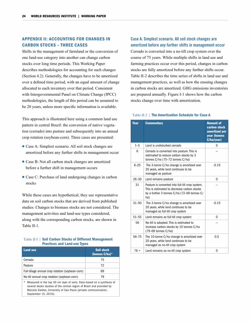
WORLD RESOURCES INSTITUTE | WORKING PAPER24
aPPendIx II: aCCountInG For ChanGes In Carbon stoCks – three CasesShifts in the management of farmland or the conversion of one land-use category into another can change carbon stocks over long time periods. This Working Paper describes methodologies for accounting for such changes (Section 4.2). Generally, the changes have to be amortized over a defined time period, with an equal amount of change allocated to each inventory over that period. Consistent with Intergovernmental Panel on Climate Change (IPCC) methodologies, the length of this period can be assumed to be 20 years, unless more specific information is available.
This approach is illustrated here using a common land use pattern in central Brazil: the conversion of native vegeta-tion (cerrado) into pasture and subsequently into an annual crop rotation (soybean-corn). Three cases are presented:
l Case A: Simplest scenario. All soil stock changes are amortized before any further shifts in management occur
l Case B: Not all carbon stock changes are amortized before a further shift in management occurs
l Case C: Purchase of land undergoing changes in carbon stocks
While these cases are hypothetical, they use representative data on soil carbon stocks that are derived from published studies. Changes to biomass stocks are not considered. The management activities and land-use types considered, along with the corresponding carbon stocks, are shown in Table II-1.
Case A: Simplest scenario. All soil stock changes are amortized before any further shifts in management occur Cerrado is converted into a no-till crop system over the course of 75 years. While multiple shifts in land use and farming practices occur over this period, changes in carbon stocks are fully amortized before any further shifts occur. Table II-2 describes the time series of shifts in land use and management practices, as well as how the ensuing changes in carbon stocks are amortized. GHG emissions inventories are prepared annually. Figure I-1 shows how the carbon stocks change over time with amortization.
Table II-I | Soil Carbon Stocks of Different Management Practices and Land-use Types
Land use Soil stock(tonnes C/ha)*
Cerrado 75
Pasture 72
Full-tillage annual crop rotation (soybean-corn) 69
no-till annual crop rotation (soybean-corn) 79
* Measured in the top 30 cm layer of soils. Data based on a synthesis of several dozen studies of the central region of Brazil and provided by Marcelo Galdos, university of Sao Paulo (private communication, September 15, 2010).
Table II-2 | The Amortization Schedule for Case A
year Commentary Amount of carbon stock amortized per year (tonnes C/ha/year)
1–5 land is undisturbed cerrado 0
6 Cerrado is converted into pasture. This is estimated to reduce carbon stocks by 3 tonnes C/ha (75–72 tonnes C/ha)
—
6–25 The 3-tonne C/ha change is amortized over 20 years, while land continues to be managed as pasture
-0.15
26–30 land remains pasture 0
31 Pasture is converted into full-till crop system. This is estimated to decrease carbon stocks by a further 3 tonnes C/ha (72–69 tonnes C/ha)
—
31–50 The 3-tonne C/ha change is amortized over 20 years, while land continues to be managed as full-till crop system
-0.15
51–55 land remains as full-till crop system 0
56 no-till is adopted. This is estimated to increase carbon stocks by 10 tonnes C/ha (79–69 tonnes C/ha)
—
56–75 The 10-tonne C/ha change is amortized over 20 years, while land continues to be managed as no-till crop system
0.5
76 + land remains as no-till crop system 0
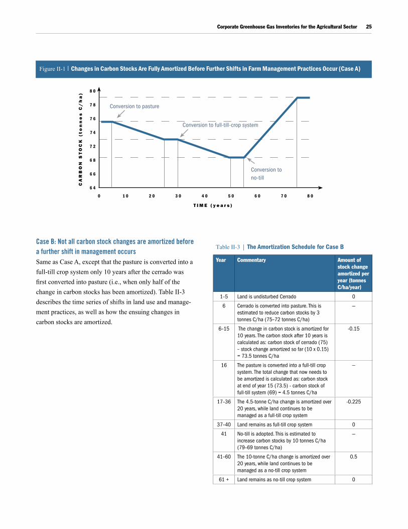
Corporate Greenhouse Gas Inventories for the Agricultural Sector 25
Case B: Not all carbon stock changes are amortized before a further shift in management occurs Same as Case A, except that the pasture is converted into a full-till crop system only 10 years after the cerrado was first converted into pasture (i.e., when only half of the change in carbon stocks has been amortized). Table II-3 describes the time series of shifts in land use and manage-ment practices, as well as how the ensuing changes in carbon stocks are amortized.
Conversion to pasture
ca
rb
On
st
Oc
k (
to
nn
es
c/
ha
)
t i m e ( y e a r s )
0
Figure II-1 | Changes in Carbon stocks are Fully amortized before Further shifts in Farm management Practices occur (Case a)
Conversion to no-till
Conversion to full-till-crop system
1 0 2 0 3 0 4 0 5 0 6 0 7 0 8 0
8 0
7 8
7 6
7 4
7 2
6 8
6 6
6 4
Table II-3 | The Amortization Schedule for Case B
year Commentary Amount of stock change amortized per year (tonnes C/ha/year)
1–5 land is undisturbed Cerrado 0
6 Cerrado is converted into pasture. This is estimated to reduce carbon stocks by 3 tonnes C/ha (75–72 tonnes C/ha)
—
6–15 The change in carbon stock is amortized for 10 years. The carbon stock after 10 years is calculated as: carbon stock of cerrado (75) – stock change amortized so far (10 x 0.15) = 73.5 tonnes C/ha
-0.15
16 The pasture is converted into a full-till crop system. The total change that now needs to be amortized is calculated as: carbon stock at end of year 15 (73.5) - carbon stock of full-till system (69) = 4.5 tonnes C/ha
—
17–36 The 4.5-tonne C/ha change is amortized over 20 years, while land continues to be managed as a full-till crop system
-0.225
37–40 land remains as full-till crop system 0
41 no-till is adopted. This is estimated to increase carbon stocks by 10 tonnes C/ha (79–69 tonnes C/ha)
—
41–60 The 10-tonne C/ha change is amortized over 20 years, while land continues to be managed as a no-till crop system
0.5
61 + land remains as no-till crop system 0
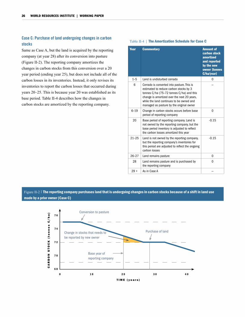
WORLD RESOURCES INSTITUTE | WORKING PAPER26
Case C: Purchase of land undergoing changes in carbon stocksSame as Case A, but the land is acquired by the reporting company (at year 28) after its conversion into pasture (Figure II-2). The reporting company amortizes the changes in carbon stocks from this conversion over a 20 year period (ending year 25), but does not include all of the carbon losses in its inventories. Instead, it only revises its inventories to report the carbon losses that occurred during years 20–25. This is because year 20 was established as its base period. Table II-4 describes how the changes in carbon stocks are amortized by the reporting company.
Table II-4 | The Amortization Schedule for Case C
year Commentary Amount of carbon stock amortized and reported by the new owner (tonnes C/ha/year)
1–5 land is undisturbed cerrado 0
6 Cerrado is converted into pasture. This is estimated to reduce carbon stocks by 3 tonnes C/ha (75–72 tonnes C/ha) and this change is amortized over the next 20 years, while the land continues to be owned and managed as pasture by the original owner
—
6–19 Change in carbon stocks occurs before base period of reporting company
0
20 Base period of reporting company. land is not owned by the reporting company, but the base period inventory is adjusted to reflect the carbon losses amortized this year
-0.15
21–25 land is not owned by the reporting company, but the reporting company’s inventories for this period are adjusted to reflect the ongoing carbon losses
-0.15
26–27 land remains pasture 0
28 land remains pasture and is purchased by the reporting company
0
29 + As in Case A —
Conversion to pasture
ca
rb
On
st
Oc
k (
to
nn
es
c/
ha
)
t i m e ( y e a r s )
0
Figure II-2 | the reporting company purchases land that is undergoing changes in carbon stocks because of a shift in land use made by a prior owner (Case C)
Purchase of landChange in stocks that needs to be reported by new owner
1 0 2 0 3 0 4 0
7 6
7 4
7 2
7 0
6 8
Base year of reporting company
Corporate Greenhouse Gas Inventories for the Agricultural Sector 27
Glossary
GHG-precursors Gases whose emissions lead to the formation of substances in the atmosphere with a climate change impact (e.g., SO2, NOX, NMVOC, and CO).
Global warming potential (GWP) The change in the climate system that would result from the emission of one unit of a given GHG compared to one unit of CO2.
Indirect GHG emissions Emissions that are a consequence of the operations of the reporting company, but that occur at sources owned or controlled by another company.
Land-use change The conversion of one category of land-use (e.g., forest) into another (e.g., cropland) through fire, draining, clear felling or soil preparation.
Mechanical sources (on farms) Equipment or machinery operated on farms, such as mobile machinery (e.g., harvesters), stationary equipment (e.g., boilers), and refrigeration and air-conditioning equipment. See also Non-mechanical sources.
Non-mechanical sources (on farms) Either bacterial processes shaped by climatic and soil conditions (e.g., decomposition) or the burning of crop residues. See also Mechanical sources.
Offset credits Tradable commodities that typically represent one metric tonne of CO2-equivalent emissions reductions or sequestration. In most cases, offset credits are generated at specific projects (offset projects).
Operational boundaries The boundaries that determine the direct and indirect emissions associated with operations owned or controlled by the reporting company.
Organizational boundaries The boundaries that determine the operations owned or controlled by the reporting company, depending on the consolidation approach taken (equity or control approach).
Product life cycle GHG inventory A compilation and evaluation of the inputs, outputs and the potential GHG impacts of a product – whether it be a good or a service – throughout its entire life cycle.
Ruminants Mammals that digest plant-based food by softening it within a first stomach (the ‘rumen’), then regurgitating the semi-digested mass (the ‘cud’) for further chewing. Enteric fermentation results from the microbial fermentation of food in the rumen. Examples of ruminants include cattle, goats, sheep, bison, yaks, water buffalo, and deer.
Scope Defines the operational boundaries in relation to direct and indirect GHG emissions.
Scope 1 Direct GHG emissions from sources owned or controlled by the reporting company.
Scope 2 Emissions associated with the generation of electricity, heating/ cooling, or steam purchased for the reporting entity’s own consumption.
Scope 3 Indirect emissions other than those covered in
scope 2.Volatilization of soil nitrogen The vaporization of soil NH3 and
NOX and their subsequent release into the atmosphere.
Accounting (GHG accounting) Quantification and organization of information about greenhouse gas (GHG) emissions (and carbon sequestration) based on common procedures, and correct attribution of the same to specific entities.
Agistment The practice of grazing one’s livestock on land controlled by another organization for the payment of a fee.
Agricultural products The outputs of agricultural and horticultural operations, including livestock, grains, vegetables, fruits and other crops.
Amortization The allocation of changes in carbon stocks (or emissions and sequestration data) over a period of time.
Base period A historic period (a specific year, series of consecu-tive years, or production season) against which a company’s emissions are tracked over time.
Biogenic CO2 emissions CO2 emissions from biological sources or materials derived from biological matter.
Carbon pools Natural stores of carbon in either biomass, soil matter, or harvested products. Carbon pools both take-up and release CO2.
Carbon sequestration The net carbon accumulation (i.e., CO2 fixation minus CO2 emissions) in carbon pools.
Carbon stocks The total amount of carbon stored on a plot of land at any given time in one or more carbon pools.
CO2-equivalent (CO2e) The universal unit for comparing emissions of different greenhouse gases, expressed in terms of the global warming potential (GWP) of one unit of CO2.
CO2 fixation The addition of carbon to carbon pools through photosynthesis.
CO2 flux The exchange of CO2 between carbon pools and the atmosphere, either through CO2 emissions or carbon sequestration.
Co-operative A business that is owned and controlled by the people (members) who use its services and whose benefits are shared by the members on the basis of use.
Corporate GHG emissions inventory A quantified list of the emissions from across the entire operations of a single company. Corporate inventories include the emissions of all six Kyoto GHGs (CO2, CH4, N2O, HFCs, PFCs, and SF6).
Crop year The period of time between two harvests. For many crops, this period approximates a calendar year, but for others several crop years may be possible each calendar year.
Direct GHG emissions Emissions from sources that are owned or controlled by the reporting company.
Emission factor A factor allowing GHG emissions to be estimated from a unit of available activity data (e.g., tonnes of fuel consumed, tonnes of product produced).
Enteric fermentation Fermentation that occurs in the digestive tracts of ruminant livestock species (e.g., cattle and sheep) and that releases CH4.
Greenhouse gases (GHGs) Gases that absorb and emit radiation at specific wavelengths within the spectrum of infrared radiation emitted by the Earth’s surface, the atmosphere, and clouds. The six main GHGs whose emissions are human-caused are: carbon dioxide (CO2); methane (CH4); nitrous oxide (N2O); hydrofluoro-carbons (HFCs); perfluorocarbons (PFCs); and sulphur hexafluo-ride (SF6).
WORLD RESOURCES INSTITUTE | WORKING PAPER28
notes1. Italicized terms are defined in the Glossary.2. The term agricultural products is used as a shorthand throughout the
text to describe these outputs.3. Available at: http://www.ghgprotocol.org/downloads/calcs/
Appendix_F_Leased_Assets.pdf. 4. The Corporate Standard uses the term ‘base year’ instead of
‘base period.’ The latter is preferred here because base periods may comprise more than one year and so the term ‘base year’ is potentially misleading.
5. See http://www.eia.doe.gov/oiaf/1605/. 6. See http://www.ipcc-nggip.iges.or.jp/public/2006gl/index.html. 7. See http://unfccc.int/national_reports/items/1408.php. 8. While the carbon in carbon stocks is contained within organic
compounds, stock size is measured in terms of the mass of that carbon alone. The amount of CO2 emitted/fixed from a change in carbon stock can be determined by multiplying the amount of stock change by 44/12, which is the ratio of the molecular weight of CO2
to
that of carbon.9. See http://unfccc.int/national_reports/annex_i_ghg_inventories/
items/2715.php.
reFerenCesBellarby, J., et al. (2008), Cool Farming: Climate Impacts of Agriculture
and Mitigation Potential, Greenpeace International, http://www.greenpeace.org/raw/content/ international/press/reports/cool-farming-full-report.pdf
Easterling, W.E., et al. (2007), “Food, Fibre and Forest Products,” in Climate Change 2007: Impacts, Adaptation and Vulnerability. Contribution of Working Group II to the Fourth Assessment Report of the Intergovernmental Panel on Climate Change, M.L. Parry et al., eds., Cambridge University Press, Cambridge, UK, 273-313
IPCC (2006), 2006 IPCC Guidelines for National Greenhouse Gas Inventories, IPCC National Greenhouse Gas Inventories Programme and Institute for Global Environmental Strategies, Japan, http://www.ipcc-nggip.iges.or.jp/public/index.html
Marshall, L., and A. Kelly (2010), The Time Value of Carbon and Carbon Storage: Clarifying the Terms and the Policy Implications of the Debate, WRI Working Paper, World Resources Institute, Washington, DC, http://www.wri.org/publications
Smith, P., D. Martino, and Z. Cai (2007), “Agriculture,” in Climate Change 2007: Mitigation. Contribution of Working Group III to the Fourth Assessment Report of the Intergovernmental Panel on Climate Change. B. Metz et al., eds., Cambridge University Press, Cambridge, UK, 497-540
U.S. EPA (2006a), Global Anthropogenic Non-CO2 Greenhouse Gas Emissions: 1990–2020, EPA 430-R-06-003, U.S. Environmental Protection Agency, Washington, DC, http://www.epa.gov/nscep/index.html
U.S. EPA (2006b), Global Mitigation of Non-CO2 Greenhouse Gas Emissions, EPA 430-R-06-003, U.S. Environmental Protection Agency, Washington, DC, http://www.epa.gov/nscep/index.html
about the authorStephen Russell is a Senior Associate in WRI’s Climate and Energy Program. E-mail: [email protected]; phone: (202) 729-7702.
aCknoWledGmentsThe author gratefully acknowledges the help and guidance of WRI colleagues throughout the production of this Working Paper, particularly Pankaj Bhatia, Laura Draucker, and Taryn Fransen for their expertise and thoughtful suggestions; Janet Ranganathan for her assis-tance with the review process; and Hyacinth Billings for managing the production process. The author also wishes to thank the many thought leaders who informed the analysis. Special thanks to Alexander Bjork, Marcelo Galdos, Daniella Malin, Michelle Perez, Richard Sheane, and Christof Walter for their review of this Working Paper.
This Working Paper would not have been possible without the generous support of the U.S. Agency for International Development and the Sea Change Foundation.
about WrIThe World Resources Institute is an environmental think tank that goes beyond research to find practical ways to protect the earth and improve people’s lives. Our mission is to move human society to live in ways that protect Earth’s environment for current and future generations.
Copyright 2011 World Resources Institute.
This work is licensed under the Creative Commons Attribution-NonCommercial-NoDerivative Works 3.0 License. To view a copy of the license, visit http://creative-commons.org/licenses/by-nc-nd/3.0/