Corporate Governance and Costs of Equity: Theory and Evidence∗

Di Li† Erica X. N. Li‡

October 8, 2013

Abstract

We propose an alternative explanation for the existence during 1990s and disappearance dur-ing 2000s of the governance-return relation. Using a real options model with managerialagency problem, we show that corporate governance mitigates investment distortions, eitherover- or under-investment, so that well governed firms have more valuable investment op-tions, present mainly during booms, and divestiture options, present mainly during busts,than poorly governed firms. Since investment options are riskier and divestiture options areless risky than assets-in-place, the mitigation of investment distortions generates the procycli-cal governance-return relation. Using governance index (G-index) and entrenchment index(E-index) as the measures of governance quality, we show that during the period of 1990-2007,well governed firms earn significantly higher returns during booms and lower returns duringbusts than poorly governed firms, controlling for various risk factors and firm characteristics.The results are robust to both aggregate and industry-specific business cycle classifications, toindustry-median adjusted returns, and to product market competition as alternative measureof governance.

JEL Classification: G1 G32 D92 E32Keywords: Corporate governance, managerial agency problem, stock returns, investment,business cycles

∗ This is a preliminary draft. Please do not cite or circulate without consent. The previous version of this paper iscirculated under the title “Does corporate governance affect the cost of equity capital?”. We thank Mike Barclay, JohnLong, Wei Yang, and especially Lu Zhang for their invaluable guidance. Comments and suggestions from Greg Bauer,Frederick Bereskin, Yangchun Chu, Fangjian Fu, Laura Liu, Jerold Warner, Charles Wasley, Yaxuan Qi, Chen Lin andseminar participants at London School of Economics, Pennsylvania State University, Stanford University, University ofRochester, University of Washington, University of Michigan, University of California at San Diego, and the WhartonSchool at the University of Pennsylvania are also gratefully acknowledged. All errors are our own.

† George State University, J. Mack Robinson College of Business Georgia State University, 35 Broad Street, Suite1201, Atlanta, GA 30303. E-mail: dili@gsu.edu; Tel: (404) 413-7320.

‡ Cheung Kong Graduate School of Business, Beijing, China, 100738; E-mail: xnli@ckgsb.edu.cn; Tel: (86)1085188888 exit 3075.

1 Introduction

Does corporate governance affect the costs of equity capital? Gompers, Ishii, and Metrick (2003)

(GIM) show that firms with stronger corporate governance earn higher average returns from

1990 to 1999. Core, Guay, and Rusticus (2006), however, find that this positive relation between

governance and returns is reversed from 2000 to 2003. Recent paper by Bebchuk, Cohen, and

Wang (2013) concludes that the association between governance and return disappears for the

sample from 2000 to 2008. They argue that the the disappearance is due to the over-valuation of

poorly governed firms before 2001 and the subsequent correction after market participants fully

recognized the negative effects of poor governance on firm value by the end of 2001. In this paper,

we propose an alternative explanation for the aforementioned existence and disappearance of

the governance-return relation. Using a real options model, we show that the effect of corporate

governance on stock returns is procyclical. In particular, strong governance leads to higher stock

returns during booms, but leads to lower stock returns during busts. Our empirical evidences

are consistent with the model predictions.

In the model, a manager is either an empire-builder or a shirker. In either case, the invest-

ment or divestiture decision is distorted: The former type tends to over-invest and is reluctant to

disinvest; the latter type avoids any effortful decisions, either investment or divestiture. Stronger

corporate governance makes any of these suboptimal investment behaviors costly to the man-

ager. The stronger the governance, the less distorted investment decisions made by the manager.

Therefore, the model predicts that, all else equal, a firm with stronger governance has more

valuable investment and divestiture options and hence higher firm value.

The paper’s most important insight is that the effect of corporate governance on stock returns

can be positive or negative, depending on economic fundamentals. Investment options allow

a firm to expand when the profitability is sufficiently high; thus, they are call options and are

riskier than the underlying assets. On the contrary, divestiture options are put options and are

less risky than the underlying assets because they give a firm options to scale down production

when profits are too low. Because a firm’s value consists of assets-in-place, investment options,

and divestiture options, its beta is a value-weighted average of the betas of the aforementioned

three parts. Therefore, all else equal, higher value of investment options, relative to the total

1

firm value, leads to higher expected stock returns, but higher value of divestiture options leads

to lower expected stock returns. As demonstrated in Figure 1, during boom periods when a

firm’s value consists mainly of investment options and assets-in-place, a well governed firm,

in contrast to a poorly governed firm, has more valuable investment options and consequently

higher expected returns. On the contrary, during busts when a firm’s value consists mainly of

divestiture options and assets-in-place, a well governed firm has more valuable divestiture op-

tions and lower expected returns. This intuition leads to the paper’s main hypothesis: corporate

governance affects stock returns positively during booms and negatively during busts. In other

words, the effect of corporate governance on the costs of equity capital is procyclical.

To verify the model’s predictions, we conduct a series of empirical tests. The key of the

tests are the measure of corporate governance strength and the classification of business cycles.

The two most used measures in the studies of the governance-return relation are governance

index (G-index) and entrenchment index (E-index). We follow the literature and use these two

as our main measures of governance strength. For robustness, we also repeat the tests using

product market competitiveness, measured by Herfindahl-Hirschman index (Herfindah, 1950;

Hirschman, 1945), as an alternative proxy for corporate governance.

Classifying business cycles in our context means identifying periods with high investment

opportunities, i.e., boom periods, and periods with high divestiture opportunities, i.e., bust peri-

ods. Since the pioneer work by Tobin (1969), Tobin’s average Q has been widely used as a proxy

for investment opportunities. It can also be shown that the relative importance of investment

and divestiture options to firm value is an increasing function of Tobin’s average Q in our model.

Therefore, we classify business cycles based on economy-wide Tobin’s average Q. We rank all

the quarters during 1990-2012 by their Tobin’s Q’s. The top 20% quarters with highest Tobin’s Q

are labeled as boom, the bottom 20% as bust, and the rest as normal. This procedure gives us a

classification of aggregate business cycles.

Past literature (see, Harford, 2005; Hoberg and Phillips, 2010, for example) has found that

investment opportunities faced by firms are not only affected by economy-wide conditions, but

also by industry-specific shocks. Industry-specific business cycles, although correlated, do not

exactly synchronize with each other. In extreme cases, boom for one industry can be bust for an-

2

other. 1 To measure investment opportunities more accurately, we also classify industry-specific

business cycles based on industry-level Tobin’s average Q.

The governance-return relation along business cycles is examined using both the time-series

portfolio approach and the cross-sectional characteristics approach for the period of 1990-2007,

during which both G-index and E-index are available. The portfolio approach examines the

returns of governance hedge portfolio based on G(E)-index, which longs the value-weighted

portfolio of firms with G(E)-index smaller than or equal to 5(0) and shorts the value-weighted

portfolio of firms with G(E)-index greater than or equal to 14(5). On average, return of gover-

nance hedge portfolio based on G-index is 0.71% per month (t-statistic = 3.22) during booms

and −1.08% per month (t-statistic = −1.08) during busts, controlling for market, size, value, and

momentum factors and with aggregate business cycles classification. The results remain sim-

ilar quantitatively and qualitatively for governance portfolio based on E-index and for returns

adjusted for industrial median. The statistically insignificant governance-return relation during

busts might be due to the inaccurately classified booms/busts.

To overcome this problem, we take the cross-sectional characteristics approach advocated

by Brennan, Chordia, and Subrahmanyam (1998) and regress individual stock returns on gov-

ernance indicator (one for strong governance and zero for weak governance) interacting with

boom, normal, and bust indicators, respectively, controlling for firm characteristics. Here, boom

(normal or bust) indicator can be based either on aggregate Tobin’s Q or on industry-specific

Tobin’s Q because it is defined as firm level. To implement the characteristics approach, we

use the clustered ordinary least squares assuming that variance of error terms is clustered in

time (month). Consistent with the model predictions, we find that on average, a well governed

firm outperforms (underperforms) an otherwise identical poorly governed firm during booms

(busts). In general, the results are more pronounced and more statistically significant if we clas-

sify business cycles with finer industry definitions. With G-index as the governance measure and

aggregate business cycles classification, a well governed company’s stock earns a monthly pre-

mium (discount) of 26 (149) basis points (t-statistic = 0.67 (1.71)) over a poorly governed firm’s

stock during booms (busts), controlling for an extensive set of firm characteristics used in Bren-

1The end of 1990s was a golden period for the IT industries but a difficult time for consumer non-durables industry.

3

nan, Chordia, and Subrahmanyam (1998). However, when business cycles are classified in Fama

and French (1997) 48-industry level, the monthly premium (discount) of the strong governance

stock becomes 69 (63) basis points (t-statistic = 2.03 (2.63)). The results are similar in magnitude

as well as statistical significance when E-index is used as the governance measure and when

returns are adjusted for industry median. With industry-specific business cycle classifications,

we also conduct the characteristics regressions using Fama and MacBeth (1973) method, 2 and

the results remain quantitatively similar.

We take several approaches to check the robustness of our empirical findings. First, we

utilize an alternative sample period and alternative cutoffs for the classification of business cycles.

Specifically, we identify Tobin’s Q cutoff points in a longer period from 1970 to 2012 and repeat

our empirical analysis. The results are essentially the same. We then changes the cutoffs of

boom/bust to top/bottom 30% and again obtain similar results to the benchmark ones. Second,

following Giroud and Mueller (2010, 2011), we use the product market competition, proxied by

the Herfindahl-Hirschman index (Herfindah, 1950; Hirschman, 1945) (HHI), as an alternative

measure of corporate governance. Because HHI is available in the longer period of 1970-2012,

we test our hypothesis in periods of 1990-2007 and 1970-2012 using HHI as governance measure

and find supportive results in both sample periods.

Finally, we address the possibility that the effective governance level is higher for firms with

higher G(E)-index during bust periods because those firms usually face harsher economic condi-

tions, which can serve as an external governance mechanism. We run cross-sectional regressions

of Tobin’s Q’s of equity on governance indicator interacting with boom, normal, and bust indica-

tors, controlling for firm characteristics. The results show that well governed firms (the ones with

low G(E)-index) are valued higher than poorly governed firms (the ones with high G(E)-index)

during both booms and busts. Therefore, the negative governance-return relation during busts

in our sample is not driven by the reversal of effective level of governance during busts.

Our paper belongs to the literature that studies the governance-return relation. We pro-

pose and test an alternative explanation for the positive governance-return relation in the 1990s

and its subsequent disappearance. Gompers, Ishii, and Metrick (2003) and Cremers, Nair, and

2With aggregate business cycle classification, there are only 2 bust quarters (8 bust months) and the results fromFama and MacBeth (1973) method have little power.

4

John (2009), among others, provide some explanations for the positive governance effect in the

1990s. Bebchuk, Cohen, and Wang (2013) documents the gradual recognition of the effects of

governance on firm value before 2002 by market participants, which, they argue, connects the

disappearance of the governance-return relation during 2000-2008. The misplacing of poorly

governed firms may have contributed to the positive governance-return relation found during

the 1990s. However, our study shows that even after market participants fully recognize the ef-

fects of governance on firm value, one should still observe positive (negative) governance-return

relation during boom (bust) periods. Therefore, this paper complements previous studies and

provide an alternative explanation.

This paper is related to Dow, Gorton, and Krishnamurthy (2005), who study the effect of

governance on bond pricing and term structure, and Albuquerque and Wang (2008), who study

the effect of country-level investor protection on equity risk premium and risk free rate. In

diverging from those studies, this paper builds on the studies of managerial agency problems

(Bertrand and Mullainathan, 2003; Hicks, 1935; Jensen, 1986, 1993) and focuses on the effect of

within-country firm-level governance on the cross-sectional stock returns. Finally, the paper is

related to the literature that studies the impact of corporate policies on cross-sectional stock

returns (e.g., Berk, Green, and Naik, 1999; Carlson, Fisher, and Giammarino, 2004; Zhang, 2005)

but with a focus on distorted investment policies.

The remainder of this paper is organized as follows. Section 2 presents a simple real options

model to provide intuition on the model’s main hypothesis. Sections 3 and 4 explain the data

sample and how to classify booms and busts. Section 5 presents empirical evidences on the

hypothesis. Section 6 concludes. Appendices A, B and C give the proofs of the lemmas.

2 Model

This section presents a real options model, following Dixit and Pindyck (1994), to illustrate the

impact of corporate governance on investment policies, firm value, and expected stock returns.

Assume that the Capital Asset Pricing Model (CAPM) holds in the economy and the market price

of risk is a constant, defined as φ. Consider a firm with N units of capital and the cash flow yt

5

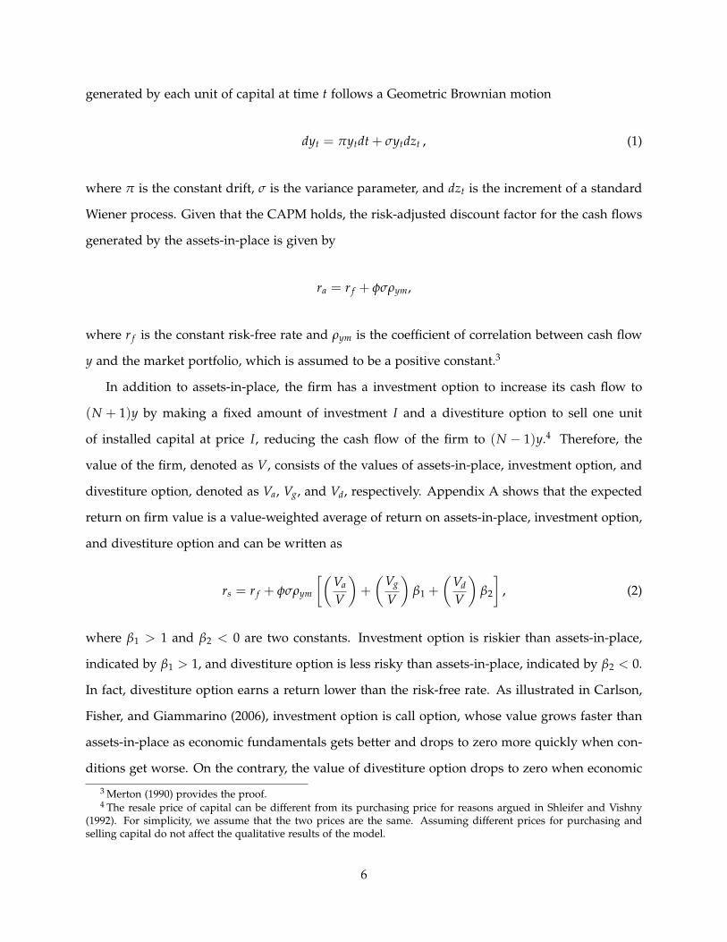
generated by each unit of capital at time t follows a Geometric Brownian motion

dyt = πytdt + σytdzt , (1)

where π is the constant drift, σ is the variance parameter, and dzt is the increment of a standard

Wiener process. Given that the CAPM holds, the risk-adjusted discount factor for the cash flows

generated by the assets-in-place is given by

ra = r f + φσρym,

where r f is the constant risk-free rate and ρym is the coefficient of correlation between cash flow

y and the market portfolio, which is assumed to be a positive constant.3

In addition to assets-in-place, the firm has a investment option to increase its cash flow to

(N + 1)y by making a fixed amount of investment I and a divestiture option to sell one unit

of installed capital at price I, reducing the cash flow of the firm to (N − 1)y.4 Therefore, the

value of the firm, denoted as V, consists of the values of assets-in-place, investment option, and

divestiture option, denoted as Va, Vg, and Vd, respectively. Appendix A shows that the expected

return on firm value is a value-weighted average of return on assets-in-place, investment option,

and divestiture option and can be written as

rs = r f + φσρym

[(Va

V

)+

(Vg

V

)β1 +

(Vd

V

)β2

], (2)

where β1 > 1 and β2 < 0 are two constants. Investment option is riskier than assets-in-place,

indicated by β1 > 1, and divestiture option is less risky than assets-in-place, indicated by β2 < 0.

In fact, divestiture option earns a return lower than the risk-free rate. As illustrated in Carlson,

Fisher, and Giammarino (2006), investment option is call option, whose value grows faster than

assets-in-place as economic fundamentals gets better and drops to zero more quickly when con-

ditions get worse. On the contrary, the value of divestiture option drops to zero when economic

3 Merton (1990) provides the proof.4 The resale price of capital can be different from its purchasing price for reasons argued in Shleifer and Vishny

(1992). For simplicity, we assume that the two prices are the same. Assuming different prices for purchasing andselling capital do not affect the qualitative results of the model.

6

fundamental is strong and goes up as it gets worse. Therefore, divestiture option serves as a

hedge for adverse economic conditions and earns lower expected returns.

Lemma 1 The expected return on firm value is positively related to the fraction of investment option value

to total firm value, Vg/V, and negatively related to the fraction of divestiture option value to total firm

value, Vd/V.

Lemma 1 builds on two basic results in the model: (1) investment option is call option and

is riskier than assets-in-place; (2) divestiture option is put option and is less risky than assets-

in-place. The value of investment option is positively correlated with the underlying economic

fundamentals and goes up faster than the value of assets-in-place when the fundamentals get

better. Because the return on firm value is the value-weighted average of returns on assets-in-

place, investment options, and divestiture options, all else equal, the expected return of the firm

is higher if a larger fraction of the firm value comes from its investment option. On the contrary,

the value of divestiture option is negatively correlated with fundamentals and has a negative

beta. All else equal, the expected return of the firm is lower if a larger fraction of the firm value

comes from its divestiture option.

Assume that the manager decides on the investment policies of the firm but his (her) incentive

is not perfectly aligned with that of outside shareholders. We consider two main agency prob-

lems discussed in the literature, empire-building (Albuquerque and Wang, 2008; Jensen, 1986,

1993) and shirking (Bertrand and Mullainathan, 2003; Hicks, 1935). We assume that for one unit

of investment made by the firm, the manager gains, per share of his ownership, additional B

units personal benefits net costs imposed by corporate governance. Stronger governance makes

suboptimal investment decisions more costly to managers and, all else equal, leads to lower ab-

solute value of B. A manager with a positive value of B is a empire-builder and the one with

a negative value of B enjoys quiet life. A manager with B = 0 has incentive perfectly aligned

with outside shareholders and there are no agency costs. To focus on the impact of suboptimal

investment decisions on firms’ stock returns, the manager’s private benefits are assumed to be

non-pecuniary and do not come from no outright appropriation of the firm’s cash flows. The

reduction in the firm’s value, therefore, comes entirely from the distorted investment policies.

7

The model also assumes that the manager and outside shareholders are subject to the same

stochastic discount factor, which may not be true for several reasons as studied in Chen, Miao,

and Wang (2010). This simplification hence ignores other agency problems such as compensation

with undiversifiable risk, which is beyond the scope of this paper. The following lemmas are

shown to hold under this simple setup. The proofs are relegated to Appendices A and B.

Lemma 2 Tobin’s average Q, defined as VNI , and values of investment and divestiture options decrease

with the absolute value of B.

Lemma 2 is quite intuitive. In the model, managers with empire building incentives tend

to advance investments and delay divestitures, while managers who prefer quiet life tend to

delay both investments and divestitures. Any deviation from optimal investment, either over-

or under-investment, reduces the values of investment/divestiture options and hence Tobin’s

average Q. Moreover, the larger the deviation, the lower the values of investment/divestiture

options and Tobin’s average Q. The absolute magnitude of B is positively related to the devia-

tion from optimal investment, therefore, negatively related to Tobin’s average Q and values of

investment/divestiture options. Based on lemmas 1 and 2, we derive our main hypothesis below.

Hypothesis 1 During periods when investment options are more important for firm value relative to

divestiture options, all else equal, firms with strong governance have higher expected returns than firms

with weak governance; during periods when divestiture options are more important, firms with weak

governance have higher expected returns than firms with strong governance.

The intuition behind the above hypothesis is as follows. As lemmas 2 and 1 indicate that

stronger governance leads to higher value of investment option and hence higher expected re-

turn on firm value, all else equal. However, stronger governance also leads to higher value of

divestiture option and hence lower expected return on firm value. The net effect of stronger

governance on firm’s stock return is positive when the value of investment option dominates

that of divestiture option and vice versa. Because the value of investment (divestiture) option

is positively (negatively) related to economic fundamentals, we hypothesize that all else equal,

firms with stronger governance have higher expected returns than firms with weaker governance

during booms, but lower expected returns during busts.

8

To summarize, the real options model implies that even though a firm with stronger gover-

nance always has a higher average Tobin’s Q than a firm with weaker governance, its expected

return is higher only when investment options are the important part of its firm value and lower

when divestiture options are the important part. In the next section, we empirically test this

hypothesis.

3 Classification of Business Condition

To test our hypothesis, we need to find an empirical proxy to measure the relative importance of

investment and divestiture options to firm value. The most widely used proxy in the literature

for investment opportunities is Tobin’s average Q. Tobin (1969) first proposes to use Tobin’s

average Q to measure firm’s incentive to invest in capital. Abel (1983) shows that the optimal

rate of investment depends on the marginal Q and Hayashi (1982) presents conditions under

which average Q and marginal Q are equal. Given that marginal Q is not observable, average Q

becomes widely used to measure firm’s growth opportunities.

In our model, the values of assets-in-place and investment options are positively related to

and the value of divestiture options is negatively related to economic fundamentals. It can be

shown that the ratio of investment to divestiture options is positively related to Tobin’s average

Q under the conditions that the risk premium of the firm is positive, or in another words, the

value of the firm positively co-moves with economic fundamentals.

Lemma 3 The ratio of investment and divestiture options Vg/Vd is an increasing function of Tobin’s

average Q as long as the firm has positive risk premium.

The proof of Lemma 3 is provided in Appendix C. Since majority of the firms in our sample

co-move positively with the market, we can use Tobin’s average Q to proxy for the relative

importance of investment and divestiture options, with high Tobin’s average Q indicating that

investment options are more important for firm value and low Tobin’s average Q indicating that

divestiture options are more important. To be concise, we omit the word “average” and use

Tobin’s Q to refer to Tobin’s average Q hereafter.

9

For each quarter, we calculate the total market value of assets for all companies in the COM-

PUSTAT/CRSP population at the quarter end. This market value of assets is particularly com-

puted as the market valuation of stocks plus the value of debt obtained from the companies

balance sheet. We then define the aggregate Tobin’s Q for the COMPUSTAT/CRSP population

as the ratio of the market value of assets to the total book value of assets of these companies in

the quarter. We further classify each quarter into three categories of business condition—boom,

normal, and bust—by comparing the value of Tobin’s Q with its historical value: A quarter is

labeled as boom (bust) if the Tobin’s Q of this quarter is above (below) the 80th (20th) percentile

of the ranked quarterly Q’s during the period 1990-2012, and a quarter is labeled as normal if it

is neither a boom nor bust.

Figure 2(a) illustrates the dynamics of the aggregate Tobin’s Q from 1990 to 2012. The graph

shows that during the 1990s, Tobin’s Q is relatively high, especially in the second half of the

1990s; Tobin’s Q experiences a sharp drop at the beginning of the 2000s and remains at a low

level in the first decade of the 2000s (relative to the 1990s), especially during the beginning and

the end of the 2000s.

It is well known that firm’s investment decisions are affected not only by broad economic

fundamentals but also by industry-specific technological/regulatory shocks (see Harford, 2005,

for example). Hoberg and Phillips (2010) show that industry-specific business cycles, although

correlated, do not perfectly synchronize with each other. Therefore, for a specific firm, the aggre-

gate Tobin’s Q might not be an accurate indicator for the amount of its investment opportunities.

To better capture the investment opportunities faced by firms, we classify firms into 10 and 48

industries, respectively, based on Fama and French (1997) and compute Tobin’s Q at the industry

level. Specifically, we calculate the total market value of assets for all companies in an industry

for each quarter as the market value of stocks plus the debt value from balance sheets of the

companies in that quarter. Then we compute Tobin’s Q of the industry by dividing the total

market value of assets in that industry by the total book value of assets of the industry at the

quarter end.

Figures 2(b) and 2(c) plot the time series of industry-level Tobin’s Q for the Fama and French

10 (FF10) industries and 48 (FF48) Industries. Consistent with previous evidences, the graphs

10

show that although Tobin’s Q’s of different industries exhibit similar cyclical movements, they

do not reach peaks and troughs at the exactly same quarters. In some extreme cases, the periods

that some industry experiences peak are the periods of trough for other industries. For example,

the end of 1990s was a golden period for the IT industries while the Tobin’s Q of consumer

non-durables industry reached its bottom.

To better understand the variations of aggregate and industry-level Tobin’s Q’s overtime,

Table 2 reports the number and the percentages of quarters labeled as “boom” and “bust” within

each year, respectively, between 1990-2012. Columns under “Pool” report statistics on boom/bust

classified based on the aggregate Tobin’s Q while columns under “FF10” and “FF48” report the

ones based on FF10 and FF48 industry classifications, respectively. We can see that based on

the aggregate Tobin’s Q, all the booms cluster within the period 1996-2001, during which 75% of

the quarters are classified as boom and none is classified as bust. On the contrary, for the same

period only 32.5% (25.35%) of the industry-quarters are booms and 7.5% (17.19%) are busts based

on the FF10 (FF 48) industry classification.5 Similarly, for the period of 2008 to 2012, 75% of the

quarters are busts and none is boom based on the aggregate Tobin’s Q, while 36% (23.02%) of

the industry-quarters are busts and 8.5% (15.31%) are booms based on the FF10 (FF48) industry

classification.

Based on the above observation, we conduct our empirical tests using both the aggregate

boom/bust classification and the industry-specific boom/bust classifications.

4 Data

Our sample includes all the companies for which corporate governance information from Risk-

Metrics is available. RiskMetrics publishes provisions of investor rights and takeover protection,

initially based on survey results from the Investor Responsibility Research Center (IRRC) that

was acquired by by ISS in 2005. IRRC/ISS has released eight volumes of such surveys (Septem-

ber 1990; July 1993; July 1995; February 1998; November 1999; February 2002; January 2004;

and January 2006). The surveys cover large companies in S&P 500 and the largest corporations

listed by Fortune, Forbes, and BusinessWeek, and starting 1998 the sample expanded to include

5 For the FF10 (FF48) industry classifications, there are 4× 10 (4× 48) industry-quarters within each year.

11

smaller firms and firms with high institutional ownership. In 2007 RiskMetricks changed the

survey methodology to meet ISS specifications and some variables needed for the construction of

governance indices were no long collected. Therefore our main sample ends in December 2007,

the last month before the new version of survey was conducted.

We use two indices to measure the effectiveness of corporate governance: governance index

(G-index) following Gompers, Ishii, and Metrick (2003), and entrenchment index (E-index) intro-

duced by Bebchuk, Cohen, and Ferrell (2009). Gompers, Ishii, and Metrick (2003) first introduce

the governance index using twenty-four provisions published by IRRC on investor rights and

takeover protection. This index is constructed by counting the number of such provisions that

apply to the company. Bebchuk, Cohen, and Ferrell (2009) investigate the twenty-four provisions

and identify six provisions that matter the most: staggered boards, limits to shareholder bylaw

amendments, poison pills, golden parachutes, and supermajority requirements for mergers and

charter amendments. They construct the E-index as the number of these six provisions that ap-

ply to the firm. We retrieve the G-index directly from RiskMetricks and construct the E-index

following Bebchuk, Cohen, and Ferrell (2009).

In Table 1 we report the summary statistics of governance index and entrenchment index.

The average G-index is 9.02 and the median is 9. For E-index, its mean is 2.31 and median is

2. We also report the distributions of these indices for each published volume. There are small

variations across releases but the distribution is overall very stable. Our summary statistics of G-

index and E-index are close to those reported by Gompers, Ishii, and Metrick (2003) and Bebchuk,

Cohen, and Ferrell (2009).

Because RiskMetrics does not publish volumes for each year, we follow Gompers, Ishii, and

Metrick (2003) and Bebchuk, Cohen, and Ferrell (2009) to assume that the corporate governance

measures of the covered companies remain unchanged between two consecutive releases. To

test our hypotheses, we match the sample with monthly stock return data from the Center for

Research in Security Prices (CRSP) and financial data from COMPUSTAT in annual and quarterly

frequencies.

12

5 Empirical Tests

In this section, we first present summary statistics on the governance-return relation and then

conduct rigorous empirical tests on Hypothesis ?. We use two different approaches to evaluate

the the governance-return relation along business cycles: the portfolio approach and the char-

acteristics approach. The first approach forms governance hedge portfolio based on E(G)-index

and measures the abnormal return of the governance portfolio along business cycles, controlling

for market, size, value, and momentum factors. The second approach examines the effect of

governance on individual firm returns along business cycles, controlling for various firm charac-

teristics.

5.1 Summary Statistics

To obtain a rough idea about the governance-return relation, we following Gompers, Ishii, and

Metrick (2003) and construct democracy portfolios, which contains firms with G(E)-index smaller

than or equal to 5(0) and dictatorship portfolios, governance hedge portfolios that contain firms

with greater than or equal to 14(5). The governance hedge portfolio, referred as G(E)-portfolio,

is then contracted by longing the G(E)-index based democracy portfolio and shorting the cor-

responding dictatorship portfolio. For each month, we calculate the value-weighted returns of

G- and E-portfolios, the time series of which are plotted in Figures 3(a) and 3(b) (in solid lines),

respectively. Consistent with our hypotheses, the figures show that during the second half of

the 1990s when investment opportunities are ample, the governance hedge portfolios yield more

positive returns than other periods; while in the beginning of the 2000s when it turns into busts

for investment, they experience more negative returns than other periods. In the same figures,

we also plot the series of returns of the governance hedge portfolios adjusted for the contempo-

raneous industry median (in dashed lines), with industries classified following Fama and French

(1997) 48-industry definition. The pattern of the industry-adjusted return series is the same.

The equal-weighted returns of the G- and E-portfolios are computed and plot them in Figures

3(c) and 3(d). They exhibit similar pattern as the series of returns to the governance hedge port-

folio. The return differences between strong and weak governance stocks are more pronounced

13

at the end of the 1990s and at the beginning of the 2000s, more likely to be positive in the for-

mer period and negative in the latter period. The industry-adjusted average return differences

between strong and weak governance stocks exhibit the same pattern.

In Table 3, we summarize average returns of the governance hedge portfolios during boom/bust/normal

periods, using both raw returns and returns adjusted by the corresponding Fama and French

(1997) 48-industry median returns. Results based on the aggregate boom/bust classification are

included in Panel A. We find that in the boom periods, the governance hedge portfolio yields

positive returns on average, 86 (107) basis points per month for raw returns of the G(E)-portfolio

and 149 (136) basis points per month for industry-adjusted returns of the G(E)-portfolio. The av-

erage value-weighted return of the G-portfolio is negative during busts, being −60 basis points

(bps) per month for raw returns and −26 bps for industry-adjusted returns. However, the average

return of the E-portfolio during busts is positive even though with a much smaller magnitude

compared to the average return during booms, being 24 bps per month for raw returns and 61

bps for industry-adjusted returns. The equal-weighted returns of the governance hedge portfolios

exhibit similar patterns as the value-weighted ones.

Table 2 shows that there are only 2 bust quarters (8 bust months) during the period 1990-2007

based on the aggregate business cycle classification, which gives low power to the statistics for

the bust periods. In Panels B and C of Table 3, we report the average return differences between

strong and weak governance stocks, based on FF10 and FF48 industry-specific business cycle

classifications, respectively. Here the industry-adjusted returns in Panels B and C are based on

10- and 48-industry classifications correspondingly. Under FF10 industry classification (Panel B),

the statistics show that strong governance stocks on average earn higher returns than weak gov-

ernance stocks in the boom periods. With industry median adjustment, this difference is 54 basis

points per month. For the bust periods, the average return difference between strong and weak

governance is negative for both governance measures and for both raw and industry-adjusted re-

turns, though the difference is smaller when E-index is used as the governance measure. Under

FF48 industry classification, the average return difference between strong and weak governance

stocks is positive during booms and the magnitude is large. For example, with G-index as the

governance measure, the difference in industry-adjusted returns is on average 97 bps each month.

14

In the bust periods, the average return difference is in general negative.

The study above does not consider the effects of other risks factors and firm’s characteristics

on returns. Next, we conduct rigorous statistical tests on the governance-return relation using

both the portfolio approach and the characteristics approach.

5.2 Portfolio Approach

In this subsection, we follow Gompers, Ishii, and Metrick (2003) and Bebchuk, Cohen, and Ferrell

(2009) taking a portfolio approach to test whether the risk-adjusted abnormal return based on

the governance trading strategy depends on business condition. Specifically, we employ the

standard four-factor model, that is, Fama and French (1993) three-factor model augmented by

the momentum factor of Carhart (1997).6

Without the dependence of the risk-adjusted abnormal return on business condition, the

standard four-factor model is estimated as

Rt = α + β1 × RMRFt + β2 × SMBt + β3 ×HMLt + β4 ×UMDt + εt, (3)

where Rt is the value-weighted excess return to the governance hedge portfolio in month t,

RMRFt is value-weighted market excess return in month t, SMBt (small minus big), HMLt (high

minus low), and UMDt (up minus down) are Fama and French (1993) three factors plus the

momentum factor in month t, measuring returns on zero-investment factor-mimicking portfolios

constructed to capture size, book-to-market (B/M), and momentum effect, respectively.

Gompers, Ishii, and Metrick (2003) use a sample up to 1999 and find that the governance

hedge portfolio (based on G-index) earns a positive abnormal return. We use the standard four-

factor model in equation (3) and the subsample up to 1999 to confirm this finding. The result in

reported in column 1 of Table 4. In Panel A, we run the test using raw returns, and in Panel B,

we use returns adjusted for contemporaneous median and industries classified following Fama

and French (1997) 48-industry definition. We find that indeed there is a positive abnormal return

(statistically significant at 10%) associated with the governance hedge portfolio. The abnormal

6 We obtain the factors from Kenneth French’s website.

15

return is also economically significant. The governance hedge portfolio earns an abnormal return

of 51 basis point per month for the raw-return specification and 46 basis points per month for the

industry-adjusted-return specification. Bebchuk, Cohen, and Ferrell (2009) measure governance

using E-index based a subset of the provisions used by Gompers, Ishii, and Metrick (2003),

and they also find that the governance hedge portfolio constructed using E-index earns positive

abnormal returns. Similarly, we estimate the standard four-factor model (3) using a subsample

up to 2003 that is used by Bebchuk, Cohen, and Ferrell (2009) and report the results in column 4

of Table 4. With E-index as the governance measure, we find that there is still a positive abnormal

return associated with the governance hedge portfolio and it has a larger magnitude as well as

more statistical significance.

The finding of superior abnormal returns earned by strong governance stocks has been chal-

lenged in the recent literature (Bebchuk, Cohen, and Wang, 2013; Core, Guay, and Rusticus, 2006).

Using a more updated sample, Bebchuk, Cohen, and Wang (2013) show that the superior per-

formance of the strong governance no longer exits especially after 2001, which the authors argue

to be attributed to the learning by investors of the mispricing. We run the standard four-factor

model (3) with the whole sample from 1990 to 2007. The results are reported in columns 2 (for

G-index) and 4 (for E-index) of Table 4. We find that using G-index as the governance measure,

the abnormal return on the governance hedge portfolio becomes much smaller and is no longer

statistically significant; using E-index as the governance measure, there is still a positive and

statistically significant abnormal return associated with the governance hedge portfolio. These

results are close to the findings of Bebchuk, Cohen, and Wang (2013).7

Our hypothesis states that the strong governance stocks are riskier than weak governance

stocks during boom periods while less risky during busts. Therefore, we hypothesize that the

governance hedge portfolio earns higher (lower) risk-adjusted abnormal returns during boom

(bust) periods. In other words, the abnormal return α varies in business condition. To test this

7 In Table 2 of Bebchuk, Cohen, and Wang (2013), they also find a positive and significant abnormal return onthe governance hedge portfolio for 1990 to 2008. The magnitude (69 basis points) is close to our finding of 66 basispoints. It is only in the subsample after 2001 do they find that strong governance stocks no longer outperform weakgovernance stocks.

16

hypothesis, we model α to depend on business condition:

Rt = αBM × IBMt + αNM × INM

t + αBT × IBTt

+ β1 × RMRFt + β2 × SMBt + β3 ×HMLt + β4 ×UMDt + εt, (4)

where IBMt , INM

t , and IBTt are binary variables indicating if month t is boom, normal, or bust

business condition, respectively. For example, if month t is bust, IBTt = 1; and if month t is not

bust, IBTt = 0.8 Our hypotheses hence predict αBM > 0 and αBT < 0. Since we have specifically

directional hypotheses, we conduct the statistical inference mainly using the p-value of one-sided

tests. In particular, for αBM being significantly different from zero, we care about whether it is

from the positive side instead of being from the negative side.

We run this test with the whole sample from 1990 to 2007 and report the results in columns

3 (for G-index) and 6 (for E-index) of Table 4. Because of our specifically directional hypotheses,

we report the p-values of the one-sided tests for αBM and αBT. In additional to the asterisks for

significance levels of the two-sided test, we use the bold fond to highlight the estimates of αBM

and αBT if they are statistically significant at 10 percent level for the one-sided tests.

Using G-index as the governance measure, in the raw-return specification, we find that

strong governance stocks outperform weak governance stocks during booms by 71 basis points

per month and underperform weak governance stocks during busts by 1.08 percentage points

monthly. The former is statistically significant at a one-sided p-value of 2.4 percentage points

while the latter is not as quite significant with a one-sided p-value of 14.1 percentage points.

From Table 2 we note that there are only two quarters in our sample period (September 1990 to

December 2007) that are bust. The lack of enough bust months may undermine the power of

the hypothesis test for αBT.9 With returns adjusted for contemporaneous median (using Fama

and French (1997) 48-industry definition), the estimated results are essentially the same. During

booms, strong governance stocks on average outperform weak governance stocks by a positive

8 Another way to test our hypotheses is to run the standard four-factor model (3) in boom, normal, and bustperiods separately. However, in our sample period (September 1990 to December 2007) there are only two quarters(eight months) that are bust. This makes the regression in the bust periods almost impractical.

9 One possibilility for the insignificance of αBT might be that during busts the agency conflict is not as severe asduring booms so that the governance does not make much difference in returns. However, the estimate of αBT is largein magnitude, which does not seem to support this argument.

17

and statistically significant abnormal return (95 basis points per month), while during busts,

weak governance stocks earn a superior abnormal return of 105 basis points per month though

not statistically significant.

The estimation results based on E-index as the governance measure are almost the same as

those based on G-index. Strong governance stocks outperform weak governance stocks during

boom periods by 119 basis points (96 basis points with industry adjustment) per month, and the

difference is highly statistically significant. During bust periods, though not statistically signifi-

cant, weak governance stocks on average outperform strong governance stocks by an abnormal

return of large magnitude—1.15 percentage points (87 basis points with industry adjustment)

per month.

Furthermore, the results above exhibit one interesting pattern for abnormal returns of gover-

nance hedge portfolio in the business cycles—abnormal returns of the governance hedge portfolio

are procyclical, that is, they are decreasing in the order of boom, normal, and bust periods. This

pattern echoes our theoretical predictions on the effect of governance on stock returns.

In all, the results based on the governance hedge portfolio and factor models are not incon-

sistent with our argument on the relation between governance and cost of equity. During boom

periods, strong governance increases the correlation between firms’ cash flow and business con-

dition. Therefore strong governance stocks require higher returns during boom periods. During

bust periods, strong governance reduces the association between cash flows and business con-

dition so that strong governance stocks earn lower returns. When the sample period consists

mostly of booms (i.e., Gompers, Ishii, and Metrick, 2003), it would seemingly suggest a positive

superior return associated with strong governance stocks. When boom and bust periods are both

included in the sample of study or if the investigation is not conditioned on business condition

(i.e., Bebchuk, Cohen, and Wang, 2013), the two opposite effects partly offset each other and it

would seemingly suggest no relation between governance and stock returns.

5.3 Characteristics Approach

Despite its popularity in empirical asset pricing studies, the factor approach is subject to some

caveats in our context. The portfolio approach can only be applied on the sample with boom/bust

18

classified based on aggregate business condition. With the economy-wide business cycle classi-

fication, the sample period covers only two bust quarters, which leads to low power for the test

of the governance-return relation during busts. Moreover, we show in Section 3 that the timings

of boom/bust periods for different industries exhibit variations in time. Therefore, it can imply

imprecise classification of business condition faced by companies and cause failure in detecting

the procyclical governance-return relation.

In this section, we adopt the characteristics approach pioneered by Brennan, Chordia, and

Subrahmanyam (1998) and conduct tests at the firm level. This approach is more suitable for

tests based on industry-specific business cycles because business condition indicators can now

be defined at the firm level. Moreover, including a large set of firm characteristics addresses

the concern of omitted variables bias since Gompers, Ishii, and Metrick (2003) find that firm

characteristics are correlated with the governance index.

The basis model for the characteristics approach is as follows

rit = a + bGit + cXit + eit, (5)

where, for firm i in month t, rit is the stock return, Git is the governance measure variable, Xit

is a vector of stock characteristics, and eit is the error term. To test our hypothesis that the effect

of governance on stock returns depends on business condition, we augment the basis model by

allowing the effect of governance, b, to vary along business cycles. Particularly, we assume that

b is a function of business condition, b = bBMIBMit + bNMINM

it + bBTIBTit , where IBM

it , INMit , and IBT

it

are business condition indicators for stock i in month t. Indicator IBMit equals one if month t is

a boom period for stock i and zero otherwise. Indicators INMit and IBT

it are defined similarly for

normal and bust periods, respectively.

Tests of asset pricing models with firm characteristics are usually conducted following Fama

and MacBeth (1973) two-pass procedure. In the first stage, equation (5) is estimated cross-

sectionally each month; in the second stage, the average of the coefficients and their standard

errors are obtained using the estimated time series (of boom, normal, and bust periods, respec-

tively) from the first stage. It is clear that Fama and MacBeth (1973) approach will have no power

19

for the tests during bust periods because there are only 2 bust quarters (8 bust months) in the

sample with aggregate business cycle classification. Petersen (2009) shows that both the clustered

ordinary least squares regression and Fama and MacBeth (1973) approach generate unbiased es-

timates of coefficients and standard errors if the sources of bias is cross-sectional dependence,

which applies here since stock returns exhibit little persistence in time but strong co-movement

in the cross section. More importantly, the clustered ordinary least squares regression suffers less

the problem of low power during busts in the aggregate business cycles classification. Therefore,

we choose the clustered ordinary least squares regression as our main method and repeat the

tests using Fama and MacBeth (1973) approach as a robustness check.

The empirical model of the characteristics regression is hence given by

rit = a + γt + bBM

(Git × IBM

it

)+ bNM

(Git × INM

it

)+ bBT

(Git × IBT

it

)+ cXit + eit, (6)

where γt is the fixed effect for month t and the error term eit is assumed to be clustered at

the monthly level, both of which are used to control for the cross-sectional dependence among

stocks. For stock characteristics, Xit, we use the same set of characteristics used by Brennan,

Chordia, and Subrahmanyam (1998) and Gompers, Ishii, and Metrick (2003), and the definition

and construction of these variables can be found in Appendix two of Gompers, Ishii, and Metrick

(2003). Our hypotheses state that bBM > 0 and bBT < 0.

We employ the panel sample from September 1990 to December 2007 and regress monthly

stock returns on interactions of governance measure SG and business condition controlling for

stock characteristics as shown in the model (6), where SG is a dummy indicating strong gov-

ernance that equals one if G(E)-index is smaller than or equal to 5(0) and zero if G(E)-index is

greater than or equal to 14(5). In the regressions, we include monthly fixed effects and allow the

error term to be cluster in time (month). The results are reported in Table 5. We start from busi-

ness cycles classified using COMPUSTAT/CRSP population and then we repeat the regression

using business cycles classified on the industry level using Fama and French 10- and 48-industry

definitions. For each specification, we conduct the regression with raw returns (reported in Panel

A) and repeat the regression using stock returns adjusted for contemporaneous industry median

20

(reported in Panel B). Again, since we have specifically directional hypotheses for bBM and bBT,

we conduct the statistical inferences using the p-values of one-sided tests. We report these one-

sided p-values for each regression and highlight the coefficient estimates of bBM and bBT with the

bold font if they are statistically significant at 10% for the one-sided tests.

Using the aggregate business cycles classification (columns 1 and 4), we find that strong

governance is associated with a positive coefficient in the boom periods and a negative coefficient

in the bust periods, though they are not statistically significant in general except for bBT when

G-index is the governance measure. Nevertheless, the magnitude of the coefficient estimates is

not trivial. For example, using E-index as the governance measure, under the aggregate business

cycles classification, everything else equal, during boom periods a strong governance stock is

estimated to earn 29 basis points (30 basis points with industry adjustment) more than a weak

governance stock per month, while during bust periods, a strong governance stock earns 46 basis

points (15 basis points with industry adjustment) less per month.

We show in Section 3 that the aggregate business cycles may not precisely capture the busi-

ness condition that stocks face as the timing of business condition for different industries exhibit

lags. This imprecision may dilute the estimated results for bBM and bBT. To address this concern,

we use industry-level business cycles classifications and repeat the regressions with business

cycles classified based on Fama and French 10- and 48-industries. In columns 2 and 5 when

industries are classified using Fama and French 10-industry definition and business cycles are

classified on the industry level, we find that the estimates of bBM and bBT become more statisti-

cally significant while their sign and magnitude remain as expected. For instance, using E-index

as the governance measure, based on raw stock returns, we find that during boom periods a

strong governance stock earns 45 basis points more than a weak governance stock per month.

This difference has a one-sided p-value of 0.07. We also find that in the bust periods, a weak

governance stock outperforms a strong governance stock by 57 basis points per month that is

statistically significant at a one-sided p-value of 0.009. The results are even more pronounced

with the industry-adjusted stock returns. With G(E)-index as the governance measure, we find

that during boom periods a strong governance stock outperform a weak governance stock by

74(89) basis points per month but underperforms during bust periods by 64(59) basis points per

21

month. All these coefficient estimates are statistically significant at the one-sided p-value of 0.04

at least.

We repeat the regressions in columns 3 and 6 with Fama and French (1997) 48-industry

classification and the corresponding industry-level business cycles classification. As expected,

with the refined industry and business cycles definition, the estimates of bBM and bBT are the

same in sign and stronger or similar in magnitude as in the regressions with Fama and French

10-industry definition (columns 2 and 5) but become more statistically significant with the one-

sided p-values being at most 0.022.

As a robustness check, we conduct Fama and MacBeth (1973) regressions with Fama and

French 10- and 48-industry classifications and the corresponding business cycles classifications

and the results are reported in Table 6. The results using the Fama and MacBeth (1973) approach

are essentially similar to those reported in columns 2-3 and 5-6 in Table 5. During boom (bust)

periods, a good (weak) governance stock outperforms a weak (good) governance stock in a non-

trivial magnitude for both G-index and E-index being the governance measure. While magnitude

of the coefficient estimates for bBM and bBT is similar, they are more statistically significant when

industries are classified more precisely and when industry-adjusted stock returns instead of raw

stock returns are used as the dependent variable.

In summary, the empirical study based on stock characteristics, complementing the results

based on governance hedge portfolio and factor models, is in general consistent with our hy-

potheses on the relation between governance and stock returns. We find that everything else

equal, strong governance stocks earn higher returns than weak governance stocks during boom

periods and lower returns during bust periods. Moreover, consistent with our finding in Section

3 on business cycles, the more precisely the industries are classified, the more pronounced and

statistically significant the results are, especially when the dependent variable is the industry-

adjusted stock return.

5.4 Robustness

In the previous subsections, we test the hypotheses on the relation between governance and

stock returns, and we find that this relation depends on business cycles. In this subsection,

22

we provide several robustness tests to strengthen our findings. Below, we first utilize alternative

criteria for the classification of business condition, then we use product market competition as the

governance measure to test if our argument survives under the alternative governance measure,

and finally, we study the effect of governance on stock valuation and check if our findings during

busts are driven by the reversal of the effective level of governance.

5.4.1 Alternative Criteria of Business Cycles Classification

We classify business condition using quarterly Tobin’s Q of assets of a sample from 1990 to 2012.

By doing so, we ensure that there is boom and bust periods in our testing period. However, since

the classification of business cycles (boom and bust) is based on a relative sense. That is, boom

(bust) periods are those quarters with aggregate or industry-level Tobin’s Q in its top (bottom)

twenty percent in this sample period (1990-2012), the classification of business cycles might be

sensitive to the sample period used. To address this concern, we extend the sample period

used for business condition classification to the longest period available to construct quarterly

Tobin’s Q of assets, that is, 1970-2012. The drawback of this extension is that all aggregate busts

classified using the longer sample are outside of the testing sample period (September 1990 to

December 2007), and hence our robustness tests with the longer sample period for business

condition classification have to be based on industry business cycles.

We repeat the regressions in Subsection 5.3. In columns 1-4 of Panels A and B of Table 7, we

use clustered OLS method (A for raw returns and B for industry-adjusted returns), and in the

same columns of Panels C and D, we use Fama and MacBeth (1973) method (C for raw returns

and D for industry-adjusted returns). To save space, we only report the estimation results of bBM

and bBT as well as their one-sided p-values.

Basically, with business cycles classified using a longer sample of Tobin’s Q, we still find a

premium during booms and a discount during busts for returns of strong governance stocks.

The magnitude of the stock return differences is nontrivial and is close to those found in the

basis analysis in Subsection 5.3. The coefficient estimates of bBM and bBT are also statistically

significant for one-sided tests in most cases. Therefore, our argument seems to be robust to the

alternative sample periods for business condition classification.

23

We classify booms and busts using the cutoffs of top and bottom twentieth percentiles of

Tobin’s Q in our basis analysis. One might be concerned about the robustness of these cutoffs.

We hence amend the criteria for booms and busts by widening the range of booms and busts to

the top and bottom thirty percent of Tobin’s Q. Similarly, we repeat the regressions in Subsection

5.3. For clustered OLS (Panels A and B of Table 7), we are able to run the regressions with the

aggregate classification of business cycles while we cannot do so with Fama and MacBeth (1973)

method (Panels C and D).

With business cycles classified based on a wider range, the findings based on the aggregate

business condition indicate a premium during booms and a discount during busts for strong

governance stocks though these estimates are almost insignificant statistically and in magnitude

in most cases. This is probably because, with a wider range for booms and busts, the effect is

somewhat diluted, especially when these effect is not quite significant in the basis analysis with

aggregate business cycles. Similar to the basis analysis, when we classify business cycles based

on industries, the governance effect becomes more pronounced and more statistically significant.

We find premiums during booms and discounts during busts for strong governance stocks.10

The magnitude of these effects are nontrivial, and they are in general statistically significant for

the corresponding one-sided tests, especially when industries are classified following the finer

Fama and French (1997) 48-industry definition and when industry-adjusted returns are used as

the dependent variables.

In short, our findings are robust to alternative criteria for the classification of business cycles,

with which we can still find strong governance stocks in general earn higher returns during

boom periods and lower returns during bust periods than weak governance stocks.

5.4.2 Alternative Measure of Governance and Extended Sample Period

G-index and E-index are constructed using the provisions of corporate charters or state laws that

protect managers. The less protection corporate managers enjoy, the less likely the managers

distort the investment decision. However, the absence of protection provisions is by no means

10 The only exception is the in column 6 of Panel C when raw return is the dependent variable, industries areclassified using Fama and French 10-industry definition, and Fama and MacBeth (1973) method is used for theregression. In that, the coefficient estimate of bBT is positive but very tiny and statistically insignificant.

24

the only source of pressure that disciplines corporate managers. Giroud and Mueller (2010, 2011)

document that firms benefit from strong corporate governance (measured by passage of business

combination laws and G-index), in terms of equity returns, firm value, and operating productiv-

ity and performance, but only when they operate in the non-competitive industries. Therefore,

product market competition to some extent plays a similar role of corporate governance that

mitigates distortions in managerial decisions. We hence expect to observe similar effect of prod-

uct market competition on cost of equity. That is, else equal, stocks of companies operating

in competitive industries earn higher (lower) returns than stocks of companies in concentrated

industries in the boom (bust) periods.

To test this hypothesis, we retrieve sales data from COMPUSTAT and construct the Herfindahl-

Hirschman index (Herfindah, 1950; Hirschman, 1945), or HHI. We then classify governance in

the broad sense with HHI. A company is thought to be well (poorly) governed if the HHI of the

industry in which this company operates is below (above) the contemporaneous bottom (top)

quartile. We follow Fama and French (1997) 48-industry definition to classify industries. With

the alternative governance measure, we repeat the regression 6 and report the results in Table 8.

In Panel A of Table 8, we use the sample of Tobin’s Q from 1990 to 2012 for business cycles

classification, and our regression sample is from 1990 to 2011 since HHI data is available after

2007. This sample period of the regressions covers the bust periods following the financial crisis

in 2008. Inclusion of these periods makes our findings less subject to the concern that the pattern

of stock returns in the period 1990-2007 happens to match with our argument. With the clustered

ordinary least squares (columns 1-2), we find that in the boom periods, stocks of companies in

competitive industries earn average 33 basis points (34 basis point for industry-adjusted returns)

more per month than those in concentrated industries; but during bust periods, stocks of compa-

nies in non-competitive industries outperform those in competitive industries by 53 basis points

(66 basis points for industry-adjusted returns) per month. All of these differences are statistically

significant with one-sided p-values no larger than 0.02. In columns 3-4 of Panel A, we provide the

regression results based on Fama and MacBeth (1973) method. The results are similar to those

based on the clustered ordinary least squares.

Since HHI can be calculated for a longer period of time, we also test the hypothesis using

25

business cycles classified with the longer sample of Tobin’s Q from 1970 to 2012. With business

cycles information earlier than 1990, we are able to run the regression 6 in a sample from 1975

to 2011. With the data before 1990 and after 2007 in the regression, the findings are more robust

to the sample period. Results based on the clustered ordinary least squares indicate that during

boom periods, stocks in competitive industries outperform stocks in concentrated industries dur-

ing boom periods by 48 basis points (27 basis points for industry-adjusted returns) per month;

during bust periods, stocks in concentrated industries earn 74 basis points (58 basis points for

industry-adjusted returns) more per month. Again, these differences are statistically significant

with p-values all close to zero. We confirm these findings using Fama and MacBeth (1973) method

and the results (reported in columns 3-4 of Panel B) are essentially the same.

As a summary, using the product market competition as the alternative measure of gover-

nance, consistent to our hypotheses, we still find that stocks of well-governed companies earn

higher returns during boom periods and lower returns during bust periods compared to stocks

of poorly-governed companies.

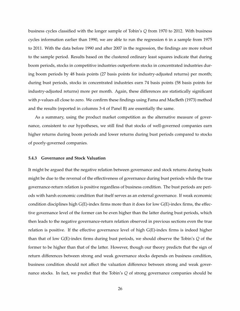
5.4.3 Governance and Stock Valuation

It might be argued that the negative relation between governance and stock returns during busts

might be due to the reversal of the effectiveness of governance during bust periods while the true

governance-return relation is positive regardless of business condition. The bust periods are peri-

ods with harsh economic condition that itself serves as an external governance. If weak economic

condition disciplines high G(E)-index firms more than it does for low G(E)-index firms, the effec-

tive governance level of the former can be even higher than the latter during bust periods, which

then leads to the negative governance-return relation observed in previous sections even the true

relation is positive. If the effective governance level of high G(E)-index firms is indeed higher

than that of low G(E)-index firms during bust periods, we should observe the Tobin’s Q of the

former to be higher than that of the latter. However, though our theory predicts that the sign of

return differences between strong and weak governance stocks depends on business condition,

business condition should not affect the valuation difference between strong and weak gover-

nance stocks. In fact, we predict that the Tobin’s Q of strong governance companies should be

26

always higher than that of weak governance companies, independent of business cycles. There-

fore, we can test this alternative argument for the findings during busts by investigating the

valuation of strong and weak governance stocks along business cycles. In this section, we show

that during both boom and bust periods, Tobin’s Q of strong governance firms is greater than

that of weak governance firms.

To gain a rough idea, we construct the valuation of stocks as equity Tobin’s Q, the ratio of

the market value of stocks at the quarter end to the book value of common stocks in the quarter.

Similar to return differences between strong and weak stocks, we plot the series of valuation dif-

ferences in Figure 3(e) and 3(f) (in solid lines), with G-index and E-index as governance measure,

respectively. Consistent with our argument, the figures show that the difference in stock valua-

tion is always positive. Compared with returns, valuation appears more industry clustering. To

account for the valuation difference in the industry level, we construct industry-adjusted Q of

the stocks by subtracting the contemporaneous industry median of Q of the stocks, using Fama

and French (1997) 48-industry classification for the industry definition. We plot the series of

industry-adjusted Q’s in the same figures in dashed lines. The figures again show that measured

with industry-adjusted Q, strong governance companies’ stocks are always priced higher than

stocks of weak governance companies.

Similar to returns, we summarize the average valuation difference between strong and weak

governance stocks in Table 3. Except for the case in which business condition is classified on

Fama and French 10-industry level and governance is measured with E-index (Panel B), strong

governance stocks are all valued higher than weak governance stocks regardless of the business

condition. Therefore, though stock valuation measure, Q, is highly positively correlated to To-

bin’s Q of firm assets that is used to classify business cycles, we do not observe the procyclical

pattern for the difference in stock valuation between strong and weak governance stocks.

We establish the relation between governance and stock valuation by putting the hypothesis to

multivariate regressions. We take the same valuation regression specification used by Gompers,

Ishii, and Metrick (2003) as the basis model and augment it to allow the governance effect to vary

27

in business cycles:

Qit = a + γt + bBM

(Git × IBM

it

)+ bNM

(Git × INM

it

)+ bBT

(Git × IBT

it

)+ cZit + eit, (7)

where Qit is the Tobin’s Q of company i’s stock in quarter t, γt is the fixed effect and the error

term eit is clustered in quarters; IBMit , INM

it , and IBTit are binary variables indicating the business

condition that company i is experiencing in quarter t. For example, IBMit = 1 if company i

is during boom in quarter t, and IBMit = 0 if otherwise. As for the control variables, Zit, we

follow Gompers, Ishii, and Metrick (2003) and include firm size as the logarithm of the book

value of assets, firm age as the logarithm of the number of years as of December of the data

year in the COMPUSTAT/CRSP database, a dummy variable indicating whether the company

is incorporated in the state of Delaware, and a dummy variable indicating whether the stock is

included in the S&P 500 index. To test that the hypotheses that stock valuation is higher for

strong governance stocks both during boom and bust periods, we report the p-values of the one-

sided tests and highlight the coefficient estimates of bBM and bBT using the bold font if they are

statistically significant in the one-sided tests at 10% level at least.

Same as the study on stock returns, we start from the regression of the model (7) under

the aggregate business cycles classification. The results are reported in columns 1 and 4 of

Table 9, Panel A for raw value of Q and Panel B for industry-adjusted Q. We find that indeed,

strong governance stocks are associated with higher stock valuation during boom and normal

periods. For example, with G(E)-index as the governance measure, a strong governance stock is

priced 56(68) cents higher for every dollar of book value than a weak governance stock during

boom periods, and the premium is 32(28) cents per dollar of book value in normal periods.

The valuation differences during boom and normal periods are highly statistically significant

with one-sided p-values close to 0.000. During bust periods, however, the difference in stock

valuation between strong and weak governance stocks is tiny and statistically insignificant. This

insignificant difference in the bust periods again might be due to the imprecision of business

condition classification and the limited number of bust quarters in the sample. This problem of

few bust quarters in the sample is more severe because the regression of stock valuation is in the

28

quarterly frequency. The results based on industry-adjusted Q is very close to those based on

raw Q.

To classify business cycles more precisely, we repeat the stock valuation regression with Fama

and French 10-industry definition and corresponding industry-level business cycles. The results

are reported in columns 2 and 5 of Table 9. Indeed, with a refined industry-level business cycles

classification, we find that valuation of strong governance stock is always higher than that of

weak governance stocks. With Fama and French 10-industry definition, using G(E)-index as the

governance measure, a strong governance stock enjoys premiums of 37(41) cents, 40(39) cents,

and 27(29) cents per dollar of book value during boom, normal and bust periods, respectively,

compared to a weak governance stock. All these premiums are highly statistically significant

with one-sided p values smaller than 0.01. With industry-adjusted Q, the results are essential

the same. The differences in stock valuation between strong and weak governance stocks in all

business condition are positive in non-trivial magnitude and are highly statistically significant

with p-values all close to 0.000. Again, we refine the industry classification following Fama and

French (1997) 48-industry definition and classify industry-level business cycles accordingly, and

then we repeat the valuation regression and report the results in columns 3 and 6 of Table 9. These

results are almost indifferent to those under Fama and French 10-industry classification. They

once more confirm that strong governance stocks are always priced higher than weak governance

stocks.

We also conduct the multivariate analysis of stock valuation using Fama and MacBeth (1973)

method to confirm our findings from the clustered ordinary least squares. Same as stock returns,

we only run Fama and MacBeth (1973) regressions under industry business cycles due to the

problem of limited number of bust quarters in the sample under the aggregate business cycles

classification. We report the results from Fama and MacBeth (1973) regressions in Table 10. These

results are very close to those based on the clustered OLS with industry business cycles, both in

magnitude and statistical significance.

In all, we find that, in contrast to the relation between governance and stock returns, the

effect of governance on stock valuation is independent of business cycles. All else equal, a strong

governance stock enjoys a price premium over a weak governance stock regardless of business

29

condition. Therefore, our findings of bust periods do not seem to be driven by the reversal of the

effective governance level during busts.

6 Conclusion

The paper provides an alternative explanation of the governance-return relation. Based on the

assumption that corporate governance alleviates agency problems caused by the empire-building

or shirking incentives of managers, we show that firms with stronger governance, all else equal,

have less distorted investment policies, higher values of investment and divestiture options, and

higher Tobin’s Q. Most importantly, those firms have higher expected returns during booms but

lower expected returns during busts compared to firms with weaker governance.

We test our model predictions using a sample from 1990 to 2007. We first classify the business

condition (boom, normal, and bust) facing firms based on the aggregate and industry-level To-

bin’s Q’s. Then we study the effects of governance on stock returns along business cycles. With

G-index and E-index as the measures of governance, consistent with our model predictions, we

find that well governed firms earn higher returns than poorly governed firms during booms, but

they earn lower returns during busts.

The procyclicality of the governance-return relation provides a coherent explanation to the

documented findings on the existence and disappearance of the effect of governance on stock

returns. More importantly, our findings suggest that corporate governance does affect the cost of

equity, however, in a subtle way.

30

References

Abel, Andrew B. 1983. “Optimal Investment under Uncertainty.” American Economic Review73 (1):228–233.

Albuquerque, Rui and Neng Wang. 2008. “Agency Conflicts, Investment, and Asset Pricing.”Journal of Finance 63 (1):1–40.

Bebchuk, Lucian, Alma Cohen, and Allen Ferrell. 2009. “What Matters in Corporate Gover-nance?” Review of Financial Studies 22 (2):783–827.

Bebchuk, Lucian A., Alma Cohen, and Charles C.Y. Wang. 2013. “Learning and DisappearingAssociation between Governance and Returns.” Journal of Financial Economics 108 (2):323–348.

Berk, Jonathan B., Richard C. Green, and Vasant Naik. 1999. “Optimal Investment, GrowthOptions, and Security Returns.” Journal of Finance 54 (5):1553–1607.

Bertrand, Marianne and Sendhil Mullainathan. 2003. “Enjoying the Quiet Life? Corporate Gov-ernance and Managerial Preferences.” Journal of Political Economy 111 (5):1043–1075.

Brennan, Michael J., Tarun Chordia, and Avanidhar Subrahmanyam. 1998. “Alternative Fac-tor Specifications, Security Characteristics, and the Cross-Section of Expected Stock Returns.”Journal of Financial Economics 49 (3):345lC373.

Carhart, Mark M. 1997. “On Persistence in Mutual Fund Performance.” Journal of Finance52 (1):57–82.

Carlson, Murray, Adlai Fisher, and Ron Giammarino. 2004. “Corporate Investment and AssetPrice Dynamics: Implications for the Cross-section of Returns.” Journal of Finance 59 (6):2577–2603.

———. 2006. “Corporate Investment and Asset Price Dynamics: Implications for SEO EventStudies and Long-Run Performance.” Journal of Finance 61 (3):1009–1034.

Chen, Hui, Jianjun Miao, and Neng Wang. 2010. “Entrepreneurial Finance and NondiversifiableRisk.” Review of Financial Studies 23 (12):4348–4388.

Core, John E., Wayne R. Guay, and Tjomme O. Rusticus. 2006. “Does Weak Governance CauseWeak Stock Returns? An Examination of Firm Operating Performance and Investors’ Expecta-tions.” Journal of Finance 61 (2):655–687.

Cremers, K. J. Martijn, Vinay B. Nair, and Kose John. 2009. “Takeovers and the Cross-Section ofReturns.” Review of Financial Studies 22 (4):1409–1445.

DeMarzo, Peter, Mike Fishman, Zhiguo He, and Neng Wang. 2012. “Dynamic Agency and the qTheory of Investment.” Journal of Finance 67 (6):2295lC2340. Manuscript.

Dixit, Avinash K. and Robert S. Pindyck. 1994. Investment Under Uncertainty. Princeton, NJ:Princeton University Press.

Dow, James, Gary B. Gorton, and Arvind Krishnamurthy. 2005. “Equilibrium Investment andAsset Prices under Imperfect Corporate Control.” American Economic Review 95 (3):659–681.

31

Fama, Eugene F. and Kenneth R. French. 1993. “Common Risk Factors in the Returns on Stocksand Bonds.” Journal of Financial Economics 33 (1):3–56.

———. 1997. “Industry Costs of Equity.” Journal of Financial Economics 43 (2):153–193.

Fama, Eugene F. and James D. MacBeth. 1973. “Risk, Return, and Equilibrium: Empirical Tests.”Journal of Political Economy 81 (3):607–636.

Giroud, Xavier and Holger M. Mueller. 2010. “Does Corporate Governance Matter in CompetitiveIndustries?” Journal of Financial Economics 95 (3):312–331.

———. 2011. “Corporate Governance, Product Market Competition, and Equity Prices.” Journalof Finance 66 (2):563–600.

Gompers, Paul A., Joy Ishii, and Andrew Metrick. 2003. “Corporate Governance and EquityPrices.” Quarterly Journal of Economics 118 (1):107–155.

Harford, Jarrad. 2005. “What Drives Merger Waves?” Journal of Financial Economics 77 (3):529–560.

Hayashi, Fumio. 1982. “Tobin’s Marginal q and Average q: A Neoclassical Interpretation.” Econo-metrica 50 (1):213–224.

Herfindah, Orris C. 1950. Concentration in the U.S. Steel Industry. Dissertation, Columbia Univer-sity.

Hicks, John R. 1935. “Annual Survey of Economic Theory: The Theory of Monopoly.” Economet-rica 3 (1):1–20.

Hirschman, Albert O. 1945. National Power and the Structure of Foreign Trade. Berkeley and LosAngeles, CA: University of California Press.

Hoberg, Gerard and Gordon Phillips. 2010. “Real and Financial Industry Booms and Busts.”Journal of Finance 65 (1):45–86.

Jensen, Michael C. 1986. “Agency Costs of Free Cash Flow, Corporate Finance and Takeovers.”American Economic Review 76 (2):323–329.

———. 1993. “The Modern Industrial Revolution, Exit, and the Failure of Internal Control Sys-tems.” Journal of Finance 48 (3):831–880.

Merton, Robert C. 1990. Continuous-Time Finance. Malden, MA: Blackwell Publishing.

Nikolov, Boris and Toni M. Whited. 2013. “Agency Conflicts and Cash: Estimates from a DynamicModel.” Journal of Fina Forthcoming.

Petersen, Mitchell A. 2009. “Estimating Standard Errors in Finance Panel Data Sets: ComparingApproaches.” Review of Financial Studies 22 (1):435–480.

Shleifer, Andrei and Robert W. Vishny. 1992. “Liquidation Values and Debt Capacity: A MarketEquilibrium Approach.” Journal of Finance 47 (4):1343–1366.

Tobin, James. 1969. “A General Equilibrium Approach to Monetary Theory.” Journal of Money,Credit, and Banking 1:15–29.

Zhang, Lu. 2005. “The Value Premium.” Journal of Finance 60 (1):67–103.

32

Appendix

A Proof of Lemma 1

Given that the CAPM holds in the model, the risk adjusted discount rate for assets-in-place isgiven by

ry = r f + φσρym ,

where both the risk free rate r f and the price of risk φ are assumed to be constant. If the currentcash flow is yt, the value of the assets at time t is given by yt/µ, where

µ = ry − π .

Because the manager and (outside) shareholders are assumed to face the same discount factor,the value of one unit assets-in-place is the same for shareholders and manager, given by

Va(yt) =yt

µ.

Going forward, the time subscript t is omitted to simplify notations.The values of investment option for shareholders and manager, denoted by Vg(y) and Vm

g (y),and their values of divestiture option, denoted by Vd(y) and Vm

d (y) satisfy the same ordinarydifferential equation (ODE) with homogeneity of degree one:

12

σ2y2V ′′(y) + (r f − µ)yV ′(y)− r f V(y) = 0 ,

which has a general solution given by

F(y) = A1 yβ1 + A2 yβ2 ,

where A1 and A2 are constants determined by the boundary conditions and β1 > 1 and β2 < 0are the two roots of the quadratic function

12

σ2β(β− 1) + (r f − µ)β− r = 0 .

The differences in values come from the differences in boundary conditions, which we list below.

• Boundary conditions of investment option for manager

Vmg (y = 0) = 0

Vmg (y∗g) = Va(y∗g)− I

∂Vmg (y)∂y

∣∣∣∣∣y=y∗g

=∂[Va(y)− I]

∂y

∣∣∣∣y=y∗g

. (A.1)

• Boundary conditions of investment option for outside shareholders

Vg(y = 0) = 0Vg(y∗) = Vg(y∗)− I .

33

• Boundary conditions of divestiture option for manager

Vmd (y→ ∞) = 0

Vmd (y∗d) = I −Va(y∗d)

∂Vmd (y)∂y

∣∣∣∣y=y∗d

=∂[I −Va(y)]

∂y

∣∣∣∣y=y∗d

. (A.2)

• Boundary conditions of divestiture option for outside shareholders

Vd(y→ ∞) = 0Vd(y∗d) = I −V(y∗d) .

Here, y∗g is the cash flow threshold above which the firm exercises its investment option and y∗d isthe cash flow threshold below which the firm exercises its divestiture option. The manager willexercise the investment and divestiture options optimally to maximize his/her option values,which is reflected in the smooth-pasting conditions in equations (A.1) and (A.2). Simple algebragives the solution of the model as follows

y∗g =β1µI

β1 − 1(1− B)

y∗d =−β2µI1− β2

(1− B)

Amg1 =

1µβ1

(y∗g)1−β1

Amg2 = 0

Ag1 =

(1µ− I

y∗g

)(y∗g)

1−β1

Ag2 = 0Am

d1 = 0

Amd2 = − 1

µβ2(y∗d)

1−β2

Amd1 = 0

Amd2 =

(I

y∗d− 1

µ

)(y∗d)

1−β2

The firm’s value for outside shareholders, which consists of the value of assets-in-place andthe values of the investment and divestiture options, can be written as

V(y) = Va(y) + Vg(y) + Vd(y) =Nyµ

+ Ag1 yβ1 + Ad2 yβ2 , y ∈ [y∗d, y∗g] . (A.3)

Assuming that the firm is all-equity financed, we can write the expected return on firm’s stockas

rs = r f + φcorr(

d mm

,d VV

)std(

d VV

). (A.4)

34

where

corr(

d mm

,d VV

)std(

d VV

)=

Vy yV

σ corr(

d mm

,d yy

)=

[Va

V+

Vg

Vβ1 +

Vd

Vβ2

]σ ρym .

Therefore, the expected return on firm value is given by

rs = r f + φσρym

[(Va

V

)+

(Vg

V

)β1 +

(Vd

V

)β2

]= r f + φσρym

[1 +

(Vg

V

)(β1 − 1) +

(Vd

V

)(β2 − 1)

](A.5)

Because β1 > 1 and β2 < 0, equation (A.5) shows that the expected return on firm value is posi-tively related to the fraction of investment option value to total firm value, Vg/V, and negativelyrelated to the fraction of divestiture option value to total firm value, Vd/V.

Q.E.D.

B Proof of Lemma 2

Define the investment and divestiture thresholds when there is no agency problem, i.e., B=0, asy0

g and y0d, respectively. It is easy to show that when

∂Ag1

∂y∗g

∣∣∣∣∣y∗g=y0

g

= 0 ,

∂2Ag1

∂(y∗g)2

∣∣∣∣∣y∗g=y0

g

< 0 ,

∂Ad2

∂y∗d

∣∣∣∣y∗d=y0

d

= 0 ,

∂2Ad2

∂(y∗d)2

∣∣∣∣y∗d=y0

d

< 0 .

Therefore, the values of both investment and divestiture options for shareholder obtain maximalvalues when there is no agency problems, i.e., B = 0.

The Tobin’s Q of the firm is the ratio of its market value to the replacement cost of the sameassets, i.e.,

Q =V

N I.

We have shown that both Vg and Vd obtain maximal values when B = 0. Therefore, Tobin’sQ decreases with the absolute value of B, which measures the deviation of B from zero and isnegatively related to the strength of corporate governance.

Q.E.D.

35

C Proof of Lemma 3

We can write the first order derivative of Vg/Vd w.r.t. Q as follows:

∂(Vg/Vd)

∂Q=

∂(Vg/Vd)/∂y∂V/∂y

.

The solutions fro Vg and Vd in equation (A.3) shows that ∂(Vg/Vd)/∂y > 0. Moreover, equation(A.4) indicates that for any firm with positive risk premium (i.e., co-move positively with themarket), ∂V/∂y > 0. Therefore, the ratio of investment and divestiture options are positivefunction of Tobin’s Q under the conditions that the firm has positive risk premium.

Q.E.D.

36

Va

Vd

Vg

(a)

Stro

nggo

vern

ance

stoc

kdu

ring

boom

Va

Vd

Vg

(b)

Wea

kgo

vern

ance

stoc

kdu

ring

boom

Va

Vg

Vd

(c)

Stro

nggo

vern

ance

stoc

kdu

ring

bust

Va

Vg

Vd

(d)

Wea

kgo

vern

ance

stoc

kdu

ring

bust

Figu

re1

:Val

uati

onan

dG

over

nanc

ein

Bus

ines

sC

ycle

s

This

figur

eill

ustr

ates

the

effe

ctof

corp

orat

ego

vern

ance

onth

eco

mbi

nati

onof

firm

valu

atio

nin

busi

ness

cycl

es.

Va,

Vg,

and

Vd

repr

esen

tth

eva

lues

ofas

sets

-in-

plac

e,in

vest

men

top

tion

,and

dive

stit

ure

opti

on,r

espe

ctiv

ely.

Subfi

gure

s(a

)an

d(c

)ar

efo

rst

rong

-gov

erna

nce

com

pani

esdu

ring

boom

and

bust

peri

ods,

resp

ecti

vely

;and

subfi

gure

s(b

)an

d(d

)ar

efo

rw

eak-

gove

rnan

ceco

mpa

nies

duri

ngbo

oman

dbu

stpe

riod

s,re

spec

tive

ly.

37

11.

11.

21.

31.

4T

obin

's Q

1990:1 1995:1 2000:1 2005:1 2010:1Quarter

12

34

5To

bin'

s Q

1990:1 1995:1 2000:1 2005:1 2010:1Quarter

High-tech business equipment

Consumer non-durables

(a) Aggregate Q (b) Fama and French 10-Industry Q

02

46

Tob

in's

Q

1990:1 1995:1 2000:1 2005:1 2010:1Quarter

(c) Fama and French (1997) 48-Industry Q

Figure 2 : Business Cycles Based on Tobin’s Q

This figure illustrates the dynamics of business condition from 1990 to 2012. Business cycles are characterized with Tobin’s Q atquarterly frequency. In Panel (a), Q is calculated using all COMPUSTAT/CRSP population; In Panels (b) and (c), Q is calculated foreach industry, while industries are classified following Fama and French 10- and Fama and French (1997) 48-industry classifications,respectively.

38

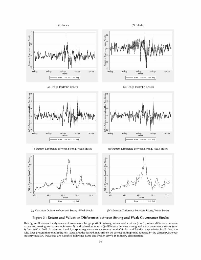
(1) G-Index (2) E-Index

-10

010

20R

etur

ns o

f Gov

erna

nce

Hed

ge P

orfo

lio

90:Sep 94:Sep 98:Sep 02:Sep 06:SepMonth

Raw Ind. Adj.

-15

-10

-50

510

Ret

urns

of G

over

nanc

e H

edge

Por

folio

90:Sep 94:Sep 98:Sep 02:Sep 06:SepMonth

Raw Ind. Adj.

(a) Hedge Portfolio Return (b) Hedge Portfolio Return

-10

-50

510

15D

iff. i

n R

etur

ns b

etw

een

Goo

d/B

ad G

ov. S

tock

s

90:Sep 94:Sep 98:Sep 02:Sep 06:SepMonth

Raw Ind. Adj.

-10

-50

510

15D

iff. i

n R

etur

ns b

etw

een

Goo

d/B

ad G

ov. S

tock

s

90:Sep 94:Sep 98:Sep 02:Sep 06:SepMonth

Raw Ind. Adj.

(c) Return Difference between Strong/Weak Stocks (d) Return Difference between Strong/Weak Stocks

0.5

11.

52

Diff

. in

Q b

etw

een

Goo

d/B

ad G

ov. S

tock

s

90:3 94:3 98:3 02:3 06:3Quarter

Raw Ind. Adj.

0.5

11.

52

Diff

. in

Q b

etw

een

Goo

d/B

ad G

ov. S

tock

s

90:3 94:3 98:3 02:3 06:3Quarter

Raw Ind. Adj.

(e) Valuation Difference between Strong/Weak Stocks (f) Valuation Difference between Strong/Weak Stocks

Figure 3 : Return and Valuation Differences between Strong and Weak Governance Stocks

This figure illustrates the dynamics of governance hedge portfolio (strong minus weak) return (row 1), return difference betweenstrong and weak governance stocks (row 2), and valuation (equity Q) difference between strong and weak governance stocks (row3) from 1990 to 2007. In columns 1 and 2, corporate governance is measured with G-index and E-index, respectively. In all plots, thesolid lines present the series in the raw value, and the dashed lines present the corresponding series adjusted by the contemporaneousindustry median. Industries are classified following Fama and French (1997) 48-industry classification.

39

Table 1 : Summary Statistics of Governance Index and Entrenchment Index

This table describes the summary statistics of governance index (G-Index) and entrenchment index (E-Index) for the years in whichthe data are updated. The data are obtained from RiskMetrics. G-index is constructed following Gompers, Ishii, and Metrick (2003)and E-index is constructed following Bebchuk, Cohen, and Ferrell (2009). S.D., Min, Q1, Q3, Max, and N represent standard devia-tion, minimum, the first and third quartiles, maximum, and the number of companies covered in the volume of the correspondingrespectively.

Year Mean S.D. Min Q1 Median Q3 Max N

A: G-Index1990 8.89 2.89 1 7 9 11 17 1,4671993 9.19 2.88 2 7 9 11 17 1,4631995 9.29 2.81 2 7 9 11 17 1,4961998 8.78 2.85 2 7 9 11 18 1,9132000 8.98 2.69 2 7 9 11 19 1,8872002 9.03 2.64 1 7 9 11 18 1,8942004 9.06 2.55 2 7 9 11 18 1,9822006 9.02 2.52 2 7 9 11 18 1,896Total 9.02 2.72 1 7 9 11 19 13,998

B: E-Index1990 2.14 1.42 0 1 2 3 6 1,4671993 2.23 1.39 0 1 2 3 6 1,4631995 2.23 1.36 0 1 2 3 6 1,4961998 2.19 1.35 0 1 2 3 6 1,9132000 2.35 1.34 0 1 2 3 6 1,8872002 2.39 1.34 0 1 2 3 6 1,8942004 2.45 1.29 0 2 2 3 6 1,9822006 2.43 1.26 0 2 2 3 6 1,896Total 2.31 1.34 0 1 2 3 6 13,998

40

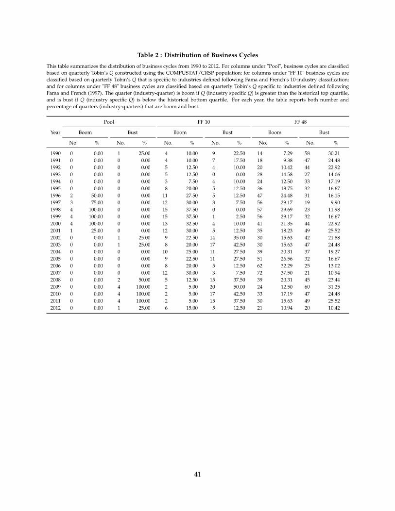
Table 2 : Distribution of Business Cycles

This table summarizes the distribution of business cycles from 1990 to 2012. For columns under "Pool", business cycles are classifiedbased on quarterly Tobin’s Q constructed using the COMPUSTAT/CRSP population; for columns under "FF 10" business cycles areclassified based on quarterly Tobin’s Q that is specific to industries defined following Fama and French’s 10-industry classification;and for columns under "FF 48" business cycles are classified based on quarterly Tobin’s Q specific to industries defined followingFama and French (1997). The quarter (industry-quarter) is boom if Q (industry specific Q) is greater than the historical top quartile,and is bust if Q (industry specific Q) is below the historical bottom quartile. For each year, the table reports both number andpercentage of quarters (industry-quarters) that are boom and bust.

Pool FF 10 FF 48

Year Boom Bust Boom Bust Boom Bust

No. % No. % No. % No. % No. % No. %

1990 0 0.00 1 25.00 4 10.00 9 22.50 14 7.29 58 30.211991 0 0.00 0 0.00 4 10.00 7 17.50 18 9.38 47 24.481992 0 0.00 0 0.00 5 12.50 4 10.00 20 10.42 44 22.921993 0 0.00 0 0.00 5 12.50 0 0.00 28 14.58 27 14.061994 0 0.00 0 0.00 3 7.50 4 10.00 24 12.50 33 17.191995 0 0.00 0 0.00 8 20.00 5 12.50 36 18.75 32 16.671996 2 50.00 0 0.00 11 27.50 5 12.50 47 24.48 31 16.151997 3 75.00 0 0.00 12 30.00 3 7.50 56 29.17 19 9.901998 4 100.00 0 0.00 15 37.50 0 0.00 57 29.69 23 11.981999 4 100.00 0 0.00 15 37.50 1 2.50 56 29.17 32 16.672000 4 100.00 0 0.00 13 32.50 4 10.00 41 21.35 44 22.922001 1 25.00 0 0.00 12 30.00 5 12.50 35 18.23 49 25.522002 0 0.00 1 25.00 9 22.50 14 35.00 30 15.63 42 21.882003 0 0.00 1 25.00 8 20.00 17 42.50 30 15.63 47 24.482004 0 0.00 0 0.00 10 25.00 11 27.50 39 20.31 37 19.272005 0 0.00 0 0.00 9 22.50 11 27.50 51 26.56 32 16.672006 0 0.00 0 0.00 8 20.00 5 12.50 62 32.29 25 13.022007 0 0.00 0 0.00 12 30.00 3 7.50 72 37.50 21 10.942008 0 0.00 2 50.00 5 12.50 15 37.50 39 20.31 45 23.442009 0 0.00 4 100.00 2 5.00 20 50.00 24 12.50 60 31.252010 0 0.00 4 100.00 2 5.00 17 42.50 33 17.19 47 24.482011 0 0.00 4 100.00 2 5.00 15 37.50 30 15.63 49 25.522012 0 0.00 1 25.00 6 15.00 5 12.50 21 10.94 20 10.42

41

Table 3 : Governance, Cycles, Equity Returns, and Valuation – Univariate Analysis

This table summarizes sample means of differences of governance portfolio returns (rGp and rB

p ), single stock returns (rGi and rB

i ),and Tobin’s Q in strong/weak governance portfolios for a sample from 1990 to 2007. Governance portfolio returns are calculatedas the value-weighted average of returns of stocks in the corresponding governance portfolios. Tobin’s Q is defined as the marketcapitalization of a stock divided by the book value of equity. Returns are in monthly frequency and are reported in percentage. Astock is included in the strong governance portfolio if its G(E)-index is smaller than or equal to 5(0), and is included in the weakgovernance portfolio if its G(E)-index is greater than or equal to 14(5). In Panel A, business cycles are classified based on quarterlyTobin’s Q of COMPUSTAT/CRSP population; in Panel B, business cycles are classified based on industry specific Q with industriesclassified in accordance with Fama and French 10-industry classification (FF 10); and in Panel C, business cycles are classified basedon industry specific Q with industries classified in accordance with Fama and French (1997) 48-industry classification (FF 48). Aquarter is boom (bust) if the COMPUSTAT/CRSP (industry-specific) Q is above (below) its historical 80th (20th) percentile. In PanelA, industry-adjusted returns and Q are constructed as their raw value minus the corresponding contemporaneous industry medianwhere industries are classified following Fama and French (1997) 48-industry classification; and in Panel A and B, industry-adjustedreturns and Q are similarly constructed while industries are classified following Fama and French 10-industry and Fama and French(1997) 48-industry classifications, respectively. Superscripts ∗∗∗, ∗∗ , and ∗indicate statistical significance for the two-sided test at0.01, 0.05, and 0.10, respectively. For return differences, the statistic is in bold when the difference is statistically significant at leastat 0.1 level for the one-sided test that the difference is positive (negative) during boom (bust). And for Q differences, the statistic isin bold when the difference is statistically significant at least at 0.1 level for the one-sided test that the difference is positive.

Panel A: Aggregate Business Cycles

G-Index E-Index

Raw Ind. Adj. Raw Ind. Adj.

a. Boom Periods

rGp − rB

p 0.86 1.49∗∗ 1.07 1.36∗∗

rGi − rB

i 0.28 0.45∗ 0.57∗ 0.43

QGi − QB

i 0.81∗∗∗ 0.72∗∗∗ 1.12∗∗∗ 0.87∗∗∗

b. Normal Periods

rGp − rB

p −0.27 −0.32∗ −0.10 −0.11rG

i − rBi 0.11 0.21∗ 0.10 0.25∗

QGi − QB

i 0.42∗∗∗ 0.40∗∗∗ 0.45∗∗∗ 0.35∗∗∗

c. Bust Periods

rGp − rB

p −0.60 −0.26 0.24 0.61rG

i − rBi −1.33∗ −0.64 −0.62 0.17

QGi − QB

i 0.20∗∗∗ 0.19∗∗∗ 0.20∗∗∗ 0.12∗∗∗

Panel B: (FF 10) Industry-Specific Business Cycles

G-Index E-Index

Raw Ind. Adj. Raw Ind. Adj.

a. Boom Periods

rGi − rB

i 0.37 0.54∗ 0.17 0.54∗

QGi − QB

i 1.02∗∗∗ 1.05∗∗∗ 1.43∗∗∗ 1.13∗∗∗

b. Normal Periods

rGi − rB

i 0.05 0.14 0.19 0.26∗QG

i − QBi 0.31∗∗∗ 0.33∗∗∗ 0.34∗∗∗ 0.32∗∗∗

c. Bust Periods

rGi − rB

i −0.50∗ −0.38 −0.23 −0.11QG

i − QBi 0.24∗∗∗ 0.27∗∗∗ −0.02 −0.01

Continued on next page

42

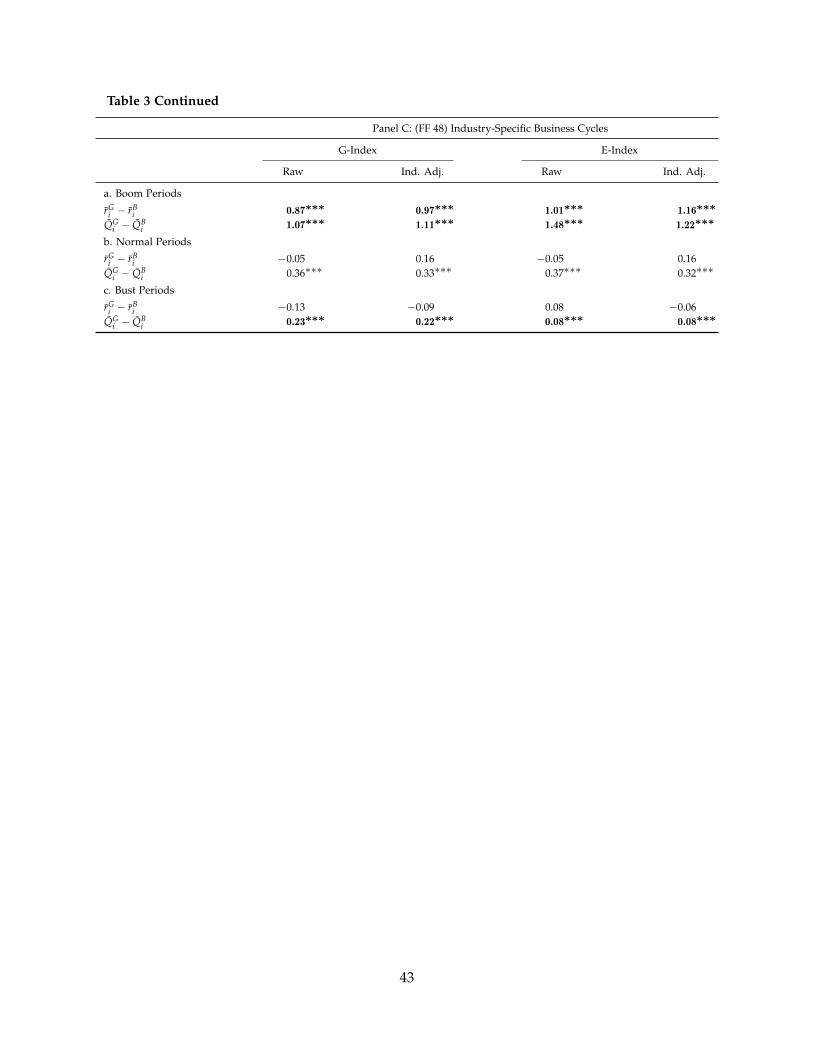
Table 3 Continued

Panel C: (FF 48) Industry-Specific Business Cycles

G-Index E-Index

Raw Ind. Adj. Raw Ind. Adj.

a. Boom Periods

rGi − rB

i 0.87∗∗∗ 0.97∗∗∗ 1.01∗∗∗ 1.16∗∗∗

QGi − QB

i 1.07∗∗∗ 1.11∗∗∗ 1.48∗∗∗ 1.22∗∗∗

b. Normal Periods

rGi − rB

i −0.05 0.16 −0.05 0.16QG

i − QBi 0.36∗∗∗ 0.33∗∗∗ 0.37∗∗∗ 0.32∗∗∗

c. Bust Periods

rGi − rB

i −0.13 −0.09 0.08 −0.06QG

i − QBi 0.23∗∗∗ 0.22∗∗∗ 0.08∗∗∗ 0.08∗∗∗

43

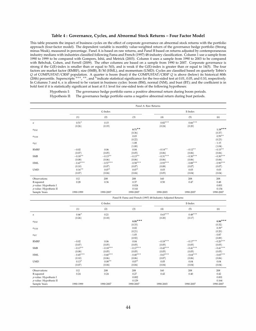
Table 4 : Governance, Cycles, and Abnormal Stock Returns – Four Factor Model

This table presents the impact of business cycles on the effect of corporate governance on abnormal stock returns with the portfolioapproach (four-factor model). The dependent variable is monthly value-weighted return of the governance hedge portfolio (Strongminus Weak), measured in percentage. Panel A is based on raw returns, and Panel B based on returns adjusted by contemporaneousindustry medians with industries classified following Fama and French (1997) 48-industry classification. Column 1 use a sample from1990 to 1999 to be compared with Gompers, Ishii, and Metrick (2003). Column 4 uses a sample from 1990 to 2003 to be comparedwith Bebchuk, Cohen, and Ferrell (2009). The other columns are based on a sample from 1990 to 2007. Corporate governance isstrong if the G(E)-index is smaller than or equal to 5(0), and is weak if the G(E)-index is greater than or equal to 14(5). The fourfactors are market factor (RMRF), size (SMB), B/M (HML), and momentum (UMD). Cycles are classified based on quarterly Tobin’sQ of COMPUSTAT/CRSP population. A quarter is boom (bust) if the COMPUSTAT/CRSP Q is above (below) its historical 80th(20th) percentile. Superscripts ∗∗∗, ∗∗, and ∗indicate statistical significance for the two-sided test at 0.01, 0.05, and 0.10, respectively.In Columns 3 and 6, α is allowed to be variant in business cycles: boom (BM), normal (NM), and bust (BT); and the coefficient is inbold font if it is statistically significant at least at 0.1 level for one-sided tests of the following hypotheses:

Hypothesis I: The governance hedge portfolio earns a positive abnormal return during boom periods.Hypothesis II: The governance hedge portfolio earns a negative abnormal return during bust periods.

Panel A: Raw Returns

G-Index E-Index

(1) (2) (3) (4) (5) (6)

α 0.51∗ 0.15 0.82∗∗∗ 0.66∗∗∗(0.26) (0.19) (0.24) (0.20)

αBM 0.71∗∗ 1.19∗∗∗

(0.36) (0.37)αNM 0.03 0.59∗∗

(0.22) (0.23)αBT −1.08 −1.15

(1.00) (1.04)RMRF −0.02 0.06 0.04 −0.14∗∗ −0.12∗∗ −0.15∗∗

(0.07) (0.05) (0.05) (0.06) (0.06) (0.06)SMB −0.18∗∗ −0.13∗∗ −0.13∗∗ −0.31∗∗∗ −0.30∗∗∗ −0.30∗∗∗

(0.08) (0.06) (0.06) (0.06) (0.06) (0.06)HML −0.47∗∗∗ −0.57∗∗∗ −0.58∗∗∗ −0.93∗∗∗ −0.88∗∗∗ −0.90∗∗∗

(0.10) (0.07) (0.07) (0.08) (0.07) (0.07)UMD 0.16∗∗ 0.07∗ 0.07∗ 0.03 0.03 0.03

(0.07) (0.04) (0.04) (0.05) (0.04) (0.04)

Observations 112 208 208 160 208 208R-squared 0.28 0.36 0.37 0.50 0.47 0.48p-value: Hypothesis I 0.024 0.001p-value: Hypothesis II 0.141 0.134Sample Years 1990-1999 1990-2007 1990-2007 1990-2003 1990-2007 1990-2007

Panel B: Fama and French (1997) 48-Industry-Adjusted Returns

G-Index E-Index

(1) (2) (3) (4) (5) (6)

α 0.46∗ 0.21 0.63∗∗∗ 0.48∗∗∗(0.26) (0.18) (0.20) (0.17)

αBM 0.95∗∗∗ 0.96∗∗∗

(0.33) (0.32)αNM 0.02 0.39∗

(0.21) (0.20)αBT −1.05 −0.87

(0.92) (0.89)RMRF −0.02 0.06 0.04 −0.18∗∗∗ −0.17∗∗∗ −0.20∗∗∗

(0.07) (0.05) (0.05) (0.05) (0.05) (0.05)SMB −0.17∗∗ −0.18∗∗∗ −0.17∗∗∗ −0.42∗∗∗ −0.41∗∗∗ −0.41∗∗∗

(0.08) (0.05) (0.05) (0.05) (0.05) (0.05)HML −0.45∗∗∗ −0.40∗∗∗ −0.40∗∗∗ −0.67∗∗∗ −0.64∗∗∗ −0.65∗∗∗

(0.10) (0.06) (0.06) (0.07) (0.06) (0.06)UMD 0.13∗ 0.08∗∗ 0.07∗ 0.05 0.04 0.04

(0.07) (0.04) (0.04) (0.04) (0.04) (0.04)

Observations 112 208 208 160 208 208R-squared 0.24 0.24 0.27 0.42 0.40 0.42p-value: Hypothesis I 0.002 0.001p-value: Hypothesis II 0.129 0.164Sample Years 1990-1999 1990-2007 1990-2007 1990-2003 1990-2007 1990-2007

44

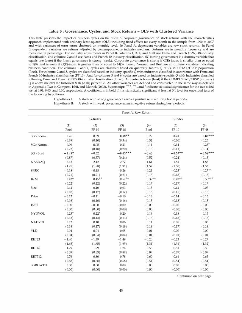
Table 5 : Governance, Cycles, and Stock Returns – OLS with Clustered Variance

This table presents the impact of business cycles on the effect of corporate governance on stock returns with the characteristicsapproach implemented with ordinary least squares (OLS) including fixed effects for every month in the sample from 1990 to 2007and with variances of error terms clustered on monthly level. In Panel A, dependent variables are raw stock returns. In PanelB, dependent variables are returns adjusted by contemporaneous industry medians. Returns are in monthly frequency and aremeasured in percentage. For industry adjustments in Panel B, columns 1, 3, 4, and 6 all use Fama and French (1997) 48-industryclassification, and columns 2 and 5 use Fama and French 10-industry classification. SG (strong governance) is a dummy variable thatequals one (zero) if the firm’s governance is strong (weak). Corporate governance is strong if G(E)-index is smaller than or equalto 5(0), and is weak if G(E)-index is greater than or equal to 14(5). Boom, Normal, and Bust are all dummy variables indicatingbusiness condition. For columns 1 and 4, cycles are classified based on quarterly Tobin’s Q of COMPUSTAT/CRSP population(Pool). For columns 2 and 5, cycles are classified based on industry specific Q with industries classified in accordance with Fama andFrench 10-industry classification (FF 10). And for columns 3 and 6, cycles are based on industry-specific Q with industries classifiedfollowing Fama and French (1997) 48-industry classification (FF 48). A quarter is boom (bust) if the COMPUSTAT/CRSP (industry)Q is above (below) the historical 80th (20th) percentile. All other variables are defined and constructed in the same way as detailedin Appendix Two in Gompers, Ishii, and Metrick (2003). Superscripts ∗∗∗, ∗∗, and ∗indicate statistical significance for the two-sidedtest at 0.01, 0.05, and 0.10, respectively. A coefficient is in bold if it is statistically significant at least at 0.1 level for one-sided tests ofthe following hypotheses:

Hypothesis I: A stock with strong governance earns a positive return during boom periods.Hypothesis II: A stock with weak governance earns a negative return during bust periods.

Panel A: Raw Return

G-Index E-Index

(1) (2) (3) (4) (5) (6)Pool FF 10 FF 48 Pool FF 10 FF 48

SG×Boom 0.26 0.39 0.69∗∗ 0.29 0.45 0.66∗∗∗

(0.39) (0.40) (0.34) (0.32) (0.30) (0.25)SG×Normal 0.09 0.05 0.21 0.11 0.14 0.23∗

(0.22) (0.18) (0.20) (0.13) (0.11) (0.14)SG×Bust −1.49∗ −0.32 −0.63∗∗∗ −0.46 −0.57∗∗ −0.58∗∗∗

(0.87) (0.37) (0.24) (0.52) (0.24) (0.15)NASDAQ 2.13 2.42 2.77 1.64 1.81 1.85

(1.95) (1.88) (1.91) (1.57) (1.50) (1.53)SP500 −0.18 −0.18 −0.26 −0.21 −0.23∗ −0.27∗∗

(0.21) (0.21) (0.21) (0.13) (0.13) (0.13)B/M 0.42∗ 0.45∗∗ 0.52∗∗ 0.39∗∗ 0.43∗∗ 0.50∗∗∗

(0.22) (0.22) (0.22) (0.17) (0.17) (0.17)Size −0.12 −0.10 −0.03 −0.15 −0.12 −0.07

(0.18) (0.17) (0.17) (0.16) (0.15) (0.15)Price −0.12 −0.11 −0.10 −0.16 −0.14 −0.15

(0.16) (0.16) (0.16) (0.13) (0.13) (0.13)INST −0.00 −0.00 −0.00 −0.00 −0.00 −0.00

(0.00) (0.00) (0.00) (0.00) (0.00) (0.00)NYDVOL 0.23∗ 0.22∗ 0.20 0.19 0.18 0.15

(0.13) (0.13) (0.13) (0.13) (0.13) (0.13)NADVOL 0.12 0.10 0.06 0.11 0.08 0.06

(0.18) (0.17) (0.18) (0.18) (0.17) (0.18)YLD 0.04 0.04 0.05 −0.01 −0.00 −0.00

(0.04) (0.04) (0.04) (0.01) (0.01) (0.01)RET23 −1.40 −1.39 −1.49 −0.20 −0.23 −0.27

(1.65) (1.65) (1.65) (1.31) (1.31) (1.32)RET46 1.29 1.29 1.24 0.53 0.51 0.50

(0.89) (0.89) (0.89) (0.89) (0.89) (0.89)RET712 0.76 0.80 0.78 0.60 0.61 0.63

(0.68) (0.68) (0.68) (0.54) (0.54) (0.54)SGROWTH 0.00 0.00 0.00 0.00 0.00 0.00

(0.00) (0.00) (0.00) (0.00) (0.00) (0.00)

Continued on next page

45

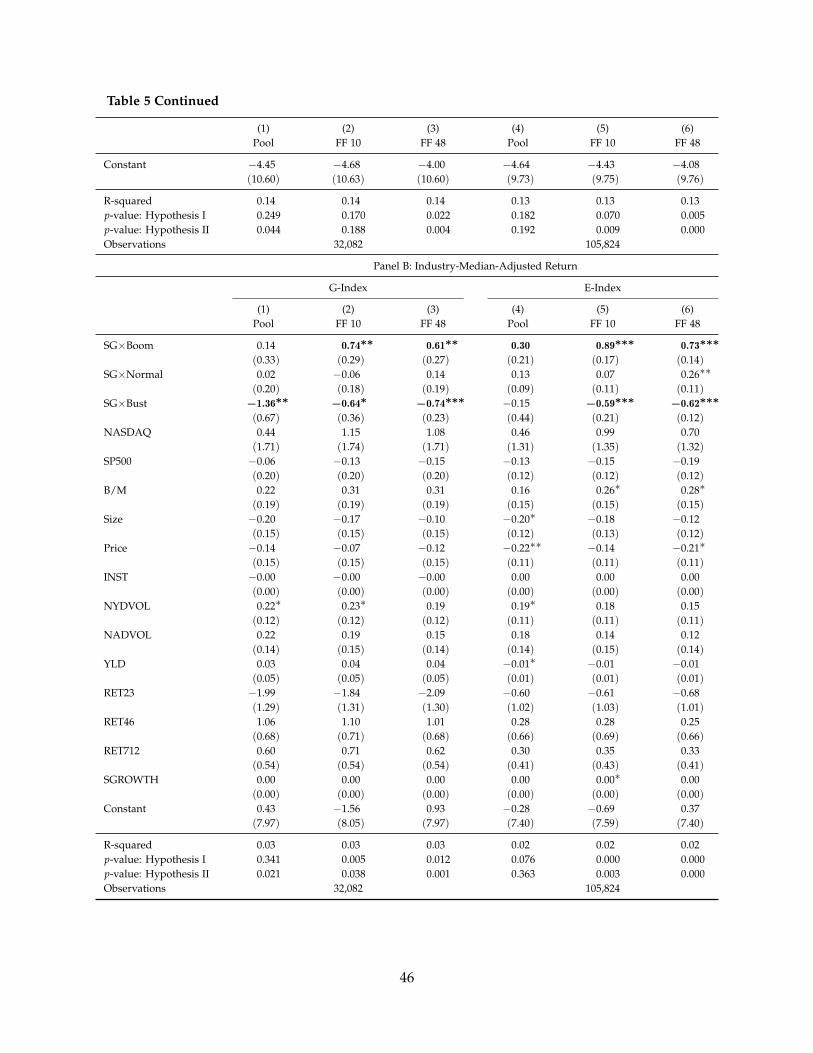
Table 5 Continued

(1) (2) (3) (4) (5) (6)Pool FF 10 FF 48 Pool FF 10 FF 48

Constant −4.45 −4.68 −4.00 −4.64 −4.43 −4.08(10.60) (10.63) (10.60) (9.73) (9.75) (9.76)

R-squared 0.14 0.14 0.14 0.13 0.13 0.13p-value: Hypothesis I 0.249 0.170 0.022 0.182 0.070 0.005p-value: Hypothesis II 0.044 0.188 0.004 0.192 0.009 0.000Observations 32,082 105,824

Panel B: Industry-Median-Adjusted Return

G-Index E-Index

(1) (2) (3) (4) (5) (6)Pool FF 10 FF 48 Pool FF 10 FF 48

SG×Boom 0.14 0.74∗∗ 0.61∗∗ 0.30 0.89∗∗∗ 0.73∗∗∗

(0.33) (0.29) (0.27) (0.21) (0.17) (0.14)SG×Normal 0.02 −0.06 0.14 0.13 0.07 0.26∗∗

(0.20) (0.18) (0.19) (0.09) (0.11) (0.11)SG×Bust −1.36∗∗ −0.64∗ −0.74∗∗∗ −0.15 −0.59∗∗∗ −0.62∗∗∗

(0.67) (0.36) (0.23) (0.44) (0.21) (0.12)NASDAQ 0.44 1.15 1.08 0.46 0.99 0.70

(1.71) (1.74) (1.71) (1.31) (1.35) (1.32)SP500 −0.06 −0.13 −0.15 −0.13 −0.15 −0.19

(0.20) (0.20) (0.20) (0.12) (0.12) (0.12)B/M 0.22 0.31 0.31 0.16 0.26∗ 0.28∗

(0.19) (0.19) (0.19) (0.15) (0.15) (0.15)Size −0.20 −0.17 −0.10 −0.20∗ −0.18 −0.12

(0.15) (0.15) (0.15) (0.12) (0.13) (0.12)Price −0.14 −0.07 −0.12 −0.22∗∗ −0.14 −0.21∗

(0.15) (0.15) (0.15) (0.11) (0.11) (0.11)INST −0.00 −0.00 −0.00 0.00 0.00 0.00

(0.00) (0.00) (0.00) (0.00) (0.00) (0.00)NYDVOL 0.22∗ 0.23∗ 0.19 0.19∗ 0.18 0.15

(0.12) (0.12) (0.12) (0.11) (0.11) (0.11)NADVOL 0.22 0.19 0.15 0.18 0.14 0.12

(0.14) (0.15) (0.14) (0.14) (0.15) (0.14)YLD 0.03 0.04 0.04 −0.01∗ −0.01 −0.01

(0.05) (0.05) (0.05) (0.01) (0.01) (0.01)RET23 −1.99 −1.84 −2.09 −0.60 −0.61 −0.68

(1.29) (1.31) (1.30) (1.02) (1.03) (1.01)RET46 1.06 1.10 1.01 0.28 0.28 0.25

(0.68) (0.71) (0.68) (0.66) (0.69) (0.66)RET712 0.60 0.71 0.62 0.30 0.35 0.33

(0.54) (0.54) (0.54) (0.41) (0.43) (0.41)SGROWTH 0.00 0.00 0.00 0.00 0.00∗ 0.00

(0.00) (0.00) (0.00) (0.00) (0.00) (0.00)Constant 0.43 −1.56 0.93 −0.28 −0.69 0.37

(7.97) (8.05) (7.97) (7.40) (7.59) (7.40)

R-squared 0.03 0.03 0.03 0.02 0.02 0.02p-value: Hypothesis I 0.341 0.005 0.012 0.076 0.000 0.000p-value: Hypothesis II 0.021 0.038 0.001 0.363 0.003 0.000Observations 32,082 105,824

46

Table 6 : Governance, Cycles, and Stock Returns – Fama and MacBeth (1973)

This table presents the impact of business cycles on the effect of corporate governance on stock returns with the characteristicsapproach implemented with Fama and MacBeth (1973) method using a sample from 1990 to 2007. In Panel A, dependent variablesare raw stock returns. In Panel B, dependent variables are returns adjusted by contemporaneous industry medians. Returns are inmonthly frequency and are measured in percentage. For industry adjustments in Panel B, columns 1, and 3 use Fama and French10-industry classification, and columns 2 and 4 use Fama and French (1997) 48-industry classification. SG (strong governance) is adummy variable that equals one (zero) if the firm’s governance is strong (weak). Corporate governance is strong if G(E)-index issmaller than or equal to 5(0), and is weak if G(E)-index is greater than or equal to 14(5). Boom, Normal, and Bust are all dummyvariables indicating business condition. Cycles are based on industry specific Q. Columns 1 and 3 use Fama and French 10-industryclassification (FF 10) and columns 2 and 4 use Fama and French (1997) 48-industry classification (FF 48). A quarter is boom (bust)if the industry Q is above (below) the historical 80th (20th) percentile. All other variables are defined and constructed in the sameway as detailed in Appendix Two in Gompers, Ishii, and Metrick (2003). Superscripts ∗∗∗ , ∗∗ , and ∗indicate statistical significancefor the two-sided test at 0.01, 0.05, and 0.10, respectively. A coefficient is in bold if it is statistically significant at least at 0.1 level forone-sided tests of the following hypotheses:

Hypothesis I: A stock with strong governance earns a positive return during boom periods.Hypothesis II: A stock with weak governance earns a negative return during bust periods.

Panel A: Raw Return

G-Index E-Index

(1) (2) (3) (4)FF 10 FF 48 FF 10 FF 48

SG×Boom 0.51 0.65 0.56∗∗ 0.60∗∗∗

(0.44) (0.44) (0.25) (0.21)SG×Normal −0.05 0.18 0.01 0.18

(0.16) (0.18) (0.09) (0.11)SG×Bust −0.42 −0.40∗ −0.57∗∗ −0.44∗∗∗

(0.25) (0.24) (0.26) (0.13)NASDAQ −0.15 0.27 −0.32 −0.15

(1.95) (1.94) (1.26) (1.26)SP500 −0.09 −0.14 −0.20 −0.22∗

(0.20) (0.20) (0.12) (0.12)B/M 0.27∗ 0.30∗∗ 0.29∗∗∗ 0.31∗∗∗

(0.14) (0.14) (0.09) (0.09)Size −0.07 −0.02 −0.03 0.01

(0.16) (0.16) (0.12) (0.12)Price 0.03 0.03 −0.10 −0.10

(0.13) (0.13) (0.11) (0.11)INST 0.00 0.00 −0.00 −0.00

(0.00) (0.00) (0.00) (0.00)NYDVOL 0.09 0.09 0.06 0.03

(0.11) (0.11) (0.09) (0.10)NADVOL 0.12 0.09 0.09 0.05

(0.14) (0.15) (0.13) (0.13)YLD −0.03 −0.03 −0.03 −0.03

(0.04) (0.04) (0.02) (0.02)RET23 0.47 0.35 0.61 0.67

(0.80) (0.81) (0.59) (0.60)RET46 1.61∗∗∗ 1.57∗∗∗ 0.97∗∗ 1.03∗∗

(0.59) (0.60) (0.45) (0.45)RET712 1.28∗∗∗ 1.18∗∗∗ 1.02∗∗∗ 1.03∗∗∗

(0.42) (0.43) (0.33) (0.33)SGROWTH 0.00 0.00 −0.00 −0.00

(0.00) (0.00) (0.00) (0.00)Constant −15.66∗∗∗ −14.54∗∗ −11.03∗∗ −11.46∗∗

(5.95) (5.98) (4.82) (4.84)

Continued on next page

47

Table 6 Continued

(1) (2) (3) (4)FF 10 FF 48 FF 10 FF 48

R-squared 0.21 0.22 0.13 0.13p-value: Hypothesis I 0.124 0.067 0.014 0.002p-value: Hypothesis II 0.051 0.047 0.014 0.000Observations 32,082 105,824Number of Months 208

Panel B: Industry-Median-Adjusted Return

G-Index E-Index

(1) (2) (3) (4)FF 10 FF 48 FF 10 FF 48

SG×Boom 0.69∗ 0.66 0.88∗∗∗ 0.65∗∗∗

(0.41) (0.42) (0.19) (0.16)SG×Normal −0.16 0.04 −0.06 0.19∗

(0.17) (0.18) (0.10) (0.10)SG×Bust −0.51∗ −0.50∗∗ −0.33 −0.50∗∗∗

(0.27) (0.24) (0.21) (0.12)NASDAQ −0.39 −0.40 −0.18 −0.26

(1.88) (1.82) (1.20) (1.19)SP500 0.02 0.06 −0.11 −0.13

(0.20) (0.20) (0.12) (0.12)B/M 0.17 0.15 0.16∗ 0.13

(0.14) (0.14) (0.09) (0.09)Size −0.12 −0.10 −0.07 −0.04

(0.15) (0.15) (0.11) (0.11)Price 0.03 0.00 −0.11 −0.17∗

(0.13) (0.13) (0.10) (0.10)INST 0.00 −0.00 0.00 0.00

(0.00) (0.00) (0.00) (0.00)NYDVOL 0.08 0.08 0.05 0.03

(0.11) (0.11) (0.09) (0.09)NADVOL 0.13 0.12 0.07 0.06

(0.14) (0.13) (0.12) (0.11)YLD −0.07∗ −0.08∗∗ −0.04∗∗ −0.04∗∗∗

(0.04) (0.04) (0.02) (0.02)RET23 0.44 −0.04 0.48 0.41

(0.78) (0.76) (0.56) (0.55)RET46 1.62∗∗∗ 1.44∗∗ 0.90∗∗ 0.84∗∗

(0.56) (0.55) (0.41) (0.40)RET712 1.08∗∗∗ 0.95∗∗ 0.77∗∗ 0.74∗∗

(0.41) (0.39) (0.31) (0.30)SGROWTH 0.00 0.00 −0.00 −0.00

(0.00) (0.00) (0.00) (0.00)Constant −14.47∗∗ −10.47∗ −9.08∗∗ −7.95∗

(5.59) (5.42) (4.40) (4.25)

R-squared 0.19 0.19 0.10 0.10p-value: Hypothesis I 0.047 0.057 0.000 0.000p-value: Hypothesis II 0.029 0.022 0.059 0.000Observations 32,082 105,824Number of Months 208

48

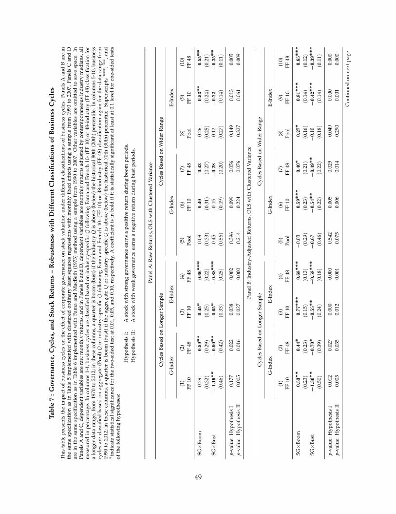
Tabl

e7

:Gov

erna

nce,

Cyc

les,

and

Stoc

kR

etur

ns–

Rob

ustn

ess

wit

hD

iffe

rent

Cla

ssifi

cati

ons

ofB

usin

ess

Cyc

les

This

tabl

epr

esen

tsth

eim

pact

ofbu

sine

sscy

cles

onth

eef

fect

ofco

rpor

ate

gove

rnan

ceon

stoc

kva

luat

ion

unde

rdi

ffer

ent

clas

sific

atio

nsof

busi

ness

cycl

es.

Pane

lsA

and

Bar

ein

the

sam

esp

ecifi

cati

onas

inTa

ble

5im

plem

ente

dw

ith

clus

tere

dor

dina

ryle

ast

squa

res

regr

essi

ons

wit

hm

onth

lyfix

edef

fect

sus

ing

asa

mpl

efr

om19

90to

2007

,Pan

els

Can

dD

are

inth

esa

me

spec

ifica

tion

asin

Tabl

e6

impl

emen

ted

wit

hFa

ma

and

Mac

Beth

(197

3)m

etho

dus

ing

asa

mpl

efr

om19

90to

2007

.O

ther

vari

able

sar

eom

itte

dto

save

spac

e.In

Pane

lsA

and

C,d

epen

dent

vari

able

sar

era

wm

onth

lyre

turn

s,an

din

Pane

lsB

and

D,d

epen

dent

vari

able

sar

em

onth

lyre

turn

sad

just

edby

cont

empo

rane

ous

indu

stry

med

ians

,all

mea

sure

din

perc

enta

ge.

Inco

lum

ns1-

4,bu

sine

sscy

cles

are

clas

sifie

dba

sed

onin

dust

ry-s

peci

ficQ

follo

win

gFa

ma

and

Fren

ch10

-(F

F10

)or

48-i

ndus

try

(FF

48)

clas

sific

atio

nfo

ra

long

erda

tara

nge,

from

1970

to20

12;i

nth

ese

colu

mns

,aqu

arte

ris

boom

(bus

t)if

the

indu

stry

Qis

abov

e(b

elow

)th

ehi

stor

ical

80th

(20t

h)pe

rcen

tile

.In

colu

mns

5-10

,bus

ines

scy

cles

are

clas

sifie

dba

sed

onag

greg

ate

(Poo

l)Q

orin

dust

ry-s

peci

ficQ

follo

win

gFa

ma

and

Fren

ch10

-(F

F10

)or

48-i

ndus

try

(FF

48)

clas

sific

atio

nag

ain

for

the

data

rang

efr

om19

90to

2012

;in

thes

eco

lum

ns,a

quar

ter

isbo

om(b

ust)

ifth

eag

greg

ate

Qor

indu

stry

-spe

cific

Qis

abov

e(b

elow

)th

ehi

stor

ical

70th

(30t

h)pe

rcen

tile

.Su

pers

crip

ts∗∗∗ ,∗∗

,and

∗ ind

icat

est

atis

tica

lsig

nific

ance

for

the

two-

side

dte

stat

0.01

,0.0

5,an

d0.

10,r

espe

ctiv

ely.

Aco

effic

ient

isin

bold

ifit

isst

atis

tica

llysi

gnifi

cant

atle

asta

t0.1

leve

lfor

one-

side

dte

sts

ofth

efo

llow

ing

hypo

thes

es:

Hyp

othe

sis

I:A

stoc

kw

ith

stro

nggo

vern

ance

earn

sa

posi

tive

retu

rndu

ring

boom

peri

ods.

Hyp

othe

sis

II:

Ast

ock

wit

hw

eak

gove

rnan

ceea

rns

ane

gati

vere

turn

duri

ngbu

stpe

riod

s.

Pane

lA:R

awR

etur

ns,O

LSw

ith

Clu

ster

edV

aria

nce

Cyc

les

Base

don

Long

erSa

mpl

eC

ycle

sBa

sed

onW

ider

Ran

ge

G-I

ndex

E-In

dex

G-I

ndex

E-In

dex

(1)

(2)

(3)

(4)

(5)

(6)

(7)

(8)

(9)

(10)

FF10

FF48

FF10

FF48

Pool

FF10

FF48

Pool

FF10

FF48

SG×

Boom

0.29

0.59∗∗

0.45

∗0.66∗∗

∗0.

090.40

0.43

0.26

0.53∗

∗0.55∗

∗

(0.3

2)(0

.29)

(0.2

5)(0

.22)

(0.3

3)(0

.31)

(0.2

7)(0

.25)

(0.2

4)(0

.21)

SG×

Bust

−1.19∗

∗−0.90∗

∗−0.65∗

−0.88∗∗

∗−

0.45

−0.

15−0.28

−0.

12−0.22

−0.25∗

∗

(0.4

6)(0

.42)

(0.3

3)(0

.25)

(0.5

6)(0

.19)

(0.2

0)(0

.27)

(0.1

4)(0

.11)

p-va

lue:

Hyp

othe

sis

I0.

177

0.02

20.

038

0.00

20.

396

0.09

90.

056

0.14

90.

013

0.00

5p-

valu

e:H

ypot

hesi

sII

0.00

50.

016

0.02

70.

000

0.21

40.

224

0.07

60.

327

0.06

10.

009

Pane

lB:I

ndus

try-

Adj

uste

dR

etur

ns,O

LSw

ith

Clu

ster

edV

aria

nce

Cyc

les

Base

don

Long

erSa

mpl

eC

ycle

sBa

sed

onW

ider

Ran

ge

G-I

ndex

E-In

dex

G-I

ndex

E-In

dex

(1)

(2)

(3)

(4)

(5)

(6)

(7)

(8)

(9)

(10)

FF10

FF48

FF10

FF48

Pool

FF10

FF48

Pool

FF10

FF48

SG×

Boom

0.53∗∗

0.44∗

0.77

∗∗∗

0.68∗∗

∗−

0.03

0.59∗∗

∗0.40∗

0.27∗

0.81∗

∗∗0.65∗

∗∗

(0.2

3)(0

.23)

(0.1

5)(0

.13)

(0.2

9)(0

.23)

(0.2

1)(0

.16)

(0.1

4)(0

.12)

SG×

Bust

−1.30∗

∗−0.70∗

−0.55∗∗

−0.58∗∗

∗−0.67

−0.54∗∗

−0.49∗

∗−

0.10

−0.42∗

∗∗−0.39∗

∗∗

(0.5

0)(0

.39)

(0.2

4)(0

.18)

(0.4

6)(0

.22)

(0.2

2)(0

.18)

(0.1

4)(0

.11)

p-va

lue:

Hyp

othe

sis

I0.

012

0.02

70.

000

0.00

00.

542

0.00

50.

029

0.04

90.

000

0.00

0p-

valu

e:H

ypot

hesi

sII

0.00

50.

035

0.01

20.

001

0.07

50.

006

0.01

40.

290

0.00

10.

000

Con

tinu

edon

next

page

49

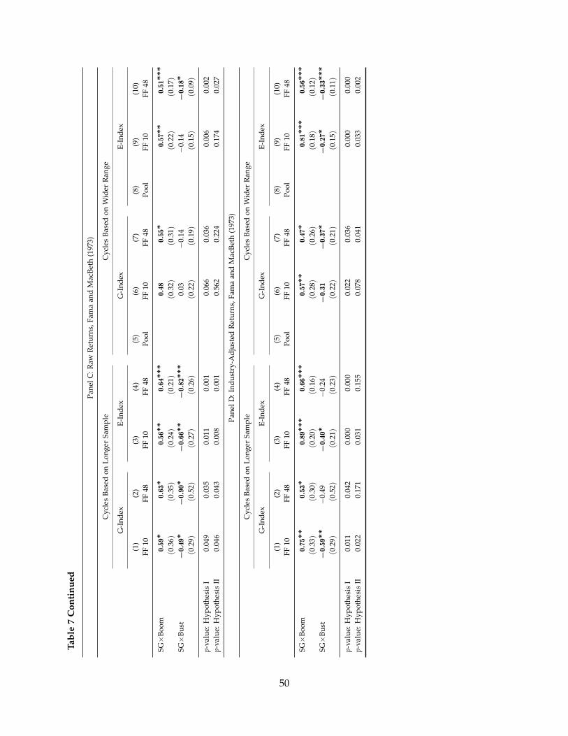
Tabl

e7

Con

tinu

ed

Pane

lC:R

awR

etur

ns,F

ama

and

Mac

Beth

(197

3)

Cyc

les

Base

don

Long

erSa

mpl

eC

ycle

sBa

sed

onW

ider

Ran

ge

G-I

ndex

E-In

dex

G-I

ndex

E-In

dex

(1)

(2)

(3)

(4)

(5)

(6)

(7)

(8)

(9)

(10)

FF10

FF48

FF10

FF48

Pool

FF10

FF48

Pool

FF10

FF48

SG×

Boom

0.59∗

0.63∗

0.56∗∗

0.64∗∗

∗0.48

0.55∗

0.57∗

∗0.51∗

∗∗

(0.3

6)(0

.35)

(0.2

4)(0

.21)

(0.3

2)(0

.31)

(0.2

2)(0

.17)

SG×

Bust

−0.49∗

−0.90∗

−0.66∗∗

−0.82∗∗

∗0.

03−

0.14

−0.

14−0.18∗

(0.2

9)(0

.52)

(0.2

7)(0

.26)

(0.2

2)(0

.19)

(0.1

5)(0

.09)

p-va

lue:

Hyp

othe

sis

I0.

049

0.03

50.

011

0.00

10.

066

0.03

60.

006

0.00

2p-

valu

e:H

ypot

hesi

sII

0.04

60.

043

0.00

80.

001

0.56

20.

224

0.17

40.

027

Pane

lD:I

ndus

try-

Adj

uste

dR

etur

ns,F

ama

and

Mac

Beth

(197

3)

Cyc

les

Base

don

Long

erSa

mpl

eC

ycle

sBa

sed

onW

ider

Ran

ge

G-I

ndex

E-In

dex

G-I

ndex

E-In

dex

(1)

(2)

(3)

(4)

(5)

(6)

(7)

(8)

(9)

(10)

FF10

FF48

FF10

FF48

Pool

FF10

FF48

Pool

FF10

FF48

SG×

Boom

0.75∗

∗0.53∗

0.89∗∗

∗0.66∗∗

∗0.57∗∗

0.47∗

0.81∗

∗∗0.56∗

∗∗

(0.3

3)(0

.30)

(0.2

0)(0

.16)

(0.2

8)(0

.26)

(0.1

8)(0

.12)

SG×

Bust

−0.59∗

∗−

0.49

−0.40∗

−0.

24−0.31

−0.37∗

−0.27∗

−0.33∗

∗∗

(0.2

9)(0

.52)

(0.2

1)(0

.23)

(0.2

2)(0

.21)

(0.1

5)(0

.11)

p-va

lue:

Hyp

othe

sis

I0.

011

0.04

20.

000

0.00

00.

022

0.03

60.

000

0.00

0p-

valu

e:H

ypot

hesi

sII

0.02

20.

171

0.03

10.

155

0.07

80.

041

0.03

30.

002

50

Table 8 : Governance, Cycles, and Stock Returns – Robustness with Alternative Governance Measure

This table presents robustness of procyclicality of corporate governance’s effect on stock returns with corporate governance mea-sured with product market competition. The dependent variables are either monthly stock returns (columns 1 and 3) or monthlyindustry-adjusted stock returns (columns 2 and 4), measured in percentage. Product market competition is measured by Herfindahl-Hirschman (Herfindah, 1950; Hirschman, 1945) Index of the industry in which the firm is operating, or HHI. HHI is calculated usingsales of the companies in the industry. SG (strong governance) is a dummy variable that equals one (zero) if the firm’s governanceis strong (weak). Corporate governance is strong (weak) if the company is in a competitive (concentrated) industry. An industryis competitive (concentrated) if is HHI is below (above) the contemporaneous bottom (top) quartile. Boom and Bust are dummyvariables indicating business condition. Cycles are based on industry specific Q. A quarter is boom (bust) if the industry Q is above(below) the historical 80th (20th) percentile. In Panel A, business cycles are classified using a sample of industry Tobin’s Q from 1990to 2012; in Panel B, business cycles are classified using a longer sample of industry Q from 1970 to 2012. In This table, industriesare classified using Fama and French (1997) 48-industry definition. Regression specification is the same as in Tables 5 and 6. Othervariables are omitted to save space. Superscripts ∗∗∗, ∗∗ , and ∗indicate statistical significance for the two-sided test at 0.01, 0.05,and 0.10, respectively. A coefficient is in bold if it is statistically significant at least at 0.1 level for one-sided tests of the followinghypotheses:

Hypothesis I: A stock with strong governance earns a positive return during boom periods.Hypothesis II: A stock with weak governance earns a negative return during bust periods.

Panel A: Cycles in 1990-2012

Clustered OLS Fama and MacBeth (1973)

(1) (2) (3) (4)Raw Ind. Adj. Raw Ind. Adj.

SG×Boom 0.33∗∗ 0.34∗∗∗ 0.28 0.41∗∗

(0.15) (0.10) (0.19) (0.17)SG×Bust −0.53∗∗∗ −0.66∗∗∗ −0.34∗∗∗ −0.60∗∗∗

(0.16) (0.10) (0.15) (0.10)

p-value: Hypothesis I 0.015 0.001 0.071 0.010p-value: Hypothesis II 0.000 0.000 0.011 0.000Sample Years 1990-2011

Panel B: Cycles in 1970-2012

Clustered OLS Fama and MacBeth (1973)

(1) (2) (3) (4)Raw Ind. Adj. Raw Ind. Adj.

SG×Boom 0.48∗∗∗ 0.27∗∗∗ 0.38∗∗∗ 0.22∗∗

(0.14) (0.08) (0.12) (0.11)SG×Bust −0.74∗∗∗ −0.58∗∗∗ −0.62∗∗∗ −0.41∗∗∗

(0.21) (0.08) (0.13) (0.09)

p-value: Hypothesis I 0.000 0.000 0.001 0.023p-value: Hypothesis II 0.000 0.000 0.000 0.000Sample Years 1975-2011

51

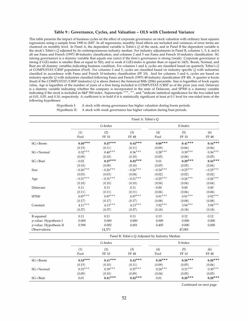
Table 9 : Governance, Cycles, and Valuation – OLS with Clustered Variance

This table presents the impact of business cycles on the effect of corporate governance on stock valuation with ordinary least squaresregressions using a sample from 1990 to 2007. In all regressions, monthly fixed effects are included and variances of error terms areclustered on monthly level. In Panel A, the dependent variable is Tobin’s Q of the stock, and in Panel B the dependent variable isthe stock’s Tobin’s Q adjusted by its contemporaneous industry median. For industry adjustments in Panel B, columns 1, 3, 4, and 6all use Fama and French (1997) 48-industry classification, and columns 2 and 5 use Fama and French 10-industry classification. SG(strong governance) is a dummy variable that equals one (zero) if the firm’s governance is strong (weak). Corporate governance isstrong if G(E)-index is smaller than or equal to 5(0), and is weak if G(E)-index is greater than or equal to 14(5). Boom, Normal, andBust are all dummy variables indicating business condition. For columns 1 and 4, cycles are classified based on quarterly Tobin’s Qof COMPUSTAT/CRSP population (Pool). For columns 2 and 5, cycles are classified based on industry specific Q with industriesclassified in accordance with Fama and French 10-industry classification (FF 10). And for columns 3 and 6, cycles are based onindustry-specific Q with industries classified following Fama and French (1997) 48-industry classification (FF 48). A quarter is boom(bust) if the COMPUSTAT/CRSP (industry) Q is above (below) the historical 80th (20th) percentile. Size is logarithm of book equityvalue, Age is logarithm of the number of years of a firm being included in COMPUSTAT/CRSP as of the prior year end, Delawareis a dummy variable indicating whether the company is incorporated in the state of Delaware, and SP500 is a dummy variableindicating if the stock is included in S&P 500 index. Superscripts ∗∗∗, ∗∗ , and ∗indicate statistical significance for the two-sided testat 0.01, 0.05, and 0.10, respectively. A coefficient is in bold if it is statistically significant at least at 0.1 level for one-sided tests of thefollowing hypotheses:

Hypothesis I: A stock with strong governance has higher valuation during boom periods.Hypothesis II: A stock with weak governance has higher valuation during bust periods.

Panel A: Tobin’s Q

G-Index E-Index

(1) (2) (3) (4) (5) (6)Pool FF 10 FF 48 Pool FF 10 FF 48

SG×Boom 0.56∗∗∗ 0.37∗∗∗ 0.43∗∗∗ 0.68∗∗∗ 0.41∗∗∗ 0.44∗∗∗

(0.15) (0.11) (0.11) (0.09) (0.06) (0.06)SG×Normal 0.32∗∗∗ 0.40∗∗∗ 0.36∗∗∗ 0.28∗∗∗ 0.39∗∗∗ 0.36∗∗∗

(0.09) (0.10) (0.10) (0.05) (0.06) (0.05)SG×Bust −0.02 0.27∗∗∗ 0.32∗∗∗ 0.01 0.29∗∗∗ 0.34∗∗∗

(0.10) (0.09) (0.10) (0.05) (0.05) (0.06)Size −0.26∗∗∗ −0.26∗∗∗ −0.26∗∗∗ −0.24∗∗∗ −0.25∗∗∗ −0.25∗∗∗

(0.03) (0.03) (0.04) (0.02) (0.02) (0.02)Age −0.31∗∗∗ −0.31∗∗∗ −0.31∗∗∗ −0.25∗∗∗ −0.26∗∗∗ −0.26∗∗∗

(0.10) (0.10) (0.10) (0.04) (0.04) (0.04)Delaware 0.11 0.11 0.11 −0.00 0.00 0.00

(0.11) (0.11) (0.11) (0.06) (0.06) (0.06)SP500 0.97∗∗∗ 0.97∗∗∗ 0.97∗∗∗ 0.91∗∗∗ 0.91∗∗∗ 0.92∗∗∗

(0.17) (0.17) (0.17) (0.08) (0.08) (0.08)Constant 4.11∗∗∗ 4.13∗∗∗ 4.13∗∗∗ 3.92∗∗∗ 3.94∗∗∗ 3.94∗∗∗

(0.37) (0.37) (0.37) (0.18) (0.18) (0.18)

R-squared 0.11 0.11 0.11 0.13 0.12 0.12p-value: Hypothesis I 0.000 0.000 0.000 0.000 0.000 0.000p-value: Hypothesis II 0.590 0.002 0.001 0.405 0.000 0.000Observations 14,371 47,083

Panel B: Tobin’s Q Adjusted by Industry Median

G-Index E-Index

(1) (2) (3) (4) (5) (6)Pool FF 10 FF 48 Pool FF 10 FF 48

SG×Boom 0.53∗∗∗ 0.41∗∗∗ 0.42∗∗∗ 0.56∗∗∗ 0.38∗∗∗ 0.38∗∗∗

(0.15) (0.10) (0.11) (0.09) (0.05) (0.06)SG×Normal 0.33∗∗∗ 0.39∗∗∗ 0.37∗∗∗ 0.24∗∗∗ 0.31∗∗∗ 0.30∗∗∗

(0.09) (0.10) (0.09) (0.04) (0.05) (0.05)SG×Bust 0.01 0.31∗∗∗ 0.32∗∗∗ 0.01 0.28∗∗∗ 0.29∗∗∗

Continued on next page

52

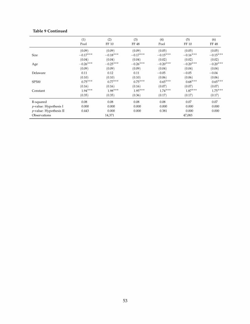
Table 9 Continued

(1) (2) (3) (4) (5) (6)Pool FF 10 FF 48 Pool FF 10 FF 48

(0.09) (0.09) (0.09) (0.05) (0.05) (0.05)Size −0.17∗∗∗ −0.18∗∗∗ −0.17∗∗∗ −0.15∗∗∗ −0.16∗∗∗ −0.15∗∗∗

(0.04) (0.04) (0.04) (0.02) (0.02) (0.02)Age −0.26∗∗∗ −0.25∗∗∗ −0.26∗∗∗ −0.20∗∗∗ −0.20∗∗∗ −0.20∗∗∗

(0.09) (0.09) (0.09) (0.04) (0.04) (0.04)Delaware 0.11 0.12 0.11 −0.05 −0.05 −0.04

(0.10) (0.10) (0.10) (0.06) (0.06) (0.06)SP500 0.75∗∗∗ 0.77∗∗∗ 0.75∗∗∗ 0.65∗∗∗ 0.68∗∗∗ 0.65∗∗∗

(0.16) (0.16) (0.16) (0.07) (0.07) (0.07)Constant 1.94∗∗∗ 1.98∗∗∗ 1.95∗∗∗ 1.74∗∗∗ 1.87∗∗∗ 1.75∗∗∗

(0.35) (0.35) (0.36) (0.17) (0.17) (0.17)

R-squared 0.08 0.08 0.08 0.08 0.07 0.07p-value: Hypothesis I 0.000 0.000 0.000 0.000 0.000 0.000p-value: Hypothesis II 0.443 0.000 0.000 0.381 0.000 0.000Observations 14,371 47,083

53

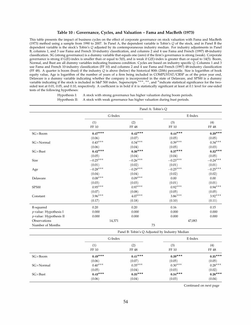
Table 10 : Governance, Cycles, and Valuation – Fama and MacBeth (1973)

This table presents the impact of business cycles on the effect of corporate governance on stock valuation with Fama and MacBeth(1973) method using a sample from 1990 to 2007. In Panel A, the dependent variable is Tobin’s Q of the stock, and in Panel B thedependent variable is the stock’s Tobin’s Q adjusted by its contemporaneous industry median. For industry adjustments in PanelB, columns 1, and 3 use Fama and French 10-industry classification, and columns 2 and 4 use Fama and French (1997) 48-industryclassification. SG (strong governance) is a dummy variable that equals one (zero) if the firm’s governance is strong (weak). Corporategovernance is strong if G(E)-index is smaller than or equal to 5(0), and is weak if G(E)-index is greater than or equal to 14(5). Boom,Normal, and Bust are all dummy variables indicating business condition. Cycles are based on industry specific Q. Columns 1 and 3use Fama and French 10-industry classification (FF 10) and columns 2 and 4 use Fama and French (1997) 48-industry classification(FF 48). A quarter is boom (bust) if the industry Q is above (below) the historical 80th (20th) percentile. Size is logarithm of bookequity value, Age is logarithm of the number of years of a firm being included in COMPUSTAT/CRSP as of the prior year end,Delaware is a dummy variable indicating whether the company is incorporated in the state of Delaware, and SP500 is a dummyvariable indicating if the stock is included in S&P 500 index. Superscripts ∗∗∗, ∗∗, and ∗indicate statistical significance for the two-sided test at 0.01, 0.05, and 0.10, respectively. A coefficient is in bold if it is statistically significant at least at 0.1 level for one-sidedtests of the following hypotheses:

Hypothesis I: A stock with strong governance has higher valuation during boom periods.Hypothesis II: A stock with weak governance has higher valuation during bust periods.

Panel A: Tobin’s Q

G-Index E-Index

(1) (2) (3) (4)FF 10 FF 48 FF 10 FF 48

SG×Boom 0.47∗∗∗ 0.42∗∗∗ 0.44∗∗∗ 0.39∗∗∗

(0.06) (0.07) (0.05) (0.05)SG×Normal 0.43∗∗∗ 0.34∗∗∗ 0.39∗∗∗ 0.34∗∗∗

(0.06) (0.04) (0.05) (0.03)SG×Bust 0.42∗∗∗ 0.36∗∗∗ 0.37∗∗∗ 0.32∗∗∗

(0.05) (0.04) (0.04) (0.05)Size −0.25∗∗∗ −0.26∗∗∗ −0.23∗∗∗ −0.24∗∗∗

(0.01) (0.02) (0.01) (0.01)Age −0.28∗∗∗ −0.29∗∗∗ −0.25∗∗∗ −0.25∗∗∗

(0.04) (0.04) (0.02) (0.02)Delaware 0.08∗∗∗ 0.09∗∗∗ 0.00 0.00

(0.03) (0.03) (0.01) (0.01)SP500 0.95∗∗∗ 0.97∗∗∗ 0.92∗∗∗ 0.94∗∗∗

(0.07) (0.08) (0.05) (0.05)Constant 3.96∗∗∗ 4.07∗∗∗ 3.86∗∗∗ 3.92∗∗∗

(0.17) (0.18) (0.10) (0.11)

R-squared 0.20 0.20 0.16 0.15p-value: Hypothesis I 0.000 0.000 0.000 0.000p-value: Hypothesis II 0.000 0.000 0.000 0.000Observations 14,371 47,083Number of Months 73

Panel B: Tobin’s Q Adjusted by Industry Median

G-Index E-Index

(1) (2) (3) (4)FF 10 FF 48 FF 10 FF 48

SG×Boom 0.49∗∗∗ 0.41∗∗∗ 0.39∗∗∗ 0.35∗∗∗

(0.06) (0.07) (0.05) (0.05)SG×Normal 0.40∗∗∗ 0.35∗∗∗ 0.30∗∗∗ 0.28∗∗∗

(0.05) (0.04) (0.03) (0.02)SG×Bust 0.43∗∗∗ 0.35∗∗∗ 0.34∗∗∗ 0.26∗∗∗

(0.06) (0.04) (0.03) (0.04)

Continued on next page

54

Table 10 Continued

(1) (2) (3) (4)FF 10 FF 48 FF 10 FF 48

Size −0.17∗∗∗ −0.17∗∗∗ −0.16∗∗∗ −0.15∗∗∗(0.01) (0.01) (0.01) (0.01)

Age −0.22∗∗∗ −0.23∗∗∗ −0.20∗∗∗ −0.19∗∗∗(0.03) (0.03) (0.02) (0.02)

Delaware 0.09∗∗∗ 0.09∗∗∗ −0.04∗∗∗ −0.04∗∗∗(0.02) (0.03) (0.01) (0.01)

SP500 0.74∗∗∗ 0.74∗∗∗ 0.70∗∗∗ 0.68∗∗∗(0.07) (0.07) (0.04) (0.05)

Constant 1.86∗∗∗ 1.90∗∗∗ 1.85∗∗∗ 1.76∗∗∗(0.15) (0.15) (0.07) (0.08)

R-squared 0.14 0.14 0.10 0.10p-value: Hypothesis I 0.000 0.000 0.000 0.000p-value: Hypothesis II 0.000 0.000 0.000 0.000Observations 14,371 47,083Number of Months 73

55