Corporate Governance and Capital Structure Dynamics:

Evidence from Structural Estimation ∗

Erwan Morellec† Boris Nikolov‡ Norman Schurhoff§

July 2010

∗We thank an anonymous referee, the associate editor, the editor (Campbell Harvey), and DarrellDuffie for many valuable comments and Julien Hugonnier for suggesting an elegant approach to thecalculation of conditional densities in our setting. We also thank Tony Berrada, Peter Bossaerts, BernardDumas, Michael Lemmon, Marco Pagano, Michael Roberts, Rene Stulz, Toni Whited, Marc Yor, JeffZwiebel, and seminar participants at Boston College, Carnegie Mellon University, HEC Paris, the LondonSchool of Economics, the University of Colorado at Boulder, the University of Lausanne, the Universityof Rochester, the 2008 American Finance Association meetings, 2008 North American Summer Meetingsof the Econometric Society, and the conference on “Understanding Corporate Governance” organized bythe Fundacion Ramon Aceres in Madrid for helpful comments. The three authors acknowledge financialsupport from the Swiss Finance Institute and from NCCR FINRISK of the Swiss National ScienceFoundation.

†Swiss Finance Institute, Ecole Polytechnique Federale de Lausanne (EPFL), and CEPR. E-mail:erwan.morellec@epfl.ch. Postal: Ecole Polytechnique Federale de Lausanne, Extranef 210, QuartierUNIL-Dorigny, CH-1015 Lausanne, Switzerland.

‡William E. Simon Graduate School of Business Administration, University of Rochester. E-mail:boris.nikolov@simon.rochester.edu. Postal: Simon School of Business, University of Rochester, NY 14627Rochester, USA.

§Swiss Finance Institute, University of Lausanne, and CEPR. E-mail: norman.schuerhoff@unil.ch.Postal: Ecole des HEC, University of Lausanne, Extranef 239, CH-1015 Lausanne, Switzerland.

Abstract

We estimate a dynamic capital structure model to ascertain whether agency conflicts canexplain corporate financing decisions. The model features corporate and personal taxes, refi-nancing and liquidation costs, costly debt renegotiation, and allows managers to capture partof the firm’s cash flows as private benefits within the limits imposed by shareholder protec-tion. The analysis demonstrates that private benefits of control lead managers to issue lessdebt and rebalance capital structure less often than optimal for shareholders. Using data onfinancing choices and the model’s predictions for different moments of leverage, we find thatprivate benefits or agency costs of 1.02% of equity value on average (0.23% at median) are suf-ficient to resolve the conservative debt policy puzzle and to explain the time series of observedleverage ratios. We also find that the variation in agency costs across firms is sizeable and thatgovernance mechanisms significantly affect the value of control and firms’ financing decisions.

JEL Classification Numbers: G12; G31; G32; G34.

A central theme in financial economics is that incentive conflicts within the firm lead to dis-

tortions in corporate policy choices and, as a result, to lower corporate valuations. Because

debt limits managerial flexibility (Jensen, 1986), a particular focus of the theoretical research

has been on the importance of managerial objectives in the workings of financing decisions. A

prevalent view in the literature is that managers do not always make capital structure decisions

that maximize shareholder wealth. The capital structure of a firm should then be determined

not only by real market frictions, such as taxes, bankruptcy costs, or refinancing costs, as in

the seminal work of Fisher, Heinkel, and Zechner (1989), but also by the severity of incentive

conflicts between managers and shareholders. A variety of empirical evidence lends support to

this view.1 However, after more than two decades of research, how much do we really know

about the magnitude of manager-shareholder conflicts? In addition, how much do we know

about their effects on the dynamics and cross section of corporate capital structure?

The goal of this paper is to address these and related questions by exploiting the structural

restrictions from a dynamic capital structure model. To do this, we begin by formulating a

dynamic tradeoff model that emphasizes the role of agency conflicts in shaping firms’ financing

decisions. The model features corporate and personal taxes, refinancing costs, liquidation costs,

and costly renegotiation of debt in distress. In the model, each firm is run by a manager who

sets the firm’s financing, restructuring, and default policies. Managers act in their own interests

and can capture part of the firm’s cash flows as private benefits within the limits imposed by

shareholder protection. In this environment, we determine the optimal leveraging decision of

managers and characterize the effects of incentive conflicts between managers and shareholders

on financing decisions. We then use panel data on observed leverage choices and the model’s

predictions for different statistical moments of financial leverage to obtain firm-specific estimates

of unobserved private benefits of control.

Several important results follow from this analysis. First, we show how various capital

market imperfections interact with firms’ incentives structures to determine financing deci-

sions. This allows us to derive testable implications relating manager-shareholder conflicts to

a firm’s target leverage as well as the pace and size of capital structure changes. Second, we

infer the magnitude of agency conflicts from data on leverage choices. Specifically, we provide

1For example, Jung, Kim, and Stulz (1996) identify security issue decisions that seem inconsistent withshareholder value maximization. Friend and Lang (1988), Mehran (1992), Berger, Ofek, and Yermak (1997), andKayhan (2008) find that leverage levels are lower when CEOs do not face pressure from the market for corporatecontrol. Berger, Ofek, and Yermak also find that leverage increases in the aftermath of shocks reducing managerialentrenchment. Garvey and Hanka (1999) find that firms protected by “second generation” state antitakeoverlaws substantially reduce their use of debt, and that unprotected firms do the reverse.

1

firm-specific estimates of agency costs and relate these estimates to the firms’ governance struc-

ture. The agency conflicts identified from the data have an economically significant order of

magnitude, exhibit sizeable variation across firms, and vary with various proxies for corporate

governance. Third, we show that by accounting for agency conflicts in dynamic tradeoff mod-

els, and giving the manager control of the leverage decision, one can obtain capital structure

dynamics consistent with the data. Specifically, manager-shareholder conflicts can explain why

some firms issue little debt despite the known tax benefits of debt—the conservative debt policy

puzzle (see Graham, 2000), and why leverage ratios exhibit inertia and other robust time-series

patterns (see Fama and French, 2002, Welch, 2004, or Flannery and Rangan, 2006).

As in prior dynamic tradeoff models, our analysis emphasizes the role of external financing

costs in affecting the time series of leverage ratios. Due to capital market frictions, firms are not

able to keep their leverage at the target at all times. As a result, leverage is best described not

just by a number, the target, but by its entire distribution—including target and refinancing

boundaries. The model also reflects the interaction between real market frictions and manager-

shareholder conflicts, allowing us to generate a number of novel predictions relating agency

conflicts to the firm’s target leverage, the frequency and size of capital structure changes, and

the likelihood of default. Notably, our model predicts that incentive conflicts between managers

and shareholders lower the firm’s target leverage and raise the refinancing cash-flow trigger. As a

consequence, the range of leverage ratios widens and financial inertia becomes more pronounced

as agency conflicts increase. The intuition behind these results is that managers choose capital

structure to maximize the sum of their equity stake and the present value of private benefits.

Since debt constrains managers by limiting the cash flows available as private benefits (as in

Jensen, 1986, Zwiebel, 1996, or Morellec, 2004), managers issue less debt (lower target and

default cash-flow trigger) and restructure less frequently (higher refinancing cash-flow trigger)

than optimal for shareholders.

The paper also provides new evidence on the relation between governance mechanisms and

capital structure dynamics. Specifically, we use observed financing choices to provide firm-

specific estimates of manager-shareholder conflicts. We exploit not only the conditional mean

of leverage (as in a regression) but also the variation, persistence and distributional tails—in

short, the conditional moments of the time-series distribution of leverage. Using structural

econometrics, we find that agency costs of 1.02% of equity value for the average firm are

sufficient to resolve the conservative debt policy puzzle and explain the time series of observed

leverage ratios. We also find that the variation in agency costs across firms is substantial. Thus,

2

while leverage ratios tend to revert to the (manager’s) target leverage over time, the variation

in agency conflicts leads to persistent cross-sectional differences in leverage ratios, in line with

Lemmon, Roberts, and Zender (2008).

To make the analysis of capital structure determinants complete, we also introduce shareholder-

debtholder conflicts in our setting. In the model, shareholders can renegotiate outstanding

claims in default as in Fan and Sundaresan (2000). Our structural estimates reveal that the

bargaining power of shareholders in default is close to the Nash solution for the average firm.

Hence, shareholders can extract substantial concessions from debtholders in default. However,

while shareholder-debtholder conflicts reduce leverage, we find that they have little effect on

the cross-sectional variation and on the dynamics of leverage ratios.

The analysis in the present paper relates to the literature that analyzes the relation between

manager-shareholder conflicts and firms’ financing decisions.2 The paper that is closest to ours

is Zwiebel (1996) in that it also builds a dynamic capital structure model in which financing

policy is selected by a partially-entrenched manager. However, while firms are always at their

target leverage in Zwiebel’s model, refinancing costs create inertia and persistence in capital

structure in our model. Second, this paper relates to the dynamic contingent claims models of

Fisher, Heinkel, and Zechner (1989), Goldstein, Ju, and Leland (2001), or Strebulaev (2007).

In this literature, conflicts of interest between managers and shareholders have been largely

ignored (see however the static models of Morellec, 2004, or Lambrecht and Myers, 2008).

Our model also relates to the tradeoff models of Hennessy and Whited (HW 2005, 2007).

Their models consider the role of internally generated funds. However they do not allow for

default (HW, 2005) and ignore manager-shareholder conflicts. Another important difference is

that our closed-form expression for the time-series distribution of leverage ratios allows us to

look at all statistical moments of the leverage distribution (including target leverage, refinanc-

ing frequency, and default probability) instead of focusing on a limited number of moments.

Finally, our paper is related to the analysis in Lemmon et al. (2008), who find that traditional

determinants of leverage account for relatively little of the variation in capital structure. In-

stead they show that the majority of the cross-sectional variation in capital structures is driven

by an unexplained firm-specific determinant. Our analysis reveals that the heterogeneity in

capital structure can be structurally related to a number of corporate governance mechanisms,

providing an economic interpretation for their results.

2See Stulz (1990), Chang (1993), Hart and Moore (1994, 1995), Zwiebel (1996), Morellec (2004), or Barclay,Morellec, and Smith (2006). This literature has provided a rich intuition on the effects of managerial discretionon financing decisions, it has been so far mostly qualitative, focusing on directional effects.

3

This paper advances the literature on financing decisions in two important dimensions.

First, we develop the first dynamic model of capital structure decisions that includes taxes,

bankruptcy costs, refinancing costs, and agency conflicts. This allows us to derive clear testable

predictions regarding the effects of these various determinants of financing policies on target

leverage and the pace and size of capital structure changes. Second, and more importantly, our

analysis adds to the literature by providing firm-specific estimates of agency conflicts, and by

showing that the separation between ownership and control can explain the conservative debt

policy puzzle as well as the dynamics of leverage ratios.

The remainder of the paper is organized as follows. Section I describes the model. Section II

discusses the data and our empirical methodology. Section III provides firm-specific estimates of

manager-shareholder conflicts and shareholder bargaining power in default. Section IV explores

how well the model fits the time series and cross section of financial leverage. Section V

relates the estimates of agency conflict to various corporate governance mechanisms. Section VI

concludes. Technical developments are gathered in an Appendix.

I. The Model

Most capital structure models make the simplifying assumption that managers choose capital

structure in the interests of shareholders. Recently, however, research into capital structure

has explicitly recognized that managers’ self interest can lead to financial policies that do not

maximize shareholder wealth. This section presents a model of firms’ financing decisions that

extends the contingent claims framework to incorporate manager-shareholder conflicts. In the

following sections, we use this model to obtain firm-specific estimates of agency conflicts.

A. Assumptions

The model closely follows Leland (1998) and Strebulaev (2007). Throughout the paper, assets

are continuously traded in complete and arbitrage-free markets. The default-free term structure

is flat with an after-tax risk-free rate r, at which investors may lend and borrow freely.

We consider an economy with a large number of heterogeneous firms, indexed by i =

1, . . . , N . Firms are infinitely lived and have monopoly access to a set of assets, that are

operated in continuous time. The firm-specific state variable is the cash flow generated by the

4

operation of the firm’s assets, denoted by Xi. This operating cash flow is independent of capital

structure choices and governed, under the risk neutral probability measure Q, by the process:3

dXit = µiXit dt + σiXit dBit , Xi0 = xi0 > 0, (1)

where µi < r and σi > 0 are constants and (Bit)t≥0 is a standard Brownian motion. Equation

(1) implies that the growth rate of cash flows is Normally distributed with mean µi∆t and

variance σ2i ∆t over the time interval ∆t under the risk-neutral probability measure. It also

implies that the mean growth rate of cash flows is mi∆t = (µi + βiψ)∆t under the physical

probability measure, where βi is the unlevered cash-flow beta and ψ is the market risk premium.

Cash flows from operations are taxed at a constant rate τ c. As a result, firms may have an

incentive to issue debt to shield profits from taxation. To stay in a simple time-homogeneous

setting, we consider debt contracts that are characterized by a perpetual flow of coupon pay-

ments c and a principal P . Debt is callable and issued at par. The proceeds from the debt issue

are distributed on a pro rata basis to shareholders at the time of flotation. We consider that

firms can adjust their capital structure upwards at any point in time by incurring a proportional

cost λ, but that they can reduce their indebtedness only in default.4 Under this assumption,

the firm’s initial debt structure remains fixed until either the firm goes into default or the firm

calls its debt and restructures with newly issued debt. The personal tax rate on dividends

τd and on coupon payments τ i are identical for all investors. These features are shared with

numerous other capital structure models, including Leland (1998), Goldstein, Ju, and Leland

(2001), Hackbarth, Miao, and Morellec (2006), or Strebulaev (2007).

We are interested in building a model in which financing choices reflect not only the tradeoff

between the tax benefits of debt and contracting costs, but also agency conflicts. Agency

3This corresponds to a reduced-form specification of a model in which the firm is allowed to invest in newassets at any time t ∈ (0,∞) and investment is perfectly reversible. To see this, assume that the firm’s assetsproduce output with the production function F : R+ → R+, F (kt) = kγ

t , where γ ∈ (0, 1) and that capitaldepreciates at a constant rate δ > 0. Define the firm’s after tax profit function fit by

fit = maxk≥0

[(1 − τ ci )(Xitk

γt − δkt) − rkt].

Solving this maximization problem for kt and replacing kt by its expression in the firm’s after-tax profit functiongives fit = (1 − τ c

i )Yit where (Yit)t≥0is a (capacity-adjusted cash flow) shock governed by

dYit = µY Yitdt + σY YitdWt, Yi0 = AXi0 > 0.

where µY = ϑµi + ϑ(ϑ − 1)σ2i /2, σY = ϑσi, and (A,ϑ) ∈ R

2++ are constant parameters.

4While in principle management can both increase and decrease future debt levels, Gilson (1997) finds thattransaction costs discourage debt reductions outside of renegotiation.

5

conflicts between the manager and shareholders are introduced by considering that each firm

is run by a manager who can capture a fraction φ ∈ [0, 1) of free cash flow to equity as private

benefits (as in La Porta, Lopez-de Silanes, Shleifer, and Vishny (2002), Lambrecht and Myers

(2008), or Albuquerque and Wang (2008)). That is, the unadjusted cash flows to equity are

(1− τ c)(Xt − c), of which shareholders receive a fraction (1−φ) and management appropriates

a fraction φ. This cash diversion or tunneling of funds toward socially inefficient usage may

take a variety of forms such as excessive salary, transfer pricing, employing relatives and friends

who are not qualified for the jobs in the firm, and perquisites, just to name a few. In the model,

we take φ as a fixed, exogenous parameter that reflects the severity of manager-shareholder

conflicts. When φ = 0 there is no agency conflict and managers and shareholders agree about

corporate policies. Our objective in the empirical section is to estimate the magnitude of φi,

i = 1, . . . , N , and to relate our estimates to corporate governance mechanisms.

Firms whose conditions deteriorate sufficiently may default on their debt obligations. In

the model, default can lead either to liquidation or to renegotiation. At the time of default,

a fraction of assets are lost as a frictional cost, leading to a reduction in operating cash flows.

Specifically, we consider that if the instant of default is T , then XT = (1 − α)XT− in case of

liquidation and XT = (1−κ)XT− in case of reorganization, with 0 ≤ κ < α. We assume that in

case of reorganization, manager-shareholder conflicts are unaffected by default. Because liqui-

dation is more costly than reorganization, there exists a surplus associated with renegotiation.

This surplus represents a fraction (α − κ) of cash flows after default. Following Fan and Sun-

daresan (2000), we consider a Nash bargaining game in default that leads to a debt-equity swap.

We denote the bargaining power of shareholders by η ∈ [0, 1]. Assuming that the renegotiation

surplus is shared according to a sharing rule , the generalized Nash bargaining solution is

simply given by = η, so that the shareholders get a fraction η (α− κ) of cash flows after

default. In addition to the estimates of φi, the paper provides estimates of ηi, i = 1, . . . , N .

Agency costs of managerial discretion typically depend on the allocation of control rights

within the firm. In this paper, we follow Zwiebel (1996), Morellec (2004), and Lambrecht and

Myers (2008) by considering that the manager owns a fraction ϕ of the firm’s equity and has

decision rights over the firm’s initial debt structure and the firm’s restructuring and default

policies. When making policy choices, managers act in their own interests to maximize the

present value of the total expected cash flows (managerial rents and equity stake) that they will

take from the firm’s operations. As in Leland (1998) and Strebulaev (2007), the firm’s initial

debt structure remains fixed until either the firm’s cash flows reach a low level that the firm

6

goes into default or the cash flows rise to a sufficiently high level that the manager calls the debt

and restructures with newly issued debt. In the analysis below, we will denote by xD (< x0)

the default threshold and by xU (> x0) the restructuring threshold selected by the manager.

We can thus view the manager’s policy choices as determining the initial coupon payment c,

the restructuring threshold xU , and the default boundary xD.

B. Model Solution

Before solving the manager’s optimization problem, it will be useful to derive explicit expressions

for the value of corporate securities. In the model, the cash flow accruing to the manager at each

time t is given by [φ+ ϕ(1 − φ)] (1−τ)(Xt−c), where the tax rate τ = 1−(1−τ c)(1−τd) reflects

corporate and personal taxes. Shareholders’ cash flows are in turn given by (1−φ)(1−τ)(Xt−c).That is, shareholders receive the cash flows from operations minus the coupon payment c, the

cash flows captured by the manager, and the taxes paid on corporate and personal income.

Since managers and shareholders are entitled to a cash flow stream that is proportional to the

firm’s net income (1 − τ)(Xt − c), we start by deriving the value of a claim on net income at

time t, denoted by N(x, c) for Xt = x.

Let n (x, c) denote the present value of the firm’s net income over one financing cycle, i.e.,

for the period over which neither the default threshold xD nor the restructuring threshold xU

are hit and the firm does not change its debt policy. This value is given by

n(x, c) = EQ[ ∫ T

te−r(s−t) (1 − τ) (Xs − c) ds|Xt = x

], (2)

where T is the first time that the firm changes its debt policy, defined by T = inf {TU , TD} with

Ts = inf {t ≥ 0 : Xt = xs}, s = U,D. This expression gives the value of a claim to the firm’s

net income until either the firm increases its debt level to shield more profits from taxation or

the firm defaults on its debt obligations. This value does not incorporate any of the cash flows

that accrue to claimholders after a restructuring. These cash flows belong to the next financing

cycle and will be incorporated in the total value of the claim to net income, N(x, c).

Denote by pU (x) the present value of $1 to be received at the time of refinancing, contingent

on refinancing occurring before default, and by pD (x) the present value of $1 to be received at

7

the time of default, contingent on default occurring before refinancing. Using this notation, we

can write the solution to equation (2) as:

n(x, c) = (1 − τ)

[x

r − µ− c

r− pU (x)

(xU

r − µ− c

r

)− pD (x)

(xD

r − µ− c

r

)], (3)

where [see Revuz and Yor (1999, pp. 72)]

pD (x) =xξ − xνxξ−ν

U

xξD − xν

Dxξ−νU

and pU (x) =xξ − xνxξ−ν

D

xξU − xν

Uxξ−νD

and ξ and ν are the positive and negative roots of the equation 12σ

2β (β − 1) + µβ − r = 0.

The first two terms in the square bracket of equation (3) represent the value of a perpetual

entitlement to net income. The other terms reflect the fact that payments are stopped after

either a restructuring (third term) or a default (fourth term).

Consider next the total value N (x, c) of a claim to the firm’s net income. We show in the

Internet Appendix that in the static model in which the firm cannot restructure, the default

threshold xD is linear in the coupon payment c. In addition, the selected coupon rate c is linear

in x. This implies that if two firms i and j are identical except that xi0 = Λxj

0, then the selected

coupon rate and default threshold satisfy ci = Λcj and xiD = Λxj

D, respectively, and every claim

will be scaled by the same factor Λ.

For the dynamic model, this scaling feature implies that at the first restructuring point, all

claims are scaled up by the same proportion ρ ≡ xU/x0 as asset value has increased (i.e., it is

optimal to choose c1 = ρc0, x1D = ρx0

D, x1U = ρx0

U ). Subsequent restructurings scale up these

variables again by the same ratio. If default occurs prior to restructuring, firm value is reduced

by a constant factor η (α− κ) γ with γ ≡ xD/x0, new debt is issued, and all claims are scaled

down by the same proportion η(α− κ)γ. As a result, we have for xD ≤ x ≤ xU :

N (x, c) = n (x, c)︸ ︷︷ ︸ + pU (x) ρN (x0, c)︸ ︷︷ ︸ + pD (x) η (α− κ) γN (x0, c)︸ ︷︷ ︸ .

Total value Value over PV of claim on net PV of claim on net

of the claim one cycle income at a restructuring income in default

(4)

This equation shows that the value of a claim to the firm’s net income over all financing cycles

is equal to the cash flows claimholders receive over one financing cycle plus the value of the

cash flows they get after the restructuring or in default. Using this expression, we can express

8

the total value of a claim to the firm’s net income at the initial date as:

N (x0, c) =n (x0, c)

1 − pU (x0) ρ− pD (x0) η (α− κ) γ≡ n (x0, c) S(x0, ρ, γ), (5)

where S(x0, ρ, γ) is a scaling factor that transforms the value of a claim to cash flows over one

financing cycle at a restructuring point into the value of this claim over all financing cycles.

The same arguments apply to the valuation of corporate debt. Consider first the value

d (x, c) of the debt issued at time t = 0. Since the issue is called at par if the firm’s cash flows

reach xU before xD, the current value of corporate debt satisfies at any time t ≥ 0:

d (x, c) = b (x, c)︸ ︷︷ ︸ + pU (x) d (x0, c)︸ ︷︷ ︸ .

Value of debt over one cycle PV of cash flow at a restructuring(6)

where b(x, c) represents the value of corporate debt over one refinancing cycle, i.e., ignoring the

value of the debt issued after a restructuring or after default, and is given by

b (x, c) =

(1 − τ i

)c

r[1 − pU (x) − pD (x)] + pD (x) [1 − (κ+ η (α− κ))]

(1 − τ

r − µ

)xD . (7)

The first term on the right-hand side of this equation represents the present value of the coupon

payments until the firm defaults or restructures (i.e., until time T ). The second term represents

the present value of the cash flow to initial debtholders in default.

As in the case of the claim to net income, the total value of corporate debt includes not

only the cash flows accruing to debtholders over one refinancing cycle, b(x, c), but also the

new debt that will be issued in default or at the time of a restructuring. As a result, the

value of the total debt claim over all the financing cycles is given by b(x0, c)S(x0, ρ, γ), where

S(x0, ρ, γ) is defined in equation (5). Because flotation costs are incurred each time the firm

adjusts its capital structure, the total value of adjustment costs at time t = 0 is in turn given

by λd (x0, c) S(x0, ρ, γ). We can then write the value of the firm at the restructuring date as

the sum of the present value of a claim on net income plus the value of all debt issues minus

the present value of issuance costs and the present value of managerial rents, or

V (x0, c) = S(x0, ρ, γ) {n (x0, c) + b (x0, c) − λd (x0, c) − φn (x0, c) } . (8)

We are now in a position to determine the manager’s policy choices. Denote the present

value of the manager’s cash flows for a current value of the cash-flow shock x by M(x, c). This

9

value is the sum of the manager’s equity stake and the value of private benefits. The value of

equity at the time of debt issuance is equal to total firm value, V(x, c), because debt is fairly

priced. Assuming that managers stay in control after default,5 we can then express the total

value of the manager’s claims as:

M(x, c) = ϕV(x, c)︸ ︷︷ ︸ + φN(x, c)︸ ︷︷ ︸ ,

Equity stake PV of managerial rents(9)

where ϕ represents the fraction of the firm’s equity owned by the manager and φ represents the

fraction of the firm’s net income that can be captured by the manager.

When choosing financing policy, the objective of the manager is to maximize the ex-ante

value of his claims by selecting the coupon payment c and the scaling factor ρ = xU/x0. Thus,

the manager solves

supc,ρ

M(x, c) = supc,ρ

{ϕV(x, c) + φN(x, c)} . (10)

Since N(x, c) decreases with c, equation (9) implies that the efficient choice of debt (optimal

for shareholders) differs from the manager’s choice of debt whenever φ > 0. In particular, the

model predicts that the coupon payment decreases with φ and that the debt level selected by

the manager is lower than the debt level that maximizes firm value.

In a rational expectations model, the solution to the problem (10) reflects the fact that

following the flotation of corporate debt, the manager chooses a default policy that maximizes

the value of his claim after debt has been issued. As in Leland (1998) or Strebulaev (2007), the

selected default threshold results from a tradeoff between continuation value outside of default

and the value of claims in default. Since all claims are scaled down by the same factor in default,

the manager and shareholders agree on the firm’s default policy. The value of equity at the

time of default satisfies V(x, c) − d (x, c) = η (α− κ) γV(x, c) (value-matching). The default

threshold can then be determined by solving the smooth-pasting condition:

∂ [V(x, c) − d (x, c)]

∂x

∣∣∣∣x=xD

=∂η (α− κ) γV(x, c)

∂x

∣∣∣∣x=xD

. (11)

The full problem of managers thus consists of solving (10) subject to (11). A closed-form

solution to this problem does not exist and thus standard numerical procedures are used.

5This assumption reflects the fact that managers usually stay in control after debt is renegotiated privatelyor after court supervised debt renegotiation (see e.g. Gilson, 1989, for empirical evidence).

10

II. Empirical Analysis

In this section, we estimate the model derived in Section I using data on financial leverage. Our

objective is to ascertain whether agency conflicts can explain the debt conservatism puzzle as

well as the time-series patterns in observed leverage ratios. To do so, we exploit the structural

restrictions of the model and estimate from panel data on financing decisions the level of agency

conflicts that best explain observed financing behavior (a similar approach is used in Hennessy

and Whited, 2007). In a second stage, we examine whether these estimates are related to

variables reflecting the quality of a firm’s governance structure.

A. Data

Estimating the model derived in Section I requires merging data from various standard sources.

We collect financial statements from Compustat, managerial compensation data from Execu-

Comp, stock price data from CRSP, analyst forecasts from I/B/E/S, governance data from

IRRC, and institutional ownership data from Thomson Reuters. Following the literature, we

remove all regulated (SIC 4900−4999) and financial firms (SIC 6000−6999). Observations with

missing SIC code, total assets, market value, sales, long-term debt, debt in current liabilities are

also excluded. In addition, we restrict our sample to firms that have total assets over $10 mil-

lion. As a result of these selection criteria, we obtain a panel dataset with 13, 159 observations

for N = 809 firms, for the time period from 1992 to 2004 at the quarterly frequency. Tables I

and II provide detailed definitions and descriptive statistics for the variables of interest.

Insert Tables I and II Here

In the analysis, each firm i = 1, . . . , N is characterized by a set of parameters θi =

(mi, µi, σi, βi, αi, κi, ϕi, λi, τc, τ i, τd, ψ, r, φi, ηi) ∈ Θ. The subscript i indicates that the pa-

rameter values are firm-specific. Otherwise the parameter takes a single, economy-wide value.

The different parameters determine the growth rate mi (µi under the risk-neutral measure)

and volatility σi of the firm’s cash flows, the liquidation and reorganization costs (αi, κi), the

manager’s equity stake ϕi, the refinancing cost λi, and the tax environment (τ c, τ i, τd). The

parameters of interest—capturing different sources of agency conflicts—are the fraction of cash

flows captured by the manager φi and the bargaining power of shareholders in default ηi.

11

Estimating the entire parameter vector θi for each firm i = 1, . . . , N using solely data on

financial leverage is unnecessary and practically infeasible. We therefore split the parameter

vector into two parts: nuisance parameters and deep (agency) parameters that we estimate

structurally. Given the dimensionality of the empirical estimation problem, we first determine

the nuisance parameters θ⋆i = (mi, µi, σi, βi, αi, κi, ϕi, λi, τ

c, τ i, τd, ψ, r) using the above data

sources. We then keep the nuisance parameters θ⋆i fixed when estimating the deep parameters

(φi, ηi) from data on financial leverage. Since the estimators of θ⋆i are

√n-consistent for a

sample of size n, consistency of our estimates of the structural parameters is unaffected by

assuming we can estimate or construct proxies for the true values of θ⋆i . We investigate the

effect of sampling error in θ⋆i on our estimates of agency cost parameters in Section III.B below.

We construct the estimates of the nuisance parameters as follows. In our base case esti-

mation, we first compute period-by-period estimates for each firm. Since the model is writ-

ten in terms of constant firm level parameters, we then average the time-specific estimates

(mit, µit, σit, αit, βit, ϕit) over the sample period for each firm to obtain the set the parameters

(mi, µi, σi, αi, βi, ϕi) (i.e., θ⋆i = 1

ni

∑ni

t=1 θ⋆it for i = 1, . . . , N , where ni is the number of observa-

tions). In Section III.C, we check whether our estimation results depend on this assumption.

We proxy the growth rate of cash flows, m, by an affine function of the mean long-term

growth rate per industry, m, where we use SIC level 2 to define industries. The Institutional

Brokers’ Estimate System (IBES) provides analysts’ forecasts for the long-term growth rate.

It is generally agreed, however, that IBES consensus long-term growth rates are too optimistic

compared to realized growth. In addition, Chan, Karceski, and Lakonishok (CKL, 2003) show

that IBES predicts too much cross-sectional variation in growth rates. Following CKL (2003),

we adjust for these two biases by using the following least-squares predictor for the cash-flow

growth rate: mit = 0.007264043+0.408605737× mit . We then estimate the growth rate of firm

i by the time-series average mi = 1ni

∑ni

t=1mit. Using data on IBES consensus forecasts in our

sample, we can predict the actual growth rates reasonably well with this linear specification;

our estimates are in line with the values reported in CKL (2003).

Next, we use the Capital Asset Pricing Model (CAPM) to estimate the risk-neutral growth

rate of cash flows: µit = mit − βitψt, where ψt is the market risk premium and βit is the

leverage-adjusted cash-flow beta. We estimate market betas from monthly equity returns and

unlever them using the model-implied relations. Similarly, we estimate cash-flow volatility σit

using the standard deviation of monthly equity returns and the following relation (implied by

12

It’s lemma): σit = σEit/(

∂E(x,c)∂x

xE(x,c)), where σE

it is the volatility of stock returns and E(x, c) ≡V(x, c) − d (x, c) is the stock price derived from the model. In these estimations, we use stock

returns from the Center for Research in Security Prices (CRSP) database.

ExecuComp provides data on managerial compensation schemes, allowing us to measure the

extent to which managerial incentives are aligned with shareholders’ interests (as reflected by ϕi

in our model). We construct several firm-specific measures of managerial ownership. Following

Core and Guay (1999), we construct the managerial delta, defined as the sensitivity of option

value to a one percent change in the stock price, for each manager and then aggregate over the

five highest-paid executives. In addition, following Jensen and Murphy (1990), we construct

a managerial incentives measure as the change in managerial wealth per dollar change in the

wealth of shareholders (see Appendix B for details):

ϕit = ϕEit + deltait

Shares represented by options awardsit

Shares outstandingit

. (12)

This incentives measure accounts for both a direct component, managerial share ownership ϕE ,

and an indirect component, the pay-performance sensitivity due to options awards.

The remaining parameters are standard. The risk-free rate r is based on the yield curve

of Treasury bonds during the sample period (r = 4.21%). The risk premium is set to the

consensus value of 6%. The relevant tax rates are based on estimates in Graham (1996). We

use the mean over the sample period for the tax rate on dividends and interest income, τd and

τ i, respectively. The tax rate on corporate income, τ c, is set to 35%. Gilson and Lang (1990)

find that renegotiation costs represent a small fraction of firm value. We thus fix renegotiation

costs κ to zero in our base case estimation (and to 15% in a robustness check). Following

Berger, Ofek, and Swary (1996), we estimate firm-specific liquidation costs, αit, as:

αit = 1 − (Tangibilityit + Cashit)/Total Assetsit. (13)

In equation (13), Berger, Ofek, and Swary (1996) estimate tangibility as Tangibilityit = 0.715

∗Receivablesit + 0.547∗Inventoryit + 0.535∗Capitalit.

Last, several studies provide estimates for issuance costs as a function of the amount of debt

being issued. The model, however, is written in terms of debt issuance cost λ as a fraction of

the total debt outstanding. The cost of debt issuance as a fraction of the issue size is given in

the model by ρρ−1λ, where ρ is the restructuring threshold multiplier. Since our estimates yield

13

a mean value of 2 for ρ, we set λ = 1%. This produces a cost of debt issuance representing

2% of the issue size on average, corresponding to the upper range of the values found in the

empirical literature (see e.g. Altinkilic and Hansen, 2000, and Kim, Palia, and Saunders, 2007).

B. Estimation Strategy and Empirical Specification

Our structural estimation of the deep parameters of the model uses simulated maximum likeli-

hood (SML) and exploits the panel nature of the data and the model’s predictions for different

moments of leverage. For an individual firm, the model implies a specific time-series behavior

of the firm’s leverage ratio. The policy predictions include the target leverage, the refinancing

frequency, and the default probability. In addition to the time-series predictions, the model

yields comparative statics that describe how financial policies and financial leverage vary in the

cross-section of firms. We exploit both types of predictions to identify the structural parame-

ters in the data and to disentangle cross-sectional heterogeneity from the impact of transaction

cost-driven inertia on financial leverage.

The main focus of inference is on the firm-specific private benefits of control φi and share-

holders’ bargaining power in default ηi. In the structural estimation, we treat these agency

parameters as random coefficients to reduce the dimensionality of the problem. Specifically, the

structural parameters characterizing agency conflicts are defined as:

φi = h(αφ + ǫφi ) and ηi = h(αη + ǫηi ), (14)

where h : R → [0, 1] is a transformation that guarantees that the parameters stay in their

natural domain6 and the ǫi = (ǫφi , ǫηi ) are bivariate random variables capturing the firm-specific

unobserved heterogeneity. As in linear dynamic random-effects models, the firm-specific random

effects ǫi are assumed independent across firms and, for all firms i = 1, . . . , N , are normally

distributed: ǫφi

ǫηi

∼ N

0,

σ2

φ σφη

σφη σ2η

. (15)

This setup is sufficiently flexible to capture cross-sectional variation in the parameter values

while imposing the model-implied structural restrictions on the domains of the parameters. In

summary, the set of structural parameters we need to estimate is θ = (αφ, αη , σφ, ση , σφη).

6In the base case, we use the standard normal cumulative distribution function Φ for h. Alternatively, we usethe inverse logit transformation. The results are similar and summarized in the section on robustness tests.

14

The likelihood function L of the parameters θ given the data and nuisance parameters θ⋆ is

based on the probability of observing the leverage ratio yit for firm i at date t. Assume that there

are N firms in the sample and let ni be the number of observations for firm i. The observations

for the same firm are correlated due to autocorrelation in the cash-flow process. Given these

assumptions, the joint probability of observing the leverage ratios yi = (yi1, . . . , yini)′ for firm

i and the firm-specific unobserved effects ǫi = (ǫφi , ǫηi ) is given by

f (yi, ǫi|θ) = f (yi|ǫi; θ) f (ǫi|θ)

=

(f(yi1|ǫi; θ)

ni∏

t=2

f(yit|yit−1, ǫi; θ)

)f (ǫi|θ) , (16)

where f(ǫi|θ) is the bivariate normal density corresponding to (15). Integrating out the ran-

dom effects from the joint likelihood f (y, ǫ|θ) =∏N

i=1 f (yi, ǫi|θ), we obtain the marginal log-

likelihood function (since the ǫi are drawn independently across firms from f(ǫi|θ)) as

lnL (θ; y) =

N∑

i=1

ln

∫

ǫi

(f(yi1|ǫi; θ)

ni∏

t=2

f(yit|yit−1, ǫi; θ)

)f (ǫi|θ) dǫi. (17)

For the model described in Section I, explicit expressions for the stationary density of

leverage f(yit|ǫi; θ) and conditional density f(yit|yit−1, ǫi; θ) can be derived (see Appendix A.1).

We evaluate the integral in equation (17) using Monte-Carlo simulations. When implementing

this procedure, we use the empirical analog to the log-likelihood function, which is given by

lnL (θ; y) =

N∑

i=1

ln1

K

K∑

ki=1

(f(yi1|ǫki

i ; θ)

ni∏

t=2

f(yit|yit−1, ǫki

i ; θ)

). (18)

In this equation, K is the number of random draws per firm, and ǫki

i is the realization in draw

ki for firm i. In Appendix C, we investigate how the precision and accuracy of the Monte-Carlo

simulations performed as part of the estimation depends on the number of random draws K

and how this affects the finite simulation sample bias in estimated coefficients. Figure 1 plots

the magnitude of the Monte-Carlo simulation error (Panel A) and its impact on the precision

and accuracy of the simulated log-likelihood (Panel B) as functions of K. We find that 1,000

random draws are sufficient to make the simulation error negligible. We thus set K = 1, 000 in

the estimations.

Insert Figure 1 Here

15

The SML estimator is now defined as: θ = arg maxθ lnL(θ; y). This estimator answers the

question: What magnitude of agency costs best explain observed financing patterns?

C. Model Predictions and Identification

Before proceeding to the empirical analysis, it will be useful to better understand how we iden-

tify in the data the parameters describing the (unobserved) agency conflicts. Our identification

strategy uses data on observable variables—corporate financing decisions—to infer properties

of unobserved variables—private benefits of control and shareholders’ bargaining power in de-

fault. In the following, we first illustrate the predictions of the model linking unobservables to

observables for a specific set of input parameter values. We then discuss more formally how

identification is obtained in our setting.

C.1. Model Predictions

In order to build intuition for the identification strategy, we start by reviewing the predictions of

the model with respect to firms’ financing decisions. Table III reports the firm’s target leverage,

the refinancing and default thresholds, the recovery rate in default, the corporate bond yield

spread at the leverage target, and the percentage increase in firm value due to tax savings

(the tax benefit of debt). Input parameter values for our base case are set as follows: the

risk-free interest rate r = 4.21%, the initial value of the cash flow shock x0 = 1 (normalized),

the growth rate and volatility of the cash flow shock µ = 1% and σ = 25%, the corporate

tax rate τ c = 35%, the tax rate on dividends τd = 11.6%, the tax rate on interest income

τ i = 29.3%, liquidation costs α = 50%, renegotiation costs κ = 0%, refinancing costs λ = 0.5%,

shareholders’ bargaining power η = 50%, managerial ownership ϕ = 7%, and private benefits

of control φ = 1%. These parameter values are used for illustrative purposes and are either

taken from the literature or estimated following the procedure discussed in Section II.A.

Insert Table III Here

Table III shows that the effects of corporate taxes, default costs, and cash flow volatility on

the various quantities of interest are similar to those reported previously in the literature (see

e.g. Strebulaev, 2007). In addition, the table reveals that incentive conflicts between managers

16

and shareholders affect the selected debt level and the refinancing and default triggers and,

hence, the frequency and size of capital structure changes. Specifically, high (low) agency costs

lead to low (high) leverage and fewer (more) capital structure rebalancings.

Figure 2 provides comparative statics for the model-implied time-series distribution of lever-

age depending on various firm characteristics. Panel A plots the distribution function of leverage

for different parameter values. Panel B depicts the median (solid line), the 5% and 95% quan-

tiles of leverage (dashed lines), and the low and high of leverage (dotted lines) as functions of

the parameters.

Insert Figure 2 Here

The figure shows that an increase in manager-shareholder conflicts, as measured by φ, lowers

both the target leverage and the debt issuance trigger and raises the default trigger. As a

result, the range of leverage ratios widens as agency costs increase and the speed of mean

reversion declines (autocorrelation rises). The intuition underlying this result is that cash

distributions are made on a pro-rata basis to shareholders, so that management gets a fraction

of the distributions when new debt is issued. Management’s stake in the firm, however, exceeds

its direct ownership due to the private benefits of control. Since debt constrains managers

by limiting the cash flows available as private benefits (as in Jensen, 1986, Zwiebel, 1996, or

Morellec, 2004), managers issue less debt (lower target leverage and higher default trigger) and

restructure less frequently (lower refinancing trigger) than optimal for shareholders.

The figure also reveals that an increase in the bargaining power η leads to accelerated

default, as shareholders capture a larger fraction of the surplus in default. Higher bargaining

power results in costlier debt as bondholders anticipate shareholders’ strategic action in default

and require a higher risk premium on corporate debt. An increase in the bargaining power of

shareholders therefore decreases target leverage and the low and high restructuring bounds. As

a result, the leverage distribution shifts to the left and the speed of mean reversion increases

(autocorrelation drops). However, the quantitative effect is limited.

To aid the intuition of the identification, Table III and Figure 2 also plot the leverage

distribution as a function of the cost of debt issuance λ. The table and the figure show that

the cost of debt issuance affects predominantly the low leverage tail and, for realistic parameter

values, leaves the target leverage ratio largely unaffected. By contrast, the target leverage

ratio is very sensitive to managerial entrenchment. Overall, refinancing costs have similar

directional effects as manager-shareholder conflicts on the distribution of leverage. The main

17

difference is that refinancing costs have a much smaller quantitative impact on target leverage

than manager-shareholder conflicts.

C.2. Identification

It is necessary for consistent inference that the structural parameters θ = (αφ, αη , σφ, ση, σφη)

can be identified in the data. In our setting, identification requires that the model parameters

(φi, ηi) have a distinct effect on financing choices which, in turn, determine the intertemporal

evolution of the firms’ financial leverage.7 A sufficient condition for identification is a one-to-one

mapping between the structural parameters and a set of data moments of the same dimension.

To gain intuition, we focus in this section on moments that are a-priori informative about the

agency-conflict parameters we seek to estimate—much like in method-of-moments estimation

(In the simulated maximum likelihood estimation we perform, these moments are then chosen

optimally). Heuristically, a moment m is informative about an unknown parameter θ if that

moment is sensitive to changes in the parameter and the sensitivity differs across parameters. In

formal terms, local identification requires the Jacobian determinant, det(∂m/∂θ), to be nonzero.

Insert Table IV Here

The first column of Table IV lists a broad choice of data moments. The main moments

to consider are the mean, standard deviation, range, and mean reversion of leverage and the

quarterly changes in leverage. The mean reversion in leverage is captured by β in the time-

series regression yt − yt−1 = α + β(yt − yt−1) + εt. We also report the median, skew, kurtosis,

min, max, interquartile range, and persistence in leverage measured by quarterly and annual

autocorrelation. In addition, we list default and issuance probabilities and the size of debt

issues as a fraction of firm value. Not all of these moments are required for identification; a few

low-order moments are sufficient to identify the structural parameters. For comparison with

the standard dynamic tradeoff theory without agency conflicts, we also discuss identification of

the restructuring costs λ. The baseline parameter values are set to (λ, φ, η) = (.005, 0, 0).8

7Formally, identification obtains when, for a given true parameter vector, no other value of the parametervector exists that defines the same true population distribution of the observations. In this case, the parametervector uniquely defines the distribution and, hence, can be consistently estimated.

8A concern with the standard approach is that local identification may not guarantee identification globally.We have therefore simulated the model moments and computed sensitivities in two ways, as marginal effect atdifferent sets of baseline parameters and as average effect over a range of parameter values. Table IV reports

18

Table IV reveals that the model moments exhibit significant sensitivity to the model pa-

rameters. More importantly for identification, the sensitivities differ across parameters, such

that one can find moments with det(∂m/∂θ) 6= 0. While the qualitative effect on mean leverage

is comparable across parameters, the measures of variation and mean reversion depend very

differently on the parameters. Bargaining power tends to decrease the variation in leverage

and to increase autocorrelation; the cost of refinancing and private benefits of control have the

opposite effect. In turn, the leverage skew and kurtosis increase with shareholders’ bargaining

power and private benefits of control, and decrease with the refinancing cost—because of a

different interplay between issuance frequency and issue size. Overall, the different sensitivi-

ties reveal that the structural parameters can be identified by combining time-series data on

financial leverage (pinning down αφ and αη) with cross-sectional information on variation in

leverage dynamics across firms (pinning down σφ, ση, and σφη).

III. Estimation Results

A. The Benchmark: Dynamic Capital Structure without Agency Conflicts

The dynamic tradeoff theory proposed by Fischer, Heinkel, and Zechner (1989) and Goldstein,

Ju, and Leland (GJL, 2001) forms the benchmark for our analysis. We thus start by estimating

the key structural parameter(s) of this model. Since the benchmark model by GJL is nested in

ours (if we set φi = 0 and ηi = 0), we can estimate the level of refinancing costs λi necessary to

explain observed leverage choices using the methodology described in Section II. As illustrated

by Figure 2, an increase in refinancing costs has similar impact on the time-series distribution

of leverage than an increase in agency costs. In this section we are interested in answering the

question: What magnitude of refinancing costs best explains observed financing patterns?

We estimate the benchmark model using an SML estimation in which we constrain φi = 0,

ηi = 0, and allow λi to vary across firms as follows:

λi = h(αλ + ǫλi ), (19)

the sensitivity (∂m/∂θ)/m in the baseline. Alternatively, we have computed the differential effect as the averagesensitivity over the range of parameter values generating non-zero leverage and normalized by the average effecton the mean. The marginal effect captures local identification, while the average effect across (λ,φ, η) ∈ [0, λ]×[0, φ] × [0, η] gives an idea of which moments yield global identification and which parameters have strongnonlinear impact on the model moments. We find that average sensitivities are, not surprisingly, more similaracross parameters than marginal effects in the baseline. Importantly, however, the quantitative differences intheir impact on the model moments remain, warranting identification.

19

where h = Φ is the standard normal cumulative distribution function (Φ ∈ [0, 1] guarantees

that cost estimates are between zero and 100% of firm value) and ǫλi is a firm-specific i.i.d. un-

observed determinant of λi. Panel A of Table V reports the point estimates. Cluster-robust

t-statistics that adjust for cross-sectional correlation in each time period and, respectively, in-

dustry clustered t-statistics are reported in parentheses. Both the estimate of the mean, αλ,

and the variance estimate for the random effect are statistically significant.

Insert Table V Here

Table V, Panel B reports descriptive statistics for the predicted cost of debt issuance,

λi = E(λi|yi; θ), in the dynamic capital structure model without agency conflicts (the hat

indicates fitted values). Appendix A.2 shows how to compute this conditional expectation.

The data reveal that the cost of debt issuance should be in the order of 15.5% of the total

debt outstanding (or 31% of the issue size), with median value at around 11.2% (or 22% of the

issue size), to explain observed financing choices and the dynamics of leverage ratios.9 These

numbers are unreasonably high and inconsistent with empirically observed values. Thus, while

dynamic capital structure theories that ignore agency conflicts can reproduce qualitatively the

financing patterns observed in the data (see Strebulaev, 2007), they do not provide a reasonable

quantitative explanation for firms’ financing policies. In that respect, our results are in line with

the recent study by LRZ (2008), who find that the traditional determinants of capital structure

explain little of the observed variation in leverage ratios.

B. The Estimated Agency Conflicts

We now turn to the estimation of the model with agency conflicts and transaction costs using

the procedure described in Section II.B . In the estimation, we allow the structural parameters

characterizing agency conflicts to vary accross firms as follows:

φi = h(αφ + ǫφi ) and ηi = h(αη + ǫηi ), (20)

where, in our base specification, h is set to the standard normal cumulative distribution function

Φ ∈ [0, 1] and ǫφi and ǫηi are firm-specific i.i.d. unobserved determinants of φi and ηi.

9The cost estimates are robust to different specifications of the link function in expression (19). We havealternatively used the inverse logit transformation and obtained similar results.

20

Panel A of Table VI summarizes the maximum likelihood estimates of the structural pa-

rameters θ = (αφ, αη, σφ, ση, σφη). Cluster-robust t-statistics that adjust for cross-sectional

correlation in each time period and, respectively, industry clustered t-statistics are reported

in parentheses. The parameters capturing the private benefits of control and the bargaining

power of shareholders in default are well-identified in the data, yet not all point estimates

are statistically significantly different from zero. For instance, the estimate αη is negative but

insignificant—suggesting that shareholder bargaining power is close to the Nash solution on

average (since η = Φ(αη + ǫη) ≈ 0.5 when αη ≈ 0 and ǫη = 0). The fact that the estimates

for the variances of the random effects are economically and statistically significant indicates

sizeable variation in manager-shareholder conflicts and in shareholder bargaining power across

firms. The cross-sectional covariation between the private benefits of control and shareholders’

bargaining power is negative (though, insignificant). This suggests that shareholders can ex-

tract a greater surplus from bondholders in default when managers’ and shareholders’ interests

are more aligned.

Insert Table VI Here

Using the structural parameter estimates reported in Table VI, we can construct firm-

specific measures of the manager’s private benefits of control φi and of shareholders’ bargaining

power in default ηi. Appendix A.2 derives expressions for the best predictors, E[φi|yi; θ] and

E[ηi|yi; θ], of these two quantities given the data yi = (yit). We evaluate these expressions using

Monte-Carlo integration.

Insert Figure 3 and Table VII Here

Figure 3 plots histograms of the predicted private benefits of control, φi = E[φi|yi; θ], and

the predicted bargaining power of shareholders in default, ηi = E[ηi|yi; θ] (the hat indicates

fitted values). The figure shows that the variation in agency costs across firms is sizeable.

Hence, while our dynamic capital structure model suggests that leverage ratios should revert

to the (manager’s) target leverage over time, the differences in agency conflicts observed in

Figure 3 imply persistent cross-sectional differences in leverage ratios.

Table VII reports summary statistics for the fitted values φi and ηi, i, . . . ,N , in the base

specification. We also report in brackets the private benefits of control expressed as a fraction

of equity value. Table VII reveals that the cost of managerial discretion is 1.02% of equity

21

value for the average firm, and 0.23% for the median firm. The distribution across firms peaks

at zero, is positively skewed, and exhibits sizeable variance and kurtosis—suggesting that most

firms manage to limit managerial entrenchment. For a number of firms, however, inefficiencies

arising from agency conflicts within the firm constitute a substantial portion of equity value.

The mean and median bargaining power of shareholders are 43% and 46%, respectively—

close to the Nash solution. Given the magnitude of bankruptcy and renegotiation costs, this

implies that shareholders can capture around 20% of firm value on average by renegotiating

outstanding claims in default. The distribution of shareholders’ bargaining power is bimodal

with η concentrated at zero and around 50%, and exhibits lower kurtosis than that of φi.

Together with Table III and Figure 2, this suggests that shareholders’ bargaining power in

default η has a smaller impact than private benefits of control φ on the cross-sectional variation

and the dynamics of leverage ratios.

Overall the results imply that small conflicts of interest between managers and shareholders

are sufficient to resolve the leverage puzzles identified in the empirical literature and explain

the time series of observed leverage ratios. Hence, the tradeoff theory augmented with agency

conflicts performs orders of magnitude better than the standard explanations based exclusively

on financing frictions. Before assessing the fit of the model in Section IV, we examine in the

next section the robustness of the parameter estimates we have obtained.

C. Robustness Checks

In the previous section, we have made a number of assumptions when implementing the empiri-

cal estimation of the parameters governing agency conflicts. One may thus be concerned about

the robustness of our estimates. To address this issue, we perform in this section a number of

robustness checks. First, we vary the calibrated parameters. We set the cost of debt issuance

to 0.5% (or 1% of the issue size) and re-estimate the model. Then we set managerial incentives,

ϕ, equal to management’s equity ownership net of option compensation. Last, we increase the

cost of renegotiating debt to 15%. The results of these robustness checks are summarized in

panels two to four of Table VI. Panels two to four of Table VII report the predicted private

benefits of control, E[φi|yi; θ], and the predicted bargaining power of shareholders, E[ηi|yi; θ],

under these alternative specifications.

22

The estimates reported in Tables VI and VII are broadly consistent with the base case.

Private benefits of control are around 0.7-1.2% of equity value on average and 0.1-0.3% for the

median firm. As one would expect, the estimates of the private benefits of control are larger

under smaller restructuring costs. The estimates of private benefits are lower under the alter-

native ownership definition ϕE and under larger renegotiation costs, since a smaller ownership

share and less surplus for shareholders in distress both diminish the manager’s incentives to

take on leverage. These effects are compensated for in the model by lower private benefits.

The bargaining power of shareholders is around 40% on average in all cases. These estimates

are slightly lower than in the base case. Nonetheless, the cross-sectional variation, skewness,

and kurtosis in both agency cost measures remain about the same across all specifications. The

correlation between the two agency cost parameters is negative in all environments except when

κ = 15%. Overall, the variation across specifications is limited. The likelihood is the highest

in the base case, corroborating our choice of parameters.

Another potential issue with our results is that we set the parameters (mi, µi, σi, αi, βi, ϕi)

for each firm equal to the average of the time-specific values (mit, µit, σit, αit, βit, ϕit) over the

sample period (i.e., θ⋆i = 1

ni

∑ni

t=1 θ⋆it for i = 1, . . . , N). We check in two ways whether our results

depend on this assumption. First, we set the nuisance parameters θ⋆i to their corresponding

value in the first period for which we have data (i.e., θ⋆i = θ⋆

i1, ∀i). Second, we allow the

parameters to vary period by period, assuming managers are myopic about the time variation

in parameters.10 The coefficient estimates in panels five and six of Table VI and VII are again

very similar to the base case.

In the last two robustness checks, we change the link function h to the inverse logit and

use the alternative definition of leverage described in Table III. The estimates in the remaining

two panels of Table VI and VII yield similar distributional characteristics across specifications.

The inverse logit generates lower stealing and lower bargaining power estimates (in conjunction

with lower likelihood)—suggesting a non-parametric estimation of h may be a promising route.

The alternative definition of leverage (which produces lower leverage ratios) predicts more

stealing and about the same bargaining power for the firms in our sample. Overall, the main

conclusions from the estimation seem resilient to the specific parametric assumptions, and the

observed deviations have an intuitive justification.

10We thank the referee for pointing out this interpretation of the specification.

23

IV. Moment tests and specification analysis

As shown in Section III, the model performs well in the sense that the estimated agency conflicts

are of reasonable magnitude. In this section we are interested in the following two questions.

First, how well does the model fit the data? Second, along which dimensions does the model

fail? A natural approach to answer these questions is to compare various model moments to

their empirical analog. The maximum likelihood estimator in Section II.B is just-identified and

efficient; that is, it picks in an optimal fashion as many moments as there are parameters. As

a result, there are many conditional moments that the estimation does not match explicitly.

Conditional moment (CM) tests exploit these additional moment restrictions and allow to

statistically test for model fit. An alternative is to construct likelihood-based statistical tests

of goodness-of-fit, which allows comparing nested and non-nested model specifications. We

explore both routes in the following.

A. Moment Tests

Table VIII lists an extensive set of leverage moments. These include the mean, median, stan-

dard deviation, and higher-order moments of leverage and of changes in leverage. We also

compare various dispersion measures (range, inter-quartile range, minimum, maximum) and

the persistence in leverage at quarterly and annual frequency (“inertia puzzle”). The empirical

moments reported in the table are computed analogously to the simulated model moments.11

We obtain the model moments by simulating artificial economies as described in Appendix D.1.

Insert Table VIII Here

Conditional moment tests allow to test the hypothesis that the distance between empirical

and simulated data moment is zero [see Newey (1985) and Pagan and Vella (1989)]. Let the

distance for observation i between J data moments and the corresponding (simulated) model

moments be ri ∈ R1×J . Then the hypothesis is that for the true θ, Eθ[ri] = 0. Let n be the

sample size and m the number of parameters in the SML estimation. Denote by R the n × J

11The numbers reported in Table VIII are measured as the time-series average of all observations per firm,averaged across firms. These numbers can differ from the pooled averages reported in Table II.

24

matrix whose ith row is ri and by G the n × m gradient matrix of the log-likelihood. The

sample moment can be written r ≡ 1n

∑ni=1 ri. The Wald statistic is defined by:

nr′Σ−1r −→ χ2(J), (21)

where the degrees of freedom J are the number of moment restrictions being tested and Σ is

defined by Σ = 1n [R′R −R′G(G′

G)−1G′R].

In Table VIII, we report test statistics and p-values for the goodness-of-fit of each individual

moment and assess overall fit by testing the joint hypothesis using (21) (reported in the last

row). The model performs well along moments that the literature has identified to be of first-

order importance. The average and median level of leverage are matched reasonably well. The

CM test cannot reject the hypothesis that empirical and simulated moments are the same. The

same holds true for leverage persistence at quarterly frequency, though the model is rejected over

the longer horizon. The model is also statistically rejected for higher-order leverage moments

and dispersion measures, though the numerical values are economically quite close. We also find

that, while the model can match the median as well as large changes in leverage (that is, the

kurtosis in leverage changes), it does not replicate well some other basic features of quarterly

leverage changes. This may tell us that there is more going on in the actual data than the

model is able to capture by focusing on major capital restructurings.

Table IX further characterizes the cross-sectional properties of leverage ratios in our dy-

namic economy with agency conflicts and assesses the model fit. To do so, we first simulate a

number of dynamic economies as described in Appendix D.1. We then replicate the empirical

analysis in several cross-sectional capital structure studies. We start by investigating the link

between capital structure and stock returns as in Welch (2004). We also examine the speed of

mean reversion to the target as in Fama and French (2002) and Flannery and Rangan (2006).

Appendix D.2 provides a detailed description of the approach used to replicate the empirical

tests of these studies.

Insert Table IX Here

The regressions results reported in Table IX are consistent with those reported in the em-

pirical literature. In Panel A of Table IX, the estimates based on the simulated data from

our model closely match Welch’s estimates based on real data. For a one-year time horizon,

the ADR coefficient is close to one. For longer time horizons, this coefficient is monotonically

25

declining, consistent with the data. Panel B of Table IX yields that leverage is mean reverting

at a speed of 9% per year, which roughly corresponds to the average mean-reversion coefficient

reported by Fama-French (2002) (7% for dividend payers and 15% for non-dividend payers).

As in Fama and French, the average slopes on lagged leverage are similar in absolute value to

those on target leverage and are consistent with the partial-adjustment model.

B. Specification Analysis

In the following we conduct a specification analysis to diagnose which modeling assumptions

are crucial in fitting the data. Table X summarizes the statistical test results for alternative

model specifications. We consider a total of nine models. In addition to the base specification

given in (14) and (15), we estimate six additional nested models and two non-nested models:

(1) φi and ηi with uncorrelated random effects: φi = h(αφ + ǫφi ), ηi = h(αη + ǫηi ), σφη = 0

(2) no shareholder bargaining power: φi = h(αφ + ǫφi ), ηi = 0

(3) no manager-shareholder conflicts: φi = 0, ηi = h(αη + ǫηi )

(4) φ and η constant: φi = h(αφ), ηi = h(αη)

(5) no shareholder bargaining power and φ constant: φi = h(αφ), ηi = 0

(6) no manager-shareholder conflicts and η constant: φi = 0, ηi = h(αη)

(7) λ with random effects (non-nested): λi = h(αλ + ǫλi ), φi = 0, ηi = 0

(8) λ constant (non-nested): λi = h(αλ), φi = 0, ηi = 0

We use two types of likelihood-based hypothesis tests to discriminate between models. For

nested models, we use a standard likelihood-ratio test. For non-nested models, we use the

approach proposed by Vuong (1989). Details on the construction of the test statistics are

summarized in Appendix E.

Insert Table X Here

Table X reveals that our base specification dominates all alternatives. Specifications that do

not account for cross-sectional heterogeneity (φ, η, and λ defined as constants) perform poorly.

In our setup, incorporating firm-specific heterogeneity in the estimation helps dramatically in

matching observed leverage ratios. Our base specification also performs significantly better

26

than specifications assuming perfect corporate governance. Last, the specification analysis

in Table X (specifically, hypothesis tests against alternatives (7) and (8)) provides statistical

confirmation—complementing the economic intuition from Table V—that a dynamic tradeoff

model with agency costs yields better goodness-of-fit than the classic dynamic tradeoff theory

based solely on transaction costs.

V. Governance Mechanisms and Agency Conflicts

Many studies have identified factors that purport to explain variation in corporate capital struc-

tures. However, as shown by LRZ (2008), little of the variation in observed capital structures

is captured by traditional determinants of financing decisions (such as size, market-to-book,

profitability). Instead, LRZ find that the majority of the variation in leverage ratios is driven

by an unobserved firm-specific effect. The present paper argues that a potential explanation

for these findings is that managers have discretion over financing decisions, so that leverage

ratios should be determined not only by real market frictions but also by manager-shareholder

conflicts. In this section, we examine which factors affect the estimates of agency conflicts

obtained from the structural estimation.

To relate our estimates of the manager-shareholder conflicts to the firms’ governance struc-

ture, we employ data on various governance mechanisms provided by the Investor Responsibil-

ity Research Center (IRRC), Thomson Reuters, and ExecuComp. We use the IRRC data to

construct the entrenchment index of Bebchuk, Cohen and Farell (2009), E-index. IRRC also

provides data on blockholder ownership. In the analysis, we use both the total holdings of block-

holders and the holdings of independent blockholders as governance indicators. Institutional

ownership is another important governance mechanism. We collect data on the institutional

ownership share from Thomson Reuters’s database of 13f filings.

We build two proxies for internal board governance—board independence and board com-

mittees. These two measures are motivated by the SOX Act. Board independence represents

the proportion of independent directors reported in IRRC. Board committees is the sum of

four dummy variables capturing the existence and independence (more than 50% of commit-

tee directors are independent) of audit, compensation, nominating, and corporate governance

committees. In addition to these corporate governance variables, we include in our regressions

standard control variables for other firm attributes. Last, a natural proxy for CEO entrench-

ment and power is the tenure of the CEO. We obtain data on this measure from ExecuComp.

27

The definition and construction of the dependent and explanatory variables is summarized in

Table I. Table II provides descriptive statistics for these variables.

Table XI reports regression coefficients of the predicted private benefits of control, E[φit|yit; θ],

expressed in basis points, on the various explanatory variables. As robustness check, we vary

the sample and regression specification across the different columns in Table XI. Most of the

control variables have signs in line with accepted theories and, to conserve space, we confine our

discussion to those variables related to the hypothesis about the relation between managerial

discretion and financial leverage. The general pattern, which is robust across specification, is

that the coefficients on governance variables are significant and have sign that are consistent

with economic intuition. This suggests that our structural estimates indeed measure agency

conflicts within the firm.

Insert Table XI Here

The estimates in Table XI show that external governance mechanisms, represented by in-

stitutional ownership and outside blockholder ownership, are negatively related to managerial

entrenchment, suggesting that independent outside monitoring of management is effective. The

coefficients suggest that a one standard deviation increase in institutional (outside blockholder)

ownership is associated with a decrease of 66-88 (75-100) basis points in private benefits of con-

trol. Anti-takeover provisions are another important mechanism in governing corporate control.

The coefficient on “E-index - Dictatorship” is positive.12 This is consistent with the notion that

anti-takeover provisions lead to greater entrenchment and to more private benefits.

Internal governance mechanisms are captured in Table XI by managerial characteristics

and characteristics of the board of directors. CEO tenure intuitively proxies for CEO en-

trenchment and, hence, for managerial discretion. Across specifications, we consistently find

a positive relation of CEO tenure with private benefits of control. Not surprisingly, board

independence—proxied by the number of independent directors or by the existence of indepen-

dent audit, compensation, nominating, and corporate governance committees—is negatively

related to private benefits of control. This is consistent with the idea that a more independent

board of directors is a stronger monitor of management.

12Following Heckman’s (1979) approach to address endogeneity, we add the Inverse Mill’s Ratio to the re-gression specification. The coefficient is negative and statistically significant throughout, suggesting that anti-takeover provisions are endogenously determined.

28

The relation between private benefits of control and managerial delta, a proxy for managerial

incentive alignment, is U-shaped and on average positive.13 This is consistent with the incentives

versus entrenchment literature (see Claessens, Djankov, Fan, and Lang, 2002). The positive

relation on average suggests that executive pay and managerial entrenchment (hidden pay) are

complementary compensation mechanisms (see Kuhnen and Zwiebel, 2008). Not surprisingly,

the proportion of diverted cash flows decreases with firm size.

In summary, our estimates of agency conflicts are related to a number of corporate gover-

nance mechanisms. Variables associated with stronger monitoring have negative connections

with our estimates of agency conflicts. Institutional ownership, anti-takeover provisions, and

CEO tenure have the largest impact on agency conflicts and, hence, on financing decisions.

The sizeable explanatory power of governance variables (R2 is 35-37%) highlights further the

importance of accounting for governance in empirical capital structure tests.

VI. Conclusion

This paper develops a structural model to estimate the magnitude of conflicts of interests

between managers, shareholders, and bondholders and their effects on financing decisions. We

build a dynamic contingent claims model in which financing policy results from a tradeoff

between tax shields, contracting frictions, and agency conflicts. In the model, each firm is

run by a manager who sets the firm’s financing policy. Managers act in their own interests to

maximize the present value of their rents. Our analysis demonstrates that entrenched managers

issue less debt and rebalance capital structure less often than optimal for shareholders.

We estimate the model using simulated maximum likelihood and provide firm-specific esti-

mates of agency conflicts. Using observed financing choices, we find that manager-shareholder

conflicts of 1% of equity value on average are sufficient to resolve the low–leverage puzzle and

explain the time series of observed leverage ratios. Our estimates of the agency costs vary with

variables that one expects to determine managerial incentives. External and internal governance

mechanisms significantly affect the value of control and firms’ financing decisions. Our struc-

tural estimation also reveals that while shareholders can extract substantial concessions from

13One would expect leverage ratios to increase with managerial ownership so long as debt increases shareholderwealth. However, to the extent that managerial ownership protects management against outside pressures andincreases managerial discretion (Stulz, 1988), one expects leverage to decrease with ownership.

29

debtholders in default, shareholder-debtholder conflicts have little effect on the cross-sectional

variation and on the dynamics of leverage ratios.

Finally, our analysis also shows that costs of debt issuance would have to be in the order

of 30% of the amount issued to explain observed financing choices. Thus, while dynamic

capital structure theories that ignore agency conflicts can qualitatively reproduce the financing

patterns observed in the data, they do not provide a reasonable quantitative explanation for

firms’ financing policies. Overall the evidence suggests that part of the heterogeneity in capital

structures documented in Lemmon, Roberts, and Zender (2008) may be driven by the observed

variation in the governance structure of firms.

30

Appendix A. Proofs

A.1. Time-Series Distribution of Leverage

In the following we derive the time-series distribution of the leverage ratio yt. The leverage ratio

yt being a monotonic function of the interest coverage ratio zt ≡ Xt/ct, we can write yt = L (zt)

with L : R+ → R

+ and L′ < 0. The process for zt follows a Brownian Motion with drift µ

and volatility σ, that is regulated at both the lower boundary zD and the upper boundary zU .

The process zt is reset to the target level zS ∈ (zD, zU ) whenever it reaches either zD or zU .

The target leverage ratio can be expressed as L (zS). Denote the restructuring date by ι =

min (ιB , ιU ), where for i = B,U the random variable ιi is defined by ιi = inf {t ≥ 0 : zxt = zi}.Let fz (z) be the density of the interest coverage ratio. The density of leverage can be written

in terms of fz and the Jacobian of L−1 as follows:

fy (y) = fz

(L−1 (y)

) ∣∣∣∣∂

∂yL−1 (y)

∣∣∣∣ = fz

(L−1 (y)

)∣∣∣∣∣

(∂y

∂L−1 (y)

)−1∣∣∣∣∣ . (22)

To compute the time-series distribution of leverage, we need the functional form of the density

of the interest coverage ratio fz. The latter can be determined as follows.

1. Stationary density

To determine fz we first need to derive the distribution of occupation times of the process ztin closed intervals of the form [zD, z], for any z ∈ [zD, zU ]. For every Borel set A ∈ B(R), we

define the occupation time of A by the Brownian W path up to time t as

Γt (A) ,

∫ t

01A (Ws) ds = meas {0 ≤ s ≤ t : Ws ∈ A}

where meas denotes Lebesgue measure. We will be interested in the occupation time of the

closed interval [zD, z] by the interest coverage ratio given by Γt ([zD, z]). Let G (z, z0), with

initial value z0 equal to the target value zS for the interval [zD, z], be defined by:

G (z, z0) = EQz0

[Γι ([zD, z])].

Using the strong Markov property of Brownian motion, we can write

G (z, z0) = EQz0

[∫ ∞

01[zD ,z] (zs) ds

]−

∑

i,j=U,B,i6=j

EQz0

[1ιi<ιj ] EQzi

[∫ ∞

01[zD,z] (zs) ds

].

To compute G (z, z0), we will use the following lemma (Karatzas and Shreve (1991) pp. 272).

31

Lemma 1 If f : R → R is a piecewise continuous function with

∫ +∞

−∞|f (z + y)| e−|y|√2γdy <∞;∀z ∈ R,

for some constant γ > 0, and (Bt, t ≥ 0) is a standard Brownian motion, then the resolvent

operator of Brownian motion, Kγ (f) ≡ E[∫ +∞0 e−γtf (Bt) dt], equals

Kγ (f) =1√2γ

∫ +∞

−∞f (y) e−|y|√2γdy.

Let b = 1σ (µ − σ2

2 ), ϑ = −2bσ , and h(z, y) = ln(z/y). Using the above Lemma, we obtain

after simple but lengthy calculations the following expression for the occupation time measure

(similar calculations can be found e.g. in Morellec, 2004):

G (z, z0) (23)

=

12b2

[eϑh(z0,z) − eϑh(z0,zD)

]− pB

bσ ln(

zzD

)− pU

2b2

[eϑh(zU ,z) − eϑh(zU ,zD)

], for z ≤ z0,

12b2

[1 − eϑh(z0,zD)

]+ 1

bσ ln(

zz0

)− pB

bσ ln(

zzD

)− pU

2b2

[eϑh(zU ,z) − eϑh(zU ,zD)

], for z > z0,

where

pB =zϑ0 − zϑ

U

zϑD − zϑ

U

and pU =zϑ0 − zϑ

D

zϑU − zϑ

D

. (24)

The stationary density function of the interest coverage ratio zt is now given by

fz(z) =∂∂zG (z, z0)

G (zU , z0). (25)

2. Conditional density

To implement our empirical procedure, we also need to compute the conditional distribution

of leverage at time t given its value at initial date 0 (in the data we observe leverage ratios at

quarterly frequency). To determine this conditional density, we first compute the conditional

density of the interest coverage ratio zt = Xt/ct at time t given its value z0 at time 0, P(zt ∈dz|z0), and then apply the transformation (22). For ease of exposition, introduce the regulated

arithmetic Brownian motion Wt = 1σ ln (zt) with initial value w = 1

σ ln (z0), drift b = 1σ (µ− σ2

2 )

and unit variance, and define the upper and lower boundaries asH = 1σ ln(zU ) and L = 1

σ ln(zD),

respectively. Denote the first exit time of the interval (L,H) by

ιL,H = inf{t ≥ 0 : Wt /∈ (L,H)}.

The conditional distribution Fz of the interest coverage ratio z is then related to that of the

arithmetic Brownian motion W by the following relation:

Fz(z|z0) = P(Wt ≤1

σln(z)|W b

0 = w). (26)

32

Given that the interest coverage ratio is reset to the level zS whenever it reaches the boundaries,

W is regulated at L and H, with reset level at S = 1σ ln(zS) and we can write its dynamics as

dWt = bdt + dZt + 1{Wt−=L} (S − L) + 1{Wt−=H} (S −H) .

We would like to compute the cumulative distribution function of the processW at some horizon

t:

G(w, y, t) ≡ P(Wt ≤ y|w) = Ew[1{Wt≤y}], (w, y, t) ∈ [L,H]2 × (0,∞) . (27)

Rather than trying to compute this probability directly, consider its Laplace transform in time

(for notational convenience we drop the dependence of L on λ):

L(w, y) =

∫ ∞

0e−λtG(w, y, t)dt

=

∫ ∞

0e−λt

Ew[1{Wt≤y}]dt = Ew

[∫ ∞

0e−λt1{Wt≤y}dt

]. (28)

The second equality in (28) follows from the boundedness of the integrand and Fubini’s theorem.

Since the process is instantly set back at S when it reaches either of the barriers, we must have

that

L(H, y) = L(L, y) = L(S, y) for all y. (29)

Now let W 0t = w + bt + Zt denote the unregulated process. Using the Markov property of W

and the fact that W and W 0 coincide up to the first exit time of W 0 from the interval [L,H],

we deduce that the function L satisfies

L(w, y) = Ψ(w, y) + L(S, y)Φ(w), (30)

where we have set

Ψ(w, y) = Ew

[∫ ιL,H

0e−λt1{W 0

t ≤y}dt

]and Φ(w) = Ew[e−λιL,H ].

Setting w = S and solving for L(S, y) we obtain

L(S, y) =Ψ(S, y)

1 − Φ(S). (31)

Plugging this into the equation for L shows that the desired boundary condition is satisfied.

We now have to solve for Φ and Ψ. The Feynman-Kac formula shows that the function Ψ

is the unique bounded and a.e. C1 solution to the second order differential equation

1

2

∂2

(∂w)2Ψ(w, y) + b

∂

∂wΨ(w, y) − λΨ(w, y) + 1{w≤y} = 0 (32)

on the interval (H,L) subject to the boundary condition Ψ(H, y) = Ψ(L, y) = 0. Solving this

33

equation, we find that the function Ψ is given by

Ψ(w, y) =

{Λ(w) +AL(y)∆L(w), if w ∈ [L, y],

AH(y)∆H(w), if w ∈ [y,H],(33)

where we have set

Λ(w) =1

λ[1 − e(υ+b)(L−w)], and ∆L,H(w) = e(υ−b)w[1 − e2υ((L,H)−w)], (34)

with υ = υ(λ) =√b2 + 2λ. Because the function 1{w≤y} is (piecewise) continuous, the function

Ψ(w, y) is piecewise C2 (see Theorem 4.9 pp. 271 in Karatzas and Shreve, 1991). Therefore,

Ψ(w, y) is C0 and C1 and satisfies the continuity and smoothness conditions at the point w = y.

This gives

Λ(y) +AL∆L(y) = AH∆H(y), and Λ′(y) +AL∆′L(y) = AH∆′

H(y).

Solving this system of two linear equations, we obtain the desired constants as

AL = AL(y, λ) =Λ(y)∆′

H(y) − Λ′(y)∆H(y)

∆H(y)∆′L(y) − ∆L(y)∆′

H(y), (35)

AH = AH(y, λ) =Λ(y)∆′

L(y) − Λ′(y)∆L(y)

∆H(y)∆′L(y) − ∆L(y)∆′

H(y). (36)

Let us now turn to the computation of Φ. The Feynman-Kac formula shows that the

function Φ is the unique bounded and a.e. C1 solution to the second order differential equation

1

2Φ′′(w) + bΦ′(w) − λΦ(w) = 0 (37)

on the interval (H,L) subject to the boundary condition Φ(H) = Φ(L) = 1. Solving this

equation, we find that the function Φ is given by

Φ(w) = BL∆L(w) +BH∆H(w), (38)

where

BL = BL(λ) = − e(υ+b)H

e2υL − e2υH, and BH = BH(λ) =

e(υ+b)L

e2υL − e2υH. (39)

The conditional density function g(w, y, t) = ∂∂yG(w, y, t) can be obtained by differentiating

the Laplace transform (28) with respect to y. We obtain

∂

∂yL(w, y) =

∫ ∞

0e−λtg(w, y, t)dt =

∂

∂yΨ(w, y) +

Φ(w)

1 − Φ(S)

∂

∂yΨ(S, y), (40)

where∂

∂yΨ(w, y) =

{A′

L(y)∆L(w), if w ∈ [L, y],

A′H(y)∆H(w), if w ∈ [y,H],

34

and

A′L(y) =

(AH(y)∆′′

H(y) −AL(y)∆′′L(y) − Λ′′(y)

∆H(y)∆′L(y) − ∆L(y)∆′

H(y)

)∆H(y), (41)

A′H(y) =

(AH(y)∆′′

H(y) −AL(y)∆′′L(y) − Λ′′(y)

∆H(y)∆′L(y) − ∆L(y)∆′

H(y)

)∆L(y). (42)

The last step involves the inversion of the Laplace transform (40) for g(w, y, t).

A.2. Predictions of the Structural Parameters

Denote by yit the financial leverage of firm i at date t, and collect the observations for firm i

in the vector yi. The unobserved characteristics of firm i are captured by ǫi = (ǫφi , ǫηi ). The

parameter vector is θ = (αφ, αη , σφ, ση , σφη). Given the leverage data yi = (yit), the conditional

expectation of shareholders’ bargaining power ηi in firm i satisfies:

E[ηi|yi; θ] = E[h(αη + ǫηi )|yi; θ]

=

∫

ǫηi

∫

ǫφi

h(αη + ǫηi )f(ǫφi , ǫηi |yi; θ)dǫ

φi dǫ

ηi

=

∫

ǫηi

∫

ǫφi

h(αη + ǫηi )f(ǫφi , ǫ

ηi , yi|θ)

f(yi|θ)dǫφi dǫ

ηi

=

∫ǫηi

∫ǫφi

h(αη + ǫηi )f(yi|ǫφi , ǫηi ; θ)f(ǫφi , ǫ

ηi |θ)dǫ

φi dǫ

ηi

∫ǫηi

∫ǫφi

f(yi|ǫφi , ǫηi ; θ)f(ǫφi , ǫ

ηi |θ)dǫ

φi dǫ

ηi

=

∫ǫηi

∫ǫφi

h(αη + ǫηi )f(yi1|ǫφi , ǫηi ; θ)

ni∏t=2

f(yit|yit−1, ǫφi , ǫ

ηi ; θ)f(ǫφi , ǫ

ηi )dǫ

φi dǫ

ηi

∫ǫηi

∫ǫφi

(f(yi1|ǫφi , ǫ

ηi ; θ)

ni∏t=2

f(yit|yit−1, ǫφi , ǫ

ηi ; θ)

)f(ǫφi , ǫ

ηi )dǫ

φi dǫ

ηi

. (43)

In these equations, f(yi1|ǫφi , ǫηi ; θ) and f(yit|yit−1, ǫ

φi , ǫ

ηi ; θ) are the unconditional and, respec-

tively, conditional distribution of leverage implied by the model, given in Appendix A.1. The

term f(ǫφi , ǫηi |θ) represents a bivariate normal density, and θ are the estimated parameters. The

conditional expectation of the manager’s private benefits of control satisfies a similar expression

with η replaced by φ. Given parameter estimates for θ obtained in the SML estimation, the

expression in (43) can be evaluated using Monte-Carlo integration. Last, one can show that

these conditional expectations are unbiased. Let zi be omitted explanatory variables. Then

E[gi|yi, zi; θ] = E[gi|yi; θ] + ei,

where g ∈ {φ, η} with the following moment condition on the error ei:

E(ei|yi; θ) = E(E(gi|yi, zi; θ) − E(gi|yi; θ)|yi, δi; θ)

= E(E(gi|yi, zi; θ)|yi, δi; θ) − E(E(gi|yi; θ)|y; θ) = 0.

35

Appendix B. Data Definitions

B.1. Managerial pay-performance sensitivity delta

We compute the delta—the sensitivity of the option value to a change in the stock price—

based on the Black-Scholes (1973) formula for European call options, as modified to account

for dividend payouts by Merton (1973):

Call = Se−dTN (Z) −Xe−rTN (Z − σT 1/2),

where Z =[ln (S/X) +

(r − d+ σ2/2

)T]/(σT 1/2

), S is the price of the underlying stock, X

the exercise price of the option, T the time-to-maturity of the option in years, r the risk-free

interest rate, d the expected dividend yield on the underlying stock, σ expected stock return

volatility, and N is the standard normal probability distribution function.

We follow the methodology of Core and Guay (1999) to compute delta. There are four type

of securities: new option grants, previous unexercisable options, previous exercisable options

and portfolio of stocks. In order to avoid double counting of the new option grants, the number

and realizable value of previous unexercisable options is reduced by the number and realizable

value of new option grants. If the number of new option grants is greater than the number of

previous unexercisable options, then the number and realizable value of previous exercisable

options is reduced by the difference between the number and realizable value of new option

grants and previous exercisable options.

Managerial delta is computed as the sum of delta of new option grants, delta of previous

unexercisable options, delta of previous exercisable options and delta of portfolio of stock where:

1. New option grants: S, K, T , d, and σ are available from ExecuComp. The risk-free

rate r is obtained from the Federal Reserve, where we use one-year bond yield for T = 1,

two-year bond for 2 ≤ T ≤ 3, five-year bond yield for 4 ≤ T ≤ 5, seven year bond yield

for 6 ≤ T ≤ 8 and ten-year bond yield for T ≥ 9.

2. Previous unexercisable options: S, d, σ and r are obtained as explained above. The

strike price K is estimate as: [stock price - (realizable value/number of options)]. Time-

to-maturity, T , is estimated as one year less than time-to-maturity of new options grants

or nine years if no new grants are made.

3. Previous exercisable options: S, d, σ and r are obtained as explained above. The strike

price K is estimated as: K = [stock price - (realizable value/number of options)]. Time-

to-maturity, T , is estimated as three years less than the time-to-maturity of unexercisable

options or six years if no new grants are made.

4. Portfolio of stocks: delta is estimated by the product of the number of stocks owned

and one percent of stock value.

36

B.2. Managerial incentive alignment ϕ

Managerial incentives are defined as the change in managerial wealth per dollar change in

the wealth of shareholders. Incentives are thus composed of a direct component, managerial

ownership and an indirect component, the pay-performance sensitivity generated by options

awards. Following Jensen and Murphy (1990), we define managerial incentives, ϕ, as:

ϕ = ϕE + deltaShares represented by options awards

Shares outstanding,

where ϕE represents managerial ownership and delta is computed as above.

Appendix C. Monte-Carlo Simulation Error in SML

A natural question in any simulated maximum likelihood estimation is the correct choice the

number of random draws, K, when integrating out the unobserved random effects from the

likelihood function. A known issue in simulation-based estimation is that for finite K, the sim-

ulation error can lead to both imprecise and biased point estimates. In order to assess precision

and accuracy of the simulations performed during the SML estimation and the associated bias

in the SML estimates, we perform the following experiment. We vary the choice of K from small

to large. For a given choice of K, we simulate the log-likelihood a total of 100 times at the same

parameters. In every round, we draw a different set of random numbers for the realizations of

the firm-specific random effects (used to integrate out the unobservable random effects from

the likelihood function). This experiment yields both a measure of how the precision of the

simulated log-likelihood changes with K and how fast the bias in the log-likelihood due to a

finite Monte-Carlo simulation sample shrinks. From this, one can infer how the precision of the

estimated coefficients is expected to change with K and how fast the bias in the ML estimates

shrinks—without having to reestimate the model with different sets of random draws.

Figure 1 reports descriptive statistics for simulation precision and bias. Here we repeatedly

simulate the model with K = 2, 3, 4, 5, 10, 25, 50, 100, 250, 500, 750, 1000 (100 times each). In

all plots, we vary on the horizontal axis the number of random draws K used to evaluate the

log-likelihood. Panel A reports box plots for the simulated values of the log-likelihood across

simulation rounds. Depicted are the lower quartile, median, and upper quartile values as the

lines of the box. Whiskers indicate the adjacent values in the data. Outliers are displayed with

a + sign. The highest simulated log-likelihood value across all simulation rounds is indicated

by a dotted line. Panel B reports descriptive statistics for the precision and accuracy of the

Monte-Carlo simulations. We capture precision by the “variation” in the simulation error across

runs (that is, the variation in the simulated log-likelihood) and accuracy by the “average” in the

simulation error. More precisely, Panel B depicts the magnitude of the simulation imprecision

(left) and the simulation bias (right) as function of K. The simulation imprecision is measured

by the 95% quantile minus the 5% quantile across all simulation rounds for given K and

37

normalized by the highest simulated log-likelihood value across all simulation rounds and all K

(our proxy for the true log-likelihood value). The simulation bias is measured by the median

log-likelihood value across all simulation rounds for given K relative to the highest simulated

log-likelihood value across all simulation rounds.

The impact of simulation error on the precision and accuracy of the log-likelihood (and,

hence, on the SML estimates θ) becomes negligible when both the imprecision and bias do not

drop further (y-axis) when we increase the number of random draws K (x-axis). We find that

K = 1000 draws are sufficient to satisfy both criteria and render the simulation error negligible.

Correspondingly, we set the number of draws to K = 1000 in the estimations.

Appendix D. Simulation Evidence on Leverage Dynamics

In this Appendix, discuss the approach taken to simulate a number of dynamic economies used

in our moment tests and used to replicate the empirical tests conducted by cross-sectional

capital structure studies in the literature.

D.1. Simulation approach

We follow the simulation approach of Berk, Green and Naik (1999) and Strebulaev (2007). We

start by simulating a number of dynamic artificial economies that are inhabited by as many

firms as we have observations in the actual data. At date zero, all firms are assumed to be

at their target leverage. We then simulate 75 years of quarterly data. The first 40 years of

data are dropped in order to eliminate the impact of initial conditions. The resulting dataset

corresponds to a single simulated economy. One important deviation from prior studies is

that we base our simulation on parameter estimates (reported in Section III) instead of using

calibrated parameter values.14 Specifically, based on these estimates, we introduce heterogeneity

in the private benefits of control, φi, and in shareholder bargaining power, ηi, by taking a single

random draw for the unobserved random effects. We simulate a total of M = 1, 000 economies,

each characterized by different draws for the random effects. The results we report are average

values over the M economies.

D.2. Simulation evidence on cross-sectional capital structure studies

In this section, we further assess the fit of our model and the cross-sectional properties of leverage

ratios in our dynamic economy with agency conflicts. To do so, we first simulate a number of

dynamic economies as described in the previous section and then replicate the empirical analysis

conducted by various cross-sectional capital structure studies. We test wether the results of

regressions on our simulated data are consistent with those reported in the empirical literature.

14Strebulaev (2007, pp. 1763) notes that “An important caveat is that for most parameters of interest, thereis little evidence permitting precise estimation of sampling distributions or even their ranges [...] Overall then,the parameters used in the simulations must be regarded as ad hoc and approximate.”

38

Leverage Inertia: We start by investigating the link between capital structure and stock

returns. Welch (2004) documents that firms do not rebalance their capital structure in order

to offset the mechanistic effect of stock price movements on firms’ leverage ratios. He shows

that for short horizons the dynamics of leverage ratios are solely determined by stock returns.

While this effect attenuates with time, Welch argues that it is the main driving force behind

leverage ratio changes.

We investigate to what extent this mechanistic effect is reflected in our model. To do so,

we replicate Welch’s analysis on the simulated data. We run a Fama-MacBeth regression of

leverage on past leverage and the implied debt ratio (IDR). In this regression, IDR is the

implied debt ratio that comes about if the firm does not issue debt or equity (and let leverage

ratios change with stock price movements). More formally, we estimate the following model:

Lt = α0 + α1Lt−k + α2IDRt−k,t + ǫt, (44)

where L is the Leverage ratio and k denotes the time horizon in years. If α1 is equal to 1, firms

perfectly offset stock price movements by issuing debt or equity. If α2 is equal to 1, firms do

not readjust their capital structure at all following stock price movements.

Our results are reported in Panel A of Table IX. We observe that the estimates based on

the simulated data from our model closely match Welch’s estimates based on real data. For

a one year time horizon, the ADR coefficient is close to one. For longer time-horizons, this

coefficient is monotonically decreasing.

Mean Reversion in Leverage: Mean reversion is another well documented pattern in lever-

age ratios [see Fama and French (2002) and Flannery and Rangan (2006)]. Following Fama and

French (2002), we perform a Fama-MacBeth estimation of the partial-adjustment model

Lt − Lt−1 = α+ λ1TLt−1 + λ2Lt−1 + ǫt, (45)

where L is observed leverage and TL is target leverage. If λ1 is equal to 1, firms perfectly

readjust leverage to the target. If λ2 is equal to −1, firms are completely inactive. The partial-

adjustment model predicts that λ1 and λ2 are equal in absolute value, and λ1 measures the

speed of adjustment. In the empirical literature, TL is determined in a preliminary step as the

predicted value from the following reduced-form equation:

Lt = a0 + a1πt + a2σ + a3α+ a4η + a5ϕ+ a6φ+ ǫt, (46)

where πt denotes profitability and the remaining independent variables are the firm-specific

characteristics described in Section II.A. In our setup, profitability is defined as πt = (Xt +

∆At)/At−1, where Xt denotes cash flows from operation and At is the book value of assets.

Following Strebulaev (2007), we assume that the book value of assets and cash flows from

operation have the same drift under the physical measure. Equation (46) is estimated in a first

stage using pooled OLS.

39

Our results are reported in Panel B of Table IX. We observe that leverage is mean-reverting

at a speed of 9% per year which roughly corresponds to the average mean-reversion coefficient

reported by Fama-French (2002) (7% for dividend payers and 15% for non-dividend payers).

As in Fama and French, the average slopes on lagged leverage are similar in absolute value to

those on target leverage and are consistent with the partial adjustment model.

Appendix E. Specification Analysis

E.1. Nested Models

For nested models, we use a standard log-likelihood ratio test to discriminate between model

specifications. The log-likelihood ratio test statistic is appropriate only for nested models.

Denote by lnLu the log-likelihood of the unconstrained model and lnLc the log-likelihood of

the constrained model. The number of parameter constraints is J . The likelihood ratio statistic

in this case is defined as:

LR = 2(lnLu − lnLc) → χ2(J). (47)

The test statistic LR follows a Chi-squared distribution with degrees of freedom equal to the

number of parameter constraints.

E.2. Non-Nested Models

For non-nested models, we follow the approach by Vuong (1989). Vuong proposes to discrimi-

nate between two model families Fθ = {f(y|θ); θ ∈ Θ} and Gγ = {g(y|γ); γ ∈ Γ} based on the

following model selection statistic:

LRV =lnLf (θ; y) − lnLg (γ; y) − (p− q)

ω, (48)

where p and q are the degrees of freedom in model Fθ and Gγ , respectively. The constant ω is

defined as:

ω2 =1

N

N∑

i=1

[log

f(yi|θ)g (yi|γ)

]2

−[

1

N

N∑

i=1

logf(yi|θ)g (yi|γ)

]2

. (49)

Under the null hypothesis,

LRV −→ N (0, 1).

If LRV > c, where c is a critical value from the standard normal distribution, one rejects the

null that the models are equivalent in favor of Fθ. If LRV < c, one rejects the null that the

models are equivalent in favor of Gγ . If |LRV | ≤ c, one cannot discriminate between the two

competing models.

40

Appendix F. Internet Appendix: Scaling property

Consider a model with static debt policy, as in Leland (1994). Denote the values of equity

and corporate debt by E (x) and B (x) respectively. Assuming that the firm has issued debt

with coupon payment c, the cash flow accruing to shareholders over each interval of time of

length dt is: (1 − τ) (1 − φ)(x− c)dt, where the tax rate τ = 1 − (1 − τ c) (1 − τd) reflects both

corporate and personal taxes. In addition to this cash flow, shareholders receive capital gains

of E[dE] over each time interval. The required rate of return for investing in the firm’s equity

is r. Applying Ito’s lemma, it is then immediate to show that the value of equity satisfies for

x > xB :

rE =1

2σ2x2∂

2E

∂x2+ µx

∂E

∂x+ (1 − τ) (1 − φ) (x− c) .

The solution of this equation is

E(x) = Axξ +Bxν + Π(x) − (1 − τ) (1 − φ)c

r,

where

Π(x) = EQ[∫ ∞

te−r(s−t)(1 − τ)(1 − φ)Xs ds|Xt = x

]= (1 − τ)

(1 − φ

r − µ

)x. (50)

and ξ and ν are the positive and negative roots of the equation 12σ

2y(y− 1) +µy− r = 0. This

ordinary differential equation is solved subject to the following two boundary conditions:

E (x)|x=xB= η (α− κ) Π (xB) , and lim

x→∞[E (x) /x] <∞.

The first condition equates the value of equity with the cash flow to shareholders in default.

The second condition is a standard no-bubble condition. In addition to these two conditions,

the value of equity satisfies the smooth pasting condition: ∂E/∂x|x=xB= η (α− κ) Πx (xB) at

the endogenous default threshold (see Leland (1994)). Solving this optimization problem yields

the value of equity in the presence of manager-shareholder conflicts as

E(x, c) = Π (x) − (1 − τ) (1 − φ)c

r−{

[1 − η (α− κ)] Π (xB) − (1 − τ)(1 − φ)c

r

}(x

xB

)ν

In these equations, the default threshold xB satisfies

xB =ν

ν − 1

r − µ

r

c

1 − η (α− κ).

Taking the trigger strategy xB as given, the value of corporate debt satisfies in the region

for the cash flow shock where there is no default

rB =1

2σ2x2∂

2B

∂x2+ µx

∂B

∂x+(1 − τ i

)c.

41

This equation is solved subject to the standard no-bubbles condition limx→∞B(x) = c/r and

the value-matching condition B (x)|x=xB= [1 − κ− η (α− κ)] Π (xB). Solving this valuation

problem gives the value of corporate debt as

B (x, c) =

(1 − τ i

)c

r−{

(1 − τ i)c

r− [1 − κ− η (α− κ)]Π (xB)

}(x

xB

)ν

.

Using the above expressions for the values of corporate securities, it is immediate to show that

the present value M(x) of the cash flows that the manager gets from the firm satisfies:

M (x) =

[ϕ+

φ

1 − φ

]Π(x)

+

{ϕ(1 − τ i

)− (1 − τ) [φ+ ϕ (1 − φ)]

}c

r

[1 −

(x

xB

)ν]

−{ϕκ+ [1 − η (α− κ)]

φ

1 − φ

}Π(xB)

(x

xB

)ν

.

Plugging the expression for the default threshold in the manager’s value function M(x), it is

immediate to show that M (x) is concave in c. As a result, the selected coupon payment can

be derived using the first-order condition: ∂M (x0) /∂c = 0. Solving this FOC yields

c = xr (ν − 1) [1 − η (α− κ)]

ν (r − µ)

1

(1 − ν)−ν (1 − τ)

{ϕ (1 − φ) κ

1−η(α−κ) + φ}

ϕ (1 − τ i) − (1 − τ) [φ+ ϕ (1 − φ)]

1

ν

These expressions demonstrate that in the static model the default threshold xB is linear in c.

In addition, the selected coupon rate c is linear in x. This implies that if two firms i and j are

identical except that xi0 = θxj

0, then the optimal coupon rate and default threshold ci = θcj

and xiB = θxj

B, and every claim will be larger by the same factor θ.

42

References

Albuquerque, R., and N. Wang, 2008, “Agency Conflicts, Investment, and Asset Pricing,”Journal of Finance 63, 1-40.

Altinkilic, O., and R. Hansen, 2000, “Are There Economies of Scale in Underwriting Fees:Evidence of Rising External Financing Costs,” Review of Financial Studies 13, 191-218.

Barclay, M., E. Morellec, and C. Smith, 2006, “On the Debt Capacity of Growth Options,”Journal of Business 79, 37-59.

Bates, T., D. Becher, and M. Lemmon, 2008, “Board classification and managerial entrench-ment: Evidence from the market for corporate control,” Journal of Financial Economics

87, 656-677.

Bebchuk, L., A. Cohen, and A. Ferrell, 2009, “What Matters in Corporate Governance?”Review of Financial Studies 22, 783-827.

Berger, P., E. Ofek, and I. Swary, 1996, “Investor Valuation and the Abandonment Option,”Journal of Financial Economics 42, 257-287.

Berger, P., E. Ofek, and D. Yermak, 1997, “Managerial Entrenchment and Capital StructureDecisions,” Journal of Finance 52, 1411-1438.

Berk, J., R. Green, and V. Naik, 1999, “Optimal investment, growth options, and securityreturns,” Journal of Finance 54, 1553-1607.

Betker, B., 1995, “Management’s Incentives, Equity’s Bargaining Power, and Deviations fromAbsolute Priority in Chapter 11 Bankruptcies,” Journal of Business 68, 161-183.

Bradley, M., G. A. Jarrell, and E. H. Kim, 1984, “On the Existence of an Optimal CapitalStructure: Theory and Evidence,” Journal of Finance 39, 857-887.

Chan, L., J. Karceski, and J. Lakonishok, 2003, “The Level and Persistence of Growth Rates,”Journal of Finance 58, 643-684.

Chang, C., 1993, “Payout Policy, Capital Structure and Compensation Contracts when Man-agers Value Control,” Review of Financial Studies 6, 911-933.

Claessens, S., S. Djankov, J. Fan, and L. Lang, 2002, “Disentangling the Incentive and En-trenchment Effects of Large Shareholdings,” Journal of Finance 57, 2741-2771.

Coates, J., 2000, “Takeover defenses in the shadow of the pill: a critique of the scientificevidence,” Texas Law Review 79, 271-382.

Core, J., and W. Guay, 1999, “The Use of Equity Grants to Manage Optimal Equity IncentiveLevels,” Journal of Accounting and Economics 28, 151-184.

Davydenko, S., and I. Strebulaev, 2007, “Strategic actions and credit spreads: An empiricalinvestigation,” Journal of Finance Forthcoming.

43

Fama, E., and K. French, 2002, “Testing Trade-of and Pecking Order Predictions about Divi-dends and Debt,” Review of Financial Studies 15, 1-33.

Fama, E., and J. MacBeth, 1973, “Risk, Return, and Equilibrium: Empirical Tests,” Journal

of Political Economy 81, 607-636.

Fan, H., and S. Sundaresan, 2000, “Debt Valuation, Renegotiation, and Optimal DividendPolicy,” Review of Financial Studies 13, 1057-1099.

Fischer, E., R. Heinkel, and J. Zechner, 1989, “Dynamic Capital Structure Choice: Theoryand Tests,” Journal of Finance 43, 19-40.

Flannery, M., and K. Rangan, 2006, “Partial Adjustment toward Target Capital Structures,”Journal of Financial Economics 79, 469-506.

Friend, I., and L. Lang, 1988, “An Empirical Test of the Impact of Managerial Self-Intereston Corporate Capital Structure,” Journal of Finance 43, 271-281.

Garvey, G., and G. Hanka, 1999, “Capital Structure and Corporate Control: The Effect ofAntitakeover Statutes on Firm Leverage,” Journal of Finance 54, 547-580.

Gilson, S., 1989, “Management Turnover and Financial Distress,” Journal of Financial Eco-

nomics 25, 241-262.

Gilson, S., 1997, “Transactions Costs and Capital Structure Choice: Evidence from FinanciallyDistressed Firms,”Journal of Finance 52, 161-196.

Gilson, S., K. John, and L. Lang, 1990, “Troubled Debt Restructurings: An Empirical Study ofPrivate Reorganization of Firms in Default,” Journal of Financial Economics 27, 315-353.

Goldstein, R., N. Ju, and H. Leland, 2001, “An EBIT-Based Model of Dynamic CapitalStructure,” Journal of Business 74, 483-512.

Gompers, P., L. Ishii, and A. Metrick, 2003, “Corporate Governance and Equity Prices,”Quarterly Journal of Economics 118, 107-155.

Graham, J., 1999, “Do Personal Taxes Affect Corporate Financing Decisions?” Journal of

Public Economics 73, 147-185.

Graham, J., 2000, “How Big Are the Tax Benefits of Debt,” Journal of Finance 55, 1901-1941.

Grossman, S., and O. Hart, 1982, “Corporate Financial Structure and Managerial Incentives,”in J. McCalled., The Economics of Information and Uncertainty, Chicago; University ofChicago Press, 107-140.

Hackbarth, D., J. Miao, and E. Morellec, 2006, “Capital Structure, Credit Risk and Macroe-conomic Conditions,” Journal of Financial Economics 82, 519-550.

Hart, O., and J. Moore, 1994, “A Theory of Debt Based on the Inalienability of HumanCapital,” Quarterly Journal of Economics 109, 841-879.

44

Hart, O., and J. Moore, 1995, “Debt and Seniority: An Analysis of the Role of Hard Claimsin Constraining Management,” American Economic Review 85, 567-585.

Hennessy, C., and T. Whited, 2005, “Debt Dynamics,” Journal of Finance 60, 1129-1165.

Hennessy, C., and T. Whited, 2007, “How Costly is External Financing? Evidence from aStructural Estimation,” Journal of Finance 62, 1705-1743.

Jensen, M., 1986, “Agency Costs of Free Cash Flow, Corporate Finance and Takeovers,”American Economic Review 76, 323-329.

Jensen, M., and W. Meckling, 1976, “Theory of the Firm: Managerial Behavior, Agency Costs,and Capital Structure,” Journal of Financial Economics 3, 305-360.

Jensen, M., and K. Murphy, 1990, “Performance Pay and Top Management Incentives,” Jour-

nal of Political Economy 98, 225-264.

Jung, K., Y. Kim, and R. Stulz, 1996, “Timing, Investment Opportunities, Managerial Dis-cretion, and the Security Issue Decision,” Journal of Financial Economics 42, 159-185.

Karatzas, I., and S. Shreve, 1991. Brownian Motion and Stochastic Calculus, Springer Verlag,New York.

Kayhan, A., 2008, “Managerial Discretion and the Capital Structure Dynamics,” WorkingPaper, Louisiana State University.

Kim, D., D. Palia, and A. Saunders, 2008, “The Impact of Commercial Banks on UnderwritingSpreads: Evidence from Three Decades,” Journal of Financial and Quantitative Analysis

43, 975-1000.

Kuhnen, C., and J. Zwiebel, 2008, “Executive Pay, Hidden Compensation, and ManagerialEntrenchment,” Working Paper, Northwestern University.

Lambrecht, B., and S. Myers, 2008, “Debt and Managerial Rents in a Real-Options Model ofthe Firm,” Journal of Financial Economics 89, 209-231.

La Porta, R., F. Lopez-de Silanes, A. Shleifer, and R. Vishny, 2002, “Investor Protection andCorporate Valuation,”Journal of Finance 57, 1147-1170.

Leary, M., and M. Roberts, 2005, “Do Firms Rebalance their Capital Structures?” Journal of

Finance 60, 2575-2619.

Leland H., 1998, “Agency Costs, Risk Management, and Capital Structure,” Journal of Fi-

nance 53, 1213-1243.

Leland, H., 1994, “Corporate Debt Value, Bond Covenants, and Optimal Capital Structure,”Journal of Finance 49, 1213-1252.

Lemmon, M., M. Roberts, and J. Zender, 2008, “Back to the Beginning: Persistence and theCross-Section of Corporate Capital Structure,” Journal of Finance 63, 1575-1608.

45

Modigliani, F., and M. Miller, 1958, “The Cost of Capital, Corporation Finance, and theTheory of Investment,” American Economic Review 48, 261-297.

Morellec, E., 2004, “Can Managerial Discretion Explain Observed Leverage Ratios?” Review

of Financial Studies 17, 257-294.

Pagan, A., and F. Vella, 1989, “Diagnostic Tests for Models Based on Individual Data: ASurvey,” Journal of Applied Econometrics 4, 29-59.

Rajan, R. G., and L. Zingales, 1995, “Do We Know about Capital Structure? Some Evidencefrom International Data,” Journal of Finance 50, 1421-1460.

Revuz, D., and M. Yor, 1999, Continuous Martingales and Brownian Motion, 3rd edition,Springer Verlag, Berlin.

Strebulaev, I., 2007, “Do Tests of Capital Structure Mean What They Say?” Journal of Fi-

nance 62, 1747-1787.

Stulz, R., 1988, “Managerial Control of Voting Rights: Financing Policies and the Market forCorporate Control,” Journal of Financial Economics 20, 25-54.

Stulz, R., 1990, “Managerial Discretion and Optimal Financial Policies,” Journal of Financial

Economics 26, 3-27.

Vuong, Q., 1989, “Likelihood Ratio Tests For Model Selection and Non-Nested Hypotheses,”Econometrica 57, 307-333.

Welch, I., 2004,“Capital Structure and Stock Returns,” Journal of Political Economy 112,106-131.

Zwiebel, J., 1996, “Dynamic Capital Structure under Managerial Entrenchment,” American

Economic Review 86, 1197-1215.

46

Table I

Data Definitions

Variable (Data Source) Variable Definition

Financial Indicators (Compustat):Book debt Liabilities total (item 181) + Preferred stock (item 10)

- Deferred taxes (item 35)Book debt (alternate) Long term debt (item 9) + Debt in current liabilities (item 34)Book equity Assets total (item 9) - Book debtBook equity (alternate) Assets total (item 6) - Book debt (alternate)Leverage Book Debt/(Assets total (item 6) - Book equity

+ Market value (item 25 * item 6))Leverage (alternate) Book Debt (alternate)/(Assets total (item 6) - Book equity (alternate)

+ Market value (item 25 * item 6))Return on assets (EBIT (item 18) + Depreciation (item 14))/Assets total (item 6)Market-to-Book (Market value (item 25 * item 6) + Book debt)/Assets total (item 6)Tangibility Property, plant and equipment total net (item 8)/Assets total (item 6)Size log(Sales net (item 12))R&D Research and development expenses (item 46)/Assets total (item 6)

Earnings Growth (I/B/E/S):EBIT growth rate Mean analysts forecast for long-term growth rate per SIC-2 industry

Volatility and Beta (CRSP):Equity volatility Standard deviation of monthly equity returns over past 5 yearsMarket model beta Market model regression beta on monthly equity returns over past 5 years

Executive Compensation (ExecuComp):Managerial incentives see Appendix BManagerial ownership Shares owned/Shares outstanding for the 5 highest paid executivesManagerial delta see Appendix BCEO tenure Current year - year became CEOEBIT growth rate (alternate) 5-year least squares annual growth rate of

operating income before depreciation

Blockholders (IRRC blockholders):Blockholder ownership Fraction of stock owned by outside blockholders

Directors (IRRC directors):Board independence Number of independent directors/Total number of directorsBoard committees Sum of 4 dummy variables for existence of independent (more that 50% of

committee directors are Independent) audit, compensation, nominatingand corporate governance committee

Anti-Takeover Provisions (IRRC governance):E-index 6 anti-takeover provisions index by Bebchuk, Cohen, and Farell (2004)G-index 24 anti-takeover provisions index by Gompers, Ishii, and Metrick (2003)

Institutional Ownership (Thompson Financial):Institutional ownership Fraction of stock owned by institutional investors

Economy indicators (FED):Term Premium Difference between 10 year and 1 year Government bond yieldDefault Premium Difference between corporate yield spread (all industries)

of Moody’s BAA and AAA rating

47

Table II

Descriptive Statistics

The table presents descriptive statistics for the main variables used in the estimation. Thesample is based on Compustat quarterly Industrial files, ExecuComp, CRSP, I/B/E/S, IRRCgovernance, IRRC blockholders, IRRC directors, and Thompson Financial. Table I provides adetailed definition of the variables.

Mean S.D. 25% 50% 75% Obs

Leverage (y) 0.32 0.20 0.16 0.29 0.46 13,159Leverage (alternate) 0.20 0.19 0.04 0.16 0.31 13,159

EBIT Growth Rate (m) 0.20 0.06 0.15 0.19 0.23 13,159EBIT Volatility (σ) 0.29 0.13 0.19 0.26 0.35 13,159CAPM Beta (β) 1.06 0.51 0.70 1.01 1.34 13,159Liquidation Costs (α) 0.51 0.12 0.45 0.50 0.58 13,159

Financial Characteristics:Return on Assets 4.47 2.41 2.93 4.19 5.69 13,159Market-to-Book 2.05 1.27 1.23 1.64 2.39 13,159Tangibility 0.34 0.22 0.16 0.28 0.47 13,159Firm Size 5.58 1.20 4.74 5.50 6.35 13,159R&D 0.22 0.80 0.00 0.00 0.00 13,159

Ownership Structure:Institutional Ownership 0.60 0.17 0.49 0.62 0.73 11,727Blockholder Ownership 0.09 0.13 0.00 0.00 0.16 13,159

Managerial Characteristics:Managerial Incentives (ϕ) 0.07 0.09 0.02 0.04 0.08 13,159Managerial Ownership (ϕE) 0.05 0.08 0.00 0.01 0.05 13,159Managerial Delta 7.13 13.00 1.11 2.88 7.20 10,895CEO Tenure 8.67 8.78 2.42 5.92 11.90 13,159

Anti-Takeover Provisions:E-index 2.35 1.35 1.00 2.00 3.00 10,828G-index 9.31 2.77 7.00 9.00 11.00 10,853

Board Structure:Board Independence 0.61 0.18 0.50 0.63 0.75 8,665Board Committees 2.49 1.10 2.00 2.00 3.00 6,504

Macro Indicators:Term Premium 0.01 0.01 0.00 0.01 0.02 13,159Default Premium 0.01 0.00 0.01 0.01 0.01 13,159

48

Table III

Comparative Statics for the Dynamic Model

The table reports the main comparative statics of the dynamic model regarding the firm’sfinancing and default policies, the recovery rate in default, corporate spreads (in basis points)and the tax benefit of debt. The tax benefit of debt is defined as the percentage increase in firmvalue due to the tax savings associated with debt financing. Input parameter values for thebase case environment are set as follows: the risk-free interest rate r = 4.21%, the initial valueof the cash flow shock x0 = 1 (normalized), the growth rate and volatility of the cash flow shockµ = 1% and σ = 25%, the corporate tax rate τ c = 35%, the tax rate on dividends τd = 11.6%,the tax rate on interest income τ i = 29.3%, liquidation costs α = 50%, renegotiation costsκ = 0%, refinancing costs λ = 0.5%, shareholders’ bargaining power η = 50%, managerialownership ϕ = 7%, and private benefits of control φ = 1%.

Quasi-Market Leverage (%) at Target Credit Recovery Tax Benefit

Restructuring Target Default Spread (bp) Rate (%) of Debt (%)

Base 15.02 31.81 85.39 151.33 46.44 10.53

Cost of debt issuance (Base: λ = 0.005)λ = 0.0025 17.41 31.09 85.26 158.02 46.64 11.25λ = 0.0075 13.29 32.04 85.51 145.38 46.24 9.90

Managerial entrenchment (Base: φ = 0.01)φ = 0.005 23.14 40.80 83.86 247.78 50.91 13.44φ = 0.015 3.38 12.41 87.82 42.75 40.60 2.52

Shareholder bargaining power (Base: η = 0.5)η = 0.25 17.46 36.94 93.14 152.95 45.85 12.41η = 0.75 12.57 26.66 76.53 149.79 47.04 8.64

Managerial ownership (Base: ϕ = 0.07)ϕ = 0.05 5.10 16.13 87.38 58.21 41.53 4.35ϕ = 0.10 20.70 38.37 84.33 216.05 49.45 12.75

Renegotiation costs (Base: κ = 0.00)κ = 0.05 12.85 27.80 87.53 125.23 42.22 8.77κ = 0.10 11.41 25.01 89.36 109.13 38.72 7.62

Liquidation costs (Base: α = 0.5)α = 0.45 15.51 32.84 87.02 151.65 46.32 10.90α = 0.55 14.53 30.78 83.71 151.02 46.56 10.15

Cash flow growth rate (Base: µ = 0.01)µ = 0.005 15.00 31.76 85.67 161.97 45.93 9.29µ = 0.015 15.04 31.85 85.11 141.67 46.77 12.26

Cash flow volatility (Base: σ = 0.25)σ = 0.20 18.07 35.42 84.03 96.83 51.55 10.57σ = 0.30 12.90 29.12 86.45 217.70 42.44 10.77

Corporate tax rate (Base: τc = 0.35)τc = 0.30 1.43 8.05 87.56 26.78 42.36 0.59τc = 0.40 22.48 38.55 84.52 235.27 46.10 19.23

49

Table IV

Model Identification: Sensitivity of Model Moments to Parameters

The table presents sensitivities of data moments with respect to the model parameters. Weobtain the model-implied moments and sensitivities by Monte-Carlo simulation. The baselineparameter values are (λ, φ, η) = (.005, 0, 0). The column titled ‘Baseline Moments’ reports themodel moment at the baseline parameter values, and the columns titled ‘Sensitivity’ report(∂m/∂θ)/m for each of the structural parameters.

Baseline Sensitivity

moments λ φ η

Leverage:Mean 0.53 -4.59 -11.42 -0.39Median 0.49 -3.20 -13.86 -0.41S.D. 0.19 7.27 4.54 -0.34Skew 0.71 -21.84 21.32 0.31Kurtosis 2.58 -2.83 11.86 0.17Range 0.74 3.69 8.47 -0.23IQR 0.27 5.26 -2.44 -0.41Min 0.26 -10.62 -24.36 -0.36Max 1.00 0.00 0.00 -0.26Autocorrelation 1qtr 0.93 0.78 1.88 -0.01Autocorrelation 1yr 0.75 3.19 6.66 -0.02

Changes in leverage:Mean 0.00 -24.72 -23.95 -0.03Median 0.00 624.58 149.46 -1.34S.D. 0.06 6.34 -7.88 -0.34Skew 0.17 252.65 54.03 -0.58Kurtosis 3.30 16.46 6.59 -0.05Range 0.66 -1.56 11.91 -0.31IQR 0.08 -1.62 -11.75 -0.31Min -0.34 -2.85 16.74 -0.47Max 0.33 -0.23 6.36 -0.14Autocorrelation 1qtr -0.05 -16.47 -52.94 0.02Autocorrelation 1yr -0.03 14.93 -3.32 0.26

Event frequencies:Pr(Default) 0.32 -10.10 -35.03 0.14Pr(Issuance) 2.62 -142.06 -26.60 0.15Issue size (%) 0.13 122.00 12.11 -0.59

50

Table V

Refinancing Cost Estimates in the Model without Agency Conflicts

The table presents estimation results of the cost of refinancing in a dynamic capital structuremodel without agency conflicts (φi = 0 and ηi = 0). The structural parameters characterizingthe cost of refinancing, λ, are defined as:

λi = h(αλ + ǫλi ),

where h = Φ ∈ [0, 1] is the standard normal cumulative distribution function and ǫi ∼ N (0, σ2λ),

i = 1, . . . , N . Panel A reports the parameter estimates. Cluster-robust t-statistics that ad-just for cross-sectional correlation in each time period and, respectively, industry clusteredt-statistics are reported in parentheses. Panel B reports distributional characteristics of thepredicted, model-implied cost of refinancing, λi = E(λi|yi; θ). The refinancing cost estimatesacross firms are expressed in percent. The number of observations is 13,159.

Panel A: Parameter estimates

αλ σλ lnL

Coef. −1.40 1.39 16,566Time clustered t-stat (−14.26) (29.74)Industry clustered t-stat (−6.12) (12.31)

Panel B: Refinancing cost estimates across firms (%)

Mean S.D. Skewness Kurtosis 5% 25% 50% 75% 95%

λi 15.48 15.06 1.74 6.65 0.92 4.46 11.15 20.60 46.39

51

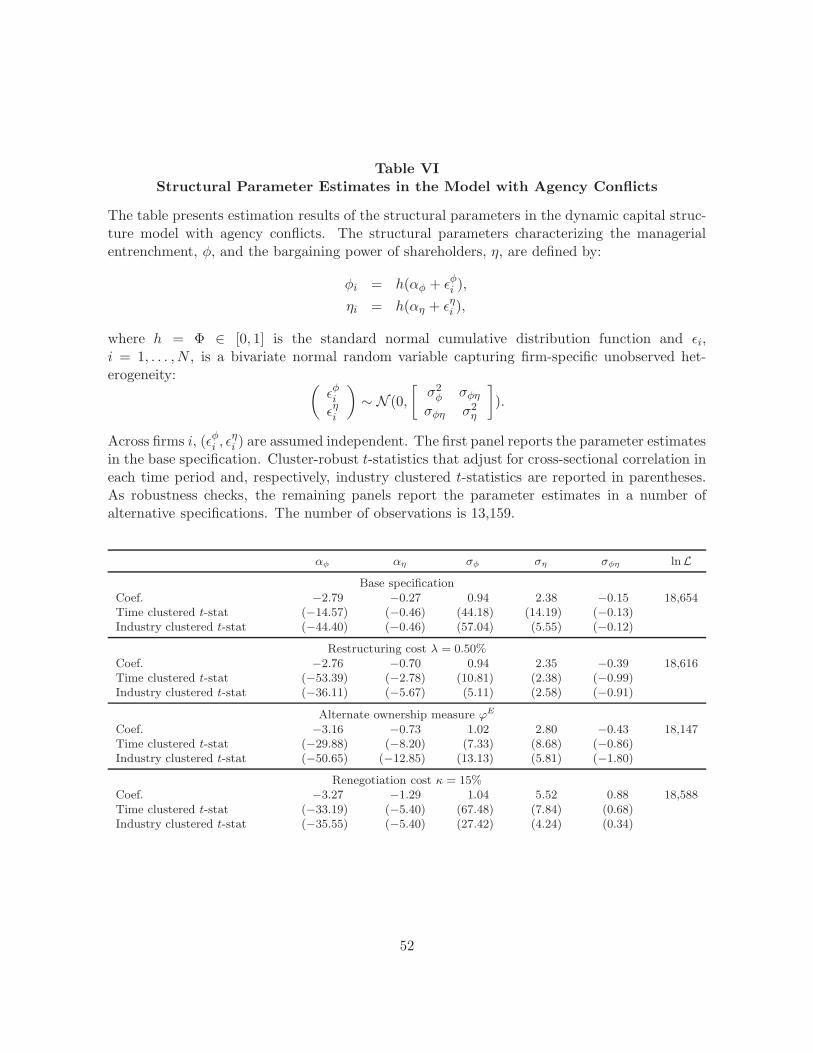
Table VI

Structural Parameter Estimates in the Model with Agency Conflicts

The table presents estimation results of the structural parameters in the dynamic capital struc-ture model with agency conflicts. The structural parameters characterizing the managerialentrenchment, φ, and the bargaining power of shareholders, η, are defined by:

φi = h(αφ + ǫφi ),

ηi = h(αη + ǫηi ),

where h = Φ ∈ [0, 1] is the standard normal cumulative distribution function and ǫi,i = 1, . . . , N , is a bivariate normal random variable capturing firm-specific unobserved het-erogeneity: (

ǫφiǫηi

)∼ N (0,

[σ2

φ σφη

σφη σ2η

]).

Across firms i, (ǫφi , ǫηi ) are assumed independent. The first panel reports the parameter estimates

in the base specification. Cluster-robust t-statistics that adjust for cross-sectional correlation ineach time period and, respectively, industry clustered t-statistics are reported in parentheses.As robustness checks, the remaining panels report the parameter estimates in a number ofalternative specifications. The number of observations is 13,159.

αφ αη σφ ση σφη lnL

Base specificationCoef. −2.79 −0.27 0.94 2.38 −0.15 18,654Time clustered t-stat (−14.57) (−0.46) (44.18) (14.19) (−0.13)Industry clustered t-stat (−44.40) (−0.46) (57.04) (5.55) (−0.12)

Restructuring cost λ = 0.50%Coef. −2.76 −0.70 0.94 2.35 −0.39 18,616Time clustered t-stat (−53.39) (−2.78) (10.81) (2.38) (−0.99)Industry clustered t-stat (−36.11) (−5.67) (5.11) (2.58) (−0.91)

Alternate ownership measure ϕE

Coef. −3.16 −0.73 1.02 2.80 −0.43 18,147Time clustered t-stat (−29.88) (−8.20) (7.33) (8.68) (−0.86)Industry clustered t-stat (−50.65) (−12.85) (13.13) (5.81) (−1.80)

Renegotiation cost κ = 15%Coef. −3.27 −1.29 1.04 5.52 0.88 18,588Time clustered t-stat (−33.19) (−5.40) (67.48) (7.84) (0.68)Industry clustered t-stat (−35.55) (−5.40) (27.42) (4.24) (0.34)

52

Table VI Continued

αφ αη σφ ση σφη lnL

Nuisance parameters set to initial value θ⋆i = θ⋆

i1

Coef. −2.83 −0.48 0.94 3.01 −0.26 18,364Time clustered t-stat (−29.70) (−0.27) (7.18) (0.48) (−0.11)Industry clustered t-stat (−21.76) (−0.41) (6.38) (0.82) (−0.13)

Nuisance parameters set to firm-time specific estimates θ⋆it

Coef. −2.98 −0.39 0.96 2.46 −0.26 -2,741Time clustered t-stat (−12.50) (−3.89) (64.66) (6.52) (−2.09)Industry clustered t-stat (−17.96) (−4.62) (114.23) (5.10) (−3.53)

Logit specification for link function hCoef. −7.16 −1.44 3.21 3.46 −1.09 18,144Time clustered t-stat (−8.88) (−1.69) (2.10) (1.66) (−0.26)Industry clustered t-stat (−12.59) (−1.96) (3.02) (2.54) (−0.68)

Alternate definition of leverageCoef. −2.24 −0.48 0.93 1.90 −0.13 -58,396Time clustered t-stat (−17.30) (−1.24) (146.15) (2.34) (−0.94)Industry clustered t-stat (−26.87) (−2.14) (185.95) (3.37) (−0.65)

53

Table VII

Managerial Entrenchment and Shareholder Bargaining Power Across Firms

The table summarizes distributional characteristics of the fitted managerial entrenchment, φi =E(φi|yi; θ), and bargaining power of shareholders, ηi = E(ηi|yi; θ), i = 1, . . . , N . Appendix A.2derives explicit expressions for φi and ηi. In brackets we report managerial entrenchmentexpressed as a fraction of equity value, E(φiF

∗i /Ei|yi; θ). The managerial entrenchment cost

estimates across firms are expressed in percent. The first panel reports the fitted values inthe base specification. As robustness checks, the remaining panels report the fitted values in anumber of alternative specifications.

Mean S.D. Skewness Kurtosis 5% 25% 50% 75% 95%

Base specification

φi 1.12 2.23 3.83 19.75 0.02 0.09 0.30 1.16 5.58[1.02] [2.23] [4.19] [23.03] [0.01] [0.07] [0.23] [0.91] [4.82]

ηi 0.43 0.25 0.01 2.08 0.03 0.23 0.46 0.61 0.85

Restructuring cost λ = 0.50%

φi 1.28 2.49 3.98 21.55 0.02 0.10 0.38 1.35 5.34[1.19] [2.50] [4.34] [25.20] [0.01] [0.09] [0.29] [1.18] [5.49]

ηi 0.39 0.23 0.38 2.45 0.04 0.22 0.38 0.54 0.83

Alternate ownership measure ϕE

φi 0.76 1.87 4.34 23.77 0.00 0.03 0.14 0.52 3.55[0.70] [1.85] [4.77] [29.03] [0.00] [0.02] [0.11] [0.47] [3.29]

ηi 0.38 0.25 0.35 2.25 0.02 0.17 0.38 0.55 0.85

Renegotiation cost κ = 15%

φi 0.86 1.96 4.32 24.81 0.01 0.05 0.16 0.72 4.38[0.77] [1.85] [4.59] [28.29] [0.01] [0.04] [0.12] [0.62] [4.00]

ηi 0.41 0.29 0.17 1.81 0.01 0.12 0.42 0.66 0.89

Nuisance parameters set to their initial value θ⋆i = θ⋆

i1

φi 1.33 2.67 3.80 19.98 0.02 0.09 0.34 1.32 6.87[1.23] [2.69] [4.19] [23.46] [0.01] [0.07] [0.27] [1.06] [6.10]

ηi 0.45 0.26 -0.02 2.02 0.03 0.23 0.46 0.66 0.88

Nuisance parameters set to firm-time specific estimates θ⋆it

φi 1.33 3.02 4.23 23.47 0.01 0.06 0.25 1.27 7.25[1.26] [3.23] [4.98] [32.54] [0.01] [0.05] [0.20] [1.04] [6.88]

ηi 0.47 0.30 0.13 1.85 0.02 0.20 0.45 0.72 0.97

Logit specification for link function h

φi 0.35 0.77 3.79 19.40 0.01 0.03 0.06 0.25 1.93[0.40] [1.03] [5.54] [46.66] [0.01] [0.02] [0.05] [0.22] [2.06]

ηi 0.30 0.19 0.54 2.80 0.04 0.14 0.29 0.41 0.65

Alternate definition of leverage

φi 3.14 5.48 3.14 13.78 0.04 0.22 0.89 4.70 15.06[3.73] [7.60] [3.78] [19.09] [0.03] [0.17] [0.66] [4.98] [17.17]

ηi 0.42 0.22 0.12 2.64 0.05 0.27 0.42 0.55 0.82

54

Table VIII

Conditional Moment Tests for Goodness-of-Fit

The table reports the results from conditional moment tests. Conditional moment (CM) testsuse conditional moment restrictions for testing goodness-of-fit. Specifically, the CM tests per-formed check whether the difference between the real data moments listed in each row and thesimulated data moments based on our SML estimates is equal to zero. We report momentsbased on both leverage levels and changes. The test statistic for each individual moment isreported in the third column next to the corresponding moment, and the associated p-value isin the last column. The Wald test statistic reported in the last row tests for joint fit of themodel by checking whether the distances between data and simulated moments are jointly zero.

Empirical Simulated CM testmoment model moment statistic p-value

Leverage:Mean 0.322 0.335 (-1.51) [0.13]Median 0.317 0.326 (-0.89) [0.37]S.D. 0.068 0.097 (-16.53) [0.00]Skew 0.220 0.354 (-6.01) [0.00]Kurtosis 2.308 2.515 (-5.31) [0.00]Range 0.216 0.297 (-14.64) [0.00]IQR 0.100 0.140 (-13.45) [0.00]Min 0.224 0.206 (3.41) [0.00]Max 0.440 0.502 (-7.27) [0.00]Autocorrelation 1qtr 0.916 0.882 (0.70) [0.49]Autocorrelation 1yr 0.737 0.602 (2.74) [0.01]

Changes in leverage:Mean 0.005 0.001 (4.95) [0.00]Median 0.003 0.001 (1.72) [0.09]S.D. 0.049 0.110 (-50.63) [0.00]Skewness 0.258 0.013 (8.96) [0.00]Kurtosis 3.071 3.135 (-1.03) [0.30]Range 0.058 0.132 (-48.81) [0.00]IQR -0.076 -0.189 (45.06) [0.00]Min 0.100 0.192 (-33.79) [0.00]Max 0.176 0.381 (-46.44) [0.00]Autocorrelation 1qtr -0.090 -0.035 (-1.45) [0.15]Autocorrelation 1yr -0.033 -0.059 (0.67) [0.50]

Wald test of joint hypothesis H0: All moments equal (0.49) [1.00]

55

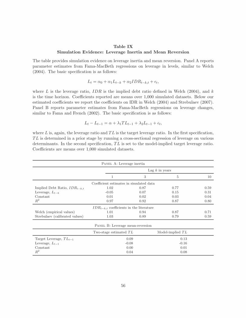
Table IX

Simulation Evidence: Leverage Inertia and Mean Reversion

The table provides simulation evidence on leverage inertia and mean reversion. Panel A reportsparameter estimates from Fama-MacBeth regressions on leverage in levels, similar to Welch(2004). The basic specification is as follows:

Lt = α0 + α1Lt−k + α2IDRt−k,t + ǫt,

where L is the leverage ratio, IDR is the implied debt ratio defined in Welch (2004), and kis the time horizon. Coefficients reported are means over 1,000 simulated datasets. Below ourestimated coefficients we report the coefficients on IDR in Welch (2004) and Strebulaev (2007).Panel B reports parameter estimates from Fama-MacBeth regressions on leverage changes,similar to Fama and French (2002). The basic specification is as follows:

Lt − Lt−1 = α+ λ1TLt−1 + λ2Lt−1 + ǫt,

where L is, again, the leverage ratio and TL is the target leverage ratio. In the first specification,TL is determined in a prior stage by running a cross-sectional regression of leverage on variousdeterminants. In the second specification, TL is set to the model-implied target leverage ratio.Coefficients are means over 1,000 simulated datasets.

Panel A: Leverage inertia

Lag k in years

1 3 5 10

Coefficient estimates in simulated dataImplied Debt Ratio, IDRt−k,t 1.02 0.87 0.77 0.59Leverage, Lt−k -0.05 0.07 0.15 0.31Constant 0.01 0.02 0.03 0.04R2 0.97 0.92 0.87 0.80

IDRt−k,t coefficients in the literatureWelch (empirical values) 1.01 0.94 0.87 0.71Strebulaev (calibrated values) 1.03 0.89 0.79 0.59

Panel B: Leverage mean-reversion

Two-stage estimated TL Model-implied TL

Target Leverage, TLt−1 0.09 0.13Leverage, Lt−1 -0.08 -0.16Constant 0.00 0.01R2 0.04 0.08

56

Table X

Specification Analysis

The table reports likelihood ratio tests to select the best model amongst alternative model spec-ifications. We report test statistics for nested and non-nested models as derived in Appendix E.In addition to the base specification given in (14) and (15), we consider six additional nestedmodels and two non-nested models: (1) φi and ηi, i = 1, . . . , N , with uncorrelated random

effects (φi = h(αφ + ǫφi ), ηi = h(αη + ǫηi ), σφη = 0), (2) no shareholder bargaining power

(φi = h(αφ + ǫφi ), ηi = 0), (3) no managerial entrenchment (φi = 0, ηi = h(αη + ǫηi )), (4) φand η constant (φi = h(αφ), ηi = h(αη)), (5) no shareholder bargaining power and φ constant(φi = h(αφ), ηi = 0), (6) no managerial entrenchment and η constant (φi = 0, ηi = h(αη)), andthe two non-nested models (7) λ with random effects (λi = h(αλ + ǫλi ), φi = 0, ηi = 0), (8) λconstant (λi = h(αλ), φi = 0, ηi = 0). Tests for non-nested models are based on Vuong (1989)and indicated by †. p-values are reported in brackets. For the nested models, a p-value of zeroindicates that the null hypothesis that the parameter restrictions are valid is rejected in favorof the model under the alternative. For the non-nested models, a p-value of zero indicates thatthe null hypothesis that the two models are equivalent is rejected in favor of the model underthe alternative.

Alternative Null hypothesis

hypothesis (1) (2) (3) (4) (5) (6) (7) (8)

Base 1,423 6,864 256,001 214,771 209,506 351,529 2.72† 19.60†

[0.00] [0.00] [0.00] [0.00] [0.00] [0.00] [0.00] [0.00]

(1) – 5,441 254,578 213,348 208,083 350,106 1.80† 19.51†

– [0.00] [0.00] [0.00] [0.00] [0.00] [0.04] [0.00]

(2) – – 16.75† 15.22† 202,641 21.68† -1.13† 19.24†

– – [0.00] [0.00] [0.00] [0.00] [0.87] [0.00]

(3) – – – -3.43† -3.71† 95,529 -17.28† 3.30†

– – – [1.00] [1.00] [0.00] [1.00] [0.00]

(4) – – – – -5,265 136,759 -15.27† 5.73†

– – – – [1.00] [0.00] [1.00] [0.00]

(5) – – – – – 10.63† -15.43† 5.99†

– – – – – [0.00] [1.00] [0.00]

(6) – – – – – – -21.92† -1.02†

– – – – – – [1.00] [0.85](7) – – – – – – – 324,602

[0.00]

57

Table XI

The Determinants of Managerial Entrenchment

The table summarizes the determinants of the managerial entrenchment across firms. Thedependent variable is the predicted value of managerial entrenchment, φi = E(φi|yi; θ) fori = 1, . . . , N , where θ are the parameters estimated in Section III.B and the φi are expressedin basis points. In columns (1)-(3) we report estimation results from cross-sectional regres-sions. Specification (1) utilizes the entire sample. Missing values are imputed with zero anddummy variables that take a value of one for missing values are included in the regression.Specifications (2) and (3) use only observations with no missing data items. In specification(2) we drop the variables with the most missing values from the regression. All specificationsare estimated including industry fixed effects. Standard errors are adjusted for sampling errorin the generated regressands (see Handbook of Econometrics IV, p. 2183) and are reported inparentheses. Statistical significance at the 10%, 5% and 1% level is marked with *, **, and ***,respectively.

(1) (2) (3)

Institutional Ownership −88.15** −90.72*** −66.24*(37.79) (34.67) (37.90)

Independent Blockholder Ownership −74.73 −95.37** −99.98**(52.06) (47.52) (49.70)

E-index - Dictatorship 172.72** 137.92* 133.73*(68.84) (75.68) (76.81)

CEO Tenure 3.72*** 4.70*** 4.85***(1.02) (1.15) (1.30)

Board Independence −78.19* − −72.03(40.04) − (45.85)

Board Committees −6.58 − −3.78(6.99) − (6.89)

Managerial Delta (Quartile 1) −8.68 −14.82 −12.22(11.97) (12.10) (11.80)

Managerial Delta (Quartile 4) 3.21*** 3.39*** 3.45***(0.78) (0.81) (0.94)

Returns on Assets 0.95 1.08 −0.38*(4.04) (4.24) (4.92)

M/B 38.11*** 33.28*** 29.84**(9.00) (11.31) (12.22)

Asset Tangibility −25.23 14.23 26.81(34.69) (37.73) (39.37)

Size −39.47*** −39.04*** −39.36***(6.08) (5.97) (6.62)

R&D 1.16 0.35 4.98(8.44) (10.31) (10.27)

Observations 809 634 569R2 0.35 0.35 0.37

58

Figure 1

Monte-Carlo Simulation Precision and Accuracy

The figure depicts the magnitude of Monte-Carlo simulation error and its impact on the precision and

accuracy of the simulated log-likelihood. In all plots, on the horizontal axis we vary the number of

random draws K used to evaluate the log-likelihood. For given K, we evaluate the log-likelihood 100

times at the same parameters and in each round vary the set of random numbers used to integrate

out the firm-specific random effects from the likelihood function. Panel A reports box plots for the

simulated values of the log-likelihood across simulation rounds. Depicted are the lower quartile, median,

and upper quartile values as the lines of the box. Whiskers indicate the adjacent values in the data.

Outliers are displayed with a + sign. The highest simulated log-likelihood value across all simulation

rounds is indicated by a dotted line. Panel B depicts the magnitude of the simulation imprecision (left)

and the simulation bias (right) as function of K. The simulation imprecision is measured by the 95%

quantile minus the 5% quantile across all simulation rounds for given K and normalized by the highest

simulated log-likelihood value across all simulation rounds. The simulation bias is measured by the

median log-likelihood value across all simulation rounds for given K relative to the highest simulated

log-likelihood value across all simulation rounds.

Panel A: Simulated values of the log-likelihood

2 3 4 5 10 25 50 100 250 500 750 1000

−8

−6

−4

−2

0

2

x 104

Sim

ulat

ed lo

g−lik

elih

ood

K

Panel B: Simulation precision and accuracy of the simulated log-likelihood

2 3 4 5 10 25 50 100 250 500 750 1000

100

101

102

Sim

ulat

ion

impr

ecis

ion

(%)

K2 3 4 5 10 25 50 100 250 500 750 1000

100

101

102

103

Sim

ulat

ion

bias

(%

)

K59

Figure 2

Comparative Statics: Firm-Specific Leverage Distribution

The figure shows comparative statics for the time-series distribution of financial leverage. We vary the refinancing cost λ, the degree of

managerial entrenchment φ, and shareholders’ bargaining power η around the baseline values (λ, φ, η) = (.005, .005, .25). Panel A plots the

distribution function of leverage for different parameter values. Panel B depicts the median (solid line), the 5% and 95% quantiles of leverage

(dashed lines), and the low and high of leverage (dotted lines) as functions of the parameters.

Panel A: Leverage density function under alternative parameter values

0 0.2 0.4 0.6 0.8 10

1

2

3

4

5

Leverage

Den

sity

λ = 0.5%λ = 5%

0 0.2 0.4 0.6 0.8 10

1

2

3

4

5

LeverageD

ensi

ty

φ = 0.5%

φ = 1.5%

0 0.2 0.4 0.6 0.8 10

1

2

3

4

5

Leverage

Den

sity η = 25%

η = 75%

Panel B: Moments of leverage distribution as function of parameter values

0 0.05 0.1 0.150

0.2

0.4

0.6

0.8

1

Leve

rage

λ0 0.01 0.02

0

0.2

0.4

0.6

0.8

1

Leve

rage

φ0 0.5 1

0

0.2

0.4

0.6

0.8

1

Leve

rage

η

60

Figure 3

Managerial Entrenchment and Shareholder Bargaining Power Across Firms

The figure shows histograms of the predicted managerial entrenchment, E(φi|yi, xi; θ), and the predicted

shareholders’ bargaining power, E(ηi|yi, xi; θ), for firms i = 1, . . . , N in the dynamic capital structure

model. The prediction is based on a structural estimate of the model’s parameters. The histograms plot

the predicted parameters for each firm-quarter.

Panel A: Distribution of predicted managerial entrenchment φi

0 1 2 3 4 50

100

200

300

400

Managerial entrenchment (%)

Fre

quen

cy

Panel B: Distribution of predicted shareholder bargaining power ηi

0 20 40 60 80 1000

20

40

60

80

100

Shareholder bargaining power (%)

Fre

quen

cy

61