Corporate cash shortfalls and financing decisions · 2016-05-25 · Corporate cash shortfalls and...
63
Corporate cash shortfalls and financing decisions Rongbing Huang and Jay R. Ritter * December 5, 2015 Abstract Immediate cash needs are the primary motive for debt issuances and a highly important motive for equity issuances. A two standard deviation increase in free cash flow-to-assets on average decreases the likelihood of a net debt issue and a net equity issue in the same year by 53.6% (from 60.0% to 6.4%) and 12.7% (from 18.4% to 5.7%), respectively. Conditional on issuing a security, corporate lifecycle, precautionary saving, market timing, and static tradeoff theories are important in explaining the debt versus equity choice, even for firms that are running out of cash. Key Words: Cash Holding, Cash Need, Equity Issue, Debt Issue, Security Issue, SEO, Financing Decision, Capital Structure, Market Timing, Precautionary Saving, Corporate Lifecycle, Financial Flexibility, Static Tradeoff JEL: G32 G14 * Huang is from the Coles College of Business, Kennesaw State University, Kennesaw, GA 30144. Huang can be reached at [email protected]. Ritter is from the Warrington College of Business Administration, University of Florida, Gainesville, FL 32611. Ritter can be reached at [email protected]. We would like to give special thanks to our referee for detailed and highly constructive comments. We also thank Ning Gao (our FMA discussant) and the participants at the University of Sussex, Tsinghua PBC, the Harbin Institute of Technology, and the 2015 FMA Annual Meeting for useful comments.
Transcript of Corporate cash shortfalls and financing decisions · 2016-05-25 · Corporate cash shortfalls and...

Corporate cash shortfalls and financing decisions
Rongbing Huang and Jay R. Ritter∗
December 5, 2015
Abstract
Immediate cash needs are the primary motive for debt issuances and a highly important motive
for equity issuances. A two standard deviation increase in free cash flow-to-assets on average
decreases the likelihood of a net debt issue and a net equity issue in the same year by 53.6%
(from 60.0% to 6.4%) and 12.7% (from 18.4% to 5.7%), respectively. Conditional on issuing a
security, corporate lifecycle, precautionary saving, market timing, and static tradeoff theories are
important in explaining the debt versus equity choice, even for firms that are running out of cash.
Key Words: Cash Holding, Cash Need, Equity Issue, Debt Issue, Security Issue, SEO, Financing Decision, Capital Structure, Market Timing, Precautionary Saving, Corporate Lifecycle, Financial Flexibility, Static Tradeoff JEL: G32 G14
∗ Huang is from the Coles College of Business, Kennesaw State University, Kennesaw, GA 30144. Huang can be reached at [email protected]. Ritter is from the Warrington College of Business Administration, University of Florida, Gainesville, FL 32611. Ritter can be reached at [email protected]. We would like to give special thanks to our referee for detailed and highly constructive comments. We also thank Ning Gao (our FMA discussant) and the participants at the University of Sussex, Tsinghua PBC, the Harbin Institute of Technology, and the 2015 FMA Annual Meeting for useful comments.
1
1. Introduction
Firms issue securities to fund immediate cash needs, optimize cash holdings, prepare for
future cash needs, rebalance capital structures, time the market, or achieve other goals.1 In this
paper, we examine the economic significance of cash needs and non-funding-related factors in
predicting debt or equity issue decisions of U.S. firms during 1972-2010. Our findings suggest
that immediate cash needs are the primary determinant of the decision to raise external capital,
especially debt, and that corporate lifecycle, precautionary saving, market timing, and static
tradeoff motives are important for the choice between debt and equity.
We find that immediate cash needs are the dominant predictor for debt issues.2 After
controlling for other variables, a two standard deviation increase in the ratio of free cash flow-to-
beginning of year assets on average decreases the likelihood of a net debt issue in the same fiscal
year by 53.6% (from 60.0% to 6.4%). Net debt issuers spend 85.9 cents of each dollar raised in
the same year. These findings strongly support the transitory debt theory developed by DeAngelo,
DeAngelo, and Whited (2011). The theory posits that firms deliberately but temporarily deviate
from permanent target leverage by issuing transitory debt to fund investments.
We also find that immediate cash needs are a highly important motive for equity issues.
A two standard deviation increase in free cash flow-to-assets for a year on average decreases the
likelihood of a net equity issue in the same year by 12.7% (from 18.4% to 5.7%). Net equity
issuers immediately spend 34.6 cents of each dollar raised. Cash balance optimization, future
needs, corporate lifecycle, and precautionary saving proxies can explain saving 17.9 cents of
1 See Myers (1984), Loughran and Ritter (1995), Hovakimian, Opler, and Titman (2001), Baker and Wurgler (2002), Frank and Goyal (2003), Welch (2004), Fama and French (2005), Leary and Roberts (2005), Huang and Ritter (2009), DeAngelo, DeAngelo, and Stulz (2010), Billett, Flannery, and Garfinkel (2011), and DeAngelo and Roll (2015), among others. 2 In this paper, we use “immediate cash need” to denote year t cash need, “near-future” to denote year t+1, “near-term” to denote both t and t+1, and “remote-future” or “remote” to denote t+2 and later.

2
each dollar raised. Market timing proxies can explain a saving of 9.2 cents, with the remaining
38.3 cents unexplained.
We document that firms behave much like individuals: they rarely raise external capital
unless there is an immediate cash need. When there is an immediate cash need, firms can choose
to issue debt or equity to fund it. Conditional on issuing a security, our proxies for corporate
lifecycle, precautionary saving, market timing, and tradeoff theories are important in explaining
the debt versus equity choice, even for firms that are running out of cash.
The corporate lifecycle theory posits that young firms rely more on external equity than
old firms (DeAngelo, DeAngelo, and Stulz (2010), henceforth DDS). The precautionary saving
theory posits that firms facing more uncertainties are more likely to issue equity rather than debt
and prefer higher cash balances (Bates, Kahle, and Stulz (2009) and McLean (2011)). The static
tradeoff theory emphasizes adjustment toward leverage targets. The market timing theory posits
that firms issue equity when the relative cost of equity is low and issue debt when the relative
cost of debt is low. Three versions of timing theories appear in the literature. Unconditional
timing theories view market timing as important and economic fundamentals (e.g., funding needs
as well as lifecycle, precautionary saving, and tradeoff motives) as unimportant or negligible for
securities issuance decisions. Conditional timing theories recognize the importance of both
market timing and fundamentals. Reverse-causality timing theories emphasize causality that runs
from timing opportunities to real decisions (Baker, Stein, and Wurgler (2003)). Specifically,
when the cost of capital is low, firms raise capital and quickly spend the proceeds on projects
that they would not otherwise take. Our findings are consistent with conditional timing theories.
Recently, the economic importance of explicit measures of near-term cash needs as a
motivation for securities issuances has started to receive much-deserved attention. In an
3
influential paper, DDS find that 62.6% of the firms conducting seasoned equity offerings (SEOs)
would have run out of cash at the end of the year after the SEO without the proceeds. DDS also
document that many mature firms conduct an SEO, and many firms with good equity market
timing opportunities do not conduct an SEO. They thus conclude that neither lifecycle nor timing
is sufficient in explaining SEO decisions. DDS also find that the likelihood of an SEO is much
higher for young firms than for old firms, suggesting that the lifecycle effect is more important
than the timing effect. Taking their findings together, DDS conclude that near-term cash needs
are the primary motive for SEOs.
In another important paper that explicitly measures an immediate cash need, Denis and
McKeon (2012) document that debt issues accompanied by large leverage increases are primarily
used to fund immediate operating needs, and that there is little attempt to subsequently reduce
the debt ratio, inconsistent with the static tradeoff model.
Kim and Weisbach (2008) find that firms save 53.4 cents of an incremental dollar raised
in an SEO, suggesting a timing-related stockpiling effect. Using Compustat data to define equity
issues, McLean (2011) shows in his Table 6 that one additional dollar of equity issuance results
in 56.4 cents of cash savings. McLean concludes that precautionary saving motives are important
for equity issuances. His Table 11 documents that the likelihood of cash depletion in a year is 17%
for firms that report a positive equity issue amount on their cash flow statements, in sharp
contrast with the cash depletion likelihood of 62.6% for SEOs that DDS report. The difference
between their findings is largely because McLean’s sample includes many small equity issues
attributable to the exercise of employee stock options for firms without large investment needs.
Our paper differs from the previous papers in four major regards. First, we evaluate the
relative economic significance of current cash needs, future cash needs, and non-funding-related

4
factors in explaining debt and equity issue decisions. Second, we relate cash changes associated
with securities issues to cash needs, and precautionary, timing, lifecycle, and other motives.
Third, we evaluate the importance of various theories in explaining the choice between debt and
equity, conditional on issuing a security. In contrast, Kim and Weisbach (2008), DDS, and
McLean (2011) only focus on equity issues, while Denis and McKeon (2012) only focus on debt
issues. Lewis and Tan (2015) focus on the ability of the debt vs. equity choice to predict future
stock returns, but do not address motivations for financing decisions other than market timing.
Finally, we reconcile some of the disparate results in the previous papers.
In this paper, we define securities issues using information from cash flow statements. A
firm is defined as a debt issuer or an equity issuer if net debt or net equity proceeds in a year are
at least 5% of the book value of assets and 3% of the market value of equity at the beginning of
the year. In our definition, equity issues include SEOs, private investments in public equity
(PIPEs), large employee stock option exercises, and preferred stock issues.3 One argument
against the market timing theory is that many firms with good equity market timing opportunities
do not issue equity. In our sample, an equity issue occurs in 10.7% of the firm-years. In
comparison, DDS document that the probability of an SEO in a given year is 3.4%.4 Debt issues
in our sample include straight and convertible bond offerings and increases in bank loans.
Our findings on the likelihood of cash depletion are generally consistent with those of
DDS, although we also document that many equity issuers would not run out of cash even if they
cut their issue size by half. Of the equity issuers in our sample, 54.4% would run out of cash at
3 Since we require a one-year stock return prior to the current fiscal year, initial public offerings (IPOs) and SEOs shortly after the IPO are not included in our sample. Because cash flow statements are used, stock-financed acquisitions are not counted as equity issues in this paper. 4 To understand why our frequency of equity issues is so much higher than the DDS frequency, we investigated 50 random equity issuers using the Thomson Reuters’ SDC database, Sagient Research’s Placement Tracker database, and annual reports on the S.E.C.’s EDGAR web site. We found that PIPEs were almost as frequent as SEOs, and that SDC missed some SEOs.

5
the end of the issuing year if they did not raise capital, and 34.7% would run out of cash if they
cut the net equity and net debt issue size by half.
We use two variables to explicitly measure immediate cash needs: cash at the end of year
t-1, Casht-1, and free cash flow in year t, FCFt. We define FCF in a year as ICF – Investments –
∆Non-Cash NWC – Cash Dividends, where ICF is the internal cash flow, and ∆Non-Cash NWC
is the change in non-cash net working capital (see the Appendix for details). We use FCFt+1 and
FCFt+2, respectively, to measure near-future and remote-future cash needs. Note that higher
Casht-1 and FCF reflect a larger cash surplus or a smaller cash need. All of these cash need
variables are scaled by the book value of assets at the end of t-1, Assetst-1.
We estimate multinomial logit regressions to evaluate the economic significance of
various determinants for the decision to issue debt, equity, both debt and equity, or no security.5
Immediate cash needs are the dominant determinant for debt issuances. Simply put, firms do not
borrow money unless they are going to spend it. Near-future cash needs are much less important
than immediate cash needs, and lagged leverage and remote-future cash needs have negligible
predictive power for debt issues. These findings provide strong support for the transitory debt
theory developed in DeAngelo, DeAngelo, and Whited (2011).
Immediate cash needs are also highly important for equity issues. A two standard
deviation increase in Casht-1 ÷Assetst-1 or FCFt ÷Assetst-1 decreases the likelihood of a net equity
issue by 5.0% (from 13.8% to 8.8%) and 12.7% (from 18.4% to 5.7%), respectively. Future cash
needs are also important but less important than immediate cash needs. A two standard deviation
5 Hovakimian (2004) does not evaluate the economic effects of the independent variables in his multinomial logit regressions and does not focus on the role of cash needs. Huang and Ritter (2009) do not explicitly control for cash needs in their nested logit regressions. DDS do not examine the choice between debt and equity and do not include a cash shortfall measure as an independent variable in their logit regressions for the decision to conduct an SEO. Denis and McKeon (2012) focus on debt issues associated with large leverage increases, and do not examine the decision to issue debt.

6
increase in FCFt+1 ÷Assetst-1 and FCFt+2 ÷ Assetst-1 decreases the likelihood of a net equity issue
in year t by 4.3% and 2.2%, respectively.
Larger and older firms, firms with higher stock returns from year t+1 to t+3 (a measure of
current undervaluation), and dividend payers are less likely to issue equity. The stock return in
year t-1, Tobin’s Q, leverage, R&D expense, and industry cash flow volatility are positively
associated with the likelihood of equity issues. Firms are also more likely to issue equity when
the default spread is high. These findings are consistent with lifecycle, timing, precautionary
saving, and tradeoff theories.
Our current and future free cash flow measures are based on actual internal cash flow and
cash uses. Reverse-causality timing theories posit that firms spend more only because they
successfully raise external capital. To avoid this reverse causality concern, we also use an ex ante
measure of free cash flow, FCFt-1. Impressively, Casht-1 ÷ Assetst-1 and FCFt-1 ÷ Assetst-1 are still
the most important determinants of debt issues and important determinants for equity issues. For
equity issues, the economic significance of FCFt-1 ÷ Assetst-1 is comparable to that of firm size or
that of the stock return from t+1 to t+3.
We also examine the effects of debt and equity issues on cash changes, and how the
effects are related to cash needs and non-funding-related motives. On average, net debt issuers
immediately spend 85.9 cents of an incremental dollar in their issuing proceeds, and save only
14.1 cents in cash. In comparison, net equity issuers immediately spend 34.6 cents of an
incremental dollar in their issuing proceeds, and save 65.4 cents in cash. The fact that equity
issuers tend to save a large fraction of issue proceeds has been interpreted as supportive of the
market timing theory (Kim and Weisbach (2008)). We caution that timing is not responsible for
all of the 65.4 cents saving. As DDS also note, many equity issuers are small and unprofitable

7
and experience substantial growth in non-cash assets, thus it is reasonable for them to increase
cash balances and prepare for future cash needs.
To understand the relative importance of various motives for cash savings, we
decompose the saving of 65.4 cents into three components. Fundamentals can justify a cash
increase of 17.9 cents of an incremental dollar in net equity issue proceeds. Firms with non-cash
asset growth and larger potential future financing needs, smaller firms, and firms facing more
uncertainties generally save more in cash. After controlling for the effects of the fundamentals,
market timing proxies can explain a saving of 9.2 cents, with more saved when equity is cheap.
The saving explained by timing proxies is smaller than that explained by fundamentals,
suggesting that although timing is important, fundamentals are even more important. A saving of
38.3 cents remains unexplained.
Immediate cash needs are not incompatible with market timing and other motives. Firms
that are running out of cash still must choose between debt and equity if they seek external
financing. Conditional on issuing a security, firms with smaller immediate cash needs and larger
future cash needs are more likely to issue equity rather than debt. Other than cash needs, the four
most important predictors of the debt vs. equity choice are lagged measures of firm size, R&D
expense, leverage, and Tobin’s Q. A two standard deviation increase in lagged firm size is
associated with a decrease of 12.5% in the likelihood of equity issues, and a two standard
deviation increase in lagged R&D expense, leverage, and Tobin’s Q is associated with increases
in the equity issue likelihood of 10.5%, 8.0%, and 7.9%, respectively.
We further estimate a multinomial logit regression for the choice of securities,
conditional on doing external financing and running out of cash. Even for firms that are running
out of cash, market timing, precautionary savings, corporate lifecycle, and tradeoff theories are
8
economically important in explaining the debt versus equity choice. Companies usually raise
cash only when they need to, but if a firm is small, young, R&D intensive, highly levered, or if
equity is cheap, the firm will frequently issue equity rather than debt.
2. Data, variables, and summary statistics
2.1. Data and variables
We use Compustat to obtain financial statement information and CRSP to obtain stock
prices for each U.S. firm. We require the statement of cash flow information for fiscal years t and
t-1. Since the cash flow information is only available from 1971, our final sample starts from
1972.6 Since we also examine stock returns in the three years after each financing decision, our
sample period ends at 2010. We also drop firm-year observations for which frequently used
variables in our paper have a missing value, the net sales is not positive, the book value of assets
at the end of fiscal year t-1 or t is less than $10 million (expressed in terms of purchasing power
at the end of 2010), the book value of assets at the end of year t-2 is missing, the cash flow
identity is violated, or there is a major merger.7 To avoid the effect of regulations on financing
choices, we remove financial and utility firms from our analysis. Our final sample includes
116,488 firm-year observations from 1972-2010.
As market timing proxies we use Tobin’s Q, the stock return in year t-1, the stock return
from t+1 to t+3, the term spread, and the default spread. As lifecycle proxies, while DDS use
only firm age, we favor the corporate lifecycle theory by using both firm size (the logarithm of
6 We use the number of years that a firm has been listed on CRSP as a measure for the firm’s age. CRSP first included NASDAQ stocks in December 1972. As DDS point out, the number of years on CRSP is not a reliable measure for firm age for these firms. Our major results are essentially the same if we add five years to the age of these firms or simply exclude these firms from our sample. 7 A major merger is identified by the Compustat footnote for net sales being AB, FD, FE, or FF. Our data requirements result in the dropping of firms that solved their cash shortfall problems by being acquired during year t.

9
net sales) and age. As precautionary saving proxies, following McLean (2011), we use R&D
expense, industry cash flow volatility, and a dividend payer dummy variable. For the tradeoff
theory, we use lagged leverage as a proxy. Detailed definitions of the variables used in this paper
are provided in the Appendix. To minimize the influence of outliers, all non-categorical variables
except for the stock returns are winsorized at the 0.5% level at each tail of our sample.
2.2. Summary statistics
Figure 1A reports the likelihood of cash depletion on the basis of Cash ex post, defined as
Casht-1 + FCFt. Inspection of the figure shows that larger issue sizes are associated with a higher
probability of running out of cash. Furthermore, this relation is much stronger for debt issues
than equity issues. The finding that firms that raise more debt or equity capital often have larger
cash needs undercuts the importance of precautionary saving and unconditional market timing
motives. Figure 1B shows the likelihood of cash depletion on the basis of Cash ex ante, defined as
Casht-1 + FCFt-1. Cash ex ante is fully ex ante because it only uses information prior to year t. It
assumes that the ICF, investments, ∆Non-Cash NWC, and cash dividends in year t will stay the
same as those in year t-1. There is still a positive relation between issue size and the likelihood of
cash depletion in Figure 1B, although the relation is weaker than in Figure 1A. For firms with an
issue size greater than 5% of beginning-of-year assets, the cash depletion likelihoods on the basis
of Cash ex ante are lower than those on the basis of Cash ex post for both debt and equity issuers.
Table 1 reports the sample distribution by security issue activities. If firms actively target
a desired capital structure, firms with the largest cash shortfalls could issue both debt and equity
to fund their cash needs and stay close to their target leverage (Hovakimian, Hovakimian, and
Tehranian (2004)). Therefore, we distinguish among pure debt issues, pure equity issues, and
dual issues of both debt and equity.

10
In this paper, issuance years are defined as years in which either the net debt or net
equity proceeds on the cash flow statement is at least 5% of book assets and 3% of market equity
at the beginning of the year. Using this definition, in 70.7% of firm-years, there is no security
issue. A debt issue occurs more often than an equity issue. A pure debt issue occurs in 18.7% of
firm-years, a pure equity issue occurs in 8.0% of firm-years, and dual issues of debt and equity
occur in 2.7% of firm-years. An equity issue occurs in 10.7% of firm-years in our sample. In
comparison, DDS document that the probability of an SEO in a given year is 3.4%.8
Conditional on issuing at least one security, the likelihoods of a debt issue and an equity
issue are 72.7% and 36.4%, respectively. Conditional on issuing at least one security and running
out of cash at the end of year t without external financing, the likelihoods of a debt issue and an
equity issue are 82.5% and 29.5%, respectively. Among issuers that are not running out of cash,
the likelihood of an equity issue is much higher at 50.5%. In other words, firms almost never
borrow until the money is needed, but they sometimes issue equity before it is needed.
Figure 2 shows for each fiscal year of 1972-2010 the fraction of debt or equity issuers
that have an equity issue in the year and the average Tobin’s Q at the end of the year. The
fraction varies substantially between the minimum of 5% in 1974 and the maximum of 65% in
2009. Part of the variation in the equity versus debt choice from year-to-year is undoubtedly due
to a changing composition of firms. To understand whether time-varying growth opportunities
and costs of equity help explain the variation in the debt versus equity choice across time, we
8 Fama and French (2005) document that although SEOs are rare, on average 54% of their sample firms make net equity issues each year from 1973-1982, and the proportion increases to 62% for 1983-1992 and 72% for 1993-2002. Our equity issue probabilities are lower than those reported in Fama and French (2005), who do not impose a minimum requirement of 5% of assets and 3% of market equity, and who include share issues that do not generate cash, such as stock-financed acquisitions and contributions to employee stock ownership plans (ESOPs). Although exercises of employee stock options generate cash for the company, they are passive, rather than active, actions by the issuing firm, and they occur following stock price increases, although not necessarily after an increase in t-1. McKeon (2015) reports that a 3% of market equity screen removes from the equity issuance category almost all firm-years with only stock option exercises.

11
plot the average Tobin’s Q of our sample firms at the end of each year in the same figure. The
large variation over time in the choice of debt versus equity as well as the strong positive
correlation between the fraction of issuers that issue equity and the average Tobin’s Q suggest
that market timing is quantitatively very important.
Panel A of Table 2 reports the means for the components of cash flows. On average, pure
equity issuers and dual issuers have the lowest ICFt ÷Assetst-1, suggesting that they are less able
to rely on internally generated funds. Dual issuers have the largest Investmentst ÷Assetst-1,
followed by pure debt issuers and pure equity issuers. The mean of Cash Dividendst ÷Assetst-1 is
no greater than 1.2% for all four categories of firms, suggesting that dividend cuts and omissions
play a limited role in meeting large short-term cash needs. The overall mean of 1.1% is low
because we are equally weighting firms, and most small firms pay no dividends. The mean
∆NWCt ÷ Assetst-1 varies from 0.3% for firms that issue no security to 17.9% for dual issuers.
Panel B of Table 2 reports the mean free cash flows from year t-1 to t+2. For pure debt
issuers, FCF dips in year t. FCF ÷ Assetst-1 sharply decreases from -5.3% in t-1 to -16.7% in t,
before rebounding to -6.5% and -5.7% in t+1 and t+2, respectively. In contrast, for pure equity
issuers, FCF÷ Assetst-1 decreases from -15.7% in t-1 to -18.5% in t, and decreases further to -
22.7% and -22.1% in t+1 and t+2, respectively, suggesting that equity issuers have persistently
larger funding needs. Panel B also reports the percent of firms that have a negative free cash flow.
The patterns are similar to the patterns for the means.
Our Figure 1 finds that firms that have a larger issue are more likely to run out of cash if
they do not issue. To further understand this finding, Panels C and D of Table 2 report the means
of the cash flow components for firms sorted by net equity issue size and net debt issue size,
respectively, as a percent of beginning-of-year assets. Consistent with our conjecture, firms with
12
a larger ∆Equityt ÷Assetst-1 generally have larger investments. Furthermore, for firms with
∆Equityt ÷Assetst-1≥0.05, ICFt ÷Assetst-1 is only 1.2%. Thus, part of the issue proceeds for this
group of firms is used to make up for the lower profitability. Interestingly, this group of firms not
only has the largest cash need, but also has the largest increase in cash holdings in the same year.
So a higher likelihood of cash depletion without the issuance is not necessarily incompatible with
an increase in cash holdings in the same year. In other words, corporate cash savings can and
does occur when the security issuer would have run out of cash without the issue proceeds.
When firms do issue equity, they could raise more equity capital than their immediate cash needs,
saving some to finance future cash needs. Firms with a larger ∆Debtt ÷Assetst-1 have larger
Investmentst ÷Assetst-1, although ICFt ÷Assetst-1 is flat across the debt issue size groups.
Firms could fund their uses of cash by using previously accumulated cash. Table 3
reports the summary statistics for cash, excess cash (i.e., industry-adjusted), and hypothetical
likelihoods of cash depletion. Panel A reports the means of cash and excess cash at the end of
each year from t-1 to t+1, all expressed as a percent of assets at the end of t-1. Pure equity issuers
have much higher mean cash ratios in the year before, the year of, and the year after the issue
than the other categories of firms, suggesting a stockpiling effect.
A higher cash ratio can be optimal for small growth firms, as noted by DDS. For example,
a biotech company with negative ICF will find it easier to attract and retain employees if it has
cash on the balance sheet. To control for the effects of industry, growth opportunities, and firm
size, we compute the excess cash ratios as the difference between the cash ratio of the firm and
the median cash ratio in the same year of firms in the same industry, the same tercile of Tobin’s
Q, and the same tercile of total assets. In Panel A of Table 3, pure equity issuers have a positive
mean excess cash ratio of 2.5% at the end of year t-1, but still choose to raise more equity capital.
13
To measure the likelihood of cash depletion of an SEO firm, DDS initially focus on an ex
post measure of the issuer’s pro forma cash balance at the end of the subsequent fiscal year (t+1)
after the SEO year (t), assuming zero SEO proceeds in year t and that the firm’s actual operating,
investing, and other financing activities in t and t+1 would be the same whether or not the firm
had the SEO in year t. To alleviate potential reverse-causality concerns, they do a robustness test
by assuming no capital expenditure increases in t and t+1, no increases in debt in t and t+1, or no
dividends in t and t+1, and still find that most SEO issuers would have run out of cash.
Following DDS, we present the likelihoods of cash depletion in Panel B. On the basis of
the ex post measure (Casht-1 + FCFt), the likelihood of cash depletion at the end of year t is 74.4%
for pure debt issuers, 88.5% for dual issuers, and 43.1% for pure equity issuers. The likelihoods
of running out of cash at the end of year t for debt and equity issuers are 76.2% and 54.4%,
respectively, suggesting that debt issuers have much larger immediate cash needs than equity
issuers.9 If we use the ex ante measure, (Casht-1 + FCFt-1), the likelihoods of cash depletion at t
for debt and equity issuers are much lower at 43.1% and 44.8%, respectively.
We also compute the likelihood of cash depletion at the end of t+1 if a firm does not issue
equity or debt in both t and t+1. Using (Casht-1 +FCFt +FCFt+1), the likelihoods of running out of
cash at t+1 for debt and equity issuers in t are 72.9% and 68.7%, respectively. Using the ex ante
measure, (Casht-1 +2×FCFt-1), the likelihoods become 52.0% and 58.2%, respectively. Using
(Casht-1+FCFt-1+∆Debtt), or assuming zero net equity issue and holding net debt issue at its
actual value, the likelihood of cash depletion at t for an equity issuer is 59.3%. Using (Casht-1
+FCFt-1+∆Equityt), or assuming zero net debt issue and holding net equity issue at its actual
value, the likelihood of cash depletion at t for a debt issuer is 76.7%.
9 Denis and McKeon (2012) document that for 2,314 firm years with large leverage increases between 1971-1999, the likelihood of cash depletion is between 70.8% and 93.4%
14
What if a security issuer still issues the security but cuts the issue size by half? Using
[Casht-1+FCFt+0.5×(∆Debtt+∆Equityt)], the likelihoods of cash depletion at t for a debt and an
equity issuer are 58.4% and 34.7%, respectively. Using (Casht-1+FCFt+∆Debtt+ 0.5×∆Equityt),
the likelihood of cash depletion for an equity issuer is 36.4%. Using (Casht-1+FCFt+∆Equityt+
0.5×∆Debtt), the cash depletion likelihood for a debt issuer is 58.8%. These findings suggest that
many equity issuers could have cut their net issue size by half without running out of cash.
Since some firms could skip cash dividends when they have a funding need, we compute
the likelihood of (Casht-1+FCFt+Cash Dividendst) being less than zero. The results are similar to
those using (Casht-1+FCFt), suggesting that cash dividends are not an important use of cash for
firms, especially those with low internal cash flow.
DDS examine the likelihood of cash depletion at the end of year t+1 for firms with an
SEO in year t, assuming zero SEO proceeds in t and holding other cash uses and sources at their
actual values. To make our results more comparable to theirs, we compute the probability of
(Casht-1+FCFt+FCFt+1+∆Debtt+∆Debtt+1+∆Equityt+1) < 0. For our sample of equity issuers, the
likelihood of cash depletion at the end of t+1 is 59.9%, which is close to their 62.6%.
McLean (2011) assumes zero equity issuance instead of zero net equity issuance in
computing the likelihood of cash depletion. Following his approach, the likelihood of cash
depletion is 59.9% for equity issuers in our sample and a much smaller 10.7% for all firms in our
sample, consistent with our Table 2 finding that firms with a larger net equity issue have a larger
immediate cash need. McLean’s equity issue sample includes all firm years with a positive
equity issue amount on the cash flow statements, including small amounts from employee stock
option exercise. Our untabulated results show that the likelihood of cash depletion in a year for

15
our subsample of firms with a positive (rather than 5%) equity issuance amount is 14.9%, which
is close to the 17% that McLean reports and the 15.6% that McKeon (2015) reports.10
While it is tempting to conclude that near-term cash shortfalls are the primary motive for
equity issues based on our Table 3 results using the ex post cash need measures, we provide three
cautionary notes. First, if an equity issuer uses more cash merely because it has raised equity
capital, then the ex post measures will overstate the likelihood of cash depletion without an
equity issue. Second, it is important to control for other determinants of external financing when
analyzing the role of immediate cash shortfalls in financing decisions. Third, firms that are
running out of cash can still choose between debt and equity.
Table 4 presents the means for the control variables that are used in our regressions.
Panel A presents the means for the full sample. Among the four subsets of firms, pure equity
issuers have the highest Tobin’s Q, consistent with earlier studies that show that firms with
growth opportunities and high stock valuation are more likely to issue equity. Pure equity issuers
and dual issuers have the highest average prior stock returns of 44.9% and 46.7%, respectively,
and the lowest 3-year buy-and-hold stock returns of 14.9% and 10.5% from year t+1 to t+3,
consistent with the market timing literature. The average stock return from t+1 to t+3 is much
higher for pure debt issuers than for equity issuers. Equity issuers and dual issuers are smaller
and younger than other firms. Pure equity issuers also have lower lagged leverage than debt
issuers. Pure equity issuers have the highest R&D, and are in industries with the highest cash
flow volatility and are the least likely to be a dividend payer in the prior year.
To understand the differences between young and old firms, Panels B and C of Table 4
report the mean characteristics for young and old firms separately. Younger firms are generally
10 Note that the 14.9% likelihood is not directly comparable to the likelihoods in Figure 1A, which use net equity issuance. Firms frequently repurchase shares to reduce the dilutive effect of employee stock option exercises.

16
smaller and have higher Tobin’s Q than old firms. Young equity issuers have slightly lower
future stock returns than old equity issuers.
Cash needs are not incompatible with market timing motives because firms that are
running out of cash can still choose between debt and equity. These firms could cite cash
shortfalls to justify their equity issue decisions. Panel D of Table 4 reports the mean
characteristics for firms that are running out of cash and issuing a security. Firms that are
running out of cash and issuing only equity have an average 3-year buy-and-hold stock return
from t+1 to t+3 of only 2.8%, suggesting that these firms are still able to time the market when
choosing between debt and equity. It is difficult to justify this extremely low return with any risk
adjustments. These findings suggest that some firms successfully time the market to issue equity
and quickly spend the proceeds. Whether the low subsequent stock returns are because assets in
place were overvalued or because negative NPV investments were undertaken can be partly
identified by the use of an ex ante measure for cash shortfalls.
Table 5 helps to evaluate the effects of our cash need measures and control variables on
the propensities to issue securities. For each of the subgroups sorted by a variable, we compute
the proportion of firm-years that fall into one of the four categories of security issue choices (or
six categories when dual issuers are added to the pure debt and pure equity categories). Firms
with more cash are less likely to issue debt, but are more likely to issue equity. For firms in the
first and fourth quartiles of Casht-1÷Assetst-1, the likelihoods of a pure debt issue are 24.6% and
9.8%, respectively. For firms in the first and fourth Casht-1÷Assetst-1 quartiles, the likelihoods of
pure equity issues are 6.4% and 11.9%, respectively.
Among the free cash flow measures for different years, FCFt÷Assetst-1 stands out in
explaining the likelihood of a debt issue in year t. For firms in the variable’s first and fourth

17
quartiles, the likelihoods of debt issues are 55.6% and 2.9%, respectively, differing by 52.7%,
with the low FCF firms almost 20 times more likely to issue debt. Our ex ante measure, FCFt-1
÷Assetst-1, is also important for debt issues. For debt issues, FCFt+1÷Assetst-1 and FCFt+2÷Assetst-
1 are less important than FCFt-1÷Assetst-1 and FCFt÷Assetst-1. The free cash flow measures from t-
1 to t+2 are important in explaining an equity issue in t. For firms in the first and fourth
FCFt÷Assetst-1 quartiles, the probabilities of equity issues are 27.3% and 4.8%, respectively, a
difference of 22.5%, with the low free cash flow firms six times more likely to issue equity. For
firms in the first and fourth FCFt-1÷Assetst-1, FCFt+1÷Assetst-1, FCFt+2÷Assetst-1 quartiles, the
probabilities of equity issues differ by 16.2%, 16.8%, and 13.3%, respectively. These findings
suggest that debt is issued almost exclusively for immediate cash needs, while equity issuers
have large funding needs not only in the issuance year, but also before and after the issuance year.
Cash ex post÷Assetst-1 is the predominant predictor for debt issues. For firms in this
variable’s first and fourth quartiles, the likelihoods of a debt issue are 63.8% and 3.9%,
respectively. Cash ex post ÷Assetst-1 is also important for equity issues, but much less important
than for debt issues. For firms in the variable’s first and fourth quartiles, the likelihoods of equity
issues are 23.5% and 7.3%, respectively. Cash ex ante÷Assetst-1 is less dominant than Cash ex post
÷Assetst-1, but still highly important for debt and equity issuances. Firms in the top quartile of
∆Casht ÷Assetst-1 have the highest likelihood of an equity issue. Firms in the top quartile of
∆Non-Casht ÷Assetst-1 have the highest likelihoods of debt and equity issues.
Tobin’s Q is also an important predictor for equity issues. For firms in the first and fourth
quartiles of Tobin’s Q, the likelihoods of an equity issue in a given year are 4.3% and 19.5%,
respectively, differing by -15.2%, a pattern qualitatively similar to that reported in Table 2 of
DDS. In contrast, Tobin’s Q is not so strongly related to the likelihood of a pure debt issue.

18
These results are consistent with Figure 2. The stock return in year t-1 is positively related to the
likelihood of both debt and equity issues. The stock return from t+1 to t+3 is not as strongly
related to the likelihood of a pure debt issue as it is to the likelihood of an equity issue. For a firm
in the lowest quartile of future stock returns, the likelihood of an equity issue is 18.7%,
suggesting that a significant proportion of firms with poor future stock performance are able to
successfully time the market. Unconditional timing theories cannot explain why we do not see
even more firms in the lowest quartile of future stock returns issuing equity. Most importantly,
realized stock returns are largely determined by future surprises, such as the rise of tech stock
valuations in the late 1990s. Among many potential other reasons, it is possible that the market
will lower the valuation of an equity issuer if the managers fail to justify why they need to raise
equity capital. Another possibility is that managers are overly optimistic about their companies
even when the stocks are overvalued (Heaton (2002)).
Table 5 shows that the term spread and the default spread are not important in predicting
debt or equity issues. Larger and older firms are less likely to issue equity, consistent with the
corporate lifecycle theory. Firms in the lowest leverage quartile are the least likely to issue debt,
inconsistent with the tradeoff theory, supporting the findings of Strebulaev and Yang (2013).
Consistent with the precautionary saving theory, higher R&D firms, firms in an industry with
higher cash flow volatility, and firms that do not pay dividends are more likely to issue equity.
Overall, Table 5 suggests that the top predictors for debt issues, as identified by the
absolute value of the difference in the likelihood between the first and fourth quartiles, are Cash
ex post ÷Assetst-1, FCFt÷Assetst-1, ∆Non-Casht÷Assetst-1, Cash ex ante ÷Assetst-1, Casht-1÷Assetst-1,
and FCFt-1÷Assetst-1. In comparison, the top predictors for equity issues are FCFt÷Assetst-1,
FCFt+1÷Assetst-1, Cash ex post ÷Assetst-1, FCFt-1÷Assetst-1, Ln(Sales)t-1, and Tobin’s Qt-1.

19
3. Regression results
3.1. The decision to issue a security and the choice between debt and equity
Our earlier results suggest that it is important to estimate the marginal effects of our
immediate and future cash need measures and other variables on security issue decisions. Table 6
reports the multinomial logit results for the decision to issue a security and the choice between
debt and equity. The base category consists of firms that have no security issue. Panel A reports
the coefficients and z-statistics, and Panel B reports the economic effects. Because the
multinomial logit model is nonlinear, we focus our discussions on the economic effects.
Regression (1) includes Casht-1, FCFt, FCFt+1, and FCFt+2, all scaled by Assetst-1, as
proxies for current and future cash needs. Panel B of Table 6 shows that, holding other
independent variables at their actual values, an increase in Casht-1 ÷Assetst-1 from one standard
deviation below to one standard deviation above its actual value on average decreases the
probability of a debt issue by 27.9% (from 39.7% to 11.8%), and decreases the probability of an
equity issue by 5.0% (from 13.8% to 8.8%).
Our current free cash flow measure, FCFt ÷Assetst-1, is the most important predictor for
debt and equity issues. A two standard deviation increase in FCFt÷Assetst-1 on average decreases
the probability of a debt issue by 53.6% (from 60.0% to 6.4%) and the probability of an equity
issue by 12.7% (from 18.4% to 5.7%), and increases the probability of no security issue by 60.1%
(from 29.4% to 89.5%). Our near-future free cash flow measure, FCFt+1÷Assetst-1, is still
important but much less important than FCFt÷Assetst-1, especially for debt issues. The economic
effects of FCFt+1÷Assetst-1 on debt issues and equity issues are -2.1% and -4.3%, respectively.
Our remote-future free cash flow measure, FCFt+2 ÷Assetst-1, is still important for equity issues,

20
but has negligible effect for debt issues. The economic effects of FCFt+2÷Assetst-1 on debt and
equity issues are -0.3% and -2.2%, respectively.
The economic effects of Tobin’s Qt-1 for debt and equity issues are -6.3% and 1.4%,
respectively.11 The economic effects of the stock return in year t-1 on debt and equity issues are
1.6% and 2.0%, respectively. A two standard deviation increase in the stock return from t+1 to
t+3 increases the likelihood of a debt issue by 0.5% and decreases the likelihood of an equity
issue by 2.6%, consistent with the market timing literature. Firms are less likely to issue debt and
more likely to issue equity when the default spread is high, consistent with debt market timing.
Larger and older firms are less likely to issue equity, consistent with the lifecycle theory.
The economic effects of firm size and age on the likelihood of equity issues are -3.1% and -2.5%,
respectively. High leverage firms are more likely to issue equity, consistent with the tradeoff
theory. The economic effect of lagged leverage on equity issues is 3.4%. Inconsistent with the
tradeoff theory, however, the effect of lagged leverage on debt issues is negligible. This finding,
together with our earlier finding of the primary importance of immediate cash needs for debt
issues, are consistent with Denis and McKeon (2012), who conclude that most debt issues are
motivated by an immediate need for cash rather than a desire to rebalance capital structure. R&D
intensive firms, firms in industries with high cash flow volatility, and non-dividend payers are
more likely to issue equity, consistent with the precautionary saving theory.
Reverse-causality timing theories could also explain the importance of our ex post free
cash flow measures (Baker, Stein, and Wurgler (2003)). That is, companies that raise external
capital have lower FCFt because they spend more and are less aggressive at controlling costs,
11 As discussed earlier, we require net issue size to be at least 5% of assets and 3% of market equity when defining a security issue. Consequently, the economic effects of Tobin’s Qt-1 here are smaller than those in the literature (e.g., Huang and Ritter (2009)) that only require net issue size to be at least 5% of assets. For better comparison, we report the results that only require net issue size to be at least 5% of beginning-of-year assets in Tables A1-A3 in the Internet Appendix.
21
compared to if they had not raised external capital. To alleviate the reverse causality concern, in
regression (2) we replace the ex post FCFs with FCFt-1. FCFt-1÷Assetst-1 has much less predictive
power than our ex post FCF measures, so we cannot rule out the effect of reverse causality on
our ex post cash need measures. However, it is also possible that FCFt-1÷ Assetst-1 is not as good
as the ex post FCF measures in capturing expected cash needs.12 Reassuringly, the regression (2)
results suggest that FCFt-1 ÷Assetst-1 remains the primary predictor for debt issues and is an
important predictor for equity issues. Its economic effects on debt and equity issues are -8.3%
and -5.6%, respectively, suggesting that the economic significance of our ex post FCF measures
is not simply due to reverse causality. For equity issues, FCFt-1 ÷Assetst-1 is comparable in
economic significance to firm size and the stock return from t+1 to t+3. Reverse-causality timing
theories cannot explain the importance of FCFt-1 ÷Assetst-1 for debt and equity issues.
The economic effects of our control variables are sometimes quite different in regressions
(1) and (2). For example, the economic effect of Tobin’s Qt-1 on a debt issue is -6.3% in
regression (1), and -0.4% in regression (2). Such changes are partly because the correlations
between our ex post FCF measures and the controls are different from the correlations between
FCFt-1 and the controls. The year t, t+1, and t+2 values of FCF could be a response to the year t-1
stock return, Tobin’s Q, and other control variables measured at the end of year t-1.
3.2. Securities issuances and cash changes
Kim and Weisbach (2008) find that firms save 49.0 cents and 53.4 cents in cash for every
dollar raised in the IPO and the SEO, respectively. They conclude that market timing plays an
12 Firms could raise capital later in a year to fund cash needs that become apparent earlier in the year. Our focus on Compustat annual data does not allow us to capture such effects. We thus check Compustat quarterly data to see if cash needs measured in the early quarters of a year increase the likelihood of issuing debt or equity in the later quarters of the year. We find that it is true, although the lagged quarter cash needs are less important than the current quarter cash needs in predicting debt and equity issues. The results using the quarterly data are otherwise qualitatively similar to the results using the annual data, and are reported in Tables A4-A5 in the Internet Appendix.

22
important role in IPO and SEO decisions. McLean (2011) finds in his Table 6 that one dollar of
equity raised results in a saving of 56.4 cents, suggesting that precautionary savings are an
important motive. In this subsection, we decompose the cash change into three components on
the basis of fundamentals, market timing motives, and other factors. We then relate the cash
change and its components to securities issue proceeds. The results are reported in Table 7.
Panel A of Table 7 reports the regression results using the cash change in year t ÷Assetst-1
as the dependent variable, with fundamentals as the independent variables. We use Casht-1
÷Assetst-1, ∆Non-Cash Assets ÷Assetst-1, FCFt+1 ÷Assetst-1, and FCFt+2 ÷Assetst-1 as proxies for
current and future cash self-sufficiency. We include ∆Non-Cash Assets ÷Assetst-1 instead of
FCFt÷ Assetst-1 to reduce the temporary effects of concurrent internal cash flow and cash uses on
the optimal cash change. Ln(Assets)t-1, Ln(Sales)t-1, and Ln(Age)t are lifecycle proxies.
Leveraget-1 is a tradeoff proxy. R&Dt-1, industry cash flow volatilityt-1, and Dividend Payert-1 are
precautionary saving proxies. We also include firm fixed effects and year dummy variables to
capture other effects of fundamentals. The regressions are estimated for the full sample, equity
issue sample, and debt issue sample, respectively.
Our results in Panel A are consistent with the literature on optimal cash holdings (Opler,
Pinkowitz, Stulz, and Williamson (1999)). In all three regressions, firms with a higher Casht-1
÷Assetst-1 and a smaller increase in non-cash assets are associated with a smaller cash increase.
Our proxies for near-future and remote cash self-sufficiency, FCFt+1÷ Assetst-1 and FCFt+2÷
Assetst-1, respectively, are negatively related to the cash increase.
In all three regressions, Ln(Assets) t-1 is negatively associated with cash changes,
consistent with the lifecycle theory. However, after controlling for Ln(Assets)t-1, the coefficients
on Ln(Sales)t-1 are positive and statistically significant in all regressions and the coefficients on

23
Ln(Age)t are positive and statistically significant in regressions (1) and (3), inconsistent with the
lifecycle theory.13 The coefficients on R&Dt-1 are positive and statistically significant in all
regressions. In regression (3), the coefficient on industry cash flow volatility is positive and
statistically significant at the ten percent level. The findings are generally consistent with the
precautionary saving theory.
The regressions in Panel B of Table 7 use the residuals from the regressions in Panel A as
the dependent variable, and timing proxies as the independent variables. Even after purging the
effects of the fundamentals, the timing proxies are important predictors for cash changes. In all
three regressions, the coefficients on Tobin’s Qt-1 are positive and statistically significant,
suggesting that firms with a higher Tobin’s Qt-1 are associated with larger cash increases. The
coefficient on Tobin’s Qt-1 is the largest for the equity issue sample. The coefficient on the stock
return in year t-1 is positive and statistically significant in regression (1), suggesting that firms
with stock price runups are associated with larger cash increases. The coefficients on the stock
return from t+1 to t+3 are negative and statistically significant in all three regressions, suggesting
that firms stockpile cash prior to low stock returns. The coefficient is the largest for the equity
issue sample, consistent with the literature on equity market timing. The coefficients on the
default spread are positive and statistically significant in all regressions, suggesting that firms
increase cash by more when the default spread is higher.
In Panel C of Table 7, we present the results of 12 regressions, expressed as rows rather
than columns. Following Kim and Weisbach (2008) and McLean (2011), we first relate debt and
equity issue proceeds to the cash change in regressions (1), (5), and (9). We then go one step
further by linking debt and equity issue proceeds to three components of the cash change. The
13 If we drop Ln(Assets)t-1, however, the coefficient on Ln(Sales)t-1 becomes negative in each regression and statistically significant in regressions (1) and (3). We report the results with Ln(Assets)t-1 in Panel A of Table 7 because we want to more fully control for the effects of fundamentals on cash changes.

24
dependent variables in regressions (2), (6), and (10) are the fitted values from the Panel A
regressions, capturing the effects of the fundamentals. The dependent variables in regressions (3),
(7), and (11) are the fitted values from Panel B, capturing market timing effects. The dependent
variables in regressions (4), (8), and (12) are the residuals from Panel B, capturing other effects.
In regression (1) of Panel C for our full sample, the coefficient on ∆Equity ÷Assets is
59.8, suggesting that firms save 59.8 cents out of an extra dollar in net equity issue proceeds.
Regression (5) for the equity issue sample suggests that firms save 65.4 cents of an incremental
dollar in net equity issue proceeds, and immediately spend 34.6 cents. The savings rates for our
equity issue sample and our full sample as well as the savings rate of 56.4 cents for McLean’s
(2011) sample are similar, suggesting that the savings rate is not very sensitive to equity issue
size. Firms that raise more equity capital not only spend more but also save more.
Regression (6) suggests that a saving of 17.9 cents of an incremental dollar is associated
with the fundamentals. So 52.5 cents (34.6 cents + 17.9 cents) can be justified by immediate
spending, the optimization of cash holdings, future cash needs, and lifecycle and precautionary
motives. Regression (7) suggests that our timing proxies explain a saving of 9.2 cents of an
incremental dollar, implying that although market timing is important, fundamentals are even
more important in explaining cash savings associated with equity issues. The unexplained saving
of 38.3 cents in Regression (8) could reflect market timing and fundamentals that we are unable
to capture, or it could be the outcome of value-neutral forces.
Firms save a much smaller amount of a dollar in net debt issue proceeds. According to
regressions (9)-(12) for the debt issue sample, firms save 14.1 cents of an extra dollar in net debt
issue proceeds, with the fundamentals and timing proxies explaining only 0.7 cents and 2.3 cents

25
of savings, respectively. These findings suggest that firms issue debt primarily for immediate
spending rather than increasing cash balances, confirming our multinomial logit findings.
3.3. The choice between debt and equity conditional on issuing a security
Firms that need cash can still choose between debt and equity to fund it. The market
timing theory predicts that firms issue equity if the relative cost of equity is low, and issue debt if
the relative cost of debt is low. The literature suggests that the cost of equity is low when Tobin’s
Q is high, the stock return in year t-1 is high, and the stock return from t+1 to t+3 is low, and the
cost of debt is low when term spreads and default spreads are low (see Baker and Wurgler (2002),
Huang and Ritter (2009), and DDS). In particular, the post-issue stock long-run performance is
extensively studied in the literature.14 The lifecycle theory predicts that younger firms are more
likely to issue equity rather than debt. We use both firm size and age as lifecycle proxies.15 The
precautionary saving theory predicts that firms that face more uncertainties about future cash
needs are more likely to issue equity rather than debt (Bates, Kahle, and Stulz (2009) and
McLean (2011). Following the literature, we use R&D expense, industry cash flow volatility,
and a dividend payer dummy variable as precautionary saving proxies. The tradeoff theory
focuses on adjustments towards target leverage, and predicts that high leverage firms prefer
equity issues over debt issues, other things being held equal.
In this subsection, we focus on the subsample of firms that issue a security and estimate
multinomial logit regressions. The results are reported in Table 8. In regression (1), Casht-1
÷Assetst-1 is negatively related to the likelihood of a debt issue and positively related to the
14 Daniel and Titman (2006) and Lewis and Tan (2015) document that long-run stock performance is poor following composite equity issues, including SEOs, equity issues to employees, and equity issues in stock-financed acquisitions. Brophy, Ouimet, and Sialm (2009) document poor long-run stock performance following PIPEs. Although employees and private investors are likely more informed than the public and should not be willing to accept overvalued shares, their willingness depends on their ability to flip their shares to the public. 15 Note that Tobin’s Q could also reflect lifecycle effects because young growth firms tend to have high valuations and substantial funding needs.

26
likelihood of an equity issue, consistent with our Table 5 results. FCFt ÷Assetst-1 is positively
related to the likelihood of equity issuance, reflecting the fact that although firms are less likely
to issue if they have high FCFt÷Assetst-1, the likelihood of equity issuance declines less than the
likelihood of debt issuance as FCFt increases. Conditional on issuing, FCFt+1 ÷Assetst-1 and
FCFt+2 ÷Assetst-1 are negatively related to the likelihood of equity issuances, reflecting the fact
that larger future cash needs are more likely to be financed with today’s equity issuance than
today’s debt issuance.
More importantly, after controlling for current and future cash needs in regression (1),
Ln(Sales)t-1, R&Dt-1, Leveraget-1, and Tobin’s Qt-1 are the most important predictors for the
choice between debt and equity. As shown in Panel B of Table 8, a two standard deviation
increase in Ln(Sales)t-1, R&Dt-1, Leveraget-1, and Tobin’s Qt-1 is associated with a change in the
likelihood of an equity issue of -12.5%, 10.5%, 8.0%, and 7.9%, respectively. Consistent with
the lifecycle theory, smaller and younger firms are more likely to issue equity instead of debt.
Consistent with equity market timing, firms with a higher Tobin’s Q, a higher stock return in t-1,
and a lower stock return from t+1 to t+3 are more likely to issue equity rather than debt. Firms
are less likely to issue debt when the default spread is high, consistent with debt market timing.
But we should not overstate the importance of timing based on Tobin’s Q, which could also
capture other effects. The economic effect of the stock return from t+1 to t+3, arguably the
cleanest proxy for market timing, is only -4.4%. Consistent with the precautionary saving theory,
firms with higher R&D, firms in industries with high cash flow volatility, and firms that do not
pay dividends are more likely to issue equity rather than debt. Highly levered firms are more
likely to issue equity rather than debt, consistent with the tradeoff theory.
27
In regression (2), our ex ante measure for cash needs, FCFt-1 ÷Assetst, remains an
important predictor for the choice between debt and equity. Overall, the results in Table 8
suggest that after controlling for cash needs, lifecycle, timing, precautionary saving, and tradeoff
theories are important in explaining the choice between debt and equity.
3.3. Debt and equity issues conditional on running out of cash and issuing a security
In Panel D of Table 4, we documented that for firms that are running out of cash, equity
issuers have much lower stock returns from t+1 to t+3 than pure debt issuers, suggesting that
these firms can still time the market by choosing between debt and equity. Therefore, in Table 9
we estimate multinomial logit regressions for the choice of securities, conditional on running out
of cash and issuing a security.
Casht-1÷Assetst-1 has a much smaller economic effect in Table 9 than in Table 8, largely
because the sample used in Table 9 only includes firms that are running out of cash. In regression
(1) of Table 9, FCFt+1 ÷Assetst-1 and FCFt+2 ÷Assetst-1 are negatively related to the likelihood of
an equity issue, suggesting that firms that are running out of cash issue debt or equity to fund
their current cash needs, and save a more significant amount of cash from equity issuance rather
than from debt issuance today to also fund their future cash needs. In regression (2), FCFt-1
÷Assetst is negatively related to the likelihood of an equity issue.
Other than cash needs, the most important predictors in regression (1) for the decision of
firms that are running out of cash to issue equity rather than debt are Ln(Sales)t-1, R&Dt-1, lagged
leverage, the stock return from t+1 to t+3, and Tobin’s Qt-1. Their economic effects are -9.5%,
7.2%, 6.2%, -5.9%, and 5.5%, respectively. The top three predictors in regression (2) are
Ln(Sales)t-1, Tobin’s Qt-1, and the stock return from t+1 to t+3. The likelihood of issuing equity
instead of debt is positively related to the stock return in t-1, default spread, term spread, and

28
industry cash flow volatility, and is negatively related to firm age and dividend payer indicator.
Consequently, timing, lifecycle, precautionary saving, and tradeoff theories are important in
explaining the debt versus equity choice even for firms that are running out of cash.
3.4. Time-varying liquidity, precautionary savings, and net equity issue size
McLean (2011) proposes and provides support for a narrow version of the precautionary
theory, which predicts that firms facing more uncertainties issue more equity when their stocks
are more liquid. Following McLean, we estimate firm fixed effects regressions using
∆Equityt÷Assetst-1 as the dependent variable. Table 10 reports the results. In regressions (1) and
(3), Amihudt is an illiquidity measure for year t. It is possible that an equity issuance enhances
the liquidity of the stock, as analysts affiliated with investment banks provide research coverage
shortly after the issuance. To alleviate the reverse-causality concern, we use Amihudt-1 in
regressions (2) and (4).
The Table 10 results provide mixed support for the narrow version of the precautionary
saving theory. In regression (1), the coefficients on R&Dt-1 ×Amihudt and Dividend Payert-1
×Amihudt are negative and positive, respectively, and statistically significant, suggesting that
firms facing more uncertainties on future cash needs issue more equity when their stock is more
liquid. The results using Amihudt and its interactions in regressions (1) and (3) are generally
consistent with McLean’s (2011) results and the narrow version of the precautionary saving
theory. However, when using Amihudt-1, the coefficients on R&Dt-1 ×Amihudt-1 become positive
and statistically significant in regressions (2) and (4) and the coefficient on Industry Volatilityt-1
×Amihudt-1 is positive and statistically significant in regression (2), inconsistent with the narrow
version of the precautionary saving theory.

29
The coefficients on the other independent variables are generally consistent with our
Table 6 results. Lagged cash and our ex post free cash flow measures are important predictors.
They are negatively related to net equity issue size, suggesting that firms with greater current and
future cash needs raise more equity capital. Timing, lifecycle, precautionary saving, and tradeoff
theories also receive support. For example, in regression (3) for the equity issue sample, an
increase of one in Tobin’s Q is associated with a 6.1% increase (e.g., from 33.2% to 39.3%) in
∆Equityt ÷Assetst-1.
3.5. Cash flow components and financing decisions
In this subsection, we examine whether the components of free cash flow have different
impacts on financing decisions. Table 11 reports the results. Below we focus our discussions on
cash and the cash flow components. In regression (1), Casht-1 ÷Assetst-1, ICFt ÷Assetst-1,
Investmentst ÷Assetst-1, and ∆Non-Cash NWCt ÷Assetst-1 are the dominant predictors for the
decision to issue debt, consistent with our findings in Table 6. ICFt ÷Assetst-1, Investmentst
÷Assetst-1, and ∆Non-Cash NWCt ÷Assetst-1 are also the most important predictors for the
decision to issue equity. Cash dividendst ÷Assetst-1 are much less important. Components of
future free cash flows are of negligible importance for debt issues, although they are still
important for equity issues. In regression (2), we use the components of the lagged free cash flow.
Casht-1 ÷Assetst-1 and Investmentst-1 ÷Assetst-1 are the most important predictors for debt issues,
and the most important predictor for equity issues is ICFt-1 ÷Assetst-1. In regression (2), other
important predictors for equity issues include Ln(Sales)t-1, the stock return from t+1 to t+3,
Investmentst-1 ÷Assetst-1, the stock return in t-1, and firm age. These results provide further
evidence that the corporate lifecycle theory and the market timing theory are important in
explaining equity issuance decisions.

30
4. Conclusions
We examine the economic significance of immediate cash needs, future cash needs, and
non-funding-related factors in predicting debt or equity issue decisions of U.S. firms during
1972-2010. Information from cash flow statements is used to define a security issue. A firm is
defined as issuing debt or equity in a year if its net debt or equity issue in the year is at least 5%
of the lagged book value of assets and 3% of the lagged market value of equity. Our findings are
consistent with theories that recognize the crucial importance of near-term cash needs for the
decision to raise external capital and the importance of corporate lifecycle, precautionary saving,
market timing, and tradeoff motives for the choice between debt and equity.
DeAngelo, DeAngelo, and Stulz (2010) (DDS in this paper) report that 62.6% of SEO
firms will run out of cash at the end of year t+1 without the SEO proceeds in year t. Of the equity
issuers in our sample, 54.4% would run out of cash at the end of the issuing year if they do not
issue debt or equity. These findings support the importance of immediate cash needs for equity
issuance. We further document that 34.7% of the equity issuers would run out of cash if they cut
the net equity and net debt issue size by half, suggesting that equity issuers frequently raise more
than is necessary to meet their immediate needs.
Taken together, our findings and those of DDS suggest that the importance of the
precautionary saving motives for equity issuance is overstated in McLean (2011). His conclusion
is partly based on his finding that only 17% of the equity issuers in his sample would run out of
cash without issuing equity. However, his sample of equity issuers includes many firms that raise
a small amount of equity capital through employee stock option exercises. As we have shown,
firms that raise a small amount of equity capital are much less likely to run out of cash.

31
We find that immediate cash needs are the dominant predictor for debt issue decisions.
Even after controlling for other variables in a multinomial logit regression, on average a two
standard deviation increase in free cash flow in year t ÷ beginning-of-year assets decreases the
likelihood of a net debt issue in the same year by 53.6% (from 60.0% to 6.4%). Net debt issuers
immediately spend 85.9 cents of an incremental dollar in the proceeds. These findings are
consistent with the transitory debt theory developed by DeAngelo, DeAngelo, and Whited (2011).
We also find that immediate cash needs are highly important for equity issues. A two standard
deviation increase in free cash flow-to-assets on average decreases the likelihood of a net equity
issue in the same year by 12.7% (from 18.4% to 5.7%). Net equity issuers immediately spend
34.6 cents of an incremental dollar. Our proxies for cash balance optimization, future cash need,
lifecycle, and precautionary saving can justify a saving of 17.9 cents of each dollar raised from
equity issuance. Timing proxies can explain a saving of 9.2 cents, and a saving of 38.3 cents
remains unexplained. Our ex ante measures of immediate cash needs are less important than our
ex post measures, but remain the most important predictors for the decision to issue debt and
important predictors for the decision to issue equity.
Thus, firms almost never borrow unless they will spend it immediately. Firms issue
equity less frequently, but when they do they frequently raise enough to fund both immediate
needs and future needs. Firms that are running out of cash and seeking external funding still
choose between debt and equity, allowing corporate lifecycle, precautionary saving, market
timing, and static tradeoff motives to play an important role. Conditional on issuing a security,
small firms, R&D intensive firms, firms with a low cost of equity, and highly levered firms are
the most likely to issue equity rather than debt, even for firms that are running out of cash.

32
References
Amihud, Y., 2002. Illiquidity and stock returns: cross-section and time series effect. Journal of
Financial Markets 5, 31–56.
Baker, M., Stein, J., Wurgler, J., 2003. When does the stock market matter? Stock prices and the
investment of equity-dependent firms. Quarterly Journal of Economics 118, 969–1005.
Baker, M., Wurgler, J., 2002. Market timing and capital structure. Journal of Finance 57, 1–32.
Bates, T., Kahle, K., Stulz, R., 2009. Why do U.S. firms hold so much more cash than they used
to? Journal of Finance 64, 1985-2021.
Billett, M., Flannery, M. J., Garfinkel, J. A., 2011. Frequent issuers’ influence on long-run post-
issuance returns. Journal of Financial Economics 99, 349-364.
Brophy, D.J., Ouimet, P.P., Sialm, C., 2009. Hedge funds as investors of last resort? Review of
Financial Studies 22, 541-574.
Daniel, K., Titman, S., 2006. Market reactions to tangible and intangible information. Journal of
Finance 61, 1605-1643.
DeAngelo, H., DeAngelo, L., Stulz, R. M., 2010. Seasoned equity offerings, market timing, and
the corporate lifecycle. Journal of Financial Economics 95, 275–295.
DeAngelo, H., DeAngelo, L., Whited, T. M., 2011. Capital structure dynamics and transitory
debt. Journal of Financial Economics 99, 235–261.
DeAngelo, H., Roll, R., 2015. How stable are corporate capital structures. Journal of Finance 70,
373–418.
Denis, D. J., McKeon, S. B., 2012, Debt financing and financial flexibility: evidence from
proactive leverage increases, Review of Financial Studies 25: 1897-1929.
Fama, E. F., French, K. R., 2005. Financing decisions: Who issues stock? Journal of Financial Economics 76, 549–582.
Frank, M. Z., Goyal, V. K., 2003. Testing the pecking order theory of capital structure. Journal
of Financial Economics 67, 217–248.
Hasbrouck, J., 2009. Trading costs and returns for US equities: estimating effect costs from daily
data. Journal of Finance 64, 1445–1477.

33
Heaton, J. B., 2002. Managerial optimism and corporate finance. Financial Management 31, 33-
45
Hovakimian, A., 2004. The role of target leverage in security issues and repurchases. Journal of
Business 77, 1041–1071.
Hovakimian, A., Hovakimian, G., Tehranian, H., 2004. Determinants of target capital structure:
the case of dual debt and equity issuers. Journal of Financial Economics 71, 517–540.
Hovakimian, A., Opler, T., Titman, S., 2001. The debt-equity choice. Journal of Financial and
Quantitative Analysis 36, 1–24.
Huang, R., Ritter, J. R., 2009. Testing theories of capital structure and estimating the speed of
adjustment. Journal of Financial and Quantitative Analysis 44, 237–271.
Kim, W., Weisbach, M. S., 2008. Motivations for public equity offers: an international
perspective. Review of Financial Studies 87, 281-307.
Leary, M. T., Roberts, M. R., 2005. Do firms rebalance their capital structure? Journal of
Finance 60, 2575–2619.
Lewis, C. M., Tan, Y., 2015. Debt-equity choices, R&D investment and market timing. Journal
of Financial Economics, forthcoming.
Loughran, T., Ritter, J. R., 1995. The new issue puzzle. Journal of Finance 50, 23–51.
McKeon, S. B., 2015, Employee option exercise and equity issuance motives. Unpublished
University of Oregon working paper.
McLean, R. D., 2011, Share issuance and cash savings. Journal of Financial Economics 99, 693-
715.
Myers, S. C., 1984, The capital structure puzzle. Journal of Finance 39, 575–592.
Opler, T., Pinkowitz, L., Stulz, R., Williamson, R., 1999. The determinants and implications of
corporate cash holdings. Journal of Financial Economics 52, 3-46.
Strebulaev, I., Yang, B., 2013, The mystery of zero-leverage firms. Journal of Financial
Economics 109, 1-23.
Welch, I., 2004, Capital structure and stock returns. Journal of Political Economy 112, 106–131.

34
Appendix. Variable definitions
Following Frank and Goyal (2003), we set some Compustat items to zero when they are missing or their Compustat data codes indicate that they are a combined figure or an insignificant figure.
Variable name Detailed definition
∆Debt For firms reporting format codes 1 to 3, ∆Debt = Long-Term Debt Issuance (Compustat item DLTIS) – Long-Term Debt Reduction (DLTR) – Current Debt Changes (DLCCH). For firms reporting format code 7, ∆Debt = DLTIS – DLTR + DLCCH.
∆Equity Sale of Common and Preferred Stock (SSTK) – Purchase of Common and Preferred Stock (PRSTKC).
ICF Internal Cash Flow. For firms reporting format codes 1 to 3, ICF = Income Before Extraordinary Items (IBC) + Extraordinary Items and Discontinued Operations (XIDOC) + Depreciation and Amortization (DPC) + Deferred Taxes (Changes) (TXDC) + Equity in Net Loss (Earnings) (ESUBC) + Sale of Property Plant and Equipment and Investments Gain (Loss) (SPPIV) + Funds from Operations Other (FOPO) + Sources of Funds Other (FSRCO). For firms reporting format code 7, ICF = IBC + XIDOC + DPC + TXDC + ESUBC + SPPIV + FOPO + Accounts Payable and Accrued Liabilities Increase (Decrease) (APALCH).
Investments For firms reporting format codes 1-3, Investments = Capital Expenditures (CAPX) + Increase in Investments (IVCH) + Acquisitions (AQC) + Uses of Funds Other (FUSEO) – Sale of Property (SPPE) – Sale of Investments (SIV). For firms reporting format code 7, investments = CAPX + IVCH + AQC – SPPE – SIV – Investing Activities Other (IVACO).
Cash Dividends Cash Dividends (Cash Flow Statement) (DV).
∆NWC Change in Net Working Capital. For firms reporting format codes 1-3, ∆NWC = Working Capital Change Other (WCAPC) + Cash and Cash Equivalents Increase (Decrease) (CHECH). For firms reporting format code 7, ∆NWC = – Accounts Receivable Decrease (Increase) (RECCH) – Inventory Decrease (Increase) (INVCH) – Accounts Payable and Accrued Liabilities Increase (Decrease) (APALCH) – Income Taxes Accrued Increase (Decrease) (TXACH) – Assets and Liabilities Other Net Change (AOLOCH) + Cash and Cash Equivalents Increase (Decrease) (CHECH) – Change in Short-Term Investments (IVSTCH) – Financing Activities Other (FIAO).
Casht-1 Cash and Short-Term Investments (CHE) at the end of year t-1.
∆Casht Casht – Casht-1 .
∆Non-Cash NWCt ∆NWCt – ∆Cash t.
∆Non-Casht Non-Cash Assetst – Non-Cash Assetst-1 .
FCFt ICFt – Investmentst – ∆Non-Cash NWCt – Cash Dividendst
Cash ex post Casht-1 + FCFt.
Cash ex ante Casht-1 + FCFt-1.
Tobin’s Qt-1 The sum of the market value of equity and the book value of debt (Common Shares Outstanding (CSHO) × Price Close Fiscal Year (PRCC_F) + Total liabilities (LT) + Liquidating Value of Preferred Stock (PSTKL) – Deferred Taxes and Investment Tax Credit (TXDITC)) ÷ the book value of assets (item AT) at the end of fiscal year t-1. When PSTKL is missing, the redemption value (PSTKRV) is used. When PSTKRV is also missing, the carrying value (PSTK) is used.
Returnt-1 The total return on the firm’s stock in fiscal year t-1.
Returnt+1, t+3 The total return on the firm’s stock from fiscal year t+1 to fiscal year t+3. If the stock gets delisted before 3 years, the return until delisting is used.
Term Spreadt-1 The percentage yield difference between ten- and one-year constant fixed maturity treasuries on the day immediately prior to the beginning of fiscal year t.
Default Spreadt-1 The percentage yield difference between Moody’s Baa and Aaa rated corporate bonds on the day immediately prior to the beginning of fiscal year t.
Ln(Sales)t-1 The natural logarithm of net sales (SALE) at the end of fiscal year t-1. Net sales is in $millions and is expressed in the purchasing power at the end of 2010.
Ln(Age)t The natural logarithm of the number of years the firm has been listed on CRSP.
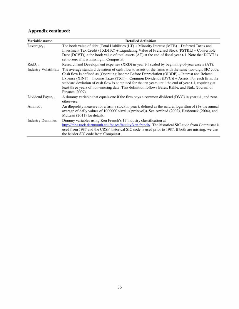
35
Appendix continued:
Variable name Detailed definition
Leveraget-1 The book value of debt (Total Liabilities (LT) + Minority Interest (MTB) – Deferred Taxes and Investment Tax Credit (TXDITC) + Liquidating Value of Preferred Stock (PSTKL) – Convertible Debt (DCVT)) ÷ the book value of total assets (AT) at the end of fiscal year t-1. Note that DCVT is set to zero if it is missing in Compustat.
R&Dt-1 Research and Development expenses (XRD) in year t-1 scaled by beginning-of-year assets (AT).
Industry Volatilityt-1 The average standard deviation of cash flow to assets of the firms with the same two-digit SIC code. Cash flow is defined as (Operating Income Before Depreciation (OIBDP) – Interest and Related Expense (XINT) – Income Taxes (TXT) – Common Dividends (DVC)) ÷ Assets. For each firm, the standard deviation of cash flow is computed for the ten years until the end of year t-1, requiring at least three years of non-missing data. This definition follows Bates, Kahle, and Stulz (Journal of Finance, 2009).
Dividend Payert-1 A dummy variable that equals one if the firm pays a common dividend (DVC) in year t-1, and zero otherwise.
Amihud t An illiquidity measure for a firm’s stock in year t, defined as the natural logarithm of (1+ the annual average of daily values of 1000000 ×ǀretǀ ÷(ǀprcǀ×vol)). See Amihud (2002), Hasbrouck (2004), and McLean (2011) for details.
Industry Dummies Dummy variables using Ken French’s 17 industry classification at http://mba.tuck.dartmouth.edu/pages/faculty/ken.french/. The historical SIC code from Compustat is used from 1987 and the CRSP historical SIC code is used prior to 1987. If both are missing, we use the header SIC code from Compustat.

36
Figure 1. Likelihood of cash depletion sorted by net issue size
In Figure 1A, a firm is defined as running out of cash at the end of fiscal year t if Cash ex post < 0. In Figure 1B, a firm is defined as running out of cash at the end of fiscal year t if Cash ex ante < 0. Net equity issue size and net debt issue size are defined as ∆Equityt÷Assetst-1 and ∆Debtt÷Assetst-1, respectively. See the Appendix for the detailed definitions of ∆Equityt, ∆Debtt, Cash ex post, and Cash ex ante.
17.8%
23.8% 23.0%23.4% 24.9%
29.7%
51.3%
4.6%9.9%
21.1%
32.9%
41.6%
49.2%
74.9%
0%
10%
20%
30%
40%
50%
60%
70%
80%
≤ 0% > 0%, < 1% ≥ 1%, < 2% ≥ 2%, < 3% ≥ 3%, < 4% ≥ 4%, < 5% ≥ 5%
Lik
eli
ho
od
of
Ca
sh D
ep
leti
on
Net Issue Size
Figure 1A: Ex post likelihood of cash depletion at t
sorted by net issue size
Net Equity Issue Net Debt Issue
24.1%
30.8%
25.8% 25.2% 26.7%29.7%
42.4%
22.4%
25.6%
30.2%
35.5% 35.4%37.2%
42.6%
0%
10%
20%
30%
40%
50%
≤ 0% > 0%, < 1% ≥ 1%, < 2% ≥ 2%, < 3% ≥ 3%, < 4% ≥ 4%, < 5% ≥ 5%
Lik
eli
ho
od
of
Ca
sh D
ep
leti
on
Net Issue Size
Figure 1B: Ex ante likelihood of cash depletion at t
sorted by net issue size
Net Equity Issue Net Debt Issue
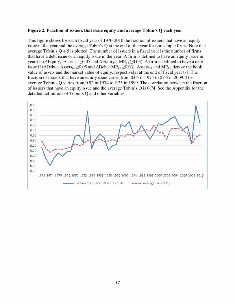
37
Figure 2. Fraction of issuers that issue equity and average Tobin’s Q each year
This figure shows for each fiscal year of 1970-2010 the fraction of issuers that have an equity issue in the year and the average Tobin’s Q at the end of the year for our sample firms. Note that average Tobin’s Q ÷ 5 is plotted. The number of issuers in a fiscal year is the number of firms that have a debt issue or an equity issue in the year. A firm is defined to have an equity issue in year t if (∆Equityt÷Assetst-1 ≥0.05 and ∆Equityt÷ MEt-1 ≥0.03). A firm is defined to have a debt issue if (∆Debtt÷ Assetst-1 ≥0.05 and ∆Debtt÷MEt-1 ≥0.03). Assetst-1 and MEt-1 denote the book value of assets and the market value of equity, respectively, at the end of fiscal year t-1. The fraction of issuers that have an equity issue varies from 0.05 in 1974 to 0.65 in 2009. The average Tobin’s Q varies from 0.92 in 1974 to 2.25 in 1999. The correlation between the fraction of issuers that have an equity issue and the average Tobin’s Q is 0.74. See the Appendix for the detailed definitions of Tobin’s Q and other variables.
0.00
0.05
0.10
0.15
0.20
0.25
0.30
0.35
0.40
0.45
0.50
0.55
0.60
0.65
1972 1974 1976 1978 1980 1982 1984 1986 1988 1990 1992 1994 1996 1998 2000 2002 2004 2006 2008 2010
Fraction of issuers that issue equity Average Tobin's Q ÷ 5

38
Table 1. Sample distribution
This table reports the distribution of firm-year observations in our sample of CRSP- and Compustat-listed firms from 1972-2010. Utility and financial firms are excluded. N denotes the number of firm-year observations. % denotes the number of firm-year observations in a category of security issues as a percent of the total number of firm-year observations in a group. A firm is defined to have a pure equity issue if (∆Equityt÷Assetst-1 ≥0.05 and ∆Equityt÷MEt-1 ≥0.03) and (∆Debtt÷Assetst-1 <0.05 or ∆Debtt÷MEt-1 <0.03). A firm is defined to have a pure debt issue if (∆Equityt÷Assetst-1 <0.05 or ∆Equityt÷MEt-1 <0.03) and (∆Debtt÷Assetst-1 ≥0.05 and ∆Debtt÷MEt-1 ≥0.03). A firm is defined to have dual issues of debt and equity if (∆Equityt÷Assetst-1 ≥0.05 and ∆Equityt÷MEt-1 ≥0.03) and ∆Debtt÷Assetst-1 ≥0.05 and ∆Debtt÷MEt-1 ≥0.03). Assetst-1 and MEt-1 denote the book value of assets and the market value of equity, respectively, at the end of fiscal year t-1. A firm is considered as running out of cash if Cash ex post <0. See the Appendix for the detailed definitions of ∆Equityt, ∆Debtt, and Cash ex post.
N %
All firm-years 116,488 100.0 No security issue 82,297 70.7 Pure debt issue 21,749 18.7 Dual issues of debt and equity 3,110 2.7 Pure equity issue 9,332 8.0 Conditional on external financing 34,191 100.0 Pure debt issue 21,749 63.6 Dual issues of debt and equity 3,110 9.1 Pure equity issue 9,332 27.3 Conditional on external financing and running out of cash 22,954 100.0 Pure debt issue 16,180 70.5 Dual issues of debt and equity 2,753 12.0 Pure equity issue 4,021 17.5 Conditional on external financing and not running out of cash 11,237 100.0 Pure debt issue 5,569 49.6 Dual issues of debt and equity 357.0 3.2 Pure equity issue 5,311 47.3

39
Table 2. Cash flows
This table reports the summary statistics of the cash flow items. In Panels A and B, a firm is defined to have a pure equity issue if (∆Equityt÷Assetst-1 ≥0.05 and ∆Equityt÷MEt-1 ≥0.03) and (∆Debtt÷Assetst-1 <0.05 or ∆Debtt÷MEt-1 <0.03). A firm is defined to have a pure debt issue if (∆Equityt÷Assetst-1 <0.05 or ∆Equityt÷MEt-1 <0.03) and (∆Debtt÷Assetst-1 ≥0.05 and ∆Debtt÷MEt-1 ≥0.03). A firm is defined to have dual issues of debt and equity if (∆Equityt÷Assetst-1 ≥0.05 and ∆Equityt÷MEt-1 ≥0.03) and (∆Debtt÷Assetst-1 ≥0.05 and ∆Debtt÷MEt-1 ≥0.03). Assetst-1 and MEt-1 denote the book value of assets and the market value of equity, respectively, at the end of fiscal year t-1. Panel A reports the means (in percent) of the cash flow items. Panel B reports the means of free cash flows (FCFs) from t-1 to t+2, scaled by Assetst-1, and the likelihoods of the FCFs being negative (in percent). Panels C and D report the means (in percent) for different categories of firms sorted by net equity issue size and net debt issue size, respectively. [1%, 2%) denotes the range of ≥1% and <2%, and other intervals are similarly defined. See the Appendix for the detailed definitions of ∆Equityt, ∆Debtt, and other variables.
Panel A. Mean cash flows (%) for firms sorted by security issues
VARIABLES
No security issue
Pure debt issue
Dual issues
Pure equity issue All
∆Debtt÷Assetst-1 -1.9 18.3 30.4 -4.8 2.5 ∆Equityt÷Assetst-1 -0.4 -0.7 29.3 37.7 3.4 External Financingt ÷Assetst-1 -2.3 17.6 59.7 32.9 5.9 ICFt÷Assetst-1 10.3 10.4 3.7 -0.5 9.3 Investmentst÷Assetst-1 6.7 20.7 41.4 14.6 10.8 Cash Dividendst ÷Assetst-1 1.2 1.0 0.7 0.5 1.1 ∆NWCt÷Assetst-1 0.3 6.3 17.9 17.4 3.3 Financing Deficitt÷Assetst-1 -2.1 17.6 56.3 33 5.9 ∆Non-Cash NWCt ÷Assetst-1 0.4 5.1 6.7 2.5 1.6 ∆Casht÷Assetst-1 -0.0 1.1 10.6 15.1 1.7
Panel B. Free cash flows (%) for firms sorted by security issues
VARIABLES
No security issue
Pure debt issue
Dual issues
Pure equity issue All
FCFt-1÷Assetst-1 -1.3 -5.3 -17.2 -15.7 -3.6 FCFt÷Assetst-1 2.1 -16.7 -46.9 -18.5 -4.3 FCFt+1÷Assetst-1 -1.3 -6.5 -29.8 -22.7 -4.7 FCFt+2÷Assetst-1 -2.1 -5.7 -28.8 -22.1 -5.1 %(FCFt-1<0) 48.9 63.5 79.2 73.8 54.4 %(FCFt<0) 38.2 92.2 97.5 75.8 52.9 %(FCFt+1<0) 46.5 57.4 75.1 73.7 51.5 %(FCFt+2<0) 47.5 51.4 69.6 68.2 50.4

40
Panel C. Means cash flows (%) for firms sorted by ∆Equityt÷Assetst-1
∆equityt÷Assetst-1
VARIABLES ≤0% (0%, 1%) [1%, 2%) [2%, 3%) [3%, 4%) [4%, 5%) ≥5%
∆Debtt÷Assetst-1 1.8 2.4 3.5 3.7 3.7 3.7 4.3 ∆Equityt÷Assetst-1 -1.9 0.3 1.4 2.5 3.5 4.5 33.2 ICFt÷Assetst-1 10.8 9.5 10.7 11.0 11.5 10.4 1.2 Investmentst÷Assetst-1 8.5 9.8 11.9 13.1 12.9 13.0 20.9 Cash Dividendst ÷Assetst-1 1.4 1.1 0.9 0.8 0.7 0.7 0.5 ∆NWCt÷Assetst-1 0.9 1.5 2.9 3.9 5.5 5.1 16.7 ∆Non-Cash NWCt ÷Assetst-1 0.9 1.8 2.5 2.4 2.7 2.2 3.3 ∆Casht÷Assetst-1 0.1 -0.3 0.4 1.6 2.7 3.0 13.4
Panel D. Mean cash flows (%) for firms sorted by ∆Debtt÷Assetst-1
∆Debtt÷Assetst-1
VARIABLES ≤0% (0%, 1%) [1%, 2%) [2%, 3%) [3%, 4%) [4%, 5%) ≥5%
∆Debtt÷Assetst-1 -3.7 0.5 1.5 2.5 3.5 4.5 19.4 ∆Equityt÷Assetst-1 4.0 1.5 1.8 1.3 1.4 1.5 3.4 ICFt÷Assetst-1 9.1 9.7 9.4 9.8 9.5 9.2 9.4 Investmentst÷Assetst-1 6.6 8.6 9.3 10.1 10.6 11.3 23.1 Cash Dividendst ÷Assetst-1 1.1 1.4 1.3 1.3 1.3 1.2 1.0 ∆NWCt÷Assetst-1 1.9 1.8 2.1 2.3 2.6 2.8 7.7 ∆Non-Cash NWCt ÷Assetst-1 0.2 1.4 1.6 2.1 2.5 2.5 5.3 ∆Casht ÷Assetst-1 1.9 0.5 0.5 0.1 0.1 0.4 2.3

41
Table 3. Cash, excess cash, and likelihoods of cash depletion
This table reports the means of cash and excess cash ratios and the likelihoods of cash depletion (in percent). Excess cash ratio subtracts a firm’s cash ratio by the median cash ratio in the same fiscal year for firms in the same tercile of Tobin’s Q and assets that are in the same industry, using the 17 industries classification on Ken French’s web site. See the Appendix and Table 2 for variable definitions.
No security
issue
Pure debt issue
Dual issues
Pure equity issue
All debt issue
All equity issue All
Panel A. Means of cash and excess cash ratios (%) Casht-1÷Assetst-1 15.5 9.0 13.7 23.5 9.6 21.0 14.9 Casht÷Assetst 15.0 7.7 13.8 26.9 8.5 23.6 14.6 Casht+1÷Assetst+1 15.1 7.8 12.6 24.9 8.4 21.9 14.4 Excess (Casht-1÷Assetst-1) 3.7 0.0 0.1 2.5 0.0 1.9 2.8 Excess (Casht÷Assetst) 3.4 -0.7 0.5 5.8 -0.5 4.5 2.8 Excess (Casht+1÷Assetst+1) 3.6 -0.5 0.0 4.4 -0.4 3.3 2.8
Panel B: Hypothetical likelihood of cash depletion (%) (Casht-1+FCFt)<0 6.5 74.4 88.5 43.1 76.2 54.4 24.3 (Casht-1+FCFt-1)<0 22.8 41.0 57.7 40.5 43.1 44.8 28.6 (Casht-1+FCFt+FCFt+1)<0 16.8 70.3 91.4 61.2 72.9 68.7 32.3 (Casht-1+2×FCFt-1)<0 30.5 49.6 68.5 54.7 52.0 58.2 37.0 (Casht-1+FCFt+∆Debtt)<0 2.9 5.1 66.9 56.8 12.8 59.3 9.3 (Casht-1+FCFt+∆Equityt)<0 6.5 78.1 67.3 2.9 76.7 19.0 21.2 [Casht-1+FCFt+0.5×(∆Debtt+∆Equityt)]<0 3.6 56.9 68.9 23.3 58.4 34.7 16.9 (Casht-1+FCFt+∆Debtt+0.5×∆Equityt)<0 1.6 2.9 46.7 33.0 8.4 36.4 5.6 (Casht-1+FCFt+∆Equityt+0.5×∆Debtt)<0 3.6 59.9 50.9 1.7 58.8 14.0 15.2 (Casht-1+FCFt+Cash Dividendst)<0 4.7 70.5 87.8 41.8 72.7 53.3 22.1 (Casht-1+FCFt+FCFt+1+∆Debtt+∆Debtt+1+∆Equityt+1)<0 2.9 4.7 66.2 57.9 12.3 59.9 9.3 (Casht-1+FCFt+∆Debtt–Equity Buybackt)<0 4.1 7.4 67.4 57.4 14.9 59.9 10.7

42
Table 4. Means of control variables sorted by security issues
This table reports the means of the control variables used in the multivariate analysis. A firm is considered as running out of cash if Cash ex post<0. An old firm is defined as one that has been listed on CRSP for more than 10 years. See the Appendix and Table 2 for variable definitions.
Panel A. All firms (N=116,488)
VARIABLES No security
issue Pure debt
issue Dual issues
Pure equity issue
All
Tobin’s Qt-1 1.6 1.6 2.1 2.6 1.7
Returnt-1(%) 17.1 23.0 46.7 44.9 21.2
Returnt+1, t+3(%) 60.3 44.5 10.5 14.9 52.4
Term Spreadt-1(%) 1.1 0.9 1.0 1.2 1.1
Default Spreadt-1(%) 1.1 1.1 1.1 1.1 1.1
Ln(Sales)t-1 6.0 5.9 4.7 4.3 5.8
Ln(Age)t 2.5 2.4 2.0 2.1 2.4
Leveraget-1(%) 44.9 49.4 54.3 47.5 46.2
R&Dt-1 (%) 3.8 2.6 6.2 11.6 4.2
Industry Volatilityt-1 (%) 17.9 15.2 19.3 24.4 17.9
Dividend Payert-1 (%) 47.7 45.8 24.0 17.4 44.3
Panel B. Young firms (N=53,294)
VARIABLES No security
issue Pure debt
issue Dual issues
Pure equity issue
All
Tobin’s Qt-1 1.8 1.6 2.2 2.9 1.9
Returnt-1(%) 17.0 22.9 48.4 46.7 22.6
Returnt+1, t+3(%) 66.2 46.3 6.7 12.8 54.2
Term Spreadt-1(%) 1.0 0.9 0.9 1.2 1.0
Default Spreadt-1(%) 1.1 1.0 1.0 1.1 1.1
Ln(Sales)t-1 5.3 5.3 4.3 3.9 5.1
Ln(Age)t 1.7 1.6 1.6 1.6 1.6
Leveraget-1(%) 43.2 49.8 54.4 45.3 45.1
R&Dt-1 (%) 4.9 3.0 6.8 13.2 5.5
Industry Volatilityt-1 (%) 19.1 15.0 19.4 25.0 19.0
Dividend Payert-1 (%) 31.6 31.6 15.2 10.6 28.7

43
Panel C. Old firms (N=63,194)
VARIABLES No security
issue Pure debt
issue Dual issues
Pure equity issue
All
Tobin’s Qt-1 1.5 1.5 1.8 2.3 1.5
Returnt-1(%) 17.2 23.0 43.6 41.7 20.0
Returnt+1, t+3(%) 56.0 42.9 17.7 18.4 50.9
Term Spreadt-1(%) 1.2 1.0 1.1 1.3 1.1
Default Spreadt-1(%) 1.2 1.1 1.2 1.2 1.1
Ln(Sales)t-1 6.5 6.4 5.5 5.0 6.3
Ln(Age)t 3.1 3.0 2.9 2.9 3.0
Leveraget-1(%) 46.2 49.0 54.1 51.1 47.1
R&Dt-1 (%) 2.9 2.3 5.1 8.9 3.1
Industry Volatilityt-1 (%) 16.9 15.4 19.2 23.5 17.1
Dividend Payert-1 (%) 59.7 58.9 40.6 28.9 57.5
Panel D. Firms that are running out of cash and issuing a security (N=22,954)
VARIABLES Pure debt issue Dual issues Pure equity issue All
Tobin’s Qt-1 1.5 2.1 2.8 1.8
Returnt-1(%) 23.2 46.7 48.7 30.5
Returnt+1, t+3(%) 42.7 8.7 2.8 31.6
Term Spreadt-1(%) 0.9 1.0 1.1 0.9
Default Spreadt-1(%) 1.1 1.1 1.1 1.1
Ln(Sales)t-1 5.8 4.7 4.1 5.4
Ln(Age)t 2.3 2.0 2.0 2.2
Leveraget-1(%) 50.9 55.5 51.1 51.5
R&Dt-1 (%) 2.1 5.2 9.6 3.8
Industry Volatilityt-1 (%) 14.0 18.1 21.0 15.7
Dividend Payert-1 (%) 45.5 25.3 18.3 38.3
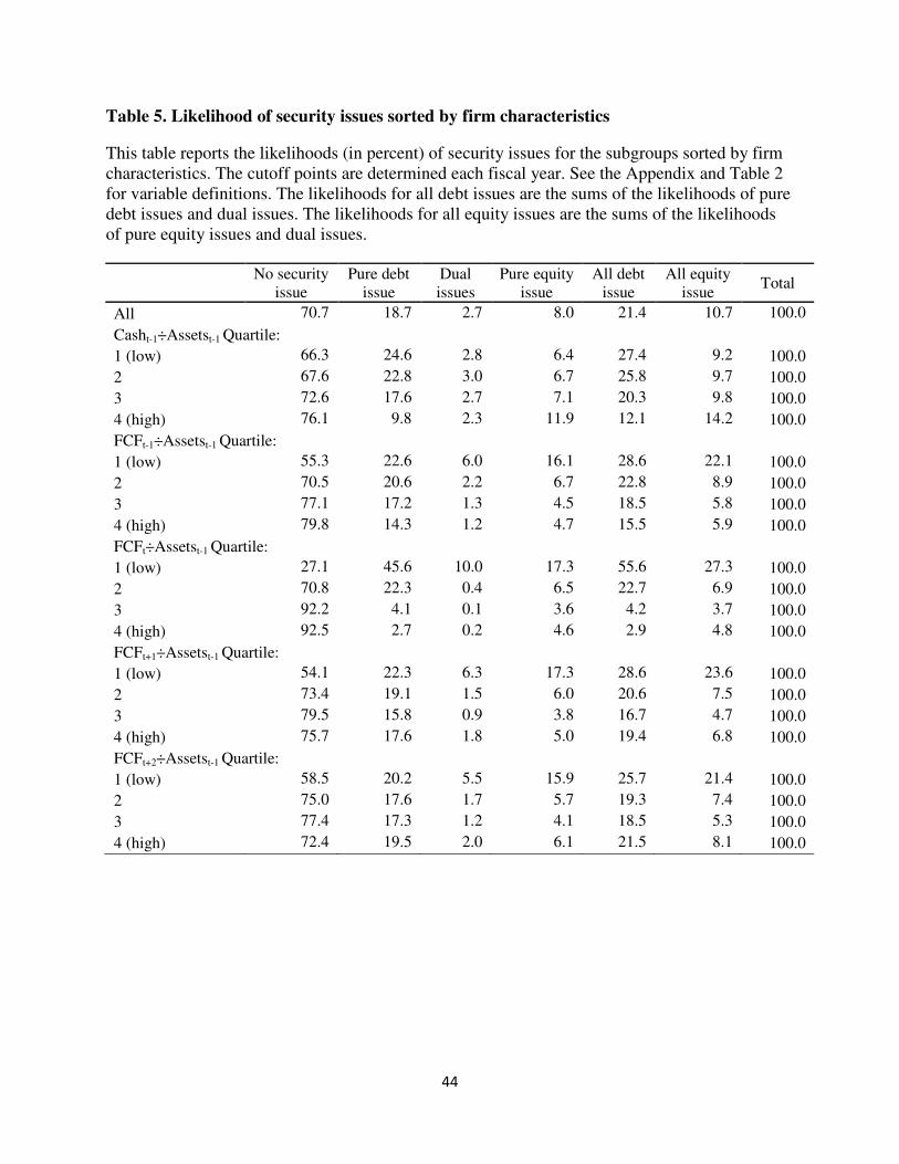
44
Table 5. Likelihood of security issues sorted by firm characteristics
This table reports the likelihoods (in percent) of security issues for the subgroups sorted by firm characteristics. The cutoff points are determined each fiscal year. See the Appendix and Table 2 for variable definitions. The likelihoods for all debt issues are the sums of the likelihoods of pure debt issues and dual issues. The likelihoods for all equity issues are the sums of the likelihoods of pure equity issues and dual issues.
No security
issue Pure debt
issue Dual issues
Pure equity issue
All debt issue
All equity issue
Total
All 70.7 18.7 2.7 8.0 21.4 10.7 100.0
Casht-1÷Assetst-1 Quartile:
1 (low) 66.3 24.6 2.8 6.4 27.4 9.2 100.0
2 67.6 22.8 3.0 6.7 25.8 9.7 100.0
3 72.6 17.6 2.7 7.1 20.3 9.8 100.0
4 (high) 76.1 9.8 2.3 11.9 12.1 14.2 100.0
FCFt-1÷Assetst-1 Quartile:
1 (low) 55.3 22.6 6.0 16.1 28.6 22.1 100.0
2 70.5 20.6 2.2 6.7 22.8 8.9 100.0
3 77.1 17.2 1.3 4.5 18.5 5.8 100.0
4 (high) 79.8 14.3 1.2 4.7 15.5 5.9 100.0
FCFt÷Assetst-1 Quartile:
1 (low) 27.1 45.6 10.0 17.3 55.6 27.3 100.0
2 70.8 22.3 0.4 6.5 22.7 6.9 100.0
3 92.2 4.1 0.1 3.6 4.2 3.7 100.0
4 (high) 92.5 2.7 0.2 4.6 2.9 4.8 100.0
FCFt+1÷Assetst-1 Quartile:
1 (low) 54.1 22.3 6.3 17.3 28.6 23.6 100.0
2 73.4 19.1 1.5 6.0 20.6 7.5 100.0
3 79.5 15.8 0.9 3.8 16.7 4.7 100.0
4 (high) 75.7 17.6 1.8 5.0 19.4 6.8 100.0
FCFt+2÷Assetst-1 Quartile:
1 (low) 58.5 20.2 5.5 15.9 25.7 21.4 100.0
2 75.0 17.6 1.7 5.7 19.3 7.4 100.0
3 77.4 17.3 1.2 4.1 18.5 5.3 100.0
4 (high) 72.4 19.5 2.0 6.1 21.5 8.1 100.0

45
Table 5 Continued:
No security
issue Pure debt
issue Dual issues
Pure equity issue
All debt issue
All equity issue
Total
Cash ex post÷Assetst-1 Quartile:
1 (running out) 22.1 54.4 9.4 14.1 63.8 23.5 100.0
2 82.9 11.1 0.5 5.5 11.6 6.0 100.0
3 88.6 5.6 0.4 5.5 6.0 5.9 100.0
4 89.0 3.6 0.3 7.0 3.9 7.3 100.0
Cash ex ante÷Assetst-1 Quartile:
1 (running out) 56.1 26.3 5.5 12.1 31.8 17.6 100.0
2 70.4 21.4 2.1 6.1 23.5 8.2 100.0
3 75.4 17.0 1.6 6.0 18.6 7.6 100.0
4 80.7 10.0 1.4 7.9 11.4 9.3 100.0
∆Casht÷Assetst-1 Quartile:
1 (low) 75.4 16.7 2.0 5.9 18.7 7.9 100.0
2 73.2 20.8 1.7 4.3 22.5 6.0 100.0
3 71.3 21.4 2.1 5.2 23.5 7.3 100.0
4 (high) 62.7 15.8 4.8 16.7 20.6 21.5 100.0
∆Non-Casht÷Assetst-1 Quartile:
1 (low) 84.9 7.0 1.0 7.2 8.0 8.2 100.0
2 84.7 9.2 0.6 5.5 9.8 6.1 100.0
3 72.5 19.9 1.0 6.7 20.9 7.7 100.0
4 (high) 40.5 38.7 8.1 12.6 46.8 20.7 100.0
Tobin’s Qt-1 Quartile:
1 (low) 79.3 16.4 1.1 3.2 17.5 4.3 100.0
2 72.0 20.4 2.1 5.4 22.5 7.5 100.0
3 67.2 21.4 3.4 8.1 24.8 11.5 100.0
4 (high) 64.1 16.4 4.2 15.3 20.6 19.5 100.0
Stock Returnt-1 Quartile:
1 (low) 72.8 16.2 2.4 8.6 18.6 11.0 100.0
2 73.6 18.6 2.0 5.8 20.6 7.8 100.0
3 72.0 19.5 2.4 6.1 21.9 8.5 100.0
4 (high) 64.2 20.4 4.0 11.5 24.4 15.5 100.0
Stock Returnt+1, t+3 Quartile:
1 (low) 60.0 21.3 4.9 13.8 26.2 18.7 100.0
2 72.1 18.5 2.2 7.2 20.7 9.4 100.0
3 75.5 17.6 1.8 5.2 19.4 7.0 100.0
4 (high) 75.0 17.4 1.8 5.8 19.2 7.6 100.0

46
Table 5 Continued:
No security
issue Pure debt
issue Dual issues
Pure equity issue
All debt issue
All equity issue
Total
Term Spreadt-1 Quartile:
1 (low) 71.3 18.2 2.6 8.0 20.8 10.6 100.0
2 73.6 19.5 1.8 5.1 21.3 6.9 100.0
3 65.5 22.4 3.7 8.4 26.1 12.1 100.0
4 (high) 70.8 17.4 2.7 9.0 20.1 11.7 100.0
Default Spreadt-1 Quartile:
1 (low) 71.3 18.2 2.4 8.0 20.6 10.4 100.0
2 68.5 20.1 3.0 8.4 23.1 11.4 100.0
3 67.6 22.4 3.0 6.9 25.4 9.9 100.0
4 (high) 71.7 17.5 2.6 8.1 20.1 10.7 100.0
Ln(Sales)t-1 Quartile:
1 (low) 63.2 16.0 4.5 16.2 20.5 20.7 100.0
2 70.5 19.4 2.6 7.5 22.0 10.1 100.0
3 72.2 20.5 2.1 5.2 22.6 7.3 100.0
4 (high) 76.6 18.8 1.4 3.2 20.2 4.6 100.0
Aget Quartile:
1 (young) 63.4 19.8 4.3 12.5 24.1 16.8 100.0
2 68.7 18.9 3.1 9.3 22.0 12.4 100.0
3 72.6 18.3 2.1 7.0 20.4 9.1 100.0
4 (old) 77.7 17.7 1.2 3.4 18.9 4.6 100.0
Leveraget-1 Quartile:
1 (low) 77.1 12.4 1.6 8.8 14.0 10.4 100.0
2 70.3 20.2 2.4 7.2 22.6 9.6 100.0
3 68.6 21.6 2.8 7.0 24.4 9.8 100.0
4 (high) 66.6 20.5 3.9 9.0 24.4 12.9 100.0
R&Dt-1 Group:
0 (zero or missing) 68.8 21.9 3.1 6.2 25.0 9.3 100.0
1 (low) 75.7 17.5 1.6 5.2 19.1 6.8 100.0
2 (high) 69.4 13.1 2.8 14.7 15.9 17.5 100.0
Industry Volatilityt-1 Quartile:
1 (low) 73.2 20.6 1.9 4.3 22.5 6.2 100.0
2 70.8 19.5 2.7 7.0 22.2 9.7 100.0
3 69.7 17.4 3.0 9.8 20.4 12.8 100.0
4 (high) 68.4 16.7 3.2 11.8 19.9 15.0 100.0
Dividend Payert-1:
0 (Non-payer) 66.3 18.2 3.6 11.9 21.8 15.5 100.0
1 (Payer) 76.1 19.3 1.4 3.1 20.7 4.5 100.0

47
Table 6. Multinomial logit for the issuance and choice of securities
This table reports the results for the multinomial logit regressions for the decision to issue only debt, only equity, both debt and equity, or neither debt nor equity. A firm is defined to have a pure equity issue if (∆Equityt÷Assetst-1 ≥0.05 and ∆Equityt÷MEt-1 ≥0.03) and (∆Debtt÷Assetst-1
<0.05 or ∆Debtt÷MEt-1 <0.03). A firm is defined to have a pure debt issue if (∆Equityt÷Assetst-1
<0.05 or ∆Equityt÷MEt-1 <0.03) and (∆Debtt÷Assetst-1 ≥0.05 and ∆Debtt÷MEt-1 ≥0.03). A firm is defined to have dual issues of debt and equity if (∆Equityt÷Assetst-1 ≥0.05 and ∆Equityt÷MEt-1
≥0.03) and (∆Debtt÷Assetst-1 ≥0.05 and ∆Debtt÷MEt-1 ≥0.03). Assetst-1 and MEt-1 denote the book value of assets and the market value of equity, respectively, at the end of fiscal year t-1. Returns are measured as decimals (e.g., a 20% return is measured as 0.20) and spreads are measured as annual percentages. Panel A reports the coefficients and z-statistics, with the base category consisting of firm-years with no security issues. Panel B reports the economic effects. To compute the economic effect of an independent variable on a pure equity issue, for example, we first add one standard deviation of the variable’s sample values to its actual value for each observation in our sample, without changing the actual values of other independent variables, and compute the predicted average likelihood of a pure equity issue for all observations using the regressions coefficients. We also subtract its actual value by one standard deviation, without changing the actual values of other variables, and compute the predicted average likelihood of a pure equity issue. We then compute the change in the predicted average likelihood as the economic effect of this variable on a pure equity issue. In the last two columns of Panel B, the subtotal economic effects are reported. For example, the subtotal economic effect of Casht-1
÷Assetst-1 on all debt issues is the sum of the economic effects of Casht-1÷Assetst-1 on pure debt issues and dual issues of debt and equity. See the Appendix and Table 2 for variable definitions. Z-statistics are in parentheses, calculated using robust standard errors corrected for heteroskedasticity and clustering at the company level. ***, **, and * indicates significance at the 1%, 5%, and 10% level.
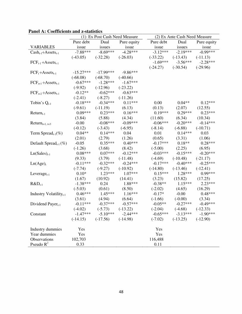
48
Panel A: Coefficients and z-statistics (1) Ex Post Cash Need Measure (2) Ex Ante Cash Need Measure
VARIABLES Pure debt
issue Dual issues
Pure equity issue
Pure debt
issue Dual issues
Pure equity issue
Casht-1÷Assetst-1 -7.88*** -8.69*** -4.28*** -3.12*** -2.19*** -0.99*** (-43.05) (-32.28) (-26.03) (-33.22) (-13.43) (-11.13)
FCFt-1 ÷Assetst-1 -1.69*** -3.56*** -2.28*** (-24.27) (-30.54) (-29.96) FCFt ÷Assetst-1 -15.27*** -17.99*** -9.86*** (-68.08) (-68.70) (-40.66) FCFt+1 ÷Assetst-1 -0.67*** -1.28*** -1.67*** (-9.92) (-12.96) (-23.22) FCFt+2 ÷Assetst-1 -0.12** -0.62*** -0.63*** (-2.41) (-8.27) (-11.26) Tobin’s Qt-1 -0.18*** -0.34*** 0.11*** 0.00 0.04** 0.12***
(-9.61) (-11.19) (6.13) (0.13) (2.07) (12.55)
Returnt-1 0.09*** 0.23*** 0.16*** 0.19*** 0.29*** 0.23***
(3.84) (5.88) (4.34) (11.60) (6.34) (10.34)
Returnt+1, t+3 -0.00 -0.08*** -0.09*** -0.06*** -0.20*** -0.14***
(-0.12) (-3.43) (-6.95) (-8.14) (-6.88) (-10.71)
Term Spreadt-1(%) 0.04** 0.14*** 0.04 0.01 0.14*** 0.03
(2.01) (2.79) (1.26) (0.65) (3.31) (1.06)
Default Spreadt-1 (%) -0.05 0.35*** 0.40*** -0.17*** 0.18** 0.28***
(-1.26) (3.68) (8.42) (-5.00) (2.25) (6.95)
Ln(Sales)t-1 0.08*** 0.07*** -0.12*** -0.03*** -0.15*** -0.20***
(9.33) (3.79) (-11.48) (-4.69) (-10.48) (-21.17)
Ln(Age)t -0.11*** -0.32*** -0.24*** -0.17*** -0.40*** -0.25***
(-7.74) (-9.27) (-10.92) (-14.80) (-13.46) (-12.41)
Leveraget-1 0.10* 1.23*** 1.07*** 0.15*** 1.28*** 0.99***
(1.67) (10.92) (14.41) (3.23) (15.82) (17.25)
R&Dt-1 -1.38*** 0.24 1.88*** -0.38** 1.15*** 2.23***
(-5.03) (0.61) (8.50) (-2.02) (4.65) (16.29)
Industry Volatilityt-1 0.46*** 1.45*** 1.16*** -0.17* -0.00 0.48***
(3.61) (4.94) (6.64) (-1.66) (-0.00) (3.34)
Dividend Payert-1 -0.11*** -0.37*** -0.57*** -0.05** -0.27*** -0.49***
(-4.02) (-5.73) (-13.22) (-2.04) (-4.68) (-12.33)
Constant -1.47*** -5.10*** -2.44*** -0.65*** -3.13*** -1.90*** (-14.15) (-17.56) (-14.98) (-7.02) (-13.25) (-12.90)
Industry dummies Yes Yes Year dummies Yes Yes Observations 102,703 116,488 Pseudo R2 0.33 0.11

49
Panel B. Economic effects (%)
VARIABLES No security
issue Pure debt
issue Dual issues
Pure equity issue
All debt issues
All equity issues
Regression (1): Casht-1÷Assetst-1 30.4 -25.4 -2.5 -2.5 -27.9 -5.0 FCFt ÷Assetst-1 60.1 -47.4 -6.2 -6.5 -53.6 -12.7 FCFt+1 ÷Assetst-1 5.8 -1.5 -0.6 -3.7 -2.1 -4.3 FCFt+2 ÷Assetst-1 2.0 0.2 -0.5 -1.7 -0.3 -2.2 Tobin’s Qt-1 3.5 -4.9 -1.4 2.8 -6.3 1.4 Returnt-1 -3.0 1.0 0.6 1.4 1.6 2.0 Returnt+1, t+3 1.6 1.0 -0.5 -2.1 0.5 -2.6 Term Spreadt-1 (%) -1.4 0.5 0.5 0.3 1.0 0.8 Default Spreadt-1 (%) -1.3 -1.7 0.6 2.3 -1.1 2.9 Ln(Sales)t-1 -0.9 4.0 0.4 -3.5 4.4 -3.1 Ln(Age)t 3.3 -0.7 -0.7 -1.8 -1.4 -2.5 Leveraget-1 -2.4 -1.0 0.9 2.5 -0.1 3.4 R&Dt-1 0.8 -3.4 0.2 2.3 -3.2 2.5 Industry Volatilityt-1 -2.7 0.5 0.6 1.6 1.1 2.2 Dividend Payert-1 3.1 0.1 -0.4 -2.8 -0.3 -3.2 Regression (2): Casht-1÷Assetst-1 17.1 -15.6 -1.1 -0.4 -16.7 -1.5 FCFt-1 ÷Assetst-1 11.7 -6.1 -2.2 -3.4 -8.3 -5.6 Tobin’s Qt-1 -1.7 -0.5 0.1 2.1 -0.4 2.2 Returnt-1 -7.8 4.6 1.0 2.2 5.6 3.2 Returnt+1, t+3 6.9 -2.3 -1.6 -3.1 -3.9 -4.7 Term Spreadt-1 (%) -1.2 0.1 0.8 0.3 0.9 1.1 Default Spreadt-1 (%) 0.6 -3.0 0.4 2.0 -2.6 2.4 Ln(Sales)t-1 6.2 -0.3 -1.1 -4.8 -1.4 -5.9 Ln(Age)t 6.5 -3.3 -1.3 -1.9 -4.6 -3.2 Leveraget-1 -3.9 0.1 1.2 2.6 1.3 3.8 R&Dt-1 -1.3 -1.7 0.4 2.6 -1.3 3.0 Industry Volatilityt-1 0.0 -1.0 0.0 1.0 -1.0 1.0 Dividend Payert-1 3.1 0.1 -0.4 -2.7 -0.3 -3.1

50
Table 7. Cash needs, cash changes, and cash sources This table reports the results for the firm fixed effects regressions for cash changes. In Panel A, the dependent variable is ∆Casht×100÷Assetst-1. The explanatory variables measure firm fundamentals. The dependent variable in Panel B is Res ∆Casht×100÷Assetst-1, or the residuals from the regressions in Panel A. The explanatory variables measure market conditions. In regressions (1), (5), and (9) of Panel C, the dependent variable is ∆Casht÷Assetst-1. In regressions (2), (6), and (10) of Panel C, the dependent variable is Fitted ∆Casht×100 ÷Assetst-1, or the fitted values from the regressions in Panel A (the ∆Casht due to fundamentals). In regressions (3), (7), and (11), the dependent variable is Fitted Res ∆Casht×100÷Assetst-1, or the fitted values from the regressions in Panel B (the ∆Casht due to market conditions). In regressions (4), (8), and (12), the dependent variable is Res Res ∆Casht×100÷Assetst-1, or the residuals from the regressions in Panel B (the unexplained ∆Casht). A firm is defined to have an equity issue in year t if (∆Equityt÷Assetst-1 ≥0.05 and ∆Equityt÷MEt-1 ≥0.03). A firm is defined to have a debt issue in year t if (∆Debtt÷Assetst-1 ≥0.05 and ∆Debtt÷MEt-1 ≥0.03). Assetst-1 and MEt-1 denote the book value of assets and the market value of equity, respectively, at the end of fiscal year t-1. Returns are measured as decimals (e.g., a 20% return is measured as 0.20) and spreads are measured as annual percentages. See the Appendix and Table 2 for variable definitions. N denotes the number of observations. Adjusted within R2s for the firm fixed effects regressions are reported. T-statistics are in parentheses, calculated using robust standard errors corrected for heteroskedasticity and clustering at the company level. ***, **, and * indicates significance at the 1%, 5%, and 10% level.
Panel A: Dependent variable is ∆Casht×100÷Assetst-1 Variables (1) Full Sample (2) Equity Issue Sample (3) Debt Issue Sample
Casht-1÷Assetst-1 -44.3*** -42.3*** -52.6*** (-43.2) (-10.4) (-20.3) ∆Non-Cash Assetst÷Assetst-1 2.1*** 5.2*** 1.9*** (6.7) (5.5) (4.5) FCFt+1 ÷Assetst-1 -13.2*** -18.4*** -9.5*** (-25.9) (-13.8) (-11.8) FCFt+2 ÷Assetst-1 -5.5*** -7.6*** -3.1*** (-14.8) (-7.7) (-5.2) Ln(Assets)t-1 -5.5*** -7.9*** -2.9*** (-21.2) (-7.8) (-5.5) Ln(Sales)t-1 3.0*** 4.4*** 1.7*** (11.7) (5.6) (3.4) Ln(Age)t 0.2 0.3 0.5 (1.5) (0.2) (1.5) Leveraget-1 -0.4 -4.6** 0.7 (-0.8) (-2.0) (0.7) R&Dt-1 27.9*** 29.3*** 21.7*** (10.7) (5.1) (3.0) Industry Volatilityt-1 1.5 -7.1 3.5* (1.6) (-1.0) (1.9) Dividend Payert-1 -0.3 -0.6 0.0 (-1.6) (-0.4) (0.0) Constant 21.9*** 36.4*** 11.1*** (22.7) (7.1) (6.2) Year Dummies Yes Yes Yes N 102,703 10,785 21,825 Adjusted Within R2 0.18 0.20 0.17

51
Panel B: Dependent variable is Res ∆Casht×100 ÷Assetst-1, the residuals from the Panel A
regressions Variables (1) Full Sample (2) Equity Issue Sample (3) Debt Issue Sample
Tobin’s Qt-1 2.3*** 4.2*** 2.2*** (19.3) (10.3) (6.9) Returnt-1 0.3*** 0.2 0.3 (4.6) (0.6) (1.4) Returnt+1, t+3 -0.2** -1.7*** -0.3*** (-2.5) (-7.7) (-3.2) Term Spreadt-1 (%) 0.1 0.4 0.0 (1.4) (1.4) (0.3) Default Spreadt-1 (%) 0.9*** 2.0*** 0.6** (9.9) (3.2) (2.4) Constant -4.9*** -13.0*** -4.2*** (-19.3) (-10.3) (-6.8) N 102,703 10,785 21,825 Adjusted Within R2 0.03 0.07 0.02
Panel C: Sources of the cash change Dependent
∆Equityt
÷Assetst-1
∆Debtt
÷Assetst-1
ICFt
÷Assetst-1 Constant
Within
variable Coeff. t-Stat Coeff. t-Stat Coeff. t-Stat Coeff. t-Stat N Adj. R2
Full Sample
(1) ∆Casht×100÷Assetst-1 59.8*** 73.7 10.8*** 14.1 26.8*** 32.4 -3.0*** -33.0 102,703 0.40
(2) Fitted ∆Casht 13.6*** 50.0 4.8*** 19.4 5.6*** 14.0 0.7*** 18.4 102,703 0.12
(3) Fitted Res ∆Casht 4.2*** 33.3 1.9*** 19.7 4.3*** 21.5 -0.6*** -32.4 102,703 0.11
(4) Unexplained ∆Casht 42.0*** 52.4 4.0*** 5.7 16.9*** 19.0 -3.2*** -32.3 102,703 0.24
Equity Issue Sample
(5) ∆Casht×100÷Assetst-1 65.4*** 48.7 10.1*** 5.0 32.2*** 15.7 -9.6*** -19.0 10,785 0.54
(6) Fitted ∆Casht 17.9*** 28.1 9.4*** 10.3 6.4*** 5.2 7.9*** 34.2 10,785 0.22
(7) Fitted Res ∆Casht 9.2*** 23.0 2.5*** 5.4 0.8 1.1 -3.4*** -23.6 10,785 0.18
(8) Unexplained ∆Casht 38.3*** 27.2 -1.8 -0.9 25.1*** 10.7 -14.1*** -27.0 10,785 0.26
Debt Issue Sample
(9) ∆Casht×100÷Assetst-1 29.6*** 13.8 14.1*** 12.1 12.5*** 6.4 -2.4*** -8.5 21,825 0.16
(10) Fitted ∆Casht 8.8*** 13.8 0.7** 2.0 5.8*** 8.1 1.5*** 15.0 21,825 0.06
(11) Fitted Res ∆Casht 1.9*** 7.7 2.3*** 16.3 1.8*** 6.3 -0.7*** -18.8 21,825 0.11
(12) Unexplained ∆Casht 18.8*** 9.6 11.0*** 9.9 4.8** 2.5 -3.2*** -11.7 21,825 0.09

52
Table 8: Mulitinomial logit for the debt-equity choice, conditional on issuing a security
This table reports the results for the multinomial logit regressions for the decision to issue only debt, only equity, or both debt and equity, conditional on issuing a security. A firm is defined to have a pure equity issue if (∆Equityt÷Assetst-1 ≥0.05 and ∆Equityt÷MEt-1 ≥0.03) and (∆Debtt÷Assetst-1 <0.05 or ∆Debtt÷MEt-1 <0.03). A firm is defined to have a pure debt issue if (∆Equityt÷Assetst-1 <0.05 or ∆Equityt÷MEt-1 <0.03) and (∆Debtt÷Assetst-1 ≥0.05 and ∆Debtt÷MEt-1 ≥0.03). A firm is defined to have dual issues of debt and equity if (∆Equityt÷Assetst-1 ≥0.05 and ∆Equityt÷MEt-1 ≥0.03) and (∆Debtt÷Assetst-1 ≥0.05 and ∆Debtt÷MEt-1 ≥0.03). Assetst-1 and MEt-1 denote the book value of assets and the market value of equity, respectively, at the end of fiscal year t-1. Returns are measured as decimals (e.g., a 20% return is measured as 0.20) and spreads are measured as annual percentages. Panel A reports the coefficients and z-statistics, with the base category consisting of firm-years with pure debt issues. Panel B reports the economic effects. To compute the economic effect of an independent variable on a pure equity issue, for example, we first add one standard deviation of the variable’s sample values to its actual value for each observation in our sample, without changing the actual values of other independent variables, and compute the predicted average likelihood of a pure equity issue for all observations using the regressions coefficients. We also subtract its actual value by one standard deviation, without changing the actual values of other variables, and compute the predicted average likelihood of a pure equity issue. We then compute the change in the predicted average likelihood as the economic effect of this variable on a pure equity issue. In the last two columns of Panel B, the subtotal economic effects are reported. For example, the subtotal economic effect of Casht-1÷Assetst-1 on all debt issues is the sum of the economic effects of Casht-1 ÷Assetst-1 on pure debt issues and dual issues of debt and equity. See the Appendix and Table 2 for variable definitions. Z-statistics are in parentheses, calculated using robust standard errors corrected for heteroskedasticity and clustering at the company level. ***, **, and * indicates significance at the 1%, 5%, and 10% level.

53
Panel A: Coefficients and z-statistics (1) Ex Post Cash Need Measure (2) Ex Ante Cash Need Measure
VARIABLES Dual issues Pure equity issue Dual issues Pure equity issue
Casht-1÷Assetst-1 -0.65*** 2.21*** 0.83*** 1.94*** (-3.14) (15.98) (4.84) (15.81)
FCFt-1 ÷Assetst-1 -2.06*** -0.73*** (-16.84) (-7.73) FCFt ÷Assetst-1 -2.87*** 2.82*** (-28.40) (24.31) FCFt+1 ÷Assetst-1 -0.63*** -0.72*** (-8.16) (-12.19) FCFt+2 ÷Assetst-1 -0.51*** -0.41*** (-8.08) (-8.22) Tobin’s Qt-1 -0.12*** 0.27*** 0.06*** 0.18***
(-4.48) (14.17) (2.91) (11.16)
Returnt-1 0.19*** 0.13*** 0.26*** 0.16***
(7.66) (6.62) (10.80) (8.23)
Returnt+1, t+3 -0.08*** -0.08*** -0.10*** -0.06***
(-3.47) (-5.77) (-4.45) (-5.23)
Term Spreadt-1 (%) 0.10* -0.00 0.12*** 0.01
(1.92) (-0.08) (2.66) (0.40)
Default Spreadt-1 (%) 0.43*** 0.48*** 0.38*** 0.50***
(4.57) (8.41) (4.56) (9.37)
Ln(Sales)t-1 -0.03 -0.24*** -0.12*** -0.17***
(-1.59) (-18.62) (-8.22) (-15.29)
Ln(Age)t -0.21*** -0.12*** -0.22*** -0.09***
(-6.11) (-4.97) (-7.19) (-3.97)
Leveraget-1 1.23*** 0.93*** 1.24*** 0.85***
(11.46) (10.97) (13.82) (11.06)
R&Dt-1 1.93*** 2.97*** 1.46*** 2.40***
(5.75) (11.45) (5.12) (10.51)
Industry Volatilityt-1 1.03*** 0.59*** 0.41 0.90***
(3.55) (2.96) (1.64) (5.03)
Dividend Payert-1 -0.25*** -0.32*** -0.21*** -0.39***
(-3.87) (-7.04) (-3.67) (-9.48)
Constant -3.78*** -0.96*** -2.77*** -1.56*** (-12.98) (-5.13) (-11.17) (-8.80)
Industry dummies Yes Yes Year dummies Yes Yes Observations 29,955 34,191 Pseudo R2 0.24 0.17

54
Panel B. Economic effects (%)
VARIABLES Pure debt
issue Dual issues
Pure equity issue
All debt issues
All equity issues
Regression (1): Casht-1÷Assetst-1 -8.7 -3.2 11.9 -11.9 8.7 FCFt ÷Assetst-1 -10.0 -12.8 22.8 -22.8 10.0 FCFt+1 ÷Assetst-1 7.7 -1.8 -5.9 5.9 -7.7 FCFt+2 ÷Assetst-1 5.7 -2.0 -3.7 3.7 -5.7 Tobin’s Qt-1 -7.9 -3.8 11.7 -11.7 7.9 Returnt-1 -4.9 1.9 3.0 -3.0 4.9 Returnt+1, t+3 4.3 -1.2 -3.2 3.1 -4.4 Term Spreadt-1 (%) -1.0 1.5 -0.5 0.5 1.0 Default Spreadt-1 (%) -7.8 1.9 5.9 -5.9 7.8 Ln(Sales)t-1 12.4 1.1 -13.6 13.5 -12.5 Ln(Age)t 4.1 -1.9 -2.2 2.2 -4.1 Leveraget-1 -7.9 3.0 5.0 -4.9 8.0 R&Dt-1 -10.5 1.6 8.9 -8.9 10.5 Industry Volatilityt-1 -3.6 1.7 1.9 -1.9 3.6 Dividend Payert-1 5.0 -1.0 -4.0 4.0 -5.0 Regression (2): Casht-1÷Assetst-1 -10.4 0.3 10.1 -10.1 10.4 FCFt-1 ÷Assetst-1 7.5 -5.5 -2.0 2.0 -7.5 Tobin’s Qt-1 -7.5 -0.2 7.8 -7.7 7.6 Returnt-1 -6.7 3.1 3.6 -3.6 6.7 Returnt+1, t+3 4.0 -1.9 -2.1 2.1 -4.0 Term Spreadt-1 (%) -1.7 2.1 -0.3 0.4 1.8 Default Spreadt-1 (%) -8.1 1.5 6.6 -6.6 8.1 Ln(Sales)t-1 11.5 -1.9 -9.6 9.6 -11.5 Ln(Age)t 3.6 -2.4 -1.2 1.2 -3.6 Leveraget-1 -7.9 3.4 4.5 -4.5 7.9 R&Dt-1 -8.8 1.0 7.8 -7.8 8.8 Industry Volatilityt-1 -4.0 0.2 3.8 -3.8 4.0 Dividend Payert-1 6.0 -0.6 -5.4 5.4 -6.0

55
Table 9: Mulitinomial logit for the debt-equity choice, conditional on running out of cash
and issuing a security
This table reports the results for the multinomial logit regressions for the decision to issue only debt, only equity, or both debt and equity, conditional on running out of cash and issuing a security. A firm is defined to have a pure equity issue if (∆Equityt÷Assetst-1 ≥0.05 and ∆Equityt÷MEt-1 ≥0.03) and (∆Debtt÷Assetst-1 <0.05 or ∆Debtt÷MEt-1 <0.03). A firm is defined to have a pure debt issue if (∆Equityt÷Assetst-1 <0.05 or ∆Equityt÷MEt-1 <0.03) and (∆Debtt÷Assetst-1 ≥0.05 and ∆Debtt÷MEt-1 ≥0.03). A firm is defined to have dual issues of debt and equity if (∆Equityt÷Assetst-1 ≥0.05 and ∆Equityt÷MEt-1 ≥0.03) and (∆Debtt÷Assetst-1 ≥0.05 and ∆Debtt÷MEt-1 ≥0.03). Assetst-1 and MEt-1 denote the book value of assets and the market value of equity, respectively, at the end of fiscal year t-1. Returns are measured as decimals (e.g., a 20% return is measured as 0.20) and spreads are measured as annual percentages. The sample used for regression (1) requires Cash ex post<0, and the sample used for regression (2) requires Cash ex ante<0. Panel A reports the coefficients and z-statistics, with the base category consisting of firm-years with pure debt issues. Panel B reports the economic effects. To compute the economic effect of an independent variable on a pure equity issue, for example, we first add one standard deviation of the variable’s sample values to its actual value for each observation in our sample, without changing the actual values of other independent variables, and compute the predicted average likelihood of a pure equity issue for all observations using the regressions coefficients. We also subtract its actual value by one standard deviation, without changing the actual values of other variables, and compute the predicted average likelihood of a pure equity issue. We then compute the change in the predicted average likelihood as the economic effect of this variable on a pure equity issue. In the last two columns of Panel B, the subtotal economic effects are reported. For example, the subtotal economic effect of Casht-1÷Assetst-1 on all debt issues is the sum of the economic effects of Casht-1÷Assetst-1 on pure debt issues and dual issues of debt and equity. See the Appendix and Table 2 for variable definitions. Z-statistics are in parentheses, calculated using robust standard errors corrected for heteroskedasticity and clustering at the company level. ***, **, and * indicates significance at the 1%, 5%, and 10% level.
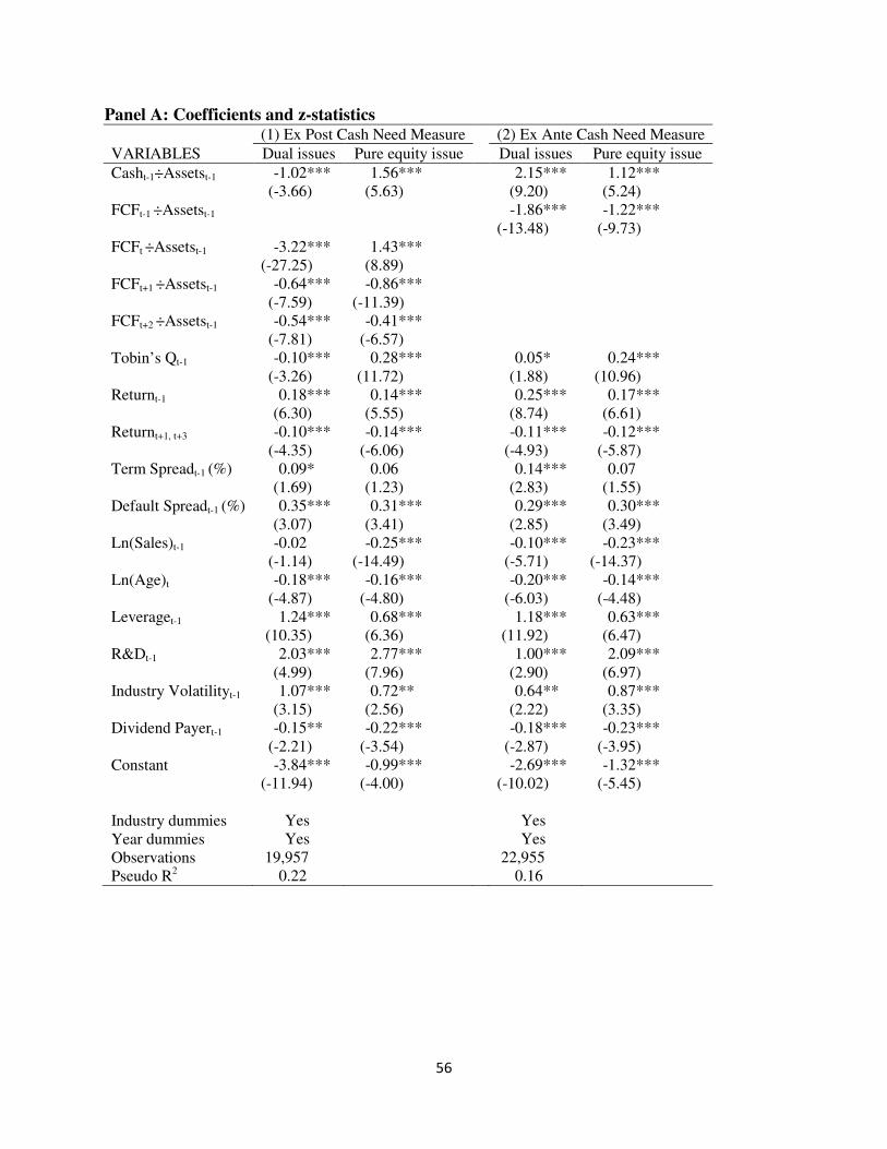
56
Panel A: Coefficients and z-statistics (1) Ex Post Cash Need Measure (2) Ex Ante Cash Need Measure
VARIABLES Dual issues Pure equity issue Dual issues Pure equity issue
Casht-1÷Assetst-1 -1.02*** 1.56*** 2.15*** 1.12*** (-3.66) (5.63) (9.20) (5.24)
FCFt-1 ÷Assetst-1 -1.86*** -1.22*** (-13.48) (-9.73) FCFt ÷Assetst-1 -3.22*** 1.43*** (-27.25) (8.89) FCFt+1 ÷Assetst-1 -0.64*** -0.86*** (-7.59) (-11.39) FCFt+2 ÷Assetst-1 -0.54*** -0.41*** (-7.81) (-6.57) Tobin’s Qt-1 -0.10*** 0.28*** 0.05* 0.24***
(-3.26) (11.72) (1.88) (10.96)
Returnt-1 0.18*** 0.14*** 0.25*** 0.17***
(6.30) (5.55) (8.74) (6.61)
Returnt+1, t+3 -0.10*** -0.14*** -0.11*** -0.12***
(-4.35) (-6.06) (-4.93) (-5.87)
Term Spreadt-1 (%) 0.09* 0.06 0.14*** 0.07
(1.69) (1.23) (2.83) (1.55)
Default Spreadt-1 (%) 0.35*** 0.31*** 0.29*** 0.30***
(3.07) (3.41) (2.85) (3.49)
Ln(Sales)t-1 -0.02 -0.25*** -0.10*** -0.23***
(-1.14) (-14.49) (-5.71) (-14.37)
Ln(Age)t -0.18*** -0.16*** -0.20*** -0.14***
(-4.87) (-4.80) (-6.03) (-4.48)
Leveraget-1 1.24*** 0.68*** 1.18*** 0.63***
(10.35) (6.36) (11.92) (6.47)
R&Dt-1 2.03*** 2.77*** 1.00*** 2.09***
(4.99) (7.96) (2.90) (6.97)
Industry Volatilityt-1 1.07*** 0.72** 0.64** 0.87***
(3.15) (2.56) (2.22) (3.35)
Dividend Payert-1 -0.15** -0.22*** -0.18*** -0.23***
(-2.21) (-3.54) (-2.87) (-3.95)
Constant -3.84*** -0.99*** -2.69*** -1.32*** (-11.94) (-4.00) (-10.02) (-5.45)
Industry dummies Yes Yes Year dummies Yes Yes Observations 19,957 22,955 Pseudo R2 0.22 0.16

57
Panel B. Economic effects (%)
VARIABLES Pure debt
issue Dual issues
Pure equity issue
All debt issues
All equity issues
Regression (1): Casht-1÷Assetst-1 -1.9 -2.9 4.8 -4.8 1.9 FCFt ÷Assetst-1 4.3 -16.0 11.8 -11.7 -4.2 FCFt+1 ÷Assetst-1 8.0 -2.4 -5.6 5.6 -8.0 FCFt+2 ÷Assetst-1 5.6 -2.9 -2.7 2.7 -5.6 Tobin’s Qt-1 -5.5 -4.0 9.5 -9.5 5.5 Returnt-1 -4.4 2.2 2.1 -2.2 4.3 Returnt+1, t+3 5.9 -1.8 -4.1 4.1 -5.9 Term Spreadt-1 (%) -2.6 1.5 1.1 -1.1 2.6 Default Spreadt-1 (%) -4.7 2.2 2.5 -2.5 4.7 Ln(Sales)t-1 9.5 1.4 -10.9 10.9 -9.5 Ln(Age)t 4.4 -2.0 -2.4 2.4 -4.4 Leveraget-1 -6.2 4.0 2.2 -2.2 6.2 R&Dt-1 -7.3 2.1 5.1 -5.2 7.2 Industry Volatilityt-1 -3.5 2.0 1.5 -1.5 3.5 Dividend Payert-1 2.9 -0.8 -2.1 2.1 -2.9 Regression (2): Casht-1÷Assetst-1 -6.3 4.5 1.8 -1.8 6.3 FCFt-1 ÷Assetst-1 9.3 -5.8 -3.5 3.5 -9.3 Tobin’s Qt-1 -7.0 -0.6 7.6 -7.6 7.0 Returnt-1 -6.4 3.8 2.6 -2.6 6.4 Returnt+1, t+3 5.5 -2.2 -3.3 3.3 -5.5 Term Spreadt-1 (%) -3.6 2.6 1.0 -1.0 3.6 Default Spreadt-1 (%) -4.4 1.9 2.6 -2.5 4.5 Ln(Sales)t-1 10.9 -1.3 -9.6 9.6 -10.9 Ln(Age)t 4.4 -2.6 -1.8 1.8 -4.4 Leveraget-1 -6.4 4.5 1.8 -1.9 6.3 R&Dt-1 -5.1 0.8 4.3 -4.3 5.1 Industry Volatilityt-1 -3.3 1.0 2.2 -2.3 3.2 Dividend Payert-1 3.3 -1.1 -2.1 2.2 -3.2

58
Table 10. Time-varying liquidity, precautionary savings, and net equity issue size
The dependent variable is ∆Equityt×100÷Assetst-1, where ∆Equityt is the net equity issue in fiscal
year t. A firm is defined to have an equity issue if (∆Equityt÷Assetst-1 ≥0.05 and ∆Equityt÷MEt-1
≥0.03). Assetst-1 and MEt-1 denote the book value of assets and the market value of equity,
respectively, at the end of fiscal year t-1. Returns are measured as decimals (e.g., a 20% return is
measured as 0.20) and spreads are measured as annual percentages. The regressions include firm
fixed effects and year fixed effects. Amihudt is an illiquidity measure, computed for the calendar
year that ends prior to the end of fiscal year t. This measure is obtained from Joel Hasbrouck’s
website that contains the 1926-2005 liquidity estimates. Thus, the sample for this table excludes
almost all observations for which this measure has a missing value after 2005. See the Appendix
and Table 2 for other variable definitions. T-statistics are in parentheses, calculated using robust
standard errors corrected for heteroskedasticity and clustering at the company level. ***, **, and
* indicates significance at the 1%, 5%, and 10% level.

59
Table 10 Continued: Full Sample Equity Issue Sample
VARIABLES (1) (2) (3) (4)
R&Dt-1 27.83*** 19.52*** 23.70*** 8.67 (9.23) (6.85) (3.54) (1.36) Industry Volatilityt-1 -3.90*** -4.27*** -10.92 -5.83 (-3.77) (-4.27) (-1.32) (-0.70) Dividend Payert-1 -0.93*** -0.64*** -1.52 -2.14 (-4.19) (-3.04) (-0.94) (-1.35) Amihudt -0.76*** -0.07 (-5.25) (-0.05) R&Dt-1× Amihudt -13.54*** -11.52 (-6.12) (-1.54) Industry Volatility× Amihudt -0.03 -8.88 (-0.05) (-1.59) Dividend Payert-1× Amihudt 0.55*** 1.57 (4.19) (0.89) Amihudt-1 -0.75*** 1.33 (-4.95) (1.17) R&Dt-1× Amihudt-1 12.32*** 24.50*** (3.46) (4.10) Industry Volatility× Amihudt-1 2.79*** -4.11 (3.51) (-0.86) Dividend Payert-1× Amihudt-1 0.21 -0.14 (1.61) (-0.09) Casht-1÷Assetst-1 -25.86*** -25.10*** -27.78*** -24.06*** (-25.56) (-24.96) (-5.88) (-5.13) FCFt ÷Assetst-1 -25.47*** -25.17*** -33.89*** -34.03*** (-32.52) (-32.45) (-16.74) (-17.48) FCFt+1 ÷Assetst-1 -11.55*** -11.57*** -15.11*** -16.15*** (-20.82) (-20.76) (-10.75) (-11.70) FCFt+2 ÷Assetst-1 -5.77*** -5.72*** -7.94*** -6.85*** (-13.13) (-12.83) (-7.01) (-5.87) Tobin’s Qt-1 2.40*** 2.64*** 6.11*** 6.47*** (16.24) (17.37) (12.92) (13.77) Returnt-1 0.51*** 0.51*** 0.76* 0.44 (3.52) (3.42) (1.91) (1.07) Returnt+1, t+3 -0.31*** -0.33*** -1.57*** -1.50*** (-7.58) (-7.49) (-6.07) (-5.90) Term Spreadt-1 (%) 0.02 -0.05 -2.13* -2.89*** (0.18) (-0.45) (-1.85) (-2.63) Default Spreadt-1 (%) 0.55* 0.63* 4.53 7.15** (1.69) (1.95) (1.50) (2.45) Ln(Sales)t-1 -2.73*** -2.39*** -2.74*** -2.05*** (-15.89) (-14.19) (-3.88) (-2.89) Ln(Age)t 0.02 -0.00 -2.17 -1.69 (0.07) (-0.01) (-1.39) (-1.08) Leveraget-1 12.41*** 11.35*** 8.59*** 5.10* (19.34) (17.97) (3.36) (1.93) Constant 10.96*** 8.84*** 22.74*** 14.72** (9.43) (7.75) (3.79) (2.50) Year Dummies Yes Yes Yes Yes Observations 74,190 74,697 7,542 7,567 Adjusted Within R2 0.26 0.25 0.40 0.40

60
Table 11. Cash flow components and multinomial logit for the issuance and choice of
securities
This table reports the results for the multinomial logit regressions for the decision to issue only debt, only equity, both debt and equity, or neither debt nor equity. A firm is defined to have a
pure equity issue if (∆Equityt÷Assetst-1 ≥0.05 and ∆Equityt÷MEt-1 ≥0.03) and (∆Debtt÷Assetst-1
<0.05 or ∆Debtt÷MEt-1 <0.03). A firm is defined to have a pure debt issue if it only issues debt. A firm is defined to have dual issues of debt and equity if it issues both debt and equity. Assetst-1 and MEt-1 denote the book value of assets and the market value of equity, respectively, at the end of fiscal year t-1. Returns are measured as decimals (e.g., a 20% return is measured as 0.20) and spreads are measured as annual percentages. Panel A reports the coefficients and z-statistics, with the base category consisting of firm-years with no security issues. Panel B reports the economic effects. To compute the economic effect of an independent variable on a pure equity issue, for example, we first add one standard deviation of the variable’s sample values to its actual value, without changing the actual values of other independent variables, and compute the predicted average likelihood of a pure equity issue for all observations using the regressions coefficients. We also subtract its actual value by one standard deviation, without changing the actual values of other variables, and compute the predicted average likelihood of a pure equity issue. We then compute the change in the predicted average likelihood as the economic effect of this variable on a pure equity issue. In the last two columns of Panel B, the subtotal economic effects are reported. For example, the subtotal economic effect of Casht-1÷ Assetst-1 on all debt issues is the sum of the economic effects of Casht-1÷Assetst-1 on pure debt issues and dual issues. See the Appendix and Table 2 for variable definitions. Z-statistics are in parentheses, calculated using robust standard errors corrected for heteroskedasticity and clustering at the company level. ***, **, and * indicates significance at the 1%, 5%, and 10% level.
Panel A: Coefficients and z-statistics
(1) Ex Post Cash Need Measure (2) Ex Ante Cash Need Measure
VARIABLES
Pure debt issue
Dual issues Pure equity
issue
Pure debt issue
Dual issues Pure equity
issue
Casht-1÷Assetst-1 -7.29*** -7.97*** -3.68*** -2.93*** -2.19*** -1.16***
(-40.90) (-29.39) (-23.49) (-30.72) (-12.86) (-12.53)
ICFt-1÷Assetst-1 -0.79*** -3.84*** -2.90***
(-7.13) (-22.57) (-27.01)
Investmentst-1÷Assetst-1 2.67*** 4.28*** 2.07***
(29.39) (26.35) (18.19)
∆Non-Cash NWCt-1÷Assetst-1 1.16*** 2.65*** 1.85***
(9.88) (12.87) (15.06)
Cash Dividendst-1÷Assetst-1 -4.59*** -3.32 -7.97***
(-6.09) (-1.25) (-4.48)
ICFt÷Assetst-1 -13.05*** -16.19*** -8.37***
(-53.24) (-46.42) (-32.32)
Investmentst÷Assetst-1 17.84*** 20.64*** 12.25***
(68.54) (69.50) (45.77)
∆Non-Cash NWCt÷Assetst-1 15.33*** 17.86*** 9.55***
(61.39) (52.05) (36.30)
Cash Dividendst÷Assetst-1 22.17*** 19.52*** 3.81*
(16.47) (6.10) (1.90)

61
Panel A Continued:
(1) Ex Post Cash Need Measure (2) Ex Ante Cash Need Measure
VARIABLES
Pure debt issue
Dual issues
Pure equity issue
Pure debt
issue Dual issues
Pure equity issue
ICFt+1÷Assetst-1 -0.21 -0.75*** -1.05***
(-1.42) (-3.17) (-6.29)
Investmentst+1÷Assetst-1 0.53*** 1.24*** 1.58***
(6.69) (11.05) (19.97)
∆Non-Cash NWCt+1÷Assetst-1 0.62*** 1.43*** 1.54***
(5.10) (7.21) (11.23)
Cash Dividendst+1÷Assetst-1 -6.40*** 4.33 5.81***
(-3.85) (1.48) (4.49)
ICFt+2÷Assetst-1 0.22* 0.09 -0.12
(1.96) (0.48) (-0.92)
Investmentst+2÷Assetst-1 0.15** 0.65*** 0.64***
(2.53) (7.66) (10.55)
∆Non-Cash NWCt+2÷Assetst-1 0.00 0.54*** 0.53***
(0.02) (3.21) (4.52)
Cash Dividendst+2÷Assetst-1 -2.51** 1.22 1.85*
(-2.35) (0.65) (1.74)
Tobin’s Qt-1 -0.29*** -0.45*** -0.00 -0.01 0.04** 0.13***
(-15.49) (-14.57) (-0.07) (-0.50) (2.37) (13.25)
Returnt-1 -0.01 0.13*** 0.10*** 0.17*** 0.30*** 0.24***
(-0.36) (2.99) (2.69) (10.50) (6.28) (10.31)
Returnt+1, t+3 -0.02** -0.12*** -0.13*** -0.06*** -0.19*** -0.14***
(-2.35) (-4.33) (-8.54) (-8.45) (-6.78) (-10.52)
Term Spreadt-1 (%) 0.06*** 0.16*** 0.06* 0.02 0.14*** 0.03
(2.66) (3.05) (1.66) (0.86) (3.33) (0.89)
Default Spreadt-1 (%) -0.04 0.35*** 0.40*** -0.18*** 0.18** 0.30***
(-1.06) (3.67) (8.50) (-5.34) (2.31) (7.35)
Ln(Sales)t-1 0.02*** -0.00 -0.19*** -0.04*** -0.14*** -0.17***
(3.02) (-0.24) (-16.68) (-6.80) (-9.58) (-17.92)
Ln(Age)t -0.06*** -0.25*** -0.19*** -0.14*** -0.38*** -0.25***
(-4.22) (-7.40) (-8.52) (-12.25) (-12.78) (-12.71)
Leveraget-1 0.57*** 1.80*** 1.42*** 0.24*** 1.21*** 0.83***
(9.30) (16.05) (18.85) (4.99) (14.52) (13.86)
R&Dt-1 0.01 2.10*** 2.72*** -0.21 0.94*** 1.92***
(0.03) (5.59) (13.17) (-1.10) (3.80) (13.68)
Industry Volatilityt-1 0.54*** 1.59*** 1.26*** -0.18* -0.00 0.42***
(4.30) (5.36) (7.24) (-1.77) (-0.00) (2.91)
Dividend Payert-1 -0.09*** -0.47*** -0.57*** 0.06** -0.14* -0.30***
(-2.83) (-5.94) (-11.18) (2.35) (-1.93) (-6.04)
Constant -1.96*** -5.64*** -2.76*** -0.81*** -3.23*** -1.86***
(-18.59) (-19.53) (-16.92) (-8.74) (-13.60) (-12.56)
Industry Dummies Yes Yes
Year Dummies Yes Yes
Observations 102,703 116,488
Pseudo R2 0.34 0.12

62
Panel B. Economic effects (%)
VARIABLES No security
issue Pure debt
issue Dual issues
Pure equity issue
All debt issues
All equity issues
Regression (1):
Casht-1÷Assetst-1 26.9 -22.9 -2.2 -1.8 -25.1 -4.0
ICFt÷Assetst-1 40.5 -31.2 -4.4 -4.9 -35.6 -9.3
Investmentst÷Assetst-1 -58.4 45.2 5.5 7.8 50.7 13.3
∆Non-Cash NWCt÷Assetst-1 -32.1 25.4 2.9 3.8 28.3 6.7
Cash Dividendst÷Assetst-1 -7.8 8.2 0.5 -0.9 8.7 -0.4
ICFt+1÷Assetst-1 2.0 0.1 -0.3 -1.8 -0.2 -2.1
Investmentst+1÷Assetst-1 -4.5 0.7 0.5 3.2 1.2 3.7
∆Non-Cash NWCt+1÷Assetst-1 -2.6 0.6 0.4 1.7 1.0 2.1
Cash Dividendst+1÷Assetst-1 1.2 -3.7 0.6 1.9 -3.1 2.5
ICFt+2÷Assetst-1 -0.6 1.0 0.0 -0.4 1.0 -0.4
Investmentst+2÷Assetst-1 -2.0 -0.1 0.5 1.7 0.4 2.2
∆Non-Cash NWCt+2÷Assetst-1 -0.6 -0.4 0.2 0.8 -0.2 1.0
Cash Dividendst+2÷Assetst-1 0.7 -1.6 0.2 0.7 -1.4 0.9
Tobin’s Qt-1 6.8 -7.0 -1.5 1.8 -8.5 0.3
Returnt-1 -0.7 -0.8 0.4 1.1 -0.4 1.5
Returnt+1, t+3 2.7 0.8 -0.7 -2.8 0.1 -3.5
Term Spreadt-1 (%) -1.7 0.8 0.5 0.4 1.3 0.9
Default Spreadt-1 (%) -1.3 -1.6 0.6 2.3 -1.0 2.9
Ln(Sales)t-1 2.0 2.5 0.1 -4.6 2.6 -4.5
Ln(Age)t 2.2 -0.1 -0.6 -1.5 -0.7 -2.1
Leveraget-1 -4.8 0.8 1.1 2.9 1.9 4.0
R&Dt-1 -1.9 -1.2 0.6 2.6 -0.6 3.2
Industry Volatilityt-1 -2.9 0.6 0.6 1.7 1.2 2.3
Dividend Payert-1 2.9 0.5 -0.6 -2.8 -0.1 -3.4
Regression (2):
Casht-1÷Assetst-1 16.4 -14.4 -1.1 -0.9 -15.5 -2.0
ICFt-1÷Assetst-1 7.9 -1.4 -2.2 -4.3 -3.6 -6.5
Investmentst-1÷Assetst-1 -10.9 7.4 1.8 1.7 9.2 3.5
∆Non-Cash NWCt-1÷Assetst-1 -4.8 2.3 0.9 1.6 3.2 2.5
Cash Dividendst-1÷Assetst-1 3.4 -1.9 -0.1 -1.5 -2.0 -1.6
Tobin’s Qt-1 -1.6 -0.7 0.1 2.2 -0.6 2.3
Returnt-1 -7.4 4.0 1.1 2.3 5.1 3.4
Returnt+1, t+3 7.0 -2.5 -1.5 -2.9 -4.0 -4.4
Term Spreadt-1 (%) -1.2 0.2 0.8 0.2 1.0 1.0
Default Spreadt-1 (%) 0.7 -3.2 0.4 2.1 -2.8 2.5
Ln(Sales)t-1 6.3 -1.2 -1.0 -4.0 -2.2 -5.0
Ln(Age)t 5.9 -2.5 -1.3 -2.1 -3.8 -3.4
Leveraget-1 -4.0 0.8 1.2 2.0 2.0 3.2
R&Dt-1 -1.4 -1.1 0.3 2.2 -0.8 2.5
Industry Volatilityt-1 0.1 -1.0 0.0 0.9 -1.0 0.9
Dividend Payert-1 0.7 1.3 -0.3 -1.8 1.0 -2.1