CORNER Seismic inversion successfully predicts … · Seismic inversion successfully predicts...

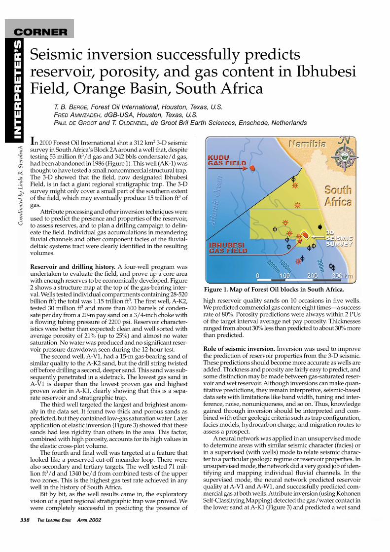
In 2000 Forest Oil International shot a 312 km2 3-D seismicsurvey in South Africa’s Block 2Aaround a well that, despitetesting 53 million ft3/d gas and 342 bbls condensate/d gas,had been abandoned in 1986 (Figure 1). This well (AK-1) wasthought to have tested a small noncommercial structural trap.The 3-D showed that the field, now designated IbhubesiField, is in fact a giant regional stratigraphic trap. The 3-Dsurvey might only cover a small part of the southern extentof the field, which may eventually produce 15 trillion ft3 ofgas.

Attribute processing and other inversion techniques wereused to predict the presence and properties of the reservoir,to assess reserves, and to plan a drilling campaign to delin-eate the field. Individual gas accumulations in meanderingfluvial channels and other component facies of the fluvial-deltaic systems tract were clearly identified in the resultingvolumes.

Reservoir and drilling history. A four-well program wasundertaken to evaluate the field, and prove up a core areawith enough reserves to be economically developed. Figure2 shows a structure map at the top of the gas-bearing inter-val. Wells tested individual compartments containing 28-520billion ft3; the total was 1.15 trillion ft3. The first well, A-K2,tested 30 million ft3 and more than 600 barrels of conden-sate per day from a 20-m pay sand on a 3/4-inch choke witha flowing tubing pressure of 2200 psi. Reservoir character-istics were better than expected: clean and well sorted withaverage porosity of 21% (up to 25%) and almost no watersaturation. No water was produced and no significant reser-voir pressure drawdown seen during the 12-hour test.

The second well, A-V1, had a 15-m gas-bearing sand ofsimilar quality to the A-K2 sand, but the drill string twistedoff before drilling a second, deeper sand. This sand was sub-sequently penetrated in a sidetrack. The lowest gas sand inA-V1 is deeper than the lowest proven gas and highestproven water in A-K1, clearly showing that this is a sepa-rate reservoir and stratigraphic trap.

The third well targeted the largest and brightest anom-aly in the data set. It found two thick and porous sands aspredicted, but they contained low-gas saturation water. Laterapplication of elastic inversion (Figure 3) showed that thesesands had less rigidity than others in the area. This factor,combined with high porosity, accounts for its high values inthe elastic cross-plot volume.

The fourth and final well was targeted at a feature thatlooked like a preserved cut-off meander loop. There werealso secondary and tertiary targets. The well tested 71 mil-lion ft3/d and 1340 bc/d from combined tests of the uppertwo zones. This is the highest gas test rate achieved in anywell in the history of South Africa.

Bit by bit, as the well results came in, the exploratoryvision of a giant regional stratigraphic trap was proved. Wewere completely successful in predicting the presence of

high reservoir quality sands on 10 occasions in five wells.We predicted commercial gas content eight times—a successrate of 80%. Porosity predictions were always within 2 PUsof the target interval average net pay porosity. Thicknessesranged from about 30% less than predicted to about 30% morethan predicted.

Role of seismic inversion. Inversion was used to improvethe prediction of reservoir properties from the 3-D seismic.These predictions should become more accurate as wells areadded. Thickness and porosity are fairly easy to predict, andsome distinction may be made between gas-saturated reser-voir and wet reservoir. Although inversions can make quan-titative predictions, they remain interpretive, seismic-baseddata sets with limitations like band width, tuning and inter-ference, noise, nonuniqueness, and so on. Thus, knowledgegained through inversion should be interpreted and com-bined with other geologic criteria such as trap configuration,facies models, hydrocarbon charge, and migration routes toassess a prospect.

Aneural network was applied in an unsupervised modeto determine areas with similar seismic character (facies) orin a supervised (with wells) mode to relate seismic charac-ter to a particular geologic regime or reservoir properties. Inunsupervised mode, the network did a very good job of iden-tifying and mapping individual fluvial channels. In thesupervised mode, the neural network predicted reservoirquality at A-V1 and A-W1, and successfully predicted com-mercial gas at both wells. Attribute inversion (using KohonenSelf-Classifying Mapping) detected the gas/water contact inthe lower sand at A-K1 (Figure 3) and predicted a wet sand

338 THE LEADING EDGE APRIL 2002 APRIL 2002 THE LEADING EDGE 0000

Seismic inversion successfully predictsreservoir, porosity, and gas content in IbhubesiField, Orange Basin, South Africa

T. B. BERGE, Forest Oil International, Houston, Texas, U.S.FRED AMINZADEH, dGB-USA, Houston, Texas, U.S.PAUL DE GROOT and T. OLDENZIEL, de Groot Bril Earth Sciences, Enschede, Netherlands

INTE

RP

RE

TE

R’S

CORNERC

oord

inat

ed b

y Li

nda

R. S

tern

bach

Figure 1. Map of Forest Oil blocks in South Africa.

at A-W1. Unfortunately, this work was not completed untilafter A-W1 had been drilled.

Most examples in this paper are from cross-lines of the3-D survey that tie A-K1, the discovery well for IbhubesiField. Figure 4 is a log display from the reservoir interval inA-K1. Many forward models have been done of this welland of all wells in the field. The well contains good inver-sion targets including resolvable gas sands—the “upper” and“middle” sands (although there are actually two pressurecompartments in the upper sand with thin perched water).Other targets are a thin and usually unresolvable water sandand a thick, resolvable gas sand with a gas/water contact init.

An inversion is an attempt to predict rock properties(porosity, thickness, fluid content, hydrocarbon saturation,etc.) from seismic data. There are three fundamental types—acoustic, elastic, and attribute. Each has different require-ments for data input and differ in their predictive capability.The right inversion to use depends primarily on the data andan area’s stage of exploration or development.

When we talk about inversion as a specific process, usu-ally we mean a numerical process that uses the seismicresponse to predict rock properties such as velocity, density,compressibility, porosity, and water saturation. An array ofmethodologies claim to be able to do this.

The seismic method measures only four fundamentalrock-physics properties: P-wave velocity, S-wave velocity,density, and anisotropy. Only the first three properties aremeasured with the accuracy required for inversion. Invertingseismic data to other rock properties implicitly assumes arelationship between the property and one or more of thesefundamental properties. All types of inversion require some

form of constraint and need to be calibrated by tying the resultto real or simulated well data. In this paper, we group pop-ular inversion methods into: acoustic, elastic, and attributeinversion (Table 1).

In an exploration setting where little or no well controlis available, a simple acoustic inversion may be best. Duringfield development, when there is a lot of well control, anattribute inversion will be more useful.

In our acoustic inversion, the seismic data were trans-formed into a recursive inversion solution for porosity. A90°phase shift occurs when the data are inverted. The event isshifted so that the peak corresponds to the bed instead of itsboundaries. The volume can then be scaled for porosity andcalibrated by well control. Figure 5 shows examples fromIbhubesi Field. We predicted unusually high (average 21%)porosity at A-Y1 using these same data. This was confirmedby drilling.

Some recursive methods allow input from geologic mod-els and well control to constrain the inversion. Anothersophisticated approach involves solving the three-termBortfeld equation (Bortfeld, 1989). This can be considered anacoustic method because it solves for VP, VS, and density but


Figure 3. 3-D perspective of a cross-line through A-K1looking east that shows the resulting Kohonen shape-attribute results. Green = pay; yellow = wet sand. Notetransition from pay to wet. This corresponds to thegas/water contact in the third sand in A-K1. The twoclasses were then seeded through the volume. Red bodyis the gas pay class and the blue is the wet sand class.Note that the contact between the classes consist of twoflat segments and that the gas class always overlies thewet class—compelling evidence that we are actuallyimaging a gas/water contact.

Figure 2. Structure map on the top of the gas-bearinginterval showing well A-K1 well and subsequent wellsA-K2, A-V1, A-W1, and A-Y1. Note lack of structuralclosure for A-K1. Mapped from a 3-D depth volume. CI= 20. Datum is sea level.

Table 1. Grouping of popular inversion methodsMethodAcoustic

Elastic

Attribute

ResultsSolves for Density and VelocitySolves forCompressibility,Shear Strength,and RigidityUses waveshapes, seismiccharacters or derived features

Input NeededOnly stacked P-Wave

Shear or Gather data

Any form of seismic,Acoustic/ElasticImpedance

PredictsPorosity,ThicknessPorosity,ThicknessLithology,Sw?Porosity,ThicknessLithology,Sw?

is not recursive. The terms of the equation represent theintercept, gradient, and curvature of the offset amplitudes.By solving for density, wet and gas-bearing sands might bedistinguished. The method requires preservation of trueamplitudes, offset angles out to the critical angle if possible,and good quality, low-noise data.

More input is required but more predictive output canbe obtained by doing an elastic inversion. Elastic inversionrequires shear-wave information. If directly recorded shear-wave information is not available, it can be estimated in anumber of ways based on AVO and P-wave data using somesimplified form of the Zoeppritz equations, Shuey’s equa-tion, or a Castagna relationship.

Figure 6 is an example of an elastic inversion based ona P-wave, S-wave crossplot method. This was the primaryvolume used to site wells for the 2000-2001 drilling campaignin Ibhubesi Field. Ten reservoir predictions were made onthe basis of this volume. All found porous reservoir and 8(80% COS) found gas.

The goal of attribute inversion is to visualize seismic pat-terns pertaining to a specific geologic interval. An unsuper-vised neural network performs this task by clustering seismicwaveforms around a mapped horizon. Input to the neuralnetwork is a set of seismic amplitudes. The number of seg-ments and the time-gate relative to the mapped horizon areuser-defined parameters. Each segment is characterized bya waveform-shaped class center (Figure 7). The network firsthas to learn how to segment the seismic waveforms. Thistraining is done on a representative selection of seismicwaveforms. A training set is created by regular sampling atevery tenth in-line and cross-line.

The supervised approach requires a representative dataset. We train the network by feeding it examples from therepresentative data set (the training set). The neural networkthen learns how the input data is related to the desired out-put. The supervised approach is a form of nonlinear, multi-variate regression that is used to quantify or classify data.Examples of quantification are networks that predict, fromthe seismic response, such properties as porosity or pore vol-ume. Popular supervised learning networks are multilayerperceptrons (MCP) and radial basis functions networks (deGroot, 1995).

In the unsupervised approach, the aim is to find struc-ture in the data themselves, without imposing an a-priori


Figure 4. Log display of pay interval in A-K1, DSTresults, and inversion objectives.

Figure 5. (a)Conventional P-wavefrom the 3-D survey withA-K1 well tie. (b)Recursive inversion ofthe line in Figure 5a.Note that events havebeen phase-shifted 90°and that amplitudes areall positive and in impe-dence units. (c) Sectionfrom Figure 5b scaled inporosity units.

a)

b)

c)

Figure 6. A 300-m volume rendering of an elastic inver-sion showing the five wells in Ibhubesi Field and thereservoir anomalies they penetrated. A-K1 is the Soekorwell drilled in 1986. Forest Oil wells are A-K2, A-V1, A-W1, and A-Y1, drilled in that respective order in 2000-2001. Only A-W1 was wet.

conclusion. Unsupervised learning is used for data seg-mentation—i.e., data clustering (Figure 8). The resultingsegments (e.g., clusters of similar seismic waveforms at thereservoir level) remain to be interpreted. Popular networksthat use unsupervised learning are the unsupervised vec-tor quantifier (de Groot, 1995) and Kohonen feature maps(e.g., Lippmann, 1989).

In interpreting neural network patterns, one mustaccount for the fact that the seismic response is smearedacross overlying and underlying sequences. Response fromsome units may interfere with those from other levels. Ifthe stratigraphic intervals are not parallel, the extractionwindow cuts through the underlying or overlying geol-ogy, and the results become difficult to interpret. However,even with these limitations, we can still extract valuablegeologic and petrophysical information from observedpatterns. A qualitative interpretation can be based on geo-logic insight. A more quantitative interpretation involvesanalyzing the seismic waveforms of each segment in termsof geologic/petrophysical variations using real and sim-ulated wells.

Pseudo wells. Adding pseudo wells can increase the sta-tistical database for training a neural network. Pseudowells, which simulate the results of drilling, have well logsbut no spatial locations. They can be used to quantifywaveform segmentation results (also known as seismic

facies maps). In this case study,they were used to create the repre-sentative learning set for a super-vised neural network. Thesimulation is based on a con-strained Monte Carlo procedureand is built around an integrationframework, a hierarchical descrip-tion of the subsurface units. In thisstudy, pseudo wells were neededbecause only three actual wells hadbeen drilled at the start of the pro-ject.

The seismic input for networktraining came from synthetic seis-mic (near- and mid-offset) andacoustic impedance traces of 40pseudo wells. Seismic waveformsof [-20,20] ms length for near- andmid-offset were extracted relativeto a reference time, sliding with 4-ms steps. The amplitude of the syn-thetic impedance trace at thesliding reference time serves as anadditional input node to the neuralnetwork. Figure 9 shows the neuralnetwork topology for the porosityprediction. The output consistedof the amplitude of either theporosity trace or the pay flag trace.The variable called pay flag is sim-

ulated as a Boolean variable (1 indicates gas-filled sand and0 indicates brine-filled sand or shale).

Both were constructed by converting the depth curveto two-way time using the velocity log. The time curve wassubsequently resampled with an antialias filter to 4-mssampling.

In Table 2, the performance is shown for the gas prob-ability prediction to monitor the neural network duringtraining and to stop training before overfitting sets in.Overfitting occurs when the network loses its generaliza-tion ability. To avoid overfitting, the two actual wells wereused as test data during the training of the network.

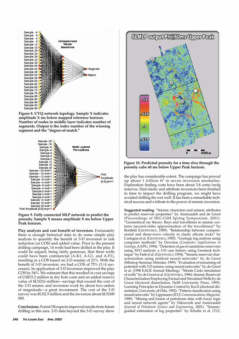
The trained networks were applied to the seismic andimpedance cube every 4 ms in a time slice of 0-250 ms rel-ative to the mapped upper peak horizon, yielding a poros-ity and pay flag prediction cube. Figure 9 shows fullyconnected MLP network to predict the porosity, and Figure10 shows a slice through the porosity cube 60 ms belowthe Upper Peak horizon. Figure 11 is an in-line throughthe gas probability cube. The closer the value is to 1 orhigher, the more likely it is that we are dealing with gas-filled sand. As such the output can be considered to rep-resent the gas sand probability.

To validate the inversion method, the network wasapplied to real wells AK-1 and AG-1. Because the real welldata were not used to train the neural network, the realwells are blind test locations. Figure 12 shows the resultfor pay flag. Each plot shows two curves: the actual payflag trace in pink and the trace predicted by the neural net-work in blue. From the predictions on well logs it can beobserved that, in general, the neural network is quite capa-ble of transforming acoustic and elastic properties into thetarget gas probability response. Note the blue curve is notthe actual gas probability but the predicted likelihood notscaled to 1. The same applies to the porosity inversion.


Table 2. Neural network performance for gas probability

43.13 %7.26 %

50.40 %

6.86 %42.74 %49.60 %

50 %50 %Total misclassified14.12 %

5.88 %9.80 %

15.69 %

0.98 %83.33 %84.13 %

6.8693.14Total misclassified10.87 %

Train data (balanced) Test data (AK-1, AG-1)

Figure 7. Results for UVQ analysis over time gate [-4,96] relative to Upper Peakhorizon.

Play analysis and cost benefit of inversion. Fortunatelythere is enough historical data to do some simple playanalysis to quantify the benefit of 3-D inversion in riskreduction (or COS) and added value. Prior to the presentdrilling campaign, 14 wells had been drilled in the play. Itcould be argued, being fairly generous, that three wellscould have been commercial (A-K1, A-G1, and A-F1),resulting in a COS based on 2-D seismic of 21%. With thebenefit of 3-D inversion, we had a COS of 75% (3/4 suc-cesses). So application of 3-D inversion improved the playCOS by 54%. We estimate that this resulted in cost savingsof US$15.2 million in dry hole costs and an added reservevalue of $US216 million—savings that exceed the cost ofthe 3-D seismic and inversion work by about two ordersof magnitude—a great investment. The cost of the 3-Dsurvey was $US2.5 million and the inversion about $US300000.

Conclusions. Forest Oil expects improved results from futuredrilling in this area. 2-D data beyond the 3-D survey show

the play has considerable extent. The campaign has provedup about 1 trillion ft3 in seven inversion anomalies.Exploration finding costs have been about 3.8 cents/mcfgreserves. Had elastic and attribute inversions been finishedin time to impact the drilling program, we might haveavoided drilling the wet well. It has been a remarkable tech-nical success and a tribute to the power of seismic inversion.

Suggested reading. “Seismic characters and seismic attributesto predict reservoir properties” by Aminzadeh and de Groot(Proceedings of SEG-GSH Spring Symposium, 2001).“Geometrical ray theory: Rays and traveltimes in seismic sys-tems (second-order approximation of the traveltimes)” byBortfeld (GEOPHYSICS, 1989). “Relationship between compres-sional and shear-wave velocity in clastic silicate rocks” byCastagna et al. (GEOPHYSICS, 1985). “Geologic log analysis usingcomputer methods” by Doveton (Computer Applications inGeology, AAPG, 1994). “Detection of gas in sandstone reservoirsusing AVO analysis: a 3-D case history using Geostack tech-nique” by Fatti et al. (GEOPHYSICS, 1994). “Seismic reservoir char-acterization using artificial neural networks” by de Groot(Mintrop Seminar, Münster, 1999). “Evaluation of remaining oilpotential with 3-D seismic using neural networks” by de Grootet al. (1998 EAGE Annual Meeting). “Monte Carlo simulationof wells” by de Groot et al. (GEOPHYSICS, 1996). Seismic ReservoirCharacterization Employing Factual and Simulated Wells by deGroot (doctoral dissertation, Delft University Press, 1995).Learning Principles in Dynamic Control by Kavli (doctoral dis-sertation, University of Oslo, 1992). “Pattern classification usingneural networks” by Lippmann (IEEE Communications Magazine,1989). “Mining and fusion of petroleum data with fuzzy logicand neural network agents” by Nikravesh and Aminzadeh(Journal of Petroleum Science and Engineering, 2001). “Seismic-guided estimation of log properties” by Schultz et al. (TLE,


Figure 8. UVQ network topology. Sample X indicatesamplitude X ms below mapped reference horizon.Number of nodes in middle layer indicates number ofsegments. Output is the index number of the winningsegment and the “degree-of-match.”

Figure 9. Fully connected MLP network to predict theporosity. Sample X means amplitude X ms below UpperPeak horizon.

Figure 10. Predicted porosity for a time slice through theporosity cube 60 ms below Upper Peak horizon.

1994). “A simplification of the Zoeppritz equations” by Shuey(GEOPHYSICS, 1985). LE

Timothy B. Swearingen Berge is chief geo-physicist with Forest Oil International withexploration ventures in Romania, Italy,Switzerland, Bavaria, Thailand, Sicily, Tunisia,and offshore RSA. He worked for 17 years withExxon in Denver; Midland; Bogota, Colombia;and Houston. Berge has a BS in geology and geo-physics (1976) from the University of Wisconsin,Madison and MA (1981) from the Universityof Texas at Austin. He has served as the AfricaRegional Coordinator and currently chairs

SEG’s Global Affairs Committee.

Fred Aminzadeh is president and CEO of dGB-USA of Houston, Texas, U.S. The firm special-izes in services and software for quantitativeseismic interpretation, stratigraphic analysis, seis-mic inversion, neural networks-based reservoircharacterization and anomaly (chimneys, faultand fracture) detection. Aminzadeh previouslyworked for Unocal. He has published extensivelyon reservoir characterization, seismic attributes,AVO modeling, pattern recognition, artificialintelligence, and neural networks. He has chaired

SEG’s Research Committee and was vice chairman of the Global AffairsCommittee. He is currently SEG vice president.

Paul de Groot is managing director of dGB, whichspecializes in quantitative seismic interpretation,stratigraphic analysis, seismic inversion, neuralnetworks-based reservoir characterization andchimney/fracture detection. He worked 10 yearsfor Shell in various technical and managementpositions and four years as a senior research geo-physicist for TNO before cofounding dGB in 1995.He holds MSc and PhD degrees in geophysics fromthe Delft University of Technology.

Tanja Oldenziel, a geoscientist with dGB, theNetherlands, is involved in a variety of seismicreservoir characterization projects. She received apetroleum engineering degree from DelftUniversity of Technology (1997) and is pursuinga PhD on “The use of time-lapse seismic withinreservoir engineering.”

Corresponding author: [email protected] or [email protected]


Figure 12. Gas probability as predicted by MLP neuralnetwork (blue) plotted against actual pay flag (pink) inAK-1 (top) and AG-1 (bottom). The curves for AG-1 donot align perfectly due to a small time shift.

Figure 11. Predictedgas probability forin-line 2463. Blackline is Upper Peakhorizon. AK-1 wasdrilled at cross-line3181.

CORNER Seismic inversion successfully predicts … · Seismic inversion successfully predicts...

Documents

Transcript of CORNER Seismic inversion successfully predicts … · Seismic inversion successfully predicts...