core.ac.uk · AfastIMPESmultiphaseflowsolverinporousmediafor reservoirsimulation Abstract In this...
114
UNIVERSIDAD POLITÉCNICA DE MADRID ESCUELA TÉCNICA SUPERIOR DE INGENIEROS AERONÁUTICOS A fast IMPES multiphase flow solver in porous media for reservoir simulation Doctoral Thesis By Carlos Redondo Calle Aeronautical Engineer June 2017
Transcript of core.ac.uk · AfastIMPESmultiphaseflowsolverinporousmediafor reservoirsimulation Abstract In this...

UNIVERSIDAD POLITÉCNICA DE MADRIDESCUELA TÉCNICA SUPERIOR DE INGENIEROS AERONÁUTICOS
A fast IMPES multiphase flow solver inporous media for reservoir simulation
Doctoral Thesis
By
Carlos Redondo CalleAeronautical Engineer
June 2017


Departamento de Matemática Aplicada y EstadísticaEscuela Técnica Superior de Ingenieros Aeronáuticos
A fast IMPES multiphase flow solver inporous media for reservoir simulation
by
Carlos Redondo CalleAeronautical Engineer
Advisors:
Eusebio Valero SánchezPh.D. in Aeronautical Engineering
Gonzalo Rubio CalzadoPh.D. in Aeronautical Engineering
Madrid, June 2017

This thesis has been partially supported by Repsol.S.A underthe research grant P130120150.
Esta tesis ha sido cofinanciada por Repsol.S.A en el marcodel proyecto de investigación P130120150.

El tribunal nombrado por el Sr. Rector Magnífico de la Universidad Politécnica deMadrid, el día ............ de .................. de 20......
Presidente:
Vocal:
Vocal:
Vocal:
Secretario:
Suplente:
Suplente:
Realizado el acto de defensa y lectura de la Tesis el día ........ de ................ de 20....en la E.T.S.I./Facultad.........................................
Calificación...............................
EL PRESIDENTE LOS VOCALES
EL SECRETARIO


A fast IMPES multiphase flow solver in porous media forreservoir simulation
AbstractIn this thesis, a methodology to efficiently solve the multiphase flow through a porousmedia in the near wellbore region is presented. The mathematical models, the nu-merical methods and practical implementation details for a functional 2D solver arepresented.
The methods described in this thesis are the base of an industrial 3D code. Thus,many efforts have been made to validate all the new models to guarantee robustnessand stability in the solution without penalising the efficiency.
The numerical discretisation is based on the IMplicit Pressure Explicit Saturation(IMPES) approach. While most of the works in the literature rely on Fully ImplicitMethods (FIM) to simulate the reservoir scale, this is not suited, in general, for thenear wellbore region, where smaller computational and physical times are required,therefore parametric history matching models are preferred to solve this region. How-ever, parametric models present several uncertainties that can affect significantly theestimation of the pressure drop. An accurate and fast simulation of that region istherefore required.
Here, a novel and robust implementation of the IMPES scheme is presented, aimingto reduce the large computational cost of the (implicit) pressure equations and toincrease the robustness and reliability of the scheme. The method takes advantageof the short physical time steps between iterations, imposed by the explicit saturationsolver, to produce a new pressure field at the numerical cost of an explicit schemeusing an iterative solver. One, two and three-dimensional numerical experiments arecarried out to show the validity of the proposed discretisation. It is shown that thecost of the method is reduced an order of magnitude when compared to the classicalIMPES, which outperforms, in a lot of scenarios, the state of the art of current implicitmethods.
Keywords: Porous media, multiphase flow, reservoir simulation, IMPES, iterativemethods.
v

A fast IMPES multiphase flow solver in porous media forreservoir simulation
ResumenEn esta tesis se propone una nueva metodología para resolver, de forma eficiente,el flujo multifásico en medio poroso para la región próxima a las perforaciones enyacimientos de hidrocarburos (near–wellbore). En este trabajo se presentan los mo-delos matemáticos, los métodos numéricos y detalles prácticos de la implementaciónpara un simulador 2D.
Los métodos descritos en esta tesis han servido como base para un simulador 3Dindustrial, por lo tanto, los principales esfuerzos se han dedicado a la validación delos nuevos modelos para garantizar la estabilidad y la robustez del método sin que laeficiencia se vea afectada.
La discretización numérica está basada en el método IMPES (Implicit Pressure Ex-plicit Saturation), en el cual, el problema asociado a la presión se trata de formaimplícita mientras que el problema asociado a la saturación se resuelve de forma ex-plícita. La mayoría de códigos presentes en la literatura utilizan métodos totalmenteimplícitos o Fully Implicit Methods (FIM) para la simulación de yacimientos. Estosmétodos no son, en general, apropiados para la región cercana al pozo donde se nece-sitan pasos temporales más reducidos. En esta región se usan modelos paramétricosbasados en datos históricos. Estos métodos presentan incertidumbres que puedenafectar de forma significativa a la estimación de la distribución de presión. Por con-siguiente, es necesario un método para simular de forma precisa y eficiente el flujo enesta región.
En esta tesis se presenta una implementación novedosa del esquema IMPES. Sereduce el coste computacional asociado a las ecuaciones de presión (parte implícita) yse mantiene la estabilidad del esquema. El método se aprovecha de los pasos tempo-rales reducidos, impuestos por la ecuación de saturación, para actualizar el campo depresión por el coste numérico de una iteración explícita utilizanto un método iterativo.La discretización propuesta se ha validado con con experimentos numéricos en una,dos y tres dimensiones. Se demuestra, además, que el método propuesto reduce enun orden de magnitud el tiempo computacional de las implementaciones clásicas delIMPES y mejora, en numerosos escenarios, el rendimiento de los métodos implícitos.
Keywords: Medio poroso, flujo multifásico, simulación de yacimientos, IMPES,métodos iterativos.
vi

Acknowledgements
First, I would like to thank my advisors, Eusebio Valero and Gonzalo Rubio, fortheir support and encouragement during this thesis. I also would like to thank ÁngelRivero for for the coordination of the project that has led to this thesis and his helpand interesting discussions during my time in the Centro de Tecnología de Repsol.
I would like to thank the Applied Mathematics Department for the incredible workenvironment during the stays at the University.
I also want to thank my family, my friends and especially Araceli, without whomthis PhD would have never been possible.
Finally, I want to thank to Repsol that has funded this doctoral thesis under theresearch grant P130120150.
vii

Agradecimientos
Primero, me gustaría agradecer a mis tutores de tesis, Eusebio Valero y GonzaloRubio por su apoyo y ánimos durante el desarrollo de esta tesis. Me gustaría agradecertambién a Ángel Rivero por la coordinación del proyecto que ha dado lugar a estatesis y por su ayuda e interesantes discusiones durante mis estancias en el Centro deTecnología de Repsol.
Quiero agradecer también al Departamento de Matemática Aplicada por el fabu-loso ambiente de trabajo en mi estancia en la Universidad.
También quiero dar las gracias a mi familia y amigos, en especial a Araceli, sin loscuales este doctorado no habría sido posible.
Por último, agradecer a Repsol por la financiación de esta tesis, en el marco delproyecto de investigación P130120150.
viii

CONTENTS
1 Introduction 11.1 The problem of reservoir simulation . . . . . . . . . . . . . . . . . . . . . . 11.2 Motivation . . . . . . . . . . . . . . . . . . . . . . . . . . . . . . . . . . . . . 21.3 Methodology . . . . . . . . . . . . . . . . . . . . . . . . . . . . . . . . . . . . 4
2 Mathematical Models 72.1 The porous media . . . . . . . . . . . . . . . . . . . . . . . . . . . . . . . . . 7
2.1.1 Continuum approach . . . . . . . . . . . . . . . . . . . . . . . . . . 82.1.2 Properties of porous media . . . . . . . . . . . . . . . . . . . . . . . 9
2.2 Flow in porous media . . . . . . . . . . . . . . . . . . . . . . . . . . . . . . 112.2.1 Darcy’s law . . . . . . . . . . . . . . . . . . . . . . . . . . . . . . . . 112.2.2 Validity of Darcy’s law . . . . . . . . . . . . . . . . . . . . . . . . . . 132.2.3 Single–phase flow . . . . . . . . . . . . . . . . . . . . . . . . . . . . 14
2.3 Multi–phase flow in porous media . . . . . . . . . . . . . . . . . . . . . . . 152.3.1 Immiscible two–phase flow . . . . . . . . . . . . . . . . . . . . . . 152.3.2 Relative permeability . . . . . . . . . . . . . . . . . . . . . . . . . . 172.3.3 Capillary pressure . . . . . . . . . . . . . . . . . . . . . . . . . . . . 202.3.4 Immiscible incompressible two–phase flow problem . . . . . . . 23
3 Numerical Methods 253.1 Spatial discretisation . . . . . . . . . . . . . . . . . . . . . . . . . . . . . . . 25
Scheme order . . . . . . . . . . . . . . . . . . . . . . . . . . . . . . . 293.1.1 Boundary conditions . . . . . . . . . . . . . . . . . . . . . . . . . . 29
Pressure inflow / outflow . . . . . . . . . . . . . . . . . . . . . . . . 30Flow . . . . . . . . . . . . . . . . . . . . . . . . . . . . . . . . . . . . 30Wells . . . . . . . . . . . . . . . . . . . . . . . . . . . . . . . . . . . . 30
3.1.2 Mesh refinement . . . . . . . . . . . . . . . . . . . . . . . . . . . . . 323.2 Temporal discretisation . . . . . . . . . . . . . . . . . . . . . . . . . . . . . 333.3 Iterative pressure solver . . . . . . . . . . . . . . . . . . . . . . . . . . . . . 34
ix

x CONTENTS
3.3.1 FGMRES(m) . . . . . . . . . . . . . . . . . . . . . . . . . . . . . . . 35Preconditioners . . . . . . . . . . . . . . . . . . . . . . . . . . . . . . 36
3.3.2 Iterative solver tolerance . . . . . . . . . . . . . . . . . . . . . . . . 38
4 Numerical Experiments and Validation 414.1 Validation cases . . . . . . . . . . . . . . . . . . . . . . . . . . . . . . . . . . 41
4.1.1 Case 1. Buckley-Leverett problem. . . . . . . . . . . . . . . . . . . 424.1.2 Case 2. SPE10 dataset 1 . . . . . . . . . . . . . . . . . . . . . . . . 444.1.3 Case 3. Banded plug . . . . . . . . . . . . . . . . . . . . . . . . . . . 474.1.4 Case 4. Heterogeneous plug . . . . . . . . . . . . . . . . . . . . . . 494.1.5 Case 5. Five–spot . . . . . . . . . . . . . . . . . . . . . . . . . . . . 554.1.6 Case 6. SPE10 dataset 2 . . . . . . . . . . . . . . . . . . . . . . . . 59
4.2 Analysis of iterative solver . . . . . . . . . . . . . . . . . . . . . . . . . . . . 614.2.1 Impact of preconditioner . . . . . . . . . . . . . . . . . . . . . . . . 614.2.2 GMRES restart . . . . . . . . . . . . . . . . . . . . . . . . . . . . . . 63
5 Multiphase 2D IMPES Solver 655.1 Input/Output files . . . . . . . . . . . . . . . . . . . . . . . . . . . . . . . . . 66
5.1.1 File format . . . . . . . . . . . . . . . . . . . . . . . . . . . . . . . . . 665.2 Implementation methodology . . . . . . . . . . . . . . . . . . . . . . . . . 67
5.2.1 Sparse matrix storage . . . . . . . . . . . . . . . . . . . . . . . . . . 705.2.2 Parallelisation . . . . . . . . . . . . . . . . . . . . . . . . . . . . . . . 71
Conclusions 75
Appendices 77
A Data structure. AOS vs SOA 79
B Fortran – Python plotting 87

NOMENCLATURE
Acronyms
bbl Barrels of oil (0.1589873m3)
CG Conjugate Gradient
CSR Compressed Sparse Storage
EOS Enhaced Oil Recovery
FIM Fully Implicit Methods
GMRES Generalised Minimal Redis-ual
HPC High Performance Comput-ing
ILU Incomplete LU factoriza-tion
IMEX Implicit Explicit Method
IMPES Implicit Pressure ExplicitSaturation
LHS Left Hand Side
NZ Non–zero pattern
PV Pore Volume
PVI Pore Volume Injected
REV representative elementaryvolume
RHS Right Hand Side
RK Runge Kutta
SOR Successive Overrelaxation
SI International System ofUnits
SSOR Symmetric SuccessiveOverrelaxation
SPE Society of Petroleum Engi-neers
TVD Total Variation Diminishing
VTK Visualization Tool Kit
Greek Symbols
∆t Time step
∆Smax Maximun saturation varia-tion per time step
ϕ Slope limiter function
γ Surface tension
λ Phase mobilityPorosity distribution index
µ Dynamic viscosity
ν Kinematic viscosity
φ Porosity
ρ Density
θ Contact angle
xi

xii CONTENTS
Roman Symbols
A Discretized pressure equa-tion system matrix
A Cross sectional area
b Right hand side in pressureequation
Bc Logarithmic capillary pres-sure model constant
c Compressibility
DIVer ror Error in divergence of totalvelocity per time step
fw Wetting phase fractionalflow
f ′w Derivative of the wettingphase fractional flow
g Gravity vector
g Gravitational contant
I Identity matrix
J J–Leverett functionProductivity index
K Permeability tensor
k Absolute permeability
kr Relative permeability
ki Effective permeability ofphase i
m, n Brooks–Corey exponents
p Vector of unknowns in pres-sure equation
p Pressure
pc,0 Capillary entry pressure
pc Capillary pressure
Q Flow rate
q Volumetric flow
q Mass flow rate
r Radius of curvature
Re Reynolds number
rw Wellbore radius
r0 Peacemann equivalentwellbore radius
s, S Phase saturation
Se f f Effective saturation
Si,r Irreducible (connate) satu-ration of phase i
T Intercell transmissibility
t Time
u Darcy velocity, velocity
u Velocity vector
x Spatial corrdinates vector
Superscriptsn Time step n–th
Subscripts
i Generric phase i
n Non wetting phase
r Relative to rock or porousmatrix
w Water or wetting phase
x x direction
y y direction

LIST OF FIGURES
2.1 Schematic of two immiscible phases on porous media at microscopicscale. . . . . . . . . . . . . . . . . . . . . . . . . . . . . . . . . . . . . . . . . . 8
2.2 (a): Accurate rock structure representation using rock Micro-CT.(b): Simplified porous representations.(c) Continuum approach to porous media. . . . . . . . . . . . . . . . . . 9
2.4 Darcy’s experiment . . . . . . . . . . . . . . . . . . . . . . . . . . . . . . . . 122.5 Schematic streamlines in porous media . . . . . . . . . . . . . . . . . . . . 132.6 (a): Typical relative permeability curves for the oil–water system.
(b): Hysteresis on relative permeability curves. . . . . . . . . . . . . . . . 182.7 Comparative between Brook–Corey and Van Genuchten relative perme-
ability correlations. . . . . . . . . . . . . . . . . . . . . . . . . . . . . . . . . 202.8 Hysteresis in capillary pressure curves. . . . . . . . . . . . . . . . . . . . . 212.9 Comparative between Brooks–Corey and Van Genuchten models for
capillary pressure correlation. . . . . . . . . . . . . . . . . . . . . . . . . . 22
3.1 Five-point finite differences stencil on a staggered grid. . . . . . . . . . . 263.2 TVD limiter functions. . . . . . . . . . . . . . . . . . . . . . . . . . . . . . . 283.3 Impact of the flux limiter in the solution of the Buckley-Leverett problem. 293.4 Solutions used for scheme order estimation using Richardson extrapo-
lation. . . . . . . . . . . . . . . . . . . . . . . . . . . . . . . . . . . . . . . . . 303.5 Stencil used in face and corner boundaries. . . . . . . . . . . . . . . . . . 313.6 Impact of mesh refinement in the solution. . . . . . . . . . . . . . . . . . 323.7 Evolution of the GMRES tolerance, pressure error and total divergence
error with the number of GMRES iterations. . . . . . . . . . . . . . . . . . 393.8 Evolution of GMRES and divergente tolerance error. . . . . . . . . . . . 40
4.1 Case 1. Water saturation profiles for the Buckley–Leverett solution. . . 434.2 Case 2. Absolute permeability field and gas saturation distributions. . . 454.3 Case 2. Error in saturation distribution with gravity. . . . . . . . . . . . . 45
xiii

xiv LIST OF FIGURES
4.4 Case 2. Error in saturation distribution with no gravity. . . . . . . . . . . 464.5 Case 2. Gas production history. . . . . . . . . . . . . . . . . . . . . . . . . . 464.6 Case 2. Iterative solver efficiency. . . . . . . . . . . . . . . . . . . . . . . . 474.7 Case 3. Absolute permeability and wetting phase saturation distribution. 484.8 Case 3. Error distribution for different tolerance values. . . . . . . . . . 494.9 Case 3. Iterative solver efficiency. . . . . . . . . . . . . . . . . . . . . . . . 504.10 Case 4a. Permeability and wetting phase distribution. . . . . . . . . . . 514.11 Case 4a. Error distribution for different values of solver tolerance. . . . 514.12 Case 4b. Permeability and wetting phase distribution. . . . . . . . . . . 524.13 Case 4b. Error distribution for different values of solver tolerance. . . . 524.14 Case 4a. Permeability and wetting phase distribution. . . . . . . . . . . 534.15 Case 4c. Error distribution for different values of solver tolerance. . . . 544.16 Case 4. Efficiency of iterative solver for different tolerances. . . . . . . . 544.17 Case 5. Absolute permeability and water distribution. . . . . . . . . . . 564.18 Case 5. Finger structure for different solver tolerances. . . . . . . . . . 574.19 Case 5. Impact of solver tolerance. . . . . . . . . . . . . . . . . . . . . . . 584.20 Case 6. Permeability distribution for the SPE 10 dataset 2. . . . . . . . 594.21 Case 6. Porosity distribution for the SPE 10 dataset 2. . . . . . . . . . . 604.22 Case 6.Pressure distribution and water distribution. . . . . . . . . . . . 604.23 Case 6. Water cut history. . . . . . . . . . . . . . . . . . . . . . . . . . . . . 614.24 Convergence history for the GMRES linear solver. . . . . . . . . . . . . . 624.25 Impact of preconditioner on the GMRES iterative solver. . . . . . . . . . 624.26 Impact of GMRES restart iteration with ILU(0) preconditioner. . . . . . 634.27 Impact of GMRES restart iteration with ILUT preconditioner. . . . . . . 63
5.1 Rock file visualized with Paraview. . . . . . . . . . . . . . . . . . . . . . . . 685.2 Darcy2D code simplified diagram. . . . . . . . . . . . . . . . . . . . . . . . 695.3 2D solver multithread scalability. . . . . . . . . . . . . . . . . . . . . . . . 73
A.1 AOS and SOA scalability with low arithmetic load loop . . . . . . . . . . 83A.2 AOS and SOA loop memory access profile. . . . . . . . . . . . . . . . . . . 84A.3 AOS and SOA scalability with high arithmetic load loop . . . . . . . . . 85
B.1 Example of Fortran–Python plot . . . . . . . . . . . . . . . . . . . . . . . . 88

chapter 1
INTRODUCTION
1.1 The problem of reservoir simulation
A common misconception in oil and gas recovery processes is that the hydrocarbonsare found in a kind of underground lakes and have to be pumped out of the reser-voir in a similar way water is pumped out of a storage tank. This is absolutely notthe case. Hydrocarbons are found impregnating the void space of porous or fracturedrocks, such as sandstone, carbonates or dolomite. The pores of this kind of rocks areconnected forming a highly irregular microscopic net. The volume of pores is typicallysmall (1–20 %) [Bear, 1972]. The oil or gas impregnating the rock can flow throughthese intricate paths under high pressure differentials. The ability of the rocks topermit the flow of fluids through the pore net varies hugely between different rocktypes, or even between zones of the same rock due to inhomogeneities or fractures.The typical size of the reservoirs, of the order of magnitude of kilometres, and theinfluence of rock inhomogeneities make a hard task to accurately characterize andmodel the porous media [Aarnes et al., 2007]. In addition to the complicated natureof the porous media, the oil or gas are a complex mixture of hydrocarbons, hard tocharacterize, with chemical and physical properties that vary widely between reser-voirs. Initially, the crude oil is at reservoir conditions, at a temperature given by thegeothermal gradient (∼ 30°C/km) and a typical pressure of hundreds of bar. Pres-sure and temperature of the crude oil vary from reservoir to storage conditions duringthe extraction and the physical properties of the hydrocarbon vary during this phaseincluding, often, phase changes.
The pressures found in reservoirs are extremely high, normally these pressures arehigh enough to force the fluids to flow through the porous media and out of the wellswithout much pumping effort. This type of recovery, is named primary recovery. Asthe crude oil is extracted from the reservoir, the pressure drops and the production
1

2 1. Introduction
rate decreases as the gradient driving the flux gets lower. The amount of hydrocar-bons extracted from the reservoir within this type of recovery is typically not greaterthan 30% [Ewing, 1983]. After this phase, a fluid, typically water, is injected in somewells to increase the production rate in the remaining ones. This injection maintainsthe reservoir pressure gradients and the injected fluid displaces the crude towardsthe producers. This phase is known as secondary recovery. Water flooding is a com-plex phenomena, the interface between oil and water is unstable and fingers of theless viscous phase are formed connecting injectors and producers, reducing the effi-ciency of oil displacement. Typically, a 50% of the crude remains in the reservoir afterthis phase [Ewing, 1983]. Other techniques to increase the recovery, known as En-hanced Oil Recovery (EOR) are used in the tertiary recovery phase. The techniquesused in this phase include additives addition to increase the displacement efficiency,gas injection to force miscible displacement, steam injection to reduce oil viscosity orair injection and in-situ combustion for increasing pressure and temperature in thereservoir or even microbial agents injection [Amarnath, 1999]. Physical and chem-ical processes involved in this tertiary phase are complex and extremely difficult toreproduce mathematically.
1.2 MotivationNumerical reservoir simulators are tools widely used by the oil industry and have be-come the main instrument for evaluating recovery efficiency and economical viabilityof new oil-drilling. Simulation of multiphase fluid flow in porous media is currentlya topic of interest in many areas, not only in reservoir simulation, but also in otherfields like hydrology and groundwater flow or waste management.
In reservoir simulation, far-field areas are well-understood and fairly resolved withcurrent simulation tools but near wellbore regions are normally under-resolved andbecome a source of inaccuracy in the resolution of the fluid physics in this zone [Ding,2011; Dumkwu et al., 2012]. The under-resolved physics is modelled by includingseveral parameters, adjusted using history matching, such as the well skin factor or theproductivity index [Dumkwu et al., 2012]. However, the logarithmic pressure drop inthe surrounding wellbore region, as well as the complex thermodynamic behaviourof oil often leads to sudden variations in flow properties. These changes modify theproduction rates in a determinant way and can be hardly predicted by parametricwellbore models. Moreover, new techniques in oil drilling, including crosswise andhorizontal wellbores and enhanced oil recovery techniques, increase the uncertaintiesassociated to these models [Leeftink et al., 2015] making very difficult to accuratelypredict the recovery efficiencies in the mid and long terms. In order to reduce theseuncertainties, it is therefore crucial to accurately simulate the near wellbore region in

1.2 Motivation 3
the most efficient way.
In terms of numerical simulation, the Fully Implicit Method (FIM) [Collins andNghiem, 1992; Dawson et al., 1997; Lee et al., 2011; Sun et al., 2009; Tan and Kaloger-akis, 1991; Wu and Qin, 2009; Yang et al., 2016] and the IMplicit Pressure ExplicitSaturation (IMPES) method [Chen et al., 2004; da Silva et al., 2016; Hurtado et al.,2006; Kou and Sun, 2010a,b; Sheldon et al., 1959; Stone and Garder Jr., 1961] arethe main strategies to solve the system of partial differential equations arising fromthe discretisation of the mathematical model of the multiphase flow in porous media.
The FIM is regularly used in the simulation of the large far-field reservoir areas.Being unconditionally stable, it allows for selecting large time steps which are able tosolve years of operation of complete reservoirs with dozens of producers and injectorsin a few hours of computational time [Künze et al., 2013; Liu et al., 2016]. However,FIM is not well suited for detailed simulation, as required in the near wellbore region,where smaller time steps are needed to capture fast dynamic behaviour and couplingwith pipe simulators. In this region and despite its limitations, the IMPES method isnormally preferred. IMPES is an operator splitting technique [Kou and Sun, 2010b]based on physics, which solves only the pressure equation implicitly, but updates thesaturation explicitly. The pressure equation in this approach is formed by substitut-ing the saturation constraint and Darcy’s law into the sum of the mass conservationlaws. The computational cost (time and memory) required by the IMPES method issmaller than the FIM at each time step. This advantage is more pronounced for prob-lems with a high number of degrees of freedom and high velocity fluctuations, whichinduce shorter time steps. The explicit treatment of the saturation equation results ina stability limitation for the time step, especially for highly heterogeneous permeablemedia. It should be noticed that this drawback is not so important if there is a physicalconstraint in the maximum time step, as it happens in the near wellbore region.
However, the IMPES method is not widely used in industrial problems due to thehigh computational cost of solving the implicit pressure equation, which roughly rep-resents the 90 per cent of the solver cost [Hurtado et al., 2006]. Therefore, as alreadymentioned, modelling that region is the preferred option. To circumvent this prob-lem, Chen, Huan an Li [Chen et al., 2004] have proposed an improved IMPES methodwhere the implicit pressure equation is only solved after the variation in the saturationexceeds a certain threshold. The main drawback of this method is a lack of accuracyresulting from updating the saturations with incorrect pressure values which eventu-ally gives rise to nonphysical numerical oscillations of the pressure. This idea has beenfurther extended and improved in the last years [da Silva et al., 2016; Hurtado et al.,2006; Karlo et al., 2009].
In this work, a novel methodology is proposed to improve the performance of the

4 1. Introduction
IMPES method by using an iterative linear solver, which drastically reduces the com-putational cost of the pressure equation solver to times of the same order of magnitudeof the saturation solver, eventually giving rise to a total reduction of the computationaltime in a factor of 10, compared to recent IMPES results in the literature. The devel-oped method is referred here as iterative IMPES, while the IMPES using direct solverfor pressure equation will be denoted as conventional IMPES.
In addition to the mathematical and numerical models, efforts have been made toobtain an efficient and modular code that can be the base for further development. Forthat reason, modern object–oriented Fortran and high performance computing (HPC)libraries have been used in the coding phase.
1.3 MethodologyBased on the work of Ewing [1983], there are five major stages in the modellingprocess for reservoir simulation:
1. A physical model of the flow processes is developed incorporating as muchphysics as is deemed necessary to describe the essential phenomena. On theone hand, a too detailed model will produce an excessively complex mathemat-ical model and the need of data to feed the model that probably will not beavailable. On the other hand, a too simple model can neglect important effectsand produce completely wrong results.
2. A mathematical formulation of the physical model is obtained, usually involvingcoupled systems of nonlinear partial differential equations.
3. Once the properties of the mathematical model, such as existence, uniqueness,and regularity of the solution, are sufficiently well understood and the proper-ties seem compatible with the physical model, a discretised numerical modelof the mathematical equations is produced. A numerical model is determinedwhich has the required properties of accuracy and stability and which producessolutions representing the basic physical features as well as possible without in-troducing spurious phenomena associated with the specific numerical scheme.
4. A computer program capable of efficiently performing the necessary computa-tions for the numerical model is sought.
5. The output of the computer program which gathers the results of the wholemodel needs to be validated against experimental data, analytical models orother available and validated results.

1.3 Methodology 5
The following chapters expand on the methodology summarised in this section.In Chapter 2 the first two points are expounded, the appropriate physical models andsimplifications are chosen to describe the multiphase flow through porous media, thesemodels have been expressed in mathematical form for the case of two immiscible fluidphases. In Chapter 3, the discretisation of partial differential equations is detailed anda new method to efficiently solve the discretised system will be analysed for the 2Dcase in a regular grid. In Chapter 4, the output of the computer program is validatedagainst analytical solutions and published results. In Chapter 5, the implementation isdetailed and computational efficiency is measured and compared with other publishedmethods.


chapter 2
MATHEMATICAL MODELS
2.1 The porous media
Porous materials are present everywhere in daily life, however a general definition ofporous media is not easy to find. Depending on the application some properties arerequired to treat a system as porous media. In reservoir and hydrology science onecan assume the definition of Bear [1972]:
“A portion of space occupied by heterogeneous or multiphase matter. At least oneof the phases comprising this matter is not solid. They may be gaseous and/or liq-uid phases. The solid phase is called the solid matrix. That space within the porousmedium domain that is not part of the solid matrix is referred to as void space or porespace.
The solid phase should be distributed throughout the porous media within thedomain occupied by a porous medium; solid must be present inside each represen-tative elementary volume. An essential characteristic of a porous media is that thespecific surface of the solid matrix is relatively high. In many respects, this characteris-tic dictates the behaviour of fluids in porous media. Another basic feature of a porousmedium is that the various openings comprising the void space are relatively narrow.
At least some of the pores comprising the void space should be connected. Theinterconnected space is sometimes termed the effective pore space. As far as flowthrough porous media is concerned, unconnected pores may be considered as part ofthe solid matrix. Certain portions of the interconnected pore space may, in fact, alsobe ineffective as far as flow through the medium is concerned. For example, poresmay be dead-end-pores (or blind pores), i.e. pores or channels with no flow throughthem.”
The definition of phase is taken from Bear and Bachmat [1990]. A phase is definedas a chemically homogeneous portion of a system under consideration that is separated
7

8 2. Mathematical Models
from other such portions by a definite physical boundary (interface, or inter–phaseboundary). There can be only one gaseous phase in a system, as all gaseous phases arecompletely miscible and do not maintain a distinct boundary between them. We may,however, have more than one liquid phase in a system. Such liquid phases are referredto as immiscible fluids. In Figure 2.1 a schematic representation, at microscopic scale,of two immiscible phases in porous media is outlined.
solid matrix
wetting phase
non wetting phase
Figure 2.1: Schematic of two immiscible phases on porous media at microscopic scale.
2.1.1 Continuum approachThe flow in porous media can be studied at different scales. At a microscopic scaleindividual grains and channels are visible and fluid phases flood the void space. Thehuge resolution needed to define accurately the geometry, fluid behaviour and fluidrock interaction at this scale the lead to a extremely costly simulations and restrictedto millimetre size domains. Lattice–Boltzmann method is usually chosen for thismicroscopic–scale simulations [Boek and Venturoli, 2010]. A detailed geometry atmicroscopic scale is shown in Figure 2.2(a).
There is an intermediate scale, in which porous media is simplified using simplergeometries. This simplified geometries maintain relevant microscopic mean values ofproperties such as pore diameters, grain size, channels tortuosity and others. Geome-try is defined so that desired macroscopic properties are representative of the originalgeometry. An example of simplified geometries is shown in Figure 2.2(b) [Bowers andKatsube, 2002].
In this work porous media is studied at a macroscopic scale. At this scale we candefine average macroscopic properties. It is important the concept of representativeelementary volume (REV), this is the smallest volume over which the mean value ofthe properties (porosity, permeability...) are representative of the whole [Bear, 1972;Muccino et al., 1998]. If a REV can not be determined, the theory related to continuum

2.1 The porous media 9
(a) (b)
ϕ1
K1
ϕ2
K2
ϕ3
K3
ϕ4
K4
ϕ7
K7
ϕ5
K5
ϕ8
K8
ϕ6
K6
ϕ9
K9
(c)
Figure 2.2: (a): Accurate rock structure representation using rock Micro-CT. (b): Sim-plified porous media representations. (c) Continuum approach to porous media
approach of porous media can not be applied. The definition of REV based on porositycan be seen in Figure 2.3. In this work the continuum approach, Figure 2.2(c), isused so it is assumed that a REV exits and every property defined is assumed to bemacroscopic.
Domain of porous medium
Domain of microscopiceffects
Inhomogeneous medium
Homogeneous medium
Volume
Poro
sity
REV
Figure 2.3: Averaged porosity function on averaging volume.
2.1.2 Properties of porous mediaIn this section some relevant properties of porous media are briefly described.
Homogeneity
An homogeneous material is one that has the same macroscopic properties in everypoint of the space. On the contrary, an inhomogeneous material will present spatial

10 2. Mathematical Models
variation of its properties with position.
Anisotropy
Anisotropy means that some properties of the material will vary with the direction.Properties that can vary with direction at the same point are known as tensor magni-tudes.
Porosity
Porosity is one of the most relevant properties of the porous media, representing thevoid space that can be filled with the fluid or fluids. Quantitatively, porosity, denotedby the Greek letter φ, is the ratio of the pore volume to the total one:
φ =pore volumetotal volume
. (2.1)
In some porous media, a percentage of porous can be disconnected from the rest, inthis work these porous are considered as solid matrix since fluid can not flow throughthose. Porosity that takes into account only connected porous is also known as effectiveporosity. Common porosity values of relevant sedimentary materials are listed in Table2.1.
Table 2.1: Typical porosity values from [Bear, 1972]
Sedimentary material Porosity(%)Peat soil 60–80Clay 45–55Uniform sand 30–40Gravel 30–35Sandstone 10–20Shale 1–10Limestone 1–10
Porosity depends on the pressure if the rock is compressible. Rock compressibilitycr is defined as:
cr =1φ
dφdp
, (2.2)
where p is the reservoir pressure. Rock compressibility is normally neglected andporosity is assumed to vary only spatially.

2.2 Flow in porous media 11
Permeability
Permeability is the property of the porous media that evaluates the capacity of themedia to transmit fluids under a certain pressure gradient. The rock permeability isa tensor property and is denoted by K. This property can be estimated using sim-plified models, Figure 2.2(b), or determined experimentally. The units of permeabil-ity are darcy (D) or millidarcy (mD). They are not SI units but are widely used inpetrophysics and hydrology. Permeability has dimensional units of [L]2. In SI units,1 darcy= 9.869233 · 10−13 m2. Permeability may vary rapidly several orders of mag-nitude in typical rock formations. Values of permeability in common rock formationsare listed in Table 2.2.
Table 2.2: Typical permeability values from [Bear, 1972].
Soil / Rock Permeability(mD)Clean sand 105–103
Peat 104–102
Very fine sand 102–1Stratified clay 102–0.1Sandstone 10–0.1Limestone 10−1–10−3
Granite 10−3–10−5
Usually, cross terms in K are neglected and the permeability tensor is assumed tobe diagonal. This assumption is taken in this work so the permeability tensor has theform:
K=
kx 0 00 ky 00 0 kz
. (2.3)
2.2 Flow in porous media
2.2.1 Darcy’s lawIn 1856 Henry Darcy investigated the flow of water in sand filters in the city of Dijon,France [Simmons, 2008]. A scheme of the experimental set-up is shown in Figure 2.4.
He concluded that the flow rate of water (Q) through the filters was proportionalto the height difference (h1 − h2), proportional to the cross sectional area (A) and

12 2. Mathematical Models
inversely proportional to the filter length (L). The conclusions of the experiment ledto the Darcy’s formula:
Q =KA(h1 − h2)
L, (2.4)
were K is a proportionality constant.The h terms can be interpreted as the water piezometric head, those terms describe
the sum of pressure and potential energy of water. As detailed in [Bear, 1972], Darcy’sformula can be generalised for three dimensional flows in homogeneous isotropicmediums. Darcy’s equation under this assumption reads:
u = −kµ(∇p−ρg) , (2.5)
where u is the flow per unit area (Q/A) (also known as specific discharge rateor Darcy velocity), µ is the fluid viscosity, ∇p is the pressure gradient, ρ is the fluiddensity, g is the vector of gravity acceleration and k is a positive coefficient of propor-tionality known as media permeability.
Q
Q
A
h2
h1 L
Figure 2.4: Darcy’s experiment [Bear, 1972].
Darcy’s law can also be derived from Navier–Stokes momentum equation undersome assumptions as detailed in the work of Whitaker [1986].

2.2 Flow in porous media 13
2.2.2 Validity of Darcy’s lawLinear relationship between hydraulic gradient and specific discharge rate fails at highrates. Therefore the range of validity of Darcy law has to be established. Bear [1972]determines the region of validity using the Reynolds number for the flow trough theporous media defined as:
Re =udν
, (2.6)
where ν is the kinematic viscosity of the fluid (ν= µ/ρ) , u the specific discharge rateand d some characteristic dimension of the rock grains (often grain mean diameter). Inpractically all cases, Darcy’s law is valid as long as the Reynolds number based on averagegrain diameter does not exceed some value between 1 and 10 i.e., when the fluid flowsat Stokes regime (Figure 2.5(a)). For higher Reynolds numbers, the deviation fromDarcy’s law is caused by inertial forces that are negligible at low Reynolds numbers.Inertial forces are proportional to the square of the velocity and independent of theviscosity and induce secondary structures and detached flow regions (Figure 2.5(b)).Between Re = 1 and Re = 10 the validity of Darcy’s law is determined by the behaviourof the flow through the porous media, mainly dependent on the porous structure. Theflow in this region, however, remains laminar.
(a) (b)
Figure 2.5: Schematic streamlines of fluid through porous media. (a): Stokes flow atRe < 1. (b): Detached flow zones at Re > 10 caused by inertial forces.
At higher Reynods numbers (Re > 60 ∼ 150) flow inside the porous media be-comes turbulent and the linear relation between pressure gradient and flow rate is nolonger applicable.
Darcy’s law presents a lower limit too. There exist a minimum gradient belowwhich the flow is negligible. This pressure threshold is attributed by some authors tonon–Newtonian liquid viscosity, to the interaction of the fluid with the solid surface orcrosscurrents caused by the streaming potential. In gases, when the mean free path of

14 2. Mathematical Models
the molecules approaches the dimension of the porous channel, a movement knownas Knudsen flow may appear [Webb, 2006].
In reservoir simulation the flow will be in the region of validity of Darcy’s law withexception of zones of high speed such as perforations or fractures where Darcy’s lawmay be not applicable. In these regions, non linear velocity correlations, such as theForchheimer equation,
−dpdx=µuk+ βρu2, (2.7)
where u is the velocity and β is the non-Darcy coefficient, may be required [Zeng andGrigg, 2006].
In this work, the Darcy equation with no corrections is used.
2.2.3 Single–phase flowThe flow in porous media at macro scale is governed by volume averaged equations.The basic principle describing one phase flow is the mass conservation (or continuity),which expressed in differential form reads:
∂ (φρ)∂ t
+∇ · (ρu) = q. (2.8)
In (2.8), φ is the porosity (effective porosity) as defined in (2.1). The densityof the fluid ρ is assumed to be constant in this work, i.e., incompressible flow. u isthe macroscopic velocity (Darcy velocity). At microscopic level velocity takes a meanvalue of um = u/φ. q represents the mass source terms.
Inserting Darcy’s equation, (2.5), into mass conservation equation, (2.8), yieldsthe equation for the pressure,
∂ (φρ)∂ t
+∇ ·�
ρKµ(∇p−ρg)
�
= q. (2.9)
Assuming incompressibility both for the fluid and for the rock the temporal deriva-tive vanishes and the equation (2.9) reduces to:
∇ ·�Kµ(∇p−ρg)
�
= q, (2.10)
where the source terms q are now volumetric.The elliptic partial differential equation (2.10) needs to be completed with bound-
ary conditions for the pressure. The pressure field can be computed by solving equa-tion (2.10) then, using (2.5), the velocity field can be recovered.

2.3 Multi–phase flow in porous media 15
2.3 Multi–phase flow in porous media
Similar to single–phase flow the fundamental model behind flow equations is the massconservation. In this case, the mass conservation for a generic number of phases canbe expressed as:
∂
∂ t(φρisi) +∇ · (ρiui) = qi, i = phase 1 . . . phase n. (2.11)
In equation (2.11), si represents the saturation of phase i that is the portion ofvoid space occupied by the phase i in a control volume. From the definition of porousmedia, all the void space is filled with fluid phase, which in mathematical form isexpressed as:
∑
i
si = 1, i = phase 1 . . . phase n. (2.12)
In multi–phase flow, velocities can be modelled, as well as in single–phase, usingDarcy’s law [Bear, 1972; Coats et al., 1969], which now relates the velocity of eachphase ui with the phase pressure field pi,
u i = −Kkri
µi(∇pi −ρig ) . (2.13)
In (2.13), kri is the relative permeability, a factor that takes into account the pres-ence of other phases in the phase permeability and is discussed in section 2.3.2.
2.3.1 Immiscible two–phase flow
There are multitude of problems of interest in reservoir simulation that can be reducedto a two–phase immiscible flow. Gas phase and liquid hydrocarbon phase with immo-bile water (connate water saturation) can be treated as a pure two–phase flow and isimportant in primary oil recovery. Hydrocarbon liquid phase (black oil) and water isa typical scenario in secondary recovery simulations.
In this work, where two phases are present, each phase is defined as wetting ornon–wetting phase. In the case of water and oil, water is the wetting and oil the non–wetting phase. In the case of oil and gas, oil is the wetting and gas the non wettingphase.

16 2. Mathematical Models
For two phases, the system (2.11) has the following form:
∂ (φρwsw)∂ t
+∇ · (ρwuw) = qw,
∂ (φρnsn)∂ t
+∇ · (ρnun) = qn,
(2.14)
where the subscripts w and n refer to the wetting and non–wetting phase respec-tively. Conservation equations (2.14) can be expanded in order to ease further sim-plifications:
∂ φ
∂ tsw +φ
∂ sw
∂ t+φ
sw
ρw
∂ ρw
∂ t+∇ · uw +
uw · ∇ρw
ρw=
qw
ρw,
∂ φ
∂ tsn +φ
∂ sn
∂ t+φ
sn
ρn
∂ ρn
∂ t+∇ · un +
un · ∇ρn
ρn=
qn
ρn.
(2.15)
A pressure equation similar to the one in single–phase flow (2.10) can be deducedby adding continuity equations and using (2.12). The resulting equation reads:
∇ · (uw + un) +∂ φ
∂ t+φ
sw
ρw
∂ ρw
∂ t+φ
sn
ρn
∂ ρn
∂ t+
uw · ∇ρw
ρw+
un · ∇ρn
ρn= q. (2.16)
Multiphase expression of Darcy’s law (2.13) can be introduced in (2.16) in order toget one equation for the pressures. To simplify the resulting expression some variablesare introduced. The mobility of the phase i is defined as,
λi =kri
µi, (2.17)
and the phase compressibility is defined as:
ci =1ρi
dρi
dpi. (2.18)
Using equations (2.13),(2.17) and (2.18), all the derivatives in (2.16) can be writ-ten in terms of derivatives of the pressure:

2.3 Multi–phase flow in porous media 17
∇ · (uw + un) = −∇ · [Kλw (∇pw −ρwg ) +Kλn (∇pn −ρng )] ,
∂ φ
∂ t=φ
φ
∂φ
∂ p∂ p∂ t= crφ
∂ p∂ t
,
φsi
ρi
∂ ρi
∂ t= φsi
1ρi
∂ ρi
∂ pi
∂ pi
∂ t= ciφsi
∂ pi
∂ t,
ui · ∇ρi
ρi= −Kλi (∇pi −ρig ) · ∇pi
1ρi
dρi
dpi= −ciKλi (∇pi −ρwg ) · ∇pi,
with i = w, n.Gathering all the terms, the pressure equation for two phases reads:
−∇ · [Kλw (∇pw −ρwg ) +Kλn (∇pn −ρng )]+
crφ∂ p∂ t+ cw
�
φsw∂ pw
∂ t−Kλw (∇pw −ρwg ) · ∇pw
�
+
cn
�
φsn∂ pn
∂ t−Kλn (∇pn −ρng ) · ∇pn
�
= q. (2.19)
2.3.2 Relative permeabilityWhen two or more fluid phases are flowing through a porous media, the void space isoccupied for both phases simultaneously and the effective permeability for each phaseis reduced. The concept of relative permeability of a phase i, or kri, quantifies thispermeability reduction. Mathematically this parameter is defined as:
ki = kkri, (2.20)
where ki is the effective permeability for each phase i regarding to Darcy’s law and kis the permeability of the media or absolute permeability.
Relative permeabilities depend on the nature of the fluids (wettability, viscosity)and the porous media. A typical set of relative permeability curves for a given materialand fluids is shown in Figure 2.6.
Derivation of these curves is difficult and normally they have to be obtained ex-perimentally for each fluid pair and material.
Another important effect of the coexistence of two phases is the existence of a min-imal saturation for each phase below that the phase remains immobile. This minimalsaturation is know as residual saturation: Sw,r for the wetting phase and Sn,r for thenon–wetting one. These points can be observed in figure 2.6(a) where typical rela-tive permeability curves are plotted. In the oil–water system, the irreducible watersaturation is also known as connate water saturation.

18 2. Mathematical Models
Relative permeabilities are nonlinear functions of the saturation and the sum of therelative permeabilities at certain saturation is normally smaller than one (kw+kn < k).
00
1
1 01
0.5krn
krw
sn
swswr
snr
kr
(a)
00
1
1 01
0.5 krnkrw
sn
swswr
snr
kr
(b)
Figure 2.6: (a): Typical relative permeability curves for the oil–water system. (b):Effect of hysteresis on relative permeability.
Other noticeable behaviour in relative permeability curves is the hysteresis phe-nomenon. Relative permeability curves are slightly different when the wetting phaseis displacing the non–wetting fluid (imbibition) than when it is the non-wetting phasewhich displaces the wetting fluid (drainage), this effect can be shown in Figure 2.6(b).This phenomenon is highly dependent on the nature of the porous media and is nor-mally neglected in semi-empirical models.
In order to ease the resolution of the equations, several analytical models havebeen developed. These models correlate the saturation with relative permeability anddepend on parameters which have to be determined fitting experimental data or de-tailed simulations. The models used in the following chapters are presented next.
Brooks and Corey model
Based on experimental data of several rock formations Brooks and Corey [1964] pre-sented a model based on the idea of effective saturation of the wetting phase, whichis defined as:
Sw,e f f = S∗ =Sw − Sw,r
1− Sn,r − Sw,r. (2.21)

2.3 Multi–phase flow in porous media 19
The expressions for the relative permeabilities, valid for the system oil–gas, are:
krn(S∗) =
krn,max
�
1− Sw,e f f
�2�
1− S2+λλ
w,e f f
�
, 0< Sw,e f f < 1
0 , Sw,e f f ≥ 1krn,max , Sw,e f f ≤ 0
krw(S∗) =
krw,maxS2+3λλ
w,e f f , 0< Sw,e f f < 10 , Sw,e f f ≤ 0krw,max , Sw,e f f ≥ 1
(2.22)
The parameter λ is called the pore–size distribution index of the media. Typical valuesfor this parameter, reported in [Brooks and Corey, 1964], are λ = 1.8 ∼ 3.7 for sandand λ≈ 4.2 for consolidated sandstone (curves for this last case are plotted in Figure2.7). A more general expression valid for a generic wetting non–wetting phase systemis often used. This correlation depends on two exponents, n and m, in the range 1 to6,
krn(S∗) =
krn,max
�
1− Sw,e f f
�n, 0< Sw,e f f < 1
0 , Sw,e f f ≥ 1krn,max , Sw,e f f ≤ 0
krw(S∗) =
krw,maxSmw,e f f , 0< Sw,e f f < 1
0 , Sw,e f f ≤ 0krw,max , Sw,e f f ≥ 1
(2.23)
Correlations (2.23) are often referred as modified Brooks–Corey relations.
Van Genuchten model
This correlation was presented by Van Genuchten [1980] and it is based on the effec-tive saturation of the wetting phase (2.21) and depends only on one parameter, theVan Genuchten exponent m:
krn(S∗) =
krn,max
�
1− Sw,e f f
�12�
1− S1mw,e f f
�2m, 0< Sw,e f f < 1
0 , Sw,e f f ≥ 1krn,max , Sw,e f f ≤ 0
krw(S∗) =
krn,maxS12w,e f f
�
1−�
1− S1mw,e f f
�m�2
, 0< Sw,e f f < 1
0 , Sw,e f f ≤ 0krw,max , Sw,e f f ≥ 1
(2.24)

20 2. Mathematical Models
0.0 0.2 0.4 0.6 0.8 1.0Sw
0.0
0.2
0.4
0.6
0.8
1.0
kr
Brooks-Corey. λ=4.2
Van Genuchten. m=0.9
Figure 2.7: Comparative between Brook–Corey and Van Genuchten correlations. Rel-ative permeability curves for hygiene sandstone in the system water–air. Brooks andCorey [1964] and Van Genuchten [1980].
Permeability curves for a typical consolidated sandstone, m = 0.9, are plotted infigure 2.7.
In Chapter 4, the 2 exponents Brooks and Corey model, (2.23) is used in the vali-dation simulations.
2.3.3 Capillary pressureAt microscale, capillary pressure is the pressure jump across an interface between twoimmiscible fluids,
pc = pn − pw. (2.25)
The discontinuity magnitude depends on the interface curvature. This dependenceis modelled with the Young-Laplace equation,
pc = 2γ1r
, (2.26)
where γ is the surface tension and 2/r is the radii of curvature.When considering the continuum approach of the porous media, physical inter-
faces between phases are not modelled and terms in equations (2.25) and (2.26) havethe meaning of statistical average over the void space in a considered region or REV.
In the literature, several empirical and semiempirical expressions are availablewhich attempt to relate the capillary pressure to the media, fluid properties and sat-uration [Cense and Berg, 2009]. Most of them are based on simplified porous repre-sentations (Figure 2.2(b)). For example, for a capillary tube of radius r, the capillary

2.3 Multi–phase flow in porous media 21
pressure reads,
pc =2γr
cosθ . (2.27)
In a porous media the value 2/r is replaced by 1/r∗, where r∗ is called the hydraulicradius of the capillary [Bear, 1972] and it is a representative value for the media a thatpoint.
In 1941, Leverett [1941] showed that the function,
J(Sw) =pc(Sw)
p
k/φγ cosθ
, (2.28)
depending on capillary pressure pc, surface tension γ, permeability k, porosity φ andcontact angle θ , reduces to a common curve for some different formations. This ex-pression, called J-Leverett function, is the base of the majority of capillary pressuremodels in porous media.
Similar to relative permeability, capillary pressure shows hysteresis effect, as canbe observed in Figure 2.8 . The hysteresis is caused mainly due to two effects [Muccinoet al., 1998]. Contact angle θ may have different values if equilibrium is approachedby advancing or receding over a surface (raindrop effect) or the presence of many bot-tlenecks (ink–bottle effect). Hysteresis phenomenon makes the relationship betweencapillary pressure (or J–Function) and Sw not unique.
00
1
1 04
2
sn
swswr
snr
p c (b
ar)
Drainage
Imbibition1
3
Figure 2.8: Typical hysteresis in capillary pressure curves.
Various authors have proposed analytical expressions for describing the generalshape of these curves. Coefficients of these expressions have to be determined by fit-

22 2. Mathematical Models
ting with experimental data, analytical data from simplified models or detailed multi-phase simulations.
The models used in the following chapters of this work are presented below.
Brooks and Corey model
Presented in the same work [Brooks and Corey, 1964] as the relative permeabilitymodel, the capillary pressure depends on the effective saturation of the wetting phase(2.21). The equation reads:
pc(Se f f ) = pc,0S−1/λe f f , (2.29)
where λ is the pore size distribution index an pc,0 is the entry capillary pres-sure, corresponding with the capillary pressure at residual non-wetting phase duringdrainage. A typical capillary pressure curve for a consolidate sandstone, λ = 4.2, isplotted in Figure 2.9.
Van Genuchten model
This correlation is presented in [Van Genuchten, 1980]. The equation reads:
pc(Se f f ) = pc,0
�
S−1/me f f − 1
�1−m, (2.30)
where pc,0 is the entry pressure and m is the Van Genuchten coefficient used in therelative permeability correlation. The resulting capillary curve for m = 0.9 (consoli-dated sandstone) is shown in Figure 2.9.
0.0 0.2 0.4 0.6 0.8 1.0Sw
10-1
100
101
102
pc
Brooks-Corey. λ=4.2
Van Genuchten. m=0.9
Figure 2.9: Comparative between Brooks–Corey and Van Genuchten models for cap-illary pressure correlation.

2.3 Multi–phase flow in porous media 23
Logarithmic model with permeability correlation
This model, proposed by Hoteit and Firoozabadi [2008], is used for validation purposein 2D problems. The equation reads:
pc(Se f f , k) = −Bcp
klog10
�
Se f f
�
, (2.31)
where k =Æ
kx ky is the equivalent permeability and Bc is a model parameter. It shouldbe noticed that this model has a dependency with the absolute permeability. Thisdependency causes discontinuities in the saturation distribution, this effect is shownin the validation cases 3 and 4 (see 4.1.3 and 4.1.4).
2.3.4 Immiscible incompressible two–phase flow problemEquation (2.19) along with mass conservation for each phase (2.8) and permeabilityand capillary pressure models constitute a closed system of equations. This system,however, can be simplified assuming incompressibility of both phases and rock matrix(i.e., constant porosity). In addition, one of the saturation equations can be substitutedby the trivial equation (2.12). Moreover, both phase pressures are correlated throughthe capillary pressure equation (2.25).
Assuming incompressibility and using the capillary pressure, saturation equations(2.14) and pressure equation (2.19) can be simplified to:
−∇ · [K (λw +λn)∇pn] =∇ · [K (λwρw +λnρn) g ] +∇ · (Kλw∇pc)− q, (2.32)
φ∂ Sw
∂ t+∇ · uw = qw. (2.33)
The system (2.32) – (2.33) is highly coupled. The pressure equation dependson the saturation through mobilities λ, and saturation depends on pressure throughDarcy’s law (2.5) for the phase velocity.
The system (2.32) – (2.33), along with the trivial equations,
Sn = 1− Sw, (2.34)
pw = pn − pc, (2.35)
and proper initial and boundary conditions is closed and has a unique solution[Chen, 2001].
The following chapters address the strategies and methods used to solve the system(2.32) – (2.35) numerically.


chapter 3
NUMERICAL METHODS
In this work, the system of equations (2.32) – (2.35) will be integrated with an implicitexplicit (IMEX) method usually known in the literature as IMPES. A second order TotalVariation Diminishing (TVD) scheme will be used for the spatial discretisation whilea second order Runge Kutta (RK2) method will be used for the temporal integration.For the shake of simplicity and without lack of generality, numerical discretisation ispresented in two spatial dimensions.
3.1 Spatial discretisationIn this section, the spatial discretisation used in this work will be detailed. A sec-ond order finite differences approach on a cartesian staggered grid is used. Scalarproperties such as pressure or saturation are evaluated in cell centres, while vectorialmagnitudes such as velocities or pressure gradients are evaluated in the midpointsbetween cell centres. In Figure 3.1, the complete stencil for the 2D case is shown.In x-faces, x-component of vector magnitudes are evaluated while y-components areevaluated at y-faces.
Equations in system (2.32) – (2.35) are expressed in divergence form. To numeri-cally solve the system, we define the discretised divergence operator on a mesh pointx i, j = (x i, j, yi, j), at a given time tn as follows:
(∇ · F)ni, j =F n
i+1/2, j − F ni−1/2, j
(x i+1, j − x i−1, j)/2+
F ni, j+1/2 − F n
i, j−1/2
(yi, j+1 − yi, j−1)/2, (3.1)
where F n are magnitudes evaluated at the faces. For example, F ni+1/2, j corresponds
to the x-component of the vectorial magnitude F evaluated on the x-face between x i, j
and x i+1, j.
25

26 3. Numerical Methods
i,j i+1,ji-1,j
i,j+1
i,j-1
Figure 3.1: 5-point cell centered finite differences stencil. Midpoints or faces aremarked with triangles, white for x-faces and black for y-faces.
In order to apply the discretisation in (3.1), involved magnitudes are computed atgrid faces. The expressions for the computation of the required magnitudes in the facebetween x i, j and x i+1, j are detailed below, where j subscripts are dropped for clarity.
Absolute permeability tensor is assumed to be diagonal Ki, j = [kx , ky]i, jI. Theevaluation of this magnitude in a face between two points, also known as hydraulicconductivity, is computed using the harmonic mean:
kx ,i+1/2 =2kx ,ikx ,i+1
kx ,i + kx ,i+1. (3.2)
Pressure gradients are computed at the faces using finite differences:
∇pn|i+1/2=pn|i+1−pn|ix i+1 − x i
,
∇pc|i+1/2=pc|i+1−pc|ix i+1 − x i
.(3.3)
Mobilities, that depend on the advected saturation, are computed using a TVDupwind scheme:
λα|i+1/2 = λα|i−ϕ�
λα|i−λα|i+λα|i+1
2
�
, if uα > 0 (3.4)
λα|i+1/2 = λα|i+1−ϕ�
λα|i+1−λα|i+λα|i+1
2
�
, if uα < 0 (3.5)
λα|i+1/2 =λα|i+λα|i+1
2, if uα = 0 (3.6)
where ϕ is a second order limiter based on the saturation.

3.1 Spatial discretisation 27
Finally, velocities are computed using the variables previously evaluated at thefaces:
uw|i+1/2 = −λw|i+1/2
�
∇pn|i+1/2−gxρw −∇pc|i+1/2
�
, (3.7)
un|i+1/2 = −λn|i+1/2
�
∇pn|i+1/2−gxρn
�
. (3.8)
where gx is the x-component of the gravity vector g .
This formulation in conservative form, guarantee the conservation of the volumeof each phase, this property is crucial on long runs in reservoir simulation.
Introducing discretisation (3.1)–(3.6) into the pressure equation (2.32), we obtaina system of linear equations, with the non–wetting pressure values on each point asunknowns. The system can be expressed in matrix form:
Apn = b, (3.9)
where A is the system matrix, that contains the total mobilities and permeabilities(LHS of equation (2.32)), pn is the vector with the values of non–wetting pressurepn|i, j in all the points of the domain, and b contains the terms related to flux sources,gravity and capillary pressure (RHS of equation (2.32)).
Limiters
Slope limiters are functions that weight first order and a higher order discretisations toavoid oscillations near sharp gradients, reducing the order locally, while maintaininghigh order in smooth regions [Sweby, 1984]. In this work, limiters are defined asfunctions of the ratio between consecutive saturation gradients, r, evaluated at thefaces. ri+1/2 is defined as:
ri+1/2 =Sw,i − Sw,i−1
Sw,i+1 − Sw,i, if uw > 0 (3.10)
ri+1/2 =Sw,i+2 − Sw,i+1
Sw,i+1 − Sw,i, if uw < 0 (3.11)
rw,i+1/2 = 1 , if uw = 0 (3.12)
There is not a general limiter function that works well for every problem and somepopular TVD limiters: MINMOD, Van Leer, Koren and Superbee have been tested. Thelimiting functions have the following expressions:

28 3. Numerical Methods
Minmod: ϕmm =max [0,min(1, r)] , (3.13)
VanLeer: ϕvl =r + |r|1+ r
, (3.14)
Koren: ϕk =max [0,min(2r, (2+ r)/3, 2)] , (3.15)
Superbee: ϕsb =max [0,min(2r, 1,min(r, 2))] . (3.16)
In Figure 3.2, the shape of the limiter function is shown. Minmod limiter is themost diffusive of the second order TVD limiters while Superbee is the least diffusiveone.
0.0 0.5 1.0 1.5 2.0 2.5 3.0r
0.0
0.5
1.0
1.5
2.0
2.5
3.0
(r)
minmodvanleerkorensuperbee
Figure 3.2: Limiter functions. Shaded region corresponds to second order TVD lim-iters.
In Figure 3.3 the impact of the limiter for the Buckley Leverett problem [Buckleyand Leverett, 1942] is shown. All the limiters capture accurately sharp discontinuities,as shown in Figure 3.3-left. It can be observed that less diffusive limiters (Superbeeand Koren) tend to square the jump as reported by Kuzmin [2006] and others. In softjumps, as can be observed in Figure 3.3-right, less diffusive limiters reproduce moreaccurately the analytical solution.
Among the tested slope limiters, Van Leer has shown the best behaviour in sharpfronts. Koren and Superbee have shown convergence problems in complex scenarioswith capillary effects and sharp permeability variations. Thus Van leer limiter has beenused in all the validation and analysis cases.
A detailed review of TVD limiters can be found in the work of Sweby [1984].

3.1 Spatial discretisation 29
0.35 0.40 0.45 0.50 0.55 0.60 0.65Length [m]
0.050.100.150.200.250.300.350.400.45
S w [-
]
Analyticalminmodvanleerkorensuperbee
0.25 0.30 0.35 0.40 0.45 0.50 0.55 0.60Length [m]
0.0
0.2
0.4
0.6
0.8
1.0
S w [-
]
Analyticalminmodvanleerkorensuperbee
Figure 3.3: Impact of the flux limiter in the solution of the Buckley-Leverett problem.Right: case 1-a, left: case 1-b
Scheme order
Formally, the spatial discretisation accuracy described in this section is second orderbut the use of limiters implies that the latter is only true for sufficiently smooth solu-tions. Richardson extrapolation has been used to estimate the effective scheme order.This method uses the solution computed on three different refined grids with constantrefinement factor r [Oberkampf and Roy, 2010]. The order p can be estimated withthe following formula:
p =log
�
‖ f2− f1‖‖ f3− f2‖
�
log (r), (3.17)
where fi is the the solution in the coarsest grid points for the i refinement levelbeing i = 1 the coarsest level and i = 3 the finest one.
The test has been carried out in 1D problems using 9, 81 and 729 grid points.Refinement factor r for the test is r = 9. This factor assures the fine grids containthe points of the coarser levels to avoid interpolation. Two different tests based onthe Buckey–Leverett solution have been carried out. One with a sharp advancingfront and the other with a smooth solution. Solutions are plotted in Figure 3.4 In thesmooth case, second order is measured while the scheme order is reduced to one inthe presence of a sharp front.
3.1.1 Boundary conditionsA wide range of cases of interest in reservoir simulation can be modelled with only 2boundary conditions: flow (or velocity) and pressure. Walls or impermeable bound-

30 3. Numerical Methods
0.0 0.2 0.4 0.6 0.8 1.0x [-]
0.1
0.2
0.3
0.4
0.5
0.6
S w [-
]
p = 1.057
n = 9n = 81n = 729
0.0 0.2 0.4 0.6 0.8 1.0x [-]
0.1
0.2
0.3
0.4
0.5
0.6
0.7
0.8
S w [-
]
p = 1.987
n = 9n = 81n = 729
Figure 3.4: Solutions used for scheme order estimation using Richardson extrapola-tion for a sharp (left) and smooth (right) saturation distribution.
aries can be seen as a velocity condition with zero flow. In addition, a model forincluding wells is presented.
Pressure inflow / outflow
Dirichlet boundary condition is imposed to the discretised pressure equation and satu-ration equations. The row in matrix A in (3.9) is zeroed, 1 added in the main diagonaland the corresponding pressure is imposed in the appropriate location in vector b. Ifthe boundary condition corresponds to an inflow boundary, a value for saturation isimposed at the boundary point. If the boundary corresponds to a an outflow, satura-tion is taken the same as the adjacent cell in normal direction to the boundary.
Flow
At flow boundary points, the stencil for the pressure discretisation is modified as in-dicated in Figure 3.5. The total flow is added to the RHS of the system (3.9). In thesaturation equation, the wetting phase flux of the boundary points is added to the fluxterms in (2.33).
Wells
In this work, wells are modelled using Peaceman correction [Brekke et al., 1993;Dumkwu et al., 2012; Peaceman, 1978]. This model relates well pressure, cell pres-sure, and flow. In cells where a well exists, one of those variables is given, the otheris known and the third can be calculated using the model.

3.1 Spatial discretisation 31
i,j i+1,j
i,j+1
i,j-1 i,j i+1,j
i,j+1
Figure 3.5: 2D stencil used in face boundaries (left) and corners(right). Boundaryfaces are marked with white squares.
Peaceman model uses the concept of productivity index, J , which for a well normalto the domain, is defined as:
J =2πÆ
kx ky
ln�
r0rw
� , (3.18)
where kx and ky are the absolute permeabilities in x and y direction, rw is the wellradius and r0 is the equivalent cell radius, defined as:
r0 =0.28
r
kxky(∆x)2 +
ky
kx(∆y)2
�
ky
kx
�1/4+�
kxky
�1/4. (3.19)
If well pressure is given, injection or production rate for each phase is given by:
qi = Jkr,i
µi(pi − pwb) , i = w, n, (3.20)
where pi is the phase pressure in the cell and pwb is the given wellbore pressure.For a detailed mathematical elaboration for the productivity index J and the equiv-
alent cell radius r0, the reader is referred to Peaceman [1978].On the one hand, if the flow is given for a well, the flow of each phase qα is added
to the flow term in equations (2.32) and (2.33), wellbore pressure is computed fromequation (3.20) after solving the pressure equation.
On the other hand, if the pressure is given for a well, equation (3.20) is added tothe flow terms in (2.32). Once this flux is discretised, a term to the main diagonal ofA and another one to the RHS in (3.9) are added. After solving the pressure equation,the flux of each phase in computed with (3.20) and added to the flux terms in thesaturation equation (2.33).

32 3. Numerical Methods
3.1.2 Mesh refinementThe numerical discretisation supports the use of non regular cartesian grids. Variablespacing allows local mesh refinement for detailed simulation reducing the size of theproblem compared with the use of uniform refinement.
0 20 40 60 80 1000
20
40
60
80
100
0 20 40 60 80 1000
20
40
60
80
100
10 20 23 25 27 29 31p[bar]
0 20 40 60 80 1000
20
40
60
80
100
0.1 0.3 0.5 0.7 0.9Sw
0 20 40 60 80 1000
20
40
60
80
100
0 20 40 60 80 1000
20
40
60
80
100
0 20 40 60 80 1000
20
40
60
80
100
0 20 40 60 80 1000
20
40
60
80
100
0 20 40 60 80 1000
20
40
60
80
100
0 20 40 60 80 1000
20
40
60
80
100
Figure 3.6: Impact of mesh refinement in the solution. Computational mesh (left),pressure (centre) and saturation distribution (right). Grid sizes, from top to bottom:100× 100, 30× 30 and 30× 100.
In Figure 3.6 the impact of mesh refinement in the solution is shown. No mesheffect in the solution associated to the refinement, beyond the error associated tospatial resolution, is appreciated. In the case shown in Figure 3.6–bottom the pressure

3.2 Temporal discretisation 33
and saturation distributions maintain symmetry even with different x and y meshrefinement.
3.2 Temporal discretisationSaturation equation (2.33) is solved using the IMPES method with a RK2 scheme. Thediscretised algorithm, after introducing (3.7) in (2.33), is listed below:
1. Solve Anpnw = bn and compute un
w
2. Compute ∆t
3. Sn+1/2w;i, j = Sn
w;,i, j +∆t2φ
�
qnw;i, j −
�
unw;i+1/2, j−un
w;i−1/2, j
(x i+1, j−x i−1, j)/2+
unw;i, j+1/2−un
w;i, j−1/2
(yi, j+1−yi, j−1)/2
��
4. Solve An+1/2pn+1/2w = bn+1/2 and compute un+1/2
w
5. Sn+1w;i, j = Sn
w;,i, j +∆tφ
�
qnw;i, j −
�
un+1/2w;i+1/2, j−un+1/2
w;i−1/2, j
(x i+1, j−x i−1, j)/2+
un+1/2w;i, j+1/2−un+1/2
w;i, j−1/2
(yi, j+1−yi, j−1)/2
��
Pressure equation (2.32) has to be solved twice each time step. The system oflinear equations resulting from the spatial discretisation is solved using an iterativepreconditioned GMRES(m) solver [Saad and Schultz, 1986]. This strategy reducesdrastically the computational time needed for the implicit part of the IMPES algorithmcompared to direct solvers. Iterative pressure solver is discussed in Section 3.3.
Time step computation is based on the stability criteria from Todd et al. [1972]and Coats [2003], adapting it to the staggered grid according to Nessyahu and Tadmor[1990]. Besides, a maximum variation in saturation ∆Smax per time step is imposed:
∆tCFL = CFL ·φ∆x∆y
2Ψp′c�
Tx + Ty
�
+ 2�
| f ′wqx |+| f ′wqy |�
∆x∆y, (3.21)
where
Ψ =λwλn
λn +λw, (3.22)
p′c =dpc
dSw, (3.23)
T are the transmissibilities defined as:
Tx ,i j =
�
kx ,i−1/2, j
x i − x i−1, j+
kx ,i+1/2, j
x i+1 − x i
�
∆y, (3.24)
Ty,i j =
�
ky,i, j−1/2
y j − y j−1+
ky,i, j+1/2
y j+1 − y j
�
∆x , (3.25)

34 3. Numerical Methods
f ′w = d fw/dSw is the derivative of the fractional flow fw = λw/(λw +λn) and qi is themaximum total flow on each direction. The term f ′wqx is computed from face variablesand is defined as:
(3.26)f ′wqx ,i j =max
�
f ′w,i+1, j + f ′w,i, j
2|uw,i+1/2, j + un,i+1/2, j|,
f ′w,i−1, j + f ′w,i, j
2|uw,i−1/2, j + un,i−1/2, j|
�
.
The solution is stable and free of oscillations for CFL < 1 and stable for CFL < 2[Coats, 2003]. The additional time step restriction is defined:
∆t∆Smax=∆Smaxφ
qw −∇ · uw. (3.27)
The time step restriction associated to maximum saturation change is needed toavoid sudden changes in cell saturation that can affect the convergence of the iterativesolver, for example, in the presence of wellbores. After several tests, value of∆Smax =0.1 has been chosen. This criteria is more restrictive than the CFL only for the firstiterations in wellbore simulations or highly inhomogeneous domains.
Iteration time step is the minimum value among all the points in the domain forboth criteria:
∆t =min�
∆tCFL,∆t∆Smax
�
. (3.28)
3.3 Iterative pressure solverAs it was stated in the previous section, IMPES strategy for solving system (2.32)–(2.33) requires two resolutions of a sparse linear system associated to the discreti-sation of pressure equation each iteration. In classical IMPES implementations, thisphase takes the major part of the computational time. Thus the overall performanceof the method relies on the efficiency of the pressure equation resolution. This systemcan be solved using direct methods, which are robust and compute the solution up tomachine precision. However they are expensive from the point of view of computa-tional time and present high memory requirements.
Iterative solvers are the alternative to direct ones. One of the advantages of thesemethods is that the solution can be approximated up to a desired tolerance. Iterativemethods are much less robust than direct ones and the efficiency relies on the initialguess and the spectrum of the coefficients matrix (which are problem dependent) and

3.3 Iterative pressure solver 35
the desired tolerance of the solution. For a thorough review of iterative methods referto Saad [2003] and Barrett et al. [1994].
The task of the pressure solver can be seen as a correction of the pressure fieldbetween iterations up to a desired tolerance. The explicit time step is restricted bythe stability criteria so small pressure changes are expected between consecutive timesteps. This fact can be exploited by iterative methods.
The term iterative method refers to a wide range of techniques that use successiveapproximations to obtain more accurate solutions to a linear system at each step. Sta-tionary methods are older, simpler to understand and implement, but usually not aseffective. Some of the more used stationary methods are the Jacobi , the Gauss–Seidel,the Successive Overrelaxation (SOR) and the Symmetric Successive Overrelaxation(SSOR) method. Nonstationary methods are harder to understand and implement,but they can be highly effective. The nonstationary methods are based on the idea ofsequences of orthogonal vectors. Some of the most used are the Conjugate Gradient(CG), the BiConjugate Gradient Stabilised (Bi-CGSTAB) and the Generalised MinimalRedisual (GMRES). The rate at which an iterative method converges depends greatlyon the spectrum of the coefficient matrix [Barrett et al., 1994]. Hence, iterative meth-ods usually involve a second matrix that transforms the coefficient matrix into onewith a more favorable spectrum. The transformation matrix is called preconditioner.A preconditioner has to sufficiently improve the convergence to overcome the extracost of computing and applying it.
Coefficient matrix of system (3.29) is structurally symmetric but numerically un-symmetric and can be extremely ill conditioned, the matrix is nearly numerically sin-gular when a wide range of permeabilities is present. In this context GMRES canconverge safely to the solution (or the least–squares solution if the matrix is singular)if an appropriate initial condition is used [Brown and Walker, 1997]. Other methodsfor unsymmetric matrices such as stationary or Bi-CGSTAB can stagnate or crash for(nearly) numerically singular coefficient matrices. For this reason, in this work a GM-RES based method named restarted Flexible Generalized Minimum Residual (FGM-RES(m)) is used.
3.3.1 FGMRES(m)
Flexible GMRES (FGMRES) is a variation of GMRES where the preconditioner mayvary between iterations. This flexibility allows the use of iterative techniques as pre-conditioners in addition to fixed matrices [Saad, 2003]. The pseudocode of the methodis listed in Algorithm 1.
GMRES iteration is restarted, using the last approximation of the solution as ini-tial guess every m iterations. The reason is that the computational cost and memory

36 3. Numerical Methods
Algorithm 1 Flexible GMRES
1: r0← b− Ax0, β ← ‖ro‖2 and, v1← r0/β
2: for j = 1, . . . , m do3: z j ← M−1
j v j
4: w← Az j
5: for i = 1, . . . , j do6: hi, j ← (w, vi)7: w← w− hi, j vi
8: h j+1, j ← ‖w‖2 and v j+1← w/h j+1, j
9: define Zm := [z1, . . . , zm], ~Hm =�
hi, j
1≤i≤ j+1;1≤ j≤m
10: compute ym = argminy‖βe1 − ~Hm y‖2, and xm = x0 + Zm ym
11: if satisfied stop, else x0← xm goto 1
requirements grow fast as the number of iterations increases. The choice of a smallvalue of m increases the speed of the iterations but can stagnate the convergence thus,a proper value of m has to be chosen carefully as a compromise solution between per-formance and robustness. In Section 4.2.2, it is shown that small values of m can easilybreak the convergence for the matrices arising from the pressure equation (2.19).
The explicit time step restriction imposed by the stability criteria is exploited toimprove the performance of the iterative solver. Proper initial guess affects the con-vergence of iterative solvers, especially if ill-conditioned matrices are involved. Thepressure calculated in the previous time steps can be used to compute an efficientestimation for the initial guess.
Preconditioners
Preconditioners are used with iterative solvers to transform an ill-conditioned linearsystem,
Ax = b, (3.29)
into the equivalent,
M−1Ax = M−1 b. (3.30)
M is chosen such that the matrix A= M−1A is better conditioned for the iterativesolver than the original one. For the case of GMRES, A can be effectively precondi-cioned, clustering the eigenvalues around the origin, using an approximation to theinverse of the matrix [Saad, 2003]. In Algorithm 1, the preconditioning operation isperformed in line 3.

3.3 Iterative pressure solver 37
In this work, three different preconditioners are tested: ILU(0), ILUT and SSOR.The three preconditioners are computed in LU form:
M = LU , (3.31)
where L is lower triangular and U upper triangular. With this factorisation, the pre-conditioning operation:
z = M−1v, (3.32)
can be implemented by decomposing it in two triangular systems:
Lx = v, (3.33)
Uz = x , (3.34)
that can be solved efficiently by substitution.
ILU(0) This preconditioner belongs to the category of incomplete LU factorization,which is derived from Gauss elimination, dropping elements out of the main diagonal[Saad, 2003]. ILU(0) takes the same non-zero pattern (N Z(A)) as the original matrix.A common algorithm for computing the ILU(0) matrix reads:
Algorithm 2 ILU(0), [Saad, 2003]1: for i = 2, . . . , n do2: for k = 1, . . . , i − 1 and (i, k) ∈ N Z(A) do3: ai,k = ai,k/ak,k
4: for j = k+ 1, . . . n and(i, k) ∈ N Z(A) do5: ai, j := ai, j − /ai,kak, j
The general matrix form form for the ILU(0) preconditioner is:
MI LU0 = (I − ED−1)(D− F), (3.35)
where E is the strictly lower part of A, F is the strictly upper part of A and D is adiagonal matrix.
ILUT This variation of incomplete LU factorization does not conserve elements byposition but for magnitude. The method, known as ILUT(p,τ), conserves the p valueswith higher magnitude in a row, for the upper and lower matrices, that are above acertain threshold τ. The algorithm to compute this factorization is listed below:

38 3. Numerical Methods
Algorithm 3 ILUT(p,τ), [Saad, 2003]1: for i = 1, . . . , n do2: w← ai∗
3: for k = 1, . . . , i − 1 and wk 6= 0 do4: wk← wk/ak,k
5: Apply a dropping rule to wk
6: if wk 6= 0 then7: w← w−wkuk
8: Apply a dropping rule to row w9: for j = 1, . . . , i − 1 do
10: li, j ← w j
11: for j = i, . . . , n do12: ui, j ← w j
13: w= 0
In line 5, an element wk is replaced with zero if it is below the relative toleranceτ multiplied by the norm of the i-th row. In line 8 only the p largest elements in theL and the U part of the row are kept.
SSOR This preconditioner is derived from the iterative method symmetric succes-sive over relaxation, a variant of Gauss-Seidel algorithm, for solving linear systems.The matrix form of the preconditioner is:
MSSOR = (D−ωE)D−1(D−ωF) = (I −ωED−1)(D−ωF) = LU , (3.36)
whereω is a parameter between 1 and 2. E is the strictly lover part of A, F the strictlyupper part and D the main diagonal of A. According to Saad [2003] the parameter whas little influence on the efficiency of the preconditioner.In Section 4.2.1 the efficiency of the three preconditioners is compared for differentsimulations.
3.3.2 Iterative solver toleranceGMRES method needs a stopping criteria to skip the iterative process when a desiredtolerance in the error of the solution has been reached. The norm of the residual of(3.9) can be used,
r = ‖Apk − b‖, (3.37)

3.3 Iterative pressure solver 39
where pk is the approximation of the solution in the k-th GMRES iteration. This normrequires an extra matrix product each iteration. Besides, the norm is related to thepressure field and the relation between the error in the pressure and saturation distri-butions is problem dependent. The GMRES residual h j+1,i (line 8 Algorithm 1) can beused to monitor the GMRES convergence but the relation with the error in pressure orsaturation is unknown a priori and is problem dependent. The error in the saturationfield associated with the error in the iterative solver can be estimated using the errorin divergence of total velocity per time step:
DIVerror =max�
∇ ·�
uw |i, j+un|i, j�
+ qw|i, j+qn|i, j�
∆t. (3.38)
Equation (3.38) is zero when the pressure equation is solved exactly. It should be men-tioned that the computation of this control variable involves a negligible cost becauseall the involved variables are calculated during the saturation update phase.
In Figure 3.7 the convergence history for GMRES residual h j+1,i, pressure residualr from (3.37) and divergence tolerance DIVtol against the number of GMRES iterationsare plotted. These figures have been computed solving the same time step with differ-ent number of GMRES iterations and saving GMRES tolerance, the error in pressureand the error in total velocity divergence after each GMRES loop.
0 100 200 300 400#iter gmres
12
10
8
6
4
2
0
log
erro
r
gmresdivergencepressure
0 100 200 300 400#iter gmres
12
10
8
6
4
2
0
log
erro
r
gmresdivergencepressure
Figure 3.7: Evolution of the GMRES tolerance, pressure error and total divergenceerror with the number of GMRES iterations for a front advancing (left) and five–spotproblem.
The relation between DIVtol and GMRES tolerance is not known and is problem de-pendent but, as can be drawn from Figure 3.7 both tolerances have the same behaviourand, as a result, the error in saturation can be controlled by adapting the error in GM-RES. For that purpose, a simple linear control algorithm is implemented to correct the

40 3. Numerical Methods
GMRES tolerance every time step to obtain a desired error in total divergence:
GMRES-TOLk+1 = GMRES-TOLk τ
DIVker ror
, (3.39)
where τ is the desired tolerance in total velocity divergence per time step and DIVker ror
is the divergence error in the previous iteration k.As an example, in Figure 3.8, the error in total divergence and the GMRES tol-
erance are plotted for the five–spot validation case (see 4.1.5). In the plot can beobserved that the GMRES tolerance is modified during the simulation to maintain thedesired tolerance in the total velocity divergence. Despite showing some oscillations,the simple control algorithm is able to track the desired divergence tolerance accu-rately. GMRES tolerance can vary several order of magnitude during a simulation dueto changes in the pressure distribution and variations in the time step size.
0 200 400 600 800#iter
10 10
10 8
10 6
10 4
erro
r
div errorgmres tol
Figure 3.8: Evolution of GMRES tolerance and error in total velocity divergence pertime step for test case 5 (see 4.1.5). Target divergence error is set to 10−8.
In the following chapter the impact of the linear solver tolerance in both the effi-ciency of the iterative solver strategy and the error in the solution is widely analysed.

chapter 4
NUMERICAL EXPERIMENTS ANDVALIDATION
4.1 Validation cases
In this work, six simulations have been used for validation and to show the accuracy,robustness and efficiency of the discretisation presented in Chapter 3. These test caseshave been selected because they represent a wide spectrum of physical problems ofinterest. In particular, special attention is paid to gravity, capillary pressure and lo-calised high flow velocity effects (both geometrically and permeability induced). Allthe cases presented in this section have been extracted from published works for val-idation purpose. In all the 2D cases, the impact of the GMRES preconditioner in theefficiency of the method is studied as well as the impact of the solver tolerance bothin efficiency and solution accuracy. Solutions with different tolerances are comparedwith a reference solution computed with the IMPES method and an exact linear solver.
Case 1 is the solution of the Buckley-Leverett equation [Buckley and Leverett,1942]. This case is useful for validation since an analytical solution exits for the equa-tion, allowing to compare numerical results with the analytical solution. This case isthe one used to analyse the effect of different flux limiters in the numerical results inChapter 3.
Case 2 is extracted from the 2001 SPE Comparative Solution Project [Christie andBlunt, 2001], organised by the Society of Petroleum Engineers. The purpose of theproject was to provide benchmark datasets which can be used to compare the perfor-mance of different simulators or algorithms. The selected case is the dataset 1, a 2Dconfiguration with gravity effects and a highly heterogeneous permeability distribu-tion. Results are compared with the work of Franc et al. [2016].
Case 3 is a banded domain from [Hoteit and Firoozabadi, 2008; Yang et al., 2016]
41

42 4. Numerical Experiments and Validation
with capillary effects. This case is used to test and validate the capillary pressuremodel. Also the efficiency of the method presented in this work is compared to theresults from Hoteit and Firoozabadi [2008] and Yang et al. [2016].
Case 4 is a front advancing problem in a domain with different permeability zoneswith no gravity and capillary pressure. In particular, 3 different permeability distribu-tion are simulated to validate the results with [Yang et al., 2016].
Case 5 is a 2D five-spot simulation on a random domain, in this case the effectof well production oscillation associated to IMPES method is analysed as well as theeffect of solver tolerance in the accuracy of the results and computational time.
Case 6 is a 3D configuration from 2001 SPE-10 Comparative Solution Project[Christie and Blunt, 2001] dataset 2. The model is defined on a grid of 60×220×85,approximately 1.1 million cells. The model is a five-spot configuration with one in-jector and four producer wells. Permeability and porosity are highly heterogeneous,including death cells with null permeability. This case is used to test the accuracy androbustness of the the algorithm and the 3D implementation on a long run simulation.
All the results involving timing or efficiencies have been computed on a 2x Intel(R)Xeon(R) CPU E5-2630 @ 2.30GHz workstation with a total of 12 physical cores using4 threads.
4.1.1 Case 1. Buckley-Leverett problem.In this case, the wetting phase is injected from the left into an uniform domain satu-rated with nonwetting phase. In the right side of the domain, a fixed pressure con-dition is imposed. The flow is 1D and can be described using the Buckley-Leverettsolution [Buckley and Leverett, 1942]. Three variations of the case have been testedwith different parameters using the modified (2 exponents) Brooks-Corey model forthe relative permeability. Parameters are listed in Table 4.1. Both capillary and gravityeffects are neglected.
Table 4.1: Brooks-Corey relative permeability parameters for the case 1.
Case 1a Case 1b Case 1cn 6 1 1m 3 1 1Sr,1 0.2 0.2 0.2Sr,2 0.1 0.1 0.1kr,1 0.9 0.9 0.9kr,2 0.5 0.5 0.5µ1/µ2 10 2 1

4.1 Validation cases 43
Analytical and numerical solutions are compared in Figure 4.1. Volume of wa-ter injected divided by the total pore volume or Pore Volume Injected (PVI) is usedas non dimensional time. The second order TVD scheme used captures accuratelysharp fronts, associated to non linear permeabilities (Case 1a) or uniform displace-ment (Case 1c), and shows low numerical diffusion on smooth fronts associated tolinear permeabilities (Case 1b). Results are plotted in Figure 4.1. As can be seen inthe figures, position and height of the fronts are accurately captured with low diffusioneffects. This feature is important for predicting instabilities like viscous fingering [Mc-dowell et al., 2016; Pavone, 1992; Riaz and Meiburg, 2003] or other physical modelslike phase changes [Shi et al., 2015], chemical reactions [Hornung and Jäger, 1991]or compositional simulations [Pourafshary et al., 2009; Panfilov et al., 2012].
0.0 0.2 0.4 0.6 0.8 1.0Length [m]
0.00.10.20.30.40.50.60.70.8
S w [-
]
PVI=0.05 PVI=0.15 PVI=0.25
IMPESAnalytical
0.0 0.2 0.4 0.6 0.8 1.0Length [m]
0.0
0.2
0.4
0.6
0.8
1.0
S w [-
]
PVI=0.2 PVI=0.4
IMPESAnalytical
0.0 0.2 0.4 0.6 0.8 1.0Length [m]
0.0
0.2
0.4
0.6
0.8
1.0
S w [-
]
PVI=0.2 PVI=0.4
IMPESAnalytical
Figure 4.1: Water saturation profiles for the Buckley–Leverett solution for differentpore volume injected for the cases 1a (top), 1b (left), 1c (right)

44 4. Numerical Experiments and Validation
4.1.2 Case 2. SPE10 dataset 1This case is part of the SPE10 Comparative Solution Project, the dataset 1 consist of a2D two phase (oil-gas) model with a simple 2D vertical section geometry [Franc et al.,2016; Christie and Blunt, 2001]. Gas is injected from an injector located on the leftof the model and dead oil is produced from a well on the right of the model. Relativepermeability parameters and fluid properties are taken from [Franc et al., 2016] andlisted in Table 4.2.
Table 4.2: Case 2 parameters.
n m Sr,1 Sr,2 kr,1 kr,2 ρ1[kg/m3] ρ2[kg/m3] g [m/s2]
5 5 0.1 0.25 1. 1. 1. 700. (0.,-9.8)
Domain size is 762 × 15.24 m2 and the mesh resolution is 100 × 20. Porosity isuniform with a value φ = 0.2. Permeability is isotropic, the distribution is shown inFigure 4.2. The domain presents horizontal bands of high permeability. The ratio be-tween the maximal and the minimal absolute permeability is 106. For the simulationsshown in Figure 4.2, IMPES with direct (exact) solver has been used. Solutions are ingood agreement with the results of Franc et al. [2016].
Residual saturation for gas phase is Sn,r = 0.1 and for oil Sw,r = 0.25. Initially, themedia is fully saturated with oil.
The impact of the tolerance in the saturation distribution is shown in Figure 4.3for the simulation with gravity effects. As can be observed, tolerance values of 10−3
and 10−4 lead to unphysical values in saturation with errors of the same order ofmagnitude of the solution. Tolerance values of the order of 10−6 are required in thiscase to assure physical values in the saturation distribution.
Gravity has an accumulation effect in the error in zones with gravity driven flowthus a lower tolerance is required to obtain accurate results. This effect can be noticedafter comparing the error plots in the simulation with gravity in Figure 4.3 and thesimulation with no gravity in Figure 4.4.
In Figure 4.5 the gas cut (gas flow referenced to the total flow) produced in theproducer well, on the right boundary of the domain, is used to measure the impact ofthe tolerance value. Associated with the error in saturation distribution, tolerance of10−4 leads to high error in flow predictions while a tolerance of 10−5 produce a closeapproximation to the distribution computed with the direct linear solver. Tolerancesof 10−6 and below predict distributions indistinguishable from the one computed withdirect linear solver.
Increasing the tolerance has a negative impact in the solution accuracy, although itcan decrease the computational time required by the linear solver and thus the overall

4.1 Validation cases 45
0 200 400 60005
1015
321
0123 log(m
D)
0 200 400 60005
1015
0.2
0.4
0.6
0.8
Sgas
0 200 400 60005
1015
0.2
0.4
0.6
0.8
Sgas
Figure 4.2: Case 2. Top: Absolute permeability field. Centre: gas saturation distribu-tion with no gravity effects. Bottom: gas saturation distribution with gravity effects.Solution after 3 years with uniform gas injection rate at 6.6 · 10−7 m/s on the leftboundary. Domain dimensions in meters (y dimension scaled 1:10 for visualization).
0 200 400 600
0
10tol=10 4
0 200 400 600
0
10tol=10 6
0 200 400 600
0
10tol=10 7
0 200 400 600
0
10tol=10 8
10 6 10 5 10 4 10 3 10 2 10 1 1.error in Sw
10 6 10 5 10 4 10 3 10 2 10 1 1.error in Sw
10 6 10 5 10 4 10 3 10 2 10 1 1.error in Sw
10 6 10 5 10 4 10 3 10 2 10 1 1.error in Sw
Figure 4.3: Error in saturation distribution after 3 years for case 2 with gravity effectsfor different tolerance values.
computational time. In Figure 4.6, the reduction of the computational cost with thetolerance is shown. The efficiency of the solver, defined as the inverse of simulationtime with a certain tolerance referenced to the simulation time with the exact solver,is plotted using ILU(0) as preconditioner. In the simulation with no gravity, efficiencyvalues of 10 have been measured, for a tolerance of 10−5 where the results were close

46 4. Numerical Experiments and Validation
0 200 400 600
0
10tol=10 4
0 200 400 600
0
10tol=10 6
0 200 400 600
0
10tol=10 7
0 200 400 600
0
10tol=10 8
10 6 10 5 10 4 10 3 10 2 10 1 1.error in Sw
10 6 10 5 10 4 10 3 10 2 10 1 1.error in Sw
10 6 10 5 10 4 10 3 10 2 10 1 1.error in Sw
10 6 10 5 10 4 10 3 10 2 10 1 1.error in Sw
Figure 4.4: Error in saturation distribution after 3 years for case 2 without gravityeffects for different tolerance values.
400 500 600 700 800 900 1000time [days]
0.0
0.2
0.4
0.6
0.8
gas c
ut [-
]
tol = 10 4
tol = 10 5
tol = 10 6
exact
600 700 800 900 1000 1100time [days]
0.0
0.2
0.4
0.6
0.8
gas c
ut [-
]
tol = 10 4
tol = 10 5
tol = 10 6
exact
Figure 4.5: Gas production relative to total production in the producer well on theright boundary in case 2 with gravity effect (left) and without gravity effect (right).Markers every 400 time steps.
to the results computed with the exact solver. For a tolerance of 10−6 where resultswhere indistinguishable from the ones computed with the exact solver, the efficiencyis 7. In the simulation with gravity similar efficiency values have been measured. InTable 4.3 the simulation times for the exact solver and the iterative one are shown.
Gravity with complex permeability distribution may produce an accumulation effectin the error as can be observed in Figures 4.3 and 4.4 but, from the analysis of gasproduction with respect total production (gas cut) curves (Figure 4.5), this effect hasalmost no impact in global results e.g., in flow production.

4.1 Validation cases 47
10 8 10 7 10 6 10 5 10 4
Solver tolerance
2
4
6
8
10
12
Rela
tive
effic
ienc
y
gravityno gravity
Figure 4.6: Efficiency of iterative solver for case 2 with ILU(0) as preconditioner.
Table 4.3: Computational times for case 2 with and without gravity, p corresponds tothe pressure and S to the saturation solver computational time.
IMPES – Exact IMPES – tol= 10−6
time (s) p (s) S (s) time (s) p (s) S (s) #Iter speedupGravity 138 133 3.2 19 14 3.2 8426 7.3
No gravity 142 137 3.2 19 15 3.2 8426 7.4
4.1.3 Case 3. Banded plug
This case is extracted form the works of Hoteit and Firoozabadi [2008] and Yang et al.[2016]. We consider a 2D heterogeneous domain composed of horizontal layers withalternate absolute permeability oriented along the main flow direction, permeabilitydistribution is shown in Figure 4.7. The simulation is a plug configuration, wettingphase is injected uniformly across the left boundary at a rate of 0.11 PV/year and flowis produced on the right boundary at fixed pressure. No flow condition is imposed intop and bottom boundaries. The domain is initially saturated with the non wettingphase. Values for residual saturation are Sr,w = Sr,n = 0.
This case is used to validate the capillary pressure implementation. For that pur-pose the logarithmic capillary pressure model (2.31), with and without permeabilitydependency, is used:
pc(Se f f ) = −Bc log(Se f f ), (4.1)
with Se f f as defined in (2.21) and Bc:

48 4. Numerical Experiments and Validation
Case 3a: Bc =50./�
kx ky
�1/4[bar]
Case 3b: Bc =50. [bar]
Case 3c: Bc =5. [bar]
Capillary models with permeability dependency lead to discontinuities in satura-tion distribution. The model can accurately reproduce this flow feature as can be ob-served in Figure 4.7 (top right) where wetting phase is accumulated in the interfacebetween different permeability layers.
0 100 200 300 400 5000
100
200
1
100k(m
D)
0 100 200 300 400 5000
100
200
0.0
0.2
0.4
0.6
0.8
1.0
Sw
0 100 200 300 400 5000
100
200
0.0
0.2
0.4
0.6
0.8
1.0
Sw
0 100 200 300 400 5000
100
200
0.0
0.2
0.4
0.6
0.8
1.0
Sw
Figure 4.7: Case 3. Top-left: Absolute permeability distribution. Wetting phase satu-ration distribution after 0.5 PVI for case 3a (top-left), 3b (bottom-left) and 3c (bottom-right). Domain size of 500×270 m2 on a 200×100 mesh.
Results shown in Figure 4.7 are in good agreement with the work of Hoteit andFiroozabadi [2008].
It is important to remark the difference in saturation field with a constant capillarypressure and a permeability dependent model. In Figure 4.7 saturation distributionsfor three different capillary pressure correlations can be compared.
An error analysis has been carried out for the case 3a with permeability dependentcapillary pressure. As the configuration is symmetric, symmetry is expected both insolution and error distribution. Results are shown in Figure 4.8. For tolerance valuesgreater than 10−5 error accumulated near the inlet leads to unphysical values in sat-uration but the shape of the distribution and the front location are still accurate. In

4.1 Validation cases 49
0 100 200 300 400 500
0
100
200tol=10 4
0 100 200 300 400 500
0
100
200tol=10 6
0 100 200 300 400 500
0
100
200tol=10 7
0 100 200 300 400 500
0
100
200tol=10 8
10 6 10 5 10 4 10 3 10 2 10 1 1.error in Sw
10 6 10 5 10 4 10 3 10 2 10 1 1.error in Sw
10 6 10 5 10 4 10 3 10 2 10 1 1.error in Sw
10 6 10 5 10 4 10 3 10 2 10 1 1.error in Sw
Figure 4.8: Case 3a. Error in wetting phase saturation for different values of solvertolerance at 0.5 PVI.
Figure 4.9 the iterative solver efficiency as function of the solver tolerance is plotted.It is shown that for tolerances of 10−6 computational time can be reduced by a fac-tor of 10 while retaining enough accuracy for most of the applications. Even for lowtolerances, iterative solver still outperforms the direct one.
Table 4.4: Computational times for case 3a. p corresponds to the pressure and S tothe saturation solver computational time.
IMPES – Exact IMPES – tol= 10−6
time (s) p (s) S (s) time (s) p (s) S (s) #Iter speedupCase 3a 1075 1043 21 98 67 21 6337 11
4.1.4 Case 4. Heterogeneous plug
This case is extracted from the work of Yang et al. [2016]. A 2D heterogeneous domainwith patches of different permeabilities is considered. Three different configurations

50 4. Numerical Experiments and Validation
10 8 10 7 10 6 10 5 10 4
Solver tolerance
2
4
6
8
10
12
Rela
tive
effic
ienc
y
Figure 4.9: Relative efficiency of iterative solver in case 3a with ILU(0) precondition-ers.
are tested. Porosity is considered uniform with a value of φ = 0.2. In the three con-figurations, the media is initially fully saturated with non wetting phase and wettingphase is injected uniformly across the left boundary with injection rates described inTable 4.5. Pressure outflow condition is imposed at the right boundary and walls areset at the top and bottom boundaries. In all the cases the permeability is isotropic.The domain in the three configurations has dimensions of 300x150 m and discretisedin 100x50 points.
In case 3, capillary model has been tested in a domain with quasi 1D flow, nowthree permeability configurations with 2D flow will be analysed.
Table 4.5: Parameters for case 4.
Case 4a Case 4b Case 4cn, m 2 2 2Sr,1, Sr,2 0 0 0kr,1, kr,2 1. 1. 1.Bc [bar·mD1/2] 70 30 100µ1 [Pa·s] 0.45·10−3 0.25·10−3 0.5·10−3
µ2 [Pa·s] 1.·10−3 1.·10−3 1.·10−3
Injection rate [PVI/year] 0.15 0.11 0.2
In Figure 4.10 the permeability field and the saturation distribution with streamlines of total velocity after 0.5 PVI are shown for the case 4a. Discontinuities in satura-tion are observed in zones with changes in permeability. Results are in good agreement

4.1 Validation cases 51
with the work of Yang et al. [2016].
0 50 100 150 200 250 300
0
50
100
150
1 50 100k [mD]
Figure 4.10: Case 4-a. Left: Absolute permeability distribution. Right: Wetting phasedistribution after 0.5 PVI with capillary effects. Domain size of 300×150 m×m on a100×50 mesh.
0 50 100 150 200 250 300
0
50
100
150tol=10 4
0 50 100 150 200 250 300
0
50
100
150tol=10 6
0 50 100 150 200 250 300
0
50
100
150tol=10 7
0 50 100 150 200 250 300
0
50
100
150tol=10 8
10 6 10 5 10 4 10 3 10 2 10 1 1.error in Sw
10 6 10 5 10 4 10 3 10 2 10 1 1.error in Sw
10 6 10 5 10 4 10 3 10 2 10 1 1.error in Sw
10 6 10 5 10 4 10 3 10 2 10 1 1.error in Sw
Figure 4.11: Case 4-a. Error in wetting phase saturation for different values of solvertolerance.
In Figure 4.11 the error in saturation distribution referenced to the solution com-puted with a direct solver is shown for different tolerances. It is important to remarkthat, despite the large errors for high tolerances the solution is free of oscillations andthe overall flow features are well reproduced. Error in saturation fronts is big because
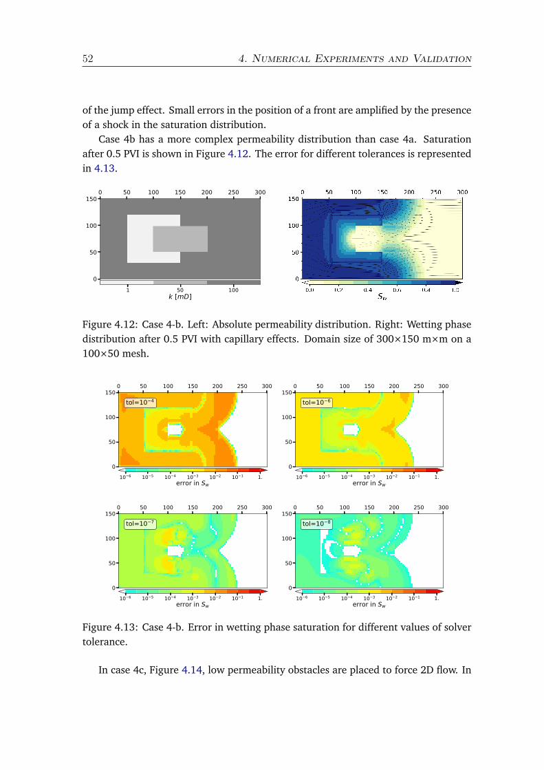
52 4. Numerical Experiments and Validation
of the jump effect. Small errors in the position of a front are amplified by the presenceof a shock in the saturation distribution.
Case 4b has a more complex permeability distribution than case 4a. Saturationafter 0.5 PVI is shown in Figure 4.12. The error for different tolerances is representedin 4.13.
0 50 100 150 200 250 300
0
50
100
150
1 50 100k [mD]
Figure 4.12: Case 4-b. Left: Absolute permeability distribution. Right: Wetting phasedistribution after 0.5 PVI with capillary effects. Domain size of 300×150 m×m on a100×50 mesh.
0 50 100 150 200 250 300
0
50
100
150tol=10 4
0 50 100 150 200 250 300
0
50
100
150tol=10 6
0 50 100 150 200 250 300
0
50
100
150tol=10 7
0 50 100 150 200 250 300
0
50
100
150tol=10 8
10 6 10 5 10 4 10 3 10 2 10 1 1.error in Sw
10 6 10 5 10 4 10 3 10 2 10 1 1.error in Sw
10 6 10 5 10 4 10 3 10 2 10 1 1.error in Sw
10 6 10 5 10 4 10 3 10 2 10 1 1.error in Sw
Figure 4.13: Case 4-b. Error in wetting phase saturation for different values of solvertolerance.
In case 4c, Figure 4.14, low permeability obstacles are placed to force 2D flow. In

4.1 Validation cases 53
the error plot, Figure 4.15, some oscillations can be observed close to the front at y =175. These oscillations in the error are associated to small variations in saturation nearjumps where saturation is close to the residual saturation. Those small variations areamplified by the logarithmic behaviour of the capillary pressure model that becomessingular for Sw = Sw,r . These oscillations have no apparent effects in the saturationor pressure distributions but can affect the convergence of the iterative solver. Thiseffect can be reduced by limiting maximum capillary pressure value or the minimumSe f f in the relative permeability model (2.31) to avoid unphysical values in capillarypressure.
0 50 100 150 200 250 300
0
50
100
150
1 50 100k [mD]
Figure 4.14: Case 4-c. Left: Absolute permeability distribution. Right: Wetting phasedistribution after 0.5 PVI with capillary effects. Domain size of 300×150 m×m on a100×50 mesh.
Impact of tolerance on the efficiency of the iterative solver is similar to the otheranalysed scenarios (see Figure 4.16). Iterative solver outperforms the direct one fortolerances above 10−8 up to a factor of 10 for tolerances above 10−5. For all theanalysed tolerances, including the highest ones, the solution is bounded an reproducethe main features of the flow. The times needed for the pressure and the saturationsolver for every case are listed in Table 4.6.
Table 4.6: Computational times and speedup for cases 4a, 4b and 4c, p correspondsto the pressure and S to the saturation solver computational time.
IMPES – Exact IMPES – tol= 10−5
time (s) p (s) S (s) time (s) p (s) S (s) #Iter speedupCase 4a 102 98 2.4 10.4 7.1 2.4 2747 9.8Case 4b 143 138 3.3 17.8 12.9 3.3 3861 8.0Case 4c 228 221 4.3 24.7 17.0 4.3 6143 9.2

54 4. Numerical Experiments and Validation
0 50 100 150 200 250 300
0
50
100
150tol=10 4
0 50 100 150 200 250 300
0
50
100
150tol=10 6
0 50 100 150 200 250 300
0
50
100
150tol=10 7
0 50 100 150 200 250 300
0
50
100
150tol=10 8
10 6 10 5 10 4 10 3 10 2 10 1 1.error in Sw
10 6 10 5 10 4 10 3 10 2 10 1 1.error in Sw
10 6 10 5 10 4 10 3 10 2 10 1 1.error in Sw
10 6 10 5 10 4 10 3 10 2 10 1 1.error in Sw
Figure 4.15: Case 4-c. Error in wetting phase saturation for different values of solvertolerance.
10 8 10 7 10 6 10 5 10 4
Solver tolerance
2
4
6
8
10
12
Rela
tive
effic
ienc
y
case 4acase 4bcase 4c
Figure 4.16: Efficiency of iterative solver in case 4 for different tolerances with ILU(0)as preconditioner.

4.1 Validation cases 55
4.1.5 Case 5. Five–spot
This case is a 2D five–spot simulation. This configuration consists on a square domainwith four wells placed in the corners of the domain and a fifth well in the middle.Flow is injected in the central well and produced in the other four or vice versa. Thisconfiguration is widely used in the oil industry because is the minimum representativeconfiguration required to simulate a matrix of injectors and producers in the secondaryoil recovery phase. In this phase gas or water is injected between producer wells todisplace the remaining reservoir oil and increase the oil production rate. When a low–viscosity fluid (air or water) displaces a high–viscosity one (oil) and both fluids areimmiscible, the interface between the two fluids is unsteady and the fluid with lowerviscosity tends to advance in narrow paths in a process called viscous fingering. Thisprocess affects drastically the efficiency of the oil displacement. This case will showthe ability of the solver to accurately reproduce the viscous fingering phenomenon.
Permeability distribution for this case has been computed with a random porousmedia generator, using several passes of random noise addition and Gaussian filter-ing. Wells are surrounded by permeable zones to avoid high unphysical pressureswhen fixed flow rate is imposed. Water is injected from the four squares of the do-main, which is initially saturated with oil. Fluid properties and relative permeabilityparameters are listed in Table 4.7. Flow is produced from a well in the centre of thedomain. Permeability distribution is shown on Figure 4.17. Injection rate is fixed foreach injector to 10−5 m2/s. The problem is solved using an uniform grid of 100×100points.
Table 4.7: Case 5 parameters.
n m Sr,1 Sr,2 kr,1 kr,2 µ1[Pa·s] µ2[Pa·s] Pc [bar]
2 2 0.1 0.1 1. 1. 10−2 10−3 0.
In previous test cases the impact of gravity and capillary pressure in the iterativesolver efficiency has been presented. In this case the impact of radial flow is analysed.In presence of punctual flow sources, pressure has a logarithmic behaviour close to theinjection point and velocities grow with the inverse of the distance to source in thiszone. A proper behaviour of the proposed method in this kind of problems is crucialfor solving efficiently the near wellbore region.
In the saturation distribution in Figure 4.17 the viscous fingering phenomena canbe seen [Sajjadi and Azaiez, 2012], fingers of less viscous phase are formed connectingthe injector wells with the producer in the middle of the domain. This phenomenais of high interest for oil industry because of the reduction in the efficiency of oil

56 4. Numerical Experiments and Validation
0 20 40 60 80 1000
20
40
60
80
100
2
1
0
1
2
3
log(mD)
0 20 40 60 80 1000
20
40
60
80
100
0.10
0.26
0.42
0.58
0.74
0.90
Sw
0 20 40 60 80 1000
20
40
60
80
100
0.10
0.26
0.42
0.58
0.74
0.90
Sw
Figure 4.17: Case 5. Top: Absolute permeability distribution. Wetting phase distribu-tion at water breakthrough for the first injector (left) and for the four injector wells(right). Domain size of 100×100 m×m with 100×100 mesh.
displacement, thus, an accurate solution of this problems is a key aspect for a reservoirsolver.
In the vicinity of wells, pressure distribution varies rapidly and small changes inthe saturation field will induce intense modifications in the pressure field in the entiredomain. In addition, fingers are unstable and error in pressure field associated withsolver tolerance and accumulated error in saturation distribution can lead to a changein the flow configuration. This effect can be noticed in Figure 4.18, for tolerancesabove 10−5 the finger flow structure is not well resolved, while for tolerances below10−6 the saturation distribution is indistinguishable from the reference solution. Theeffect of the unresolved finger structure can be observed, in the production plot inFigure 4.19, smoother fronts lead to a more effective oil displacement reflected in a

4.1 Validation cases 57
0 20 40 60 80 100[m]
0
20
40
60
80
100
[m]
exact
0 20 40 60 80 100[m]
tol=10 6
0.2
0.4
0.6
0.8
Sw
0 20 40 60 80 100[m]
0
20
40
60
80
100
[m]
tol=10 5
0 20 40 60 80 100[m]
tol=10 4
0.2
0.4
0.6
0.8
Sw
Figure 4.18: Finger structure in saturation distribution in case 5 after 1 year of in-jection for different solver tolerances. Domain size of 100×100 m×m with 100×100mesh.

58 4. Numerical Experiments and Validation
lower water cut 1 value for long simulation times.
0 100 200 300time [days]
0.0
0.2
0.4
0.6
0.8
wate
r cut
[-]
tol = 10 4
tol = 10 5
tol = 10 6
exact
10 8 10 7 10 6 10 5 10 4
Solver tolerance
4
6
8
10
12
Rela
tive
effic
ienc
y
Figure 4.19: Impact of tolerance in case 5. Left: Water cut for different tolerancevalues. Right: Iterative solver efficiency, grey dashed line show points where the flowconfiguration is wrongly predicted
In this case, efficiency is higher for low tolerances than in the other analysed cases.The radial configuration of the flow limits the time step, improving the efficiency ofthe iterative solver due to better initial guesses. The exception is the time close to thebreakthroughs, when the water front reaches the vicinity of the wells. In this regionthe pressure varies rapidly and small changes in mobilities associated to changes insaturation will induce global modifications in the pressure field. In Figure 4.19–rightthe efficiency plot is shown, and efficiencies greater than 10 have been measured,the details of the computational times are listed in Table 4.8. For tolerances greaterthan 10−5 the flow configuration changes, as have been mentioned before, and theefficiency curve is incoherent.
Table 4.8: Computational times and speedup for case 5. p corresponds to the pressureand S to the saturation solver computational time.
IMPES – Exact IMPES – tol= 10−6
time (s) p (s) S (s) time (s) p (s) S (s) #Iter speedupCase 5 4425 4281 91 393 251 91 57900 11.3
1Water cut: The ratio of water produced compared to the volume of total liquids produced

4.1 Validation cases 59
4.1.6 Case 6. SPE10 dataset 2This simulation has been performed with the 3D version of the simulator, developedfor Repsol during this thesis. Some quantitative results are shown to prove the abilityof the methodology to deal with long run simulation on industrial size problems. Thepermeability distribution of the reservoir is shown in Figure 4.20, fast variations inthe permeability field up to 8 orders of magnitude are present. In Figure 4.21 thedistribution of porosity is shown. This tricky configuration, including null porosityregions and sharp permeability variations are well resolved by the numerical algorithmshowing no oscillations or unphysical variable magnitudes.
Figure 4.20: Permeability distribution for the SPE 10 dataset 2. Cuts showing differentdomain layers.
The simulation setup consists on fives wells. One injector in the center of thedomain in which water in injected at a rate of 5000 bbl/day and four producers witha fixed pressure of 4000 psi (∼ 275.8 bar). The domain is saturated with oil withirreducible water saturation. Fluid properties are listed in Table 4.9. Rock and fluidcompressibility, as well as the dependence of the viscosity with pressure are neglectedin this simulation.
Table 4.9: Case 6 fluid properties.
n m Sr,1 Sr,2 kr,1 kr,2 µ1[Pa·s] µ2[Pa·s] g [m/s2]
2 2 0.2 0.2 1. 1. 3 · 10−3 0.3 · 10−3 0
One thousand days of injection have been simulated. The pressure distributionand the position of the water front after 35 days of simulation is shown in Figure 4.22.

60 4. Numerical Experiments and Validation
Figure 4.21: Porosity distribution for the SPE 10 dataset 2. Cuts showing differentdomain layers. The locations of the injector (red) and producers wells (blue) aremarked in the figure.
The water cut history for the four producers is plotted in Figure 4.23. No oscillationor unphysical variable magnitude have been observed. Results are in good agreementwith the published results [Christie and Blunt, 2001] despite of the simplifications inthe simulation mentioned before.
Figure 4.22: SPE10 dataset 2. Pressure distribution and water front position after 35days of simulation.

4.2 Analysis of iterative solver 61
0 200 400 600 800 1000Injection time [days]
0.0
0.2
0.4
0.6
0.8
Wat
er c
ut [-
]
Producer AProducer BProducer CProducer D
Figure 4.23: SPE10 dataset 2. Water cut history for the four producers.
4.2 Analysis of iterative solver
4.2.1 Impact of preconditioner
The success of iterative linear solvers depends highly on the preconditioner used. De-pending on the problem, some preconditioners will outperform others but there is,generally, no best one. For this solver, 3 preconditioners have been analysed. Themonitor variable of convergence is the divergence of total velocity per time step, asdefined in (3.38). This variable, used as error monitor, is almost problem independentas shown in Section 4.1.
In Figure 4.24 the convergence history for the GMRES is shown. For a fixed timestep the pressure equation has been solved using a fixed number of GMRES iterationsfor the three different preconditioners analysed. In all the cases, the pressure distri-bution from the previous time step has been used as initial guess. On the one hand,the left plot shows that from the point of view of the number of iterations, the mostexpensive the preconditioner, the fastest the convergence. On the other hand, whencomparing the total solution time, the cost of computing and applying the precon-ditioner comes into play. Now for higher tolerances, cheaper preconditioners presentlower solution times while for lower tolerances the expensive preconditioners performthe best.
It should be noticed (Figure 4.24–right) that the three methods outperform thedirect one for the case analysed, where only one order of magnitude is needed toconverge from the initial guess to get the desired divergence tolerance. This behaviouris similar in the other test cases as can be drawn from the efficiency plots for the

62 4. Numerical Experiments and Validation
0 25 50 75 100 125 150GMRES #iter
10 14
10 12
10 10
10 8
10 6
DIV
erro
r
tol=10 7
ILU(0)ILUT(4)ILUT(8)
10 3 10 2 10 1 100
GMRES time [s]10 14
10 12
10 10
10 8
10 6
DIV
erro
r
tol=10 7
ILU(0)ILUT(4)ILUT(8)exact
Figure 4.24: Convergence history for the GMRES linear solver for three different pre-conditioners. On y − axis, the error in total velocity divergence associated with theGMRES solution and on x − axis number of GMRES iteration (left) and GMRES so-lution time (right). Markers every 25 iterations. Analysis corresponds to case 3 after0.2 PVI with a tolerance of 10−7.
10 8 10 7 10 6 10 5 10 4
Solver tolerance
2
4
6
8
10
Rela
tive
effic
ienc
y
Case 2ILU0ILUT(4)ILUT(8)
10 8 10 7 10 6 10 5 10 4
Solver tolerance
2
4
6
8
10
12
Rela
tive
effic
ienc
y
Case 3ILU0ILUT(4)ILUT(8)
Figure 4.25: Efficiency of iterative solver for different preconditioners function of thedivergence tolerance.
different preconditioners shown in Figure 4.25
Both GMRES-ILUT(8) and GMRES-ILUT(4) present an approximately constant costwith respect to the Solver tolerance, as most of the computational time is spent in thecomputation of the preconditioner, i.e., the effect of the number of iterations of theGMRES is small. On the contrary, GMRES-ILU(0) presents a highly variable computa-tional cost as time is not spent in the computation of the preconditioner (it is cheap)and therefore the relative effect of the number of iterations of the GMRES is bigger

4.2 Analysis of iterative solver 63
4.2.2 GMRES restartGMRES algorithm becomes impractical when the Krylov subspace size, m, grows. Forthat reason GMRES can be restarted after m iterations using the last approximationas initial guess. This strategy accelerates the operations required during the GMRESiteration but can stagnate convergence if the system matrix is ill conditioned and notpositive definite, which is normally the case for the system arising from the pressureequation. The stagnation can be mitigated using a good preconditioner.
0 100 200 300 400#iter gmres
10 16
10 13
10 10
10 7
10 4
10 1
gmre
s erro
r
m = 20m = 50m = 100m = 150
0 100 200 300 400#iter gmres
10 16
10 13
10 10
10 7
10 4
10 1
gmre
s erro
r
m = 20m = 50m = 100m = 150
Figure 4.26: Impact of the restart iteration m in the convergence of the GMRES forcase 4a (left) and case(5) using ILU(0) preconditioner.
0 100 200 300 400#iter gmres
10 16
10 13
10 10
10 7
10 4
10 1
gmre
s erro
r
m = 20m = 50m = 100m = 150
0 100 200 300 400#iter gmres
10 16
10 13
10 10
10 7
10 4
10 1
gmre
s erro
r
m = 20m = 50m = 100m = 150
Figure 4.27: Impact of the restart iteration m in the convergence of the GMRES forcase 4a (left) and case(5) using ILUT(4) preconditioner.
Some test cases have been carried out to analyse the impact of restart in the con-vergence of GMRES. From the results shown in Figures 4.26 and 4.27, typical restart

64 4. Numerical Experiments and Validation
values below 50 can easily decelerate the convergence or even stagnate it when ILU(0)or ILUT are used, for this reason a value of 150 has been chosen for all test cases inthis work.

chapter 5
MULTIPHASE 2D IMPES SOLVER
The solver introduced in this chapter, simulates 2D, 2-phases, immiscible, non reactiveflow through porous media. The 2D code presented here, is an academic version ofthe industrial version developed for the company Repsol during this thesis. This codeis implemented for validation and optimization of the physical models, algorithmsand numerical methods used in the industrial version. In the following sections, theimplementation of the methodology described in previous chapters is detailed. Thesolver is programmed in Fortran 2008 and uses the VTK format for input/output.
The media is defined using a rock file where porosity, permeabilities and wells aredescribed. Boundary conditions, fluid properties, relative permeability as well as othersimulation parameters are supplied using a control file.
Mesh is provided within the rock file. The solver uses a rectangular cartesian gridwith uniform or variable spacing. The type of the boundary conditions is given with thesimulation kind defined in the control file. Three different configurations are available:pressure plug, flux plug and wells.
Pressure plug In this simulation pressure and saturation are imposed in the inflow(left boundary), pressure in the outflow (right boundary) and no flow condition isimposed in the top and bottom boundaries.
Flux plug In this simulation constant flow for each phase is imposed in the inflow(left boundary) and pressure in the outflow(right boundary). No flow condition isimposed in the top and bottom boundaries.
Wells In this simulation symmetry/no–flow condition is imposed in the four bound-aries. An arbitrary number of wells can be defined in the rock file. Wells are described
65

66 5. Multiphase 2D IMPES Solver
in the configuration file and can be defined as pressure wells, where pressure is fixedor flux wells, where a fixed flux for each phase is given.
5.1 Input/Output filesThe format for the input output data files is VTR due to compatibility issues. Thisformat is used natively by the visualization software Paraview and is part of the VTK(Visualization Tool Kit project). A thorough search revealed no available libraries forinput/output VTR format in Fortran and those have been developed for this thesis.
5.1.1 File formatVTR format is based on XML standard. Files are ASCII plain text and store the dataassociated to the variables as well as the grid information. The format and the librarysupport cell–centred and vertex–centered data of kinds double and single precisionfloats and integers. An example of a rock file is listed below. This file includes the griddescription (x and y distributions) and the values of the absolute permeability tensor(AbspermX and AbspermY), porosity and markers. The marker identifies the point asporous domain (marker=0) or well (marker > 0). The rock described in the examplefile is shown on Figure 5.1.
1 <?xml version ="1.0" ?>2 <VTKFile type=" RectilinearGrid " version ="0.1" format ="
ascii">3 <RectilinearGrid WholeExtent =" 1 6 1 6 1 1">4 <Piece Extent =" 1 6 1 6 1 1">5 <Coordinates >6 <DataArray type=" Float64 " Name=" x_coordinate "
NumberOfComponents ="1" format ="ascii" RangeMin ="0."RangeMax ="1.">
7 0. 0.2 0.4 0.6 0.8 1.8 </DataArray >9 <DataArray type=" Float64 " Name=" y_coordinate "
NumberOfComponents ="1" format ="ascii" RangeMin ="0."RangeMax ="1.">
10 0. 0.2 0.4 0.6 0.8 1.11 </DataArray >12 <DataArray type=" Float64 " Name=" z_coordinate "
NumberOfComponents ="1" format ="ascii" RangeMin ="0."RangeMax ="0.">
13 0.14 </DataArray >15 </ Coordinates >

5.2 Implementation methodology 67
16 <CellData >17 <DataArray type=" Float64 " Name=" abspermX "
NumberOfComponents ="1" format ="ascii" RangeMin ="1."RangeMax ="2.">
18 2. 2. 2. 2. 2. 2. 2. 2. 2.19 2. 1. 1. 1. 1. 1. 2. 2. 2.20 2. 2. 2. 2. 2. 2. 2.21 </DataArray >22 <DataArray type=" Float64 " Name=" abspermY "
NumberOfComponents ="1" format ="ascii" RangeMin ="1."RangeMax ="2.">
23 2. 2. 2. 2. 2. 2. 2. 2. 2.24 2. 1. 1. 1. 1. 1. 2. 2. 2.25 2. 2. 2. 2. 2. 2. 2.26 </DataArray >27 <DataArray type=" Float64 " Name=" porosity "
NumberOfComponents ="1" format ="ascii" RangeMin ="0.2"RangeMax ="0.2">
28 0.2 0.2 0.2 0.2 0.2 0.2 0.2 0.229 0.2 0.2 0.2 0.2 0.2 0.2 0.2 0.230 0.2 0.2 0.2 0.2 0.2 0.2 0.2 0.231 0.232 </DataArray >33 <DataArray type="Int32" Name=" marker "
NumberOfComponents ="1" format ="ascii">34 1 0 0 0 0 0 0 0 0 0 0 0 035 0 0 0 0 0 0 0 0 0 0 0 236 </DataArray >37 </CellData >38 <PointData >39 </PointData >40 </Piece >41 </ RectilinearGrid >42 </VTKFile >
Listing 5.1: Rock file example
5.2 Implementation methodology
One of the goals of the simulation code is to serve as a base for further development,for that reason, the code has been designed using a modular structure implementedwith modern object–oriented Fortran 2008. The sketch of the code is shown in Figure5.2. A brief explanation of the main blocks of the code is given below.

68 5. Multiphase 2D IMPES Solver
Figure 5.1: Rock file example visualized with Paraview.
Simulation module This is the main block, where the objects instances of theclasses described below are created.
Config class This class contains all the configuration parameters and the methodfor reading it from the parameter file.
Data class This class contains all the data structures required by the solver. Datais organised using structure–of–arrays paradigm (see Appendix A). Each variable isstored in a 2D array. The class includes a method for reading the rock file whichprovides rock data as well as the grid and problem dimensions. Point data, such aspressure or saturation; face data, like mobilities or fluxes; control data, such as timesteps or tolerances and monitoring variables are defined in this class.
IMPES solver Here, the temporal integration is implemented. Each time step, suc-cessive calls to the pressure solver, saturation solver and mobilities update are madeaccording to the IMPES algorithm.
Mobilities In this module the procedures for updating the relative permeabilitiesand computing the face mobilities are implemented, these procedures are invoked bythe IMPES solver.

5.2 Implementation methodology 69
Figure 5.2: Simplified diagram of the Darcy2D code.

70 5. Multiphase 2D IMPES Solver
Saturation solver This class contains the routines that compute face fluxes andtime step required for updating the saturation field.
Pressure solver This class includes the code for computing the system matrix de-rived form the discretisation of the pressure equation and the appropriate boundaryconditions. On each call, the matrix is assembled and the linear system is solved in-voking the linear solver.
Linear solver This class acts as a wrapper for the MKL routines for solving sparselinear systems [Intel Corporation, 2017] . A direct solver based on PARDISO [Amestoyet al., 2001] and a iterative solver based on RCI-FGMRES with several preconditioneroptions are implemented.
VTR-IO This module contains the routines needed for reading and writing files inVTR format.
Plotter In this module the routines that generate the ouput of the code are defined.Results can be produced in VTR format or directly into pdf/png or live–plot throughthe included python–matplolib wrapper.
5.2.1 Sparse matrix storageFrom the discretisation of the pressure equation (2.32), the matrix of the linear systemhas a pure penta-diagonal structure, associated to the 2D 5–point finite differencesscheme. The matrix is extremely sparse for typical sized problems, with only fivenon zero elements per row. In this scenario the use of sparse storage and algebra isrequired to be able to handle industrial scale simulations. For example, using densealgebra a matrix associated to a problem defined on a mesh of size 200× 200 wouldrequire 40000× 40000 elements× 8 Byte per elemet = 12.8 GB of RAM, only for thematrix storage. In the same case, using sparse algebra will require, for a naive noncompressed storage, 40000 × 5 elements × 8 Byte per elemet + 40000 × 2 indices ×4 Byte per index = 1.92 MB, roughly ten thousandth of the memory needed in thedense case.
There are some strategies for storing sparse matrices in a compact (compressed)form. In this code, one of the most used formats, the CSR (Compressed Sparse Row)1 isused. This format is supported by the majority of sparse linear algebra libraries (e.g.MKL [Intel Corporation, 2017], , MUMPS [Amestoy et al., 2001], PETSc [Balay et al.,2016], etc).
1This format is sometimes referred as Compressed Row Storage (CRS)

5.2 Implementation methodology 71
Compressed Sparse Storage (CSR) This format is valid for every non zero ele-ments distributions since there is no assumption about the sparsity pattern and doesnot stores any unnecessary elements.
A matrix M of size m × n and NN Z non zero values is defined using three vec-tors(A,IA,JA) where:
• A is a vector of length NN Z that contains all the non zero the values of M sortedby rows (row-major order).
• IA is of length m+1 and is defined recursively, IA(1) = 1 and IA(i) = IA(i−1)+number of non zero elements in the i − 1 row.
• JA is of length NN Z and contains the column indices of each non zero elementin the matrix M.
The values of the row i in M, stored in A, can be accessed using the vector IA inthe following way: A(IA(i) : IA(i + 1)− 1) and to the corresponding columns indices:JA(IA(i) : IA(i+1)−1), thus, vector IA is often referred as row_pointer or row_ptr. Anexample of the format is given below:
M=
1 0 0 0 02 1 1 0 00 0 1 3 00 0 0 0 4
A= (1, 2,1, 1,1, 3,4)
IA= (1, 2,5, 7,8)
JA= (1, 1,2, 3,3, 4,5)
5.2.2 ParallelisationThe implementation of the solver described in previous sections uses two differentparallelisation strategies. On the one hand loops over points or faces are parallelisedusing OpenMP as well as the maximum or minimum of an array that uses reductionsunder OpenMP. On the other hand, the linear solver uses the multithread version ofMKL–Pardiso, for the direct solver, and the multithreaded version of the FGMRES, forthe iterative one, both included in the MKL Library.

72 5. Multiphase 2D IMPES Solver
Explicit loops Most of the computational cost of the explicit saturation solver isrelated to loops over all the points or faces in the domain with no interdependencies.This kind of problems, known as embarrassingly parallel will present a high paral-lelization efficiency. To improve the efficiency of the implementation, nested loopsdue to the iteration over x and y dimensions can be collapsed to work as one biggerloop, reducing the overheads associated to the threads creation/destruction. A typicalOpenMP point–loop is listed below:
1 !$OMP PARALLEL DEFAULT ( PRIVATE ) &2 !$OMP& SHARED (a,b,c, nx , ny , dt)3 !$OMP DO COLLAPSE (2)4 do i = 1, nx5 do j = 1, ny6 a(i,j) = b(i,j)+dt*c(i,j)7 end do8 end do9 !$OMP END DO
10 !$OMP END PARALLEL
Listing 5.2: OpenMP nested loop example
Reductions Operations such as sum, min, max or average, are known as reductionoperations, taking as input an array of values an retuning a single scalar. OpenMP canlead with this kind of operations using the REDUCTION clause. The syntax used inthe code for a min and a max reduction is listed below:
1 !$OMP PARALLEL SHARED (sdot ,dt ,nx ,ny) PRIVATE (i,j)2 !$OMP DO REDUCTION (MAX: max_sdot ) REDUCTION (MIN: min_dt )3 do i = 1, nx4 do j = 1, ny5 max_sdot = max( abs( sdot(i,j) ), max_sdot )6 min_dt = min( min_dt , dt(i,j) )7 end do8 end do9 !$OMP END DO
10 !$OMP END PARALLEL
Listing 5.3: OpenMp reduction example
Linear solver The parallelisation of this part of the code relies on the multi-threadversion of MKL. Pardiso [Schenk and Gärtner, 2004], the direct solver uses a paral-lelisation at operation level (multithread vector operations) and at algorithm level,obtaining a modest efficiency with the sizes involved in the analysed cases. FGMRESuses only multithread vector operations but the algorithms are serial. Multithread

5.2 Implementation methodology 73
vector operations are only efficient when the overheads associated to the thread cre-ation/destruction are negligible compared to the cost of the serial operation whichonly occurs with huge arrays. With the sizes of the problems proposed in this work,the parallel performance of the iterative linear solver is poor.
Results of scalability are shown in Figure 5.3. As can be observed, the parallel per-formance of the mobilities computation, based on explicit loops, is nearly ideal. Thespeedup of the saturation solver which includes explicit loops, reductions an serial op-erations drops as the number of CPUs increases. In addition, loops in saturation solverare very light, with operations involving only a couple of additions or multiplications.This kind of loops are typically memory bounded, where speed is limited by memorybandwidth instead of by CPU speed, taking almost no advantage of parallelisation inshared memory architectures. This effect is studied in Appendix A.
2 4 6 8 10 12# cpu
2
4
6
8
10
12
spee
dup
totalpressuresaturationmobilities
2 4 6 8 10 12# cpu
2
4
6
8
10
12
spee
dup
totalpressuresaturationmobilities
Figure 5.3: Scalability for case 3 with tol=10−7 (left) and direct solver (right).


CONCLUSIONS
An improved methodology to simulate the multiphase immiscible flow through porousmedia in the near wellbore region has been developed.
The method is very efficient to solve problems where temporal accuracy is required.The developed numerical scheme takes advantage of the time step restriction of theIMPES method to reduce the computational cost of the implicit pressure solver byusing an iterative linear solver. Furthermore, the relation between the iterative linearsolver tolerance and the accuracy of the solution has been studied. The validity of thedeveloped strategy to improve the performance of the method without compromisingthe accuracy of the solution has been shown for complex problems including wells,gravity and capillary effects.
An improvement in computational time of up to an order of magnitude with re-spect to the conventional IMPES has been measured in a wide range of simulations.This reduction is similar to the one obtained with fully implicit methods for some con-figurations, but with higher temporal accuracy and less memory requirements. Thesefeatures can be relevant in some applications of high interest such as detailed nearwellbore simulations or transient processes.
The GMRES based solver has been tested in a wide range of scenarios to provethe robustness of the mathematical and numerical models. One of the main draw-backs when dealing with iterative solvers is the unknown efficiency and the problemdependency. Through a wide variety of tests, it has been proven that, despite showingvariable performance, the algorithm is robust and outperforms other reported strate-gies.
In addition, this thesis has been used to apply modern object–oriented Fortran toan industrial code. The methodologies, as well as modules and libraries developedare already been used in others ongoing projects.
The 2D Darcy solver presented in this work is the initial step of a new line in theresearch group in the field of multiphase flow in porous media. The solver is the basefor further development including compressibility, reactive flows and compositionalmodels.
75


Appendices
77


appendix A
DATA STRUCTURE. AOS VS SOA
One of the first decisions to make when coding a CFD algorithm is the chose of thedata structure. Usually, this kind of codes use a certain number of variables associatedwith the discretisation points and/or the discretisation faces. There are, mainly, twocriteria in these cases: defining an structure that stores all the data associated with apoint or a face and declare an array of this kind (Array of Structures, AOS), or definingan array for each variable (Structure of Arrays, SOA). Apart from the coding syntax,the main difference between these two approaches is the memory layout of the data.In the first case, all the data associated with a point is contiguous in memory andin the second case, it is the data associated to a variable the one that is contiguous.Traditionally, when programming for CPU, memory bandwidth has not been an issue,but modern processors with tens of cores and vectorization capabilities have increaseddrastically the computation performance and the memory throughput can become abottleneck. If memory bandwidth is the limiting factor, the data structure becomesdeterminant in the overall code performance.
In serial codes, memory bandwidth is not the limiting factor due to the size andhierarchy of cache memory in modern processors but, when using multi-thread par-allelisation and vectorization, the computational capability increases and thus the re-quirement of memory throughput.
For measuring the impact of the data structure in the code performance the pro-gram listed below has been used. The code consist on a variable update typicallyfound in a 2D finite differences algorithm, coded for a AOS and a SOA structures.Every single update operation has a very low arithmetical cost (only addition andmultiplications). The number of point updates per second is computed as a measureof the efficiency. The program is compiled with Intel Fortran Compiler 2017 with thefollowing optimization flags:
ifort -O3 -xavx -parallel -qopt-report=2
79

80 A. Data structure. AOS vs SOA
Tests have been carried out on a workstation with dual Intel(R) Xeon(R) CPU E5-2630@ 2.30 GHz (with Turbo Boost and Hyperthreading disabled) and 32 GB RAM DDR3@ 1333MHz.
1 include "time.f90"2
3 module types4 use iso_fortran_env , only: RP => real645 implicit none6 type soa_data7 real(kind=RP), allocatable :: a(: ,:)8 real(kind=RP), allocatable :: b(: ,:)9 real(kind=RP), allocatable :: c(: ,:)
10 real(kind=RP), allocatable :: d(: ,:)11 real(kind=RP), allocatable :: e(: ,:)12
13 end type soa_data14
15 type aos_data16 real(kind=RP) :: a17 real(kind=RP) :: b18 real(kind=RP) :: c19 real(kind=RP) :: d20 real(kind=RP) :: e21 end type aos_data22
23 end module24
25 program soavsaos26 use iso_fortran_env , only: RP => real6427 use types28 use time29 implicit none30
31 integer , parameter :: n = 500032 integer , parameter :: kmax = 2033 type ( soa_data ) :: soa34 type ( aos_data ), allocatable :: aos (: ,:)35 type (timer) :: clock36 real(kind=RP) :: t1 , t237 integer :: i,j,k38
39 allocate (soa%a(n,n))40 allocate (soa%b(n,n))41 allocate (soa%c(n,n))42 allocate (soa%d(n,n))43 allocate (soa%e(n,n))

81
44 allocate (aos(n,n))45
46 soa%a=0. _RP47 call random_number (soa%b)48 call random_number (soa%c)49 call random_number (soa%d)50 call random_number (soa%e)51
52 do j = 1, n53 do i = 1, n54 aos(i,j)%a = 0. _RP55 aos(i,j)%b = soa%b(i,j)56 aos(i,j)%c = soa%c(i,j)57 aos(i,j)%d = soa%d(i,j)58 aos(i,j)%e = soa%e(i,j)59 end do60 end do61
62 t1 = 0. _RP63 do k = 1, kmax64 call clock%start ()65 do j = 2, n-166 do i = 2, n-167 soa%a(i,j) = soa%a(i,j) + &68 soa%b(i-1,j) * soa%c(i-1,j)+ &69 soa%b(i+1,j) * soa%c(i+1,j)+ &70 soa%d(i,j -1) * soa%e(i,j -1)+ &71 soa%d(i,j+1) * soa%e(i,j+1)72 end do73 end do74 call clock%stop ()75 t1 = t1 + (clock% elapsed_time ()-t1) / kmax76 end do77
78 t2 = 0. _RP79 do k = 1, kmax80 call clock%start ()81 do j = 2, n-182 do i = 1, n-183 aos(i,j)%a = aos(i,j)%a + &84 aos(i-1,j)%b * aos(i-1,j)%c + &85 aos(i+1,j)%b * aos(i+1,j)%c + &86 aos(i,j -1)%d * aos(i,j -1)%e + &87 aos(i,j+1)%d * aos(i,j+1)%e88 end do89 end do90 call clock%stop ()

82 A. Data structure. AOS vs SOA
91 t2 = t2 + (clock% elapsed_time ()-t2) / kmax92 end do93
94 write (*,’(A,F8.3,A)’) ’SOA: ’, (n -1) *(n -1) /1 e6_RP / &95 & t1 , ’ Mpoints /s’96 write (*,’(A,F8.3,A)’) ’AOS: ’, (n -1) *(n -1) /1 e6_RP / &97 & t2 , ’ Mpoints /s’98
99
100 end program
Listing A.1: SOA vs AOS timming code
1 module time2 use iso_fortran_env , only: REAL64 , INT643 implicit none4
5 type timer6 integer (kind=INT64) , private :: crate = 07 integer (kind=INT64) , private :: cmax = 08 integer (kind=INT64) , private :: cstart = 09 integer (kind=INT64) , private :: cstop = 0
10 contains11 procedure :: start => clock_start12 procedure :: stop => clock_stop13 procedure :: elapsed14 end type timer15
16 private17 public timer18
19 contains20
21 subroutine clock_start (this)22 class(timer), intent ( inout) :: this23 call system_clock ( count_rate = this%crate)24 call system_clock ( count_max = this%cmax)25 call system_clock (count = this% cstart )26 this% cstop = 027 end subroutine28
29 subroutine clock_stop (this)30 class(timer) , intent (inout ) :: this31 integer :: t32 call system_clock (count = this%cstop)33 end subroutine34
35 function elapsed (this) result ( elapsed_time )

83
36 class(timer) , intent (inout ) :: this37 real(kind= REAL64 ) :: elapsed_time38
39 integer (kind=INT64) :: ti , tf40 ti = this% cstart41 tf = this%cstop42 if (tf == 0 ) then43 elapsed_time = -9999. _REAL6444 return45 endif46 if (tf < ti) tf = tf + this%cmax47 elapsed_time = real(tf -ti , kind= REAL64 ) /&48 & real(this%crate , kind= REAL64 )49 end function50
51 end module time
Listing A.2: time.f90
The flag -xavx tells the compiler to use, when possible, vector instructions, -parallelactivates the automatic multi-thread paralellisation and -qopt-report=2 generates acompilation report. The report indicates that the main loops at lines 65 and 81 areparallelised and vectorized automatically by the compiler.
1 2 4 6 8 10 12# procs
200
400
600
800
Mpo
ints
/s
SOAAOS
Figure A.1: Scalability of point updates per second for the two different approachesfor the multiplication loop. On y-axis, million of point updates per second.
The performance results for each strategy, AOS and SOA are plotted in Figure A.1.As can be observed, the performance of the SOA strategy outperforms by a factor of3 the AOS strategy for this kind of loops. It can be noticed as well, that the memorybandwidth becomes the computation bottleneck with more than 4 processors, this

84 A. Data structure. AOS vs SOA
fact has been checked using Intel VTune profiler that indicate that the main loops arememory bounded with more than 4 processors. In Figure A.2 the memory bandwidthfrom the profile is plotted. It is observed that the SOA strategy needs less memorywrite operations due to a better cache utilization, increasing the effective memorythroughput.
Figure A.2: Memory bandwidth utilization during test code execution Green line cor-responds to read operations and red line to write operations. Left half correspond tothe SOA loop and right half to the AOS loop. Profiled with Intel Vtune Amplifier XE2017.
Another kind of loops with high arithmetic cost per computation are also presentin the algorithm. In these loops memory bandwidth is not the limiting resource dueto a more efficient cache use. For measuring the efficiency os this kind of loops, themultiplication operation in the main loops (lines 65 and 81) is substituted by an ex-ponentiation (∼ 25 times more costly). In Figure A.3 the scalability with the expo-nentiation operation is shown. The number of updates per second is reduced due tothe extra cost of the loop operation but the scalability is near ideal for both strategiesand no signs of memory bounding are appreciated.
Based on the results shown in this chapter, the SOA strategy has been chosen be-cause of the better performance shown in both light and heavy arithmetic loops.

85
1 2 4 6 8 10 12# procs
50
100
150
200
250
Mpo
ints
/s
SOAAOS
Figure A.3: Scalability of point updates per second for the two different approachesfor the exponentiation loop.


appendix B
FORTRAN – PYTHON PLOTTING
Fortran lacks of native utilities for graphical data representation. For this purpose,python and Matplotlib [Hunter, 2007] have been used. Matplotlib is a flexible, highlyconfigurable python library that produces high quality figures for publication in mul-tiple formats as well as configurable and interactive screen plots.
Data for plotting is written by Fortran code using stream unformatted files, in-cluded in the Fortran 2003 standard. Stream files do not include any records termi-nation (which, depending on the platform, may be line–feeds, or carriage–returns, orboth). These files can be read easily from python using numpy [van der Walt et al.,2011]. A minimal working example for writing–reading–plotting is shown below. InCode B.1 the Fortran side of the interface is listed. The python side of the code isshown in Code B.2.
1 program write_stream2 implicit none3 integer , parameter :: nx = 21, ny = 114 integer :: i, outfile5 real(kind =8) :: x(nx), y(ny), p(nx -1,ny -1)6
7 x(1: nx) = [(1 d0*i, i = 0,nx -1)]8 y(1: ny) = [(1 d0*i, i = 0,ny -1)]9 call random_number (p)
10
11 open ( newunit =outfile ,file=’data.dat ’, &12 & form=" unformatted ",access =" stream ")13 write ( outfile ) nx , ny , x, y, p14 close ( outfile )15 end program
Code B.1: Minimal working example of stream writting in fortran.
87
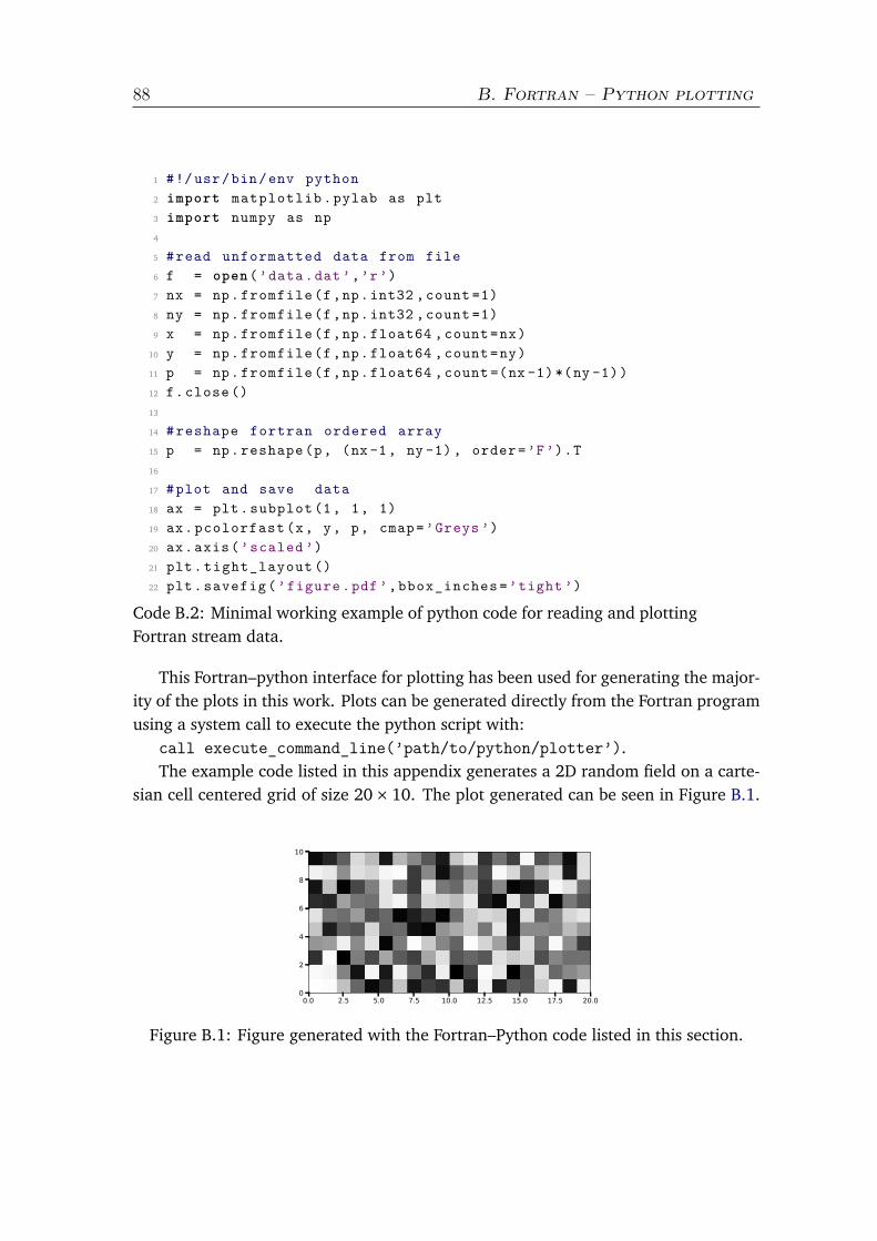
88 B. Fortran – Python plotting
1 #!/ usr/bin/env python2 import matplotlib .pylab as plt3 import numpy as np4
5 #read unformatted data from file6 f = open(’data.dat ’,’r’)7 nx = np. fromfile (f,np.int32 ,count =1)8 ny = np. fromfile (f,np.int32 ,count =1)9 x = np. fromfile (f,np.float64 ,count=nx)
10 y = np. fromfile (f,np.float64 ,count=ny)11 p = np. fromfile (f,np.float64 ,count =(nx -1) *(ny -1))12 f.close ()13
14 # reshape fortran ordered array15 p = np. reshape (p, (nx -1, ny -1) , order=’F’).T16
17 #plot and save data18 ax = plt. subplot (1, 1, 1)19 ax. pcolorfast (x, y, p, cmap=’Greys ’)20 ax.axis(’scaled ’)21 plt. tight_layout ()22 plt. savefig (’figure .pdf ’,bbox_inches =’tight ’)
Code B.2: Minimal working example of python code for reading and plottingFortran stream data.
This Fortran–python interface for plotting has been used for generating the major-ity of the plots in this work. Plots can be generated directly from the Fortran programusing a system call to execute the python script with:
call execute_command_line(’path/to/python/plotter’).The example code listed in this appendix generates a 2D random field on a carte-
sian cell centered grid of size 20× 10. The plot generated can be seen in Figure B.1.
0.0 2.5 5.0 7.5 10.0 12.5 15.0 17.5 20.00
2
4
6
8
10
Figure B.1: Figure generated with the Fortran–Python code listed in this section.

BIBLIOGRAPHY
[Aarnes et al., 2007] Aarnes, J. E., Gimse, T., and Lie, K.-A. (2007). An introductionto the numerics of flow in porous media using Matlab, pages 265–306. SpringerBerlin Heidelberg, Berlin, Heidelberg.
[Amarnath, 1999] Amarnath, A. (1999). Enhanced Oil Recovery Scoping Study. Elec-tric Power Research Institute (EPRI).
[Amestoy et al., 2001] Amestoy, P. R., Duff, I. S., Koster, J., and L’Excellent, J.-Y.(2001). A fully asynchronous multifrontal solver using distributed dynamicscheduling. SIAM Journal on Matrix Analysis and Applications, 23(1):15–41.
[Balay et al., 2016] Balay, S., Abhyankar, S., Adams, M. F., Brown, J., Brune, P.,Buschelman, K., Dalcin, L., Eijkhout, V., Gropp, W. D., Kaushik, D., Knepley,M. G., McInnes, L. C., Rupp, K., Smith, B. F., Zampini, S., Zhang, H., and Zhang,H. (2016). Petsc web page. http://www.mcs.anl.gov/petsc.
[Barrett et al., 1994] Barrett, R., Berry, M., Chan, T. F., Demmel, J., Donato, J., Don-garra, J., Eijkhout, V., Pozo, R., Romine, C., and der Vorst, H. V. (1994). Templatesfor the solution of linear systems: building blocks for iterative methods, 2nd edition.SIAM, Philadelphia, PA.
[Bear, 1972] Bear, J. (1972). Dynamics of fluids in porous media. Dover Civil andMechanical Engineering Series. Dover.
[Bear and Bachmat, 1990] Bear, J. and Bachmat, Y. (1990). Introduction to modelingof transport phenomena in porous media. Theory and Applications of Transportin Porous Media. Springer Netherlands, 1 edition.
[Boek and Venturoli, 2010] Boek, E. S. and Venturoli, M. (2010). Lattice-boltzmannstudies of fluid flow in porous media with realistic rock geometries. Computers& Mathematics with Applications, 59(7):2305–2314.
89

90 BIBLIOGRAPHY
[Bowers and Katsube, 2002] Bowers, G. and Katsube, T. (2002). The role of shalepore structure on the sensitivity of wire-line logs to overpressure. AAPG Memor,76:43–60.
[Brekke et al., 1993] Brekke, K., Johansen, T., and Olufsen, R. (1993). A new mod-ular approach to comprehensive simulation of horizontal wells. In SPE AnnualTechnical Conference and Exhibition, Houston, Texas. Society of Petroleum Engi-neers.
[Brooks and Corey, 1964] Brooks, R. and Corey, A. (1964). Hydraulic properties ofporous media. Colorado State University Hydrology Papers. Colorado State Uni-versity.
[Brown and Walker, 1997] Brown, P. N. and Walker, H. F. (1997). GMRES on (nearly)singular systems. SIAM J. Matrix Anal. Appl., 18(1):37–51.
[Buckley and Leverett, 1942] Buckley, S. E. and Leverett, M. C. (1942). Mechanismof fluid displacement in sands. Trans, AIME, 146(1):107–116.
[Cense and Berg, 2009] Cense, A. W. and Berg, S. (2009). The vicous-capillary para-dos in 2-phase flow in porous media. In International Symposium of the Societyof Core Analysts.
[Chen, 2001] Chen, Z. (2001). Degenerate two-phase incompressible flow. Journalof Differential Equations, 171(2):203 – 232.
[Chen et al., 2004] Chen, Z., Huan, G., and Li, B. (2004). An improved im-pes method for two-phase flow in porous media. Transport in Porous Media,54(3):361–376.
[Christie and Blunt, 2001] Christie, M. and Blunt, M. (2001). Tenth spe compara-tive solution project: a comparison of upscaling techniques. In SPE ReservoirSimulation Symposium. Society of Petroleum Engineers.
[Coats, 2003] Coats, K. (2003). IMPES stability: the CFL limit. SPE Journal,8(03):291–297.
[Coats et al., 1969] Coats, K. H., of Texas., U., of Engineering., C., and Institutes., E.(1969). Elements of reservoir simulation. University of Texas, [Austin, TX].
[Collins and Nghiem, 1992] Collins, D. and Nghiem, L. (1992). An efficient ap-proach to adaptive-implicit compositional simulation with an equation of state.SPE Reservoir Engineering, 7(May):259–264.

BIBLIOGRAPHY 91
[da Silva et al., 2016] da Silva, R. S., Lyra, P. R. M., Willmersdorf, R. B., and de Car-valho, D. K. E. (2016). A higher resolution edge-based finite volume method forthe simulation of the oil-water displacement in heterogeneous and anisotropicporous media using a modified IMPES method. International Journal for Numer-ical Methods in Fluids, 82(12):953–978.
[Dawson et al., 1997] Dawson, C. N., Klie, H., Wheeler, M. F., and Woodward, C. S.(1997). A parallel , implicit , cell-centered method for two-phase flow with a pre-conditioned Newton–Krylov solver. Computational Geosciences, 1(1997):215–249.
[Ding, 2011] Ding, D. (2011). Coupled simulation of near-wellbore and reservoirmodels. Journal of Petroleum Science and Engineering, 76(1-2):21–36.
[Dumkwu et al., 2012] Dumkwu, F. A., Islam, A. W., and Carlson, E. S. (2012).Review of well models and assessment of their impacts on numerical reser-voir simulation performance. Journal of Petroleum Science and Engineering, 82-83:174–186.
[Ewing, 1983] Ewing, R. (1983). 1. problems arising in the modeling of processes forhydrocarbon recovery. In Frontiers in Applied Mathematics, pages 3–34–. Societyfor Industrial and Applied Mathematics.
[Franc et al., 2016] Franc, J., Horgue, P., Guibert, R., and Debenest, G. (2016).Benchmark of different CFL conditions for IMPES. Comptes Rendus Mécanique,344(10):715 – 724.
[Hornung and Jäger, 1991] Hornung, U. and Jäger, W. (1991). Diffusion, convec-tion, adsorption, and reaction of chemicals in porous media. Journal of Differ-ential Equations, 92(2):199 – 225.
[Hoteit and Firoozabadi, 2008] Hoteit, H. and Firoozabadi, A. (2008). Numericalmodeling of two-phase flow in heterogeneous permeable media with differentcapillarity pressures. Advances in Water Resources, 31(1):56–73.
[Hunter, 2007] Hunter, J. D. (2007). Matplotlib: A 2d graphics environment. Com-puting In Science & Engineering, 9(3):90–95.
[Hurtado et al., 2006] Hurtado, F., Maliska, C., and Silva, A. (2006). A variabletimestep strategy for accelerating the IMPES solution algorithm in reservoir sim-ulation. Proceedings of the XXVII Iberian Latin American Congress on Computa-tional Methods in Engineering. Belém, Brasil: UFPA, (September):14.

92 BIBLIOGRAPHY
[Intel Corporation, 2017] Intel Corporation (2017). Developer reference for Intel®Math Kernel Library - Fortran.
[Karlo et al., 2009] Karlo, D., Carvalho, E. D., Soares, R., Roberto, P., and Lyra, M.(2009). A 3-d edge-based higher order finite volume procedure for the simula-tion of two phase flow of oil and water in porous media using a modified impes.Proceedings of COBEM 2009.
[Kou and Sun, 2010a] Kou, J. and Sun, S. (2010a). A new treatment of capillarity toimprove the stability of impes two-phase flow formulation. Computers & Fluids,39(10):1923 – 1931.
[Kou and Sun, 2010b] Kou, J. and Sun, S. (2010b). On iterative IMPES formulationfor two phase flow with capillarity in heterogeneous porous media. InternationalJournal of Numerical Analysis and . . . , 1(1):20–40.
[Kuzmin, 2006] Kuzmin, D. (2006). On the design of general-purpose flux limitersfor finite element schemes. i. scalar convection. Journal of Computational Physics,219(2):513 – 531.
[Künze et al., 2013] Künze, R., Lunati, I., and Lee, S. H. (2013). A multilevel multi-scale finite-volume method. Journal of Computational Physics, 255:502–520.
[Lee et al., 2011] Lee, T., Leok, M., and McClamroch, N. H. (2011). Geometric nu-merical integration for complex dynamics of tethered spacecraft. Proceedings ofthe 2011 American Control Conference, (March):1885–1891.
[Leeftink et al., 2015] Leeftink, T., Latooij, C., and Rossen, W. (2015). Injectivityerrors in simulation of foam eor. Journal of Petroleum Science and Engineering,126:26–34.
[Leverett, 1941] Leverett (1941). Capillary behavior in porous solids. Trans, AIME,(142):159–172.
[Liu et al., 2016] Liu, H., Wang, K., Chen, Z., Luo, J., Deng, H., and He, Y. (2016).Numerical simulation of multi-phase flow in porous media on parallel comput-ers.
[Mcdowell et al., 2016] Mcdowell, A., Zarrouk, S. J., and Clarke, R. (2016). Mod-elling viscous fingering during reinjection in geothermal reservoirs. Geothermics,64:220–234.

BIBLIOGRAPHY 93
[Muccino et al., 1998] Muccino, J. C., Gray, W. G., and Ferrand, L. A. (1998). Towardan improved understanding of multiphase flow in porous media. Reviews ofGeophysics, 36(3):401–422.
[Nessyahu and Tadmor, 1990] Nessyahu, H. and Tadmor, E. (1990). Non-oscillatorycentral differencing for hyperbolic conservation laws. Journal of ComputationalPhysics, 87(2):408 – 463.
[Oberkampf and Roy, 2010] Oberkampf, W. L. and Roy, C. J. (2010). Verificationand validation in scientific computing. Cambridge University Press, New York,NY, USA, 1st edition.
[Panfilov et al., 2012] Panfilov, M., Ghesmoune, M., and Abadpour, A. (2012).Method of negative saturation and interface stabilization for multiphase com-positional flow in porous media. In ECMOR XIII - 13th European Conference onthe Mathematics of Oil Recovery.
[Pavone, 1992] Pavone, D. (1992). Observations and correlations for immiscibleviscous-fingering experiments. SPE Reservoir Engineering, 7(2):187–194.
[Peaceman, 1978] Peaceman, D. (1978). Interpretation of well-block pressuresin numerical reservoir simulation. Society of Petroleum Engineers Journal,18(3):183–194.
[Pourafshary et al., 2009] Pourafshary, P., Varavei, A., Sepehrnoori, K., and Podio,A. (2009). A compositional wellbore/reservoir simulator to model multiphaseflow and temperature distribution. Journal of Petroleum Science and Engineering,69(1-2):40–52.
[Riaz and Meiburg, 2003] Riaz, A. and Meiburg, E. (2003). Three-dimensional mis-cible displacement simulations in homogeneous porous media with gravity over-ride. Journal of Fluid Mechanics, 494:95–117.
[Saad, 2003] Saad, Y. (2003). Iterative Methods for Sparse Linear Systems: SecondEdition. Society for Industrial and Applied Mathematics.
[Saad and Schultz, 1986] Saad, Y. and Schultz, M. H. (1986). GMRES: A generalizedminimal residual algorithm for solving nonsymmetric linear systems. SIAM J. Sci.Stat. Comput., 7(3):856–869.
[Sajjadi and Azaiez, 2012] Sajjadi, M. and Azaiez, J. (2012). Thermo-viscous fin-gering in heterogeneous media. In SPE Heavy Oil Conference Canada. Society ofPetroleum Engineers.

94 BIBLIOGRAPHY
[Schenk and Gärtner, 2004] Schenk, O. and Gärtner, K. (2004). Solving unsymmet-ric sparse systems of linear equations with pardiso. Future Generation ComputerSystems, 20(3):475 – 487. Selected numerical algorithms.
[Sheldon et al., 1959] Sheldon, J. W., Zondeck, B., and Cardwell, W. J. (1959). Onedimensional, incompressible, noncapillary two-phase fluid flow in porous media.Trans, AIME, 216:290–296.
[Shi et al., 2015] Shi, J., Huang, L., Li, X., and Sepehrnoori, K. (2015). Productionforecasting of gas condensate well considering fluid phase behavior in the reser-voir and wellbore. Journal of Natural Gas Science and Engineering, 24:279–290.
[Simmons, 2008] Simmons, C. T. (2008). Henry darcy (1803–1858): Immortalisedby his scientific legacy. Hydrogeology Journal, 16(6).
[Stone and Garder Jr., 1961] Stone, H. L. and Garder Jr., A. O. (1961). Analysis ofgas-cap or dissolved-gas drive reservoirs. T. SPE AIME, 1(2).
[Sun et al., 2009] Sun, P., Xue, G., Wang, C., and Xu, J. (2009). Fast numerical simu-lation of two-phase transport model in the cathode of a polymer electrolyte fuelcell. Commun. Comput. Phys., 6(1):49–71.
[Sweby, 1984] Sweby, P. K. (1984). High resolution schemes using flux limiters forhyperbolic conservation laws. SIAM Journal on Numerical Analysis, 21(5):995–1011.
[Tan and Kalogerakis, 1991] Tan, T. B. and Kalogerakis, N. (1991). A fully implicit,three-dimensional, three-phase simulator with automatic history-matching ca-pability. Proc. of the 11TH SPE Reservoir Simulation Symp. (Anaheim, California),pages 35–46.
[Todd et al., 1972] Todd, M., O’Dell, P., and Hirasaki, G. (1972). Methods for in-creased accuracy in numerical reservoir simulators. Society of Petroleum Engi-neers Journal, 12(6):515–530.
[van der Walt et al., 2011] van der Walt, S., Colbert, S. C., and Varoquaux, G.(2011). The NumPy array: A structure for efficient numerical computation.Computing in Science Engineering, 13(2):22–30.
[Van Genuchten, 1980] Van Genuchten, M. T. (1980). A closed-form equation forpredicting the hydraulic conductivity of unsaturated soils. Soil science society ofAmerica journal, 44(5):892–898.

BIBLIOGRAPHY 95
[Webb, 2006] Webb, S. W. (2006). Gas transport mechanisms, chapter 2, pages 5–26.Springer Netherlands, Dordrecht.
[Whitaker, 1986] Whitaker, S. (1986). Flow in porous media i: A theoretical deriva-tion of Darcy’s law. Transport in Porous Media, 1(1):3–25.
[Wu and Qin, 2009] Wu, Y.-s. and Qin, G. (2009). A generalized numerical approachfor modeling multiphase flow and transport in fractured porous media. Commu-nications in Computational Physics, 6(1):85–108.
[Yang et al., 2016] Yang, H., Yang, C., and Sun, S. (2016). Active-set reduced-spacemethods with nonlinear elimination for two-phase flow problems in porous me-dia. SIAM Journal on Scientific Computing, 38(4):B593–B618.
[Zeng and Grigg, 2006] Zeng, Z. and Grigg, R. (2006). A criterion for non-Darcyflow in porous media. Transport in Porous Media, 63(1):57–69.