9 SCIENTIFIC HIGHLIGHT OF THE MONTH: ”Core-Level

Shifts in Complex Metallic Systems from First Principles”

Core-Level Shifts in Complex Metallic Systems fromFirst Principles

W. Olovsson

Department of Materials Science and Engineering, Kyoto University, Sakyo, Kyoto 606-8501,

Japan

C. Goransson, T. Marten, and I.A. Abrikosov

Department of Physics, Chemistry and Biology, Linkoping University, SE-581 83 Linkoping,

Sweden

Abstract

We show that core-level binding energy shifts (CLS) can be reliably calculated within

Density-functional theory. The scheme includes both the initial (electron energy eigenvalue)

as well as final state (relaxation due to core-hole screening) effects in the same framework.

The results include CLS as a function of composition in substitutional random bulk and

surface alloys. Sensitivity of the CLS to the local chemical environment in the bulk and

at the surface is demonstrated. A possibility to use the CLS for structural determination

is discussed. Finally, an extension of the model is made for Auger kinetic energy shift

calculations.

1 Introduction

Electrons that occupy the orbitals closer to the atomic nucleus are tightly bound. These have

experimentally well resolved binding energies, and are often referred to as core-electrons. The

binding energy EB of a core-electron in an atom is typically sensitive to the atoms specific

chemical environment. This fact can be used to gain a deeper understanding of the underlying

physical properties related to the electronic structure and bonding in the systems under study.

One very useful aspect is that due to its sensitivity to the chemical environment, EB can be

used as a tool for structural determination. Another interesting aspect is that while the binding

energy of a core-level i in a substitutional random alloy can be studied as a function of the

global composition of the alloy, the specific local environment around each and every atom at

a particular composition will lead to some differences in EB, leading to the effect of disorder

broadening of the core spectral lines.

It is a common practice to analyze core-level binding energies in terms of a difference, a core-

level binding energy shift (CLS), against some reference energy E refB , which in principle can be

66

chosen arbitrarily,

EexpCLS = EB −Eref

B . (1)

In the case of solids the reference is most often the corresponding core-level binding energy

in the pure bulk metal. In experiments the sign of the shift is determined from a convention

that the binding energies of the core electrons are positive, EB > 0. Thus, if ECLS < 0 the

electrons are less tightly bound compared to the reference system. Also note that shifts are

especially helpful in comparison with theory, due to that differences in energy are typically more

trustworthy than directly calculated ionization energies, as errors may cancel. CLSs have been

shown to be related to various material properties, such as the cohesive energy [1], the heat of

mixing [2, 3], segregation energy [4] and charge transfer [5, 6, 7]. Over the years, different kinds

of binding energy shifts have been studied, including the CLS between free atoms and atoms

in a metal, as well as CLS between atoms at the surface and in the bulk , the so-called surface

core-level shift (SCLS). Shifts are also obtained for molecules, where they can be significantly

larger than in solids.

Experimentally it is relatively easy to measure binding energies using x-ray photoelectron spec-

troscopy (XPS). In XPS the input is a monochromatic (fixed energy) beam of photons with an

energy ~ω > 1000 eV, directed towards the surface of a sample. The output is in the form of

photoionized electrons whose kinetic energies EKIN are measured, and the result is collected in

an energy distribution curve, or spectra, showing the intensity of the photoemitted electrons vs

their binding energies, defined by

EB = ~ω −EKIN − φ. (2)

In Eq.(2) φ is the work function, the lowest energy an electron must overcome to escape from

the surface to the vacuum level, Evac. In the case of atoms and molecules the binding energy

zero is set to Evac, but for solids the Fermi level, EF , is typically used as the zero.

A way to model the electron photoemission process is to divide it into two separate steps, first

an unperturbed initial state before the excitation of a core-electron at the core-level i, and

secondly a final state describing the system, but now with a core-hole in i:th level. While the

orbital energy εi can be readily calculated for a core-electron in the unperturbed system, the

experimentally measured binding energy depends in general on the relaxation effects, both in the

core-region and for the valence charge, because of the core-hole present in the final state. The

observed binding energy is better described as a many-body effect, rather than as a one electron

property. Consequently, one can think of possible complications in theoretical calculations of

the CLS within DFT.

There are a number of effects which contribute to the CLS. Following Weinert and Watson [8]

one must for instance consider: interatomic charge transfer, changes in the screening of the final

state of the core-hole, changes in the Fermi-level relative to the center of gravity of bands, intra-

atomic charge transfer, and redistribution of charge due to bonding and hybridization. This

implies that a universally accurate model needs to take all these contributions into account. It

is also important to point out that if an experimental shift is near zero, this does not necessarily

67

mean that the environment for the examined and reference atoms are the same. On the contrary

it must be taken into account that different effects mentioned above may cancel each other. For

more information on experimental technique and binding energy shifts, see for instance the book

by Hufner [9], and a review by Egelhoff [10].

The theoretical models for the calculations of the core-level binding energy shifts within density

functional theory (DFT) can be classified in three major groups, based on the complete screening

picture, the transition state model and the initial state approximation, respectively. We will

focus on the complete screening picture, used in most of our calculations and analysis. Observe

that the complete screening picture and the transition state model both include initial and final

state effects, though total energies of systems are used in the complete screening scheme and

energy eigenvalues in the transition state model. Results from the transition state model have

been compared with those from complete screening calculations, while initial state shifts (−∆ε i)

have been used mostly to illuminate the final state effects. Also notice that in principle it is the

shift that is considered in the theoretical models, the calculational methods are generally more

accurate for differences in energies, as mentioned above. The overall shape of the spectra from

many-body interactions is not considered here. The continued development of photoelectron

spectroscopy towards increased resolution encourages a direct comparison between experiment

and theory.

All calculations were performed within the density functional theory [11, 12]. In most cases the

Green’s function technique in the atomic sphere approximation, combined with the computa-

tionally efficient coherent potential approximation (CPA), was used [13, 14, 15]. To study local

environment effects on the disorder broadening of the spectral core-lines, supercell calculations

were done using the locally self-consistent Green’s function method, LSGF [16, 17], and the

Vienna ab initio simulation package, VASP [18, 19, 20, 21]. For further details the reader is

refered to the above papers concerning the methods and the specific papers with the results in

Refs. [22, 23, 24, 28, 29, 30, 31, 32, 33, 34].

The paper is organized as follows, a background of the complete screening picture and the

transition state model is introduced in Sec. 2 and 3, respectively. A comparison between different

theoretical models is presented in Sec. 4. Sec. 5 discusses CLSs as a function of the global

composition in disordered alloys. In Sec. 6 the disorder broadening of the spectral core-lines is

investigated in connection with the local environment effects in random substitutional alloys.

The CLS for atoms at interfaces are compared with disordered bulk systems in Sec. 7. Examples

of the application of SCLS for structural determination are given in Sec. 8, and an extension of

the complete screening picture for the calculations of Auger kinetic energy shifts is presented in

Sec 9.

2 Complete screening picture

In the complete screening picture for calculating the binding energy shift in Eq. (1), only total

energies, or thermodynamic properties, are needed. In more details the CLS is obtained from

considering the total energies of a system, first in its unperturbed initial state, and second in its

relaxed final state with a core-hole at a single core-ionized atom. The most important assumption

68

here is that the final state is fully relaxed in the sense that the core-hole is completely screened

by the valence electrons in metallic systems. The initial and final states of the core-ionization

can be connected through a Born-Haber cycle in a thermodynamical model approach. The core-

ionized atom Z∗ (atomic number Z) is replaced by the next element in the periodic table, Z+1,

hence the method is often refered to as the (Z+1)- or equivalent core approximation. The core-

hole is assumed to effectively act as an extra proton in the atom, such that the screening by the

valence charge of Z∗ is essentially the same as the valence charge in the Z+1 atom. Born-Haber

cycles provide a more intuitive perspective to the calculation and makes it possible to obtain

CLSs and thermodynamical properties from other experimental measurements. In particular,

the complete screening picture in connection with the Born-Haber cycle was used by Johansson

and Martensson [1] to calculate the CLS between a free atom and an atom in a metal.

However, it is also possible to calculate the complete screening picture CLS from first principles,

taking into account the internal relaxation of the core-electrons (e.g. without the equivalent

core approximation) as well as the total screening by the valence electrons, according to

EcsCLS = µi − µref

i . (3)

The shift is here given by the difference in generalized thermodynamic chemical potentials, ∆µ i,

for the ionization of a specific core-level i at atom A in a system of interest (e.g. a random

binary alloy A1−xBx) related to the ionization energy in a reference system (e.g. pure bulk

metal A). Notice the correspondence to the experimental sign convention in Eq. (1). The first

principles approach has been employed before, for instance to calculate surface core-level shifts

(SCLS) [35, 36]. One other advantage of Eq. (3), in view of our particular implementation is

that it is a proper way to calculate chemical potentials using the CPA formalism [37].

In Fig. 1 an atom A is shown in its (a) initial state, and (b) final state A∗ after the ejection of

a core-electron from state i. The resulting core-hole is assumed to be completely screened, as

indicated by the extra charge in the local valence band DOS at the atom, effectively correspond-

ing to one extra electron in the valence band. This is modeled in the calculations by promotion

of an electron to the lowest unoccupied valence state, preserving the charge-neutrality of the

system. The core-levels i, j and k will also shift their positions due to the presence of a core-hole

in the atom, Fig 1 (b). We would like to point out that within a psedupotential approach the

equivalent core approximation can still be used, and it gives results in good agreement with

calculations which do not use the Z + 1 approximation.

In Fig. 2 a comparison is made between the valence band DOS of core-ionized Cu atoms, Cu∗,

to the valence state of Zn atoms used to model Cu∗ within the (Z+1)-approximation. For the

VASP calculations in Ref. [34] the (Z+1)-approximation was used. An alternative route in VASP

is to create a specific potential for the core-ionized atom [38].

Here we recall that as a first approximation to CLS in metallic systems one often uses the

difference in core-electron energy eigenvalues, which are readily available as side product in

conventional computations. All energy eigenvalues ε below are calculated with respect to the

Fermi-level, and the co-called initial state CLS is defined as

69

Figure 1: (a) Initial and (b) final states of the photoemission process. An ejection of the core-

electron from level i results in a core-hole at this level. The effect of screening is shown by the

increased occupation of the local valence band DOS in (b) compared to (a).

EisCLS = −εi + εref

i . (4)

In EisCLS all final state effects are neglected, and it should therefore be used with some caution,

especially considering that the eigenenergies of the Kohn-Sham orbitals strictly speaking don’t

have any physical meaning, and correspond to an auxiliary system of quasiparticles designed to

produce the ground state charge density of a true many-body system.

3 Transition state model

The transition state model is based on an extension to DFT made by Janak [39], introducing

the occupation numbers ηi (0 ≤ ηi ≤ 1) for the Kohn-Sham orbitals in the expression for the

charge density,

n(r) =∑

i

ηi|ψi(r)|2. (5)

Now the Kohn-Sham equation can formally be solved self-consistently for a non-integral elec-

tron occupation. The introduction of the occupation numbers yields a modified total energy

functional E. In general E 6= E, but if ηi have the form of the Fermi-Dirac distribution, E is

numerically equal to E. Janak’s theorem states that

∂E

∂ηi= εi, (6)

independent on the exchange-correlation functional. It follows from the equation that when η i

have the form of a Fermi-Dirac distribution, E is minimized at the end-points (ηi is equal to 1

or 0) and then it is equal to the ground-state energy of the system.

70

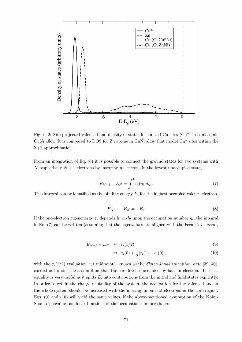
Figure 2: Site-projected valence band density of states for ionized Cu sites (Cu∗) in equiatomic

CuNi alloy. It is compared to DOS for Zn atoms in CuNi alloy that model Cu∗ sites within the

Z+1 approximation.

From an integration of Eq. (6) it is possible to connect the ground states for two systems with

N respectively N + 1 electrons by inserting η electrons in the lowest unoccupied state,

EN+1 −EN =

∫ 1

0

εi(ηi)dηi. (7)

This integral can be identified as the binding energy Ei for the highest occupied valence electron,

EN+1 −EN = −Ei. (8)

If the one-electron eigenenergy εi depends linearly upon the occupation number ηi, the integral

in Eq. (7) can be written (assuming that the eigenvalues are aligned with the Fermi-level zero),

EN+1 −EN ≈ εi(1/2) (9)

≈ εi(0) +1

2[εi(1) − εi(0)], (10)

with the εi(1/2) evaluation “at midpoint”, known as the Slater-Janak transition state [39, 40],

carried out under the assumption that the core-level is occupied by half an electron. The last

equality is very useful as it splits Ei into contributions from the initial and final states explicitly.

In order to retain the charge neutrality of the system, the occupation for the valence band in

the whole system should be increased with the missing amount of electrons in the core-region.

Eqs. (9) and (10) will yield the same values, if the above-mentioned assumption of the Kohn-

Sham eigenvalues as linear functions of the occupation numbers is true.

71

The evaluation at midpoint was used to calculate CLSs according to the transition state model

in Ref. [29],

EtsCLS = −εi(1/2) + εref

i (1/2), (11)

with fewer calculations needed compared to the last scheme in Eq. (9). Notice the similarity to

the initial state shift in Eq. (4). The difference is that the energy eigenvalues here are obtained

from core-levels with half an electron promoted to the valence band, and that the corresponding

sites are considered as impurities in systems with conventional occupation at core levels at all

other atoms. It was shown [29] that the results for the transition state model, Eq. (9), compare

well with the complete screening picture, which will also be illustrated in the next section.

One can also use Eq.(10) when calculating the CLSs, which will yield the equation

EtsCLS =

1

2

[

− εi(0) + εrefi (0)

]

+1

2

[

− εi(1) + εrefi (1)

]

. (12)

Since Eqs. (11) and (12) will only yield the same result if the Kohn-Sham eigenvalues are linear

functions of their corresponding occupation numbers, comparing these two equations provides

us with a way to evaluate the assumption of the linear dependence of εi on ηi.

Apart from the transition state CLS calculations, we have (see Ref. [33]) performed calculations

on different core-levels in several alloy systems in order to verify the above-mentioned assumption

of linearity. For each core-level and system the Kohn-Sham eigenvalues have been calculated for

η = 0.0, 0.1, . . . , 0.9, 1.0. The results have then been used for linear interpolations, where the

norm of residuals have been calculated. This means 11 different self-consistent calculations have

been done for each core-level and system.

The Kohn-Sham eigenvalues for Cu 2p3/2 and Pt 4f7/2 in Cu50Pt50 as functions of their occu-

pation numbers are shown in Fig. 3. For the sake of brevity, we present only one alloy system;

more calculations can be found in Ref. [33]. Though the graph indicate a linear relationship

between ε(η) and η, the norm of residuals is 0.07 Ry for Cu and 0.02 Ry for Pt.

However, since the energy level is much higher for Cu 2p3/2, this does not mean that the de-

pendence of the eigenvalue for this electronic state on the occupation number is less linear than

that for Pt 4f7/2. It is shown in Ref. [33] that the deeper in the core the electronic state is, the

more linear the corresponding Kohn-Sham eigenvalue.

As reference for the CLS we have also used these results to numerically evaluate the integral in

Eq. (7) by using all 11 points or by using 3 points (i.e. η = 0, 1/2, 1). A comparison of different

schemes for the calculations of hte CLS is given in the next section.

4 Comparison of different theoretical models

In order to compare different schemes for the calculation of the CLS, we present in Fig. 4

the results obtained for the CuPt fcc alloy as function of the Pt concentration. Here upwards

triangles denote transition state CLS obtained from Eq. (11) [”TS(1,0)”] and downward triangles

72

0 0.2 0.4 0.6 0.8 1

67

68

69

70

71

0 0.2 0.4 0.6 0.8 1Occupation

4.8

5

5.2

5.4

5.6K

ohn-

Sham

eig

enva

lue

(Ry)

Cu 2p3/2

Pt 4f7/2

Figure 3: Kohn-Sham eigenvalues in Cu50Pt50 as functions of the occupation number.

denote transition state CLS from Eq. (12) [”TS(1/2)”], squares denote the initial state (IS) shifts,

diamonds complete screening (CS) shifts, circles transition state calculations with 11 point

numerical integration, crosses (black) transition state calculations with numerical integration

over 3 points (0, 1/2, 1) using the Simpson’s rule. Red crosses and plusses denote experimental

results from Refs. [41] and [42], respectively.

For the Cu shift, we see that there is a noticeable difference between the TS(1/2) and TS(1,0), up

to around 0.2 eV. One may also notice that this difference increases with the Pt concentration,

which is verified by the increasing deviation from the linear dependence of the core eigenstates

on the occupation number, as discussed in Ref. [33]. It is also interesting to note that the

numerical integration using 11 or 3 points are in very good agreement with each other and lies

between TS(1/2) and TS(1,0). Also, the numerical integrations are in reasonable agreement

with experiments. We see that the IS and CS shifts are quite close to each other, but the

numerically integrated TS shifts are not very far away either. The difference between the two

experimental sets makes it difficult to draw conclusions about which of the theoretical models

is the most accurate.

Further, if we turn to the Pt shift we may notice that the difference between the transition

state shifts are smaller than in Cu, but this is because the binding energies and the shifts are

smaller. The agreement with experiments is reasonable, but one should once again notice the

difference between the two experimental sets. The numerically integrated TS shifts are in good

agreement with the CS shifts, although the difference between the two increases with decreasing

Pt concentration. Both the CS and TS models yield a considerable final-state contribution for

the Pt shift. The initial state shift is not in good agreement with the other theoretical models,

and with experiment, which indicates that it is important to include the final state contributions

73

in the treatment of the CLS.

0 20 40 60 80 100

-0.8

-0.6

-0.4

-0.2

0TS(1,0)TS(1/2)ISCS11 pts num-int3 pts num-intEXP: Ref. [41]EXP: Ref. [42]

0 20 40 60 80 100Conc Pt (at. %)

-0.4

-0.3

-0.2

-0.1

0

0.1

Cor

e-le

vel b

indi

ng e

nerg

y sh

ift (

eV)

Cu 2p3/2

Pt 4f7/2

Figure 4: Core-level shifts in CuPt using different theoretical models. Experimental CLS from

Refs. [41, 42] are also shown. See text for more details.

5 Core-level shifts in fcc disordered alloys: the effect of compo-

sition variation

Studies of the core-level shifts in fcc binary substitutionally random alloys can be found in

Refs. [22, 23, 29]. One of the motivations for an investigation came from the ongoing discussion

regarding different models for calculating CLS, namely an approach based on charge transfer in

the potential model by Cole et al. [6, 7], compared to a first-principles approach within the initial

state model [see Eq. (4)] by Faulkner et al. using the locally self-consistent multiple scattering

(LSMS) supercell method [43]. It seemed that it would be of interest to include both inital and

final state effects in a study, by employing the complete screening picture for the random alloys,

considering for instance Refs. [44, 45].

In Ref. [23] the calculational result of the complete screening picture and initial state shift was

compared to experiment, for Cu 2p3/2, Ag and Pd 3d5/2 in CuPd and AgPd alloys. It was found

that the complete screening picture leads to an improved agreement with experiment, compared

with the initial state approach. In particular this was found for Pd in both alloys, with a smaller

effect for Ag at high Pd concentrations. A more detailed study was conducted for the AgPd

alloys in Ref. [22], where it was shown that the changes of the initial state shift followed the

shift of the valence d-band center. The latter, in its own turn, depends on the intra-site charge

redistribution due to hybridization. By studying the unoccupied states at the Fermi-level one

74

can draw a conclusion from “rule of thumb” about the influence of the orbital character of

the screening charge on the importance of the final state contribution to the CLS. There is a

pronounced difference in the bonding for the delocalized sp- and tightly bounded d-like electrons,

leading to differences in final state contributions between pure metal Pd (d-screening) and Pd

at low concentration in the alloy (sp-screening).

A more extended study was presented in Ref. [29]. The binding energy shifts were calculated

over the whole concentration interval for fcc CuPd, AgPd, NiPd, NiPt, CuPt, CuNi, CuAu

and PdAu, for Cu and Ni 2p3/2, Ag and Pd 3d5/2, Pt and Au 4f7/2 core-levels. The selection

of the binary alloys was based on the availability of experimental results. One of the aims

was to show that accurate first-principle calculations of the CLS in disordered alloys can be

readily performed in the framework of DFT using the complete screening picture and the CPA.

Compared to Refs. [22, 23] the basis set cutoff of the linear muffin tin orbitals was increased from

lmax = 2 to lmax = 3, the multipole corrections to ASA were included within ASA+M method

and the GGA exchange-correlation function was employed. The increased basis set gave a better

agreement with experiment, e.g. in the case of CuPt.

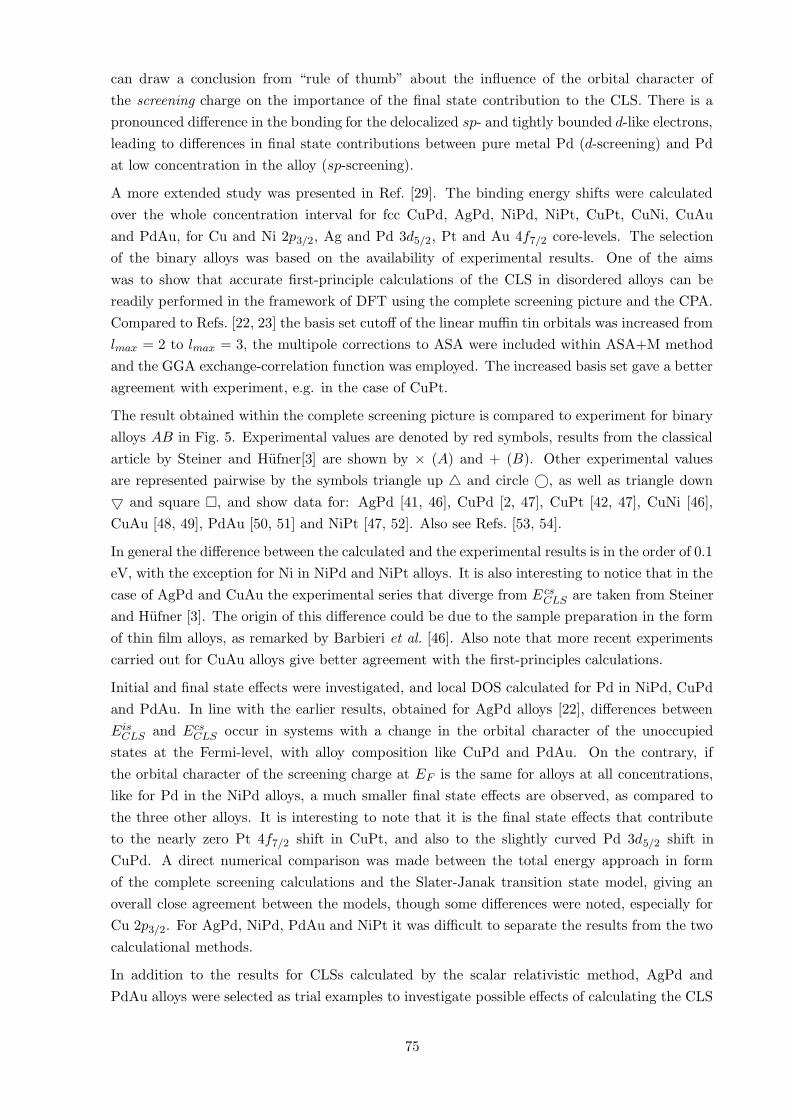
The result obtained within the complete screening picture is compared to experiment for binary

alloys AB in Fig. 5. Experimental values are denoted by red symbols, results from the classical

article by Steiner and Hufner[3] are shown by × (A) and + (B). Other experimental values

are represented pairwise by the symbols triangle up 4 and circle ©, as well as triangle down

5 and square �, and show data for: AgPd [41, 46], CuPd [2, 47], CuPt [42, 47], CuNi [46],

CuAu [48, 49], PdAu [50, 51] and NiPt [47, 52]. Also see Refs. [53, 54].

In general the difference between the calculated and the experimental results is in the order of 0.1

eV, with the exception for Ni in NiPd and NiPt alloys. It is also interesting to notice that in the

case of AgPd and CuAu the experimental series that diverge from E csCLS are taken from Steiner

and Hufner [3]. The origin of this difference could be due to the sample preparation in the form

of thin film alloys, as remarked by Barbieri et al. [46]. Also note that more recent experiments

carried out for CuAu alloys give better agreement with the first-principles calculations.

Initial and final state effects were investigated, and local DOS calculated for Pd in NiPd, CuPd

and PdAu. In line with the earlier results, obtained for AgPd alloys [22], differences between

EisCLS and Ecs

CLS occur in systems with a change in the orbital character of the unoccupied

states at the Fermi-level, with alloy composition like CuPd and PdAu. On the contrary, if

the orbital character of the screening charge at EF is the same for alloys at all concentrations,

like for Pd in the NiPd alloys, a much smaller final state effects are observed, as compared to

the three other alloys. It is interesting to note that it is the final state effects that contribute

to the nearly zero Pt 4f7/2 shift in CuPt, and also to the slightly curved Pd 3d5/2 shift in

CuPd. A direct numerical comparison was made between the total energy approach in form

of the complete screening calculations and the Slater-Janak transition state model, giving an

overall close agreement between the models, though some differences were noted, especially for

Cu 2p3/2. For AgPd, NiPd, PdAu and NiPt it was difficult to separate the results from the two

calculational methods.

In addition to the results for CLSs calculated by the scalar relativistic method, AgPd and

PdAu alloys were selected as trial examples to investigate possible effects of calculating the CLS

75

-0.9-0.6-0.3

00.30.60.91.2

Cor

e-le

vel b

indi

ng e

nerg

y sh

ift (

eV)

-0.9-0.6-0.3

00.30.60.9

-0.9-0.6-0.3

00.30.60.9

10 30 50 70 90

Concentration of B in AB alloy (at. %)

-1.2-0.9-0.6-0.3

00.30.60.9

10 30 50 70 90

Ag

Pd

Ni

Pd

Pd

Cu

Pt

Cu Ni

Pt

Pd

Au

Cu

Au

Cu Ni

Figure 5: CLS in fcc random alloys AgPd, NiPd, CuPd, CuPt, CuNi, CuAu, PdAu and NiPt.

EexpCLS is denoted by disconnected red symbols, Ecs

CLS full line connected blue symbols, E isCLS

dashed green lines for Pd 3d5/2 and Pt 4f7/2. See text for further details.

76

according to fully relativistic theory. Only small differences were noted, which might also be

related to the numerical accuracy of the computations. Core-level shifts were also investigated

in ferromagnetic systems. Substantial effects due to magnetism was observed in CuNi, on Cu

and Ni 2p3/2 CLS for the alloy concentration > 50% of Ni, in agreement with the result from

experiment for both alloy components.

6 Sensitivity of the CLS to local environment effects

6.1 Disorder broadening of core photoemission spectra

A fundamental feature of random alloys is that chemically equivalent atoms are located in dif-

ferent local environments, opposed to the situation in an ordered compound. In the previous

section only results from CPA calculations were considered, that effectively average the local

effects. Binding energies, and hence CLSs, tend to give different values depending on the specific

chemical environment around an atom. With some generalization this would also seem plausible

to hold in the case of different local environments in a random alloy. One of the likely conse-

quences that can be predicted is that the spectral line of a core-level attains a larger width in a

random alloy, if compared to the corresponding line-width in the pure metal. This difference is

called disorder broadening. It is in fact only quite recently in XPS experiments with very high

resolution that disorder broadening has been detected, first for Cu 2p3/2 in fcc CuPd random

alloys by Cole et al. [7], and thereafter the same group has obtained additional results for Cu

2p3/2 in CuPd, CuZn and CuPt, and Ag 3d5/2 in AgPd [41, 53, 55, 56].

6.2 Experimental deduction of disorder broadening

The analysis starts with numerically fitting a Doniach–Sunjic (DS) [57] lineshape to the mea-

sured XPS line of the pure metal. DS lineshapes are characterized by two parameters, the

lifetime parameter and the assymetry index. The DS lineshape is broadened by a Gaussian to

simulate the instrumental broadening. The lineshape parameters are then determined by numer-

ical fitting. Upon alloying one assumes that the lifetime parameter is unchanged, which leaves

the assymetry index as the only parameter to simulate the XPS alloy spectra. A satisfactory

fitting between simulation and experimental data can be obtained by artificially increasing the

Gaussian broadening. This indicates that the additional source of broadening present in alloys,

not included in the simulation, is Gaussian in character. Knowing the instrumental- and the

total broadening mechanism one can isolate and deduce the disorder broadening of the CLS. A

more detailed description can be found in the literature, for instance in Refs. [55, 56].

6.3 A theoretical approach

Disorder broadening was investigated theoretically in Ref. [34], using the complete screening

picture according to Eq. (3) by introducing a single core-ionized atom at a time at each lattice site

in the supercell for the perturbed system. Actual calculations were done by means of the LSGF

approach [16, 17], and by calculations in VASP [18, 19, 20, 21] where additionally the (Z+1)-

77

0.2 0.4 0.6 0.8 1.0

Core−level shift (eV)

Cou

nts

(arb

. uni

ts)

−1.0 −0.6 −0.2 0.2

Ag 3d5/2

Pd 3d5/2

Cu 2p3/2

Pd 3d5/2

Γcs=0.16 eV Γcs

=0.35 eV

Γcs=0.06 eV Γcs

=0.13 eV

(a) CuPd (b) AgPd

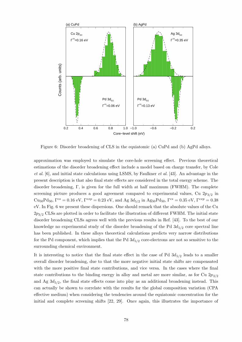
Figure 6: Disorder broadening of CLS in the equiatomic (a) CuPd and (b) AgPd alloys.

approximation was employed to simulate the core-hole screening effect. Previous theoretical

estimations of the disorder broadening effect include a model based on charge transfer, by Cole

et al. [6], and initial state calculations using LSMS, by Faulkner et al. [43]. An advantage in the

present description is that also final state effects are considered in the total energy scheme. The

disorder broadening, Γ, is given for the full width at half maximum (FWHM). The complete

screening picture produces a good agreement compared to experimental values, Cu 2p3/2 in

Cu50Pd50, Γcs = 0.16 eV, Γexp = 0.23 eV, and Ag 3d5/2 in Ag50Pd50, Γcs = 0.35 eV, Γexp = 0.38

eV. In Fig. 6 we present these dispersions. One should remark that the absolute values of the Cu

2p3/2 CLSs are plotted in order to facilitate the illustration of different FWHM. The initial state

disorder broadening CLSs agrees well with the previous results in Ref. [43]. To the best of our

knowledge no experimental study of the disorder broadening of the Pd 3d5/2 core spectral line

has been published. In these alloys theoretical calculations predicts very narrow distributions

for the Pd component, which implies that the Pd 3d5/2 core-electrons are not so sensitive to the

surrounding chemical environment.

It is interesting to notice that the final state effect in the case of Pd 3d5/2 leads to a smaller

overall disorder broadening, due to that the more negative initial state shifts are compensated

with the more positive final state contributions, and vice versa. In the cases where the final

state contributions to the binding energy in alloy and metal are more similar, as for Cu 2p3/2

and Ag 3d5/2, the final state effects come into play as an additional broadening instead. This

can actually be shown to correlate with the results for the global composition variation (CPA

effective medium) when considering the tendencies around the equiatomic concentration for the

initial and complete screening shifts [22, 29]. Once again, this illustrates the importance of

78

including final state effetcs in the analysis of CLSs. For more details see Ref. [34].

Moreover, the influence of local lattice relaxations on the CLS in the CuPd alloy was studied

by means of the projected-augmented wave [58, 59] (PAW) method, implemented in VASP. We

find that the average CLS, for both components, remain the same when we allow for the local

lattice relaxations compared to an unrelaxed underlying lattice. Considering the average CLS

as a function of nearest neighbors (NNs) of the opposite kind in the first coordination shell, we

find that close to the equiatomic distribution the unrelaxed and relaxed lattice gives the same

CLS. However, deviations from local equiatomic compositions causes differences in the average

CLS per NN, resulting in an increased disorder broadening. The FWHM parameter Γ increases

by 0.04 eV and 0.06 eV for Cu and Pd respectively comparing to calculations for unrelaxed

and relaxed underlying lattice. Allowing the bond length in the random alloy to relax really

brings the theoretical results in better agreement with experiment. The effect of increasing

FWHM due to local lattice relaxations was also suggested by Faulkner and co-workers in their

theoretical study [43]. Local lattice relaxations might be of more importance for systems with

larger size-mismatch between the atoms that constitute the alloy.

7 Interface structures

The interest in studying interface core-level shift (IFCLS) is motivated by possible applications.

For instance, a question can be asked if it is possible to detect any difference between whole

embedded metal monolayers and various stages of intermixing – or a completely disordered

sample. This further leads to the question if theoretically predicted differences between interface

qualities could be detected in experimental measurements (with a sufficiently high resolution).

If so, theoretical IFCLSs could be used in conjunction with experiment to assist the structure

characterization of complex materials.

From a theoretical point of view, it is straightforward to model systems in question, calculate

IFCLSs and make a direct comparison. This was done for some trial structures in Refs. [31, 32].

For our calculations of surface and interfaces, the Green’s function technique [14] was employed.

No steps and no surface or local lattice relaxation was permitted, which is usually a reasonable

approximation considering the aim, which is to capture general trends. In particular, the above

assumption allows for relatively fast calculations, especially compared to supercell methods.

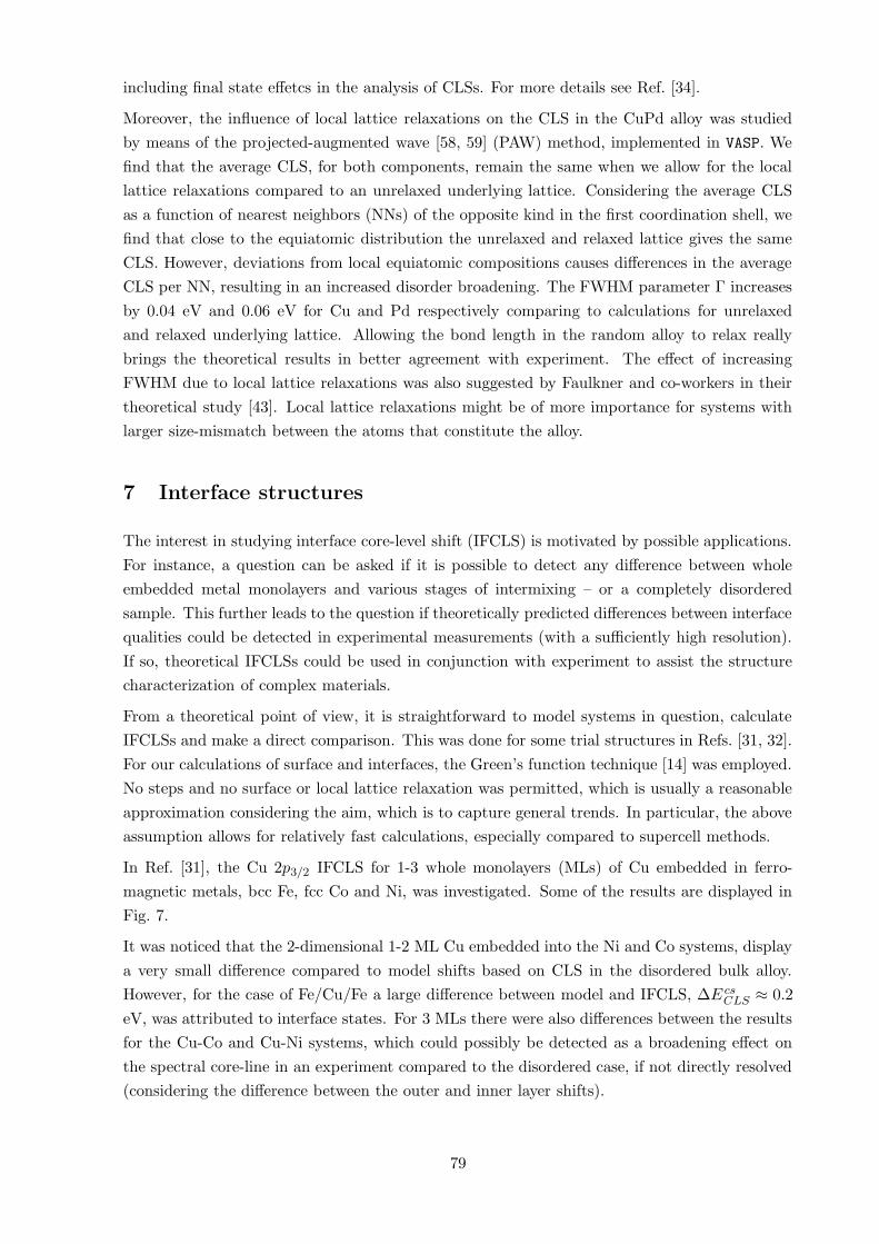
In Ref. [31], the Cu 2p3/2 IFCLS for 1-3 whole monolayers (MLs) of Cu embedded in ferro-

magnetic metals, bcc Fe, fcc Co and Ni, was investigated. Some of the results are displayed in

Fig. 7.

It was noticed that the 2-dimensional 1-2 ML Cu embedded into the Ni and Co systems, display

a very small difference compared to model shifts based on CLS in the disordered bulk alloy.

However, for the case of Fe/Cu/Fe a large difference between model and IFCLS, ∆E csCLS ≈ 0.2

eV, was attributed to interface states. For 3 MLs there were also differences between the results

for the Cu-Co and Cu-Ni systems, which could possibly be detected as a broadening effect on

the spectral core-line in an experiment compared to the disordered case, if not directly resolved

(considering the difference between the outer and inner layer shifts).

79

1 2 3 bulkLayers of Cu

-0.2

-0.1

0

0.1

0.2

0.3

Inte

rfac

e co

re-l

evel

shi

ft (

eV)

fcc Ni/Cu/Nifcc Co/Cu/Cobcc Fe/Cu/Fe

Figure 7: Layer resolved Cu 2p3/2 IFCLS (eV) for 1-3 MLs of Cu in Me/Cu/Me, Me = Ni, Co

and Fe. Cu bulk CLSs at volume of the surrounding metals is given on the right hand side.

Dashed lines are drawn between inner layer shifts for 3 MLs and bulk CLS, the remaining IFCLS

for 3 MLs represents the outer layer shift.

In the further work [32], a more extensive theoretical study is made regarding the Cu 2p3/2

IFCLS for the bcc Fe/Cu/Fe, fcc Co/Cu/Co and Ni/Cu/Ni systems. Here the Cu layers vary

in thickness between 1-10 MLs, for the cases of no intermixing and two choices of interface

qualities. Different trends are captured for the systems. While in Ni/Cu/Ni a large spread is

found in the IFCLSs over the total number of Cu layers and at different degrees of intermixing,

which would seem possible to detect experimentally, the effect is smaller in Co/Cu/Co. As in

Ref. [31], the results for the Fe/Cu/Fe systems differ from the other systems. It is found that

the effect on Cu CLS exists at the sharp Fe-Cu interfaces (no intermixing), and is attributed to

interface states, mentioned above. The latter disappear with mixing of Fe and Cu.

To summarize, while it has been shown that theoretical results for layer resolved interface core-

level shifts are readily calculated, it would be of high interest to investigate the experimental

detectability of different interface qualities in future work.

8 Thin film surface structures

In Refs. [24, 30] take into account applicational aspects of the theoretical determination of

core-level shifts for the case of thin film surface structures, attempting their structural charac-

terization based on the comparison between calculated and experimental measurements.

Indeed, in Ref [60] measured binding energy shifts of Pd 3d5/2 were presented in the near surface

region of Pd(100) with a thin magnetic layer of Mn; 1 ML Mn on Pd(100) and a PdMn overlayer

on top, obtained by annealing. One of the interesting questions that arised was the determination

of the annealed structure.

As in the case of interface structures in the previous section, the surface and interface Green’s

80

function technique was used. As a first test of the accuracy of the complete screening pic-

ture computations, SCLSs were calculated and compared with experiment for the case of pure

Pd(100) and the 1 ML Mn/Pd(100) system. It was found that theory gave reasonable shifts

compared with experiment and previous calculations in the literature. In the experiment it was

deducted that Mn formed ‘checkerboard’ pattern (C) together with Pd (P ) in a layer, resulting

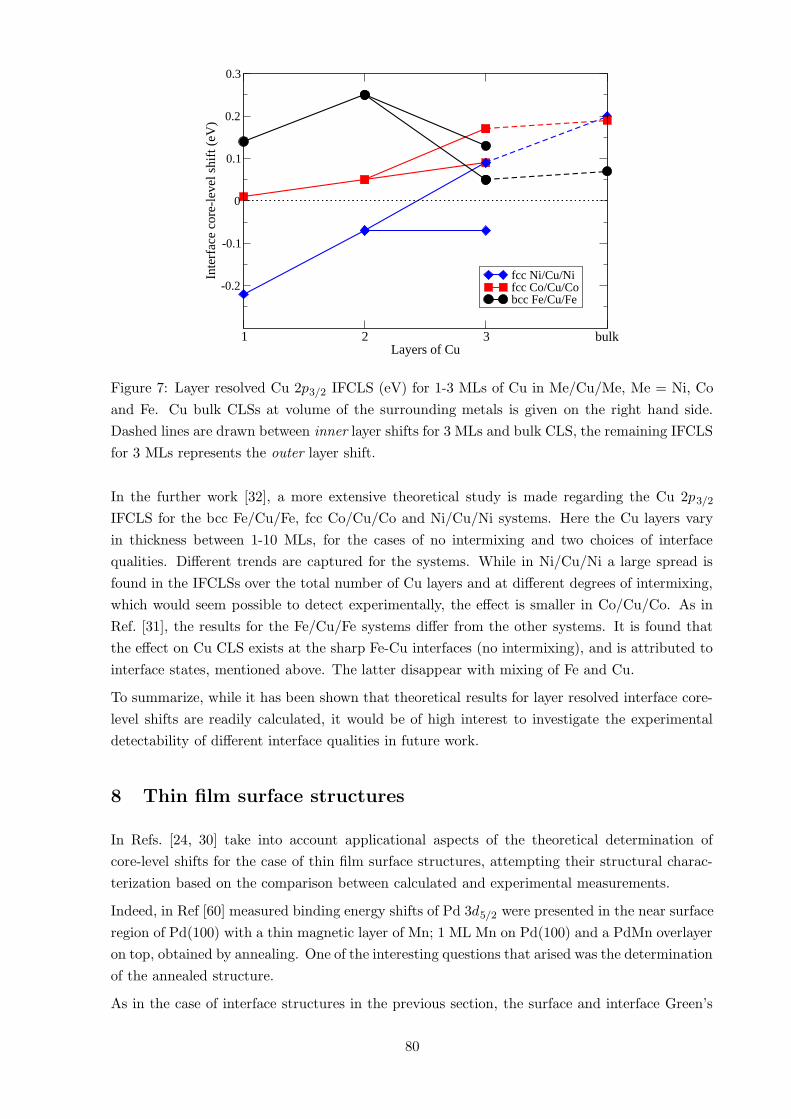
in 2 C-layers after annealing. In Ref. [24] experimental results were compared to the theory by

calculating the near surface CLSs of Pd for the candidate systems suggested in Ref. [60], namely

I C/C, II C/P/C and III P/C/P/C on Pd(100), see Fig. 8.

The layer resolved CLS compared to experiment is displayed in Fig. 8, layers are numbered from

the surface, S, and downwards. In addition, the difference in total energy, ∆E, against a 1 ML

Mn/Pd(100) system is given. From the figure it is indeed very easy to single out the structure I as

the one reached after annealing. A direct comparison between the experimental and theoretical

SCLSs, clearly leads to this conclusion. One sees that the presence of Mn atoms in a layer leads

to a significantly different CLS at the Pd atoms. For instance notice the differences between

the CLS at the surface Pd atoms as Mn goes deeper into the bulk. Also notice that structure I

has a higher total energy as compared with the energetically more favourable structures II and

III. They are however not formed due to kinetic limitations [60]. A natural extension of the

study would be to continue the annealing of PdMn/Pd(100), and make a further comparison

between theory and experiment. In brief, this example shows the possibility to use theoretical

CLSs together with experimental results to make a prediction for metastable structures obtained

in experiment.

In Ref. [30], this idea was further investigated in a combined theoretical and experimental study

Figure 8: Layer resolved Pd 3d5/2 CLS (eV) for the PdMn/Pd(100) structures I. - III. Pd

(white spheres) and Mn (black spheres) with arrows indicating the magnetic moment. ∆E gives

difference in total energy compared to a 1 ML Mn/Pd(100) system. All values are given in eV.

81

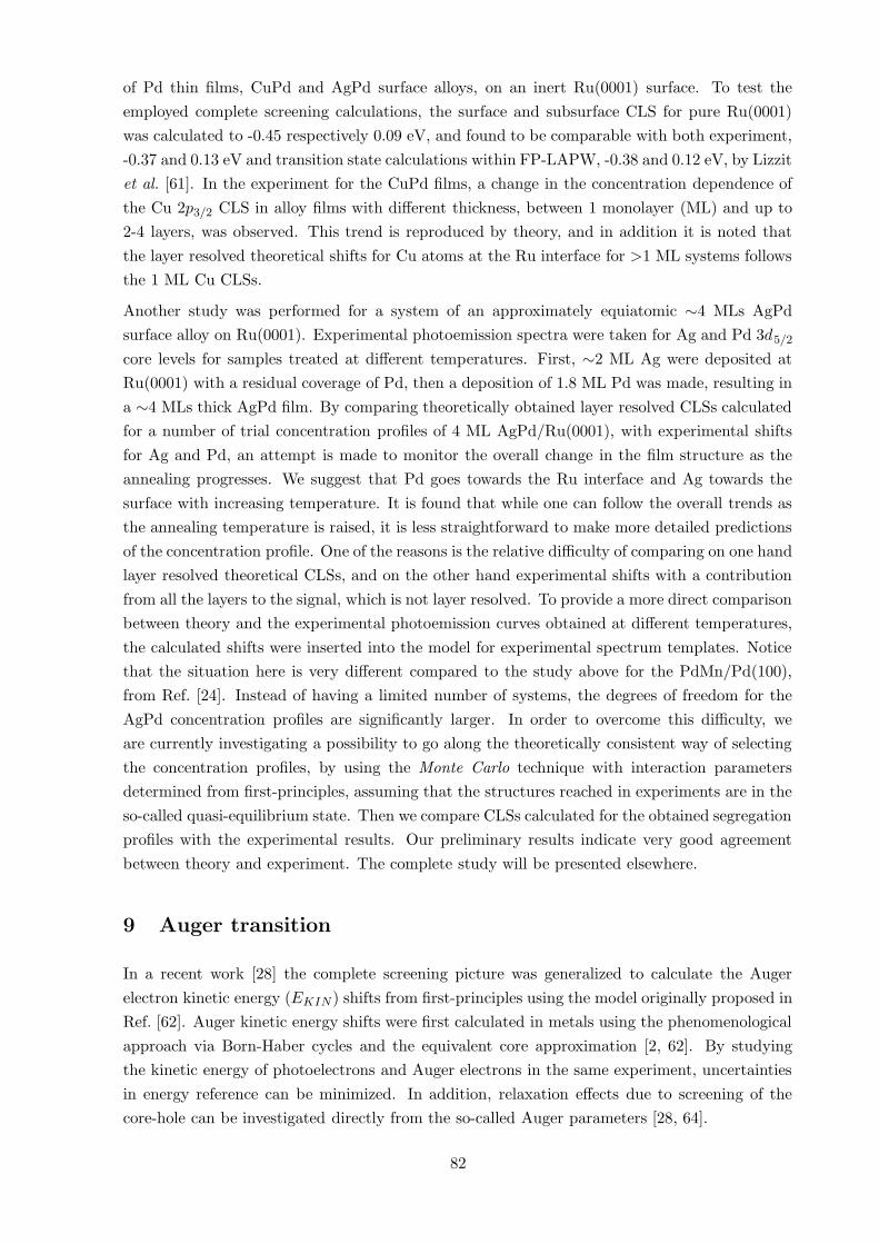
of Pd thin films, CuPd and AgPd surface alloys, on an inert Ru(0001) surface. To test the

employed complete screening calculations, the surface and subsurface CLS for pure Ru(0001)

was calculated to -0.45 respectively 0.09 eV, and found to be comparable with both experiment,

-0.37 and 0.13 eV and transition state calculations within FP-LAPW, -0.38 and 0.12 eV, by Lizzit

et al. [61]. In the experiment for the CuPd films, a change in the concentration dependence of

the Cu 2p3/2 CLS in alloy films with different thickness, between 1 monolayer (ML) and up to

2-4 layers, was observed. This trend is reproduced by theory, and in addition it is noted that

the layer resolved theoretical shifts for Cu atoms at the Ru interface for >1 ML systems follows

the 1 ML Cu CLSs.

Another study was performed for a system of an approximately equiatomic ∼4 MLs AgPd

surface alloy on Ru(0001). Experimental photoemission spectra were taken for Ag and Pd 3d5/2

core levels for samples treated at different temperatures. First, ∼2 ML Ag were deposited at

Ru(0001) with a residual coverage of Pd, then a deposition of 1.8 ML Pd was made, resulting in

a ∼4 MLs thick AgPd film. By comparing theoretically obtained layer resolved CLSs calculated

for a number of trial concentration profiles of 4 ML AgPd/Ru(0001), with experimental shifts

for Ag and Pd, an attempt is made to monitor the overall change in the film structure as the

annealing progresses. We suggest that Pd goes towards the Ru interface and Ag towards the

surface with increasing temperature. It is found that while one can follow the overall trends as

the annealing temperature is raised, it is less straightforward to make more detailed predictions

of the concentration profile. One of the reasons is the relative difficulty of comparing on one hand

layer resolved theoretical CLSs, and on the other hand experimental shifts with a contribution

from all the layers to the signal, which is not layer resolved. To provide a more direct comparison

between theory and the experimental photoemission curves obtained at different temperatures,

the calculated shifts were inserted into the model for experimental spectrum templates. Notice

that the situation here is very different compared to the study above for the PdMn/Pd(100),

from Ref. [24]. Instead of having a limited number of systems, the degrees of freedom for the

AgPd concentration profiles are significantly larger. In order to overcome this difficulty, we

are currently investigating a possibility to go along the theoretically consistent way of selecting

the concentration profiles, by using the Monte Carlo technique with interaction parameters

determined from first-principles, assuming that the structures reached in experiments are in the

so-called quasi-equilibrium state. Then we compare CLSs calculated for the obtained segregation

profiles with the experimental results. Our preliminary results indicate very good agreement

between theory and experiment. The complete study will be presented elsewhere.

9 Auger transition

In a recent work [28] the complete screening picture was generalized to calculate the Auger

electron kinetic energy (EKIN) shifts from first-principles using the model originally proposed in

Ref. [62]. Auger kinetic energy shifts were first calculated in metals using the phenomenological

approach via Born-Haber cycles and the equivalent core approximation [2, 62]. By studying

the kinetic energy of photoelectrons and Auger electrons in the same experiment, uncertainties

in energy reference can be minimized. In addition, relaxation effects due to screening of the

core-hole can be investigated directly from the so-called Auger parameters [28, 64].

82

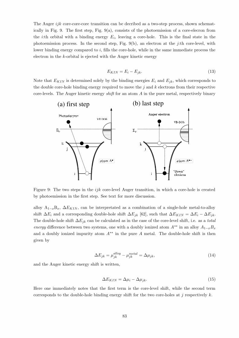
The Auger ijk core-core-core transition can be decribed as a two-step process, shown schemat-

ically in Fig. 9. The first step, Fig. 9(a), consists of the photoemission of a core-elecron from

the i:th orbital with a binding energy Ei, leaving a core-hole. This is the final state in the

photoemission process. In the second step, Fig. 9(b), an electron at the j:th core-level, with

lower binding energy compared to i, fills the core-hole, while in the same immediate process the

electron in the k-orbital is ejected with the Auger kinetic energy

EKIN = Ei −Ejk. (13)

Note that EKIN is determined solely by the binding energies Ei and Ejk, which corresponds to

the double core-hole binding energy required to move the j and k electrons from their respective

core-levels. The Auger kinetic energy shift for an atom A in the pure metal, respectively binary

Figure 9: The two steps in the ijk core-level Auger transition, in which a core-hole is created

by photoemission in the first step. See text for more discussion.

alloy A1−xBx, ∆EKIN , can be interpretated as a combination of a single-hole metal-to-alloy

shift ∆Ei and a corresponding double-hole shift ∆Ejk [62], such that ∆EKIN = ∆Ei − ∆Ejk.

The double-hole shift ∆Ejk can be calculated as in the case of the core-level shift, i.e. as a total

energy difference between two systems, one with a doubly ionized atom A∗∗ in an alloy A1−xBx

and a doubly ionized impurity atom A∗∗ in the pure A metal. The double-hole shift is then

given by

∆Ejk = µalloyjk − µmetal

jk = ∆µjk, (14)

and the Auger kinetic energy shift is written,

∆EKIN = ∆µi − ∆µjk. (15)

Here one immediately notes that the first term is the core-level shift, while the second term

corresponds to the double-hole binding energy shift for the two core-holes at j respectively k.

83

10 30 50 70 90Concentration Pd (at. %)

−1.5

−1

−0.5

0

0.5

−1

−0.5

0

0.5

1

Bin

ding

ene

rgy

shift

(eV

)

AgPdLMM

∆µL

∆µMM

∆ξ exp. ∆ξ

(a)

(b)

Ag

Pd

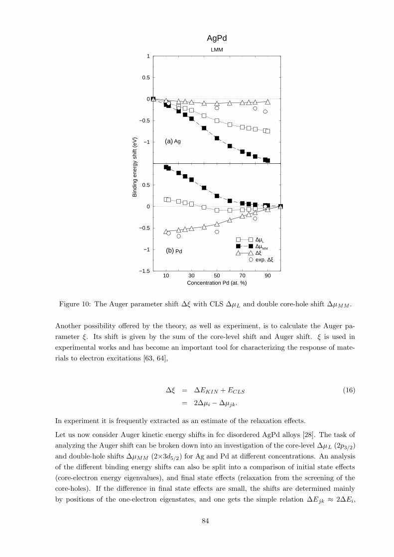
Figure 10: The Auger parameter shift ∆ξ with CLS ∆µL and double core-hole shift ∆µMM .

Another possibility offered by the theory, as well as experiment, is to calculate the Auger pa-

rameter ξ. Its shift is given by the sum of the core-level shift and Auger shift. ξ is used in

experimental works and has become an important tool for characterizing the response of mate-

rials to electron excitations [63, 64],

∆ξ = ∆EKIN +ECLS (16)

= 2∆µi − ∆µjk.

In experiment it is frequently extracted as an estimate of the relaxation effects.

Let us now consider Auger kinetic energy shifts in fcc disordered AgPd alloys [28]. The task of

analyzing the Auger shift can be broken down into an investigation of the core-level ∆µL (2p3/2)

and double-hole shifts ∆µMM (2×3d5/2) for Ag and Pd at different concentrations. An analysis

of the different binding energy shifts can also be split into a comparison of initial state effects

(core-electron energy eigenvalues), and final state effects (relaxation from the screening of the

core-holes). If the difference in final state effects are small, the shifts are determined mainly

by positions of the one-electron eigenstates, and one gets the simple relation ∆Ejk ≈ 2∆Ei,

84

because deeply laying core states feel a change of the crystal potential as a rigid shift. In this

case one obtains ∆µMM ≈ 2∆µL, leading to very simple anti-symmetry relation between the

Auger kinetic energy shift and the core-level shift, ∆EKIN = ∆µL −∆µMM ≈ −∆µL. This can

be confirmed in the case of Ag by inspecting the theoretical results, and is due to that the Ag

core holes are screened by mainly sp electrons both, in alloys and in the pure metal [28].

In Fig. 10 the separate contributions to the Auger kinetic energy and the Auger parameter

shifts in fcc AgPd alloys, Eqs. (15) and (16), respectively, are shown, the calculated metal-to-

alloy changes of the chemical potentials of single ionized atoms ∆µL, as well as that for double

ionized atoms ∆µMM , together with the Auger parameter shift. Good agreement between theory

and experiment is observed for the Auger parameters shifts. Also, one can clearly see a relation,

∆µMM ≈ 2∆µL, in the case of Ag, as discussed above. In the case of Pd the relation does not

hold, indicating larger importance of of the relaxation effects, in agreement with larger value of

the Auger parameter shift.

10 Summary

An overview is presented for the recent work on first-principles studies of core-level binding

energy shifts, mainly using the complete screening picture, which includes initial and final state

effects in the same computational scheme. Investigations have been made for various types of

complex systems, including a number of disordered alloys, interface structures and thin films on

surfaces, with good agreement between theoretical and experimental results (when available).

Initial state CLSs were used to estimate the final state effects. The complete screening picture,

which is a total energy approach, was compared to the transition state model, an energy eigen-

value approach which however also includes both initial and final state effects. It was found

that the agreement is typically very good between the two different methods. An improvement

for the use of the transition state model was suggested with minimal increase of computational

costs. In addition to the study of CLS as a function of the alloy composition within the coherent

potential approximation (which gives fast computation), results were obtained for the broad-

ening of the spectral core-line due to the different local chemical environments in a disordered

alloy, by using supercell methods. We also propose to using theoretical shifts together with ex-

perimental data as a tool for structural charaterization of materials. For instance we applied the

methodology for the structural characterization of metastable samples obtained in experiment,

as well as for the determination of the interface qualities. The continued development of x-ray

photoelectron spectroscopy towards increased resolution, encourages both a direct comparison

between experiment and theory, as well as an investigation of applicational purposes – using

theory and experiment together.

Acknowledgements

We are grateful to the Swedish Research Council (VR) and the Swedish Foundation for Strategic

Research (SSF) for the financial support. We are also grateful to our collaborators on the

projects reviewed in this article, Prof. B. Johansson, Prof. P. Weightman, Prof. R. J. Cole,

85

Prof. J. Onsgaard, Dr. E. Holmstrom and Dr. A. M. N. Niklasson. Calculations has been

performed at the High Performance Computing Center North (HPC2N) in Umea, Sweden, and

at the National Supercomputer Centre (NSC) in Linkoping, Sweden.

References

[1] B. Johansson and N. Martensson, Phys. Rev. B 21, 4427 (1980).

[2] N. Martensson, R. Nyholm, H. Calen, J. Hedman, and B. Johansson, Phys. Rev. B 24,

1725 (1981).

[3] P. Steiner and S. Hufner, Acta Metall. 29, 1885 (1981).

[4] A. Rosengren and B. Johansson, Phys. Rev. B 23, 3852 (1981).

[5] U. Gelius, Phys. Scr. 9, 133 (1974).

[6] R. J. Cole, N. J. Brooks and P. Weightman, Phys. Rev. B 56, 12178 (1997).

[7] R. J. Cole, N. J. Brooks and P. Weightman, Phys. Rev. Lett. 78, 3777 (1997).

[8] M. Weinert and R. E. Watson, Phys. Rev. B 51, 17168 (1995).

[9] S. Hufner, Photoelectron Spectroscopy, Principles and Applications (Springer-Verlag Berlin,

2003), 3rd ed.

[10] W.F. Egelhoff, Jr., Surface Science Reports 6, 253 (1987).

[11] P. Hohenberg and W. Kohn, Phys. Rev. 136, B864 (1964).

[12] W. Kohn and L.J. Sham, Phys. Rev. 140, A1133 (1965).

[13] I.A. Abrikosov and H.L. Skriver, Phys. Rev. B 47, 16532 (1993).

[14] A.V. Ruban and H.L. Skriver, Comput. Mater. Sci. 15, 119 (1999).

[15] H.L. Skriver and N.M. Rosengaard, Phys. Rev. B 43, 9538 (1991).

[16] I.A. Abrikosov, A.M.N. Niklasson, S.I. Simak, B. Johansson, A.V. Ruban, and H.L. Skriver,

Phys. Rev. Lett. 76, 4203 (1996).

[17] I.A. Abrikosov, S.I. Simak, B. Johansson, A.V. Ruban, and H.L. Skriver, Phys. Rev. B 56,

9319 (1997).

[18] G. Kresse, and J. Hafner, Phys. Rev. B 47, R558 (1993).

[19] G. Kresse, and J. Hafner, Phys. Rev. B 49, 14251 (1994).

[20] G. Kresse, and J. Furthmuller, Comput. Mater. Sci. 6, 15 (1996).

[21] G. Kresse, and J. Furthmuller, Phys. Rev. B 54, 11169 (1996).

[22] I. A. Abrikosov, W. Olovsson, and B. Johansson, Phys. Rev. Lett. 87, 176403 (2001).

86

[23] W. Olovsson, I. A. Abrikosov, and B. Johansson, J. Electron Spectrosc. Relat. Phenom.

127, 65 (2002).

[24] W. Olovsson, E. Holmstrom, A. Sandell, and I. A. Abrikosov, Phys. Rev. B 68, 045411

(2003).

[25] L. V. Pourovskii, A. V. Ruban, I. A. Abrikosov, Yu. Kh. Vekilov, and B. Johansson, JETP

Lett. 73, 415 (2001).

[26] L. V. Pourovskii, A. V. Ruban, I. A. Abrikosov, Yu. Kh. Vekilov, and B. Johansson, Phys.

Rev. B 64, 035421 (2001).

[27] L. V. Pourovskii, A. V. Ruban, B. Johansson, and I. A. Abrikosov, Phys. Rev. Lett. 90,

026105 (2003).

[28] W. Olovsson, I. A. Abrikosov, B. Johansson, A. Newton, R. J. Cole, and P. Weightman,

Phys. Rev. Lett. 92, 226406 (2004).

[29] W. Olovsson, C. Goransson, L.V. Pourovskii, B. Johansson, and I.A. Abrikosov, Phys. Rev.

B 72, 064203 (2005).

[30] W. Olovsson, L. Bech, T.H. Andersen, Z. Li, S.V. Hoffmann, B. Johansson, I.A. Abrikosov,

and J. Onsgaard, Phys. Rev. B 72, 075444 (2005).

[31] W. Olovsson, E. Holmstrom, J. Wills, P. James, I.A. Abrikosov, and A.M.N. Niklasson,

Phys. Rev. B 72, 155419 (2005).

[32] W. Olovsson, E. Holmstrom, J. Wills, I.A. Abrikosov, and A.M.N. Niklasson, in manuscript

[33] C. Goransson, W. Olovsson, and I.A. Abrikosov, Phys. Rev. B 72, 134203 (2005).

[34] T. Marten, W. Olovsson, S.I. Simak, and I.A. Abrikosov, Phys. Rev. B 72, 054210 (2005).

[35] M. Alden, H. L. Skriver, and B. Johansson, Phys. Rev. Lett. 71, 2449 (1993).

[36] M. Alden, I. A. Abrikosov, B. Johansson, N. M. Rosengaard, and H. L. Skriver, Phys. Rev.

B 50, 5131 (1994).

[37] A.V. Ruban and H.L. Skriver, Phys. Rev. B 55, 8801 (1997).

[38] A. Stierle, C. Tieg, H. Dosch, V. Formoso, E. Lundgren, J.N. Andersen, L. Kohler, and G.

Kresse. Surf. Sci. 529, L263.

[39] J. F. Janak, Phys. Rev. B 18, 7165 (1978).

[40] J.C. Slater, Quantum theory of molecules and solids, vol. 4 of International series in Pure

and Applied physics (McGraw-Hill, 1974), 1st ed.

[41] A.W. Newton, S. Haines, P. Weightman, and R.J. Cole, J. Electron Spetrosc. Relat. Phe-

nom. 136, 235 (2004).

[42] Y.-S. Lee, K.-Y Lim, Y.-D. Chung, C.-N. Whang, and Y. Jeon, Surf. Interface Anal. 30,

475 (2000).

87

[43] J.S. Faulkner, Y. Wang and G.M. Stocks, Phys. Rev. Lett. 81, 1905 (1998).

[44] N. Martensson and A. Nilsson, J. Electron Spectrosc. Relat. Phenom. 75, 209 (1995).

[45] M. Methfessel, V. Fiorentini, and S. Oppo, Phys. Rev. B 61, 5229 (2000).

[46] P.F. Barbieri, A. de Siervo, M.F. Carazolle, R. Landers, and G.G. Kleiman, J. Electron

Spetrosc. Relat. Phenom. 135, 113 (2004).

[47] A.W. Newton. Charge Transfer and Disorder Broadening in Disordered Transition Metal

Alloys. PhD thesis, University of Liverpool, 2001.

[48] M. Kuhn and T.K. Sham, Phys. Rev. B 49, 1647 (1994).

[49] T.K. Sham, A. Hiraya, and M. Watanabe, Phys. Rev. B 55, 7585 (1997).

[50] P.A.P. Nascente, S.G.C. de Castro, R. Landers, and G.G. Kleiman, Phys. Rev. B 43, 4659

(1991).

[51] Y.-S. Lee, Y. Jeon, Y.-D. Chung, K.-Y. Lim, C.-N. Whang, and S.-J. Oh, J. Korean Phys.

Soc. 37, 451 (2000).

[52] E. Choi, S.-J. Oh, and M. Choi, Phys. Rev. B 43, 6360 (1991).

[53] A.W. Newton, A. Vaughan, R.J. Cole, and P. Weightman, J. Electron Spetrosc. Relat.

Phenom. 107, 185 (2000).

[54] S.R. Haines, A.W. Newton, and P. Weightman, J. Electron Spetrosc. Relat. Phenom. 137-

40, 429 (2004).

[55] R.J. Cole, and P. Weightman, J. Phys. Cond. Matt. 10, 5679 (1998).

[56] D. Lewis, R.J. Cole, and P. Weightman J. Phys. Cond. Matt. 11, 8431 (1999).

[57] S. Doniach, and M. Sunjic, J. Phys. C: Solid State Phys. 3, 285 (1970).

[58] P.E. Blochl, Phys. Rev. B 50, 17953 (1994).

[59] G. Kresse, and D. Joubert, Phys. Rev. B 59, 1758 (1999).

[60] A. Sandell, P.H. Andersson, E. Holmstrom, A.J. Jaworowski, and L. Nordstrom, Phys. Rev.

B 65, 035410 (2001).

[61] S. Lizzit, A. Baraldi, A. Groso, K. Reuter, M.V. Ganduglia-Pirovano, C. Stampfl, M.

Scheffler, M. Stichler, C. Keller, W. Wurth, and D. Menzel, Phys. Rev. B 63, 205419

(2001).

[62] N. Martensson, P. Hedegard and B. Johansson, Phys. Scr. 29, 154 (1984).

[63] N. D. Lang and A. R. Williams, Phys. Rev. B 20, 1369 (1979).

[64] G. Moretti, J. Electron Spectrosc. Relat. Phenom. 95, 95 (1998).

88