Copyright © Cengage Learning. All rights reserved.

2 Limits and Derivatives

Copyright © Cengage Learning. All rights reserved.

2.2 The Limit of a Function

33

The Limit of a Function

To find the tangent to a curve or the velocity of an object,

we now turn our attention to limits in general and numerical

and graphical methods for computing them.

Let’s investigate the behavior of the function f defined by

f (x) = x2 – x + 2 for values of x near 2.

44

The Limit of a Function

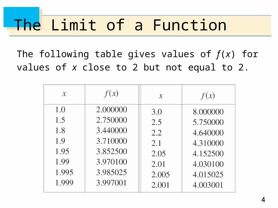
The following table gives values of f (x) for values of x close

to 2 but not equal to 2.

55

The Limit of a Function

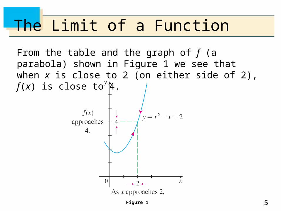
From the table and the graph of f (a parabola) shown in Figure 1 we see that when x is close to 2 (on either side of 2), f (x) is close to 4.

Figure 1

66

The Limit of a Function

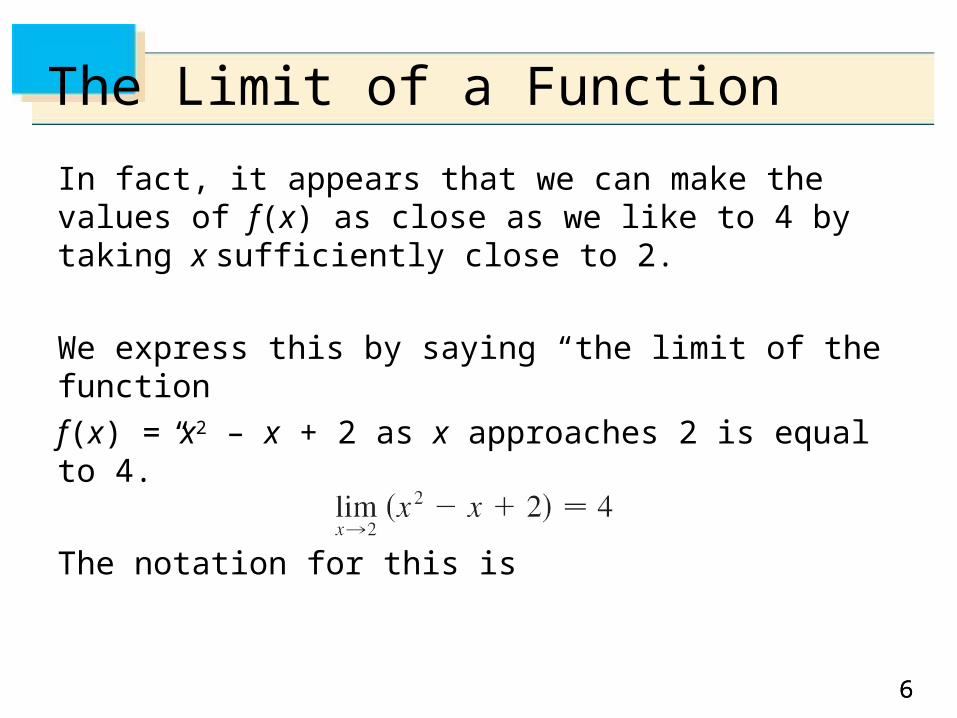
In fact, it appears that we can make the values of f (x) as close as we like to 4 by taking x sufficiently close to 2.

We express this by saying “the limit of the function

f (x) = x2 – x + 2 as x approaches 2 is equal to 4.”

The notation for this is

77

The Limit of a Function

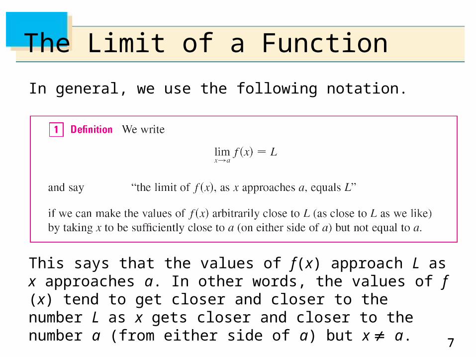
In general, we use the following notation.

This says that the values of f (x) approach L as x approaches a. In other words, the values of f (x) tend to get closer and closer to the number L as x gets closer and closer to the number a (from either side of a) but x a.

88

The Limit of a Function

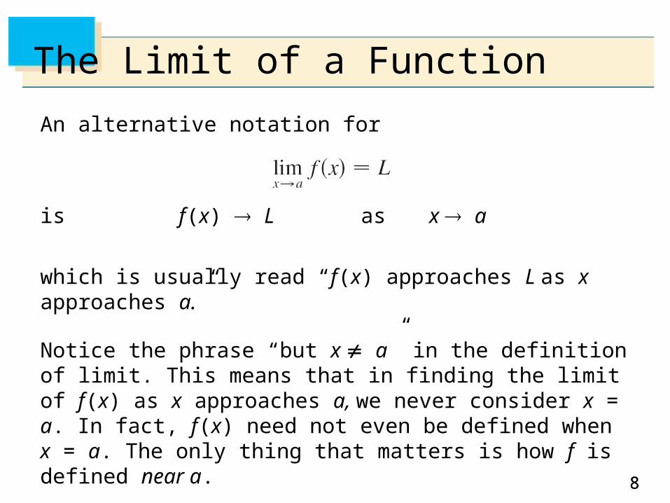
An alternative notation for

is f (x) L as x a

which is usually read “f (x) approaches L as x approaches a.”

Notice the phrase “but x a” in the definition of limit. This means that in finding the limit of f (x) as x approaches a, we never consider x = a. In fact, f (x) need not even be defined when x = a. The only thing that matters is how f is defined near a.

99

The Limit of a Function

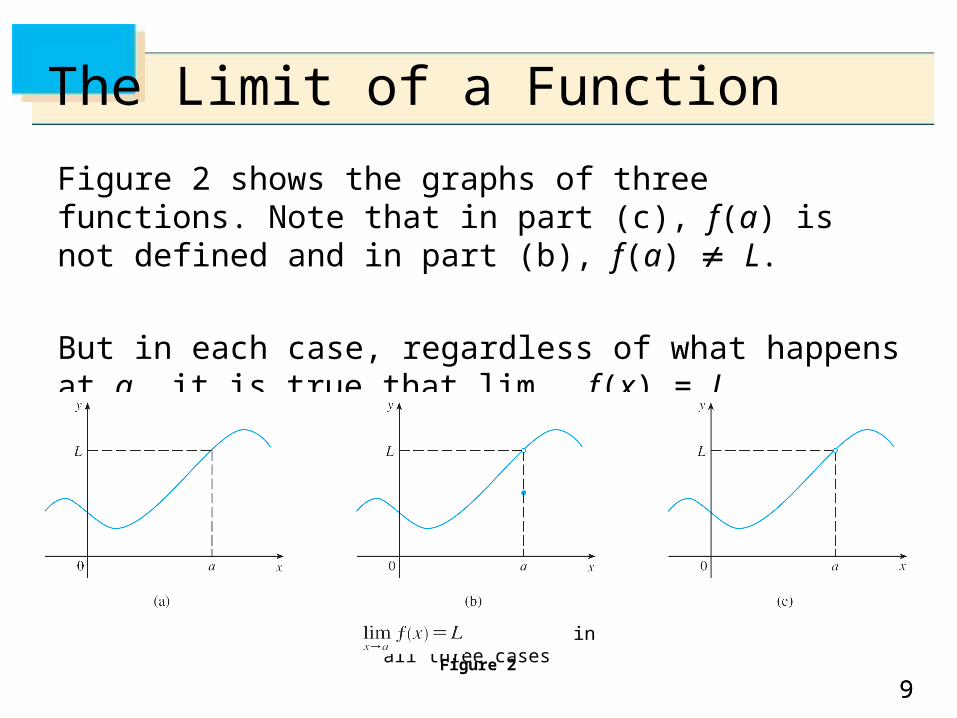
Figure 2 shows the graphs of three functions. Note that in part (c), f (a) is not defined and in part (b), f (a) L.

But in each case, regardless of what happens at a, it is true that limxa f (x) = L.

Figure 2

in all three cases

1010

Example 1

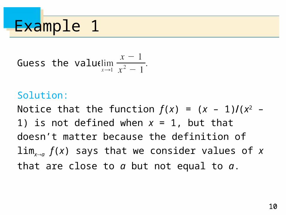
Guess the value of

Solution:

Notice that the function f (x) = (x – 1)(x2 – 1) is not defined

when x = 1, but that doesn’t matter because the definition

of limxa f (x) says that we consider values of x that are

close to a but not equal to a.

1111

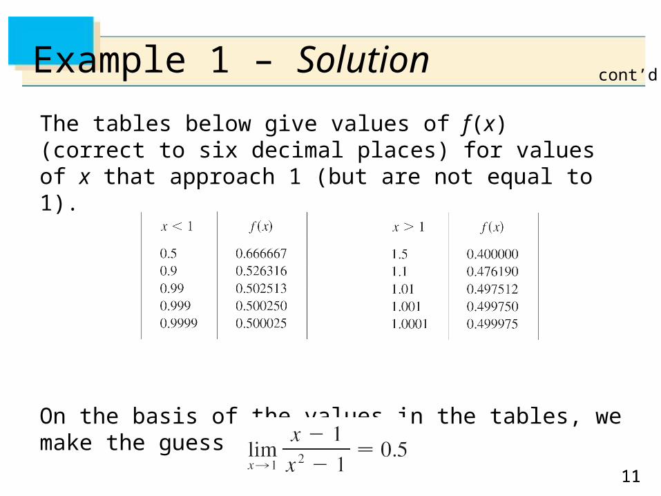
Example 1 – Solution

The tables below give values of f (x) (correct to six decimal places) for values of x that approach 1 (but are not equal to 1).

On the basis of the values in the tables, we make the guess that

cont’d

1212

The Limit of a Function

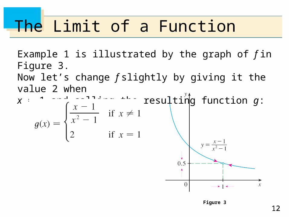
Example 1 is illustrated by the graph of f in Figure 3. Now let’s change f slightly by giving it the value 2 whenx = 1 and calling the resulting function g:

Figure 3

1313

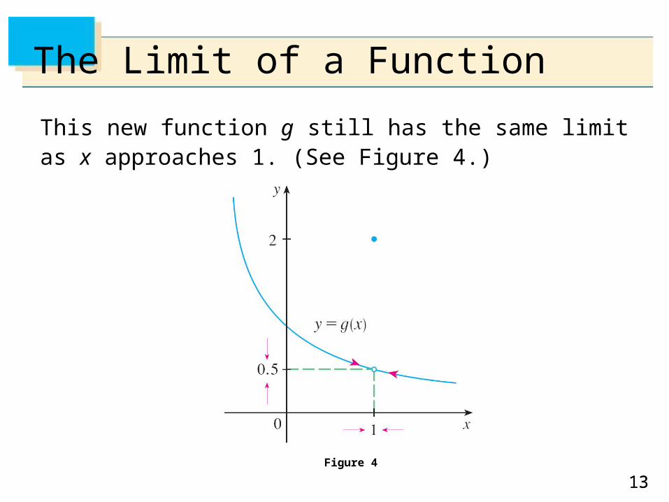
The Limit of a Function

This new function g still has the same limit as x approaches 1. (See Figure 4.)

Figure 4

1414

One-Sided Limits

1515

One-Sided Limits

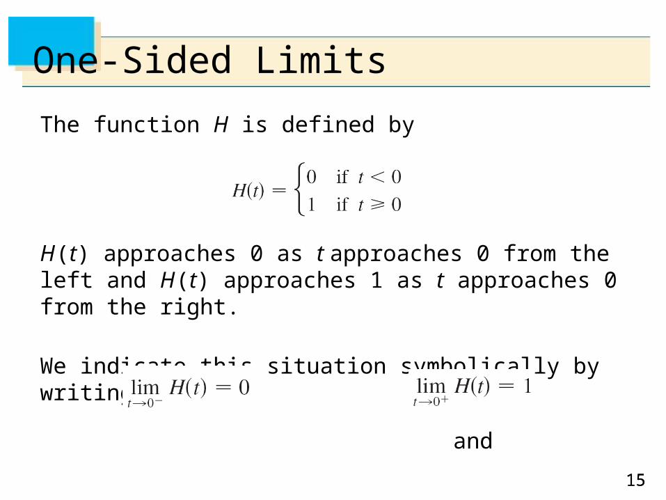
The function H is defined by

.

H (t) approaches 0 as t approaches 0 from the left and H (t) approaches 1 as t approaches 0 from the right.

We indicate this situation symbolically by writing

and

1616

One-Sided Limits

The symbol “t 0–” indicates that we consider only values

of t that are less than 0.

Likewise, “t 0+” indicates that we consider only values of t

that are greater than 0.

1717

One-Sided Limits

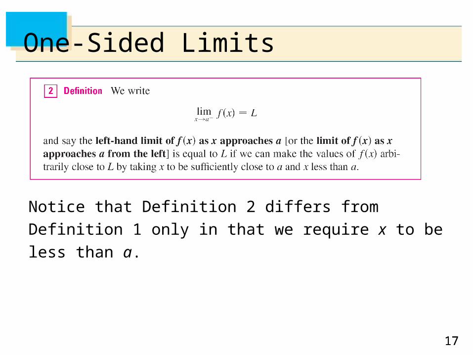
Notice that Definition 2 differs from Definition 1 only in that

we require x to be less than a.

1818

One-Sided Limits

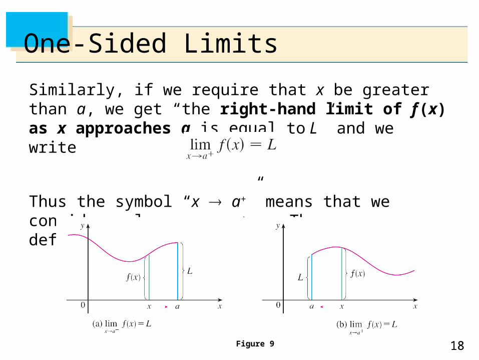
Similarly, if we require that x be greater than a, we get “the right-hand limit of f (x) as x approaches a is equal to L” and we write

Thus the symbol “x a+” means that we consider only x > a. These definitions are illustrated in Figure 9.

Figure 9

1919

One-Sided Limits

By comparing Definition 1 with the definitions of one-sided

limits, we see that the following is true.

2020

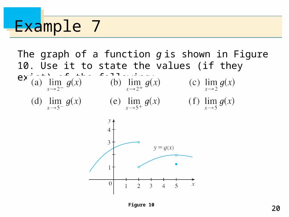
Example 7

The graph of a function g is shown in Figure 10. Use it to state the values (if they exist) of the following:

Figure 10

2121

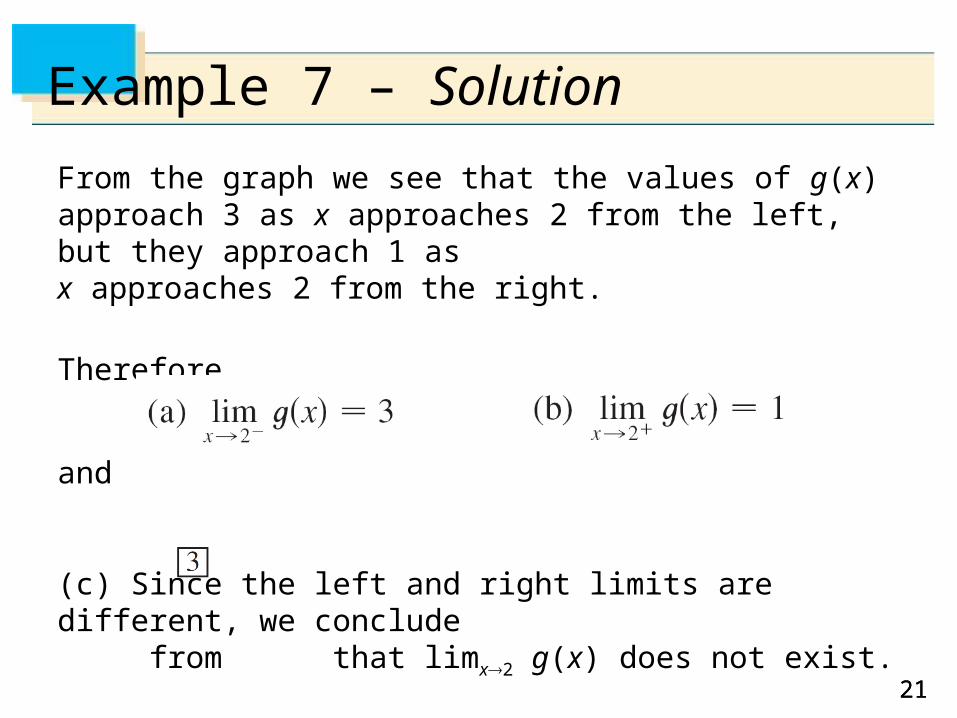
Example 7 – Solution

From the graph we see that the values of g(x) approach 3 as x approaches 2 from the left, but they approach 1 asx approaches 2 from the right.

Therefore

and

(c) Since the left and right limits are different, we conclude from that limx2 g(x) does not exist.

2222

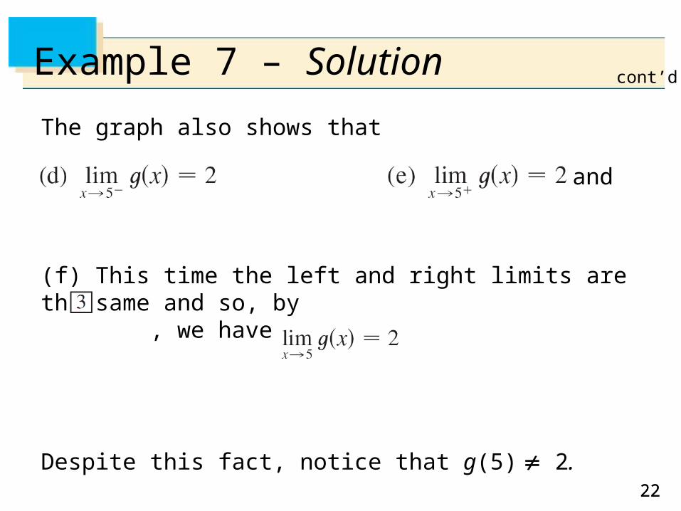
Example 7 – Solution

The graph also shows that

and

(f) This time the left and right limits are the same and so, by , we have

Despite this fact, notice that g(5) 2.

cont’d

2323

Infinite Limits

2424

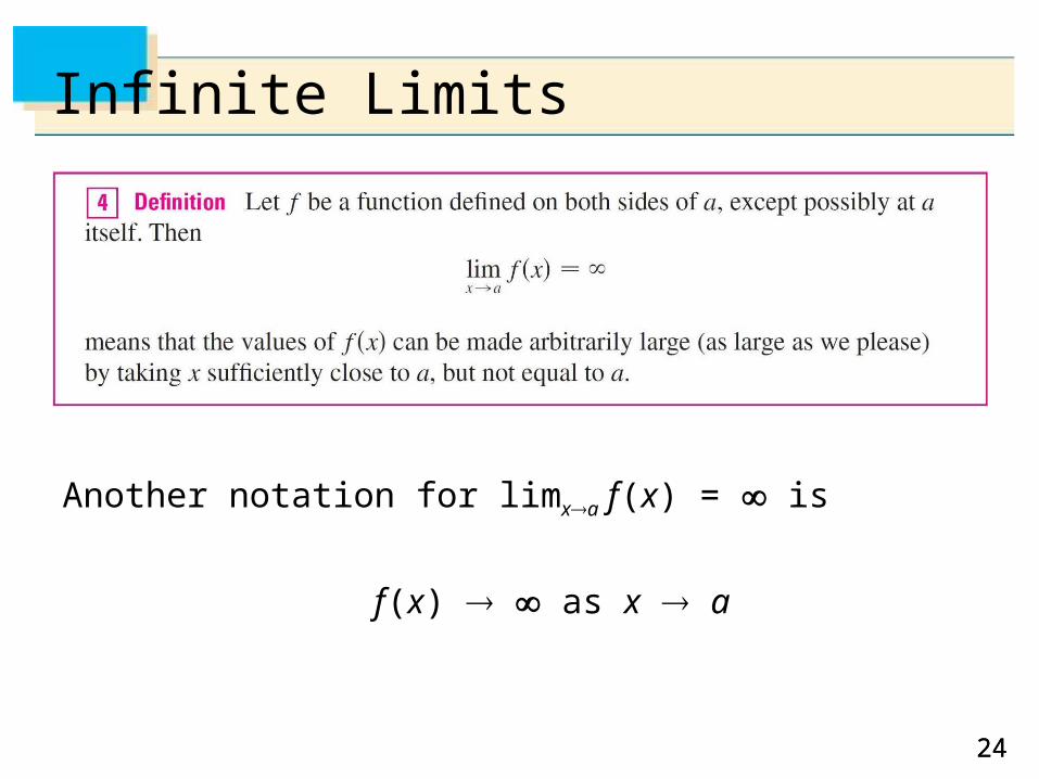
Infinite Limits

Another notation for limxa f (x) = is

f (x) as x a

2525

Again, the symbol is not a number, but the expression limxa f (x) = is often read as

“the limit of f (x), as approaches a, is infinity”

or “f (x) becomes infinite as approaches a”

or “f (x) increases without bound as approaches a”

Infinite Limits

2626

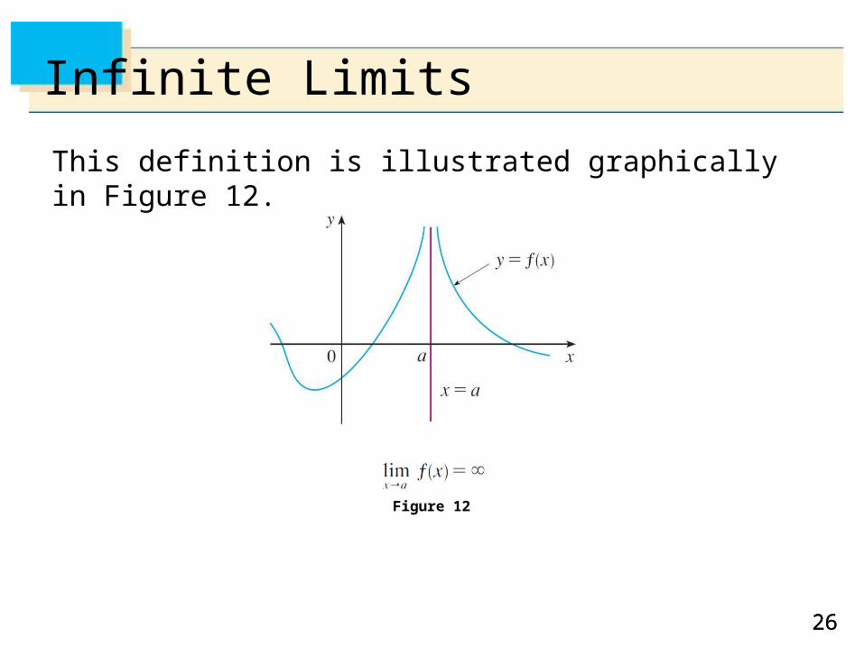
This definition is illustrated graphically in Figure 12.

Figure 12

Infinite Limits

2727

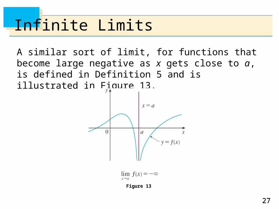
A similar sort of limit, for functions that become large negative as x gets close to a, is defined in Definition 5 and is illustrated in Figure 13.

Figure 13

Infinite Limits

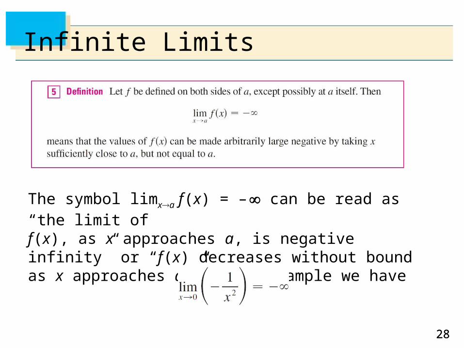
2828

The symbol limxa f (x) = – can be read as “the limit of f (x), as x approaches a, is negative infinity” or “f (x) decreases without bound as x approaches a.” As an example we have

Infinite Limits

2929

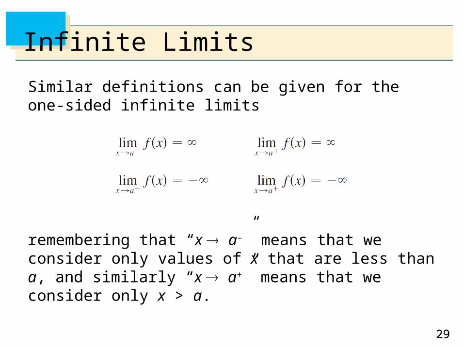
Similar definitions can be given for the one-sided infinite limits

remembering that “x a–” means that we consider only values of x that are less than a, and similarly “x a+” means that we consider only x > a.

Infinite Limits

3030

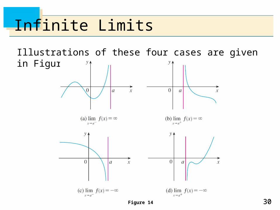
Illustrations of these four cases are given in Figure 14.

Infinite Limits

Figure 14

3131

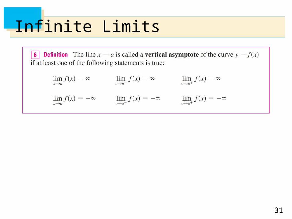
Infinite Limits

3232

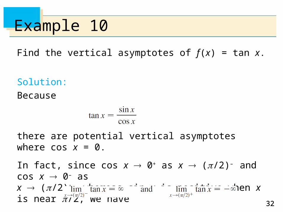
Find the vertical asymptotes of f (x) = tan x.

Solution:

Because

there are potential vertical asymptotes where cos x = 0.

In fact, since cos x 0+ as x ( /2)– and cos x 0– as x ( /2)+, whereas sin x is positive when x is near /2, we have

Example 10

3333

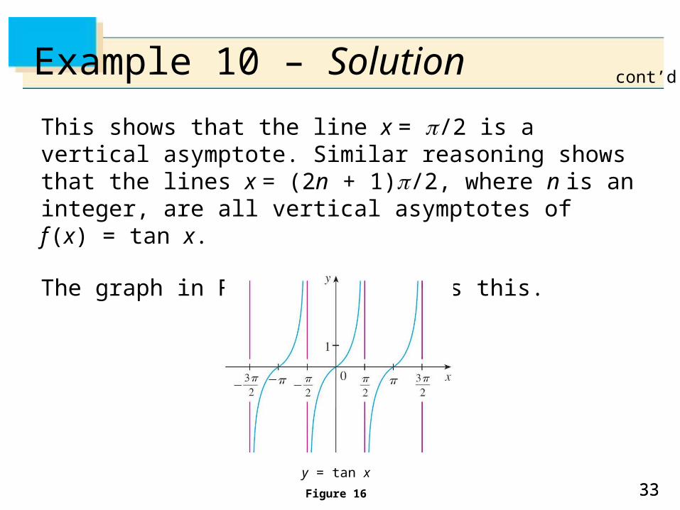
This shows that the line x = /2 is a vertical asymptote. Similar reasoning shows that the lines x = (2n + 1) /2, where n is an integer, are all vertical asymptotes off (x) = tan x.

The graph in Figure 16 confirms this.

Example 10 – Solution

y = tan x

Figure 16

cont’d