Copyright (c) Bani Mallick1 STAT 651 Lecture # 11.
45
Copyright (c) Bani Mallic k 1 STAT 651 Lecture # 11
-
date post
22-Dec-2015 -
Category
Documents
-
view
215 -
download
1
Transcript of Copyright (c) Bani Mallick1 STAT 651 Lecture # 11.

Copyright (c) Bani Mallick 1
STAT 651
Lecture # 11

Copyright (c) Bani Mallick 2
Topics in Lecture #11 Comparing two population means
Review to date

Copyright (c) Bani Mallick 3
Book Sections Covered in Lecture #11
All previous chapters
Copyright (c) Bani Mallick 4
Lecture 10 Review: Robust Inference via Rank Tests
Because sample means and sd’s are sensitive to outliers, so too are comparisons of populations based on them
Rank tests form a robust alternative, that can be used to check the results of t-statistic inferences
You are looking for major discrepancies, and then trying to explain them

Copyright (c) Bani Mallick 5
Lecture 10 Review: Robust Inference via Rank Tests
Typically called the Wilcoxon rank sum test
The algorithm is to assign ranks to each observation in the pooled data set
Then apply a t-test to these ranks
Robust because ranks can never get wild

Copyright (c) Bani Mallick 6
Lecture 10 Review: Robust Inference via Rank Tests
The rank tests give the same answer no matter whether you take the raw data, their logarithms or their square roots.
If you have data (raw or transformed) that pass q-q plots tests, then Wilcoxon and t-test should have much the same p-values
In this case, you can use the latter to get CI’s

Copyright (c) Bani Mallick 7
Lecture 10 Review: Inference for Equality of Variances
SPSS uses what is called Levene’s test
From the SPSS Help file (slightly edited)
Levene Test
For each case, it computes the absolute difference between the value of that case and its cell mean and performs a t-test on those absolute differences.
Copyright (c) Bani Mallick 8
Inference When the Variances Are Not Equal
Generally, you should try to find a scale (log, square root) for which the variances are approximately equal.
If you cannot, then a small change is needed in the confidence intervals and test statistics.
Copyright (c) Bani Mallick 9
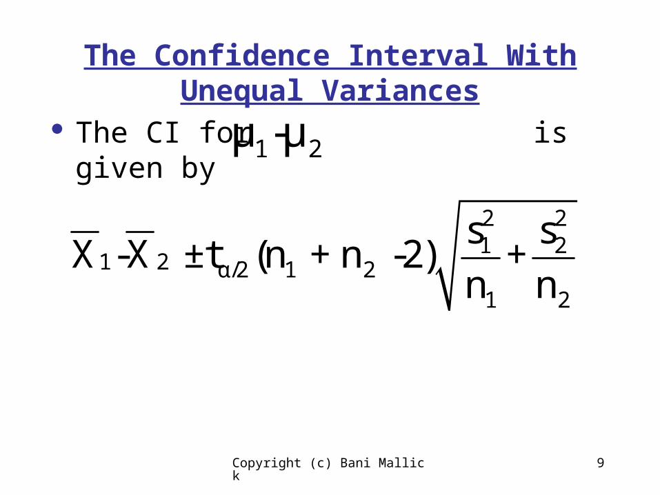
The Confidence Interval With Unequal Variances
The CI for is given by
2 21 2
1 2 α/2 1 21 2
s sX -X ±t (n + n -2) +
n n
1 2μ -μ

Copyright (c) Bani Mallick 10
The t-test Statistic With Unequal Variances
The t-statistic is defined by
1 2
2 21 2
1 2
X Xt =
s s
n n

Copyright (c) Bani Mallick 11
The Aortic Stenosis Data: A Review
Let’s remember that the aortic stenosis data is comparing healthy with sick kids
Aortic Valve Area (AVA) and Body Surface Area (BSA) are noninvasive measures
The idea is to see if we can use these measures to understand whether a kid is stenotic, without having to do an invasive test
Or at least to be able to narrow down those who need an invasive test

Copyright (c) Bani Mallick 12
The Aortic Stenosis Data: A Review
We will study the variable log(1 + AVA/BSA)
I’ll try to review much of what we have done to this point by using these data
There was a kids with an enormous AVA: I’ll delete this kid from all analyses
First comes the relative frequency histogram
Copyright (c) Bani Mallick 13
The Aortic Stenosis Data: A Review
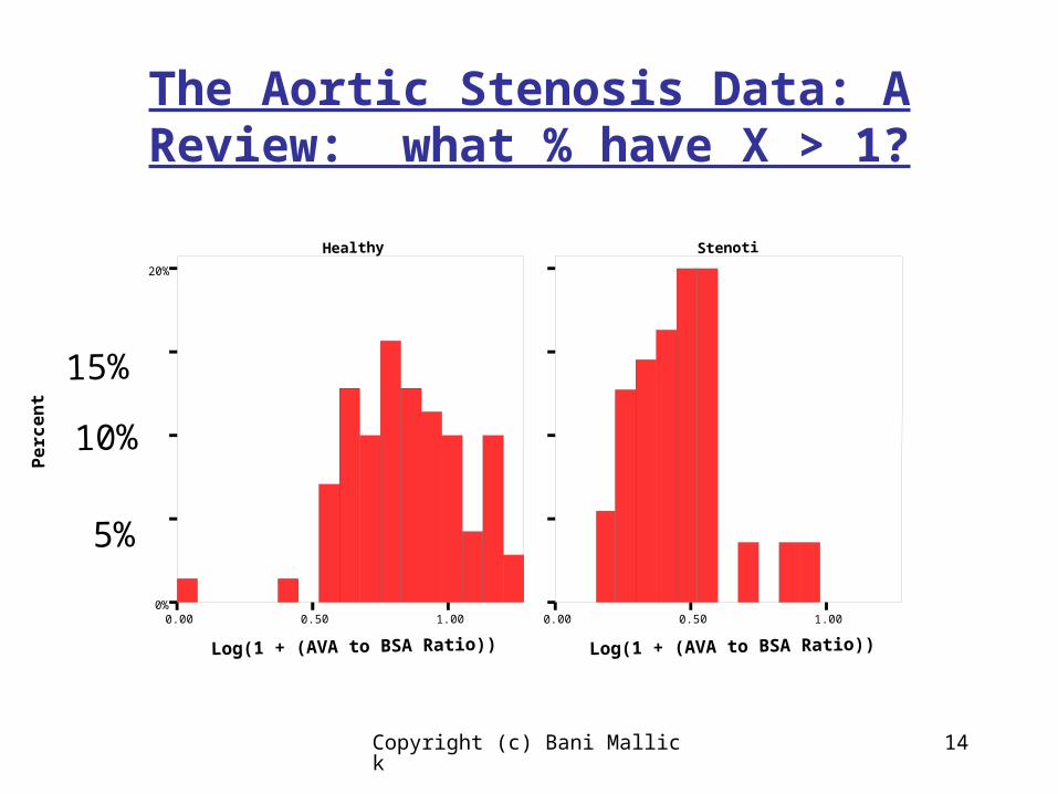
First comes the relative frequency histogram
The height of each bar is the % of the sample which lies in the interval for that bar
Copyright (c) Bani Mallick 14
The Aortic Stenosis Data: A Review: what % have X > 1?
0.00 0.50 1.00
Log(1 + (AVA to BSA Ratio))
0%
5%
10%
15%
20%
Pe
rce
nt
Healthy Stenoti
0.00 0.50 1.00
Log(1 + (AVA to BSA Ratio))

Copyright (c) Bani Mallick 15
The Aortic Stenosis Data: A Review
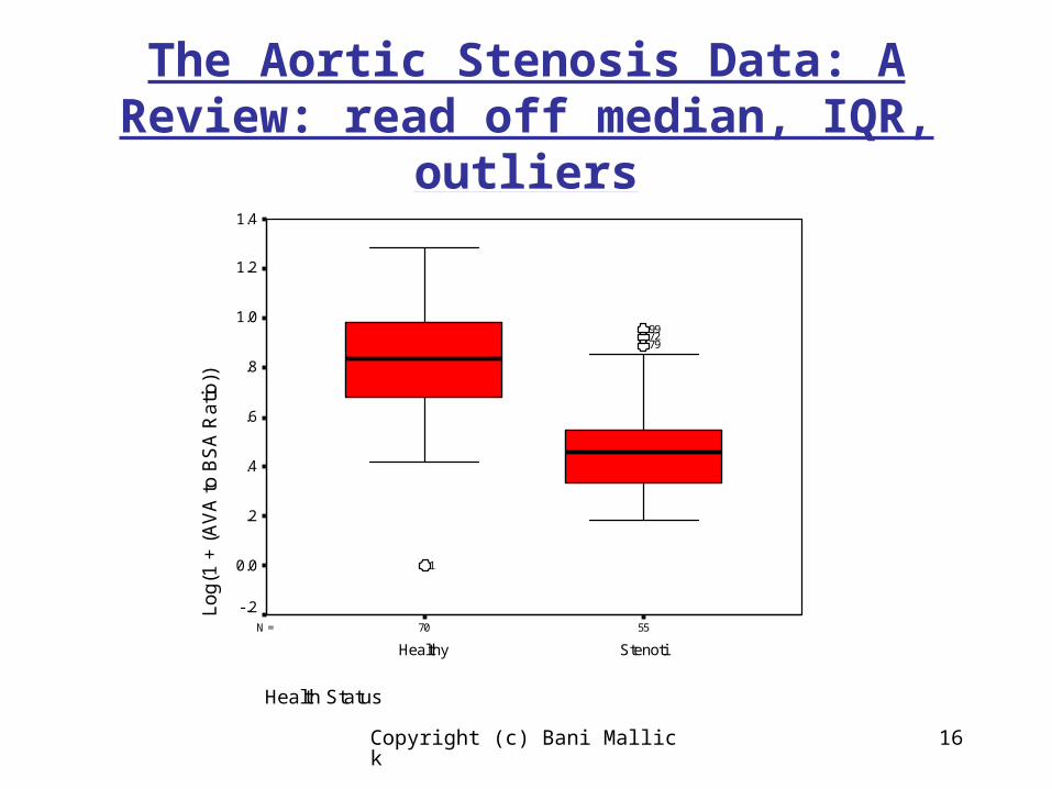
Next comes the boxplot to
Compare medians
Compare variability
Screen for massive outliers
Copyright (c) Bani Mallick 16
The Aortic Stenosis Data: A Review: read off median, IQR,
outliers
5570N =
Health Status
StenotiHealthy
Lo
g(1
+ (
AV
A t
o B
SA
Ra
tio))
1.4
1.2
1.0
.8
.6
.4
.2
0.0
-.2
797299
1
Copyright (c) Bani Mallick 17
The Aortic Stenosis Data: A Review
Next comes the q-q plot to check for approximate bell-shape
Why does it matter that the data are approximately bell-shaped?
First: statistical inferences such as confidence intervals are most accurate and most powerful
Second: Probability calculations are most accurate

Copyright (c) Bani Mallick 18
The Aortic Stenosis Data: A Review
For the healthy kids: what do you think?
Normal Q-Q Plot of Log(1 + (AVA to BSA Ratio))
Observed Value
1.41.21.0.8.6.4.20.0-.2
Exp
ect
ed
No
rma
l Va
lue
1.4
1.2
1.0
.8
.6
.4
.2

Copyright (c) Bani Mallick 19
The Aortic Stenosis Data: A Review
For the stenotic kids: what do you think?
Normal Q-Q Plot of Log(1 + (AVA to BSA Ratio))
Observed Value
1.0.8.6.4.20.0
Exp
ect
ed
No
rma
l Va
lue
1.0
.8
.6
.4
.2
0.0

Copyright (c) Bani Mallick 20
The Aortic Stenosis Data: A Review
Next we do some simple summary statistics
Healthy: n = 70, mean = 0.84, median = 0.83, sd = 0.22, iqr = 0.31, se (of mean) = 0.026
Stenotic: n = 55, mean = 0.47, median = 0.46, sd = 0.17, iqr = 0.22, se (of mean) = 0.023
What does the IQR mean?

Copyright (c) Bani Mallick 21
The Aortic Stenosis Data: A Review
Healthy: n = 70, mean = 0.84, median = 0.83, sd = 0.22, iqr = 0.31, se (of mean) = 0.026
Degrees of freedom = 70 – 1 = 69
95% CI for population mean (from SPSS) = 0.79 to 0.89
Interpret this!

Copyright (c) Bani Mallick 22
The Aortic Stenosis Data: A Review
Healthy: n = 70, mean = 0.84, median = 0.83, sd = 0.22, iqr = 0.31, se (of mean) = 0.026
Estimate the probability that a healthy child has a log(1+ASA/BSA) less that 0.46
Pr(X < 0.46): z-score = (0.46 – 0.84)/0.22 = -1.73
Table 1: Pr(X < 0.46) ~ 0.0418
Interpret this!
Copyright (c) Bani Mallick 23
The Aortic Stenosis Data: A Review
Note: for computing confidence intervals for the population mean I use the standard error
In computing probabilities about the population I use the standard deviation
Which one is affected by the sample size?

Copyright (c) Bani Mallick 24
The Aortic Stenosis Data: A Review
Next I will compare the population means
We have concluded that the data are fairly (although not exactly) normally distributed
We have also concluded that the variabilities are not too awfully different, although the stenotic kids appear to be less variable.
So, we will try out the t-test type inference

Copyright (c) Bani Mallick 25
The Aortic Stenosis Data: A Review
SPSS computes a confidence interval for the difference in the population means
We conclude the population means are different if the confidence interval does not include zero
0 1 2 a 1 2H :μ -μ =0 vs H :μ -μ 0
Copyright (c) Bani Mallick 26
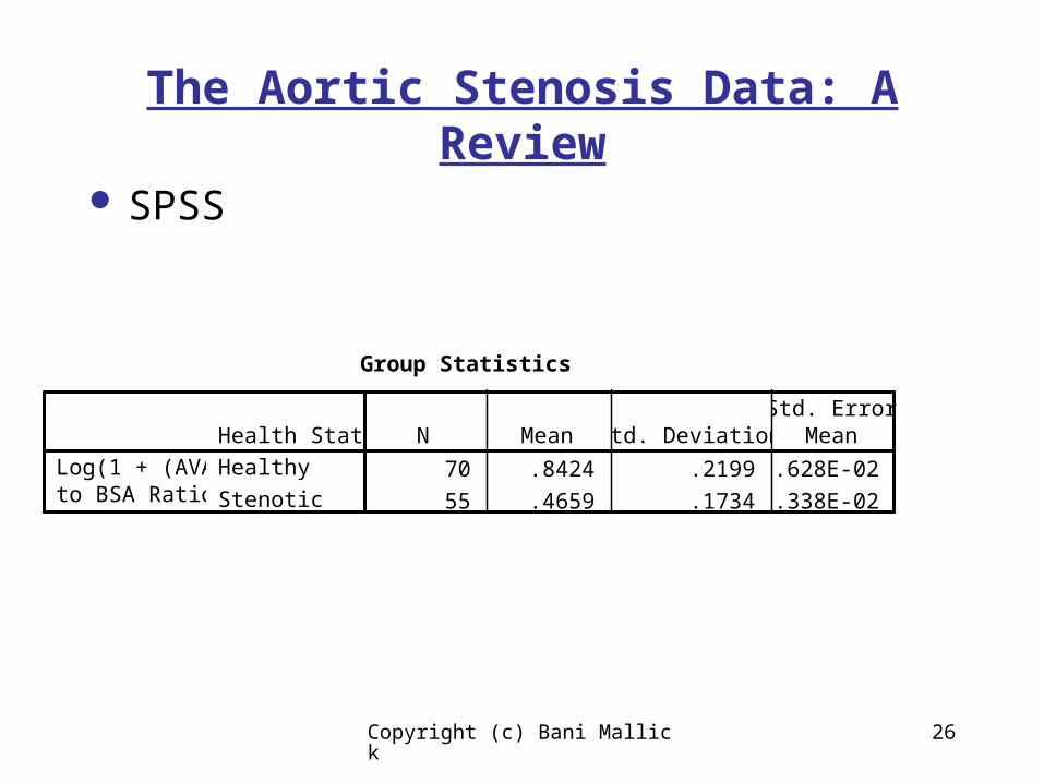
The Aortic Stenosis Data: A Review
SPSS
Group Statistics
70 .8424 .2199 2.628E-02
55 .4659 .1734 2.338E-02
Health StatusHealthy
Stenotic
Log(1 + (AVAto BSA Ratio))
N Mean Std. DeviationStd. Error
Mean

Copyright (c) Bani Mallick 27
The Aortic Stenosis Data: A Review
SPSS
Independent Samples Test
3.346 .070 10.407 123 .000 .3765 3.618E-02 .3049 .4482
10.705 122.997 .000 .3765 3.518E-02 .3069 .4462
Equal variancesassumed
Equal variancesnot assumed
Log(1 + (AVAto BSA Ratio))
F Sig.
Levene's Test forEquality of Variances
t df Sig. (2-tailed)Mean
DifferenceStd. ErrorDifference Lower Upper
95% ConfidenceInterval of the
Difference
t-test for Equality of Means

Copyright (c) Bani Mallick 28
The Aortic Stenosis Data: A Review
The 95% confidence interval is from 0.30 to 0.45
Interpret this!

Copyright (c) Bani Mallick 29
The Aortic Stenosis Data: A Review
The p-value is 0.000.
Interpret this! What would have happened if I had done a 99% CI?
Copyright (c) Bani Mallick 30
The Aortic Stenosis Data: A Review
The p-value is 0.000.
Interpret this! What would have happened if I had done a 99% CI?
It would not have covered zero, and I would have rejected the null hypothesis that the two population means are the same.

Copyright (c) Bani Mallick 31
The Aortic Stenosis Data: A Review
Outliers can really mess up an analysis
We use the Wilcoxon rank sum test for this
There were no massive outliers, the data were nearly normal, so we expect to get just about the same p-value
It is 0.000, just as for the CI analysisTest Statisticsa
305.500
1845.500
-8.055
.000
Mann-Whitney U
Wilcoxon W
Z
Asymp. Sig. (2-tailed)
Log(1 + (AVAto BSA Ratio))
Grouping Variable: Health Statusa.
Copyright (c) Bani Mallick 32
The Aortic Stenosis Data: A Review
Next we will use Levene’s test to compare variability
SPSS has its version of Levene’s test, which is a t-test on the absolute differences with the sample mean: the p-value for this is 0.07
Weak evidence of differences in variability
Copyright (c) Bani Mallick 33
ANalysis Of VAriance
We now turn to making inferences when there are 3 or more populations
This is classically called ANOVA
It is somewhat more formula dense than what we have been used to.
Tests for normality are also somewhat more complex

Copyright (c) Bani Mallick 34
ANOVA
The Analysis of Variance is often known as ANOVA
We are going to consider its simplest form, namely comparing 3 or more populations.
If there are two populations, we have covered this in the first part of the course
Confidence intervals for the difference in two population means
Wilcoxon rank sum test.

Copyright (c) Bani Mallick 35
ANOVA
Suppose we form three populations on the basis of body mass index (BMI):
BMI < 22, 22 <= BMI < 28, BMI > 28
This forms 3 populations
We want to know whether the three populations have the same mean caloric intake, or if their food composition differs.

Copyright (c) Bani Mallick 36
ANOVA
Concho water snake data for males have four separate subpopulations, depending on the year class.
Are there differences in snout-to-vent lengths among these populations?
Copyright (c) Bani Mallick 37
ANOVA
As in all analyses, we will combine graphical analyses, summary statistics and formal hypothesis tests and confidence intervals to for a picture of what the data are telling us

Copyright (c) Bani Mallick 38
ANOVA
There is considerable controversy as to how to compare 3 or more populations.
One possibility is to compare them 2 at a time
In the body mass example, there are 3 such comparisons Low BMI versus Middle BMI Low BMI versis High BMI Middle BMI versus High BMI

Copyright (c) Bani Mallick 39
ANOVA
In the Concho water snake example there are 6 such comparisons. 1 year olds versus 2 year olds
1 year olds versus 3 year olds
1 year olds versus 4 year olds
2 year olds versus 3 year olds
2 year olds versus 4 year olds
3 year olds versus 4 year olds

Copyright (c) Bani Mallick 40
ANOVA
In general, if there are t populations, there are t(t-1)/2 two-sample comparisons.
Special Note: t is a symbol used in the book to denote the number of populations

Copyright (c) Bani Mallick 41
ANOVA
In general, if there are t populations, there are t(t-1)/2 two-sample comparisons.
The controversy revolves around the concept of Type I error
Specifically, if we do 6 different 95% confidence intervals, what is the probability that one or more of them do not include the true mean?
Certainly, it is higher than 5%!

Copyright (c) Bani Mallick 42
ANOVA
If you do lots of 95% confidence intervals, you’d expect by chance that about 5% will be wrong
Thus, if you do 20 confidence intervals, you expect 1 = 20 x 5% will not include the true population parameter
This is a fact of life
Copyright (c) Bani Mallick 43
ANOVA
If you do lots of 95% confidence intervals, you’d expect by chance that about will be wrong
One school of thought is to stick to a few major hypotheses (2-4 say), do 95% CI on them, and label anything else as exploratory, with possibly inflated Type I errors
I am of this school
Copyright (c) Bani Mallick 44
ANOVA
If you do lots of 95% confidence intervals, you’d expect by chance that about 5% will be wrong
Another school thinks that you should control the chance of making any errors at all to be 5%
I am NOT of this school. Why not: am I just crazy?

Copyright (c) Bani Mallick 45
ANOVA
Another school thinks that you should control the chance of making any errors at all to be 5%
I am NOT of this school.
I worry about Type II error (power). To be 95% confident that every single one of my conclusions is correct, I will not have much power to detect meaningful changes or differences.