Copyright

by

Tao Shu

2007

The Dissertation Committee for Tao Shu certifies that this is the approved version of the following Dissertation:

INSTITUTIONAL TRADING AND STOCK

PRICE EFFICIENCY

Committee: __________________________________ Sheridan Titman, Supervisor __________________________________ Laura Starks __________________________________ Stephen Donald __________________________________ John Griffin __________________________________ Lorenzo Garlappi

INSTITUTIONAL TRADING AND STOCK

PRICE EFFICIENCY

by

Tao Shu, B.A; M.S.

Dissertation

Presented to the Faculty of the Graduate School of

The University of Texas at Austin

in Partial Fulfillment

of the Requirements

for the Degree of

Doctor of Philosophy

The University of Texas at Austin

August 2007

ACKNOWLEDGEMENT

I thank my Dissertation Committee - Stephen Donald, Lorenzo Garlappi, John Griffin, Laura Starks, and Sheridan Titman (Chair). The dissertation could not have been written without their valuable help and comments.

iv

INSTITUTIONAL TRADING AND STOCK

PRICE EFFICIENCY

Publication No. ___________

Tao Shu, Ph.D. The University of Texas at Austin, 2007

Supervisor: Sheridan Titman

My dissertation finds that the effects of institutional trading on stock

price efficiency are significant and complicated. On one hand, I present

evidence that institutional trading in general improves price efficiency. In

particular, major stock market anomalies such as stock return momentum,

post earnings announcement drift, and the book-to-market effect are much

stronger in stocks with lower institutional trading volume. On the other,

some institutional trading behaviors could hamper stock price efficiency

even though institutions are generally rational arbitrageurs. Specifically, I

show that when institutions act as positive-feedback traders, their trading

contributes to stock return momentum and hampers prices efficiency.

v

TABLE OF CONTENTS List of Figures . . . . . . . . . . . . . . . . . . . . . . . . . . . . . . . . . . . . . . . . . . . . . . . . . . . . . . . . . . . . . . . vii List of Tables . . . . . . . . . . . . . . . . . . . . . . . . . . . . . . . . . . . . . . . . . . . . . . . . . . . .. . . . . . . . . . . . viii Introduction . . . . . . . . . . . . . . . . . . . . . . . . . . . . . . . . . . . . . . . . . . . . . . . . . . . . . . . . . . . . . . . . . . .1 1 Trader Composition, Price Efficiency, and the Cross-Section of Stock Returns . . . . . . . . . . .14 1.1 Measuring Trader Composition . . . . . . . . . . . . . . . . . . . . . . . . . . . . . . .. . . . . . . . . . . . . . 14 1.2 Data and Sample Selection. . . . . . . . . . . . . . . . . . . . . . . . . . . . . . . . . . . . . . . . . . . . . . . . . 18 1.3 Determinants of trader composition . . . . . . . . . . . . . . . . . . . . . . . . . . . . . . . . . . . . . . . . . 19 1.4 Trader Composition and the Cross-Section of Stock Returns . . . . . . . . . . . . . . . . . . . . . 28 2 Does Positive-Feedback Trading by Institutions Contribute to Momentum? . . . . . . . . . . . . . 45 2.1 Measuring Positive-Feedback Trading by Institutions . . . . . . . . . . . . . . . . . . . ... . . . . . . 45 2.2 The Effect of Positive-Feedback Trading by Institutions on Return Momentum. . . . . . . . 49 2.3 Institutional Positive-Feedback Trading and Stock Price Efficiency . . . . . . . . . . . . . . . . 63 Conclusion . . . . . . . . . . . . . . . . . . . . . . . . . . . . . . . . . . . . . . . . . . . . . . . . . . . . . . . . . . . .. . . . . . .71 Figures . . . . . . . . . . . . . . .. . . . . . . . . . . . . . . . . . . . . . . . . . . . . . . . . . . . . . . . . . . . . . . . .. . . . . . .72 Tables . . . . . . . . . . . . . . . . . . . . . . . . . . . . . . . . . . . . . . . . . . . . . . . . . . . . . . . . . . . . . . . .. . . . . . .75 References . . . . . . . . . . . . . . . . . . . . . . . . . . . . . . . . . . . . . . . . . . . . . . . . . . . . . . . . . . . .. . . . . .103 Vita . . . . . . . . . . . . . . . . . . . . . . . . . . . . . . . . . . . . . . . . . . . . . . . . . . . . . . . . . . . . . . . . .. . . . . . 110

vi

LIST OF FIGURES Figures 1: Fitted Distributions of Earnings-Announcement Returns Across FIT Levels. . .. . . . . 72 Figures 2: Fitted Construction of the MT Measure . . . . . . . . . . . . . . . . . . . . . . . . . . . . . . . . . . . 73 Figures 3: Long-Term Momentum Profits Across MT Quintiles. . . . . . . . . . . . . . . . . . . . . . . . . 74

vii

LIST OF TABLES Table 1: Summary Statistics. . . . . . . . . . . . . . . . . . . . . . . . . . . . . . . . . . . . . . . . . . . . . . . . . . . . . 75 Table 2: Firm Characteristics across FIT Levels. . . . . . . . . . . . . . . . . . . . . . . . . . . . . . .. . . . . . . 76 Table 3: Correlations. . . . . . . . . . . . . . . . . . . . . . . . . . . . . . .. . . . . . . . . . . . . . . . . . . . .. . . . . . . . 77 Table 4: Quarterly Fama-Macbeth Regressions: Determinants of Trader Composition . . . . . . . 78 Table 5: Persistence in Trader Composition: Sub-Portfolio Analysis. . . . . . . . . . . . . . .. . . . . . . 79 Table 6: Stock Returns and Trader Composition: Sub-Portfolio Analysis. . . . . . . .. . .. . . . . . . . 80 Table 7: Stock Returns of Portfolios Double Sorted on FIT and Illiquidity . . . . . . . . .. . . . . . . . 81 Table 8: Momentum and Trader Composition: Sub-Portfolio Analysis . . . . . . . . . . . .. . . . . . . . 82 Table 9: Quarterly Fama-Macbeth Regressions: Momentum and Trader Composition. . . . . . . . 83 Table 10: PEAD and Trader Composition: Sub-Portfolio Analysis. . . . . . .. . . . . . . . . . .. . . . . . 84 Table 11: Quarterly Fama-Macbeth Regressions: PEAD and Trader Composition. . . . . . . . . . . 85 Table 12: Value Premium and Trader Composition: Sub-Portfolio Analysis. . . . . . . .. . . . . . . . 86 Table 13: Monthly Fama-Macbeth Regressions: Value premium and Trader Composition . . . . 87 Table 14: Momentum and Trader Composition: Sub-Period Analysis . . . . . . . . . . . . . . . . . . . . 88 Table 15: PEAD and Trader Composition: Sub-Period Analysis . . . . . . . . . . . . . . . . .. . . . . . . . 89 Table 16: Value Premium and Trader Composition: Sub-Period Analysis. . . . . . . . . .. . . . . . . . 90 Table 17: Calculation of PPIndex . . . . . . . . . . . . . . . . . . . . . . . . .. . .. . . . . . . . . . . . . .. . . . . . . . 91 Table 18: Summary Statistics of the MT Measure. . . . . . . .. . . . . . . . . . . . . . . . . . . . .. . . . . . . . 91 Table 19: The MT Measure and Firm Characteristics . . . . .. . . . . . . . . . . . . . . . . . . . .. . . . . . . . .92 Table 20: Return Momentum Across MT Groups: 1982-2005. . . . . . . . . . . . . . . . . . .. . . . . .. . . 93 Table 21: Six-Month/Six-Month Strategy: Double Sort on Size and MT: 1982-2005 . . . . . .. . . .94 Table 22: Six-Month/Six-Month Strategy: Double Sort on the BM and MT: 1982-2005. . . . . . .95 Table 23: Six-Month/Six-Month Strategy: Double Sort on Turnover and MT: 1982-2005. . . . . 96 Table 24: Return Momentum Across Residual MT (ResMT1) Groups: 1982-2005. . .. . . . . . . . .97

viii

Table 25: Return Momentum Across Residual MT (ResMT2) Groups: 1982-2005. . .. . . . . . . . .98 Table 26: Return Momentum Across MTWO Groups: 1982-2005. . .. . . . . .. . . . . .. . . . . .. .. . . 99 Table 27: Earnings Revision Across MT-Momentum Portfolios: 1982-2005. .. . . . . . . . . . . . . 100 Table 28: Long-Term Reversals in Momentum Profits Across MT Levels. .. . . . . . . . . . . . . . 101 Table 29: Six-Month/Six-Month Strategy: Double Sort on FIT and MT: 1982-2005. .. . . . . . 102

ix

The dramatic growth of institutional investors is one of the most im-

portant phenomena in the US stock market during the past three decades.

For example, institutional ownership of US common equities increased from

16% in 1965 to over 61% in 2002. Such rapid growth has motivated nu-

merous studies on institutions investors. For example, many paper study

the influence of institutional investors on various stock market phenomena

such as January anomaly, size premium, post earnings-announcement drift,

short sales constraint, high tech bubble, etc.1 Other papers examine how in-

stitutional investors affect corporate events including shareholder activism,

management compensation, CEO turnover, dividend policy, etc.2

How does institutional trading affect stock price efficiency? If institutions

have information advantage and act as ‘rational arbitrageurs’, then institu-

tions could improve stock market efficiency. Since institutions have become

the most important investors in the stock market, this research question is

very interesting and important. It not only helps academic researchers un-

derstand the dynamics of market efficiency but also help practitioners search

for potential profitable trading strategies.

Previous studies provide mixed evidence on the effects of institutional

trading on price efficiency. On one hand, some researchers show that institu-

tions have information advantage and therefore improve price efficiency. For

example, Nofsinger and Sias (1999) find that change in institutional own-

ership is positively related to both contemporaneous and subsequent stock

returns. Alangar, Bathala, and Rao (1999) document weaker price response

to dividend-change announcement for high institutional ownership firms. In

1See, for example, Sias and Starks (1997), Gompers and Metrick (2001), Ng and Wang(2004), Nofsinger and Sias (1999), Nagel (2005), Brunnermeier and Nagel (2004), etc.

2See, for example, Parrino, Sias, and Starks (2003), Hartzell and Starks (2003), Gillanand Starks (2000), Grinstein and Michaely (2005), etc.

1

addition, Bartov, Radhakrishnan, and Krinsky (2000) observe weaker post-

earnings announcement drift for firms with higher institutional ownership.

Cohen, Gompers, and Vuolteenaho (2002) show that institutions purchase

stocks with positive cash flow news. Irvine, Lipson, and Puckett (2007) re-

veal that institutions have access to analyst recommendations before they

are publicly released.

However, other studies build cases where institutions do not have infor-

mation advantage or their trading hampers price efficiency. For example

Brunnermeier and Nagel (2004) analyze hedge fund trades during high tech

bubble and find that hedge funds rode the bubble rather than attacking

it. A recent study by Frazzini (2005) also document that disposition effect

causes mutual funds’ sub-optimal trading behavior which intensifies post

earnings-announcement drift. In addition, there is a huge literature debat-

ing on whether mutual funds managers have superior information or stock

picking skills. 3

My dissertation shows that the effects of institutional trading on stock

price efficiency are significant and complicated. Specifically, I find evidence

that institutional trading in general improves price efficiency, but particu-

lar institutional trading behavior could nevertheless hamper stock price ef-

ficiency. My dissertation presents results from two aspects: 1) Consistent

with institutional trading improving overall price efficiency, I find that stock

market anomalies, such as return momentum, post earnings-announcement

3See, for example, Grinblatt and Titman (1992), Brown, Goetzmann, Ibbotson, andRoss (1992), Grinblatt and Titman (1993), Grinblatt and Titman (1994), Malkiel (1995),Ferson and Schadt (1996), Daniel, Grinblatt, Titman, and Wermers (1997), Carhart(1997), Dahlquist and Soderlind (1999), Wermers (1999), Wermers (2000), Bollen andBusse (2001), Carhart, Carpenter, Lynch, and Musto (2002), Pastor and Stambaugh(2002b), Pastor and Stambaugh (2002a), Cohen, Coval, and Pastor (2005), Chen, Je-gadeesh, and Wermers (2000), Baks, Metrick, and Wachter (2001), etc.

2

drift, and the value premium are much stronger in stocks with lower fractions

of institutional trading volume. In addition, stocks with lower fractions of

institutional trading volume underperform stocks with higher fractions. 2)

I find that when institutions act as positive-feedback traders, their positive-

feedback trading contributes to stock return momentum and hampers price

efficiency.

The first chapter examines the effect of trader composition on price ef-

ficiency and therefore the cross-section of stock returns, where I evaluate

trader composition with the fraction of institutional trading volume in the

total trading volume of a stock. Trader composition of a stock could differ

substantially from its institutional ownership because shareholders are not

necessarily traders. If, for example, pension funds with a long investment

horizon hold 90% of a stock’s shares but rarely trade, then the stock could

have a low percentage of institutional trading volume despite high institu-

tional ownership. Similarly, a stock could have low institutional ownership

but be traded actively by institutions if a group of hedge funds or active

mutual funds own the security.

If institutions tend to be better informed and more sophisticated than

individuals, then higher fractions of institutional trading volume could lead

to greater price efficiency through two channels. First, active institutional

trading could help incorporate information into stock prices rapidly. Holden

and Subrahmanyam (1992), for example, show that aggressive competition

between informed traders could facilitate the information revelation process.

Moreover, several previous studies find that institutional trading can move

stock prices.4 As a result, informed institutional trading could speed up the

4Chan and Lakonishok (1997), Nofsinger and Sias (1999), Chakravarty (2001), Griffin,Harris, and Topaloglu (2003), and Sias, Starks, and Titman (2006) discuss the price impact

3

information revelation process and move stocks prices towards their funda-

mental values.

The second channel through which trader composition affects price ef-

ficiency relies on the ‘limit of arbitrage’ intutition developed by DeLong,

Shleifer, Summers, and Waldmann (1990a) and Shleifer and Vishny (1997).

When noise traders are prevalent, rational traders will be reluctant to arbi-

trage away mispricing, since such arbitrage will result in a loss if in the next

period noise traders’ misconceptions deepen and drive stock prices further

away from the fundamental values. Therefore, price efficiency could be lower

for stocks traded less by rational traders, in our case, institutional traders.

I first construct a trader composition measure that evaluates the fraction

of institutional trading volume in the total trading volume of a stock (hence-

forth FIT). I further decompose the FIT measure into fraction of institutional

buy volume and fraction of institutional sell volume. The average fraction of

institutional trading volume is 54% during 1980-2005, including a 28% buy

volume and a 25% sell volume. This result suggests that institutions account

for over half of the trading volume during 1980-2005.5

Trader composition is a new concept in the literature of institutional

investors, which is a different concept from change in institutional owner-

ship that is studied by a number of previous studies such as Nofsinger and

Sias (1999), Bennett, Sias, and Starks (2003), and Sias, Starks, and Titman

(2006). In particular, these studies examine the determinants or influence of

change in aggregate institutional ownership (henceforth CIO). Trader com-

position and CIO are different concepts both economically and empirically.

of institutional trading.5My sample is restricted to NYSE/AMEX firms because the trading volumes of Nasdaq

firms are inflated relative to NYSE/AMEX firms.

4

Economically, CIO is the net change aggregated institutional ownership while

trader composition is the fraction of institutional trading volume in the to-

tal trading volume. Empirically, CIO is the aggregation of signed change in

the ownership across institutions, trader composition is the aggregation of

the absolute values of changes in institutional ownership (proxy of trading

volume) across institutions and then adjusted by the total trading volume.

Empirically, the correlation between the FIT measure and change in institu-

tional ownership is as low as 0.02.

Since trader composition is a new concept, I start with the determinants of

trader composition. The results show that both institutional ownership and

firm characteristics affect trader composition. However, the most important

determinant of a firm’s trader composition is its trader composition in the

previous period. In other words, trader composition is relatively persistent

over time.

I further examine the source of the aforementioned persistence in trader

composition and find evidence that it is related to information asymmetry.

Two theoretical models by Froot, Scharfstein, and Stein (1992) and Hirsh-

leifer, Subrahmanyam, and Titman (1994) both suggest that when there is

information asymmetry and some investors learn information earlier than

others, investors will focus on some securities but ignore others with simi-

lar characteristics. Therefore, in the presence of informational asymmetry,

rational investors, in our case institutional investors, will concentrate their

trading in some stocks but ignore others in a period of time, leading to persis-

tent trader composition in this period. Consistent with these two theoretical

models, I find that trader composition is more persistent for firms with less

analyst coverage, a group associated with non-trivial information asymmetry.

5

After exploring the determinants of trader composition, I investigate the

effects of trader composition on the cross-section of stock returns. I first

examine the direct effect of trader composition by testing two competing

hypothesis.

On one hand, according to the conclusion of DeLong, Shleifer, Summers,

and Waldmann (1990a), one would expect low FIT stocks to outperform

high FIT stocks because their paper suggests that stocks heavily traded by

noise traders earn higher returns. On the other hand, in the presence of

mispricing, low FIT stocks could underperform high FIT stocks if mispricing

is concentrated in low FIT stocks and if overpricing is the predominant form

of mispricing. Several studies have shown that overpricing is difficult to

arbitrage away because correcting overpricing often involves short sales which

could be costly or constrained.6 In addition, the profits of trading strategies

employing many stock market anomalies such as price momentum, the value

premium, and IPO underperformance come mainly from the short side, which

is also supportive of overpricing being the predominant form of mispricing.

Therefore low FIT stocks are overpriced and will earn lower returns in the

subsequent period.

The empirical results show that low FIT stocks earn lower returns, which

is consistent with the overpricing hypothesis but inconsistent with DeLong,

Shleifer, Summers, and Waldmann (1990a). For example, the bottom FIT

decile underperform the top FIT decile by 0.32 to 0.57 percent monthly

depending on different risk adjustments.

In addition to the aforementioned direct effect, I further analyze the ef-

6See, for example, Geczy, Musto, and Reed (2002), Chen, Hong, and Stein (2002),Almazan, Brown, Carlson, and Chapman (2004), Nagel (2005) and Asquith, Pathak, andRitter (2005), for the discussion of short sales constraints.

6

fects of trader composition on stock market anomalies. If low FIT stocks

are associated with less price efficiency, then apparent profit opportunities

should be stronger in low FIT stocks. Consistently, I find that three major

anomalies such as return momentum, post earnings-announcement drift and

the value premium (book-to-market effect) are much stronger in low FIT

stocks. For example, return momentum is 0.53% per month stronger in the

bottom FIT tercile than in the top FIT tercile; post earnings-announcement

drift is 0.50% per month stronger; and the value premium is larger by 0.63%

per month.7 These results are robust after controlling for other factors doc-

umented to affect these anomalies.

In order to separate the effects of trader composition from those of in-

stitutional ownership, I also construct a residual FIT measure (henceforth

ResFIT). The ResFIT measure, calculated as residuals from the regressions

of FIT on institutional ownership, is orthogonal to institutional ownership.

All the aforementioned effects of trader composition are robust with the Res-

FIT measure.

A contemporaneous paper by Boehmer and Kelley (2006) also observes

a positive relationship between fraction of institutional trading volumes and

price efficiency. However, my paper differs from Boehmer and Kelley (2006)

in several important ways. First, although both papers examine the effect of

trader composition, they focus on Hasbrouck (1993)’s price-based efficiency

measures while I study the cross-section of stock returns. Second, unlike

Boehmer and Kelley (2006), I investigate the determinants of trader com-

7Return momentum is monthly profit of six month/six month momentum strategyproposed by Jegadeesh and Titman (1993). Post earnings announcement drift is monthlyprofit of a six-month rolling PEAD strategy proposed by Frazzini (2005) based on earningsannouncement shocks, and the value premium is monthly return difference between thetop and bottom decile of the book-to-market ratio.

7

position to further understand this new conception. Third, Boehmer and

Kelley (2006) focus on the short-term effects of trader composition on an

intra-day or daily basis while my study examines the intermediate effects

of trader composition from one to six months. Last, their study employs a

proprietary database which covers a relatively short period from 2000-2003,

while my papers examines a much longer period from 1980-2005.

My study is also related to the literature of transient institutions intro-

duced first by Bushee (1998). In particular, Bushee (1998) classifies institu-

tions into transient and non-transient institutions according to how actively

they trade. He shows that firms with high ownership by transient institutions

tend to cut investment in research and development to meet the short-term

earnings goals. Bushee (2001) further find that high transient institutional

ownership could motivate various earnings management to boost up short-

term earnings. In addition, Collins, Gong, and Hribar (2003) finds that prices

of firms with high transient institutional ownerships more accurately reflect

the persistence of accruals. These papers provide evidence of the different in-

fluences between active and inactive institution investors. While they address

this question by examining institutional ownership of active institutions, my

paper directly examine the trading volume of institutional investors in the

total trading volume. The trader composition measure not only assigns more

weight to active institutional investors because they account for more trad-

ing volume, but also includes the trading volume of inactive institutional

investors, which could also be rational traders in the financial market.

The first chapter presents evidence that institutional trading generally

improves price efficiency. However, these findings do not necessarily conclude

that institutional trading always improves price efficiency. Since institutions

8

are very different in terms of investment goals, investment horizons, and they

adopt a wide range of trading strategies, some of their trading patterns could

potentially hamper price efficiency even though institutional in general act as

rational arbitrageurs. To investigate this possibility, in the second chapter I

examine the effect of a particular institutional trading pattern — institutional

positive-feedback trading — on stock return momentum and price efficiency.

The second chapter is also motivated by two theoretical studies DeLong,

Shleifer, Summers, and Waldmann (1990b) and Hong and Stein (1999) which

suggest that positive-feedback trading can produce stock return momentum.

Specifically, their models both introduce a group of positive-feedback traders

who simply buy when prices rise and sell when prices fall. As a result of

the price pressure caused by such positive-feedback trading, stock return

momentum is generated. Interestingly, when discussing the identity of the

momentum traders in their model, Hong and Stein (1999) claim that “it

should be noted that a number of large and presumably sophisticated money

managers use what are commonly described as momentum approaches . . . ”

The second chapter is the first study to empirically show that, consistent

with the theoretical models by DeLong, Shleifer, Summers, and Waldmann

(1990b) and Hong and Stein (1999), positive-feedback trading by institutions

contributes to stock return momentum. In addition, this study further reveals

that positive-feedback trading by institutions destabilizes stock prices and

hence hampers market efficiency.

Despite the heavy empirical literature on return momentum and on in-

stitutional investors, the research on the impact of institutional positive-

feedback trading on stock return momentum has been relatively sparse. The

most related study to my paper is Nofsinger and Sias (1999), which addresses

9

this question by sorting stocks independently on past stock returns and in-

stitutional trading. They find that current stock returns increase in both

past stock returns and current institutional trading. In addition, regardless

of winners or losers, stocks that experience high volume of institutional buys

(sells) exhibit higher (lower) returns than the benchmarks with similar past

performance. However, as they point out, this relation is not free of the

endogeneity problem since they are examining the variables simultaneously.

That is, the positive relation between institutional positive-feedback trading

and return momentum that they observe can be due to institutional trend-

chasing. Moreover, their institutional holding data is on an annual basis,

which intensifies the endogeneity problem.

This paper takes a different approach by measuring the positive-feedback

trading by institutions at individual stock level. I create a measure, MT

(momentum trading), which evaluates the amount of institutional positive-

feedback trading on a stock during a certain period of time. On a scale

ranging between -5 and 5, a higher MT measure implies that institutions

are more likely to buy the stock when its past performance is good and/or

sell the stock when its past performance is poor. Moreover, I update the

ex-ante MT measure using previous data to avoid the endogeneity problem.

In particular, the MT measure of quarter t is calculated using the data of

institutional trading and stock returns during the two-year period up to the

end of quarter t-1.

Next, I examine the effect of institutional positive-feedback trading on

return momentum by exploiting the six-month-formation/six-month-holding

momentum strategy across MT levels. Consistent with the hypothesis that

positive-feedback trading by institutions contributes to stock return momen-

10

tum, I find strong empirical evidence that return momentum is increasing

in the ex-ante MT measure. For example, when firms are sorted into three

MT groups, the monthly momentum profit of the top MT tercile is 0.53%

higher than that of the bottom MT tercile. This difference is not only sta-

tistically significant, but also economically significant as well, compounded

to an annual difference of 8.58%.

Previous research has documented stronger return momentum in stocks

of smaller sizes, lower book-to-market ratios (henceforth BE/ME), higher

turnovers, lower analyst coverage, higher return volatility and shorter his-

tory.8 My further empirical results suggest that although institutional positive-

feedback trading is stronger in small stocks, high BE/ME stocks, high turnover

stocks, low coverage stocks, stocks with higher return volatility, and younger

stocks, the effect of institutional positive-feedback trading on return momen-

tum is robust after controlling for the effects of these variables.

This paper also has implications for whether institutional trading has

price impact. Although numerous studies have documented the positive re-

lationship between institutional trading and stock returns, this phenomenon

is not necessarily a result of the price impact of institutional trading. It

can also be explained, for example, by institutional information advantage

or institutional trend-chasing. For example, Chan and Lakonishok (1995),

Nofsinger and Sias (1999), Chakravarty (2001) and Sias, Starks, and Titman

(2006) find empirical evidence suggesting that institutional trading is capable

of moving stock prices. However, two other studies by Griffin, Harris, and

Topaloglu (2003) and Sias (2004) attribute the positive relationship between

8See Jegadeesh and Titman (2001), Hong, Lim, and Stein (2000), Daniel and Titman(1999), Lee and Swaminthan (2000), Jiang, Lee, and Zhang (2005), and Zhang (2006) forthe relationships between stock return momentum and size, BE/ME, turnover, analystcoverage, return volatility, and firm age.

11

institutional trading and stock return to either informational advantage or

institutional trend-chasing. My paper contributes to this line of research by

providing new empirical evidence suggesting that institutional trading moves

stock prices when they act as positive-feedback traders.

In addition, this paper presents two pieces of empirical evidence suggest-

ing that institutional positive-feedback trading destabilizes stock prices and

hampers market efficiency. First, the price movements caused by institu-

tional positive-feedback trading are not accompanied by the corresponding

changes in analyst forecasts of earnings, indicating that institutional positive-

feedback trading is not triggered by market underreaction to information on

firms’ fundamentals; second, I observe much deeper long-term reversals in

momentum profits for the stocks that experience more institutional positive-

feedback trading, which is evidence that institutional positive-feedback trad-

ing drives stock prices further away from the fundamental values of the firms.

To summarize, my dissertation makes important contributions the current

finance literature.

First, my dissertation contributes to the literature of market efficiency

by showing that institutional trading has important yet complicated impact

on stock market efficiency. While institutional trading in general improves

price efficiency, some of their particular trading behaviors could hamper price

efficiency. In addition, stock market anomalies are significantly intensified

with the lack of institutional trading volume.

Second, my dissertation contributes to the literature of institutional in-

vestors. The rapid growth of institutional investors has motivated numerous

studies on the role of institutions in various stock market phenomena and

corporate events. Many studies focus on institution-individual composition

12

of shareholders as measured by institutional ownership. In contrast, trader

composition, i.e., which type of investors dominates the trades of a stock,

has been largely ignored. The first chapter thoroughly studies trader com-

position, which has been largely ignored by the current literature, and show

that trader composition has significant effects on price efficiency and the

cross-section of stock returns.

In addition, the second chapter for the first time create a firm-level mea-

sure of institutional positive-feedback trading, and reveals that institutional

positive-feedback trading contributes to stock return momentum and ham-

pers stock price efficiency.

13

1 Trader Composition, Price Efficiency, and

the Cross-Section of Stock Returns

1.1 Measuring trader composition

This section describes the measurement trader composition. There are three

potential methods to evaluate trader composition: split of trading volume

associated with institutions and individuals, split of the number of trades,

and split of the number of traders. Although all these methods reflect trader

composition, in this paper I choose the split of trading volume out of two

concerns. First, the number of trades by institutions and individuals is not

publicly available. Second, although the approximate number of institutional

traders can be inferred from institutional holdings data, the number of in-

dividual traders is not publicly available. In addition, even if trader num-

bers are available, the number of institutions would be so small compared

to individuals that any ratio of trader numbers would lack cross-sectional

dispersion.

This subsection describes the measurement trader composition. I con-

struct the FIT measure of a stock i in quarter t, i.e., fraction of institutional

trading volume in the total trading volume of stock i in quarter t, following

the two steps below:

Step1: I first calculate institutional trading volume (henceforth ITV) us-

ing the following formula.

ITVit =N∑

j=1

|IOijt − IOijt−1| (1)

14

where ITVit is institutional trading volume (adjusted by the stock’s total

shares outstanding) of stock i in quarter t. IOijt is institution j’s ownership

of stock i for quarter t, calculated as j’s share holdings of stock i divided

by i’s total shares outstanding at the end of quarter t. This formula first

approximates the trading volume of each institution by calculating the abso-

lute value of change in ownership, and then aggregates these absolute changes

across institutions to obtain the total institutional trading volume.

Step2: I then calculate FIT by adjusting ITV with total turnover of a

stock.

FITit =ITVit

TOit

(2)

where TOit is total turnover of stock i in quarter t.9 FITit aims at

measuring how actively institutions trade stock i in quarter t relative to

individuals.

The construction of the FIT measure is simple and straightforward. How-

ever, the issue of round-trip trades could bias downward the estimated insti-

tutional trading volume and therefore the FIT measure. For example, if an

institution purchases 1% of a stock’s shares and then sells it within the same

quarter, then the FIT measure will ignore these two trades because they are

not included in quarterly institutional ownerships.

Because of the issue of round-trip trades, the trader composition measure

actually reflects the fraction of trading volume from relatively long-term in-

stitutional investors. If an institution acts as day-trader of a stock and fre-

9In each month of quarter t, I divide total trading volume of stock i by its total sharesoutstanding to obtain monthly turnover. I then sum up the three monthly turnovers inquarter t to obtain TOit, total turnover of stock i in quarter t.

15

quently makes round-trip trades of the stock within a quarter, then a large

portion of the trading of this institution might not be included in the FIT

measures. Since different institutions have different trading frequency, the

FIT measure could represents trading of certain types of institutions but

ignore other institution types. For example, Carhart (1997) document that

mutual funds, which are relatively active institutional traders, have average

turnover of 77.3% a year, which is equal to a holding period of 15.5 months or

over five quarters, which is well above the one-quarter interval of our trading

volume calculation. Therefore, the FIT measure could capture the major-

ity of the mutual fund trading and less active institutions such as pension

funds, banks, or investment advisors. However, the FIT measure could miss

a significant amount of hedge fund trading or the trading of institutional

day-traders, since these institutions could trade at much higher frequency

than other institution types and incur large volumes from round-trip trades.

Therefore the effects of the FIT measure actually reflects the effect of the

trading volume from the relatively long-term institutional traders. As a re-

sult, the tests with the FIT measure indicates the effect of the trading from

relative long-term institutional traders on price efficiency.

In addition, the issue of double counting could bias upward the estimated

institutional trading volume and therefore the FIT measure, since the FIT

measure double counts the trades between two institutions. As a result, FIT

is ranging between 0 and 2 rather than between 0 and 1. For example, sup-

pose an extreme case where a stock i is traded only once, which is institution

A selling 1% of stock i’s total shares to institution B. Then the absolute

change in ownership will be 1% for both A and B, leading to an ITV of 2%.

Since turnover is 1%, the FIT measure in this case will be 2, calculated as

2% divided by 1%. Double counting occurs because the data does not al-

16

low us to disentangle trades between two institutions and trades between an

institution and an individual.

In order to separately examine the effects of institutional buys and sells,

I further decompose the FIT measure into FIB, fraction of institutional buy

volume in the total trading volume, and FIS, fraction of institutional sell

volume in the total trading volume. In particular, if an institutions increase

(decrease) its ownership of a stock during a quarter, then I treat this change

as a buy (sell).

Some may argue that any effect of the FIT measure might be liquidity

effect because turnover is the denominator of FIT, and turnover itself is a

liquidity measure. To address this issue, I directly control for turnover by

creating a residual trader composition measure which are residuals from the

regression of the FIT measure on turnover. The residual FIT measure is

therefore orthogonal to turnover and able to eliminate the liquidity effect,

if any, introduced by turnover. I then repeat the tests with this turnover-

adjusted FIT measure and the results are very similar to the original FIT

measure. I also create an alternative turnover-adjusted FIT measure with

benchmark process. In particular, I subtract from the FIT of a firm the

average FIT measure of the turnover quintile the firm falls in. The results

are also very similar with this alternative turnover-adjusted FIT measure.

Therefore these results with the turnover-adjusted measures show that the

FIT effect is not caused by its correlation with liquidity.

17

1.2 Data and Sample Selection

I obtain quarterly institutional share holdings from the CDA/Spectrum In-

stitutional (13f) database, which contains the filings by institutions under

Section 13f of the Security and Exchange Act of 1934. Stock data such as re-

turns, price, shares outstanding and trading volume are obtained from CRSP,

while annual accounting data and quarterly earnings-announcement data of

the firms are obtained from COMPUSTAT. I obtain analyst coverage from

IBES and the benchmark portfolio returns of MKT, HML, SMB and UMD

from Kenneth French’s data library.10 My sample period starts from 1980

through 2005 because of the availability of 13f data.

My sample is the overlap of 13f and CRSP data. In addition, if in a

quarter an institution does not report holding of a stock in 13f but the stock

has a record in CRSP, I do not drop this stock but instead set the holding

of this institution to zero. When calculating the change in institutional

ownership of a quarter, I include only the institutions that report holdings

of at least one stock in 13f at both the beginning and the end of the quarter.

I apply this filter because of the entry-and-exit issue. Since only institutions

with total holdings over 100 million dollars are required to file 13f, some

institutions might report intermittently because of the fluctuation of total

holdings. Therefore I introduce this filter to control for the entries and exits

of institutions in the 13f database.

My sample is restricted to NYSE/AMEX firms because trading volumes

of Nasdaq stocks are inflated relative to those of NYSE/AMEX stocks by

different trading systems. In addition, I keep only the firms with CRSP

histories of at least six months. In order to control for the microstructure

10See http : //mba.tuck.dartmouth.edu/pages/faculty/ken.french/datalibrary.html.

18

effects, I drop the stocks priced below $5 and stocks with market capitaliza-

tions below NYSE 10% breakpoints, as did Jegadeesh and Titman (2001).

I also drop the firms with negative BE/ME. The following subsections will

introduce additional restrictions for some of the tests in this chapter.

1.3 Determinants of trader composition

1.3.1 Summary Statistics

My final sample contains 236,908 firm-quarter observations with the available

trader composition measures from the third quarter of 1980 to the last quarter

of 2005, with average 2,323 firms in each cross-section. Since the upper

limit is 2 for FIT and 1 for FIB and FIS, I winsorize FIT at 2 and FIB

and FIS at 1 in order to avoid data errors. Table 1 presents the sample

distributions of FIT, FIB and FIS. The mean FIT is 54% equal weighted

(62% value weighted), indicating that institutions account for over half of

the trading volume in the sample period. In addition, FIT, FIB and FIS

are rather dispersed cross sectionally, which shows that different stocks have

very different trader composition.

Table 1 also summarizes institutional ownership and firm characteristics

including market capitalization, BE/ME, beta, turnover, past return, resid-

ual analyst coverage, stock price, idiosyncratic volatility, dividend yield and

stock illiquidity. I examine Beta, firm size, BE/ME and past returns because

they affect stock returns. I further include analyst coverage, stock price,

stock illiquidity, idiosyncratic volatility (firm specific risk), and dividend yield

because previous studies observe that they are related to institutional own-

19

ership.11 Last, I construct a dummy variable for S&P500 composite index

because trader composition might differ for index firms.

Beta (obtained from CRSP) is estimated annually with daily returns of

a stock in the previous calendar year; firm size is the natural log of a firm’s

market capitalization; BM/ME is the summation of a firm’s book equity and

deferred tax divided by the firm’s market equity; past return is the cumulative

return of a firm during the past six months. The residual analyst coverage is

calculated following Griffin and Lemmon (2002) by adjusting a firm’s analyst

coverage with average coverage of the firm’s NYSE size quartile. Turnover is

quarterly turnover of a stock by summing up three monthly turnovers during

the quarter, where monthly turnover is monthly trading volume divided by

shares outstanding. Dividend yield is a firm’s dividend payment per share

divided by its share price. I apply the accounting variables at fiscal year end

of t to the one-year period starting from the July of year t + 1. I winsorize

turnover, BE/ME and ITV at 99% cutoff points to control for the outliers

and data errors.

I estimate idiosyncratic volatility every month with a five-year rolling win-

dow procedure. Specifically, for each month t, I run a time-series regression

of a stock’s monthly excess returns on the monthly market excess returns

(MKT), SMB and HML for the five-year period up to t. Next, I calculate

idiosyncratic volatility of this firm as the standard deviation of residuals.12

I then apply the obtained idiosyncratic volatility to month t + 1. I only in-

clude the firms with more than 24 monthly returns in the five-year estimation

11See Dahlquist and Robertsson (2001) Bennett, Sias, and Starks (2003) and Grinsteinand Michaely (2005) for the relationship between institutional ownership, idiosyncraticvolatility and dividend yield.

12I adjust for three degrees of freedom when calculate the standard deviation so that theestimate is unbiased. My results are not changed when I instead use CAPM or 4-FactorModel to estimate idiosyncratic volatility.

20

windows to avoid estimation errors.

The illiquidity measure is estimated following Amihud (2002) with the

formula:

Illiq =1

T

T∑

t=1

√|rt|volt

(3)

where rt is the stock return on day t and volt is the reported dollar volume

on day t. The average is computed over all days in the samples for which

the ratio is defined, i.e. days with nonzero volume. This measure reflect the

return impact of a cumulative signed order flow. I estimated the illiquidity

measure annually and applied the estimated measure to the next calendar

year. Following Amihud (2002), I drop the firms with less than 200 valid

observations of volumes in the estimation period.13

1.3.2 Determinants of Trader Composition

Many previous studies investigate the relationships between institutional

ownership and firm characteristics such as size, BE/ME, past returns, stock

liquidity, etc.14 In contrast, the determinants of trader composition have

never been studied. This subsection is intended to address this research

question.

I start with Table 19 which presents firm characteristics across FIT groups.

Specifically, in each quarter I sort stocks into quintiles of FIT and report the

13This is a transformed Amihud (2002) measure suggested by Hasbrouck (2006). Myresults are not changed when I estimate the original Amihud (2002) illiquidity measurewithout taking the square root of the fractions in equation (7).

14An incomplete list includes Del Guercio (1996), Falkenstein (1996), Gompers andMetrick (2001), Dahlquist and Robertsson (2001), Badrinath and Wahal (2002), Bennett,Sias, and Starks (2003), Hartzell and Starks (2003), Grinstein and Michaely (2005), andHan and Wang (2005).

21

time-series averages of the cross-sectional means of the characteristics for

each quintile. FIB and FIS are in the same quarter and the other vari-

ables are measured at the beginning of the quarter. Table 19 shows that

the fraction of institutional trading volume is positively related to FIS, FIB,

institutional ownership, firm size, analyst coverage, stock price and the S&P

500 dummy, and negatively related to dividend yield and illiquidity. The re-

lationships between FIT and turnover, beta and analyst coverage are mixed,

where both the top and bottom FIT quintiles have lower turnovers, betas

and coverages than the medium quintiles. In addition, FIT does not have

significant relationships with BE/ME ratios, past returns and idiosyncratic

volatilities.

Since Table 19 does not examine different firm characteristics simultane-

ously, I further run the following multivariate Fama-Macbeth regression.

FITit = β1 +K∑

m=2

βmXmit−1 (4)

Where FITit is FIT of stock i of quarter t; X’s include institutional ownership

and firm characteristics. All the independent variables are measured at the

beginning of quarter t. In order to control for the autocorrelation of FIT,

I also include the one quarter lag FIT into the independent variables. To

facilitate the evaluation of economic significance, I follow Chan, Jegadeesh,

and Lakonishok (1996) to transform all the independent variables except the

S&P500 dummy into standardized ranks between 0 and 1. Particularly, in

each cross-section, I rank stocks according their levels of a variable, and then

divided these ranks by the total number of stocks in this cross-section. In

this way, this variable is evenly spread between 0 and 1, where 0 represents

the minimum and 1 represents the maximum.

22

Before running the regressions, I first report in Table 3 time-series aver-

ages of the cross-sectional correlations between the variables. The correlation

between FIT and lag FIT is as high as 0.68, which is evidence of strong persis-

tence in trader composition. Interestingly, the correlation between FIT and

lag institutional ownership is also as high as 0.48, indicating a strong posi-

tive relationship between traders composition and shareholder composition.

In the meantime, FIT is positively correlated with firm size, BE/ME, beta,

stock price, S&P500 dummy, and negatively correlated with past return, id-

iosyncratic volatility, dividend yield and the illiquidity measure. Since the

illiquidity measure and firm size are almost perfectly correlated (correlation

-0.86), to avoid the multi-collinearity problem, for the rest of the tests in this

section I use a residual illiquidity measure obtained from the cross-sectional

regression of illiquidity on firm size.

Table 4 reports the regression results. I start with Model (1) that regresses

FIT on its lag because of the strong autocorrelation of FIT shown in Table 3.

The coefficient of lag FIT is 0.93, significant at the 0.01 level. The Adjusted

R-square of 0.4183 indicates that lag FIT alone explains a substantial amount

of the variation in FIT. According to the coefficient of 0.93, the difference in

FIT between the top and bottom lag FIT quintiles is as high as 74.4%.15

Model (2) include firm characteristics other than lag FIT, which pro-

duces three major empirical results . First, the coefficient of lag FIT is only

slightly reduced from 0.93 in Model (1) to 0.89 in Model (2), which shows

that historical FIT has strong explanatory power even after controlling for

15The 74.4% difference is calculated as follows. Recall that lag FIT is standardizedbetween 0 and 1. Therefore the mean lag FIT is 0.90 for the top lag FIT quintile and0.10 for the bottom lag FIT quintile. The difference in lag FIT is therefore 0.80. As aresult, the difference in FIT between the top and bottom lag FIT quintiles is 0.80 timesthe coefficient 0.93, which leads to 74.4%.

23

firm characteristics and institutional ownership. Second, the coefficient of

institutional ownership is as high as 0.23 and significant at the 0.01 level,

suggesting that trader composition is closely related to shareholder compo-

sition. Last, trader composition is also related to firm characteristics. In

particular, FIT is positively related to firm size, BE/ME, and illiquidity,

and negatively related to Beta, past returns, price, S&P500 dummy, analyst

coverage, idiosyncratic volatility, and dividend yield. Model (3) is similar

to Model (2) but excluding the lag FIT term, in which the coefficients of all

firm statistics remain the same sign and statistical significance. However, the

magnitudes of the coefficients are much larger than in Model (2), showing

that the lag FIT term subsumes much of the effects of firm characteristics.

Model (2) shows that five firm characteristics including institutional own-

ership, illiquidity, idiosyncratic return volatility, S&P 500 dummy and resid-

ual analyst coverage have the biggest coefficients next to the lag FIT mea-

sure, indicating that these firm characteristics also have significant effects on

trader composition as follows.

First, FIT increases in institutional ownership. This could be caused

by two facts. First, institutions know the stocks in their portfolios better,

so they tend to trade these stocks more frequently. Second, it could be a

mechanical relationship because institutions can only sell when they hold a

stock. Therefore ownership is positively related to institutional sell volume

and then total institutional trading volume. Model (5) and (7) suggest that

both explanations are valid, where both coefficients of institutional ownership

are significantly positive but the coefficient in the FIS regression is much

bigger in magnitude.

Second, FIT increases in illquidity. That is, FIT is lower for liquid stocks

24

controlling for other characteristics. This interesting result is a sharp contrast

to the fact that institutions tend to hold liquid stocks.16 This result indicates

that while institutions hold more liquid stocks relative to individuals, they

tend to trade illiquid stocks more than individuals.

Third, FIT decreases in analyst coverage and S&P500 dummy controlling

for other characteristics. This result is interesting because institutions tend

to hold high analyst coverage firms and index firms.17 This result could

be related to two phenomena. First, on the institutions side, although index

funds hold a large number of index shares, they do not trade frequently other

than rebalancing. Second, on the individuals side, Odean (1999) finds that

for individual traders, the difficulty in searching for securities could lead to

a tendency to let their attention be directed by outside sources. As a result,

individuals tend to trade the stocks that attract their attention. Therefore,

individuals tend to trade index firms or firms with higher coverage because

these firms are associated with more events and greater media exposure,

which can lead to lower fractions of institutional trading volume.

Model (1), (2) and (3) reveal that trader composition is relatively per-

sistent over time. This result is further confirmed by the FIB regression in

Model (5) as well as FIS regression in Model (7), where the coefficients of lag

FIB and lag FIS are both of large magnitudes and statistically significant.

Therefore, investigating the persistence in trader composition is necessary

if we want to study trader composition is determined. I examine several

potential explanations of the persistence in trader composition.

First, we can rule out the possibility of persistence being a mechanical

16Previous studies, for example, Bennett, Sias, and Starks (2003), Del Guercio (1996),and Falkenstein (1996) show that institutions tend to hold liquid stocks.

17See, for example, Gompers and Metrick (2001), Del Guercio (1996) for the relation-ships between institutional ownership, coverage and index composition.

25

relationship introduced by construction. Although institutional ownership is

rather persistent due to its nature of a cumulative measure, the FIT measure

is not necessarily to be persistent. As discussed in Section 2.1, FIT is in the

similar spirit to an incremental measure.

Second, it is possible that the persistence found in the regressions is

caused by some FIT outliers. To address this concern, I sort stocks into

deciles of the one quarter lag FIT and report the average portfolio FIT in

the current quarter. Table 5 Panel A shows that FIT measures are mono-

tonically increasing in the lag FIT levels with a big differences between the

two extreme lag FIT portfolios. For example, FIT of the top historical FIT

decile is 99.39%, much higher than 6.46%, FIT of the bottom historical FIT

decile. The difference is 92.92%, almost twice of the mean FIT. Panel B and

Panel C also present monotonic relationships for FIB and FIS. These results

are inconsistent with the outliers explanation.

Third, window dressing could cause the persistence in trader composition.

Specifically, by ‘window dressing’ institutions dump past losers at quarter

ends, especially at year ends, and buy them back in the next quarter, which

could cause positive correlation between institutional trading volumes across

quarters.18 Since the effect of window dressing is limited to the two adjacent

quarters, I repeat the FIT regressions in Table 4 but replace the first lag of

FIT with the second lag. The results are not reported for brevity, but the

regression results show that persistence in trader composition is robust with

the second lag of FIT, which is inconsistent with the explanation of window

dressing.

Fourth, institutions are known to split their trades over a time period of

18See, for example, Lakonishok, Shleifer, and Vishny (1992), Sias and Starks (1997),and Ng and Wang (2004) for window dressing.

26

up to seven days to reduce trading costs.19 If institutions happen to split

their trades around the turn of a quarter, then institutional trading volumes

of the two adjacent quarters could be positively correlated. However, this ex-

planation is inconsistent with the aforementioned result that the persistence

is robust with the second lag of FIT, because the effect of split of trades is

also limited to two adjacent quarters.

Last, I examine the explanation based on information asymmetry and

find supportive evidence. In particular, Froot, Scharfstein, and Stein (1992)

and Hirshleifer, Subrahmanyam, and Titman (1994) reveal that in the pres-

ence of information asymmetry, if some investors learn information earlier

than their peers, then even rational investors will focus on some securities

but ignore others with similar characteristics. Therefore, for stocks with in-

formation asymmetry, rational investors, in our case institutional investors,

will concentrate their trading in some stocks but ignore others in a period of

time, therefore lead to persistence in trader composition during in this time

period.

I conduct a test on information asymmetry hypothesis by examining the

persistence across firms with different analyst coverage.20 According to Froot,

Scharfstein, and Stein (1992) and Hirshleifer, Subrahmanyam, and Titman

(1994), we would expect the persistence to be stronger less covered stocks be-

cause they are associated with more information asymmetry. Table 4 Model

(4), (6) and (8) present FIT, FIB and FIS regressions that include the inter-

actions of residual analyst coverage with lag trader composition measures.

19 Chan and Lakonishok (1997) shows that institutions split their trades over a periodas long as seven days. They find little evidence of trade split beyond seven days.

20For this test I employ a residual analyst coverage measure constructed following Grif-fin and Lemmon (2002) by adjusting a firm’s analyst coverage with the average analystcoverage of the NYSE size quartile of the firm.

27

Consistent with the costly information hypothesis, all the interaction coeffi-

cients are significantly negative, indicating stronger persistence low analyst

coverage stocks.

To summarize, this section shows that that although institutional own-

ership as well as firm characteristics affect trader composition, the most im-

portant determinant of a firm’s trader composition is its historical trader

composition.

1.4 Trader Composition and the Cross-Section of Stock

Returns

1.4.1 Direct Relationship Between Trader Composition and Stocks

Returns

This subsection studies the direct effect of trader composition on stock re-

turns by testing two competing hypotheses. On one hand, according to the

conlcusion by DeLong, Shleifer, Summers, and Waldmann (1990a), we would

expect low FIT stocks to earn higher returns than high FIT stocks. Specif-

ically, the theoretical study of DeLong, Shleifer, Summers, and Waldmann

(1990a) show that the stocks intensively traded by noise traders earn higher

returns, a phenomenon they called ‘noise trader risk’.

On the other hand, low FIT stocks could earn lower returns because of

the following two aspects of mispricing. First, according to our hypothesis,

mispricing is more intensive in the stocks with lower fractions of institutional

trading volume. Second, although mispricing could take the form of over-

pricing or underpricing, overpricing could be the major form of mispricing.

To arbitrage way overpricing, an investor often needs to sell short a stock

28

which could be costly or constrained.21 For example, Almazan, Brown, Carl-

son, and Chapman (2004) report that over 80% of mutual fund managers

are not allowed to short sell. Consistent with overpricing being the major

form of mispricing, previous studies find that abnormal returns of the trading

strategies employing the anomalies such as price momentum, IPO underper-

formance, and the value premium come mainly from the short side, indicating

that overpricing is the source of these anomalies. Given that overpricing is

the predominant form of mispricing, if mispricing is more intensive in low

FIT stocks, then low FIT stocks are overpriced and therefore will earn lower

returns in the next period.

To test the two competing hypotheses, I sort stocks into FIT deciles and

examine monthly returns in the next quarter. I also report Jensen alphas and

Carhart (1997)’s four-factor alphas. In addition to the regression approach,

I also calculate DGTW returns obtained from the benchmark-portfolio pro-

cedure for the FIT deciles.22 In order to control for the time-series correla-

tion of stock returns, I calculate all the t-statistics using Newey-West robust

standard errors. Without otherwise specified, all the t-statistics in the sub-

portfolio analysis are calculated with Newey-West robust standard errors. To

separate the effect of trader composition from institutional ownership, I re-

peat the sub-portfolio analysis with the residual FIT measure. To construct

the residual FIT measure (ResFIT), in each quarter I run an OLS regression

of the FIT measure on institutional ownership at the beginning of the quarter

and then take residuals from the regressions.

Panel A of Table 6 show that, consistent with the overpricing hypothe-

21See, for example, Geczy, Musto, and Reed (2002), Chen, Hong, and Stein (2002),Nagel (2005) and Asquith, Pathak, and Ritter (2005) for short sale costs and short saleconstraints.

22I thank Russ Wermers for providing the DGTW benchmark portfolio returns.

29

sis, low FIT stocks earn lower returns. In particular, the bottom FIT decile

underperform the top FIT decile by 0.29% to 0.57% per month with differ-

ent return adjustments, and the differences are statistically significant at the

standard levels. In addition, Panel B reports the results with the residual

FIT measure. The return differences are 0.20% to 0.42% per month according

to various return adjustments and significant at the standard levels, indicat-

ing that the result in Panel A is robust after controlling for institutional

ownership.

One interesting question is how the effect of trader composition interact

with stock illiquidity. Institutions generally trade in large size and individ-

uals trade in relatively small size.23 Therefore, institutional trades could

more effectively move the prices of illiquid stocks. As a result, even though

a illiquid stock has low fraction of institutional volume and is mispriced,

the intensity of mispricing is alleviated because for this stock, institutional

trades can move stock prices and improve price efficiency more effectively.

Therefore, for illiquid low FIT stocks, we expect to see less inferior return in

the subsequent period than liquid low FIT stocks. Consequently, we expect

to see the return difference between high FIT and low FIT stocks bigger in

liquid stocks.

To test this hypothesis, I report in Table 7 the monthly stock returns

of the portfolios two dimensionally sorted on lag FIT measure and Amihud

(2002)’s stock illiquidity measure. Consistent with the our hypothesis, the

return difference between low FIT and high FIT stocks is much bigger in

liquid stocks. For example, the returns between the top and bottom FIT

23For example, Griffin, Harris, and Topaloglu (2003) finds that institutional trades ac-count for 86% of large trades but only 22% of small trades for Nasdaq100 stocks. Intheir paper, trade sizes of less than 500 shares are designated as small trades and shareincrements of greater than 10,000 shares are classified as large trades.

30

quintile is 0.69% for the most liquid group but only 0.28% for the most

illiquid group. In addition, this table shows that the difference comes mainly

from the low FIT groups. The returns of the low FIT quintile is 0.67%

for the most liquid group, much lower than that of the low FIT quintile in

most liquid group, 1.17%. This provides further supporting evidence of the

previous hypothesis that low FIT stocks are overpriced and therefore earn

lower subsequent returns.

1.4.2 Trader Composition and Stock Return Momentum

This subsection, as well as the next two subsections, investigates the relation-

ships between trader composition and stock market anomalies. If mispricing

is more intensive in stocks with lower fractions of institutional volumes, then

we would expect stock market anomalies involving mispricing to be more

pronounced in low FIT stocks.

In this subsection I focus on the effect of trader composition on return mo-

mentum. I first examine the profits of 6-month/6-month momentum strategy

across FIT groups. In particular, at the beginning of each month, an inde-

pendent sort is used to rank stocks into three groups of the FIT measure of

the previous quarter, and ten groups of their past six-month returns. Each of

these 30 two-dimensional portfolios are then held for six months.24 In order

to control for the microstructure effects, I skip one month between portfo-

lio formation and return measurement as in Jegadeesh and Titman (1993).

Table 8 Panel A reports the results. Although the momentum profits are sig-

nificant across all FIT groups, the average monthly momentum profit in the

bottom FIT group is 1.48%, much higher than 0.95%, the momentum profits

24The momentum strategy is the same as in Jegadeesh and Titman (1993).

31

in the top group. The difference in momentum profits between the top and

the bottom tercile is 0.53%, both economically and statistically significant

(t-stat 3.12). Panel B repeats the test but with the residual FIT measure

which controls for institutional ownership. The result is close to Panel A:

momentum profit of the bottom ResFIT tercile is 0.47% (t-stat 2.93) higher

than that of the top ResFIT tercile.

I adopt quarterly multivariate Fama-Macbeth regressions to further con-

trol for other factors affecting momentum such as size, BE/ME, analyst cov-

erage and turnover.25 The regressions also control for institutional ownership

because of its strong positive relationship with the FIT measure.

Each quarter I run a cross-sectional regression of quarterly cumulative

stock returns on the control variables including the interactions of past six-

month returns with FIT, FIB, and FIS, and then report the time series means

and t-statistics of the coefficients. I also include the interactions of past six-

month returns with institutional ownership, firm size, BE/ME, turnover, and

residual analyst coverage. The regressions also include firm characteristics

such as Beta, size and BE/ME to control for their effects on stock returns.

In order to facilitate the evaluation of economic significance, I follow Chan,

Jegadeesh, and Lakonishok (1996) to transform all the independent variables

except the S&P500 dummy into standardized ranks between 0 and 1, where 0

represents the minimum and 1 represents the maximum. I also skip a month

before return measurement in order to control for the microstructure effects.

Table 9 reports the regression results, where Model (1) regresses quar-

terly returns on past six-month returns, interaction of past return with lag

25See Jegadeesh and Titman (2001), Hong, Lim, and Stein (2000), Daniel and Titman(1999) and Lee and Swaminthan (2000) for the relationships between return momentumand firm size, analyst coverage, BE/ME and turnover.

32

FIT, and firm characteristics such as Beta, firm size and BE/ME.26 Con-

sistent with the portfolio analysis in Table 8 Panel A, the coefficient of the

FIT interaction is −4.21 (t-stat −4.08), indicating that return momentum

is decreasing in lag FIT. This effect is also economically significant, showing

that after controlling for Beta, size and BE/ME, return momentum is about

2.50% per quarter stronger in the bottom FIT tercile than in the top FIT ter-

cile.27 Model (2) examines interaction between past return and institutional

ownership, which shows that return momentum is also negatively related to

institutional ownership. However, coefficient of IO interaction is only about

60% of the the coefficient of FIT interaction, indicating that effect of institu-

tional ownership on return momentum is much weaker than the effect of FIT.

Next, I put interaction terms of past returns with both FIT and institutional

ownership in Model (3), where the interaction of lag FIT remains almost the

same but the interaction of lag institutional ownership becomes insignificant.

Model (4) further controls for the effect of size, BE/ME, turnover and

residual analyst coverage on return momentum by including their interaction

terms with past returns. There are two apparent results. First, consistent

with previous studies, the interaction terms of size, BE/ME, turnover and

residual analyst coverage show that return momentum is stronger in small

stocks, growth stocks, high turnover stocks and low coverage stocks.28 Sec-

ond, in Model (4) the coefficient of the FIT interaction is reduced to −2.78

from −4.20 in Model (1). This result shows that on one hand, part of the

26Constants are not reported for brevity.27Return momentum is measured by the difference in quarterly return between the top

and bottom past return deciles, and the 2.50% difference is calculated as 0.66(differencein standardized lag FIT between top and bottom lag FIT terciles) times 0.9(differencein standardized past return rank between top and bottom lag past return deciles) times−4.21, the coefficient of the interaction term.

28See Jegadeesh and Titman (2001), Hong, Lim, and Stein (2000), Daniel and Titman(1999) and Lee and Swaminthan (2000) for the relationships between return momentumand firm size, BE/ME, analyst coverage and trading volume.

33

trader composition effect on return momentum is subsumed by the control

variables; on the other, the remaining effect of trader composition is still

considerably large. For example, in Model (4) the coefficient of FIT interac-

tion, −2.78, suggests that after controlling for other factors in the regression,

return momentum is about 1.65% per quarter stronger in the bottom FIT

tercile than in the top FIT tercile.29

In order to investigate the contributions of FIT’s components to its effect

on return momentum, I include the interactions of past returns with FIB and

FIS in Model (5) to (7). Specifically, Model (5) examines the interactions of

past returns with FIB and FIS; Model (6) further controls for institutional

ownership, and Model (7) controls for the effects of other characteristics

on return momentum. The coefficients of FIS interactions are significant

but the coefficients of FIB interactions are not. For example, in the most

comprehensive model of (7), the FIS interaction is −2.05 (t-stat −2.26) but

the FIB interaction is only −0.94 (t-stat −1.01). These results shows that

the FIS has much stronger effect on momentum than FIB.

To summarize, this subsection presents strong evidence that after con-

trolling for firm characteristics and the effects of the known factors on return

momentum, stocks with lower fractions of institutional trading volumes ex-

hibit significantly stronger return momentum. Further evidence shows frac-

tion of institutional sell volume has much stronger effect on momentum than

does fraction of institutional buy volume.

29Return momentum is measured by the difference in quarterly returns between the topand bottom past return deciles, and the 1.65% difference is calculated as 0.66(differencein standardized lag FIT between top and bottom lag FIT terciles) times 0.9 (difference instandardized past returns between top and bottom past return deciles) times −2.78, thecoefficient of the interaction term.

34

1.4.3 Trader Composition and Post Earnings-Announcement Drift

This subsection studies the relationship between trader composition and post

earnings-announcement drift. For this purpose I employ a trading strategy

based on earnings-announcement shock proposed by Frazzini (2005). In par-

ticular, at the beginning of each month, an independent sort is used to rank

stocks into three groups of FIT of previous quarter and ten groups of their

most recent quarterly earnings-announcement shock (will be defined soon).

Each of the 30 two-dimensional portfolios are then held for six months.30

There is a one-month interval between portfolio formation and return mea-

surement in order to control for microstructure effect. This rolling PEAD

strategy is similar to Jegadeesh and Titman (1993)’s momentum strategy

except that stocks are sorted on earnings-announcement shocks rather than

past returns.

Quarterly earnings-announcement shocks are measured using the market

model abnormal returns from two days prior to the quarterly announcement

date to one day after the announcement date. The estimation window is the

255 trading days up to the 46th trading day before the earnings announce-

ment. I drop the firms with less than 128 daily returns in the estimation

period to avoid estimation errors. I obtain quarterly earnings-announcement

dates from quarterly CompuStat database and use CRSP value weighted in-

dex as market return. I use stock market reaction rather than earnings sur-

prise to measure earnings-announcement shock because this method avoids

the bias associated with analyst forecast.

Panel A of Table 10 reports performance of PEAD strategy across FIT

30In order to avoid a too long time interval between earnings announcement shock andreturn measurement, I drop the firms without an earnings announcement record in thethree-month period prior to portfolio formation.

35

groups, which shows that that PEAD is much stronger in low FIT stocks

than in high FIT stocks. Specifically, the average monthly PEAD profit

in the bottom FIT tercile is 0.82%, much higher than that of the top FIT

tercile, 0.32%. The difference in PEAD profit between the two extreme FIT

terciles is 0.50%, both economically and statistically significant (t-stat 4.21).

I then repeat the test with the residual FIT measure and report the results

in Panel B. The PEAD profit is 0.26% (t-stat 2.45) higher in the bottom

ResFIT tercile than in the top ResFIT tercile.

I further examine the effects of trader composition on PEAD in a frame-

work of quarterly multivariate Fama-Macbeth regression. Specifically, in each

quarter I run a cross-sectional regression of quarterly cumulative stock re-

turns on a set of independent variables including the interactions of earnings-

announcement shock with FIT, FIB and FIS. Then the time-series means

and t-statistics of the coefficients are reported. I also include the interaction

of earnings-announcement shock with institutional ownership and firm size

because previous studies have found that PEAD is stronger in low owner-

ship stocks and small stocks.31 Last, I control for Beta, size, BE/ME and

past returns in regressions. Like in the previous subsection, I follow Chan,

Jegadeesh, and Lakonishok (1996) to transform all the independent vari-

ables into standardized ranks between 0 and 1 to facilitate the evaluation

of economic significance. I also put a one-month interval before the return

measurement to control for the microstructure effects.

Table 11 reports the results of regressions. Model (1) regresses quarterly

stock returns on the past earnings-announcement shocks, its interaction with

lag FIT, and firm characteristics such as Beta, firm size, BE/ME and past

31See Bartov, Radhakrishnan, and Krinsky (2000) for the relationship between postearnings-announcement drift, firm size and institutional ownership.

36

returns. Consistent with the sub-portfolio analysis in Table 10 Panel A, the

coefficient of this interaction is −2.63 (t-stat −3.80), confirming that PEAD

is stronger in low FIT stocks. This effect is also economically significant,

indicating that PEAD is about 1.56% per quarter stronger in the bottom FIT

tercile than in the top FIT tercile.32 Model (2) examines the interaction of

earnings-announcement shock with institutional ownership, which shows that

PEAD is decreasing institutional ownership, although this effect is slightly

weaker than FIT effect.

I then put the interaction terms of earnings-announcement shock with

both FIT and institutional ownership into Model (3). There are two apparent

results: first, consistent with Bartov, Radhakrishnan, and Krinsky (2000),

the interaction of ownership is −1.66% (t-stat -2.17), indicating the effect

of institutional ownership is significant; second, although the interaction of

lag FIT is reduced to −1.80% (t-stat -2.43), the FIT effect on PEAD is still

economically and statistically significant. Specifically, this number indicates

that PEAD is about 1.07% per quarter stronger in the bottom FIT tercile

than in the top FIT tercile.33

Model (4) further includes the interaction between firm size and earnings-

announcement shock. We can see in Model (4) that the effect of firm size on

PEAD is rather strong, with the size interaction as big as -3.07 (t-stat 4.17).

32PEAD is measured by the difference in quarterly return between the top and bottomdeciles of earnings-announcement shock deciles, and the difference of 1.56% is calculatedas 0.66(difference in standardized lag FIT between top and bottom lag FIT deciles) times0.9 (difference in standardized earnings-announcement shocks between top and bottomdeciles of earnings announcement shocks) times −2.63, the coefficient of the interactionterm.

33PEAD is measured by the difference in quarterly return between the top and bot-tom earnings-announcement shock deciles, and the difference of 1.07% is calculated as0.33(difference in standardized lag FIT between top and bottom lag FIT terciles) times0.9 (difference in standardized earnings-announcement shocks between top and bottomdeciles of earnings announcement shocks) times −1.80, the coefficient of the interactionterm.

37

In the meantime, the coefficient of FIT interaction is only marginally reduced

to -1.54 from -1.80 in Model (3), remaining significant at the standard level.

In contrast, the interaction of institutional ownership is substantially reduced

to -0.50 from -1.66 in Model (4), becoming insignificant at the standard level.

These results show that after controlling for the effect of firm size on PEAD,

the effect of trader composition on PEAD persists.

Model (5) to (7) further examine the effects of FIB and FIS on PEAD by

including their interactions with earnings announcement shocks. Specifically,

Model (5) examines the interactions of earnings announcement shocks with

FIB and FIS; Model (6) further controls for institutional ownership, and

Model (7) controls for the effects firm size on PEAD. The results shows that

the FIS interactions are significant but the FIB interactions are insignificant.

For example, in the full model of (7), the FIS interaction is −1.45 (t-stat

−1.95) but the FIB interaction is only −0.41 (t-stat −0.46). these results

reveal that the relationship between FIT and momentum comes mainly from

the effect of FIS.

One interesting question is the relationship between trader composition

and earnings-announcement returns. Information revealing is one of the two

channels through which trading composition affects price efficiency. If in-

stitutions act as rational traders, then their trades could reveal information

and improve information transparency. As a result, we would expect that

for stocks with higher fraction of institutional trading volume, there is less

‘surprise’ in stock returns around an information event such as earnings an-

nouncement. Therefore a testable hypothesis is that high FIT stocks will

have less extreme earnings-announcement returns than low FIT stocks.

To test this hypothesis, I calculate the four-day market model adjusted

38

abnormal returns around quarterly earnings announcements for the sample

firms. Then for each month, I sort firms with quarterly earnings-announcements

in that month into deciles of one-quarter lag FIT. I then pool the earnings-

announcement returns for each FIT decile, fit these returns into normal dis-

tribution, and plot the distributions across the FIT deciles. Figure 1 plots

the distributions of the earnings-announcement returns for the bottom FIT

decile, the 4th FIT decile, the 7th FIT decile, and the top FIT decile. Figure 1

shows a very clear monotonic pattern that as FIT decreases, there are more

extreme earnings-announcement returns as indicated by fatter tails of the

distributions. This result is consistent with my hypothesis that higher frac-

tion of institutional trading volume leads to more information transparency

and therefore more price efficiency.

To summarize, this subsection presents strong empirical evidence that

after controlling for price factors and the effect of institutional ownership and

firm size on PEAD, the stocks with lower fractions of institutional volumes

exhibit significantly larger PEAD. Further evidence show that fraction of

institutional sell volume has stronger effect on PEAD than does fraction of

institutional buy volume.

1.4.4 Trader Composition and The Value Premium

This subsection studies the relationship between trader composition and the

value premium. I start with sub-portfolio analysis where at the beginning of

each month, an independent sort is used to rank stocks into three groups of

one quarter lag FIT and ten groups of their book-to-market ratios. I calculate

monthly returns of the 30 two dimensional portfolios, and then report the

time series means and t-statistics of the monthly portfolio returns.

39

Panel A of Table 12 reports the value premiums across the FIT groups,

which reveals that the value premium is much bigger in the stocks with lower

FIT. For example, the monthly value premium in the bottom FIT tercile is

0.90%, much higher than 0.27%, the value premium in the top tercile. The

difference in the value premium between the top and the bottom terciles is

0.63%, both economically and statistically significant (t-stat 3.09). Panel B

shows that the difference in the value premium is 0.41 (t-stat 2.07) higher

in the bottom ResFIT tercile than the top ResFIT tercile. Panel C and

D further examine the value premiums across FIB and FIS groups. The

difference in the value premiums between the top and bottom terciles is

0.53% (t-stat 2.70) for FIB and 0.65% (t-stat 3.23) for FIS. To summarize,

this table presents strong evidence that the value premium is bigger in stocks

with lower fraction of institutional trading volume.

Similar to the previous two subsections, I further investigate the re-

sults obtained from sub-portfolio analysis in a framework of monthly Fama-

Macbeth regressions. Specifically, each month I run a cross-sectional regres-

sion of monthly stock returns on a set of independent variables including the

interactions of BE/ME with FIT, FIB and FIS. I then report the time-series

means and t-statistics of the coefficients. I also interact BE/ME with insti-

tutional ownership and firm size because previous studies have found that

the value premium is stronger in low ownership stocks and small stocks.34

Last, I add firm characteristics such as beta, firm size, and past returns to

control for their effects on stock returns. In order to facilitate the evaluation

of economic significance, I follow Chan, Jegadeesh, and Lakonishok (1996)

to transform all the independent variables into standardized ranks between

34See Fama and French (1992) and Nagel (2005) for the relationship between the valuepremium and firm size and institutional ownership.

40

0 and 1.

Table 13 reports the regression results. Model (1) regresses returns on

BE/ME, its interaction with lag FIT, and price factors such as beta, firm

size, and momentum. The coefficient of the FIT interaction is −0.79 (t-

stat −3.02), confirming that the value premium is bigger in low FIT stocks.

This effect is also economically significant, indicating that after controlling

for price factors, the value premium is about 0.47% per month stronger in

the bottom FIT tercile than in the top FIT tercile.35 I then examine the

interaction between BE/ME and institutional ownership in Model (2), which

shows that consistent with Nagel (2005), the magnitude of value premium is

decreasing in institutional ownership. Model (3) further put the interaction

terms of BE/ME with both institutional ownership and FIT together. The

interaction of FIT is −0.56% (t-stat -1.89), indicating that after controlling

for the effect of institutional ownership, the value premium is 0.33% stronger

the bottom FIT tercile than in the top FIT tercile.36

Model (4) further controls for the effect of firm size on the value premium

by including its interaction term with BE/ME, where the effect of historical

FIT on value premium is about the same as in Model (5), suggesting that the

effect of FIT on value premium is robust to the control of the effect of firm

size on the value premium. In the meantime, the interaction of firm size is not

significant at the standard level, probably because my sample excludes the

35The value premium is measured by the difference in monthly return between the topand bottom BE/ME deciles, and the difference of 0.47% is calculated as 0.66 (differencein standardized lag FIT between top and bottom lag FIT terciles) times 0.9 (differencein standardized past returns between top and bottom BE/ME deciles) times −0.79, thecoefficient of the interaction term.

36The value premium is measured by the difference in monthly return between the topand bottom BE/ME deciles, and the difference of 0.33% is calculated as 0.66 (differencein standardized lag FIT between top and bottom lag FIT terciles) times 0.9 (differencein standardized past returns between top and bottom BE/ME deciles) times −0.56, thecoefficient of the interaction term.

41

small stocks with market capitalizations below NYSE 10% cutoff or prices

below $5.

Model (5) to (7) further examine the effects of FIB and FIS on the value

premium by interacting BE/ME with FIB and FIS. Model (5) examines the

interactions of BE/ME with FIB and FIS; Model (6) further controls for

institutional ownership, and Model (7) controls for the effects firm size on

the value premium. The results show that the FIS interactions are significant

but the FIB interactions are insignificant. For example, in the full model of

(7), the FIS interaction is −0.45 (t-stat −1.69) but the FIB interaction is

−0.36 (t-stat −1.21). these results suggest that the effect of FIS on the value

premium is stronger than the effect of FIB.

I also conduct sub-period analysis by splitting the sample period into

three sub-periods: 1980-1987, 1988-1996, 1997-2005, each of these sub-periods

containing eight or nine years. Next, I repeat the tests for the three sub-

periods. To summarize, the sub-sample results are similar to full-sample

results. An exception is that the effect of trader composition on the value

premium does not hold for the sub-period of 1988-1996. For brevity, I list

some major sub-sample results in Table 14 which presents the effect of trader

composition on momentum), Table 15 which presents the effect of trader

composition on PEAD), and Table 16 which presents the effect of trader

composition on the value premium.

While Table 14 and Table 15 verify the effects of trading composition

on momentum and PEAD in the sub-periods, Table 16 shows that the dif-

ferences in the value premium between the top and bottom FIT tercile are

significant for the sub-periods of 1980-1987 and 1997-2005 but insignificant

for the sub-period of 1988-1996, which is 0.08% per month (t-stat 0.27). This

42

inconsistency is caused by the fact the the overall value premium is weaker

for my sample in the sub-period of 1988-1996. For example, the value pre-

mium is 0.36% (t-stat 1.22), 0.26% (t-stat 0.65) and 0.28% (t-stat 1.04) for

the three FIT terciles respectively. Therefore the average poor performance

of the value strategy leads to the indistinguishable cross-sectional difference

between FIT terciles during this period. However, the effect of FIT on the

value premium exists for the two other sub-periods where the value strategy

does perform. To summarize, the sub-sample analysis of the value premium

result is supportive to my hypothesis that the more severe pricing errors in

the low FIT group leads to the stronger value premium in these stocks.

To summarize, this subsection presents strong empirical evidence that

stocks with lower fractions of institutional volumes exhibit significantly larger

value premium. Further evidence indicates that fraction of institutional sell

volume has stronger effect on the value premium than does fraction of in-

stitutional buy volume. In addition, the stronger value premium in stocks

dominated by individual traders is supportive of Lakonishok, Shleifer, and

Vishny (1994), Daniel and Titman (1997) and Griffin and Lemmon (2002)

which suggest that the value premium is associated with mispricing rather

than risk.

In this chapter, I present significant relationships between trader compo-

sition and the cross-section of stock returns. Specifically, stocks with lower

fractions of institutional volumes underperform stocks with higher fractions

of institutional volumes, and this underperformance is more pronounced in

liquid stocks. Moreover, stocks with lower fractions of institutional volumes

exhibit stronger stock market anomalies such as return momentum, post

earnings-announcement drift, and the value premium. Further analysis show

43

that the aforementioned relationships comes mainly from the effect of insti-

tutional sell volumes.

Therefore this chapter presents evidence that institutional trading gen-

erally improves stock price efficiency. However, does it indicate that insti-

tutions improve price efficiency in every scenario? To address this question,

the next chapter will analyze the effect of positive-feedback trading by insti-

tutions on stock return momentum and stock price efficiency.

44

2 Does Positive-Feedback Trading by Insti-

tutions Contribute to Momentum?

2.1 Measuring Positive-Feedback Trading by Institu-

tions

Positive-feedback trading, or momentum trading, is simply the trading strat-

egy of buying past winners and/or selling past losers. Such trading might

be fostered by the incentive for institutions to ‘window dress’ or herd. In-

stitutional preference or the belief that trends are likely to continue can also

induce institutional positive-feedback trading.37

Although several previous studies suggest that institutions are positive-

feedback traders, other studies find little evidence of positive-feedback trad-

ing by institutions.38 These studies make different conclusions, yet they

all treat stocks as a homogeneous group in terms of the intensity of insti-

tutional positive-feedback trading. However, the intensities of institutional

positive-feedback trading could be vastly different across individual stocks.

For example, if during a time period institutions, on one hand, buy stock i

when its price rises and sell stock i when its price falls and, on the other, sell

stock j when its price rises and buy stock j when its price falls, then insti-

tutions act as positive-feedback traders to stock i but contrarian traders to

stock j. Consistent with the existence of heterogeneity in positive-feedback

37See Andreassen and Kraus (1990), Lakonishok, Shleifer, Thaler, and Vishny (1991),Lakonishok, Shleifer, and Vishny (1992), Bennett, Sias, and Starks (2003), and Sias (2004)for the possible reasons of institutional positive-feedback trading.

38See Lakonishok, Shleifer, and Vishny (1992), Grinblatt, Titman, and Wermers (1995),Nofsinger and Sias (1999), Bennett, Sias, and Starks (2003), and Griffin, Harris, andTopaloglu (2003) for supportive evidence of institutional positive-feedback trading. Alsosee Falkenstein (1996), Grinblatt and Keloharju (2000), and Gompers and Metrick (2001)for counter-evidence.

45

trading among individual stocks, Cohen, Gompers, and Vuolteenaho (2002)

observe that institutions buy past winners with positive cash flow news but

sell past winners without cash flow news, while Badrinath and Wahal (2002)

find that institutions are positive-feedback traders when they initiate a long

position but are not positive-feedback traders when they change a current

position or terminate a position.

In order to address the heterogeneity of institutional positive-feedback

trading among individual stocks, I construct a measure, MT (momentum

trading), which aims at evaluating the intensity of positive-feedback trading

by institutions to individual stocks. The MT measure is updated every

quarter on a two-year rolling basis; that is, I calculate the MT measure for

a stock with the stock’s returns and quarterly institutional holdings during

the two-year estimation period, and then apply the obtained MT measure to

the subsequent quarter. For example, I calculate MT using the holdings and

returns from the first quarter of 1980 to the last quarter of 1981, and then

apply this MT to January, February and March of 1982.

The rolling-window estimation avoids the endogeneity problem. In addi-

tion, I choose a two-year rolling window out of two concerns: first, a longer

window might be inappropriate because the pattern of institutional positive-

feedback trading might change over a long time period; second, a shorter

window might be inappropriate as well, because I want to examine insti-

tutional trading patterns based on a long enough sequence of trades. The

empirical results are similar, however, when I choose one-year or three-year

rolling windows as a robustness check.

The MT measure of stock i is calculated using the following equation:

46

MTi =8∑

t=1

( 4holdit∑8t=1 |4holdit|ppindexit

)(5)

Where 4holdit is the change of aggregate institutional share holdings of

stock i over quarter t divided by stock i ’s total shares outstanding; ppindexit

is a discrete index of past performance of stock i , which varies from −5 to 5

and ranks stock i ’s performance in the six-month period up to the beginning

of quarter t.

In particular, the MT measure is calculated with the following four steps

as illustrated in Figure 1:

Step One: As shown in Figure 1 Panel A, for all the eight quarters of

the two-year estimation window, I calculate 4holdit for quarter t. 4holdit is

positive if institutions in aggregate buy stock i during quarter t and negative

if they, in aggregate, sell stock i during quarter t. Next, I sum up the absolute

values of all eight 4holdit . The sum,∑8

t=1 |4holdit|, represents the total

absolute institutional trading of stock i during the estimation period.

Step Two: As shown in Figure 1 Panel B, for quarter t in the estimation

period, I divide the quarterly institutional trading4holdit by∑8

t=1 |4holdit|,the total absolute institutional trading obtained in the previous step. The

ratios 4holdit∑8

t=1|4holdit|

, their absolute values adding up to 1 across the eight

quarters, are positive (negative) when institutions in aggregate buy (sell)

stock i during quarter t. In addition, this ratio takes a high absolute value

if institutions, in aggregate, trade stock i in large volume during quarter t

relative to the other quarters of the estimation period.

Step Three: As shown in Figure 1 Panel B, I then calculate for each

quarter t the ppindexit, a discrete index measuring the past performance of

47

stock i. In particular, at the beginning of quarter t, stocks are sorted into 10

portfolios according to their past six-month returns. Then stock i is assigned

a discrete ppindexit between −5 to 5 based on its past return portfolio as

shown in Table 17. ppindexit is positive for past winners and negative for

past losers.

Step Four: Following equation (1), for each quarter t, I multiply 4holdit∑8

t=1|4holdit|

by ppindexit to obtain 4holdit∑8

t=1|4holdit|

ppindexit. This product is positive for

quarter t when institutions in quarter t buy a past winner or sell a past loser.

On the contrary, this product is negative for quarter t if institutions in quar-

ter t buy a past loser or sell a past winner. Moreover, the product takes a big

value if in this quarter institutions trade an extreme winner or extreme loser

in large volumes. I then sum up the product across each quarter to obtain

the MT measure for stock i. Based on this construction the MT measure,

ranging between −5 and 5, is higher for stock i if during the estimation

period institutions more often buy (sell) it when it is a past winner (loser).

To further understand the MT measure, consider two extreme examples.

Suppose institutions are positive-feedback traders to stock i and contrar-

ian traders to stock j. Suppose further that institutions trade both stocks

twice during the two-year estimation period, buying stock i in quarter 3

when it is an extreme past winner (ppindexi3 equals 5) and selling stock i

in quarter 7 when it is an extreme past loser (ppindexi7 equals −5). Con-

versely, institutions buy stock j in quarter 2 when it is an extreme past loser

(ppindexj2 equals −5) and sell stock j in quarter 4 when it is an extreme

past winner (ppindexj4 equals 5). As a result, for stock i, the product terms

4holdit∑8

t=1|4holdit|

ppindexit are positive for quarter 3 and 7 but zero for the rest

of the quarters. Since the absolute values of coefficients 4holdit∑8

t=1|4holdit|

sum

48

up to 1, the two products sum up to 5. That is, MTi equals 5, reflecting

strong positive-feedback trading to stock i. Similarly, stock j’s product terms

4holdjt∑8

t=1|4holdjt|

ppindexjt are negative for quarter 2 and 4 but zero for the rest

of the quarters. Since the absolute values of coefficients 4holdjt∑8

t=1|4holdjt|

sum up

to 1, the two products sum up to -5, reflecting strong contrarian trading.

The MT measure distinguishes individual stocks according to how much

institutional positive-feedback trading they experience. Therefore I can di-

rectly examine the impact of institutional positive-feedback trading on return

momentum by comparing the profits of momentum trading strategy across

MT levels. The MT measure also makes it possible for us to directly inves-

tigate the relationships between the effects of institutional positive-feedback

trading and the effects of other factors on return momentum by calculating

momentum profits for portfolios that are two dimensionally sorted on MT

and other factors.

2.2 The Effect of Positive-Feedback Trading by Insti-

tutions on Return Momentum

2.2.1 The MT Measure and Firm Characteristics

I estimate the MT measure as described in Section 2.1 and report the sum-

mary statistics. Table 18 provides a snapshot of one quarter in every three

years together with the summary statistics of the whole sample period. Al-

though 13f institutional holding data start from the first quarter of 1980,

the MT measure is available from the first quarter of 1982 because of the

two-year rolling estimation method.

My sample contains 367, 337 firm-quarter observations with available MT

49

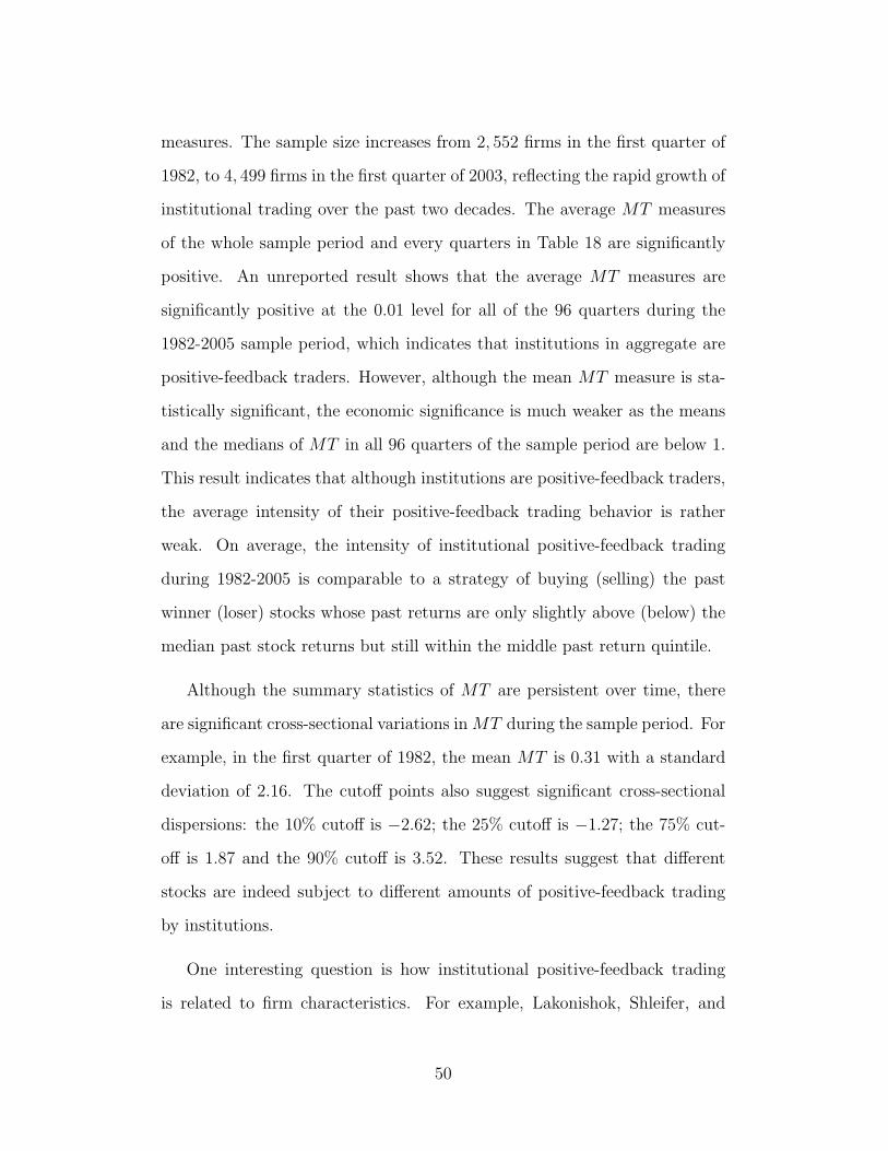
measures. The sample size increases from 2, 552 firms in the first quarter of

1982, to 4, 499 firms in the first quarter of 2003, reflecting the rapid growth of

institutional trading over the past two decades. The average MT measures

of the whole sample period and every quarters in Table 18 are significantly

positive. An unreported result shows that the average MT measures are

significantly positive at the 0.01 level for all of the 96 quarters during the

1982-2005 sample period, which indicates that institutions in aggregate are

positive-feedback traders. However, although the mean MT measure is sta-

tistically significant, the economic significance is much weaker as the means

and the medians of MT in all 96 quarters of the sample period are below 1.

This result indicates that although institutions are positive-feedback traders,

the average intensity of their positive-feedback trading behavior is rather

weak. On average, the intensity of institutional positive-feedback trading

during 1982-2005 is comparable to a strategy of buying (selling) the past

winner (loser) stocks whose past returns are only slightly above (below) the

median past stock returns but still within the middle past return quintile.

Although the summary statistics of MT are persistent over time, there

are significant cross-sectional variations in MT during the sample period. For

example, in the first quarter of 1982, the mean MT is 0.31 with a standard

deviation of 2.16. The cutoff points also suggest significant cross-sectional

dispersions: the 10% cutoff is −2.62; the 25% cutoff is −1.27; the 75% cut-

off is 1.87 and the 90% cutoff is 3.52. These results suggest that different

stocks are indeed subject to different amounts of positive-feedback trading

by institutions.

One interesting question is how institutional positive-feedback trading

is related to firm characteristics. For example, Lakonishok, Shleifer, and

50

Vishny (1992) observe stronger positive-feedback trading by pension funds

in small stocks. In addition, Grinblatt, Titman, and Wermers (1995) find

that positive-feedback trading by mutual funds is stronger on the buy side

than on the sell side, implying that winner stocks experiences more positive-

feedback trading than does losers.

In order to examine the relationships between institutional positive-feedback

trading and firm characteristics, I calculate for each month the average

firm characteristics of MT quintiles and report in table 19 the time-series

means and t-statistics of the cross-sectional averages. The firm characteris-

tics include monthly stock return, size, the book-to-market ratio (henceforth

BE/ME), turnover, analyst coverage, return volatility, and firm age. I ex-

amine these firm characteristics because they are documented to affect stock

return momentum. Firm size is the natural log of a firm’s market capital-

ization. BE/ME is the summation of book equity and deferred tax of a

firm divided by its market equity. I apply BE/ME calculated at the fiscal

year end of year t to the one-year period starting from July of year t + 1.

Turnover is the monthly trading volume divided by total shares outstand-

ing. Analyst coverage is the number of analysts providing a firm’s one year

earnings forecasts. Because trading volumes of NASDAQ stocks are inflated

relative to those of NYSE/AMEX stocks, I follow Chen, Hong, and Stein

(2002) to demean the turnovers with the cross sectional averages of NAS-

DAQ or NYSE/AMEX turnovers according to the stock market in which the

firms are listed.39 I also follow Griffin and Lemmon (2002) to adjust a firm’s

analyst coverage by the average coverage of the NYSE size quartile that the

firm belongs to.40 I calculate return volatility and firm age following Jiang,

39Unless otherwise specified, all the turnovers in this paper are demeaned turnovers.40Unless otherwise specified, all the analyst coverages in this paper are residual analyst

coverages. My results are not changed when I use another size-adjusted analyst coverage

51

Lee, and Zhang (2005) and Zhang (2006). In particular, for month t, return

volatility is the standard deviation of daily stock returns of 25 trading days

up to the end of month t-1. Age of a firm is the number of months from the

firm’s first CRSP monthly return record.

Table 19 presents three results on the relationships between institutional

positive-feedback trading and firm characteristics:

First, consistent with Lakonishok, Shleifer, and Vishny (1992), high MT

stocks are relatively small in size. The average firm size of the top MT quin-

tile is 19.96, lower than those of the middle three quintiles. In the meantime,

low MT stocks are also relatively small in size, with an average firm size

of 19.78. Second, there is no discernable difference in the levels of institu-

tional positive-feedback trading between winner stocks and loser stocks. For

example, the average monthly returns of the top MT quintile is 1.01%, not

significantly different from 1.17%, the average returns of the bottom MT

quintile. One possible reason of the difference between my finding and Grin-

blatt, Titman, and Wermers (1995) is that my sample includes all institutions

while their samples include only mutual funds. Third, the strength of insti-

tutional positive-feedback trading is related to turnover, BE/ME, analyst

coverage, return volatility and firm age. Table 19 shows that institutional

positive-feedback trading level increases in turnover and return volatility and

decreases in BE/ME, coverage and firm age. The differences in turnover,

BE/ME, analyst coverage, return volatility and firm age between the top

and the bottom MT quintiles are 0.12, 0.05, −0.79, 0.004 and −53, all sta-

tistically significantly at the standard level.

measure suggested by Hong, Lim, and Stein (2000).

52

2.2.2 Institutional Positive-Feedback Trading and Return Momen-

tum

This subsection examines the effect of institutional positive-feedback trading

on stock return momentum. I independently sort stocks into three groups

of MT and ten groups of past performance and then calculate, for each

MT groups, the momentum profits of the six-month formation/six-month

holding strategy following Jegadeesh and Titman (2001).41 In particular, at

the beginning of every month, I form two-dimensional portfolios on the MT

measures and the past six-month cumulative stock returns and hold these

portfolios for six months.

The result is reported in Table 20 Panel A, which shows that momentum

profits increase in the MT measures, ranging from 1.08% (t-stat 2.95) for

the bottom MT tercile to 1.61% (t-stat 4.72) for the top MT tercile. The

difference in momentum profits between the top and the bottom MT terciles

is 0.53% (t-stat 3.21), significant at the 0.01 level. The difference is not only

statistically significant but economically significant as well, compounding to

an annual return difference of 8.58%.

For a robustness check, I further report in Panel B the results of Fama-

French three-factor regressions of momentum profits. The difference in the

three-factor alphas between the top and bottom MT terciles is 0.48% (t-stat

3.02), close to the difference in momentum profits reported in Panel A. To

summarize, Table 20 presents strong empirical evidence that institutional

positive-feedback trading contributes to stock return momentum.

41I also repeat the tests in this paper with an alternative momentum strategy that skipsa month between formation and holding period. The results are not changed with theskip-a-month momentum strategy.

53

Trading cost is always a concern when we evaluate the profitability of

a trading strategy. If, for example, employing momentum strategy to high

MT stocks is associated with much higher transaction costs than to low MT

stocks, then the difference in transaction costs could offset the difference in

momentum profits. Although the data of transaction costs are not directly

available, we could evaluate the transaction costs based on firm characteris-

tics across MT levels. Specifically, if we consider size and turnover as proxies

for liquidity and hence trading cost, then the trading costs of applying mo-

mentum strategies to high MT stocks should be no higher than that of low

MT stocks because as shown in Table 19, high MT stocks are only slightly

smaller in firm size but much higher in turnover than low MT stocks.

2.2.3 Robustness Check with Firm Size, BE/ME and Turnover

Three most important firm characteristics, size, BE/ME and turnover, have

been documented to have considerable impact on return momentum. For

example, Hong, Lim, and Stein (2000) and Jegadeesh and Titman (2001) ob-

serve stronger return momentum in small stocks than in large stocks. Daniel

and Titman (1999) shows that return momentum is stronger in low BE/ME

stocks than in high BE/ME stocks. Lee and Swaminthan (2000) find that

return momentum is more prevalent for the stocks with higher turnover.

This subsection is intended to check whether the effect of institutional

positive-feedback trading on return momentum is robust after controlling for

size, BE/ME and turnover. In addition, it is also interesting to understand

the relationships between the effect of institutional positive-feedback trading

and those of size, BE/ME or turnover on return momentum.

I conduct the tests in this regard by calculating the profits of the six-

54

month formation and six-month holding momentum strategy for stock port-

folios two-dimensionally sorted on the MT measure and size, or BE/ME, or

turnover. In particular, at the beginning of month t, I independently sort

stocks into three groups of MT , three groups of size, BE/ME or turnover,

and five groups of past six-month cumulative returns.42 Then all these three-

dimensional portfolios are held for six months. This momentum strategy is

the same as in Jegadeesh and Titman (2001) except that I form five groups

of past returns instead of ten groups in order to ensure enough number of

stocks in each three-dimensional portfolio.

Panel A of Table 21 reports average monthly returns of the three-dimensional

portfolios sorted on size, MT and past return, while Panel B provide a com-

parison of the momentum profits (W-L) for the three by three size-MT

groups. Within all three size groups, momentum profits are increasing in

the MT measure. Specifically, the differences in monthly momentum profits

between high and low MT stocks are 0.45% (t-stat 2.73), 0.38% (t-stat 2.38)

and 0.44% (t-stat 2.22), all statistically significant at the standard levels. To

summarize, Table 21 shows that the effect of institutional positive-feedback

trading on return momentum persists after controlling for firm size.

One might attribute the result in Table 21 to the variation of size within

each size group. To address this concern, I report the average decile ranks

of size and MT for each size-MT group in Table 21 Panel A. In particular,

I first assign decile ranks of size and MT to the stocks in each cross-section,

where 1 is assigned to the bottom decile and 10 to the top decile. Next, I

calculate the time series-averages of the cross sectional means of size and MT

42Size is measured at the end of month t-1. I match BE/ME at the fiscal year end ofyear t-1 to the one-year period starting from July of year t+1. Turnover is the demeanedturnover of month t-1.

55

ranks for each size-MT group. As shown in Panel A, within each size group

the size-MT groups are almost undistinguishable in size but vastly different

in MT , indicating that the difference in momentum profits between the high

and low MT group is driven by the variation in MT rather than firm size.

In addition, Panel B shows that the effect of firm size on stock return

momentum is also robust after controlling for institutional positive-feedback

trading. For example, the differences in monthly profits between large and

small stocks across MT groups are 0.62% (t-stat 3.60), 0.35% (t-stat 1.89)

and 0.63% (t-stat 2.99), all statistically significant at the standard levels.

These results indicate that the effects of firm size and institutional positive-

feedback trading on return momentum are independent of each other.

Similarly, Table 22 examine the effect of institutional positive-feedback

trading on stock return momentum after controlling for BE/ME. Panel A

reports and Panel B compares the momentum profits across the MT-BM

groups. We can see in Panel B that within two of the three BE/ME groups,

the differences in momentum profits between high and low MT stocks are

economically and statistically significant. In particular, the differences in

monthly momentum profits between high and low MT stocks are 0.74% (t-

stat 4.00), 0.23% (t-stat 1.28) and 0.41% (t-stat 2.02). Although one of the

difference 0.23% is not statistically significant, the other difference 0.74% is

not only statistically significant at the 0.01 level but also much higher than

0.53%, the average effect of MT as shown in Table 20. Therefore, the results

of Table 22 verify that the effect of institutional positive-feedback trading is

robust to the control of BE/ME.

In order to address the concern that the result might be due to the varia-

tion of BE/ME within each BE/ME group, I also calculate the average decile

56

ranks of BE/ME and MT for each BM-MT portfolio. Specifically, I first as-

sign decile ranks of BE/ME and MT to the stocks in each cross-section,

where 1 is assigned to the bottom decile and 10 to the top decile. Next, I

calculate the time series averages of the cross sectional means of the ranks.

Panel A shows that within each BE/ME group, there is no discernable dif-

ference in BE/ME but vast difference in MT between the BM-MT groups,

indicating that the differences in momentum profits between high and low

MT groups are caused by the variation of institutional momentum trading

rather than BE/ME.

In addition, Table 22 Panel B shows that the effect of BE/ME on stock

return momentum is also robust after controlling for institutional positive-

feedback trading. For example, the differences in monthly momentum profits

between the low BE/ME and the high BE/ME stocks for the three MT

groups are 0.19% (t-stat 0.93), 0.54% (t-stat 2.54) and 0.51% (t-stat 2.22),

respectively.

Last, Table 23 presents the robustness check which controls of turnover.

Panel A reports the average monthly returns of each three-dimensional port-

folios sorted on turnover, MT , and past return, while Panel B presents the

momentum profits across turnover-MT groups. We can see that within all

three turnover groups, momentum profits are increasing with MT level and

the differences in momentum profits between high and low MT stocks are

statistically significant two out of the three turnover groups. In particu-

lar, the differences in monthly momentum profits between high and low MT

stocks are 0.12% (t-stat 0.78), 0.32% (t-stat 2.38) and 0.59% (t-stat 3.57).

To summarize, Table 23 shows that the contribution of institutional positive-

feedback trading to stock return momentum persists after controlling for

57

turnover.

I also report in Panel A the average decile ranks of turnover and MT for

each turnover-MT portfolio, which show that within each turnover group,

the turnover-MT groups are almost undistinguishable in turnover but vastly

different in MT . This result indicates that the difference in momentum

profits between high and low MT groups is driven by institutional positive-

feedback trading rather than turnover. Panel B shows the coexistence of

the effects of turnover and institutional positive-feedback trading on stock

return momentum. For example, the difference in monthly profits between

high turnover and low turnover stocks are 0.31% (t-stat 1.64), 0.51% (t-

stat 2.85) and 0.77% (t-stat 3.87), all statistically significant at the standard

levels.

2.2.4 Robustness Check With The Residual MT Measures

One might argue that the sub-portfolio analysis based on three-dimensional

sorts in Table 21 to Table 23 is incomplete in the sense that they control for

size, BE/ME and turnover separately, and that the effect of the MT measure

could be altered if these factors are controlled simultaneously. An ideal test

to address this concern is to sort stocks independently on size, BE/ME,

turnover, and MT, and then examine momentum profits across this multi-

dimensionally sorted portfolios. However, this method will require a huge

sample size. For example, if in each cross-section we sort stocks into three

groups based on each of the aforementioned four variables and five groups

based on past returns, in total 405 sub-portfolios will be generated, leaving

very few or even no stocks in some portfolios given the current sample size.

In order to control for size, BE/ME and turnover simultaneously, I create

58

a residual MT measure, ResMT1. The methodology is similar to Hong,

Lim, and Stein (2000) in a different context. Specifically, in each month t of

the sample period, I estimate a cross-sectional regression of the MT measure

on firm size, BE/ME, and demeaned turnover of month t-1. I then take

the residuals from these regressions as the ResMT1 measures, which is the

component of MT measures that is orthogonal to size, BE/ME and turnover.

Next, I repeat the test of Table 20 but with the ResMT1 measure rather

than the original MT measure. In particular, at the beginning of every

month, I form three by ten two-dimensional portfolios independently on the

ResMT1 measures and the past six-month cumulative stock returns and hold

these portfolios for six months.

The result is reported in Table 24 Panel A, which shows that momentum

profits increase in the ResMT1 measures, ranging from 0.93% (t-stat 2.42)

for the bottom ResMT1 tercile to 1.50% (t-stat 4.17) for the top ResMT1

tercile. The difference in momentum profits between the top and the bottom

ResMT1 terciles is 0.57% (t-stat 3.24), significant at the 0.01 level. Panel B

further report the Fama-French three-factor alphas for momentum profits of

the three ResMT1 groups. The difference in the three-factor alphas between

the top and bottom ResMT1 terciles is 0.48% (t-stat 2.87). To summarize,

Table 24 shows that the effect the MT measure on return momentum is

robust when we control for size, BE/ME and turnover simultaneously.

Besides size, BE/ME and turnover, three other firm characteristics were

also found to affect return momentum. Specifically, Hong, Lim, and Stein

(2000) shows that return momentum is stronger in stocks with lower analyst

coverage. Jiang, Lee, and Zhang (2005) and Zhang (2006) document stronger

momentum in firms with higher return volatility and shorter history. In order

59

to further control for analyst coverage, return volatility and firm age, I create

a second residual MT measure, ResMT2. In particular, in each month t of

the sample period, I estimate a cross sectional regression of the MT measure

on firm size, BE/ME, demeaned turnover, residual analyst coverage of month

t-1, return volatility in the 25 trading days up to the end of month t-1, and

firm age of month t-1.43 The ResMT2 measures are the residuals from these

regressions.

Next, I repeat the test in Table 24 with the ResMT2 measure rather than

the ResMT1 measure. In particular, I form three by ten two-dimensional

portfolios independently on the ResMT2 measures and the past six-month

cumulative stock returns and hold these portfolios for six months. Table 25

Panel A shows that momentum profits increase in the ResMT2 measures,

ranging from 0.96% (t-stat 2.52) for the bottom ResMT2 tercile to 1.45% (t-

stat 4.02) for the top ResMT2 tercile. The difference in momentum profits

between the top and the bottom ResMT2 quintile is 0.49% (t-stat 2.89),

significant at the 0.01 level. Panel B further shows that the difference in the

three-factor alphas between the top and bottom ResMT2 terciles is 0.42%

(t-stat 2.52). These results suggest that the effect of the MT measure persists

after further controlling for analyst coverage, return volatility and firm age.

2.2.5 Robustness Check with An Alternative Measure of Positive-

Feedback Trading

In this subsection I further examine the robustness of the effect of institu-

tional positive-feedback trading with an alternative positive-feedback trading

measure. In particular, in equation (1) that describes the estimation of the

43The estimation of return volatility and firm age is the same as in Jiang, Lee, andZhang (2005), and Zhang (2005).

60

MT measure, I adjusted quarterly institutional trading, 4holdit, by total

institutional trading during the estimation period,∑8

t=1 |4holdit|. Since the

adjusted quarterly institutional trading 4holdit∑8

t=1|4holdit|

add up to 1 across the

eight quarters during estimation period, MT measure ranges between -5 and

5. This nice property of the MT measure enable us to easily assess the

intensity of institutional positive-feedback trading by the value of the MT

measure. For example, a MT measure of 4 indicates that the intensity of

institutional positive-feedback trading is comparable to a strategy of buy-

ing past winners in the second highest past return decile (ppindex equals 4)

and/or sell past losers in the second lowest past return decile (ppindex equals

-4).

While the aforementioned adjustment of total institutional trading make

the MT measure easily interpreted, it results in a disadvantage that the MT

measure does not capture the magnitude of total institutional trading. For

example, suppose institutions are positive-feedback traders to both stock i

and stock j. Suppose further that institutions trade both stocks twice during

the two-year estimation period. In particular, they buy 1% of stock i’s total

shares outstanding in quarter 3 when it is an extreme past winner (ppindexi3

equals 5) and sell 1% of stock i in quarter 7 when it is an extreme past loser

(ppindexi7 equals −5). In addition, institutions buy 2% of stock j’s shares in

quarter 3 when it is an extreme past winner and sell 2% of stock j in quarter

7 when it is an extreme past loser. Then for stock i, the product terms

4holdit∑8

t=1|4holdit|

ppindexit are 2.5 (0.5 times 5) for quarter 3 and 7 but zero for

the rest of the quarters, resulting in a MT measure of 5 for stock i. Stock j’s

product terms 4holdjt∑8

t=1|4holdjt|

ppindexjt are also 2.5 (0.5 times 5) for quarter 3

and 7 but zero for the rest of the quarters, leading to a MT measure of 5 for

stock j. Although the MT measures of stock i and j are both 5, institutional

61

positive-feedback trading could have stronger impact on stock j than stock

i because institutions trade stock j in bigger volume than they trade stock

i. In order to address this concern, I construct an alternative measure of

institutional positive-feedback trading, the MTWO measure (MT measure

without adjustment), following the equation below.

MTWOi =8∑

t=1

(4holdit × ppindexit) (6)

The MTWO measure is constructed with the same method as the MT

measure except that I do not adjust quarterly institutional trading, 4holdit,

with total institutional trading during the estimation period,∑8

t=1 |4holdit|.As a result, the MTWO measures captures the magnitudes of institutional

trading.

I calculated the MTWO measure following equation (2) and examine

its correlation with the MT measure. The Spearman rank correlation is as

high as 0.87, indicating that the MTWO measure and the MT measure are

strongly correlated. Next, I repeat the test in Table 20 but with the MTWO

measure rather than the original MT measure. The result is reported in

Table 26 Panel A, where momentum profits increase from 1.06% per month

(t-stat 2.93) for the bottom MTWO tercile to 1.55% per month (t-stat 4.57)

for the top MTWO tercile. The difference in momentum profits between the

top and the bottom MTWO terciles is 0.49% (t-stat 2.94), significant at the

0.01 level. Panel B further report the Fama-French three-factor alphas for

momentum profits of the three MTWO groups. The difference in the three-

factor alphas between the top and bottom ResMT1 terciles is 0.45% (t-stat

2.76). To summarize, Table 26 shows that the effect institutional positive-

feedback trading on return momentum is robust with the alternative measure

62

that considers the magnitudes of institutional trading.

2.3 Institutional Positive-Feedback Trading and Stock

Price Efficiency

This section aims at investigating the effect of institutional positive-feedback

trading on stock price efficiency. Theoretically it is not clear whether or not

institutional positive-feedback trading improves the market efficiency. On

one hand, institutional positive-feedback trading could improve market effi-

ciency if it speeds up the correction of stock mispricing. Specifically, if market

underreact to positive (negative) news and thus underprice (overprice) the

past winners (losers), then institutional positive-feedback trading can speed

up the price adjustment process by pushing the winners (losers) further to

the ‘correct’ level. On the other hand, institutional positive-feedback trad-

ing could deteriorate market efficiency by driving stock prices further away

from their fundamentals if such trading is unrelated to information on firm

fundamentals or is induced by overreaction.

2.3.1 Evidence from Earnings Revision

Perhaps the most important information regarding stock prices is earnings

information. Chan, Jegadeesh, and Lakonishok (1996) observe the coex-

istence of return momentum and earnings momentum, namely, both past

stock return and past accounting performance predict future stock returns.

They examine revisions of earnings analyst forecasts across past return levels

during the one-year post-ranking period, and find that post-ranking earnings

revisions are more favorable for past winners than for past losers. An inter-

63

national study by Hong, Lee, and Swaminathan (2003) studies eleven equity

markets and find that stock return momentum only exists in the markets

where earnings momentum is profitable, indicating that stock return mo-

mentum and earnings momentum share the same information dissemination

system.

Post-ranking earnings revision provides us with an ideal test vehicle not

only because earnings revision has implication on stock mispricing but also

because earnings revision, unlike stock return, is exogenous to institutional

trading. Under the hypothesis that institutional positive-feedback trading

improves the market efficiency, high MT past winners (losers) are more un-

derpriced (overpriced) than low MT past winners (losers), and institutional

positive-feedback trading helps adjust stock prices to their ’correct’ levels by

creating stronger momentum in high MT stocks. Therefore, in this case we

expect to observe that by positive-feedback trading, institutions buy (sell)

the past winners (losers) that will experience more favorable (unfavorable)

earnings revision during the post-ranking period than other past winners

(losers). As a result, if institutional positive-feedback trading improves the

market efficiency, we would expect the biggest difference in post-ranking

earnings revision between past winners and past losers to appear in the top

MT quintile. In other words, in this scenario the bigger return difference

between high MT past winners and past losers should be justified by the

stronger market underreaction and hence bigger difference in post-ranking

earnings revision.

Following Chan, Jegadeesh, and Lakonishok (1996) and Hong, Lee, and

Swaminathan (2003), I use the average one-year earnings forecasts in this

64

study and calculate earnings revision following the formula below.

ERit =(EFit − EFit−1)

Pit−1

(7)

Where ERit is earnings revision of firm i from month t− 1 to month t; EFit

and EFit−1 are the mean earnings forecasts of firm i in month t and t − 1,

respectively; Pit−1 is the stock price of firm i at the end of month t−1. ERit

is positive if analysts on average raise the earnings forecasts of firm i from

month t− 1 to month t and negative if they adjust the forecasts downwards.

One issue of equation (3) is that the mean forecasts before and after an

announcement date cover different fiscal years. To address this issue, when a

firm announces earning in month t, I treat earnings revision around month t

following Hong, Lee, and Swaminathan (2003): if the earnings announcement

date is before the I/B/E/S summary date, then earnings revision of month t is

calculated as the difference between mean one-year earnings forecast of month

t and mean two-year earnings forecast of month t−1 divided by the stock price

at the end of month t− 1. On the other hand, if the earnings announcement

date is after the I/B/E/S summary date, then earnings revision of month t

is still calculated following equation (3) but earnings revision of month t + 1

is calculated as the difference between mean one-year earnings forecast of

month t + 1 and mean two-year forecast of month t divided by the stock

price at the end of month t.

I begin by sorting stocks independently into quintiles of MT and past

six-month returns and examine the average earnings revisions during the

one-year period after portfolio formation. In particular, at the beginning

of month t, I independently sort stocks into quintiles of the MT measures

as well as cumulative returns in the past six months. Next, I examine the

65

average earnings revisions for each month in the one-year period starting

from t and report the results in Panel A of Table 27.

Consistent with Chan, Jegadeesh, and Lakonishok (1996), most of the

mean earnings revisions are negative, revealing the fact that initially over-

optimistic analysts gradually adjust their forecasts downwards to the ‘correct’

level. Moreover, within each MT quintile, earnings revisions are more favor-

able for winner stocks than for loser stocks in every of the twelve months

after portfolio formation, indicating market underreaction.

In order to examine whether institutional positive-feedback trading im-

proves market efficiency, I compare the differences in earnings revisions be-

tween winners and losers for the top and bottom MT quintiles and report

the results in Panel B. Table 27 Panel B shows that in five out of the twelve

months, the differences in earnings revisions between winners and losers are

actually smaller in the top MT quintile than in the bottom MT quintile.

Although the other seven of the twelve differences are positive, none of them

is significant at the standard levels.

Table 27 reveals that the stronger momentum generated by institutional

positive-feedback trading is not accompanied by the bigger difference in the

post-ranking earnings revision between winners and losers. Therefore, the

evidence from earnings revision is inconsistent with the hypothesis that in-

stitutional positive-feedback trading improves market efficiency.

2.3.2 Evidence from Long-Term Reversal of Momentum Profits

Extant research has observed that momentum profit reverts one year after

portfolio formation, which suggests that return momentum results from mis-

66

pricing instead of risk.44 When the prices of winners and losers start to

converge back to the levels that correctly reflect firm fundamentals, momen-

tum profit reverts.

Interestingly, the model of Hong and Stein (1999) predicts that stocks that

attract more positive-feedback trading will experience deeper long-term re-

versal in momentum profits. This occurs in their model because the positive-

feedback traders push the past winners further up and beat the past losers

further down, thereby driving stock prices even further away from their fun-

damentals. This claim is consistent with the hypothesis that institutional

positive-feedback trading hampers market efficiency. If, on the contrary, in-

stitutional positive-feedback trading improves market efficiency and drives

the prices of underpriced (overpriced) winners (losers) further to their funda-

mental values, then we would expect no difference in the long-term reversals

of momentum profits for the stocks that experience different amount of in-

stitutional positive-feedback trading.

In order to examine the long-term reversals across different levels of in-

stitutional positive-feedback trading, I sort stocks into MT quintiles and ex-

amine the magnitudes of long term reversals in their momentum profits. In

particular, at the beginning of month t, I form five by five portfolios indepen-

dently on the MT measure and past six-month stock returns, and calculate

cumulative momentum profits (winners minus losers) for each MT quintile

up to each month in the three-year period from month t.

Table 28 reports the results. First, consistent with previous studies,

within each MT quintile the cumulative momentum profits peak in the

twelfth month after portfolio formation and then slowly drift downwards.

44See, for example, Jegadeesh and Titman (2001) for the analysis of long term reversalin momentum profit.

67

The right most column reports the change in cumulative momentum prof-

its from the twelfth month to the thirty-sixth month. All the changes are

negative, reflecting long-term reversals in momentum profits.

Second, the pattern of long term reversals across different MT levels is

evident: the magnitudes of the reversals are increasing with MT level, from

−3.44% of the bottom MT quintile to −6.36% of the top MT quintile. This

result indicates that stocks that receive more institutional positive-feedback

trading experience much stronger reversals in momentum profits than stocks

lack of institutional positive-feedback trading.

In order to provide a clear view of this pattern, I plot long-term cu-

mulative momentum profits of the top and bottom MT quintile during the

three-year post-formation period. Figure 2 shows very clearly that the top

MT quintile exhibits much deeper reversal than the bottom MT quintile: al-

though returns of the top MT quintile reaches a much higher peak than that

of the bottom MT quintile, the two return sequences reach approximately

the same low levels three years after portfolio formation.

To summarize, this subsection shows that stocks subject to stronger in-

stitutional positive-feedback trading exhibit much deeper long-term reversal

in momentum profits during the three-year post-ranking period. This re-

sult is consistent with hypothesis that institutional positive-feedback trading

hampers market efficiency.

2.3.3 The Relationship Between MT and FIT Measures

Chapter one presents evidence that higher fraction of institutional trading

volume leads to greater price efficiency and therefore lower momentum. This

68

result suggests that institutions act as rational traders in generals. Chapter

two shows that although institutions are in general rational traders, their

particular trading behaviors could still hamper price efficiency. For exam-

ple, when institutional act as positive-feedback traders, their trend-chasing

behavior intensifies momentum and therefore hampers price efficiency. Since

both the MT measure and the FIT measure affect the magnitudes of mo-

mentum, I examine the relationship of these two measures.

First, I calculate the correlation between the FIT measure and the MT

measure, which is as low as 0.005, indicating that the two measures are

not correlated. This results show that stocks with higher fraction of insti-

tutional trading volume are not the stocks subject to stronger institutional

positive-feedback trading. This result is consistent with the discussion in the

dissertation that the effect of positive-feedback trading on momentum is not

necessarily the evidence that institutions overall hamper price efficiency be-

cause positive-feedback trading is only one of the many institutional trading

strategies.

Second, I calculate the momentum profits across the stocks two-dimensionally

sorted on the FIT measure and the MT measure. In particular, At the be-

ginning of month t, I independently sort stocks into three groups of the MT

measures, three groups of one-quarter lag FIT measures, and quintiles of

cumulative returns over the six-month period up to the end of month t-1.

Following the six-month holding/six-month formation strategy of Jegadeesh

and Titman (2001), I hold these three-dimensionally sorted portfolios for six

months.

Table 29 Panel A reports the average monthly returns of the portfolios

and Panel B reports the comparisons of momentum profits across the FIT-

69

MT groups. The results show that the effects of the FIT measure and the

MT measure on stock return momentum are independent of each other.

70

3 Conclusion

My dissertation studies the the effects of institutional trading on stock price

efficiency. I find that institutional trading has significant yet complicated

impact on price efficiency. In particular, institutional trading in general

improves price efficiency. For example, major stock market anomalies such

as stock return momentum, post earnings announcement drift, and the book-

to-market effect are much stronger in stocks with lower institutional trading

volume. However, some institutional trading behaviors could hamper stock

price efficiency even though institutions are generally rational arbitrageurs.

Specifically, I show that when institutions act as positive-feedback traders,

their trading contributes to stock return momentum and hampers prices

efficiency.

71

Figures

Figure 1: Fitted Distributions of Earnings-Announcement Returns AcrossFIT Levels

This table presents the fitted distributions of the four-day returns aroundearnings-announcements across FIT levels. I calculate the four-day marketmodel adjusted abnormal returns around quarterly earnings announcementsfor the sample firms. Then for each month, I sort firms with quarterlyearnings-announcements in that month into deciles of one-quarter lag FIT.I then pool the earnings-announcement returns for each FIT decile, fit thesereturns into normal distribution, and plot the distributions across the FITdeciles. FitRank1 represents the bottom FIT decile, FitRank4 representsthe 4th FIT decile, FitRank7 represents the 7th FIT decile, and FitRank10represents the top FIT decile.

72

Figure 2: Construction of the MT Measure

This figure illustrates the first three steps of constructing the MT measure.There are in total eight quarters in the estimation period. I first calculateinstitutional trading in each of the eight quarters and then sum up the absolutevalue of the quarterly trading as shown in Panel A. Next, for each quarter ofthe two-year estimation period, I calculate past performance index (PPindex)and weight of the trading as shown in Panel B.

Panel A: Step One

Panel B: Step Two and Three

73

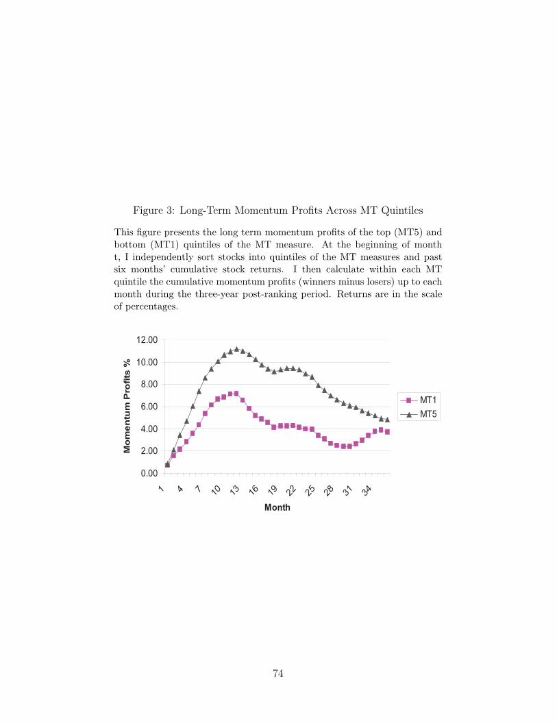
Figure 3: Long-Term Momentum Profits Across MT Quintiles

This figure presents the long term momentum profits of the top (MT5) andbottom (MT1) quintiles of the MT measure. At the beginning of montht, I independently sort stocks into quintiles of the MT measures and pastsix months’ cumulative stock returns. I then calculate within each MTquintile the cumulative momentum profits (winners minus losers) up to eachmonth during the three-year post-ranking period. Returns are in the scaleof percentages.

0.00

2.00

4.00

6.00

8.00

10.00

12.00

1 4 710

13

16

19

22

25

28

31

34

Month

Mo

me

ntu

m P

ro

fits

%

MT1

MT5

74

Tables

Table 1: Summary Statistics

This table summarizes FIT, FIB, FIS as well as firm characteristics of the sample, which con-tains 236,908 firm-quarters during 1980 to 2005. FIT, FIB and FIS are calculated followingequations (1) to (6) in the paper. Betas of individual stocks are obtained from CRSP; Sizeis the natural log of a firm’s market capitalization; BM/ME is calculated as the summationof a firm’s book equity and deferred tax divided by the firm’s market equity; past return isthe cumulative return of a firm during the past six months. The residual analyst coverageis calculated following Griffin and Lemmon (2002) by subtracting the average analyst cov-erage of the NYSE size quartile of a firm from the firm’s analyst coverage. Turnover is thetotal quarterly turnover calculated as the summation of the monthly turnovers during thequarter, where monthly turnover is obtained by dividing the total trading volume of a firmby its total shares outstanding. Idiosyncratic volatility is the monthly updated volatilityof residuals from the Fama-French 3 factor regression for the previous five-year estimationperiod. Dividend yield is the dividend payment of a firm in the previous fiscal year dividedby its share price. Illiquid is the annual illiquidity measure (multiplied by 10.000) calculatedfollowing Amihud (2002).

Variables Mean StDev P10 P25 Median P75 P90FIT 0.54 0.41 0.04 0.23 0.49 0.75 1.03FIB 0.28 0.23 0.01 0.10 0.24 0.39 0.56FIS 0.25 0.21 0.01 0.07 0.21 0.35 0.51

Institutional Ownership 0.37 0.27 0.01 0.13 0.35 0.57 0.74Quarterly Turnover 0.22 0.23 0.04 0.08 0.15 0.27 0.46

Beta 0.82 0.56 0.15 0.41 0.77 1.15 1.55Ln(ME) 20.03 1.58 18.14 18.81 19.85 21.02 22.18

BM 0.73 0.53 0.23 0.39 0.63 0.95 1.34Ret(-6,-1) 0.10 0.33 -0.20 -0.06 0.07 0.21 0.42

Residual Analyst Coverage -0.03 5.32 -5.33 -2.69 -0.52 2.45 6.33Stock Price 40.23 883.24 9.13 13.63 21.75 34.00 50.25

Idiosyncratic Volatility 0.09 0.04 0.05 0.07 0.08 0.11 0.14Dividend 0.03 0.09 0.00 0.00 0.02 0.05 0.08

Illiq 2.16 2.61 0.29 0.59 1.30 2.73 5.06

75

Table 2: Firm Characteristics Across FIT Levels

This table reports firms characteristics across FIT quintiles. Time-series means and t-statistics ofthe cross-sectional averages are reported. Betas of individual stocks are obtained from CRSP; Sizeis the natural log of a firm’s market capitalization; BM/ME is calculated the summation of a firm’sbook equity and deferred tax divided by the firm’s market equity; past return is the cumulativereturn of a firm during the past six months. The residual analyst coverage is calculated followingGriffin and Lemmon (2002) by subtracting the average analyst coverage of the NYSE size quartileof a firm from the firm’s analyst coverage. Turnover is the total quarterly turnover calculated asthe summation of the monthly turnovers during the quarter, where monthly turnover is obtained bydividing the total trading volume of a firm by its total shares outstanding. Idiosyncratic volatility isthe monthly updated volatility of residuals from a Fama-French 3 factor regression for the previousfive-year estimation period. Dividend yield is the dividend payment of a firm in the previous fiscalyear divided by its share price. Illiquid is the annual illiquidity measure calculated following Amihud(2002). Since Illiquidity levels vary over time with total market volumes, I transfer the illiquiditymeasures into standardized ranks between 0 and 1 following Chan, Jegadeesh, and Lakonishok(1996).

Variables Low FIT 2 3 4 High FIT High-Low t-statFIB 0.03 0.16 0.26 0.36 0.56 0.53 94.92FIS 0.03 0.14 0.24 0.33 0.51 0.48 82.18

Institutional Ownership 0.06 0.30 0.43 0.49 0.48 0.42 48.07Quarterly Turnover 0.20 0.29 0.23 0.19 0.14 -0.06 -23.47

Beta 0.62 0.88 0.93 0.92 0.79 0.17 10.90Ln(ME) 18.96 19.76 20.45 20.54 20.12 1.16 38.54

BM 0.73 0.75 0.74 0.73 0.75 0.01 1.30Ret(-6,-1) 0.10 0.12 0.10 0.10 0.09 -0.01 -1.38

Residual Analyst Coverage -1.62 0.34 1.25 0.75 -0.70 0.92 12.00Stock Price 20.04 26.03 31.47 35.58 81.62 61.58 10.09

Idiosyncratic Volatility 0.09 0.10 0.09 0.09 0.09 0.00 -1.28Dividend 0.05 0.03 0.03 0.03 0.03 -0.02 -13.88

SP500Dummy 0.02 0.15 0.31 0.33 0.19 0.18 16.41Illiq 0.65 0.52 0.42 0.40 0.53 -0.19 -12.37

76

Tab

le3:

Cor

rela

tion

s

this

tabl

ere

port

sth

eco

rrel

atio

nco

effici

ents

ofth

elis

ted

vari

able

s.F

IT

,FIB

and

FIS

are

mea

sure

din

quar

ter

t,an

dF

IT

t−1

ism

easu

red

inqu

arte

rt-

1.IO

t−1,i

nsti

tuti

onal

owne

rshi

p,is

mea

sure

dat

the

end

ofqu

arte

rt-

1.B

eta

ises

tim

ated

usin

gth

eda

ilyre

turn

sin

the

prev

ious

cale

ndar

year

.L

n(M

E)

isth

ena

tura

llo

gof

mar

ket

capi

taliz

atio

nm

easu

red

atth

een

dof

quar

ter

t-1.

Ln(B

M)

BE

/ME

isca

lcul

ated

acco

rdin

gto

Fam

aan

dFr

ench

(199

2).

Ret

6is

retu

rns

ofth

esi

x-m

onth

peri

odup

toth

een

dof

quar

ter

t-1.

Prc

isth

est

ock

pric

eat

the

end

ofqu

arte

rt-

1.R

esA

Cis

the

resi

dual

anal

yst

cove

rage

atth

een

dof

quar

ter

t-1

calc

ulat

edfo

llow

ing

Gri

ffin

and

Lem

mon

(200

2).

S&

P50

0is

adu

mm

yva

riab

lew

hich

equa

ls1

ifat

the

begi

nnin

gof

quar

ter

tth

efir

mis

part

ofS&

P50

0co

mpo

site

inde

x.V

olty

isfir

mle

veli

deos

yncr

atic

vola

tilit

yof

CA

PM

esti

mat

edev

ery

year

follo

win

ga

five-

year

rolli

ngw

indo

wpr

oces

s.D

ivis

the

divi

dend

yiel

dob

tain

edby

divi

ding

afir

m’s

divi

dend

paym

ent

per

shar

eby

its

shar

epr

ice.

Illiq

isA

mih

ud(2

002)

’sill

iqui

dity

mea

sure

esti

mat

edin

the

prev

ious

cale

ndar

year

.

Mod

els

FIT

FIB

FIS

FIT

t−1

IO

t−1

Bet

aL

n(M

E)

Ln(B

M)

Ret

6P

rcR

esA

CS

P50

0V

olty

Div

Illiq

FIT

1.00

FIB

0.84

1.00

FIS

0.82

0.46

1.00

FIT

t−1

0.68

0.59

0.62

1.00

IO

t−1

0.48

0.41

0.50

0.49

1.00

Bet

a0.

040.

040.

070.

040.

301.

00L

n(M

E)

0.23

0.21

0.25

0.24

0.46

0.25

1.00

Ln(B

M)

0.07

0.06

0.04

0.06

-0.0

2-0

.19

-0.1

51.

00R

et6

-0.0

10.

01-0

.03

-0.0

30.

00-0

.02

0.03

0.06

1.00

Prc

0.09

0.07

0.08

0.08

0.08

0.00

0.17

-0.0

20.

041.

00R

esA

C0.

000.

010.

020.

000.

280.

160.

13-0

.03

-0.0

9-0

.05

1.00

SP

500

0.12

0.11

0.13

0.12

0.40

0.19

0.65

-0.0

3-0

.03

0.08

0.26

1.00

Vol

ty-0

.09

-0.0

7-0

.08

-0.1

00.

000.

35-0

.22

-0.1

50.

13-0

.07

0.09

-0.1

51.

00D

iv-0

.12

-0.1

2-0

.12

-0.1

2-0

.21

-0.3

0-0

.04

0.20

-0.0

1-0

.02

-0.0

9-0

.01

-0.3

51.

00Illiq

-0.0

8-0

.07

-0.1

2-0

.09

-0.4

8-0

.30

-0.8

60.

150.

11-0

.12

-0.2

0-0

.61

0.20

0.00

1.00

77

Table 4: Quarterly Fama-Macbeth Regressions: Determinants of TraderComposition

This table presents quarterly Fama-Macbeth regressions of FIT (M1-M4), FIB (M5-M6) and FIS (M7-M8). FITt−1, FIBt−1, and FISt−1 are one quarter lags. IOt−1 is institutional ownership at the endof quarter t-1. Beta is estimated using the daily returns in the previous calendar year. Ln(ME)t−1

is the natural log of market capitalization at the end of quarter t-1. Ln(BM) is BE/ME. Ret6 issix-month return up quarter t-1. Prct−1 is stock price at the end of quarter t-1. ResAC is residualanalyst coverage at the end of quarter t-1. S&P500 is a dummy variable which equals 1 if the firm ispart of S&P500 composite index. V olatility is CAPM ideosyncratic volatility. Dividend is dividendyield. illiq is Amihud (2002)’s illiquidity measure. Average Adj. R-square is the time series averages.In order to facilitate the estimation of economic significance, I follow Chan, Jegadeesh and Lakonishok(1996) to transform the independent variables into standardized ranks between 0 and 1. t-statisticsare calculated based on Newey-West standard errors.

FIT Regressions FIB Regressions FIS RegressionsModels M1 M2 M3 M4 M5 M6 M7 M8FITt−1 0.9337 0.7627 0.8879t-stat (31.13) (23.94) (16.56)FIBt−1 0.2612 0.2863 0.2364 0.2670t-stat (34.35) (27.12) (22.88) (15.96)FISt−1 0.2120 0.2429 0.1646 0.1979t-stat (17.44) (13.90) (22.55) (15.87)IOt−1 0.2323 0.6742 0.2341 0.0406 0.0416 0.1557 0.1570t-stat (7.00) (23.07) (7.16) (3.11) (3.30) (8.03) (8.30)Beta -0.0547 -0.1000 -0.0561 -0.0215 -0.0222 -0.0243 -0.0251t-stat (-8.41) (-8.29) (-8.54) (-6.62) (-6.79) (-8.23) (-8.55)Ln(ME)t−1 0.0261 0.1016 0.0235 0.0012 0.0008 0.0181 0.0173t-stat (1.70) (4.80) (1.66) (0.14) (0.09) (4.20) (4.37)Ln(BM) 0.0240 0.0497 0.0238 0.0156 0.0157 0.0013 0.0012t-stat (2.83) (2.87) (2.76) (3.69) (3.64) (0.27) (0.26)Ret6 -0.0188 -0.0716 -0.0188 0.0089 0.0087 -0.0274 -0.0277t-stat (-2.87) (-6.58) (-2.90) (1.87) (1.81) (-8.05) (-8.42)Prct−1 -0.0271 -0.1033 -0.0268 -0.0045 -0.0045 -0.0182 -0.0185t-stat (-1.16) (-2.16) (-1.14) (-0.37) (-0.37) (-2.02) (-2.02)ResAC -0.0772 -0.1480 0.0628 -0.0265 0.0368 -0.0404 0.0314t-stat (-18.63) (-13.12) (1.96) (-9.18) (2.27) (-19.39) (1.61)S&P500 -0.0783 -0.1577 -0.0769 -0.0293 -0.0293 -0.0393 -0.0394t-stat (-12.62) (-9.78) (-12.37) (-11.60) (-11.70) (-11.51) (-11.54)V olatility -0.1046 -0.2569 -0.1003 -0.0545 -0.0528 -0.0409 -0.0392t-stat (-15.30) (-12.81) (-14.73) (-13.34) (-12.52) (-11.69) (-11.51)Dividend -0.0731 -0.1423 -0.0737 -0.0468 -0.0474 -0.0148 -0.0153t-stat (-8.20) (-7.52) (-7.60) (-8.59) (-8.18) (-4.92) (-4.44)Illiq 0.1381 0.2625 0.1360 0.0566 0.0557 0.0578 0.0568t-stat (10.42) (8.88) (10.86) (9.16) (9.44) (8.10) (8.36)ResAC ∗ FIT -0.2424t-stat (-4.12)ResAC ∗ FIB -0.0486 -0.0598t-stat (-2.46) (-2.83)ResAC ∗ FIS -0.0606 -0.0641t-stat (-3.84) (-3.98)

Adj. R-sq 0.4180 0.4583 0.2369 0.4688 0.3614 0.3646 0.4030 0.407178

Tab

le5:

Per

sist

ence

inTra

der

Com

pos

itio

n:

Sub-P

ortf

olio

Anal

ysi

s

Pan

elA

repo

rts

the

aver

age

FIT

acro

ssla

gFIT

deci

les.

Pan

elB

repo

rts

the

aver

age

FIS

acro

ssla

gFIB

deci

les,

and

Pan

elC

repo

rts

the

aver

age

FIS

acro

ssla

gFIS

deci

les.

Eac

hqu

arte

r,I

sort

stoc

ksin

tode

cile

sac

cord

ing

toth

eir

one

quar

ter

lag

FIT

(Pan

elA

),or

lag

FIB

(Pan

elB

),or

lag

FIS

(Pan

elC

),an

dca

lcul

ate

aver

age

FIT

,or

FIB

,or

FIS

for

each

deci

le.

Ith

enca

lcul

ate

the

tim

ese

ries

mea

nsan

dt-

stat

isti

csof

the

cros

s-se

ctio

nalav

erag

esfo

rea

ch.

Low

Hig

h1

23

45

67

89

10H

igh-

Low

t-va

lue

Pan

elA

:FIT

Acr

oss

Dec

iles

ofO

neQ

uart

erLag

FIT

FIT

(%)

0.08

0.17

0.32

0.43

0.52

0.60

0.67

0.75

0.84

1.02

0.94

(77.

07)

Lag

FIT

(%)

0.02

0.09

0.23

0.35

0.45

0.55

0.64

0.75

0.90

1.40

1.38

Pan

elB

:FIB

Acr

oss

Dec

iles

ofO

neQ

uart

erLag

FIB

FIB

(%)

0.06

0.09

0.17

0.23

0.27

0.31

0.34

0.38

0.42

0.47

0.41

(66.

26)

Lag

FIB

(%)

0.00

0.04

0.10

0.16

0.22

0.27

0.33

0.40

0.49

0.76

0.75

Pan

elC

:FIS

Acr

oss

Dec

iles

ofO

neQ

uart

erLag

FIS

FIS

(%)

0.06

0.08

0.15

0.21

0.24

0.28

0.31

0.35

0.37

0.42

0.36

(63.

47)

Lag

FIS

(%)

0.00

0.02

0.07

0.14

0.19

0.24

0.30

0.36

0.44

0.70

0.70

79

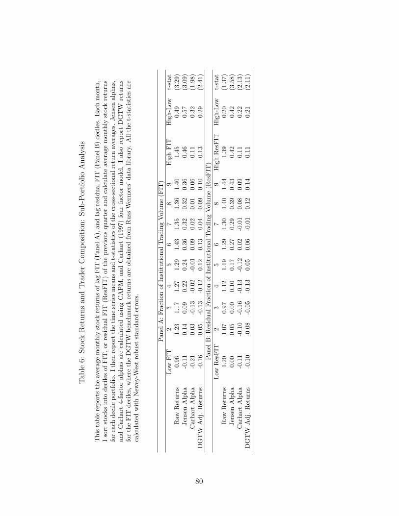
Tab

le6:

Sto

ckR

eturn

san

dTra

der

Com

pos

itio

n:

Sub-P

ortf

olio

Anal

ysi

s

Thi

sta

ble

repo

rts

the

aver

age

mon

thly

stoc

kre

turn

sof

lag

FIT

(Pan

elA

),an

dla

gre

sidu

alFIT

(Pan

elB

)de

cile

s.E

ach

mon

th,

Iso

rtst

ocks

into

deci

les

ofFIT

,or

resi

dual

FIT

(Res

FIT

)of

the

prev

ious

quar

ter

and

calc

ulat

eav

erag

em

onth

lyst

ock

retu

rns

forea

chde

cile

port

folio

.Ith

enre

port

the

tim

ese

ries

mea

nsan

dt-

stat

isti

csof

the

cros

s-se

ctio

nalr

etur

nav

erag

es.

Jens

enal

phas

,an

dC

arha

rt4-

fact

oral

phas

are

calc

ulat

edus

ing

CA

PM

,an

dC

arha

rt(1

997)

four

fact

orm

odel

.I

also

repo

rtD

GT

Wre

turn

sfo

rth

eFIT

deci

les,

whe

reth

eD

GT

Wbe

nchm

ark

retu

rns

are

obta

ined

from

Rus

sW

erm

ers’

data

libra

ry.

All

the

t-st

atis

tics

are

calc

ulat

edw

ith

New

ey-W

est

robu

stst

anda

rder

rors

.

Pan

elA

:Fr

acti

onof

Inst

itut

iona

lTra

ding

Vol

ume

(FIT

)Low

FIT

23

45

67

89

Hig

hFIT

Hig

h-Low

t-st

atR

awR

etur

ns0.

961.

231.

171.

271.

291.

431.

351.

361.

401.

450.

49(3

.29)

Jens

enA

lpha

-0.1

10.

140.

090.

220.

240.

360.

320.

320.

360.

460.

57(3

.09)

Car

hart

Alp

ha-0

.21

0.03

-0.1

3-0

.02

-0.0

10.

090.

020.

010.

060.

110.

32(1

.98)

DG

TW

Adj

.R

etur

ns-0

.16

0.05

-0.1

3-0

.12

0.12

0.13

0.04

0.09

0.10

0.13

0.29

(2.4

1)Pan

elB

:R

esid

ualFr

acti

onof

Inst

itut

iona

lTra

ding

Vol

ume

(Res

FIT

)Low

Res

FIT

23

45

67

89

Hig

hR

esFIT

Hig

h-Low

t-st

atR

awR

etur

ns1.

201.

070.

971.

121.

191.

291.

301.

401.

441.

390.

20(1

.37)

Jens

enA

lpha

0.00

0.05

0.00

0.10

0.17

0.27

0.29

0.39

0.43

0.42

0.42

(3.5

8)C

arha

rtA

lpha

-0.1

1-0

.10

-0.1

6-0

.13

-0.1

20.

02-0

.01

0.08

0.09

0.11

0.22

(2.1

3)D

GT

WA

dj.

Ret

urns

-0.1

0-0

.08

-0.0

5-0

.13

0.05

0.06

-0.0

10.

120.

140.

110.

21(2

.11)

80

Table 7: Stock Returns of Portfolios Double Sorted on FIT and Illiquidity

This table reports the average monthly stock returns of portfolios two-dimensionally sorted on lagFIT and stock illiquidity. Each month, I sort stocks into deciles of lag of the previous quarter andcalculate average monthly stock returns for each two-dimensional portfolios. The stock illiquiditymeasure is calculated following Amihud (2002). I then report the time series means and t-statisticsof the cross-sectional return averages. All the t-statistics are calculated with Newey-West robuststandard errors.

Low FIT 2 3 4 High FIT High-Low t-statLiquid 0.67 0.93 1.19 1.24 1.36 0.69 (2.63)

2 0.65 1.04 1.25 1.36 1.47 0.82 (4.85)3 0.72 0.96 1.30 1.39 1.36 0.64 (3.91)4 0.97 1.28 1.58 1.39 1.47 0.49 (3.11)

Illiquid 1.17 1.67 1.59 1.60 1.44 0.28 (2.06)Liquid-Illiquid 0.41 (1.74)

81

Tab

le8:

Mom

entu

man

dTra

der

Com

pos

itio

n:

Sub-P

ortf

olio

Anal

ysi

s

Iap

ply

6-m

onth

form

atio

n/6-

mon

thho

ldin

gm

omen

tum

stra

tegy

and

exam

ine

mom

entu

mpr

ofits

acro

sste

rcile

sof

FIT

(Pan

elA

),an

dR

esid

ual

FIT

(Pan

elB

).In

part

icul

ar,

atth

ebe

ginn

ing

ofea

chm

onth

,an

inde

pend

ent

sort

isus

edto

rank

stoc

ksin

tode

cile

sof

thei

rpa

stsi

x-m

onth

retu

rns

and

thre

egr

oups

ofon

equ

arte

rla

gFIT

(Pan

elA

),or

resi

dual

FIT

(Pan

elB

).T

hera

nked

stoc

ksar

eas

sign

edto

one

of30

two

dim

ensi

onal

lyso

rted

port

folio

sw

hich

are

held

for

six

mon

ths.

Inor

der

toav

oid

the

mic

rost

ruct

ure

effec

t,th

ere

isan

one-

mon

thin

terv

albe

twee

nth

epo

rtfo

liofo

rmat

ion

date

and

the

six-

mon

thre

turn

mea

sure

men

tpe

riod

asin

Jega

dees

han

dT

itm

an(1

993)

.T

het-

stat

isti

csar

eca

lcul

ated

wit

hN

ewey

-Wes

tro

bust

stan

dard

erro

rs.

Los

er2

34

56

78

9W

inne

rW

inne

r-

Los

ert-

stat

Pan

elA

:Fr

acti

onof

Inst

itut

iona

lTra

ding

Vol

ume

(FIT

)Low

FIT

0.23

0.72

0.94

1.00

1.07

1.13

1.15

1.19

1.40

1.70

1.48

(6.2

4)M

ed.

FIT

0.64

1.05

1.13

1.26

1.27

1.32

1.30

1.35

1.42

1.69

1.05

(4.7

2)H

igh

FIT

0.81

1.14

1.23

1.32

1.35

1.31

1.36

1.38

1.46

1.76

0.95

(4.4

6)Low

-H

igh

0.53

(3.4

0)Pan

elB

:R

esid

ualFr

acti

onof

Inst

itut

iona

lTra

ding

Vol

ume

(Res

FIT

)Low

Res

FIT

0.35

0.81

0.96

1.07

1.09

1.16

1.16

1.18

1.39

1.72

1.37

(5.6

4)M

ed.

Res

FIT

0.49

0.98

1.07

1.18

1.18

1.20

1.25

1.30

1.40

1.66

1.17

(5.4

4)H

igh

Res

FIT

0.82

1.15

1.27

1.33

1.38

1.36

1.40

1.42

1.48

1.72

0.90

(4.3

5)Low

-H

igh

0.47

(3.4

4)

82

Table 9: Quarterly Fama-Macbeth Regressions: Momentum and TraderComposition

This table reports quarterly Fama-Macbeth regressions of stock returns (constants not reported). Theindependent variable is quarterly cumulative stock returns (%). The independent variables are measuredat the end of the previous quarter. Each quarter I run a cross sectional regression and then calculatetime series means and t-stats of the coefficients. FIT, FIB and FIS are calculated following equations(1) to (6) in the paper. Betas are obtained from CRSP; ME is a firm’s market capitalization; BM isthe book-to-market ratio. Ret(-6,-1) is the cumulative return of a firm during the past six months. IOis the institutional ownership. ResAC is the residual analyst coverage. Turnover is the total quarterlyturnover. I follow Chan, Jegadeesh and Lakonishok (1996) to transform the independent variables intostandardized ranks between 0 and 1. There is one-month interval before the return measurement period.The t-statistics are calculated based on Newey-West standard errors.

Models Model 1 Model 2 Model 3 Model 4 Model 5 Model 6 Model 7Ret(-6,-1) 4.61 3.77 4.84 6.25 4.99 5.09 6.18t-stat (5.80) (5.00) (5.62) (6.23) (5.71) (5.64) (6.05)Beta -0.57 -0.82 -0.65 -0.48 -0.60 -0.67 -0.51t-stat (-0.63) (-0.93) (-0.76) (-0.62) (-0.66) (-0.78) (-0.65)Ln(ME)(t-1) -0.85 -0.90 -0.97 1.41 -0.95 -1.04 1.27t-stat (-1.12) (-1.09) (-1.18) (1.60) (-1.24) (-1.27) (1.46)BE/ME 1.46 1.46 1.43 1.95 1.44 1.42 1.96t-stat (3.10) (3.09) (3.08) (3.67) (3.07) (3.07) (3.69)Turnover(t-1) -1.64 -1.75t-stat (-2.43) (-2.63)Res-AnalystCoverage(t-1) 0.92 0.87t-stat (1.67) (1.59)FIT(t-1) 3.52 3.09 2.39t-stat (5.02) (5.25) (4.20)FIB(t-1) 1.82 1.61 1.00t-stat (2.96) (2.81) (1.82)FIS(t-1) 2.36 2.20 1.80t-stat (3.99) (3.88) (3.24)IO(t-1) 2.54 0.91 0.66 0.64 0.58t-stat (3.03) (1.16) (0.92) (0.83) (0.84)FIT(t-1)*Ret(-6,-1) -4.21 -3.88 -2.78t-stat (-4.08) (-3.91) (-3.02)FIB(t-1)*Ret(-6,-1) -1.98 -1.88 -0.94t-stat (-2.07) (-1.96) (-1.01)FIS(t-1)*Ret(-6,-1) -2.87 -2.81 -2.05t-stat (-2.98) (-2.86) (-2.26)IO(t-1)*Ret(-6,-1) -2.57 -0.69 0.10 -0.29 0.09t-stat (-2.45) (-0.66) (0.09) (-0.27) (0.08)Ln(ME)(t-1)*Ret(-6,-1) -4.82 -4.70t-stat (-4.91) (-4.86)BM*Ret(-6,-1) -1.06 -1.10t-stat (-1.68) (-1.65)Turnover(t-1)*Ret(-6,-1) 2.17 2.40t-stat (2.23) (2.48)ResAC(t-1)*Ret(-6,-1) -1.07 -0.98t-stat (-1.25) (-1.16)

Average Adj. R-square 0.0520 0.0534 0.0603 0.0641 0.0543 0.0567 0.065083

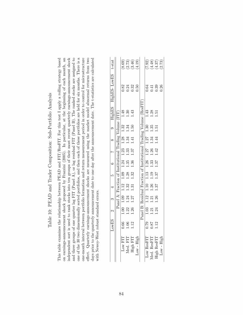
Tab

le10

:P

EA

Dan

dTra

der

Com

pos

itio

n:

Sub-P

ortf

olio

Anal

ysi

s

Thi

sta

ble

exam

ines

the

rela

tion

ship

betw

een

PE

AD

and

FIT

/Res

FIT

.Fo

rth

iste

stI

appl

ya

rolli

ngst

rate

gyba

sed

onea

rnin

gs-a

nnou

ncem

ent

shoc

kpr

opos

edby

Fraz

zini

(200

5).

Inpa

rtic

ular

,at

the

begi

nnin

gof

each

mon

th,

anin

depe

nden

tso

rtis

used

tora

nkst

ocks

into

ten

grou

psof

thei

rm

ost

rece

ntqu

arte

rly

earn

ings

-ann

ounc

emen

tsh

ock

and

thre

egr

oups

ofon

equ

arte

rla

gFIT

(Pan

elA

),or

lag

resi

dual

FIT

(Pan

elB

).T

hera

nked

stoc

ksar

eas

sign

edto

one

ofth

e30

two

dim

ensi

onal

lyso

rted

port

folio

s,an

dth

enea

chof

thes

epo

rtfo

lios

are

held

for

six

mon

ths.

The

reis

aon

e-m

onth

inte

rval

betw

een

port

folio

form

atio

nan

dre

turn

mea

sure

men

tpe

riod

inor

der

toco

ntro

lfor

mic

rost

ruct

ure

effec

t.Q

uart

erly

earn

ings

-ann

ounc

emen

tsh

ocks

are

mea

sure

dus

ing

the

mar

ket

mod

elab

norm

alre

turn

sfr

omtw

oda

yspr

ior

toth

equ

arte

rly

anno

unce

men

tda

teto

one

day

afte

rth

ean

noun

cem

ent

date

.T

het-

stat

isti

csar

eca

lcul

ated

wit

hN

ewey

-Wes

tro

bust

stan

dard

erro

rs.

Low

ES

23

45

67

89

Hig

hES

Hig

hES-

Low

ES

t-st

atPan

elA

:Fr

acti

onof

Inst

itut

iona

lTra

ding

Vol

ume

(FIT

)Low

FIT

0.66

1.00

1.09

1.12

1.09

1.24

1.23

1.28

1.32

1.48

0.82

(8.6

9)M

ed.

FIT

1.06

1.22

1.24

1.32

1.28

1.35

1.33

1.34

1.34

1.30

0.24

(2.7

3)H

igh

FIT

1.12

1.26

1.27

1.31

1.32

1.36

1.37

1.41

1.50

1.43

0.32

(3.4

6)Low

-H

igh

0.50

(4.1

9)Pan

elB

:R

esid

ualFr

acti

onof

Inst

itut

iona

lTra

ding

Vol

ume

(Res

FIT

)Low

Res

FIT

0.79

1.03

1.12

1.10

1.13

1.26

1.27

1.27

1.30

1.43

0.64

(7.9

2)M

ed.

Res

FIT

0.87

1.21

1.21

1.26

1.19

1.33

1.26

1.34

1.35

1.28

0.41

(4.4

8)H

igh

Res

FIT

1.12

1.24

1.26

1.37

1.37

1.37

1.42

1.44

1.51

1.51

0.39

(4.3

7)Low

-H

igh

0.26

(2.7

3)

84

Table 11: Quarterly Fama-Macbeth Regressions: PEAD and Trader Com-position

This table reports quarterly Fama-Macbeth regressions of stock returns (constants not reported). Theindependent variable is quarterly cumulative stock returns (%). The independent variables are measuredat the end of the previous quarter. Each quarter I run a cross sectional regression and then calculate timeseries means and t-stats of the coefficients. EarningsShock is the earnings-announcement shock measuredusing the market model abnormal returns from two days prior to the quarterly announcement date to oneday after the announcement date. FIT, FIB, and FIS are calculated following equations (1) to (6) in thepaper. Betas are obtained from CRSP; ME is a firm’s market capitalization; BM is the book-to-marketratio. Ret(-6,-1) is the cumulative return of a firm during the past six months. IO is the institutionalownership. I follow Chan, Jegadeesh and Lakonishok (1996) to transform the independent variables intostandardized ranks between 0 and 1. To facilitate the evaluation of economic significance, I follow Chan,Jegadeesh, and Lakonishok (1996) to transform the independent variables into standardized ranks between0 and 1. To control for the microstructure effect, there is one-month interval before the return measurementperiod. The t-statistics are calculated based on Newey-West standard errors.

Models Model 1 Model 2 Model 3 Model 4 Model 5 Model 6 Model 7EarningsShock 1.95 1.90 2.42 3.15 2.23 2.55 3.26t-stat (4.28) (4.30) (4.68) (5.47) (4.28) (4.78) (5.49)Beta -0.64 -0.85 -0.71 -0.70 -0.66 -0.72 -0.70t-stat (-0.74) (-1.00) (-0.87) (-0.85) (-0.75) (-0.86) (-0.84)Ln(ME)(t-1) -0.97 -1.01 -1.10 0.42 -1.09 -1.19 0.34t-stat (-1.24) (-1.18) (-1.30) (0.46) (-1.37) (-1.38) (0.37)BE/ME 1.34 1.36 1.33 1.33 1.32 1.31 1.31t-stat (2.75) (2.77) (2.75) (2.76) (2.72) (2.76) (2.76)Ret(-6,-1) 2.20 2.16 2.21 2.20 2.22 2.24 2.23t-stat (3.52) (3.45) (3.56) (3.53) (3.53) (3.49) (3.46)FIT(t-1) 2.54 1.94 1.80t-stat (4.33) (3.74) (3.42)FIB(t-1) 1.59 1.19 0.97t-stat (2.65) (2.13) (1.73)FIS(t-1) 1.51 1.26 1.28t-stat (3.37) (2.65) (2.72)IO(t-1) 2.22 1.29 0.71 1.11 0.57t-stat (3.32) (2.05) (1.19) (1.80) (0.98)FIT(t-1)*EarningsShock -2.63 -1.80 -1.54t-stat (-3.80) (-2.43) (-1.99)FIB(t-1)*EarningsShock -1.42 -0.79 -0.41t-stat (-1.54) (-0.88) (-0.46)FIS(t-1)*EarningsShock -1.73 -1.44 -1.45t-stat (-2.34) (-1.89) (-1.95)IO(t-1)*EarningsShock -2.40 -1.66 -0.50 -1.47 -0.37t-stat (-3.44) (-2.17) (-0.70) (-1.92) (-0.52)Ln(ME)(t-1)*EarningsShock -3.07 -3.07t-stat (-4.17) (-4.13)

Average Adj. R-square 0.0535 0.0545 0.0562 0.0568 0.0548 0.0571 0.0576

85

Tab

le12

:V

alue

Pre

miu

man

dTra

der

Com

pos

itio

n:

Sub-P

ortf

olio

Anal

ysi

s

Thi

sta

ble

exam

ines

the

rela

tion

ship

betw

een

the

valu

epr

emiu

man

dtr

ader

com

posi

tion

.In

part

icul

ar,at

the

begi

nnin

gof

each

mon

th,a

nin

depe

nden

tso

rtis

used

tora

nkst

ocks

onte

ngr

oups

ofth

eir

book

-to-

mar

ket

rati

osan

dth

ree

grou

psof

one

quar

ter

lag

FIT

(Pan

elA

),or

lag

resi

dual

FIT

(Pan

elB

).T

hera

nked

stoc

ksar

eas

sign

edto

one

ofth

e30

two-

dim

ensi

onal

lyso

rted

port

folio

s,an

dI

then

exam

ine

the

tim

e-se

ries

mea

nsan

dt-

stat

isti

csof

the

mon

thly

retu

rns

ofth

ese

port

folio

s.T

het-

stat

isti

csar

eca

lcul

ated

wit

hN

ewey

-Wes

tro

bust

stan

dard

erro

rs.

Low

BM

23

45

67

89

Hig

hB

MH

ighB

M-

Low

BM

t-st

atPan

elA

:Fr

acti

onof

Inst

itut

iona

lTra

ding

Vol

ume

(FIT

)Low

FIT

0.58

0.89

1.08

1.17

1.38

1.08

1.26

1.30

1.32

1.48

0.90

(3.3

7)M

ed.

FIT

1.04

1.15

1.26

1.28

1.41

1.26

1.43

1.38

1.47

1.72

0.68

(2.9

5)H

igh

FIT

1.28

1.31

1.34

1.40

1.35

1.40

1.39

1.46

1.48

1.55

0.27

(1.4

1)Low

-H

igh

0.63

(2.8

5)Pan

elB

:R

esid

ualFr

acti

onof

Inst

itut

iona

lTra

ding

Vol

ume

(Res

FIT

)Low

Res

FIT

0.72

0.94

1.14

1.10

1.36

1.16

1.23

1.32

1.34

1.45

0.73

(3.0

7)M

ed.

Res

FIT

0.78

1.03

1.26

1.39

1.35

1.35

1.33

1.33

1.36

1.65

0.87

(3.5

3)H

igh

Res

FIT

1.30

1.40

1.33

1.37

1.43

1.27

1.47

1.48

1.58

1.62

0.32

(1.5

1)Low

-H

igh

0.41

(2.1

9)

86

Table 13: Monthly Fama-Macbeth Regressions: Value premium and TraderComposition

This table reports monthly Fama-Macbeth regressions of stock returns (constants not reported). Theindependent variable is monthly stock returns (%). The independent variables are measured at theend of the previous month. Each month I run a cross sectional regression and then calculate timeseries means and t-stats of the coefficients. FIT, FIB, and FIS are calculated following equations (1)to (6) in the paper. Betas are obtained from CRSP; ME is a firm’s market capitalization; BM is thebook-to-market ratio. Ret(-6,-1) is the cumulative return of a firm during the past six months skippinga month. IO is the institutional ownership at the beginning of the quarter. To facilitate the evaluationeconomic significance, I follow Chan, Jegadeesh, and Lakonishok (1996) to transform the independentvariables into standardized ranks between 0 and 1. The t-statistics are calculated based on Newey-Weststandard errors.

Models Model 1 Model 2 Model 3 Model 4 Model 5 Model 6 Model 7BE/ME 0.84 0.83 0.93 0.89 0.83 0.89 0.86t-stat (3.63) (3.74) (3.82) (3.45) (3.68) (3.82) (3.50)Beta -0.10 -0.19 -0.13 -0.13 -0.12 -0.14 -0.14t-stat (-0.35) (-0.63) (-0.44) (-0.42) (-0.41) (-0.49) (-0.48)Ln(ME)(t-1) -0.37 -0.38 -0.42 -0.46 -0.39 -0.43 -0.45t-stat (-1.45) (-1.39) (-1.53) (-1.40) (-1.52) (-1.60) (-1.41)Ret(-6,-1) 0.68 0.67 0.68 0.68 0.73 0.74 0.74t-stat (3.11) (3.06) (3.16) (3.16) (3.24) (3.32) (3.32)FIT(t-1) 0.92 0.71 0.70t-stat (3.92) (2.99) (2.94)FIB(t-1) 0.31 0.20 0.18t-stat (1.70) (1.09) (0.98)FIS(t-1) 0.70 0.60 0.61t-stat (3.80) (3.24) (3.31)IO(t-1) 0.79 0.38 0.40 0.33 0.33t-stat (3.52) (1.70) (1.65) (1.58) (1.46)FIT(t-1)*BM -0.79 -0.56 -0.54t-stat (-3.02) (-1.89) (-1.84)FIB(t-1)*BM -0.29 -0.17 -0.14t-stat (-1.20) (-0.69) (-0.57)FIS(t-1)*BM -0.56 -0.45 -0.45t-stat (-2.21) (-1.69) (-1.71)IO(t-1)*BM -0.73 -0.40 -0.43 -0.36 -0.36t-stat (-2.67) (-1.29) (-1.29) (-1.21) (-1.15)Ln(ME)(t-1)*BM 0.09 0.04t-stat (0.31) (0.15)

Average Adj. R-square 0.0479 0.0480 0.0512 0.0520 0.0495 0.0526 0.0533

87

Tab

le14

:M

omen

tum

and

Tra

der

Com

pos

itio

n:

Sub-P

erio

dA

nal

ysi

s

Iap

ply

6-m

onth

form

atio

n/6-

mon

thho

ldin

gm

omen

tum

stra

tegy

and

exam

ine

mom

entu

mpr

ofits

acro

sste

rcile

sof

FIT

duri

ngth

eth

ree

sub-

peri

ods

of19

80-1

987

(Pan

elA

),19

88-1

996

(Pan

elB

)an

d19

97-2

005

(Pan

elC

).In

part

icul

ar,at

the

begi

nnin

gof

each

mon

th,a

nin

depe

nden

tso

rtis

used

tora

nkst

ocks

into

deci

lesof

thei

rpa

stsi

x-m

onth

retu

rnsan

dth

ree

grou

psof

one

quar

ter

lag

FIT

.T

hera

nked

stoc

ksar

eas

sign

edto

one

of30

two

dim

ensi

onal

lyso

rted

port

folio

sw

hich

are

held

for

six

mon

ths.

Inor

der

toav

oid

the

mic

rost

ruct

ure

effec

t,th

ere

isan

one-

mon

thin

terv

albe

twee

nth

epo

rtfo

liofo

rmat

ion

date

and

the

six-

mon

thre

turn

mea

sure

men

tpe

riod

asin

Jega

dees

han

dT

itm

an(1

993)

.T

het-

stat

isti

csar

eca

lcul

ated

wit

hN

ewey

-Wes

tro

bust

stan

dard

erro

rs.

Los

er2

34

56

78

9W

inne

rW

inne

r-

Los

ert-

stat

Pan

elA

:Su

b-Sa

mpl

eA

naly

sis:

1980

-198

7Low

FIT

0.09

0.95

1.31

1.28

1.35

1.47

1.29

1.36

1.51

1.48

1.38

(4.2

1)M

ed.

FIT

0.60

1.21

1.33

1.46

1.50

1.53

1.51

1.53

1.39

1.49

0.89

(2.4

9)H

igh

FIT

0.80

1.24

1.37

1.53

1.59

1.62

1.56

1.53

1.53

1.67

0.87

(2.0

9)Low

-H

igh

0.51

(1.8

0)Pan

elB

:Su

b-Sa

mpl

eA

naly

sis:

1988

-199

6Low

FIT

0.31

0.80

0.93

1.00

0.99

1.05

1.25

1.21

1.41

1.83

1.51

(4.6

5)M

ed.

FIT

0.75

1.10

1.23

1.37

1.38

1.42

1.37

1.43

1.54

1.88

1.12

(3.3

7)H

igh

FIT

0.83

1.14

1.24

1.34

1.32

1.26

1.33

1.35

1.44

1.81

0.98

(3.2

1)Low

-H

igh

0.53

(2.5

9)Pan

elC

:Su

b-Sa

mpl

eA

naly

sis:

1997

-200

5Low

FIT

0.24

0.46

0.64

0.79

0.94

0.95

0.95

1.02

1.31

1.76

1.51

(2.9

6)M

ed.

FIT

0.56

0.88

0.87

0.99

0.96

1.05

1.06

1.14

1.31

1.66

1.10

(2.5

0)H

igh

FIT

0.80

1.07

1.10

1.15

1.19

1.11

1.25

1.30

1.44

1.77

0.97

(2.5

2)Low

-H

igh

0.54

(2.7

3)

88

Tab

le15

:P

EA

Dan

dTra

der

Com

pos

itio

n:

Sub-P

erio

dA

nal

ysi

s

Thi

sta

ble

exam

ines

the

rela

tion

ship

betw

een

PE

AD

and

FIT

duri

ngth

eth

ree

sub-

peri

ods

of19

80-1

987

(Pan

elA

),19

88-1

996

(Pan

elB

)an

d19

97-2

005

(Pan

elC

)..

Forth

iste

stIap

ply

aro

lling

stra

tegy

base

don

earn

ings

-ann

ounc

emen

tsh

ock

prop

osed

byFr

azzi

ni(2

005)

.In

part

icul

ar,a

tth

ebe

ginn

ing

ofea

chm

onth

,an

inde

pend

ent

sort

isus

edto

rank

stoc

ksin

tote

ngr

oups

ofth

eir

mos

tre

cent

quar

terl

yea

rnin

gs-a

nnou

ncem

ent

shoc

kan

dth

ree

grou

psof

one

quar

ter

lag

FIT

.T

hera

nked

stoc

ksar

eas

sign

edto

one

ofth

e30

two

dim

ensi

onal

lyso

rted

port

folio

s,an

dth

enea

chof

thes

epo

rtfo

lios

are

held

for

six

mon

ths.

The

reis

aon

e-m

onth

inte

rval

betw

een

port

folio

form

atio

nan

dre

turn

mea

sure

men

tpe

riod

inor

der

toco

ntro

lfo

rm

icro

stru

ctur

eeff

ect.

Qua

rter

lyea

rnin

gs-a

nnou

ncem

ent

shoc

ksar

em

easu

red

usin

gth

em

arke

tm

odel

abno

rmal

retu

rns

from

two

days

prio

rto

the

quar

terl

yan

noun

cem

ent

date

toon

eda

yaf

ter

the

anno

unce

men

tda

te.

The

t-st

atis

tics

are

calc

ulat

edw

ith

New

ey-W

est

robu

stst

anda

rder

rors

.

Low

ES

23

45

67

89

Hig

hES

Hig

hES-

Low

ES

t-st

atPan

elA

:Su

b-Sa

mpl

eA

naly

sis:

1980

-198

7Low

FIT

0.30

0.99

1.17

1.35

1.23

1.50

1.37

1.41

1.39

1.31

1.00

(6.6

6)M

ed.

FIT

0.79

1.20

1.25

1.58

1.44

1.63

1.47

1.45

1.50

1.39

0.60

(4.6

7)H

igh

FIT

1.15

1.27

1.35

1.51

1.51

1.54

1.58

1.57

1.72

1.62

0.47

(3.0

1)Low

-H

igh

0.54

(3.1

1)Pan

elB

:Su

b-Sa

mpl

eA

naly

sis:

1988

-199

6Low

FIT

0.99

1.26

1.16

1.06

1.12

1.15

1.25

1.29

1.36

1.73

0.74

(4.7

0)M

ed.

FIT

1.34

1.33

1.35

1.41

1.33

1.39

1.31

1.34

1.42

1.45

0.11

(0.8

1)H

igh

FIT

1.11

1.38

1.26

1.24

1.27

1.35

1.32

1.40

1.42

1.42

0.31

(1.9

7)Low

-H

igh

0.43

(2.0

4)Pan

elC

:Su

b-Sa

mpl

eA

naly

sis:

1997

-200

5Low

FIT

0.60

0.73

0.96

0.98

0.95

1.13

1.11

1.16

1.22

1.35

0.75

(4.1

4)M

ed.

FIT

0.99

1.13

1.11

1.01

1.08

1.08

1.23

1.24

1.11

1.05

0.07

(0.4

0)H

igh

FIT

1.09

1.10

1.22

1.22

1.21

1.23

1.26

1.28

1.40

1.29

0.20

(1.2

0)Low

-H

igh

0.55

(2.4

6)

89

Tab

le16

:V

alue

Pre

miu

man

dTra

der

Com

pos

itio

n:

Sub-P

erio

dA

nal

ysi

s

Thi

sta

ble

exam

ines

the

rela

tion

ship

betw

een

the

valu

epr

emiu

man

dFIT

duri

ngth

eth

ree

sub-

peri

ods

of19

80-1

987

(Pan

elA

),19

88-1

996

(Pan

elB

)an

d19

97-2

005

(Pan

elC

)..

Inpa

rtic

ular

,at

the

begi

nnin

gof

each

mon

th,

anin

depe

nden

tso

rtis

used

tora

nkst

ocks

onte

ngr

oups

ofth

eir

book

-to-

mar

ket

rati

osan

dth

ree

grou

psof

one

quar

ter

lag

FIT

.The

rank

edst

ocks

are

assi

gned

toon

eof

the

30tw

o-di

men

sion

ally

sort

edpo

rtfo

lios,

and

Ith

enex

amin

eth

eti

me-

seri

esm

eans

and

t-st

atis

tics

ofth

em

onth

lyre

turn

sof

thes

epo

rtfo

lios.

The

t-st

atis

tics

are

calc

ulat

edw

ith

New

ey-W

est

robu

stst

anda

rder

rors

.

Low

BM

23

45

67

89

Hig

hB

MH

ighB

M-

Low

BM

t-st

atPan

elA

:Su

b-Sa

mpl

eA

naly

sis:

1980

-198

7Low

FIT

0.13

0.73

0.85

1.33

1.67

1.39

1.65

1.41

1.48

1.70

1.58

(2.8

2)M

ed.

FIT

0.99

1.27

1.31

1.61

1.77

1.33

1.87

1.44

1.88

2.10

1.11

(2.8

3)H

igh

FIT

1.37

1.36

1.54

1.66

1.54

1.66

1.82

1.57

1.60

1.74

0.38

(1.1

1)Low

-H

igh

1.20

(3.2

0)Pan

elB

:Su

b-Sa

mpl

eA

naly

sis:

1988

-199

6Low

FIT

0.96

1.21

1.39

1.22

1.38

0.96

1.09

1.41

1.04

1.32

0.36

(1.2

2)M

ed.

FIT

1.31

1.14

1.25

1.28

1.34

1.37

1.36

1.39

1.39

1.57

0.26

(0.6

5)H

igh

FIT

1.20

1.24

1.41

1.38

1.45

1.28

1.34

1.60

1.44

1.48

0.28

(1.0

4)Low

-H

igh

0.08

(0.2

7)Pan

elC

:Su

b-Sa

mpl

eA

naly

sis:

1997

-200

5Low

FIT

0.58

0.68

0.95

0.97

1.13

0.94

1.10

1.09

1.46

1.45

0.88

(1.8

1)M

ed.

FIT

0.81

1.05

1.23

1.02

1.19

1.09

1.15

1.33

1.21

1.55

0.75

(1.9

9)H

igh

FIT

1.28

1.34

1.09

1.21

1.08

1.30

1.10

1.22

1.43

1.45

0.17

(0.4

5)Low

-H

igh

0.70

(1.6

9)

90

Table 17: Calculation of PPIndex

In each cross-section, I put stocks into ten portfolios according to their cumulativereturns during the past six months. The portfolios are sorted in ascending orderfrom extreme past losers to extreme past winners. Then I assign discrete PPIndexfrom -5 to 5 to the past-return portfolios, where -5 is assigned to the bottom past-return decile and 5 assigned to the top past-return decile.

Return Portfolios Loser 2 3 4 5 6 7 8 9 WinnerPpindex -5 -4 -3 -2 -1 1 2 3 4 5

Table 18: Summary Statistics of the MT Measure

I calculate the MT measure for each firm-quarter during the 1982-2005 on a two-year rollingbasis following equation (1). In particular, for each individual stock I calculate the MTmeasures during two-year estimation periods and apply them to the subsequent quarters.This table reports for the first quarter of every three-year period the number of firms as wellas mean, standard deviation, t-statistic, median, 10% cutoff, 1/4 quartile, 3/4 quartile and90% cutoff of the MT measures. I also report these statistics for the whole sample period.There are in total 367,337 firm-quarter observations with available MT measure.

Quarter Obs Mean Std. t-stat 10P 25P Median 75P 90PTotal 367,337 0.31 2.31 81.88 -2.62 -1.27 0.25 1.87 3.52

1st Quarter, 1982 2,552 0.39 2.24 8.91 -2.35 -1.14 0.35 1.98 3.451st Quarter, 1985 2,786 0.38 2.20 9.13 -2.37 -1.09 0.37 1.82 3.241st Quarter, 1988 3,088 0.23 2.25 5.63 -2.57 -1.27 0.17 1.62 3.331st Quarter, 1991 3,145 0.33 2.30 8.16 -2.64 -1.22 0.36 1.88 3.431st Quarter, 1994 3,720 0.38 2.33 9.99 -2.62 -1.23 0.27 1.98 3.811st Quarter, 1997 4,731 0.37 2.37 10.72 -2.54 -1.29 0.14 2.00 4.001st Quarter, 2000 4,999 0.31 2.24 9.64 -2.53 -1.19 0.25 1.76 3.351st Quarter, 2003 4,499 0.15 2.42 4.06 -3.14 -1.56 0.19 1.82 3.36

91

Table 19: The MT Measure and Firm Characteristics

This table describes the relationships between the MT measures and firmcharacteristics. In particular, for each month of the sample period, I sortstocks into quintiles according to the MT measures of month t and calculateaverage return, size, book-to-market ratio, demeaned turnover, coverage,and MT measures of each quintile. The time series means and t-statisticsof the firm characteristics are reported. Return is stock return of montht. Size is the natural log of market capitalization at the end of month t-1.BE/ME is the book-to-market ratio of month t. Turnover is demeanedturnover of month t-1. Coverage is the residual analyst coverage of montht-1 calculated following Griffin and Lemmon (2002). RetVolty is returnvolatility, measured as standard deviation of daily stock returns in the 25trading days up to the end of month t-1. FirmAge is age of a firm measuredas the number of months from the firm’s first CRSP monthly return record.

MT Level Low 2 3 4 High High-Low t-statReturn 1.01 1.21 1.25 1.17 1.17 0.16 0.87

Size 19.96 20.24 20.30 20.20 19.78 -0.18 -15.25BM 0.69 0.68 0.66 0.63 0.57 -0.12 -18.49

Turnover 0.01 0.00 0.00 0.01 0.05 0.04 17.70Coverage 0.64 0.36 0.32 0.14 -0.15 -0.79 -17.56RetVolty 0.024 0.020 0.021 0.022 0.028 0.004 13.21FirmAge 196 232 231 206 143 -53 -40.43

MT -2.47 -0.84 0.23 1.35 3.28 5.74

92

Tab

le20

:R

eturn

Mom

entu

mA

cros

sM

TG

roups:

1982

-200

5

Iso

rtst

ocks

inde

pend

entl

yin

toth

ree

grou

psof

MT

and

ten

grou

psof

past

perf

orm

ance

,an

dca

lcul

ate

profi

tsof

six-

mon

thfo

rmat

ion/

six-

mon

thho

ldin

gst

rate

gyfo

llow

ing

Jega

dees

han

dT

itm

an(2

001)

for

each

MT

grou

p.Sp

ecifi

cally

,at

the

begi

nnin

gof

mon

tht,

Iso

rtst

ocks

into

thre

egr

oups

ofth

eM

Tm

easu

res

and

deci

les

ofcu

mul

ativ

est

ock

retu

rns

duri

ngth

esi

x-m

onth

peri

odup

toth

een

dof

mon

tht-

1.I

then

hold

thes

epo

rtfo

lios

for

six

mon

ths

from

the

begi

nnin

gof

mon

tht

and

repo

rtav

erag

epo

rtfo

liore

turn

sin

Pan

elA

.Pan

elB

repo

rts

the

resu

lts

ofFa

ma-

Fren

chth

ree-

fact

orm

odel

ofth

em

omen

tum

profi

tsof

the

low

,med

ium

and

high

MT

terc

iles.

The

t-st

atis

tics

are

calc

ulat

edw

ith

New

ey-W

est

robu

stst

anda

rder

rors

.

Pan

elA

:M

omen

tum

Pro

fits

Acr

oss

MT

Ter

cile

sM

TLev

elLos

er2

34

56

78

9W

inne

rW

inne

r-

Los

ert-

stat

Low

0.61

0.99

1.20

1.21

1.22

1.20

1.25

1.28

1.37

1.69

1.08

(2.9

5)M

ediu

m0.

621.

051.

231.

271.

331.

351.

361.

431.

541.

831.

21(3

.48)

Hig

h0.

220.

941.

001.

191.

191.

251.

301.

331.

481.

831.

61(4

.72)

Hig

h-

Low

0.53

(3.2

1)Pan

elB

:Fa

ma-

Fren

ch3

Fact

orR

egre

ssio

nsof

Mom

entu

mP

rofit

sM

TLev

elIn

terc

ept

MK

TSM

BH

ML

Low

1.32

-0.3

30.

31-0

.08

(3.5

2)(-

3.05

)(1

.34)

(-0.

30)

Med

ium

1.43

-0.2

90.

28-0

.08

(3.8

2)(-

2.62

)(1

.21)

(-0.

34)

Hig

h1.

80-0

.20

0.26

-0.1

7(4

.84)

(-2.

02)

(1.2

4)(-

0.76

)H

igh

-Low

0.48

0.13

-0.0

5-0

.09

(3.0

2)(3

.19)

(-0.

70)

(-1.

04)

93

Table 21: Six-Month/Six-Month Strategy: Two-Dimensional Sort on Sizeand MT: 1982-2005

At the beginning of month t, I sort stocks independently into three groups of the MT measure, threegroups of market capitalization at the end of month t-1, and quintiles of cumulative returns over thesix-month perioud up to the end of month t-1. Following the six-month-holding/six-month-formationstrategy of Jegadeesh and Titman (2001), I hold these three-dimensionally sorted portfolios for sixmonths. Panel A reports the average monthly returns of the portfolios and Panel B reports the compar-isons of momentum profits across the size-MT groups. Average size and average MT are measured indecile ranks. Specifically, I assign deciles ranks of size and MT to the stocks in each cross-section, where1 is assigned to the bottom deicle and 10 to the top decile. I then calculate time series averages of thecross sectional mean ranks of size and MT for each size-MT group.

Panel A: Momentum Profits Across Size-MT groupsSize MT Loser 2 3 4 Winner W-L t-stat Ave.Size Ave.MT

Small Low 0.65 1.15 1.13 1.32 1.64 0.99 (3.52) 2.17 2.07Small Med 0.85 1.24 1.33 1.49 1.78 0.93 (3.67) 2.28 5.51Small High 0.36 1.05 1.22 1.40 1.80 1.44 (5.90) 2.18 9.01Med. Low 0.82 1.20 1.26 1.20 1.51 0.69 (2.44) 5.48 2.20Med. Med 0.78 1.25 1.32 1.39 1.70 0.92 (3.39) 5.54 5.51Med. High 0.62 1.05 1.21 1.31 1.69 1.07 (3.72) 5.48 8.79Big Low 1.03 1.26 1.26 1.27 1.41 0.37 (1.25) 8.81 2.35Big Med 0.96 1.25 1.34 1.31 1.54 0.58 (1.94) 8.86 5.49Big High 0.79 1.19 1.24 1.23 1.60 0.81 (2.48) 8.70 8.54

Panel B: Comparisons of Momentum ProfitsSize Level

Small Med. Big S-B t-statLow 0.99 0.69 0.37 0.62 (3.60)

MT level Med. 0.93 0.92 0.58 0.35 (1.89)High 1.44 1.07 0.81 0.63 (2.99)H-L 0.45 0.38 0.44

t-stat (2.73) (2.38) (2.22)

94

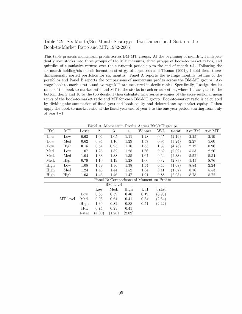
Table 22: Six-Month/Six-Month Strategy: Two-Dimensional Sort on theBook-to-Market Ratio and MT: 1982-2005

This table presents momentum profits across BM-MT groups. At the beginning of month t, I indepen-dently sort stocks into three groups of the MT measures, three groups of book-to-market ratios, andquintiles of cumulative returns over the six-month period up to the end of month t-1. Following thesix-month holding/six-month formation strategy of Jegadeesh and Titman (2001), I hold these three-dimensionally sorted portfolios for six months. Panel A reports the average monthly returns of theportfolios and Panel B reports the comparisons of momentum profits across the BM-MT groups. Av-erage book-to-market ratio and average MT are measured in decile ranks. Specifically, I assign decilesranks of the book-to-market ratio and MT to the stocks in each cross-section, where 1 is assigned to thebottom deicle and 10 to the top decile. I then calculate time series averages of the cross-sectional meanranks of the book-to-market ratio and MT for each BM-MT group. Book-to-market ratio is calculatedby dividing the summation of fiscal year-end book equity and deferred tax by market equity. I thenapply the book-to-market ratio at the fiscal year end of year t to the one year period starting from Julyof year t+1.

Panel A: Momentum Profits Across BM-MT groupsBM MT Loser 2 3 4 Winner W-L t-stat Ave.BM Ave.MTLow Low 0.63 1.04 1.05 1.11 1.28 0.65 (2.19) 2.25 2.19Low Med 0.62 0.94 1.16 1.29 1.57 0.95 (3.24) 2.27 5.60Low High 0.15 0.64 0.93 1.16 1.53 1.39 (4.73) 2.12 8.96Med. Low 1.07 1.26 1.32 1.28 1.66 0.59 (2.02) 5.53 2.26Med. Med 1.04 1.33 1.38 1.35 1.67 0.64 (2.33) 5.52 5.54Med. High 0.79 1.10 1.19 1.28 1.60 0.82 (2.83) 5.45 8.76High Low 1.08 1.39 1.36 1.38 1.54 0.46 (1.68) 8.84 2.24High Med 1.24 1.46 1.44 1.52 1.64 0.41 (1.57) 8.76 5.53High High 1.03 1.46 1.46 1.47 1.91 0.88 (2.95) 8.78 8.72

Panel B: Comparisons of Momentum ProfitsBM Level

Low Med. High L-H t-statLow 0.65 0.59 0.46 0.19 (0.93)

MT level Med. 0.95 0.64 0.41 0.54 (2.54)High 1.39 0.82 0.88 0.51 (2.22)H-L 0.74 0.23 0.41

t-stat (4.00) (1.28) (2.02)

95

Table 23: Six-Month/Six-Month Strategy: Two-Dimensional Sort onTurnover and MT: 1982-2005

This table presents momentum profits across turnover-MT groups. At the beginning of month t, Iindependently sort stocks into three groups of the MT measures, three groups of turnovers of month t-1,and quintiles of cumulative returns over the six-month period up to the end of month t-1. Following thesix-month holding/six-month formation strategy of Jegadeesh and Titman (2001), I hold these three-dimensionally sorted portfolios for six months. Panel A reports the average monthly returns of theportfolios and Panel B reports the comparisons of momentum profits across the turnover-MT groups.Average turnover and average MT are measured in decile ranks. Specifically, I assign deciles ranks ofturnover and MT to the stocks in each cross-section, where 1 is assigned to the bottom deicle and 10 tothe top decile. I then calculate time series averages of the cross-sectional mean ranks of turnover andMT for each turnover-MT group. Turnovers are demeaned by the cross sectional average turnovers ofNYSE/AMEX or NASDAQ stocks according to the market where the firms is listed.

Panel A: Momentum Profits across Turnover-MT groupsTO MT Loser 2 3 4 Winner W-L t-stat Ave.TO Ave.MTLow Low 0.85 1.20 1.22 1.31 1.45 0.60 (2.59) 2.21 2.24Low Med 1.00 1.26 1.35 1.41 1.59 0.59 (2.81) 2.23 5.47Low High 0.98 1.28 1.37 1.47 1.70 0.72 (3.36) 2.14 8.64Med. Low 0.92 1.27 1.25 1.31 1.54 0.61 (2.49) 5.49 2.24Med. Med 0.97 1.31 1.36 1.44 1.64 0.67 (2.77) 5.46 5.48Med. High 0.72 1.26 1.30 1.33 1.66 0.93 (3.58) 5.56 8.67High Low 0.64 1.04 1.11 1.21 1.55 0.91 (2.81) 8.70 2.12High Med 0.63 1.07 1.28 1.32 1.73 1.09 (3.74) 8.71 5.53High High 0.20 0.78 0.98 1.17 1.69 1.49 (5.10) 8.92 8.97

Panel B: Comparisons of Momentum ProfitsTurnover Level

Low Med. High H-L t-statLow 0.60 0.61 0.91 0.31 (1.64)

MT level Med. 0.59 0.67 1.09 0.51 (2.85)High 0.72 0.93 1.49 0.77 (3.87)H-L 0.12 0.32 0.59

t-stat (0.78) (2.28) (3.57)

96

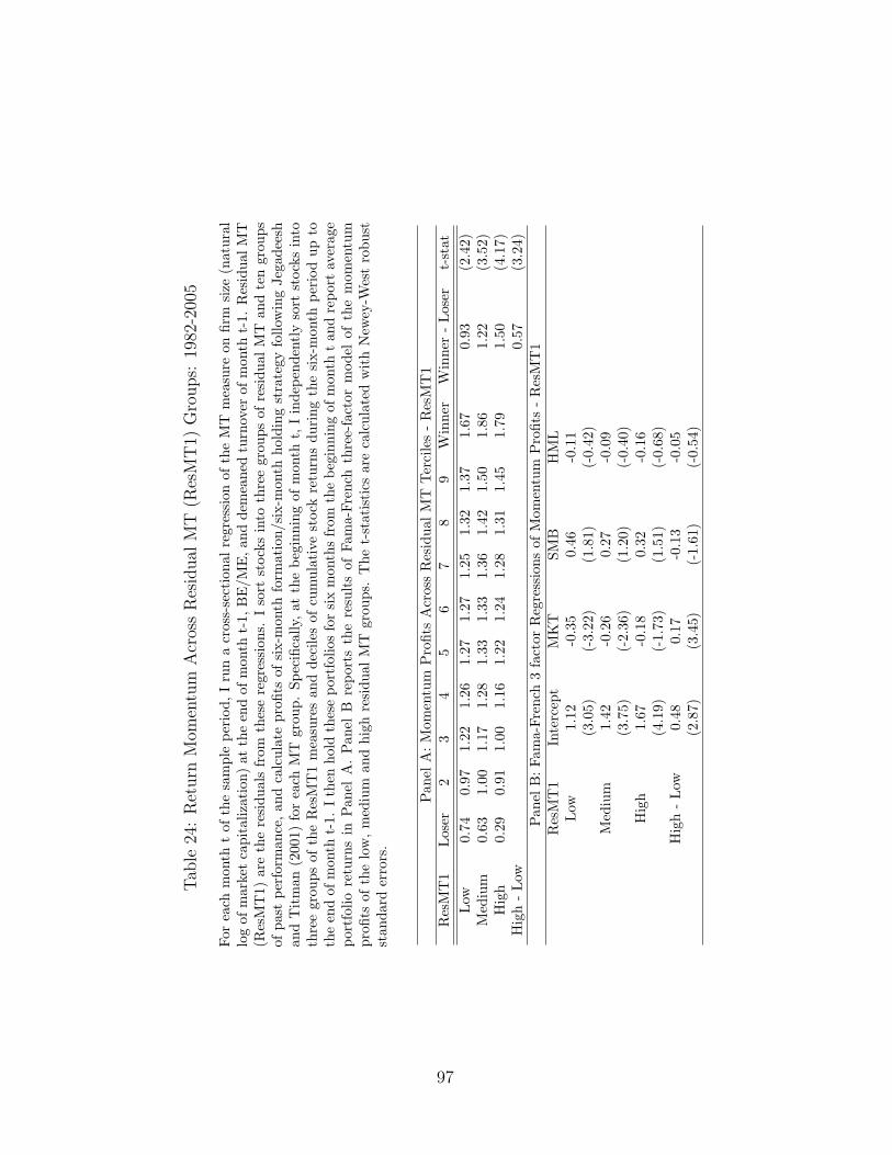
Tab

le24

:R

eturn

Mom

entu

mA

cros

sR

esid

ual

MT

(Res

MT

1)G

roups:

1982

-200

5

For

each

mon

tht

ofth

esa

mpl

epe

riod

,I

run

acr

oss-

sect

iona

lre

gres

sion

ofth

eM

Tm

easu

reon

firm

size

(nat

ural

log

ofm

arke

tca

pita

lizat

ion)

atth

een

dof

mon

tht-

1,B

E/M

E,a

ndde

mea

ned

turn

over

ofm

onth

t-1.

Res

idua

lMT

(Res

MT

1)ar

eth

ere

sidu

als

from

thes

ere

gres

sion

s.I

sort

stoc

ksin

toth

ree

grou

psof

resi

dual

MT

and

ten

grou

psof

past

perf

orm

ance

,an

dca

lcul

ate

profi

tsof

six-

mon

thfo

rmat

ion/

six-

mon

thho

ldin

gst

rate

gyfo

llow

ing

Jega

dees

han

dT

itm

an(2

001)

for

each

MT

grou

p.Sp

ecifi

cally

,at

the

begi

nnin

gof

mon

tht,

Iin

depe

nden

tly

sort

stoc

ksin

toth

ree

grou

psof

the

Res

MT

1m

easu

res

and

deci

les

ofcu

mul

ativ

est

ock

retu

rns

duri

ngth

esi

x-m

onth

peri

odup

toth

een

dof

mon

tht-

1.Ith

enho

ldth

ese

port

folio

sfo

rsi

xm

onth

sfr

omth

ebe

ginn

ing

ofm

onth

tan

dre

port

aver

age

port

folio

retu

rns

inPan

elA

.Pan

elB

repo

rts

the

resu

lts

ofFa

ma-

Fren

chth

ree-

fact

orm

odel

ofth

em

omen

tum

profi

tsof

the

low

,m

ediu

man

dhi

ghre

sidu

alM

Tgr

oups

.T

het-

stat

isti

csar

eca

lcul

ated

wit

hN

ewey

-Wes

tro

bust

stan

dard

erro

rs.

Pan

elA

:M

omen

tum

Pro

fits

Acr

oss

Res

idua

lM

TTer

cile

s-

Res

MT

1R

esM

T1

Los

er2

34

56

78

9W

inne

rW

inne

r-

Los

ert-

stat

Low

0.74

0.97

1.22

1.26

1.27

1.27

1.25

1.32

1.37

1.67

0.93

(2.4

2)M

ediu

m0.

631.

001.

171.

281.

331.

331.

361.

421.

501.

861.

22(3

.52)

Hig

h0.

290.

911.

001.

161.

221.

241.

281.

311.

451.

791.

50(4

.17)

Hig

h-

Low

0.57

(3.2

4)Pan

elB

:Fa

ma-

Fren

ch3

fact

orR

egre

ssio

nsof

Mom

entu

mP

rofit

s-

Res

MT

1R

esM

T1

Inte

rcep

tM

KT

SMB

HM

LLow

1.12

-0.3

50.

46-0

.11

(3.0

5)(-

3.22

)(1

.81)

(-0.

42)

Med

ium

1.42

-0.2

60.

27-0

.09

(3.7

5)(-

2.36

)(1

.20)

(-0.

40)

Hig

h1.

67-0

.18

0.32

-0.1

6(4

.19)

(-1.

73)

(1.5

1)(-

0.68

)H

igh

-Low

0.48

0.17

-0.1

3-0

.05

(2.8

7)(3

.45)

(-1.

61)

(-0.

54)

97

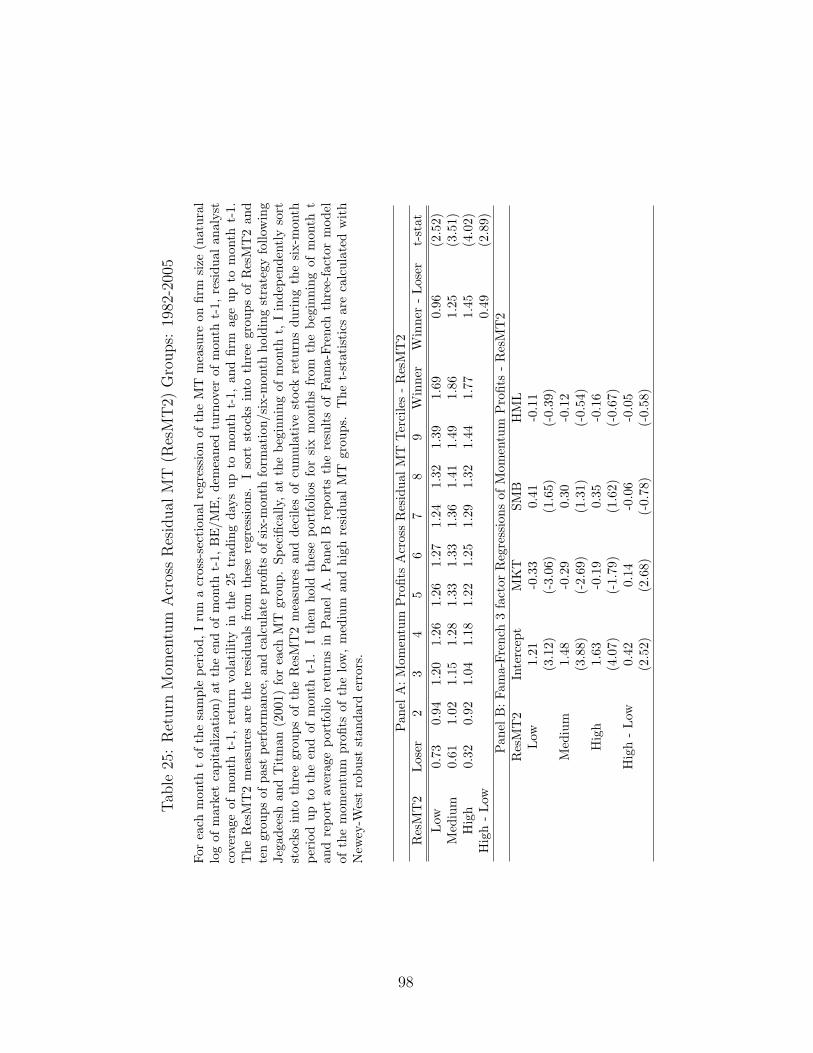
Tab

le25

:R

eturn

Mom

entu

mA

cros

sR

esid

ual

MT

(Res

MT

2)G

roups:

1982

-200

5

For

each

mon

tht

ofth

esa

mpl

epe

riod

,I

run

acr

oss-

sect

iona

lre

gres

sion

ofth

eM

Tm

easu

reon

firm

size

(nat

ural

log

ofm

arke

tca

pita

lizat

ion)

atth

een

dof

mon

tht-

1,B

E/M

E,de

mea

ned

turn

over

ofm

onth

t-1,

resi

dual

anal

yst

cove

rage

ofm

onth

t-1,

retu

rnvo

lati

lity

inth

e25

trad

ing

days

upto

mon

tht-

1,an

dfir

mag

eup

tom

onth

t-1.

The

Res

MT

2m

easu

res

are

the

resi

dual

sfr

omth

ese

regr

essi

ons.

Iso

rtst

ocks

into

thre

egr

oups

ofR

esM

T2

and

ten

grou

psof

past

perf

orm

ance

,and

calc

ulat

epr

ofits

ofsi

x-m

onth

form

atio

n/si

x-m

onth

hold

ing

stra

tegy

follo

win

gJe

gade

esh

and

Tit

man

(200

1)fo

rea

chM

Tgr

oup.

Spec

ifica

lly,at

the

begi

nnin

gof

mon

tht,

Iin

depe

nden

tly

sort

stoc

ksin

toth

ree

grou

psof

the

Res

MT

2m

easu

res

and

deci

les

ofcu

mul

ativ

est

ock

retu

rns

duri

ngth

esi

x-m

onth

peri

odup

toth

een

dof

mon

tht-

1.I

then

hold

thes

epo

rtfo

lios

for

six

mon

ths

from

the

begi

nnin

gof

mon

tht

and

repo

rtav

erag

epo

rtfo

liore

turn

sin

Pan

elA

.Pan

elB

repo

rts

the

resu

lts

ofFa

ma-

Fren

chth

ree-

fact

orm

odel

ofth

em

omen

tum

profi

tsof

the

low

,m

ediu

man

dhi

ghre

sidu

alM

Tgr

oups

.T

het-

stat

isti

csar

eca

lcul

ated

wit

hN

ewey

-Wes

tro

bust

stan

dard

erro

rs.

Pan

elA

:M

omen

tum

Pro

fits

Acr

oss

Res

idua

lM

TTer

cile

s-

Res

MT

2R

esM

T2

Los

er2

34

56

78

9W

inne

rW

inne

r-

Los

ert-

stat

Low

0.73

0.94

1.20

1.26

1.26

1.27

1.24

1.32

1.39

1.69

0.96

(2.5

2)M

ediu

m0.

611.

021.

151.

281.

331.

331.

361.

411.

491.

861.

25(3

.51)

Hig

h0.

320.

921.

041.

181.

221.

251.

291.

321.

441.

771.

45(4

.02)

Hig

h-

Low

0.49

(2.8

9)Pan

elB

:Fa

ma-

Fren

ch3

fact

orR

egre

ssio

nsof

Mom

entu

mP

rofit

s-

Res

MT

2R

esM

T2

Inte

rcep

tM

KT

SMB

HM

LLow

1.21

-0.3

30.

41-0

.11

(3.1

2)(-

3.06

)(1

.65)

(-0.

39)

Med

ium

1.48

-0.2

90.

30-0

.12

(3.8

8)(-

2.69

)(1

.31)

(-0.

54)

Hig

h1.

63-0

.19

0.35

-0.1

6(4

.07)

(-1.

79)

(1.6

2)(-

0.67

)H

igh

-Low

0.42

0.14

-0.0

6-0

.05

(2.5

2)(2

.68)

(-0.

78)

(-0.

58)

98

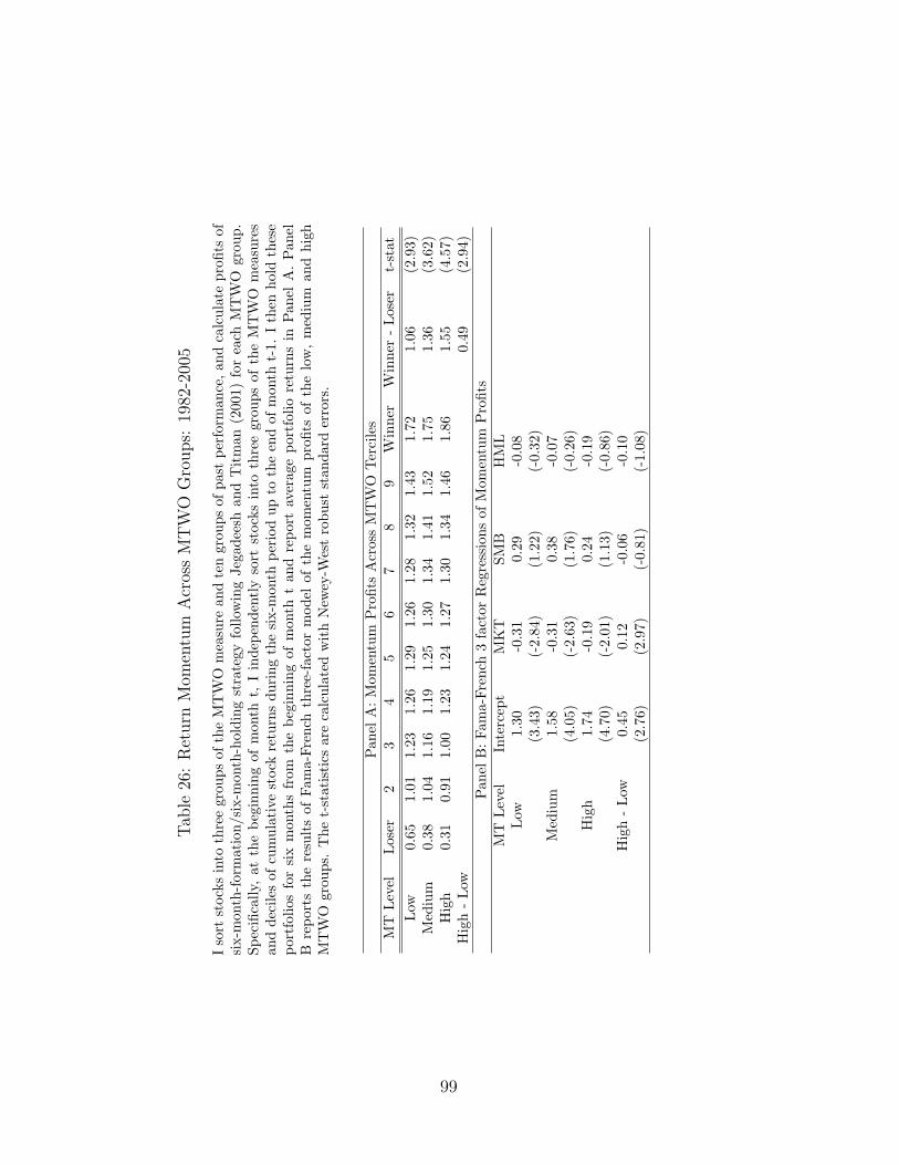
Tab

le26

:R

eturn

Mom

entu

mA

cros

sM

TW

OG

roups:

1982

-200

5

Iso

rtst

ocks

into

thre

egr

oups

ofth

eM

TW

Om

easu

rean

dte

ngr

oups

ofpa

stpe

rfor

man

ce,a

ndca

lcul

ate

profi

tsof

six-

mon

th-for

mat

ion/

six-

mon

th-h

oldi

ngst

rate

gyfo

llow

ing

Jega

dees

han

dT

itm

an(2

001)

for

each

MT

WO

grou

p.Sp

ecifi

cally

,at

the

begi

nnin

gof

mon

tht,

Iin

depe

nden

tly

sort

stoc

ksin

toth

ree

grou

psof

the

MT

WO

mea

sure

san

dde

cile

sof

cum

ulat

ive

stoc

kre

turn

sdu

ring

the

six-

mon

thpe

riod

upto

the

end

ofm

onth

t-1.

Ith

enho

ldth

ese

port

folio

sfo

rsi

xm

onth

sfr

omth

ebe

ginn

ing

ofm

onth

tan

dre

port

aver

age

port

folio

retu

rns

inPan

elA

.Pan

elB

repo

rts

the

resu

lts

ofFa

ma-

Fren

chth

ree-

fact

orm

odel

ofth

em

omen

tum

profi

tsof

the

low

,m

ediu

man

dhi

ghM

TW

Ogr

oups

.T

het-

stat

isti

csar

eca

lcul

ated

wit

hN

ewey

-Wes

tro

bust

stan

dard

erro

rs.

Pan

elA

:M

omen

tum

Pro

fits

Acr

oss

MT

WO

Ter

cile

sM

TLev

elLos

er2

34

56

78

9W

inne

rW

inne

r-

Los

ert-

stat

Low

0.65

1.01

1.23

1.26

1.29

1.26

1.28

1.32

1.43

1.72

1.06

(2.9

3)M

ediu

m0.

381.

041.

161.

191.

251.

301.

341.

411.

521.

751.

36(3

.62)

Hig

h0.

310.

911.

001.

231.

241.

271.

301.

341.

461.

861.

55(4

.57)

Hig

h-

Low

0.49

(2.9

4)Pan

elB

:Fa

ma-

Fren

ch3

fact

orR

egre

ssio

nsof

Mom

entu

mP

rofit

sM

TLev

elIn

terc

ept

MK

TSM

BH

ML

Low

1.30

-0.3

10.

29-0

.08

(3.4

3)(-

2.84

)(1

.22)

(-0.

32)

Med

ium

1.58

-0.3

10.

38-0

.07

(4.0

5)(-

2.63

)(1

.76)

(-0.

26)

Hig

h1.

74-0

.19

0.24

-0.1

9(4

.70)

(-2.

01)

(1.1

3)(-

0.86

)H

igh

-Low

0.45

0.12

-0.0

6-0

.10

(2.7

6)(2

.97)

(-0.

81)

(-1.

08)

99

Tab

le27

:E

arnin

gsR

evis

ion

Acr

oss

MT

-Mom

entu

mPor

tfol

ios:

1982

-200

5

Thi

sta

ble

repo

rtsea

rnin

gsre

visi

onsdu

ring

the

one-

year

post

-ran

king

peri

odac

ross

MT

-Mom

entu

mpo

rtfo

lios.

Ear

ning

sR

evis

ion

inm

onth

tis

the

chan

geof

the

mea

nea

rnin

gsfo

reca

sts

from

mon

tht-

1to

mon

tht,

adju

sted

byst

ock

pric

eat

the

end

ofm

onth

t-1.

At

the

begi

nnin

gof

mon

tht,

stoc

ksar

eso

rted

into

quin

tile

sof

the

MT

mea

sure

san

dpa

stsi

xm

onth

s’cu

mul

ativ

est

ock

retu

rns

(P5

refe

rsto

extr

eme

win

ner

quin

tile

and

P1

refe

rsto

extr

eme

lose

rqu

inti

le).

Nex

t,I

repo

rtin

Pan

elA

the

aver

age

earn

ings

revi

sion

sdu

ring

the

twel

vem

onth

saf

ter

port

folio

form

atio

nin

each

port

folio

and

the

diffe

renc

esbe

twee

nw

inne

rsan

dlo

sers

port

folio

sw

ithi

nM

Tqu

inti

les.

The

t-st

atis

tics

ofth

edi

ffere

nces

are

repo

rted

inpa

rent

hesi

s.Pan

elB

com

pare

sth

edi

ffere

nces

inea

rnin

gsre

visi

onbe

twee

nw

inne

rsan

dlo

sers

port

folio

sof

the

top

and

the

bott

omM

Tqu

inti

les.

The

empi

rica

lm

etho

dis

the

sam

eas

the

rolli

ngm

omen

tum

stra

tegy

exce

ptth

atI

calc

ulat

eav

erag

em

onth

lyea

rnin

gsre

visi

ons

rath

erth

anst

ock

retu

rns.

Pan

elA

:Pos

tFo

rmat

ion

Ana

lyst

sR

evis

ion

ofM

T-M

omen

tum

Por

tfol

ios

Num

ber

ofM

onth

saf

ter

Por

tfol

ioFo

rmat

ion

MT

Pas

tRet

.1

23

45

67

89

1011

12Low

P1

-0.0

252

-0.0

211

-0.0

174

-0.0

363

-0.0

228

-0.0

182

-0.0

639

-0.0

431

-0.0

476

-0.0

555

-0.0

912

-0.0

390

Low

P5

-0.0

010

-0.0

051

-0.0

065

-0.0

078

-0.0

036

-0.0

036

-0.0

041

-0.0

122

-0.0

145

-0.0

241

-0.0

115

-0.0

157

(1)

P5-

P1

0.02

420.

0160

0.01

100.

0284

0.01

920.

0146

0.05

980.

0310

0.03

310.

0313

0.07

980.

0233

t-st

at(2

.84)

(2.1

7)(1

.59)

(1.6

5)(3

.47)

(3.2

1)(2

.23)

(1.5

6)(1

.58)

(1.2

0)(1

.63)

(1.1

5)2

P1

-0.0

335

-0.0

537

-0.0

664

-0.0

522

-0.0

834

-0.0

679

-0.0

635

-0.0

470

-0.1

108

-0.0

525

-0.0

737

-0.0

626

2P

5-0

.019

2-0

.011

7-0

.009

5-0

.017

3-0

.019

8-0

.016

6-0

.005

4-0

.001

8-0

.001

9-0

.011

1-0

.015

6-0

.011

9(2

)P

5-P

10.

0142

0.04

200.

0569

0.03

490.

0636

0.05

130.

0581

0.04

510.

1089

0.04

140.

0581

0.05

08t-

stat

(0.7

1)(1

.66)

(2.5

8)(1

.64)

(2.1

4)(1

.89)

(2.7

3)(2

.22)

(2.1

8)(1

.89)

(2.0

6)(2

.03)

3P

1-0

.017

1-0

.012

9-0

.018

0-0

.013

7-0

.015

7-0

.016

8-0

.004

6-0

.020

3-0

.020

3-0

.002

90.

0037

-0.0

155

3P

5-0

.003

9-0

.010

2-0

.007

2-0

.013

0-0

.011

4-0

.007

6-0

.012

5-0

.004

7-0

.011

4-0

.003

7-0

.009

00.

0062

(3)

P5-

P1

0.01

330.

0026

0.01

080.

0008

0.00

430.

0092

-0.0

079

0.01

560.

0089

-0.0

008

-0.0

127

0.02

16t-

stat

(1.5

5)(0

.26)

(0.9

6)(0

.06)

(0.3

8)(0

.98)

(-0.

61)

(0.9

8)(0

.60)

(-0.

06)

(-0.

75)

(1.1

9)4

P1

-0.0

111

-0.0

161

-0.0

211

-0.0

224

-0.0

198

-0.0

377

-0.0

392

-0.0

252

-0.0

214

-0.0

419

-0.0

325

-0.0

187

4P

50.

0000

0.00

040.

0002

-0.0

001

0.00

010.

0002

-0.0

004

-0.0

019

-0.0

022

-0.0

023

-0.0

004

-0.0

034

(4)

P5-

P1

0.01

110.

0165

0.02

130.

0223

0.02

000.

0379

0.03

890.

0233

0.01

920.

0396

0.03

210.

0154

t-st

at(3

.34)

(2.3

1)(2

.44)

(2.9

9)(3

.44)

(2.9

0)(3

.17)

(2.9

9)(3

.19)

(2.5

4)(2

.64)

(2.7

6)H

igh

P1

-0.0

221

-0.0

164

-0.0

206

-0.0

271

-0.0

235

-0.0

265

-0.0

280

-0.0

361

-0.0

320

-0.0

386

-0.0

468

-0.0

579

Hig

hP

5-0

.000

1-0

.000

4-0

.002

2-0

.002

7-0

.002

0-0

.002

0-0

.001

4-0

.003

8-0

.002

9-0

.002

7-0

.005

1-0

.008

6(5

)P

5-P

10.

0220

0.01

610.

0184

0.02

440.

0215

0.02

450.

0267

0.03

230.

0291

0.03

590.

0416

0.04

93t-

stat

(3.7

7)(3

.66)

(3.1

0)(3

.47)

(4.3

7)(4

.29)

(3.8

6)(2

.75)

(3.0

0)(3

.50)

(2.6

8)(2

.42)

Pan

elB

:C

ompa

riso

nof

Diff

eren

ces

inA

naly

stFo

reca

sts

(5)

-(1

)-0

.002

20.

0001

0.00

74-0

.004

00.

0023

0.00

99-0

.033

20.

0013

-0.0

041

0.00

46-0

.038

10.

0260

t-st

at(-

0.21

)(0

.01)

(0.8

2)(-

0.22

)(0

.31)

(1.3

5)(-

1.19

)(0

.06)

(-0.

18)

(0.1

6)(-

0.74

)(0

.90)

100

Tab

le28

:Lon

g-Ter

mR

ever

sals

inM

omen

tum

Pro

fits

Acr

oss

MT

Lev

els

At

the

begi

nnin

gof

mon

tht,

Iin

depe

nden

tly

sort

stoc

ksin

toqu

inti

les

ofth

eM

Tm

easu

res

and

past

six

mon

ths’

cum

ulat

ive

stoc

kre

turn

s.I

then

calc

ulat

ew

ithi

nea

chM

Tqu

inti

leth

ecu

mul

ativ

em

omen

tum

profi

ts(t

oppa

st-r

etur

nqu

inti

lem

inus

bott

ompa

st-r

etur

nqu

inti

le)

upto

each

mon

thdu

ring

the

thre

e-ye

arpo

st-r

anki

ngpe

riod

.R

etur

nsar

em

easu

red

inth

esc

ale

ofpe

rcen

tage

.

Num

ber

ofM

onth

sA

fter

Por

tfol

ioFo

rmat

ion

MT

36

912

1518

2124

2730

3336

36-1

2Low

2.17

4.34

6.69

7.14

5.21

4.13

4.29

3.92

2.70

2.41

3.42

3.70

-3.4

42

1.67

4.15

7.09

7.58

6.45

6.07

6.33

6.13

3.94

3.38

4.01

3.79

-3.7

93

1.77

4.72

7.15

7.78

6.98

6.54

6.63

5.91

4.32

3.98

4.24

4.03

-3.7

54

2.53

5.80

8.86

9.68

8.68

8.26

8.55

7.62

5.58

4.81

5.35

4.85

-4.8

3H

igh

3.47

7.39

10.0

811

.18

10.2

79.

149.

458.

706.

976.

095.

414.

82-6

.36

101

Table 29: Six-Month/Six-Month Strategy: Two-Dimensional Sort on FITand MT: 1982-2005

This table presents momentum profits across FIT-MT groups. At the beginning of month t, I indepen-dently sort stocks into three groups of the MT measures, three groups of one-quarter lag FIT measures,and quintiles of cumulative returns over the six-month period up to the end of month t-1. Following thesix-month holding/six-month formation strategy of Jegadeesh and Titman (2001), I hold these three-dimensionally sorted portfolios for six months. Panel A reports the average monthly returns of theportfolios and Panel B reports the comparisons of momentum profits across the FIT-MT groups.

Panel A: Momentum Profits across FIT-Inst.Ownership groupsFIT MT Loser 2 3 4 Winner W - L t-statLow Low 0.74 1.08 1.07 1.07 1.36 0.62 (2.68)Low Med 0.76 1.07 1.18 1.19 1.59 0.83 (3.46)Low High 0.58 1.01 1.15 1.22 1.78 1.21 (5.06)

2 Low 1.15 1.33 1.35 1.27 1.46 0.32 (1.56)2 Med 1.10 1.34 1.46 1.36 1.52 0.42 (2.16)2 High 0.96 1.35 1.42 1.40 1.55 0.59 (2.80)

High Low 1.27 1.31 1.32 1.32 1.47 0.20 (1.08)High Med 1.23 1.44 1.41 1.43 1.58 0.35 (2.00)High High 1.22 1.44 1.48 1.48 1.76 0.53 (2.90)

Panel B: Matrix of Momentum ProfitsFIT Level

Low Med. High L-H t-statLow 0.62 0.32 0.20 0.42 (2.42)

MT Level Med. 0.83 0.42 0.35 0.48 (2.65)High 1.21 0.59 0.53 0.67 (3.89)H-L 0.58 0.27 0.33

t-stat (3.27) (1.77) (2.22)

102

References

Alangar, Sadhana, Chenchuramaiah T. Bathala, and Ramesh P. Rao, 1999,

The effect of institutional interest on the information content of dividend-

change announcements, Journal of Financial Research 22, 429–448.

Almazan, Andres, Keith C. Brown, Murray Carlson, and David A. Chapman,

2004, Why constrain your mutual fund manager, Journal of Financial

Economics 73, 289–321.

Amihud, Yakov, 2002, Illiquidity and stock returns: Cross-section and time-

series effects, Journal of Financial Markets 5, 31–56.

Andreassen, Paul B., and Stephen J. Kraus, 1990, Judgemental extrapolation

and the salience of change, Journal of Forecasting 9, 347–372.

Asquith, Paul, Parag A. Pathak, and Jay R. Ritter, 2005, Short interest,

institutional ownership, and stock returns, Journal of Financial Economics

78, 243–276.

Badrinath, S. G., and Sunil Wahal, 2002, Momentum trading by institutions,

Journal of Finance 57, 2449–2478.

Baks, Klaas P., Andrew Metrick, and Jessica Wachter, 2001, Should investors

avoid all actively managed mutual funds? a study in bayesian performance

evaluation, Journal of Finance 56, 45–85.

Bartov, Eli, Suresh Radhakrishnan, and Itzhak Krinsky, 2000, Investor so-

phistication and patterns in stock returns after earnings announcements,

Accounting Review 75, 43–63.

Bennett, James A., Richard W. Sias, and Laura T. Starks, 2003, Greener

pastures and the impact of dynamic institutional preferences, Review of

Financial Studies 16, 1203–1238.

Boehmer, Ekkehart, and Eric Kelley, 2006, Institutional investors and infor-

mation efficiency of prices, Working Paper, Texas A & M University.

Bollen, Nicolas P. B., and Jeffrey A. Busse, 2001, On the timing ability of

mutual fund managers, Journal of Finance 56, 1075–1095.

103

Brown, Stephen J., William N. Goetzmann, Roger G. Ibbotson, and

Stephen A. Ross, 1992, Survivorship bias in performance studies, Review

of Financial Studies 5, 553–580.

Brunnermeier, Markus K., and Stefan Nagel, 2004, Hedge funds and the

technology bubble, Journal of Finance 59, 2013–2040.

Bushee, Brian J., 1998, The influence of institutional investors in myopic

R&D investment behavior, Accounting Review 73, 305–333.

, 2001, Do institutional investors prefer near-term earnings over long-

run value?, Contemporary Accounting Research 2, 207–246.

Carhart, Mark M., 1997, On persistence in mutual fund performance, Journal

of Finance 52, 57–82.

, Jennifer N. Carpenter, Anthony W. Lynch, and David K. Musto,

2002, Mutual fund survivorship, Review of Financial Studies 15, 1439–

1463.

Chakravarty, Sugato, 2001, Stealth-trading: Which traders’ trades move

stock prices?, Journal of Financial Economics 61, 289–307.

Chan, Louis K.C, Narasimhan Jegadeesh, and Josef Lakonishok, 1996, Mo-

mentum strategies, Journal of Finance 51, 1681–1713.

Chan, Louis K.C, and Josef Lakonishok, 1995, The behavior of stock prices

around institutional trades, Journal of Finance 50, 1147–1174.

, 1997, Institutional equity trading costs: NYSE versus Nasdaq, Jour-

nal of Finance 52, 713–735.

Chen, Hsiu-Lang, Narasimhan Jegadeesh, and Russ Wermers, 2000, The

value of active mutual fund management: An examination of the stock-

holdings and trades of fund managers, Journal of Financial and Quanti-

tative Analysis 35, 343–368.

Chen, Joseph, Harrison Hong, and Jeremy C. Stein, 2002, Breadth of own-

ership and stock returns, Journal of Financial Economics 66, 171–205.

Cohen, Randolph, Paul A. Gompers, and Tuomo Vuolteenaho, 2002, Who

underreacts to cash-flow news? Evidence from trading between individuals

and institutions, Journal of Financial Economics 66, 409–462.

104

Cohen, Randolph B., Joshua D. Coval, and Lubos Pastor, 2005, Judging fund

managers by the company they keep, Journal of Finance 60, 1057–1096.

Collins, Daniel W., Guojin Gong, and Paul Hribar, 2003, Investor sophis-

tication and the mispricing of accruals, Review of Accounting Studies 8,

251–276.

Dahlquist, Magnus, and Goran Robertsson, 2001, Direct foreign ownership,

institutional investors, and firm characteristics, Journal of Financial Eco-

nomics 59, 413–440.

Dahlquist, Magnus, and Paul Soderlind, 1999, Evaluating portfolio perfor-

mance with stochastic discount factors, Journal of Business 72, 347–383.

Daniel, Kent, Mark Grinblatt, Sheridan Titman, and Russ Wermers, 1997,

Measuring mutual fund performance with characteristic-based bench-

marks, Journal of Finance 52, 1035–1058.

Daniel, Kent, and Sheridan Titman, 1997, Evidence on the characteristics of

cross-sectional variation in stock returns, Journal of Finance 52, 1–33.

, 1999, Market efficiency in an irrational world, Financial Analysts

Journal 55, 28–40.

Del Guercio, Diane, 1996, The distorting effect of the prudent-man laws on

institutional equity investments, Journal of Financial Economics 40, 31–

62.

DeLong, Bradford J., Andrei Shleifer, Lawrence H. Summers, and Robert J.

Waldmann, 1990a, Noise trader risk in financial market, Journal of Polit-

ical Economy 98, 703–738.

, 1990b, Positive feedback investment strategies and destabilizing

rational speculation, Journal of Finance 45, 379–395.

Falkenstein, Eric G., 1996, Preferences for stock characteristics as revealed

by mutual fund portfolio holdings, Journal of Finance 51, 111–135.

Fama, Eugene F., and Kenneth R. French, 1992, The cross-section of ex-

pected stock returns, Journal of Finance 47, 427–466.

Ferson, Wayne E., and Rudi W. Schadt, 1996, Measuring fund strategy and

performance in changing economic conditions, Journal of Finance 51, 425–

461.

105

Frazzini, Andrea, 2005, The disposition effect and underreaction to news,

Journal of Finance Forthcoming.

Froot, Kenneth A., David S. Scharfstein, and Jeremy C. Stein, 1992, Herd

on the street: Informational inefficiencies in a market with short-term

speculation, Journal of Finance 47, 1461–1484.

Geczy, Christopher C., David K. Musto, and Adam V. Reed, 2002, Stocks are

special too: An analysis of the equity lending market, Journal of Financial

Economics 66, 241–269.

Gillan, Stuart L., and Laura T. Starks, 2000, Corporate governance proposals

and shareholder activism: The role of institutional investors, Journal of

Financial Economics 57, 275–305.

Gompers, Paul A., and Andrew Metrick, 2001, Institutional investors and

equity prices, Quarterly Journal of Economics 116, 229–259.

Griffin, John M., Jeffrey H. Harris, and Selim Topaloglu, 2003, The dynamics

of institutional and individual trading, Journal of Finance 58, 2285–2320.

Griffin, John. M., and Mark L. Lemmon, 2002, Book-to-market equity, dis-

tress risk, and stock returns, Journal of Finance 57, 2317–2336.

Grinblatt, Mark, and Matti Keloharju, 2000, The investment behavior and

performance of various investor types: A study of Finland’s unique data

set, Journal of Financial Economics 55, 43–67.

Grinblatt, Mark, and Sheridan Titman, 1992, The persistence of mutual fund

performance, Journal of Finance 47, 1977–1984.

, 1993, Performance measurement without benchmarks: An exami-

nation of mutual fund returns, Journal of Business 66, 47–68.

, 1994, A study of monthly mutual fund returns and performance

evaluation techniques, Journal of Financial and Quantitative Analysis 29,

419–444.

, and Russ Wermers, 1995, Momentum investment strategies, portfo-

lio performance, and herding: A study of mutual fund behavior, American

Economic Review 85, 1088–1105.

106

Grinstein, Yaniv, and Roni Michaely, 2005, Institutional holdings and payout

policy, Journal of Finance 60, 1389–1426.

Han, Bin, and Qinghai Wang, 2005, Institutional investors, investment con-

straints and stock momentum, Working Paper, Ohio State University.

Hartzell, Jay C., and Laura T. Starks, 2003, Institutional investors and ex-

ecutive compensation, Journal of Finance 58, 2351–2374.

Hasbrouck, Joel, 1993, Assessing the quality of a security market: A new

approach to transaction-cost measurement, Review of Financial Studies 6,

191–212.

, 2006, Trading costs and returns for us equities: The evidence from

daily data, Working Paper, New York University.

Hirshleifer, David A., Avanidhar Subrahmanyam, and Sheridan Titman,

1994, Security analysis and trading patterns when some investors receive

information before others, Journal of Finance 49, 1665–1698.

Holden, Craig W., and Avanidhar Subrahmanyam, 1992, Long-lived private

information and imperfect competition, Journal of Finance 47, 247–270.

Hong, Dong, Charles M.C. Lee, and Bhaskaran Swaminathan, 2003, Earnings

momentum in international markets, Working Paper, Cornell University.

Hong, Harrison, Terence Lim, and Jeremy C. Stein, 2000, Bad news travels

slowly: Size, analyst coverage, and the profitability of momentum strate-

gies, Journal of Finance 55, 265–295.

Hong, Harrison, and Jeremy C. Stein, 1999, A unified theory of underreac-

tion, momentum trading, and overreaction in asset markets, Journal of

Finance 54, 2143–2184.

Irvine, Paul, Marc Lipson, and Andy Puckett, 2007, Tipping, Journal of

Finance , forthcoming.

Jegadeesh, Narasimhan, and Sheridan Titman, 1993, Returns to buying win-

ners and selling losers: Implications for stock market efficiency, Journal of

Finance 48, 65–91.

, 2001, Profitability of momentum strategies: An evaluation of alter-

native explanations, Journal of Finance 56, 699–720.

107

Jiang, Guohua, Charles M. C. Lee, and Yi Zhang, 2005, Information uncer-

tainty and expected returns, Review of Accounting Studies 10, 185–221.

Lakonishok, Josef, Armun Shleifer, Richard Thaler, and Robert W. Vishny,

1991, Window dressing by pension fund managers, American Economic

Review 81, 227–231.

Lakonishok, Josef, Andrei Shleifer, and Robert W. Vishny, 1992, The impact

of institutional trading on stock prices, Journal of Financial Economics

32, 23–43.

, 1994, Contrarian investment, extrapolation, and risk, Journal of

Finance 49, 1541–1578.

Lee, Charles M.C., and Bhaskaran Swaminthan, 2000, Price momentum and

trading volume, Journal of Finance 55, 2017–2069.

Malkiel, Burton G., 1995, Returns from investing in equity mutual funds

1971 to 1991, Journal of Finance 50, 549–572.

Nagel, Stefan, 2005, Short sales, institutional investors and the cross-section

of stock returns, Journal of Financial Economics 78, 277–309.

Ng, Lilian, and Qinghai Wang, 2004, Institutional trading and the turn-of-

the-year effect, Journal of Financial Economics 74, 343–366.

Nofsinger, John R., and Richard W. Sias, 1999, Herding and feedback trading

by institutional and individual investors, Journal of Finance 54, 2263–

2295.

Odean, Terrance, 1999, Do investors trade too much?, American Economic

Review 89, 1279–1298.

Parrino, Robert, Richard W. Sias, and Laura T. Starks, 2003, Voting with

their feet: Institutional ownership changes around forced CEO turnover,

Journal of Financial Economics 68, 3–46.

Pastor, Lubos, and Robert F. Stambaugh, 2002a, Investing in equity mutual

funds, Journal of Financial Economics 63, 351–380.

, 2002b, Mutual fund performance and seemingly unrelated assets,

Journal of Financial Economics 63, 315–349.

108

Shleifer, Andrei, and Robert W. Vishny, 1997, The limits of arbitrage, Jour-

nal of Finance 52, 35–55.

Sias, Richard W., 2004, Institutional herding, Review of Financial Studies

17, 165–206.

, and Laura T. Starks, 1997, Institutions and individuals at the turn-

of-the-year, Journal of Finance 52, 1543–1562.

, and Sheridan Titman, 2006, Changes in institutional ownership and

stock returns: Assessment and methodology, Journal of Business.

Wermers, Russ, 1999, Mutual fund herding and the impact on stock prices,

Journal of Finance 54, 581–622.

, 2000, Mutual fund performance: An empirical decomposition into

stock-picking talent, style, transaction costs and expenses, Journal of Fi-

nance 55, 1655–1695.

Zhang, Frank, 2006, Information uncertainty and stock returns, Journal of

Finance 61, 105–136.

Zhang, Lu, 2005, The value premium, Journal of Finance 60, 67–103.

109

VITA

Tao Shu was born in Wuhan City, China on July 2, 1975, the son of

Quanmei Jiang and Huizhi Shu. After completing his work at Wuhan

Foreign Language School, Wuhan City, China, in 1993, he entered the

Zhongnan University of Finance and Economics in Wuhan City, China. He

received the degree of Bachelor of Economics from Zhongnan University of

Finance and Economics in July 1997. During the following years he was

employed as a financial analyst at China Development Bank, Xiamen,

China. In September 2001 he entered the Graduate School of The University

of Texas as a Master student in Statistics. He received the degree of Master

of Science in Statistics from the University of Texas at Austin in August

2003. In September 2003 he entered the Doctoral Program in Finance at the

University of Texas at Austin.

Permanent Address: 2501 Lake Austin Blvd Apt E110, Austin TX 78703

This dissertation was typed by the author

110