Copyright by Sudip Chakraborty 2016

Copyright

by

SudipChakraborty

2016

TheDissertationCommitteeforSudipChakrabortyCertifiesthatthisisthe

approvedversionofthefollowingdissertation:

InteractionbetweenAerosolsandtheMesoscaleConvectiveSystemsover

theTropicalContinents

Committee:

RongFu,Supervisor

RobertE.Dickinson

Zong‐LiangYang

DavidT.Allen

StevenT.Massie

JoseMarengo



by

SudipChakraborty,B.E.;M.Tech

Dissertation

PresentedtotheFacultyoftheGraduateSchoolof

TheUniversityofTexasatAustin

inPartialFulfillment

oftheRequirements

fortheDegreeof

DoctorofPhilosophy

TheUniversityofTexasatAustin

May2016

Dedication

To,

Rik

v

Acknowledgements

There would be no words that can thank my supervisor Dr. Rong Fu

enough.MydreamofhighereducationandpursuingaPh.D.wouldnothavebeen

possiblehadtherebeennosupportandtheletterofacceptancefromherwhenI

was in India.She isagreatsupervisor.She taughtme thescientificknowledge,

writing, and helped improving my research skills. Her instructions and the

courses she taught have shown me the road map to be a scientist from an

undergraduatestudent.Thetransitionfromanundergradtoascientistfounda

responsible, caring, and innovative hands of Rong. Not only she is a great

inspirationandenthusiasticsupervisortome,herfriendlynaturehashelpedme

a lot in difficult and tough times in life. Her supportive and warm‐hearted

supervisionhavealwayshelpedmetobeconfidentinresearchduringmydegree

requirementsandachievingmy futuregoals.Shehasalwaysencouragedmeto

work in the researchofmychoiceand Iam fortunate that Iwouldcontinue to

workwithheraftermygraduation.

Itwouldhavebeenimpossiblewithoutmythreeyear’soldlittledaughter,

Sharanya,whoseinnocent,cute,beautifulsmiles,andlovearethebiggestsources

ofenergyandenthusiasmforme.SheisthereasonIfeelresponsible,caring,and

dedicated tomy family andwork. It’s her love that showsme the steps in the

future.Shemakesmefeeltheimportanceofmylife.

Iwantto thankDr.StevenT.Massie forhisgreatsupportandguidance

for the progress of my research projects and the knowledge he shared to

improvemymanuscriptsandscientificwriting.

Thanks to my parents and Monalisa. It would have been impossible

withoutthebasicknowledgeofeverythingtheytaughtmeandthecourageand

supporttheygaveme.ThankstoallmyprofessorsinUTAustinforshowingme

vi

thepathwayofbeingascientistbyenrichingmyknowledgeandencouragingme

toaskquestions,whichisimmenselyimportanttobeingascientist.

Thanks to Dr. Jonathon S. Wright and Dr. Graeme Stephens for their

insightful contributions to our publications. I acknowledge my dissertation

committeemembers, Drs. Robert E. Dickinson, Zong‐Liang Yang, and David T.

Allenfortheirimportantfeedbackduringmydefenseprocess.

IalsoacknowledgemyresearchgroupmembersinUTAustin.Ithasbeen

a pleasure to workwith all of them. Thanks tomy friends from different and

diverseresearchgroupsintheJacksonSchoolofGeosciencesatUTAustin.They

havemademylifemuchhappierandeasier!

vii



SudipChakraborty,Ph.D.

TheUniversityofTexasatAustin,2016

Supervisor:RongFu

Abstract

Presence of aerosols in the upper troposphere can have significant

impacts on the Earth’s radiative energy budget. However, the aerosol–cloud

relationship represents the largest uncertainty in the radiative energy budget.

Relationships between aerosols and themesoscale convective systems (MCSs)

are complicated and difficult to ascertain, due in large part to inadequate

availability of satellite datasets until recent years. Variation of aerosol impacts

withmeteorologicalparameters and the relative influenceof theseparameters

on the convective strength of the MSCs can also be attributed to limited

detectabilityofaerosol invigorationeffects.Toaddressthe interactionbetween

aerosolandtheMCSs,IfirstaddresstheinfluenceofMCSonthedistributionof

the aerosols,which is poorly known on a global scale. Then, I investigate the

influence of aerosol on MCSs. This dissertation addresses these problems by

collocatingasuiteofgeostationaryandpolarorbitalsatellitesatthreedifferent

phases of their convective lifecycle. First, I estimate the extent of upper

viii

tropospheric aerosol layers (UT ALs) surrounding the MCSs and explore the

relationships between UT AL extent and the morphology, location, and

developmental stages of collocatedMCSs in the tropics over equatorialAfrica,

SouthAsia,andtheAmazonbasinbetweenJune2006andJune2008. I identify

that themost extensive UT ALs over equatorial Africa are associatedwith the

matureMCSs,whilethemostextensiveUTALsoverSouthAsiaandtheAmazon

basinareassociatedwith thegrowingMCSs.Convectiveaerosol transportover

Amazonia is weaker than that observed over the other two regions despite

similar transport frequencies, likely due to smaller sizes and shorter mean

lifetimesofAmazonianMCSs.VariationsinUTALsinthevicinityoftropicalMCSs

are primarily explained by variations in the horizontal sizes of the associated

MCSs and are not related to aerosol loading in the lower troposphere.

Relationshipsbetweenconvectivepropertiesandaerosoltransportarerelatively

weakduringthedecayingstageofconvectivedevelopment.

Then I estimate the relative influence of aerosols and other

meteorological parameters on MCS strength and longevity using collocated

samplesofMCSsfromJanuary2003toJune2008.Theresultsshowthatrelative

humidity (RH) and convective available potential energy (CAPE) have the

strongestimpactsonMCSlifetimeandenhancethelifetimeoftheMCSsby6‐36

hourswhenother parameters such as verticalwind shear (VWS) and aerosols

are kept constant. Aerosols also enhance the convective lifetime of MCSs,

howeverat amuchweaker rate (6‐24h)andonlywhenRHandVWSarehigh.

Moreover,aerosolinfluenceonconvectivelifetimeisdetectedduringthemature

anddecayingphasesonly.At the continental scale, aerosolsexplain20‐27%of

ix

the total variance ofMCSs’ lifetimeover equatorial SouthAmerica, but explain

only8%ofthesameoverequatorialAfrica.SouthAsianMCSsaremorestrongly

influenced by meteorological parameters and MCS‐associated aerosols when

they are over the ocean than when over the land since most MCSs form and

developovertheoceans.

After that, I estimate the influence of aerosols and other meteorological

parameters onMCSs’ rain rate (RR). Results show that an increase in aerosol

concentrationenhanceIWCandsuppressRRandLHduringall threephasesof

convectivelifetime.IncreasingaerosolconcentrationssuppressRRattherateof

‐0.38mm/hand‐0.47mm/hduringthegrowing,decayingphaseswhenVWSis

high and at a rate of ‐0.30 mm/h during the mature phase when RH is low.

MeteorologicalparameterssuchasVWSandRHhavesignificanteffectsonthese

aerosol influences.The suppressionofRR is alsoassociatedwithadecrease in

latent heat released by large hydrometeors. Aerosols explain 16%, 23%, and

29% of RR’s variance during the growing, mature and decaying phases,

respectively,asestimatedbyamultiplelinearregressionmethod.Consequently,

aerosolsenhanceIWCoftheMCSsinsidetheanvilupto0.72,1.41,0.82mg/m3

andenhancethetotalintegratedreflectivityofthelarger‐sizediceparticlesupto

8,11,and18dBZintheconvectivecoreregionsduringthegrowing,matureand

decayingphases, respectively. In contrast, changes (one standarddeviation) in

CAPEandRHenhancetheRRupto0.35mm/h.

This dissertation study provides the first satellite based global tropical

assessmentof the relative influencesofaerosolsandmeteorological conditions

on MCSs’ lifetime, rain rate, and IWC and the mutual dependence of these

x

influences. It also shows how aerosols influence the rain rate, cloud ice and

lifetimeoftheMCSs,varyingwithintheirlifecycleandbetweendifferenttropical

continentsrangingfromhumidequatorialSouthAmericaduringwetseasonand

bigmonsoonal systemsoverSouthAsia to relativelydryequatorialAfricawith

highaerosol loading. Indoingso, thisworkhasalsoadvancedourcapability to

evaluate whether or not aerosols could increase convective lifetime by

suppressing rain rateand invigorating theMCSsonclimatescaleandwhatare

the favorablemeteorological conditions for aerosol to affect the lifetimeof the

MCSs. Our results also provide an interpretive framework for devising and

evaluating numerical model experiments that can examine relationships

betweenconvectivepropertiesandALstransportedintheuppertroposphere.In

thefuture,wewouldliketoinvestigatetheinfluenceofdifferentmeteorological

parameters and aerosols on extra tropical MCSs and on self‐aggregation of

convection.

.

xi

TableofContents

Abstract .................................................................................................................................. vii

ListofTables ......................................................................................................................... xiii

ListofFigures ....................................................................................................................... xiv

Chapter1 .................................................................................................................................. 1

GeneralIntroduction ............................................................................................................. 1

Chapter2 ................................................................................................................................ 11

Relationshipsbetweenconvectivestructureandtransportofaerosolstotheuppertropospherededucedfromsatelliteobservations ............................................ 11

2.1Introduction .................................................................................................................... 11

2.2.DataandMethodology ................................................................................................. 15

2.2.1.Identificationanddescriptionofcloudsandaerosollayers ............................. 15

2.2.2.Data ............................................................................................................................... 17

2.2.3.Collocationcriteria .................................................................................................... 24

2.2.4.Statisticalmodelconstruction ................................................................................ 31

2.3Results .............................................................................................................................. 35

2.4.Statisticalmodelresultsanddiscussion .................................................................. 42

2.5.Summary ......................................................................................................................... 54

Chapter3 ................................................................................................................................ 59

Relativeinfluenceofthemeteorologicalconditionsandaerosolsonthelifetimeofthemesoscaleconvectivesystems .................................................................................... 59

3.1Introduction .................................................................................................................... 59

3.2DataandMethods .......................................................................................................... 63

3.3ResultsandDiscussion.................................................................................................. 64

3.4SupportingInformation ................................................................................................ 80

3.4.1Data ................................................................................................................................ 80

3.4.2Statisticalmethods ..................................................................................................... 84

Chapter4 ................................................................................................................................ 90

Relativeinfluenceofthemeteorologicalandaerosolconditionsonthemesoscaleconvectivesystemsthroughtheirlifecycleovertropicalcontinents ........................ 90

4.1.Introduction ................................................................................................................... 90

4.2 DataandMethodology ................................................................................................. 94

4.2.1 Data ................................................................................................................................ 94

xii

4.2.2 Methodology ................................................................................................................ 97

4.2.3 Statisticalmethods ................................................................................................... 101

4.3 Results ............................................................................................................................ 102

4.4 Conclusion ..................................................................................................................... 113

Chapter5 .............................................................................................................................. 116

GeneralConclusions ........................................................................................................... 116

References ............................................................................................................................ 124

xiii

ListofTables

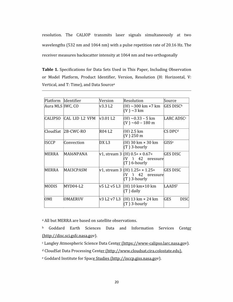
Table1.Specifications forDataSetsUsed inThisPaper, IncludingObservation

or Model Platform, Product Identifier, Version, Resolution (H: Horizontal, V:

Vertical,andT:Time),andDataSourcea................................................................................20

Table2.Coefficientsforbackground‐relativeaerosolpixelcountsbetween4and

20km in optimal statistical models by stage of convective development, along

withthecorrelationcoefficientbetweentheexpectedandpredictedvaluesinthe

testdata(R2)andtheexplainedvarianceinthetestdata(EV)...................................45


20kminoptimalstatisticalmodelsbyregiona....................................................................46

xiv

ListofFigures

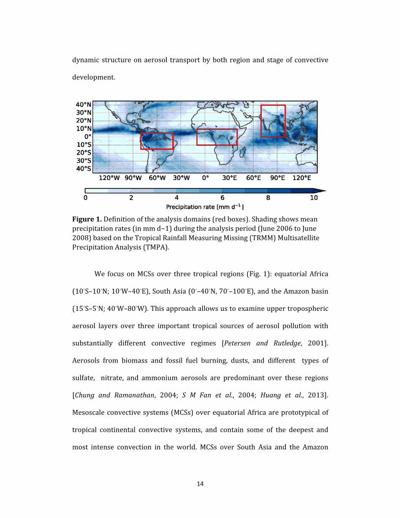
Figure1.Definitionoftheanalysisdomains(redboxes).Shadingshowsmeanprecipitationrates(inmmd−1)duringtheanalysisperiod(June2006toJune2008)basedontheTropicalRainfallMeasuringMissing(TRMM)MultisatellitePrecipitationAnalysis(TMPA). ..................................................................................................................... 14

Figure2.AnexampleofacollocatedMCS,including(a)theoriginanddevelopmentoftheMCS,(b)theverticaldistributionofIWCandfractionalCOanomaliesintheuppertropospherealongtheMLStrack,and(c)theverticaldistributionofaerosolandcloudlayersalongtheCALIPSOandCloudSattrack.ThisMCSwasfirstdetectedbyISCCPat21UTC20January2007at16.7∘Sand57.3∘W.Thesystemthenmovedwest,wheretheA‐Trainsatellitesobserveditatapproximately06UTC21January.ThedarkandlightbluecirclesinFigure2ashowtheapproximatecentralpositionandradiusoftheMCSattheA‐Trainoverpasstime.ThecloudwasgrowingwhenCALIPSOandCloudSat(redline)observeditstrailingedgeat05:27UTCandAuraMLS(greenline)observedthesystemnearitscenterat05:35UTC.Thecentralpositionsofeachsatellitefootprintareshownaswhitecirclesalongthesatellitetrack. .............................................................................. 34

Figure3.Boxandwhiskerplotsshowingthedistributionsoftheheightoftheaerosollayer(HAL),theheightofmaximumconvectivedetrainment(HDL),andthecloudtopheight(CTH)forcollocatedMCSs.Thebottomandtopofeachboxrepresenttheupperandlowerquartiles,respectively,andthehorizontallineinsidetheboxrepresentsthemedian.Theendsofthewhiskersaretheminimumandmaximumofthedata.MCSswithHAL<6km(theminimumobserveddetrainmentlayer)havebeenexcluded. ....... 36

Figure4.Meanprofilesof(a)IWCand(b)COintheuppertropospherebasedonAuraMLSprofilescollocatedwithgrowing(red),mature(purple),anddecaying(blue)MCSs.Shadingrepresentsintervalsofonestandarderroraroundthemean. ............................. 37

Figure5.Variationsinmeanvaluesof(a)verticallyintegratedanomalyinnumberofaerosolpixels,(b)aerosollayerheight(HAL),(c)stormradius,(d)cloudtopheight(CTH),(e)numberofconvectivecores(NCC),(f)convectivefraction(CF),and(g)precipitationrateduringdifferentstagesoftheconvectivelifecycle.Errorbarsandshadingrepresentintervalsoftwostandarderrorsaroundthemean. ............................. 38

Figure6.Verticalprofilesofaerosoltransportassociatedwithgrowing(red),mature(purple),decaying(blue),andshort‐livedconvectiveevents(gray)over(a)equatorialAfrica,(b)SouthAsia,and(c)theAmazonbasin.Theleftsideofeachpanelshowstheverticaldistributionofthefractionofconvectiveeventsforwhichtheanomalyinaerosolpixelsrelativetothebackgroundprofileispositive.Therightsideofeachpanelshowsthemeananomalyinthenumberofaerosolpixelsatthatheight.Theverticalresolutionis2km.Errorbarsindicateintervalsofonestandarderroraroundthemean. .................................................................................................................................................. 40

Figure7.Fractionofvarianceofaerosollayerextentinthebinneddataexplainedbytheindependentvariablesintheoptimalstatisticalmodelsforaerosoltransportassociated

xv

with(a)allMCSs,(b)growingMCSs,(c)matureMCSs,and(d)decayingMCSs.Grayareashowsfractionofvariancenotexplained. ............................................................................ 43

Figure8.Scattermatrixshowingco‐variabilityamongtheindependentvariables(ordinatesinfirsttothirdrows;abscissasinfirsttothirdcolumns)andthedependentvariable(ordinateinfourthrow;abscissainfourthcolumn)intheoptimalstatisticalmodelforaerosoltransportassociatedwithallMCSs.Themodel‐independentvariables(intheorderofimportance)areradius,numberofconvectivecores(NCC),andverticalwindshear(VWS).Thedependentvariableistheverticallyintegratedanomalyinaerosolpixels(seetextfordetails).Redlinesinscatterplotsshowlinearrelationships;bluelinesshowlocallinearregressionsusingalowessfilter.Bluecurvesalongthediagonalshowthedensitydistributionsofeachvariable(scaleasshowninthetopleftordinate). ................................................................................................................................. 47

Figure9.AsinFigure8,butforgrowingMCSs.Theindependentvariablesareradiusandverticalwindshear(VWS). ............................................................................................. 48

Figure10.AsinFigure8,butformatureMCSs.Theindependentvariablesareradius,numberofconvectivecores(NCC),andconvectivefraction(CF). ..................................... 49

Figure11.AsinFigure8,butfordecayingMCSs.Theindependentvariablesareradiusandaerosolopticaldepth(AOD). .......................................................................................... 50

Figure12.Graphicalrepresentationsofthestatisticalmodelsfor(a)allMCSs,(b)growingMCSs,(c)matureMCSs,and(d)decayingMCSs.ThemodelsforallMCSsandmatureMCSshavebeencollapsedintotwodimensionsbyusingthestronglinearcorrelationbetweenradiusandNCC(seetextandFigures8and10).Ascatterplotofthebinneddataforeachcaseisshownforreference,andthefractionofvarianceexplainedbythelinearmodelisshownatthetoprightofeachpanel. ............................................... 54

Figure13.TherateofchangeofMCSs’lifetime(hours,colorshades)with(a)CAPE,(b)RH850,(c)RH500asafunctionoffAODusingAOD>0.15overlandandAOD>0.3overtheoceanasthethresholdforapollutedenvironmentandthedeeptroposphericVWS,(d)fAODasafunctionofRH850andthedeeptroposphericVWS,(e)fAODasafunctionofCAPEandthedeeptroposphericVWS,and(f)VWSasafunctionoftheRH850andfAOD.TheratesrepresentachangeofMCSs'lifetimeinhoursassociatedwiththevariationof1σofthatparameter.Thebinswiththenumberofsampleslessthan20andinsignificantrateofchangeat95%confidencelevelarenotshown.Note:fAOD=NPAOD>0.15/(NPAOD>0.15+NPAOD<0.15)overlandandfAOD=NPAOD>0.30/(NPAOD>0.30+NPAOD<0.30)overocean.NPisthenumberofpixels.Thepiechartin(f)showsthefractionofvarianceofMCS’slifetimeexplainedbytheenvironmentalvariablesusingmultiplelinearregressionforalltheMCSs. ........................................................................................................................................ 77

Figure14.FractionofthetotalvarianceoftheMCS’slifetime(a,b,c),IZ(d,e,f),andIWC_216(g,h,i)explainedbytheenvironmentalvariablesbasedonthemultiplelinearregressionduringthegrowing,mature,anddecayingphasesoftheMCSs. ...................... 78

Figure15.FractionofthetotalvarianceofMCS’slifetimeoverdifferentgeographicregions(a)equatorialAfrica,(b)SouthAsia,(c)equatorialSouthAmericaduringdryseason,and(d)equatorialSouthAmericaduringwetseason.FortheAsiandomain,weusetheenvironmentalparametersassociatedwiththeMCSsovertheoceanandtheAODthresholdof0.3forpollutedconditionsinthevicinityoftheMCSs. .................................. 79

xvi

Figure16.(a)Variationsinmeanvalues(μ,darkcolors)andstandarddeviations(σ,lightcolors)ofRH850,RH500,VWS,fAOD(leftYaxis)andCAPE(rightYaxis)atdifferentphasesoftheconvectivelifecycle.Theerrorbarsassociatedwiththemeanvaluesrepresentintervalsoftwostandarderrorsaroundthemean.(b)Sameasin(a),butoverdifferentregions.(c)MeanandtwostandarderrorsofMCSs’lifetimespentovertheland(orangebars)andocean(bluebars)forequatorialAfrica,SouthAsia,andequatorialSouthAmericain2007.ForSouthAsia,onlymonsoonalMCSsduringJune‐Septemberhavebeenconsidered.ThegraybarsineachplotrepresentsthefractionofMCSsthatoriginatedoverthelandforeachregion.FortheAsiandomain,theparametersina,andbareestimatedovertheoceanandfAODiscomputedusingAOD>0.3asthethresholdforapollutedenvironment(seetext). ........................................................................................ 80

Figure17.TherateofchangeofMCSs’lifetime(hours)with(a,b)lowlevelVWSforvariousbinsofsimilarfAODandRH850valuesand(c,d)withCAPEforvariousbinsofsimilarlowlevelVWSandfAODvalues.TheleftpanelusesfAODvaluescalculatedwithAODthresholdof0.3.TherightpanelusesfAODwithAODthresholdof0.15.Thebinswithnumberofsampleslessthan20andratesinsignificantat95%confidencelevelarenotshown.Note:fAOD=NPAOD>0.15(0.3)/(NPAOD>0.15(0.3)+NPAOD<0.15(0.3)). .................................... 86

Figure18.(a)TherateofchangeofMCSs’lifetime(hours)withonestandarddeviationoffAOD(0.3astheAODthresholdforpollutedpixels)asafunctionofdeeptroposphericVWS.andRH850.(b)TherateofchangeofMCSs’lifetimewithonestandarddeviationofCAPEasafunctionofdeeptroposphericVWS.andfAOD(0.3astheAODthresholdforpollutedpixels).Thebinswithnumberofsampleslessthan20andratesinsignificantat95%confidencelevelarenotshown. .................................................................................... 87

Figure19.FractionofthetotalvarianceofMCS’slifetimeexplainedbytheenvironmentalvariablesusingtheMCSsoverland(usingAODthresholdof0.15)andocean(usingAODthresholdof0.3)oversouthAsia. ........................................................... 88

Figure20.IZrepresentstheverticalintegratedradarreflectivityabovethefreezinglevelusingatypicalreflectivityprofileofaMCSasmeasuredbytheWbandcloudradar. .................................................................................................................................................. 89

Figure21.CalculationofIZandradarattenuationbelowfreezinglevelfromameanreflectivityprofileofaMCSasmeasuredbytheCloudSatradar. ....................................... 98

Figure22.RateofchangeofRR(mm/h)for1σchangein(a)CAPE,(b)RH850,(c)RH500,(d)fAOD,(e)VWSusingalltheMCSs.Whitecolordenoteseitherinsignificantchange(seetext)inrainratereportedornumberofsamplesofthebinislessthan20. ................................................................................................................................................ 104

Figure23.RateofchangeofRR(mm/h)forthe(a)growing,(b)mature,and(c)decayingMCSsforwith1σchangeinfAODandwhenRH850anddeeplevelVWSlowlevelVWSarekeptconstant.Whitecolordenoteseitherinsignificantchange(seetext)inrainratereportedornumberofsamplesofthebinislessthan20. ............................ 105

Figure24.(a)VerticalprofilesofmeanLH(K/h)ofthecleanMCSsand(b)relativechangesinLHreleasedbythepollutedMCSscomparedtocleanMCSsforthegrowing,mature,anddecayingMCSs.................................................................................................. 107

xvii

Figure25.FractionofvarianceofLHRRinthebinneddataexplainedbytheenvironmentalvariablesandfAODinthemultiplelinearregressionmethodassociatedwiththe(a)growing,(b)mature,and(c)decayingMCSs. ................................................ 108

Figure26.SameasinFigure19butforIZderivedfromCloudSatdatasetsforthe(a)growing,(b)mature,and(c)decayingMCSsforwith1σchangeinfAOD>0.15andwhenRH850andVWSarekeptconstant. ......................................................................... 110

Figure27.SameasinFigure19butforIWC216(mg/m3)derivedfromAuraMLSdatasetsforgrowing,mature,anddecayingMCSsforwith1σchangeinfAOD>0.15andwhenRH850anddeeplevelVWSarekeptconstant. ........................................................... 111

Figure28.FractionofvarianceofIZderivedfromCloudSat(a,b,c),andAuraMLS216hPaIWC(d,e,f)inthebinneddataexplainedbytheenvironmentalvariablesinthemultipleregressionmethodassociatedwiththegrowing,mature,anddecayingMCSs. ................................................................................................................................................ 112

1

Chapter1

GeneralIntroduction

Aerosols are very small particles, found as either solids or liquids that

form from both natural and anthropogenic sources. Natural sources include

generation of mineral dust aerosols due to wind erosion of land surfaces,

biogenic emissions, and wildfires. Anthropogenic sources include vehicles, as

well as factory emissions and agricultural burning. Emission of aerosols,

especially due to anthropogenic effects, is increasing at the global scaledue to

fossil fuel burning and extensive changes in land use patterns by humans for

agriculture[Ramanathanetal.,2001].

Aerosols are ubiquitous; satellite and in‐situ measurements indicate

increasing aerosol concentrations over diverse regions, especially the tropics

[Ackermanetal.,2000;Charlsonetal.,1992;Ichokuetal.,2003;Kaufmanetal.,

2002; Ramanathan et al., 2001]. Geographically, natural and anthropogenic

aerosolsareverycommonoverequatorialAfrica,equatorialSouthAmerica,and

SouthAsianregions[CrutzenandAndreae,1990;Huangetal.,2012;Huangetal.,

2013; Ito et al., 2007]; however, aerosols can also be transported over long

distances[GlaccumandProspero,1980;Mulleretal.,2005;Prospero,1996].The

presenceofaerosolshasalsobeendetectedinthestratosphere[Hofmann,1990;

Myhreetal.,2004;Solomonetal.,2011]andtropical tropopause[Vernieretal.,

2011].

2

Because of their extensive geographical distribution, aerosols can have

significant impacts on global climate in the troposphere and stratosphere. The

impacts of aerosols aremainly the reflection and absorptionof incoming solar

radiation (direct effects) and the invigoration of clouds by suppressing

precipitation(indirecteffects,alsoTwomeyeffects).Thedirecteffectofaerosols

warms theatmospheredue toabsorptionofsolarradiationbyblackcarbonor

soot particles [Satheesh and Ramanathan, 2000]. Impacts due to the indirect

effect of aerosols are mainly seen in changes in cloud microphysics, dynamic

structure, and longevity. The 5th assessment report of the Inter‐governmental

Panel onClimate Change (IPCC) notes that clouds and aerosols still contribute

the largest uncertainty in both the sign and magnitude of the Earth’s energy

budget, especially in climatemodelswhere such uncertainties are even larger

thaninobservations.

Aerosols are also widely distributed vertically throughout the

atmosphere; Vernier et al [2011] used satellite datasets to detect persistent

aerosol layers in the tropical tropopause layer (TTL), whereas Solomon et al.

[2011] detected similar layers in the stratosphere. This vertical distribution

playsarole inshapingweatherandclimate; forexample,aerosolsintheupper

tropospherecanhaveaprofoundimpactoncirruscloudformation[Froydetal.,

2009;APKhainetal.,2008]andleadtoanincreaseinwatervaporconcentration

in the stratosphere [S Sherwood, 2002]. Moreover, aerosol impacts on the

radiative budget depend on both surface radiative properties and the vertical

locationofaerosolsrelativetoclouds[KeilandHaywood,2003;McComiskeyand

3

Feingold,2008;SatheeshandRamanathan,2000].Asaresult,aerosolscanalter

theEarth’sradiativebudgetasaresultoftheirlocationinthemiddleandupper

troposphereandstratosphere.Despitethefactthataerosolshavebeendetected

athighaltitudesandcanhavesignificantimpactsontheglobalradiationbudget,

relatively little research has addressed the issue of aerosol transport in the

contextofdeepconvection,especiallythemesoscaleconvectivesystems(MCSs).

The role of the MCSs need to be investigated on vertical transport of

aerosolsbecause theMCSsarevery large insize(>100km)andtheircloudtop

reachesbetween12‐18kmabovesealevel.Themassoftheplanetaryboundary

layeriscirculatedbydeepconvectiveclouds~90times[W.R.Cottonetal.,1995]

per year. These systems are vigorous and can transport aerosols along with

water vapor though the convective core and detrain in the upper troposphere

and lower stratosphere (UTLS). Evidence of water vapor transport by these

“tropical pipes” has already been documented [Fu et al., 2006], and recent

studies show that transport pathways of carbon monoxide (CO), a gas phase

precursorofaerosols totheUTLS, includesdirector indirectcontributionfrom

theMCSs[Huangetal.,2014;Huangetal.,2012].Thus,studyingtheinfluenceof

theconvectivestrengthofMCSsonthetransportofaerosolparticlestotheUTLS

is very important for climate science. So far, observational studies aremostly

basedonafewincidencesofdeepconvectiveclouds,especiallypyro‐convective

cloudsfromin‐situmeasurementsfromfieldcampaigns[Andreaeetal.,2004].As

aresult,theroleoftheMCSsonaerosoltransportisstillnotclearatglobalscales.

Moreover, the MCSs over equatorial Africa are the deepest and most

intensive in nature,whereas theMCSs over the SouthAsia are part ofworld’s

4

largestmonsoonalcirculationpattern.ConvectivesystemsoverequatorialSouth

America are shallower but more frequent in nature. Additionally, the aerosol

concentrations and type are different over these three regions [SMFan etal.,

2004;Huangetal.,2013].DuetodifferencesintheconvectivenatureoftheMCSs

and aerosol concentrations over these three different regions, transport of

aerosolstotheUTLSmayalsovary.

Apart from the impact of transported aerosols to the UTLS on Earth’s

radiative energy balance, the influence of aerosols on MCS microphysics and

dynamicstructuremaybeevenmoreimportantforglobalclimate.Forexample,

Rosenfeldetal.[2008]hypothesizedthataerosolscanhavesignificantimpactson

global droughts and floods because of their role in delaying or suppressing

precipitationandenhancingcloudlongevity.

Cloud droplets or cloud condensation nuclei (CCN) form on aerosol

particles. For a given amount of water vapor, enhanced aerosol concentration

increasesthenumberofCCNsanddecreasestheireffectiveradii[Rosenfeldand

Woodley,2000].Asaresult,theformationprocessoflargersizehydrometeorsby

coalescence and coagulation of CCNs slows down [Gunn and Phillips, 1957;

Twomey,1977]andprecipitationisdelayed.Thisleadstoanenhancedmoisture

supply through cloud updrafts, providing excess latent heat release inside the

clouds and increasing cloud buoyancy. Consequently, cloud water content

increases,cloudsoftenreachhigheraltitudes[Korenetal.,2010a],andcloudsize

increases.Thisleadstothepossibilityofanincreaseinacloud’slifetimedueto

enhancedmoisture and reducedprecipitation.However,whether such impacts

of aerosols can also enhanceMCS strength and longevity is still not clear even

5

three decades after probable impacts of aerosols on cloud’s lifetime was first

coinedbyAlbrecht[1989].

Severalobservationsusingsatellitedatasetsandmodelsimulationshave

pointedoutsucheffectsofaerosolsonclouds,especiallyonshallowclouds[HL

Jiangetal.,2006].However,clearevidenceofsuch impactsondeepconvective

clouds,especiallyontheMCSs,arelargelyunavailableandareoftenambiguous.

Manystudieshaveobservedevidenceofprecipitationsuppression[AKhainand

Pokrovsky, 2004; A Khain et al., 2004; Rosenfeld, 1999; 2000; Rosenfeld and

Lensky,1998],impactsoncloudmicrophysics[Tuletetal.,2010],anincreasein

anvilwatercontent[deBoeretal.,2010],longevity[BisterandKulmala,2011;de

Boeretal.,2010;Tuletetal.,2010],highercloudtopheight[Korenetal.,2010a],

andcumulusformation[XWLietal.,2013].Conversely,therearemanystudies

thathaveobservedprecipitationenhancement[AKhainetal.,2005;APKhainet

al.,2008;ZQLietal.,2011;Linetal.,2006;vandenHeeveretal.,2006;RYZhang

etal.,2007]andthepresenceoflargericeparticlesinsidetheanvil[Chyleketal.,

2006]. Meanwhile, Tao et al. [2012] suggest that aerosols may not have any

significant influence onheavily precipitating systems. Several reasons exist for

these ambiguities. Stevens and Feingold [2009] point out that low resolution

models overestimate aerosol impacts on clouds compared to cloud resolving

models.Theyalsopostulatethatwhetheraerosolscandelayorsuppressrainfall

and intensify convection in general remains unclear due to the lack of

observationalevidence.However, theuseofobservationaldatasets tountangle

the relationship between aerosols and theMCSs is still difficult because of the

influenceofmeteorologicalparameters.ThefifthassessmentreportoftheIPCC

6

notes that the determination of aerosol–cloud interactions based on satellite

datasets is sensitive to the treatment of meteorological influences. This is

because different meteorological parameters, such as convective available

potentialenergy(CAPE)[R.A.Houze,2004;Mapes,1993],relativehumidity(RH)

[DelGenioandWu,2010;R.A.Houze,2004;Langhansetal.,2015],andvertical

windshear(VWS)[R.A.Houze,2004;KingsmillandHouze,1999;Moncrieff,1978;

Petersenetal.,2006;WeismanandRotunno,2004]can influenceMCSstrength.

Moreover, thesemeteorological parameters can also influence the distribution

andimpactsofaerosols[JWFanetal.,2007;JWFanetal.,2009]ontheMCSs;

Rosenfeldetal.[2014a]pointoutthataerosolinvigorationismoredetectableat

cloudandregionalscalesthanatlargescalesduetolarge‐scalevariationofsuch

effectswithmeteorologicalconditions.

Another important factor behind the lack of understanding may be the

absence of lifecycle analyses of theMCSswhile addressing aerosol impacts on

them.Aerosol‐relatedMCSinfluencemaybedifferentatdifferentstagesofMCSs’

lifecycles [Rosenfeld et al., 2008]. Moreover, convective strength, RR, and

interactionsofMCSswith theenvironmentcanalsovaryatdifferentphasesof

theconvectivelifecycle[Machadoetal.,1998].Hence,ambiguitiesatlargescales

may be better resolved through statistical analyses using large samples of the

MCSsandrelativepropertiesofrelevantmeteorologicalparametersandaerosol

concentrationsatdifferentphasesofconvectivelifecycleoverdifferentregionsof

theworld.

7

With the advancement of satellites, information onMCSdynamic structure,

RRandaerosolshavebecomeavailableoverdiversegeographicalregionsacross

theworld. For example, CloudSat, on board the A‐Train satellite constellation,

measures larger‐sized ice particles and smaller‐sized hydrometeors. Aura

Microwave Limb Sounder (MLS), on the other hand, can observe small ice

particles inside the anvil. The Cloud‐Aerosol Lidar and Infrared Pathfinder

Satellite Observation (CALIPSO), meanwhile, can observe the thin cirrus anvil

and cloud top height. CALIPSO also monitors the vertical profiles of aerosols,

whereas the Ozone Monitoring Instrument (OMI) on board the Aura satellite

measures the Aerosol Index (AI). Moderate Resolution Imaging

Spectroradiometer (MODIS) on board the Aqua satellite can measure aerosol

opticaldepth(AOD).TheseinstrumentsareallpartoftheA‐Trainconstellation

[L'Ecuyerand Jiang,2010]andtakemeasurementsatmaximumintervalsof15

minutes. As a result, detailed information about the convective dynamic

structureandassociatedaerosolpropertiescanbeobtainedforthesameMCSs.

Despiteexpansiveglobalcoverage,theA‐trainsatellitestakemeasurementsjust

twiceadayoverthesamelocation;hence,variationofthedynamicstructureof

convections cannot be adequately obtained by these polar‐orbiting satellites.

However,geostationarysatellitesoftheInternationalSatelliteCloudClimatology

Projects (ISCCPs) can provide observations ofmany key aspects of convective

dynamicstructurethroughoutthelifecyclesofconvectivesystems[Machadoet

al.,1998]atintervalsof3hours.Wehavethereforedevelopedamethodhereto

collocatedifferentpolar‐orbital and geostationary satellite datasets to obtain a

largenumberofMCSsampleswithinformationabouttheirconvectivedynamic

8

structureandsurroundingaerosol concentrations.ForRRand latentheat (LH)

profiles, we use measurements from the Tropical Rainfall Measuring Mission

(TRMM) datasets. This dissertation aims to assess the relative influence of

aerosols, CAPE,RH, andVWSonMCSsover equatorialAfrica, equatorial South

America, and the south Asian regions using these multiyear satellite datasets

withstatisticalanalysisatdifferentphasesofconvectivelifecycle.Thefollowing

chapters refer todifferentmanuscripts eitherpublishedor in review to assess

different aspects of aerosol‐MCS relationships including aerosol transport,

aerosolimpactsonclouddynamicstructure,rainrates,andcloudlongevity.

InChapter2,Ipresentmyresultsthatinvestigatetheextentofaerosollayers

(ALs)inthemiddle‐uppertroposphere(UT)surroundingtheMCSsandexplore

the relationship of ALs with the morphology of the MCSs over the tropics.

DetectionofaerosolsintheUTandthevariationoftheseaerosolshighlightsthe

importance of understanding aerosol transport mechanisms by the MCSs,

especiallyattimeswhenCALIPSOdetectshigheramountsofaerosolpixelsnear

the MCSs as compared to background conditions. We note, however, that the

physical mechanism of aerosol transport with the strength of the MCSs and

aerosol concentration at the boundary layer (BL) is poorly understood and

empiricalrelationshipsbetweenthemarestillunavailable.Moreover,convective

strength of the MCSs vary at different phases of lifecycle, which may also

influencetheamountofaerosolstransportedabovethe lower troposphere.We

haveusedthecollocatedA‐TrainandgeostationaryISCCP‐DXdatasetsbetween

June2006toJune2008toinvestigatetherelationshipsbetweenMCSs’number

9

ofconvectivecores,theirsizeandconvectivefraction(CF)withthetotalnumber

ofpixelsdetectedatdifferentphasesoftheirlifecycle.Theresultsfromthisstudy

havealreadybeenpublishedintheJournalofGeophysicalResearch:Atmospheres.

Chapter3aimstounderstandtheeffectofaerosolsonconvectivelifetimeof

the MCSs over three different tropical regions as well as at three phases of

convective lifecycle. Since aerosols can suppress precipitation, invigorate the

MCSs and intensify their icewater content, it has been hypothesized bymany

researchers in the past decades that the lifetime of the MCSs will increase.

However, the impactsofmeteorologicalparametersonMCSstrengthmustalso

betakenintoconsideration.Sofar,clearknowledgeabouttherelativeinfluence

ofaerosolsandothermeteorologicalparametersisnotavailable.

ISCCPDXdatasetsprovideinformationaboutMCSlifetimes;hence,welookat

the rate of change of MCS lifetimes (in hours) due to the variation in aerosol

concentrations as well as changes inmeteorological conditions, such as lower

tropospherichumidity(typicallyat850hPa),ambienthumidityaround500hPa,

CAPE, andVWS.Weuse collocated samples of theMCSs from January 2003 to

June2008forthisstudyandcomputetherateofchangeofMCSlifetimesatthree

differentphasesofconvectivelifetimeaswellasoverthreedifferentterrestrial

study regions in the tropics. The results presented in this chapter in its

manuscriptformhavebeensubmittedtoProceedingsoftheNationalAcademyof

SciencesoftheUnitedStatesofAmericaandiscurrentlyunderrevision.

Chapter 4 aims to investigate the relative influence of different

meteorologicalparametersandaerosolconcentrationsonMCSrainrateandice

10

water content (IWC) during the growing, mature, and decaying phases. The

impacts of aerosols in suppressing precipitation and increasing the IWCof the

MCSsisnotclearintheliterature.However,evaluationoftherelativeinfluence

ofaerosol concentrationsandmeteorologicalparametersonMCSrain rateand

IWCisimportantandnecessarywithregardtoglobalclimate.BecauseMCSrain

rate and IWC simultaneously depend on the strength of meteorological

parameters such as CAPE, RH, and VWS, we explore such relationships by

collocatingTRMM2A25surfaceprecipitationratedatasetswiththeA‐trainand

ISCCPDX datasets for the period January 2003 to June 2008.We also explore

suchinfluencesonMCSs’IWCsconsistingoflarge(fromCloudSatdata)andsmall

(fromAuraMLSdataat216hPa) iceparticlesfortheperiodJune2006toJune

2008 (since measurements from CloudSat are available after June 2006). The

resultspresentedinthischapterinitsmanuscriptformwillbesubmittedtothe

JournalofGeophysicalResearch:Atmospheres.

Chapter 5 summarizes the main findings and conclusions obtained from this

dissertation.Italsoprovidesthescopeoffuturestudies.

11

Chapter2

Relationshipsbetweenconvectivestructureandtransportofaerosolsto

th1euppertropospherededucedfromsatelliteobservations

2.1Introduction

AtmosphericaerosolsexertsignificantinfluencesontheEarth’sradiation

balance and surface temperature [Menon et al., 2002; Twomey, 1977]. These

influencesdependnotonlyon the radiativepropertiesof aerosols, but alsoon

their vertical distribution [Keil andHaywood, 2003;McComiskey and Feingold,

2008; Satheesh and Ramanathan, 2000]. For example, aerosols in the upper

troposphere(UT)mayincreaseplanetaryalbedounderclearskyconditions,but

reduceplanetaryalbedowhenlocatedaboveclouds.AerosolsintheUTtypically

havelongerlifetimeandmorepersistentandfar‐reachingradiativeeffectsthan

aerosolsat lower levels [Lacisetal.,1992]. Increases inaerosols in theUTcan

influencetheformationofinsitucirrusclouds[Froydetal.,2009;APKhainetal.,

2008],enhancethelifetimeofconvectiveanvilclouds[BisterandKulmala,2011],

and increase water vapor transport into the stratosphere by distributing the

watercontentoficecloudsamongalargernumberofsmallercrystals[Bisterand

Kulmala,2011;SSherwood,2002;Suetal.,2011].

1ThisarticlehasbeenpublishedasChakraborty,S.,R.Fu,J.S.Wright,andS.T.Massie(2015),Relationshipsbetweenconvectivestructureandtransportofaerosolstotheuppertropospherededucedfromsatelliteobservations,JGeophysRes‐Atmos,120(13),6515‐6536.SCdesignedtheresearch,analyzedthedata,andwrotethepaper.RFdesignedandsupervisedtheresearch.JWanalyzedthedataandwrotethepaper.SMwrotethepaper.

12

Mostpreviousstudiesofconvectiveinfluencesonaerosoltransporttothe

UT have focused on the convective transport of insoluble gas‐phase aerosol

precursors. Convective transport of existing aerosols to the UT has been

suggestedby cloud resolvingmodels [Ekmanetal., 2006; JWFanetal., 2009]

andmeasurementsmadeduringfieldcampaigns[Andreaeetal.,2004;Healdet

al.,2011;HeeseandWiegner,2008;Nakataetal.,2013];however,observational

evidenceof large‐scaleconvective aerosol transportwasunclearuntil re‐ cent

satellitemeasurements revealed large areas of persistent aerosol layers in the

tropical tropopause layer (TTL)over theAsianmonsoon region [Vernieretal.,

2011].Moreover,Solomon etal. [2011] showed that background stratospheric

aerosolloadinghasincreasedsince2000,reducingtheglobalradiativeforcingby

about0.1Wm−2.Thesestudieshighlightthepotentialimportanceofconvective

aerosoltransportonclimaticscalesandraiseanumberofimportantquestions.

How do aerosols that reach the upper troposphere survive wet scavenging

during convective transport? Is convective transport of aerosols limited to

certain geographic regionsor aerosol types, ordoes it occuronglobal tropical

and climatological scales? What conditions favor convective transport of

aerosols?

Largesamplesthatcoveravarietyofdifferentclimateregimesareneeded

to develop a general statistical characterization of the factors that influence

convective transport of aerosols. Satellite measurements can provide these

samples.Forexample,asshownbyVernieretal.[2011],theCloud‐AerosolLidar

and Infrared Pathfinder Satellite Observations (CALIPSO) instrument suite can

detect aerosol layers in the UT and TTL (between 10 and 18 km altitude).

13

Observations from CALIPSO have also been combined with observations from

theCloudSatcloudradartoinferthepropertiesofcloudandaerosollayers[Kato

et al., 2011] and the distributions of stratiform and upper‐level clouds [DM

Zhangetal.,2010].Severalstudieshaveusedmeasurementsofcarbonmonoxide

(CO)madebytheAuraMicrowaveLimbSounder(MLS)asaproxyforconvective

transportofaerosolsgeneratedduringbiomassburning[DiPierroetal.,2011;J

H Jiang et al., 2009; J H Jiang et al., 2008; Knippertz et al., 2011]. CALIPSO,

CloudSat, and Aura MLS are all part of the A‐Train satellite constellation

[L'EcuyerandJiang,2010].

The role of wet scavenging on aerosol concentrations in convective

environmentshasbeenextensivelystudiedusingbothfieldobservations[Martin

andPruppacher,1978;Okitaetal.,1996;Prattetal.,2010]andnumericalmodel

simulations [Ervens et al., 2004; Hoose et al., 2008; Mohler et al., 2005]. By

contrast, relatively few studies have focused on the influence of convective

dynamic structure on aerosol transport to the UT. The dynamic structure of

convectionvariessubstantiallyondiurnaltimescalesandcan‐notbeadequately

described by polar‐orbiting satellites such as those in the A‐Train. However,

geostationary satellites, such as those used in the International Satellite Cloud

Climatology Projects (ISCCP) Cloud Tracking data, provide observations of a

numberof importantparameters thateitherdirectlyor indirectlydescribekey

aspectsofconvectivedynamicstructurethroughoutthelifecyclesofconvective

systems[Machadoetal.,1998].Here,wecollocateinstantaneous3‐hourlyISCCP

Cloud Tracking data with CloudSat, CALIPSO, Aura MLS, and other related A‐

Trainsatellitemeasurementstoexaminevariationsintheinfluenceofconvective

14

dynamicstructureonaerosol transportbybothregionandstageof convective

development.

Figure1.Definitionoftheanalysisdomains(redboxes).Shadingshowsmeanprecipitationrates(inmmd−1)duringtheanalysisperiod(June2006toJune2008)basedontheTropicalRainfallMeasuringMissing(TRMM)MultisatellitePrecipitationAnalysis(TMPA).

We focusonMCSsover three tropical regions (Fig. 1): equatorialAfrica

(10◦S–10◦N;10◦W–40◦E),SouthAsia(0◦–40◦N,70◦–100◦E),andtheAmazonbasin

(15◦S–5◦N;40◦W–80◦W).Thisapproachallowsustoexamineuppertropospheric

aerosol layers over three important tropical sources of aerosol pollution with

substantially different convective regimes [Petersen and Rutledge, 2001].

Aerosols from biomass and fossil fuel burning, dusts, and different types of

sulfate, nitrate, and ammonium aerosols are predominant over these regions

[Chung and Ramanathan, 2004; S M Fan et al., 2004; Huang et al., 2013].

Mesoscaleconvectivesystems(MCSs)overequatorialAfricaareprototypicalof

tropical continental convective systems, and contain some of the deepest and

most intense convection in the world. MCSs over South Asia and the Amazon

15

basinaregenerallyshallowerandlessintensethanMCSsoverequatorialAfrica,

andsharemanycharacteristicsincommonwithconvectionovertropicaloceans.

We restrict our analysis of MCSs over South Asia to the peak monsoon rainy

season (June–August); these rainy seasonMCSs typically have longer lifetimes

andgreaterhorizontalextentsthanMCSsovertheAmazonbasin.

2.2.DataandMethodology

Weuseasuiteofseveralsatellitedatasets todescribethepropertiesof

MCSsanddetecttheexistenceandextentofaerosolandpollution layers inthe

nearbyatmosphere.Table1listskeypropertiesofthedatasetsandinformation

regarding data access. This section presents an overview of our approach

(Section2.1),thesources,limitations,anduncertaintiesofthedatasets(Section

2.2), our approach to collocating and analyzing the data (2.3), and the

methodologyusedtoconstructstatisticalmodelsofthedata(2.4).

2.2.1.Identificationanddescriptionofcloudsandaerosollayers

Although satellites cannot directly measure the dynamic properties of

MCSs(suchasverticalvelocity,massflux,andvorticity),theyareabletomeasure

manyphysicalpropertiesofcloudsthatarerelatedtothesedynamicproperties.

TheInternationalSatelliteCloudClimatologyProject(ISCCP)hasproduceddata

that tracks a suite of convective morphological properties at three‐hourly

resolution, including the number of convective cores (NCC), the convective

fraction (CF), and the radius associated with observed convective systems

[Machadoetal.,1998].AtypicalMCScontainsastratiformpartandaconvective

corepart, the ratioof the latter to the total cloudarea is called the convective

16

fraction(CF).NCCswithin theconvectivepartactasapathway for theupdraft

that contains water vapor, aerosols, and many other gases to the top of the

convection. NCCs are identified by their high reflectivities caused by heavy

rainfall.Observationsoficewatercontent(IWC)datafromCloudSatareusedto

infer the height of the detrainment layer (HDL) [Mullendore et al., 2009].

CloudSatalsoprovidesanestimateofcloudtopheight(CTH);however,CloudSat

is primarily sensitive to larger hydrometeors and cannot detect the relatively

smalliceparticlesincirrusanvilsnearthetopoftropicalconvectivestorms.We

thereforeestimateCTHusingmeasurements from theCloud‐AerosolLidarand

Infrared Pathfinder Satellite Observation (CALIPSO) satellite [Winker et al.,

2009],which,likeCloudSat,ispartoftheA‐Trainsatelliteconstellation[L'Ecuyer

andJiang,2010].TheAuraMicrowaveLimbSounder(MLS),whichisalsopartof

the A‐Train, provides measurements of IWC in upper troposphere that

complementCALIPSOandCloudSatobservationsofconvectiveanvilclouds[Wu

et al., 2008]. Precipitation rates are a fundamental measure of convective

intensity and can influence the wet scavenging of aerosols; we use gridded

estimates of precipitation rate from the Tropical Rainfall Measuring Mission

(TRMM) Multi‐satellite Precipitation Analysis (TMPA) [Huffman et al., 2007],

which are provided at the same temporal resolution (and approximately the

samespatialresolution)asISCCPdata.Inadditiontocloudphysicalproperties,

environmental properties such as vertical wind shear (VWS) can play an

importantroleincloudformation,stormdevelopment,andconvectiveaerosol

transport[R.A.Houze,2004;KingsmillandHouze,1999;Moncrieff,1978;Thorpe

etal., 1982;WeismanandRotunno, 2004].WederiveVWSusingdata from the

17

Modern‐Era Retrospective‐analysis for Research and Applications (MERRA)

[Rienecker et al., 2011], provided MERRA successfully detects the observed

convectiveevent.

It is difficult to detect aerosol layers in the vicinity of convection. We

therefore use three complementary sets of aerosol measurements made by

instruments in the A‐Train satellite constellation. Our analysis of aerosol

transport is based primarily on CALIPSO observations, validated and

supplemented by observations from the Ozone Monitoring Instrument (OMI)

onboard the Aura satellite and the Moderate Resolution Imaging

Spectroradiometer(MODIS)onboardtheAquasatellite.CALIPSOprovideshigh‐

verticalresolutionprofilesofaerosolsalonganarrowswath,andissensitiveto

thinlayersofaerosolsabovecloudsandabovetheboundarylayer.Bycontrast,

MODISprovidesobservationsofcolumn‐integratedaerosolopticaldepth(AOD)

overawideswath.Thesemeasurementsaredominatedbyaerosolloadinginthe

boundary layer. OMI uses observations of ultra‐ violet radiation to measure

aerosolindex(AI)andreflectivity.Becauseitsinstrumentalwavelengthismuch

smallerthanclouddropletsoriceparticles,OMIcanbeusedtoobserveaerosol

layersaboveclouds.

2.2.2.Data

ThecoreofouranalysisistheISCCPDXdataset.Thesedataincludecloud

propertiesthathavebeenderivedfromISCCPB3infraredandvisibleradiances,

andareprovidedevery3hoursbetweenJuly1983andDecember2009at30km

spatial resolution. Measurement uncertainties are approximately ±2% for

18

infrared wavelengths and ±5% for visible wavelengths. Cloud identification in

theISCCPDXdatasetisbasedonbrightnesstemperatureandvisiblereflectance

[Machado et al., 1998]. Once identified, MCSs are tracked by matching 28

different parameters at three‐hourly intervals within 5◦ × 5◦ domains [see

Machadoetal.,1998,fordetails].OnlyMCSswithradiigreaterthan100kmand

lifetimes longerthan6hareconsidered. WeuseISCCPDXdatato identify the

timeoforiginandtracktheevolutionofMCSsoverthreeregionsinthetropics.

We focus on variations in location, radius, NCC, CF, and stage of storm

development. MCSs can undergo several cycles of growth and decay as they

propagate through different locations, with related changes in convective

dynamic structure. The developmental stage of anMCS is calculated from the

continuityequationbyestimatingthearealtimerateofexpansionratio:

AE (1)

where A is the area of the convective system [Machado et al., 1998]. Large

positive values of AE (AE > 0.1) are associated with the growing stage of the

convective life cycle,whereas large negative values (AE< −0.1) are associated

withthedecayingstage.ValuesofAEassociatedwithmatureMCSsarecloseto0

(−0.1≤AE≤0.1).

The primary CloudSat instrument is a 94 GHz nadir‐pointing cloud

profiling radar (CPR), which measures radar backscatter from clouds as a

functionofdistancefromtheinstrument[Stephensetal.,2002].Wherepossible,

we use Level 2 (along‐track) Cloud Water Content‐Radar Only (2B‐CWC‐RO)

profilesofcloudwatercontent(CWC)todeterminetheHDLofMCSsobservedby

19

ISCCP. Convective detrainment occurs when the convective air mass loses

buoyancy.This lossofbuoyancy leads tovertical convergenceof IWC,which is

balancedbyhorizontaldivergence.Theconvectivedetrainmentlayeristherefore

linkedtoalocalincreaseinIWC[Mullendoreetal.,2009].Weestimatetherateof

changeofCloudSatIWCwithrespecttoheight(∂IWC/∂z),anddefinethebaseof

the detrainment layer as the peak in positive ∂IWC/∂z and the top of the

detrainmentlayerasthepeakinnegative∂IWC/∂z.TheHDListhendefinedas

thecenterofthislayer.

CloudSatprofilesofCWCareprovidedin125verticalbinswithavertical

resolutionof240m. Thehorizontal footprint is1.4km×1.7km(acrosstrack×

along‐track),withsamplescollectedat1.1kmintervalsalong theorbit. Liquid

and ice water content are retrieved using an algorithm that combines active

remotesensingdatawithaprioridataviaboth forwardandbackwardmodels.

2B‐CWC‐RO retrievalsmay fail in regionsofhigh reflectivity (indicating strong

precipitation); however, our focus is on IWC near the top of the cloud,where

precipitationratesaregenerallylow.Theretrievalalgorithmassumesaconstant

ice crystal density; this assumption allows for the introduction of a correction

factor based on the complex refraction index of ice particles. We limit our

analysis to IWC data for which the quality flag is set to zero, indicating

measurementsthatareofgoodqualityandsuitableforscientificresearch.

Theprimary instrument in theCALIPSOsuite is theCloud‐AerosolLidar

with Orthogonal Polarization (CALIOP) [Winker et al., 2009]. We use Level 2

Version3‐01VerticalFeatureMask(VFM)data,which includesbothcloudand

aerosol products at 0.33–5 km horizontal resolution and 30–180 m vertical

20

resolution. The CALIOP transmits laser signals simultaneously at two

wavelengths(532nmand1064nm)withapulserepetitionrateof20.16Hz.The

receivermeasuresbackscatterintensityat1064nmandtwoorthogonally

Table1.Specifications forDataSetsUsed inThisPaper, IncludingObservation

or Model Platform, Product Identifier, Version, Resolution (H: Horizontal, V:

Vertical,andT:Time),andDataSourcea

aAllbutMERRAarebasedonsatelliteobservations.

b Goddard Earth Sciences Data and Information Services Center

(http://disc.sci.gsfc.nasa.gov).

cLangleyAtmosphericScienceDataCenter(https://www‐calipso.larc.nasa.gov).

dCloudSatDataProcessingCenter(http://www.cloudsat.cira.colostate.edu).

eGoddardInstituteforSpaceStudies(http://isccp.giss.nasa.gov).

Platform Identifier Version Resolution SourceAuraMLS IWC,CO v3.3L2 (H)∼300km×7km GESDISCb (V)∼3km

CALIPSO CAL_LID_L2_VFM v3.01L2 (H)∼0.33– 5km LARCADSCc (V)∼60– 180m

CloudSat 2B‐CWC‐RO R04L2 (H)2.5km CSDPCd (V)250m

ISCCP Convection DXL3 (H)30km×30km GISSe (T)3‐hourly

MERRA MAI6NPANA v1,stream3 (H)0.5∘ ×0.67∘ GESDISC (V ) 42 pressure (T)6‐hourly

MERRA MAI3CPASM v1,stream3 (H)1.25∘ ×1.25∘ GESDISC (V ) 42 pressure (T)3‐hourly

MODIS MYD04‐L2 v5L2v5L3 (H)10km×10km LAADSf (T)daily

OMI OMAERUV v3L2v7L3 (H)13km×24km GES DISC (T)3‐hourly

21

f Level 1 and Atmosphere Archive and Distribution System

(http://ladsweb.nascom.nasa.gov).

polarized components at 532 nm. Misclassification of aerosols and clouds can

occurduetoavarietyofreasons, includingdifferences inaerosol type(suchas

dense smoke or dust), proximity of the aerosols to the edge of the cloud, the

presenceofopticallythinclouds,andmanymorescenarios[ZYLiuetal.,2009].

We limit ambiguity between clouds and aerosols by considering only those

measurements with high cloud–aerosol discrimination (CAD) scores (absolute

value>70)[ZYLiuetal.,2004;ZYLiuetal.,2009;Omaretal.,2009].CALIPSO

CAD scores indicate the confidence in cloud–aerosol discrimination, and are

basedon fiveparameters: layer‐meanattenuatedbackscatterat532nm, layer‐

meanattenuatedbackscattercolorratio,layer‐meanvolumedepolarizationratio,

altitude, and latitude [Z Y Liu et al., 2009]. Negative values (−100 to 0) are

associated with aerosols and positive values (0 to 100) are associated with

clouds. CALIPSO Version 3 has been validated by several previous studies

[Kacenelenbogenetal., 2011;Koffietal., 2012;Redemannetal., 2012], and the

useofCADscorehasbeenshowntoprovideareliablediscriminationbetween

cloudsandaerosolswithaclassificationerrorofonly2.01%[JJLiuetal.,2014].

CALIPSOisunabletodetectaerosolswhentheaerosolbackscattersignalisless

thantheinstrumentsensitivityof2−4×10−4km−1sr−1.

We use precipitation rates from Version 7 of the TMPA daily gridded

precipitation product [Huffman et al., 2007]. These data are based on

22

observationsfromseveralsatellitesandraingaugenetworks,andareprovided

everythreehoursat0.25◦×0.25◦spatialresolutionbetween50◦Sand50◦N.

We derive VWS fromMERRA data as the difference between themean

horizontalwindspeed(|v|)inthe925–850hPalayerandthemeanwindspeed

inthe250–200hPalayer,dividedbythedifferenceinmeangeopotentialheight

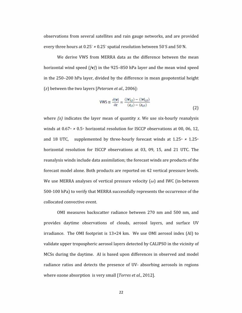
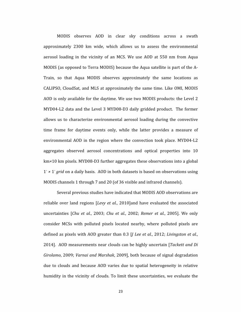
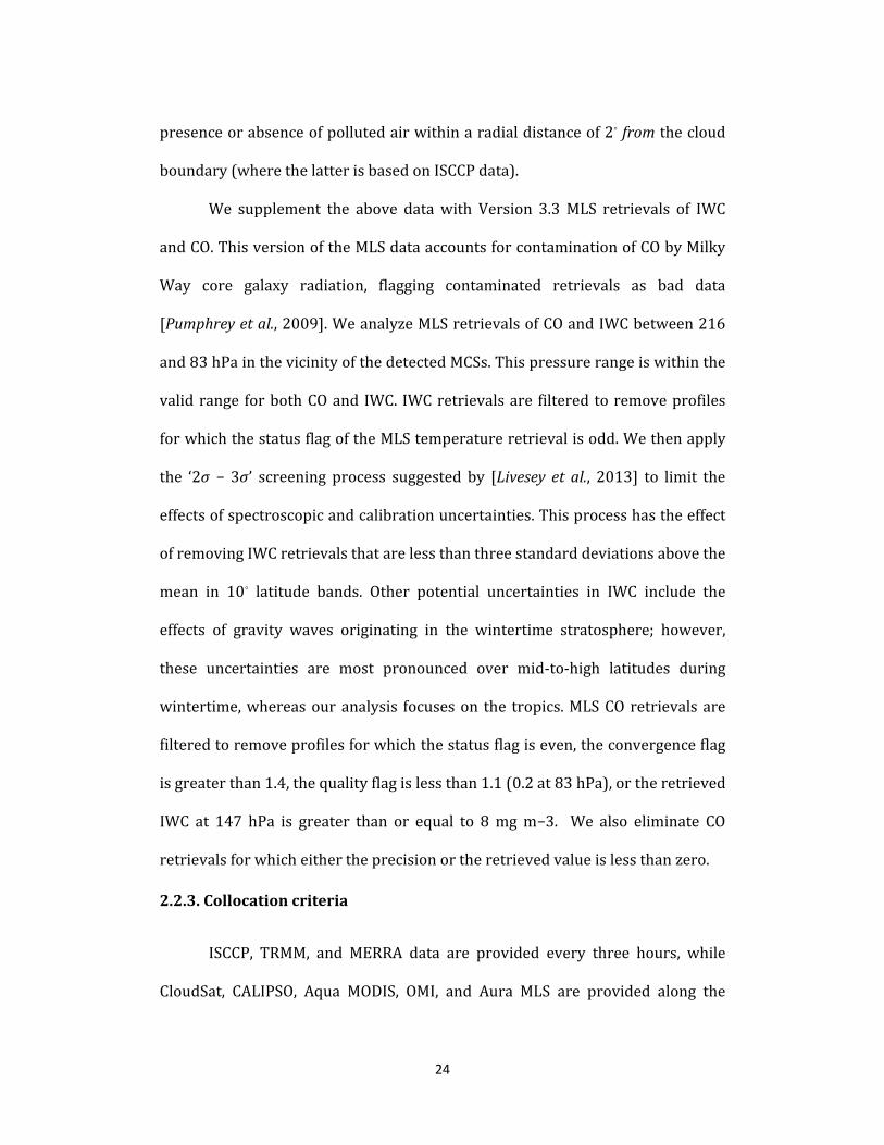
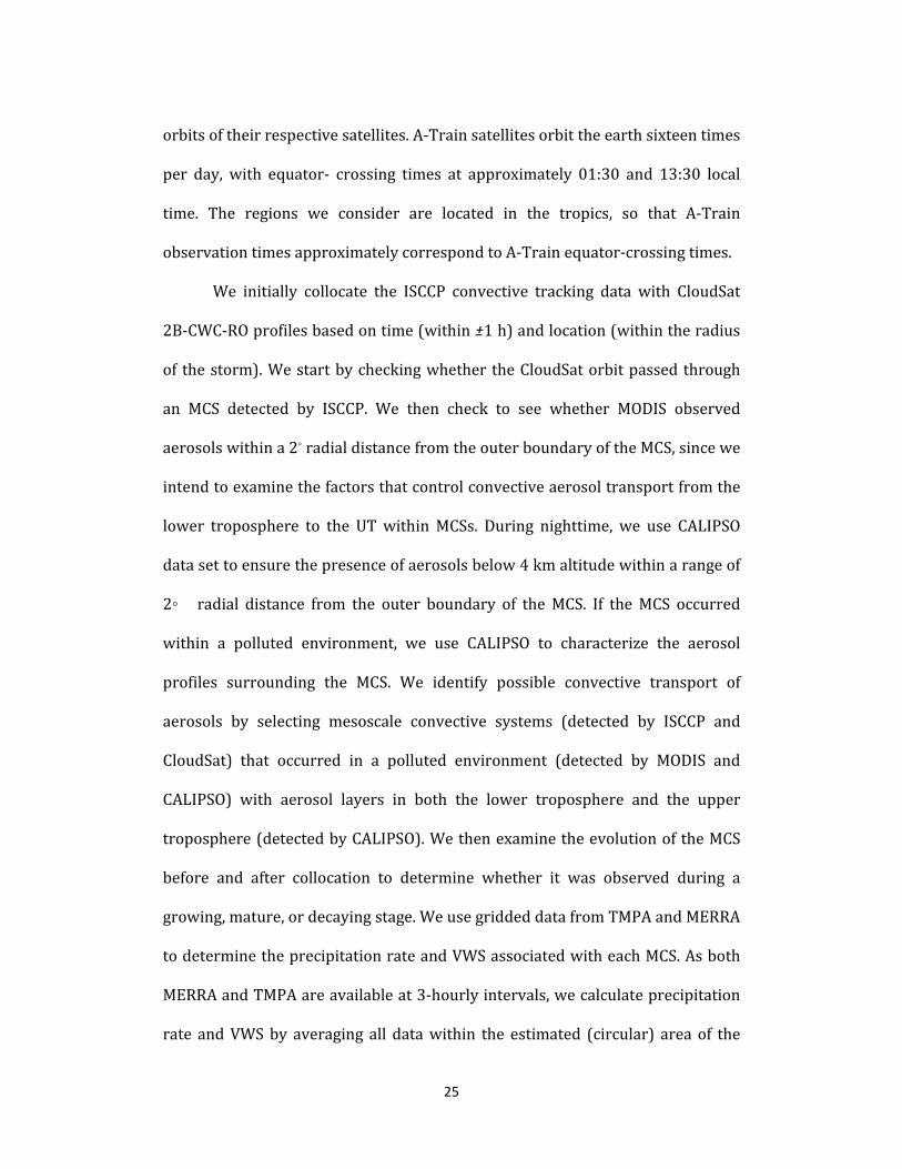
(z)betweenthetwolayers[Petersenetal.,2006]:

(2)

where (x) indicates the layermean of quantity x.We use six‐hourly reanalysis

windsat0.67◦×0.5◦horizontalresolutionforISCCPobservationsat00,06,12,

and 18 UTC, supplemented by three‐hourly forecast winds at 1.25◦ × 1.25◦

horizontal resolution for ISCCP observations at 03, 09, 15, and 21 UTC. The

reanalysiswindsincludedataassimilation;theforecastwindsareproductsofthe

forecastmodelalone.Bothproductsarereportedon42verticalpressurelevels.

WeuseMERRAanalysesofverticalpressurevelocity(ω)and IWC(in‐between

500‐100hPa)toverifythatMERRAsuccessfullyrepresentstheoccurrenceofthe

collocatedconvectiveevent.

OMImeasures backscatter radiance between 270 nm and 500 nm, and

provides daytime observations of clouds, aerosol layers, and surface UV

irradiance. TheOMI footprint is13×24km. WeuseOMIaerosol index (AI) to

validateuppertroposphericaerosollayersdetectedbyCALIPSOinthevicinityof

MCSsduring thedaytime. AI isbasedupondifferences inobservedandmodel

radiance ratios and detects the presence of UV‐ absorbing aerosols in regions

whereozoneabsorptionisverysmall[Torresetal.,2012].

23

MODIS observes AOD in clear sky conditions across a swath

approximately 2300 km wide, which allows us to assess the environmental

aerosol loading in the vicinity of an MCS.We use AOD at 550 nm from Aqua

MODIS(asopposedtoTerraMODIS)becausetheAquasatelliteispartoftheA‐

Train, so that Aqua MODIS observes approximately the same locations as

CALIPSO,CloudSat, andMLSatapproximately thesame time.LikeOMI,MODIS

AODisonlyavailableforthedaytime.WeusetwoMODISproducts:theLevel2

MYD04‐L2dataand theLevel3MYD08‐D3dailygriddedproduct. The former

allows us to characterize environmental aerosol loading during the convective

time frame for daytime events only, while the latter provides a measure of

environmental AOD in the regionwhere the convection took place.MYD04‐L2

aggregates observed aerosol concentrations and optical properties into 10

km×10kmpixels.MYD08‐D3furtheraggregatestheseobservationsintoaglobal

1◦×1◦gridonadailybasis.AODinbothdatasetsisbasedonobservationsusing

MODISchannels1through7and20(of36visibleandinfraredchannels).

SeveralpreviousstudieshaveindicatedthatMODISAODobservationsare

reliable over land regions [Levy etal., 2010]andhave evaluated the associated

uncertainties [Chu et al., 2003; Chu et al., 2002; Remer et al., 2005]. We only

consider MCSs with polluted pixels located nearby, where polluted pixels are

definedaspixelswithAODgreater than0.3 [JLeeetal.,2012;Livingstonetal.,

2014]. AODmeasurementsnearcloudscanbehighlyuncertain[TackettandDi

Girolamo,2009;VarnaiandMarshak,2009],bothbecauseofsignaldegradation

due to clouds and because AOD varies due to spatial heterogeneity in relative

humidity in thevicinityof clouds.To limit theseuncertainties,weevaluate the

24

presenceorabsenceofpollutedairwithinaradialdistanceof2◦fromthecloud

boundary(wherethelatterisbasedonISCCPdata).

We supplement the above datawith Version 3.3MLS retrievals of IWC

andCO.ThisversionoftheMLSdataaccountsforcontaminationofCObyMilky

Way core galaxy radiation, flagging contaminated retrievals as bad data

[Pumphreyetal.,2009].WeanalyzeMLSretrievalsofCOandIWCbetween216

and83hPainthevicinityofthedetectedMCSs.Thispressurerangeiswithinthe

validrange forbothCOandIWC. IWCretrievalsare filteredtoremoveprofiles

forwhichthestatusflagoftheMLStemperatureretrievalisodd.Wethenapply

the ‘2σ −3σ’ screening process suggested by [Livesey etal., 2013] to limit the

effectsofspectroscopicandcalibrationuncertainties.Thisprocesshastheeffect

ofremovingIWCretrievalsthatarelessthanthreestandarddeviationsabovethe

mean in 10◦ latitude bands. Other potential uncertainties in IWC include the

effects of gravity waves originating in the wintertime stratosphere; however,

these uncertainties are most pronounced over mid‐to‐high latitudes during

wintertime,whereasouranalysis focuseson the tropics.MLSCOretrievals are

filteredtoremoveprofilesforwhichthestatusflagiseven,theconvergenceflag

isgreaterthan1.4,thequalityflagislessthan1.1(0.2at83hPa),ortheretrieved

IWC at 147 hPa is greater than or equal to 8mgm−3. We also eliminate CO

retrievalsforwhicheithertheprecisionortheretrievedvalueislessthanzero.

2.2.3.Collocationcriteria

ISCCP, TRMM, and MERRA data are provided every three hours, while

CloudSat, CALIPSO, Aqua MODIS, OMI, and Aura MLS are provided along the

25

orbitsoftheirrespectivesatellites.A‐Trainsatellitesorbittheearthsixteentimes

per day, with equator‐ crossing times at approximately 01:30 and 13:30 local

time. The regions we consider are located in the tropics, so that A‐Train

observationtimesapproximatelycorrespondtoA‐Trainequator‐crossingtimes.

We initially collocate the ISCCP convective tracking data with CloudSat

2B‐CWC‐ROprofilesbasedontime(within±1h)andlocation(withintheradius

of thestorm).Westartbycheckingwhether theCloudSatorbitpassedthrough

an MCS detected by ISCCP. We then check to see whether MODIS observed

aerosolswithina2◦radialdistancefromtheouterboundaryoftheMCS,sincewe

intendtoexaminethefactorsthatcontrolconvectiveaerosoltransportfromthe

lower troposphere to the UTwithinMCSs. During nighttime, we use CALIPSO

datasettoensurethepresenceofaerosolsbelow4kmaltitudewithinarangeof

2◦ radial distance from the outer boundary of theMCS. If theMCS occurred

within a polluted environment, we use CALIPSO to characterize the aerosol

profiles surrounding the MCS. We identify possible convective transport of

aerosols by selecting mesoscale convective systems (detected by ISCCP and

CloudSat) that occurred in a polluted environment (detected by MODIS and

CALIPSO) with aerosol layers in both the lower troposphere and the upper

troposphere(detectedbyCALIPSO).WethenexaminetheevolutionoftheMCS

before and after collocation to determine whether it was observed during a

growing,mature,ordecayingstage.WeusegriddeddatafromTMPAandMERRA

todeterminetheprecipitationrateandVWSassociatedwitheachMCS.Asboth

MERRAandTMPAareavailableat3‐hourlyintervals,wecalculateprecipitation

rate andVWSby averaging all datawithin the estimated (circular) areaof the

26

cloud indicated by ISCCP (defined by the center and the radius).We use Aura

MLS IWC to supplement observations of deep convection andAuraMLS CO to

supplementobservationsofaerosoltransport[Jiangetal.,2008].

Wevalidate theupper tropospheric aerosol layersdetectedbyCALIPSO

usingOMI(seebelow),andthelowertroposphericaerosol layersusingMODIS.

ThisvalidationislimitedtodaytimeMCSs,becauseMODISandOMIareonlyable

toobserveaerosolsduringtheday.Thislimitationrestrictsthetotalnumberof

collocated samples to 963 (353 growing MCSs, 400 mature MCSs, and 210

decayingMCSs).OMIisabletodistinguishbetweenabsorbingandnon‐absorbing

aerosols:positivevaluesofAIindicatethepresenceofabsorbingaerosols(such

asdust or smoke),whilenear‐zeroornegative values indicate thepresenceof

non‐absorbingaerosolsorcloudparticles.AnOMImeasurementwithAIcloseto

1 and a reflectivity greater than about 0.15 likely indicates a cloud–aerosol

mixture,whileameasurementwithAIlargerthan1andreflectivitylargerthan

0.25 likely indicates aerosols above clouds (Dr. Omar Torres, personal

communication, 3 October 2011). 79% of collocated OMI and CALIPSO

measurements inthevicinityofconvectiveanvilsagreeregardingthepresence

(orabsence)ofaerosolsatthecloudtop.

Torres et al. [2012] used simultaneous measurements from A‐Train

satellites (specifically CALIPSO, MODIS, and OMI) to detect the properties of

aerosol and cloud layers over the southern Atlantic Ocean. They used large

valuesofAImeasuredbyOMI to identify thepresenceof aerosol layers above

clouds,andCALIPSOmeasurementsat532nmtodeduceinformationaboutthe

vertical profile of aerosols and clouds. CALIPSO consistently confirmed the

27

presenceofenhancedaerosollayersabovecloudsobservedbyOMI.Theyfurther

usedMODIStruecolorimagestodeterminethehorizontalextentoftheobserved

clouds. The success of their study and others [Yu et al., 2012] shows that

approximately simultaneousmeasurementsmade by satellites (such as the A‐

Trainsatellites,whichfolloweachotheratamaximumintervalof�15minutes)

can be used to describe the collective properties of cloud and aerosol layers.

Moreover, measurements from additional satellite instruments provide

independentsupportandvalidationofthecoredatasetsweuseinthisstudy.

Figure2showsanexampleofA‐Trainsatellitemeasurementscollocated

withanMCSidentifiedandtrackedusingISCCPdata.TheISCCPdataprovidethe

locationof thecenterand theradiusof thesystemevery threehours (Fig.2a).

ThisMCSwas firstobservedover the southernAmazon (16.7◦S,57.3◦W)at21

UTC on 20 January 2007. The MCS moved west as it developed, where it

intersected with the A‐Train tracks at approximately 06 UTC on 21 January

2007,whentheMCSwasinagrowingstage(AE=0.36).Theradiusofthesystem

grewfrom158kmat03UTCto228kmat06UTC.AccordingtocollocatedTMPA

data, themean precipitation rate at this time was 0.69mm h−1. CALIPSO and

CloudSatpassedovertheeasternsideoftheMCSasitmovedwestwardat05:27

UTC, andAuraMLSpassedover justwestof the centerof the systemat05:35

UTC.Theconvectionbegantodecayafter09UTC,eventuallydisappearingafter

15UTCon21January2007.ItwasonlyobservedbytheA‐Trainsatellitesonce.

Figure 2b shows profiles of IWC and increases in CO relative to

background concentrations (calculated as the mean clear‐sky CO observed

within1000kmofthesystemon21January2007)retrievedbyAuraMLSduring

28

theoverpassofthissystem.LargevaluesofIWCwereobservedbothwithinthe

systemandimmediatelytoitsnorth,withamaximumvalueof43mgm−3.Large

positiveCOanomaliesabovethestormindicatethatpollutedairwastransported

totheuppertroposphere,particularlynearthegeographiccenterofthesystem.

Figure2cshowsobservationsofcloudandaerosollayersmadebyCloud‐Satand

CALIPSOastheypassedoverthesystem.TheCALIPSOmeasurementsshowboth

extensive anvil layers and aerosol layers in the upper troposphere,

approximately 10–12 km above the surface on either sides of the MCS in‐

between10◦Sand22◦S.Theverticalcloudlayerat10◦Sisdetectedwithloworno

confidencebytheCADalgorithmandistermedasfalsedetermination.However,

the columnar layerof aerosolsdetectedat9◦S isnot a falsedeterminationand

indicates a real aerosol feature. CloudSat profiled the vertical structure of the

centralpartof the cloudsystem,whichCALIPSOwaspartiallyunable todetect

due toattenuation in the lidarsignal.LargevaluesofCWC(indicativeofNCCs)

wereobservedwithinthesystem,particularlynearitsnorthernedge.

CloudSat and CALIPSO observations collected during overpasses that

passedclosetothecenterofanMCScanbeusedtoverifythesizeandlocationof

thesameMCSreportedbyISCCP.CloudsizesbasedonCALIPSOobservationsof

anvilcloudsareslightlygreaterthanthosereportedbyISCCP,whilecloudsizes

basedonCloudSatobservationsare slightly less than those reportedby ISCCP.

These differences can be explained by differences in the sensitivities of these

instrumentstosmalliceparticlesandopticallythinclouds.Thecentrallocation

of MCSs based on CloudSat is within ±1◦ of the center reported by ISCCP.

Differences in the central location could be attributable to horizontal

29

propagation of the stormduring the time gapbetweenwhen it is observedby

ISCCPandwhenitisobservedbytheA‐Trainsatellites.

Theoccurrenceofconvectiveaerosol transport is inferred fromchanges

in the vertical distribution of aerosol pixels relative to expected background

values.Thebackgroundprofileofaerosolpixelsisderivedbyaveragingallclear‐

skyCALIPSOdataoveronemonthina1◦×1◦gridboxwithaverticalresolution

of 1 km between the surface and 20 km altitude. Aerosol pixel counts near

convectionaredefinedas thenumberofaerosolpixelsalongthesatellite track

within±2◦(222km)oftheboundaryoftheMCSalongthesatellitetrack,butnot

withinthesystemitself.Aerosolpixelcountsarethuscalculatedalongthesame

horizontal length on both sides of every system, regardless of its size. The

backgroundprofilefromthegridcellcontainingtheMCSissubtractedfromthe

number of aerosol pixels observed in the vicinity of the convection at each

altitude. The differences are then binned in 2 km vertical increments. For

example,thechangeinthenumberofaerosolpixelsat9kmaltitudeisdefinedas

thesumofdifferencesbetweentheobservedandbackgroundprofilesinthe8–9

kmand9–10kmlayers.Thisproceduremitigatesuncertaintiesassociatedwith

horizontal advection of aerosols into the vicinity of the MCS. The vertical

distributionsof convectivedetrainmentheightbasedonCloudSat IWC(Fig. 3)

andMERRAverticalvelocity (notshown)alsosupport the hypothesis that the

detected aerosol layers are primarily transported to the UT by the collocated

convectivesystems.Thenumberofbackgroundaerosolpixelsisverylowabove

4kmaltitude,consistentwithpreviousresultsbasedonCALIPSO[Huangetal.,

2013] and Department of Energy Atmospheric Radiation Measurement (ARM)

30

observations [Turner et al., 2001]. The detected aerosols are unlikely to be

freshly nucleated, as previous studies indicate that only a small number of

nucleationmodeaerosolsreachtheconvectiveanvil[Ekmanetal.,2006].Hence,

we use the vertically integrated extent of the convective aerosol layers (ALs),

defined as the total number of aerosol pixels between 4 and 20 kmwithin a

rangeof2◦ radialdistance fromtheouterboundaryof theMCS, toexplorethe

influenceofconvectivedynamicpropertiesonaerosoltransport.

Due to laser attenuation, CALIPSO can only observe aerosols near the

periphery of the cloud systems; it cannot detect aerosols inside clouds with

substantialwatercontent(see,e.g.,Fig. 2c).Ouranalysis is thereforebasedon

aerosolprofilesdetectedontheperipheryofMCSs,eitheraboveorbeneaththe

stratiformportionsofthesystem.AquaMODISandOMIarecompletelyunableto

detectaerosollayersunderneathclouds.Theseinstrumentsarenotsuitablefor

detectingaerosolswhentheCWCislarge.

We useMERRA data to provide ameteorological context for eachMCS,

includingthegrid‐scaleverticalpressurevelocity(ω)andtheverticalwindshear

(VWS) intheareasurroundingtheconvection.Theoccurrenceofconvectionin

MERRAmatcheswellwiththeoccurrenceofconvectionobservedbytheA‐Train

satellites.MERRA simulates strong negative values ofω (indicative of upward

motion) and detects IWC in‐between 500‐100 hPa (indicative of presence of a

system extending from mid altitudes to anvil level) in 98% of the collocated

cases.Weeliminatetheother2%ofcasesfromtheanalysis.

Ourstudyincludesatotalof963MCSs(systemswithlifetimesmorethan

6hours)overequatorialAfrica,SouthAsia,andtheAmazonbasinbetweenJune

31

2006andJune2008.WerestrictouranalysisofMCSsoverSouthAsiatosystems

thatoccurredduringthepeakmonsoonmonths(June–August2006,June–August

2007, and June 2008). The 963 identified systems include 353 growingMCSs,

400matureMCSs,and210decayingMCSs.Wealsobrieflyexamine111short‐

lived convective systems (systems with lifetimes less than 6 hours) over the

Amazonbasin.

Our collocation methodology (Section 2.3) contains several potential

sourcesofrandomerror,suchasmeasurementuncertaintiesanddifferencesin

the part of the MCS observed by the A‐Train satellite instruments (e.g., edge

versus center, convective versus stratiformparts of theMCS, etc.). Tomitigate

the effects of these random errors, we aggregate each sample into 50 bins of

approximately equal size according to the observed aerosol layer extent and

performtheregressionusingthemeanvaluesineachbin.Forexample,thefull

sampleof963MCSs isseparated into50bins,eachcontainingbetween19and

20MCSs.Missingdataaremaskedandexcludedfromthemeanvalueineachbin.

2.2.4.Statisticalmodelconstruction

The statistical models we consider here are based on multiple linear

regression, inwhich thedependent variable (oroutput) ismodeledas a linear

combinationoftheindependentvariables(orpredictors):

whereβ0istheinterceptandβj,j∈[1,p]isthecoefficientassociatedwiththejth

of p predictors. In our analysis, the dependent variable yi is the aerosol layer

32

extent,definedastheaerosolpixelcountrelativetothelocalbackgroundaerosol

pixelcountbasedonCALIPSOobservations.Thisvariablecanbeeithernegative

(indicating dilution of the upper tropospheric background aerosol layer) or

positive(indicatingaerosoltransport).Theindependentvariablesxijincludethe

radius,numberofconvectivecores(NCC),andconvectivefraction(CF)observed

from ISCCP data, the cloud top height (CTH) from CALIPSO, the vertical wind

shear (VWS) fromMERRA, the precipitation rate fromTRMM, and the aerosol

opticaldepth(AOD)fromMODIS(i.e.,p=7).Westandardizeallpredictorssothat

theyhaveameanofzeroandavarianceofone.

Traditional linearregressionselectsthecoefficientsβˆ thatminimizethe

residualsumofsumofsquares;

This approach is unsuited to coefficient determination and variable

selection formodelingphysical systems likedeepconvection, forwhich twoor

moreofthepredictorsmaybetightlycorrelated.Inparticular,thecoefficientsfor

tightly correlated predictors may be large, with opposite signs that cause

compensation in the model. To mitigate this effect, we apply the elastic net

method forcoefficientshrinkage [ZouandHastie, 2005].Thismethodappliesa

penaltyonthesizeofthecoefficients.Thecoefficientsβˆarethendeterminedby

minimizingthepenalizedresidualsumofsquares

33

Ourgoalistoidentifythesubsetofpredictorsthatbestexplainvariability

in the dependent variable. We therefore use recursive feature elimination to

identifysubsetsof independentvariables thatmaximize theexplainedvariance

in the sample. It eliminates the redundant or irrelevant independent variables

thatmakeno useful contribution inpredicting the dependent variable.We are

thenleftwithsevensubsetswithsizesofonetoseven,wherethesubsetofsize

one includes the single predictor that maximizes the explained variance, the

subsetof size two includes thepairofpredictors thatmaximizes theexplained

variance,andsoon.Thesubsetofsizesevenincludesallsevenpredictors.

Weapplyarandomfive‐foldcross‐validationtotrainandtestthemodels

usingoptimalsubsetsofvarioussize.Specifically,werandomlydividethesample

into fiveapproximatelyequalbins.Wethenuse80%of thedata toconstructa

statisticalmodelbasedoneachoptimalsubsetofsizeonetoseven,andthentest

the model using the remaining 20% of the data. This approach is applied

recursively, so thateach20% isusedas testdata.Werepeat this random five‐

fold cross‐validation process 100 times, so that 500 models are trained and

tested. We then calculate the coefficients βˆ as the average coef icients over

those 500 models. Repeating this process generally results in identical

coefficientstothreesignificantdigits.

∑ | |isoftenreferredtoastheL1prior(usedinLassoregression)and

thepenalty∑ | 2 |isreferredtoasL2prior(usedinridgeregression).

34

Figure 2. An example of a collocated MCS, including (a) the origin anddevelopment of theMCS, (b) thevertical distributionof IWCand fractionalCOanomalies in the upper troposphere along the MLS track, and (c) the verticaldistributionof aerosol andcloud layersalong theCALIPSOandCloudSat track.ThisMCSwasfirstdetectedbyISCCPat21UTC20January2007at16.7∘Sand57.3∘W.Thesystemthenmovedwest,wheretheA‐Trainsatellitesobserveditatapproximately06UTC21 January.Thedarkand lightblue circles inFigure2ashow the approximate central position and radius of the MCS at the A‐Trainoverpass time. The cloudwas growingwhen CALIPSO and CloudSat (red line)observeditstrailingedgeat05:27UTCandAuraMLS(greenline)observedthesystem near its center at 05:35 UTC. The central positions of each satellitefootprintareshownaswhitecirclesalongthesatellitetrack.

35

Theoptimalmodel ischosenbyidentifyingthesubsetofindependentvariables

thatminimizesthemeansquarederrorinthetestdata.Choosingamodelthatis

toosimple(i.e.,includingtoofewpredictors)willunderfitthetrainingdata,with

errors in the testdatadominatedby largebiases.Choosingamodel that is too

complex(i.e., includingtoomanypredictors)willoverfit thetrainingdata,with

errorsinthetestdatadominatedbylargevariance.Usingthisprocedure,weare

able to construct statistical learning models that strike a balance between

maximizing explained variance (via recursive feature elimination) and

minimizingmeansquarederror(viacross‐validation).

2.3Results

Inprinciple, aerosols canbe transported to theUTbyeither long‐range

transport or by local convective transport. The slopes of isentropic surfaces,

sedimentation, andverticalmotiondrivenbydiabatic heating canall influence

theheightofanaerosollayer,sothattheverticaldistributionofaerosollayersis

unlikely to remain constant during long‐range transport. By contrast, the

vertical locations of aerosol layers recently transported to the UT by local

convective transportare likely tomatch thevertical locationsof theassociated

convectivedetrainmentlayers.Figure3showsthedistributionsofaerosollayer

height(HAL),clouddetrainmentheight(HDL),andcloudtopheight(CTH)forall

MCSs detected by ISCCP with aerosol layers in the upper troposphere. The

vertical distribution of aerosol layers observed in the vicinity of convection is

verysimilar to theverticaldistributionofconvectivedetrainmentheights.This

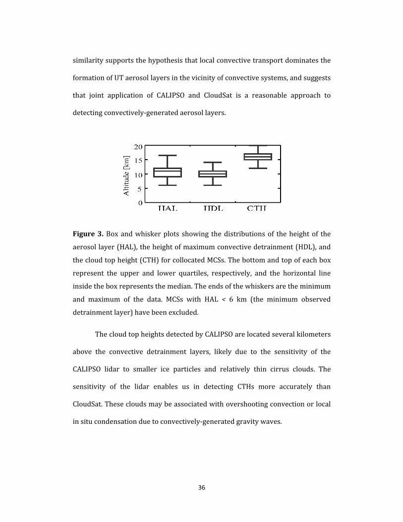
36

similaritysupportsthehypothesisthatlocalconvectivetransportdominatesthe

formationofUTaerosollayersinthevicinityofconvectivesystems,andsuggests

that joint application of CALIPSO and CloudSat is a reasonable approach to

detectingconvectively‐generatedaerosollayers.

Figure3.Boxandwhiskerplots showing thedistributionsof theheightof the

aerosollayer(HAL),theheightofmaximumconvectivedetrainment(HDL),and

thecloudtopheight(CTH)forcollocatedMCSs.Thebottomandtopofeachbox

represent the upper and lower quartiles, respectively, and the horizontal line

insidetheboxrepresentsthemedian.Theendsofthewhiskersaretheminimum

and maximum of the data. MCSs with HAL < 6 km (the minimum observed

detrainmentlayer)havebeenexcluded.

ThecloudtopheightsdetectedbyCALIPSOarelocatedseveralkilometers

above the convective detrainment layers, likely due to the sensitivity of the

CALIPSO lidar to smaller ice particles and relatively thin cirrus clouds. The

sensitivity of the lidar enables us in detecting CTHs more accurately than

CloudSat.Thesecloudsmaybeassociatedwithovershootingconvectionorlocal

insitucondensationduetoconvectively‐generatedgravitywaves.

37

Figure4.Meanprofilesof(a)IWCand(b)COintheuppertropospherebasedon

AuraMLSprofilescollocatedwithgrowing(red),mature(purple),anddecaying

(blue) MCSs. Shading represents intervals of one standard error around the

mean.

Figure4showsvariationsinIWCandCOintheuppertroposphereduring

differentstagesofconvectivedevelopment.Both IWCandCO tend tobe larger

duringthegrowingstagethanduringthematureordecayingstages.Thisresult

indicates that convection is typically deepest and most intense during the

growingstage,withstrongertransportofnear‐surfaceairtotheUT.

ThishypothesisisfurthersupportedbyFig.5,whichshowsvariationsin

aerosol transport and convective properties during different stages of the

convective life cycle. The vertically‐integrated extent of the convective aerosol

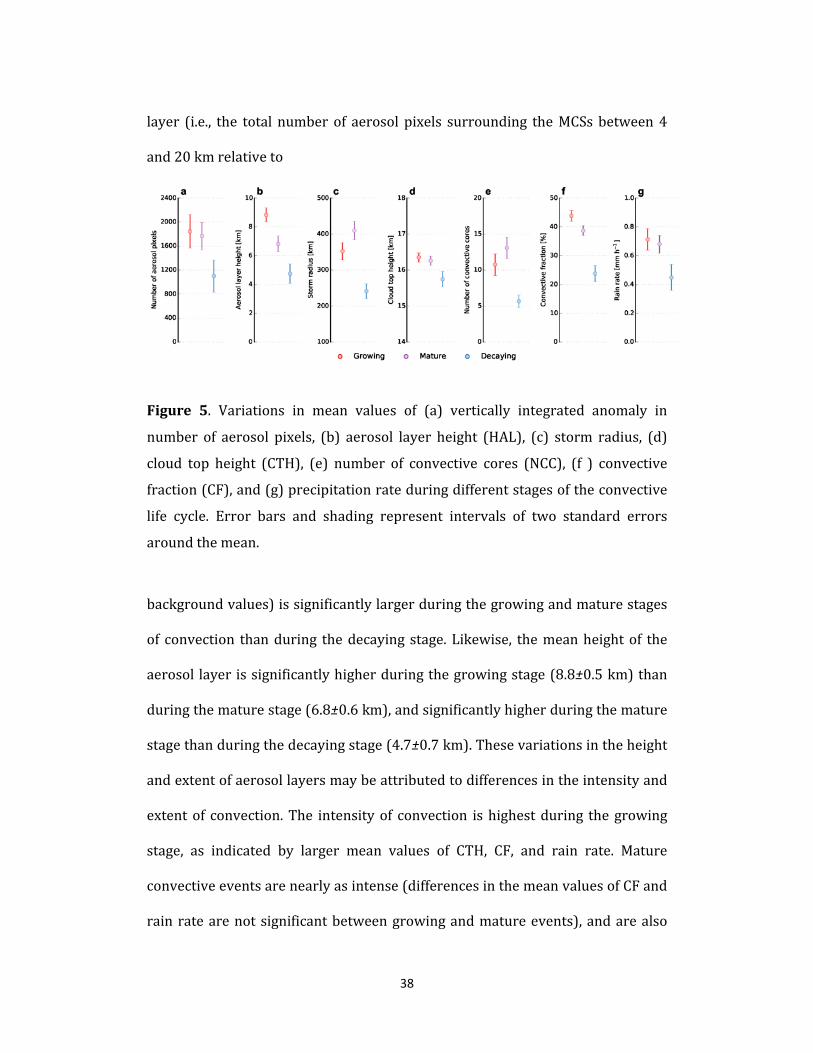
38

layer (i.e., the total number of aerosol pixels surrounding theMCSsbetween4

and20kmrelativeto

Figure 5. Variations in mean values of (a) vertically integrated anomaly in

number of aerosol pixels, (b) aerosol layer height (HAL), (c) storm radius, (d)

cloud top height (CTH), (e) number of convective cores (NCC), (f ) convective

fraction(CF),and(g)precipitationrateduringdifferentstagesoftheconvective

life cycle. Error bars and shading represent intervals of two standard errors

aroundthemean.

backgroundvalues)issignificantlylargerduringthegrowingandmaturestages

of convection thanduring thedecaying stage.Likewise, themeanheightof the

aerosol layerissignificantlyhigherduringthegrowingstage(8.8±0.5km)than

duringthematurestage(6.8±0.6km),andsignificantlyhigherduringthemature

stagethanduringthedecayingstage(4.7±0.7km).Thesevariationsintheheight

andextentofaerosollayersmaybeattributedtodifferencesintheintensityand

extentof convection.The intensityof convection ishighestduring thegrowing

stage, as indicated by larger mean values of CTH, CF, and rain rate. Mature

convectiveeventsarenearlyasintense(differencesinthemeanvaluesofCFand

rainratearenotsignificantbetweengrowingandmatureevents),andarealso

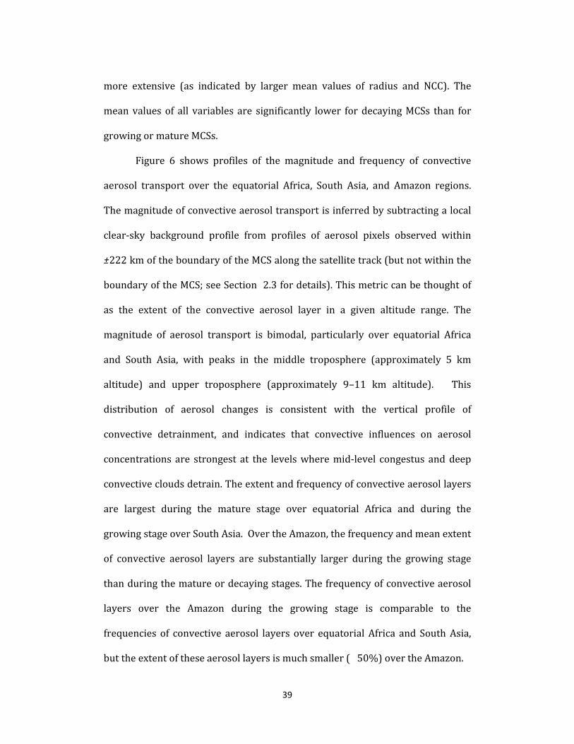
39

more extensive (as indicated by larger mean values of radius and NCC). The

meanvaluesof all variables are significantly lower fordecayingMCSs than for

growingormatureMCSs.

Figure 6 shows profiles of the magnitude and frequency of convective

aerosol transport over the equatorial Africa, South Asia, and Amazon regions.

Themagnitudeofconvectiveaerosoltransportisinferredbysubtractingalocal

clear‐sky background profile from profiles of aerosol pixels observed within

±222kmoftheboundaryoftheMCSalongthesatellitetrack(butnotwithinthe

boundaryoftheMCS;seeSection2.3fordetails).Thismetriccanbethoughtof

as the extent of the convective aerosol layer in a given altitude range. The

magnitude of aerosol transport is bimodal, particularly over equatorial Africa

and South Asia, with peaks in the middle troposphere (approximately 5 km

altitude) and upper troposphere (approximately 9–11 km altitude). This

distribution of aerosol changes is consistent with the vertical profile of

convective detrainment, and indicates that convective influences on aerosol

concentrations are strongest at the levelswheremid‐level congestus anddeep

convectivecloudsdetrain.Theextentandfrequencyofconvectiveaerosollayers

are largest during the mature stage over equatorial Africa and during the

growingstageoverSouthAsia.OvertheAmazon,thefrequencyandmeanextent

of convective aerosol layers are substantially larger during the growing stage

thanduringthematureordecayingstages.Thefrequencyofconvectiveaerosol

layers over the Amazon during the growing stage is comparable to the

frequencies of convective aerosol layers over equatorialAfrica and SouthAsia,

buttheextentoftheseaerosollayersismuchsmaller(�50%)overtheAmazon.

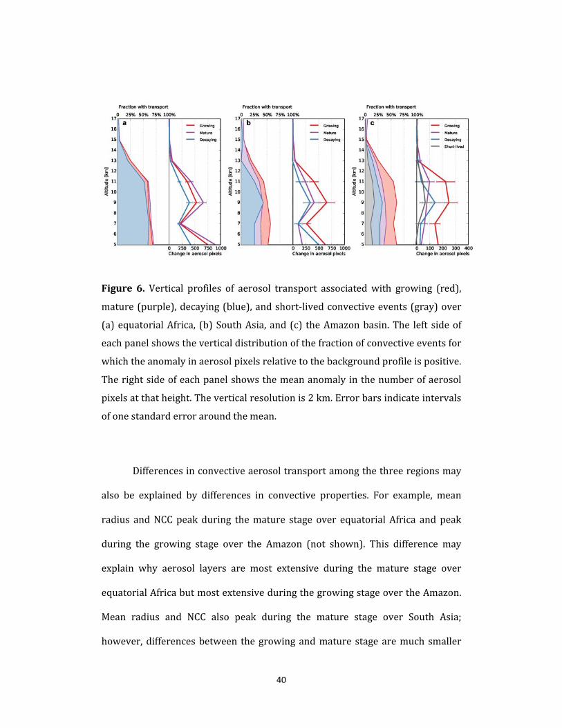
40

Figure6.Vertical profiles of aerosol transport associatedwith growing (red),

mature(purple),decaying(blue),andshort‐livedconvectiveevents(gray)over

(a)equatorialAfrica, (b)SouthAsia, and (c) theAmazonbasin.The left sideof

eachpanelshowstheverticaldistributionofthefractionofconvectiveeventsfor

whichtheanomalyinaerosolpixelsrelativetothebackgroundprofileispositive.

Therightsideofeachpanelshowsthemeananomalyinthenumberofaerosol

pixelsatthatheight.Theverticalresolutionis2km.Errorbarsindicateintervals

ofonestandarderroraroundthemean.

Differencesinconvectiveaerosoltransportamongthethreeregionsmay

also be explained by differences in convective properties. For example, mean

radius andNCCpeakduring themature stage over equatorial Africa and peak

during the growing stage over the Amazon (not shown). This difference may

explain why aerosol layers are most extensive during the mature stage over

equatorialAfricabutmostextensiveduringthegrowingstageovertheAmazon.

Mean radius and NCC also peak during the mature stage over South Asia;

however, differencesbetween thegrowingandmature stagearemuch smaller

41

over South Asia than over equatorial Africa. Moreover, unlike over equatorial

Africa, these differences are not statistically significant. Growing systems are

almostas largeasmaturesystemsoverSouthAsia(meanradiusof438.2±55.6

km relative to 499.3±57.7 km) and have nearly as many convective cores

(18.6±4.8 relative to 20.5±4.6). When coupled with the greater intensity of

growingMCSsrelativetomatureMCSsandthegreaterpotentialformatureMCSs

to occur in environmentswith aerosol concentrations already diluted bywet

scavenging,thesedifferencesprovideaplausibleexplanationforwhyconvective

aerosoltransportisstrongestduringthegrowingstageoverSouthAsia.

The smallermean extent of convective aerosol layers over the Amazon

relative to convective aerosol layers over equatorialAfrica and SouthAsia has

several possible explanations. MCSs over the Amazon have a shorter mean

lifetime(~19h),amuchsmallermeanradius(~120km),andhighermeanrain

rates (~1.5 mm h−1) than MCSs over equatorial Africa or South Asia. The

differencesinlifetimeandradiusarelikelytoreducetheareainfluencedbythe

MCSsovertheAmazonrelativetothelarger,longer‐livedsystemsovertheother

regions,while the difference in rain ratemay enhancewet scavenging. Short‐

livedconvectivesystemsarealsomorecommonovertheAmazonthanoverthe

otherregions;thefrequentprecipitationassociatedwiththesesystemsmayact

moreeffectivelytoflushaerosolsoutoftheatmosphere.

Ourresultsindicatethatconvectiveaerosoltransportisstronger,deeper,

andmore frequentduringthegrowingandmaturestagesof theconvective life

cycle thanduring the decaying stage over all three analyzed regions. Although

this conclusion is unsurprising given thewell‐known differences in convective

42

intensitybetweengrowingsystemsanddecayingsystems[Machadoetal.,1998],

itprovidesastrongindicationthatourapproachisabletocapturevariationsin

bothconvectivestructureandaerosoltransport.Wethereforeusethesedatato

construct a series of statistical models. This approach allows us to establish

firmer connections between measures of convective intensity and aerosol

transport, identify themost influential variables, andevaluate thepotential for

using these variables to predict the occurrence and extent of aerosol layers

generatedbyconvectivetransportinMCSs.

2.4.Statisticalmodelresultsanddiscussion

Figure7showsthefractionofvarianceofaerosol layerextentinthefull

datasetexplainedbythepredictorsintheoptimalstatisticalmodelsforMCSsin

differentstagesoftheconvective lifecycle(seeSection2.4 fordetails).Table2

liststheassociatedcoefficientsandevaluationmetricsforeachmodelbasedon

test data alone.Approximately 80%of the variance inUT aerosol layers (ALs)

associatedwithallMCSscanbeexplainedbythreepredictors:radius,NCC,and

VWS. Likewise, approximately 58% of the variance in ALs associated with

growing MCSs can be explained by two predictors (radius and VWS),

approximately75%ofthevariance inALsassociatedwithmatureMCSscanbe

explainedby threepredictors (radius,NCC,andCF)andapproximately52%of

the variance in ALs associated with decaying MCSs can be explained by two

predictors (radiusandAOD).Themost influentialpredictor ineachcase is the

size(radius)oftheMCS.

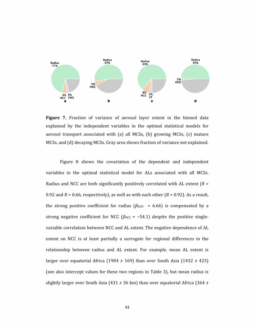
43

Figure 7. Fraction of variance of aerosol layer extent in the binned data

explained by the independent variables in the optimal statistical models for

aerosol transport associated with (a) all MCSs, (b) growing MCSs, (c) mature

MCSs,and(d)decayingMCSs.Grayareashowsfractionofvariancenotexplained.

Figure 8 shows the covariation of the dependent and independent

variables in the optimal statistical model for ALs associated with all MCSs.

RadiusandNCCarebothsignificantlypositivelycorrelatedwithALextent(R=

0.92andR=0.66,respectively),aswellaswitheachother(R=0.92).Asaresult,

the strong positive coefficient for radius (βRAD = 6.66) is compensated by a

strong negative coefficient for NCC (βNCC = −54.1) despite the positive single‐

variablecorrelationbetweenNCCandALextent.ThenegativedependenceofAL

extent on NCC is at least partially a surrogate for regional differences in the

relationship between radius and AL extent. For example, mean AL extent is

larger over equatorial Africa (1904±169) than over SouthAsia (1432±423)

(seealso interceptvalues for these tworegions inTable3),butmeanradius is

slightlylargeroverSouthAsia(431±36km)thanoverequatorialAfrica(364±

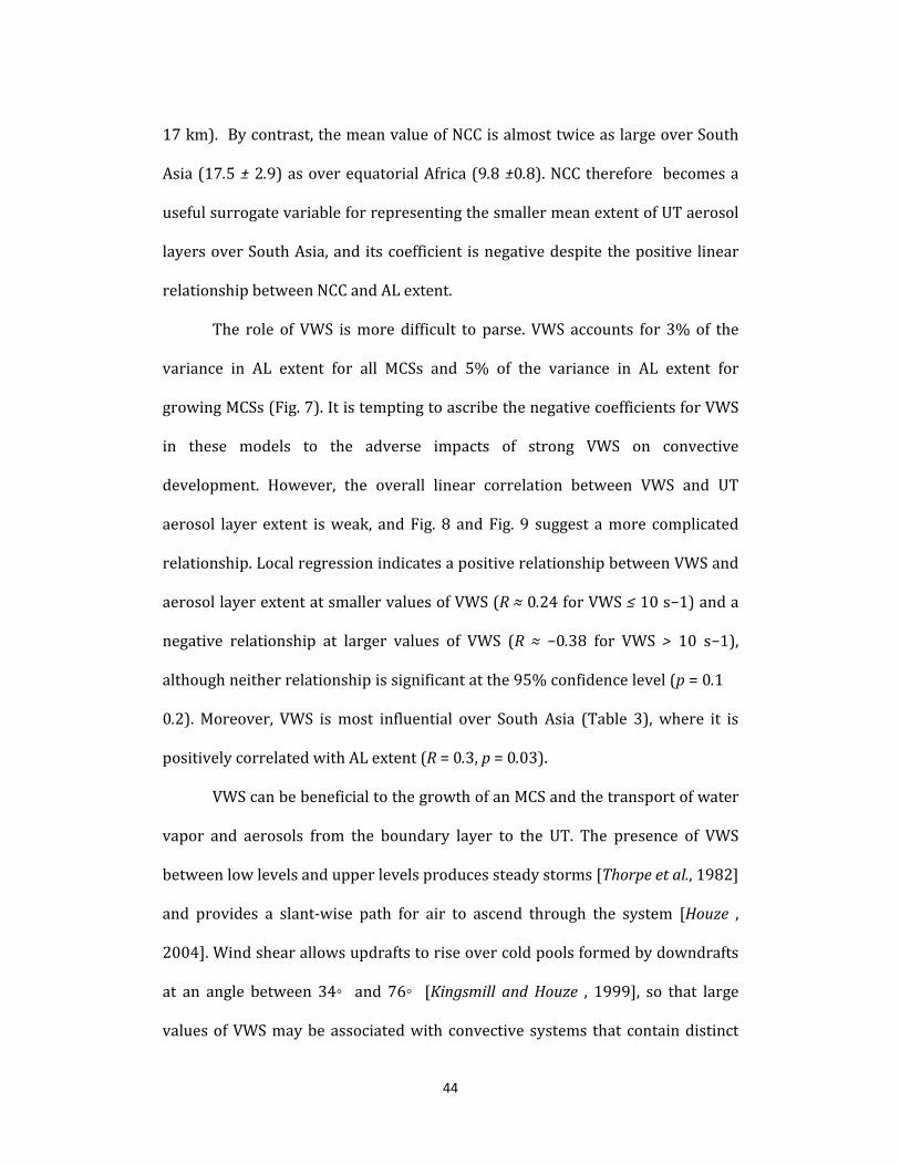
44

17km).Bycontrast,themeanvalueofNCCisalmosttwiceaslargeoverSouth

Asia(17.5±2.9)asoverequatorialAfrica(9.8±0.8).NCCtherefore becomesa

usefulsurrogatevariableforrepresentingthesmallermeanextentofUTaerosol

layersoverSouthAsia,anditscoefficient isnegativedespitethepositive linear

relationshipbetweenNCCandALextent.

The role of VWS ismore difficult to parse. VWS accounts for 3%of the

variance in AL extent for all MCSs and 5% of the variance in AL extent for

growingMCSs(Fig.7).ItistemptingtoascribethenegativecoefficientsforVWS

in these models to the adverse impacts of strong VWS on convective

development. However, the overall linear correlation between VWS and UT

aerosol layer extent isweak, andFig. 8 and Fig. 9 suggest amore complicated

relationship.LocalregressionindicatesapositiverelationshipbetweenVWSand

aerosollayerextentatsmallervaluesofVWS(R≈0.24forVWS≤10s−1)anda

negative relationship at larger values of VWS (R ≈ −0.38 for VWS > 10 s−1),

althoughneitherrelationshipissignificantatthe95%confidencelevel(p=0.1�

0.2).Moreover, VWS ismost influential over South Asia (Table 3), where it is

positivelycorrelatedwithALextent(R=0.3,p=0.03).

VWScanbebeneficialtothegrowthofanMCSandthetransportofwater

vapor and aerosols from the boundary layer to the UT. The presence of VWS

betweenlowlevelsandupperlevelsproducessteadystorms[Thorpeetal.,1982]

and provides a slant‐wise path for air to ascend through the system [Houze ,

2004].Windshearallowsupdraftstoriseovercoldpoolsformedbydowndrafts

at an angle between 34◦ and 76◦ [KingsmillandHouze , 1999], so that large

valuesofVWSmaybeassociatedwithconvectivesystems that containdistinct

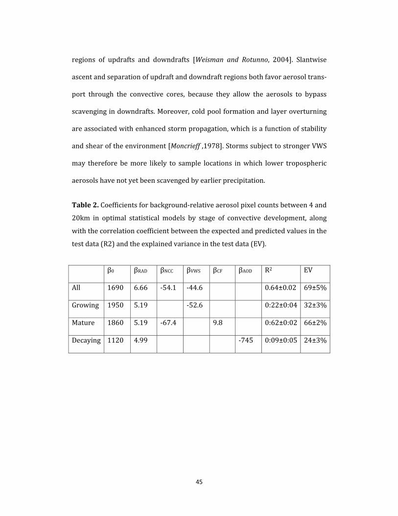
45

regions of updrafts and downdrafts [Weisman and Rotunno, 2004]. Slantwise

ascentandseparationofupdraftanddowndraftregionsbothfavoraerosoltrans‐

port through the convective cores, because they allow the aerosols to bypass

scavengingindowndrafts.Moreover,coldpoolformationandlayeroverturning

areassociatedwithenhancedstormpropagation,whichisafunctionofstability

andshearoftheenvironment[Moncrieff,1978].StormssubjecttostrongerVWS

may therefore bemore likely to sample locations inwhich lower tropospheric

aerosolshavenotyetbeenscavengedbyearlierprecipitation.


20km in optimal statistical models by stage of convective development, along

withthecorrelationcoefficientbetweentheexpectedandpredictedvaluesinthe

testdata(R2)andtheexplainedvarianceinthetestdata(EV).

β0 βRAD βNCC βVWS βCF βAOD R2 EV

All 1690 6.66 ‐54.1 ‐44.6 0.64±0.02 69±5%

Growing 1950 5.19 ‐52.6 0:22±0:04 32±3%

Mature 1860 5.19 ‐67.4 9.8 0:62±0:02 66±2%

Decaying 1120 4.99 ‐745 0:09±0:05 24±3%

46


20kminoptimalstatisticalmodelsbyregiona.

β0 βRAD βNCC βVWS βCF βAOD R2 EV

Africa 1960 5.01

Africa

(G)

2100 4.35

Africa

(M)

2350 5.39 ‐66.1 6.62

Africa

(D)

1300 3.96 ‐776

South

Asia

1632 3.65 57.5

Amazon 475 2.63 ‐98.2

aDataforequatorialAfricaisseparatedintodifferentstagesoftheconvectivelifecycle(G:growing;M:mature;D:decaying).SamplesizesforSouthAsiaandtheAmazonbasinaretoosmalltoseparatebystageofconvectivelifecycle.

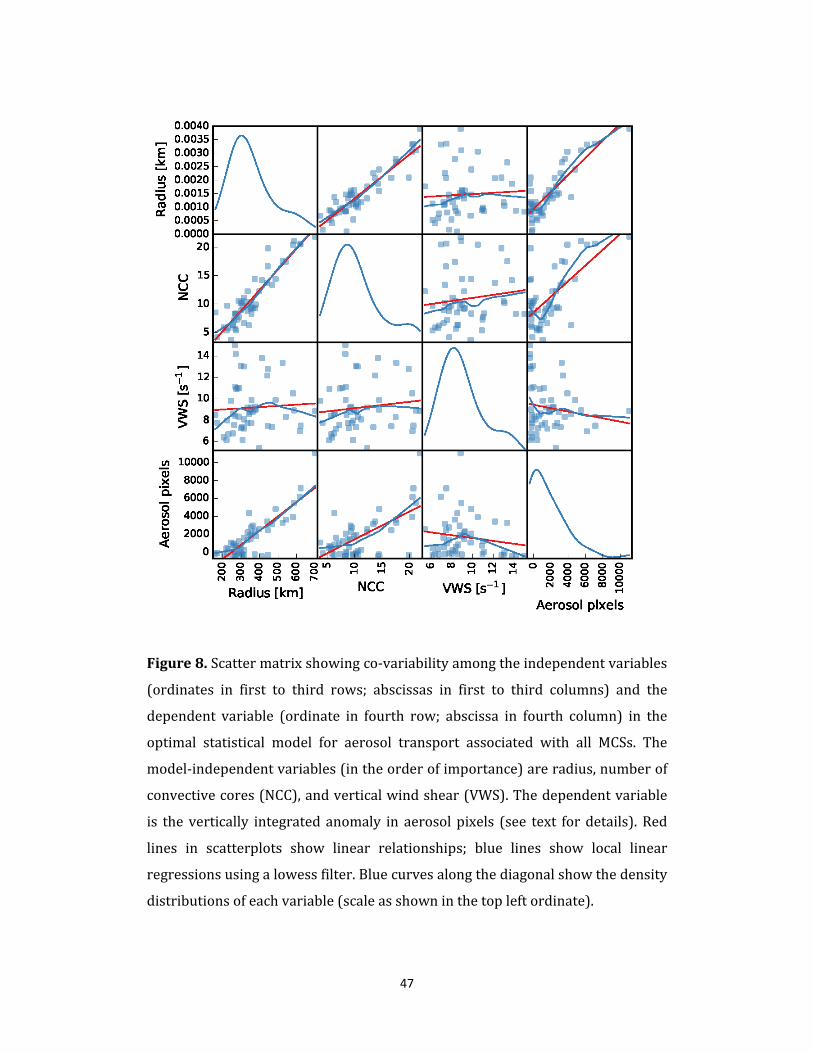
47

Figure8.Scattermatrixshowingco‐variabilityamongtheindependentvariables

(ordinates in first to third rows; abscissas in first to third columns) and the

dependent variable (ordinate in fourth row; abscissa in fourth column) in the

optimal statistical model for aerosol transport associated with all MCSs. The

model‐independentvariables(intheorderofimportance)areradius,numberof

convectivecores(NCC),andverticalwindshear(VWS).Thedependentvariable

is the vertically integratedanomaly in aerosol pixels (see text fordetails).Red

lines in scatterplots show linear relationships; blue lines show local linear

regressionsusingalowessfilter.Bluecurvesalongthediagonalshowthedensity

distributionsofeachvariable(scaleasshowninthetopleftordinate).

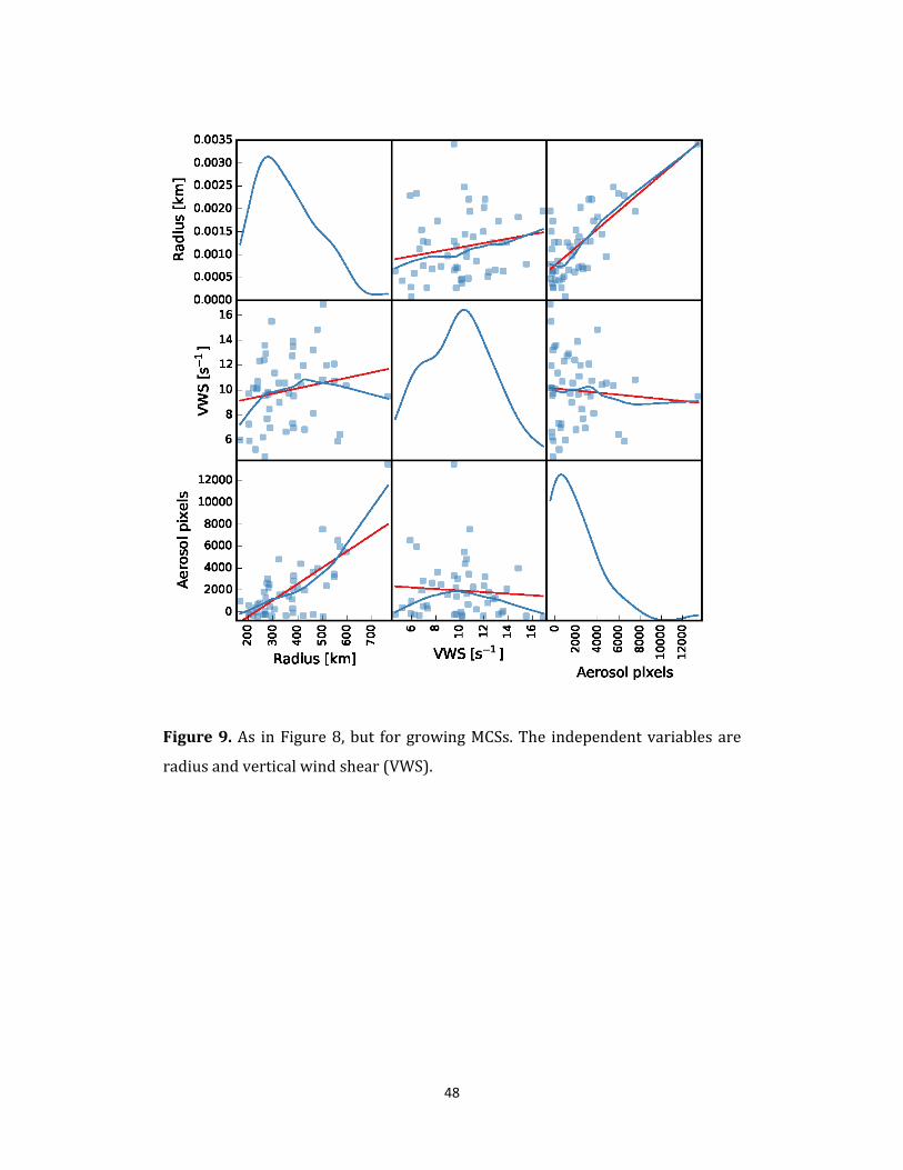
48

Figure9.As inFigure8,but forgrowingMCSs.The independentvariablesare

radiusandverticalwindshear(VWS).

49

Figure10.As inFigure8,but formatureMCSs.The independentvariablesare

radius,numberofconvectivecores(NCC),andconvectivefraction(CF).

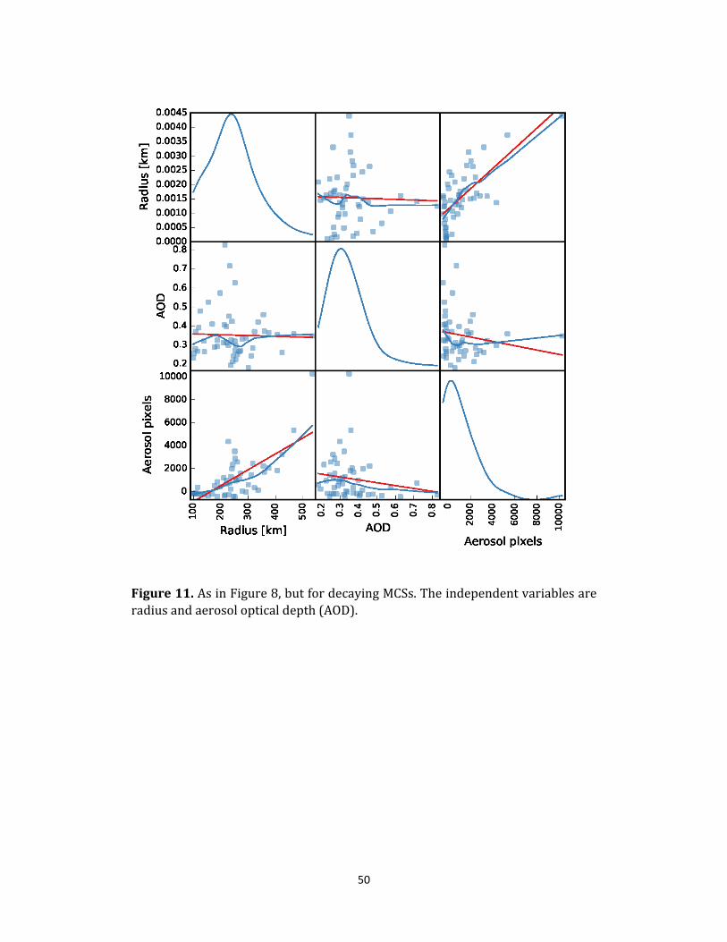
50

Figure11.AsinFigure8,butfordecayingMCSs.Theindependentvariablesareradiusandaerosolopticaldepth(AOD).

51

WeareunabletofullyclarifytherelationshipbetweenVWSandALextent

basedonthesedataalone,butourresultsdopermitsomeinsightthatcouldbe

used todevelopmodel‐based studies to furtherexplore this relationship. First,

the relationship between VWS and AL extent is strongest during the growing

stage. This result is consistent with expectations: growing MCSs are strongly

rooted in the boundary layer,whilematureMCSs aremaintained primarily by

latentheatingandgravitywavedynamicsinthefreetroposphere[Houze,2004]

and decayingMCSs haveweaker updraft speeds and fewer convective cores.

Second, therelationshipbetweenVWSandUTaerosol layerextent is strongest

overSouthAsia. MeanVWSinconvectiveenvironmentsisapproximatelytwice

aslargeoverSouthAsia(15.4±1.1×10−4S−1)asoverequatorialAfrica(7.5±0.5

× 10−4S−1) or the Amazon basin (8.1 ± 1.4 × 10−4S−1), suggesting that the

relationship between VWS and UT aerosol layer extent may be more

pronouncedinoptimal‐shearenvironments.Finally,likeNCC,thedependenceof

UTaerosol layer extent onVWSmaybe confoundedby regional differences in

VWS. The stronger wind shear over South Asia than over equatorial Africa,

combinedwith theweakerdependenceofALextenton radiusoverSouthAsia

relative to over equatorial Africa, may partially explain the negative values of

βˆVWS shown inTable2. It isalsopossible that thestrongrelationshipbetween

VWSandALextentoverSouthAsiarepresentssub‐regionalvariabilitywiththe

largerSouthAsiadomain;however,whileVWSdependsstronglyonlatitude(R=

−0.57), most of the MCSs are clustered within the same latitude band (10◦N–

18◦N)andthereisnosignificantrelationshipbetweenlatitudeandALextent.

52


variables in theoptimalstatisticalmodel forALsassociatedwithmatureMCSs.

TheprimarydifferencebetweenthemodelformatureMCSsandthemodelforall

MCSs is that CF is flagged as important for AL extent associated with mature

MCSs, particularly over equatorial Africa (Table 3). The linear relationship

between CF and AL extent for mature MCSs over all regions is weak and

statisticallyinsignificant(R=0.06,p=0.68),butthelinearrelationshipbetween

CFandALextentformatureMCSsoverequatorialAfricaissignificant(R=0.33,

p = 0.02). The former is again likely due to regional differences (the largest

values of CF are observed over the Amazon, and are associated with smaller

systems and less extensive ALs), while the latter likely reflects the actual

relationship between CF and AL extent during the mature stage of MCS

development.Thisconclusion is supportedby thepositivevalueofβˆCF inboth

cases, which indicates that, given the sa me radius, larger values of CF are

associatedwithmoreextensiveaerosollayers.


variablesintheoptimalstatisticalmodelforALsassociatedwithdecayingMCSs.

Inadditiontothedependenceonradius,asmallfractionofthevariance(�2%)is

explained by AOD. Surprisingly, the coefficient for AOD is negative. This may

againbepartiallyattributabletoregionalvariability(meanAODissignificantly

larger for decaying MCSs over South Asia but mean AL extent is largest for

decayingMCSsoverequatorialAfrica);however,thisnegativerelationshipisalso

identifiedforALextentoverequatorialAfricaalone(Table3).Onepossibilityis

that larger values ofAOD indicate environmental air that has experienced less

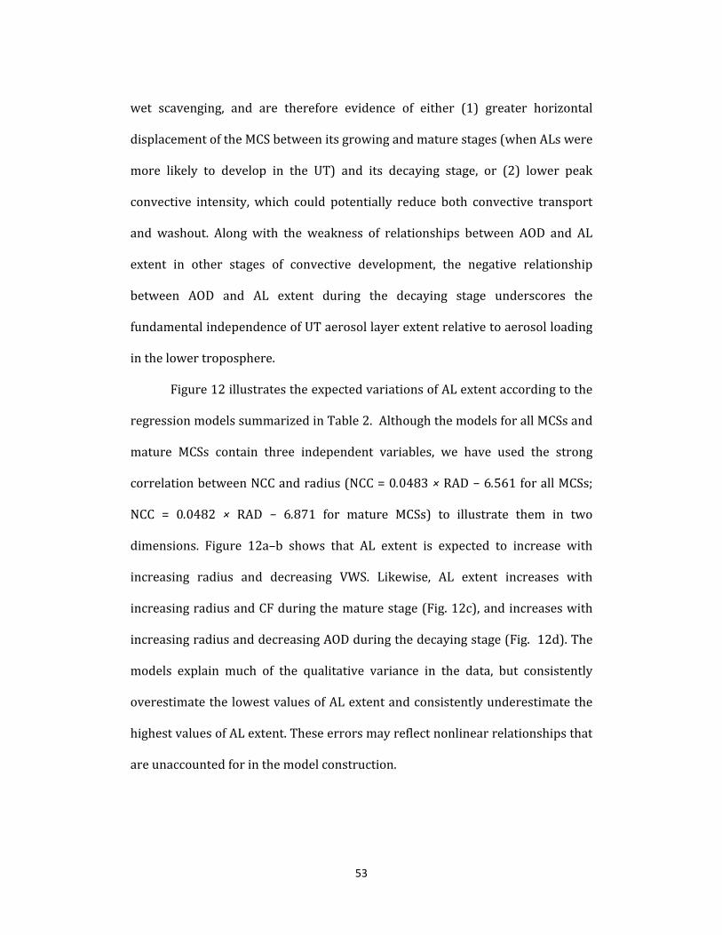
53

wet scavenging, and are therefore evidence of either (1) greater horizontal

displacementoftheMCSbetweenitsgrowingandmaturestages(whenALswere

more likely to develop in the UT) and its decaying stage, or (2) lower peak

convective intensity,which could potentially reduce both convective transport

and washout. Along with the weakness of relationships between AOD and AL

extent in other stages of convective development, the negative relationship

between AOD and AL extent during the decaying stage underscores the

fundamentalindependenceofUTaerosollayerextentrelativetoaerosolloading

inthelowertroposphere.

Figure12illustratestheexpectedvariationsofALextentaccordingtothe

regressionmodelssummarizedinTable2.AlthoughthemodelsforallMCSsand

mature MCSs contain three independent variables, we have used the strong

correlationbetweenNCCandradius(NCC=0.0483×RAD−6.561forallMCSs;

NCC = 0.0482 × RAD − 6.871 for mature MCSs) to illustrate them in two

dimensions. Figure 12a–b shows that AL extent is expected to increase with

increasing radius and decreasing VWS. Likewise, AL extent increases with

increasingradiusandCFduringthematurestage(Fig.12c),andincreaseswith

increasingradiusanddecreasingAODduringthedecayingstage(Fig.12d).The

models explain much of the qualitative variance in the data, but consistently

overestimatethelowestvaluesofALextentandconsistentlyunderestimatethe

highestvaluesofALextent.Theseerrorsmayreflectnonlinearrelationshipsthat

areunaccountedforinthemodelconstruction.

54

Figure12. Graphical representations of the statisticalmodels for (a) allMCSs,

(b)growingMCSs, (c)matureMCSs,and(d)decayingMCSs.Themodels forall

MCSs andmatureMCSshavebeen collapsed into twodimensionsbyusing the

strong linear correlation between radius andNCC (see text and Figures 8 and

10).Ascatterplotofthebinneddataforeachcaseisshownforreference,andthe

fractionof variance explainedby the linearmodel is shown at the top right of

eachpanel.

2.5.Summary

ThemorphologyanddynamicstructureofMCSsispotentiallycriticalfor

convectiveaerosoltransportthroughouttheirlifecycle,yetrelativelyfewstudies

haveevaluated therelationshipsbetween themorphologyofMCSsandaerosol

transportatthescalesoftropicalcontinents.Ouranalysisusesmultipleyearsof

satellite data to evaluate relation‐ ships between convective properties and

55

aerosoltransporttotheUToverthreedifferenttropicalregionsandduringthree

differentstagesofMCSdevelopment.

Manypreviousstudiesofaerosoltransporthavefocusedonvariationsin

UTCO,whichhasbeenusedasasurrogateforbiomassburningaerosols[Jianget

al., 2008]. Here,we have introduced an approach that combines ISCCP andA‐

Train satellite observations to explore the relationships between convective

characteristics and direct observations of aerosol layers in the nearby UT. A‐

Trainobservationsallowustoexaminethedetailedverticalstructureofclouds

andaerosollayersinthetropicalUT,whileISCCPdataprovidesvaluablecontext

with respect to both the large‐scale environment and the stage of convective

development.We focuson threestagesofconvectivedevelopment,whichhave

been defined according to changes in the area of the underlying MCS: the

growingstage, thematurestage,andthedecayingstage.Ourapproachyieldsa

sample of 963 MCSs covering three tropical regions: equatorial Africa, South

Asia, and the Amazon basin. This sample size is considerably larger than

previous attempts to infer relationships between convective properties and

aerosol transport, andallowsus todevelopmore robust statisticalmodels.We

find that thedynamic structureof convective systemsand the influenceof this

structureonaerosoltransportvarysignificantlyduringtheconvectivelifecycle.

Although it is generally expected that the magnitude and frequency of

convective aerosol transport are fundamentally tied to the strength of the

convection, our analysis represents the first attempt to characterize the

evolutionoftheserelationshipsthroughouttheMCSlifecycle.Aerosoltransport

isstrongestduringthegrowingstageofMCSdevelopmentoverSouthAsia,but

56

strongest during themature stage ofMCS development over equatorial Africa.

Thesedifferences are attributable to a combinationof (1) largerdifferences in

convective intensity between the growing and mature stages over equatorial

Africa than over South Asia and (2) the greater likelihood of diluted aerosol

concentrations during the mature stage due to scavenging by earlier

precipitation. GrowingMCSsarealmostequallyasstrongasmatureMCSsover

SouthAsia,butgrowingMCSsareconsiderablyweakerthanmatureMCSsover

equatorial Africa. The variation of convective aerosol transport frequency by

developmental stage is qualitatively similar over all three basins, but

convectively‐generated ALs are considerably less extensive over the Amazon

basin than over the other two regions. Rain rates are typically higher in

convectivesystemsovertheAmazonthaninconvectivesystemsoverSouthAsia

or equatorial Africa, which may enhance wet scavenging over the Amazon.

Moreover,convectivesizeandlifetimeareconsiderablyshorterovertheAmazon

thanoverSouthAsiaorequatorialAfrica,whichmaylimitaerosoltransport.

Our results show thatmuch of the variability in convectively‐generated

UTaerosollayers(ALs)canbeexplainedbyvariationsinthesize(radius)ofthe

MCS.ThisdependencedoesnotarisefromthedefinitionofALs,asALextentsare

calculatedoverthesamehorizontaldistancealongtheCALIPSOtrackregardless

of MCS size. The number of convective cores (NCC) is also identified as

influential in several cases, although its coefficient in the multiple regression

models isopposite insignto itscoefficient insingle‐variableregression.NCCis

stronglycorrelatedwithradius(R=0.92),andcarefulanalysissuggeststhatthe

primaryfunctionofNCCinthemodelistoaccountforregionalvariabilityinthe

57

relationship between radius andAL extent. Stronger vertical convective flux is

associatedwithalargernumberofconvectivecoresembeddedinaMCS,andthe

larger vertical flux leads to more aerosol being transported to the 10‐12 km

altitudelevels.

OptimalstatisticalmodelsrelatingconvectivepropertiestoALextentvary

considerablybybothregionandstageoftheconvectivelifecycle.Inparticular,

verticalwindshear(VWS)isrelatedtoALvariabilityduringthegrowingstage,

convectivefraction(CF)isrelatedtoALvariabilityduringthematurestage,and

aerosol optical depth is related to AL variability during the decaying stage.

Regional variability in several convective properties confounds physical

interpretationofthestatisticalrelationships.Thisconfusionmaybeparticularly

important for VWS,which receives a negative coefficientwhen all regions are

considered,butapositivecoefficientwhenonlySouthAsiaisconsidered.

Our analysis indicates that VWSmay play an important role in aerosol

transport during the growing stage. The VWS coefficient appears to act as a

surrogate for regionalvariabilitywhenall regionsareconsidered together,but

ALextentoverSouthAsiaincreasessignificantlywithincreasingVWS(R=0.30,

p = 0.03). A positive relationship between VWS and aerosol transport is

physically plausible, given the close relationship between convective and

boundarylayerpropertiesduringthegrowingstageandthepotentialforVWSto

enhance convective aerosol transport by establishing separate regions for up‐

drafts and downdrafts. Our results suggest that this physical interpretation is

most likely,butweareunable toconclusivelyruleoutalternativeexplanations

58

(suchassub‐regionalco‐variability inVWSandALextent). A fullevaluationof

thishypothesiswillrequiredetailedmodelsimulations.

Our statistical model results further indicate that mature systems with

similar sizeswill typically producemore extensive ALswhen the CF is larger.

This positive dependence on CF is only observed for mature systems. By

contrast, the extent of ALs associated with decaying systems is negatively

correlatedwithaerosolopticaldepth(AOD).Thisresultisintuitivelysurprising,

andmayreflectapositiverelationshipbetweenconvectiveaerosoltransportto

theUTandwetscavenging inthe lowertroposphereovertheprecedinghours.

WefindnosignificantcorrelationsbetweenAODandUTALextent,althoughwe

note thatouranalysis is restricted toMCSs thatoccurred inenvironments that

were at least somewhat polluted (i.e., at least some nearby pixelswith AOD≥

0.3).

Ourresultsprovidevaluablecontextregardingtherelativeimportanceof

different convectivepropertiesoverdifferent regionsandatdifferent stagesof

theconvectivelifecycle.Inparticular,wehaveidentifiedapotentiallyimportant

relationship between VWS and aerosol transport during the growing stage of

convectivedevelopment,andwehaveshownthatvariationsinALextentinthe

upper troposphereare largely independentof variations in lower‐tropospheric

AODabovethethresholdvalue.Theseresultsdemonstratethepotentialvalueof

ISCCP observations for developing deeper physical interpretations of the

detailed profiles of cloud and aerosol properties provided by the A‐Train

satellites,andprovideaninterpretiveframeworkforconstructingandevaluating

numericalmodelsimulationsofconvectiveaerosoltransport.

59

Chapter3

Relativeinfluenceofthemeteorologicalconditionsandaerosolsonthe

lifetimeofthemesoscaleconvectivesystems

3.1Introduction

Thehypothesis thataerosolsmaydelayprecipitationand increasecloud

lifetime of shallow marine clouds [Albrecht, 1989] has motivated many

researchers to study the aerosol indirect effect on convective clouds;however,

theinfluenceofaerosolsonenhancingcloudlifetimehasremainedunderdebate.

Mesoscale convective systems (MCSs) are deep convective clouds that cover

several hundred kilometers. Previous studies have shown that aerosols affect

deepconvection,inparticularthataerosolsincreasethenumberofsmallersize

cloud nuclei (CCN) [Rosenfeld andWoodley, 2000], which weaken coagulation

and coalescence that form raindroplets, and consequentlydelaywarmrainfall

[RosenfeldandLensky,1998;Rosenfeldetal.,2007].Theseprocessesallowmore

clouddropletstoriseabovethefreezinglevelandincreaselatentheatreleased

due to glaciation [Rosenfeld et al., 2008], resulting in stronger updraft speed,

enhanced cloud ice content [Linetal., 2006], larger anvil size [Rosenfeldetal.,

2008], and higher cloud top height [Koren et al., 2005]. The top of the

tropospherewarmsowing to the aerosol‐induced changes in convective anvils

[Koren et al., 2010b]. Although these aerosol effects have been seen in

observations from field campaigns [Bister and Kulmala, 2011; Lindsey and

Fromm, 2008], they have been undetectable on large spatial and multi‐year

60

scales.Rosenfeld etal. [2014b] have attributed this lack of detectability on the

large scale of aerosol invigoration of convection to its variation with

meteorologicalconditionsandtothelackofknowledgeoftherelativehumidity

(RH)outsidetheclouds.

The variation of aerosol effects on convection with meteorological

parametershasbeenstudiedpreviously[Rosenfeldetal.,2014b]. Forexample,

modelsimulationhasshownthatanincreaseinaerosolconcentrationsuptoan

optimallevelcaninvigoratetheMCSsunderweakverticalwindshear(VWS)and

higher relative humidity, but suppress the MCSs under strong VWS in a dry

environment[JWFanetal.,2007;JWFanetal.,2009].Theyfoundthatduetoa

significant enhancement in the convective available potential energy (CAPE),

corresponding to an increase in RH from 50% to 70%, aerosol impacts on ice

crystal mass becomes pronounced with a dramatic increase in the size of the

anvilsandthemassoficecrystalsofthedeepconvection.However,suchimpacts

arenegligiblewhenRHincreasesfrom40%to50%duetolittleincreaseinCAPE

[JW Fan et al., 2007].Moreover, consumption of CAPE for a given amount of

rainfall is converted to an equal amount of kinetic energy that invigorates the

convection [Rosenfeld, 2006;Rosenfeldetal., 2008].These studies indicate that

VWS,RH,andCAPEareimportantfactorsthatcaninfluenceaerosolimpactson

the MCSs. However, no quantitative assessment of the relative influence of

aerosols verses these meteorological parameters on convective lifetime using

satellitemeasurementshasbeenestablished[Rosenfeldetal.,2014b].

61

The influence of aerosols on theMCSs are expected to vary in different

phases of the convective life cycle. For example, Rosenfeld et al. [2008]

hypothesizedthattheimpactofaerosolondeepconvectionisstrongerandmore

prominentduring thedissipatingphase.Using cloud‐resolving simulations, JW

Fanetal.[2013]foundoutthataerosolmicrophysicaleffectsintensifythedeep

convectionduringthematureanddecayingphasesbyforminglargernumberof

smallerandlong‐lastingparticles,whereasadditionallatentheatreleaseddueto

aerosols’ thermodynamic effect is responsible for invigorating the deep

convectionsduring thegrowingphase.Hence, thedetectionof aerosol impacts

might may not be visible until the mature phase as no satellite can directly

measurethethermodynamicproperties.

Most of the above discussed studies were based on either model

simulations or limited case studies from field campaigns. Observational

assessments of how the influence of aerosols depend on meteorological

conditions and the convective life cycle, and whether aerosols could have a

significant influence on the lifetime of the MCSs at climate and large spatial

scales, have not been available [Rosenfeld etal., 2014b]. Stevensand Feingold

[2009] have suggested that climate models with parameterized cloud and

turbulence schemes tend to overestimate the effect of aerosols on clouds

compared to the models that resolve cloud processes and large eddies. The

extrapolationoftheresultsobtainedfromalimitednumberoffieldcampaignsto

global and climate scales is questionable. Hence, whether aerosols could

increase the lifetimeof theMCSson large spatial and climate scales, and if so,

62

howwouldsuchaneffectvarywithmeteorologicalconditionsandtheconvective

life cycle, has not been clear. Detection, measurement, and retrieval of the

aerosols properties from the satellite data in the vicinity of deep convective

cloudsatvariousstagesofacloud’slifecycleischallenging[Korenetal.,2010a].

Isolating the impact of aerosols from other meteorological conditions

observationallyrequireslargesamplesoftheMCSsundersimilarmeteorological

conditionsandatdifferentphasesoftheirlifecycle[Rosenfeldetal.,2014b].For

thispurpose,weuseasuiteofcollocatedgeostationaryandpolar‐orbitalsatellite

measurements, along with reanalysis products, constrained by both physical

principles intheatmosphericmodelandobservations, todeterminethephases

of MCSs’ lifecycle, lifetime, and ice water content of the MCSs and associated

ambient meteorological and aerosol conditions (See Methods). We examine

2430casesoftheMCSswithco‐locatedISCCPconvectivecloudsandMODISAOD

measurementstoestimatechangesofMCS’slifetimewithaerosolasafunctionof

changingmeteorologicalconditions.WeestimatechangesinMCS’slifetimewith

various meteorological parameters as a function of aerosol and other

meteorological parameters. We can also estimate the relative influences of

aerosolsandvariousmeteorologicalparametersonMCS’slifetimeusingmultiple

linearregressionatdifferentstagesoftheconvectivelifecycleandoverdifferent

regions.

63

3.2DataandMethods

Methods

WecollocateMODISand ISCCPdatasets to identify the convections that

are observed by different satellites between January 2003 and June 2008, in

ordertohavesufficientnumbersoftheMCSsneededforthestatisticalanalysis

used in this study. For South Asia, onlymonsoonmonths (June‐September) of

every year are considered. Domains of analysis, details of the collocation

techniqueandrelatederrorestimationprocessesaregiveninChakrabortyetal.

[2015]. Once a collocatedMCS is observed, we compute fAOD using theMODIS

AODpixels[Korenetal.,2008;JLeeetal.,2012;Livingstonetal.,2014;Rosenfeld

etal.,2008]withinanareaof2 latitude/longitudeinthevicinityofaMCS.We

determineMCSs’lifetime,phaseofconvectivelifecycle,anddifferentconvective

properties from the ISCCPDXdataset [Machadoetal., 1998], andcalculate the

CAPE, RH850, RH500, and VWS [Petersen et al., 2006] from the MERRA data

[Chakrabortyetal.,2015].Weintegratethemeanverticalreflectivityprofile(Z)

abovethefreezingleveltorepresentthecolumnarIWC[Matrosov,2009a]orIZ.

For details of the calculations and equations, please see the supporting

Information.Wehaveusedmultiple linear regressionstatistics [Chakrabortyet

al.,2015]basedonthelinearcombinationofthepredictors(CAPE,RH850,RH500,

VWS,andfAOD)toformasetofpredictiveequationstoestimatethevarianceof

MCSexplainedlifetime.

64

3.3ResultsandDiscussion

The lifetime of theMCSs is influenced by convective available potential

energy [Robert A. Houze, 1993; R. A. Houze, 2004; Mapes, 1993], an useful

measureforcloudbuoyancyandverticalvelocity[WilliamR.CottonandAnthes,

1989;Edward J.Zipser, 2003],moisture entrained from thewarmatmospheric

boundarylayer[WilliamR.CottonandAnthes,1989;RobertA.Houze,1993;R.A.

Houze,2004],andlateralentrainmentof freetroposphericmoisture,whichcan

dilute the buoyancy of the rising air and account for up to 33%‐50% of the

rainfall [Langhans et al., 2015]. VWS contributes to organizing the storms,

determiningwhetherupdraftanddowndraftregionsoverlap,slantwiseaccentof

themoist air, and precipitation [R.A.Houze, 2004;KingsmillandHouze, 1999;

Marwitz, 1972;Moncrieff, 1978;WeismanandRotunno, 2004].Weevaluate the

influenceofboththelowlevelVWS[Petersenetal.,2006;WeismanandRotunno,

2004] and the deep tropospheric VWS (see Methods). The former influences

rainfallandtotalcondensation[WeismanandRotunno,2004],whereasthelatter

influences vertical velocity [Weisman and Rotunno, 2004] and also MCS anvil

formation[Harrison,1992;Kilroyetal.,2014;Korenetal.,2010b;Petersenetal.,

2006;WeismanandRotunno,2004].

Past studieshave shown that the responseofdeep convective clouds to

aerosols is nonlinear. Over land, aerosol microphysical effects on deep

convective clouds saturate and reverse at AOD>0.3 [Koren et al., 2008].

Moderateconcentrationsofaerosols(orCCNs)maximizetheinvigorationeffect

of aerosols,whereashigher aerosol concentrations can reduce thevigorof the

65

convection[Rosenfeldetal.,2008].However,overhumidlandandoceans,more

aerosolisrequiredtosuppressrainfall.Thus,athresholdofAOD~0.3islikelyto

beoptimalasathresholdofpollutiontodeterminetheinfluenceofaerosolson

theMCSs[JLeeetal.,2012;Livingstonetal.,2014].WeuseAOD>0.15overland

andAOD>0.3overtheoceanasthethresholdforapollutedenvironment.

To isolate theeffect of aerosolsonMCSs’ lifetimeandcompare it to the

effectof theseprimarymeteorologicalconditions,weevaluatehowthe lifetime

oftheMCSschangeswithonestandarddeviation(1σ)ofCAPE,relativehumidity

at850hPa(~1.5kmabove thesea level,RH850), relativehumidityat500hPa

(~5.5 km above the sea level, RH500), deep tropospheric vertical wind shear

(VWS),andthefractionofthenumberofaerosolpixelswithAOD(fAOD)greater

than0.15(0.3)overland(theocean)tothetotalnumberofAODpixelswithina

rangeof2latitude/longitudefromtheboundaryoftheMCSs,respectively,over

allthreeregions(seeMethodsandSupportingInformation).Ouranalysisshows

thatusingAOD>0.3asathresholdforpollutedenvironmentoverbothlandand

oceandoesnot significantly change the influenceof aerosols onMCSs’ lifetime

(Fig.18). Also, theMCSs’ lifetime isnotsignificantlycorrelatedwith the lower

troposphericVWS(Fig.17).Moreover,responseofMCSlifetimetoa1σincrease

in CAPE is weaker when we consider lower tropospheric VWS (Figs. 17c and

17d),comparedtothatundertheinfluenceofdeepVWS(Fig13a).Thus,weshow

ourresultsinthemainbodyofthisworkusingAOD>0.15asthethresholdfora

polluted environment over land, and AOD>0.3 as the threshold for a polluted

environmentoverocean,andalsoshowresultsfordeeptroposphericVWS.

66

These abovementioned conditions are determined by the International

Satellite Cloud Climatology Project convective tracking, Moderate Resolution

ImagingSpectroradiometer(MODIS),andtheModern‐EraRetrospectiveanalysis

forResearchandApplications(MERRA)datasets.Ourcalculationsontheglobal

tropical continental scale indicate that MCSs’ lifetime increases at the highest

rates with an increase of CAPE under intermediate to high VWS values and

pollutedconditions.MCS’slifetimeincreasesabout3‐30hoursforanincreaseof

CAPEbyone standarddeviation (1σ, Fig. 13a). Themultiple linear regression

(Fig. 13f) also shows that CAPE explains 33% of the total variance of MCSs’

lifetime,largerthananyothermeteorologicalandaerosolconditions.RH850isthe

secondmostinfluentialparameteronMCSs’lifetime,explaining27%ofitstotal

variance (Fig.13b). MCS’s lifetime increases by 3‐27 hours per 1σ increase of

RH850 under intermediate to high VWS values and polluted conditions. The

lifetimeof theMCSs also increaseswithRH500 by 3‐9 hours for 1σ increase of

RH500 under polluted conditions (Fig. 13c), explaining only 4% of the total

variance of MCSs’ lifetime. MCSs’ lifetime decreases by 6‐9 hours for a 1σ

increaseofVWSindryenvironmentswithlowfAODvalues,butincreasesby3–30

hours for a 1σ increase of VWS in the high RH850 environment. Overall, VWS

explains16%of the total varianceof the lifetimeofMCSs. It is the thirdmost

influentialmeteorologicalconditiononMCCs’ lifetime. Inaddition, increases in

MCS lifetime with other meteorological and aerosol conditions (CAPE, RH850,

RH500 and fAOD, respectively) are stronger at moderate to high level of VWS

(Figures13a,13b,13c,13d, and13e),possiblybecauseprecipitationefficiency

decreasesbelow50%whenVWSisabove20x10‐4S‐1[Marwitz,1972],whereas

67

weak tomoderateVWS isassociatedwithheavyconvectiverainfall [WilliamR.

CottonandAnthes,1989;Maddoxetal.,1979].

ThelifetimeofMCSsappearstoincreasewithaerosolsby3‐15hourswith

1σ increase of fAOD but only under highRH850 andmoderate to highVWS (Fig.

13d).MCS’slifetimedecreaseswithfAODunderlowerRH850by3‐6hoursper1σ

increase of fAOD. MCSs’ lifetime increases with fAOD by 3‐24 hours under high

valuesofCAPEandmoderatetohighvaluesofVWS(Fig.13e)andalsodecreases

atlowvaluesofCAPEandVWSattherateof3‐6hoursdueto1σincreaseoffAOD.

Overall,fAODexplainslessthan1%ofthetotalvarianceofMCSs’lifetime.Thus,on

thescaleofglobaltropicalcontinents,thelifetimeoftheMCSsismainlylinkedto

meteorological conditions anddominatedby theCAPEand lower tropospheric

humidity, which is consistent with previous studies [William R. Cotton and

Anthes,1989;DelGenioandWu,2010;R.A.Houze,2004;Langhansetal.,2015;

Mapes,1993].TheseresultsdonotvarysignificantlyforfAODusingtheAOD>0.3

insteadofAOD>0.15asthethresholdforpollutedenvironmentoverland(Fig.13

andFig.18).

However,theaerosolinfluenceonMCSs’lifetime,cloudicewatercontent,

andconvectiveanvilsmaynotbecomedetectablebysatellitesuntil themature

or decay phases, as the available satellite sensors cannot effectively detect

changesofcloudparticlesizechangeinthelowerandmiddletroposphereinside

ofconvectionandcloudthermodynamiceffects.Thus,weseparatelyanalyzethe

variationsofMCSs’lifetimewithambientconditionsduringthegrowing,mature,

anddecayphases,respectively.Figures14a‐14cshowsthatCAPEdominatesthe

68

variance ofMCSs’ lifetime during the growing phase, explains 36% of its total

variance, but become less influential during the mature and decay phases,

explaining25%,and9%ofthetotalvariance,respectively.RH850dominatesthe

varianceofMCSs’lifetimeduringthematureanddecayphases,explaining46%

and44%of the total variance, respectively. VWSexplains about4‐34%of the

total variance of the durations of these phases. The dominant influence of

relative humidity and CAPE over VWS reflects mainly the large geographic

variations of MCSs’ lifetime with the ambient atmospheric humidity that is

neededtosustaintheMCSs.Incomparison,aerosolsexplain6%and24%ofthe

totalvarianceofthematureanddecayphaselongevity,respectively,anddonot

appeartohavedetectableinfluenceonthedurationofthegrowingphaseofthe

MCSs.

Are the empirical relationships between MCSs’ lifetime and ambient

meteorological and aerosol conditions shown above physically reasonable?

Based on the hypothesized underlying mechanism of aerosol influence on

convectivelifetime,anincreaseinMCSs’ lifetimeisdueto increaseofcloudice,

especially intheformofsmallercloudparticlesabovethe freezing levelwithin

convectivecoresandanvils. Sucheffectsmaybemoreapparentanddetectable

by satellite sensors, as slower sedimentation of larger amount of smaller ice

particles can sustain convective anvils for longer time. Thus, we analyze the

vertically integrated cloud ice content of the MCSs (IZ, See Methods and

Supporting Information) derived from CloudSat (Figs. 14d‐14f) and ice water

contentat216hPa(~12kmabovethesealevel, IWC_216)ofconvectiveanvils

69

from theAuraMicrowaveLimbSounder (MLS)datasetsbasedon966casesof

theMCSs (over the limited period of June 2006 for CloudSat to June 2008 for

ISCCP‐DX)with co‐located ISCCP, CloudSat, andMLSmeasurements in Figures

14d‐14i. Notice that IZ represents the mass of larger ice particles above the

freezinglevel(above5km)mainlywithintheconvectivecoresandlowerportion

oftheanvils,whereasIWC_216representsthemassofsmallerparticlesneartop

of the convective anvil. Hence, their relationships with meteorological and

aerosolconditionscanbedifferent.

Figures 14d shows that IZ’s variance is primarily explained by RH850

(43%)andCAPE(39%)duringthegrowingphase.VWSexplains12%ofthetotal

variance of the IZ (Fig. 14d). The result is broadly expected based on the

controllingfactorsofconvectionreportedintheliterature[WilliamR.Cottonand

Anthes, 1989; Robert A. Houze, 1993; R. A. Houze, 2004; Mapes, 1993]. The

varianceof thecloud ice in theconvectiveanvil (IWC_216,Fig.14g)during the

growing phase is explained mostly by CAPE, presumably because convective

detrainment in the upper troposphere or anvils generally increases with

buoyancy. During thematurephase,CAPEandVWSexplains57%and14%of

thetotalvarianceoftheIZ,respectively(Fig.14e),presumablybecauseoftheir

influenceonconvectivemassfluxabovethefreezinglevel.Incontrast,RH850and

fAOD appear to be most influential on the ice water content of the anvils,

explaining64%and26%ofitstotalvariance,respectively,presumablybecause

oftheirstronginfluenceontheamountandeffectivesizeofsmallericeparticles

[JW Fan et al., 2013]. During the decay phase, CAPE and fAOD dominate the

70

variance of IZ, explaining 51%and35%of its total variance, respectively. fAOD

dominatestheIWC_216variation,explaining27%ofitstotalvariance.VWSand

RH500 also have significant influence on IWC_216; each explaining 11% of the

totalvarianceinthedecayphase.Suchincreasinginfluencesofaerosols,middle

tropospheric humidity and deep tropospheric vertical wind shear are also

physically plausible as theMCSs at decay phase become increasingly detached

fromthelowertroposphere.

The analysis of these independently measured variables in Fig. 14

suggests a stronger influence of aerosols on the duration of the MCSs’ decay

phase, probably due to the stronger influence of aerosols on cloud ice water

contentinbothconvectivecoresandanvilsduringthisphase.CAPE,RH850,and

VWSdominatetheexplanationofvarianceofMCS’slifetime,icewatercontentof

the convective cores and anvils during the growing and mature phases.

Generally, aerosols have a stronger influence on convective anvils than on ice

watercontentofconvectivecoresandMCSslifetime,presumablybecauseofthe

formationoflargernumberofsmallericeparticles[JWFanetal.,2013],which

are sensitive to aerosol loading. The smaller ice particles are more likely

suspended in convective anvils, and thus can influence the anvil ice water

contentandlifetime.

Figure 15 shows the relative influences of ambient aerosols versus

meteorological conditions onMCSs’ lifetimewithin each continent. Figure 15a

shows that meteorological parameters explain approximately 92% and fAOD

explainsupto8%ofthetotalvarianceofthelifetimeoftheMCSsoverequatorial

71

Africa.OverSouthAsia,only39%ofthetotalvarianceoftheMCSs’lifetimecan

beexplainedbymeteorologicalandaerosolconditionswhenweconsiderallthe

MCSs(Fig.19). However,wefoundthat45%oftheMCSsformedandmatured

overtheIndianOcean,BayofBengal,andArabianSea(Fig.16c).Evaluatingthe

relationship between these MCSs when they were over the ocean and the

associated ambient meteorological conditions and fAOD (using AOD>0.3 as the

threshold),we findthatRH850dominates the lifetimeof theseMCSs,explaining

about45%of the totalvariance; fAODalsohasan important impact, explaining

~20%ofthetotalvariance(Fig.15b).RH500andVWSexplain15%and12%of

the total variance, respectively. What causes the large fraction of the

unexplainablevarianceoftheMCSs’overIndiancontinentremainsunclear.

The dominantMCSs’ type and aerosol conditions over equatorial South

America are sharply different between the wet (December to April) and dry

(June to September) seasons. Thus, we separately evaluate the influences of

meteorological and aerosol conditions on theMCSs for the dry orwet season.

CAPE, VWS and fAOD explain ~31%, ~29%, and ~20% of the total variance of

MCSs’ lifetime during the dry season (Fig. 15c), respectively, suggesting a

comparable rolebetween these threevariables. AmbientRH500alsoexplainsa

significant fraction of lifetime variance, likely because the drier middle

troposphere isastronger limiting factor for theoccurrenceofMCSsduring the

dryseasonthaninthewetseasonoverequatorialSouthAmerica[WHLiandFu,

2006]. During thewet season, CAPEand fAOD explain~41%and~22%of the

total variance, respectively. The link between relative humidity and MCSs’

72

lifetime in South America is weaker compared to other tropical continents,

presumably because humidity is not as strong a limiting fact as in the drier

continents(Fig.16b).

Could different meteorological conditions explain variations of the

relativeenvironmental influenceson theMCSsbetweendifferentphasesof the

convectivelifecycleandthethreetropicalregions?Figure16ashowsthataerosol

concentrations and meteorological conditions do not change significantly

between the threephasesof theMCSs’ lifecycle.Thus, thedecreaseof the total

varianceexplainedbymeteorologicalconditionsisunlikelytobecausedbytheir

changesduringtheMCSs’lifetime.Theincreasedfractionofthetotalvarianceof

MCSs’ lifetimeexplainedbyaerosolsduring thedecayphase is consistentwith

numericalmodelsimulations[JWFanetal.,2013;LohmannandFeichter,2005]

andsupportsthecloudlifetimeenhancementbytheaerosolsduringthatphase.

This can be explained by the significant fraction of the variance of ice content

inside the convective core and smaller cloud particles in convective anvils

explainedby fAOD.Theseeffectscouldreducesedimentationof iceparticlesand

dissipationofconvectiveanvils.Wecannotruleoutaninfluenceofthereduced

backgroundaerosol loadingon lifetime [Rosenfeldetal., 2008;VanDenHeever

andCotton,2007].

Figure16bshowsthatequatorialAfricaisthedriestregionandhashighly

variablerelativehumidity in the lowandmiddle troposphere,asshownby the

means and standard deviations of the RH850 and RH500. The region also has

relativelylowVWS,butisrichinaerosols(fAOD).Thus,moistureavailabilitycould

73

betheprimarylimitingfactorforlifetimeoftheMCSs[R.A.Houze,2004]andthe

RH850 andRH500 together explain about 70%of their total variance. TheMCSs

over equatorial South America are surrounded by the lowest fAOD (when we

considerfAODoverthelandsectorsofallthreeregions)andVWS(Fig.16b)and

the highest amount of RH850. Such favorable meteorological (Fig. 13b) and

aerosol conditions may explain stronger connection between fAOD and MCSs'

lifetimeoverSouthAmerica(Figs.15cand15d)thanthoseoverequatorialAfrica

andSouthAsia. Inaddition,MCSsoverequatorialSouthAmericaaresmaller in

size (mean radius ~168 km), have lesser numbers of convective cores (mean

NCC~3)andshorterlifetime(<20hours)comparedtothoseofequatorialAfrica

(mean radius~440km,37hours, andmeanNCC~10) and southAsia (mean

radius~490 km, 120 hours, and mean NCC ~ 9). The combination of these

meteorological, aerosol conditions, and MCSs’ structures may contribute to

strongerinfluenceofaerosolsonthoseMCSsoverequatorialSouthAmerica.

OvertheIndianOcean,BayofBengal,andArabianSea,fAODthatsurrounds

theMCSsover theocean is 35% less than that over the land.ThemeanCAPE,

RH500, and deep level VWS associated with the MCSs over the ocean are the

strongestamongalltheregions.MeanCAPEoverlandis(~860J/kg)lowerthan

that over the ocean, consistent with previous findings based on reanalysis

[Riemann‐Campeetal.,2009]andmeteorologicalstation’sdatasets[Bhowmiket

al.,2008].RH850associatedwiththeMCSsovertheoceanicsurface isalsohigh.

Based on Fig. 13, such meteorological conditions favor a stronger increase of

MCSs lifetime with fAOD. Figure 16c shows the mean and variability (standard

74

deviation) of theMCSs’ lifetime over the three regions of our analysis and the

adjacentoceans.TheMCSsoverSouthAsiahavethelongestlifetime,onaverage

120hours,whichisthreetimestheaveragelifetimeoftheMCSsoverequatorial

Africa(37hours)andsixtimesofthatoverequatorialSouthAmerica(19hours).

Only 55%of theMCSs over south Asia originally form over the land,whereas

about80‐90%of theMCSsoriginatedfromlandoverequatorialSouthAmerica

andequatorialAfrica.Moreover,whenweconsideralltheMCSs,wefindthatthe

mean lifetimeof convection (irrespective ofwhether it originates over land or

ocean)over the land(orangebar) isapproximatelyhalfof the timeconvection

spendsovertheocean(bluebar).Inotherwords,45%ofthesystemsthatendup

decayingoverthelandspendmuchoftheirlifetimeovertheocean.

Throughoutouranalysis, fAODexplainshigh fractionsof totalvarianceof

theMCSs’ lifetimewhenfAODvaluesare low, forexample,overequatorialSouth

America(with the lowestcontinental fAODoverall theregions),over the Indian

Ocean,BayofBengal,andArabianSea,andduringthedecayingstage.

Many environmental parameters, such as the CAPE [Robert A. Houze,

1993;R.A.Houze, 2004;Mapes, 1993;Edward J.Zipser, 2003] , RH [WilliamR.

CottonandAnthes,1989;JWFanetal.,2007;RobertA.Houze,1993;Langhanset

al., 2015], andVWS [WilliamR.CottonandAnthes, 1989; JWFan etal., 2009;

Maddox et al., 1979; Petersen et al., 2006;Weisman and Rotunno, 2004], have

beenknowntoinfluenceMCSslifetime. However, toourknowledge,this isthe

first satellite based global tropical continental scale assessment of the relative

rolesofmeteorologicalconditionsversusaerosolsindeterminingthevariations

75

of cloud ice and lifetime of the MCSs using collocated geostationary, a set of

closely synchronized polar orbital satellites as part of the A‐train satellite

constellation, and MERRA reanalysis datasets on MCSs’ lifetime. These results

show that aerosol can either increase MCSs’ lifetime under higher relative

humidity, CAPE, andmoderate‐high deep tropospheric vertical wind shear, or

decreaseMCSs’ lifetime under lower relative humidity, CAPE, and low vertical

windshear.Ontheglobaltropicalcontinentalscale,anincreaseinMCSs’lifetime

with aerosol are most apparent during the decay phase, presumably by

increasingtheicewatercontentofconvectiveanvilsandconvectivecores.Such

a dependence of the aerosol effect on specific meteorological conditions and

phases of theMCS’s lifecycle presumably explains the difficulty of establishing

aerosol effects on global scale with its large variations to meteorological

conditions.Italsoappearstobroadlyexplainastrongerinfluenceofaerosolson

MCSs’ lifetime in humid equatorial South America during the wet season and

over the Indian Ocean/Bay Bengal with lower aerosol loading, versus the

relativelydryconditionswithhigheraerosol loadingoverequatorialAfricaand

dry season South America. Thus, the approach developed in this study can

potentiallyprovideakeytoreconcilethedifferencesoftheaerosoleffectsonthe

MCSsreportedinvariousliterature.

MCSsproduceheavyrainfallandthustheir lifetimeshouldbe important

fordeterminingrainfall/floodanddiabaticheatingforatmosphericcirculations.

Yet, our understanding of aerosol impacts on MCSs’ lifetime has been very

limited in large part due to lack of adequate long term observations on large

76

scales.ThelargesamplesoftheMCSsobservedbyasuiteofsatellitesensorsover

global tropical continents have enabled us to evaluate aerosol effects during

different phases of MCSs lifecycle under similarmeteorological conditions. In

doing so, this work has advanced our capability to evaluate whether or not

aerosols can increase convective lifetimes on the climate scale and to identify

what are the favorable meteorological conditions for aerosols to affect the

lifetimeoftheMCSs.Thesearefundamentalquestionsthathavemotivatedmany

studiesfordecades.However,wedidnotaddresstheinfluenceofdifferenttypes

of aerosols (such as absorbing or scattering) on MCSs’ lifetime, nor directly

observe the effect of aerosols on cloudmicrophysics. Use of aerosol type data

frominsitumeasurements,Cloud‐AerosolLidarandInfraredPathfinderSatellite

Observation (CALIOP data) as well as aerosol index data from the Ozone

MonitoringInstrument(OMI)alongwithgroundbasedmeasurementscouldbe

thenextsteptoaddresstheselimitations.

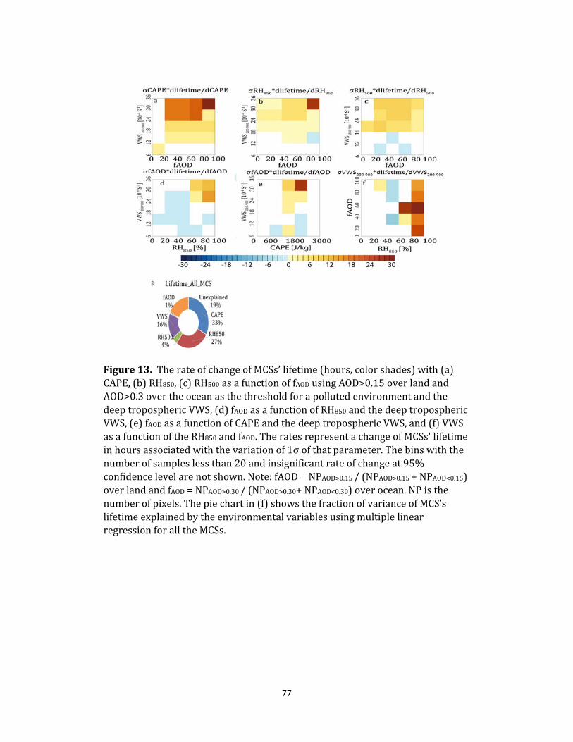
77

Figure13.TherateofchangeofMCSs’lifetime(hours,colorshades)with(a)CAPE,(b)RH850,(c)RH500asafunctionoffAODusingAOD>0.15overlandandAOD>0.3overtheoceanasthethresholdforapollutedenvironmentandthedeeptroposphericVWS,(d)fAODasafunctionofRH850andthedeeptroposphericVWS,(e)fAODasafunctionofCAPEandthedeeptroposphericVWS,and(f)VWSasafunctionoftheRH850andfAOD.TheratesrepresentachangeofMCSs'lifetimeinhoursassociatedwiththevariationof1σofthatparameter.Thebinswiththenumberofsampleslessthan20andinsignificantrateofchangeat95%confidencelevelarenotshown.Note:fAOD=NPAOD>0.15/(NPAOD>0.15+NPAOD<0.15)overlandandfAOD=NPAOD>0.30/(NPAOD>0.30+NPAOD<0.30)overocean.NPisthenumberofpixels.Thepiechartin(f)showsthefractionofvarianceofMCS’slifetimeexplainedbytheenvironmentalvariablesusingmultiplelinearregressionforalltheMCSs.

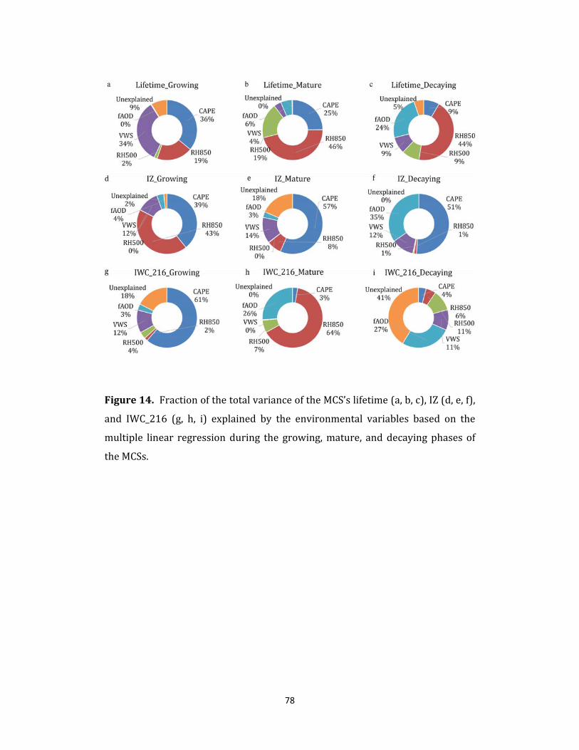
78

Figure14.FractionofthetotalvarianceoftheMCS’slifetime(a,b,c),IZ(d,e,f),

and IWC_216 (g, h, i) explained by the environmental variables based on the

multiple linear regression during the growing,mature, and decaying phases of

theMCSs.

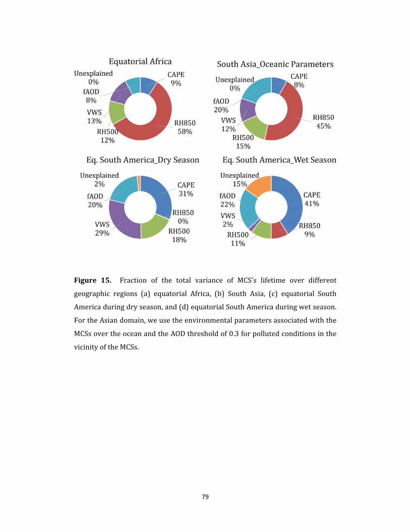
79

Figure 15. Fraction of the total variance of MCS’s lifetime over different

geographic regions (a) equatorial Africa, (b) South Asia, (c) equatorial South

Americaduringdryseason,and(d)equatorialSouthAmericaduringwetseason.

FortheAsiandomain,weusetheenvironmentalparametersassociatedwiththe

MCSsovertheoceanandtheAODthresholdof0.3forpollutedconditionsinthe

vicinityoftheMCSs.

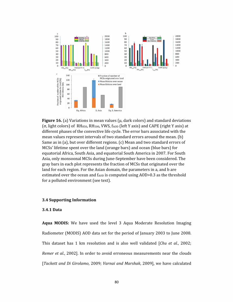
80

Figure16.(a)Variationsinmeanvalues(μ,darkcolors)andstandarddeviations(σ,lightcolors)ofRH850,RH500,VWS,fAOD(leftYaxis)andCAPE(rightYaxis)atdifferentphasesoftheconvectivelifecycle.Theerrorbarsassociatedwiththemeanvaluesrepresentintervalsoftwostandarderrorsaroundthemean.(b)Sameasin(a),butoverdifferentregions.(c)MeanandtwostandarderrorsofMCSs’lifetimespentovertheland(orangebars)andocean(bluebars)forequatorialAfrica,SouthAsia,andequatorialSouthAmericain2007.ForSouthAsia,onlymonsoonalMCSsduringJune‐Septemberhavebeenconsidered.ThegraybarsineachplotrepresentsthefractionofMCSsthatoriginatedoverthelandforeachregion.FortheAsiandomain,theparametersina,andbareestimatedovertheoceanandfAODiscomputedusingAOD>0.3asthethresholdforapollutedenvironment(seetext).

3.4SupportingInformation

3.4.1Data

AquaMODIS: We have used the level 3 Aqua Moderate Resolution Imaging

Radiometer(MODIS)AODdatasetfortheperiodofJanuary2003toJune2008.

This dataset has 1 km resolution and is also well validated [Chu et al., 2002;

Remeretal.,2002]. Inordertoavoiderroneousmeasurementsneartheclouds

[TackettandDiGirolamo,2009;VarnaiandMarshak,2009],wehavecalculated

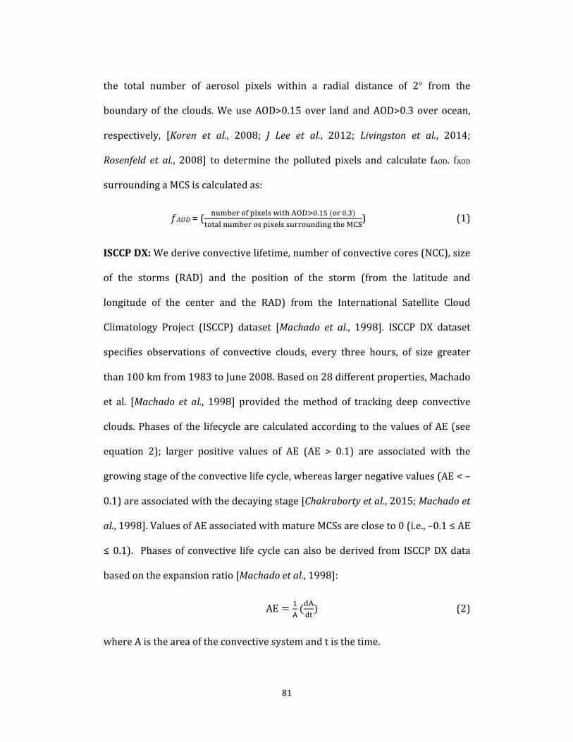
81

the total number of aerosol pixels within a radial distance of 2° from the

boundaryof the clouds.WeuseAOD>0.15over land andAOD>0.3over ocean,

respectively, [Koren et al., 2008; J Lee et al., 2012; Livingston et al., 2014;

Rosenfeld etal., 2008] to determine the polluted pixels and calculate fAOD. fAOD

surroundingaMCSiscalculatedas:

=( . .

) (1)

ISCCPDX:Wederiveconvectivelifetime,numberofconvectivecores(NCC),size

of the storms (RAD) and the position of the storm (from the latitude and

longitude of the center and the RAD) from the International Satellite Cloud

Climatology Project (ISCCP) dataset [Machado et al., 1998]. ISCCP DX dataset

specifies observations of convective clouds, every three hours, of size greater

than100kmfrom1983toJune2008.Basedon28differentproperties,Machado

et al. [Machado etal., 1998] provided themethod of tracking deep convective

clouds.Phasesof the lifecyclearecalculatedaccording to thevaluesofAE(see

equation 2); larger positive values of AE (AE > 0.1) are associated with the

growingstageoftheconvectivelifecycle,whereaslargernegativevalues(AE<–

0.1)areassociatedwiththedecayingstage[Chakrabortyetal.,2015;Machadoet

al.,1998].ValuesofAEassociatedwithmatureMCSsarecloseto0(i.e.,–0.1≤AE

≤0.1). Phasesof convective life cycle canalsobederived from ISCCPDXdata

basedontheexpansionratio[Machadoetal.,1998]:

AE (2)

whereAistheareaoftheconvectivesystemandtisthetime.

82

MERRA:WealsousetheModernEraRetrospective–AnalysisforResearchand

Applications (MERRA) data sets to calculate the RH850 and RH500 in order to

estimatethelowlevelandmid‐levelhumidity.SinceMERRAalsoprovidesdata

at3and6hourintervals,weusethedataprovidedintheISCCPdatasettolocate

thepositionsandboundariesoftheMCSsintheMERRAdataandcalculateRHat

a radial distance of 2° from the boundary of the clouds at two levels. VWS

associatedwitheachMCSiscalculatedasthedifferencebetweenthemeanwind

speeds of the layers 925‐850 hPa and200‐200 hPa[Petersen etal., 2006]. It is

thendividedbythedifferencebetweenthemeangeopotentialheights(∂z)ofthe

layersused(seeequation3).ForlowlevelVWSwetakethedifferencesinmean

wind speedandgeopotential heightbetween the layers950‐900hPaand750‐

700hPa.WecalculateVWSfromMERRAdata:

VWS

(3)

where ∂u is the change inmean zonal wind speed and ∂z is the difference in

meangeopotentialheightbetweenthe925–850hPaand250‐200hPalayersfor

the deep tropospheric VWS, and between the 950‐900 hPa and 750‐700 hPa

layers [Petersenetal., 2006] for the low troposphericVWS.WecalculateCAPE

betweentheleveloffreeconvectiontothelevelofnobuoyancyusingthespecific

humidity(then,convertedtomixingratio)andthetemperaturedatasets forall

thegridcellsundertheMCSs.

83

CloudSat: CloudSat has a wavelength of 3 millimeter [Langenberg, 2005] and

measuresthepowerbackscatteredbythecloudsasafunctionofdistancefrom

theradar[Stephensetal.,2002].Thedatahaveaverticalresolutionof240mand

horizontal resolution of 1.4 km (across track) x 1.7 km (along‐track). We use

radar backscatter profile (2B‐GEOPROF) datawith good quality (quality index

equalto0).Thevalidrangeofdetectionis‐40to50dBZ.Weusethereflectivity

data to represent the cloud icewater content rather than the retrieved values

derived from the reflectivity data. We compute IZ for the collocated MCSs

between CloudSat, MODIS, and ISCCP between June 2006 to June 2008 since

CloudSat datasets are available since June2006. From the reflectivity data,we

firstcalculatethemeanverticalreflectivity(Z)profileforeachoftheco‐located

MCSs.Figure20showsatypicalmeanreflectivityprofileofaMCS. Thelevelof

maximumreflectivitydenotes the freezing levelor themelting layerdueto the

melting hydrometeors [Matrosov, 2009a; b;Matrosov et al., 2007]. Under the

freezing level, the rain layer decreases the reflectivity due to the attenuation

[Matrosov, 2007]. We integrate themean reflectivity above the freezing level

with height to derive IZ (see equation 4). We integrate the mean vertical

reflectivityprofile (IZ) above the freezing level to represent the columnar IWC

[Matrosov,2009a]as:

IZ Zdh (4)

wherehistheheightinkm.

AURA MLS: We also use version 3.3 Aura Microwave Limb Sounder (MLS)

retrievalsofIWCtoestimatethechangesintheanvilIWCduetoaerosolsat216

84

hPa.Wehave applied the “2σ− 3σ” screeningprocess [Livesey etal., 2013] to

eliminatetheuncertaintiesduetotheeffectsofspectroscopicandcalibrationby

removingIWCretrievals thatare lessthanthreestandarddeviationsabovethe

meanin10°latitudebands.Asouranalysisislimitedoverthetropicalregion,we

excludethepossibilityofuncertaintiesinIWCduetogravitywavesoriginatingin

thewintertimestratosphereovermiddle‐to‐highlatitudesduringwintertime.To

be consistentwith IZ analysis fromCloudSat,we also analyzeMCSs collocated

betweenJune2006toJune2008.

3.4.2Statisticalmethods

InadditiontoestimatetherateofchangeofMCS’slifetimewithavariationofone

standard deviation of CAPE, RH, and VWS (both low and deep level), we also

apply a multiple linear regression method. In this method, the fraction of

varianceoftheMCSs’ lifetimeexplainedbydifferentmeteorologicalparameters

and aerosols is estimated. The dependent variable (here, MCSs’ lifetime) is

statisticallymodeledasalinearcombinationofindependentvariables:

β ∑ (5)

whereβistheinterceptandβj,j€[1,p]isthecoefficientassociatedwiththejthof

p predictors for the dependent variable yi. In this paper, we use traditional

methods formultiple linear regression that selects the coefficients in order to

minimizetheresidualsumofsquaresforNnumberofruns:

∑ ∑ (6)

85

Themethodofcollocatingcontainsmanypotentialsourcesofrandomerror.One

suchsourceisthemeasurementuncertaintyduetothedifferencesinthepartof

theMCSsthesatellitesobserve.Forexample,aCloudSatswathcanpassthrough

thecenteraswellasthroughtheedgeofthecloud.Tocounteractthisproblem,

wefirstsortthedatainincreasingorderofconvectivelifetime.Wethenbinthe

predictors (CAPE, RH850, RH500, VWS, fAOD; ) and the dependent variable

(convective lifetime; ) and construct a model based on multiple linear

regressionmethods.Startingwith10samples,wegraduallyincreasethenumber

of samples in eachbin andeach time,weobtainamodelwith residual sumof

squares (equation6), coefficients ( )associatedwithdifferentpredictors, and

varianceofMCSslifetimeexplainedbythem.Givenasetofthe5predictors,our

objectiveistoidentifyalinethatbestfitsthepoints.Inotherwords,theoptimal

model is chosen based on the minimum value of residual sum of square. We

report the explained variance of convective lifetime by different predictors

correspondingtothatoptimalmodel.

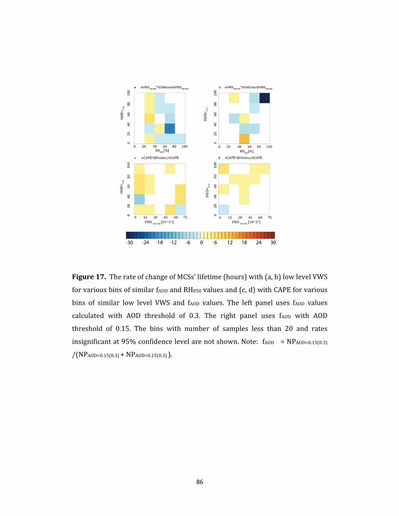
86

Figure17.TherateofchangeofMCSs’lifetime(hours)with(a,b)lowlevelVWS

forvariousbinsofsimilarfAODandRH850valuesand(c,d)withCAPEforvarious

bins of similar low level VWS and fAOD values. The left panel uses fAOD values

calculated with AOD threshold of 0.3. The right panel uses fAOD with AOD

threshold of 0.15. The bins with number of samples less than 20 and rates

insignificantat95%confidencelevelarenotshown.Note:fAOD=NPAOD>0.15(0.3)

/(NPAOD>0.15(0.3)+NPAOD<0.15(0.3)).

87

Figure18. (a)TherateofchangeofMCSs’ lifetime(hours)withonestandard

deviationof fAOD(0.3astheAODthresholdforpollutedpixels)asa functionof

deeptroposphericVWS.andRH850.(b)TherateofchangeofMCSs’lifetimewith

onestandarddeviationofCAPEasafunctionofdeeptroposphericVWS.andfAOD

(0.3astheAODthresholdforpollutedpixels).Thebinswithnumberofsamples

lessthan20andratesinsignificantat95%confidencelevelarenotshown.

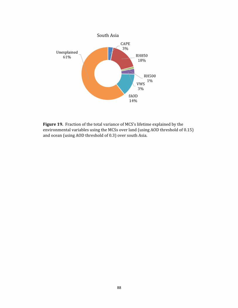
88

Figure19.FractionofthetotalvarianceofMCS’slifetimeexplainedbytheenvironmentalvariablesusingtheMCSsoverland(usingAODthresholdof0.15)andocean(usingAODthresholdof0.3)oversouthAsia.

89

Figure20.IZrepresentstheverticalintegratedradarreflectivityabovethefreezinglevelusingatypicalreflectivityprofileofaMCSasmeasuredbytheWbandcloudradar.

90

Chapter4

Relativeinfluenceofthemeteorologicalandaerosolconditionsonthe

mesoscaleconvectivesystemsthroughtheirlifecycleovertropical

continents

4.1.Introduction

Mesoscale convective systems (MCSs) with hundreds of kilometers in

radiusand lastingat least sixhoursareaprimary sourceofprecipitationover

the tropics and mid‐latitudes [R. A. Houze, 2004] and have disproportionally

largeinfluenceonthevariabilityoftheextremerainfallevents,suchasfloodand

droughts[R.A.Houzeetal.,2015].Paststudieshavesuggestedthattheintensity

andlifecycleoftheMCSsaremainlydeterminedbyatmosphericthermodynamic

and dynamic conditions [R. A.Houze, 2004; S S Lee, 2012; Schumacher et al.,

2004]. Over recent decades, many studies using numerical model simulations

andobservationshavesuggestedaerosolsasanotherfactorthatcouldinfluence

theMCSs’watercontent,precipitation,longevity,anddynamicstructure[JWFan

etal.,2007;JWFanetal.,2013;SSLeeetal.,2014;Rosenfeldetal.,2008;Stevens

and Feingold, 2009;Tulet et al., 2010;VanDenHeever and Cotton, 2007]. For

example, Rosenfeld andWoodley [2000] have reported that aerosol particles

increasethetotalnumberofcloudcondensationnuclei(CCNs)byreducingtheir

effective radii. As a result, the process of coagulation and coalescence of the

smaller CCNs into larger rain droplets slows down leading to a delay or

suppressioninprecipitationduetoanenhancedaerosol(bothsmokeaswellas

91

dust) concentrations [Rosenfeld and Lensky, 1998; Rosenfeld et al., 2007]. In

absence of the downdraft, an increased amount of moisture enters the MCSs

through the updrafts and releases enhanced amount of latent heat of

condensation that makes the clouds even more buoyant. Hence, ice water

content (IWC) as well as the size of the MCSs increase and cloud top often

reacheshigheraltitudeasobservedbyKorenetal.[2010a]thatcloudtopheight

increasesby120‐260mwhenaerosolopticaldepth(AOD)increasesby0.1.Tulet

etal.[2010]foundthatsmallersizeddustparticlesoverNigerreachtheanvilof

theMCSsandincreaseiceparticlenumberconcentrationsnearthetropopause.

Moreover,deBoeretal.[2010]alsoreportedthataerosolcanincreasestratiform

IWCandanvillongevity[BisterandKulmala,2011].Belletal.[2008]reportedan

increase of midweek thunderstorm activity coincides with an increase in

midweekaerosolconcentrationoverthesoutheasternUnitedStates.

However, the influenceof aerosolson clouds, especiallyon theMCSs, is

stillnotclearinliterature.Forexample,Chyleketal.[2006]reportedthatlarger

iceparticlesforminsidetheanvilswhenMCSsareinapollutedenvironmentand

SSherwood[2002]foundoutnegativecorrelationbetweeneffectiveradiusofice

particlesandaerosol indexdatausinga suiteof satellitedata sets.Conversely,

Massieetal.[2007]reportedthataerosolsdon’thavesignificanteffectsonanvil

icecrystals.Similarly,differencesarealsoobserved instudies investigating the

aerosol impacts on cloud precipitation. Several studies show that aerosols

suppressrainfall [AKhainandPokrovsky,2004;AKhainetal.,2004;Rosenfeld,

1999;2000],whereasotherstudies[AKhainetal.,2005;APKhainetal.,2008;

92

Linetal.,2006;vandenHeeveretal.,2006;RYZhangetal.,2007]indicatethat

precipitationisenhancedbyaerosols.

Recent studies have attributed these differences of aerosol effects on

convection reported in numerous literature to variations of meteorological

conditionsorconvectivetypes. Forexample,Altaratzetal.[2014]suggestthat

aerosols have stronger influence on strong convection with well protected

convective cores than on weaker convection with diluted convective cores.

Rosenfeldetal.[2008]hypothesizedthattheaerosolsimpactonMCSsvarywith

convectivelifetimeandsuchimpactsareclearlyanddistinctivelyvisibleduring

the decay phase. On the other hand, meteorological parameters such as

convectiveavailablepotentialenergy(CAPE),relativehumidity(RH)andvertical

windshear(VWS)haveastrong influenceontheconvectivestructureofMCSs

andalsoinfluencetheaerosoldistribution.Forexample,MCSsunderweakVWS

are invigorateddue to enhanced aerosol concentrations [JWFanetal., 2007],

but convective activity is suppressed under strongwind shear [JWFan etal.,

2009]andthestrengthoftheMCSsstronglydependsonCAPE,whichisrelated

to the buoyancy that transportsmoisture from thewarm andmoist boundary

layertothesystems[R.A.Houze,2004;Mapes,1993].JWFanetal.[2007]using

cloud resolvingmodels have shown that RH is an important factor in aerosol

microphysics.Apart fromthe lower tropospherichumidity, lateralentrainment

offreetropospherichumidityisalsoimportantasitcontributestoasignificant

fraction of the total rainfall [Langhans et al., 2015] and parcel’s ascent [R. A.

Houze, 2004; E. J. Zipser, 1977]. Thus,Rosenfeld et al. [2014a] points out that

93

aerosol invigoration is more detectable at cloud and regional scales under

similarmeteorologicalconditionsthanonlargescalewithstrongvariationofthe

meteorological conditions. The lack of general understanding on how aerosol

effect on convection varies with meteorological conditions and relative

importance of aerosols and meteorological conditions in determining the

variability of the MCSs represent a major challenge in understanding aerosol

influenceonconvectiononclimatescale[e.g.,StevensandFeingold2009;Taoet

al. 2013].Tao etal. [2012] suggest that aerosolsmay not have any significant

influenceonMCSsthatproduceheavyrainfall.

Observational characterization of the aerosol influence on MCSs under

various meteorological conditions and relative influences of aerosols and

meteorologicalconditionsonthevariabilityoftheMCSsrepresentsacrucialfirst

step toaddress thischallenge. In thisstudy,wegathered2430samplesof the

MCSs from three tropical continental regions including the equatorial Africa

(10°N–10°S; 10°W–40°E), the equatorial South America (5°N–15°S; 40°W–

80°W), andSouthAsia (0‐40N,70‐100E)andevaluate the relative influenceof

aerosols and differentmeteorological parameters onMCSs’ IWC and rainrates

during the growing, mature and decay stages using data sets from A‐Train

constellation [L'Ecuyer and Jiang, 2010] that successfully detect clouds and

aerosols [Katoetal.,2011;VarnaiandMarshak,2009;DMZhangetal.,2010],

Tropical Rainfall Measuring Mission (TRMM), International Satellite Cloud

Climatology Project (ISCCP) [Machado et al., 1998], and Modern Era

Retrospective –Analysis forResearch andApplications (MERRA) [Rieneckeret

94

al., 2011], the latter is a reanalysis data set suitable for studies using A‐Train

datasets[Chakrabortyetal.,2015].

4.2 DataandMethodology

Iceparticlesizedistributiondependsontemperatureandcanvaryfrom

2µmtoabout1cminthestratiformlayerandfrom100µmtoabout1cminthe

convectiveregions[Heymsfieldetal.,2013],whereasatypicalsizeofaCCNis0.2

µm.Alongwith that, size of raindrops alsovaries [Hodson, 1986;Marshalland

Palmer, 1948]. Hence to analyze impacts of aerosols on clouds, one needs to

analyzeasuiteofobservationsfromdifferentsatellitesensorssinceonesensor

onlymeasureslimitedrangeofcloudparticlesizes.Forexample,CloudSatisa94

GHzW band radar that measures the reflectivity, ice water content owing to

largericeparticles.TRMMisa13.8GHzprecipitatingradaranditmeasuresrates

ofprecipitationconsistingofmuchbiggersizeddroplets(includinggrauples to

hailstones; large hydrometeor rainrate, RR, hereinafter). MLS on board of the

Aura satellite is a microwave radiometer that measures the thermal emission

frombroadspectralbandsnear118‐640and2500GHzandprovideinformation

aboutanvilIWC.

4.2.1 Data

Weuse ISCCPDX data sets to estimate different convective parameters

andthestageofthelifecycle.DetailsabouttheISCCPcollocatingdataaregivenin

Machadoetal. [1998].Thisdataonlyconsider theMCSs thathavesizegreater

than 100 km and lastsmore than 6 h of time. The data are available between

95

1983andJune2008.Basedonmatching28differentparametersofaMCSwith

the same 28 parameters measured 3 hours previously at 30 km resolution,

Machadoetal.[1998]developedamethodoftrackingthecloudsusingISCCPDX

data. Using the ISCCPDX data sets, thereMCSs can be differentiated into the

growing,mature,anddecayingstages.

AquaModerate Resolution Imaging Spectroradiometer (MODIS) aerosol

opticaldepth (AOD)dataset isavailable forawideswathof2300kmat1km

resolution. MODIS AOD (MYD04‐L2) data can be used for scientific purposes

[Chuetal.,2003;Chuetal.,2002;Remeretal.,2005].Satellitemeasurementof

aerosols in the vicinity of clouds is very difficult since AODsmay change as a

functionofdistancefromcloudsduetochangesinRH[TackettandDiGirolamo,

2009;VarnaiandMarshak,2009].InordertoavoiderroneousvaluesofAODdue

to3Dradiativetransfer[VarnaiandMarshak,2009],wecalculatethenumberof

pixels of AOD above (polluted pixels, NPAOD>0.15) and below 0.15 (Clean pixels,

NPAOD<0.15) withinaradialdistanceof2° fromtheboundaryof theclouds.The

reasonsbehindselectingAODequalsto0.15asathresholdforpollutedcondition

isdiscussedlaterinthemethodologysection.

We use along track reflectivity data from CloudSat to understand IWC

insidethedensecoreregionoftheMCSssinceCloudSatisabletoseelargersized

ice cloud particles. CloudSat has 3millimeterwavelengths [Langenberg, 2005]

andmeasures thepowerbackscatteredby the cloudsas a functionof distance

fromtheradar[Stephensetal.,2002].Thedatahaveaverticalresolutionof240

mandhorizontalresolutionof1.4km(acrosstrack)x1.7km(along‐track).The

96

radarbackscatterprofile(2B‐GEOPROF)dataareusedandtheretrievalprocess

considers only one phase of water at a time. A strong echo with mask value

equalsto40hasa<0.2%falsedetection.Weuseobservationswithgoodquality

data(qualityindexequalto0).Thevalidrangeofdetectionis‐40to50dBZ.

Weuseversion3.3AuraMicrowaveLimbSounder(MLS)IWCat216hPa

(IWC216)altitude,whereconvectiveanvilsarelocated.MLSIWCisobtainedfrom

the240‐GHzchannelwitha1.5degreehorizontalresolution.Wescreenthedata

using the ‘2σ‐3σ’method [Liveseyetal.,2013]owing to theirspectroscopicand

calibrationerrors.

WecalculateRHandVWSusingMERRAdata.Thesedatasetshave1.25°x

1.25°aswellas0.67x0.5degreehorizontalresolutionwith42verticalpressure

levelswithtemporalresolutionof3and6hours,respectively.

WeuseTRMM2A25datasetswhichprovideverticalrainratesmeasured

bytheprecipitationradar(PR)withfrequencyequalto13.8GHz.RRisderived

fromPRlevel1Adata.ThedataareavailablefromDecember8th1997toApril

1st 2015 andhas a spatial coverage in‐between38°S and38°N.Thehorizontal

resolutionis5kmwithswathwidthof215km.Therainratesareavailablefrom

0to20kmaltitude.WealsouseTRMM2B31datasetstoestimateLHprofilesof

theMCSs.TRMM2B31isacombineddatasetthatusesPRradarandmicrowave

imager(TMI)measurements.Thedataalsohavethesamespatialandtemporal

coverage as the TRMM 2A25 data. The LH is calculated in 13 different layers

usingtheverticalfluxesofdifferenthydrometeorspeciesaswellaslatitudeand

longitude dependent averaged archival temperature, pressure, and humidity

97

soundings.Intheversion7datathatweuse,alltheprecipitationisassumedto

beliquid.

4.2.2 MethodologyISCCPDXisageostationarydataset,whereastheinstrumentsonboardA‐

TrainmissionaswellasTRMMareorbitalinnatureandtheytakemeasurements

at different locations at different time. Hence, we have collocated the

geostationaryandtheorbitaldatasetstoidentifytheMCSsusedforthisstudy.

Details of the colocation method and related error analysis are given in

Chakraborty et al. [2015]. Since different satellite has different time period of

observations,wecollocateA‐Trainsatellites(CloudSatandAuraMLS)with the

ISCCPDXdata for June2006‐June2008.SinceTRMM isnot synchronizedwith

the A‐Train constellation and observes the Earth over a different time and

location, its collocation with A‐Train data set further limits the number of

samples in theanalysis.Hence,weextendourcollocationbetweenTRMMdata

withtheISCCPDXandMODISdatasetsfromJanuary2003‐June2008inorder

toobtainlarger(2430)numberofsamples.

AlthoughAODgreaterthan0.3hasbeenusedasanindicatorofpolluted

condition[JLeeetal.,2012;Livingstonetal.,2014],Korenetal.[2008]foundout

that aerosolmicrophysical effect saturates and reverses at AOD>0.3 for deep

convective clouds. Rosenfeld et al. [2008] found out that an increase in CCN

reduces the vigor of the convections, but moderate concentrations of CCN

maximizesthat.Hence,weestimatetotalnumberofpollutedpixelssurrounding

a MCS (NPAOD>0.15) by setting AOD>0.15 as a threshold. Aqua MODIS cannot

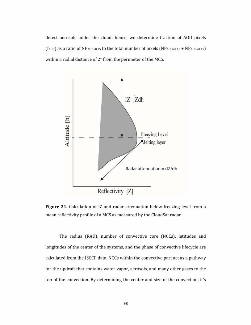
98

detect aerosols under the cloud; hence, we determine fraction of AOD pixels

(fAOD)asaratioofNPAOD>0.15tothetotalnumberofpixels(NPAOD>0.15+NPAOD<0.15)

withinaradialdistanceof2°fromtheperimeteroftheMCS.

Figure21.Calculationof IZ and radar attenuationbelow freezing level froma

meanreflectivityprofileofaMCSasmeasuredbytheCloudSatradar.

The radius (RAD), number of convective core (NCCs), latitudes and

longitudesofthecenterofthesystems,andthephaseofconvectivelifecycleare

calculatedfromtheISCCPdata.NCCswithintheconvectivepartactasapathway

fortheupdraftthatcontainswatervapor,aerosols,andmanyothergasestothe

topoftheconvection.Bydeterminingthecenterandsizeoftheconvection, it’s

99

possible to detect the position and the propagation of the cloud every three

hours.ThelifecycleofaMCSiscalculatedfromthearealtimerateofexpansion

ratio:

AE (1)

whereAistheareaoftheconvectivesystemandVisthehorizontalwindvector

[Machadoetal., 1998]. Largerpositive values ofAE (AE>0.1) are associated

with the growing stage of the convective life cycle, whereas larger negative

values (AE < –0.1) are associated with the decaying stage. Values of AE

associated with the mature MCSs are close to 0 (i.e., –0.1 ≤ AE ≤ 0.1)

[Chakrabortyetal.,2015;Machadoetal.,1998].

From the reflectivity data, we first calculate the mean reflectivity (Z)

profileforeachoftheco‐locatedMCSsandcalculateIZ(Figure21).Thelevelof

maximumreflectivitydenotesthefreezing levelor themelting layerduetothe

meltinghydrometeors[Matrosov,2009a;b;Matrosovetal.,2007].Weintegrate

themean reflectivityprofile (IZ)above the freezing level to represent the IWC

insidetheMCSs’coresabovethefreezinglevel[Matrosov,2009a]:

Zdh (2)

whereh is theheight inkm. IZ typically represents the IWCcomprisingof the

larger ice particles observed by CloudSat inside the dense core regions of the

MCSswhereIWCisoftengreaterthan400mg/m3asseenfromthe2b‐CWC‐RO

datasetfromCloudSat.Ontheotherhand,IWC216typicallyrepresentstheanvil

ofthecloudandismeasuredbytheAURAMLSsatellite.Theiceparticlesinside

100

theanvilaresmallerinsizeandIWCisalsoless(meanIWC216ofalltheMCSswe

usedis~20mg/m3).

MERRAdatasetsuccessfullydetectscloudsalongthetrackoftheA‐Train

datasets [Chakrabortyetal.,2015].TocalculateRH,weusecloud freeregions

surroundingtheMCSswithinarangeof±2° fromtheperimeterofthecloudat

850hPa(RH850)and500hPa(RH500)levels,representingthelowerandmiddle

tropospherichumidity,respectively.Thesetwoparametersareselectedbecause

they influence the humidity of the cloud base and lateral entrainment into

convection.Weusethe locationof thecenter, radius,andthetimingasperthe

ISCCPdata set since both ISCCPandMERRAdata sets are reported at every 3

hours.WealsousedthewinddatatocalculatetheVWS:

(3)

where∂uisthechangeinzonalwindspeed.ThedeeplevelVWSassociatedwith

eachMCS is calculatedas thedifferencebetween themeanwindspeedsof the

layers 925‐850 hPa and 250‐200 hPa divided by the difference between the

meangeopotentialheights(∂z)oftherespectivelayers[Petersenetal.,2006]to

represent the deep tropospheric wind shear. We have also evaluated the

influence of the lower tropospheric wind shear, defined by the mean wind

differencebetween950‐900hPaand750‐700hPa,but its correlationwith the

variance of theMCS properties appear to be small. Thus,we do not show the

analysisrelatedtothelowertroposphericwindsheareffects.TocalculateCAPE,

weusethetemperatureandthespecifichumiditydatasetsofMERRAassociated

with theMCSs.We compute CAPE between the level of free convection to the

101

levelofnobuoyancy.WeusethemeanvaluesofCAPEofallthegridcellsunder

theMCSs.Finally,meanRRundereachMCSiscalculatedfromtheTRMM2A25

data set. Mean LH profile is calculated from the TRMM 2B31 data set by

averagingtheLHvaluesundertheMCSsat13layers.

4.2.3 StatisticalmethodsIn addition to estimating the rate of changes of RR associated with

aerosolsforconstantrangesofRHandVWSvalues,wealsousemultiplelinear

regression method to infer the relative influence of aerosols and other

meteorological parameters on IZ, IWC216, and RR. In this method, dependent

variable is statistically modeled as a linear combination of independent

variables:

y β0 ∑ (4)

whereβ0istheinterceptandβj,j€[1,p]isthecoefficientassociatedwiththejthof

ppredictors.Theyisthedependentvariable,whichistheRR(orIZandIWC216)

associatedwithlargehydrometeors.Itisobtainedbyaveragingtheprecipitation

rateofallthepixelsundereachcloud.TheindependentvariablesaretheCAPE,

RH850,RH500,VWS,andfAOD.

In this paper,weuse traditionalmethods formultiple linear regression

thatselectsthecoefficientsinordertominimizetheresidualsumofsquares:

∑ 0 ∑ (5)

This approach is suitable for investigating the influence of aerosols on MCSs

since IWC and RR of the MCSs are also influenced by many other predictors

102

(meteorologicalparameters)thatarealsotightlycorrelatedwitheachotherand

influence aerosols’ distribution. In this method, the coefficients for most

significantly related predictors may be large, but with opposite signs to

compensateeachother.Themultiplelinearmodelwouldcompensatethevalues

ofthecoefficientsinsuchawaythattheydon’trepeatorreplicatetheinfluences

ofoneparameter.Themethodofcollocatingcontainsmanypotentialsourcesof

random errors. One of such is the measurement uncertainty due to the

differencesinthepartoftheMCSsthesatellitesobserve.Forexample,aCloudSat

oraTRMMswathcanpassthroughthecenteraswellasthroughtheedgeofthe

cloud. To counteract this problem, we have aggregated the entire MCSs into

differentbins.Binsareautomaticallychosenatanincrementof5samplesforthe

dependent and independent parameters. Then, multiple liner regression

generatesalinearequationforeachbin‐sizebasedonequation4.Eachequation

is also associated errors due to the linearity assumption of themethod as per

equation5.Amongallthoseequations,wechooseonewiththeminimumerror

andcalculatetheexplainedvariancesbyeachvariableintheequation.

4.3 Results

Weevaluatetherelativeinfluenceofdifferentmeteorologicalparameters

andfAODonRRthatisderivedfromTRMM2A25datasets.Figure22showsthe

rateofchangeofMCSs’RRassociatedwithonestandarddeviation(1σ)change

inCAPE,RH850(lowertropospherichumidity),RH500(ambienthumidityaround

~5.5 km altitude), fAOD, and the deep tropospheric vertical wind shear (VWS),

respectively,whenotherparametershavesimilarvalues.Ourresultsshowthat

103

with an increase in CAPE by 1σ, RR either increases at the rate up to ~0.32

mm/hunder lowVWSandhigh fAOD (Figure22a),ordecreasesat the rateof ‐

0.16mm/hunderhighVWSand low fAODvalues.RRalso increasesata rateof

0.1‐0.3mm/hwith1σ increase inRH850 (Figure22b) and at a rate of0.06‐0.3

mm/hwith1σofincreaseofRH500underlowerfAODcondition(Figure22c).RR

either decreases with fAOD under nearly saturated RH850 or VWS, or increases

withfAODunder40‐80%RH850andintermediateVWS(10‐30X10‐4S‐1)withrates

rangingbetween‐0.13to0.14mm/hdependingonmeteorologicalparameters.

ChangeofRRappeartobestrongerwiththechangesofCAPEandRHthanwith

VWSandfAOD(Figure22e,22d).

The impact of aerosols onMCSs’ rainrates depends on their interaction

withtheenvironment[DelGenioandWu,2010;R.A.Houze,2004]andmaynot

beclearlydetectablebysatellitesuntilwedivideandanalyzetheMCSsaccording

to the phases of their lifecycle. Moreover, the MCSs interact with the

environment in differentways depending on their size and structure that also

varies with different phases of lifecycle [Machado et al., 1998]. To clearly

understand the impact of aerosols on RR at different stages of lifecycle, we

compute the change in rainrates (mm/h) due to 1σ change in fAOD at three

differentphasesoflifecyclewhenotherconditionslikeRH850andVWSarefixed

toconstantvalues(Figure23).

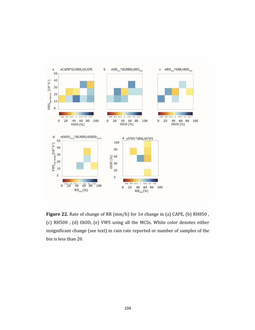
104

Figure22.RateofchangeofRR(mm/h)for1σchangein(a)CAPE,(b)RH850,

(c) RH500 , (d) fAOD, (e) VWS using all theMCSs.White color denotes either

insignificantchange(seetext)inrainratereportedornumberofsamplesofthe

binislessthan20.

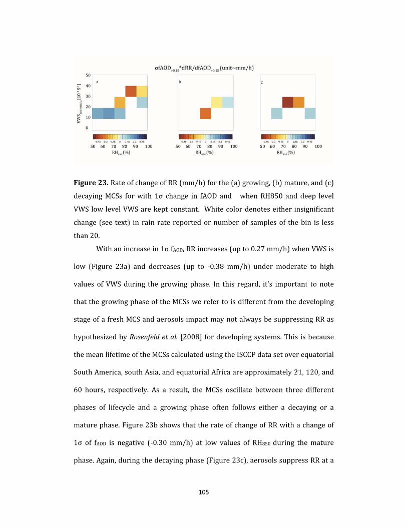
105

Figure23.RateofchangeofRR(mm/h)forthe(a)growing,(b)mature,and(c)

decayingMCSs forwith 1σ change in fAOD and whenRH850 and deep level

VWS lowlevelVWSarekeptconstant. Whitecolordenoteseitherinsignificant

change (see text) in rain rate reportedornumberof samplesof thebin is less

than20.

Withanincreasein1σfAOD,RRincreases(upto0.27mm/h)whenVWSis

low (Figure 23a) and decreases (up to ‐0.38 mm/h) under moderate to high

values of VWSduring the growingphase. In this regard, it’s important to note

thatthegrowingphaseoftheMCSswerefertoisdifferentfromthedeveloping

stageofafreshMCSandaerosolsimpactmaynotalwaysbesuppressingRRas

hypothesizedbyRosenfeldetal. [2008]fordevelopingsystems.This isbecause

themeanlifetimeoftheMCSscalculatedusingtheISCCPdatasetoverequatorial

SouthAmerica,southAsia,andequatorialAfricaareapproximately21,120,and

60 hours, respectively. As a result, the MCSs oscillate between three different

phases of lifecycle and a growing phase often follows either a decaying or a

maturephase.Figure23bshowsthattherateofchangeofRRwithachangeof

1σ of fAOD is negative (‐0.30mm/h) at low values of RH850 during themature

phase.Again,duringthedecayingphase(Figure23c),aerosolssuppressRRata

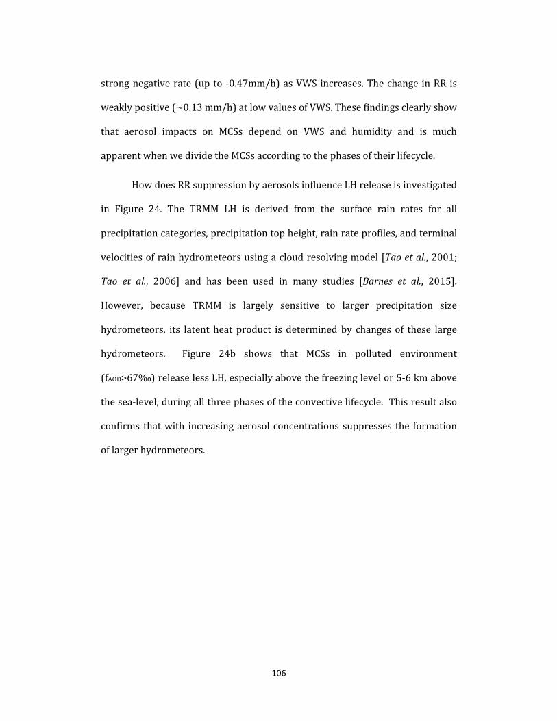
106

strongnegativerate(upto ‐0.47mm/h)asVWS increases.Thechange inRR is

weaklypositive(~0.13mm/h)atlowvaluesofVWS.Thesefindingsclearlyshow

that aerosol impacts on MCSs depend on VWS and humidity and is much

apparentwhenwedividetheMCSsaccordingtothephasesoftheirlifecycle.

HowdoesRRsuppressionbyaerosolsinfluenceLHreleaseisinvestigated

in Figure 24. The TRMM LH is derived from the surface rain rates for all

precipitationcategories,precipitationtopheight,rainrateprofiles,andterminal

velocitiesofrainhydrometeorsusingacloudresolvingmodel[Taoetal.,2001;

Tao et al., 2006] and has been used in many studies [Barnes et al., 2015].

However, because TRMM is largely sensitive to larger precipitation size

hydrometeors, its latent heat product is determined by changes of these large

hydrometeors. Figure 24b shows that MCSs in polluted environment

(fAOD>67‰)releaselessLH,especiallyabovethefreezinglevelor5‐6kmabove

thesea‐level,duringallthreephasesoftheconvectivelifecycle.Thisresultalso

confirms thatwith increasingaerosol concentrations suppresses the formation

oflargerhydrometeors.

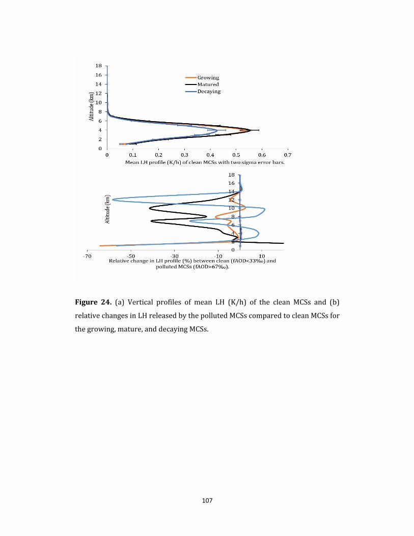
107

Figure 24. (a) Vertical profiles of mean LH (K/h) of the clean MCSs and (b)

relativechangesinLHreleasedbythepollutedMCSscomparedtocleanMCSsfor

thegrowing,mature,anddecayingMCSs.

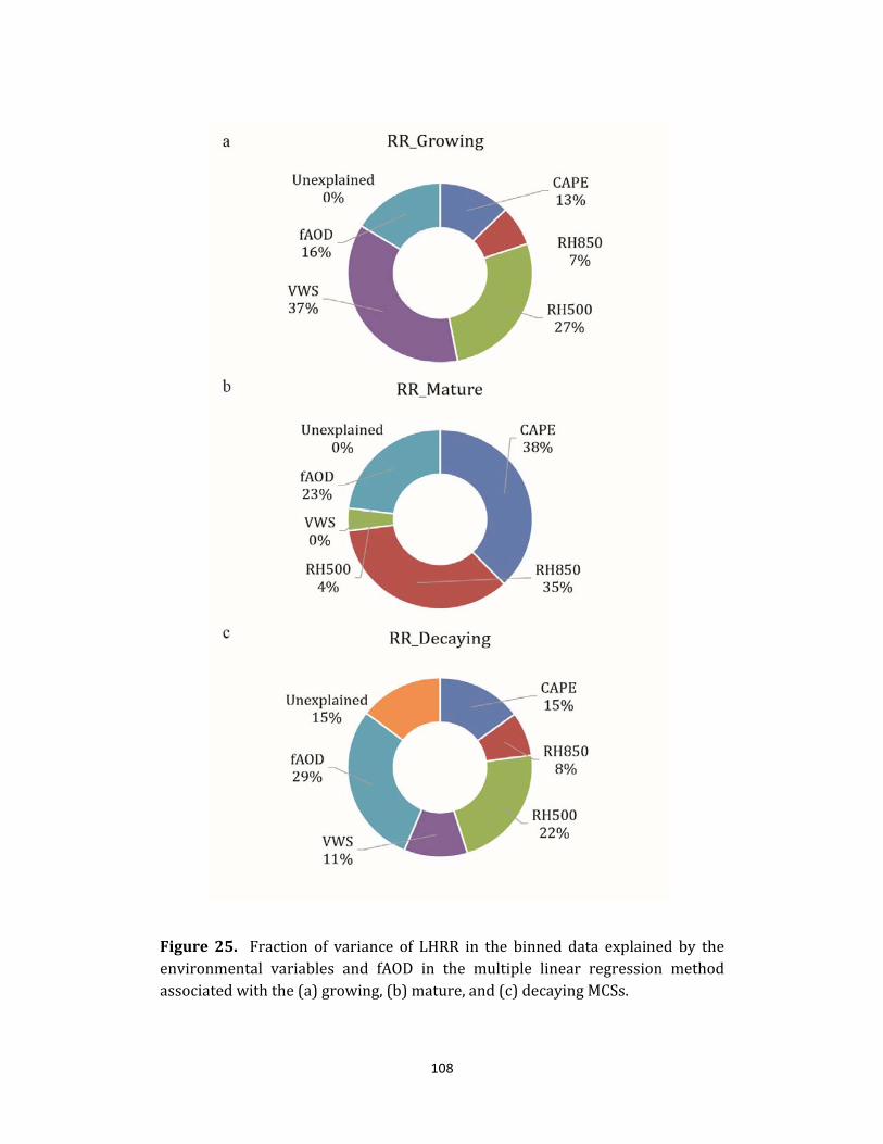
108

Figure25. Fraction of variance of LHRR in the binned data explained by theenvironmental variables and fAOD in the multiple linear regression methodassociatedwiththe(a)growing,(b)mature,and(c)decayingMCSs.

109

These results suggest that aerosols mainly suppress the RR during all

threephasesoftheconvectivelifecycle.Asaresult,aerosolsexplain16%,23%,

and 29% of the RR’s variance (Figure 25) in multivariate linear regression

during the growing, mature, and decaying phases, respectively. VWS explains

37%and11%oftheRRvariance(Figure25aand25c)duringthegrowingand

decayingphases,respectively.This isbecauseaerosolssuppress(enhances)RR

duringthosephases(Figure23aand23c)whenVWSismoderatetohigh(low).

Ontheotherhand,aerosol’simpactonRRdependsstronglyonhumidityrather

than VWS during the mature phase (Figure 23b); hence, meteorological

parametersrelatedtohumidity,suchasCAPE(derivedfromwatervapormixing

ratioandtemperature),RH850,andRH500explainthelargestfractionofvariance

(~77%)duringthematurephase(Figure23b).

RRsuppressionbyaerosolswouldleadtoanenhancementofIWCofthe

MCSs.Thus,weanalyzetheinfluencesofaerosolsontotalintegratedreflectivity

(IZ)oftheMCSsusingCloudSatdataset(Figure26a‐26c),andIWC216usingthe

AuraMicrowaveLimbSounder(MLS)dataset(Figure27a‐27c)atthreedifferent

stagesoflifecycle.Figure26showsthatanenhancementinIZoccursduringthe

growing (up to 8 dBZ), mature (up to 11dBZ), and decaying (up to 18 dBZ)

phases associated with an increase in 1σ of fAOD. These results are consistent

withthefindingsfromFigure23and24andsuggestthataerosolsincreaseMCSs’

IWC comprised of bigger‐sized ice crystals as observed by CloudSat W‐band

radarduetoadecreaseinRRasestimatedfromTRMMprecipitationradar(13.8

GHz;sensitivetolargehydrometeors).SinceaerosolsenhanceRRatlowvalues

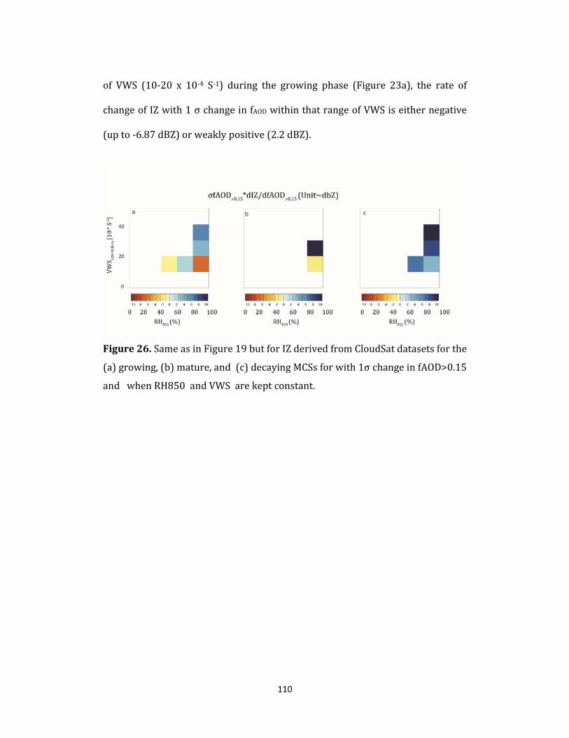
110

of VWS (10‐20 x 10‐4 S‐1) during the growing phase (Figure 23a), the rate of

changeofIZwith1σchangeinfAODwithinthatrangeofVWSiseithernegative

(upto‐6.87dBZ)orweaklypositive(2.2dBZ).

Figure26.SameasinFigure19butforIZderivedfromCloudSatdatasetsforthe

(a)growing,(b)mature,and(c)decayingMCSsforwith1σchangeinfAOD>0.15

andwhenRH850andVWSarekeptconstant.

111

Figure27.SameasinFigure19butforIWC216(mg/m3)derivedfromAuraMLS

datasets for growing, mature, and decaying MCSs for with 1σ change in

fAOD>0.15andwhenRH850anddeeplevelVWSarekeptconstant.

IWCcomprisingofthesmallersizeiceparticlesinsideanvilsoftheMCSs

alsoincrease.Duringthegrowingphase(Figure27a),IWC216increasesupto0.75

mg/m3duetoanincreasein1σoffAODwhentheVWSismoderatetohigh.When

aerosol concentration increases, anvil IWC increases by more than 1mg/m3

during the mature phase and up to 0.82 mg/m3 during the decaying phase

(Figure27c).LikeIZ(Figure26a),IWC216alsodecreaseswithincreasingaerosol

concentrationsatlowvaluesofVWS(Figure27a)duringthegrowingphase.This

is consistentwithan increaseofRRwith fAODunder thesimilarmeteorological

conditions(Figure23a).

We also look at the variances of IZ and IWC216 explained by different

meteorological parameters (Figure 26). CAPE is the dominant parameter that

explains most of IZ’s variance during all three phases of MCS’s lifecycle. VWS

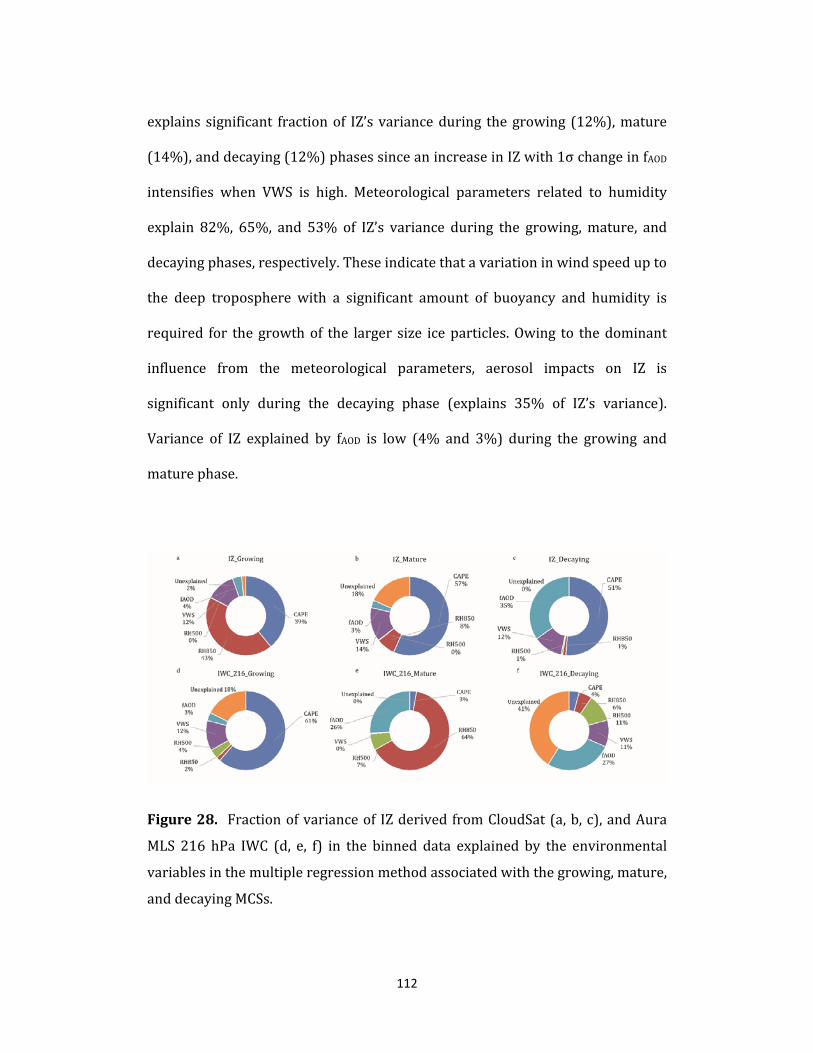
112

explains significant fractionof IZ’svarianceduring thegrowing (12%),mature

(14%),anddecaying(12%)phasessinceanincreaseinIZwith1σchangeinfAOD

intensifies when VWS is high. Meteorological parameters related to humidity

explain 82%, 65%, and 53% of IZ’s variance during the growing,mature, and

decayingphases,respectively.Theseindicatethatavariationinwindspeedupto

the deep troposphere with a significant amount of buoyancy and humidity is

required for thegrowthof the larger size iceparticles.Owing to thedominant

influence from the meteorological parameters, aerosol impacts on IZ is

significant only during the decaying phase (explains 35% of IZ’s variance).

Variance of IZ explained by fAOD is low (4% and 3%) during the growing and

maturephase.

Figure28. Fractionofvarianceof IZderivedfromCloudSat(a,b,c),andAura

MLS 216 hPa IWC (d, e, f) in the binned data explained by the environmental

variablesinthemultipleregressionmethodassociatedwiththegrowing,mature,

anddecayingMCSs.

113

Meteorological parameters also dominate the fraction of variance of

IWC216explainedduring thegrowing(67%)andmature(74%)phases,butnot

during the decaying (21%) phase. fAOD explains 26% and 27% of IWC216’s

variance during the mature (δIWC216>1 mg/m3, Figure 27b) and decaying

(δIWC216 ~0.82 mg/m3, Figure 27c) phases. Variance of IWC216 as well as IZ

explained by fAOD during the growing phases is low (~3 and 4%, respectively,

Figures28aand28d)becauseofboththepositive(enhancement)andnegative

(reduction) impacts of aerosols on IWC216 (Figure 23a) and IZ (Figure 22a)

duringthatphase.

IZandIWC216derivedfromCloudSatandAuraMLS(Figures26,27,and

28)andtheRR(Figures22,23,and25)andLH(Figure24)derivedfromTRMM

data set are consistent with each other and show that aerosols suppress the

MCSs’ precipitation and enhance IWC inside the dense convective as well as

stratiformregions.

4.4 Conclusion

This is the first study using a suite of different andmulti‐year satellite

data sets to estimate the relative influence of the aerosols and other

meteorological parameters on the strength and precipitation of theMCSs. Our

studyshowsthatthedifferentsatellitestakingmeasurementsofdifferentMCSs

are consistent with each other. TRMM 2A25 data set shows that aerosols

suppressRRduringallthreephasesofconvectivelifecycle,especiallyunderthe

influence of high VWS during the growing and decaying phases and in dry

conditionsduringthematurephase.Duringthegrowingphase, fAODsuppresses

114

RRunderhighVWS(‐0.38mm/h).DuringthematurephaseRRissuppressedby

‐0.30mm/hunderdryenvironmental conditions,whereasduring thedecaying

phaseRRissuppressedby‐0.47mm/h,againundertheinfluenceofhighVWS.

As a result, aerosols explain 16%, 23%, and 29% of RR’s variance inmultiple

linearregressionduringthegrowing,mature,anddecayingphases,respectively.

VWSexplains37%and11%ofRR’svarianceduring thegrowinganddecaying

phases only because if its influence on aerosols impacts on RR during those

phases.SuppressionofRRbyincreasingaerosolconcentrationleadstoareduced

LHrelease(Figure24).ThesuppressionofRRbyaerosolsisduetothefactthat

theyinvigoratetheMCSsbyenhancingIWCoftheMCSs.Aerosolsincreaseboth

IZandIWC216duringthegrowing,mature,anddecayphases(Figure26and27).

TheimpactofaerosolsonIZisintensifiedwhenVWSincreasesfrommoderateto

highvaluesduringallthreephasesofconvectivelifecycle.IncreaseinanvilIWC

withincreasingaerosolconcentrationsalsooccursathighvaluesofVWSduring

thegrowingphase (Figure27a) andVWSexplains12%of its variance (Figure

28d).Hence,ouranalysesusingdifferentsatellitedatasetsareconsistentwith

eachotherandshowthataerosolsintensifytheMCSsbyenhancingtheIWCand

reducingtherainratesduringallthreephasesoflifecycle.

Duringthegrowingphase,aerosolssuppress(enhance)RRandintensify

(reduce)bothIZandIWC216undermoderatetohigh(low)valuesofVWS.This

suggests that VWS plays an important role in convective development and

precipitation during the growing phase. This could be because of the fact that

VWS plays important roles in organizing the storms, location of updraft and

115

downdraft regions, and slantwise accentof themoist air [KingsmillandHouze,

1999;Moncrieff,1978;WeismanandRotunno,2004]andtheMCSsarerootedto

theboundarylayerduringthatphase[R.A.Houze,2004].Detailedanalysisusing

cloudmicrophysics is required to explore this interdependence between VWS

and aerosol concentrations during that phase. However, other meteorological

parameters such asCAPE, lower tropospheric humidity, and ambienthumidity

enhance RR. CAPE, RH850, and RH500 increases RR up to 0.32, 0.3, and 0.2

mm/h,respectivelyandtheyexplainthelargestfractionofRR’svariance(47%,

77%,and45%,respectively)whenweconsideralltheMCSs.InfluenceofCAPE

and lower tropospherichumidityonRRhasbeendocumented inmanystudies

[Robert A. Houze, 1993; R. A. Houze, 2004;Mapes, 1993] and Langhans et al.

[2015] in a recent study showed that entrainment humidity contributes up to

one‐thirdtoone‐halfofthesurfacerainfall.

OurstudyusesobservationsfromtheA‐Trainbasedmeasurementstaken

approximatelyat1:30amand1:30pmlocaltime,whereasthepeakstrengthare

achieved by the MCSs during the evening time. Further study using cloud

microphysics at three different phases of convective lifecycle is needed to

understandaerosolimpactsontheMCSs.

116

Chapter5

GeneralConclusions

The findingspresented in thisdissertationarebasedon theanalysesof

multi‐year satellite datasets to resolve the relationships between UT ALs

surrounding the MCSs and MCS morphology at three different phases of

convective lifecycle and to provide a large‐scale statistical assessment of the

relativeinfluenceofaerosolsandmeteorologicalconditions(CAPE,RHandVWS)

on the rain rates, ice water content, and longevity of the MCSs. To our

knowledge, this is the first satellite‐based global tropical continental‐scale

assessment of aerosol‐MCS relationships using collocated MCS samples from

different satellite observations. These include geostationary ISCCP convective

tracking, the A‐train constellation, and TRMM, along with MERRA reanalysis

products.ThisdissertationusesmultipledatasetsfromA‐Trainmeasurementsto

obtain aerosol information from CALIPSO, Aqua MODIS, and OMI and cloud

informationfromCloudSatandAuraMLSdatasets.Informationaboutrainrates

andlatentheatareobtainedfromTRMMmeasurements.

This dissertation consists of four chapters. Chapter 1 introduces the

subjectmatter and discusses the importance of aerosols in the context of the

MCSs and global climate. Chapter 2 focuses on the estimation of the extent of

uppertroposphericaerosollayers(UTALs)surroundingtheMCSsandexplores

the relationships between the extent of such ALs and the morphology of the

MCSslocatedoverdifferenttropicalcontinentalregions.Suchrelationshipsand

thevariationofUTALsarederivedat threedifferentphasesof the convective

117

lifecycle.Ouranalysis isbasedonsatellitedatacollectedoverequatorialAfrica,

SouthAsia,andtheAmazonbasinbetweenJune2006andJune2008.Weidentify

substantial variations in the relationships between convective properties and

aerosol transport by region and stage of convective development. The most

extensiveUTALsoverequatorialAfricaareassociatedwithmatureMCSs,while

themostextensiveUTALsoverSouthAsiaandtheAmazonareassociatedwith

growing MCSs. Convective aerosol transport over the Amazon is weaker than

thatobservedovertheothertworegionsdespitesimilartransportfrequencies,

likely due to the smaller sizes and shorter mean lifetimes of MCSs over the

Amazon.

Variations in UT ALs in the vicinity of tropical MCSs are primarily

explained by variations in the horizontal sizes of the associatedMCSs and are

largely unrelated to aerosol loading in the lower troposphere. In addition, we

identifypotentiallyimportantrelationshipswiththenumberofconvectivecores,

vertical wind shear, and convective fraction during the growing and mature

stages of MCS development. Relationships between convective properties and

aerosol transport are relatively weak during the decaying stage of convective

development.

Our analysis indicates that VWSmay play an important role in aerosol

transport during the growing stage. The VWS coefficient appears to act as a

surrogate forregionalvariabilitywhenall regionsareconsidered together,but

ALextentoverSouthAsiaincreasessignificantlywithincreasingVWS(R=0.30,

p = 0.03). A positive relationship between VWS and aerosol transport is

118

physically plausible, given the close relationship between convective and

boundarylayerpropertiesduringthegrowingstageandthepotentialforVWSto

enhance convective aerosol transport by establishing separate regions for

updrafts and downdrafts. Our statistical model results further indicate that

mature systems with similar sizes will typically produce more extensive ALs

when the CF is larger. This positive dependence on CF is only observed for

maturesystems.Bycontrast,theextentofALsassociatedwithdecayingsystems

isnegativelycorrelatedwithaerosolopticaldepth(AOD).Ourresultsprovidean

interpretive framework for devising and evaluating numerical model

experimentsthatexaminerelationshipsbetweenconvectivepropertiesandALs

intheuppertroposphere.

Chapter3 focuseson the relative influenceofmeteorological conditions

andaerosolson the lifetimeof theMCSs.Using collocatedmeasurements from

geostationaryandpolar‐orbitalsatellitesovertropicalSouthAmerica,equatorial

Africa, and South Asia, we provide a large‐scale statistical assessment of the

relativeinfluenceofaerosolsandmeteorologicalconditionsonthelifetimeofthe

MCSs.SinceweuseTRMM,whichorbitstheEarthonadifferenttrackandata

different time compared to the A‐Train satellites, we are able to extend our

collocation period from January 2003 to June 2008 in order to have a larger

number of samples. Our results show that globally, over tropical continental

regions, MCSs’ lifetime increases by 3‐24 hours with ambient aerosol optical

depth (AOD)only underhigh relativehumidity (RH) in the lower troposphere

andmoderateverticalwindshear(VWS)inthedeeptroposphere.However,the

119

influence of aerosols is not as strong as that of convective available potential

energy(12‐36hours),RH(6‐30hours)anddeeptroposphericVWS(3‐30hours),

which explain 18‐22%, 44‐62%, and 8‐18% of the total variance of MCSs’

lifetime, respectively. AOD explains up to 19% of the total variance of MCSs’

lifetimemainly during the decaying phase. This result is physically consistent

with thevariationof theMCSs’ icewater content inside their convective cores

andanvils,whichpeakduringthedecayingphase(35%and27%,respectively).

TheeffectofaerosolsonMCSs’ lifetimevariesbetweencontinents.AOD

appears to explain up to 20%‐22% of the total variance in MCS lifetime over

equatorialSouthAmericacomparedto8%overequatorialAfrica.Aerosolsover

the IndianOcean can explain 14% of the total variance inMCSs’ lifetime over

SouthAsiabecausemostMCSsformanddevelopovertheocean.UsingAOD>0.3

as a threshold did not produce any observable difference in terms of aerosol

impactsonMCSs.WealsoobservethattheimpactsfromthelowlevelVWSare

poorlycorrelatedwithMCSlifetimeascomparedtodeeplevelVWS.

To our knowledge, this is the first satellite based global tropical

continental scale assessment of the relative roles of the meteorological

conditionsandaerosolsusing largesamplesof theMCSs.Thisstudyprovidesa

global tropical assessment on the relative influences of aerosols and

meteorologicalconditionsonMCCs’lifetimeandthemutualdependenceofthese

influences.Italsoshowshowaerosolsinfluenceonthecloudiceandlifetimeof

theMCSs varywithin their lifecycle and between different tropical continents

ranging from humid equatorial South America during wet season and big

120

monsoonalsystemsoverSouthAsiatorelativelydryequatorialAfricawithhigh

aerosol loading. In doing so, this work has also advanced our capability to

evaluatewhetherornotaerosols could increase convective lifetimeon climate

scaleandwhatarethefavorablemeteorologicalconditionsforaerosoltoaffect

thelifetimeoftheMCSs.

These regional differences in the aerosol impact appear to be linked to

differentmeteorological conditions, but the underlying physical processes and

influences of varying aerosol types require further investigation in the future.

Moreover,weareunabletoobservethemicrophysicalchangesassociatedwith

MCS convections at different phases of convective lifetime and over different

geographic regions. To understand the influence from different types of

aerosols,aircraftobservationsandground‐basedmeasurementscanbeused in

thefuture.

Thefocusofchapter4istoestimatetherelativeinfluenceofaerosolsand

other meteorological conditions on rain rates (RR), cloud ice water content

(IWC), and latent heat (LH) profiles through the life cycle of large mesoscale

convective systems (MCSs) over the tropical South America, Africa and South

Asia for the period of January 2003‐ June2008 using a suite of co‐located

geostationary and polar orbital satellite measurements. Under similar lower

tropospheric humidity (RH850) and vertical wind shear (VWS) conditions, an

increase in aerosol concentrations tends to suppress RR and LH, but intensify

cloudicebothintheconvectivecoresandanvilsthroughconvectivelifecycle.In

particular,an increaseofaerosolconcentrationsbyonestandarddeviationcan

121

suppressRRduringtheentireconvectivelifecycle,especiallyduringthegrowing

phaseanddecayphases,attherateof‐0.38mm/hand‐0.47mm/h,respectively,

whenVWSishigh,andduringthematurephasewhenthehumidityislowatthe

rate of ‐0.30 mm/h. Consequently, LH released by the MCSs decreases also

because it is dominated by the observation of RR by TRMM. Aerosols explain

16%,23%,and29%ofRR’svarianceduringthegrowing,matureanddecaying

phases, respectively, over the global tropical continents, as estimated by a

multiplelinearregressionmethod.

By comparison, increasing convective available potential energy (CAPE)

and humidity (RH850 or lower tropospheric humidity and RH500 or ambient

humidity) explain 47%, 77%, and 45% of the total RR’s variance during the

growing, mature, and decaying phases, respectively. The rate of enhance RR

with CAPE, RH850 and RH500 is up to 0.32 mm/h, 0.3 mm/h, and 0.3 mm/h,

respectively. Different studies have documented the influence of CAPE and

lower tropospheric humidity onRR [RobertA.Houze, 1993;R.A.Houze, 2004;

Mapes,1993].Langhansetal.[2015]inarecentstudyshowedthatentrainment

humidity contributes up to one‐third to one‐half of the surface rainfall. Our

findings are consistentwith the previous findings that stronger buoyancy and

higher amount of moisture would enhance the RR, whereas aerosols would

suppressRRandintensifytheMCSsbyenhancingtheirIWC.VWSexplains37%

and11%ofRR’svarianceduringthegrowinganddecayingphasesonlybecause

if its influence on aerosols impacts on RR during those phases. Strong VWS

contributes to aerosol impacts by suppressing RR and enhancing IWC. On the

122

otherhand,IWCinsidethecoreandanvilregionsoftheMCSsdecreasesandRR

increaseswithincreasingaerosolsconcentrationswhenVWSislow.Thismight

be due to the fact that VWS plays an important role in organizing relative

position of the updraft and downdraft regions, tilting of the systems, and

slantwise ascent of themoisture inside theMCSs [Kingsmill andHouze, 1999;

Moncrieff, 1978;Weisman and Rotunno, 2004], especially during the growing

phasewhenthestormsarerootedtotheirboundarylayer[R.A.Houze,2004].

IWCoftheMCSsincreasesduringallthreephasesofconvectivelifecycle,

as expected from the increase of smaller cloud particle with aerosols and

reducedRR.Withincreasingaerosolconcentrations,totalintegratedreflectivity

of the largercloud iceparticles,asdetectedbyCloudSat, increasesup to8,11,

and 18 dBZ in the convective core regions during the growing, mature and

decayingphases,respectively.TheIWCinsideanvils,comprisedofsmaller‐sized

ice particles as detected by Aura MLS, also increases by 0.72, 1.41, and 0.82

mg/m3duringthegrowing,mature,anddecayingphases,respectively.

Using satellite data sets over global tropical continents, this study

provides an assessment of the relative influences of the meteorological

conditions and aerosols on MCS rain rate and IWC. It also show how aerosol

impacts on MCS rain rate and IWC vary at different phases of the convective

lifetimeandhowmeteorologicalparametersinfluencethat.Hence,thisworkhas

also advanced our capability to evaluate whether or not aerosols could

invigoratetheMCSs.

123

IuseobservationsfromtheA‐Trainbasedmeasurementsthataretaken

approximatelyat1:30amand1:30pmlocaltime,whereasthepeakstrengthare

achieved by the MCSs during the evening time. Further study using cloud

microphysics at three different phases of convective lifecycle is needed to

understand aerosol impacts on theMCSs. Use of ground‐basedmeasurements

couldprovidedetailedexplanationofthesefindingsandcanalsoinvestigatethe

sameatthepeakconvectivestrength.

Thisdissertation focusedonaerosol‐MCSrelationshipsover the tropical

continents.Sofar,wehaveinvestigatedtheinfluenceoffAOD,RH,CAPE,andVWS

ontheMCSs.However,theMCSsovertheextra‐tropicsarefrontalandbaroclinic

in nature; hence, temperature gradient might be another important

meteorological parameter that can have a significant influence on the MCSs.

Understanding the transport of aerosols along the frontal boundary of extra‐

topicalcloudsandtheinfluenceofaerosolsandothermeteorologicalparameters

onMCSswill be the focus of futurework. In addition, I intend to focus on the

relative influences of those meteorological parameters and aerosols on the

mechanismof self‐aggregationof convections [WingandEmanuel, 2014]using

both satellite and ground‐based measurements of the Department of Energy

AtmosphericRadiationMeasurement(ARM)datasets.

124

References

Ackerman,A.S.,O.B.Toon,D.E.Stevens,A.J.Heymsfield,V.Ramanathan,andE.J.Welton (2000), Reduction of tropical cloudiness by soot, Science,288(5468),1042‐1047.Albrecht,B.A.(1989),Aerosols,CloudMicrophysics,andFractionalCloudiness,Science,245(4923),1227‐1230.Altaratz, O., I. Koren, L. A. Remer, and E. Hirsch (2014), Review: Cloudinvigoration by aerosols‐Coupling betweenmicrophysics and dynamics,AtmosRes,140,38‐60.Andreae,M.O.,D.Rosenfeld,P.Artaxo,A.A.Costa,G.P.Frank,K.M.Longo,andM. A. F. Silva‐Dias (2004), Smoking rain clouds over the Amazon, Science,303(5662),1337‐1342.Barnes, H. C., M. D. Zuluaga, and R. A. Houze (2015), Latent heatingcharacteristics of theMJO computed from TRMMObservations, JGeophysRes‐Atmos,120(4),1322‐1334.Bell, T. L., D. Rosenfeld, K. M. Kim, J. M. Yoo, M. I. Lee, and M. Hahnenberger(2008), Midweek increase in US summer rain and storm heights suggests airpollutioninvigoratesrainstorms,JGeophysRes‐Atmos,113(D2).Bhowmik, S. K. R., S. Sen Roy, and P. K. Kundu (2008), Analysis of large‐scaleconditions associated with convection over the Indian monsoon region, Int JClimatol,28(6),797‐821.Bister,M., andM.Kulmala (2011),Anthropogenicaerosolsmayhave increaseduppertropospherichumidityinthe20thcentury,AtmosChemPhys,11(9),4577‐4586.Chakraborty,S.,R.Fu,J.S.Wright,andS.T.Massie(2015),Relationshipsbetweenconvectivestructureandtransportofaerosolstotheuppertropospherededucedfromsatelliteobservations,JGeophysRes‐Atmos,120(13),6515‐6536.Charlson,R.J.,S.E.Schwartz,J.M.Hales,R.D.Cess,J.A.Coakley,J.E.Hansen,andD. J. Hofmann (1992), Climate Forcing by Anthropogenic Aerosols, Science,255(5043),423‐430.Chu,D.A.,Y.J.Kaufman,L.A.Remer,D.Tanre,andM.J.Jeong(2003),Multi‐yearMODIS observation of global aerosols from EOS Terra/Aqua satellites:Validation,variability,andapplication,IntGeosciRemoteSe,863‐865.Chu,D.A.,Y.J.Kaufman,C.Ichoku,L.A.Remer,D.Tanre,andB.N.Holben(2002),ValidationofMODISaerosolopticaldepthretrievalover land,GeophysResLett,29(12).Chung,C.E.,andV.Ramanathan(2004),Aerosol loadingovertheIndianOceananditspossibleimpactonregionalclimate,IndianJMarSci,33(1),40‐55.Chylek,P.,M.K.Dubey,U.Lohmann,V.Ramanathan,Y. J.Kaufman,G.Lesins, J.Hudson,G.Altmann,andS.Olsen(2006),AerosolindirecteffectovertheIndianOcean,GeophysResLett,33(6).Cotton,W.R.,andR.A.Anthes(1989),Stormandclouddynamics,xii,883p.pp.,AcademicPress,SanDiego.

125

Cotton,W.R.,G.D.Alexander,R.Hertenstein,R.L.Walko,R.L.McAnelly,andM.Nicholls(1995),Cloudventing‐Areviewandsomenewglobalannualestimates,Earth‐SciRev,39(3‐4),169‐206.Crutzen,P.J.,andM.O.Andreae(1990),BiomassBurningintheTropics‐ImpactonAtmosphericChemistryandBiogeochemicalCycles,Science,250(4988),1669‐1678.deBoer,G.,T.Hashino,andG.J.Tripoli(2010),Icenucleationthroughimmersionfreezing in mixed‐phase stratiform clouds: Theory and numerical simulations,AtmosRes,96(2‐3),315‐324.DelGenio,A.D.,andJ.B.Wu(2010),TheRoleofEntrainmentintheDiurnalCycleofContinentalConvection,JClimate,23(10),2722‐2738.Di Pierro, M., L. Jaegle, and T. L. Anderson (2011), Satellite observations ofaerosol transport fromEastAsia to theArctic: three case studies,AtmosChemPhys,11(5),2225‐2243.Ekman, A.M. L., C.Wang, J. Strom, andR. Krejci (2006), Explicit simulation ofaerosolphysicsinacloud‐resolvingmodel:Aerosoltransportandprocessinginthefreetroposphere,JAtmosSci,63(2),682‐696.Ervens, B., G. Feingold, G. J. Frost, and S. M. Kreidenweis (2004), A modelingstudy of aqueous production of dicarboxylic acids: 1. Chemical pathways andspeciatedorganicmassproduction,JGeophysRes‐Atmos,109(D15).Fan, J.W., R. Y. Zhang, G. H. Li, andW. K. Tao (2007), Effects of aerosols andrelativehumidityoncumulusclouds,JGeophysRes‐Atmos,112(D14).Fan, J.W.,L.R.Leung,D.Rosenfeld,Q.Chen,Z.Q.Li, J.Q.Zhang,andH.R.Yan(2013), Microphysical effects determine macrophysical response for aerosolimpactsondeepconvectiveclouds,PNatlAcadSciUSA,110(48),E4581‐E4590.Fan,J.W.,T.L.Yuan,J.M.Comstock,S.Ghan,A.Khain,L.R.Leung,Z.Q.Li,V. J.Martins, andM. Ovchinnikov (2009), Dominant role by vertical wind shear inregulatingaerosoleffectsondeepconvectiveclouds,JGeophysRes‐Atmos,114.Fan, S. M., L. W. Horowitz, H. Levy, and W. J. Moxim (2004), Impact of airpollutiononwetdepositionofmineraldustaerosols,GeophysResLett,31(2).Froyd,K.D.,D.M.Murphy,T.J.Sanford,D.S.Thomson,J.C.Wilson,L.Pfister,andL. Lait (2009), Aerosol composition of the tropical upper troposphere, AtmosChemPhys,9(13),4363‐4385.Fu,R.,Y.L.Hu,J.S.Wright,J.H.Jiang,R.E.Dickinson,M.X.Chen,M.Filipiak,W.G.Read,J.W.Waters,andD.L.Wu(2006),ShortcircuitofwatervaporandpollutedairtotheglobalstratospherebyconvectivetransportovertheTibetanPlateau,PNatlAcadSciUSA,103(15),5664‐5669.Glaccum, R. A., and J.M. Prospero (1980), Saharan Aerosols over the TropicalNorth‐Atlantic‐Mineralogy,MarGeol,37(3‐4),295‐321.Gunn,R.,andB.B.Phillips(1957),AnExperimentalInvestigationoftheEffectofAirPollutionontheInitiationofRain,JMeteorol,14(3),272‐280.Harrison, S. J. (1992),FundamentalsofWeatherandClimate ‐Mcilveen,R,ScotGeogrMag,108(2),133‐133.Heald, C. L., et al. (2011), Exploring the vertical profile of atmospheric organicaerosol:comparing17aircraftfieldcampaignswithaglobalmodel,AtmosChemPhys,11(24),12673‐12696.

126

Heese, B., and M. Wiegner (2008), Vertical aerosol profiles from Ramanpolarization lidar observations during the dry season AMMA field campaign, JGeophysRes‐Atmos,113(D17).Heymsfield, A. J., C. Schmitt, and A. Bansemer (2013), Ice Cloud Particle SizeDistributions and Pressure‐Dependent Terminal Velocities from In SituObservations at Temperatures from 0 degrees to‐86 degrees C, J Atmos Sci,70(12),4123‐4154.Hodson, M. C. (1986), Raindrop Size Distribution, J Clim ApplMeteorol, 25(7),1070‐1074.Hofmann, D. J. (1990), Increase in the Stratospheric Background Sulfuric‐AcidAerosolMassinthePast10Years,Science,248(4958),996‐1000.Hoose,C.,U.Lohmann,R.Erdin,andI.Tegen(2008),Theglobalinfluenceofdustmineralogical composition on heterogeneous ice nucleation in mixed‐phaseclouds,EnvironResLett,3(2).Houze,R.A.(1993),Clouddynamics,xxix,573p.pp.,AcademicPress,SanDiego,Calif.Houze,R.A.(2004),Mesoscaleconvectivesystems,RevGeophys,42(4).Houze, R. A., K. L. Rasmussen, M. D. Zuluaga, and S. R. Brodzik (2015), Thevariablenatureofconvectioninthetropicsandsubtropics:Alegacyof16yearsof the Tropical Rainfall Measuring Mission satellite, Rev Geophys, 53(3), 994‐1021.Huang,L.,R.Fu,and J.H. Jiang(2014), Impactsof fireemissionsand transportpathwaysonthe interannualvariationofCO inthetropicalupper troposphere,AtmosChemPhys,14(8),4087‐4099.Huang, L., R. Fu, J. H. Jiang, J. S. Wright, and M. Luo (2012), Geographic andseasonaldistributionsofCOtransportpathwaysandtheirroles indeterminingCOcentersintheuppertroposphere,AtmosChemPhys,12(10),4683‐4698.Huang,L., J.H. Jiang,J.L.Tackett,H.Su,andR.Fu(2013),Seasonalanddiurnalvariations of aerosol extinction profile and type distribution from CALIPSO 5‐yearobservations,JGeophysRes‐Atmos,118(10),4572‐4596.Huffman,G.J.,R.F.Adler,D.T.Bolvin,G.J.Gu,E.J.Nelkin,K.P.Bowman,Y.Hong,E. F. Stocker, and D. B. Wolff (2007), The TRMM multisatellite precipitationanalysis (TMPA): Quasi‐global, multiyear, combined‐sensor precipitationestimatesatfinescales,JHydrometeorol,8(1),38‐55.Ichoku, C., L. A. Remer, Y. J. Kaufman, R. Levy, D. A. Chu, D. Tanre, and B. N.Holben (2003), MODIS observation of aerosols and estimation of aerosolradiativeforcingoversouthernAfricaduringSAFARI2000,JGeophysRes‐Atmos,108(D13).Ito,A.,A.Ito,andH.Akimoto(2007),SeasonalandinterannualvariationsinCOandBCemissions fromopenbiomassburning inSouthernAfricaduring1998‐2005,GlobalBiogeochemCy,21(2).Jiang,H.L.,H.W.Xue,A.Teller,G.Feingold,andZ.Levin(2006),Aerosoleffectsonthelifetimeofshallowcumulus,GeophysResLett,33(14).Jiang, J. H., H. Su, S. T. Massie, P. R. Colarco, M. R. Schoeberl, and S. Platnick(2009), Aerosol‐CO relationship and aerosol effect on ice cloud particle size:Analyses from Aura Microwave Limb Sounder and Aqua Moderate ResolutionImagingSpectroradiometerobservations,JGeophysRes‐Atmos,114.

127

Jiang, J.H.,H. Su,M.R. Schoeberl, S. T.Massie, P. Colarco, S. Platnick, andN. J.Livesey (2008), Clean and polluted clouds: Relationships among pollution, iceclouds,andprecipitationinSouthAmerica,GeophysResLett,35(14).Kacenelenbogen,M.,M.A.Vaughan, J.Redemann,R.M.Hoff,R.R.Rogers,R.A.Ferrare, P. B. Russell, C. A. Hostetler, J. W. Hair, and B. N. Holben (2011), Anaccuracy assessment of the CALIOP/CALIPSO version 2/version 3 daytimeaerosolextinctionproductbasedonadetailedmulti‐sensor,multi‐platformcasestudy,AtmosChemPhys,11(8),3981‐4000.Kato,S.,etal.(2011),Improvementsoftop‐of‐atmosphereandsurfaceirradiancecomputationswith CALIPSO‐, CloudSat‐, andMODIS‐derived cloud and aerosolproperties,JGeophysRes‐Atmos,116.Kaufman,Y.J.,D.Tanre,andO.Boucher(2002),Asatelliteviewofaerosolsintheclimatesystem,Nature,419(6903),215‐223.Keil, A., and J.M.Haywood (2003), Solar radiative forcing bybiomass burningaerosolparticlesduringSAFARI2000:Acasestudybasedonmeasuredaerosolandcloudproperties,JGeophysRes‐Atmos,108(D13).Khain,A.,andA.Pokrovsky(2004),Simulationofeffectsofatmosphericaerosolsondeepturbulentconvectivecloudsusingaspectralmicrophysicsmixed‐phasecumuluscloudmodel.PartII:Sensitivitystudy,JAtmosSci,61(24),2983‐3001.Khain, A., D. Rosenfeld, and A. Pokrovsky (2005), Aerosol impact on thedynamics and microphysics of deep convective clouds, Q J Roy Meteor Soc,131(611),2639‐2663.Khain,A.,A.Pokrovsky,M.Pinsky,A.Seifert,andV.Phillips(2004),Simulationofeffects of atmospheric aerosols on deep turbulent convective clouds using aspectral microphysics mixed‐phase cumulus cloud model. Part I: Modeldescriptionandpossibleapplications,JAtmosSci,61(24),2963‐2982.Khain, A. P., N. BenMoshe, and A. Pokrovsky (2008), Factors determining theimpact of aerosols on surface precipitation from clouds: An attempt atclassification,JAtmosSci,65(6),1721‐1748.Kilroy,G.,R.K.Smith,andU.Wissmeier(2014),Tropicalconvection:theeffectsofambientverticalandhorizontalvorticity,QJRoyMeteorSoc,140(682),1756‐1770.Kingsmill,D.E.,andR.A.Houze(1999),Kinematiccharacteristicsofairflowinginto and out of precipitating convection over the west Pacific warm pool: AnairborneDopplerradarsurvey,QJRoyMeteorSoc,125(556),1165‐1207.Knippertz, P.,M. Tesche, B.Heinold,K. Kandler, C. Toledano, andM. Esselborn(2011),DustmobilizationandaerosoltransportfromWestAfricatoCapeVerde‐ameteorologicaloverviewofSAMUM‐2,TellusB,63(4),430‐447.Koffi, B., et al. (2012),Applicationof theCALIOP layerproduct to evaluate thevertical distribution of aerosols estimated by globalmodels: AeroCom phase Iresults,JGeophysRes‐Atmos,117.Koren, I., G. Feingold, and L. A. Remer (2010a), The invigoration of deepconvective clouds over the Atlantic: aerosol effect, meteorology or retrievalartifact?,AtmosChemPhys,10(18),8855‐8872.Koren, I., J.V.Martins,L.A.Remer, andH.Afargan (2008), Smoke invigorationversusinhibitionofcloudsovertheAmazon,Science,321(5891),946‐949.

128

Koren,I.,Y.J.Kaufman,D.Rosenfeld,L.A.Remer,andY.Rudich(2005),Aerosolinvigoration and restructuring of Atlantic convective clouds,Geophys Res Lett,32(14).Koren, I.,L.A.Remer,O.Altaratz, J.V.Martins,andA.Davidi (2010b),Aerosol‐induced changes of convective cloud anvils produce strong climate warming,AtmosChemPhys,10(10),5001‐5010.L'Ecuyer, T. S., and J. H. Jiang (2010), Touring the atmosphere aboard the A‐Train,PhysToday,63(7),36‐41.Lacis, A., J. Hansen, and M. Sato (1992), Climate Forcing by StratosphericAerosols,GeophysResLett,19(15),1607‐1610.Langenberg,H.(2005),Insideinformation,Nature,437(7058),468‐469.Langhans,W.,K.Yeo, andD.M.Romps (2015),Lagrangian Investigationof thePrecipitationEfficiencyofConvectiveClouds,JAtmosSci,72(3),1045‐1062.Lee, J., J. Kim, P. Yang, and N. C. Hsu (2012), Improvement of aerosol opticaldepthretrievalfromMODISspectralreflectanceovertheglobaloceanusingnewaerosolmodelsarchived fromAERONET inversiondataandtri‐axialellipsoidaldustdatabase,AtmosChemPhys,12(15),7087‐7102.Lee, S. S. (2012), Effect of Aerosol on Circulations and Precipitation in DeepConvectiveClouds,JAtmosSci,69(6),1957‐1974.Lee, S. S., W. K. Tao, and C. H. Jung (2014), Aerosol Effects on Instability,Circulations,Clouds,andPrecipitation,AdvMeteorol.Levy,R.C.,L.A.Remer,R.G.Kleidman,S.Mattoo,C.Ichoku,R.Kahn,andT.F.Eck(2010),GlobalevaluationoftheCollection5MODISdark‐targetaerosolproductsoverland,AtmosChemPhys,10(21),10399‐10420.Li,W.H., andR. Fu (2006), Influence of cold air intrusions on thewet seasononsetoverAmazonia,JClimate,19(2),257‐275.Li,X.W.,W.K.Tao,H.Masunaga,G.J.Gu,andX.P.Zeng(2013),AerosolEffectsonCumulusCongestusPopulationover theTropical Pacific: ACloud‐ResolvingModelingStudy,JMeteorolSocJpn,91(6),817‐833.Li,Z.Q.,F.Niu,J.W.Fan,Y.G.Liu,D.Rosenfeld,andY.N.Ding(2011),Long‐termimpactsofaerosolsontheverticaldevelopmentofcloudsandprecipitation,NatGeosci,4(12),888‐894.Lin, J. C., T.Matsui, R. A. Pielke, andC.Kummerow (2006), Effects of biomass‐burning‐derived aerosols on precipitation and clouds in the Amazon Basin: asatellite‐basedempiricalstudy,JGeophysRes‐Atmos,111(D19).Lindsey,D.T.,andM.Fromm(2008),Evidenceofthecloudlifetimeeffectfromwildfire‐inducedthunderstorms,GeophysResLett,35(22).Liu,J.J.,B.Chen,andJ.P.Huang(2014),Discriminationandvalidationofcloudsanddustaerosol layersover theSaharadesertwith combinedCALIOPand IIRmeasurements,JMeteorolRes‐Prc,28(2),185‐198.Liu,Z.Y.,R.Kuehn,M.Vaughan,D.Winker,K.Powell,C.Hostetler,L.Poole,andM. McGill (2004), A cloud‐aerosol discrimination algorithm for calipso lidarobservations:Algorithmtests,EsaSpPubl,561,987‐990.Liu,Z.Y.,M.Vaughan,D.Winker,C.Kittaka,B.Getzewich,R.Kuehn,A.Omar,K.Powell,C.Trepte,andC.Hostetler(2009),TheCALIPSOLidarCloudandAerosolDiscrimination: Version 2 Algorithm and Initial Assessment of Performance, JAtmosOceanTech,26(7),1198‐1213.

129

Livesey,N.J.,J.A.Logan,M.L.Santee,J.W.Waters,R.M.Doherty,W.G.Read,L.Froidevaux, and J. H. Jiang (2013), Interrelated variations ofO‐3, CO anddeepconvectioninthetropical/subtropicaluppertroposphereobservedbytheAuraMicrowave Limb Sounder (MLS) during 2004‐2011, Atmos Chem Phys, 13(2),579‐598.Livingston,J.M.,etal.(2014),ComparisonofMODIS3kmand10kmresolutionaerosol optical depth retrievals over land with airborne sunphotometermeasurements during ARCTAS summer 2008, Atmos Chem Phys, 14(4), 2015‐2038.Lohmann, U., and J. Feichter (2005), Global indirect aerosol effects: a review,AtmosChemPhys,5,715‐737.Machado,L.A.T.,W.B.Rossow,R.L.Guedes,andA.W.Walker(1998),LifecyclevariationsofmesoscaleconvectivesystemsovertheAmericas,MonWeatherRev,126(6),1630‐1654.Maddox,R. A., C. F. Chappell, andL. R.Hoxit (1979), Synoptic andMeso‐AlphaScaleAspectsofFlashFloodEvents,BAmMeteorolSoc,60(2),115‐123.Mapes,B.E. (1993),GregariousTropicalConvection, JAtmosSci,50(13),2026‐2037.Marshall,J.S.,andW.M.Palmer(1948),TheDistributionofRaindropswithSize,JMeteorol,5(4),165‐166.Martin, J. J., and H. R. Pruppacher (1978), Scavenging of Aerosol‐Particles byFallingIceHydrometeors,BAmMeteorolSoc,59(9),1244‐1244.Marwitz, J. (1972), Precipitation Efficiency of Thunderstorms inHigh Plains,BAmMeteorolSoc,53(3),321‐&.Massie,S.T.,A.Heymsfield,C.Schmitt,D.Muller,andP.Seifert(2007),Aerosolindirecteffectsasafunctionofcloudtoppressure,JGeophysRes‐Atmos,112(D6).Matrosov, S. Y. (2007), Potential for attenuation‐based estimations of rainfallratefromCloudSat,GeophysResLett,34(5).Matrosov,S.Y.(2009a),AMethodtoEstimateVerticallyIntegratedAmountsofCloudIceandLiquidandMeanRainRateinStratiformPrecipitationfromRadarandAuxiliaryData,JApplMeteorolClim,48(7),1398‐1410.Matrosov,S.Y.(2009b),Simultaneousestimatesofcloudandrainfallparametersin the atmospheric vertical column above the Atmospheric RadiationMeasurementProgramsouthernGreatPlainssite,JGeophysRes‐Atmos,114.Matrosov, S. Y., K. A. Clark, and D. E. Kingsmill (2007), A polarimetric radarapproach to identify rain, melting‐layer, and snow regions for applyingcorrections to vertical profiles of reflectivity, JApplMeteorolClim,46(2), 154‐166.McComiskey, A., and G. Feingold (2008), Quantifying error in the radiativeforcingofthefirstaerosolindirecteffect,GeophysResLett,35(2).Menon,S.,J.Hansen,L.Nazarenko,andY.F.Luo(2002),ClimateeffectsofblackcarbonaerosolsinChinaandIndia,Science,297(5590),2250‐2253.Mohler,O.,C.Linke,H.Saathoff,M.Schnaiter,R.Wagner,A.Mangold,M.Kramer,andU.Schurath(2005),Icenucleationonflamesootaerosolofdifferentorganiccarboncontent,MeteorolZ,14(4),477‐484.Moncrieff, M. W. (1978), Dynamical Structure of 2‐Dimensional SteadyConvectioninConstantVerticalShear,QJRoyMeteorSoc,104(441),543‐567.

130

Mullendore, G. L., A. J. Homann, K. Bevers, and C. Schumacher (2009), Radarreflectivityasaproxyforconvectivemasstransport,JGeophysRes‐Atmos,114.Muller,D.,I.Mattis,U.Wandinger,A.Ansmann,D.Althausen,andA.Stohl(2005),RamanlidarobservationsofagedSiberianandCanadianforestfiresmokeinthefreetroposphereoverGermanyin2003:Microphysicalparticlecharacterization,JGeophysRes‐Atmos,110(D17).Myhre,G.,T.F.Berglen,C.E.L.Myhre,andI.S.A.Isaksen(2004),Theradiativeeffectof theanthropogenic influenceon thestratosphericsulfateaerosol layer,TellusB,56(3),294‐299.Nakata, M., I. Sano, S. Mukai, and B. N. Holben (2013), Spatial and TemporalVariationsofAtmosphericAerosolinOsaka,Atmosphere‐Basel,4(2),157‐168.Okita, T., H. Hara, andN. Fukuzaki (1996),Measurements of atmospheric SO2and SO42‐, and determination of the wet scavenging coefficient of sulfateaerosols for thewintermonsoon season over the Sea of Japan,AtmosEnviron,30(22),3733‐3739.Omar, A. H., et al. (2009), The CALIPSO Automated Aerosol Classification andLidarRatioSelectionAlgorithm,JAtmosOceanTech,26(10),1994‐2014.Petersen, W. A., and S. A. Rutledge (2001), Regional variability in tropicalconvection:ObservationsfromTRMM,JClimate,14(17),3566‐3586.Petersen,W.A.,R.Fu,M.X.Chen,andR.Blakeslee(2006),Intraseasonalforcingof convection and lightning activity in the southern Amazon as a function ofcross‐equatorialflow,JClimate,19(13),3180‐3196.Pratt,K.A.,A.J.Heymsfield,C.H.Twohy,S.M.Murphy,P.J.DeMott,J.G.Hudson,R. Subramanian, Z. E. Wang, J. H. Seinfeld, and K. A. Prather (2010), In SituChemical Characterization of Aged Biomass‐Burning Aerosols Impacting ColdWaveClouds,JAtmosSci,67(8),2451‐2468.Prospero,J.M.(1996),SaharandusttransportovertheNorthAtlanticOceanandMediterranean:Anoverview,EnvirSciTechLib,11,133‐151.Pumphrey,H.C.,R.E.Cofield,M. J.Filipiak,andN. J.Livesey (2009),Anall‐skysurveyat230GHzbyMLSonAura,AdvancesinSpaceResearch,43(3),342‐348.Ramanathan,V.,P.J.Crutzen,J.T.Kiehl,andD.Rosenfeld(2001),Atmosphere‐Aerosols,climate,andthehydrologicalcycle,Science,294(5549),2119‐2124.Redemann,J.,M.A.Vaughan,Q.Zhang,Y.Shinozuka,P.B.Russell,J.M.Livingston,M. Kacenelenbogen, and L. A. Remer (2012), The comparison of MODIS‐Aqua(C5)andCALIOP(V2&V3)aerosolopticaldepth,AtmosChemPhys,12(6),3025‐3043.Remer, L. A., et al. (2002), Validation of MODIS aerosol retrieval over ocean,GeophysResLett,29(12).Remer, L. A., et al. (2005), The MODIS aerosol algorithm, products, andvalidation,JAtmosSci,62(4),947‐973.Riemann‐Campe, K., K. Fraedrich, and F. Lunkeit (2009), Global climatology ofConvectiveAvailablePotentialEnergy(CAPE)andConvectiveInhibition(CIN)inERA‐40reanalysis,AtmosRes,93(1‐3),534‐545.Rienecker, M. M., et al. (2011), MERRA: NASA's Modern‐Era RetrospectiveAnalysisforResearchandApplications,JClimate,24(14),3624‐3648.Rosenfeld,D.(1999),TRMMobservedfirstdirectevidenceofsmokefromforestfiresinhibitingrainfall,GeophysResLett,26(20),3105‐3108.

131

Rosenfeld,D.(2000),Suppressionofrainandsnowbyurbanandindustrialairpollution,Science,287(5459),1793‐1796.Rosenfeld,D. (2006), Aerosol‐cloud interactions control of earth radiation andlatentheatreleasebudgets,SpaceSciRev,125(1‐4),149‐157.Rosenfeld,D.,andI.M.Lensky(1998),Satellite‐basedinsightsintoprecipitationformation processes in continental and maritime convective clouds, B AmMeteorolSoc,79(11),2457‐2476.Rosenfeld,D.,andW.L.Woodley(2000),Deepconvectivecloudswithsustainedsupercooledliquidwaterdownto‐37.5degreesC,Nature,405(6785),440‐442.Rosenfeld,D., S. Sherwood,R.Wood, andL.Donner (2014a),ClimateEffectsofAerosol‐CloudInteractions,Science,343(6169),379‐380.Rosenfeld, D., M. Fromm, J. Trentmann, G. Luderer, M. O. Andreae, and R.Servranckx (2007), The Chisholm firestorm: observed microstructure,precipitationandlightningactivityofapyro‐cumulonimbus,AtmosChemPhys,7,645‐659.Rosenfeld, D., U. Lohmann, G. B. Raga, C. D. O'Dowd, M. Kulmala, S. Fuzzi, A.Reissell, and M. O. Andreae (2008), Flood or drought: How do aerosols affectprecipitation?,Science,321(5894),1309‐1313.Rosenfeld,D.,etal.(2014b),Globalobservationsofaerosol‐cloud‐precipitation‐climateinteractions,RevGeophys,52(4),750‐808.Satheesh,S.K.,andV.Ramanathan(2000),LargedifferencesintropicalaerosolforcingatthetopoftheatmosphereandEarth'ssurface,Nature,405(6782),60‐63.Schumacher, C., R. A. Houze, and I. Kraucunas (2004), The tropical dynamicalresponsetolatentheatingestimatesderivedfromtheTRMMprecipitationradar,JAtmosSci,61(12),1341‐1358.Sherwood, S. (2002), A microphysical connection among biomass burning,cumulusclouds,andstratosphericmoisture,Science,295(5558),1272‐1275.Sherwood,S.C.(2002),Aerosolsandiceparticlesizeintropicalcumulonimbus,JClimate,15(9),1051‐1063.Solomon,S.,J.S.Daniel,R.R.Neely,J.P.Vernier,E.G.Dutton,andL.W.Thomason(2011),ThePersistentlyVariable"Background"StratosphericAerosolLayerandGlobalClimateChange,Science,333(6044),866‐870.Stephens, G. L., et al. (2002), The cloudsat mission and the a‐train ‐ A newdimension of space‐based observations of clouds and precipitation, B AmMeteorolSoc,83(12),1771‐1790.Stevens, B., and G. Feingold (2009), Untangling aerosol effects on clouds andprecipitationinabufferedsystem,Nature,461(7264),607‐613.Su,H.,J.H.Jiang,X.H.Lu,J.E.Penner,W.G.Read,S.Massie,M.R.Schoeberl,P.Colarco, N. J. Livesey, and M. L. Santee (2011), Observed Increase of TTLTemperature andWater Vapor in PollutedClouds overAsia, JClimate,24(11),2728‐2736.Tackett,J.L.,andL.DiGirolamo(2009),Enhancedaerosolbackscatteradjacenttotropicaltradewindcloudsrevealedbysatellite‐basedlidar,GeophysResLett,36.Tao,W.K.,J.P.Chen,Z.Q.Li,C.Wang,andC.D.Zhang(2012),ImpactofAerosolsonConvectiveCloudsandPrecipitation,RevGeophys,50.

132

Tao,W.K.,S.Lang,W.S.Olson,R.Meneghini,S.Yang,J.Simpson,C.Kummerow,E. Smith, and J. Halverson (2001), Retrieved vertical profiles of latent heatreleaseusingTRMMrainfallproductsforFebruary1988,JApplMeteorol,40(6),957‐982.Tao,W.K.,etal.(2006),RetrievaloflatentheatingfromTRMMmeasurements,BAmMeteorolSoc,87(11),1555‐+.Thorpe, A. J., M. J. Miller, and M. W. Moncrieff (1982), Two‐DimensionalConvectioninNon‐ConstantShear‐aModelofMid‐LatitudeSquallLines,QJRoyMeteorSoc,108(458),739‐762.Torres,O.,H.Jethva,andP.K.Bhartia(2012),RetrievalofAerosolOpticalDepthabove Clouds from OMI Observations: Sensitivity Analysis and Case Studies, JAtmosSci,69(3),1037‐1053.Tulet,P.,K.Crahan‐Kaku,M.Leriche,B.Aouizerats, andS.Crumeyrolle (2010),MixingofdustaerosolsintoamesoscaleconvectivesystemGeneration,filteringandpossiblefeedbacksoniceanvils,AtmosRes,96(2‐3),302‐314.Turner,D.D.,R.A.Ferrare,andL.A.Brasseur(2001),Averageaerosolextinctionandwatervaporprofilesoverthesoutherngreatplains,GeophysResLett,28(23),4441‐4444.Twomey, S. (1977), Influence of Pollution on Shortwave Albedo of Clouds, JAtmosSci,34(7),1149‐1152.Van Den Heever, S. C., and W. R. Cotton (2007), Urban aerosol impacts ondownwindconvectivestorms,JApplMeteorolClim,46(6),828‐850.van den Heever, S. C., G. G. Carrio,W. R. Cotton, P. J. DeMott, and A. J. Prenni(2006), Impacts of nucleating aerosol on Florida storms. Part I: Mesoscalesimulations,JAtmosSci,63(7),1752‐1775.Varnai, T., and A.Marshak (2009), MODIS observations of enhanced clear skyreflectancenearclouds,GeophysResLett,36.Vernier,J.P.,L.W.Thomason,andJ.Kar(2011),CALIPSOdetectionofanAsiantropopauseaerosollayer,GeophysResLett,38.Weisman,M. L., and R. Rotunno (2004), "A theory for strong long‐lived squalllines''revisited,JAtmosSci,61(4),361‐382.Wing, A. A., and K. A. Emanuel (2014), Physical mechanisms controlling self‐aggregation of convection in idealized numerical modeling simulations, J AdvModelEarthSy,6(1),59‐74.Winker,D.M.,M.A.Vaughan,A.Omar,Y.X.Hu,K.A.Powell,Z.Y.Liu,W.H.Hunt,and S. A. Young (2009), Overview of the CALIPSO Mission and CALIOP DataProcessingAlgorithms,JAtmosOceanTech,26(11),2310‐2323.Wu, D. L., J. H. Jiang, W. G. Read, R. T. Austin, C. P. Davis, A. Lambert, G. L.Stephens,D.G.Vane,andJ.W.Waters(2008),ValidationoftheAuraMLScloudicewatercontentmeasurements,JGeophysRes‐Atmos,113(D15).Zhang,D.M.,Z.Wang,andD.Liu(2010),Aglobalviewofmidlevel liquid‐layertopped stratiform cloud distribution and phase partition from CALIPSO andCloudSatmeasurements,JGeophysRes‐Atmos,115.Zhang,R.Y.,G.H.Li,J.W.Fan,D.L.Wu,andM.J.Molina(2007),IntensificationofPacificstormtracklinkedtoAsianpollution,PNatlAcadSciUSA,104(13),5295‐5299.

133

Zipser, E. J. (1977), Mesoscale and Convective‐Scale Downdrafts as DistinctComponentsofSquall‐LineStructure,MonWeatherRev,105(12),1568‐1589.Zipser,E.J.(2003),SomeViewsOn“HotTowers”after50YearsofTropicalFieldPrograms andTwoYears ofTRMMData, inCloudSystems,Hurricanes,and theTropical RainfallMeasuringMission (TRMM): A Tribute to Dr. Joanne Simpson,edited byW.‐K. Tao and R. Adler, pp. 49‐58, AmericanMeteorological Society,Boston,MA.Zou,H.,andT.Hastie(2005),Regularizationandvariableselectionviatheelasticnet(volB67,pg301,2005),JRoyStatSocB,67,768‐768.

Copyright by Sudip Chakraborty 2016

Documents

Transcript of Copyright by Sudip Chakraborty 2016