Copyright

by

Somnath Mondal

2010

The Thesis Committee for Somnath Mondal

Certifies that this is the approved version of the following thesis:

Pressure Transients in Wellbores: Water Hammer Effects and

Implications for Fracture Diagnostics

APPROVED BY

SUPERVISING COMMITTEE:

Mukul M. Sharma

David DiCarlo

Supervisor:

Pressure Transients in Wellbores: Water Hammer Effects and

Implications for Fracture Diagnostics

by

Somnath Mondal, B.E.

Thesis

Presented to the Faculty of the Graduate School of

The University of Texas at Austin

in Partial Fulfillment

of the Requirements

for the Degree of

Master of Science in Engineering

The University of Texas at Austin

December, 2010

Dedication

To my family and friends.

v

Acknowledgements

It is a pleasure to thank those who made this thesis possible. I owe my deepest

gratitude to my supervisor, Dr. Mukul M. Sharma, for his constant encouragement,

guidance and support over the past two years. I would like to thank Dr. David DiCarlo for

taking time to read and review this work.

I would like to thank the members of the Hydraulic Fracturing and Sand Control

Joint Industry Project (JIP) at the University of Texas for their financial support. I would

like to specifically thank Mr. Adi Venkitaraman of Chevron for providing field data. I

also express my sincere gratitude to Dr. George Wong of Shell for his expertise that has

been immensely helpful in formulating this problem, and also for providing field data.

I would like to acknowledge Jin Lee for her support in maintaining this wonderful

research group. I thank my family and friends for making me who I am.

December, 2010

vi

Abstract

Pressure Transients in Wellbores: Water Hammer Effects and

Implications for Fracture Diagnostics

Somnath Mondal, MSE

The University of Texas at Austin, 2010

Supervisor: Mukul M. Sharma

A pressure transient is generated when a sudden change in injection rate occurs

due to a valve closure or injector shutdown. This pressure transient, referred to as a water

hammer, travels down the wellbore, is reflected back and induces a series of pressure

pulses on the sand face. This study presents a semi-analytical model to simulate the

magnitude, frequency and duration of water hammer in wellbores. An impedance model

has been suggested that can describe the interface, between the wellbore and the

formation. Pressure transients measured in five wells in an offshore field are history

matched to validate the model. It is shown that the amplitude of the pressure waves may

be up to an order of magnitude smaller at the sand face when compared with surface

measurements. Finally, a model has been proposed to estimate fracture dimensions from

water hammer data.

vii

Table of Contents

List of Tables ......................................................................................................... ix

List of Figures ..........................................................................................................x

Chapter 1: Introduction ............................................................................................1

1.1 Literature Review......................................................................................5

1.1.1 Water hammer Modeling ..............................................................5

1.1.2 Fracture Impedance .......................................................................8

Chapter 2: Model Formulation...............................................................................10

2.1 Water hammer Modeling Equations .......................................................10

2.1.1 Continuity Equation ....................................................................10

2.1.2 Equation of Motion .....................................................................11

2.1.3 Velocity of Water Hammer Waves .............................................12

2.2 Method of Characteristics .......................................................................12

2.2.1 Finite Difference Equations ........................................................16

2.2.2 Nomenclature ..............................................................................18

2.3 Boundary Conditions ..............................................................................19

2.3.1 Flowrate as a Specified Function of Time at Upstream End ......20

2.3.2 Series Connection .......................................................................20

2.3.3 Downstream Boundary Condition ..............................................21

2.3.4 Definition of Hydraulic Impedances ...........................................23

2.3.5 Analogous Electrical Circuit Representation ..............................25

2.4 Fracture Impedance .................................................................................30

2.4.1 Fracture Dimensions from Model Parameters ............................30

2.4.2 Estimate of Model Parameters ....................................................33

Chapter 3: Results and Discussion .........................................................................36

3.1 Hydraulic Impedance Testing .................................................................36

3.2 History Matching Surface Water Hammer in Injectors ..........................38

3.3 Simulated Bottomhole Water Hammer in Injectors ................................38

viii

3.4 Fracture Diagnostics in Injectors ............................................................51

3.5 Fracture Diagnostics from Minifrac Data ...............................................51

Chapter 4: Conclusion............................................................................................54

Appendix ................................................................................................................56

References ..............................................................................................................57

ix

List of Tables

Table 3.1: Summary of model parameters, total surface and bottomhole pressure

fluxes and attenuation. ......................................................................49

Table 3.2: Summary of model parameters, equivalent fracture dimensions and near

wellbore frictional pressure drop. .....................................................49

Table 3.3: Comparison of fracture dimensions obtained from model with dimensions

from fracture simulator for a minifrac job. .......................................52

x

List of Figures

Figure 1.1: Conceptual schematic of water hammer in a reservoir-pipe-valve system

(From KSB Know-how series on Water Hammer) .............................4

Figure 2.1: Characteristic grid in the x-t plane. .....................................................15

Figure 2.2: Characteristic lines in the x-t plane. ....................................................16

Figure 2.3: Nomenclature scheme for water hammer analysis. .............................19

Figure 2.4: Valve opening and closing as a function of time. ...............................20

Figure 2.5: Schematic of a minifrac connected to a wellbore................................26

Figure 2.6: Electrical circuit representation of a minifrac. ....................................27

Figure 2.7: Schematic of an injection well. ...........................................................28

Figure 2.8: Electrical circuit representation of an injector. ...................................28

Figure 2.9: Schematic of water hammer decline and near wellbore average pressure.

...........................................................................................................30

Figure 3.1: Simulated HIT for well with open fracture. ........................................37

Figure 3.2: Simulated HIT for well with closed fracture. ......................................37

Figure 3.3: History matching overall surface water hammer in Well A. ...............41

Figure 3.4: Detailed waveform comparison of water hammer in Well A. ............41

Figure 3.5: History matching overall surface water hammer in Well B. ...............42

Figure 3.6: Detailed waveform comparison of water hammer in Well B. .............42

Figure 3.7: History matching overall surface water hammer in Well C. ...............43

Figure 3.8: Detailed waveform comparison of water hammer in Well C. .............43

Figure 3.9: History matching overall surface water hammer in Well D. ...............44

Figure 3.10: Detailed waveform comparison of water hammer in Well D. ..........44

Figure 3.11: History matching overall surface water hammer in Well E. .............45

xi

Figure 3.12: Detailed waveform comparison of water hammer in Well E. ...........45

Figure 3.13: Misrepresentation of water hammer data due to the effect of under-

sampling (after Wang et al., 2008)....................................................46

Figure 3.14: Simulated bottomhole water hammer for well A ..............................46

Figure 3.15: Simulated bottomhole water hammer for well B. .............................47

Figure 3.16: Simulated bottomhole water hammer for well C. .............................47

Figure 3.17: Simulated bottomhole water hammer for well D. .............................48

Figure 3.18: Simulated bottomhole water hammer for well E. ..............................48

Figure 3.19: Simulated bottomhole water hammer for a downhole shut-in in well A.

...........................................................................................................50

Figure 3.20: Simulated bottomhole water hammer for a downhole shut-in in well A

with different formation properties. ..................................................50

Figure 3.21: Comparison of modeled and measured surface water hammer pressure

for a minifrac job. .............................................................................53

Figure3.22: Comparison of modeled and measured bottomhole water hammer data for

a minifrac job. ...................................................................................53

1

Chapter 1: Introduction

A change in flow causes a change in pressure, and vice-versa, which leads to

transients in hydraulic systems. Water hammer is a surge or pressure wave that is created

due to a sudden change in flow velocity in a confined system. It is a transient

phenomenon that may be triggered by abrupt opening or closing of valves, starting or

stopping of pumps, failure of mechanical devices in a flow line, etc. The name, water

hammer, originates from the hammering sound that sometimes accompanies this

phenomenon (Parmakian, 1963). The variation in pressure due to water hammer can be

large, sometimes in the order of thousands of psi. The pressure fluctuations then

propagate in the system like a wave and may cause severe damage.

A conceptual schematic of water hammer in a simple system is shown in Fig. 1.1.

The system consists of a frictionless horizontal pipe of constant diameter, which is fed by

a reservoir at constant pressure, and is connected to a downstream valve that is suddenly

closed.

1. At t 0 , the pressure head is steady down the length of the pipe, as

shown by the constant hydraulic grade line (shown in red), because

friction was neglected, and the flow velocity is v0.

2. As soon as the valve is shut-in, the fluid element closest to the valve

comes to rest, and this rate of change of momentum causes a rise in the

pressure head by H . As subsequent fluid elements come to rest, the

high pressure propagates upstream from the valve towards the reservoir

like a pressure wave.

3. At t L a , where L is the pipe length and a is the wave speed, the high-

pressure wave reaches the reservoir as all the fluid in the pipe comes to

2

rest. However, this causes a pressure discontinuity at the boundary with

the constant pressure reservoir.

4. In order to achieve pressure equilibrium at the reservoir, a pressure wave

of magnitude H is reflected back towards the valve and the direction

of the flow velocity reverses towards the reservoir. This reflected wave

reaches the downstream valve at t 2 L a . This time is called the

reflection time, Tr.

5. At t 2 L a , the flow velocity in the entire pipe is v0. This causes

another discontinuity at the downstream valve, where the velocity must

be zero.

6. The change in velocity from v0to zero, cause a sudden negative change

in pressure of H . This low-pressure wave travels upward as the fluid

in the pipe again comes to rest, reaching the reservoir at t 1.5Tr.

7. At t 1.5Tr, the fluid in the pipe is at rest but there is a discontinuity at

the constant pressure reservoir boundary.

8. As the pressure resumes the reservoir pressure, a wave of increased

pressure originating from the reservoir travels back to the valve as the

flow velocity in the pipe changes to v0.

9. At t 2Tr, the conditions in the system are the same as 1, and the whole

process starts over again.

Some of the earliest studies and experiments in water hammer were done by

Joukowsky (1900). The Joukowsky equation states that the rise in peizometric head

( H ) due to the fast shut-in of a downstream valve (Tc 2 L a ) is given by:

3

H aV

0

g

(1.1)

where a is the pressure wave-speed, V0 the initial flow velocity, g the acceleration due to

gravity, L the pipe length, and Tc the valve closure time. The time period, 2 L a , is the

time taken by the pressure wave to propagate down the pipe length, get reflected and

travel back. It is essential to consider the peak pressures due to water hammer in the

design of any pipeline system, which makes water hammer a well-studied topic in civil

engineering. Various researchers have simulated transient flow in pipeline systems with

different methods, a discussion of which follows in the next section.

Water hammer is a fast transient in the wellbore as compared to the conventional

pressure transient response of the reservoir. Water hammer, in the upstream petroleum

industry, has been a largely under-studied phenomenon. However, it has been a known

issue following emergency shut-ins of water injectors. Due to safety concerns, the

number of emergency shut downs of offshore injection wells can be high, with more than

80 emergency shut downs per year in some cases (McCarty and Norman, 2006). In recent

years, with the increasing number of offshore water injectors, it has been observed that

injection wells that undergo repeated shut-ins show reduced injectivity, higher sand

production and even failure of downhole completion (Vaziri et al., 2007). This

observation has been widely attributed to the cyclic pressure waves induced by water

hammer (Santarelli et al., 2000; Hayatdavoudi, 2006; McCarty and Norman, 2006; Vaziri

et al., 2007; Wang et al., 2008). It is believed that in weak sands, pressure fluctuations as

low as tens of psi, at the sand face, might be sufficient to cause sand failure (Santarelli et

al., 2000). Modeling work by Vaziri et al. (2007) have also shown that cyclic pressure

fluctuations cause more sanding than a monotonic increase in injection pressure.

4

Figure 1.1: Conceptual schematic of water hammer in a reservoir-pipe-valve system

(From KSB Know-how series on Water Hammer)

5

The magnitude of water hammer measured at the wellhead is often in the order of

hundreds of psi, however, there is almost no bottomhole water hammer pressure data in

injectors to confirm the magnitude at the sand face. It is, therefore, important to model

water hammer in injectors. The first objective of this study is to model water hammer in

injectors in order to estimate bottomhole water hammer pressures from measured surface

data.

It is also well known that sonic waves can be used to determine important

information about fracture and formation properties (Mathieu, 1984; Medlin, 1991). In

fact, it has been proved that fracture dimensions can be estimated from the propagation

and reflection of a single pressure pulse induced at the surface of a wellbore (Holzhausen

and Gooch, 1985; Paige et al., 1992). In principle therefore, it should also be possible to

extract similar information from the analysis of water hammer pressure waves. Moreover,

there is almost always a pressure gauge at the wellhead and water hammer pressure data

can be collected without any extra effort. Hence, any information that can be derived

from this data, independent of conventional testing methods, could be attractive and

useful to the oil industry. The second objective of this study is to develop a model to

estimate fracture connectivity and/or dimensions from water hammer pressure data.

1.1 LITERATURE REVIEW

1.1.1 Water hammer Modeling

Classical solutions of the basic unsteady flow equations were developed by

Allievi (1902, 1913) by analytical and graphical methods after neglecting the friction

terms. Bergeron (1935, 1936) also developed graphical solutions that were used

popularly before the advent of computers. Friction could be included by complex

procedures and for practical reasons the analysis was limited to single pipelines. Streeter

6

and Wylie (1967) proposed and popularized the explicit method of characteristics (MOC)

to solve the water hammer equations. Shimada and Okushima (1984) solved the water

hammer equations by a series solution method and a Newton-Rhapson method. Chaudhry

and Hussaini (1985) used MacCormak, Lambda and Gabutti Finite Difference (FD)

schemes to numerically solve the water hammer equations. Izquierdo and Iglesias (2002,

2004) developed a computer program using method of characteristics to simulate

transients in simple and complex pipeline systems. Silva-Araya and Chaudhury (1997)

solved the hyperbolic part of the equations in one-dimensional form by MOC and the

parabolic part in quasi-two-dimensional using finite difference. Ghidaoui et al. (2002)

proposed a two-layer and five-layer eddy viscosity model for water hammer where a

dimensionless parameter (the ratio of the time scale of the radial diffusion of shear to the

time scale of wave propagation) was used to estimate the accuracy of the assumption of

flow axisymmetry. Zhao and Ghidaoui (2003) have solved a model for quasi-two-

dimensional turbulent water hammer flow. Zhao and Ghidaoui (2004) have also

developed first and second-order Godunov-type explicit finite volume (FV) schemes for

water hammer problems. They have compared their schemes with MOC considering

space-line interpolation for three test cases with and without friction. They found that the

first-order FV schemes have the same accuracy as MOC with space-line interpolation but

for a given level of accuracy, the second-order scheme requires much less memory and

execution time than the first-order Godunov-type scheme. Wood (2005a, 2005b)

proposed the Wave Characteristic Method (WCM) and demonstrated that though, both

WCM and MOC, have the same level of accuracy, the WCM is more computationally

efficient for complex pipe systems. Greyvenstein (2006) proposed an implicit FD method

based on the simultaneous pressure correction approach. Afshar and Rohani (2008)

proposed a water hammer simulation using an implicit MOC scheme. It is evident from a

7

study of the previous work done that there are various numerical models such as explicit

and implicit Method of Characteristics, explicit and implicit finite difference, finite

volume and finite element to solve hydraulic transient problems. Among these methods,

the explicit MOC is the most popular for water hammer simulations for being simple to

code, accurate and efficient.

The general way of calculating friction losses in transient flows were using

formulae developed for steady-state conditions, for example the use of Darcy-Weisbach

equation for friction based on the mean flow velocity assumes that the shear stress at the

wall is the same for steady-state and transient flow conditions. The MOC solutions were

improved by incorporating unsteady or transient friction models instead of constant or

steady state friction used in the early models. Zielke (1968) proposed a convolution based

frequency dependepent model of unsteady friction for laminar flows that was very

computationally intensive. Trikha (1975) improved the computation speed of Zielke’s

model by using approximate expressions for Zielke’s weighting functions. Vardy and

Brown (2004) evaluated wall shear stress in unsteady pipe flows building on the previous

work by Trikha, but their solutions were faster and valid for both laminar and turbulent

flows. Vardy and Hwang (1991) adopted a five-region turbulence model and a different

expression in each region to compute the eddy viscosity distribution. Silva-Araya (1993)

incorporated an energy dissipation factor to compute laminar and turbulent unsteady

friction losses. Brunone et al. (1991) proposed a model where the total friction was the

sum of a qusi-steady friction and an unsteady friction that depended on the instantaneous

local and convective acceleration. Bergant et al. (2001) incorporated the two unsteady

friction models by Zielke (1968) and Brunone et al. (1991) into MOC and compared the

results against experiments. They found the Brunone model to be computationally

effective. Saikia and Sarma (2006) proposed a numerical model using MOC and unsteady

8

friction calculated at every time step using Barr’s (1980) explicit friction factor

correlation.

Water hammer in injectors have been modeled by Moos et al. (2006) and Wang et

al. (2008) as a Stoneley wave of amplitude given by Joukowsky’s formula (Eq. 1.1) that

propagates down the wellbore. Moos et al. (2006) have also demonstrated that using the

known physics of Stoneley wave propagation and attenuation in rocks, the formation

permeability and porosity can be estimated from water hammer data.

1.1.2 Fracture Impedance

Khalevin (1960), Walker (1962) and Morris et al. (1964) have used acoustic

waves to detect wellbore fractures. Mathieu (1984) derived analytically that Stoneley

waves could be used to detect hydraulic fractures by realizing that the presence of a

fracture changed the acoustic impedance of the wellbore. Mathieu derived the reflection

and the transmission coefficients for waves in fractured wellbore and introduced the term

“fracture impedance”. Hornaby et al. (1989) and Tang and Cheng (1989) subsequently

extended Mathieu’s work to vertical and horizontal fractures. Medlin (1991) introduced

tube waves (very low frequency Stoneley waves) to detect high permeability fractured

zones and the connectivity of such zones with the cased hole. Holzhausen et al. (1985,

1986) proposed that the altered acoustic impedance due to a fracture in the wellbore

could also be demonstrated and analyzed by the characteristics of pressure oscillations at

the wellhead. A single artificially induced pressure pulse at the surface would propagate

down the wellbore, get reflected and be transmitted back to the surface. This Hydraulic

Impedance Testing (HIT) used a lumped resistance-capacitance in series to model the

fracture and estimate the fracture impedance from the reflected pulse by trial and error.

The amplitude of the reflected pulse, which is determined by the impedance contrast

9

between the wellbore and the fracture, could be used to compute the width and height of

the fracture. Holzhausen’s model was experimentally validated by Paige et al. (1992) and

some field scale tests were also carried out (Paige et al., 1993; Holzhausen and Egan,

1986). Paige et al. (1992) showed that the pressure wave would reach the tip of the

fracture and proposed that the length of the fracture could be estimated, by measuring the

time lapse between the reflections of the wave from the entrance to the fracture and the

tip of the fracture. Ashour (1994) generalized Holzhausen’s HIT method for vertical and

horizontal hydraulic fractures and showed that sending a wave that is close to the

resonance frequency of the fracture can make a more accurate assessment of fracture

dimensions. Holzhausen’s model assumed no energy losses in the wellbore, which meant

that the attenuation of the pressure wave due to friction in the wellbore was not taken into

consideration. Patzek and De (2000) overcame this issue by proposing a lossy

transmission line model to describe the wellbore and fracture geometry and capture the

wellbore and fracture dynamics. In their model, flow through both the wellbore and the

fracture was treated analogous to the flow of electricity through transmission lines and

resistance, capacitance and inductance were distributed over the length of the line.

However, it has been the general opinion that it is difficult to collect the required

information from the measured pressure signal and HIT has not been used very popularly

in the industry.

10

Chapter 2: Model Formulation

2.1 WATER HAMMER MODELING EQUATIONS

The basic differential equations for transient flow in closed conduits are the one-

dimensional conservation equations of mass (continuity equation) and momentum

(equation of motion). The generalized forms of these equations were derived by using the

Reynolds transport theorem and then simplified using assumptions that are valid for

water hammer analysis (Chaudhury, 1987). Wylie and Streeter (1993) have also provided

a detailed derivation and discussion of these governing equations. The following sections

present a brief description of these equations from their work.

2.1.1 Continuity Equation

The general form of the continuity equation is

1

d

dt

1

A

dA

dtV

x 0

(2.1)

where, A = area of cross-section of conduit, ρ = density of the fluid, V = mean flow

velocity, t = time, x = coordinate axis along the axis of the conduit. The first term in Eq.

(2.1) accounts for the compressibility of the fluid and the second term represents the rate

of deformation of the conduit wall.

Assuming an elastic conduit filled with a slightly compressible fluid, Eq. (2.1)

simplifies to

p

t V

p

x a

2 V

x 0

(2.2)

where, p = pressure intensity, V = mean flow velocity, a = wave speed or the velocity of

the water hammer waves. For low-Mach-number unsteady flows, the transport term

11

V p x is small compared to the other terms and may be dropped to yield the simplified

continuity equation

p

t a

2 V

x 0

(2.3)

2.1.2 Equation of Motion

The general form of the momentum equation is

V

t V

V

x

1

p

x g sin

fV V

2D 0

(2.4)

where, f = Darcy-Weisbach friction factor, θ = angle of inclination of the pipe and, D =

diameter of the pipe.

Once again, the convective transport term, V V x is neglected for low-Mach-

number unsteady flows, reducing Eq. (2.4) to

V

t

1

p

x g sin

fV V

2D 0

(2.5)

It is often convenient to analyze pipeline flows by defining pressure, p, in terms of

the piezometric head, H and use the discharge, Q, instead of the flow velocity, V.

H p

g z

Q VA

(2.6, 2.7)

where, p = pressure, g = acceleration due to gravity, ρ = density of the fluid, z = elevation

of the pipe above a specified datum, V = mean flow velocity, and, A = area of cross-

section of the pipe.

Eqs. (2.3) and (2.5) expressed in terms of H and Q, become:

12

H

ta

2

gA

Q

x 0

Q

t gA

H

xfQ Q

2DA 0

(2.8, 2.9)

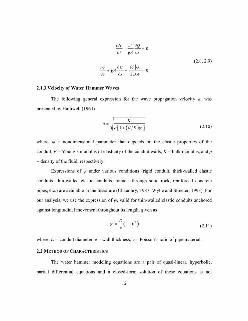
2.1.3 Velocity of Water Hammer Waves

The following general expression for the wave propagation velocity a, was

presented by Halliwell (1963)

a K

1 K E

(2.10)

where, ψ = nondimensional parameter that depends on the elastic properties of the

conduit, E = Young’s modulus of elasticity of the conduit walls, K = bulk modulus, and ρ

= density of the fluid, respectively.

Expressions of ψ under various conditions (rigid conduit, thick-walled elastic

conduits, thin-walled elastic conduits, tunnels through solid rock, reinforced concrete

pipes, etc.) are available in the literature (Chaudhry, 1987; Wylie and Streeter, 1993). For

our analysis, we use the expression of ψ, valid for thin-walled elastic conduits anchored

against longitudinal movement throughout its length, given as

D

e1

2 (2.11)

where, D = conduit diameter, e = wall thickness, ν = Poisson’s ratio of pipe material.

2.2 METHOD OF CHARACTERISTICS

The water hammer modeling equations are a pair of quasi-linear, hyperbolic,

partial differential equations and a closed-form solution of these equations is not

13

available. However, there are several methods to numerically integrate these equations,

such as, method of characteristics, explicit and implicit finite-difference methods, finite-

element methods, etc. Amongst these, the method of characteristics has been the most

popular due to its several advantages over other methods, particularly in water hammer

type problems. These advantages include an explicit form of solution such that different

elements can be solved independently and complex pipe networks can be handled with

ease, an established stability criterion, an easy to program and computationally efficient

procedure and most importantly, accurate solutions. The main disadvantage of this

method is the requirement to adhere to the time step-distance interval relationship.

The momentum and continuity equations, in terms of two dependent variables,

discharge and piezometric head, and two independent variables, distance along the pipe

and time, are transformed into four ordinary differential equations by the method of

characteristics. For further discussion let us rewrite the momentum and continuity

equations (Eqs. 2.8 and 2.9) as

L1Q

t gA

H

xfQ Q

2DA 0

L2 a

2 Q

x gA

H

t 0

(2.12, 2.13)

A linear combination of these equations using an unknown multiplier λ yields

L L1 L

2

Q

t a

2 Q

x

gA

H

x

1

H

t

fQ Q

2DA 0

(2.14)

Please note that, using any two real, distinct values of λ, Eq. (2.14) will again

yield two equations that are equivalent to Eqs. (2.12) and (2.13). Also, if H H (x, t )

and Q Q (x, t ) , then the total derivative can be written as

14

dH

dtH

tH

x

dx

dt

dQ

dtQ

tQ

x

dx

dt

(2.15, 2.16)

It can be seen by from Eqs. (2.14), (2.15) and (2.16), that if λ is defined as

1

dx

dt a

2

i.e., 1

a

(2.17)

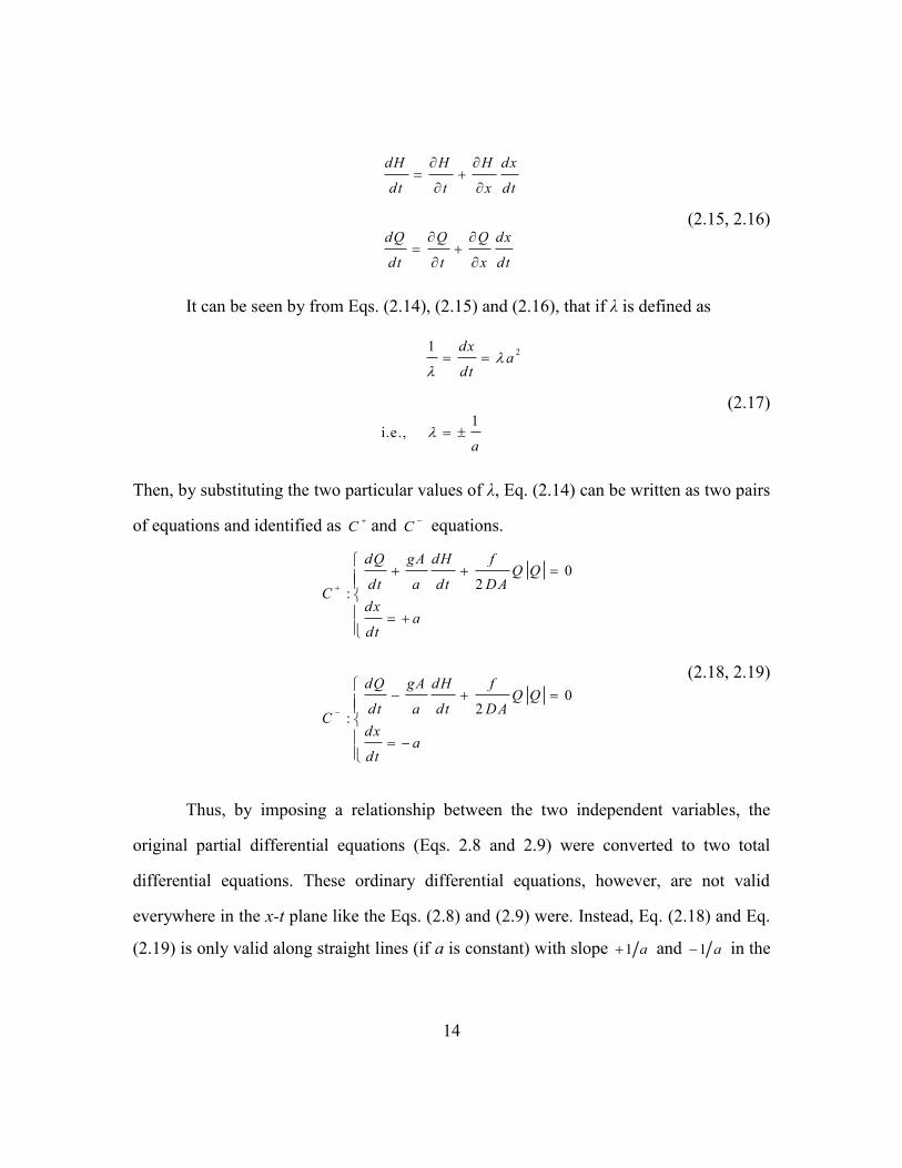
Then, by substituting the two particular values of λ, Eq. (2.14) can be written as two pairs

of equations and identified as C and C equations.

C

:

dQ

dtgA

a

dH

dt

f

2DAQ Q 0

dx

dt a

C

:

dQ

dtgA

a

dH

dt

f

2DAQ Q 0

dx

dt a

(2.18, 2.19)

Thus, by imposing a relationship between the two independent variables, the

original partial differential equations (Eqs. 2.8 and 2.9) were converted to two total

differential equations. These ordinary differential equations, however, are not valid

everywhere in the x-t plane like the Eqs. (2.8) and (2.9) were. Instead, Eq. (2.18) and Eq.

(2.19) is only valid along straight lines (if a is constant) with slope 1 a and 1 a in the

15

x-t plane, respectively. These lines are called characteristic lines and are shown in Fig.

2.1.

Figure 2.1: Characteristic grid in the x-t plane.

Physically, these lines represent the path travelled by a disturbance. For example,

a disturbance at point A (Fig. 2.2) at time t0 would travel to point P after time t .

Thus, we now have two ordinary differential equations and two unknowns, head

H and discharge Q. The unknowns can be calculated at all the points of intersection of the

characteristic lines, by integrating the differential equations in finite difference form and

solving them simultaneously.

t

x Δx = aΔt

Δt

C+ characteristic lines

C- characteristic lines

16

Figure 2.2: Characteristic lines in the x-t plane.

2.2.1 Finite Difference Equations

A pipeline is divided into an even number of reaches, n, each Δx in length as

shown in Fig. 2.1. A time-step is fixed at, Δt = a Δx. If the dependent variables, H and Q,

are known at A (Fig. 2.2) then Eq. (2.18), which is valid along the positively sloped

diagonal (C characteristic line) can be integrated along AP and expressed in terms of the

unknown H and Q at P. Similarly, with conditions known at B, Eq. (2.19) valid along the

C characteristic, can be integrated to yield a second equation in terms of the same

unknown H and Q at P.

dHH A

H P

a

gAdQ

QA

QP

f

2gDA2

Q QxA

xP

dx 0 (2.20)

The last term in this integration is unknown a priori, and can be written as a first-

order approximation as

Q QxA

xP

dx QAQA

(xP x

A)

(2.21)

or, as a second-order approximation as

Q QxA

xP

dx QPQA

(xP x

A)

(2.22)

t

x

A B

P

i –1 i i +1

t

t + Δt

17

The second-order approximation was used in this analysis, and after integrating as

explained, the two difference equations become

C

: HP H

A B (Q

P Q

A) RQ

PQA

(2.23)

C

: HP H

B B (Q

P Q

B) RQ

PQB (2.24)

where, B is the pipeline characteristic impedance:

B a

gA

(2.25)

and, R is the pipeline resistance coefficient:

R f x

2gDA2

(2.26)

The friction factor f is calculated by the Chen equation (Chen, 1979) at each time

step during calculations.

1

f 2 log

1

3.7065

e

D

5.0452

R elog

1

2.8257

e

D

1.1098

5.8506

R e0.8981

(2.27)

where, e = pipe roughness, D = pipe diameter and Re = local Reynolds number calculated

at every section at each time step.

The solution to a problem begins at steady-state conditions at time t = 0, so H and

Q at each section in the pipe is known. The solution proceeds by calculating H and Q at

any grid intersection point i at time t = Δt, from the known conditions at points i-1 and

i+1 from the preceding time step, t = 0 (as shown in Fig. 2.2). Thus, Eqs. (2.23) and

(2.24) may be written as,

C

: Hi

t t C

P B

PQt t

i (2.28)

18

C

: Hi

t t C

M B

MQi

t t

(2.29)

CP H

i 1

t BQ

t

i 1 (2.30)

BP B R Q

t

i 1 (2.31)

CM H

t

i 1 BQ

t

i 1 (2.32)

BM B R Q

t

i 1 (2.33)

where, subscript i refers to any grid intersection point, CP

, BP

, CM

and BM

are known

constants. Solving them simultaneously,

Hi

t tCPBM C

MBP

BP B

M

(2.34)

Qi

t tCP C

M

BP B

M (2.35)

However, at the end points of the grid, only one of the characteristics equations is

available, hence another relationship between H and Q must be provided to yield a

simultaneous equation. These relationships are called boundary conditions.

2.2.2 Nomenclature

So far, we had been dealing with single pipe systems. Before we go further, it is

necessary to explain the nomenclature scheme, used in this analysis, to reference

variables (shown in Fig. 2.3). To model a complete well, it is often necessary to describe

the well diagram as conduits or pipes with different properties (diameters, wall thickness,

etc.) connected in series. The first subscript refers to the conduit number (also referred to

19

as section number). Furthermore, each section or conduit is divided into a number of

reaches or subsections for the finite difference calculations. The second subscript refers

to the number of the subsection within a particular section. Finally, the superscript, if

included, refers to the time step of the calculation.

Figure 2.3: Nomenclature scheme for water hammer analysis.

2.3 BOUNDARY CONDITIONS

It can be seen from Fig. 2.1 that at the ends of a pipe, only one of the

characteristic equations is available. For the upstream end, the characteristic is

available, and for the downstream end, the characteristic is present. To calculate

pressure and discharge at the ends, another relationship is necessary that specifies

HP

, QP

or some relation between them (Fig. 2.2). Any text on water hammer discusses

various boundary conditions such as pumps, valves, orifice, etc., and their formulation.

For our analysis, we only deal with three boundary conditions that are a) flowrate as a

specified function of time at upstream end, b) series connection at the junction of pipes

with different properties (diameter, roughness, thickness, etc.) and, c) a porous

media/formation at the downstream end.

n+1 n n-1 n-2

Conduit i

Conduit i+1

1 2 3 4

Hi 1, 2

t

20

2.3.1 Flowrate as a Specified Function of Time at Upstream End

The change in flow at the upstream end due to the closing of a valve has been

expressed as a function of time. The opening or closing of a valve may be represented by

specifying τ versus t (as shown in Fig. 2.4) in a tabular form or as an analytical

expression, where τ is the fractional area of the valve open and t is time.

Figure 2.4: Valve opening and closing as a function of time.

The discharge, Q, through the valve is then expressed as,

Q1,1

t Q

0 (t ) (2.36)

where, Q0 is the steadystate flowrate. The other equation, valid at this point, is Eq. (2.28),

and together they may be solved to determine the unknown variables at every time step.

2.3.2 Series Connection

A series connection describes the junction of two conduits having different

diameters, wall thicknesses, materials and/or friction factors as shown in Fig. 2.4. If the

head losses at the junction are neglected, then it follows that

Hi , n 1

Hi 1, 1

(2.37)

τ

t

1

0 Fra

ctio

na

l A

rea o

f

Valv

e O

pen

, τ

Time, t

1

0

21

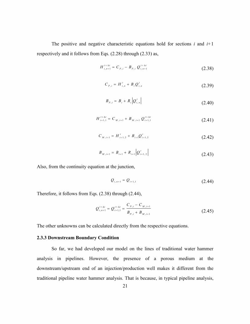
The positive and negative characteristic equations hold for sections i and i+1

respectively and it follows from Eqs. (2.28) through (2.33) as,

Hi , n 1

t t C

P , i B

P , iQi , n 1

t t (2.38)

CP , i

Hi , n

t B

iQi , n

t

(2.39)

BP , i

Bi R

iQi , n

t

(2.40)

Hi 1, 1

t t C

M , i 1 B

M , i 1Qi 1, 1

t t

(2.41)

CM , i 1

Hi 1, 2

t B

i 1Qi 1, 2

t

(2.42)

BM , i 1

Bi 1

Ri 1Qi 1, 2

t

(2.43)

Also, from the continuity equation at the junction,

Qi , n 1

Qi 1, 1

(2.44)

Therefore, it follows from Eqs. (2.38) through (2.44),

Qi , n 1

t t Q

i 1, 1

t tCP , i

CM , i 1

BP , i

BM , i 1

(2.45)

The other unknowns can be calculated directly from the respective equations.

2.3.3 Downstream Boundary Condition

So far, we had developed our model on the lines of traditional water hammer

analysis in pipelines. However, the presence of a porous medium at the

downstream/upstream end of an injection/production well makes it different from the

traditional pipeline water hammer analysis. That is because, in typical pipeline analysis,

22

the behavior of the boundary elements (such as pumps, surge tanks, orifices, valves etc.)

is well defined. On the other hand, the physical properties of the formation are not only

heterogeneous but also uncertain. The boundary condition must also describe the

transient response of the formation to a high-frequency pressure or rate wave at the sand

face. Thus, the conventional equations of pressure response used for pressure transient

analysis are unsuitable for this analysis, as they assume a step-change to constant rate or

pressure. Theoretically, the one-dimensional radial diffusivity equation, Eq. (2.46), can

be used but that would require us to assume radial flow (no fracture present), numerically

solve a second-order partial differential equation at every time step, estimate reservoir

properties and also make assumptions about the near well-bore pressure profile in the

reservoir.

2P

r2

1

r

P

rc

t

k

P

t (2.46)

where, is the formation porosity, is the fluid viscosity, ctis the total compressibility

of the system and k is the formation permeability.

In order to overcome these challenges, the formation was defined as an equivalent

electrical circuit with lumped resistive (R), capacitance (C) and inertance/inductance (I)

elements. A boundary condition can be defined in the form of Eq. (2.47) and the exact

formula of the function f depends on the combination (series, or parallel or a combination

of both) of R, C and I required to define the boundary.

H

Q f R ,C , I

(2.47)

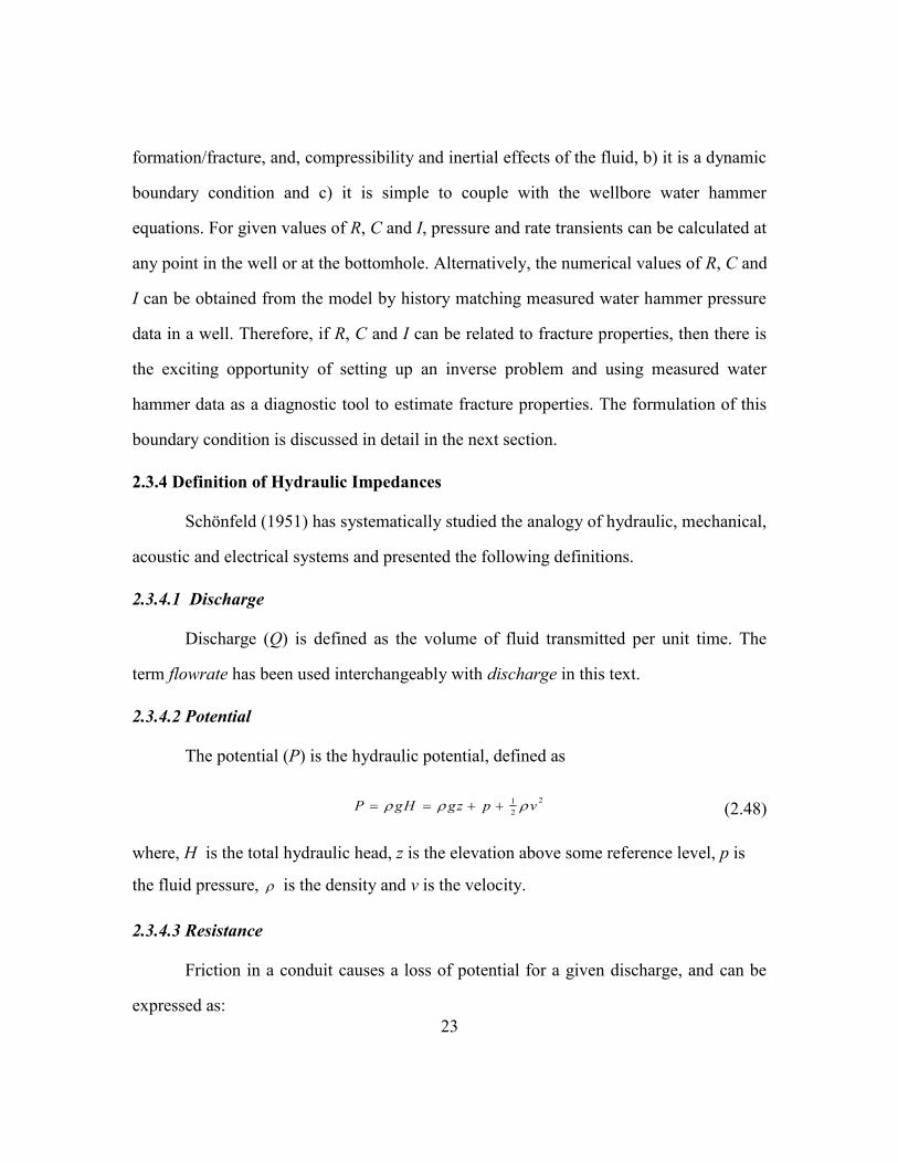
This definition has three distinct advantages: a) it accounts for the important

characteristics of the formation – resistance to flow, compliance of the

23

formation/fracture, and, compressibility and inertial effects of the fluid, b) it is a dynamic

boundary condition and c) it is simple to couple with the wellbore water hammer

equations. For given values of R, C and I, pressure and rate transients can be calculated at

any point in the well or at the bottomhole. Alternatively, the numerical values of R, C and

I can be obtained from the model by history matching measured water hammer pressure

data in a well. Therefore, if R, C and I can be related to fracture properties, then there is

the exciting opportunity of setting up an inverse problem and using measured water

hammer data as a diagnostic tool to estimate fracture properties. The formulation of this

boundary condition is discussed in detail in the next section.

2.3.4 Definition of Hydraulic Impedances

Schönfeld (1951) has systematically studied the analogy of hydraulic, mechanical,

acoustic and electrical systems and presented the following definitions.

2.3.4.1 Discharge

Discharge (Q) is defined as the volume of fluid transmitted per unit time. The

term flowrate has been used interchangeably with discharge in this text.

2.3.4.2 Potential

The potential (P) is the hydraulic potential, defined as

P gH gz p 1

2v

2 (2.48)

where, H is the total hydraulic head, z is the elevation above some reference level, p is

the fluid pressure, is the density and v is the velocity.

2.3.4.3 Resistance

Friction in a conduit causes a loss of potential for a given discharge, and can be

expressed as:

24

P RQ (2.49)

where, R 8 l r4 for laminar flow in a round tube of radius r. The factor R is called

the hydraulic resistance.

For linear flow through a porous medium,

P l

kA

Q RQ

(2.50)

Therefore, the flow Resistance (R) is the proportionality constant between the

discharge (Q) and the potential difference (P) that is required to maintain that discharge.

2.3.4.4 Capacitance

Consider a change in the volume of liquid stored in a system (V) for a change in

potential (P). Hence, V=CP or

Q CdP

dt (2.51)

where, the factor C is the Capacitance or the storage of the system.

2.3.4.5 Inertance

Consider a variable discharge through a tube. Ignoring friction for the moment, a

potential difference (P) will be required to accelerate or decelerate the flow. The

pressure drop required to accelerate the fluid is proportional to the inertance of the

system.

P IdQ

dt (2.52)

where, the factor I is the Inertance of the system.

25

2.3.4.6 Wellbore Impedance

The simplified equations of fluid transients in a pipeline were written as Eq. (2.8)

and Eq. (2.9). By comparing with the above-mentioned definitions, the resistance,

capacitance, and inertance for the wellbore may be written as follows. The impedances

are with respect to hydraulic head (H) and per unit length.

Rw

8w

rw

4 (2.53)

Cw gr

w

2

aw

2 (2.54)

Iw

1

grw

2

(2.55)

2.3.5 Analogous Electrical Circuit Representation

In order to draw the analogous electrical circuit representation of the

formation/fracture, it is essential to understand the pressure and flowrate behavior during

different operations and flow regimes. It is our primary interest to model water hammer

observed at the end of pumping in minifracs and after injector shut-ins.

Fig. 2.5 is the conceptual schematic of a wellbore connected to a fracture after a

minifrac job. The fracture is filled with the wellbore fluid without any proppant. There is

also filter cake deposition on the fracture walls to minimize leakoff and the flow regime

inside the fracture is linear. Also, injection at a steady bottomhole pressure implies a

growing fracture and in case the fracture stops growing, the bottomhole injection pressure

would increase sharply to maintain the injection rate. Therefore, it can be reasonably

assumed that during a minifrac, it is the fluid in the fracture and the volume of the

fracture that dominates the pressure-flowrate behavior. This can be represented by a

26

series combination of R, C and I as shown in Fig. 2.6. In this representation, current (~

flowrate) will stop in the circuit as soon as the capacitor (~ fracture compliance) is

charged. Current can keep flowing in the circuit, only if the potential difference (~ net

pressure) is increased, or, the impedance of the circuit is decreased. Therefore, an

increasing capacitance (~ growing fracture) will mean that current (~ frac fluid) can flow

in the circuit (~ fracture) at a constant potential difference (~ net pressure). This is

analogous to the pressure-flowrate behavior observed during minifracs. Eq. (2.56) is thus

the formulation of the bottomhole boundary condition (Eq. 2.47) for minifracs.

gH RQ 1

CQ dt I

dQ

dt

(2.56)

where, H is the potential difference, and Q is the flow rate.

Figure 2.5: Schematic of a minifrac connected to a wellbore.

27

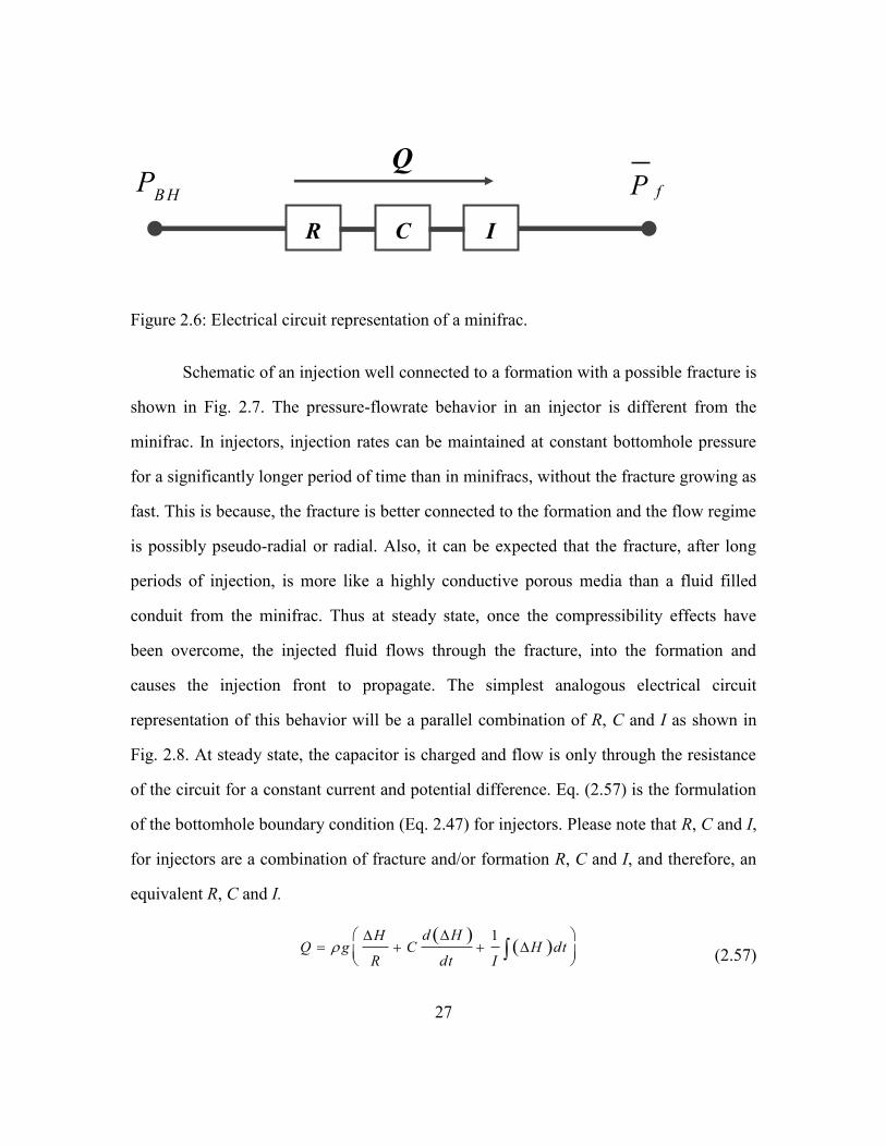
Figure 2.6: Electrical circuit representation of a minifrac.

Schematic of an injection well connected to a formation with a possible fracture is

shown in Fig. 2.7. The pressure-flowrate behavior in an injector is different from the

minifrac. In injectors, injection rates can be maintained at constant bottomhole pressure

for a significantly longer period of time than in minifracs, without the fracture growing as

fast. This is because, the fracture is better connected to the formation and the flow regime

is possibly pseudo-radial or radial. Also, it can be expected that the fracture, after long

periods of injection, is more like a highly conductive porous media than a fluid filled

conduit from the minifrac. Thus at steady state, once the compressibility effects have

been overcome, the injected fluid flows through the fracture, into the formation and

causes the injection front to propagate. The simplest analogous electrical circuit

representation of this behavior will be a parallel combination of R, C and I as shown in

Fig. 2.8. At steady state, the capacitor is charged and flow is only through the resistance

of the circuit for a constant current and potential difference. Eq. (2.57) is the formulation

of the bottomhole boundary condition (Eq. 2.47) for injectors. Please note that R, C and I,

for injectors are a combination of fracture and/or formation R, C and I, and therefore, an

equivalent R, C and I.

Q gH

R C

d H

dt

1

IH dt

(2.57)

R C I

P fPBH

Q

28

Figure 2.7: Schematic of an injection well.

Figure 2.8: Electrical circuit representation of an injector.

R C I

P f

PBH

Q

29

The potential difference, H , is defined in Eq. (2.47) as the difference between

the bottomhole pressure ( PBH

) and the average near wellbore pressure ( P f ) at any time.

Traditionally, the ISIP is considered to be the average near wellbore pressure because it is

assumed that the fluid comes to rest at shut-in and the near wellbore frictional pressure

drop, ( PBH - ISIP), becomes zero. But, the fluid in the wellbore does not come to rest

instantaneously (as proved by a water hammer). Hence, the traditional estimate of ISIP is

not completely devoid of the frictional pressure drop and thus not an accurate estimate of

the average near wellbore pressure. Therefore, average near wellbore pressure ( P f ) is

taken to be different from ISIP.

Water hammer is a fast transient as compared to the pressure transient response of

the reservoir. It is a reasonable assumption that the water hammer will not see the far-

field reservoir pressure. Hence, the potential difference has been defined with respect to

the average near wellbore pressure and not the average reservoir pressure. P f is

calculated by fitting an exponential decay curve to the decline part of the measured

surface pressure data, where k is the exponential decay constant and Pf 0

is the average

near wellbore pressure prior to shut-in.

gH P

BH P f

gHN ,n 1

t t P

f 0e kt

(2.58)

A conceptual schematic of this is shown in Fig. 2.9. The value of Pf 0

is always

between the instantaneous shut-in pressure (ISIP) and the end of water hammer pressure

( PEoWH

). If the pressure decline rate is low, then PEoWH

has been found to be a good

estimate of Pf 0

.

This completes the modeling of water hammer in the wellbore. In summary, the

inputs that must be provided are the injection fluid properties, the steady state injection

30

pressure and flowrate, the wellbore geometry specified as a series connection of different

pipes and the valve closing characteristics. The bottomhole boundary condition

parameters (R, C and I) can be either specified or obtained by history matching the

measured data (injection or minifrac water hammer). The model can then be used to

estimate bottomhole water hammer pressures.

Figure 2.9: Schematic of water hammer decline and near wellbore average pressure.

2.4 FRACTURE IMPEDANCE

2.4.1 Fracture Dimensions from Model Parameters

Once the values of the model parameters (R, C and I) have been estimated by

history matching the measured water hammer data, they can be used to calculate fracture

dimensions and net fracture overpressures by making the following assumptions:

ISIP

PEoWH

Pf 0e kt

Mea

sure

d S

urf

ace

Pre

ssu

re

Time

31

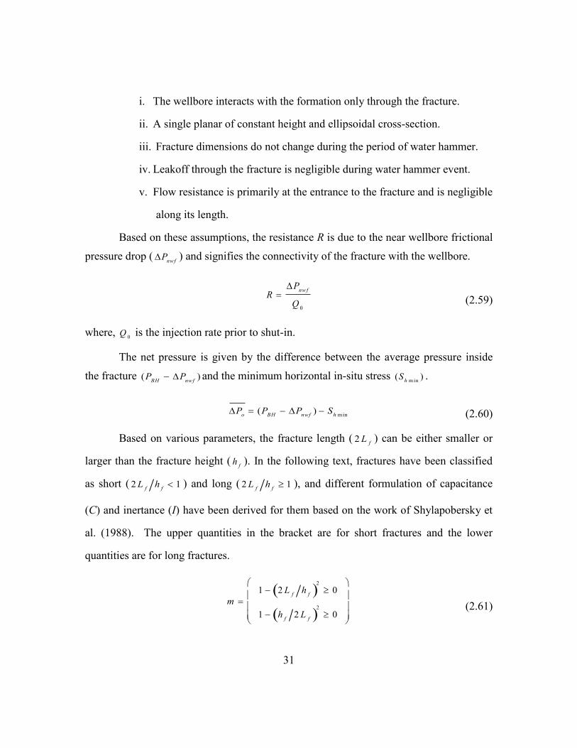
i. The wellbore interacts with the formation only through the fracture.

ii. A single planar of constant height and ellipsoidal cross-section.

iii. Fracture dimensions do not change during the period of water hammer.

iv. Leakoff through the fracture is negligible during water hammer event.

v. Flow resistance is primarily at the entrance to the fracture and is negligible

along its length.

Based on these assumptions, the resistance R is due to the near wellbore frictional

pressure drop ( Pnwf

) and signifies the connectivity of the fracture with the wellbore.

R P

nwf

Q0

(2.59)

where, Q0 is the injection rate prior to shut-in.

The net pressure is given by the difference between the average pressure inside

the fracture (PBH

Pnwf

) and the minimum horizontal in-situ stress (Sh m in

) .

Po (P

BH P

nwf) S

h min (2.60)

Based on various parameters, the fracture length ( 2 Lf) can be either smaller or

larger than the fracture height ( hf). In the following text, fractures have been classified

as short ( 2Lfhf 1 ) and long ( 2L

fhf 1 ), and different formulation of capacitance

(C) and inertance (I) have been derived for them based on the work of Shylapobersky et

al. (1988). The upper quantities in the bracket are for short fractures and the lower

quantities are for long fractures.

m

1 2 Lfhf

2

0

1 hf

2 Lf

2

0

(2.61)

32

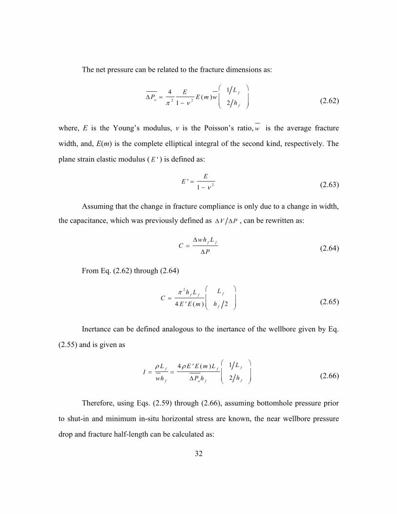
The net pressure can be related to the fracture dimensions as:

P

o

4

2

E

1 2E (m )w

1 Lf

2 hf

(2.62)

where, E is the Young’s modulus, ν is the Poisson’s ratio,w is the average fracture

width, and, E(m) is the complete elliptical integral of the second kind, respectively. The

plane strain elastic modulus ( E ' ) is defined as:

E ' E

1 2

(2.63)

Assuming that the change in fracture compliance is only due to a change in width,

the capacitance, which was previously defined as V P , can be rewritten as:

C wh

fLf

P (2.64)

From Eq. (2.62) through (2.64)

C

2hfLf

4 E 'E (m )

Lf

hf

2

(2.65)

Inertance can be defined analogous to the inertance of the wellbore given by Eq.

(2.55) and is given as

I

Lf

whf

4 E 'E (m )L

f

Pohf

1 Lf

2 hf

(2.66)

Therefore, using Eqs. (2.59) through (2.66), assuming bottomhole pressure prior

to shut-in and minimum in-situ horizontal stress are known, the near wellbore pressure

drop and fracture half-length can be calculated as:

33

Pnwf

RQ0

(2.67)

Lf

CI Po

(2.68)

Since, E(m) and w are functions of fracture height, hfand w are calculated

iteratively by such that Eqs. (2.69) and (2.70) are satisfied.

2 2

2

4 ' ( )2 1

8 ' ( )2 1

f f

f

f

f f

f

E E m Cif L h

L

hE E m C

if L hL

(2.69)

hfL

f

wI (2.70)

2.4.2 Estimate of Model Parameters

An initial estimate of R, C and I can be made from estimates/assumptions of

fracture height and near wellbore frictional pressure drop. The fracture height may be

assumed to be the height of the perforated interval. The near wellbore frictional pressure

drop, Pnwf

, may be calculated as:

Pnw f

PBH

t 0 P

f 0 (2.71)

R can be estimated according to Eq. (2.60). To calculate C and I, estimates of

w and Lf must first be obtained.

Shylapobersky et al. (1988) formulated an expression for average width by taking

into consideration the width due to both viscous dissipation (wf) and rock toughness

34

(wc) effects. In order to distinguish it from the average width definition used previously

(w ), this definition of average width will be referred to as w ' and is given by:

w ' wc

2 w

c

4 w

f

4 (2.72)

where,

wc

2

2

4E 'E (m )

LfGs(m )

hf

2Gl(m )

(2.73)

wf

4

34Q

0Lf

8E 'E (m )

Lfhf

1 2

(2.74)

The geometrical function for short fracture and long fracture is given by:

Gs(m )

Gl(m )

1.0 2 Lfhf

2

K (m ) E (m ) 2mE (m )

0.5 hf

2 Lf

2

K (m ) E (m ) 2mE (m )

(2.75)

where, K(m) and E(m) are the complete elliptical integral of the first and second kind,

respectively (Appendix).

The apparent fracture toughness (Γ) is given for short and long fractures as:

s

l

2 Po

2

Lf

E '

2P

o 2

hfGl(m )

32E 'E (m )

(2.76)

The fracture length is calculated iteratively by equating the two average widths

given by Eq. (3.62) and (3.72) respectively. The average fracture width can then be

35

calculated either definition. Initial estimates of R, C and I can be obtained to run the

water hammer model. These estimates can be improved by iteratively matching the

measured water hammer data.

36

Chapter 3: Results and Discussion

3.1 HYDRAULIC IMPEDANCE TESTING

To validate our modeling approach, this model was used to simulate a hydraulic

impedance test. Instead of a shut-in at the surface (a step change in flowrate), a short

duration pressure pulse was generated by momentarily changing the flowrate at the

surface. Figs. 3.1 and 3.2 show the results for an open fracture (low resistance, high

capacitance) and a closed fracture (high resistance, low capacitance) respectively. The

results show that for an open fracture the pressure wave is reflected with an opposite

polarity while for a closed fracture the reflected wave has the same polarity as that of the

incident wave. This is a well-known observation (Holzhausen et al., 1985; Patzek and De,

2000) and forms the basis of using pressure pulse testing to determine fracture closure

pressures. In this case, it confirms that our modeling approach (which is traditional fluid

transient analysis by solving conservation of mass and momentum equations but with an

impedance boundary condition) can adequately capture the wellbore-fracture dynamics.

37

Figure 3.1: Simulated HIT for well with open fracture.

Figure 3.2: Simulated HIT for well with closed fracture.

38

3.2 HISTORY MATCHING SURFACE WATER HAMMER IN INJECTORS

The model was used to simulate several injector water hammer incidents from

different fields. In this text we will discuss five injector water hammer cases that were

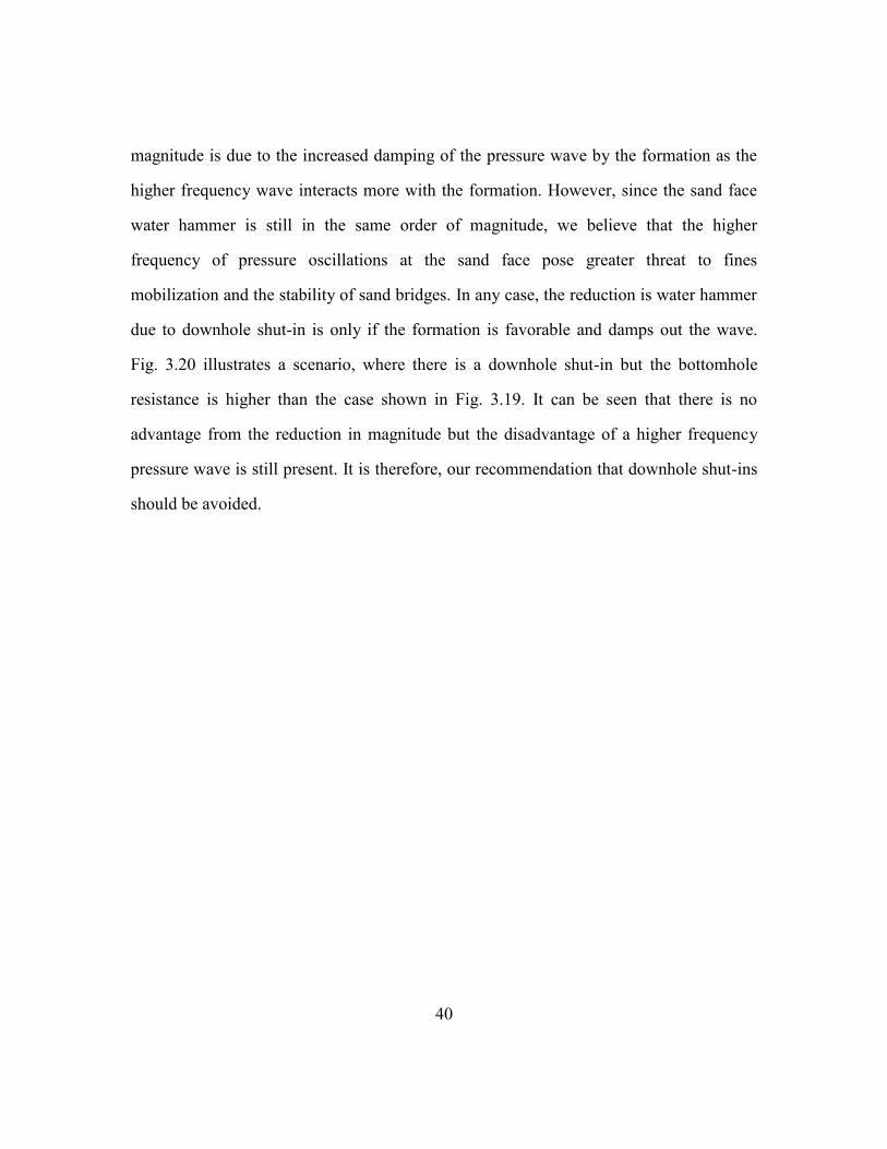
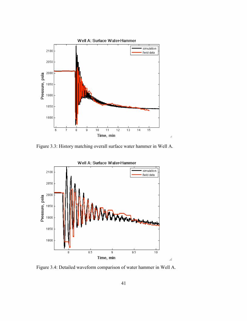
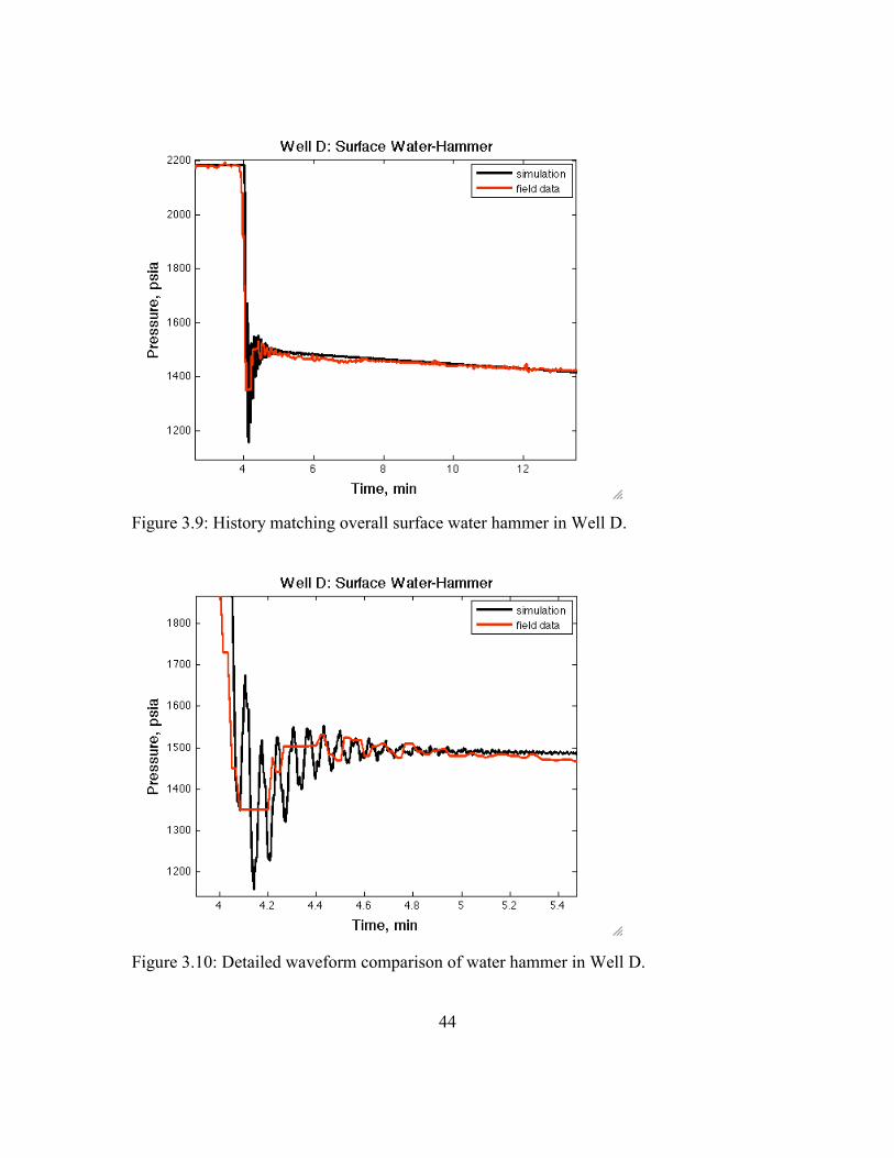
presented by McCarty and Norman (2006). Figs. 3.3 through 3.12 show two plots for

each well A through E, respectively. The first figure for each case shows the overall

match (amplitude, decay and duration) of the water hammer incident, while the second

offers a closer look at the water hammer data and highlights the detailed waveform

comparison.

It can be seen that the model shows a good agreement with the measured data for

a wide variety of water hammer situations. Wells A, B, and E, in particular, show

remarkable agreement between the model and the data. Though the model predicts the

overall trend for wells C and D, a closer look at the data reveals that some waveforms are

truncated and some apparent wave cycles have been missed in the measurements. This

can be attributed to the sensitivity and sampling time of the pressure gauge used to collect

the data. As illustrated by Wang et al. (2008) (Fig. 3.13), under-sampling can distort the

data and give the impression of longer wave periods or lower frequency of oscillations

than might be the actual case. Also, under-sampling can miss some of the pressure peaks

showing lower amplitudes. We see evidence of both from the comparison of the modeled

water hammer to the measured data. Therefore, it is recommended to use faster gauges to

capture the full details of a water hammer. Ideally, a pressure gauge that can at least

sample at twice the frequency of the water hammer wave should be used.

3.3 SIMULATED BOTTOMHOLE WATER HAMMER IN INJECTORS

Figs. 3.14 through 3.18, show the simulated bottomhole water hammer for these

cases. It can be observed that in all these cases, the bottomhole water hammer magnitudes

are lower than the surface values. The sand face water hammer is in tens of psi whereas

39

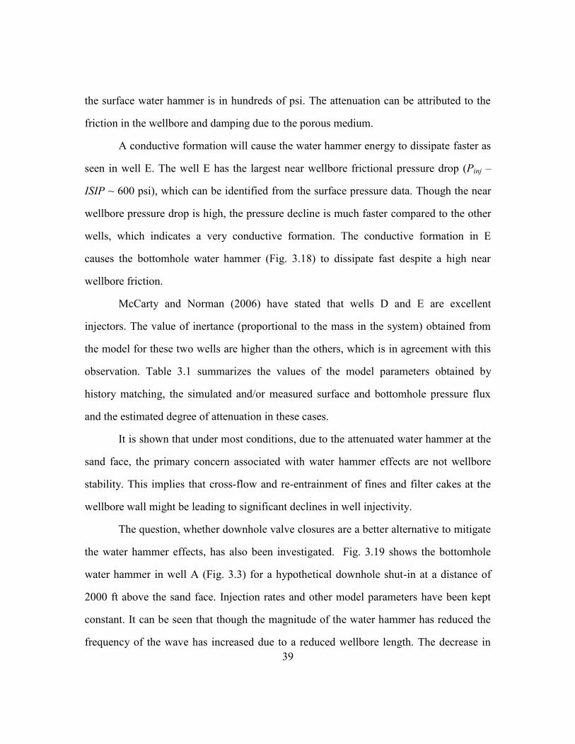
the surface water hammer is in hundreds of psi. The attenuation can be attributed to the

friction in the wellbore and damping due to the porous medium.

A conductive formation will cause the water hammer energy to dissipate faster as

seen in well E. The well E has the largest near wellbore frictional pressure drop (Pinj –

ISIP ~ 600 psi), which can be identified from the surface pressure data. Though the near

wellbore pressure drop is high, the pressure decline is much faster compared to the other

wells, which indicates a very conductive formation. The conductive formation in E

causes the bottomhole water hammer (Fig. 3.18) to dissipate fast despite a high near

wellbore friction.

McCarty and Norman (2006) have stated that wells D and E are excellent

injectors. The value of inertance (proportional to the mass in the system) obtained from

the model for these two wells are higher than the others, which is in agreement with this

observation. Table 3.1 summarizes the values of the model parameters obtained by

history matching, the simulated and/or measured surface and bottomhole pressure flux

and the estimated degree of attenuation in these cases.

It is shown that under most conditions, due to the attenuated water hammer at the

sand face, the primary concern associated with water hammer effects are not wellbore

stability. This implies that cross-flow and re-entrainment of fines and filter cakes at the

wellbore wall might be leading to significant declines in well injectivity.

The question, whether downhole valve closures are a better alternative to mitigate

the water hammer effects, has also been investigated. Fig. 3.19 shows the bottomhole

water hammer in well A (Fig. 3.3) for a hypothetical downhole shut-in at a distance of

2000 ft above the sand face. Injection rates and other model parameters have been kept

constant. It can be seen that though the magnitude of the water hammer has reduced the

frequency of the wave has increased due to a reduced wellbore length. The decrease in

40

magnitude is due to the increased damping of the pressure wave by the formation as the

higher frequency wave interacts more with the formation. However, since the sand face

water hammer is still in the same order of magnitude, we believe that the higher

frequency of pressure oscillations at the sand face pose greater threat to fines

mobilization and the stability of sand bridges. In any case, the reduction is water hammer

due to downhole shut-in is only if the formation is favorable and damps out the wave.

Fig. 3.20 illustrates a scenario, where there is a downhole shut-in but the bottomhole

resistance is higher than the case shown in Fig. 3.19. It can be seen that there is no

advantage from the reduction in magnitude but the disadvantage of a higher frequency

pressure wave is still present. It is therefore, our recommendation that downhole shut-ins

should be avoided.

41

Figure 3.3: History matching overall surface water hammer in Well A.

Figure 3.4: Detailed waveform comparison of water hammer in Well A.

42

Figure 3.5: History matching overall surface water hammer in Well B.

Figure 3.6: Detailed waveform comparison of water hammer in Well B.

43

Figure 3.7: History matching overall surface water hammer in Well C.

Figure 3.8: Detailed waveform comparison of water hammer in Well C.

44

Figure 3.9: History matching overall surface water hammer in Well D.

Figure 3.10: Detailed waveform comparison of water hammer in Well D.

45

Figure 3.11: History matching overall surface water hammer in Well E.

Figure 3.12: Detailed waveform comparison of water hammer in Well E.

46

Figure 3.13: Misrepresentation of water hammer data due to the effect of under-sampling

(after Wang et al., 2008).

Figure 3.14: Simulated bottomhole water hammer for well A

47

Figure 3.15: Simulated bottomhole water hammer for well B.

Figure 3.16: Simulated bottomhole water hammer for well C.

48

Figure 3.17: Simulated bottomhole water hammer for well D.

Figure 3.18: Simulated bottomhole water hammer for well E.

49

Wells Resistance

(bpd/psi)

Capacitance

(bbl/psi)

Inertance

(psi/bbl/d2)

ΔPSurface (psi)

(Simulation/Measured)

ΔPBH (psi)

(Simulation)

Attenuation

PBH

Psurface

A 89.87 2.44×10-3

3.09×10-7

350/265 50 0.14

B 333.9 6.72×10-3

2.45×10-8

850/660 60 0.07

C 74.75 3.29×10-3

3.09×10-7

470/350 60 0.13

D 59.38 1.09×10-3

1.23×10-6

300/180 60 0.20

E 94.11 2.74×10-3

9.77×10-7

500/500 70 0.14

Table 3.1: Summary of model parameters, total surface and bottomhole pressure fluxes and attenuation.

Wells Resistance

(bpd/psi)

Capacitance

(bbl/psi)

Inertance

(psi/bbl/d2)

Height

(ft)

Half Length

(ft)

Width

(in)

ΔPnwf

(psi)

A 89.87 2.44×10-3

3.09×10-7

4.3 403.3 0.05 94.5

B 333.9 6.72×10-3

2.45×10-8

10.2 198.2 0.12 52.4

C 74.75 3.29×10-3

3.09×10-7

4.7 468.9 0.05 93.6

D 59.38 1.09×10-3

1.23×10-6

3.5 283.5 0.01 387.3

E 94.11 2.74×10-3

9.77×10-7

4.1 507.8 0.02 318.8

Table 3.2: Summary of model parameters, equivalent fracture dimensions and near wellbore frictional pressure drop.

50

Figure 3.19: Simulated bottomhole water hammer for a downhole shut-in in well A.

Figure 3.20: Simulated bottomhole water hammer for a downhole shut-in in well A with

different formation properties.

51

3.4 FRACTURE DIAGNOSTICS IN INJECTORS

McCarty and Norman (2006) maintain that the injection pressure gradients in

these wells are below the adjusted fracture gradients after taking into consideration the

increased pore pressure due to several years of injection. In that case, the model cannot

calculate fracture dimensions, as injection pressures lower than the fracture pressures

violate the model formulation. However, to demonstrate the capabilities of the model,

equivalent fracture dimensions have been calculated by assuming that there exists a 500

psi net-pressure in all the wells, which is not necessarily true. The equivalent fracture

dimensions and near wellbore frictional pressure drop calculated from the model

parameters have been presented in Table 3.2. It can be seen that the near wellbore

frictional pressure drops (representative of the connectivity of the wellbore to the

formation) are in good agreement with the observed data. Please also note that these are

equivalent fracture dimension as per the assumptions of the model. These injectors are in

high permeability formations (~ 1000 to 2000 md) and therefore the resistance,

capacitance and inertance are also influenced by the formation as explained in the model

formulation.

A portable and easy-to-use tool was also created by implementing this model in

Excel VBA. The tool can be used to analyze the effects of different valve closure times,

injection rate, well geometry and valve positions, as wells as estimate equivalent fracture

dimensions from water hammer data for injectors or minifrac jobs.

3.5 FRACTURE DIAGNOSTICS FROM MINIFRAC DATA

Several minifrac jobs were also analyzed with this tool. The conditions in a

minifrac job (a single unpropped fracture and more accurate estimate of minimum

horizontal in-situ stress) are closer to the assumptions of the fracture model and make it a

better candidate for testing this model. Fig. 3.21 and 3.22 show the comparison of the

52

modeled and the measured tubing head pressure (THP) data and bottomhole pressure

(BHP) data for a minifrac job in an offshore well. The bottomhole pressure data (Fig.

3.22) shown in this case is at the sand face. It can be seen that the model accurately

predicts the sand face water hammer magnitude, frequency and waveform. The

discrepancy in the decline rate and the few extra cycles in the modeled results are due to

the viscoelastic frac fluid being modeled as a Newtonian fluid. The attenuation of the

water hammer to tens of psi at the sand face from approximately 1000 psi at the surface

should also be noted. This is a confirmation of our simulated attenuation in the injector

water hammer cases discussed previously.

The fracture dimensions calculated from the model have been compared to the

ones obtained from a commercial simulated in Table 3.3. It can be said that the fracture

dimensions are reasonable and comparable.

Table 3.3: Comparison of fracture dimensions obtained from model with dimensions

from fracture simulator for a minifrac job.

Fracture Dimensions Calculated from Model Calculated from E-Stimplan

Height (ft) 81.7 75

Half Length (ft) 69.3 35

Width (in) 0.13 0.22

53

Figure 3.21: Comparison of modeled and measured surface water hammer pressure for a

minifrac job.

Figure3.22: Comparison of modeled and measured bottomhole water hammer data for a

minifrac job.

54

Chapter 4: Conclusion

A pressure transient is generated when a sudden change in injection rate occurs

due to a valve closure or injector shutdown. This pressure transient, referred to as a water

hammer, travels down the wellbore, is reflected back and induces a series of pressure

pulses on the sand face. The resulting pressure surges can often lead to reduced

injectivity, cross flow between zones, sand face failure and sand production. This study

presents a semi-analytical model to simulate the magnitude, frequency and duration of

water hammer in wellbores, which can be used to understand its impact on wellbore

stability in poorly consolidated sands. A RCI model has been suggested that can describe

the interface, between the wellbore and the formation.

Pressure transients measured in five wells in an offshore field are history

matched with the model to obtain typical model parameters. It is shown that the model

accurately predicts the effect of injector rate, rate of shutdowns and other well

parameters. The implications for completion design and sand control in injectors are

discussed.

It is shown that the amplitude of the pressure waves may be up to an order of

magnitude smaller at the sand face when compared with surface measurements. This

suggests that sand failure may not be as big a concern as originally thought. However,

some concerns still remain.

The primary concerns in injectors may be a combination of the following factors.

The sand that is already in a failed state due to high rate injection may be liquefied and

sucked in to the wellbore due to pressure waves. A transient rate hammer accompanying

the pressure hammer may cause fines migration and mobilization, and failure of sand

bridges. Cross-flow induced by shut-in between unevenly charged layers can also cause

55

fines to enter the wellbore. If enough time is not allowed for fines and sand to settle prior

to reinjection, plugging of gravel packs and screen can lead to reduced injectivity.

Downhole valve closures should be avoided as they create a pressure wave of comparable

magnitude but much higher frequency than surface shut-ins, which can potentially cause

more damage.

Finally, a model has been proposed to estimate fracture dimensions from water

hammer data. The model has been used to obtain equivalent fracture dimensions from

injector and minifrac water hammer events. The model shows reasonable agreement with

fracture dimensions obtained from commercial simulators.

56

Appendix

The complete elliptical integral of the first kind K is defined as:

K m d

1 m2

sin2

0

2

dt

1 t2 1 m

2t

2 0

1

Numerically K can be approximated as

K 1 x c0 c

1x c

2x

2 d0 d

1x d

2x

2 log 1 x

where, c0 = 1.3862944, c1 = 0.1119723, c2 = 0.0725296, d0 = 0.5, d1 = 0.1213478, d2 =

0.0288729.

The complete elliptical integral of the second kind E is defined as:

E m 1 m

2sin

2 d

0

2

1 m

2t

2

1 t2 0

1

dt

Numerically E can be approximated as

E 1 x 1 a1x a

2x

2 b1x b

2x

2 log 1 x

where, a1 = 0.4630151, a2 = 0.2452727, b1 = 0.1077812, b2 = 0.0412496.

57

References

Afshar, M.H., Rohani, M. 2008. Water Hammer Simulation by Implicit Method of

Characteristics. International Journal of Pressure Vessels and Piping 85: 851-

859.

Allievi, L. 1902. General theory of the variable motion of water in pressure conduits.

Annali della Societa` degli Ingegneri ed Architetti Italiani 17(5): 285-325 (in

Italian). (French translation by Allievi, in evue de Me canique, Paris, 1904)

(Discussed by Bergant et al., 2006).

Allievi, L. 1913. Teoria del colpo d’ariete (Theory of water-hammer.). Atti del Collegio

degli Ingegneri ed Architetti Italiani, Milan, (in Italian) (Discussed by Bergant et

al., 2006).

Ashour, A.I.S. 1994. A Study of Fracture Impedance Method. Ph.D Dissertation. The

University of Texas at Austin, Austin.

Barr, D.I.H. 1980. The Transition from Laminar to Turbulent Flow. In: Proc. Instn. Civ.

Engrs., Part 2 69: 555-562.

Bergant, A., Simpson, A. ., Vı´tkovsky´, J. 2001. Developments in Unsteady Pipe Flow

Friction Modeling. Journal of Hydraulic Research 39(3): 249-257.

Bergant. A., Simpson, A.R., Tijsseling, A.S. 2006. Water Hammer with Column

Separation: A Historical Review. Journal of Fluids and Structures 22: 135-171.

Bergeron, . 1935. Etude des variations de re gime dans les conduites d’eau-Solution

graphique ge ne rale (Study on the Steady-State Variations in Water-Filled

Conduits-General Graphical Solution) (in French).

’Hy iq 1(1): 12-25. (Discussed in Saikia and Sarma, 2006).

Bergeron, . 1936. Estude des coups de beler dans les conduits, nouvel exose’ de la

methodegraphique. La Technique Moderne 28: 33. (Discussed in Saikia and

Sarma, 2006).

Brunone, B., Golia, U.M., Greco, M. 1991. Modeling of fast transients by numerical

methods. In: Proceedings of the International Meeting on Hydraulic Transients

with Column Separation. 9th Round Table, IAHR, Valencia, Spain. pp. 215-222.

Chaudhry, H.M., Hussaini, M.Y. 1985. Second-order Accurate Explicit Finite-Difference

Schemes for Water Hammer Analysis. Journal of Fluids Engineering 107: 523-

529.

Chaudhry, H.M. 1987. Applied Hydraulic Transients. 2nd

ed. Van Nostrand Reinhold

Company, New York.

Chen, N.H. 1979. An Explicit Equation for Friction Factor in Pipe. Ind. Eng. Chem.

Fund. 18: 296.

58

Ghidaoui, M.S., Mansour, G.S., Zhao, M. 2002. Applicability of Quasi Steady and

Axisymmetric Turbulence Models in Water Hammer. Journal of Hydraulic

Engineering 128(10): 917-924.

Greyvenstein, G.P. 2006. An Implicit Method for Analysis of Transient Flows in Piping

Networks. International Journal for Numerical Methods in Engineering 53: 1127-

1148.

Halliwell, A.R. 1963. Velocity of a Water Hammer Wave in an Elastic Pipe. ASCE

Journal of Hydraulic Division 89(4): 1-21.

Hayatdavoudi, A. 2006. Well Sanding and Lost Production Due to Cyclic Water

Hammer. Paper SPE 100928 presented at SPE Annual Technical Conference and

Exhibition, San Antonio, 24-27 September.

Holzhausen, C.R., Gooch, R.P. 1985. Impedance of Hydraulic Fracture: Its Measurement

and Use for Estimating Fracture Closure and Dimensions. Paper SPE 13892

presented at SPE/DOE Low Permeability Gas Reservoirs Symposium, Denver,

19-22 May.

Holzhausen, C.R., Egan, H.N. 1986. Fracture Diagnostics in East Texas and Western

Colorado using Hydraulic-Impedance Method. Paper SPE 15215 presented at the

SPE Unconventional Gas technology Symposium, Louisville, 18-21 May.

Hornaby, B.E., Johnson, D.L., Winker, K.W., Plumb, R.A. 1989. Fracture Evaluation

using Reflected Stoneley Wave Arrivals. Geophysics 54(10): 1274-1288.

Joukowsky, . 1900. n the Hydraulic Hammer in Water Supply Pipes. Me moires de

l’Acade mie Impe riale des Sciences de St.-Petersbourg 8(9): 5 (in German).

English translation by, Simin, 1904.

KSB Know-how, Volume 1: Water Hammer. 2006. KSB,

www.ksbpak.com/pdfs/waterhammer.pdf/ . Downloaded 10 November 2010.

Khalevin, N.I. 1960. Measurement of rock porosity by sonic well logging.

Razvedochnaya i Promyslovaya Geofizika 30: 3-9.

Mathieu, F., Toksoz, M.N. 1984. Application of Full Waveform Acoustic Logging Data

to the Estimation of Reservoir Permeability. Proceedings, Soc. of Exploration

Geophysicists 54th International Meeting, Atlanta. pp. 9-12.

McCarty, R.A., Norman, W.D. 2006. The Resiliency of Frac-Packed Subsea Injection

Wells. Paper SPE 102990 presented at SPE Annual Technical Conference and

Exhibition, San Antonio, 24-26 September.

Medlin, W.L. 1991. Fracture Diagnostics with Tube Wave Logs. Paper SPE 22872

presented at the 66th Annual Technical Conference and Exhibition, Dallas, 6-9

October.

59

Morris, R.L., Grine, D.R., Arkfeld, T.E. 1964. Using Compressing and Sheer Acoustic

Amplitudes foe Location of Fracture. Journal of Petroleum Technology 16: 623-

632.

Moos, D., Quan, Y. 2006. Methods and Devices for Analyzing and Controlling the

Propagation of Waves in a Borehole Generated by Water Hammer. US Patent No.

US2006/0293857A1.

Paige, R.W., Murray, I.R., Roberts, J.D.M., Mellor, D.W. 1992. Fracture Measurement

using Hydraulic Impedance Testing. Paper SPE 24824 presented at the 68th

Annual Technical Conference and Exhibition, Washington, DC, 4-7 October.

Paige, R.W., Murray, L.R., Roberts, J.D.M. 1993. Field Application of Hydraulic

Impedance Testing for Fracture Measurement. Paper SPE 26525 presented at the

SPE Annual Technical Conference and Exhibition, Houston, 3-6 October.

Parmakian, J. 1963. Water Hammer Analysis. Dover Publications, New York.

Patzek, T.W., De, A. 2000. Lossy Transmission Line Model of Hydrofractured Well

Dynamics. Journal of Petroleum Science and Engineering 25(1-2): 59-77.

Saikia, M.D., Sarma, A.K. 2006. Simulation of Water Hammer Flows with Unsteady

Friction Factor. ARPN Journal of Engineering and Applied Sciences 1(4): 35-40.

Santarelli, F.J., Skomedal, E., Markestad, P., Berge, H.I., Nasvig, H. 2000. Sand

Production on Water Injectors: Just How Bad Can It Get? SPE Drill. & Compl

15(2): 132.

Schönfeld, J.C. 1951. Analogy of Hydraulic, Mechanical, Acoustic and Electrical

Systems. Appl. Sci. Res. 3(B): 417-450.

Shimada, M., Okushima, S. 1984. New Numerical Model and Technique for Water

Hammer. Journal of Hydraulic Engineering 110(6): 736-748.

Shylapobersky, J., Wong, G.K., Walhaug, W.W. 1988. Overpressure Calibrated Design

of Hydraulic Fracture Stimulations. Paper SPE 18194 presented at the 63rd

SPE

Annual Technical Conference and Exhibition, Houston, 2-5 October.

Silva-Araya, W. 1993. Energy Dissipation in Transient Flow. Ph.D Dissertation.

Washington State University, Washington.

Silva-Araya, W., Chaudhry, M.F. 1997. Computation of Energy Dissipation in Transient

Flow. Journal of Hydraulic Engineering 123(2): 108-115.

Streeter, V.L., Wylie, E.B. 1967. Hydraulic Transients. McGraw Hill, New York.

Tang, X.M., Cheng, C.H. 1989. A Dynamical Model for Fluid Flow in Open Borehole

Fractures. Journal of Geophysical Research 94(B6): 7567-7576.

Trikha, A.K. 1975. An Efficient Method for Simulating Frequency-dependent Friction in

Transient Liquid Flow. Journal of Fluids Engineering 97: 97-105.

60

Vardy, A.E., Brown, J.M.B. 2004. Transient Turbulent Friction in Fully Rough Pipe

Flows. Journal of Sound and Vibration 270(1-2): 233-257.

Vardy, A.E., Hwang, K. 1991. A Characteristic Model of Transient Friction. Journal of

Hydraulics Research 29(5): 669-684.

Vaziri, H., Nouri, A., Hovem, K., Wang, X. 2007. Computation of Sand Production in

Water Injectors. Paper SPE 107695 presented at the European Formation Damage

Conference, Scheveningen, 30 May-1 June.

Walker, T. 1962. Fracture zones vary acoustic signal amplitudes. W. O. 154(6).

Wang, X., Hovem, K. 2008. Water Hammer Effects on Water Injection Well

Performance and Longevity. Paper SPE 112282 presented at the SPE

International Symposium and Exhibition on Formation Damage Control,

Lafayette, 13-15 February.

Wood, D.J. 2005a. Water Hammer Analysis – Essential and Easy (and Efficient). Journal

of Environmental Engineering 131(8): 341-348.

Wood, D.J., Lindireddy, S., Boulos, P.F., Karney, B., McPherson, D.L. 2005b. Numerical

Methods for Modeling Transient Flow. Journal of the American Water Works

Association 97(7): 104-115.

Wylie, E.B., Streeter, V.L. 1993. Fluid Transients in Systems. Prentice-Hall, New Jersey.

Zhao, M., Ghidaoui, M.S. 2003. Efficient Quasi Two Dimensional Model for Water

Hammer Problems. Journal of Hydraulic Engineering 1129(12): 1007-1013.

Zhao, M., Ghidaoui, M.S. 2004. Godunov-type Solutions for Water Hammer Flows.

Journal of Hydraulic Engineering 130(4):341-348.

Zielke, W. 1968. Frequency-dependent Friction in Transient Pipe Flow. Journal of Basic

Eng, ASME. 90(9): 109-115.