Copyright by Nevzat Onur Domani˘c 2017plaxton/pubs/dissertations/domanic.pdf · Nevzat Onur...

Copyright

by

Nevzat Onur Domanic

2017

The Dissertation Committee for Nevzat Onur Domaniccertifies that this is the approved version of the following dissertation:

Unit-Demand Auctions:

Fast Algorithms for Special Cases and a

Connection to Stable Marriage with Indifferences

Committee:

C. Gregory Plaxton, Supervisor

Vijaya Ramachandran

Eric Price

Evdokia Nikolova




by

Nevzat Onur Domanic

Dissertation

Presented to the Faculty of the Graduate School of

The University of Texas at Austin

in Partial Fulfillment

of the Requirements

for the Degree of

Doctor of Philosophy


August 2017

To my parents and my brother, who have been there from day one on this

journey; and to my nephew, who joined halfway through and caught up.

Acknowledgments

This dissertation would not have been possible without the guidance, insight,

and support of my adviser C. Gregory Plaxton. I would like to express my

deepest gratitude for the patient guidance and mentorship he provided during

this exciting endeavor. He is not only a source of constant encouragement and

inspiration, but also the perfect exemplar of unbounded kindness and positive

attitude. I cannot express how grateful and fortunate I am to have had him

as my adviser.

I would also like to thank the rest of my dissertation committee, Vijaya

Ramachandran, Eric Price, and Evdokia Nikolova, for their valuable comments

and feedback.

I am very grateful and lucky to have collaborated with Chi-Kit Lam, I

have learned a lot from our discussions and work together.

I would like to thank my fellow graduate students and the CS depart-

ment staff for their support and friendship. It has been a pleasure to be a

member of the graduate student community at UT.

I would like to thank my friends in Austin who made my stay here so

much more enjoyable. Special thanks to a few who made Austin a place to

call home, they know who they are!

v

Finally, and most importantly, I would like to thank my mother, Serpil,

my father, Yuksel, and my brother, Arman, for their continuous love and

support.

Nevzat Onur Domanic


August 2017

vi




by

Nevzat Onur Domanic, Ph.D.

The University of Texas at Austin, 2017

SUPERVISOR: C. Gregory Plaxton

Unit-demand auctions have been heavily studied, in part because this

model allows for a mechanism enjoying a remarkably strong combination of

game-theoretic properties: efficiency, stability (or envy-freeness), and strate-

gyproofness. One way to derive this mechanism is to specialize the Vickrey-

Clarke-Groves (VCG) mechanism to the setting of unit-demand auctions.

In the first part of this dissertation, we focus on developing fast al-

gorithms for implementing the VCG mechanism for compactly representable

special cases of unit-demand auctions. We first consider the model with the

following special structure: there are n bids, each having two associated real

values, a “slope” and an “intercept”; there are m items, each having an associ-

ated real value, a “quality”; for each bid u and item v, u offers on v an amount

that is equal to the slope of u times the quality of v plus the intercept of u.

vii

Within this model, we present a data structure that processes the bids one-

by-one in arbitrary order and maintains an efficient representation of a VCG

outcome for the set of processed bids; each bid is processed in O(√m log2m)

time. Thus, we solve the problem of computing a VCG outcome of an auction

with this form in O(n√m log2m) time. We also present an O(n log n)-time

algorithm for computing the VCG prices, given a VCG allocation of an auction

with this form.

Next, we study the special case of the aforementioned model where the

qualities of the items are evenly-spaced, i.e., the qualities form an arithmetic

sequence. This special case is motivated by the following application to the

scheduling domain. Consider the problem of scheduling unit jobs on a single

machine with a common deadline where some jobs may be rejected. Each job

has a weight and a profit, and the objective is to minimize the sum of the

weighted completion times of the scheduled jobs plus the sum of the profits of

the rejected jobs. It is not hard to see that this problem is equivalent to finding

a VCG allocation of an auction with this special form, where we interpret each

job as a bid by setting the slope to the negated weight and the intercept to

the profit, and we interpret the time slots as items by setting the qualities

to 1 through the deadline. We first present an O(n log n)-time algorithm for

computing a VCG allocation of an auction with this special form. Then, we

describe how to use our algorithm to compute within the same time bound,

a VCG allocation of an auction for the case where the item qualities form a

nondecreasing sequence that is the concatenation of two arithmetic sequences.

This allows us to incorporate weighted tardiness penalties with respect to a

common due date into the aforementioned scheduling problem. We also show

that certain natural variations of the scheduling problems we study are NP-

viii

hard.

In the second part of this dissertation, we explore a connection between

unit-demand auctions and the stable marriage model (and more generally, the

college admissions model). We present a framework based on two variants of

unit-demand auctions: the first variant, a unit-demand auction with priorities

(UAP), extends a unit-demand auction by associating a “priority” with each

bidder; the second variant, an iterated UAP (IUAP), extends a UAP by asso-

ciating a sequence of unit-demand bids (instead of a single unit-demand bid)

with each bidder. We present a nondeterministic algorithm that generalizes

the well-known “deferred acceptance” algorithm for the stable marriage model

by iteratively converting an IUAP to a UAP while maintaining a special kind

of a maximum-weight matching. Using this framework, we develop a mecha-

nism for the stable marriage model with indifferences that is Pareto-optimal,

weakly stable, and group strategyproof for the men. Our results generalize to

the college admissions model with indifferences.

ix

Table of Contents

List of Algorithms xv

List of Figures xvi

Chapter 1 Introduction 1

1.1 Compactly Representable Unit-Demand Auctions . . . . . . . 7

1.1.1 A Model with Item Qualities . . . . . . . . . . . . . . . 8

1.1.2 Evenly-Spaced Qualities . . . . . . . . . . . . . . . . . 9

1.2 Stable Marriage with Indifferences . . . . . . . . . . . . . . . . 12

1.2.1 A Strategyproof Pareto-Stable Mechanism . . . . . . . 18

1.2.2 Iterated Unit-Demand Auctions with Priorities . . . . . 21

1.2.3 Group Strategyproofness . . . . . . . . . . . . . . . . . 25

I Fast Algorithms for Special Cases of Unit-Demand

Auctions 30

Chapter 2 Unit-Demand Auctions with Linear Edge Weights 31

x

2.1 Related Work . . . . . . . . . . . . . . . . . . . . . . . . . . . 32

2.2 Preliminaries . . . . . . . . . . . . . . . . . . . . . . . . . . . 34

2.3 Incremental Framework . . . . . . . . . . . . . . . . . . . . . . 36

2.4 A Basic Bid Insertion Algorithm . . . . . . . . . . . . . . . . . 41

2.5 A Superblock-Based Bid Insertion Algorithm . . . . . . . . . . 46

2.5.1 Blocks and Superblocks . . . . . . . . . . . . . . . . . 50

2.5.2 Algorithm 2.2 . . . . . . . . . . . . . . . . . . . . . . . 50

2.6 Fast Implementation of Algorithm 2.2 . . . . . . . . . . . . . . 56

2.6.1 Block Data Structure . . . . . . . . . . . . . . . . . . . 56

2.6.2 Superblock-Based Ordered Matching . . . . . . . . . . 63

2.6.3 Block-Level Operations . . . . . . . . . . . . . . . . . . 66

2.6.4 Implementation of Swap and Time Complexity . . . . 72

2.7 Computation of the VCG Prices . . . . . . . . . . . . . . . . . 74

2.7.1 Preliminaries . . . . . . . . . . . . . . . . . . . . . . . 74

2.7.2 Incremental Framework with Prices . . . . . . . . . . . 76

2.7.3 A Basic Algorithm with Prices . . . . . . . . . . . . . . 78

2.7.4 Characterization of the Prices After Bid Insertion . . . 82

2.7.5 Computing Prices after Bid Insertion . . . . . . . . . . 90

2.7.6 Superblock-Based Price Computation . . . . . . . . . . 93

2.7.7 Block-Level Operations . . . . . . . . . . . . . . . . . . 95

2.7.8 Fast Update of Price-Blocks . . . . . . . . . . . . . . . 97

2.8 Concluding Remarks . . . . . . . . . . . . . . . . . . . . . . . 107

xi

Chapter 3 Computing VCG Prices Given a VCG Allocation of

a UDALEW 108

3.1 Algorithm 3.1 . . . . . . . . . . . . . . . . . . . . . . . . . . . 109

Chapter 4 UDALEWs with Evenly-Spaced Qualities and Appli-

cations to Scheduling 118

4.1 Related Work . . . . . . . . . . . . . . . . . . . . . . . . . . . 120

4.2 A Fast Algorithm for Problem 1.1 . . . . . . . . . . . . . . . . 121

4.2.1 Acceptance Orders . . . . . . . . . . . . . . . . . . . . 125

4.2.2 Computing the Acceptance Order . . . . . . . . . . . . 129

4.2.3 Binary Search Tree Implementation . . . . . . . . . . . 133

4.2.4 Incrementally Computing the Weights for All Prefixes

of Slots . . . . . . . . . . . . . . . . . . . . . . . . . . 141

4.3 Introducing Tardiness Penalties . . . . . . . . . . . . . . . . . 142

4.4 NP-Hardness Results . . . . . . . . . . . . . . . . . . . . . . . 148

II Unit-Demand Auctions and Stable Marriage with

Indifferences 157

Chapter 5 Strategyproof Pareto-Stable Mechanisms for Two-

Sided Matching with Indifferences 158

5.1 Related Work . . . . . . . . . . . . . . . . . . . . . . . . . . . 159

5.2 Unit-Demand Auctions with Priorities . . . . . . . . . . . . . 165

5.2.1 An Associated Matroid . . . . . . . . . . . . . . . . . . 165

xii

5.2.2 Extending a UAP . . . . . . . . . . . . . . . . . . . . . 169

5.2.3 Finding a Greedy MWM . . . . . . . . . . . . . . . . . 170

5.2.4 Threshold of an Item . . . . . . . . . . . . . . . . . . . 178

5.3 Iterated Unit-Demand Auctions with Priorities . . . . . . . . . 179

5.3.1 Mapping an IUAP to a UAP . . . . . . . . . . . . . . . 180

5.3.2 Hungarian-Based Implementation of Algorithm 5.1 . . 186

5.3.3 Threshold of an Item . . . . . . . . . . . . . . . . . . . 186


5.4.1 Algorithm 5.2 . . . . . . . . . . . . . . . . . . . . . . . 197

5.5 College Admissions with Indifferences . . . . . . . . . . . . . . 206

5.5.1 Algorithm 5.3 . . . . . . . . . . . . . . . . . . . . . . . 208

5.5.2 Further Discussion . . . . . . . . . . . . . . . . . . . . 212

Chapter 6 Establishing Group Strategyproofness 214

6.1 A Group Strategyproof Pareto-Stable Mechanism . . . . . . . 215

6.1.1 Tiered-Slope Markets . . . . . . . . . . . . . . . . . . . 216

6.1.2 Stable Marriage and Group Strategyproofness . . . . . 218

6.1.3 An Associated Tiered-Slope Market and A Mechanism 219

6.2 Algorithm 5.2 Revisited . . . . . . . . . . . . . . . . . . . . . 221

6.3 Equivalence of the Two Mechanisms . . . . . . . . . . . . . . 223

6.3.1 Edge Weights of the IUAP . . . . . . . . . . . . . . . . 225

6.3.2 Tiered-Slope Market Matchings and Greedy MWMs . . 226

6.3.3 Revealing Preferences in the Tiered-Slope Market . . . 235

6.3.4 Proof of Lemma 6.3.9 . . . . . . . . . . . . . . . . . . . 243

xiii

Chapter 7 Concluding Remarks 253

7.1 Further Variants of UDALEWs . . . . . . . . . . . . . . . . . 254

7.2 Further Applications and Generalizations of IUAPs . . . . . . 255

7.3 Threshold Prices and Group Strategyproofness . . . . . . . . . 256


Bibliography 259

xiv

List of Algorithms

2.1 A linear-time implementation of bid insertion . . . . . . . . . 45

2.2 A high-level superblock-based implementation of bid insertion 53

2.3 A linear-time implementation of insert(M, p, u) . . . . . . . . 91

2.4 Fast implementation of computing a price-block sequence . . . 100

3.1 An O(n log n)-time algorithm for computing the VCG prices . 111

4.1 An efficient algorithm for computing the acceptance order . . 137

5.1 An algorithm that maps an IUAP to a UAP . . . . . . . . . . 182

5.2 A strategyproof Pareto-stable mechanism for SMIW . . . . . . 199

5.3 A strategyproof Pareto-stable mechanism for CAW . . . . . . 209

6.1 Algorithm 5.2 revisited . . . . . . . . . . . . . . . . . . . . . . 222

xv

List of Figures

4.1 An example in which we try to determine whether the job with

index 10 precedes σ9[7] in σ10 . . . . . . . . . . . . . . . . . . 132

xvi

Chapter 1

Introduction

In this dissertation, we study matching problems related to two classic game-

theoretic market models: the assignment game of Shapley and Shubik [55],

a model involving money; and the stable marriage model (and more gener-

ally, the college admissions model) of Gale and Shapley [30], a model without

money. In the first part of this dissertation, we develop fast algorithms for

implementing a well-celebrated mechanism in special cases of the first model,

and in the second part of this dissertation, we introduce a variant of that

model to solve an open problem related to the second model. We begin with

a brief introduction to the field of mechanism design, and to mechanisms with

and without money.

The field of mechanism design can be broadly described as the science of

rule-making. It is the study of designing systems with the goal of implementing

a desired social choice, i.e., an aggregation of the preferences of participants, or

agents, toward a single joint decision, where the agents act strategically. The

1

agents are autonomous decision-makers whose objectives are generally different

from the designers. For example, a mechanism designer might want to compute

a socially efficient allocation of scarce resources or raise significant revenue,

while an agent usually only cares about its own utility. Informally, we can think

a mechanism as some protocol for interacting with agents, specifying what

actions each can take, and mapping those actions into an outcome (including

payments for mechanisms with money). One desired property of a mechanism

is strategyproofness. A mechanism is strategyproof if it is a weakly dominant

strategy for any agent to provide truthful preferences, i.e., no individual agent

can obtain a better outcome by lying. An even stronger property, namely

“group strategyproofness”, is the main focus of Chapter 6, and is introduced

in Section 1.2.3.

In the domain of mechanism design without money, it is assumed that

the agents have preference orderings on the possible outcomes, but the out-

comes do not involve the transfer of money. Some classic examples are voting

schemes, the house allocation problem [54], and the stable marriage model

(and a generalization, the college admissions model) [30]. The main motiva-

tion for the second part of this dissertation (Chapters 5 and 6) is the stable

marriage model, in which a set of men and women are the agents, where each

agent has ordinal preferences over the agents of the opposite sex, and the goal

is to find a matching, a set of disjoint man-woman pairs, with some desired

properties such as being stable, i.e., such that no other man-woman pair prefers

each other to their partners in the matching.

2

In a world with money, it is assumed that money can be interpreted

to measure how much an agent values an alternative, and can be transferred

between agents. The problems we study in the first part of this dissertation

(Chapters 2, 3, and 4) assumes quasilinear preferences, preferences that have

a separable and linear dependence on money: the preference of an agent i is

specified by a valuation function vi, vi(a) denoting the “value” that i assigns

to alternative a being chosen; if a is chosen and i pays some money, then the

utility of i is equal to vi(a) minus the payment made by i, and this utility is

what i aims to maximize. A mechanism with money not only chooses a social

alternative, but also determines the payments made by each agent.

The assignment game of Shapley and Shubik [55] is a classic example of

a mechanism design problem with money. The assignment game can be inter-

preted as a so-called “unit-demand auction”, and we adopt this interpretation

throughout this dissertation. In a unit-demand auction, we have a set of items

up for sale, each with a reserve price set by an associated seller, and there

are a number of bidders, each of whom has unit demand (i.e., is interested in

purchasing at most one of the items). Each bidder provides a unit-demand

bid, which makes a separate monetary offer for each item in some specified

subset of the items. If the unit-demand bid is truthful, it specifies the mone-

tary value that the bidder assigns to each of the associated items. Given all

of the reserve prices and unit-demand bids, the problem is to determine an

appropriate allocation and pricing of the items, where an allocation is required

to assign at most one item to any bidder. We assume that if item v is allocated

3

to bidder u at price p in some outcome, and if z is the true value that u places

on item v, then u derives a utility of z − p from this outcome. If no item is

allocated to bidder u, the utility of u is assumed to be zero.

Unit-demand auctions have been heavily studied, in part because this

model allows for a mechanism enjoying a remarkably strong combination of

game-theoretic properties: efficiency, stability (or envy-freeness), and strate-

gyproofness. One way to derive this mechanism is to specialize the celebrated

Vickrey-Clarke-Groves (VCG) mechanism to the setting of unit-demand auc-

tions. (Clarke [10] and Groves [33] successively generalized Vickrey’s second

price auction [63] to the general setting with quasilinear utilities and with the

natural social choice of maximizing the social welfare and thereby obtained a

strategyproof mechanism, that is now called the VCG mechanism.) See Roth

and Sotomayor [51, Chapter 8] for proofs of the aforementioned properties

(albeit proceeding from first principles instead of using the VCG machinery).

The VCG mechanism guarantees efficiency by selecting an allocation

that maximizes social welfare. For a unit-demand auction, this means that

the allocation is a maximum-weight maximum-cardinality matching of the

associated “bid graph”, which is a bipartite graph constructed as follows: there

is a left node for each bidder (including a dummy bidder for each item, to

enforce the reserve price); there is a right node for each item; there is an edge

of weight x between bidder u and item v if the unit-demand bid of u includes

an offer of x for item v (or if u is the dummy bidder for item v and the reserve

price of v is x).

4

The prices dictated by the VCG mechanism can be characterized in

various ways. A desirable property of an outcome (allocation plus pricing) is

that it be stable, which means that the following conditions hold: the price

of any item is at least its reserve price; for any non-dummy bidder u, if we

assume that the unit-demand bid provided by u is truthful, then the utility

that u derives from the outcome is at least as large as it under any other

allocation (with the same prices). (Remark: Sometimes the term “envy-free”

is used instead of “stable”; here we use the terminology of Roth and Sotomayor

[51, Chapter 8].) It is known that the set of price vectors which form a stable

outcome when coupled with an efficient allocation does not depend on the

efficient allocation; for this reason, we refer to such price vectors as stable. It

is also known that the stable price vectors form a nonempty lattice. In this

dissertation, we use the characterization that identifies the VCG prices as the

(unique) minimum stable price vector [40]. Another characterization of the

VCG prices follows directly from the Clarke pivot rule [10]: the price of the

item that is assigned to a bidder u is the decrease in the social welfare of the

other agents caused by the participation of u, i.e., the total damage that u

causes to the other agents. (In economics terminology, the VCG payments

make each agent i internalize the externalities that i causes.) VCG prices also

correspond to the dual variables computed by the Hungarian method, i.e.,

they correspond to the prices having the minimum sum among the ones that

are the solutions to the dual of the linear program that solves the assignment

problem encoding the auction.

5

Organization. The results of this dissertation can be separated into two

parts. In the first part, we focus on developing fast algorithms for implement-

ing the VCG mechanism for compactly representable special cases of unit-

demand auctions. We briefly introduce these special cases and state our results

in Section 1.1, deferring the formal presentation to Chapters 2, 3, and 4. In the

second part, we explore a connection between unit-demand auctions and the

stable marriage model (and more generally, the college admissions model). We

introduce a framework based on two variants of unit-demand auctions to gener-

alize the well-known “deferred acceptance” algorithm. Using this framework,

we develop the first mechanism that enjoys a strong combination of game-

theoretic properties, namely strategyproofness and Pareto-stability, for the

variant of stable marriage model allowing indifferences (i.e., ties) in the agents’

preferences. We introduce the model in Section 1.2, our high-level approach

is given in Sections 1.2.1 and 1.2.2, and the formal presentation is deferred to

Chapter 5. Then, we show that our mechanism enjoys an even stronger notion

of strategyproofness, namely group strategyproofness; our high-level approach

is given in Section 1.2.3, and the formal presentation is deferred to Chapter 6.

Sections 1.2.1, 1.2.2, and 1.2.3 provide a high-level overview of the main ideas

used in the second part of the dissertation; a reader interested in only the

formal presentation can skip directly to the relevant chapters (Chapters 5 and

6). Finally, in Chapter 7, we provide some concluding remarks.

6

1.1 Compactly Representable Unit-Demand

Auctions

In the first part of this dissertation, we focus on special classes of unit-demand

auctions that can be represented compactly, i.e., classes imposing certain con-

straints on the space of unit-demand bids so that for each bidder, the unit-

demand bid of that bidder can be represented in space less than linear in the

number of items. Given the aforementioned desirable properties of the VCG

mechanism, our motivation for studying such auctions is to find frameworks to

encode unit-demand auctions that are expressive enough to have suitable ap-

plications while being restrictive enough to yield efficient algorithms for finding

VCG outcomes. For instance, consider a unit-demand auction for last-minute

vacation packages in which some trusted third party (e.g., TripAdvisor) assigns

a “quality” rating for each package, and each bidder, instead of specifying a

separate offer for each package, formulates a unit-demand bid for every package

by simply declaring an affine function of the qualities of packages.

The bid graphs corresponding to unit-demand auctions in such a con-

strained class form a restricted class of bipartite graphs. Both unweighted

and weighted matching problems in restricted classes of bipartite graphs have

been studied extensively in the literature. Some examples are the convex bi-

partite graphs, the graphs in which the right vertices can be ordered in such a

way that the neighbors of each left vertex are consecutive [29, 31, 36, 41, 62],

and two-directional orthogonal ray graphs, which generalize convex bipartite

7

graphs [44]. Our results concerning efficient computation of VCG allocations

of compactly representable unit-demand auctions also contribute to this line

of research.

1.1.1 A Model with Item Qualities

We now introduce the setting that we study in this dissertation. As in the

foregoing scenario about travel-package auctions, we assume that each item

has a predetermined quality and that, for each bidder, the offers are given by

an affine function of item quality. Thus, each bidder has an offer on each item,

so the bipartite graph representing this auction is complete. It is easy to see

that such an auction can be represented in space that is linear in the number of

bidders and items. More precisely, we consider a unit-demand auction with the

following special structure: there are n bidders, each providing a unit-demand

bid; each bid has two associated real values, a “slope” and an “intercept”;

there are m items, each having an associated real value, a “quality”; for each

bid u and item v, u offers on v an amount that is equal to the slope of u

times the quality of v plus the intercept of u. We refer to such an actions as

a unit-demand auction with linear edge weights (UDALEW ). In the following

paragraphs, we state two results regarding UDALEWs.

Our first result, presented in Chapter 2, is a data structure and an

algorithm for computing a VCG outcome of a UDALEW. In some of the

popular auction sites, e.g., eBay, bidding takes place in multiple rounds. eBay

implements a variant of an English auction to sell a single item; the bids are

8

sealed, but the second highest bid (plus a small bid increment), which is the

amount that the winner pays, is displayed throughout the auction. We employ

a similar approach by accepting the bids one-by-one and by maintaining an

efficient representation of a tentative outcome for the growing set of bids. More

precisely, we present a data structure that is initialized with the entire set of

m items. The bids are introduced one-by-one in arbitrary order. The data

structure maintains a compact representation of a VCG outcome (allocation

and prices) for the bids introduced so far and for the entire set of items. It takes

O(√m log2m) time to introduce a bid, and it takes O(m) time to print the

tentative outcome. Thus, we solve the problem of computing a VCG outcome

of a UDALEW in O(n√m log2m) time. It is relatively straightforward to

process each such bid insertion in O(m) time, yielding an overall O(nm) time

bound. Our result is a significant improvement over the latter bound, which

is the fastest previous algorithm that we are aware of.

Our second result, presented in Chapter 3, is an O(n log n)-time algo-

rithm for computing the VCG prices of a UDALEW, given a VCG allocation.

1.1.2 Evenly-Spaced Qualities

In Chapter 4, we study two special cases of UDALEWs. In the first special

case, we assume that the qualities of the items are evenly-spaced, i.e., the

qualities form an arithmetic sequence. Without loss of generality, we can

assume that the qualities are the arithmetic sequence 1 through m, because we

can represent any arbitrary arithmetic sequence of qualities by appropriately

9

adjusting the intercepts and scaling the slopes. Assuming that n ≥ m, in

Section 4.2, we present an O(n log n)-time algorithm for computing a VCG

allocation in this special case. This special case is motivated by the following

application to the scheduling domain.

In many scheduling problems, we are given a set of jobs, and our goal

is to design a schedule for executing the entire set of jobs that optimizes

a particular scheduling criterion. Scheduling with rejection, however, allows

some jobs to be rejected, either to meet deadlines or to optimize the scheduling

criterion, while possibly incurring penalties for the rejected jobs. Consider

the problem of scheduling unit jobs, i.e., jobs with an execution requirement

of one time unit, with individual weights (wi) and profits (ei) on a single

machine with a common deadline (d) where some jobs may be rejected. If a

job is scheduled by the deadline then its completion time is denoted by Ci;

otherwise it is considered rejected. Let S denote the set of scheduled jobs and

S denote the set of rejected jobs. The goal is to minimize the sum of the

weighted completion times of the scheduled jobs plus the total profits of the

rejected jobs. Hence job profits can be equivalently interpreted as rejection

penalties. We represent the problem using the scheduling notation introduced

by Graham et al. [32] as:

1 | pi = 1, di = d |∑S

wiCi +∑S

ei . (1.1)

We assume that the number of jobs is at least d. It is not hard to see that this

10

problem is equivalent to finding a VCG allocation, which is a maximum-weight

matching (MWM) since there are no reserve prices (and hence no dummy

bidders), of a UDALEW constructed as follows. Each bid represents a job:

the slope of the bid is set to the negated weight of the job, and the intercept

of the bid is set to the profit of the job. The d items represent the time slots:

the qualities of the items are set so that they form the the arithmetic sequence

1 through d.

The second special case of UDALEWs that we study is the one where

the item qualities form a nondecreasing sequence that is the concatenation

of two arithmetic sequences. In Section 4.3, we present an O(n log n)-time

algorithm for computing a VCG allocation in this special case (we also assume

that n ≥ m). Computing an MWM (a VCG allocation) in this special case

allows us to incorporate weighted tardiness penalties with respect to a common

due date into Problem 1.1. This more general scheduling problem can be

represented using Graham’s notation as:

1 | pi = 1, di = d, di = d |∑S

wiCi + c∑S

wiTi +∑S

ei . (1.2)

In Problem 1.2, every job also has a common due date d, and completing a

job after the due date incurs an additional tardiness penalty that depends

on its weight and a positive constant c. The tardiness of a job is defined as

Ti = max0, Ci − d. As in Problem 1.1, we assume that the number of jobs

is at least d.

Shabtay et al. [52] study variants of Problem 1.1 that consider splitting

11

the scheduling objective into two criteria: the scheduling cost, which depends

on the completion times of the jobs, and the rejection cost, which is the sum

of the penalties paid for the rejected jobs. In addition to optimizing the sum

of these two criteria, the authors study other problems such as optimizing

one criterion while constraining the other, or identifying all Pareto-optimal

solutions for the two criteria. The scheduling cost in that work is not exactly

the weighted sum of the completion times, but several other similar objectives

are considered. In Section 4.4, we show via reductions from the partition

problem that, if we split the scheduling objective of Problem 1.1 in the same

manner into two criteria, then the problems of optimizing one of this two

criteria while bounding the other are NP-hard.

1.2 Stable Marriage with Indifferences

In the second part of this dissertation, we explore a connection between unit-

demand auctions and the stable marriage model (and more generally, the col-

lege admissions model) of Gale and Shapley [30]. We introduce a framework

based on two variants of unit-demand auctions to generalize the well-known

“deferred acceptance” algorithm. Using this framework, we develop the first

mechanism that enjoys a strong combination of game-theoretic properties,

namely strategyproofness and Pareto-stability, for the variant of stable mar-

riage model allowing indifferences in the agents’ preferences (also known as

stable marriage with weak preferences). Then, we show that our mechanism

also enjoys an even stronger notion of strategyproofness, namely group strat-

12

egyproofness. We start with an introduction to the stable marriage model,

the deferred acceptance algorithm, and the game-theoretic properties that we

seek; we defer the definition of group strategyproofness to Section 1.2.3. We

present the high-level approach of our mechanism in Section 1.2.1, and we

introduce the two variants of unit-demand auctions that are instrumental in

our results in Section 1.2.2.

In the most basic form of the stable marriage model, we are given n men

and n women, each having strict ordinal preferences over the members of the

opposite sex. We assume that the preferences are “complete”, i.e., each agent

has preferences over all n members of the opposite sex. The objective is to find

a matching (i.e., a collection of disjoint man-woman pairs) M of cardinality

n that does not admit a blocking pair, that is, a man i and a woman j such

that i prefers j to his match in M and j prefers i to her match in M . Such

a matching is said to be stable. Gale and Shapley [30] establish a number

of fundamental properties of stable marriage by reasoning about an elegant

iterative algorithm known as the deferred acceptance (DA) algorithm. The

DA algorithm repeatedly updates a tentative matching until a final matching

is obtained. The initial tentative matching is the empty matching. In each

iteration, an arbitrary unmatched man i is chosen, and i “proposes” to the

highest-ranked woman j on his preference list to whom i has not yet proposed.

If woman j is unmatched, she tentatively accepts i’s proposal. If woman j is

tentatively matched to another man i′, then j consults her preference ranking

to determine whether to reject i’s proposal (and continue to be matched with

13

i′), or to reject i′ and tentatively accept i’s proposal.

The DA algorithm is nondeterministic since there can be more than

one unmatched man at the start of an iteration. The algorithm terminates

when there are no unmatched men (and hence also no unmatched women).

It is easy to argue that this happens within n2 iterations, so the algorithm

runs in polynomial time. Moreover, the output matching is easily shown to

be stable. It is also not difficult to prove that this nondeterministic algorithm

is confluent, that is, the final matching produced by the algorithm does not

depend on the nondeterministic choices made by the algorithm. This shows

that the DA algorithm defines a (deterministic) mechanism, which we refer to

as the DA mechanism. Gale and Shapley [30] prove that the stable matching

M produced by the DA mechanism is man-optimal : for any man i and any

stable matching M ′, i weakly prefers his match in M to his match in M ′.

Gale and Shapley [30] also prove that the stable matching M produced by the

DA mechanism is woman-pessimal : for any woman j and any stable matching

M ′, j weakly prefers her match in M ′ to her match in M . Symmetrically, the

woman-proposing version of the DA mechanism produces a stable matching

that is woman-optimal and man-pessimal.

Roth [48] shows that, even for the simplest form of the stable mar-

riage model, no stable matching mechanism is strategyproof for all agents.

On the other hand, Roth [48] proved that the man-proposing (resp., woman-

proposing) DA mechanism is strategyproof for the men (resp., for the women).

Throughout the remainder of this dissertation, when we say that a mechanism

14

for a stable marriage model is strategyproof, we mean that it is strategyproof

for the agents on one side of the market; moreover, unless otherwise specified,

it is to be understood that the mechanism is strategyproof for the men.

Gale and Shapley [30] also consider a generalization of the stable mar-

riage model which they call the college admissions model. In this general-

ization, we have students and colleges instead of men and women, students

have preferences over the colleges, colleges have preferences over students and

also over groups of students1, each student seeks to obtain a single slot at

one college, and each college has a specified number of slots available. The

preferences of an agent are allowed to be “incomplete” — that is, an agent is

allowed to categorize certain agents on the other side as unacceptable. This

type of two-sided matching model has been used for decades to assign residents

to hospitals, and more recently, for a wide variety of other applications [42,

Section 1.3.7]. Most of the properties mentioned above for the stable mar-

riage model carry over to the college admissions model. For example, the DA

mechanism is easily adapted to the college admissions setting and the student-

proposing version is student-optimal and strategyproof for the students [49]

(assuming the college preferences are “responsive”). Some properties men-

tioned above for the stable marriage model do not carry over to the college

admissions model. For example, the college-proposing DA mechanism is not

strategyproof for the colleges [49]; the proof makes use of the fact that the

1In this dissertation, we assume some form of consistency between the preferences of acollege over individual students and over groups of students. See the definition of responsivepreferences in Section 5.5.

15

colleges do not (in general) have unit demand (i.e., a college may have more

than one slot to fill). Throughout the remainder of this dissertation, when

we say that a mechanism for a college admissions model is strategyproof, we

mean that it is strategyproof for the students.

In real-world applications of these models, such as school choice [2,

25, 26], indifferences (i.e., ties) in the preferences of agents arise naturally

and render the problems considerably more complex. In order to simplify

the high-level presentation in this chapter, we focus on the special case of

stable marriage with complete and weak preferences (SMCW), it is easy to

adapt these results to the stable marriage model with incomplete and weak

preferences (SMIW) (see Section 5.4 for related definitions). With suitable

restrictions on the preferences of the colleges over groups of students, the

results discussed in this section all generalize to the college admissions model

with weak (and possibly incomplete) preferences (CAW) (see Section 5.5 for

related definitions and results).

Three main stability notions are considered in the literature when weak

preferences are allowed (see, e.g., Manlove [42, Chapter 3]): weak stability,

strong stability, and super-stability. Here we introduce the first notion of

stability; we touch on the second one in Chapter 7. We say that a man i

and a woman j form a strongly blocking pair with respect to a matching M

if (1) i prefers j to his match in M and (2) j prefers i to her match in M .

A matching that does not admit a strongly blocking pair is said to be weakly

stable. In this dissertation, we focus on weak stability because every SMCW

16

instance admits a weakly stable matching, but not necessarily a strongly stable

or a super-stable matching. One way to obtain a weakly stable matching is

to break ties arbitrarily and apply the DA mechanism to the resulting stable

marriage instance with strict preferences.

A matching is said to be Pareto-optimal if there is no other match-

ing that is strictly preferred by at least one agent and weakly preferred by

all agents. Sotomayor [61] argues that a natural solution concept for two-

sided matching problems with indifferences is given by the set of matchings

that are Pareto-optimal and weakly stable, and refers to the matchings in this

set as Pareto-stable matchings. Sotomayor observes that the set of Pareto-

stable matchings is guaranteed to be nonempty because we can start from an

arbitrary weakly stable matching and perform a finite sequence of Pareto im-

provements. This procedure works because any matching M ′ that is obtained

by applying a Pareto improvement to a weakly stable matching M is itself

weakly stable; to see this, observe that if M ′ admits a strongly blocking pair

(i, j), then (i, j) also strongly blocks M , a contradiction. Based on this proce-

dure, Erdil and Ergin [26] present a polynomial-time algorithm for computing

Pareto-stable matchings in a special case of the CAW model (see Section 5.1

for the description of the model). The algorithm of Erdil and Ergin does not

provide a strategyproof mechanism.

17

1.2.1 A Strategyproof Pareto-Stable Mechanism

In Chapter 5, we provide the first mechanism for the stable marriage problem

with indifferences that is Pareto-stable and strategyproof for the men. This

mechanism is developed using a framework based on two variants of unit-

demand auctions, which are presented in Sections 5.2 and 5.3. Section 5.5

generalizes our mechanism to the college admissions model assuming that the

preferences of the colleges are “minimally responsive”, a notion to be defined

in that section. We can also handle the class of college preferences “induced

by additive utility”, a notion to be defined in Section 5.5.2.

In this section, we give an overview of our approach and the motivation

behind our framework based on the two variants of unit-demand auctions. At

the highest level, our approach is to identify a suitable generalization of the

DA mechanism. One natural idea that we use is that when an unmatched

man is chosen to “propose”, he proposes to all of the women in his next

tier of preference (i.e., the highest tier of women to whom he has not yet

proposed). Somewhat less clear is how the women should respond to such

a multi-pronged proposal. Our high-level approach involves maintaining a

“revealed graph” representing all of the proposals that have been revealed so

far. This is a bipartite graph encoding a variant of a unit-demand auction

where the bidders correspond to the “revealed” tiers of men’s preferences and

the items correspond to the women. An offer for the item corresponding to

a woman j is included in the unit-demand bid of the bidder corresponding

to a man-tier τ of a man i if i has proposed to j (i.e., j is a prong in some

18

multi-pronged proposal made by i) and j is in τ .

We use the revealed graph to guide the update of the current matching

in response to a new multi-pronged proposal by an unmatched man: we main-

tain the invariant that the current matching is a maximum-weight matching

(MWM) of the current revealed graph, where the edge weights (the amounts

offered by unit-demand bids) are determined as follows. We first transform

the women’s weak preferences over the men into real-valued preferences over

the men, i.e., each woman assign a real number to each man, in a manner that

is consistent with the woman’s weak preferences: if woman j prefers man i to

man i′, then the value j assigns to i is greater than the value she assigns to

i′; if j is indifferent between i and i′, then j assigns the same value to i and

i′. Then the amount of the offer representing a revealed proposal from a man

i to a woman j is set to the value that j assigns to i.

When we discussed the key properties of the DA algorithm in Sec-

tion 1.2, we mentioned that it is confluent: even though the algorithm non-

deterministically chooses an unmatched man to propose in each iteration, the

output of the algorithm is uniquely determined (i.e., the man-optimal sta-

ble matching). To achieve strategyproofness, we find it convenient to ensure

that our generalized DA mechanism enjoys a similar confluence property: even

though the algorithm nondeterministically chooses an unmatched man to pro-

pose in each iteration, the set of men who are matched in the final matching

is uniquely determined. (In the event that multiple MWMs match the same

set of men, we allow our algorithm to output any such MWM as the final

19

matching, so the output matching is not uniquely determined.)

To complete this high-level description of our generalized DA algorithm,

we describe how we refine the update step in order to enforce the confluence

property stated in the previous paragraph. Consider an update step, and let

M denote the set of MWMs of the revealed graph. We plan to pick one of

the MWMs in M as the new tentative matching. If all MWMs in M match

the same set of men, then it does not matter which one we pick, informally

because the resulting set of single men will be the same, and hence the set

of men who are available to propose at the next iteration will be the same.

On the other hand, if different MWMs inM match different set of men, then

choosing between them can lead to different sets of unmatched men at the next

iteration, and thereby to different revealed graphs at the end of the algorithm,

breaking the desired confluence property. To prevent this, we define a class of

“greedy” MWMs, and we maintain the invariant that the current matching is

a greedy MWM of the revealed graph.

In the next section, we first briefly introduce the notion of a “unit-

demand auction with priorities” (UAP) that allows us to define the greedy

MWMs alluded to in the preceding paragraph by extending the notion of a

unit-demand auction through the introduction of a “priority” with each bid-

der. UAPs play the role of representing the revealed graphs mentioned above

in the high-level description of our mechanism. Then, building on the UAP

notion, we introduce the notion of an “iterated UAP” (IUAP) and state a

number of important properties of IUAPs; these properties are nontrivial to

20

prove, and provide the technical foundation for our main results. An IUAP

allows the bidders, called “multibidders” in this context, to have a sequence of

unit-demand bids instead of a single unit-demand bid; each unit-demand bid

in such a sequence represents a tier in the preferences of the man associated

with the multibidder. At the core of our strategyproof Pareto-stable mecha-

nism is a nondeterministic algorithm that implements a certain mapping from

an IUAP to a UAP and produces a greedy MWM of the resulting UAP, which

can be interpreted as a mechanism for IUAPs; this mapping formalizes and en-

compasses the confluence property alluded to in the preceding two paragraphs,

which is built upon the results regarding greedy MWMs in UAPs. At each

iteration, the algorithm nondeterministically chooses an unmatched multibid-

der and this multibidder reveals its next unit-demand bid, analogous to the

DA algorithm in which a nondeterministically chosen unmatched man reveals

his next choice at each iteration. The algorithm, and our whole mechanism,

can be implemented in O(n4) time by utilizing a suitably modified Hungarian

iteration to update the greedy MWM when a new unit-demand is revealed, as

described in Sections 5.2.3 and 5.3.2.

1.2.2 Iterated Unit-Demand Auctions with Priorities

As briefly discussed in the previous section, the framework we use to develop

our strategyproof and Pareto-stable mechanism is based on two variants of

unit-demand auctions, one of which is built on the other. The first variant,

a unit-demand auction with priorities (UAP), extends a unit-demand auction

21

by associating a “priority” with each bidder (see Section 5.2). Let U denote

the set of bidders in a UAP, and let I denote the set of all subsets U ′ of U

such that some MWM of the bid graph associated with the UAP (some VCG

allocation of the UAP) matches all of the bidders in U ′. It is straightforward

to prove that (U, I) is a matroid (Lemma 5.2.1 in Section 5.2.1). It follows

that the matroid greedy algorithm can be used to determine an MWM of the

bid graph (associated with the UAP) such that the sum of the priorities of

the matched bidders is maximized. We call such MWMs greedy. Due to the

matroid structure associated with the MWMs, a standard matroid result that

follows easily from the exchange property and the correctness of the matroid

greedy algorithm implies that all the greedy MWMs of a UAP have the same

distribution of priorities (Lemma 5.2.2 in Section 5.2.1). In what follows, we

refer to the variant of the VCG mechanism for unit-demand auctions that pro-

duces an arbitrary greedy MWM as the allocation (as opposed to an arbitrary

MWM) as the UAP mechanism.

The second variant, an iterated UAP (IUAP), extends a UAP by asso-

ciating a sequence of unit-demand bids (instead of a single unit-demand bid)

with each bidder, called “multibidders” in this context (see Section 5.3). In

an IUAP, we require each multibidder priority to be a unique value which

the multibidder does not get to choose, like a social security number. The

high-level idea is that a multibidder starts out using the first unit-demand bid

in their sequence, only moving on to the second one once the first has been

rejected, and to the third once the second has been rejected, and so on. To

22

make this idea precise, we need to specify how to determine when a given

unit-demand bid has been rejected. One way to do this is to start out with

the UAP in which each multibidder uses the first unit-demand bid in their se-

quence. By applying the UAP mechanism to this UAP, we obtain a unique set

of matched multibidders (due to the result stated in the preceding paragraph

and since we require all multibidder priorities to be distinct), and hence also a

unique set of rejected multibidders. (This is analogous to the fact that if all of

the edge weights in a connected, undirected graph are distinct, then the graph

has a unique minimum-weight spanning tree.) We then update the UAP by

having the rejected multibidders move on to their second unit-demand bid (if

any), and by once again applying the UAP mechanism to determine the next

set of rejected multibidders. Continuing in this manner, we eventually arrive

at a UAP where each rejected multibidder has exhausted their full sequence of

unit-demand bids, at which point we return the output of the UAP mechanism

on the current UAP as the final output of the IUAP mechanism.

In the foregoing description of the IUAP mechanism, several rejected

multibidders might “reveal” a new unit-demand bid at a given iteration. We

find the following natural variation (Algorithm 5.1 in Section 5.3.1), which is

more akin to the DA mechanism, to be more useful for the purposes of analy-

sis: at each iteration, choose (nondeterministically) an unmatched multibidder

who has not exhausted their entire sequence of unit-demand bids, and update

the current UAP by having this multibidder reveal their next unit-demand

bid. As in the case of the DA mechanism, where we start out with the empty

23

matching, in this variation it is desirable to start out with no unit-demand

bids revealed. A crucial property of this nondeterministic mechanism is that

it is confluent (Lemma 5.3.4 in Section 5.3.1): All executions result in the

same final UAP as that produced by the IUAP mechanism of the preceding

paragraph. Confluence plays a central role in allowing us to prove various im-

portant structural properties of IUAPs. For example, confluence enables us,

for the purpose of analysis, to delay introduction of any unit-demand bids of

a particular multibidder until that multibidder is the sole unmatched multi-

bidder whose sequence of unit-demand bids has not been exhausted. In a key

technical lemma (Lemma 5.3.8 in Section 5.3.3), we exploit this technique to

show that the remaining multibidders (i.e., the multibidders other than the

one we delayed) determine a “threshold” price for the delayed multibidder for

each item, thereby allowing us to easily characterize the utility that the de-

layed multibidder would derive from any sequence of unit-demand bids they

might choose to submit.

Our strategyproof Pareto-stable mechanism for the SMIW model cor-

responds to the DA-like variation of the IUAP mechanism described in the

preceding paragraph. Each man (resp., woman) in the SMIW instance corre-

sponds to a multibidder (resp., item) in the IUAP instance. The sequence of

unit-demand bids associated with a multibidder t corresponding to a man i is

determined as follows: the kth unit-demand bid of t includes an offer for each

item corresponding to a woman in the kth tier of preference of i; the amount

offered for an item v corresponding to a woman j is chosen to be the value that

24

the valuation profile of woman j assigns to man i as described in the previous

section. Because of this correspondence, it turns out to be straightforward to

use Lemma 5.3.8 regarding the threshold prices mentioned at the end of the

preceding paragraph to establish that our SMIW mechanism is strategyproof

for the men. Other properties that we establish for IUAPs allow us to show

that the matching produced by this mechanism is Pareto-optimal and weakly

stable.

1.2.3 Group Strategyproofness

A stronger notion of strategyproofness is group strategyproofness : A mecha-

nism is group strategyproof if no group of agents can misreport their pref-

erences in such a way that all of the group members are better off.2 Recall

that for the two-sided matching problems that we consider, it is known that

no stable matching mechanism is strategyproof for all agents [48]. With the

restriction that all agents’ preference are strict, Roth [48] proved that the

DA mechanism is strategyproof for the men, and independently, Dubins and

Freedman [20] showed that the DA mechanism is group strategyproof for the

men. (See Roth and Sotomayor [51, Chapter 4] for a somewhat simpler proof

of the Dubins and Freedman [20] result.) We remark that the notion of group

strategyproofness studied in this dissertation assumes no side payments within

the coalition of men. It is known that group strategyproofness for the men

2A mechanism is strongly group strategyproof if no group of agents can misreport theirpreferences in such a way that all of the group members are at least as well off, and somegroup member is better off. It is known that strong group strategyproofness for the men isimpossible for the stable marriage model with strict preferences [51, Chapter 4].

25

is impossible even for the stable marriage model with strict preferences when

side payments are allowed [51, Chapter 4].

On the basis of the result that the DA mechanism for the stable mar-

riage model with strict preferences is group strategyproof for the men, and

since our mechanism is a generalization of the DA mechanism that allows for

indifferences in preferences, it is natural to hope that our mechanism is also

group strategyproof for the men. In Chapter 6 we show that this is the case;

we prove that the mechanism in question (the mechanism introduced in this

dissertation) coincides with a more recent group strategyproof Pareto-stable

mechanism (for the same model) introduced by Domanic et al. [17].

Group Strategyproofness via the Generalized Assignment Game

The techniques used to develop the group strategyproof Pareto-stable mecha-

nism of Domanic et al. [17] are different than the ones used in this disserta-

tion; instead of generalizing the deferred acceptance mechanism by employing

variants of unit-demand auctions, we cast the stable marriage problem as an

appropriate market in the model of Demange and Gale [14], and compute a

man-optimal outcome within that model. Demange and Gale’s model gener-

alizes the assignment game model of Shapley and Shubik [55] to allow agents

to have arbitrary, but continuous, invertible, and increasing utility functions.

In Demange and Gale’s model, the agents can express more complex utilities

than in the assignment game, e.g., in order to acquire an item with a price

higher than a certain budget, the agent may decide to take out a loan, which

26

could cause the utility to drop faster as the price increases due to the condi-

tions of the loan. The following two properties established by Demange and

Gale [14] within their model are essential for the group strategyproof mecha-

nism of [17]: (1) the existence of one-sided optimal outcomes, which follows

from the lattice property; (2) the property that the man-optimal mechanism

is group strategyproof for the men. Note that these properties also hold in the

stable marriage model: property (1) holds for strict preferences [38, attributed

to Conway], but fails with weak preferences [51, Chapter 2]; property (2) holds

for strict preferences [20], as mentioned earlier.

In this paragraph, we provide a brief summary of the group strate-

gyproof mechanism of [17]. We model the stable marriage market with indif-

ferences as a special form of the model of Demange and Gale, which we call

a “tiered-slope market”. We set the utility functions of the women in a form

similar to a buyer in the assignment game of Shapley and Shubik [55]: the util-

ity that a woman j assigns to being matched to a man i and paying an amount

p is equal to a constant multiplied by the valuation that j assigns to i as de-

scribed in Section 1.2.1, plus a term that depends on the priority of i to break

ties, minus p. We set the slopes of the utility functions of the men as powers

of a large fixed number, hence the name tiered-slope market : if a man i highly

prefers a woman j, he assigns a large exponent ai,j in the slope associated with

the utility function with woman j, and thus expects a small amount of com-

pensation. The reserve utilities of the agents are set accordingly to prevent any

agent from being matched to an unacceptable partner in an individually ratio-

27

nal matching. We first establish that Pareto-stability in the stable marriage

market with indifferences follows from stability in the associated tiered-slope

market. We then show that the utility achieved by any man in a man-optimal

solution to the associated tiered-slope market uniquely determines the tier of

preference to which that man is matched in the stable marriage market with

indifferences. Using this result, and group strategyproofness of man-optimal

mechanisms in the model of Demange and Gale, we are able to show that group

strategyproofness for the men in the stable marriage market with indifferences

is achieved by man-optimality in the associated tiered-slope market. Finally

we show that a man-optimal outcome can be computed in polynomial time

by using the algorithm of Dutting et al. [21]; this requires O(n5) arithmetic

operations with poly(n) precision, resulting in an algorithm slower than the

O(n4)-time algorithm of this dissertation.

Equivalence of the Two Mechanisms

In Section 6.3, we show that the set of outputs of the IUAP-based mechanism

of this dissertation is equal to the set of outputs of the group strategyproof

mechanism of [17]. Our approach is based on a technique used by Demange

and Gale [14] to study various structural properties of their model, such as

the lattice property. Demange and Gale analyze market instances in which

the agents and their utility functions are fixed, while the reserve utilities vary.

As noted by Roth and Sotomayor [51, Chapter 9], lowering the reserve utility

of an agent is analogous to extending the preferences of an agent in the stable

28

marriage model, a technique used to study structural properties of the stable

marriage model. Building on this idea, for each iteration of our IUAP-based

mechanism, we show that the greedy MWMs of the UAP maintained by our

mechanism coincides with the man-optimal outcomes of the corresponding

tiered-slope market of [17] where the reserve utilities are lowered just enough

to “reveal” only the preferences that are present in the UAP.

29

Part I

Fast Algorithms for Special

Cases of Unit-Demand Auctions

30

Chapter 2

Unit-Demand Auctions with

Linear Edge Weights

This chapter provides our data structure and algorithm for the first problem

mentioned in Section 1.1.1, namely the problem of computing a VCG outcome

of a UDALEW. An abbreviated version of the results presented in this chapter

appears in a conference publication [16].

In Section 2.1, we briefly review some related work. In Section 2.2,

we formally define the problem we solve, and we introduce some useful defi-

nitions. In Section 2.3, we present an incremental framework for solving the

problem. In Section 2.4, we present a basic algorithm within the framework of

Section 2.3. In Section 2.5, building on the concepts introduced in Section 2.4,

we give a high-level description of our fast algorithm. In Section 2.6, we in-

troduce two data structures and we describe how to efficiently implement the

algorithm of Section 2.5. In Section 2.7, we extend the incremental frame-

31

work to compute the VCG prices, and we present an algorithm within that

framework. Finally, in Section 2.8, we provide some concluding remarks.

2.1 Related Work

Given an undirected graphG = (V,E), a matching ofG is a subsetM of E such

that no two edges in M share an endpoint. If G is a weighted graph, we define

the weight of a matching as the sum of the weights of its constituent edges.

The problem of finding a maximum weight matching (MWM) of a weighted

bipartite graph, also known as the “assignment problem” in operations re-

search, is a basic and well-studied problem in combinatorial optimization. A

classic algorithm for the assignment problem is the Hungarian method [39],

which admits an O(|V |3)-time implementation. For dense graphs with ar-

bitrary edge weights, this time bound remains the fastest known. Fredman

and Tarjan [28] introduce Fibonacci heaps, and by utilizing this data struc-

ture to speed up shortest path computations, they obtain a running time of

O(|V |2 log |V |+ |E| · |V |) for the maximum weight bipartite matching problem.

When the edge weights are integers in 0, . . . , N, Duan and Su [19] give a

scaling algorithm with running time O(|E|√|V | logN). In this chapter, we

consider a restricted class of complete weighted bipartite graphs where the edge

weights have a special structure. Section 1.1 gives pointers to results aimed

at developing fast algorithms for matching problems in some other restricted

classes of bipartite graphs.

The edge weights of the complete bipartite graphs that we study in this

32

chapter (the graphs encoding the UDALEWs) can be represented using Monge

matrices. An n ×m matrix C = (cij) is called a Monge matrix if cij + crs ≤

cis + crj for 1 ≤ i < r ≤ n, 1 ≤ j < s ≤ m. Burkard [7] provides a survey

of the rich literature on applications of Monge structures in combinatorial

optimization problems. When the edge weights of a bipartite graph can be

represented using a Monge matrix, an optimal maximum cardinality matching

can be found inO(nm) time where n is the number of rows andm is the number

of columns. If n = m then the diagonal of the Monge matrix representing the

edge weights gives a trivial solution. Aggarwal et al. [3] study several weighted

bipartite matching problems where, aside being a Monge matrix, additional

structural properties are assumed for the matrix representing the edge weights.

The authors present an O(n logm)-time divide and conquer algorithm for the

case where the number of rows n is at most the number of columns m and each

row is bitonic, i.e., each row is a non-increasing sequence followed by a non-

decreasing sequence. If we represent the edge weights of the graphs encoding

the UDALEWs using a matrix so that the rows correspond to the bids and

the columns correspond to the items, then both the Monge property and the

bitonicity property are satisfied; in fact each row is monotonic. However, we

end up having more rows than columns, which renders the algorithm of [3]

inapplicable for our problems. If we had more columns than rows, as assumed

in [3], then we would have a trivial solution which could be constructed by

sorting the bids with respect to their slopes (and intercepts to break ties). In

summary, similar to [3], this chapter efficiently solves the weighted bipartite

33

matching problem for Monge matrices having an additional structure on the

rows. In contrast, the structural assumption we place on the rows is stronger

than that of [3], and we require more rows than columns, whereas [3] requires

the opposite.

2.2 Preliminaries

A bid is a triple u = (slope, intercept , id) where slope and intercept are real

numbers, and id is an integer. We use the notation u.slope and u.intercept to

refer to the first and second components of a bid u, respectively. The bids are

ordered lexicographically.

An item is a pair v = (quality , id) where quality is a real number and

id is an integer. We use the notation v.quality to refer to the first component

of an item v. The items are ordered lexicographically. For any bid u and any

item v, we define w(u, v) as u.intercept + u.slope · v.quality .

For any set of bids U and any set of items V , we define the pair (U, V ) as

a unit-demand auction with linear edge weights (UDALEW ). Such an auction

represents a unit-demand auction instance where the set of bids is U , the set

of items is V , and each bid u in U offers an amount w(u, v) on each item v in

V .

A UDALEW A = (U, V ) corresponds to a complete weighted bipartite

graph G where left vertices are U , right vertices are V , and the weight of the

edge between a left vertex u and a right vertex v is equal to w(u, v). Hence,

for a UDALEW, we use the standard graph theoretic terminology, alluding to

34

the corresponding graph.

A matching of a UDALEW (U, V ) is a set M of bid-item pairs where

each bid (resp., item) in M belongs to U (resp., V ) and no bid (resp., item)

appears more than once in M . The weight of a matching M , denoted w(M),

is defined as the sum, over all bid-item pairs (u, v) in M , of w(u, v).

In this chapter, we solve the problem of finding a VCG outcome (alloca-

tion and prices) for a given UDALEW A; a VCG allocation is any MWM of A,

and we characterize the VCG prices in Section 2.7.2. We reduce the problem

of finding an MWM to the problem of finding a maximum weight maximum

cardinality matching (MWMCM) as follows: we enlarge the given UDALEW

instance A = (U, V ) by adding |V | dummy bids to U , each with intercept zero

and slope zero; we compute an MWMCM M of the resulting UDALEW A′;

we remove from M all bid-item pairs involving dummy bids.

We conclude this section with some definitions that prove to be useful

in the remainder of Chapter 2. For any totally ordered set S — such as a set

of bids, a set of items, or an ordered matching which we introduce below — we

make the following definitions: any integer i is an index in S if 1 ≤ i ≤ |S|; for

any element e in S, we define the index of e in S, denoted index (e, S), as the

position of e in the ascending order of elements in S, where the index of the

first (resp., last) element, also called the leftmost (resp., rightmost) element,

is 1 (resp., |S|); S[i] denotes the element with index i in S; for any two indices

i and j in S such that i ≤ j, S[i : j] denotes the set S[i], . . . , S[j] of size

j−i+1; for any two integers i and j such that i > j, S[i : j] denotes the empty

35

set; for any integer i, S[ : i] (resp., S[i : ]) denotes S[1 : i] (resp., S[i : |S|]); a

subset S ′ is a contiguous subset of S if S ′ = S[i : j] for some 1 ≤ i ≤ j ≤ |S|.

For any matching M , we define bids(M) (resp., items(M)) as the set

of bids (resp., items) that participate in M . A matching M is ordered if M

is equal to⋃

1≤i≤|M | (U [i], V [i]) where U denotes bids(M) and V denotes

items(M). The order of the pairs in an ordered matching is determined by

the order of the bids (equivalently, items) of those pairs.

2.3 Incremental Framework

In this section, we present an incremental framework for the problem of finding

an MWMCM of a given UDALEW A = (U, V ). As discussed below, it is a

straightforward problem if |U | ≤ |V |. Thus, the primary focus is on the case

where |U | > |V |. We start with a useful definition and a simple lemma.

For any set of bids U and any set of items V such that |U | = |V |, we de-

fine matching(U, V ) as the ordered matching (U [1], V [1]), . . . , (U [|U |], V [|U |]).

Lemma 2.3.1 below shows how to compute an MWMCM of a UDALEW

where the number of bids is equal to the number of items. The proof follows

from the rearrangement inequality [34, Section 10.2, Theorem 368].

Lemma 2.3.1. For any UDALEW A = (U, V ) such that |U | = |V |, the

ordered matching matching(U, V ) is an MWMCM of A.

Corollary 2.3.2. For any UDALEW A = (U, V ) such that |U | ≥ |V |, there

exists an ordered MWMCM of A.

36

If |U | < |V | in a given UDALEW (U, V ), then it is straightforward to

reduce the problem to the case where |U | = |V |. Let U ′ (resp., U ′′) denote

the set of the bids in U having negative (resp., nonnegative) slopes. Then we

find an MWMCM M ′ of the UDALEW (U ′, V [ : |U ′|]) and an MWMCM M ′′

of the UDALEW (U ′′, V [|V | − |U ′′|+ 1 : ]), and we combine M ′ and M ′′ to

obtain an MWMCM of (U, V ).

It remains to consider the problem of finding an MWMCM of a UDALEW

(U, V ) where |U | > |V |. The following is a useful lemma.

Lemma 2.3.3. Let A = (U, V ) be a UDALEW such that |U | ≥ |V |. Let u

be a bid that does not belong to U . Let M be an MWMCM of A and let

U ′ denote bids(M). Then, any MWMCM of the UDALEW (U ′ + u, V ) is an

MWMCM of the UDALEW (U + u, V ).

Proof. Let A′ denote the UDALEW (U + u, V ). Assume that the claim is

false, i.e., assume that there exists an MWMCM of (U ′ + u, V ) which is not

an MWMCM of A′. Then, it is easy to see that for any MWMCM of A′, the

set of bids matched by this MWMCM is not included in U ′ + u. Let M ′ be

an MWMCM of A′ such that |bids(M ′) \ U ′| is minimized, and let u′ be a bid

such that u′ is matched in M ′ and u′ does not belong to U ′+u. The symmetric

difference of M and M ′, denoted M⊕M ′, corresponds to a collection of vertex-

disjoint paths and cycles. Since u′ is matched in M ′ and unmatched in M , we

deduce that it is an endpoint of some path, call it P , in this collection. The

edges of P alternate between M ′ and M . Let X denote the edges of P that

belong to M , and let X ′ denote the edges of P that belong to M ′. We consider

37

two cases.

Case 1: P is of odd length. Since u′ is an endpoint of P , we deduce that

|X ′| = |X|+1. It follows that (M \X)∪X ′ is a matching of A with cardinality

one higher than that of M , a contradiction since M is an MWMCM of A.

Case 2: P is of even length. Thus |X ′| = |X| and (M ′ \X ′) ∪X is an

MCM of A′; in what follows, we refer to this MCM as M ′′. Let W denote the

total weight of the edges in X and let W ′ denote the total weight of the edges

in X ′. We consider three subcases.

Case 2.1: W < W ′. Thus (M \X) ∪X ′ is an MCM of A with weight

higher than that of M , a contradiction since M is an MWMCM of A.

Case 2.2: W > W ′. Thus M ′′ is an MCM of A′ with weight higher than

that of M ′, a contradiction since M ′ is an MWMCM of A′.

Case 2.3: W = W ′. Thus M ′′ is an MWMCM of A′ and bids(M ′′) =

bids(M ′) − u′ + u′′, where u′′ is the endpoint of P that is matched in M . It

follows that |bids(M ′′) \ U ′| = |bids(M ′) \ U ′| − 1, contradicting the definition

of M ′.

Lemma 2.3.3 shows that the problem of finding an MWMCM of a

UDALEW (U, V ) where |U | = |V | + k reduces to k instances of the problem

of finding an MWMCM of a UDALEW where the number of bids exceeds the

number of items by one. Below we establish an efficient incremental framework

for solving the MWMCM problem based on this reduction.

For any ordered matching M and any bid u that does not belong to

bids(M), we define insert(M,u) as the ordered MWMCM M ′ of the UDALEW

38

A = (bids(M) + u, items(M)) such that the bid that is left unassigned by M ′,

i.e., (bids(M)+u)\bids(M ′), is maximum, where the existence of M ′ is implied

by Corollary 2.3.2.

We want to devise a data structure that maintains a dynamic ordered

matching M . When the data structure is initialized, it is given an ordered

matching M ′, and M is set to M ′; we say that the data structure has initial-

ization cost T (n) if initialization takes at most T (|M ′|) steps. Subsequently,

the following two operations are supported: the bid insertion operation takes

as input a bid u not in bids(M), and transforms the data structure so that

M becomes insert(M,u); the dump operation returns a list representation of

M . We say that the data structure has bid insertion (resp., dump) cost T (n)

if bid insertion (resp., dump) takes at most T (|M |) steps.

Lemma 2.3.4. Let D be an ordered matching data structure with initial-

ization cost f(n), bid insertion cost g(n), and dump cost h(n). Let A be

a UDALEW (U, V ) such that |U | ≥ |V |. Then an MWMCM of A can be

computed in O(f(|V |) + (|U | − |V |) · g(|V |) + h(|V |)) time.

Proof. Let U ′ be a subset of U such that |U ′| = |V |. Let 〈u1, . . . , u|U |−|U ′|〉

be a permutation of the bids in U \ U ′. For any integer i such that 0 ≤ i ≤

|U |− |U ′|, let Ui denote U ′∪u1, . . . , ui. Remark: U0 = U ′ and U|U |−|U ′| = U .

We now show how to use D to find an ordered MWMCM of the UDALEW

A = (U|U |−|U ′|, V ). We initialize D with M0 = matching(U0, V ), which by

Lemma 2.3.1 is an ordered MWMCM of the UDALEW (U0, V ). Then we

iteratively insert bids u1, . . . , u|U |−|U ′|. Let Mi denote the ordered matching

39

associated with D after i iterations, 1 ≤ i ≤ |U |−|U ′|. By the definition of bid

insertion, Mi is an ordered MWMCM of the UDALEW (bids(Mi−1) + ui, V ),

and thus, is an MWMCM of the UDALEW (Ui, V ) by induction on i and

Lemma 2.3.3. Thus, a dump on D after completing all iterations returns an

ordered MWMCM of A. The whole process runs in the required time since we

perform one initialization, |U | − |U ′| bid insertions, and one dump.

In Section 2.4, we give a simple linear-time bid insertion algorithm as-

suming an array representation of the ordered matching. Building on the con-

cepts introduced in Section 2.4, Section 2.5 develops an ordered matching data

structure with initialization cost O(n log2 n), bid insertion cost O(√n log2 n),

and dump cost O(n) (Theorem 2.6.7). The results of Section 2.5, together

with Lemma 2.3.4, yield the O(m√n log2 n) MWMCM time bound.

Looking from an auction perspective, as discussed in Section 2.2, our

goal is to compute a VCG allocation and pricing given a UDALEW. In Sec-

tion 2.7, we show how to extend the data structure of Section 2.5 to maintain

the VCG prices as each bid is inserted. The asymptotic time complexity of

the operations remain the same; the additional computation for maintaining

the VCG prices takes O(√n) time at each bid insertion, where n denotes the

size of the matching maintained by the data structure.

40

2.4 A Basic Bid Insertion Algorithm

In this section, we describe a linear-time implementation of insert(M,u) given

an array representation of the ordered matching. The algorithm described here

is not only useful because it introduces the concepts that the fast algorithm

we introduce in Section 2.5 is built on, but also the same approach is used in

certain “block scan” computations of that fast algorithm. We first introduce

two functions that, in a sense evident by their definitions, restrict insert(M,u)

into two halves, left and right, of M split by u.

For any ordered matching M and any bid u that does not belong to

bids(M), we define insertL(M,u) (resp., insertR(M,u)) as the ordered MCM

M ′ of the UDALEW A = (bids(M)+u, items(M)) of maximum weight subject

to the condition that the bid that is left unassigned by M ′, i.e., (bids(M) +

u) \ bids(M ′), is less (resp., greater) than u, where the ties are broken by

choosing the MCM that leaves the maximum such bid unassigned; if no such

MCM exists, i.e., u is less (resp., greater) than every bid in bids(M), then

insertL(M,u) (resp., insertR(M,u)) is defined as M .

The following lemma characterizes insert(M,u) in terms of insertL(M,u)

and insertR(M,u); the proof directly follows from the definitions of insert(M,u),

insertL(M,u), and insertR(M,u).

Lemma 2.4.1. Let M be a nonempty ordered matching and let u be a bid

that does not belong to bids(M). Let ML denote insertL(M,u) and let MR

denote insertR(M,u). Let W denote the maximum of w(ML), w(M), and

41

w(MR). Then,

insert(M,u) =

MR if w(MR) = W

M if w(M) = W > w(MR)

ML otherwise.

We now introduce some definitions that are used in Lemma 2.4.2 below

to characterize insertL(M,u) and insertR(M,u).

For any ordered matching M and any two indices i and j in M , we

define M ji as matching(U − U [i], V − V [j]), where U denotes bids(M) and V

denotes items(M).

Let M be a nonempty ordered matching, let U denote bids(M), and

let V denote items(M). Then we define ∆L(M) as w(M|M |1 ) − w(M), i.e.,∑|U |

i=2 w(U [i], V [i−1])−∑|U |

i=1 w(U [i], V [i]), and we define ∆R(M) as w(M1|M |)−

w(M), i.e.,∑|U |−1

i=1 w(U [i], V [i+ 1])−∑|U |

i=1 w(U [i], V [i]). It is straightforward

to see that ∆L(M [i : j]) and ∆R(M [i : j]) can be computed for any 1 ≤ i ≤

j ≤ |M | by the recurrences

∆L(M [k − 1 : j]) = ∆L(M [k : j]) + w(U [k], V [k − 1])− w(U [k − 1], V [k − 1])

(L1)

and

∆R(M [i : k + 1]) = ∆R(M [i : k]) + w(U [k], V [k + 1])− w(U [k + 1], V [k + 1])

(R1)

42

with base cases ∆L(M [j]) = −w(U [j], V [j]) and ∆R(M [i]) = −w(U [i], V [i]),

respectively.

Let M be a nonempty ordered matching. Letting W denote max1≤i≤|M |

w(M|M |i ), we define ∆∗L(M) as W − w(M), and we define loserL(M) as

maxi | w(M

|M |i ) = W

.

Symmetrically, lettingW ′ denote max1≤i≤|M | w(M1i ), we define ∆∗R(M) asW ′−

w(M), and we define loserR(M) as

maxi | w(M1

i ) = W ′ .By Lemma 2.3.1 and by the definitions of ∆L(M) and ∆R(M), it is straight-

forward to see that (∆∗L(M), loserL(M)) = max1≤i≤|M |(∆L(M [i : ]), i) and

(∆∗R(M), loserR(M)) = max1≤i≤|M |(∆R(M [ : i]), i) (the pairs compare lexi-

cographically). Hence, ∆∗L(M [i : j]), loserL(M [i : j]), ∆∗R(M [i : j]), and

loserR(M [i : j]) can be computed for any 1 ≤ i ≤ j ≤ |M | by the recurrences

(∆∗L(M [k − 1 : j]), loserL(M [k − 1 : j])

)=

max(∆∗L(M [k : j]), loserL(M [k : j]) + 1

),(∆L(M [k − 1 : j]), 1

),

(L2)

and

(∆∗R(M [i : k + 1]), loserR(M [i : k + 1])

)=

max(∆∗R(M [i : k]), loserR(M [i : k])

),(∆R(M [i : k + 1]), k + 2− i

)(R2)

43

with base cases ∆∗L(M [j]) = −w(U [j], V [j]), ∆∗R(M [i]) = −w(U [i], V [i]), and

loserL(M [j]) = loserR(M [i]) = 1.

Lemma 2.4.2. LetM be a nonempty ordered matching, let U denote bids(M),

let V denote items(M), let u be a bid that does not belong to U , let k

denote index (u, U + u), let ML denote insertL(M,u), and let MR denote

insertR(M,u). If k > 1, then ML is equal to Mk−1i +(u, V [k−1]) and w(ML) =

w(M) + ∆∗L(M [ : k − 1]) + w(u, V [k− 1]) where i denotes loserL(M [ : k − 1]);

otherwise, ML = M . If k ≤ |M |, then MR is equal to Mkj + (u, V [k]) and

w(MR) = w(M) + ∆∗R(M [k : ]) + w(u, V [k]) where j denotes loserR(M [k :

]) + k − 1; otherwise, MR = M .

Proof. We address the claim regarding ML; the claim regarding MR is sym-

metric. There is nothing to prove if k = 1, so assume that k > 1. Since both

M and ML are ordered, and since each bid in M that is greater than u is in

ML, it is easy to see that M [k : ] = ML[k : ], and thus w(ML) − w(M) =

w(ML[ : k − 1])− w(M [ : k − 1]). Then, since ML is ordered, u is matched to

V [k− 1] in ML, and thus ML is equal to Mk−1i + (u, V [k− 1]) for some i < k.

The observations in the preceding two paragraphs and the definitions of ML,

∆∗L, and loserL imply that w(ML)−w(M) = w(u, V [k−1])+∆∗L(M [ : k − 1])

and the index i in the preceding sentence is equal to loserL(M [ : k − 1]).

Lemmas 2.4.1 and 2.4.2, together with (L1), (R1), (L2), and (R2), di-

rectly suggest a linear-time computation of insert(M,u), as shown in Algo-

rithm 2.1. If insertL(M,u) (resp., insertR(M,u)) is not equal to M , then the

algorithm computes the difference w(insertL(M,u)) − w(M) (resp.,

44

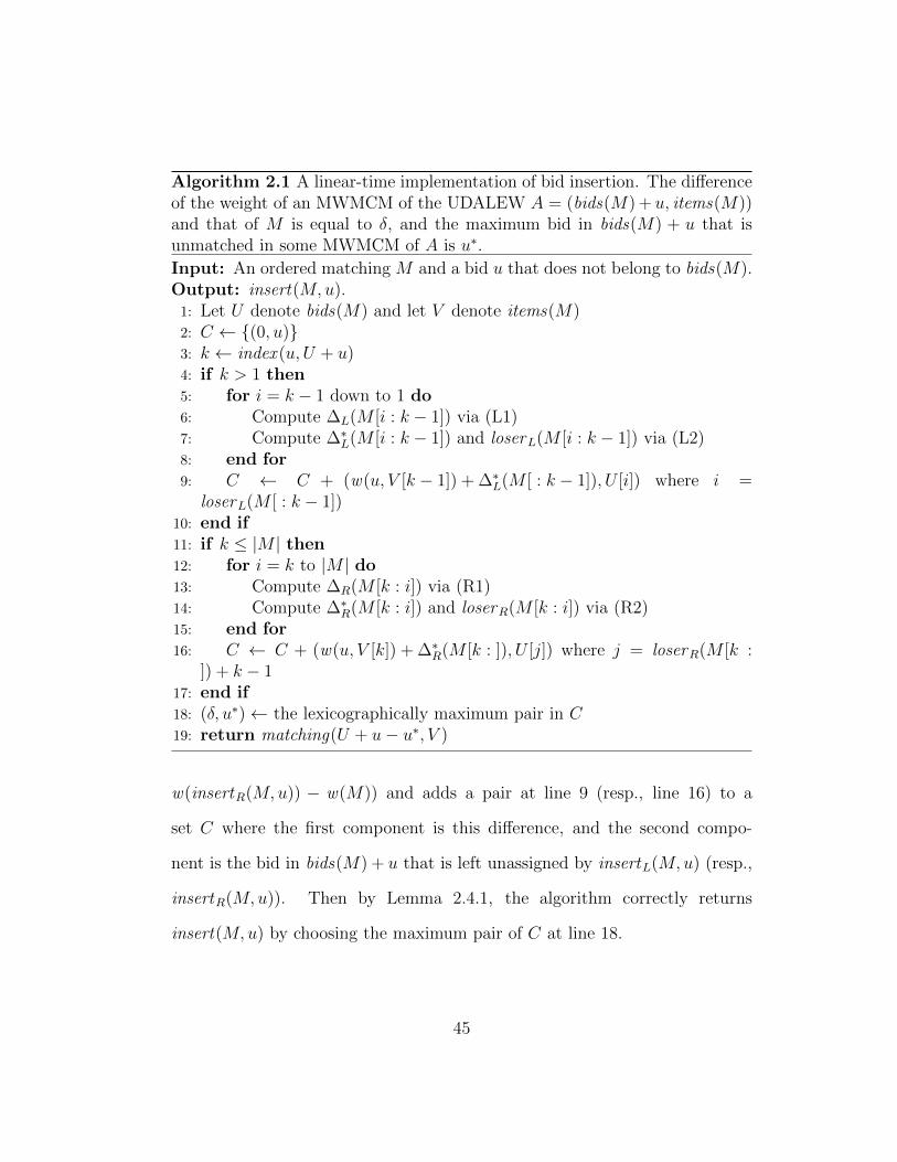
Algorithm 2.1 A linear-time implementation of bid insertion. The differenceof the weight of an MWMCM of the UDALEW A = (bids(M) + u, items(M))and that of M is equal to δ, and the maximum bid in bids(M) + u that isunmatched in some MWMCM of A is u∗.

Input: An ordered matching M and a bid u that does not belong to bids(M).Output: insert(M,u).

1: Let U denote bids(M) and let V denote items(M)2: C ← (0, u)3: k ← index (u, U + u)4: if k > 1 then5: for i = k − 1 down to 1 do6: Compute ∆L(M [i : k − 1]) via (L1)7: Compute ∆∗L(M [i : k − 1]) and loserL(M [i : k − 1]) via (L2)8: end for9: C ← C + (w(u, V [k − 1]) + ∆∗L(M [ : k − 1]), U [i]) where i =

loserL(M [ : k − 1])10: end if11: if k ≤ |M | then12: for i = k to |M | do13: Compute ∆R(M [k : i]) via (R1)14: Compute ∆∗R(M [k : i]) and loserR(M [k : i]) via (R2)15: end for16: C ← C + (w(u, V [k]) + ∆∗R(M [k : ]), U [j]) where j = loserR(M [k :

]) + k − 117: end if18: (δ, u∗)← the lexicographically maximum pair in C19: return matching(U + u− u∗, V )

w(insertR(M,u)) − w(M)) and adds a pair at line 9 (resp., line 16) to a

set C where the first component is this difference, and the second compo-

nent is the bid in bids(M) + u that is left unassigned by insertL(M,u) (resp.,

insertR(M,u)). Then by Lemma 2.4.1, the algorithm correctly returns

insert(M,u) by choosing the maximum pair of C at line 18.

45

2.5 A Superblock-Based Bid Insertion Algo-

rithm

In this section, we describe an ordered matching data structure based on the

concept of a “superblock”, and we show how to use this data structure to

obtain a significantly faster bid insertion algorithm than that presented in

Section 2.4. Before beginning our formal presentation in Section 2.5.1, we

provide a high-level overview of the main ideas. A reader interested in only

the formal presentation may proceed to Section 2.5.1 without loss of continuity.

Recall that an ordered matching data structure maintains a dynamic

ordered matching M . Let n denote |M |. We maintain a partition of the bids

of M into contiguous “groups” of size Θ(`), where ` is a parameter to be

optimized later. The time complexity of Algorithm 2.1 is linear because the

for loops starting at lines 5 and 12 process bid-item pairs in M sequentially.

Our rough plan is to accelerate the computations associated with this pair of

loops by proceeding group-by-group. We can process a group in constant time

if we are given six “auxiliary values” that depend on the “submatching” M ′ of

M associated with the bids in the group, namely: ∆L(M ′), ∆R(M ′), ∆∗L(M ′),

∆∗R(M ′), loserL(M ′), and loserR(M ′). The auxiliary values associated with a

group can be computed in Θ(`) time. A natural approach is to precompute

these auxiliary values when a group is created or modified, or when the set of

matched items associated with the group is modified. Unfortunately, a single

bid insertion can cause each bid in a contiguous interval of Θ(n) bids to have

46

a new matched item. For example, if a bid insertion introduces a “low” bid u

and deletes a “high” bid u′, then each bid between u and u′ gets a new matched

item one position to the right of its old matched item. Since a constant fraction

of the groups might need to have their auxiliary values recomputed as a result

of a bid insertion, the overall time complexity remains linear.

The preceding discussion suggests that it might be useful to have an

efficient way to obtain the new auxiliary values of a group of bids when the

corresponding interval of matched items is shifted left or right by one position.

To this end, we enhance the precomputation associated with a group of bids

as follows: Instead of precomputing only the auxiliary values corresponding

to the group’s current matched interval of items, we precompute the aux-

iliary values associated with shifts of 0,±1,±2, . . . ,±Θ(`) positions around

the current matched interval. That way, unless a group of bids is modified

(e.g., due to a bid being deleted or inserted) we do not need to redo the pre-

computation with the group until it has been shifted Ω(`) times. Since the

enhanced precomputation computes Θ(`) sets of auxiliary values instead of

one set, a naive implementation of the enhanced precomputation has Θ(`2)

time complexity, leading once again to linear worst-case time complexity for

bid insertion. We obtain a faster bid insertion algorithm by showing how to

perform the enhanced precomputation in O(` log2 `) time.

Our O(` log2 `)-time algorithm for performing the enhanced precom-

putation forms the core of our fast bid insertion algorithm. Here we briefly

mention the main techniques used to perform the enhanced precomputation

47

efficiently; the reader is referred to Section 2.6.1 for further details. A divide-

and-conquer approach is used to compute the auxiliary values associated with

the functions loserL and loserR in O(` log `) time; the correctness of this ap-

proach is based on a monotonicity result (see Lemmas2.6.3 and 2.6.4). A

convolution-based approach is used to compute the auxiliary values based on

∆L and ∆R in O(` log `) time (see Lemma 2.6.2). The auxiliary values based

on loserL (resp., loserR) are used within a divide-and-conquer framework to

compute the auxiliary values based on ∆∗L (resp., ∆∗R); in the associated re-

currence, the overhead term is dominated by the cost of evaluating the same

kind of convolution as in the computation of the auxiliary values based on ∆L

and ∆R. As a result, the overall time complexity for computing the auxiliary

values based on ∆∗L and ∆∗R is O(` log2 `).

Section 2.5.1 introduces the concept of a “block”, which is used to

represent a group of bids together with a contiguous interval of items that

includes all of the items matched to the group. Section 2.6.1 presents a block

data structure. When a block data structure is “initialized” with a group

of bids and an interval of items, the enhanced precomputation discussed in

the preceding paragraph is performed, and the associated auxiliary values are

stored in tables. A handful of “fields” associated with the block are also

initialized; these fields store basic information such as the number of bids

or items in the block. After initialization, the block data structure is read-

only: Whenever a block needs to be altered (e.g., because a bid needs to

be inserted/deleted, because the block needs to be merged with an adjacent

48

block), we destroy the block and create a new one. The operations supported

by a block may be partitioned into three categories: “queries”, “lookups” and

“scans”. Each query runs in constant time and returns the value of a specific

field. Each lookup runs in constant time and uses a table lookup to retrieve

one of the precomputed auxiliary values. Each of the two linear-time scan

operations (one leftgoing, one rightgoing) performs a naive emulation of one

of the for loops of Algorithm 2.1; in the context of a given bid insertion, such

operations are only invoked on the block containing the insertion position of

the new bid.

Section 2.5.1 defines the concept of a superblock, which is used to repre-

sent an ordered matching as a sequence of blocks. A superblock-based ordered

matching data structure is introduced in Section 2.6.2, where each of the con-

stituent blocks is represented using the block data structure alluded to in the

preceding paragraph. In Section 2.6, we simplify the presentation by setting

the parameter ` to Θ(√n). For this choice of `, we show that bid insertion can

be performed using O(1) block initializations, O(√n) block queries, O(

√n)

block lookups, at most two block scans, and O(√n) additional overhead, re-

sulting in an overall time complexity of O(√n log2 n). In terms of the param-

eters ` and n, the approach of Section 2.6 can be generalized to perform bid

insertion using O(dn/`2e) block initializations, O(n/`) block queries, O(n/`)

block lookups, at most two block scans, and O(n/`) additional overhead; it is

easy to verify that setting ` to Θ(√n) minimizes the overall time complexity.

49

2.5.1 Blocks and Superblocks

We define a block B as a UDALEW (U, V ) where |U | ≤ |V |. For any block

B = (U, V ), we define shifts(B) as |V | − |U | + 1. For any block B = (U, V )

and any integer t such that 1 ≤ t ≤ shifts(B), we define matching(B, t) as

matching(U, V [t : t+ |U | − 1]).

Let M be a nonempty ordered matching, let U denote bids(M), and

let V denote items(M). Let m be a positive integer, and let 〈a0, . . . , am〉,

〈b1, . . . , bm〉, and 〈c1, . . . , cm〉 be sequences of integers such that a0 = 0, am =

|U |, and 1 ≤ bi ≤ ai−1 + 1 ≤ ai ≤ ci ≤ |U | for 1 ≤ i ≤ m. Let Bi de-

note the block (U [ai−1 + 1 : ai], V [bi : ci]) for 1 ≤ i ≤ m. Then the list

of blocks S = 〈B1, . . . , Bm〉 is a superblock, and we make the following ad-

ditional definitions: matching(S) denotes M ; size(S) denotes |M |; bids(S)

denotes U ; items(S) denotes V ; shift(S, i) and shift(S,Bi) both denote bi −

ai−1 for 1 ≤ i ≤ m; sum(S, i) denotes ai for 0 ≤ i ≤ m; the leftmost

block B1 and the rightmost block Bm are the boundary blocks, the remain-

ing blocks B2, . . . , Bm−1 are the interior blocks. Remark: For any superblock

S, matching(S) =⋃

1≤i≤|S|matching(S[i], shift(S, i)).

2.5.2 Algorithm 2.2

We obtain a significantly faster bid insertion algorithm than Algorithm 2.1 by

accelerating the computations associated with the for loops starting at lines 5

and 12. Recall that the first loop computes ∆∗L(M [ : k − 1]) and loserL(M [ :

k − 1]), and the second one computes ∆∗R(M [k : ]) and loserR(M [k : ]). These

50

two loops process a trivial representation of M pair-by-pair using the recur-

rences (L1), (R1), (L2), and (R2). We start by generalizing these recurrences;

these generalizations allow us to compute the aforementioned values more ef-

ficiently by looping over a superblock-based representation of the matching

block-by-block, instead of pair-by-pair.

Let M denote matching(U, V ), and let i, j, and k be three indices in

M such that i ≤ j < k. Then the following equation generalizes (L1), and it

is straightforward to prove by repeated application of (L1).

∆L(M [i : k]) = ∆L(M [j + 1 : k]) + w(U [j + 1], V [j]) + ∆L(M [i : j]). (L1′)

We also give a generalization of (L2), where the proof follows from the defini-

tions of ∆∗L and loserL.

(∆∗L(M [i : k]), loserL(M [i : k])

)=

max

(∆∗L(M [j + 1 : k]), loserL(M [j + 1 : k]) + j + 1− i

),(

∆∗L(M [i : j]) + w(U [j + 1], V [j]) + ∆L(M [j + 1 : k]),

loserL(M [i : j]))

(L2′)

Let M denote matching(U, V ), and let i, j, and k be three indices in M

such that i < j ≤ k. Symmetrically, the following equations generalize (R1)

and (R2).

∆R(M [i : k]) = ∆R(M [i : j − 1]) + w(U [j − 1], V [j]) + ∆R(M [j : k]), (R1′)

51

and

(∆∗R(M [i : k]), loserR(M [i : k])

)=

max

(∆∗R(M [i : j − 1]), loserR(M [i : j − 1])

),(

∆∗R(M [j : k]) + w(U [j − 1], V [j]) + ∆R(M [i : j − 1]),

loserR(M [j : k]) + j − i)

(R2′)

We use (L1′) and (L2′) (resp., (R1′) and (R2′)) within a loop that iter-

ates over a superblock-based representation of the matching block-by-block. In

each iteration of the loop, we are able to evaluate the right-hand side of (L1′)

and (L2′) (resp., (R1′) and (R2′)) in constant time because the terms involving

M [j + 1 : k] (resp., M [i : j − 1]) are carried over from the previous iteration,

and the terms involving M [i : j] (resp., M [j : k]) are already stored in pre-

computed tables associated with the blocks of the superblock.

The high-level algorithm is given in Algorithm 2.2. The input is a su-

perblock S that represents an ordered matching, denoted M (i.e., matching(S)

= M), and a bid u that does not belong to bids(S). The output is a su-

perblock representing insert(M,u). The unique bid u∗ that is unmatched in

insert(M,u) is identified using the block-based framework alluded to above.

After identifying u∗, if u∗ 6= u, the algorithm invokes a subroutine Swap(S, u∗, u)

which, given a superblock S, a bid u∗ that belongs to bids(S), and a bid u that

does not belong to bids(S), returns a superblock that represents

matching(bids(S)+u−u∗, items(S)). We present our implementation of Swap

and analyze its time complexity in Sections 2.6.3 and 2.6.4. The correctness

52

Algorithm 2.2 A high-level bid insertion algorithm using the superblock-based representation of an ordered matching.

Input: A superblock S and a bid u that does not belong to bids(S).Output: A superblock S ′ such that matching(S ′) = insert(matching(S), u).

1: Let M denote matching(S), let U denote bids(S), and let V denoteitems(S)

2: Let S[i] be (Ui, Vi) for 1 ≤ i ≤ |S|3: σ(i)← sum(S, i) for 0 ≤ i ≤ |S|4: C ← (0, u)5: `← |(U ′, V ′) | (U ′, V ′) ∈ S and U ′[1] < u|6: k ← if ` < 1 then 1 else index (u, U` + u) + 1 + σ(`− 1)7: if k > 1 then8: for i = k − 1 down to σ(`− 1) + 1 do9: Compute ∆L(M [i : k − 1]) via (L1)

10: Compute ∆∗L(M [i : k − 1]) and loserL(M [i : k − 1]) via (L2)11: end for12: for i = `− 1 down to 1 do13: Compute ∆L(M [σ(i− 1) + 1 : k − 1]) via (L1′)14: Compute ∆∗L(M [σ(i− 1) + 1 : k − 1]) and loserL(M [σ(i− 1) + 1 :

k − 1]) via (L2′)15: end for16: C ← C + (w(u, V [k − 1]) + ∆∗L(M [ : k − 1]), U [i]) where i =

loserL(M [ : k − 1])17: end if18: if k ≤ |M | then19: for i = k to σ(`) do20: Compute ∆R(M [k : i]) via (R1)21: Compute ∆∗R(M [k : i]) and loserR(M [k : i]) via (R2)22: end for23: for i = `+ 1 to |S| do24: Compute ∆R(M [k : σ(i)]) via (R1′)25: Compute ∆∗R(M [k : σ(i)]) and loserR(M [k : σ(i)]) via (R2′)26: end for27: C ← C + (w(u, V [k]) + ∆∗R(M [k : ]), U [j]) where j = loserR(M [k :

]) + k − 128: end if29: (δ, u∗)← the lexicographically maximum pair in C30: return if u∗ 6= u then Swap(S, u∗, u) else S

53

of Algorithm 2.2 is established in Lemma 2.5.1, where it is shown that Algo-

rithm 2.2 emulates the behavior of Algorithm 2.1.

Lemma 2.5.1. Algorithm 2.2 is correct.

Proof. Assume that, given a superblock S, a bid u∗ that belongs to bids(S),

and a bid u that does not belong to bids(S), Swap(S, u∗, u) correctly returns

a superblock that represents matching(bids(S) + u − u∗, items(S)). Let M

denote matching(S), let U denote bids(S), and let V denote items(S), as in

the algorithm. First, the algorithm performs a scan over the blocks to compute

an integer ` at line 5 so that each bid in each block S[i] for 1 ≤ i < ` (resp., ` <

i ≤ |S|) is less (resp., greater) than the new bid u. Then it is easy to see that

the integer k computed at line 6 is equal to index (u, U+u), as in Algorithm 2.1.

It remains to show that ∆∗L(M [ : k − 1]), loserL(M [ : k − 1]), ∆∗R(M [k : ]),

and loserR(M [k : ]) are computed correctly so that the set C is populated

with the same pairs as in Algorithm 2.1, and thus Lemma 2.4.1 implies that

the bid u∗ in bids(M)+u that is left out by insert(M,u) is correctly identified

by choosing the maximum pair of C at line 29, as in Algorithm 2.1, and that

the superblock returned at line 30 represents insert(M,u).

If k > 1 (resp., k ≤ |M |), the algorithm proceeds to emulate the for

loop of Algorithm 2.1 that starts at line 5 (resp., line 12) to compute ∆∗L(M [ :

k − 1]) and loserL(M [ : k − 1]) (resp., ∆∗R(M [k : ]) and loserR(M [k : ])). We

first discuss the emulation of the loop of Algorithm 2.1 that starts at line 5; this

emulation is performed by two for loops in Algorithm 2.2. The first loop in Al-

gorithm 2.2, which starts at line 8, is identical to the loop of Algorithm 2.1, ex-

54

cept that it stops when the boundary of the submatching represented by block

S[`] is reached. Thus, by repeated application of (L1) and (L2), upon com-

pletion of this first loop, we have computed ∆L(M ′), ∆∗L(M ′), and loserL(M ′)

where M ′ denotes M [σ(`− 1) + 1 : k − 1]. Then the second for loop, which

starts at line 12, resumes where the first one left off; however, it utilizes the

superblock-based representation of the ordered matching to loop block-by-

block. During the iterations of the second loop, for i = `− 1 down to 1, (L1′)

and (L2′) are invoked by setting i, j, and k in these equations to σ(i− 1) + 1,

σ(i), and k − 1, respectively; thus the submatching M [i : j] in these equa-

tions corresponds to the submatching that the block S[i] represents in S, i.e.,

matching(S[i], shift(S, i)). During such an iteration i, for i = ` − 1 down to

1, the terms involving M [i : j] in (L1′) and (L2′), i.e., the terms that are

equal to ∆L(matching(S[i], shift(S, i))), ∆∗L(matching(S[i], shift(S, i))), and

loserL(matching(S[i], shift(S, i))), are fetched from the precomputed tables

associated with the block S[i]. Note that all the terms in these equations in-

volving M [j + 1 : k] are carried over from the previous iteration, except for the

first iteration, where they are already computed by the first for loop. Thus,

upon completion of these two loops, we have computed ∆∗L(M [ : k − 1]) and

loserL(M [ : k − 1]).

The emulation of the second loop of Algorithm 2.1 (starting at line 12)

that computes ∆∗R(M [k : ]) and loserR(M [k : ]) can be argued symmetrically,

where (R1′) and (R2′) are invoked in the for loop at line 23 by setting i, j,

and k in these equations to k, σ(i − 1) + 1, and σ(i), respectively. Then the

55

submatching M [j : k] in these equations corresponds to the submatching that

the block S[i] represents in S, i.e., matching(S[i], shift(S, i)).

2.6 Fast Implementation of Algorithm 2.2

In this section, we complete the discussion of our fast bid insertion algorithm by

describing two data structures, giving the implementation details, and analyz-

ing the running time. First, in Section 2.6.1, we present a block data structure

that precomputes the auxiliary tables mentioned in Section 2.5.2 in quasilinear

time, thus allowing lines 13, 14, 24, and 25 of Algorithm 2.2 to be performed

in constant time. Then, in Section 2.6.2, we introduce a superblock-based

ordered matching data structure that stores the blocks using the block data

structure, where the sizes of the blocks are optimized to balance the cost of

Swap with that of the remaining operations in Algorithm 2.2. Finally, in Sec-

tions 2.6.3 and 2.6.4, we present our efficient implementation of Swap, which

constructs only a constant number of blocks, and analyze its time complexity.

2.6.1 Block Data Structure

Let S be a superblock on which a bid insertion is performed, let B be a

block in S, and let Mt denote matching(B, t) for 1 ≤ t ≤ shifts(B). The

algorithm may query ∆L(Mt), ∆R(Mt), ∆∗L(Mt), ∆∗R(Mt), loserL(Mt), and

loserR(Mt) for t = shift(S,B). If B is part of the superblocks for a series

of bid insertions, then these queries may be performed for various t values.

56

For a fast implementation of Algorithm 2.2, instead of individually computing

these quantities at query time, we efficiently precompute them during the

construction of the block and store them in the following six lists. We define

∆L(B) as the list of size shifts(B) such that ∆L(B)[t] is equal to ∆L(Mt) for

1 ≤ t ≤ shifts(B). We define the lists ∆R(B), ∆∗L(B), ∆∗R(B), loserL(B),

and loserR(B) similarly. The representation of a block B = (U, V ) simply

maintains each of the following explicitly as an array: U , V , ∆L(B), ∆R(B),

∆∗L(B), ∆∗R(B), loserL(B), and loserR(B). In what follows, we refer to that

representation as the block data structure for B. The block data structure

is an integral part of the superblock-based ordered matching data structure

which we introduce in the following section.

Theorem 2.6.1. Let B be a block (U, V ). Then the block data structure for

B can be constructed in O(|V | (log shifts(B) + log2 |U |)) time.

The proof of Theorem 2.6.1 follows directly from Lemmas 2.6.2, 2.6.5,

and 2.6.6 below.

Lemma 2.6.2. Let B be a block (U, V ). Then ∆L(B) and ∆R(B) can be

computed in O(|V | log |U |) time.

Proof. We address the computation of ∆L(B), the computation of ∆R(B)

is symmetric. Let β denote ∆L(B). We define the following two real-valued

functions on the set of integers. Let x(n) be V [n+1].quality−V [n+2].quality ,

if 0 ≤ n < |V |−1; 0, otherwise. Let h(n) be U [|U |−n].slope, if 0 ≤ n < |U |−1;

0, otherwise. Let y(n) denote the discrete convolution (x ∗h)(n) =∑

m h(m) ·

57

x(n−m). Then, for 1 ≤ t ≤ shifts(B),

β[t] =∑

1<i≤|U |

w(U [i], V [i+ t− 2])−∑

1≤i≤|U |

w(U [i], V [i+ t− 1])

= −w(U [1], V [t]) +∑1<i≤|U |

U [i].slope · (V [i+ t− 2].quality − V [i+ t− 1].quality)

= −w(U [1], V [t]) +∑

1<i≤|U |

h(|U | − i) · x(i+ t− 3)

= −w(U [1], V [t]) +∑

0≤m<|U |−1

h(m) · x(|U | −m+ t− 3)

= −w(U [1], V [t]) + y(t+ |U | − 3),

where the convolution y(n) = (x∗h)(n) can be computed in O(|V | log |U |) time

by computing Θ(|U |)-size segments of y(n) using fast circular convolution, and

concatenating the segments together [47].

The next two lemmas establish a monotonicity result that is used to

prove Lemma 2.6.5.

Lemma 2.6.3. Let B be a block (U, V ) and let α denote loserL(B). Then for

any integer t such that 1 ≤ t < shifts(B), α[t] ≥ α[t+ 1].

Proof. For the sake of contradiction, suppose α[t] < α[t + 1] for some t such

that 1 ≤ t < shifts(B). Let M denote matching(B, t) and let M ′ denote

matching(B, t+ 1). Let i denote α[t] = loserL(M) and let i′ denote α[t+ 1] =

loserL(M ′). Since i = loserL(M) < i′, we have ∆L(M [i : ]) > ∆L(M [i′ : ]),

58

which, together with (L1′), implies ∆L(M [i : i′]) > ∆L(M [i′]), and hence

∑i<`≤i′

w(U [`], V [`+ t− 2])−∑i≤`<i′

w(U [`], V [`+ t− 1]) > 0. (2.1)

Since i′ = loserL(M ′), we have ∆L(M ′[i : ]) ≤ ∆L(M ′[i′ : ]), which, together

with (L1′), implies ∆L(M ′[i : i′]) ≤ ∆L(M ′[i′]), and hence

∑i<`≤i′

w(U [`], V [`+ t− 1])−∑i≤`<i′

w(U [`], V [`+ t]) ≤ 0. (2.2)

Subtracting (2.1) from (2.2), we get

0 >∑i<`≤i′

[w(U [`], V [`+ t− 1])− w(U [`], V [`+ t− 2])]

−∑i≤`<i′

[w(U [`], V [`+ t])− w(U [`], V [`+ t− 1])]

=∑i≤`<i′

U [`+ 1].slope · (V [`+ t].quality − V [`+ t− 1].quality)

−∑i≤`<i′

U [`].slope · (V [`+ t].quality − V [`+ t− 1].quality)

=∑i≤`<i′

(U [`+ 1].slope − U [`].slope)(V [`+ t].quality − V [`+ t− 1].quality),

which contradicts the way that the bids in U and the items in V are ordered.

Lemma 2.6.4. Let B be a block (U, V ) and let α denote loserR(B). Then

for any integer t such that 1 ≤ t < shifts(B), α[t] ≤ α[t+ 1].

59

Proof. Symmetric to the proof of Lemma 2.6.3.

We now introduce two definitions that return “subblocks” of a block

and that are useful in the proofs of Lemmas 2.6.5 and 2.6.6 which give divide-

and-conquer algorithms.

For any block B = (U, V ) and for any two indices i and i′ such that 1 ≤

i ≤ i′ ≤ |U |, we define subBids(B, i, i′) as the block B′ such that shifts(B′) =

shifts(B) and matching(B′, t) = Mt[i : i′] for 1 ≤ t ≤ shifts(B), where Mt

denotes matching(B, t); it is straightforward to see that subBids(B, i, i′) =

(U [i : i′], V [i : |V | − |U |+ i′]).

For any block B = (U, V ) and for any two integers t and t′ such that

1 ≤ t ≤ t′ ≤ shifts(B), we define subShifts(B, t, t′) as the block B′ such

that shifts(B′) = t′ − t + 1 and matching(B′, t′′) = matching(B, t′′ + t − 1)

for 1 ≤ t′′ ≤ shifts(B′); it is straightforward to see that subShifts(B, t, t′) =

(U, V [t : |V | − shifts(B) + t′]).

Lemma 2.6.5. Let B be a block (U, V ). Then loserL(B) and loserR(B) can

be computed in O(|V | log shifts(B)) time.

Proof. We address the computation of loserL(B), which relies on Lemma 2.6.3.

The computation of loserR(B) is symmetric, and relies on Lemma 2.6.4. We

begin by stating a useful claim.

Let M be an ordered matching and let j be an index in M . Then we

claim that, loserL(M) ≤ j implies loserL(M) = loserL(M [ : j]); similarly,

loserL(M) ≥ j implies loserL(M) = loserL(M [j : ]) + j − 1. The proof of the

claim is immediate from (L2′).

60

Let α denote loserL(B). We give a divide-and-conquer algorithm that

computes α. If |U | = 1, then α[t] = 1 for any t and we are done; otherwise,

we proceed as follows. Let t∗ denote dshifts(B)/2e and let m denote α[t∗].

We first compute m in O(|U |) time using (L1) and (L2). Let B1 denote the

block subBids(B, 1,m) and let B2 denote the block subBids(B,m, |U |). Let

α1 denote loserL(B1) and let α2 denote loserL(B2). Then, by Lemma 2.6.3

and by the claim of the preceding paragraph,

α[t] =

α1[t] if t∗ < t ≤ shifts(B)

m if t = t∗

α2[t] +m− 1 if 1 ≤ t < t∗.

Thus, it remains to compute α1[t∗ + 1 : shifts(B)] and α2[1 : t∗ − 1]. Note that

α1[t∗ + 1 : shifts(B)] is equal to loserL(B′1) for the blockB′1 = subShifts(B1, t

∗+

1, shifts(B)), so we compute it recursively. Similarly, α2[1 : t∗ − 1] is equal to

loserL(B′2) for the block B′2 = subShifts(B2, 1, t∗− 1), so we compute it recur-

sively.

The overall running time satisfies the recurrence

T (n, s) ≤ T (m, s/2) + T (n−m+ 1, s/2) +O(n+ s),

where n denotes |U | and s denotes shifts(B) for the input block B = (U, V ).

Solving this recurrence, we obtain the desired running time.

Lemma 2.6.6. Let B be a block (U, V ). Then ∆∗L(B) can be computed

61

in O(|V | log2 |U |) time given loserL(B). Similarly, ∆∗R(B) can be computed

within the same time bound given loserR(B).

Proof. We address the computation of ∆∗L(B), which relies on Lemma 2.6.3.

The computation of ∆∗R(B) is symmetric, and relies on Lemma 2.6.4.

Let α denote loserL(B) and let β∗ denote ∆∗L(B). We now give a divide-

and-conquer algorithm that computes β∗. If |U | ≤ 2, then β∗ can be computed

trivially in O(shifts(B)) time; otherwise, we proceed as follows. Let m denote

d|U | /2e. Let B1 denote the block subBids(B, 1,m) and let B2 denote the block

subBids(B,m + 1, |U |). Let α1 denote loserL(B1) and let β∗1 denote ∆∗L(B1).

Let α2 denote loserL(B2), let β∗2 denote ∆∗L(B2), and let β2 denote ∆L(B2).

Lemma 2.6.3 and the claim in the beginning of the proof of Lemma 2.6.5 imply

that there exists an integer t′ such that 0 ≤ t′ ≤ shifts(B), α[t] = α1[t] for

t′ < t ≤ shifts(B), and α[t] = α2[t] +m− 1 for 1 ≤ t ≤ t′; in what follows let

t∗ denote the largest such integer. Then, by (L2′),

β∗[t] =

β∗1 [t] + β2[t] + w(U [m+ 1], V [m+ t− 1]) if t∗ < t ≤ shifts(B)

β∗2 [t] if 1 ≤ t ≤ t∗.

Thus, it remains to compute β∗1 [t∗ + 1 : shifts(B)], β∗2 [1 : t∗], and β2[t∗ + 1 :

shifts(B)]. Note that β∗1 [t∗ + 1 : shifts(B)] is equal to ∆∗L(B′1) for the block

B′1 = subShifts(B1, t∗ + 1, shifts(B)), so we compute it recursively. Similarly,

β∗2 [1 : t∗] is equal to ∆∗L(B′2) for the block B′2 = subShifts(B2, 1, t∗), so we

compute it recursively. Finally, β2[t∗ + 1 : shifts(B)] is equal to ∆L(B′′2 ) for the

block B′′2 = subShifts(B2, t∗+1, shifts(B)), and we compute it in O(|V | log |U |)

62

time by Lemma 2.6.2.

The overall running time satisfies the recurrence

T (n, s) ≤ T (n/2, t) + T (n/2, s− t) +O((n+ s) log n),

where n denotes |U | and s denotes shifts(B) for the input block B = (U, V ).

Solving this recurrence, we obtain the desired running time.

2.6.2 Superblock-Based Ordered Matching

In this section, we introduce a data structure called a superblock-based ordered

matching (SOM ). A SOM represents an ordered matching M by maintaining

a superblock S such that matching(S) = M , where S is stored as a list of

block data structures as described in Section 2.6.1.

Theorem 2.6.7. The SOM has initialization cost O(n log2 n), bid insertion

cost O(√n log2 n), and dump cost O(n).

Theorem 2.6.7 states our main result, and is proved in Section 2.6.4.

We first briefly mention key performance-related properties of the SOM that

are used for our efficient implementation of Algorithm 2.2. Throughout the

rest of this paragraph, let n denote the size of the matching represented by the

SOM. We group the operations performed during Algorithm 2.2 into three cat-

egories: ∆L(M ′′), ∆R(M ′′), ∆∗L(M ′′), ∆∗R(M ′′), loserL(M ′′), and loserR(M ′′)

queries for submatchings M ′′ of M ; the remaining operations performed in

lines 1 through 29; the Swap operation. It is easy to see that Algorithm 2.2

63

does not modify the superblock, except during Swap at line 30. When Swap

modifies the superblock, existing blocks are not modified; rather, some existing

blocks are deleted, and some newly constructed blocks are inserted. Since the

SOM stores the superblock as a list of block data structures as described in Sec-

tion 2.6.1, all the values in the auxiliary tables ∆L(B), ∆R(B), ∆∗L(B), ∆∗R(B),

loserL(B), and loserR(B) are available for each block B. Thus, the queries

for ∆L(M ′′), ∆R(M ′′), ∆∗L(M ′′), ∆∗R(M ′′), loserL(M ′′), and loserR(M ′′) for

each 1 ≤ i ≤ |S| can be answered in constant time, where M ′′ denotes

matching(S[i], shift(S, i)). It is easy to see by inspecting the code of Algo-

rithm 2.2 that the number of such queries is proportional to the number of

blocks in the superblock. Furthermore, the running time of all the remaining

operations performed in lines 1 through 29 is proportional to the maximum of

(1) the number of blocks in the superblock, and (2) the maximum number of

bids in any single block. We define the blocks in a SOM so that each block

has Θ(√n) bids and Θ(

√n) items, yielding a Θ(

√n)-time implementation of

lines 1 through 29, and so that Swap can be implemented by constructing at

most a constant number of blocks. Later in this section, we formally define the

SOM, and we introduce two invariants that are related to these requirements.

Then in Sections 2.6.3 and 2.6.4, we present a detailed O(√n log2 n)-time im-

plementation of Swap for the SOM that constructs at most a constant number

of blocks. We begin with some useful definitions.

For any non-empty ordered matching M , we define slice(M) as d√ne

where n denotes |M |, and we find it convenient to overload slice so that slice(S)

64

denotes slice(matching(S)).

Let S be a superblock and let B be a block that belongs to S. Then we

define time(S,B) as min(shift(S,B), shifts(B)−shift(S,B)+1). Observe that

matching(B, t) is well-defined for all t such that shift(S,B)− time(S,B) < t <

shift(S,B) + time(S,B).

We now introduce two invariants that we maintain regarding

the performance-related concerns mentioned above. The first invariant ensures

that the number of bids in each block is at least√n and less than 2 d

√ne, thus

there are at most√n blocks, where n denotes size(S). The second invariant

ensures that there are not too many blocks B in the superblock S whose time

time(S,B) is low, thus Swap does not require more than a constant number

of block constructions. We now formally define these two invariants.

For any superblock S, we define the predicate P(S) to hold if for each

block (U, V ) in S, slice(S) ≤ |U | < 2 · slice(S).

For any superblock S, we define the predicate Q(S) to hold if for any

` such that 1 ≤ ` ≤ slice(S), there are at most ` interior blocks B of S such

that time(S,B) ≤ `.

We say that a superblock S is nice if P(S) ∧Q(S).

We say that an ordered matching data structure D is a superblock-based

ordered matching (SOM ) if it represents an ordered matching M by maintain-

ing a nice superblock S such that matching(S) = M , and the superblock S

is stored as a list of block data structures that are described earlier in Sec-

tion 2.6.1.

65

2.6.3 Block-Level Operations

Having defined the SOM, it remains to show how to implement Swap effi-

ciently on the SOM. We describe Swap by means of four kinds of block-level

operations: refresh, split , merge, and exchange. As stated earlier, the primary

goal of Swap is to update the matching, and exchange establishes that. The

other three operations, refresh, split , and merge, do not alter the matching;

the purpose of these operations is to maintain the two invariants defined in

Section 2.6.2. The common goal of the split and merge operations is to keep

the number of bids in each block of a superblock S within a constant factor

of slice(S), and to keep |S| at most slice(S). In addition, for any block B

that is created by any of these four block-level operations on a superblock S,

shifts(B) is within a constant factor of slice(S). We define here what each of

these operations establishes and we outline how these operations are chained

together in order to achieve a Swap implementation, we defer the analysis of

the running times to Section 2.6.4. We start with some useful definitions.

All of the four block-level operations operate by replacing one or two

existing blocks with one or two new blocks. We now outline how the new

blocks are chosen by these operations. The choice of the bid set of a new block

directly depends on the type of the operation: it is equal to the bid set of the

block to be replaced by a refresh, or it is one of the two halves of the bid set

of the block to be replaced by a split , or it is the union of the bid sets of the

two blocks to be replaced by a merge, or one bid is removed and/or one bid is

added to the bid set of a block to be replaced by a exchange. The exact details

66

are given in the paragraphs below that introduce the individual operations.

Given the bid set of the block that is to be created, the choice of the item set

of the block depends only on the matching that the superblock resulting from

the operation represents. Thus, any new block that the block-level operations

create can be expressed as a function of the resulting matching M and the

set U of the bids that are involved in the block. This function fresh(M,U) is

defined as follows.

Let M be an ordered matching and let U be a contiguous subset of

bids(M). Let i denote index (U [1], bids(M)) and let V denote items(M). Let

U≺ denote the set u′ | u′ ∈ bids(M) ∧ u′ U [|U |] (note that |U≺| = i−1 and |U| = |M |−|U |−

|U≺|). Then, we define fresh(M,U) as the block (U, V [i− r : i+ |U | − 1 + r])

where r denotes 2 ·min(slice(M), |U≺| , |U|). For any superblock S and any

block B in S that is equal to fresh(matching(S), U) for some U , we make

the following two observations: (1) time(S,B) = maxS′ time(S ′, B) where the

maximum is taken over all possible superblocks that B can be a part of; (2)

time(S,B) = 1 + slice(S) unless the degenerate condition min(|U≺| , |U|) <

slice(S) holds, where U≺ and U are defined as earlier in this paragraph. It

will be explained later that, at the end of each bid insertion, the degenerate

condition mentioned in the preceding observation only holds for the boundary

blocks.

We are now ready to introduce the four block-level operations that the

SOM performs to modify the superblock that it maintains. In order to define

67

what these operations establish, we introduce a function for each operation

that takes a superblock as input (with additional arguments for exchange)

and returns another one.

For any superblock S, we define refresh(S) as the superblock that is

identical to S except that, if it exists, the block B = (U, V ) among all interior

blocks with the lowest time(S,B), breaking ties by choosing the block with

the lowest index, is replaced with fresh(matching(S), U).

For any superblock S, we define split(S) as the superblock that is iden-

tical to S except that, if it exists, the block B = (U, V ) with the lowest

index among the ones satisfying |U | ≥ 2 · slice(S) is replaced with two blocks

fresh(matching(S), U [ : m]) and fresh(matching(S), U [m+ 1 : ]), where m

denotes d|U | /2e.

For any superblock S, we define merge(S) as the superblock that is

identical to S except that, if it exists, the block B = (U, V ) with the lowest

index among the ones satisfying |U | < slice(S), and the block B′ = (U ′, V ′)

with the lowest index among the at most two that are adjacent to B, are

replaced with a single block fresh(matching(S), U ∪ U ′).

It is easy to see that matching(refresh(S)), matching(split(S)), and

matching(merge(S)) are all equal to matching(S). However, the following

function returns a superblock that represents a matching that is different than

the one its input represents, by exchanging an existing bid for a new bid.

Let S be a superblock such that time(S,B) > 1 for each interior block

B in S, let u∗ be a bid that belongs to bids(S), let u be a bid that does not be-

68

long to bids(S), and let M denote matching(bids(S)−u∗+u, items(S)). Then

we define exchange(S, u∗, u), which returns a superblock that represents M

and that is identical to S with the exception of at most two blocks, as follows:

let B∗ = (U∗, V ∗) denote the block in S that contains u∗; let B† = (U †, V †)

denote the block with the lowest index among the ones in S satisfying that

U †+u is a contiguous subset of bids(S)+u; if B∗ = B†, then exchange(S, u∗, u)

is identical to S except that B∗ is replaced with fresh(M,U∗ − u∗ + u), oth-

erwise, exchange(S, u∗, u) is identical to S except that B∗ is replaced with

fresh(M,U∗ − u∗) and B† is replaced with fresh(M,U † + u).

In order to justify that exchange(S, u∗, u) returns a valid superblock

that represents the desired matching, we now compare matching(S) with the

desired matching from the perspectives of bids and blocks. In what follows, let

S be a superblock and let u∗ and u be two bids such that exchange(S, u∗, u)

is well-defined, and let S ′ denote exchange(S, u∗, u). Let U denote bids(S), let

V denote items(S), let M denote matching(S), and let M ′ denote the desired

matching matching(U−u∗+u, V ). Let k∗ denote index (u∗, U) and let k denote

index (u, U+u). Let B∗ and B† be the blocks defined as in the preceding para-

graph, let `∗ denote index (B∗, S), and let `† denote index (B†, S). Comparing

M with M ′ from the perspective of bids, it is straightforward to see that, if

k∗ < k (resp., k∗ ≥ k) then u is assigned to V [k − 1] (resp., V [k]) in M ′, and

for each i such that k∗ < i ≤ k − 1 (resp., k ≤ i < k∗), the bid U [i], which is

assigned to V [i] in M , is shifted left (resp., right) by exchange(S, u∗, u), i.e., is

assigned to V [i−1] (resp., V [i+1]) in M ′. Each bid that belongs to U but that

69

is neither shifted left nor right by exchange(S, u∗, u) is assigned to the same

item in both M and M ′, except for u∗ which is unassigned in M ′. Comparing

M with M ′ from the perspective of the blocks, it is easy to see that, if `∗ < `†

(resp., `∗ > `†), then each bid in each block S[i] with a block index `∗ i > `†) is shifted left (resp., right), hence, we say that the block

S[i] is shifted left (resp., right) by exchange(S, u∗, u). For each block B that is

shifted left (resp., right) by exchange(S, u∗, u), shift(S ′, B) = shift(S,B) − 1

(resp., +1), and for each block B that belongs to both S and S ′ but that is

neither shifted left nor right, shift(S ′, B) = shift(S,B). Thus, since B∗ and B†

are replaced with new blocks in S ′ and since time(S,B) > 1 for each interior

block B that belongs to S, matching(B, shift(S ′, B)) is well-defined for each

block B that belongs to S ′. Hence, S ′ is a valid superblock and it is easy to

see that matching(S ′) = M ′.

We now define a function via refresh, exchange, split , and merge that

proves to be useful in our goal of efficiently implementing Swap on the SOM.

For any nice superblock S, any bid u∗ that belongs to bids(S), and any

bid u that does not belong to bids(S), we define swap(S, u∗, u) as

split(merge(split(exchange(refresh(S), u∗, u)))).

The following lemma suggests using S = swap(S, u∗, u) as an implementation

of Swap(S, u∗, u) since it modifies the superblock as desired while maintaining

the predicates P(S) and Q(S).

Lemma 2.6.8. Let S be a nice superblock, let u∗ be a bid that belongs to

70

bids(S), and let u be a bid that does not belong to bids(S). Then swap(S, u∗, u)

is a nice superblock, and matching(swap(S, u∗, u)) = matching(bids(S) + u−

u∗, items(S)).

Proof. Let S1 denote refresh(S). By the definition of refresh, matching(S1) =

matching(S). Since S is nice, P(S) and Q(S) holds. Then, since refresh does

not change the bid partitioning implied by the superblock, P(S1) holds. And

since refresh only replaces an interior block B with the lowest time(S,B), if it

exists, with a block B′ having time(S1, B′) = slice(S1)+1, it is straightforward

to see that a stronger Q(S1) (thus implying Q(S1)) holds, which we define next

as Q+(S1).

For any superblock S, we define the predicate Q+(S) to hold if for any

` such that 1 ≤ ` ≤ slice(S), there are at most ` − 1 interior blocks B of S

such that time(S,B) ≤ `.

Let S2 denote exchange(S1, u∗, u). Since Q+(S1) implies that time(S1, B)

is greater than 1 for each interior block B in S1, exchange(S1, u∗, u) is well-

defined, and hence matching(S2) = matching(bids(S) + u − u∗, items(S)).

Now, if only one block is replaced during exchange(S1, u∗, u), then the follow-

ing claims hold: P(S2) since the replaced block has the same number of bids;

Q+(S2), and thus Q(S2) since no blocks are shifted; hence, split(merge(split(S2)))

is equal to S2, which is a nice superblock with the desired matching, and we

are done. If two blocks are replaced, then it is straightforward to see that

the following claims hold by the definition of exchange: Q(S2) since Q+(S1)

and the fact that |shift(S2, B)− shift(S1, B)| ≤ 1 for each surviving block B,

71

where the latter fact is a result of the shifts, as described while arguing the

correctness of exchange; P(S2) except that one block may be undersized by

one bid and one block may be oversized by one bid.

Let S3 denote split(S2). It is straightforward to see that the following

claims hold by the definition of split : matching(S3) = matching(S2); Q(S3);

P(S3) except that one block may be undersized by one bid.

Let S4 denote merge(S3). It is straightforward to see that the following

claims hold by the definition of merge: matching(S4) = matching(S3); Q(S4);

P(S4) except that one block may be oversized with total number of bids at

most 3 · slice(S)− 2.

Let S5 denote split(S4). It is straightforward to see that the following

claims hold by the definition of split : matching(S5) = matching(S4); Q(S5);

P(S5).

By the preceding observations, we see that S5, which is equal to

swap(S, u∗, u), is a nice superblock and matching(S5) = matching(S2) =

matching(bids(S) + u− u∗, items(S)), as required.

2.6.4 Implementation of Swap and Time Complexity

We now complete the discussion of the fast bid insertion on the SOM by de-

scribing how to efficiently implement Swap as S = swap(S, u∗, u), as described

in the preceding section, and by proving Theorem 2.6.7, which summarizes our

results. Recall that the goal of Swap(S, u∗, u) is, given a superblock S, a bid

u∗ that belongs to bids(S), and a bid u that does not belong to bids(S), to

72

return a superblock that represents matching(bids(S)+u−u∗, items(S)); since

a SOM always maintains a nice superblock, we require the input S and the

returned superblock to be nice.

Lemma 2.6.9. Let D be a SOM, let S denote the superblock maintained by

D, and let n denote size(S). Then, Swap(S, u∗, u) on D can be implemented

as S = swap(S, u∗, u) in O(√n log2 n) time.

Proof. Lemma 2.6.8 implies that S = swap(S, u∗, u) is a correct implemen-

tation of Swap(S, u∗, u), and it satisfies the requirement that D maintains a

nice superblock. We now argue the running time. It is straightforward to see

that each of the operations refresh, exchange, split , and merge can be imple-

mented in O(√n log2 n) time; it takes O(|S|) = O(

√n) time to identify the

block/blocks to be replaced, since P(S) implies that |S| is Θ(√n); it takes

O(√n log2 n) time to construct each block B = (U, V ) by Theorem 2.6.1, since

P(S) and the definition of fresh implies that |U |, |V |, and shifts(B) are O(√n);

there are at most two block constructions per operation.

Proof of Theorem 2.6.7. When initialized with an ordered matching M with

size n, the SOM constructs Θ(√n) blocks, each taking O(

√n log2 n) time.

Bid insertion on the SOM can be implemented as Algorithm 2.2 in

O(√n log2 n) time since Lemma 2.6.9 shows that Swap(S, u∗, u) can be im-

plemented in O(√n log2 n) time, and as argued in Section 2.6.2, the remaining

operations in Algorithm 2.2 can be implemented in O(√n) time, where n

denotes the size of the superblock that the SOM maintains.

73

It is straightforward to implement dump by scanning over all the blocks

and constructing a list representation of the matching in O(n) time where n

denotes the size of the matching.

2.7 Computation of the VCG Prices

In this section, we show how to extend the SOM to maintain the VCG prices

as each bid is inserted. Section 2.7.1 introduces some useful definitions. Sec-

tion 2.7.2 extends the incremental framework of Section 2.3 to compute the

VCG prices. Section 2.7.3 presents a basic algorithm within the framework

of Section 2.7.2. Section 2.7.6 describes how to extend the data structure of

Section 2.5 and presents a fast emulation of the algorithm of Section 2.7.3.

2.7.1 Preliminaries

We begin by reviewing some standard definitions and results that prove to be

useful. We state these results for UDALEWs; however, they hold for general

unit-demand auctions. (The reader is referred to [51, Chapter 8] for a thorough

discussion and omitted proofs.)

For a UDALEW A = (U, V ), a surplus vector s assigns a real value s [i]

to each bid U [i] in U , a price vector p assigns a real value p[j] to each item

V [j] in V , and an outcome is a triple (M, s , p) such that s is a surplus vector,

p is a price vector, and M is a matching of A.

An outcome (M, s , p) of a UDALEW (U, V ) is feasible if∑

1≤i≤|U | s [i]+

74

∑1≤j≤|V | p[j] = w(M). For any feasible outcome (M, s , p), we say that the

pair of vectors (s , p) and the matching M are compatible.

Let A = (U, V ) be a UDALEW. We say that a bid U [i] (resp., item

V [j]) blocks an outcome (M, s , p) of A if s [i] < 0 (resp., p[j] < 0). We say

that a bid-item pair (U [i], V [j]) blocks an outcome (M, s , p) of A if s [i]+p[j] <

w(U [i], V [j]). If no bid, item, or bid-item pair blocks an outcome (M, s , p) of A

, then we say that the outcome (M, s , p) is stable, and that the payoff (s , p) is

stable with M . For any stable outcome (M, s , p) of A, the following are known:

M is an MWM of A; s [i] + p[j] = w(U [i], V [j]) for all (U [i], V [j]) matched in

M ; s [i] = 0 for all U [i] unmatched in M ; p[j] = 0 for all V [j] unmatched in M .

It is also known that any MWM is compatible with any stable payoff. Thus,

given the price vector p of a stable outcome of A, the corresponding surplus

vector s is uniquely determined by the following equation, where M denotes

an arbitrary MWM of A:

s [i] =

w(U [i], V [j])− p[j] if V [j] is assigned to U [i] in M

0 if U [i] is left unassigned in M.

(2.3)

For any stable payoff (s , p) of A, we say that p is a stable price vector of A.

In the remainder of Section 2.7, we write an outcome as a pair (M, p)

rather than a triple (M, s , p), and it is understood that the associated surplus

vector s is given by (2.3).

It is known that the stable price vectors of a UDALEW form a lat-

tice [55]. Hence, there is a unique stable price vector that is componentwise

75

less than or equal to any other stable price vector; this minimum stable price

vector corresponds to the VCG prices [40]. Thus, for a UDALEW A, we refer

to a stable outcome (M, p) of A as a VCG outcome of A if p is the VCG prices.

In the remainder of Section 2.7, the inequality operators denote componentwise

inequalities when they are used on price vectors.

2.7.2 Incremental Framework with Prices

In this section, we present an incremental framework for the problem of finding

a VCG outcome of a UDALEW; we follow the approach of Section 2.3. In order

to utilize the algorithms of Sections 2.4 and 2.5, we assume that the UDALEW

(U, V ) for which we seek a VCG outcome is enlarged by adding |V | dummy

bids, each with intercept zero and slope zero, so that, by Corollary 2.3.2, we

can restrict our attention to ordered MWMCMs. Hence, in the remainder of

Section 2.7, for any outcome (M, p) of a UDALEW A, we impose the condition

that M is an ordered MWMCM of A.

Let A = (U, V ) be a UDALEW such that |U | ≥ |V |. Then for any

VCG outcome (M, p) of A and any bid u that does not belong to U , we

define insert(M, p, u) as the stable outcome (M ′, p ′) of the UDALEW A′ =

(bids(M) + u, items(M)) where M ′ is insert(M,u) and p ′ is the minimum

stable price vector of A′ such that p ′ ≥ p; the existence and uniqueness of

such p ′ is implied by the lattice property of the stable price vectors.

The following lemma is at the core of our incremental framework. The

proof follows from [51, Proposition 8.17] and from Lemma 2.3.3.

76

Lemma 2.7.1. Let A = (U, V ) be a UDALEW such that |U | ≥ |V | and let u

be a bid that does not belong to U . Then for any VCG outcome (M, p) of A,

insert(M, p, u) is a VCG outcome of the UDALEW (U + u, V ).

We want to devise a data structure that maintains a dynamic outcome

(M, p). The data structure is initialized with a VCG outcome (M ′, p ′) of

some UDALEW. The characterization of the data structure is analogous to

that of Section 2.3, except that bid insertion transforms the data structure to

represent insert(M, p, u), and dump returns a list representation of both M

and p.

Lemma 2.7.2. Let D be an outcome data structure with initialization cost

f(n), bid insertion cost g(n), and dump cost h(n). Let A be a UDALEW

(U, V ). Then a VCG outcome of A can be computed in O(f(|V |) + (|U | −

|V |) · g(|V |) + h(|V |)) time.

Proof. Let U ′ be a set of |V | dummy bids, each with intercept zero and slope

zero. Let 〈u1, . . . , u|U |〉 be an arbitrary permutation of the bids in U . For

any integer i such that 0 ≤ i ≤ |U |, let Ui denote U ′ ∪ u1, . . . , ui. Remark:

U0 = U ′ and U|U | = U∪U ′. We now show how to use D to find a VCG outcome

of the UDALEW (U|U |, V ), which is also a VCG outcome of A. We initialize D

with the outcome consisting of the ordered matching M0 = matching(U0, V )

and the all-zeros price vector p0; note that (M0, p0) is a VCG outcome of the

UDALEW (U0, V ). Then we iteratively insert bids u1, . . . , u|U |. Let (Mi, pi)

denote the outcome associated with D after i iterations, 1 ≤ i ≤ |U |. Then,

by induction on i, Lemma 2.7.1 and the definition of bid insertion together

77

imply that (Mi, pi) is a VCG outcome of the UDALEW (Ui, V ). Thus, a dump

on D after completing all iterations returns a VCG outcome of A. The whole

process runs in the required time since we perform one initialization, |U | bid

insertions, and one dump.

In Section 2.7.3, we give a linear-time bid insertion algorithm assum-

ing an array representation of the ordered matching and the price vector.

Building on the concepts introduced in Section 2.7.3 and the SOM of Sec-

tion 2.5, Section 2.7.6 develops an outcome data structure with initialization

cost O(n log2 n), bid insertion cost O(√n log2 n), and dump cost O(n). The

results of Section 2.7.6, together with Lemma 2.7.2, imply an O(m√n log2 n)

time bound for computing a VCG outcome.

2.7.3 A Basic Algorithm with Prices

In this section, we describe a linear-time implementation of insert(M, p, u)

given an array representation of the ordered matching M and the price vec-

tor p. In Section 2.7.4, we give a characterization of the price component

of insert(M, p, u); in Section 2.7.5, we show how to compute insert(M, p, u)

based on this characterization. We start with some useful definitions and

lemmas.

For any ordered matching M , we make the following definitions, where

U denotes bids(M) and V denotes items(M): U [1] (resp., V [1]) is the leftmost

bid (resp., item) in M ; U [|M |] (resp., V [|M |]) is the rightmost bid (resp.,

item) in M ; V [j] is the match of U [j] in M for 1 ≤ j ≤ |M |; V [j − 1] is

78

the left-adjacent item of U [j] in M for 1 < j ≤ |M |; V [j + 1] is the right-

adjacent item of U [j] in M for 1 ≤ j < |M |; a bid-item pair consisting of a

bid and its left-adjacent (resp., right-adjacent) item in M , i.e., (U [j], V [j− 1])

(resp., (U [j], V [j + 1])), is a left-adjacent (resp., right-adjacent) pair in M ; a

left-adjacent or a right-adjacent pair is also called an adjacent pair.

The following lemma plays a key role in our algorithm; it suggests that

we focus on adjacent pairs to obtain a stable price vector.

Lemma 2.7.3. Let A = (U, V ) be a UDALEW such that |U | ≥ |V | and let M

be an ordered MWMCM of A. Let p be a price vector such that no adjacent

pair in M blocks the outcome (M, p) of A. Let u be a bid in U .

1. For any index i such that 1 ≤ i < |M | and u.slope ≤ U [i].slope, if

(u, V [i]) does not block (M, p), then (u, V [i+ 1]) does not block (M, p).

2. For any index i such that 1 < i ≤ |M | and u.slope ≥ U [i].slope, if

(u, V [i]) does not block (M, p), then (u, V [i− 1]) does not block (M, p).

Proof. We prove the first claim; the second claim is symmetric. Let i be an

index such that 1 ≤ i < |M |, u.slope ≤ U [i].slope, and (u, V [i]) does not block

(M, p). Since V [i+ 1].quality ≥ V [i].quality and U [i].slope ≥ u.slope, we have

w(U [i], V [i+ 1])− w(U [i], V [i]) = U [i].slope · (V [i+ 1].quality − V [i].quality)

≥ u.slope · (V [i+ 1].quality − V [i].quality)

= w(u, V [i+ 1])− w(u, V [i]). (2.4)

79

Since (U [i], V [i+1]) does not block (M, p), we have p[i+1]−p[i] ≥ w(U [i], V [i+

1]) − w(U [i], V [i]), and by (2.4), w(u, V [i]) − p[i] ≥ w(u, V [i + 1]) − p[i + 1].

Since (u, V [i]) does not block (M, p), we know that the surplus of u is at least

w(u, V [i])−p[i]; combining this with the inequality established in the preceding

sentence, we deduce that the surplus of u is at least w(u, V [i+ 1])− p[i+ 1],

as required.

For any outcome (M ′, p ′), we make the following definitions, where U ′

denotes bids(M ′) and V denotes items(M ′): a bid u in U ′ is left-tight (resp.,

right-tight) if it is indifferent between being assigned to its match in M ′ or

being assigned to its left-adjacent (resp., right-adjacent) item in M ′; for any

two indices j1 and j2 such that 1 ≤ j1 < j2 ≤ |M ′|, the interval [j1, j2]

of (M ′, p ′) is left-tight if each bid U ′[j] for j1 < j ≤ j2 is left-tight, and

symmetrically, the interval [j1, j2] of (M ′, p ′) is right-tight if each bid U ′[j] for

j1 ≤ j < j2 is right-tight.

For any outcome (M ′, p ′), it is straightforward to observe the following,

where U ′ denotes bids(M ′) and V denotes items(M ′): if a bid U ′[j] is left-tight,

then

p ′[j − 1] = p ′[j]− w(U ′[j], V [j]) + w(U ′[j], V [j − 1]), (2.5)

and hence, if an interval [j1, j2] is left-tight, then

p ′[j1] = p ′[j2] + ∆L(M ′[j1 : j2]) + w(U ′[j1], V [j1]); (2.6)

80

symmetrically, if a bid U ′[j] is right-tight, then

p ′[j + 1] = p ′[j]− w(U ′[j], V [j]) + w(U ′[j], V [j + 1]), (2.7)

and hence, if an interval [j1, j2] is right-tight, then

p ′[j2] = p ′[j1] + ∆R(M ′[j1 : j2]) + w(U ′[j]2, V [j2]). (2.8)

For any ordered matchingM ′ and any real value t, we define tightL(M ′, t)

(resp., tightR(M ′, t)) as the price vector p ′ of the UDALEW (U, V ) such that

p ′[|V |] = t (resp., p ′[1] = t), and for j = |V |−1, . . . , 1 (resp., for j = 2, . . . , |V |),

p ′[j] is defined by (2.5) (resp., by (2.7)), where U ′ denotes bids(M ′) and V

denotes items(M ′).

Let M ′ be an ordered matching, let V denote items(M ′), let p be a

price vector for V , and let u∗ be a bid that does not belong to bids(M ′). Then

we define reachL(M ′, p, u∗) and reachR(M ′, p, u∗) as follows. Let j∗ denote

index (u∗, bids(M ′) + u∗). If there exists an index j such that 1 ≤ j < j∗ and

p[j : j∗ − 1] ≤ tightL(M ′[j : j∗ − 1],w(u∗, V [j∗ − 1])), then reachL(M ′, p, u∗)

is defined as the minimum such j; otherwise, reachL(M ′, p, u∗) is defined as

j∗. Symmetrically, if there exists an index j such that j∗ ≤ j ≤ |M | and

p[j∗ : j] ≤ tightR(M ′[j∗ : j],w(u∗, V [j∗])), then reachR(M ′, p, u∗) is defined as

the maximum such j; otherwise, reachR(M ′, p, u∗) is defined as j∗ − 1.

In the next section, we use the concepts introduced above to characterize

the prices after bid insertion.

81

2.7.4 Characterization of the Prices After Bid Insertion

In this section, we fix an arbitrary outcome (M, p) that is stable for the

UDALEW (bids(M), items(M)) and an arbitrary bid u that does not belong

to bids(M). In what follows, let U denote bids(M), let V denote items(M),

let A denote the UDALEW (U + u, V ), let M ′ denote insert(M,u), let U ′

denote bids(M ′), let u∗ denote (U + u) \ U ′, let j∗ denote index (u∗, U + u),

let j†L denote reachL(M ′, p, u∗), and let j†R denote reachR(M ′, p, u∗). We first

introduce two useful lemmas and then, in Theorem 2.7.6, we characterize the

prices after bid insertion.

Lemma 2.7.4. M ′[ : j†L − 1] = M [ : j†L − 1] and M ′[j†R + 1 : ] = M [j†R + 1 : ].

Proof. We prove by contradiction that M ′[ : j†L − 1] = M [ : j†L − 1]; the proof

of the other statement is symmetric. Assume that M ′[ : j†L − 1] 6= M [ : j†L − 1]

and let k denote the least index such that M ′[k] 6= M [k]; thus k is less than

j†L, which by definition is at most j∗. We consider two cases.

Case 1: u ≥ u∗. Then U ′[ : j∗ − 1] = U [ : j∗ − 1], which implies

M ′[ : j∗ − 1] = M [ : j∗ − 1], contradicting our assumption that M ′[ : j†L − 1] 6=

M [ : j†L − 1].

Case 2: u < u∗. Then u∗ = U [j∗−1], u = U ′[k], and U ′[k + 1 : j∗ − 1] =

U [k : j∗ − 2] since M and M ′ are ordered matchings with |M | − 1 common

bids and since k < j∗. The claim established below implies that j†L ≤ k, which

contradicts k < j†L, thereby completing the proof.

Claim: p[k : j∗ − 1] ≤ tightL(M ′[k : j∗ − 1],w(u∗, V [j∗ − 1])). In what

follows, let q[j∗ − 1] denote w(u∗, V [j∗ − 1]) and let q[j] denote q[j + 1] −

82

w(U ′[j+ 1], V [j+ 1]) + w(U ′[j+ 1], V [j]) for k ≤ j ≤ j∗− 2. In the remainder

of the proof, we show by reverse induction on j that p[j] ≤ q[j] for k ≤ j < j∗;

then the claimed inequality follows immediately since the right-hand side is a

vector with components q[k], . . . , q[j∗ − 1].

Base case: j = j∗−1. Since u∗ = U [j∗−1] and since (M, p) is stable for

the UDALEW (bids(M), items(M)), we have p[j∗ − 1] ≤ w(u∗, V [j∗ − 1]) =

q[j∗ − 1].

Induction step. Let j be an integer such that k < j < j∗ and assume

p[j + 1] ≤ q[j + 1]. Since the pair (U [j], V [j + 1]) does not block (M, p), we

know that p[j] ≤ p[j + 1] − w(U [j], V [j + 1]) + w(U [j], V [j]). Then, by our

assumption that p[j + 1] ≤ q[j + 1] and since U ′[j + 1] = U [j], we deduce that

p[j] ≤ q[j + 1]− w(U ′[j + 1], V [j + 1]) + w(U ′[j + 1], V [j]) = q[j].

Lemma 2.7.5. For any item index j such that j < j∗, we have j†L ≤ j

if and only if p[j] ≤ w(u∗, V [j∗ − 1]) + ∆L(M ′[j : j∗ − 1]) + w(U ′[j], V [j]).

Symmetrically, for any item index j such that j ≥ j∗, we have j†R ≥ j if and

only if p[j] ≤ w(u∗, V [j∗]) + ∆L(M ′[j∗ : j]) + w(U ′[j], V [j]).

Proof. We only prove the first claim; the proof of the second claim is symmet-

ric. It is easy to see by the definition of reachL(M ′, p, u∗) that the claim holds

for j = j∗ − 1. We now show that if the claim holds for some item index j

such that 1 < j < j∗, then it holds for j − 1. In what follows, let q[j] denote

w(u∗, V [j∗ − 1]) + ∆L(M ′[j : j∗ − 1]) + w(U ′[j], V [j]) for 1 ≤ j < j∗. Let j

be an item index such that 1 < j < j∗ and assume that the claim holds for

this index, i.e., j†L ≤ j if and only if p[j] ≤ q[j]. In what follows, let p ′ denote

83

tightL(M ′[j − 1 : j∗ − 1],w(u∗, V [j∗−1])). Note that q[j] = p ′[2] by (2.6), and

q[j − 1] = q[j]− w(U ′[j], V [j]) + w(U ′[j], V [j − 1]) = p ′[1] by (L1′) and (2.6).

We consider two cases.

Case 1: j†L ≤ j and p[j] ≤ q[j]. Since j†L ≤ j, we know that p[j :

j∗ − 1] ≤ p ′[2 : ]. Thus, p[j − 1] ≤ q[j − 1] if and only if p[j − 1 : j∗ − 1] ≤ p ′.

Hence, j†L ≤ j − 1 if and only if p[j − 1] ≤ q[j − 1] by the definition of

reachL(M ′, p, u∗).

Case 2: j†L > j and p[j] > q[j]. Then Lemma 2.7.4 implies that U ′[j] =

U [j]. The stability of (M, p) implies that p[j − 1] ≥ p[j] − w(U [j], V [j]) +

w(U [j], V [j − 1]). Then, since p[j] > q[j] and U ′[j] = U [j], we conclude that

p[j − 1] > q[j]− w(U ′[j], V [j]) + w(U ′[j], V [j − 1]) = q[j − 1].

We now characterize a certain price vector given the stable outcome

(M, p) and the new bid u, and then state in Theorem 2.7.6 that this price

vector is the price component of any VCG outcome after insertion of u.

We define grow(M, p, u) as the price vector p ′ of A such that the follow-

ing conditions hold: p ′[ : j†L − 1] = p[ : j†L − 1]; if j†L < j∗, then p ′[j†L :

j∗ − 1] = tightL(M ′[j†L : j∗ − 1],w(u∗, V [j∗− 1])); if j†R ≥ j∗, then p ′[j∗ : j†R] =

tightR(M ′[j∗ : j†R],w(u∗, V [j∗])); p ′[j†R + 1 : ] = p[j†R + 1 : ].

Theorem 2.7.6. For any VCG outcome (M0, p0) of a UDALEW (U0, V0) such

that |U0| ≥ |V0| and for any bid u0 that does not belong to U0, insert(M0, p0, u0) =

(insert(M0, u0), grow(M0, p0, u0)).

Proof. The proof follows from Lemma 2.7.1, which summarizes our incremental

framework, and from Lemma 2.7.7 below.

84

The remainder of this section states and proves Lemma 2.7.7 which is

used in the proof of Theorem 2.7.6. In what follows, let p ′ denote grow(M, p, u).

Lemma 2.7.7. The following claims hold: (1) p ′ ≥ p; (2) p ′ is a stable price

vector of A; (3) for any stable price vector p ′′ of A such that p ′′ ≥ p, p ′ ≤ p ′′.

We state two useful lemmas before proving Lemma 2.7.7.

Lemma 2.7.8. p ′[j] ≤ w(U ′[j], V [j]) for 1 ≤ j ≤ |V |.

Proof. Since (M, p) is stable for the UDALEW (U, V ), we know that p[j] ≤

w(U [j], V [j]) for 1 ≤ j ≤ |V |. Then, p ′[j] ≤ w(U ′[j], V [j]) for 1 ≤ j < j†L

(resp., j†R < j ≤ |V |) since p ′[ : j†L − 1] = p[ : j†L − 1] (resp., p ′[j†R + 1 : ] =

p[j†R + 1 : ]) by the definition of grow(M, p, u), and since U ′[ : j†L − 1] = U [ :

j†L − 1] (resp., U ′[j†R + 1 : ] = U [j†R + 1 : ]) by Lemma 2.7.4. It remains to

show that the claim holds for j†L ≤ j ≤ j†R. If j†L < j∗ (resp., if j†R ≥ j∗),

then p ′[j∗ − 1] = w(u∗, V [j∗ − 1]) ≤ w(U ′[j∗ − 1], V [j∗ − 1]) (resp., p ′[j∗] =

w(u∗, V [j∗]) ≤ w(U ′[j∗], V [j∗])) where the equality holds by the definition of

grow(M, p, u) and the inequality holds by the fact that u∗ is not matched by

the MWMCM M ′. Then it is straightforward to see that p ′[j] ≤ w(U ′[j], V [j])

for j = j∗ − 2, . . . , j†L (resp., j = j∗ + 1, . . . , j†R) since p ′[j] is defined by (2.5)

(resp., by (2.7)).

Lemma 2.7.9. No adjacent pair in M ′ blocks the outcome (M ′, p ′) of A.

Proof. We start the proof by showing in the following three paragraphs that

no adjacent pair in M ′[ : j∗ − 1] blocks the outcome (M ′, p ′). The task of

85

showing that no adjacent pair in M ′[j∗ : ] blocks (M ′, p ′) is symmetric. Then,

we complete the proof by showing that if 1 < j∗ ≤ |M ′|, then neither of the

two adjacent pairs in M ′[j∗ − 1 : j∗] blocks the outcome (M ′, p ′).

First, we argue about the adjacent pairs in M ′[ : j†L − 1], which is

nonempty only if j†L > 1. Assume that j†L > 1. Since p ′[ : j†L − 1] = p[ : j†L − 1]

by the definition of grow(M, p, u) and since M ′[ : j†L − 1] = M [ : j†L − 1] by

Lemma 2.7.4, the stability of (M, p) implies that no pair (adjacent or not) in

M ′[ : j†L − 1] blocks (M ′, p ′).

Second, we argue about the two adjacent pairs in M ′[j†L − 1 : j†L] when

j†L < j∗. Assume that j†L < j∗. Since p ′[j†L − 1] > p ′[j†L] − w(U ′[j†L], V [j†L]) +

w(U ′[j†L], V [j†L−1]) by the definition of j†L, the left-adjacent pair (U ′[j†L], V [j†L−

1]) does not block (M ′, p ′). Since U ′[j†L − 1] is matched to the same item

(V [j†L − 1]) in M and in M ′ by Lemma 2.7.4, and since the right-adjacent

pair (U ′[j†L − 1], V [j†L]) does not block (M, p) (by the stability of (M, p)), we

conclude that the same pair does not block (M ′, p ′) because the definition of

j†L implies that p ′[j†L − 1] = p[j†L − 1] and p ′[j†L] ≥ p[j†L].

Third, we argue about the adjacent pairs in M ′[j†L : j∗ − 1], which is

nonempty only if j†L < j∗− 1. Assume that j†L < j∗− 1. Let j be an arbitrary

index such that j†L < j < j∗. It is easy to see that the left-adjacent pair

(U ′[j], V [j−1]) does not block (M ′, p ′) since p ′[j−1] = p ′[j]−w(U ′[j], V [j])+

w(U ′[j], V [j − 1]) by (2.5). Since U ′[j − 1] < U ′[j], by an argument similar

to the one that is used to derive (2.4), we deduce that w(U ′[j − 1], V [j]) −

w(U ′[j − 1], V [j − 1]) ≤ w(U ′[j], V [j]) − w(U ′[j], V [j − 1]), which combined

86

with the equality in the preceding sentence implies that the right-adjacent pair

(U ′[j − 1], V [j]) does not block (M ′, p ′).

Finally, we complete the proof by showing that if 1 < j∗ ≤ |M ′|, then

neither of the two adjacent pairs in M ′[j∗ − 1 : j∗] blocks the outcome (M ′, p ′).

Assume that 1 < j∗ ≤ |M ′|. Then at least one of the following conditions hold:

(1) u ≤ u∗ U ′[j∗ − 1] = U [j∗ − 1]. We argue

about condition (1); the argument about condition (2) is symmetric. We start

with some useful observations. Since U ′[j∗ − 1] ≤ u∗ < U [j∗], we deduce the

following two inequalities by an argument similar to the one that is used to

derive (2.4):

w(U ′[j∗ − 1], V [j∗])− w(U ′[j∗ − 1], V [j∗ − 1]) ≤ w(u∗, V [j∗])− w(u∗, V [j∗ − 1]);

(2.9)

w(u∗, V [j∗])− w(u∗, V [j∗ − 1]) ≤ w(U [j∗], V [j∗])− w(U [j∗], V [j∗ − 1]).

(2.10)

Stability of (M, p) implies the following two inequalities:

w(U [j∗ − 1], V [j∗])− w(U [j∗ − 1], V [j∗ − 1]) ≤ p[j∗]− p[j∗ − 1]; (2.11)

p[j∗]− p[j∗ − 1] ≤ w(U [j∗], V [j∗])− w(U [j∗], V [j∗ − 1]). (2.12)

It is easy to see that U ′[j∗ − 1] ≤ U [j∗ − 1] because either M = M ′ or

87

U [j∗ − 1] = u∗; hence

w(U ′[j∗ − 1], V [j∗])− w(U ′[j∗ − 1], V [j∗ − 1]) ≤

w(U [j∗ − 1], V [j∗])− w(U [j∗ − 1], V [j∗ − 1]),(2.13)

by an argument similar to the one that is used to derive (2.9).

With these observations in mind, we want to show the stability of the

right-adjacent pair in M ′[j∗ − 1 : j∗], i.e.,

w(U ′[j∗ − 1], V [j∗])− w(U ′[j∗ − 1], V [j∗ − 1]) ≤ p ′[j∗]− p ′[j∗ − 1], (2.14)

and the stability of the left-adjacent pair in M ′[j∗ − 1 : j∗], i.e.,

p ′[j∗]− p ′[j∗ − 1] ≤ w(U [j∗], V [j∗])− w(U [j∗], V [j∗ − 1]), (2.15)

where p ′[j∗−1] = max(p[j∗−1],w(u∗, V [j∗−1])) and p ′[j∗] = max(p[j∗],w(u∗,

V [j∗])). We consider three cases.

Case 1: p ′[j∗ − 1] = w(u∗, V [j∗ − 1]) and p ′[j∗] = w(u∗, V [j∗]). Then,

(2.9) implies (2.14) and (2.10) implies (2.15).

Case 2: p ′[j∗−1] = p[j∗−1] ≥ w(u∗, V [j∗−1]) and p ′[j∗] = w(u∗, V [j∗]) >

p[j∗]. Then p[j∗]−p[j∗−1] < p ′[j∗]−p ′[j∗−1] ≤ w(u∗, V [j∗])−w(u∗, V [j∗−1]).

The first inequality in the preceding sentence, (2.11), and (2.13) imply (2.14);

the second inequality in the preceding sentence and (2.10) imply (2.15).

Case 3: p ′[j∗ − 1] = w(u∗, V [j∗ − 1]) > p[j∗ − 1] and p ′[j∗] = p[j∗] ≥

w(u∗, V [j∗]). Then w(u∗, V [j∗])−w(u∗, V [j∗−1]) ≤ p ′[j∗]−p ′[j∗−1] < p[j∗]−

88

p[j∗−1]. The first inequality in the preceding sentence and (2.9) imply (2.14);

the second inequality in the preceding sentence and (2.12) imply (2.15).

Proof of Lemma 2.7.7. It is easy to see that claim (1) holds by the definition

of grow(M, p, u).

No item blocks the outcome (M ′, p ′) since the stability of p and claim (1)

together imply that no price in p ′ is negative. No bid blocks the outcome

(M ′, p ′) by Lemma 2.7.8. In order to prove claim (2), it remains to show that

no bid-item pair in A blocks the outcome (M ′, p ′). Observe that Lemmas 2.7.3

and 2.7.9 directly imply that no bid-item pair involving a bid in U ′ blocks

(M ′, p ′). Now, if j∗ > 1 (resp., j∗ ≤ |V |), then it is easy to see that (u∗, V [j∗−

1]) (resp., (u∗, V [j∗])) does not block (M ′, p ′) since p ′[j∗−1] ≥ w(u∗, V [j∗−1])

(resp., p ′[j∗] ≥ w(u∗, V [j∗])); thus, Lemmas 2.7.3 and 2.7.9 imply that no bid-

item pair involving u∗ blocks (M ′, p ′).

We now prove claim (3). Assume that there exists a stable price vector

of A, denoted p ′′ in what follows, such that p ′′ ≥ p and p ′′[j] < p ′[j] for at

least one item index j. We show a contradiction if p ′′[j] p ′′[j′] ≥ p[j′], we conclude that j†R ≥ j′. We consider two cases.

Case 1: j′ = j∗. Then p ′′[j∗] j∗. Then p ′′[j′] < p ′[j′] = p ′[j′ − 1] − w(U ′[j′ − 1], V [j′ −

89

1]) + w(U ′[j′ − 1], V [j′]), where the equality holds by (2.7). Then, since the

definition of j′ implies p ′[j′− 1] ≤ p ′′[j′− 1], we conclude that p ′′[j′] < p ′′[j′−

1] − w(U ′[j′ − 1], V [j′ − 1]) + w(U ′[j′ − 1], V [j′]), and thus that the bid-item

pair (U ′[j′ − 1], V [j]) blocks the outcome (M ′, p ′′), contradicting the stability

of p ′′.

2.7.5 Computing Prices after Bid Insertion

In this section, we show how to compute insert(M, p, u) in linear time. In what

follows, let (M, p) be an arbitrary outcome that is stable for the UDALEW

(bids(M), items(M)), let u be an arbitrary bid that does not belong to bids(M),

let M ′ denote insert(M,u), let U denote bids(M), let V denote items(M), let

U ′ denote bids(M ′), let u∗ denote (U+u)\U ′, let j∗ denote index (u∗, U+u), let

j†L denote reachL(M ′, p, u∗), let j†R denote reachR(M ′, p, u∗), and let p† denote

grow(M, p, u).

Algorithm 2.3 first computes M ′ and identifies the bid u∗ that is not

matched by M ′, using Algorithm 2.1 of Section 2.4. Then, Algorithm 2.3

computes j†L (resp., j†R) in lines 6 through 15 (resp., 17 through 26), which we

refer to as the left-scan (resp., right-scan) in what follows, by initializing the

program variable jL to j∗ (resp., jR to j∗−1), and then decrementing jL (resp.,

incrementing jR) until jL is equal to j†L (resp., jR is equal to j†L). The prices

p†[j†L : j†R] are also computed on the fly during the left-scan (resp., right-scan)

and stored in the array p ′[j†L : j†R]. We begin our discussion by introducing

two useful definitions.

90

Algorithm 2.3 A linear-time implementation of insert(M, p, u).

Input: An ordered matching M and a price vector p such that (M, p) is anoutcome that is stable for the UDALEW (bids(M), items(M)), and a bidu that does not belong to bids(M).

Output: insert(M, p, u).1: Let U denote bids(M) and let V denote items(M)2: M ′ ← insert(M,u)3: u∗ ← (U + u) \ bids(M ′)4: j∗ ← index (u∗, U + u)5: U ′ ← bids(M ′)6: j ← jL ← j∗

7: while j > 1 do8: j ← j − 19: t← if j = j∗ − 1 then w(u∗, V [j]) else p ′[j + 1]− w(U ′[j + 1], V [j +

1]) + w(U ′[j + 1], V [j])10: if p[j] ≤ t then11: p ′[j]← t12: jL ← j13: else break14: end if15: end while16: p ′[ : jL − 1] = p[ : jL − 1]17: j ← jR ← j∗ − 118: while j < |V | do19: j ← j + 120: t← if j = j∗ then w(u∗, V [j]) else p ′[j− 1]−w(U ′[j− 1], V [j− 1]) +

w(U ′[j − 1], V [j])21: if p[j] ≤ t then22: p ′[j]← t23: jR ← j24: else break25: end if26: end while27: p ′[jR + 1 : ] = p[jR + 1 : ]28: return (M ′, p ′)

91

We define the state predicate PL to hold if j†L ≤ jL and p ′[jL : j∗ − 1] =

p†[jL : j∗ − 1]. Symmetrically, we define the state predicate PR to hold if

j†R ≥ jR and p ′[j∗ : jR] = p†[j∗ : jR].

Lemma 2.7.10. The following claims hold: (1) the predicate PL is an invari-

ant of the while loop in the left-scan; (2) upon completion of the left-scan,

jL = j†L.

Proof. The predicate PL trivially holds upon execution of line 6, and thus

at the beginning of the first iteration of the while loop, by the definition of

j†L. We prove by induction on the number of iterations that PL holds at the

end of each iteration. Consider an arbitrary iteration of the loop and assume

that PL holds at the beginning of the iteration. After executing line 8, let p ′′

denote tightL(M ′[j : j∗ − 1],w(u∗, V [j∗ − 1])). If this is the first iteration of

the loop, it is trivial to see that the variable t computed at line 9 is equal to

p ′′[1]. Otherwise, since PL holds at the beginning of the iteration, p ′[j + 1]

is equal to p ′′[2], and thus the variable t computed at line 9 is equal to p ′′[1]

by (2.5). Then it is easy to see that j†L ≤ j if and only if the condition p[j] ≤ t

at the if statement at line 10 holds, since p[j + 1 : j∗ − 1] is less than or equal

to p ′′[2 : ] by our assumption that PL holds at the beginning of the iteration.

Then it is easy to see that PL holds after execution of the if statement, and

thus at the end of the iteration. It is also easy to see that jL = j†L upon the

termination of the loop: if the loop terminates via the break statement, then

the inequality j†L > j = jL − 1 and PL implies jL = j†L; if the loop terminates

because j = 1 at line 7, then PL implies jL = j†L = j = 1 since j†L ≥ 1 by

92

definition.

Lemma 2.7.11 below is symmetric to Lemma 2.7.10, and so its proof is

omitted.

Lemma 2.7.11. The following claims hold: (1) the predicate PR is an invari-

ant of the while loop in the right-scan; (2) upon completion of the right-scan,

jR = j†R.

Finally, the unchanged prices, i.e., p†[ : j†L − 1] (resp., p†[j†R + 1 : ]),

are copied into p ′[ : j†L − 1] (resp., p ′[j†R + 1 : ]) after the left-scan (resp.,

right-scan) at line 16 (resp., line 27).


Proof. By Lemmas 2.7.10 and 2.7.11, and lines 16 and 27, the array p ′ is

equal to p† upon termination of the algorithm. The correctness follows by

Theorem 2.7.6.

2.7.6 Superblock-Based Price Computation

We obtain a fast emulation of Algorithm 2.3 by employing a superblock-based

outcome representation and by extending the faster superblock-based bid in-

sertion algorithm of Section 2.5.

For any nonempty ordered matching M , we say that π is a price-block

for M if π is an array of real values of size |M |, or π is a pair (D, q) where

D ∈ L,R and q is a real value.

93

Let M be a nonempty ordered matching and let π be a price-block for

M . Let U denote bids(M) and let V denote items(M). If π is an array, then

we say that π explicitly represents prices, or π is an explicit price-block, and

it is understood that π[j] is the price of V [j] for 1 ≤ j ≤ |V |. If π is a pair

(L, q) (resp., (R, q)), then we say that π compactly represents left-tight (resp.,

right-tight) prices, or π is a compact price-block, and it is understood that q

is the price of V [|V |] (resp., V [1]), and the prices of other items are defined

by (2.6) (resp., (2.8)). If the price-block π compactly represents left-tight

(resp., right-tight) prices, it is straightforward to see that the following claims

hold: for any j such that 1 ≤ j ≤ |V |, the price of V [j] can be computed in

O(min(j, |V | − j)) time via (2.5) and (2.6) (resp., via (2.7) and (2.8)) given

∆L(M) (resp., ∆R(M)); π can be converted to an explicit price-block in O(|V |)

time.

For any superblock S and any sequence Π = 〈π1, . . . , π|S|〉 of price-

blocks, we say that (S,Π) is a superblock-based outcome if πi is a price-block

for matching(S[i], shift(S, i)) for 1 ≤ i ≤ |S|. It is understood that (S,Π)

represents the outcome (M, p) where M = matching(S) and the price vector

p is represented by the individual price-blocks πi. Thus, for any superblock-

based outcome (S,Π) and any bid u that does not belong to bids(S), we use the

notation insert(S,Π, u) to denote insert(M, p, u), where (M, p) is the outcome

that (S,Π) represents.

In order to obtain a fast implementation of insert(M, p, u), we enhance

the data structure of Section 2.6.2 so that we maintain a superblock-based

94

outcome. We momentarily describe the necessary modifications in the im-

plementation of the four block-level operations of Section 2.6.3, but we first

characterize what our fast implementation computes.

Let (S,Π) be a superblock-based outcome and let u be a bid that

does not belong to bids(S). Let M ′ denote insert(matching(S), u) and let

u∗ denote the bid (bids(S) + u) \ M ′. Then for any superblock S ′ such

that matching(S ′) = M ′, |S| = |S ′|, and |sum(S, i)− sum(S ′, i)| ≤ 1 for

0 ≤ i ≤ |S|, we define prices(Π, S, u∗, S ′) as the set of all price-block sequences

Π′ such that the superblock-based outcome (S ′,Π′) represents insert(S,Π, u).

Note that there may be more than one Π′ in prices(Π, S, u∗, S ′), each repre-

senting the same price vector, and we are only interested in computing an arbi-

trary one. We describe how to compute a price-block sequence that belongs to

prices(Π, S, u∗, S ′) in Section 2.7.8 by emulating Algorithm 2.3, starting with

line 4.

2.7.7 Block-Level Operations

We are now ready to describe our efficient implementation of insert(S,Π, u),

which is based on an enhanced SOM. The input is a superblock-based out-

come (S,Π) and a bid u that does not belong to bids(S). We proceed as in

Algorithm 2.2 of Section 2.5 and identify u∗ at line 29. We enhance the four

block-level operations, refresh, split , merge, and exchange, so that they op-

erate on superblock-based outcomes, and thus Swap at line 30 modifies the

superblock-based outcome (S,Π).

95

If the matching does not change, i.e., u∗ = u at line 30, we simply set the

superblock-based outcome that the data structure maintains to (S ′,Π′) where

S ′ = S and Π′ is a price-block sequence that belongs to prices(Π, S, u∗, S ′), and

we are done. Otherwise, the enhanced block-level operations are performed

during Swap(S, u∗, u), as described next.

The refresh operation does not change the matching and does not

change the partitioning of bids (by the blocks of S), so the price-block se-

quence Π does not need to be modified.

The split and merge operations do not change the matching, but they

potentially change the partitioning of the bids, by either splitting a block or

merging two blocks, respectively. If split replaces a block S[i] with two blocks,

then we perform the following two steps: if the corresponding price-block Π[i]

is compact, we convert it to explicit form; we split the array Π[i] into two

halves. If merge replaces two blocks S[i] and S[i + 1] with a single block,

then we perform the following two steps: if the corresponding price-block Π[i]

(resp., Π[i + 1]) is compact, we convert Π[i] (resp., Π[i + 1]) to explicit form;

we merge the arrays Π[i] and Π[i+ 1] into a single array.

The most complicated operation is exchange because it alters the match-

ing. It is also at the end of the enhanced exchange where we emulate Algo-

rithm 2.3 (starting with line 4) to compute the prices, as described in Sec-

tion 2.7.8. The goal is to transform a superblock-based outcome (S,Π) into

another superblock-based outcome (S ′,Π′) such that S ′ = exchange(S, u∗, u)

(as described in Section 2.6.3) and Π′ belongs to prices(Π, S, u∗, S ′). First, the

96

operation exchange(S, u∗, u) is carried out as described in Section 2.6.3 to ob-

tain the superblock S ′, except that the replaced blocks are not discarded until

the whole process we describe next is finished, since the blocks corresponding

to the old superblock will be useful. Therefore, in what follows, we assume

that both S and S ′ are available. Note that |sum(S, i)− sum(S ′, i)| ≤ 1 for

0 ≤ i ≤ |S|, as required by the definition of prices , where the difference of

one is caused by the shifts and by the fact that one block may lose a bid and

another block may gain a bid. Second, we compute a price-block sequence Π′

that belongs to prices(Π, S, u∗, S ′), and we set the superblock-based outcome

that the data structure represents to (S ′,Π′).

In the next section, we describe how to compute a price-block sequence

that belongs to prices(Π, S, u∗, S ′) in O(√n) time, where n denotes size(S). It

is straightforward to see that all the additional computations described above

associated with enhanced refresh, split , merge, and exchange operations take

O(√n) time.

2.7.8 Fast Update of Price-Blocks

In order to complete the description of our efficient implementation of

insert(S,Π, u), we now show how to compute a price-block sequence that

belongs to prices(Π, S, u∗, S ′) in O(√n) time. Our approach is to emulate

Algorithm 2.3, starting with line 4, on input M , p, and u where (M, p) is the

outcome that (S,Π) represents. In what follows, when we refer to the execu-

tion of Algorithm 2.3, we mean the execution associated with this input. In the

97

remainder of this section, let M ′ denote matching(S ′), which is equal to the or-

dered matching that the program variable of the same name stores during the

execution of Algorithm 2.3, let U ′ denote bids(M ′), let V denote items(M ′),

let j†L (resp., j†R) denote reachL(M ′, p, u∗) (resp., reachR(M ′, p, u∗)), which is

equal to the value of jL (resp., jR) at the end of the execution of Algorithm 2.3,

and let p† denote grow(M, p, u). Before beginning our formal presentation, we

present the key idea underlying our fast emulation.

Recall that Algorithm 2.3 computes j†L (resp., j†R) by initializing the

program variable jL to j∗ (resp., jR to j∗ − 1), and then decrementing jL

(resp., incrementing jR) by one at each iteration in a loop until jL is equal to

j†L (resp., jR is equal to j†L). Our fast emulation of Algorithm 2.3 relies on the

following lemma, which allows us to “jump over” the blocks, i.e., decrement

jL by one plus the size of a block when we are at a block boundary.

Lemma 2.7.13. Let j1 and j2 be indices in M such that j1 < j2 and j†L ≤ j2

(resp., j†R ≥ j1). Then, we can decide whether j†L ≤ j1 (resp., j†R ≥ j2) holds

and we can compute p†[j1] (resp., p†[j2]) in constant time given ∆L(M ′[j1 : j2]),

p[j1], and p†[j2] (resp., ∆R(M ′[j1 : j2]), p[j2], and p†[j1]).

Proof. We address the claims regarding j†L and the computation of p†[j1]; the

claims regarding j†R and the computation of p†[j2] are symmetric. Let p denote

p†[j2] + ∆L(M ′[j1 : j2]) + w(U ′[j1], V [j1]), which can be computed in constant

time given p†[j2] and ∆L(M ′[j1 : j2]). Since j†L ≤ j2, the definition of p† implies

that p†[j2] = w(u∗, V [j∗− 1]) + ∆L(M ′[j2 : j∗ − 1]) + w(U ′[j2], V [j2]), which is

equal to w(u∗, V [j∗−1])+∆L(M ′[j2 + 1 : j∗ − 1])+w(U ′[j2+1], V [j2]) by (L1).

98

Then, p is equal to w(u∗, V [j∗ − 1]) + ∆L(M ′[j1 : j∗ − 1]) + w(U ′[j1], V [j1])

by (L1′), and Lemma 2.7.5 implies that j†L ≤ j1 if and only if p[j1] ≤ p.

Finally, the definition of p† implies that p†[j1] is equal to p if j†L ≤ j1, to p[j1]

otherwise.

Before presenting Algorithm 2.4, our fast implementation of computing

a price-block sequence that belongs to prices(Π, S, u∗, S ′), we introduce several

useful definitions.

For any superblock-based outcome (S,Π) and any index ` such that

1 ≤ ` ≤ |S|, we define explicit(S,Π, `) as the explicit price-block (an array of

real values) that stores the same prices of items(matching(S[`], shift(S, `))) as

in Π[`]. Note that explicit(S,Π, `) can be computed inO(sum(S, `)−sum(S, `−

1)) time.

For any superblock-based outcome (S,Π), any index ` such that 1 ≤

` ≤ |S|, and any integer offset such that max(−1, 1−`) ≤ offset ≤ 1, we define

boundaryL(S,Π, `, offset) as follows: if offset ≥ 0, then boundaryL(S,Π, `, offset)

is the price of the item V [1 + offset ] represented by Π[`], where V denotes

items(matching(S[`], shift(S, `))); if offset = −1, then boundaryL(S,Π, `, offset)

is the price of the item V [|V |] represented by Π[` − 1], where V denotes

items(matching(S[`− 1], shift(S, `− 1))). Note that boundaryL(S,Π, `, offset)

is the price of the item V [sum(S, `− 1) + 1 + offset ] represented by Π, where

V denote items(S), and it can be computed in constant time.

Symmetrically, for any superblock-based outcome (S,Π), any index `

such that 1 ≤ ` ≤ |S|, and any integer offset such that −1 ≤ offset ≤

99

min(1, |S| − `), we define boundaryR(S,Π, `, offset) as follows: if offset ≤ 0,

then boundaryR(S,Π, `, offset) is the price of the item V [|V | + offset ] repre-

sented by Π[`], where V denotes items(matching(S[`], shift(S, `))); if offset =

1, then boundaryR(S,Π, `, offset) is the price of the item V [1] represented by

Π[`+ 1], where V denotes items(matching(S[`+ 1], shift(S, `+ 1))). Note that

boundaryR(S,Π, `, offset) is the price of the item V [sum(S, `) + offset ] repre-

sented by Π, where V denote items(S), and it can be computed in constant

time.

Our efficient computation of a price-block sequence that belongs to

prices(Π, S, u∗, S ′) is shown in Algorithm 2.4. First, the algorithm performs a

scan over the blocks of S ′ to compute a block index `∗ at line 6 so that each

bid in each block S[i] for 1 ≤ i < `∗ (resp., `∗ < i ≤ |S|) is less (resp., greater)

than u∗. Then it is easy to see that the integer j∗ computed at line 7 is equal

to index (u∗, U ′ + u∗), as in Algorithm 2.3.

Algorithm 2.4 Fast implementation of computing a price-block sequence thatbelongs to prices(Π, S, u∗, S ′). Note: Continues on the next page.

Input: A price-block sequence Π, a superblock S, a bid u∗, and a superblockS ′ such that prices(Π, S, u∗, S ′) is well-defined.

Output: A price-block sequence Π′ such that the outcome (S ′,Π′) representsinsert(S,Π, u), where u denotes bids(S ′) \ bids(S).

1: Let U ′ denote bids(S ′), let V denote items(S ′), and let M ′ denotematching(S ′)

2: Let S ′[i] be (U ′i , V′i ) for 1 ≤ i ≤ |S ′|

3: Let p and p ′ be two uninitialized arrays of |M ′| real values4: σ(i)← sum(S, i) for 0 ≤ i ≤ |S|5: σ′(i)← sum(S ′, i) for 0 ≤ i ≤ |S ′|6: `∗ ← max(1, |(U ′, V ′) | (U ′, V ′) ∈ S ′ and U ′[1] < u∗|)7: j ← jL ← j∗ ← index (u∗, U ′`∗ + u∗) + σ′(`∗ − 1)

100

Algorithm 2.4, cont.

8: if j∗ > 1 then9: `← `∗

10: p[σ(`− 1) + 1 : σ(`)]← explicit(S,Π, `)11: p[σ′(`− 1) + 1]← boundaryL(S,Π, `, σ′(`− 1)− σ(`− 1))12: p[σ′(`)]← boundaryR(S,Π, `, σ′(`)− σ(`))13: while j > σ′(`− 1) + 1 do14: Perform lines 8 through 14 of Algorithm 2.315: end while16: if jL > σ′(`− 1) + 1 then17: p ′[σ′(`− 1) + 1 : jL − 1]← p[σ′(`− 1) + 1 : jL − 1]18: else19: `← `− 120: while ` ≥ 1 do21: t← p ′[j]− w(U ′[j], V [j]) + w(U ′[j], V [j − 1])22: j1 ← σ′(`− 1) + 123: p[j1]← boundaryL(S,Π, `, σ′(`− 1)− σ(`− 1))24: if p[j1] ≤ t+ ∆L(M ′[j1 : j − 1]) + w(U ′[j1], V [j1]) then25: p ′[j1]← t+ ∆L(M ′[j1 : j − 1]) + w(U ′[j1], V [j1])26: Π′[`]← (L, t)27: j ← jL ← j128: `← `− 129: else break30: end if31: end while32: if ` ≥ 1 then33: Perform lines 10 through 15 above34: p ′[σ′(`− 1) + 1 : jL − 1]← p[σ′(`− 1) + 1 : jL − 1]35: Π′[`]← p ′[σ′(`− 1) + 1 : σ′(`)]36: end if37: end if38: Π′[ : `− 1]← Π[ : `− 1]39: end if40: Compute jR and the price-blocks for the items V [j∗ : ] that represent the

prices in p†, using code symmetric to lines 7 through 3941: Π′[`∗]← p ′[σ′(`∗ − 1) + 1 : σ′(`∗)]42: return Π′

101

We compute j†L and the price-blocks that represent p† for the items

V [ : j∗ − 1] in three stages. The computation of j†R and the price-blocks for the

items V [j∗ : ] is symmetric and omitted. We first give some useful definitions

that are analogous to those of PL and PR introduced in Section 2.7.5, and then

we describe the three stages of Algorithm 2.4.

We define the state predicate QL (resp., QR) to hold if j†L ≤ jL (resp.,

j†R ≥ jR) and for each item index j′ such that jL ≤ j′ ≤ j∗ − 1 (resp., j∗ ≤

j′ ≤ jR), either (1) p ′[j′] is assigned p†[j′], or (2) p ′[j′] remains uninitialized

and the price of V [j′] represented by Π′ is equal to p†[j′].

The first stage (lines 13 through 15) is identical to the left-scan of

Algorithm 2.3 except that it is confined within the block S ′[`∗]. The goal of the

first stage is to fill p ′[σ′(`∗ − 1) + 1 : j∗ − 1] which, together with p ′[j∗ : σ′(`∗)]

that is computed in the symmetric stage (i.e., the first stage associated with

the computation of j†R and the price-blocks for the items V [j∗ : ]), constitutes

the explicit price-block Π′[`∗] built at line 41. Before executing the while loop

at lines 13 through 15 that decrements jL and fills p ′, we ensure at lines 10

through 12 that the input prices (prices represented by Π) for the items that

are matched in S ′[`∗] (items in V [σ′(`∗ − 1) + 1 : σ′(`∗)]) are available in the

array p. Then, Lemma 2.7.14 below implies that jL = max(j†L, σ′(`∗ − 1) + 1)

and p ′[jL : j∗ − 1] = tightL(M ′[jL : j∗ − 1],w(u∗, V [j∗ − 1])) upon completion

of the while loop. Hence, if the inequality checked at line 16 holds, we have

jL = j†L, and we copy the unchanged prices for the remaining items into

p ′[σ′(`∗ − 1) + 1 : jL − 1] from p[σ′(`∗ − 1) + 1 : jL − 1] at line 17, and we are

102

done. Otherwise, we proceed to the next stage to see whether j†L < σ′(`∗ −

1) + 1.

Lemma 2.7.14. The following claims hold: (1) the predicate QL is an in-

variant of the while loop at lines 13 through 15; (2) upon termination of the

while loop at lines 13 through 15, if jL > σ′(`∗ − 1) + 1) then jL = j†L.

Proof. The predicate QL trivially holds upon execution of line 7, and thus at

the beginning of the first iteration of the while loop, by the definition of j†L.

The rest of the proof is identical to that of Lemma 2.7.10, with QL replacing

PL, except that if the while loop terminates because j = σ′(`∗ − 1) + 1 at

line 13, then QL only implies jL = j = σ′(`∗− 1) + 1 ≥ j†L, but not necessarily

jL = j†L.

The second stage (lines 19 through 31) identifies the blocks that reside in

the left-tight interval of (M ′, p†) by utilizing the constant-time computation

of Lemma 2.7.13. The prices corresponding to these blocks are represented

using compact price-blocks. More precisely, for each block index i such that

1 ≤ i < `∗ and j†L ≤ σ′(i), the while loop at lines 20 through 31 sets the price-

block Π′[i] corresponding to block S ′[i] to a compact price-block representing

the prices in p†. Upon termination of the while loop, the program variable

` is equal to mini | 1 ≤ i ≤ `∗ and j†L ≤ σ′(i) − 1. The following lemma

establishes useful properties of the second stage.


variant of the while loop at lines 20 through 31; (2) upon termination of the

103

while loop at lines 20 through 31, we have jL = σ′(`) + 1, and if ` ≥ 1 then

j†L > σ′(`− 1) + 1.

Proof. The predicate QL holds upon execution of line 19, and thus at the begin-

ning of the first iteration of the while loop, by the first claim of Lemma 2.7.14.

It is easy to see that the second claim holds if the loop never iterates, i.e., if

` = 0 upon execution of line 19. We prove by induction on the number of

iterations that QL holds at the end of each iteration. Consider an arbitrary it-

eration of the loop and assume that QL holds at the beginning of the iteration.

The variable j1 is set at line 22 to the index of the item that is matched to the

leftmost bid in S ′[`]; the following line sets p[j1] to the price of that item as

represented by the input Π. Then, the algorithm determines whether j†L ≤ j1

at line 24 by utilizing the constant-time computation of Lemma 2.7.13, where

j plays the role of j2: it is easy to see that the right-hand side of the condition

of the if statement at line 24 is equal to p ′[j]+∆L(M ′[j1 : j])+w(U ′[j1], V [j1])

by (L1), and thus the condition holds if and only if j†L ≤ j1. If j†L ≤ j1, then

QL and the definition of p† imply that the price assigned at line 25 is equal to

p†[j1], the price stored in the variable t is equal to p†[j], and p†[j1 : j] is equal

to tightL(M ′[j1 : j], t); thus, the predicate QL is maintained after setting Π′[`]

to the left-tight compact price-block at line 26 and upon executing line 28. If

j†L > j1, it is easy to see that QL continues to hold and the second claim of

the lemma holds.

The third stage (line 33) is similar to the first stage: it is identical to the

left-scan of Algorithm 2.3 except that it is confined within the block S ′[`]. The

104

goal of the third stage is to fill p ′[σ′(`− 1) + 1 : σ′(`)] which subsequently forms

the explicit price-block Π′[`] at line 35. Before executing the while loop that

decrements jL and fills p ′, we ensure that the input prices (prices represented

by Π) for the items that are matched in S ′[`] (items in V [σ′(`− 1) + 1 : σ′(`)])

are available in the array p. By the second claim of Lemma 2.7.15 and by

Lemma 2.7.16 below, it is easy to see that the while loop terminates with

jL = j†L, and we have p ′[jL : j∗ − 1] = tightL(M ′[jL : j∗ − 1],w(u∗, V [j∗− 1])).


variant of the while loop associated with line 33; (2) upon termination of the

while loop associated with line 33, jL = j†L.

Proof. The predicate QL holds right before executing line 33, and thus it holds

at the beginning of the first iteration of the while loop, by the first claim of

Lemma 2.7.15. The rest of the proof is identical to that of Lemma 2.7.10,

with QL replacing PL, except that it is guaranteed by the second claim of

Lemma 2.7.15 that the while loop terminates via the break statement, and

thus, the inequality j†L > j = jL − 1 and QL imply that jL = j†L holds upon

termination of the loop.

Corollary 2.7.17. Upon execution of line 39, jL = j†L.


Proof. It is sufficient to prove that the price-block sequence Π′ represents the

prices in p†. In what follows, let `† denote mini | 1 ≤ i ≤ `∗ and j†L ≤

105

σ′(i)−1. As discussed earlier, upon termination of the while loop at lines 20

through 31, the program variable ` is equal to `†.

Lemma 2.7.14 and line 17 imply that p ′[σ′(`∗ − 1) + 1 : j∗ − 1] =

p†[σ′(`∗ − 1) + 1 : j∗ − 1]. The symmetric results and code associated with

the computation of j†R and the price-blocks for the items V [j∗ : ] imply that

p ′[j∗ : σ′(`∗)] = p†[j∗ : σ′(`∗)]. Then line 41 implies that Π′[`∗] represents

p†[σ′(`∗ − 1) + 1 : σ′(`∗)].

If `† < `∗ − 1, then Lemma 2.7.15 and line 26 imply that Π′[`† + 1 :

`∗ − 1] represents p†[σ′(`†) + 1 : σ′(`∗ − 1)].

If `† ≥ 1, then Lemma 2.7.16 and lines 34 and 35 imply that Π′[`†]

represents p†[σ′(`† − 1) + 1 : σ′(`†)].

If `† > 1, then Corollary 2.7.17 and line 38 imply that Π′[ : `† − 1]

represents p†[ : σ′(`† − 1)], as those prices are unaffected by bid insertion.

If `∗ < |S ′|, the symmetric results and code associated with the compu-

tation of j†R and the price-blocks for the items V [j∗ : ] imply that Π′[`∗ + 1 : ]

represents p†[σ′(`∗) + 1 : ].

It is easy to see that the three stages associated with the computation

of j†L and the price-blocks that represent p† for the items V [ : j∗ − 1] run in

O(√n) time where n denotes size(S): for the first and third stages, the number

of iterations of each loop is at most the number of bids in the associated block,

which is O(√n); for the second stage, the number of iterations of the loop is

at most the number of blocks in S ′, which is O(√n); each iteration of each

loop takes constant time; all the remaining operations can be performed in

106

O(√n) time. By a symmetric argument, the three stages associated with the

computation of j†R and the price-blocks for the items V [j∗ : ] also run in O(√n)

time.

2.8 Concluding Remarks

We conclude this chapter with some remarks regarding the SOM. It is possible

to support constant-time queries that return the bid matched to a given item

with some additional bookkeeping. Queries to find whether a bid is matched or

not, and if so, to return the matched item, can be implemented in logarithmic

time by performing binary search. Finally, it is possible to initialize the SOM

with a matching consisting of all dummy bids, each with intercept zero and

slope zero, in linear time, since all of the weights involving those bids are zero,

and thus it is trivial to construct the blocks.

107

Chapter 3

Computing VCG Prices Given a

VCG Allocation of a UDALEW

This chapter provides our O(n log n)-time algorithm for the second problem

mentioned in Section 1.1.1, the problem of computing the VCG prices of a

UDALEW, given a VCG allocation. An abbreviated version of the results

presented in this chapter appears in a conference publication [15].

We first briefly describe our approach. Recall that, as discussed in

Section 2.7.1, one characterization of the vector of VCG prices is that it is the

minimum stable price vector. Thus a naive algorithm would start with zero

prices and then look for and eliminate the instabilities (blocking pairs). While

inspecting a particular blocking pair, the algorithm would increase the prices

just enough to eliminate that pair. We take a similar approach, but with some

additional care. We start with a minimum price vector that does not yield any

blocking pairs involving an unassigned bid, by utilizing the geometric concept

108

of the upper envelope. We then inspect the remaining blocking pairs using

two scans of items. The first scan is in increasing order of item qualities, and

the second scan is in decreasing order of item qualities. The most expensive

step is the computation of the upper envelope, which takes O(n log n) time.

3.1 Algorithm 3.1

We now present our fast algorithm for computing the VCG prices given a

VCG allocation (an MWM) of a UDALEW and then prove its correctness.

Throughout this section, we fix a UDALEW A = (U, V ) and an MWM M of

this UDALEW. Our algorithm takes A and M as input. To keep the presen-

tation and the correctness argument simpler, we assume that the MWM M is

an ordered matching. It is easy to see by Lemma 2.3.1 that any MWM that

is not ordered can be converted to an ordered MWM by sorting the matched

bids. We start with some useful definitions concerning the input UDALEW

A = (U, V ).

Let M ′ be an MWM of A and let V ′ be the set of all items in V that

are matched in M ′. Then for any item v in V ′, we define the successor of v in

M ′ as the item v′ in V ′ with the smallest index that is still larger than that of

v. Similarly for any item v in V ′, we define the predecessor of v in M ′ as the

item v′ in V ′ with the largest index that is still smaller than that of v. Note

that no successor (resp., predecessor) exists for the item in V ′ with the largest

(resp., smallest) index.

Algorithm 3.1 computes the minimum stable price vector in O(n log n)

109

time given M and A. The high-level idea is to start with the minimum prices

(for loop at lines 4–6) so that no unmatched bid can participate in a blocking

pair (Lemma 3.1.4), then to raise the prices in a particular order only when

necessary while maintaining the invariant that the price vector is at most the

minimum stable price vector (Lemma 3.1.2). The price increases take place

in two scans of the items, first in increasing and then in decreasing order of

qualities. The prices are raised so that no matched item v can form a blocking

pair with a bid that is matched to the predecessor or to the successor of v

(Lemma 3.1.5). The latter result implies that no matched item can form a

blocking pair with a matched bid (Lemma 3.1.6). We start with some lem-

mas, and then we establish the correctness and argue the performance of the

algorithm in Theorem 3.1.8.

The following lemma is used in the proofs of Lemmas 3.1.2 and 3.1.4.

Lemma 3.1.1. Let v be an item in V . Let U ′ denote the set of all bids u

such that w(u, v) ≥ 0 and u is unmatched in M . If U ′ is empty, then p(v) is 0

upon executing line 6. If U ′ is nonempty, then p(v) is equal to maxu∈U ′w(u, v)

upon executing line 6.

Proof. By the definition of the upper envelope.

Lemma 3.1.2. Let p∗ denote the minimum stable price vector. Then for any

item v, the price set by the algorithm for v at any point during the execution

is at most p∗(v).

Proof. Let s∗ denote the surplus vector corresponding to p∗. Suppose that the

claim is false, and consider the first time the price of some item v is set to a

110

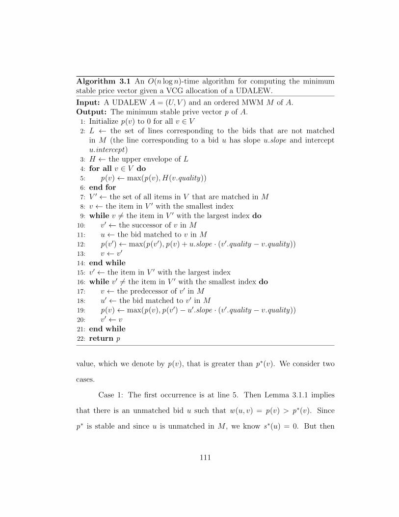
Algorithm 3.1 An O(n log n)-time algorithm for computing the minimumstable price vector given a VCG allocation of a UDALEW.

Input: A UDALEW A = (U, V ) and an ordered MWM M of A.Output: The minimum stable prive vector p of A.

1: Initialize p(v) to 0 for all v ∈ V2: L ← the set of lines corresponding to the bids that are not matched

in M (the line corresponding to a bid u has slope u.slope and interceptu.intercept)

3: H ← the upper envelope of L4: for all v ∈ V do5: p(v)← max(p(v), H(v.quality))6: end for7: V ′ ← the set of all items in V that are matched in M8: v ← the item in V ′ with the smallest index9: while v 6= the item in V ′ with the largest index do

10: v′ ← the successor of v in M11: u← the bid matched to v in M12: p(v′)← max(p(v′), p(v) + u.slope · (v′.quality − v.quality))13: v ← v′

14: end while15: v′ ← the item in V ′ with the largest index16: while v′ 6= the item in V ′ with the smallest index do17: v ← the predecessor of v′ in M18: u′ ← the bid matched to v′ in M19: p(v)← max(p(v), p(v′)− u′.slope · (v′.quality − v.quality))20: v′ ← v21: end while22: return p

value, which we denote by p(v), that is greater than p∗(v). We consider two

cases.

Case 1: The first occurrence is at line 5. Then Lemma 3.1.1 implies

that there is an unmatched bid u such that w(u, v) = p(v) > p∗(v). Since

p∗ is stable and since u is unmatched in M , we know s∗(u) = 0. But then

111

s∗(u) + p∗(v) < w(u, v), contradicting the stability of p∗.

Case 2: The first occurrence is at line 12 (resp., line 19) and we denote

the predecessor (resp., successor) of v by v′. Let u′ be the bid that is matched

to item v′ in M . Then, immediately after the price of v is set to p(v), we have

w(u′, v)−p(v) = w(u′, v′)−p(v′). Since this is the first time that the price for

an item exceeds its minimum stable price, we know that p(v′) ≤ p∗(v′), and

hence

w(u′, v)− p(v) ≥ w(u′, v′)− p∗(v′).

But, since p(v) > p∗(v), we have

w(u′, v)− p∗(v) > w(u′, v′)− p∗(v′),

contradicting the stability of p∗ since u′ is matched to v′ in M .

Hence the price of an item v is never increased beyond p∗(v).

Corollary 3.1.3. Let s∗ denote the utility vector corresponding to the mini-

mum stable prices. Then for any bid u, s(u) ≥ s∗(u) upon termination of the

algorithm.

Proof. Follows from the definition of s(u) and from Lemma 3.1.2.

Lemma 3.1.4. Let u be a bid in U that is unmatched in M , and let v be an

item in V . Then s(u) + p(v) ≥ w(u, v) upon termination of the algorithm.

Proof. Since u is not matched in M , we have s(u) = 0. Then the result follows

from Lemma 3.1.1 and from the fact that prices never decrease.

112

Lemma 3.1.5. Let v and v′ be two items in V such that both v and v′ are

matched and v′ is the successor of v in M . Let u denote the bid that is matched

to v and let u′ denote the bid that is matched to v′. Then s(u)+p(v′) ≥ w(u, v′)

and s(u′) + p(v) ≥ w(u′, v) upon termination of the algorithm.

Proof. First consider the claim s(u) + p(v′) ≥ w(u, v′). The first while loop

(lines 9 through 14) iterates through the items from lowest index to highest,

so it ensures that

p(v′) ≥ p(v) + u.slope · (v′.quality − v.quality)

= p(v) + w(u, v′)− w(u, v)

= w(u, v′)− s(u)

holds upon termination of the loop. The prices never decrease, so the claim

remains satisfied after any change to the price of item v′. We now show that

any increase to the price of item v does not violate the claim. Note that after

the first while loop (lines 9 through 14) is terminated, such an increase can

only happen once and it occurs in line 19. If it happens, the price of v is set

to:

p(v) = p(v′)− u′.slope · (v′.quality − v.quality)

= p(v′)− w(u′, v′) + w(u′, v). (3.1)

113

If this increase violates the claim, then we have

w(u, v)− p(v) + p(v′) < w(u, v′),

and substituting for p(v) from (3.1) gives

w(u, v) + w(u′, v′) < w(u, v′) + w(u′, v),

which contradicts that M is an MWM because switching the items assigned

to bids u and u′ results in a heavier matching.

Now consider the claim s(u′) + p(v) ≥ w(u′, v). The second while loop

(lines 16 through 21) iterates through the items from highest index to lowest,

so it ensures that

p(v) ≥ p(v′)− u′.slope · (v′.quality − v.quality)

= p(v′)− w(u′, v′) + w(u′, v)

= w(u′, v)− s(u′)

holds upon termination of the loop.

Lemma 3.1.6. Let u be a bid in U and let v be an item in V such that both

u and v are matched in M . Then s(u) + p(v) ≥ w(u, v) upon termination of

the algorithm.

Proof. If v is matched to u in M , then s(u) + p(v) = w(u, v) by definition.

Suppose that u is matched to some item v′ that is not equal to v. We give the

114

proof for the case where the index of v′ is smaller than that of v; the other

case is symmetric. Since the index of v′ is smaller than that of v, there exists a

unique sequence 〈v1, . . . , vk〉 of matched items in M such that v1 = v′, vk = v,

and vi+1 is the successor of vi in M for 1 ≤ i < k. Given such a sequence,

let P (i) denote the inequality s(u) + p(vi) ≥ w(u, vi). We show by induction

that P (k) holds. The base case P (2) is implied by Lemma 3.1.5 since v2 is

the successor of v1 = v′. Now assume that P (i) holds for some i such that

2 ≤ i < k. Let ui denote the bid to which item vi is matched. Since vi+1 is

the successor of vi, Lemma 3.1.5 implies that

s(ui) + p(vi+1) ≥ w(ui, vi+1).

Adding inequality P (i) to the preceding inequality we obtain

s(u) + p(vi) + s(ui) + p(vi+1) ≥ w(u, vi) + w(ui, vi+1),

and hence

s(u) + p(vi+1) ≥ w(u, vi) + w(ui, vi+1)− w(ui, vi)

since p(vi) + s(ui) = w(ui, vi).

115

By the definition of w(u, v), we have

w(u, vi) + w(ui, vi+1)− w(ui, vi) = w(u, vi) + ui.slope(vi+1.quality − vi.quality)

≥ w(u, vi) + u.slope(vi+1.quality − vi.quality)

= w(u, vi+1),

where the second line follows since vi+1.quality ≥ vi.quality and since the

assumption that M is an ordered MWM of A implies ui.slope ≥ u.slope.

Hence P (i+ 1) holds.

Lemma 3.1.7. Let u be a bid in U that is matched in M , and let v be an item

in V that is not matched in M . Then s(u) + p(v) ≥ w(u, v) upon termination

of the algorithm.

Proof. Let v′ be the item that is matched to u. Let p∗ denote the minimum

stable price vector and let s∗ denote the corresponding surplus vector. Then

s∗(u) + p∗(v) ≥ w(u, v). Since v is unmatched in M we have p∗(v) = 0. Thus,

Lemma 3.1.2 and the fact that the algorithm never sets a price to a negative

value together imply that p(v) = 0. Corollary 3.1.3 implies s(u) ≥ s∗(u).

Hence s(u) ≥ w(u, v), as required.

Theorem 3.1.8. The algorithm computes the minimum stable price vector

in O(n log n) time.

Proof. Since the algorithm maintains nonnegative prices, no item blocks M .

Corollary 3.1.3 implies that no bid blocks M . Lemmas 3.1.4, 3.1.6, and 3.1.7

116

together imply that no bid-item pair blocks M . By combining the preceding

observations we deduce that the final price vector is stable. Hence Lemma 3.1.2

implies that the final price vector is the minimum stable price vector.

The most expensive step in the algorithm is the computation of the

upper envelope of n lines. It is known that the lower convex hull of points

and the upper envelope of lines are dual to each other [13, Section 11.4]. Since

the lower convex hull can be computed in O(n log n) time [45, Theorem 3.7]

and the two while loops take linear time, the complexity of the algorithm is

O(n log n).

117

Chapter 4

UDALEWs with Evenly-Spaced

Qualities and Applications to

Scheduling

This chapter presents the three results mentioned in Section 1.1.2: Section 4.2

presents our O(n log n)-time algorithm for solving Problem 1.1; Section 4.3

describes how to use the algorithm of Section 4.2 to solve Problem 1.2 in

O(n log n) time; Section 4.4 shows that certain natural variations of Prob-

lem 1.1 are NP-hard. An abbreviated version of the results presented in this

chapter appears in a conference publication [15].

As mentioned in Section 1.1.2, Problem 1.1 is equivalent to the prob-

lem of computing a VCG allocation of a UDALEW where the item qualities

form an arithmetic sequence, and Problem 1.2 is equivalent to the problem of

118

computing a VCG allocation of a UDALEW where the item qualities form a

nondecreasing sequence that is the concatenation of two arithmetic sequences.

Since our interest in these special cases is motivated by the applications to

the scheduling domain, throughout this chapter, however, we deviate from the

terminology of Chapter 2 and we adopt a terminology that is common in such

applications.

We begin by revisiting Problems 1.1 and 1.2, and briefly reviewing re-

lated work. In both problems, we study scheduling unit jobs, i.e., jobs with

an execution requirement of one time unit, with individual weights (wi) and

profits (ei) on a single machine with a common deadline (d) where some jobs

may be rejected. If a job is scheduled by the deadline then its completion time

is denoted by Ci; otherwise it is considered rejected. Let S denote the set of

scheduled jobs and S denote the set of rejected jobs. In Problem 1.1, the goal

is to minimize the sum of the weighted completion times of the scheduled jobs

plus the total profits of the rejected jobs. Hence job profits can be equivalently

interpreted as rejection penalties. We represent this problem using Graham’s

notation [32] as:

1 | pi = 1, di = d |∑S

wiCi +∑S

ei . (1.1 revisited)

In Problem 1.2, we incorporate weighted tardiness penalties with respect to a

common due date, i.e., every job also has a common due date d, and completing

a job after the due date incurs an additional tardiness penalty that depends

on its weight and a positive constant c, where the tardiness of a job is defined

119

as Ti = max0, Ci − d. We represent this problem using Graham’s notation

as:

1 | pi = 1, di = d, di = d |∑S

wiCi + c∑S

wiTi +∑S

ei . (1.2 revisited)

In both problems, we assume that the number of jobs is at least d.

If not, letting U+ (resp., U−) denoting the set of the jobs with nonnegative

(resp., negative) weights, it is easy to observe that there exists a solution in

which each job in U+ (resp., U−) that is not rejected is scheduled in one of

the first |U+| (resp., last |U−|) slots. Using this observation, we can solve the

given instance by solving two smaller instances for which our assumption is

satisfied.

4.1 Related Work

More general cases of Problem 1.1, almost all dealing with variable processing

times, have been studied extensively. One of the earliest works that considers

job specific profits and lateness penalties [59] reduces to our problem in the

special case of setting all processing times to 1 and all due dates to 0. Two

recent surveys review the research on various scheduling problems in which it is

typically necessary to reject some of the jobs in order to achieve optimality [53,

58]. Epstein et al. [24] focus on unit jobs but consider only the online version

of the problem.

120

Engels et al. [23] give a pseudo-polynomial-time dynamic programming

algorithm for the same objective except that variable processing times are

allowed and no deadline restriction is imposed. Engels et al. first show that

the decision version of the problem is NP-complete and then give an FPTAS.

They also remark that a running time of O(n2) can be achieved for the special

case of unit processing times; our work improves this bound to O(n log n).

4.2 A Fast Algorithm for Problem 1.1

We encode an instance of Problem 1.1 as a weighted matching problem on a

graph drawn from a certain family. Below we define this family, which we call

G, and we discuss how to express an instance of Problem 1.1 in terms of a

graph in G.

We define G as the family of all complete edge-weighted bipartite graphs

G = (U, V, w) such that the following conditions hold: |U | ≥ |V |; each left

vertex u in U has two associated integers u.intercept and u.slope; the left

vertices are indexed from 1 in non-decreasing order of slopes, breaking ties

arbitrarily; right vertices are indexed from 1; the weight w(u, v) of the edge

between a left vertex u and a right vertex v is equal to u.intercept +u.slope · j

where j denotes the index of v. Note that a graph G = (U, V, w) in G admits an

O(|U |)-space representation. It is easy to see that the family G is equivalent

to the family of (graphs corresponding to the) all UDALEWs (modulo the

order of vertices, and the bid and item id ’s) such that the number of bids is at

least the number of items and the qualities of the items form the arithmetic

121

sequence 1 through the number of items.

Let I be an instance of Problem 1.1. The instance I consists of a set of

n jobs to schedule, each with a profit and a weight, and a common deadline d

where we assume that n ≥ d as discussed in the beginning of this chapter. We

encode the instance I as a graph G = (U, V, w) in G such that the following

conditions hold: |U | = n; |V | = d; each left vertex represents a distinct job in

I; each right vertex represents a time slot in which a job in I can be scheduled;

for each job in I and the vertex u that represents that job, u.intercept is equal

to the profit of the job and u.slope is equal to the negated weight of the job.

It is easy to see by inspecting the objective of Problem 1.1 that minimizing

the weighted sum of completion times is equivalent to maximizing the same

expression with negated weights, and minimizing the sum of the profits of

the rejected jobs is equivalent to maximizing the sum of the profits of the

scheduled jobs. Hence, instance I of Problem 1.1 is equivalent to the problem

of finding a maximum weight matching (MWM) of a graph G = (U, V, w) in G

that encodes I. Given this correspondence between the two problems, we refer

to the left vertices (resp., right vertices) of a graph in G as jobs (resp., slots).

The problem of computing an MWM of a graph G = (U, V, w) in G can be

reduced to the maximum weight maximum cardinality matching (MWMCM)

problem by adding |V | dummy jobs, each with intercept and slope zero, to

obtain a graph that also belongs to G.

As a result of the equivalence of the two problems mentioned above and

the reduction from the MWM to the MWMCM problem, we can obtain an

122

O(n log n)-time algorithm for Problem 1.1 by providing an O(|U | log |U |)-time

algorithm to compute an MWMCM of a graph G = (U, V, w) in G. Before

discussing this algorithm further, we introduce some useful definitions.

Let G = (U, V, w) be a graph in G. We say that a subset U ′ of U is

optimal for G if there exists an MWMCM M of G such that the set of jobs

that are matched in M is equal to U ′. Lemma 4.2.1 below shows that it is

straightforward to efficiently construct an MWMCM of G given an optimal

set of jobs for G. Let U ′ be a subset of U with size |V | and let i1 < · · · < i|V |

denote the indices of the jobs in U ′. Then we define matching(U ′) as the set

of |V | job-slot pairs obtained by pairing the job with index ik to the slot with

index k for 1 ≤ k ≤ |V |. The following lemma is analogous to Lemma 2.3.1

and it is a straightforward application of the rearrangement inequality [34,

Section 10.2, Theorem 368] to our setting.

Lemma 4.2.1. Let G = (U, V, w) be a graph in G. Let U ′ be a subset of

U with size |V |. Let W denote the maximum weight of any MCM of G that

matches U ′. Then matching(U ′) is of weight W .

Having established Lemma 4.2.1, it remains to show how to efficiently

identify an optimal set of jobs for a given graph G = (U, V, w) in G. The main

technical result of this section is an O(|U | log |U |)-time dynamic programming

algorithm for accomplishing this task. The following definitions are useful for

describing our dynamic programming framework.

Let G = (U, V, w) be a graph in G. For any integer i such that 0 ≤ i ≤

|U |, we define Ui as the set of jobs with indices 1 through i. Similarly, for any

123

integer j such that 0 ≤ j ≤ |V |, we define Vj as the set of slots with indices 1

through j. For any integers i and j such that 0 ≤ j ≤ i ≤ |U | and j ≤ |V |,

we define Gi,j as the subgraph of G induced by the vertices Ui ∪ Vj, and we

define W (i, j) as the weight of an MWMCM of Gi,j. Note that any subgraph

Gi,j of G also belongs to G.

Let us define G∗ as the family of all graphs in G having an equal number

of slots and jobs. Given a graph G = (U, V, w) in G∗, our dynamic program-

ming algorithm computes in O(|U | log |U |) total time an optimal set of jobs

for each G|U |,j for 1 ≤ j ≤ |U |. For any graph G′ = (U, V ′, w′) in G, we

can construct a graph G = (U, V, w) in G∗ satisfying G′|U |,j = G|U |,j for all

1 ≤ j ≤ |V ′| by defining V as the set of |U | slots indexed from 1 through |U |.

Thus, given any graph G′ = (U, V ′, w′) in G, our algorithm can be used to

identify an optimal set of jobs for each subgraph G′|U |,j for 1 ≤ j ≤ |V ′| in

O(|U | log |U |) total time.

Throughout the remainder of this section, we fix a graph instance

G = (U, V, w) in G∗. The presentation of the algorithm is organized as fol-

lows. Section 4.2.1 introduces the core concept, which we call the acceptance

order, that our algorithm is built on. Section 4.2.2 presents the key idea

(Lemma 4.2.7) underlying our algorithm for computing the acceptance order.

Finally, Section 4.2.3 describes an efficient augmented binary search tree im-

plementation of the algorithm.

124

4.2.1 Acceptance Orders

Lemma 4.2.1 reduces Problem 1.1 to the problem of identifying an optimal

subset of U for G. In addition to an optimal set of jobs for G, our algorithm

determines for each integer i and j such that 0 ≤ j ≤ i ≤ |U |, a subset

best(i, j) of Ui that is optimal for Gi,j (Lemma 4.2.5). There are quadratically

many such sets, so in order to run in quasilinear time, we compute a compact

representation of those sets by exploiting the following two properties. The

first property is that best(i, j − 1) is a subset of best(i, j) for 1 ≤ j ≤ i ≤ |U |.

Thus, for a fixed i, the sequence of sets best(i, 1), . . . , best(i, i) induces an

ordering σi of jobs Ui, which we later define as the acceptance order of Ui,

where the job at position j of σi is the one that is present in best(i, j) but not

in best(i, j − 1). The second property is that σi−1 is a subsequence of σi for

1 ≤ i ≤ |U |. This second property suggests an incremental computation of

σi’s which will be exploited to find the weights of MWMCMs for all prefixes

of jobs to solve Problem 1.2, as described in Section 4.3.

We now give the formal definitions of the acceptance order and the

optimal set best(i, j), and present two associated lemmas.

We say that a vertex is essential for an edge-weighted bipartite graph

G if it belongs to every MWMCM of G.

For any integer i such that 0 ≤ i ≤ |U | we define σi inductively as

follows: σ0 is the empty sequence; for i > 0 let u denote the job with index i,

then σi is obtained from σi−1 by inserting job u immediately after the prefix

of σi−1 of length p − 1 where p, which we call the position of u in σi, is the

125

minimum positive integer such that job u is essential for Gi,p. It is easy to see

that σi is a sequence of length i and that 1 ≤ p ≤ i since u is trivially essential

for Gi,i. Furthermore, σi−1 is a subsequence of σi for 1 ≤ i ≤ |U |, as claimed

above.

We say that σi is the acceptance order of the set of jobs Ui. Note that

σ|U | is the acceptance order of the set of all jobs.

The following lemma is used in the proof of Lemma 4.2.3.

Lemma 4.2.2. Let G = (U, V,E) be an edge-weighted bipartite graph, let V ′

be a subset of V , let G′ be the subgraph of G induced by the set of vertices

U ∪ V ′, and let u be a vertex in U that is essential for G′. Then u is essential

for G.

Proof. Assume that the claim is false, and let M be an MWMCM of G such

that u is not matched in M . Let M ′ be an MWMCM of G′. Since u is essential

for G′, vertex u is matched in M ′. Let G′′ denote the graph (U, V,M ⊕M ′).

Since u is matched in M ′ and not in M , we deduce that u has degree one in

G′′. Since no vertex in G′′ has degree more than two, we conclude that the

connected component of G′′ that includes u is a path, call it P , and that u is

an endpoint of P . The edges of P alternate between M and M ′; let X denote

P ∩M and let X ′ denote P ∩M ′.

Case 1: P is of odd length. Since u is an endpoint of P and is u is

matched in M ′, we deduce that |X ′| = |X| + 1. It follows that (M \X) ∪X ′

is a matching of G with cardinality one higher than that of M , contradicting

our assumption that M is an MWMCM of G.

126

Case 2: P is of even length. Thus |X| = |X ′| and every vertex in V

that belongs to P is matched in both M and M ′, and hence belongs to V ′. It

follows that (M ′ \X ′) ∪X is an MCM of G′; in what follows, we refer to this

MCM of G′ as M ′′. Let W denote the total weight of the edges in X and let

W ′ denote the total weight of the edges in X ′.

Case 2.1: W < W ′. Thus (M \X) ∪X ′ is an MCM of G with weight

higher than that of M , contradicting our assumption that M is an MWMCM

of G.

Case 2.2: W > W ′. Thus M ′′ is an MCM of G′ with weight higher than

that of M ′, contradicting our assumption that M ′ is an MWMCM of G′.

Case 2.3: W = W ′. Thus M ′′ is an MWMCM of G that does not match

u, contradicting our assumption that u is essential for G′.

Lemma 4.2.3. Let i and j be any integers such that 1 ≤ j ≤ i ≤ |U | and let

u denote the job with index i. Then job u is essential for Gi,j if and only if

the position of u in σi is at most j.

Proof. Immediate from Lemma 4.2.2.

For any integers i and j such that 0 ≤ j ≤ i ≤ |U |, we define best(i, j)

as the set of the first j jobs in σi. Thus, best(i, j − 1) is a subset of best(i, j)

for 1 ≤ j ≤ i ≤ |U |, as claimed above.

The following lemma is used in the proof of Lemma 4.2.5.

127

Lemma 4.2.4. For any integers i and j such that 1 ≤ j ≤ i ≤ |U |, we have

best(i, j) =

best(i− 1, j − 1) + u if job u is essential for Gi,j

best(i− 1, j) otherwise,

where u denotes the job with index i.

Proof. Immediate from the definition of best(i, j) and from Lemma 4.2.3.

Lemma 4.2.5. Let i and j be any integers such that 0 ≤ j ≤ i ≤ |U |. Then

matching(best(i, j)) is an MWMCM of Gi,j.

Proof. For any integer i such that 0 ≤ i ≤ |U |, let P (i) denote the predicate

“for any integer j such that 0 ≤ j ≤ i, matching(best(i, j)) is an MWMCM of

Gi,j”. We prove by induction on i that P (i) holds for all i such that 0 ≤ i ≤ |U |.

It is easy to see that P (0) holds. Let i be an integer such that 0 < i ≤ |U |,

and let u denote the job with index i. We now complete the proof by arguing

that P (i − 1) implies P (i). It is easy to see that matching(best(i, 0)) is an

MWMCM of Gi,0. Thus in the remainder of the argument we may assume

that j is an integer such that 1 ≤ j ≤ i. We consider two cases.

Case 1: Job u is essential for Gi,j. Let v denote the slot with index

j. By Lemma 4.2.1, and since the index of job u is greater than that of

any job in Gi−1,j−1, we can obtain an MWMCM of Gi,j by adding the edge

(u, v) to an arbitrary MWMCM of Gi−1,j−1. By the induction hypothesis,

matching(best(i − 1, j − 1)) is an MWMCM of Gi−1,j−1. Thus the matching

obtained by adding edge (u, v) to matching(best(i−1, j−1)) is an MWMCM of

128

Gi,j. Since Lemma 4.2.4 implies that best(i, j) is equal to best(i−1, j−1) +u,

and since the index of job u is greater than that of any job in best(i − 1, j −

1), the latter matching is equal to matching(best(i, j)). We conclude that

matching(best(i, j)) is an MWMCM of Gi,j, as required.

Case 2: Job u is not essential for Gi,j. Thus any MWMCM of Gi−1,j

is an MWMCM of Gi,j. By the induction hypothesis, we conclude that

matching(best(i − 1, j)) is an MWMCM of Gi,j. Since Lemma 4.2.4 implies

that best(i, j) is equal to best(i − 1, j), we conclude that matching(best(i, j))

is an MWMCM of Gi,j, as required.

Lemmas 4.2.1 and 4.2.5 imply that once we compute the acceptance

order σ|U |, we can sort its first d jobs by their indices to obtain a matching to

solve Problem 1.1.

4.2.2 Computing the Acceptance Order

As we have established the importance of the acceptance order σ|U |, we now

describe how to compute it efficiently. We start with σ1 and introduce the tasks

one by one in index order to compute the sequences σ2, . . . , σ|U | incrementally.

Once we know σi−1, we just need to find out where to insert the job with index

i in order to compute σi. We first introduce some definitions and a lemma,

and then we describe the key idea (Lemma 4.2.7) for finding the position of a

job in the corresponding acceptance order.

For any integers i and j such that 1 ≤ j ≤ i ≤ |U |, let σi[j] denote the

job with position j in σi, where σi[1] is the first job in σi.

129

For any job u that belongs to U , we define better(u) as the set of jobs

that precede u in σi where i denotes the index of u. Thus |better(u)| = p− 1

where p is the position of u in σi. The set better(u) is the set of jobs that

precede u both in index order and in acceptance order.

Lemma 4.2.6. Let i and j be integers such that 1 ≤ j ≤ i ≤ |U |, and let i′

denote the index of job σi[j]. Then the set of jobs in best(i, j− 1) with indices

less than i′ is equal to better(σi[j]).

Proof. Every job in best(i, j) has index at most i. Since σi[j] belongs to

best(i, j), we conclude that i′ ≤ i. Let p denote the position of σi[j] in σi′ .

By definition, job σi[j] occurs in position j of σi. By the definition of σi′ , job

σi[j] occurs in position p of σi′ . Since σi′ is a subsequence of σi, we conclude

that best(i, j− 1) consists of better(σi[j]) plus j− p additional jobs, each with

index greater than i′. Since each job in better(σi[j]) has index less than i′, the

claim follows.

For any subset U ′ of U , we define sum(U ′) as∑

u∈U ′ u.slope.

Now we are ready to discuss the idea behind the efficient computation

of the acceptance orders incrementally. Assume that we already know the

acceptance order σi−1 of the set of the first i− 1 jobs for some integer i such

that 1 < i ≤ |U |. Let u denote the job with index i. If we can determine in

constant time, for any job in the set Ui−1, whether u precedes that job in σi,

then we can perform a binary search in order to find in logarithmic time the

position of u in σi. Suppose that we would like to know whether u precedes

σi−1[j] in σi for some integer j such that 1 ≤ j < i. In other words we would

130

like to determine whether the position of u in σi is at most j. In what follows,

let u′ denote the job σi−1[j] and let v denote the slot with index j. Then by

Lemma 4.2.3, job u precedes u′ in σi if and only if u is essential for Gi,j.

In order to determine whether job u is essential for Gi,j, we need to

compare the weight of a heaviest possible matching for Gi,j that does not

include u to the weight of a heaviest possible matching for Gi,j that includes

u. The former weight is W (i− 1, j). Since job u has the highest index among

the jobs with indices 1 through i, by Lemma 4.2.1, the latter weight is equal

to w(u, v) + W (i− 1, j − 1).

Let X denote best(i−1, j−1). Since best(i−1, j−1)+u′ = best(i−1, j),

Lemma 4.2.5 implies that the weight of matching(X+u′) is equal to W (i−1, j).

By Lemma 4.2.5, the weight of matching(X) is W (i − 1, j − 1). Since job u

has the highest index among the jobs in X+u, the weight of matching(X+u)

is w(u, v) + W (i− 1, j − 1).

Combining the results of the preceding paragraphs, we conclude that

job u is essential for Gi,j if and only if the weight of matching(X+u) is greater

than the weight of matching(X + u′).

Figure 4.1 shows an example where i = 10 and j = 7. Thus we are

trying to determine whether the job with index 10 precedes σ9[7] in σ10. In

this example, u denotes the job with index 10 and u′ denotes σ9[7], which is

the job with index 5, as shown in Figure 4.1a. The set X is the first 6 jobs

in σ9. The jobs appearing past u′ in σ9, jobs with indices 7 and 2, do not

participate in the matchings that we are interested in so they are crossed out.

131

27513 46 89σ9

Xu′

better(u′)

(a) Acceptance order σ9

1 3 4 5 6 8 9

1 3 4 6 8 9 10

1 2 3 4 5 6 7Slotv′ v

matching(X + u′)

matching(X + u)

(b) The two matchings to compare

Figure 4.1: An example in which we try to determine whether the job withindex 10 precedes σ9[7] in σ10. Each box represents the job whose index isshown inside.

Figure 4.1b shows the two matchings matching(X + u′) and matching(X + u)

of which we would like to compare the weights. As seen in Figure 4.1b, each

job in X with index less than that of job u′, shaded light gray in the figure,

is matched to the same slot in both matching(X + u) and matching(X + u′).

By Lemma 4.2.6, those jobs are the ones in the set better(u′), which are the

jobs with indices 1, 3 and 4 in the example. Hence job u′ occurs in position

|better(u′)| + 1 when we sort the set of jobs X + u′ by index and thus it is

matched to the slot with index |better(u′)|+1 in matching(X+u′). Moreover,

each job in X with index greater than that of job u′ is matched to a slot with

index one lower in matching(X +u) than in matching(X +u′), as depicted by

the arrows in Figure 4.1b for the jobs with indices 6, 8, and 9.

Hence the weight of matching(X+u) minus the weight of matching(X+

u′) is equal to w(u, v) − w(u′, v′) plus the sum of the slopes of all jobs in

best(i − 1, j − 1) with indices greater than that of u′, where v′ denotes the

slot with index |better(u′)| + 1. By Lemma 4.2.6, the latter sum is equal to

sum(best(i − 1, j − 1)) − sum(better(u′)). These observations establish the

132

proof of the following lemma which we utilize in computing the acceptance

orders incrementally.

Lemma 4.2.7. Let i and j be integers such that 1 ≤ j < i ≤ |U |. Let

u denote the job with index i and let u′ denote the job σi−1[j]. Then the

following are equivalent: (1) The position of u in σi is at most j; (2) Job

u is essential for Gi,j; (3) The weight of matching(best(i − 1, j − 1) + u) is

greater than the weight of matching(best(i − 1, j − 1) + u′); (4) w(u, v) >

w(u′, v′) + sum(best(i − 1, j − 1)) − sum(better(u′)) where v denotes the slot

with index j and v′ denotes the slot with index |better(u′)|+ 1.

4.2.3 Binary Search Tree Implementation

We employ a self-balancing binary search tree (BST) that stores the jobs in

a certain order: an inorder traversal of the BST yields the acceptance order.

We obtain an efficient algorithm for incrementally computing the acceptance

orders by augmenting this BST so that we can apply Lemma 4.2.7 in constant

time. The algorithm runs |U | iterations where the job with index i is inserted

into the BST at iteration i to obtain σi from σi−1 by performing a binary

search. We first give some definitions that are useful in the description of the

algorithm and then we state in Lemma 4.2.8 how to perform the comparisons

for the binary search.

For a binary tree T and an integer i such that 1 ≤ i ≤ |U |, we define

the predicate ordered(T, i) to hold if T contains i nodes that represent the jobs

Ui, and the sequence of the associated jobs resulting from an inorder traversal

133

of T is σi. The job represented by a node x is denoted by x.job.

Let T be a binary tree satisfying ordered(T, i) for some i. For any node

x in T , precede(x, T ) is defined as the set of jobs associated with the nodes

that precede x in an inorder traversal of T .

Lemma 4.2.8. Let i be an integer such that 1 < i ≤ |U | and let u denote the

job with index i. Let T be a binary tree satisfying ordered(T, i−1) and let x be

a node in T . Assume that |precede(x, T )|, sum(precede(x, T )), |better(x.job)|,

and sum(better(x.job)) are given. Then we can determine in constant time

whether u precedes x.job in σi.

Proof. Let j denote |precede(x, T )| + 1. Then ordered(T, i − 1) implies that

x.job is σi−1[j] and sum(precede(x, T )) is equal to sum(best(i−1, j−1)). Now

let u′ denote σi−1[j]. Then we can test Inequality 4 of Lemma 4.2.7 in constant

time to determine whether the position of u in σi is at most j, thus whether

u precedes u′ in σi.

Lemma 4.2.8 implies that once we know certain quantities about a node

x in the BST then we can tell in constant time whether the new job precedes

x.job in the acceptance order. The necessary information to compute the first

two of those quantities can be maintained by standard BST augmentation

techniques as described in [11, Chapter 14]. The other two quantities turn out

to be equal to the first two at the time the node is inserted into the BST and

they can be stored along with the node. In order to present the details of our

algorithm and how we augment the BST, we introduce the following useful

definitions.

134

We define T as the set of all binary trees T satisfying the following two

conditions: (1) the predicate ordered(T, i) holds for some i; (2) each node x

in T has integer fields x.size, x.sum, x.sizeLeft , and x.sumLeft (in addition to

the field x.job implied by condition (1)).

For any tree T in T and any node x in T , we define subtree(x) as the

set of all jobs that are associated with the nodes in the subtree rooted at x.

For convenience we define subtree(nil) as the empty set.

For any tree T in T and any node x in T , we define the predicate

augmented(x) to hold if the field x.size is equal to |subtree(x)|, and the field

x.sum is equal to sum(subtree(x)). We refer to x.size and x.sum together as

the augmented fields of node x.

For any tree T in T and any node x in T , we define the predicate

historical(x) to hold if the field x.sizeLeft is equal to |better(x.job)|, and the

field x.sumLeft is equal to sum(better(x.job)). We refer to x.sizeLeft and

x.sumLeft together as the historical fields of node x.

For any tree T in T and any integer i, we define the predicate

represent(T, i) to hold if ordered(T, i) holds, and for every node x in T , both

augmented(x) and historical(x) hold.

Our algorithm grows an augmented BST by iteratively inserting each

of the |U | jobs, in index order. A concise implementation is given in Algo-

rithm 4.1. The outer while loop (lines 3–32) runs for |U | iterations. Each

iteration i inserts the job with index i, referenced by the variable u, into

the BST, whose root is pointed by the variable x at the beginning of the

135

iteration. The inner while loop (lines 8–18) performs the binary search by

starting from the root and descending to the insertion position of the new

leaf representing the job u. When the execution reaches line 14, the vari-

able sizeLeft ′ is equal to |precede(x, T )| and the variable sumLeft ′ is equal to

sum(precede(x, T )). The variable flag is set depending on the outcome of the

application of Lemma 4.2.8.

Lines 19–30 attach the new leaf y to the BST and set its historical fields.

The Fixup routine, which is called at line 31, fixes the augmented fields of the

nodes along the path from the new leaf to the root, rebalances the BST using

the standard techniques of the associated self-balancing BST implementation,

and returns the root of the BST. (For a red-black tree implementation, the

Fixup routine can be implemented as the RB-Insert-Fixup operation [11,

Chapter 13] with the addition of setting the new node’s color to red at the

beginning, following the guidelines in [11, Chapter 14] for the augmentation.)

Thus, at the end of each iteration of the outer while loop, the BST stores the

jobs inserted so far in their acceptance order.

Theorem 4.2.9. Algorithm 4.1 computes the acceptance order of U in

O(|U | log |U |) time.

Proof. Let Ti denote the BST obtained by the algorithm after i iterations,

1 ≤ i ≤ |U |. We establish below that represent(Ti, i) holds for 1 ≤ i ≤ |U |.

Given this claim, it is easy to verify that the historical fields of a node x

remain constant after the initial creation of x. Thus the historical fields could

just as easily be maintained in an array outside of the tree. In contrast, the

136

Algorithm 4.1 An efficient algorithm for incrementally computing the ac-ceptance order by growing an augmented BST.

Input: A set U of jobs (sorted in non-decreasing order of slopes).1: x← nil2: i← 03: while i < |U | do4: i← i+ 15: u← the job from the set U with index i6: sizeLeft , sumLeft ← 07: x′ ← x8: while x′ 6= nil do9: x← x′

10: sizeLeft ′ ← if x.left = nil then sizeLeft else sizeLeft + x.left .size11: sumLeft ′ ← if x.left = nil then sumLeft else sumLeft + x.left .sum12: v ← the slot with index sizeLeft ′ + 113: v′ ← the slot with index x.sizeLeft + 114: flag ← w(u, v) ≤ w(x.job, v′) + sumLeft ′ − x.sumLeft15: x′ ← if flag then x.right else x.left16: sizeLeft ← if flag then sizeLeft ′ + 1 else sizeLeft17: sumLeft ← if flag then sumLeft ′ + x.job.slope else sumLeft18: end while19: y ← a new tree node20: y.job ← u21: y.sizeLeft ← sizeLeft22: y.sumLeft ← sumLeft23: y.parent ← x24: if x 6= nil then25: if flag then26: x.right ← y27: else28: x.left ← y29: end if30: end if31: x← Fixup(y)32: end while

137

augmented fields form an integral part of the BST data structure, and may be

updated as the structure of the tree changes.

We use a red-black tree to obtain the desired time bound. Cormen

et al. [11, Chapters 13 and 14] present an implementation for red-black trees

that rebalances the tree in logarithmic time while maintaining the augmented

fields.

First we state an observation that will be utilized in the constant time

comparison of the nodes and in the computation of the historical fields. Let

T be a tree in T such that each node x in T satisfies augmented(x). Then

observe that we can compute |precede(r, T )| and sum(precede(r, T )) in constant

time where r denotes the root of T . Moreover, for each non-root node x in

T , |precede(x, T )| and sum(precede(x, T )) can be computed in constant time

given |precede(y, T )| and sum(precede(y, T )) where y denotes the parent of x.

The first iteration of the algorithm creates a BST T1 with a single node

x representing the job with index 1. The two historical fields of x are each

initialized to zero, and the augmented fields are initialized as follows: x.size is

set to 1; x.sum is set to the slope of the job with index 1. It is easy to verify

that the predicate represent(T1, 1) holds.

We now describe a non-first iteration i, 1 < i ≤ |U |, where we assume

inductively that represent(Ti−1, i−1) holds. Let u denote the job with index i.

In order to obtain Ti from Ti−1, we first insert a new leaf representing the job

u into Ti−1 without changing the structure of Ti−1 other than linking the new

leaf such that the resulting BST, call it T ′i−1, satisfies ordered(T ′i−1, i). Note

138

that there is a unique such BST T ′i−1 since there is a unique position in the

tree such that the new node representing u can be inserted without changing

the edges between the existing nodes. This insertion position can be found by

first comparing the job u with the job represented by the root of Ti−1 (apply-

ing Lemma 4.2.8) and descending either left or right depending on whether u

precedes the root in σi, thus following a path that terminates at the insertion

position by comparing u with the jobs represented by the nodes on that path

as in a standard BST insertion operation. By the observation in the previous

paragraph, it is easy to see that |precede(x, Ti−1)| and sum(precede(x, Ti−1))

can be computed in constant time for each node x on the path that the binary

search follows. Thus, together with the historical fields, we have the informa-

tion to apply Lemma 4.2.8 in constant time for each comparison. Let y denote

the new leaf that represents the job u. Again by the observation in the previ-

ous paragraph, since the last node that we compare u with is the parent of y,

|precede(y, T ′i−1)| and sum(precede(y, T ′i−1)) can also be computed in constant

time. Since ordered(T ′i−1, i) implies better(y.job) is equal to precede(y, T ′i−1),

the historical fields of y can be computed in constant time.

The process described above, which attaches the new leaf y representing

the job with index i to Ti−1 to obtain T ′i−1, takes time proportional to the

depth of y in T ′i−1. Once y is added, we can update the augmented fields of

the nodes on the path from y to the root within the same time bound so that

augmented(x) holds for each node x on that path. Note that the augmented

fields of the other nodes are not affected by the insertion, thus represent(T ′i−1, i)

139

holds.

The final step at iteration i is to rebalance T ′i−1 with the RB-Insert-Fixup

operation [11, Chapters 13 and 14] in logarithmic time, while maintaining the

augmented fields, in order to obtain O(|U | log |U |) overall running time. Let

Ti denote the result of the rebalancing operation on T ′i−1. Since the aug-

mented fields are maintained by the rebalancing operation, the BST Ti sat-

isfies represent(Ti, i) and the algorithm proceeds to the next iteration. Note

that it is easy to argue the same performance for certain other balanced BST

structures, e.g., O(|U | log |U |) amortized time for splay trees [57] where each

insertion, together with the associated splay operation at the end of each it-

eration, takes amortized logarithmic time.

As mentioned earlier, once σ|U | is computed, we can extract an MWMCM

of G|U |,j for any j such that 1 ≤ j ≤ |U |. If we are only interested in solutions

for j up to some given m, then the algorithm can be implemented in O(n logm)

time by keeping at most m nodes in the BST. We achieve this by deleting the

rightmost node when the number of nodes exceeds m. Note that if the jobs

are not already sorted by slopes then we still need to spend O(n log n) time.

If we would like to find out the weights of the MWMCMs of G|U |,j for

all j such that 1 ≤ j ≤ |U |, a naive approach would be to sort all prefixes of

σ|U | and to compute the weights. Section 4.2.4 explains how to compute all

those weights incrementally in linear time.

140

4.2.4 Incrementally Computing the Weights for All Pre-

fixes of Slots

Let n denote |U |. Once we have computed σn, we know a set of jobs that

forms an MWMCM of each Gn,j for 1 ≤ j ≤ n, but we are not readily given

the weight W (n, j) of such a matching. In this section, we describe how

to compute the weights W (n, 1), . . . ,W (n, n) incrementally in linear time

by scanning through σn. It is straightforward to compute W (n, 1). When

we inspect the job at position j in σn (which is σn[j]), we can compute

W (n, j) in constant time from W (n, j − 1) because Lemma 4.2.5 implies that

we can construct an MWMCM for Gn,j, namely matching(best(n, j)), from

matching(best(n, j − 1)), which is an MWMCM for Gn,j−1, by introducing

σn[j]. Let u′ denote σn[j] and let i′ denote the index of σn[j]. The change

in weight caused by introducing job u′ to matching(best(n, j − 1)) in order

to construct matching(best(n, j)) has two components: (1) w(u′, v′) where v′

denotes the slot with index |better(u′)|+1, since Lemma 4.2.6 implies that job

u′ is matched to the slot with index |better(u′)| + 1 in matching(best(n, j));

(2) the sum of the slopes of all jobs in best(n, j) with indices greater than

that of u′, since each such job is matched to a slot with index one higher in

matching(best(n, j)) than in matching(best(n, j − 1)) and every other job is

matched to the same slot in both matchings. By Lemma 4.2.6, the latter sum

is equal to sum(best(n, j − 1))− sum(better(i′)). Since we scan the jobs in σn

starting from position 1, we can maintain the sum of the slopes of the jobs

scanned so far, thus we know sum(best(n, j − 1)) when we reach job u′. We

141

already store |better(u′)| and sum(better(i′)) at the node representing u′, thus

the change in weight caused by introducing the job u′ can be computed in

constant time.

4.3 Introducing Tardiness Penalties

Consider the following extension to the complete bipartite graphsG = (U, V, w)

introduced in Section 4.2. For each slot (right vertex) v in V , we introduce

an integer parameter v.quality . We assume that the slots are indexed from

1 in non-decreasing order of qualities, breaking ties arbitrarily. We also as-

sume that the qualities of the slots form a non-decreasing sequence that is the

concatenation of two arithmetic sequences. We allow an arbitrary number of

slots that is less than the number of jobs. We modify the edge weights so that

w(u, v) between job u and slot v becomes u.intercept + u.slope · v.quality . We

are able to solve the MWM problem in such a graph instance in O(n log n)

time, which enables us to solve Problem 1.2 in O(n log n) time. The key idea

is to utilize the incremental computation of the acceptance orders so that we

can find the weights of the MWMCMs between the slots whose qualities form

the first arithmetic sequence (the slots before the common due date) and every

possible prefix of jobs. Then we do the same between the slots whose qualities

form the second arithmetic sequence (the slots after the common due date) and

every possible suffix of jobs. Then in linear time we find an optimal matching

by determining which jobs to assign to the first group of slots and which jobs

to the second group.

142

We start by introducing two families of graphs, H and H∗: H is equiv-

alent to UDALEWs (modulo the order of vertices, and the bid and item id ’s)

and it extends the family G by introducing qualities to the slots; H∗ is the

family of graphs mentioned in the previous paragraph and it consists of the

graphs on which we encode the instances of Problem 1.2 as weighted matching

problems. Then we discuss an algorithm that solves the MWMCM problem

on graphs drawn from the family H∗.

We defineH as the family of all complete edge-weighted bipartite graphs

G = (U, V, w) such that the following conditions hold: |U | ≥ |V |; each job u

in U has two associated integers u.intercept and u.slope; the jobs are indexed

from 1 in non-decreasing order of slopes, breaking ties arbitrarily; each slot v

in V has an associated integer v.quality ; the slots are indexed from 1 in non-

decreasing order of qualities, breaking ties arbitrarily; the weight w(u, v) of

the edge between a job u and a slot v is equal to u.intercept +u.slope ·v.quality .

Note that a graph G = (U, V, w) in H admits an O(|U |)-space representation.

Also note that an input graph G = (U, V, w) to the algorithm presented in

Section 4.2 can be interpreted as a graph belonging to the family H that has

|U | slots with qualities forming the arithmetic sequence 〈1, . . . , |U |〉. Observe

that the same algorithm can also be used to find an MWMCM for the case in

which the qualities form a different arithmetic sequence by scaling the slopes,

setting qualities to the arithmetic sequence 〈1, . . . , |U |〉, and modifying the

intercepts.

We now introduce the notion of a “splitting point”, a key technical

143

concept that underlies our algorithm. Let G = (U, V, w) be a graph in H.

We define Ui, Vj, and Gi,j in the same manner as we did for a graph in G in

Section 4.2. For any integer i such that 1 ≤ i < |U |, we define U−i as the set

U \Ui. Similarly for any integer j such that 1 ≤ j < |V |, we define V−j as the

set V \ Vj. For any integers i and j such that 1 ≤ j ≤ i < |U | and j < |V |, we

define G−i,−j as the subgraph of G induced by the vertices U−i ∪ V−j. Then

it is not hard to see that for any j in the range 1 ≤ j < |V |, there exists at

least one integer i, which we call a splitting point for j, such that the union

M1∪M2 is an MWMCM of G where M1 is any MWMCM of Gi,j and M2 is any

MWMCM of G−i,−j. Note that if i is a splitting point for j, then |Ui| ≥ |Vj|

and |U−i| ≥ |V−j|.

We encode an instance of Problem 1.2 as a weighted matching problem

on a graph drawn from a family H∗ that is contained in H. We define H∗ as

the family of all graphs G = (U, V, w) in H such that the qualities of the slots

in V , when visited in index order, form a non-decreasing sequence that is the

concatenation of two arithmetic sequences.

Let I be an instance of Problem 1.2. The instance I consists of a

set of n jobs to schedule, each with a profit and a weight; a common due

date d and a common deadline d where we assume that d < d ≤ n; and a

positive constant c. We encode the instance I as a graph G = (U, V, w) in

H∗ such that the following conditions hold: |U | = n; |V | = d; each u in U

represents a distinct job in I; each v in V represents a distinct time slot in

which a job in I can be scheduled; for each job in I and the vertex u that

144

represents that job, u.intercept is equal to the profit of the job and u.slope

is equal to the negated weight of the job; the qualities of the slots in V are

set to form the concatenation of the arithmetic sequences 〈1, 2, . . . , d〉 and

〈d + 1 + c, d + 2 + 2c, . . . , d + (d − d)c〉. It is easy to see by inspecting the

objective of Problem 1.2 that the instance I of Problem 1.2 is equivalent to the

problem of finding an MWM of a graph G = (U, V, w) in H∗ that encodes I.

Analogous to the case for G discussed in Section 4.2, the problem of finding an

MWM of a graph in H∗ can be reduced to the MWMCM problem by adding

dummy jobs.

We now describe our algorithm for computing an MWMCM of a graph

G = (U, V, w) in H∗. Let j denote the index such that the qualities of both

Vj and V−j are arithmetic sequences. If we can find the weights of MWMCMs

of each Gi,j for j ≤ i ≤ |U | and the weights of MWMCMs of each G−i,−j for

1 ≤ i ≤ |U | − |V |+ j in O(|U | log |U |) total time, then it takes linear time to

find a splitting point for j, and thus an MWMCM of G can be constructed in

O(|U | log |U |) total time.

Our algorithm consists of two extensions to the algorithm introduced

for Problem 1.1. Let G′ = (U, V ′, w) be a graph in H such that the qualities of

V ′ form an arithmetic sequence. In the remainder of this section, we use the

shorthand G′i (resp., G′−i) to denote the subgraph of G′ induced by the vertices

Ui ∪ V ′ (resp., U−i ∪ V ′) for any integer i such that 1 ≤ i ≤ |U |. The first

extension, which we discuss in the next paragraph, exploits the incremental

computation of the acceptance orders performed by the algorithm introduced

145

for Problem 1.1, in order to compute the weights of MWMCMs of each G′i for

|V ′| ≤ i ≤ |U | in O(|U | log |U |) total time. The second extension, which we

discuss in the final paragraph, finds the weights of MWMCMs of each G′−i for

1 ≤ i ≤ |U |−|V ′| in O(|U | log |U |) total time by a simple reduction so that the

first extension is utilized. Then, by setting G′ to the subgraph of G induced

by the vertices U ∪ Vj (resp., U ∪ V−j) as an input to the first (resp., second)

extension, these two extensions are used to find the weights of the MWMCMs

of each Gi,j for j ≤ i ≤ |U | and the weights of MWMCMs of each G−i,−j

for 1 ≤ i ≤ |U | − |V | + j in O(|U | log |U |) total time in order to compute an

MWMCM of a graph G = (U, V, w) in H∗.

First we show how to modify the algorithm introduced for Problem 1.1

so that we can compute the weights of MWMCMs of each subgraph G′i for

|V ′| ≤ i ≤ |U | given a graph G′ = (U, V ′, w) in H such that the qualities

of V ′ form an arithmetic sequence. As a preprocessing step, we scale the

slopes and modify the intercepts so that the instance G′ is transformed such

that the qualities form the arithmetic sequence 〈1, . . . , |V ′|〉, as mentioned in

the observation after the definition of H. In what follows, let T denote the

BST that the algorithm introduced for Problem 1.1 maintains. We modify the

algorithm so that we keep at most |V ′| nodes in T by discarding the rightmost

node when necessary, as mentioned in Section 4.2.3. Due to these deletions,

represent(T, i) no longer holds for i > |V ′|. However, it is easy to argue that,

for i > |V ′|, the BST T in the modified algorithm contains the first |V ′| jobs

in σi (i.e., best(i, |V ′|)), and that these jobs occur in the same order (with

146

respect to an inorder traversal) as in the BST in the unmodified algorithm.

For any integer i such that i ≥ |V ′|, let Mi denote matching(best(i, |V ′|)).

Then Lemma 4.2.5 implies that Mi is an MWMCM of G′i. We maintain an

additional BST τ that concurrently stores the same set of jobs that are present

in the main BST T , however in a different order. The keys of the nodes in

τ are the indices of the corresponding jobs, thus an inorder traversal of τ

yields an increasing order of indices. We implement τ as a balanced BST

and augment it so that we can query for the sum of the slopes of all jobs

that have indices greater than that of a given job. All the insert, delete,

and query operations can be implemented in logarithmic time using standard

augmentation techniques [11, Chapter 14]. We utilize those queries in order

to maintain the weight of Mi at each iteration i ≥ |V ′| in the following way.

First, the weight of M|V ′| can be computed at the end of iteration |V ′| via an

inorder traversal of τ . Now suppose that at the end of some iteration i for

i > |V ′|, the set of jobs in T is changed by an update consisting of insertion

of job u, which is the job with index i, to T (also to τ) and removal of some

job u′ from T (also from τ). Let τi−1 denote the state of the BST τ before this

update. Let j′ be the index of the slot that is matched to u′ in Mi−1. Note that

j′ is the rank of u′ in τi−1. Let U ′ denote the set of jobs in τi−1 with indices

greater than that of u′. Since u has the highest index among the jobs that

are matched in Mi, each job in U ′ is matched to a slot with index one lower

in Mi than in Mi−1, and every other job that is matched in Mi−1 except u′ is

matched to the same slot in Mi. Then, the weight of Mi minus the weight of

147

Mi−1 is equal to u.intercept +u.slope ·|V ′|−u′.intercept−u′.slope ·j′−sum(U ′).

Since such an update to τ and a query for sum(U ′) in τ can be performed in

O(log |V ′|) time, we can maintain the weight of each Mi for i ≥ |V ′| without

slowing down the algorithm asymptotically.

In order to compute the weights of MWMCMs of each subgraph G′−i for

1 ≤ i ≤ |U | − |V ′| given a graph G′ = (U, V ′, w) in H such that the qualities

of V ′ form an arithmetic sequence, we create another instance G′′ by negating

both the job slopes and slot qualities, and by reindexing both the jobs and the

slots in reverse orders. Then we run the algorithm described in the previous

paragraph on G′′. Note that the weight of the edge between the job with an

index i and the slot with an index j in G′′ is equal to the weight of the edge

between the job with index |U | − i + 1 and the slot with index |V ′| − j + 1

in G′. Thus the weight of an MWMCM of G′′i is equal to the weight of an

MWMCM of G′−|U |+i for |V ′| ≤ i < |U |.

4.4 NP-Hardness Results

It is natural to consider certain other problems within the setting of Prob-

lem 1.1, but with the goal of optimizing various other related criteria, possibly

by imposing some constraints. Shabtay et al. [52] split the scheduling objec-

tive into two criteria: the scheduling cost f , which depends on the completion

times of the jobs, and the rejection cost g, which is the sum of the penalties

paid for the rejected jobs. In addition to the problem of minimizing f + g,

Shabtay et al. also analyze the following two problems: minimization of f

148

subject to g ≤ R, where R is a given upper bound on the rejection cost; mini-

mization of g subject to f ≤ K, where K is a given upper bound on the value

of the scheduling criterion. In this section, we show that Problem 1.1 becomes

NP-hard if we split our criteria in the same manner and aim for optimizing

one while bounding the other.

Recall that the input to Problem 1.1 may be viewed as a graph G =

(U, V, w) in G where the weight w(u, v) of an edge between a job u in U and

a slot v in V with an index j is equal to u.intercept + u.slope · j. We split

the expression w(u, v) = u.intercept + u.slope · j denoting the weight of an

edge (u, v) into two summands: the first term u.intercept , which we call the

profit component ; the second term u.slope · j, which we call the scheduling

component. For a given MCM M of a graph G in G, we define f(G,M) as

the sum of the scheduling components of the weights of the edges in M , and

we define g(G,M) as the sum of the profit components of the weights of the

edges in M .

Given a graph G in G, let MG denote the set of all MCMs of G. Then

we define the following three problems, which are analogous to the problems

mentioned above from [52].

• P1: Find a matching M in MG maximizing f(G,M) + g(G,M).

• P2: Find a matchingM inMG maximizing f(G,M) subject to g(G,M) ≥

R.

• P3: Find a matchingM inMG maximizing g(G,M) subject to f(G,M) ≥

149

K.

The algorithm we introduced for Problem 1.1 solves P1 in O(n log n)

time, where n denotes the number of jobs in G. In this section, we show that

P2 and P3 are NP-hard. We define the decision version of both P2 and P3 as

follows: Given a graph G in G and two integers K and R, is there an MCM

M of G such that f(G,M) ≥ K and g(G,M) ≥ R? In what follows, we refer

to this decision problem as DP.

We show the NP-hardness of P2 and P3 by reducing the partition prob-

lem, which is known to be NP-complete, to DP. The partition problem is

defined as follows: Given a sequence ρ of m positive integers 〈ρ1, . . . , ρm〉 with

sum∑m

i=1 ρi = 2W , is there a subsequence of ρ with sum W? We assume

m ≥ 2 and ρi ≤ W for all 1 ≤ i ≤ m.

Throughout the remainder of the section, we fix an arbitrary instance

ρ of this partition problem. We now describe how to transfer ρ to an instance

(G,K,R) of DP. Our description introduces a variety of symbols, all of which

are fixed in value, throughout the remainder of this section.

Let m denote the size of ρ. Let W denote 12

∑mi=1 ρi. For any integer i

such that 1 ≤ i ≤ m, let Ai denote −2i−1W . Note that Ai =∑i−1

j=1Aj −W .

For any integer i such that 1 ≤ i ≤ m, let Bi denote 3iW .

Let G be a graph in G with a set U of 2m jobs ui, . . . , u2m, and a set

V of m slots vi, . . . , vm, and where the intercepts and slopes are determined

as follows. For any i such that 1 ≤ i ≤ m, we define the intercept of job u2i−1

as a2i−1 = Ai, the intercept of job u2i as a2i = Ai−ρi, the slope of job u2i−1 as

150

b2i−1 = Bi, and the slope of job u2i as b2i = Bi + ρii. Thus, for a given MCM

M of G,

f(G,M) =∑

(ui,vj)∈M

bi · j,

and

g(G,M) =∑

(ui,vj)∈M

ai.

Let K denote∑m

i=1 iBi + W , and let R denote∑m

i=1Ai −W = −2mW . It is

straightforward to verify that (G,K,R) is a DP instance, and the transforma-

tion from ρ to (G,K,R) can be performed in polynomial time.

Lemma 4.4.1. If ρ is a positive instance of the partition problem, then

(G,K,R) is a positive instance of DP.

Proof. Assume that ρ is a positive instance of the partition problem. Let

S be a subsequence of ρ with sum W . We construct an MCM M of G as

follows: For any i such that 1 ≤ i ≤ m, if ρi is in S then match u2i with vi;

otherwise, match u2i−1 with vi. It is easy to verify that f(G,M) = K and

g(G,M) = R.

Lemma 4.4.2. Let U ′ be a size-m subset of U . Then among all the MCMs ofG

matching the jobs U ′, there is a unique matching M that maximizes f(G,M),

and this unique M matches the jobs to the slots v1, . . . , vm in increasing order

of indices.

Proof. Observe that bi > bi−1 for any i such that 1 < i ≤ 2m. Hence the slopes

of the jobs in U ′ are distinct. Then the result follows from the rearrangement

151

inequality [34, Section 10.2, Theorem 368].

The following technical lemma is used in the proof of Lemma 4.4.4.

Lemma 4.4.3.∑i

j=1 jbi+j−2 ≤ iBi.

Proof. For any j such that 1 ≤ j ≤ m − 1, we have (j + 1)b2j + jb2j−1 ≤

2(j + 1)Bj since

(j + 1)b2j + jb2j−1 = (j + 1)

(Bj +

ρjj

)+ jBj

≤ (j + 1)Bj + 2ρj + (j + 1)Bj −Bj

≤ 2(j + 1)Bj + 2W − 3W

≤ 2(j + 1)Bj.

Thus

i∑j=1

jbi+j−2 ≤i−1∑j=1

(j + 1)b2j + jb2j−1

≤ 2i−1∑j=1

(j + 1)Bj

≤ 2iBi−1∑j≥0

3−j

= 3iBi−1

= iBi.

152

Lemma 4.4.4. LetM be an MCM ofG such that f(G,M) ≥ K and g(G,M) ≥

R. If (G,K,R) is a positive instance of DP, then for each i such that 1 ≤ i ≤ m,

exactly one of u2i−1 and u2i is matched in M , and it is matched to vi.

Proof. Assume that (G,K,R) is a positive instance of DP. Let P1(i) denote

the predicate “at least one of the jobs u2i−1 and u2i is matched in M”, and let

P2(i) denote the predicate “at most one of the jobs u2i−1 and u2i is matched

in M”. Then we claim the following.

Claim 1: If∧mj=i+1 (P1(j) ∧ P2(j)) holds for some integer i such that

1 ≤ i ≤ m, then P1(i) holds. It is easy to prove the claim for i = 1. Let

i be an integer such that 1 < i ≤ m and assume that the claim does not

hold. Then,∧mj=i+1 (P1(j) ∧ P2(j)) holds and neither u2i−1 nor u2i is matched

in M . We derive an upper on f(G,M) as follows. Let U ′ denote the set of

jobs that are matched in M . We know that U ′ consists of exactly one job

from each pair (u2j−1, u2j) for i < j ≤ m, and i other jobs having indices less

than 2i− 1. Lemma 4.4.2 implies that the unique MCM M ′ that matches U ′

and that maximizes f(G,M ′) has the following structure: for all i < j ≤ m,

the job from the pair (u2j−1, u2j) that is present in U ′ is matched to the slot

vj; the remaining i jobs in U ′ are assigned to the slots v1, . . . , vi in increasing

order of indices. Let M∗ denote this unique MCM, thus f(G,M) ≤ f(G,M∗).

We construct another matching M ′′ by assigning u2j to vj for i < j ≤ m,

and by assigning ui−1, . . . , u2i−2 to v1, . . . , vi. An upper bound on f(G,M ′′) is∑ij=1 jbi+j−2 +

∑mj=i+1 jBj + 2W , where the first term comes from the subset

of M ′′ involving v1, . . . , vi, and the rest is an upper bound for the subset of M ′′

153

involving vi+1, . . . , vm. It is easy to see that f(G,M∗) ≤ f(G,M ′′) since for

each slot v, either both M ′′ and M∗ match the same job to v, or the job that

M ′′ matches to v has a slope greater than that of the job that M∗ matches to

v. Thus

f(G,M) ≤ f(G,M ′′)

≤i∑

j=1

jbi+j−2 +m∑

j=i+1

jBj + 2W

=i∑

j=1

jbi+j−2 +K −i∑

j=1

jBj +W

≤ iBi +K −i∑

j=1

jBj +W

= K −i−1∑j=1

jBj +W

< K,

where the fourth line follows from Lemma 4.4.3. This contradicts f(G,M) ≥

K.

Claim 2: If∧mj=i+1 (P1(j) ∧ P2(j)) holds for some integer i such that

1 ≤ i ≤ m, then P2(i) holds. It is easy to prove the claim for i = 1. Let

i be an integer such that 1 < i ≤ m and assume that the claim does not

hold. Then,∧mj=i+1 (P1(j) ∧ P2(j)) holds and both u2i−1 and u2i are matched

in M . Then, g(G,M) is at most 2Ai − ρi +∑m

j=i+1Aj. Using the equality

Ai =∑i−1

j=1Aj −W , we deduce that g(G,M) is at most∑m

j=1Aj −W − ρi,

154

contradicting g(G,M) ≥ R since ρi is positive.

Claim 3: For each integer i such that 1 ≤ i ≤ m, exactly one job from

the pair (u2i−1, u2i) is matched in M . This claim is easily seen to hold by

reverse induction on i using Claims 1 and 2.

Let U ′ denote the set of jobs that are matched in M . Lemma 4.4.2 and

Claim 3 imply that the unique MCM M ′ that matches U ′ and that maximizes

f(G,M ′) matches exactly one job from each pair (u2i−1, u2i) to vi for 1 ≤ i ≤

m. Let M∗ denote this unique MCM. It is easy to argue that the maximum

f(G,M ′) a matching M ′ that matches U ′ can attain is K. Since f(G,M) is

at least this maximum, M is M∗.

Lemma 4.4.5. If (G,K,R) is a positive instance of DP, then ρ is a positive

instance of the partition problem.

Proof. Assume that (G,K,R) is a positive instance of DP. Let M be an MCM

of G such that f(G,M) ≥ K and g(G,M) ≥ R. We construct a subsequence

S of ρ as follows. We iterate over the slots in G from lowest index to the

highest. Lemma 4.4.4 implies that a slot vi is matched either to u2i−1 or to u2i

in M . We include ρi in the subsequence S if and only if vi is matched to u2i in

M . Let∑

S denote the sum of the integers in the subsequence S. Then it is

easy to verify that f(G,M) =∑m

i=1 iBi +∑

S and g(G,M) =∑m

i=1Ai −∑

S.

Finally, f(G,M) ≥ K implies that∑

S ≥ W , and g(G,M) ≥ R implies that∑S ≤ W . Hence

∑S = W .

Theorem 4.4.6. The optimization problems P2 and P3 are NP-hard.

155

Proof. Immediate from Lemmas 4.4.1 and 4.4.5, since DP is the decision ver-

sion of both P2 and P3.

156

Part II

Unit-Demand Auctions and

Stable Marriage with

Indifferences

157

Chapter 5

Strategyproof Pareto-Stable

Mechanisms for Two-Sided

Matching with Indifferences

In the remainder of this dissertation, we explore a connection between unit-

demand auctions and the stable marriage model (and more generally, the col-

lege admissions model). This chapter presents the first mechanisms that enjoy

a strong combination of game-theoretic properties, namely strategyproofness

and Pareto-stability, for the stable marriage model with incomplete and weak

preferences (allowing indifferences in the agents’ preferences) and the college

admissions model. An abbreviated version of the results presented in this

chapter appears in a workshop publication [18].

In Section 5.1, we briefly review some related work. In Sections 5.2

158

and 5.3, we introduce a framework based on two variants of unit-demand auc-

tions to generalize the deferred acceptance algorithm to allow indifferences:

Section 5.2 defines the notion of a unit-demand auction with priorities (UAP);

Section 5.3 builds on the UAP notion to define the notion of an iterated UAP

(IUAP), and establishes a number of important properties of IUAPs. Build-

ing on this framework, Section 5.4 presents our polynomial-time algorithm for

the stable marriage problem with indifferences that provides a strategyproof

Pareto-stable mechanism. Section 5.5 presents our polynomial-time algorithm

for the college admissions problem that provides a strategyproof Pareto-stable

mechanism assuming that the preferences of the colleges are minimally respon-

sive.

5.1 Related Work

Erdil and Ergin [26] and Chen and Ghosh [9] present polynomial-time algo-

rithms for computing Pareto-stable matchings in certain two-sided matching

models discussed shortly. These algorithms are based on a two-phase approach

that was previously proposed by Sotomayor [61]. The first phase runs the DA

algorithm after breaking the ties arbitrarily to obtain a weakly stable matching.

The second phase repeatedly updates the matching via a sequence of Pareto

improvements until no such improvement is possible. However, it is known

that this two-phase framework does not yield a strategyproof mechanism [18].

Erdil and Ergin [26] consider the special case of the CAW model where

the following restrictions hold for all students i and colleges j: i is not indiffer-

159

ent between being assigned to j and being left unassigned; j is not indifferent

between having one of its slots assigned to i and having that slot left unfilled.

We remark that this special case of CAW corresponds to the HRT problem

discussed in Manlove [42, Chapter 3], which is stated using resident-hospital

terminology. For this special case, Erdil and Ergin present a polynomial-time

algorithm for computing a Pareto-stable matching when the preferences of

the colleges satisfy a technical restriction related to responsiveness; the notion

of responsiveness is introduced by Roth [49]. We consider the same class of

preferences, which we refer to as minimally responsive; see Section 5.5 for a

formal definition. The algorithm of Erdil and Ergin does not provide a strat-

egyproof mechanism. Chen and Ghosh [9] build on the results of Erdil and

Ergin by considering the many-to-many generalization of HRT in which the

agents on both sides of the market have capacities, and the agent preferences

are minimally responsive, though they do not use this terminology. For this

generalization, Chen and Ghosh provide a strongly polynomial-time algorithm.

No strategyproof mechanism (even for the agents on one side of the market) is

possible in the many-to-many setting, since it is a generalization of the college

admissions model with strict preferences. As in the work of Erdil and Ergin

[26] and Chen and Ghosh [9], we assume that the preferences of the colleges

are minimally responsive. We can also handle the class of college preferences

“induced by additive utility” that is defined in Section 5.5.2.

In the many-to-many matching setting addressed by Chen and Ghosh

[9], a pair of agents (on opposite sides of the market) can be matched with

160

arbitrary multiplicity, as long as the capacity constraints are respected. Chen

[8] presents a polynomial-time algorithm for the variation of many-to-many

matching in which a pair of agents can only be matched with multiplicity

one. Kamiyama [35] addresses the same problem using a different algorith-

mic approach based on rank-maximal matchings. The algorithms of Chen and

Kamiyama are strongly polynomial, since we can assume without loss of gen-

erality that the capacity of any agent is at most the number of agents on the

other side of the market. Since this variation of the many-to-many setting

also generalizes the college admissions model with strict preferences, it does

not admit a strategyproof mechanism, even for the agents on one side of the

market.

Some real-world applications of matching models that are similar to the

college admissions model include school choice systems in the United States

and schemes that match medical residents to hospitals, such as the National

Resident Matching Program (NRMP) [50] in the United States and the Cana-

dian Resident Matching Service [1]. The evolving structure of the medical

labor market has made the resident/hospital matching problem more complex

over time. For example, in the NRMP market, couples seek positions in close

proximity. See [50] for further discussion of practical considerations related to

resident/hospital matching. Likewise, practical systems of school choice tend

to take into account additional constraints. To give the reader a better sense

of the interplay between theory and practice in systems of two-sided matching,

below we discuss some recent work in the realm of the school choice.

161

Many public school districts in the United States, including New York

City, Boston, Cambridge, Charlotte-Mecklenburg, Chicago, Columbus, Den-

ver, Miami-Dade, Minneapolis, New York City, New Orleans, Newark, San

Francisco, Seattle, and St. Petersburg-Tampa, have implemented centralized

school choice systems with the goal of offering each student an equitable op-

portunity to attend their preferred schools. In many of these systems, the

preferences of the students are strict, but the schools express rankings of stu-

dents that include ties. An important difference between school choice systems

and college admissions model is that, with a few exceptions like some schools

in New York City, the rankings of the students by the schools are determined

by local laws and education policies. Moreover, only the preferences of stu-

dents are considered in the welfare criteria in school choice, since generally

schools are considered as objects to be consumed by students. Motivated by

this one-sided notion of welfare in school choice, Erdil and Ergin [25, 26] and

Kesten [37] consider a second natural solution concept in addition to Pareto-

stability. In the context of stable marriage with indifferences, this solution

concept seeks a weakly stable matching M that is “man-optimal” in the fol-

lowing sense: for all weakly stable matchings M ′, either all of the men are

indifferent between M and M ′, or at least one man prefers M to M ′. Erdil

and Ergin [26] present a polynomial-time algorithm to compute such a man-

optimal weakly stable matching for CAW. Erdil and Ergin [25] and Kesten

[37] prove that no strategyproof man-optimal weakly stable mechanism exists

for SMCW.

162

Many school choice systems employ the student-proposing DA algo-

rithm where ties in the preferences of the schools are broken using random

priorities assigned to the students. Abdulkadiroglu et al. [2] study the New

York City high school match data from school years 2003-04 to 2006-07, and

conclude that the manner in which ties are broken has a significant impact on

the quality of the matching from the perspective of the students. The qual-

ity of the matching can also be evaluated from the perspective of the social

planner. Some complaints about the school choice systems, e.g., in Boston,

include high transportation costs, “illusion of choice” (families are presented

with a large set of schools to rank, even though many of these schools may

be unattainable in practice), and low community cohesion (all students living

on the same street might go to different schools, so local community is weak-

ened) [56]. Pathak and Shi [43] mathematically model the key trade-offs in

the 2012-2013 Boston school choice reform as an optimization problem, and

build a discrete choice model to predict how families rank schools. Using this

prediction model, the authors forecast the performance of various proposed

plans by simulation, evaluating these plans in terms of equity of access to

quality, proximity to home, variety of choice, predictability, bus coverage area,

socio-economic diversity, and community cohesion. The authors propose a

“Home-Based” plan to determine the set of schools that each family is asked

to rank. A variant of this plan was adopted in Boston in 2014. Ashlagi and Shi

[6] study the allocation of heterogeneous services to agents without monetary

transfers, where the goal of the social planner is to maximize a potentially

163

complex public objective. For tractability, the authors adopt an engineering

approach by first solving a large-market approximation, and then converting

the solution to a finite-market mechanism. The authors apply their framework

to real data from Boston to design a mechanism that assigns students to public

schools and maximizes a linear combination of utilitarian and max-min welfare,

subject to capacity and transportation constraints. They report improvements

in utilitarian welfare by an amount equivalent to decreasing students average

distance to school by 0.5 miles, and in max-min welfare by about 2.5 miles.

Ashlagi and Shi [5] study school choice from the perspective of improving com-

munity cohesion. The random priorities assigned to the students to break ties

in the preferences of the schools induce a probability of each student being

assigned to each school. The authors propose to improve community cohesion

by implementing a “correlated lottery”. They show how to find a convex com-

bination of deterministic assignments that improves community cohesion, i.e.,

increases the number of pairs of students from the same community going to

the same school, while maintaining the original assignment probabilities. The

authors show that maximizing the community cohesion while maintaining the

assignment probabilities is NP-hard even with two schools, and they present

a heuristic that performs well in practice. Using simulations based on 2012

Boston school choice data, they report substantial increase in cohesion for new

families for kindergarten 1 and kindergarten 2 (79% for K1 and 37% for K2).

164

5.2 Unit-Demand Auctions with Priorities

In this section, we formally define the notion of a unit-demand auction with

priorities (UAP). In Section 5.2.1, we describe an associated matroid for a

given UAP and we use this matroid to define the notion of a “greedy MWM”.

In Section 5.2.2, we establish a result related to extending a given UAP by

introducing additional bidders. In Section 5.2.3, we discuss how to efficiently

compute a greedy MWM in a UAP. In Section 5.2.4, we introduce a key

definition that is helpful for establishing our strategyproofness results. We

start with some useful definitions.

A (unit-demand) bid β for a set of items V is a subset of V × R such

that no two pairs in β share the same first component. (So β may be viewed

as a partial function from V to R.)

A bidder u for a set of items V is a triple (α, β, z) where α is an integer

ID, β is a bid for V , and z is a real priority. For any bidder u = (α, β, z),

we define id(u) as α, bid(u) as β, priority(u) as z, and items(u) as the union,

over all (v, x) in β, of v.

A unit-demand auction with priorities (UAP) is a pair A = (U, V )

satisfying the following conditions: V is a set of items; U is a set of bidders

for V ; each bidder in U has a distinct ID.

5.2.1 An Associated Matroid

A UAP A = (U, V ) may be viewed as an edge-weighted bipartite graph, where

the set of edges incident on bidder u correspond to bid(u): for each pair

165

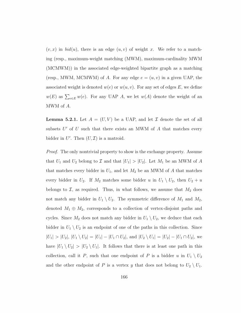
(v, x) in bid(u), there is an edge (u, v) of weight x. We refer to a match-

ing (resp., maximum-weight matching (MWM), maximum-cardinality MWM

(MCMWM)) in the associated edge-weighted bipartite graph as a matching

(resp., MWM, MCMWM) of A. For any edge e = (u, v) in a given UAP, the

associated weight is denoted w(e) or w(u, v). For any set of edges E, we define

w(E) as∑

e∈E w(e). For any UAP A, we let w(A) denote the weight of an

MWM of A.

Lemma 5.2.1. Let A = (U, V ) be a UAP, and let I denote the set of all

subsets U ′ of U such that there exists an MWM of A that matches every

bidder in U ′. Then (U, I) is a matroid.

Proof. The only nontrivial property to show is the exchange property. Assume

that U1 and U2 belong to I and that |U1| > |U2|. Let M1 be an MWM of A

that matches every bidder in U1, and let M2 be an MWM of A that matches

every bidder in U2. If M2 matches some bidder u in U1 \ U2, then U2 + u

belongs to I, as required. Thus, in what follows, we assume that M2 does

not match any bidder in U1 \ U2. The symmetric difference of M1 and M2,

denoted M1 ⊕ M2, corresponds to a collection of vertex-disjoint paths and

cycles. Since M2 does not match any bidder in U1 \ U2, we deduce that each

bidder in U1 \ U2 is an endpoint of one of the paths in this collection. Since

|U1| > |U2|, |U1 \ U2| = |U1| − |U1 ∩ U2|, and |U2 \ U1| = |U2| − |U1 ∩ U2|, we

have |U1 \ U2| > |U2 \ U1|. It follows that there is at least one path in this

collection, call it P , such that one endpoint of P is a bidder u in U1 \ U2

and the other endpoint of P is a vertex y that does not belong to U2 \ U1.

166

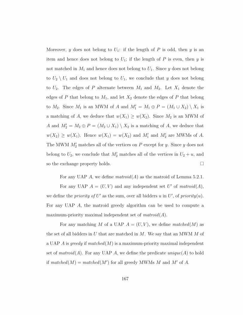
Moreover, y does not belong to U1: if the length of P is odd, then y is an

item and hence does not belong to U1; if the length of P is even, then y is

not matched in M1 and hence does not belong to U1. Since y does not belong

to U2 \ U1 and does not belong to U1, we conclude that y does not belong

to U2. The edges of P alternate between M1 and M2. Let X1 denote the

edges of P that belong to M1, and let X2 denote the edges of P that belong

to M2. Since M1 is an MWM of A and M ′1 = M1 ⊕ P = (M1 ∪ X2) \ X1 is

a matching of A, we deduce that w(X1) ≥ w(X2). Since M2 is an MWM of

A and M ′2 = M2 ⊕ P = (M2 ∪ X1) \ X2 is a matching of A, we deduce that

w(X2) ≥ w(X1). Hence w(X1) = w(X2) and M ′1 and M ′

2 are MWMs of A.

The MWM M ′2 matches all of the vertices on P except for y. Since y does not

belong to U2, we conclude that M ′2 matches all of the vertices in U2 + u, and

so the exchange property holds.

For any UAP A, we define matroid(A) as the matroid of Lemma 5.2.1.

For any UAP A = (U, V ) and any independent set U ′ of matroid(A),

we define the priority of U ′ as the sum, over all bidders u in U ′, of priority(u).

For any UAP A, the matroid greedy algorithm can be used to compute a

maximum-priority maximal independent set of matroid(A).

For any matching M of a UAP A = (U, V ), we define matched(M) as

the set of all bidders in U that are matched in M . We say that an MWM M of

a UAP A is greedy if matched(M) is a maximum-priority maximal independent

set of matroid(A). For any UAP A, we define the predicate unique(A) to hold

if matched(M) = matched(M ′) for all greedy MWMs M and M ′ of A.

167

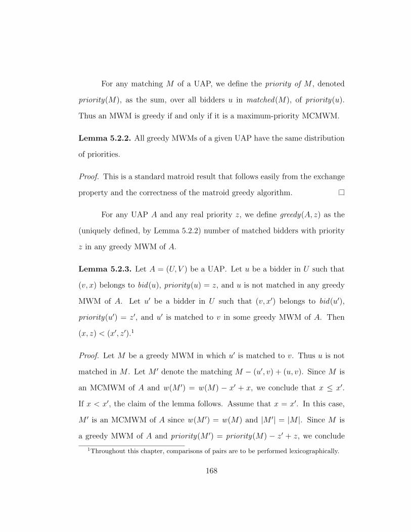
For any matching M of a UAP, we define the priority of M , denoted

priority(M), as the sum, over all bidders u in matched(M), of priority(u).

Thus an MWM is greedy if and only if it is a maximum-priority MCMWM.

Lemma 5.2.2. All greedy MWMs of a given UAP have the same distribution

of priorities.

Proof. This is a standard matroid result that follows easily from the exchange

property and the correctness of the matroid greedy algorithm.

For any UAP A and any real priority z, we define greedy(A, z) as the

(uniquely defined, by Lemma 5.2.2) number of matched bidders with priority

z in any greedy MWM of A.

Lemma 5.2.3. Let A = (U, V ) be a UAP. Let u be a bidder in U such that

(v, x) belongs to bid(u), priority(u) = z, and u is not matched in any greedy

MWM of A. Let u′ be a bidder in U such that (v, x′) belongs to bid(u′),

priority(u′) = z′, and u′ is matched to v in some greedy MWM of A. Then

(x, z) < (x′, z′).1

Proof. Let M be a greedy MWM in which u′ is matched to v. Thus u is not

matched in M . Let M ′ denote the matching M − (u′, v) + (u, v). Since M is

an MCMWM of A and w(M ′) = w(M) − x′ + x, we conclude that x ≤ x′.

If x < x′, the claim of the lemma follows. Assume that x = x′. In this case,

M ′ is an MCMWM of A since w(M ′) = w(M) and |M ′| = |M |. Since M is

a greedy MWM of A and priority(M ′) = priority(M) − z′ + z, we conclude

1Throughout this chapter, comparisons of pairs are to be performed lexicographically.

168

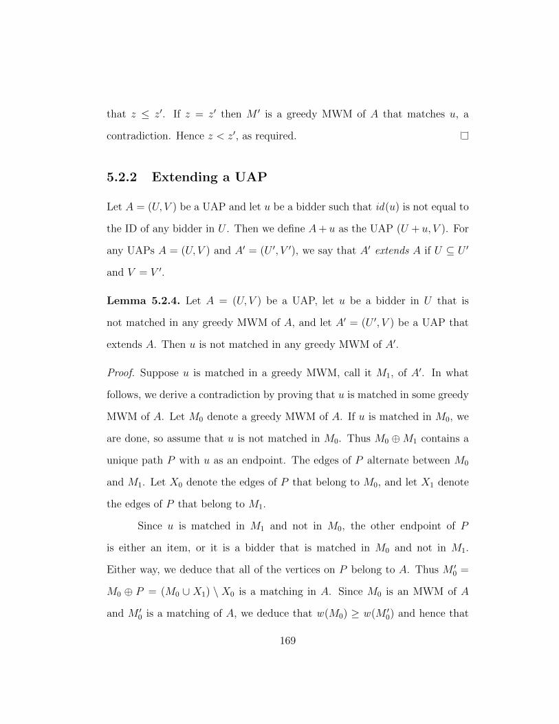
that z ≤ z′. If z = z′ then M ′ is a greedy MWM of A that matches u, a

contradiction. Hence z < z′, as required.

5.2.2 Extending a UAP

Let A = (U, V ) be a UAP and let u be a bidder such that id(u) is not equal to

the ID of any bidder in U . Then we define A+ u as the UAP (U + u, V ). For

any UAPs A = (U, V ) and A′ = (U ′, V ′), we say that A′ extends A if U ⊆ U ′

and V = V ′.

Lemma 5.2.4. Let A = (U, V ) be a UAP, let u be a bidder in U that is

not matched in any greedy MWM of A, and let A′ = (U ′, V ) be a UAP that

extends A. Then u is not matched in any greedy MWM of A′.

Proof. Suppose u is matched in a greedy MWM, call it M1, of A′. In what

follows, we derive a contradiction by proving that u is matched in some greedy

MWM of A. Let M0 denote a greedy MWM of A. If u is matched in M0, we

are done, so assume that u is not matched in M0. Thus M0 ⊕M1 contains a

unique path P with u as an endpoint. The edges of P alternate between M0

and M1. Let X0 denote the edges of P that belong to M0, and let X1 denote

the edges of P that belong to M1.

Since u is matched in M1 and not in M0, the other endpoint of P

is either an item, or it is a bidder that is matched in M0 and not in M1.

Either way, we deduce that all of the vertices on P belong to A. Thus M ′0 =

M0 ⊕ P = (M0 ∪ X1) \ X0 is a matching in A. Since M0 is an MWM of A

and M ′0 is a matching of A, we deduce that w(M0) ≥ w(M ′

0) and hence that

169

w(X0) ≥ w(X1). Since all of the vertices on P belong to A′, we conclude that

M ′1 = M1 ⊕ P = (M1 ∪X0) \X1 is a matching in A′. Since M1 is an MWM

of A′ and M ′1 is a matching of A′, we deduce that w(M1) ≥ w(M ′

1) and hence

that w(X1) ≥ w(X0). Thus w(X0) = w(X1), and we conclude that M ′0 is an

MWM of A.

Since u is matched in M1 and not in M0, we deduce that |X1| ≥ |X0|

and hence that |M ′0| ≥ |M0|. Since M0 is a greedy MWM of A, we know that

M0 is an MCMWM of A, and hence that |M0| ≥ |M ′0|. Thus |M0| = |M ′

0|

and hence |X0| = |X1| and M ′0 is an MCMWM of A. Since |X0| = |X1|, the

other endpoint of P is a bidder u′ that is matched in M0 and not in M1. Since

M0 is a greedy MWM of A and M ′0 is an MCMWM of A, we deduce that

priority(M0) ≥ priority(M ′0) and hence that priority(u′) ≥ priority(u).

Since |X0| = |X1| and w(X0) = w(X1), we deduce that M ′1 is an

MCMWM of A′. Since M1 is a greedy MWM of A′ and M ′1 is an MCMWM of

A′, we deduce that priority(M1) ≥ priority(M ′1) and hence that priority(u) ≥

priority(u′). Since we argued above that priority(u′) ≥ priority(u), we con-

clude that priority(u) = priority(u′), and hence that M ′0 is a greedy MWM of

A. This completes the proof, since u is matched in M ′0.

5.2.3 Finding a Greedy MWM

In this section, we briefly discuss how to efficiently compute a greedy MWM of

a UAP via a slight modification of the classic Hungarian method for the assign-

ment problem [39]. In the (maximization version of the) assignment problem,

170

we are given a set of n agents, a set of n tasks, and a weight for each agent-task

pair, and our objective is to find a perfect matching (i.e., every agent and task

is required to be matched) of maximum total weight. The Hungarian method

for the assignment problem proceeds as follows: a set of dual variables, namely

a “price” for each task, and a possibly incomplete matching are maintained; an

arbitrary unmatched agent u is chosen and a shortest augmenting path from u

to an unmatched task is computed using “residual costs” as the edge weights;

an augmentation is performed along the path to update the matching, and the

dual variables are adjusted in order to maintain complementary slackness; the

process repeats until a perfect matching is found.

Within our UAP setting, the set of bidders can be larger than the set of

items, and some bidder-item pairs may not be matchable, i.e., the associated

bipartite graph is not necessarily complete. In this setting, we can use an

“incremental” version of the Hungarian method to find an (not necessarily

greedy) MWM of a given UAP A = (U, V ) as follows. For the purpose of

simplifying the presentation of our method, we enlarge the set of items by

adding a dummy item v0 such that v0 is connected to each bidder u with an

edge of weight w(u, v0) = 0 and we always maintain v0 in the residual graph

with a price of 0. We start with the empty matching M . Then, for each bidder

u in U (in arbitrary order), we process u via an “incremental Hungarian step”

as follows: let U ′ denote the set of bidders that are matched by M ; let V ′

denote the set of items that are not matched by M ; find the shortest paths

from u to each item v in V ′ + v0 in the residual graph; let W denote the

171

minimum path weight among these shortest paths; choose a path P that is

either (1) a shortest path of weight W from u to an item v in V ′, or (2) a

shortest path from u to a bidder u′ in U ′ + u such that extending P with the

edge (u′, v0) yields a shortest path of weight W from u to v0; augment M along

P ; adjust the prices in order to maintain complementary slackness; update the

residual graph. The algorithm terminates when every non-reserve bidder has

been processed. The algorithm performs |U | incremental Hungarian steps and

each incremental Hungarian step can be implemented in O(|V | log |V | + m)

time by utilizing Fibonacci heaps [28], where m denotes the number of edges

in the residual graph, which is O(|V |2).

In order to find a greedy MWM, we slightly modify the implementation

described in the previous paragraph. Lemmas 5.2.7 and 5.2.8 established below

imply that choosing the path P in the following way results in a greedy MWM:

if a path of type (1) exists, we arbitrarily choose such a path; if no path

of type (1) exists, then we identify the nonempty set U ′′ of all bidders u′

such that a path of type (2) exists, and we choose a shortest path P that

terminates at a minimum priority bidder in U ′′. It is easy to see that the

described modification does not increase the asymptotic time complexity of

the algorithm. In the remainder of this section, we establish Lemmas 5.2.7,

5.2.8, and 5.2.9; Lemma 5.2.9 is used in Section 5.3.3 to prove Lemma 5.3.9.

We start with some useful definitions.

Let A = (U, V ) and A′ = A + u be UAPs, and let M be an MWM

of A. We define digraph(A, u,M) as the edge-weighted digraph that may

172

be obtained by modifying the subgraph of A induced by the set of vertices

(matched(M) + u) ∪ V as follows: for each edge that belongs to M , we direct

the edge from item to bidder and leave the weight unchanged; for each edge

that does not belong to M , we direct the edge from bidder to item and negate

the weight.

Lemma 5.2.5. Let A = (U, V ) and A′ = A + u be UAPs, let M be an

MWM of A, and let G denote digraph(A, u,M). Then G does not contain any

negative-weight cycles.

Proof. Such a cycle could not involve u (since u only has outgoing edges) so

it has to be a negative-weight cycle that already existed before u was added,

a contradiction since M is an MWM of A.

Let A = (U, V ) and A′ = A + u be UAPs, let M be an MWM of A,

and let G denote digraph(A, u,M). We define a set of items holes(A, u,M),

and a set of bidders candidates(A, u,M), as follows. By Lemma 5.2.5, the

shortest path distance in G from bidder u to any vertex reachable from u is

well-defined. We define holes(A, u,M) as the set of all items v in V such that

v is unmatched in M and the weight of a shortest path in G from u to v is

w(A)−w(A′). We define candidates(A, u,M) as the set of all bidders u′ such

that the weight of a shortest path in G from u to u′ is equal to w(A)−w(A′).

Let A = (U, V ) and A′ = A + u be UAPs, let M be an MWM of A,

and let P be a directed path in digraph(A, u,M) that starts at u, has weight

w(A)− w(A′), and terminates at either an item in holes(A, u,M) or a bidder

in candidates(A, u,M). (Note that P could be a path of length zero from u to

173

u.) Let X denote the edges in M that correspond to item-to-bidder edges in

P , and let Y denote the edges in A′ that correspond to bidder-to-item edges

in P . It is easy to see that the set of edges (M \ X) ∪ Y is an MWM of A′.

We define this MWM of A′ as augment(A, u,M, P ).

Lemma 5.2.6. Let A = (U, V ) be a UAP, let M be a greedy MWM of A, let u

be a bidder that does not belong to U , let A′ denote the UAP (U+u, V ), and let

M ′ denote a greedy MWM of A′ minimizing |M⊕M ′|. Then digraph(A, u,M)

contains a directed path P satisfying the following conditions: P has weight

w(A) − w(A′); P starts at u; the bidder-to-item edges in P correspond to

the edges in M ′ \M ; the item-to-bidder edges in P correspond to the edges

in M \M ′; if holes(A, u,M) is nonempty, then P terminates at an item in

holes(A, u,M); if holes(A, u,M) is empty, then P terminates at a minimum-

priority bidder in candidates(A, u,M).

Proof. The edges of M ⊕M ′ form a collection S of disjoint cycles and paths

of positive length.

We begin by arguing that S does not contain any cycles. Suppose there

is a cycle C in S. Let X denote the edges of C that belong to M \M ′, and let

Y denote the edges of C that belong to M ′ \M . Let M ′′ denote (M ∪Y ) \X,

which is a matching in A since u is unmatched in M and hence does not belong

to C. Since M is an MWM of A and w(M ′′) = w(M) + w(Y ) − w(X), we

conclude that w(X) ≥ w(Y ). Let M ′′′ denote (M ′∪X)\Y , which is a matching

in A′. Since M ′ is an MWM of A′ and w(M ′′′) = w(M ′) + w(Y )− w(X), we

conclude that w(X) ≤ w(Y ). Thus w(X) = w(Y ) and hence w(M ′′′) =

174

w(M ′), implying that M ′′′ is an MWM of A′. Moreover, since M ′′′ matches

the same set of bidders as M ′, we find that M ′′′ is a greedy MWM of A′. This

contradicts the definition of M ′ since |M ⊕M ′′′| < |M ⊕M ′|.

Next we argue that if Q is a path in S, then u is an endpoint of Q.

Suppose there is a path Q in S such that u is not an endpoint of Q. Thus u

does not appear on Q since u is unmatched in M . Let X denote the edges of Q

that belong to M \M ′, and let Y denote the edges of Q that belong to M ′\M .

Let M ′′ denote (M ∪Y )\X, which is a matching in A since u does not belong

to Q. Since M is an MWM of A and w(M ′′) = w(M) + w(Y ) − w(X), we

conclude that w(X) ≥ w(Y ). Let M ′′′ denote (M ′∪X)\Y , which is a matching

in A′. Since M ′ is an MWM of A′ and w(M ′′′) = w(M ′) + w(Y )− w(X), we

conclude that w(X) ≤ w(Y ). Thus w(X) = w(Y ) and hence w(M ′′) = w(M)

and w(M ′′′) = w(M ′), implying that M ′′ is an MWM of A and M ′′′ is an

MWM of A′. Since M is a greedy MWM and hence an MCMWM of A, the

set of bidders matched by M is not properly contained in the set of bidders

matched by M ′′; we conclude that |X| ≥ |Y |. Since M ′ is a greedy MWM and

hence an MCMWM of A′, the set of bidders matched by M ′ is not properly

contained in the set of bidders matched by M ′′′; we conclude that |X| ≤ |Y |.

Thus |X| = |Y |, so the length of path Q is even. We consider two cases.

Case 1: The endpoints of Q are items. In this case, M ′ and M ′′′

match the same set of bidders, and hence M ′′′ is a greedy MWM of A′.

This contradicts the definition of M ′, since Q has positive length and hence

|M ⊕M ′′′| < |M ⊕M ′|.

175

Case 2: The endpoints ofQ are bidders. SinceQ has positive length, one

endpoint, call it u0, is matched in M but not in M ′, and the other endpoint,

call it u1, is matched in M ′ but not in M . Since M is a greedy MWM of

A and M ′′ is an MWM of A, we deduce that priority(u0) ≥ priority(u1).

Since M ′ is a greedy MWM of A′ and M ′′′ is an MWM of A′, we deduce

that priority(u0) ≤ priority(u1). Thus priority(u0) = priority(u1). It follows

that priority(M ′′′) = priority(M ′). Hence M ′′′ is a greedy MWM of A′. This

contradicts the definition of M ′ since |M ⊕M ′′′| < |M ⊕M ′|.

From the preceding arguments, we deduce that either M = M ′ or M ⊕

M ′ corresponds to a positive-length path with u as an endpoint. Equivalently,

M⊕M ′ is the edge set of a path that has u as an endpoint and may have length

zero (i.e., the path may begin and end at u). We claim if the edges of this path

are directed away from endpoint u, we obtain a directed path P satisfying the

six conditions stated in the lemma. It is easy to see that P satisfies the first

four of these conditions. It remains to establish that P satisfies the fifth and

sixth conditions.

For the fifth condition, assume that holes(A, u,M) is nonempty. We

need to prove that P terminates at an item in holes(A, u,M). Since

holes(A, u,M) is nonempty, we deduce that |M ′| = |M | + 1, and hence that

P terminates at some item v. Since P has weight w(A) − w(A′), we deduce

that v belongs to holes(A, u,M), as required.

For the sixth condition, assume that holes(A, u,M) is empty. We need

to prove that P terminates at a minimum-priority bidder in candidates(A, u,M).

176

Suppose P terminates at some item v. Since P has weight w(A) − w(A′),

we deduce that v belongs to holes(A, u,M), a contradiction. Thus P ter-

minates at some bidder u′. Since P has weight w(A) − w(A′), we deduce

that u′ belongs to candidates(A, u,M). If u′ is not a minimum-priority bid-

der in candidates(A, u,M), it is easy to argue that M ′ is not a greedy MWM

of A′, a contradiction. Thus P terminates at a minimum-priority bidder in

candidates(A, u,M).

Lemma 5.2.7. Let A = (U, V ) be a UAP, let M be a greedy MWM of A, let

u be a bidder that does not belong to U , let A′ denote the UAP (U + u, V ),

let P be a directed path in digraph(A, u,M) of weight w(A) − w(A′) from u

to an item in holes(A, u,M), and let M∗ denote augment(A, u,M, P ). Then

M∗ is a greedy MWM of A′.

Proof. The definition of augment(A, u,M, P ) implies that M∗ is an MWM of

A′. Let M ′ denote a greedy MWM of A′ minimizing |M ⊕M ′|. Let U ′ denote

the set of bidders in A matched by M . Since holes(A, u,M) is nonempty,

Lemma 5.2.6 implies that the set of bidders in A′ matched by M ′ is U ′ + u.

Since M∗ is an MWM of A′ that also matches the set of bidders U ′ + u, we

deduce that M∗ is a greedy MWM of A′.

Lemma 5.2.8. Let A = (U, V ) be a UAP, let M be a greedy MWM of A,

let u be a bidder that does not belong to U , and let A′ denote the UAP

(U + u, V ). Assume that holes(A, u,M) is empty. Let u′ denote a minimum-

priority bidder in candidates(A, u,M) (which is nonempty by Lemma 5.2.6),

let P be a directed path in digraph(A, u,M) of weight w(A) − w(A′) from u

177

to u′, and let M∗ denote augment(A, u,M, P ). Then M∗ is a greedy MWM of

A′.

Proof. The definition of augment(A, u,M, P ) implies that M∗ is an MWM

of A′. Let M ′ denote a greedy MWM of A′ minimizing |M ⊕M ′|. Let U ′

denote the set of bidders in A matched by M . Since holes(A, u,M) is empty,

Lemma 5.2.6 implies that the set of bidders in A′ matched by M ′ is U ′ + u−

u′′, where u′′ is some minimum-priority bidder in candidates(A, u,M). It is

straightforward to check that M∗ has the same weight, cardinality, and priority

as M ′. Thus M∗ is a greedy MWM of A′, as required.

Lemma 5.2.9. Let A and A′ be two UAPs such that A′ extends A, let M be

a greedy MWM of A, and let M ′ be a greedy MWM of A′. Then |M ′| ≥ |M |.

Proof. Immediate from Lemmas 5.2.7 and 5.2.8.

5.2.4 Threshold of an Item

In this section, we define the notion of a “threshold” of an item in a UAP.

This lays the groundwork for a corresponding IUAP definition in Section 5.3.3.

Item thresholds play an important role in our strategyproofness results.

Lemma 5.2.10. Let A = (U, V ) be a UAP and let v be an item in V . Let

U ′ be the set of bidders u such that A+ u is a UAP and bid(u) is of the form

(v, x). Then there is a unique pair of reals (x∗, z∗) such that for any bidder

u in U ′, the following conditions hold, where A′ denotes A + u, x denotes

w(u, v), and z denotes priority(u): (1) if (x, z) > (x∗, z∗) then u is matched

178

in every greedy MWM of A′; (2) if (x, z) < (x∗, z∗) then u is not matched in

any greedy MWM of A′; (3) if (x, z) = (x∗, z∗) then u is matched in some but

not all greedy MWMs of A′.

Proof. Let M be a greedy MWM of A, let W denote w(M), and let Z denote

priority(M). LetM denote the set of matchings of A′ that do not match v, let

M′ denote the maximum-weight elements ofM, letM′′ denote the maximum-

cardinality elements ofM′, letM′′′ denote the maximum-priority elements of

M′′, and observe that there is a unique pair of reals (W ′, Z ′) such that any

matching M ′ in M′′′ has weight W ′ and priority Z ′. It is straightforward to

verify that the unique choice of (x∗, z∗) satisfying the conditions stated in the

lemma is (W −W ′, Z − Z ′).

For any UAP A = (U, V ) and any item v in V , we define the unique

pair (x∗, z∗) of Lemma 5.2.10 as threshold(A, v).

5.3 Iterated Unit-Demand Auctions with Pri-

orities

In this section, we formally define the notion of an iterated unit-demand auc-

tion with priorities (IUAP). An IUAP allows the bidders, called “multibid-

ders” in this context, to have a sequence of unit-demand bids instead of a

single unit-demand bid. In Section 5.3.1, we define a mapping from an IUAP

to a UAP by describing an algorithm that generalizes the DA algorithm, and

we establish Lemma 5.3.5 that is useful for analyzing the matching produced

179

by Algorithm 5.2 of Section 5.4. Lemma 5.3.5 is used to establish weak sta-

bility (Lemmas 5.4.1, 5.4.2, and 5.4.3) and Pareto-optimality (Lemma 5.4.4).

In Section 5.3.3, we define the threshold of an item in an IUAP and we estab-

lish Lemma 5.3.8, which plays a key role in establishing our strategyproofness

results. We start with some useful definitions.

A multibidder t for a set of items V is a pair (σ, z) where z is a real

priority and σ is a sequence of bidders for V such that all the bidders in

σ have distinct IDs and a common priority z. We define priority(t) as z.

For any integer i such that 1 ≤ i ≤ |σ|, we define bidder(t, i) as the bidder

σ(i). For any integer i such that 0 ≤ i ≤ |σ|, we define bidders(t, i) as

bidder(t, j) | 1 ≤ j ≤ i. We define bidders(t) as bidders(t, |σ|).

An iterated UAP (IUAP) is a pair B = (T, V ) where V is a set of items

and T is a set of multibidders for V . In addition, for any distinct multibidders

t and t′ in T , the following conditions hold: priority(t) 6= priority(t′); if u

belongs to bidders(t) and u′ belongs to bidders(t′), then id(u) 6= id(u′). For

any IUAP B = (T, V ), we define bidders(B) as the union, over all t in T , of

bidders(t).

5.3.1 Mapping an IUAP to a UAP

Having defined the notion of an IUAP, we now describe an algorithm that maps

a given IUAP to a UAP. Our algorithm generalizes the DA algorithm. In each

iteration of the DA algorithm, an arbitrary single man is chosen, and this

man reveals his next choice. In each iteration of our algorithm, an arbitrary

180

single multibidder is chosen, and this multibidder reveals its next bid. We

prove in Lemma 5.3.4 that, like the DA algorithm, our algorithm is confluent:

the output does not depend on the nondeterministic choices made during an

execution. We conclude this section by establishing Lemma 5.3.5, which is

useful for analyzing the matching produced by Algorithm 5.2 in Section 5.4.1.

Lemma 5.3.5 is used to establish weak stability (Lemmas 5.4.1, 5.4.2, and 5.4.3)

and Pareto-optimality (Lemma 5.4.4). We start with some useful definitions.

Let A be a UAP (U, V ) and let B be an IUAP (T, V ). The predicate

prefix (A,B) is said to hold if U ⊆ bidders(B) and for any multibidder t in T ,

U ∩ bidders(t) = bidders(t, i) for some i.

A configuration C is a pair (A,B) where A is a UAP, B is an IUAP,

and prefix (A,B) holds.

Let C = (A,B) be a configuration, where A = (U, V ) and B = (T, V ),

and let u be a bidder in U . Then we define multibidder(C, u) as the unique

multibidder t in T such that u belongs to bidders(t).

Let C = (A,B) be a configuration where A = (U, V ) and B = (T, V ).

For any t in T , we define bidders(C, t) as u ∈ U | multibidder(C, u) = t.

Let C = (A,B) be a configuration where B = (T, V ). We define

ready(C) as the set of all bidders u in bidders(B) such that greedy(A, priority(u))

= 0 and u = bidder(t, |bidders(C, t)|+ 1) where t = multibidder(C, u).

Our algorithm for mapping an IUAP to a UAP is Algorithm 5.1. The

input is an IUAP B and the output is a UAP A such that prefix (A,B) holds.

The algorithm starts with the UAP consisting of all the items in V but no

181

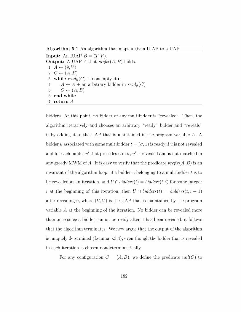
Algorithm 5.1 An algorithm that maps a given IUAP to a UAP.

Input: An IUAP B = (T, V ).Output: A UAP A that prefix (A,B) holds.

1: A← (∅, V )2: C ← (A,B)3: while ready(C) is nonempty do4: A← A + an arbitrary bidder in ready(C)5: C ← (A,B)6: end while7: return A

bidders. At this point, no bidder of any multibidder is “revealed”. Then, the

algorithm iteratively and chooses an arbitrary “ready” bidder and “reveals”

it by adding it to the UAP that is maintained in the program variable A. A

bidder u associated with some multibidder t = (σ, z) is ready if u is not revealed

and for each bidder u′ that precedes u in σ, u′ is revealed and is not matched in

any greedy MWM of A. It is easy to verify that the predicate prefix (A,B) is an

invariant of the algorithm loop: if a bidder u belonging to a multibidder t is to

be revealed at an iteration, and U ∩ bidders(t) = bidders(t, i) for some integer

i at the beginning of this iteration, then U ∩ bidders(t) = bidders(t, i + 1)

after revealing u, where (U, V ) is the UAP that is maintained by the program

variable A at the beginning of the iteration. No bidder can be revealed more

than once since a bidder cannot be ready after it has been revealed; it follows

that the algorithm terminates. We now argue that the output of the algorithm

is uniquely determined (Lemma 5.3.4), even though the bidder that is revealed

in each iteration is chosen nondeterministically.

For any configuration C = (A,B), we define the predicate tail(C) to

182

hold if for any bidder u that is matched in some greedy MWM of A, we have

u = bidder(t, |bidders(C, t)|) where t denotes multibidder(C, u).

Lemma 5.3.1. Let C = (A,B) be a configuration where B = (T, V ) and

assume that tail(C) holds. Then greedy(A, priority(t)) ≤ 1 for each t in T .

Proof. The claim of the lemma easily follows from the definition of tail(C).

Lemma 5.3.2. The predicate tail(C) is an invariant of the Algorithm 5.1

loop.

Proof. It is easy to see that tail(C) holds when the loop is first encountered.

Now consider an iteration of the loop that takes us from configuration C =

(A,B) where A = (U, V ) to configuration C ′ = (A′, B) where A′ = (U ′, V ).

We need to show that tail(C ′) holds. Let u be a bidder that is matched in

some greedy MWM M ′ of A′. Let u∗ denote the bidder that is added to A in

line 4, and consider the following three cases.

Case 1: u = u∗. Let t denote multibidder(C ′, u∗). In this case,

|bidders(C, t)| + 1 = |bidders(C ′, t)|, so u∗ = bidder(t, |bidders(C ′, t)|), as re-

quired.

Case 2: u 6= u∗ and priority(u) 6= priority(u∗). Since U ′ contains U ,

Lemma 5.2.4 implies that u is matched in some greedy MWM of A. Since C is

a configuration and tail(C) holds, we deduce that u = bidder(t, |bidders(C, t)|)

where t denotes multibidder(C, u). Since multibidder(C ′, u) = multibidder(C, u)

and bidders(C ′, t) = bidders(C, t), we conclude that u = bidder(t, |bidders(C ′, t)|),

where t denotes multibidder(C ′, u), as required.

183

Case 3: u 6= u∗ and priority(u) = priority(u∗). Since u∗ belongs to

ready(C), we know that greedy(A, priority(u)) = 0. Also, since u is not u∗, u

belongs to U and we conclude that u is not matched in any greedy MWM of

A. Since U ′ contains U , Lemma 5.2.4 implies that u is not matched in any

greedy MWM of A′, a contradiction.

Lemma 5.3.3. Let C = (A,B) be a configuration such that tail(C) holds.

Then unique(A) holds.

Proof. Let M and M ′ be greedy MWMs of A, and let u be a bidder in

matched(M). To establish the lemma, it is sufficient to prove that u belongs

to matched(M ′). Let t denote multibidder(C, u) and let z denote priority(t).

Since tail(C) holds, we know that u = bidder(t, |bidders(C, t)|). Since u is

matched byM and since tail(C) holds, Lemma 5.3.1 implies that greedy(A, z) =

1. Thus Lemma 5.2.2 implies that M ′ matches one priority-z bidder. Since

tail(C) holds, this bidder is u.

Lemma 5.3.4. Let B = (T, V ) be an IUAP. Then all executions of Algo-

rithm 5.1 on input B produce the same output.

Proof. Suppose not, and let X1 and X2 denote two executions of Algorithm 5.1

on input B that produce distinct output UAPs A1 = (U1, V ) and A2 = (U2, V ).

Without loss of generality, assume that |U1| ≥ |U2|. Then there is a first

iteration of execution X1 in which the bidder added to A in line 4 belongs to

U1 \U2; let u′ denote this bidder. Let C ′ = (A′, B) where A′ = (U ′, V ) denote

the configuration in program variable C at the start of this iteration, and let

184

t′ denote multibidder(C ′, u′). Let i be the integer such that u′ = bidder(t′, i).

We know that i > 1 because it is easy to see that U2 contains bidder(t′, 1).

Let u′′ denote bidder(t′, i − 1). Since u′ belongs to ready(C ′), Lemmas 5.3.2

and 5.3.3 imply that u′′ is not matched in any greedy MWM of A′. Since U ′

is contained in U2, Lemma 5.2.4 implies that u′′ is not matched in any greedy

MWM of A2. Let C2 = (A2, B) denote the final configuration of execution

X2; thus ready(C2) is empty and |bidders(C2, t′)| = i − 1. By Lemma 5.3.2,

we conclude that greedy(A2, priority(t′)) = 0, and hence that u′′ is contained

in ready(C2), a contradiction.

For any IUAP B, we define uap(B) as the unique (by Lemma 5.3.4)

UAP returned by any execution of Algorithm 5.1 on input B.

We now present a lemma that is used in Section 5.4 to establish weak

stability (Lemmas 5.4.1, 5.4.2, and 5.4.3) and Pareto-optimality (Lemma 5.4.4).

Lemma 5.3.5. Let B = (T, V ) be an IUAP, let (σ, z) be a multibidder that

belongs to T , let uap(B) be (U, V ), and let M be a greedy MWM of the UAP

(U, V ). Then the following claims hold: (1) if σ(k) is matched in M for some

k, then σ(k′) ∈ U if and only if 1 ≤ k′ ≤ k; (2) if σ(k) is not matched in M

for any k, then σ(k) ∈ U for 1 ≤ k ≤ |σ|.

Proof. Since prefix (A,B) and tail(C) hold at the end of Algorithm 5.1 by

Lemma 5.3.2, the first claim follows. Since ready(C) is empty at the end of

Algorithm 5.1, the second claim follows.

185

5.3.2 Hungarian-Based Implementation of Algorithm 5.1

In this section, we briefly discuss how to implement Algorithm 5.1 efficiently

and how to compute a greedy MWM of uap(B) by maintaining a greedy

MWM of the UAP A. We use the modified incremental Hungarian step of

Section 5.2.3 in each iteration of the loop of Algorithm 5.1 to maintain A and

a greedy MWM of A, as follows: we maintain dual variables (a price for each

item) and a residual graph; the initial greedy MWM is the empty matching;

when a bidder u is added to A at line 4, we perform an incremental Hungarian

step to process u to update the greedy MWM, the prices, and the residual

graph. Since we maintain a greedy MWM of A at each iteration of the loop, it

is easy to see that identifying a bidder in ready(C) (or determining that this set

is empty) takes O(|V |) time. Thus the whole algorithm can be implemented

in O(|bidders(B)| · |V |2) time.

5.3.3 Threshold of an Item

In this section, we define the threshold of an item in an IUAP and we establish

Lemma 5.3.8, which plays a key role in establishing our strategyproofness

results. We start with some useful definitions.

For any IUAP B, Lemmas 5.3.2 and 5.3.3 imply that unique(uap(B))

holds, and thus that every greedy MWM of uap(B) matches the same set of

bidders. We define this set of matched bidders as winners(B). For any IUAP

B, we define losers(B) as U \ winners(B) where (U, V ) is uap(B).

Let B = (T, V ) be an IUAP and let u = (α, β, z) be a bidder for V .

186

Then we define the IUAP B + u as follows: if T contains a multibidder t

of the form (σ, z) for some sequence of bidders σ, then we define B + u as

(T − t+ t′, V ) where t′ = (σ′, z) and σ′ is the sequence of bidders obtained by

appending u to σ; otherwise, we define B + u as (T + t, V ) where t = (〈u〉, z).

Lemma 5.3.6. Let B = (T, V ) and B′ = B+u be IUAPs. Then losers(B) ⊆

losers(B′).

Proof. Let u′ be a bidder in losers(B). Thus u′ is not matched in any greedy

MWM of uap(B). Using Lemma 5.3.4, it is easy to see that uap(B′) extends

uap(B). Thus Lemma 5.2.4 implies that u′ is not matched in any greedy

MWM of uap(B′), and hence that u′ belongs to losers(B′).

Lemma 5.3.7. Let B = (T, V ) be an IUAP and let v be an item in V . For

i ∈ 1, 2, let Bi = B + ui be an IUAP where ui = (αi, (v, xi) , zi). Let

A1 = (U1, V ) denote uap(B1) and let A2 = (U2, V ) denote uap(B2). Assume

that α1 6= α2, z1 6= z2, and u1 belongs to winners(B1). Then the following

claims hold: if u2 belongs to winners(B2) then U1−u1 = U2−u2; if u2 belongs

to losers(B2) then U1 − u1 contains U2 − u2.

Proof. Let B3 denote the IUAP B1 + u2, which is equal to B2 + u1. For the

first claim, assume that u2 belongs to winners(B2). Using Lemma 5.3.4, it is

straightforward to argue that uap(B3) is equal to A1 + u2 = (U1 + u2, V ) and

is also equal to A2 + u1 = (U2 + u1, V ). Since u1 belongs to U1 and u2 belongs

to U2, we conclude that U1 − u1 = U2 − u2, as required.

For the second claim, assume that u2 belongs to losers(B2). Suppose

(x1, z1) < (x2, z2). Then Lemmas 5.2.3 and 5.3.4 imply that u2 belongs to

187

winners(B3). Since u2 belongs to losers(B2), Lemma 5.3.6 implies that u2

belongs to losers(B2 + u1) = losers(B3), a contradiction. Since z1 6= z2, we

conclude that (x1, z1) > (x2, z2). Then, Lemma 5.3.4 implies that uap(B3) =

uap(B1) + u2 = (U1 + u2, V ). Since Lemma 5.3.4 also implies that uap(B3)

extends uap(B2), it follows that U1+u2 contains U2, and hence that U1 contains

U2 − u2. Since u1 does not belong to U2, we conclude that U1 − u1 contains

U2 − u2, as required.

We are now ready to define the threshold of an item in an IUAP, and

to state Lemma 5.3.8. In Section 5.4, Lemma 5.3.8 plays an important role in

establishing that our SMIW mechanism is strategyproof (Lemma 5.4.6). The

proof of Lemma 5.3.8 is provided in Section 5.3.3.

Let B = (T, V ) be an IUAP and let v be an item in V . By Lemma 5.3.7,

there is a unique subset U of bidders(B) such that the following condition

holds: for any IUAP B′ = B + u where u is of the form (α, (v, x) , z) and u

belongs to winners(B′), uap(B′) is equal to (U + u, V ). We define uap(B, v)

as the UAP (U, V ), and we define threshold(B, v) as threshold(uap(B, v), v).

Lemma 5.3.8. Let B = (T, V ) be an IUAP, let t = (σ, z) be a multibidder

that belongs to T , and let B′ denote the IUAP (T − t, V ). Suppose that

(σ(k), v) is matched in some greedy MWM of uap(B) for some k. Then

(w(σ(k), v), z) ≥ threshold(B′, v). (5.1)

Furthermore, for each k′ and v′ such that 1 ≤ k′ < k and v′ belongs to

188

items(σ(k′)), we have

(w(σ(k′), v′), z) < threshold(B′, v′). (5.2)

Proof of Lemma 5.3.8

The purpose of this section is to prove Lemma 5.3.8. We do so by establishing a

stronger result, namely Lemma 5.3.16 below. We start with a useful definition.

For any IUAP B, we define priorities(B) as z | u ∈ winners(B) and

priority(u) = z.

Lemma 5.3.9. Let B = (T, V ) and B′ = B + u = (T ′, V ) be IUAPs, let Z

denote priorities(B), let Z ′ denote priorities(B′), and let z denote priority(u).

Then |Z ′| ≥ |Z| and Z ′ ⊆ Z + z.

Proof. Consider running Algorithm 5.1 on input B′, where we avoid select-

ing bidder u from ready(C) unless it is the only bidder in ready(C). (By

Lemma 5.3.4, the final output is the same regardless of which bidder is se-

lected from ready(C) at each iteration.) If u never enters ready(C), then

uap(B′) = uap(B), and so Z ′ = Z, and the claim of the lemma holds.

Now suppose that u enters ready(C) at some point. Let A = (U, V )

denote the UAP at the start of the iteration in which u is selected from

ready(C). Then A is equal to uap(B), and we deduce that uap(B′) extends

uap(B). Lemma 5.3.1 implies that every greedy MWM of A = uap(B) (resp.,

uap(B′)) matches exactly one bidder of each priority in Z (resp., Z ′). Then,

since uap(B′) extends uap(B), Lemma 5.2.9 implies that |Z ′| ≥ |Z|. Fur-

189

thermore, letting U ′ denote the set of all bidders u′ in bidders(B) such that

priority(u′) does not belong to Z + z, we deduce that U ′ is contained in

losers(B) = U \ winners(B). Then Lemma 5.3.6 implies that no bidder in

U ′ is matched in any greedy MWM of uap(B′), and thus Z ′ ⊆ Z + z.

Lemma 5.3.10. Let A = (U, V ) and A′ = A + u be UAPs, and let v be an

item in V . Then threshold(A, v) ≤ threshold(A′, v).

Proof. Assume for the sake of contradiction that threshold(A, v) > threshold(A′, v).

Then there exists a bidder u′ such that u′ does not belong to U + u, bid(u′) =

(v, x) , priority(u′) = z, and

threshold(A′, v) < (x, z) < threshold(A, v).

Since (x, z) < threshold(A, v), Lemma 5.2.10 implies that u′ is not matched in

any greedy MWM of A+u′. Thus Lemma 5.2.4 implies that u′ is not matched

in any greedy MWM of A′ + u′. On the other hand, since threshold(A′, v) <

(x, z), Lemma 5.2.10 implies that u′ is matched in every greedy MWM of

A′ + u′, a contradiction.

Lemma 5.3.11. Let B = (T, V ) and B′ = B + u be IUAPs where u =

(α, (v, x) , z), v is an item in V , and z does not belong to priorities(B).

If u belongs to winners(B′), then (x, z) > threshold(B, v). If u belongs to

losers(B′), then (x, z) < threshold(B, v).

Proof. First, assume that u belongs to winners(B′). Thus u is matched in

every greedy MWM of uap(B′), which is equal to uap(B, v) + u by definition.

190

Lemma 5.2.10 implies that (x, z) > threshold(uap(B, v), v) = threshold(B, v),

as required.

Now assume that u belongs to losers(B′). Thus u is not matched in any

greedy MWM of uap(B′). Define U so that uap(B′) = (U + u, V ), and let A

denote the UAP (U, V ). Lemma 5.2.10 implies that (x, z) < threshold(A, v).

Lemma 5.3.7 implies that uap(B, v) + u extends uap(B′), and hence that

uap(B, v) extends A. Lemma 5.3.10 therefore implies that

threshold(A, v) ≤ threshold(uap(B, v), v) = threshold(B, v).

Thus (x, z) < threshold(B, v), as required.

Lemma 5.3.12. Let B = (T, V ) and B′ = B + u be IUAPs, and let v be an

item in V . Then threshold(B, v) ≤ threshold(B′, v).

Proof. Let (x, z) denote threshold(B, v), let (x′, z′) denote threshold(B′, v),

and assume for the sake of contradiction that (x, z) > (x′, z′).

Let u′ be a bidder (α, (v, x) , z′′) such that z′′ does not belong to

priorities(B)+priority(u), z > z′′, and (x, z′′) > (x′, z′). Let B′′ denote B+u′

and let B′′′ denote B′+u′. Since z′′ does not belong to priorities(B), we deduce

that u′ belongs to either winners(B′′) or losers(B′′). Then, by Lemma 5.3.11,

u′ belongs to losers(B′′), and hence by Lemma 5.3.6, u′ belongs to losers(B′′′).

On the other hand, since z′′ does not belong to priorities(B) + priority(u),

Lemma 5.3.9 implies that z′′ does not belong to priorities(B′), and we deduce

that u′ belongs to either winners(B′′′) or losers(B′′′). Then, Lemma 5.3.11

191

implies that u′ belongs to winners(B′′′), a contradiction.

Lemma 5.3.13. Let B = (T, V ) and B′ = B+u be IUAPs where u belongs to

losers(B′), and let v be an item in V . Then threshold(B′, v) = threshold(B, v).

Proof. Suppose not. Then by Lemma 5.3.12, we have threshold(B, v) <

threshold(B′, v). Let z denote priority(u). Since B′ = B + u and u be-

longs to losers(B′), we deduce that z does not belong to priorities(B). Since

u belongs to losers(B′), we deduce that z does not belong to priorities(B′).

Hence Lemma 5.3.9 implies that priorities(B′) = priorities(B).

Let B′′ denote B + u′ where u′ = (α, (v, x′) , z′) is a bidder such

that z′ does not belong to priorities(B) + z and threshold(B, v) < (x′, z′) <

threshold(B′, v).

Let B′′′ denote B′ + u′. Since z′ does not belong to priorities(B) + z,

Lemma 5.3.9 implies that z′ does not belong to priorities(B′), and we de-

duce that u′ belongs to either winners(B′′′) or losers(B′′′). Since (x′, z′) <

threshold(B′, v), Lemma 5.3.11 implies that u′ belongs to losers(B′′′). Hence

Lemma 5.3.9 implies that priorities(B′′′) = priorities(B′). Since we have es-

tablished above that priorities(B′) = priorities(B), we deduce that priorities(B′′′)

= priorities(B).

Since z′ does not belong to priorities(B), we deduce that u′ belongs to

either winners(B′′) or losers(B′′). Since (x′, z′) > threshold(B, v), Lemma 5.3.11

implies that u′ belongs to winners(B′′) and hence z′ belongs to priorities(B′′).

We consider two cases.

Case 1: |priorities(B′′)| ≤ |priorities(B)|. Lemma 5.3.9 implies that

192

there exists a real z′′ in priorities(B) that does not belong to priorities(B′′).

Since z does not belong to priorities(B), we have z 6= z′′. Since B′′′ = B′′ + u

and z 6= z′′, Lemma 5.3.9 implies that z′′ does not belong to priorities(B′′′), a

contradiction since priorities(B′′′) = priorities(B).

Case 2: |priorities(B′′)| > |priorities(B)|. Since priorities(B′′′) =

priorities(B), we deduce that |priorities(B′′)| > |priorities(B′′′)|. Since B′′′ =

B′′ + u, Lemma 5.3.9 implies that |priorities(B′′′)| ≥ |priorities(B′′)|, a con-

tradiction.

Lemma 5.3.14. Let B = (T, V ) and B′ = B+u be IUAPs where u = (α, β, z)

and z does not belong to priorities(B), and let v be an item in V . Assume

that (v, x) belongs to β, and that threshold(B, v) < (x, z). Then u belongs to

winners(B′).

Proof. Suppose not. Let A′ = (U ′, V ) denote uap(B′). Since z does not

belong to priorities(B), we deduce that u belongs to U ′. Thus u belongs to

U ′ \ winners(B′) = losers(B′), and so threshold(B′, v) = threshold(B, v) by

Lemma 5.3.13.

Let B′′ denote B′ + u′ where u′ = (α, (v, x) , z′) is a bidder such that

z′ does not belong to priorities(B) + z, threshold(B, v) < (x, z′), and z′ < z.

Since z′ does not belong to priorities(B) + z, we deduce that u′ belongs to

either winners(B′′) or losers(B′′). Then, by Lemma 5.3.11, u′ belongs to

winners(B′′). Let A′′ = (U ′′, V ) denote uap(B′′), and let M be a greedy

MWM of A′′. Since u′ belongs to winners(B′′), the edge (u′, v) belongs to

M . Since u belongs to losers(B′), Lemma 5.3.6 implies that u belongs to

193

losers(B′′), and hence that u is unmatched in M . By Lemma 5.2.3, we find

that (x, z) < (x, z′) and hence z < z′, a contradiction.

Lemma 5.3.15. Let B = (T, V ) and B0 = B + u be IUAPs where u =

(α, β, z), z does not belong to priorities(B), and β = (v1, x1), . . . , (vk, xk).

Assume that (xi, z) < threshold(B, vi) holds for all i such that 1 ≤ i ≤ k.

Then u belongs to losers(B0).

Proof. Suppose not. Since z does not belong to priorities(B), we deduce that

u belongs to winners(B0), and hence that z belongs to priorities(B0).

For i ranging from 1 to k, let Bi denote the IUAP Bi−1 +ui where ui =

(αi, (vi, xi) , zi) and zi is a real number satisfying the following conditions:

zi does not belong to priorities(Bi−1); z < zi; (xi, zi) < threshold(B, vi). Since

zi does not belong to priorities(Bi−1), we deduce that ui belongs to either

winners(Bi) or losers(Bi) for 1 ≤ i ≤ k. Then, by Lemmas 5.3.11 and 5.3.12,

we deduce that ui belongs to losers(Bi) for 1 ≤ i ≤ k. By repeated application

of Lemma 5.3.9, we find that priorities(Bi) = priorities(B0) for 1 ≤ i ≤ k,

and hence that z belongs to priorities(Bk).

We claim that u belongs to winners(Bk). To prove this claim, let t

denote the unique multibidder in Bk for which priority(t) = priority(u). Let

` denote |bidders(t)|, and observe that u = bidder(t, `). Furthermore, since

z does not belong to priorities(B), we deduce that bidder(t, i) belongs to

losers(B) for 1 ≤ i < `. By repeated application of Lemma 5.3.6, we deduce

that bidder(t, i) belongs to losers(Bk) for 1 ≤ i < `. Since z belongs to

priorities(Bk), the claim follows.

194

LetM denote a greedy MWM of uap(Bk). Since u belongs to winners(Bk),

there is a unique integer i, 1 ≤ i ≤ k, such that M contains edge (u, vi). Let i

denote this integer. Since zi does not belong to priorities(Bk), we know that

ui belongs to losers(Bk) and hence that ui is not matched in any greedy MWM

of uap(Bk). By Lemma 5.2.3, we deduce that (xi, zi) < (xi, z). Hence zi < z,

contradicting the definition of zi.

Lemma 5.3.16. Let B0 = (T, V ) be an IUAP, let z be a real that is not equal

to the priority of any multibidder in T , let k be a nonnegative integer, and for i

ranging from 1 to k, let Bi denote the IUAP Bi−1 +ui, where priority(ui) = z.

Let I denote the set of all integers i in 1, . . . , k such that there exists an item

v in V for which (w(ui, v), z) > threshold(B0, v). If I is empty, then z does

not belong to priorities(Bk). Otherwise, uj belongs to winners(Bk), where j

denotes the minimum integer in I.

Proof. If I is empty, then by repeated application of Lemmas 5.3.13 and 5.3.15,

we find that ui belongs to losers(Bi) for 1 ≤ i ≤ k. By repeated application

of Lemma 5.3.6, we deduce that ui belongs to losers(Bk) for 1 ≤ i ≤ k. It

follows that z does not belong to priorities(Bk), as required.

Now assume that I is nonempty, and let j denote the minimum integer

in I. Arguing as in the preceding paragraph, we find that z does not belong

to priorities(Bj−1). By repeated application of Lemma 5.3.13, we deduce that

threshold(Bj−1, v) = threshold(B0, v) for all items v in V . Thus Lemma 5.3.14

implies that uj belongs to winners(Bj). Then, since uj+1, . . . , uk all have

the same priority as uj, it is easy to argue by Lemma 5.3.4 that uap(Bk) =

195

uap(Bj), and hence uj belongs to winners(Bk), as required.

Proof of Lemma 5.3.8. It is easy to see that the claims of the lemma follow

from Lemma 5.3.16.


The stable marriage model with incomplete and weak preferences (SMIW) in-

volves a set P of men and a set Q of women. The preference relation of

each man p in P is specified as a binary relation p over Q+ ∅ that satisfies

transitivity and totality, where ∅ denotes being unmatched. Similarly, the

preference relation of each woman q in Q is specified as a binary relation q

over P + ∅ that satisfies transitivity and totality, where ∅ denotes being un-

matched. To allow indifferences, the preference relations are not required to

satisfy antisymmetry. We will use p and q to denote the asymmetric part

of p and q, respectively.

A matching is a function µ from P to Q+ ∅ such that for any woman

q in Q, there exists at most one man p in P for which µ(p) = q. Given a

matching µ and a woman q in Q, we denote

µ(q) =

p if µ(p) = q

∅ if there is no man p in P such that µ(p) = q.

A matching µ is individually rational if for any man p in P and woman

q in Q such that µ(p) = q, we have q p ∅ and p q ∅. A pair (p, q′) in

196

P × Q is said to form a strongly blocking pair for a matching µ if q′ p µ(p)

and p q′ µ(q′). A matching is weakly stable if it is individually rational and

does not admit a strongly blocking pair.

For any matching µ and µ′, we say that the binary relation µ µ′

holds if for every man p in P and woman q in Q, we have µ(p) p µ′(p)

and µ(q) q µ′(q). We let denote the asymmetric part of . We say

that a matching µ Pareto-dominates another matching µ′ if µ µ′. We say

that a matching is Pareto-optimal if it is not Pareto-dominated by any other

matching. A matching is Pareto-stable if it is Pareto-optimal and weakly

stable.

A mechanism is an algorithm that, given (P,Q, (p)p∈P , (q)q∈Q), pro-

duces a matching µ. A mechanism is said to be strategyproof (for the men)

if for any man p in P expressing preference ′p instead of his true preference

p, we have µ(p) p µ′(p), where µ and µ′ are the matchings produced by the

mechanism given p and ′p, respectively, when all other inputs are fixed.

By introducing extra men or women who prefer being unmatched to

being matched with any potential partner, we may assume without loss of

generality that the number of men is equal to the number of women. So,

P = p1, . . . , pn and Q = q1, . . . , qn.

5.4.1 Algorithm 5.2

The computation of a matching for SMIW is shown in Algorithm 5.2. We

construct an item for each woman in line 4, and a multibidder for each man in

197

line 13 by examining the tiers of preferences of the men and the utilities of the

women. Together with dummy items constructed in line 8, this forms an IUAP,

from which we obtain a UAP and a greedy MWM M0. Using Lemma 5.3.5,

we argue that for any man pi, exactly one of the bidders associated with pi is

matched in M0; see the proof of Lemma 5.4.1. Finally, in line 18, we use M0

to determine the match of a man pi as follows, where u denotes the unique

bidder associated with pi that is matched in M0: if u is matched in M0 to the

item corresponding to a woman qj, then we match pi to qj; otherwise, u is

matched to a dummy item in M0, and we leave pi unmatched.

In Lemma 5.4.2, we prove individually rationality by arguing that the

dummy items ensure that no man or woman is matched to an unacceptable

partner. In Lemma 5.4.3, we prove weak stability using the properties of

a greedy MWM. In Lemmas 5.4.4 and 5.4.5, we prove Pareto-optimality by

showing that any matching that Pareto-dominates the output matching in-

duces another MWM that contradicts the greediness of the MWM produced

by the algorithm. In Lemma 5.4.6, we establish two properties of IUAP thresh-

olds that are used to show strategyproofness in Theorem 5.4.7.

Lemma 5.4.1. Algorithm 5.2 produces a valid matching.

Proof. First, we show that for any man pi where 1 ≤ i ≤ n, there exists at

most one j in 1, . . . , 2n such that bidder σi(k) is matched to item vj in M0

for some k. For the sake of contradiction, suppose bidder σi(k) is matched

to item vj and bidder σi(k′) is matched to item vj′ in M0 for some k and k′

where j 6= j′. By Lemma 5.3.5, we have k ≤ k′ and k′ ≤ k. Therefore, bidder

198

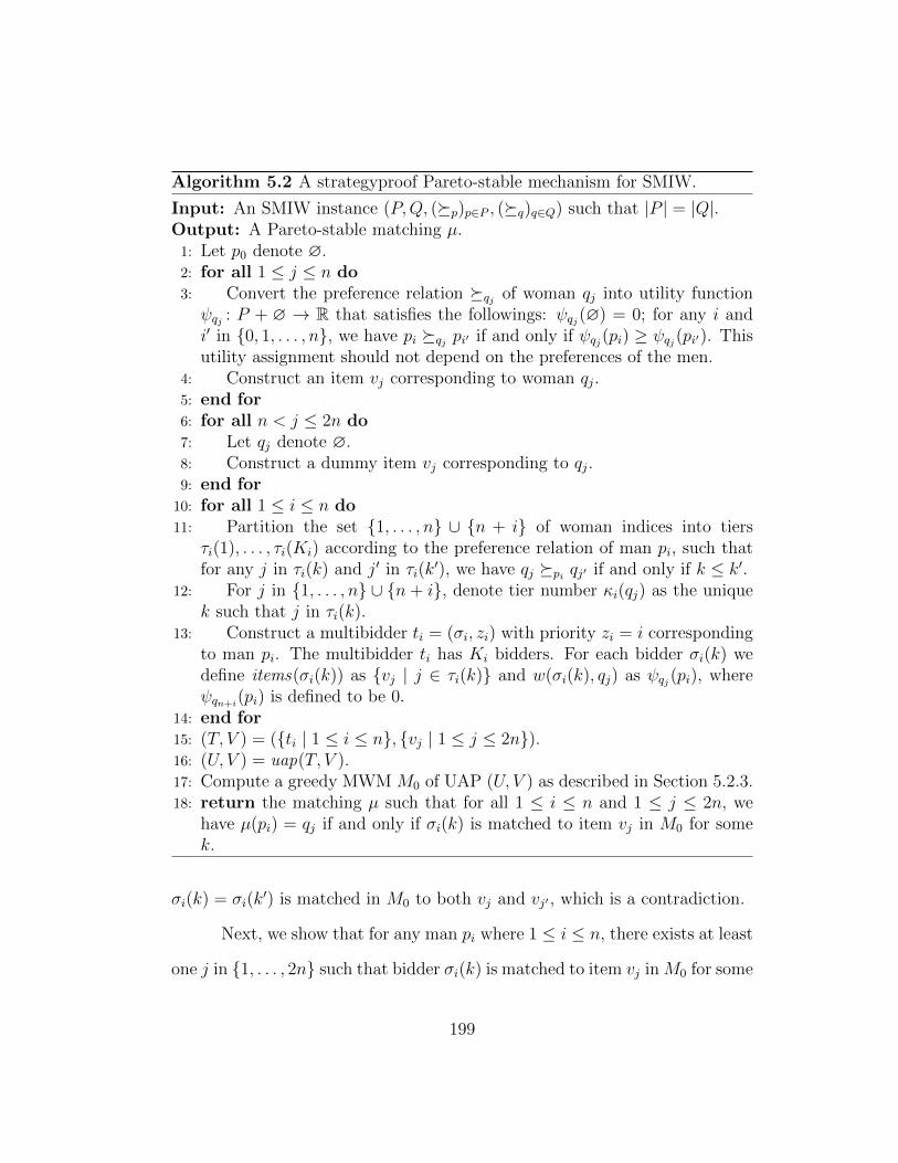
Algorithm 5.2 A strategyproof Pareto-stable mechanism for SMIW.

Input: An SMIW instance (P,Q, (p)p∈P , (q)q∈Q) such that |P | = |Q|.Output: A Pareto-stable matching µ.

1: Let p0 denote ∅.2: for all 1 ≤ j ≤ n do3: Convert the preference relation qj of woman qj into utility functionψqj : P + ∅ → R that satisfies the followings: ψqj(∅) = 0; for any i andi′ in 0, 1, . . . , n, we have pi qj pi′ if and only if ψqj(pi) ≥ ψqj(pi′). Thisutility assignment should not depend on the preferences of the men.

4: Construct an item vj corresponding to woman qj.5: end for6: for all n < j ≤ 2n do7: Let qj denote ∅.8: Construct a dummy item vj corresponding to qj.9: end for

10: for all 1 ≤ i ≤ n do11: Partition the set 1, . . . , n ∪ n + i of woman indices into tiers

τi(1), . . . , τi(Ki) according to the preference relation of man pi, such thatfor any j in τi(k) and j′ in τi(k

′), we have qj pi qj′ if and only if k ≤ k′.12: For j in 1, . . . , n ∪ n + i, denote tier number κi(qj) as the unique

k such that j in τi(k).13: Construct a multibidder ti = (σi, zi) with priority zi = i corresponding

to man pi. The multibidder ti has Ki bidders. For each bidder σi(k) wedefine items(σi(k)) as vj | j ∈ τi(k) and w(σi(k), qj) as ψqj(pi), whereψqn+i

(pi) is defined to be 0.14: end for15: (T, V ) = (ti | 1 ≤ i ≤ n, vj | 1 ≤ j ≤ 2n).16: (U, V ) = uap(T, V ).17: Compute a greedy MWM M0 of UAP (U, V ) as described in Section 5.2.3.18: return the matching µ such that for all 1 ≤ i ≤ n and 1 ≤ j ≤ 2n, we

have µ(pi) = qj if and only if σi(k) is matched to item vj in M0 for somek.

σi(k) = σi(k′) is matched in M0 to both vj and vj′ , which is a contradiction.

Next, we show that for any man pi where 1 ≤ i ≤ n, there exists at least

one j in 1, . . . , 2n such that bidder σi(k) is matched to item vj in M0 for some

199

k. For the sake of contradiction, suppose bidder σi(k) is unmatched in M0 for

all k. Let j denote n + i and let k denote κi(qj). By Lemma 5.3.5, the set U

contains bidder σi(k). Since both bidder σi(k) and item vj are unmatched by

M0, adding the pair (σi(k), vj) to M0 gives a matching of (U, V ) with the same

weight and larger cardinality. This contradicts the fact that M0 is a greedy

MWM of (U, V ).

This shows that µ(pi) is well-defined for all men pi where 1 ≤ i ≤ n.

Furthermore, since each item vj where 1 ≤ j ≤ n is matched to at most one

bidder in M0, each woman qj is matched to at most one man pi in µ where

1 ≤ i ≤ n. Hence, µ is a valid matching.

Lemma 5.4.2. Algorithm 5.2 produces an individually rational matching.

Proof. We have shown in Lemma 5.4.1 that µ is a valid matching. Consider

man pi and woman qj such that µ(pi) = qj, where i and j belong to 1, . . . , n.

Let k denote κi(qj) and let k′ denote κi(qn+i). It suffices to show that k ≤ k′

and ψqj(pi) ≥ 0.

Since µ(pi) = qj, bidder σi(k) is matched to item vj in M0. Since M0 is

an MWM, we have ψqj(pi) = w(σi(k), vj) ≥ 0.

It remains to show that k ≤ k′. For the sake of contradiction, suppose

k > k′. Since bidder σi(k) is matched to item vj in M0, by Lemma 5.3.5 the set

U contains bidder σi(k′). Since bidder σi(k

′) is not matched in M0, the dummy

item vn+i is also not matched in M0. Hence, adding the pair (σi(k′), vn+i) to

M0 gives a matching in (U, V ) with the same weight and larger cardinality.

This contradicts the fact that M0 is a greedy MWM of (U, V ).

200

Lemma 5.4.3. Algorithm 5.2 produces a weakly stable matching.

Proof. By Lemma 5.4.2, it remains only to show that µ does not admit a

strongly blocking pair. Consider man pi and woman qj′ , where i and j′ be-

long to 1, . . . , n. We want to show that (pi, qj′) does not form a strongly

blocking pair. Let qj denote µ(pi) and let pi′ denote µ(qj′), where j belongs

to 1, . . . , n ∪ n+ i and i′ belongs to 0, 1, . . . , n. It suffices to show that

either κi(qj) ≤ κi(qj′) or ψqj′ (pi′) ≥ ψqj′ (pi). For the sake of contradiction,

suppose κi(qj) > κi(qj′) and ψqj′ (pi′) < ψqj′ (pi). Let k denote κi(qj) and let k′

denote κi(qj′). Since σi(k) is matched in M0 and k′ < k, Lemma 5.3.5 implies

that the set U contains bidder σi(k′) and that σi(k

′) is unmatched in M0. We

consider two cases.

Case 1: i′ = 0. Then ψqj′ (pi) > ψqj′ (pi′) = 0. Since neither bidder

σi(k′) nor item vj′ is matched in M0, adding the pair (σi(k

′), vj′) to M0 gives

a matching of (U, V ) with a larger weight. This contradicts the fact that M0

is an MWM of (U, V ).

Case 2: i′ 6= 0. Since pi′ = µ(qj′), there exists k′′ such that bidder

σi′(k′′) is matched to vj′ in M0. Since σi(k

′) is unmatched in M0, the matching

M0 − (σi′(k′′), vj′) + (σi(k

′), vj′) is a matching of (U, V ) with weight w(M0)−

ψqj′ (pi′)+ψqj′ (pi), which is greater than w(M0). This contradicts the fact that

M0 is an MWM of (U, V ).

Lemma 5.4.4. Let µ be the matching produced by Algorithm 5.2 and let µ′

201

be a matching such that µ′(p) p µ(p) for every man p in P and

∑q∈Q

ψq(µ′(q)) ≥

∑q∈Q

ψq(µ(q)).

Then µ(p) p µ′(p) for every man p in P and

∑q∈Q

ψq(µ′(q)) =

∑q∈Q

ψq(µ(q)).

Proof. For any i such that 1 ≤ i ≤ n, let ki denote κi(µ(pi)) and let k′i denote

κi(µ′(pi)).

Below we use µ′ to construct an MWM M ′0 of (U, V ). We give the

construction of M ′0 first, and then argue that M ′

0 is an MWM of (U, V ). Let

M ′0 denote the set of bidder-item pairs (σi(k

′i), vj) such that µ′(pi) = qj where

i in 1, . . . , n and j in 1, . . . , n ∪ n + i. It is easy to see that M ′0 is a

valid matching. Notice that for any 1 ≤ i ≤ n, since µ′(pi) pi µ(pi), we have

k′i ≤ ki. So, by Lemma 5.3.5, the set U contains all bidders σi(k′i). Hence, M ′

0

is a matching of (U, V ). Furthermore, it is easy to see that

w(M ′0) =

∑1≤j≤n

ψqj(µ′(qj)) ≥

∑1≤j≤n

ψqj(µ(qj)) = w(M0).

Thus M ′0 is an MWM of (U, V ), and we have

∑1≤j≤n

ψqj(µ′(qj)) =

∑1≤j≤n

ψqj(µ(qj)).

202

Furthermore, M ′0 is an MCMWM of (U, V ) because both M ′

0 and M0 have

cardinality equal to n. Also, M ′0 is a greedy MWM of (U, V ), because both

M ′0 and M0 have priorities equal to

∑1≤i≤n zi. Hence, for each 1 ≤ i ≤ n, we

have ki ≤ k′i by Lemma 5.3.5. Thus, µ(pi) pi µ′(pi) for all 1 ≤ i ≤ n.

Lemma 5.4.5. Let µ be the matching produced by Algorithm 5.2 and µ′ be

a matching such that µ′ µ. Then, µ µ′.

Proof. Since µ′ µ, we have µ′(pi) pi µ(pi) and ψqj(µ′(qj)) ≥ ψqj(µ(qj)) for

every i and j in 1, . . . , n. So, by Lemma 5.4.4, we have µ(pi) pi µ′(pi) for

every i in 1, . . . , n and

∑1≤j≤n

ψqj(µ′(qj)) =

∑1≤j≤n

ψqj(µ(qj)).

Therefore, ψqj(µ′(qj)) = ψqj(µ(qj)) for every j in 1, . . . , n. This shows that

µ µ′.

Lemma 5.4.6. Consider Algorithm 5.2. Suppose µ(pi) = qj, where 1 ≤ i ≤ n

and j belongs to 1, . . . , n ∪ n+ i. Then, we have

(ψqj(pi), i) ≥ threshold((T − ti, V ), vj). (5.3)

Furthermore, for all j′ in 1, . . . , n ∪ n + i such that κi(qj′) < κi(qj), we

have

(ψqj′ (pi), i) < threshold((T − ti, V ), vj′). (5.4)

Proof. Let k denote κi(qj). Since µ(pi) = qj, we know that bidder σi(k)

203

is matched to item vj in M0. So, inequality (5.1) of Lemma 5.3.8 implies

inequality (5.3), because w(σi(k), vj) = ψqj(pi) and zi = i.

Now, suppose κi(qj′) < κi(qj). Let k′ denote κi(qj′). Since k′ < k, in-

equality (5.2) of Lemma 5.3.8 implies inequality (5.4), because w(σi(k′), vj′) =

ψqj′ (pi) and zi = i.

Theorem 5.4.7. Algorithm 5.2 is a strategyproof Pareto-stable mechanism

for the stable marriage problem with incomplete and weak preferences (for any

fixed choice of utility assignment).

Proof. We have shown in Lemma 5.4.3 that the algorithm produces a weakly

stable matching. Moreover, Lemma 5.4.5 shows that the weakly stable match-

ing produced is not Pareto-dominated by any other matching. Hence, the

algorithm produces a Pareto-stable matching. It remains to show that the

algorithm is a strategyproof mechanism.

Suppose man pi expresses ′pi instead of his true preference relation

pi , where 1 ≤ i ≤ n. Let µ and µ′ be the resulting matchings given pi and

′pi , respectively. Let qj denote µ(pi) and let qj′ denote µ′(pi), where j and j′

belong to 1, . . . , n ∪ n + i. Let k denote κi(qj) and let k′ denote κi(qj′),

where κi(·) denotes the tier number with respect to pi . It suffices to show

that k ≤ k′. For the sake of contradiction, suppose k > k′.

Let (T, V ) be the IUAP, let ti be the multibidder corresponding to man

pi, and let vj′ be the item corresponding to woman qj′ constructed in the algo-

rithm given input pi . Since µ(pi) = qj, by inequality (5.4) of Lemma 5.4.6,

204

we have

(ψqj′ (pi), i) < threshold((T − ti, V ), vj′).

Now, consider the behavior of the algorithm when preference relation

pi is replaced with ′pi . Let (T ′, V ′) be the IUAP, let t′i be the multibidder

corresponding to man pi, and let v′j′ be the item corresponding to woman qj′

constructed in the algorithm given input ′pi . Since µ′(pi) = qj′ , by inequal-

ity (5.3) of Lemma 5.4.6, we have

(ψqj′ (pi), i) ≥ threshold((T ′ − t′i, V ′), v′j′).

Notice that in Algorithm 5.2, the only part of the IUAP instance that

depends on the preferences of man pi is the multibidder corresponding to man

pi. In particular, we have T − ti = T ′ − t′i, V = V ′, and vj′ = v′j′ . Hence, we

get

(ψqj′ (pi), i) < threshold((T − ti, V ), vj′)

= threshold((T ′ − t′i, V ′), v′j′)

≤ (ψqj′ (pi), i),

which is a contradiction.

205

5.5 College Admissions with Indifferences

Our strategyproof mechanism can be generalized to the college admissions

model with weak preferences. In this model, students and colleges play the

roles of men and women, respectively, and colleges are allowed to be matched

with multiple students up to their capacities. We can apply our mechanism

for SMIW by transforming each student to a man and each slot of a college to

a woman in a standard fashion.

The college admissions model with weak preferences (CAW) involves a

set P of students and a set Q of colleges. The preference relation of each

student p in P is specified as a binary relation p over Q + ∅ that satisfies

transitivity and totality, where ∅ denotes being unmatched. The preference

relation of each college q in Q over individual students is specified as a binary

relation q over P +∅ that satisfies transitivity and totality, where ∅ denotes

being unmatched. Each college q in Q has an associated integer capacity

cq > 0. We will use p and q to denote the asymmetric parts of p and q,

respectively.

The colleges’ preference relations over individual students can be ex-

tended to group preference relations using responsiveness [49]. We say that a

transitive and reflexive relation ′q over the power set 2P is responsive to the

preference relation q if the following conditions hold: for any S ⊆ P and p

in P \ S, we have p q ∅ if and only if S + p ′q S; for any S ⊆ P and any p

and p′ in P \ S, we have p q p′ if and only if S + p ′q S + p. Furthermore,

we say that a relation ′q is minimally responsive to the preference relation q

206

if it is responsive to the preference relation q and does not strictly contain

another relation that is responsive to the preference relation q.

A (capacitated) matching is a function µ from P to Q+∅ such that for

any college q in Q, there exists at most cq students p in P for which µ(p) = q.

Given a matching µ and a college q in Q, we let µ(q) denote p ∈ P | µ(p) = q.

A matching µ is individually rational if for any student p in P and

college q in Q such that µ(p) = q, we have q p ∅ and p q ∅. A pair

(p′, q) in P × Q is said to form a strongly blocking pair for a matching µ if

q p′ µ(p′) and at least one of the following two conditions holds: (1) there

exists a student p in P such that µ(p) = q and p′ q p; (2) |µ(q)| < cq and

p′ q ∅. A matching is weakly stable if it is individually rational and does not

admit a strongly blocking pair.

Let ′q be the group preference associated with college q in Q. For any

matching µ and µ′, we say that the binary relation µ µ′ holds if for every

student p in P and college q in Q, we have µ(p) p µ′(p) and µ(q) ′q µ′(q).

We let denote the asymmetric part of . We say that a matching µ Pareto-

dominates another matching µ′ if µ µ′. We say that a matching is Pareto-

optimal if it is not Pareto-dominated by any other matching. A matching is

Pareto-stable if it is Pareto-optimal and weakly stable.

A mechanism is an algorithm that, given (P,Q, (p)p∈P , (q)q∈Q, (cq)q∈Q),

produces a matching µ. A mechanism is said to be strategyproof (for the stu-

dents) if for any student p in P expressing preference ′p instead of their true

preference p, we have µ(p) p µ′(p), where µ and µ′ are the matchings pro-

207

duced by the mechanism given p and ′p, respectively, when all other inputs

are fixed.

Without loss of generality, we may assume that the number of stu-

dents equals the total capacity of the colleges. So, P = pi1≤i≤|P | and

Q = qj1≤j≤|Q| such that |P | =∑

1≤j≤|Q| cqj .

5.5.1 Algorithm 5.3

The computation of a matching for CAW is shown in Algorithm 5.3. We

transform each student to a man in line 1, and each slot of a college to a

woman in line 2. This forms an SMIW. Using this SMIW, we produce a

matching by invoking Algorithm 5.2 in lines 8 and 9.

The following results are analogues of that in Section 5.4.1

Lemma 5.5.1. Algorithm 5.3 produces an individually rational matching.

Proof. It is easy to see that µ satisfies the capacity constraints because each

college qj is associated with cqj women q′jk and each woman can be matched

with at most one man in µ0 by Lemma 5.4.1.

The individual rationality of µ follows from the individual rationality

of µ0. Let pi in P and qj in Q such that µ(pi) = qj. Then µ0(p′i) = q′jk for

some k. By Lemma 5.4.2, we have q′jk p′i ∅ and p′i q′jk ∅. Hence, qj pi ∅

and pi qj ∅.

Lemma 5.5.2. Algorithm 5.3 produces a weakly stable matching.

208

Algorithm 5.3 A strategyproof Pareto-stable mechanism for CAW.

Input: An CAW instance (P,Q, (p)p∈P , (q)q∈Q, (cq)q∈Q) such that |P | =∑q∈Q cq.

Output: A Pareto-stable matching µ.1: For each 1 ≤ i ≤ |P |, construct man p′i corresponding to student pi.2: For each 1 ≤ j ≤ |Q|, construct women q′j1, . . . , q

′jc corresponding to college

qj with capacity c = cqj .3: (P ′, Q′) = (p′i | 1 ≤ i ≤ |P |, q′jk | 1 ≤ j ≤ |Q| and 1 ≤ k ≤ cqj).4: Let p0 denote ∅. Let p′0 denote ∅.5: Let q0 denote ∅. Let q′00 denote ∅.6: For each 1 ≤ i ≤ |P |, define the preference relation p′i over Q′ + q′00 for

man p′i using the preference relation of his corresponding student, suchthat q′jk p′i q

′j′k′ if and only if qj pi qj′ .

7: For each 1 ≤ j ≤ |Q| and 1 ≤ k ≤ cqj , define the preference relation q′jkover P ′+p′0 for woman q′jk using the preference relation of her correspond-ing college, such that p′i q′jk p

′i′ if and only if pi qj pi′ .

8: Compute matching µ0 for SMIW (P ′, Q′, (p′)p′∈P ′ , (q′)q′∈Q′) using Algo-rithm 5.2, where we require the utility functions associated with the samecollege to be the same.

9: return the matching µ, such that for all 1 ≤ i ≤ |P | and 0 ≤ j ≤ |Q|, wehave µ(pi) = qj if and only if µ0(p

′i) = q′jk for some k.

Proof. By Lemma 5.5.1, it remains only to show that µ does not admit a

strongly blocking pair. Consider student pi′ in P and college qj in Q. In what

follows, we use the weak stability of µ0 to show that (pi′ , qj) does not form a

strongly blocking pair.

Let q′j′k′ denote µ0(p′i′). It is possible that q′j′k′ = ∅, in which case

j′ = k′ = 0. For 1 ≤ k ≤ cqj , let p′ik denote µ0(q′jk), where p′ik belongs

to P ′ + p′0. By Lemma 5.4.3, for any 1 ≤ k ≤ cqj , either q′j′k′ p′i′ q′jk or

p′ik q′jk p′i′ , for otherwise (p′i′ , q

′jk) forms a strongly blocking pair.

Suppose q′j′k′ p′i′ q′jk for some 1 ≤ k ≤ cqj . Then qj′ pi′ qj, and hence

209

(pi′ , qj) does not form a strongly blocking pair.

Otherwise, p′ik q′jk p′i′ for all 1 ≤ k ≤ cqj . Then pik qj pi′ for all

1 ≤ k ≤ cqj . In particular, we have pik qj pi′ for all students pik in P

such that µ(pik) = qj. Furthermore, if |µ(qj)| < cqj , then pik = ∅ for some

1 ≤ k ≤ cqj . Hence ∅ qj pi′ . It follows that (pi′ , qj) does not form a strongly

blocking pair.

Lemma 5.5.3. Suppose that for every college q in Q, the group preference

relation ′q is minimally responsive to q. Let µ be the matching produced

by Algorithm 5.3 and let µ′ be a matching such that µ′ µ. Then µ µ′.

Proof. Since µ′ is a matching that satisfies the capacity constraints, we can

construct an SMIW matching µ′0 : P ′ → Q′ + q′00 such that for all 1 ≤ i ≤ |P |

and 0 ≤ j ≤ |Q|, we have µ′(pi) = qj if and only if µ0(p′i) = q′jk for some k.

Since µ′ µ, we have µ′(pi) pi µ(pi) for every 1 ≤ i ≤ |P | and

µ′(qj) ′qj µ(qj) for every 1 ≤ j ≤ |Q|. Thus µ′0(p′i) p′i µ0(p

′i) for every

1 ≤ i ≤ |P | and

∑1≤k≤cqj

ψq′jk(µ′0(q′jk)) ≥

∑1≤k≤cqj

ψq′jk(µ0(q′jk))

for every 1 ≤ j ≤ |Q|. Hence, by Lemma 5.4.4, we have µ0(p′i) p′i µ

′0(p′i) for

every 1 ≤ i ≤ |P | and

∑1≤j≤|Q|

∑1≤k≤cqj

ψq′jk(µ′0(q′jk)) =

∑1≤j≤|Q|

∑1≤k≤cqj

ψq′jk(µ0(q′jk)).

210

Therefore, we have µ(pi) pi µ′(pi) for every 1 ≤ i ≤ |P | and

∑1≤k≤cqj

ψq′jk(µ′0(q′jk)) =

∑1≤k≤cqj

ψq′jk(µ0(q′jk))

for every 1 ≤ j ≤ |Q|. We conclude that µ(qj) ′qj µ′(qj) for every 1 ≤ j ≤ |Q|.

Thus µ µ′.

Theorem 5.5.4. Suppose that for every college q in Q, the group preference

relation ′q is minimally responsive to q. Algorithm 5.3 is a strategyproof

Pareto-stable mechanism for the college admissions problem with weak pref-

erences (for any fixed choice of utility assignment).

Proof. We have shown in Lemma 5.5.2 that Algorithm 5.3 produces a weakly

stable matching. Moreover, Lemma 5.5.3 shows that the weakly stable match-

ing produced is not Pareto-dominated by any other matching. Hence, Algo-

rithm 5.3 produces a Pareto-stable matching.

To show that Algorithm 5.3 provides a strategyproof mechanism, sup-

pose student pi expresses ′pi instead of their true preference relation pi ,

where 1 ≤ i ≤ |P |. Let µ and µ′ be the matchings produced by Algorithm 5.3

given pi and ′pi , respectively. Let µ0 and µ′0 be the SMIW matching pro-

duced by the call to Algorithm 5.2 (line 8 of Algorithm 5.3) given pi and ′pi ,

respectively.

Notice that in Algorithm 5.3, the only part of the stable marriage in-

stance that depends on the preferences of student pi is the preference rela-

tion corresponding to man p′i. Since Algorithm 5.2 is strategyproof by The-

211

orem 5.4.7, we have µ0(p′i) p′i µ

′0(p′i) where p′i is the preference relation of

man p′i in the algorithm given pi . Hence, µ(pi) pi µ′(pi).

Our algorithm admits an O(n4)-time implementation, where n is the

sum of the number of students and the total capacities of all the colleges,

because the reduction from CAW to IUAP takes O(n2) time, and lines 16

and 17 of Algorithm 5.2 can be implemented in O(n4) time using the version

of the incremental Hungarian method discussed in Sections 5.2.3 and 5.3.2.

5.5.2 Further Discussion

In our SMIW and CAW algorithms, we transform the preference relations of

the women and colleges into real-valued utility functions. One way to do this

is to take

ψq(p) = |p′ ∈ P + ∅ : p q p′| − |p′ ∈ P + ∅ : ∅ q p′|.

This is by no means the only way. In fact, different ways of assigning the

utilities can affect the outcome. Nonetheless, our mechanisms remain strate-

gyproof for the men as long as the utility assignment is fixed and independent

of the preferences of the men, as shown in Theorems 5.4.7 and 5.5.4.

We can also consider the scenario where each college expresses their

preferences directly in terms of a utility function instead of a preference re-

lation. Such utility functions provide another way to extend preferences over

individuals to group preferences. If a college q expresses the utility function ψq

212

over individual students in P + ∅, we can define the group preference induced

by additive utility ψq as a binary relation ′q over 2P such that S ′q S ′ if and

only if ∑p∈S

ψq(p) ≥∑p∈S′

ψq(p).

Our algorithm can accept such utility functions as input in lieu of constructing

them by some utility assignment method. It is not hard to see that the mech-

anism remains Pareto-stable and strategyproof when the group preferences of

the colleges are induced by additive utilities.

213

Chapter 6

Establishing Group

Strategyproofness

In this chapter, we establish that the strategyproof (for the men) and Pareto-

stable mechanism of Chapter 5 is also group strategyproof (for the men). We

do so by showing that the mechanism of Chapter 5 coincides with the group

strategyproof Pareto-stable mechanism (for the same model) introduced by

Domanic et al. [17]. 1

In Section 6.1, we briefly describe the mechanism of [17], and we state

the theorem summarizing the group strategyproofness result of [17] and a

lemma that is used in Section 6.3; the details and the proofs are available

1We wish to clarify the relationship between the results presented in this chapter and [17].There are two main results established in [17]: a group strategyproof Pareto-stable mecha-nism for SMIW; the equivalence of that mechanism and the mechanism of this dissertation(Chapter 5). The first result is expected to be included in the dissertation work of coauthorChi-Kit Lam. The second result is part of this dissertation. In order to present the secondresult, we will need to review some definitions, a theorem, and a lemma associated with thefirst result.

214

in [17]. Then, in Section 6.2, we restate the strategyproof SMIW mechanism

of Chapter 5 (Algorithm 5.2) using the notation of [17]. Finally, in Section 6.3,

we show that the mechanism of Chapter 5, which is restated in Section 6.2,

coincides with the group strategyproof Pareto-stable mechanism of [17], and

hence is group strategyproof (Theorem 6.3.17).

6.1 A Group Strategyproof Pareto-Stable Mech-

anism

The assignment game of Shapley and Shubik [55] involves a two-sided matching

market with monetary transfers where the agents have unit-slope linear utility

functions. This model has been generalized to allow agents to have continu-

ous, invertible, and increasing utility functions [12, 14, 46]. Some models that

generalize both the assignment game and the stable marriage have also been

developed, but those models are not concerned with the strategic behavior of

agents [27, 60]. The mechanism of [17] casts the stable marriage problem as an

appropriate market in the model of Demange and Gale [14]. In Section 6.1.1,

we review key concepts in the work of Demange and Gale, and introduce the

tiered-slope market as a special form of the generalized assignment game in

which the slopes of the utility functions are powers of a large fixed number.

Then, in Section 6.1.2, we formally define group strategyproofness for the sta-

ble marriage model with indifferences. Finally, in Section 6.1.3, we describe

our approach for converting a stable marriage market with indifferences into

215

an associated tiered-slope market. Theorem 6.1.1 shows that group strate-

gyproofness for the men in the stable marriage market with indifferences is

achieved by man-optimality in the associated tiered-slope market.

6.1.1 Tiered-Slope Markets

The generalized assignment game studied by Demange and Gale [14] involves

two disjoint sets I and J of agents, which we call the men and the women,

respectively. We assume that the sets I and J do not contain the element ∅,

which we use to denote being unmatched. For each man i in I and woman j in

J , the compensation function fi,j(ui) represents the compensation that i needs

to receive in order to attain utility ui when he is matched to j. Similarly, for

each man i and woman j, the compensation function gi,j(vj) represents the

compensation that j needs to receive in order to attain utility vj when she is

matched to i. Moreover, each man i has a reserve utility ri and each woman

j has a reserve utility sj.

Throughout this chapter, we assume that the compensation functions

are of the form

fi,j(ui) = uiλ−ai,j and gi,j(vj) = vj − (bi,jN + πi)

and the reserve utilities are of the form

ri = πiλai,∅ and sj = b∅,jN,

216

such that the following conditions hold: π ∈ ZI ; N ∈ Z; λ ∈ Z; a ∈ ZI×(J+∅);

b ∈ Z(I+∅)×J ;

N > maxi∈I

πi ≥ mini∈I

πi ≥ 1;

λ ≥ max(i,j)∈(I+∅)×J

(bi,j + 1)N ≥ min(i,j)∈(I+∅)×J

(bi,j + 1)N ≥ N.

We refer to this market as the tiered-slope market M = (I, J, π,N, λ, a, b). For

better readability, we write expλ(ξ) to denote λξ.

Let M be a tiered-slope market (I, J, π,N, λ, a, b). A matching µ is a

function from I to J + ∅ such that for any woman j in J , we have µ(i) = j

for at most one man i. Given a matching µ and a woman j in J , we denote

µ(j) =

i if µ(i) = j

0 if there is no man i in I such that µ(i) = j.

A utility vector of the men I is a vector u in RI . A utility vector of the women

J is a vector v in RJ . An outcome is a triple (µ, u, v), where µ is a matching,

u is a utility vector of the men I, and v is a utility vector of the women J .

An outcome (µ, u, v) is feasible if the following conditions hold for each man i

and woman j: if µ(i) = j, then fi,j(ui) +gi,j(vj) ≤ 0; if µ(i) = ∅, then ui = ri;

if µ(j) = ∅, then vj = sj. A feasible outcome (µ, u, v) is individually rational

if ui ≥ ri and vj ≥ sj for each man i and woman j. An individually rational

outcome (µ, u, v) is stable if fi,j(ui) + gi,j(vj) ≥ 0 for each man i and woman

j.

A stable outcome (µ, u, v) is man-optimal if for any stable outcome

217

(µ′, u′, v′) we have ui ≥ u′i for every man i ∈ I. It has been shown that

man-optimal outcomes always exist [14, Property 2].

6.1.2 Stable Marriage and Group Strategyproofness

When we formally introduced the SMIW model in Section 5.4, we used P

and Q to denote the sets of men and women, respectively, and we used pi

and qj to denote an individual man and a woman, respectively, where i and j

were used to denote the indices of men and woman. In the remainder of this

chapter, we adopt the notation of [17] and use I, J , i, and j to denote a set

of men, a set of women, an individual man, and a woman, respectively. All

the definitions of Section 5.4 carry over here with the revised notation. For

the sake of completeness, we enumerate here the other resulting notational

changes: the binary relation over J + ∅ specifying the preference relation

of a man i is denoted by i; the binary relation over I + ∅ specifying the

preference relation of a woman j is denoted by j; an SMIW instance is a tuple

(I, J, (i)i∈I , (j)j∈J), which we call a stable marriage market ; a mechanism

is an algorithm that, given a stable marriage market (I, J, (i)i∈I , (j)j∈J),

produces a matching µ. In the remainder of this chapter, we do not need

the dummy men or women that we introduced in Section 5.4 for convenience.

Thus we relax the assumption that |I| = |J | in a stable marriage market

(I, J, (i)i∈I , (j)j∈J).

We now formally define group strategyproofness. A mechanism is said

to be group strategyproof (for the men) if for any two different preference

218

profiles (i)i∈I and (′i)i∈I , there exists a man i0 ∈ I with preference rela-

tion i0 different from ′i0 such that µ(i0) i0 µ′(i0), where µ and µ′ are

the matchings produced by the mechanism given (I, J, (i)i∈I , (j)j∈J) and

(I, J, (′i)i∈I , (j)j∈J), respectively. (Such a man i0 belongs to the coalition,

but is not matched to a strictly preferred woman by expressing preference

relation ′i0 instead of his true preference relation i0 .)

6.1.3 An Associated Tiered-Slope Market and A Mech-

anism

The group strategyproof Pareto-stable mechanism of [17] for SMIW first cre-

ates a tiered-slope market assoicated with the given stable marriage market, in

a manner we describe shortly, and then returns a matching corresponding to

a man-optimal outcome of this tiered-slope market. The result is summarized

in Theorem 6.1.1 below; the proof can be found in [17]. In the remainder of

this section, we describe how to create a tiered-slope market assoicated with

a stable marriage market, and we present a lemma to be used in Section 6.3

to provide a lower bound on the utilities of men in the man-optimal outcomes

of certain markets.

We construct a tiered-slope market M = (I, J, π,N, λ, a, b) associated

with a stable marriage market (I, J, (i)i∈I , (j)j∈J) as follows. We take N at

least |I|+ 1, and for each man i in I, we associate with i a fixed and distinct

priority πi from the set 1, 2, . . . , |I|. We convert the preference relations (i

)i∈I of the men to integer-valued (non-transferable) utilities a ∈ ZI×(J+∅) such

219

that for each man i in I and two elements j1 and j2 in J+∅, we have j1 i j2 if

and only if ai,j1 ≥ ai,j2 . Similarly, we convert the preference relations (j)j∈J

of the women to integer-valued (non-transferable) utilities b ∈ Z(I+∅)×J such

that for each woman j in J and two elements i1 and i2 in I + ∅, we have

i1 j i2 if and only if bi1,j ≥ bi2,j ≥ 1. Finally, we take

λ = maxi∈I+∅j∈J

(bi,j + 1)N.

In order to achieve group strategyproofness, we require the parameter

N and the priorities π of the men to be independent of the preferences (i)i∈I

of the men. We further require that b does not depend on the preferences

(i)i∈I of the men, and that ai0,j0 does not depend on the other preferences

(i)i∈I\i0 for any man i0 ∈ I and woman j0 ∈ J + ∅. In other words, each

man i0 is only able to manipulate his own utilities (ai0,j)j∈J+∅. One way to

satisfy these conditions is as follows: for each man i0 in I and each element j0

in J + ∅, set ai0,j0 to the number of elements j in J + ∅ such that j0 i0 j;

for each woman j0 in J and each element i0 in I + ∅, set bi0,j0 to the number

of elements i in I + ∅ such that i0 j0 i.

Theorem 6.1.1. If a mechanism produces matchings that correspond to man-

optimal outcomes of the tiered-slope markets associated with the stable mar-

riage markets, then it is group strategyproof and Pareto-stable.

The following lemma is used to establish Lemma 6.3.8 in Section 6.3,

which provides a lower bound on the utilities of men in the man-optimal out-

220

comes of certain markets; its proof can be found in [17].

Lemma 6.1.2. LetM = (I, J, π,N, λ, a, b) be the tiered-slope market associ-

ated with stable marriage market (I, J, (i)i∈I , (j)j∈J), and let r denote the

reserve utility vector of the men in M. Let r′ be a reserve utility vector of

the men such that the following conditions hold: (i) r′ ≥ r; (ii) for any man

i and any integer k, either r′i expλ(k) is an integer or 0 < r′i expλ(k) < 1. Let

M′ be the market that is equal to M except that the reserve utilities of the

men are given by r′, and let (µ, u, v) be a man-optimal outcome inM′. Then

expλ(ai,µ(i)) ≤ ui for every man i ∈ I.

6.2 Algorithm 5.2 Revisited

In this section, in order to suit the presentation of the current chapter, we

present the strategyproof SMIW mechanism of Chapter 5 (Algorithm 5.2)

using the notation of Section 6.1; the mechanism with the new notation is

given in Algorithm 6.1. For each woman j, we construct an item, denoted

item(j), in line 3. For each man i, we construct a dummy item, denoted

item∅(i), in line 7, and a multibidder, denoted multibidder(i), in line 8, by

examining the tiers of preference of the men and the utilities of the women.

The set zi | i ∈ I of priorities of the multibidders is equal to 1, . . . , |I|, and

we assume that the men have no control over the assignment of the priorities.

These multibidders and items form an IUAP, from which we obtain a UAP and

a greedy MWM M . Finally, in line 13, we use M to determine the match of

221

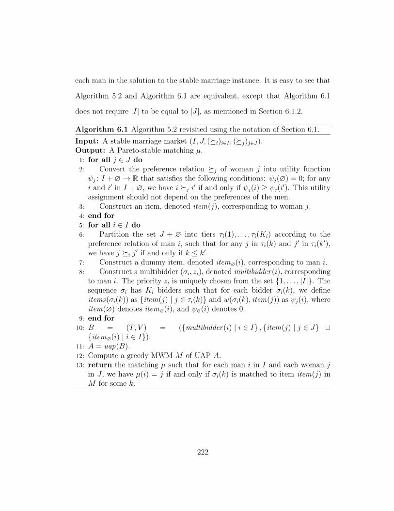
each man in the solution to the stable marriage instance. It is easy to see that

Algorithm 5.2 and Algorithm 6.1 are equivalent, except that Algorithm 6.1

does not require |I| to be equal to |J |, as mentioned in Section 6.1.2.

Algorithm 6.1 Algorithm 5.2 revisited using the notation of Section 6.1.

Input: A stable marriage market (I, J, (i)i∈I , (j)j∈J).Output: A Pareto-stable matching µ.

1: for all j ∈ J do2: Convert the preference relation j of woman j into utility functionψj : I + ∅→ R that satisfies the following conditions: ψj(∅) = 0; for anyi and i′ in I + ∅, we have i j i′ if and only if ψj(i) ≥ ψj(i

′). This utilityassignment should not depend on the preferences of the men.

3: Construct an item, denoted item(j), corresponding to woman j.4: end for5: for all i ∈ I do6: Partition the set J + ∅ into tiers τi(1), . . . , τi(Ki) according to the

preference relation of man i, such that for any j in τi(k) and j′ in τi(k′),

we have j i j′ if and only if k ≤ k′.7: Construct a dummy item, denoted item∅(i), corresponding to man i.8: Construct a multibidder (σi, zi), denoted multibidder(i), corresponding

to man i. The priority zi is uniquely chosen from the set 1, . . . , |I|. Thesequence σi has Ki bidders such that for each bidder σi(k), we defineitems(σi(k)) as item(j) | j ∈ τi(k) and w(σi(k), item(j)) as ψj(i), whereitem(∅) denotes item∅(i), and ψ∅(i) denotes 0.

9: end for10: B = (T, V ) = (multibidder(i) | i ∈ I , item(j) | j ∈ J ∪item∅(i) | i ∈ I).

11: A = uap(B).12: Compute a greedy MWM M of UAP A.13: return the matching µ such that for each man i in I and each woman j

in J , we have µ(i) = j if and only if σi(k) is matched to item item(j) inM for some k.

222

6.3 Equivalence of the Two Mechanisms

In this section, we fix a stable marriage market (I, J, (i)i∈I , (j)j∈J) and

an associated tiered-slope market M = (I, J, π,N, λ, a, b). As in Section 6.1,

fi,j(ui) denotes the compensation that man i needs to receive in order to

attain utility ui in M when he is matched to woman j, and gi,j(vj) denotes

the compensation that woman j needs to receive in order to attain utility vj in

M when she is matched to man i. We let r denote the reserve utility vector of

the men in M, and we let s denote the reserve utility vector of the women in

M. We consider an execution of Algorithm 6.1 on the stable marriage market

(I, J, (i)i∈I , (j)j∈J), and we let B = (T, V ) denote the IUAP constructed at

line 10 of this execution. We assume that B is constructed in such a way that

the following conditions hold: for each man i, the priority of multibidder(i)

is πi; the offers of the multibidders in B, i.e., the weights of the edges of B,

satisfy the conditions stated in the last paragraph of Section 6.3.1 below. With

the assumption that these conditions hold, we show in Theorem 6.3.16 that

the set of greedy MWMs of uap(B) corresponds to the set of man-optimal

matchings of M.

Algorithm 6.1 computes a greedy MWM of the UAP uap(B) in lines 11

and 12. Recall that we defined uap(B) in Section 5.3.1 by giving an algorithm

that converts an IUAP to a UAP, namely Algorithm 5.1. In this section, we

analyze the executions of Algorithm 5.1 with input B in order to relate the

greedy MWMs of uap(B) that Algorithm 6.1 computes to the man-optimal

matchings of M. As outlined in Section 1.2.3, our approach is based on the

223

technique of analyzing market instances in which the agents and their utility

functions are fixed, while the reserve utilities vary. As noted by Roth and So-

tomayor [51, Chapter 9], lowering the reserve utility of an agent is analogous to

extending the preferences of an agent in the stable marriage model, a technique

used to study structural properties of the stable marriage model. Building on

this idea, for each iteration of Algorithm 5.1, we inductively show a bijection

(Lemmas 6.3.11 and 6.3.14) from the set of greedy MWMs of the UAP main-

tained at that iteration to the man-optimal matchings of the corresponding

tiered-slope market, where the reserve utilities are adjusted to “reveal” only

the preferences that are present in the UAP.

In the preceding sections, the terms “feasible”, “individually rational”,

“stable”, and “man-optimal” are used only for outcomes. Throughout this

section, however, we also use these terms for payoffs and matchings, as in [14].

Here we briefly review the related definitions. A pair (u, v) consisting of a

utility vector u of the men and a utility vector v of the women is a payoff. For

any feasible outcome (µ, u, v) of a market M′, we say that (u, v) is a feasible

payoff of M′, and that µ is compatible with (u, v). A feasible payoff (u, v) is

individually rational if ui ≥ ri for each man i and vj ≥ sj for each woman j.

If an outcome (µ, u, v) is stable (resp., man-optimal) for a market M′, then

we say that µ is a stable (resp., man-optimal) matching ofM′, and that (u, v)

is a stable (resp., man-optimal) payoff in M′. For a given market, there is

a unique man-optimal payoff, but there can be more than one man-optimal

matching.

224

6.3.1 Edge Weights of the IUAP

We start our discussion by introducing some useful mappings from items to

women and from man-woman pairs to bidders. Recall that, for each woman

j, item(j) is constructed at line 3 of Algorithm 6.1, and for each man i,

item∅(i) is constructed at line 7 and multibidder(i) is constructed at line 8.

For any non-dummy item v in V , we define woman(v) as the woman in J

associated with v. (Thus for each woman j, woman(item(j)) is equal to j.)

For any dummy item v in V , we define woman(v) as ∅. (Thus for each

man i, woman(item∅(i)) is equal to ∅.) For any subset V ′ of V , we define

women(V ′) as woman(v) | v ∈ V ′. For any man i in I and any element

j in J + ∅, we define bidder(i, j) as the bidder in multibidder(i) such that

women(items(bidder(i, j))) contains j. Remark: For each man i, the dummy

item item∅(i) belongs to items(bidder(i,∅)).

In the remainder of the paper, for any man i and any woman j, we use

the shorthand w(i, j) to denote w(bidder(i, j), item(j)), and w(i,∅) to denote

w(bidder(i,∅), item∅(i)).

For any matching µ ofM, we define b(µ) as∑

µ(j)6=∅ bµ(j),j+∑

µ(j)=∅ b∅,j,

and we define w(µ) as∑

µ(j)6=∅ w(µ(j), j).

We assume that the IUAP B is constructed so that the w(i, j)’s satisfy

the following conditions: (i) for any man i, w(i,∅) = 0; (ii) for any two

matchings µ and µ′ of M, w(µ) ≥ w(µ′) if and only if b(µ) ≥ b(µ′). It is easy

to see that one way to satisfy these conditions is to set ψj(i) = bi,j − b∅,j in

Algorithm 6.1.

225

6.3.2 Tiered-Slope Market Matchings and Greedy MWMs

In this section, we first introduce certain mappings from the tiered-slope mar-

ket matchings to the UAP matchings, and we define weights for these tiered-

slope market matchings. Then, in Lemma 6.3.6, we show that these mappings

define bijections from certain sets of tiered-slope market matchings — those

maximizing the weights we introduce — to the sets of greedy MWMs. We

start with some useful definitions.

For any configuration C = (A,B) and any man i, we define the predi-

cate Pall(C, i) to hold if i has revealed all of his acceptable tiers in C, i.e., if

bidder(i,∅) belongs to A.

Lemma 6.3.1. Let C = (A,B) be a configuration and let i be a man such that

Pall(C, i) holds. Then for each greedy MWM M of A, some bidder associated

with i is matched in M .

Proof. Suppose the claim does not hold, and let M be a greedy MWM of A

such that there is no bidder associated with i that is matched inM . Then, since

bidder(i,∅) and item∅(i) belong toA, w(i,∅) = 0, and priority(bidder(i,∅)) >

0, we deduce that the matching M ′ = M+(bidder(i,∅), item∅(i)) is an MWM

of A such that priority(M ′) > priority(M), a contradiction.

We define C1 as the configuration (A,B) where A is the UAP that

reveals only the first bidder of each multibidder in T . We say that an exe-

cution of Algorithm 5.1 invoked with input B is canonical if C1 is equal to

the configuration that the program variable C stores at some iteration of this

226

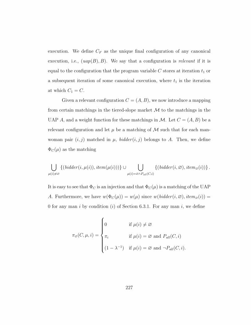
execution. We define CF as the unique final configuration of any canonical

execution, i.e., (uap(B), B). We say that a configuration is relevant if it is

equal to the configuration that the program variable C stores at iteration t1 or

a subsequent iteration of some canonical execution, where t1 is the iteration

at which C1 = C.

Given a relevant configuration C = (A,B), we now introduce a mapping

from certain matchings in the tiered-slope market M to the matchings in the

UAP A, and a weight function for these matchings inM. Let C = (A,B) be a

relevant configuration and let µ be a matching of M such that for each man-

woman pair (i, j) matched in µ, bidder(i, j) belongs to A. Then, we define

ΦC(µ) as the matching

⋃µ(i)6=∅

(bidder(i, µ(i)), item(µ(i))) ∪⋃

µ(i)=∅∧Pall (C,i)

(bidder(i,∅), item∅(i)) .

It is easy to see that ΦC is an injection and that ΦC(µ) is a matching of the UAP

A. Furthermore, we have w(ΦC(µ)) = w(µ) since w(bidder(i,∅), item∅(i)) =

0 for any man i by condition (i) of Section 6.3.1. For any man i, we define

π∅(C, µ, i) =

0 if µ(i) 6= ∅

πi if µ(i) = ∅ and Pall(C, i)

(1− λ−1) if µ(i) = ∅ and ¬Pall(C, i).

227

We define π∅(C, µ) as∑

i∈I π∅(C, µ, i). Remark: It is easy to see that

π∅(C, µ) =∑µ(i)=∅

π∅(C, µ, i) =∑

µ(i)=∅∧Pall (C,i)

πi +∑

µ(i)=∅∧¬Pall (C,i)

(1− λ−1).

Finally, we define WC(µ) as

N · b(µ) +∑µ(i) 6=∅

πi + π∅(C, µ).

Remark: It is easy to see that

WC(µ) = N · b(µ) +∑

µ(i)6=∅∨Pall (C,i)

πi +∑

µ(i)=∅∧¬Pall (C,i)

(1− λ−1), (6.1)

and that the second term in the RHS is equal to priority(ΦC(µ)).

We now show that ΦC is invertible in certain cases.

Lemma 6.3.2. Let C = (A,B) be a relevant configuration and let M be a

matching of A such that the following conditions hold: (1) for each man i,

at most one bidder associated with i is matched in M ; (2) for each man i, if

Pall(C, i) holds then a bidder associated with i is matched in M . Then there

exists a unique matching µ of M such that ΦC(µ) is equal to M .

Proof. Let µ denote the matching such that µ(i) = j if and only if (bidder(i, j),

item(j)) belongs to M . It is easy to see by condition (1) that µ is a match-

ing of M. Moreover, condition (2) implies that if µ(i) = ∅ for a man i,

then (bidder(i,∅), item∅(i)) belongs to M . The claim follows since ΦC is an

injection and ΦC(µ) is equal to M .

228

Lemma 6.3.3. Let C = (A,B) be a relevant configuration and let M be a

greedy MWM of A. Then there exists a unique matching µ of M such that

ΦC(µ) is equal to M .

Proof. It is sufficient to prove thatM satisfies the two conditions of Lemma 6.3.2.

Condition (1) is satisfied because Lemmas 5.3.1 and 5.3.2 imply that, for each

man i, M matches at most one bidder associated with i. Lemma 6.3.1 implies

that Condition (2) is satisfied.

We now show that, given a relevant configuration C = (A,B), ΦC is a

bijection from a certain set of matchings ofM to the set of greedy MWMs of

A. We start with some useful lemmas and definitions that help us to define

this set.

Lemma 6.3.4. Let C = (A,B) be a relevant configuration and let (i, j) be a

man-woman pair such that bidder(i, j) belongs to A. Then ai,j ≥ ai,∅.

Proof. If the least preferred acceptable tier of a man i is revealed at some

iteration, i.e., if bidder(i,∅) is added at line 4 of Algorithm 5.1, then for any

configuration C ′ that results in a subsequent iteration, Pall(C′, i) holds, and

by Lemma 6.3.1, there is no bidder associated with i in ready(C ′). Hence no

other tier of i is subsequently revealed.

For any relevant configuration C and any man i, we define least(C, i) as

the nonempty subset of J+∅ in the least preferred tier of i that is revealed in C,

i.e., women(items(bidder(t, |bidders(C, t)|))), where t denotes multibidder(i).

229

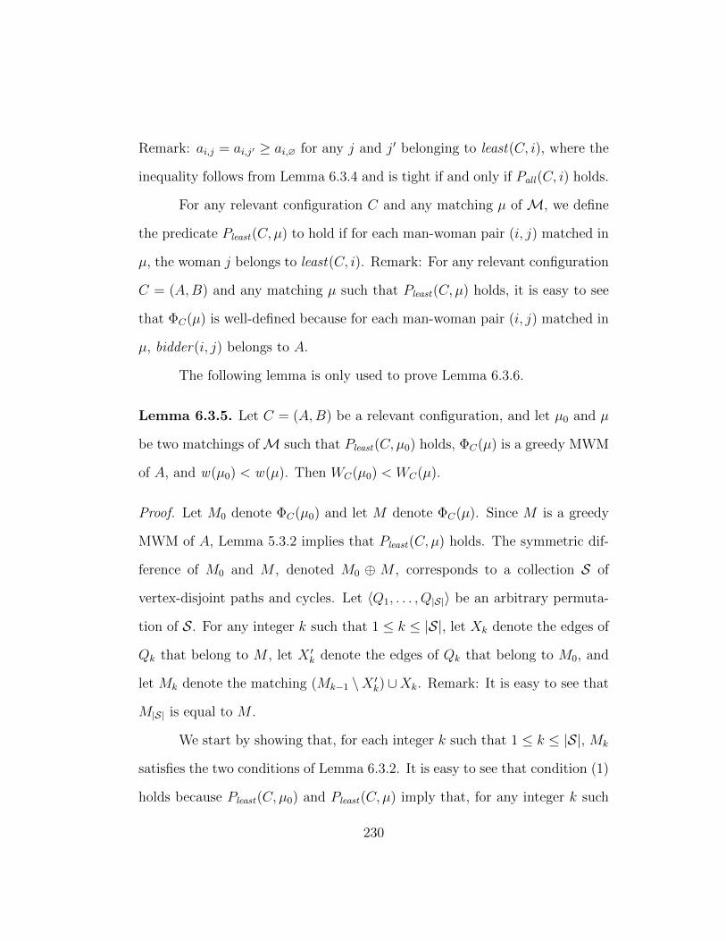
Remark: ai,j = ai,j′ ≥ ai,∅ for any j and j′ belonging to least(C, i), where the

inequality follows from Lemma 6.3.4 and is tight if and only if Pall(C, i) holds.

For any relevant configuration C and any matching µ of M, we define

the predicate Pleast(C, µ) to hold if for each man-woman pair (i, j) matched in

µ, the woman j belongs to least(C, i). Remark: For any relevant configuration

C = (A,B) and any matching µ such that Pleast(C, µ) holds, it is easy to see

that ΦC(µ) is well-defined because for each man-woman pair (i, j) matched in

µ, bidder(i, j) belongs to A.

The following lemma is only used to prove Lemma 6.3.6.

Lemma 6.3.5. Let C = (A,B) be a relevant configuration, and let µ0 and µ

be two matchings ofM such that Pleast(C, µ0) holds, ΦC(µ) is a greedy MWM

of A, and w(µ0) < w(µ). Then WC(µ0) < WC(µ).

Proof. Let M0 denote ΦC(µ0) and let M denote ΦC(µ). Since M is a greedy

MWM of A, Lemma 5.3.2 implies that Pleast(C, µ) holds. The symmetric dif-

ference of M0 and M , denoted M0 ⊕ M , corresponds to a collection S of

vertex-disjoint paths and cycles. Let 〈Q1, . . . , Q|S|〉 be an arbitrary permuta-

tion of S. For any integer k such that 1 ≤ k ≤ |S|, let Xk denote the edges of

Qk that belong to M , let X ′k denote the edges of Qk that belong to M0, and

let Mk denote the matching (Mk−1 \X ′k)∪Xk. Remark: It is easy to see that

M|S| is equal to M .

We start by showing that, for each integer k such that 1 ≤ k ≤ |S|, Mk

satisfies the two conditions of Lemma 6.3.2. It is easy to see that condition (1)

holds because Pleast(C, µ0) and Pleast(C, µ) imply that, for any integer k such

230

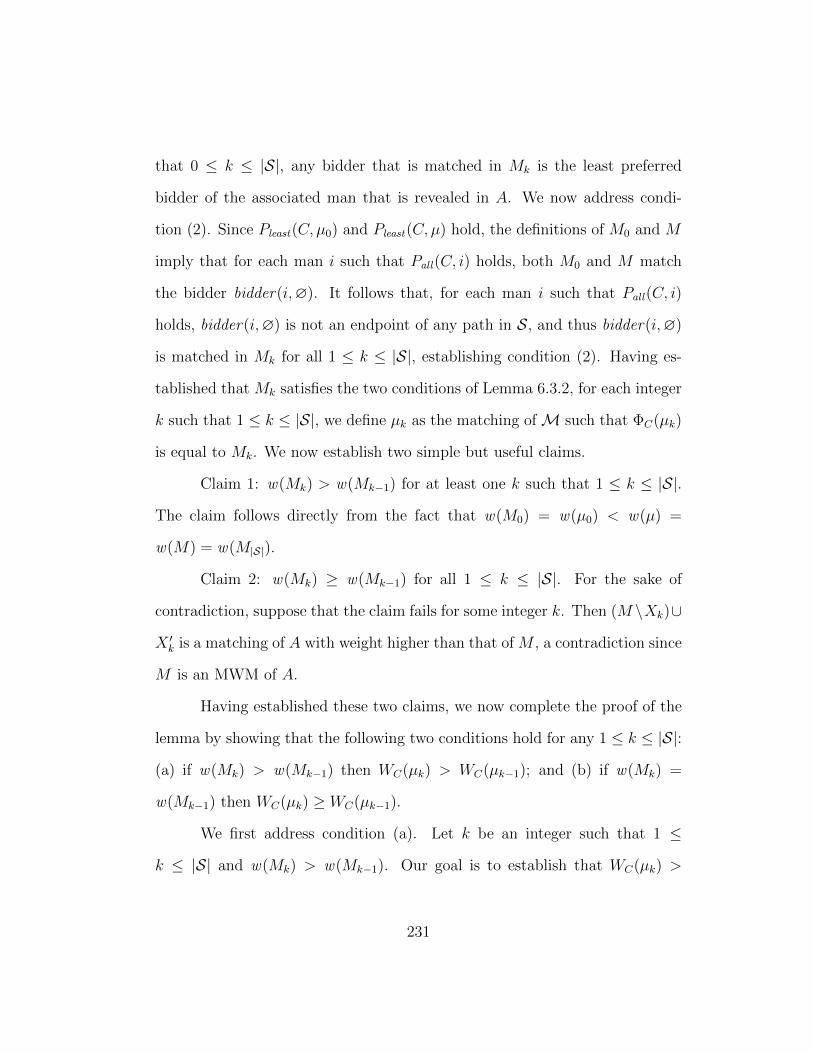
that 0 ≤ k ≤ |S|, any bidder that is matched in Mk is the least preferred

bidder of the associated man that is revealed in A. We now address condi-

tion (2). Since Pleast(C, µ0) and Pleast(C, µ) hold, the definitions of M0 and M

imply that for each man i such that Pall(C, i) holds, both M0 and M match

the bidder bidder(i,∅). It follows that, for each man i such that Pall(C, i)

holds, bidder(i,∅) is not an endpoint of any path in S, and thus bidder(i,∅)

is matched in Mk for all 1 ≤ k ≤ |S|, establishing condition (2). Having es-

tablished that Mk satisfies the two conditions of Lemma 6.3.2, for each integer

k such that 1 ≤ k ≤ |S|, we define µk as the matching ofM such that ΦC(µk)

is equal to Mk. We now establish two simple but useful claims.

Claim 1: w(Mk) > w(Mk−1) for at least one k such that 1 ≤ k ≤ |S|.

The claim follows directly from the fact that w(M0) = w(µ0) < w(µ) =

w(M) = w(M|S|).

Claim 2: w(Mk) ≥ w(Mk−1) for all 1 ≤ k ≤ |S|. For the sake of

contradiction, suppose that the claim fails for some integer k. Then (M \Xk)∪

X ′k is a matching of A with weight higher than that of M , a contradiction since

M is an MWM of A.

Having established these two claims, we now complete the proof of the

lemma by showing that the following two conditions hold for any 1 ≤ k ≤ |S|:

(a) if w(Mk) > w(Mk−1) then WC(µk) > WC(µk−1); and (b) if w(Mk) =

w(Mk−1) then WC(µk) ≥ WC(µk−1).

We first address condition (a). Let k be an integer such that 1 ≤

k ≤ |S| and w(Mk) > w(Mk−1). Our goal is to establish that WC(µk) >

231

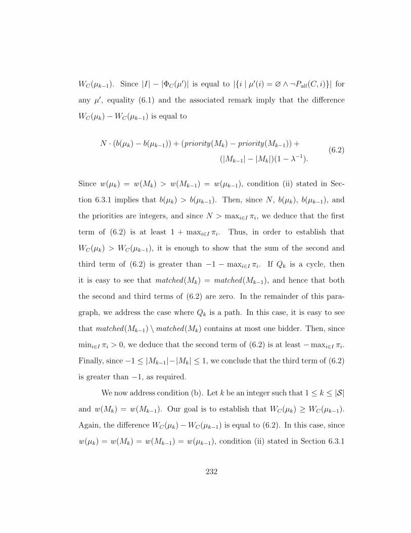
WC(µk−1). Since |I| − |ΦC(µ′)| is equal to |i | µ′(i) = ∅ ∧ ¬Pall(C, i)| for

any µ′, equality (6.1) and the associated remark imply that the difference

WC(µk)−WC(µk−1) is equal to

N · (b(µk)− b(µk−1)) + (priority(Mk)− priority(Mk−1)) +

(|Mk−1| − |Mk|)(1− λ−1).(6.2)

Since w(µk) = w(Mk) > w(Mk−1) = w(µk−1), condition (ii) stated in Sec-

tion 6.3.1 implies that b(µk) > b(µk−1). Then, since N , b(µk), b(µk−1), and

the priorities are integers, and since N > maxi∈I πi, we deduce that the first

term of (6.2) is at least 1 + maxi∈I πi. Thus, in order to establish that

WC(µk) > WC(µk−1), it is enough to show that the sum of the second and

third term of (6.2) is greater than −1 − maxi∈I πi. If Qk is a cycle, then

it is easy to see that matched(Mk) = matched(Mk−1), and hence that both

the second and third terms of (6.2) are zero. In the remainder of this para-

graph, we address the case where Qk is a path. In this case, it is easy to see

that matched(Mk−1) \matched(Mk) contains at most one bidder. Then, since

mini∈I πi > 0, we deduce that the second term of (6.2) is at least −maxi∈I πi.

Finally, since −1 ≤ |Mk−1|−|Mk| ≤ 1, we conclude that the third term of (6.2)

is greater than −1, as required.

We now address condition (b). Let k be an integer such that 1 ≤ k ≤ |S|

and w(Mk) = w(Mk−1). Our goal is to establish that WC(µk) ≥ WC(µk−1).

Again, the difference WC(µk)−WC(µk−1) is equal to (6.2). In this case, since

w(µk) = w(Mk) = w(Mk−1) = w(µk−1), condition (ii) stated in Section 6.3.1

232

implies that b(µk) = b(µk−1), and hence that the first term of (6.2) is zero.

Thus, in order to establish that WC(µk) ≥ WC(µk−1), it remains to show

that the sum of the second and third term of (6.2) is nonnegative. If Qk is a

cycle, then it is easy to see that matched(Mk) = matched(Mk−1), and hence

that both the second and third terms of (6.2) are zero. In the remainder of

this paragraph, we address the case where Qk is a path. In this case, it is

easy to see that matched(Mk) 6= matched(Mk−1). Since (as argued in the

second paragraph of the proof) any bidder that is matched in Mk or in Mk−1

is the least preferred bidder of the associated man that is revealed in A, we

deduce that priority(Mk) 6= priority(Mk−1). We conclude that priority(Mk) >

priority(Mk−1), for otherwise (M \ Xk) ∪ X ′k is an MWM of A with priority

higher than that of M , a contradiction since M is a greedy MWM of A.

It follows that the second term of (6.2) is at least 1 since the priorities are

integers. Finally, since −1 ≤ |Mk−1| − |Mk| ≤ 1, we conclude that the third

term of (6.2) is greater than −1, as required.

Lemma 6.3.6. Let C = (A,B) be a relevant configuration and let X be the

set of all matchings µ of M such that Pleast(C, µ) holds. Let X∗ denote the

set µ | µ ∈ X ∧WC(µ) = maxµ′∈XWC(µ′). Then, ΦC is a bijection from X∗

to the set of greedy MWMs of A.

Proof. Let M be a greedy MWM of A and let µ be the matching (by Lemma

6.3.3) of M such that ΦC(µ) is equal to M . Lemma 5.3.2 implies that

Pleast(C, µ) holds; thus µ belongs to X. Let µ∗ be a matching in X∗ and

let M∗ denote ΦC(µ∗). Note that M∗ is a matching of A. Since ΦC is an

233

injection, it remains to show that WC(µ) = maxµ′∈XWC(µ′) and that M∗ is a

greedy MWM of A.

Since WC(µ) ≤ maxµ′∈XWC(µ′) = WC(µ∗), Lemma 6.3.5 implies that

w(µ) ≤ w(µ∗). Then, since M is an MWM of A, we deduce that M∗ is an

MWM of A. Since M is a greedy MWM, and hence an MCMWM of A, we

deduce that |M∗| ≤ |M |. We consider two cases.

Case 1: |M∗| < |M |. Let x be a bidder in matched(M) \matched(M∗)

such that there exists an MWM, call it M ′, of A having matched(M ′) =

matched(M∗) + x; the exchange property of matroid(A) implies the exis-

tence of such a bidder x and matching M ′. Let i′ denote the man associated

with x. We first argue that M ′ satisfies the two conditions of Lemma 6.3.2.

By definition, the men corresponding to the bidders in matched(M∗) are

distinct; let I ′ denote the set of men corresponding to these bidders, i.e.,

I ′ = i | µ∗(i) 6= ∅ ∨ Pall(C, i). Since Pleast(C, µ∗) holds, we deduce that, for

each man i in I ′, the bidder in matched(M∗) associated with i corresponds to

the least preferred tier of i that is revealed in C. Lemma 5.3.2 implies that x

corresponds to the least preferred tier of i′ that is revealed in C. Then, since

x does not belong to matched(M∗), the results of the preceding two sentences

imply that i′ does not belong to I ′, and thus that M ′ satisfies condition (1).

We now address condition (2). Matching M∗ satisfies condition (2) by def-

inition. Thus M ′ satisfies condition (2) since any bidder matched by M∗ is

also matched by M ′. Since M ′ satisfies conditions (1) and (2), Lemma 6.3.2

implies that there is a matching, call it µ′, of M such that ΦC(µ′) is equal

234

to M ′. Since both M ′ and M∗ are MWMs of A, condition (ii) stated in Sec-

tion 6.3.1 implies that b(µ′) = b(µ∗). Since matched(M ′) properly contains

matched(M∗), we deduce that the set i | µ′(i) 6= ∅ ∨ Pall(C, i) properly con-

tains the set i | µ∗(i) 6= ∅ ∨ Pall(C, i). Then, since πi > (1 − λ−1) for each

man i, the results of the preceding two sentences imply that WC(µ′) > WC(µ∗),

contradicting the definition of µ∗.

Case 2: |M∗| = |M |. Since both M and M∗ are MWMs of A, condi-

tion (ii) stated in Section 6.3.1 implies that b(µ) = b(µ∗). Since |matched(M)| =

|matched(M∗)|, we deduce that the cardinality of i | µ(i) 6= ∅ ∨ Pall(C, i) is

equal to the cardinality of i | µ∗(i) 6= ∅ ∨ Pall(C, i). Then, by using the re-

sults of the preceding two sentences and the remark regarding the second term

in the RHS of (6.1), we deduce that WC(µ) −WC(µ∗) = priority(ΦC(µ)) −

priority(ΦC(µ∗)). The latter expression is nonnegative since M is a greedy

MWM of A, and it is nonpositive since WC(µ∗) = maxµ′∈XWC(µ′). Thus

we deduce that WC(µ) = maxµ′∈XWC(µ′) and that M∗ is a greedy MWM of

A.

6.3.3 Revealing Preferences in the Tiered-Slope Market

Recall that Algorithm 5.1 iteratively reveals the bidders, which correspond

to the tiers of men, and the state of the revealed bidders are captured in a

configuration. In this section, we first show how to adjust the reserve utilities

of the men to obtain markets identical to the tiered-slope market except that

only the tiers that are revealed in a configuration are acceptable (Lemma 6.3.7).

235

Then, we inductively show a bijection (Lemma 6.3.11 and 6.3.14) from the set

of greedy MWMs of the UAP maintained at each iteration of Algorithm 5.1 to

the man-optimal matchings of the corresponding market with adjusted reserve

utilities. Finally, we establish our results in Theorems 6.3.16 and 6.3.17.

For any relevant configuration C, we define reserve(C) as the reserve

utility vector r′ of I such that for each man i,

r′i = maxri, (1− λ−1) expλ(ai,j)

=

πi expλ(ai,∅) if Pall(C, i)

(1− λ−1) expλ(ai,j) otherwise,

where j is some element in least(C, i).

For any reserve utility vector r′ of I such that r′ ≥ r, we define M(r′)

as the market that is equal to M except that the reserve utilities of the

men are given by r′. For any relevant configuration C, we define M(C) as

M(reserve(C)). Lemma 6.3.7 below shows that, for any relevant configuration

C, only the tiers of men that are revealed in C are “acceptable” in M(C).

Lemma 6.3.7. Let C = (A,B) be a relevant configuration, let (µ, u, v) be an

individually rational outcome for M(C), and let (i, j) be a man-woman pair

matched in µ. Then bidder(i, j) belongs to A.

236

Proof. We have

fi,j(ui) ≤ −gi,j(vj) = −vj +Nbi,j + πi

≤ N (bi,j − b∅,j) + πi

≤ Nbi,j −N + πi

≤ λ− 2N + πi

≤ λ− 2,

where the inequalities are justified as follows: the first inequality follows from

the feasibility of (µ, u, v); the second inequality follows from the individual

rationality of (µ, u, v), which implies vj ≥ sj = Nb∅,j; the third inequality

follows since b∅,j ≥ 1; the fourth inequality follows since λ ≥ maxi,j(bi,j +1)N ;

the fifth inequality follows since N > maxi∈I πi. Then, since fi,j(ui) ≤ λ − 2,

we deduce that ui ≤ (λ− 2) expλ(ai,j).

Let r′ denote reserve(C) and let j′ be an arbitrary element in least(C, i).

Assume the claim of the lemma is false: thus ai,j < ai,j′ . Then, since ui ≤

(λ− 2) expλ(ai,j), we conclude that ui < (1− λ−1) expλ(ai,j′), and hence that

ui < r′i, contradicting individual rationality.

The following lemma provides a lower bound on the utilities of men in

the man-optimal outcomes. It is used in the proof of Lemma 6.3.14.

Lemma 6.3.8. Let C be a relevant configuration, let (µ, u, v) be a man-

optimal outcome forM(C), and let (i, j) be a man-woman pair matched in µ.

Then ui ≥ expλ(ai,j).

237

Proof. Let r′ denote reserve(C). We show that r′ satisfies the conditions re-

quired by Lemma 6.1.2, then the claim follows from that lemma. By definition,

r′ is at least r, so it satisfies condition (i). For any man i, if Pall(C, i) holds,

then r′i is equal to πi expλ(ai,∅), and it is easy to see that r′i expλ(k) is an

integer for any integer k ≥ −ai,∅ and that 0 < r′i expλ(k) < 1 for any integer

k < −ai,∅; otherwise, r′i is equal to (1−λ−1) expλ(ai,j) where j is some element

in least(C, i), and it is easy to see that r′i expλ(k) is an integer for any integer

k > −ai,j and that 0 < r′i expλ(k) < 1 for any integer k ≤ −ai,j. Thus, r′

satisfies condition (ii) as well.

For a matching µ satisfying Pleast(C, µ), the following lemma gives a

necessary and sufficient condition for µ to be a stable matching ofM(C). The

proof of the lemma is quite involved and is deferred to Section 6.3.4.

Lemma 6.3.9. Let C be a relevant configuration and let X be the set of all

matchings µ of M(C) such that Pleast(C, µ) holds. Assume that there exists

at least one stable outcome, denoted (µ, u, v), for M(C) such that µ belongs

to X. Then, a matching µ∗ that belongs to X is compatible with the stable

payoff (u, v) if and only if WC(µ∗) = maxµ′∈XWC(µ′).

For any relevant configuration C, we define the predicate Popt(C) to hold

if for each man-optimal matching µ of M(C), Pleast(C, µ) holds. Remark: It

is easy to see that Pleast(C1, µ) holds for any matching µ of M(C1), and thus

Popt(C1) holds. For a relevant configuration C satisfying Popt(C), the following

lemma characterizes the man-optimal matchings of M(C).

238

Lemma 6.3.10. Let C be a relevant configuration such that Popt(C) holds.

Let X be the set of all matchings µ ofM(C) such that Pleast(C, µ) holds. Then,

a matching µ is a man-optimal matching of M(C) if and only if µ belongs to

X and WC(µ) = maxµ′∈XWC(µ′).

Proof. Let X∗ denote the set µ | µ ∈ X ∧WC(µ) = maxµ′∈XWC(µ′). Since

Popt(C) implies that all man-optimal matchings of M(C) are included in X,

and since there is at least one man-optimal matching [14, Property 2], we

deduce that X contains a man-optimal, and hence stable, matching. Thus,

Lemma 6.3.9 implies that the set of stable matchings ofM(C) is equal to X∗,

and that each matching in X∗ is compatible with the man-optimal payoff in

M(C).

Lemma 6.3.11. Let C = (A,B) be a relevant configuration such that Popt(C)

holds. Then, ΦC is a bijection from the set of man-optimal matchings ofM(C)

to the set of greedy MWMs of A.

Proof. Let X be the set of all matchings M(C) of M such that Pleast(C, µ)

holds. LetX∗ denote the set µ | µ ∈ X ∧WC(µ) = maxµ′∈XWC(µ′). Lemma

6.3.10 implies that the set of man-optimal matchings ofM(C) is equal to X∗.

Then the claim follows from Lemma 6.3.6.

Having established the correspondence between the man-optimal match-

ings and the greedy MWMs given a relevant configuration C such that Popt(C)

holds, we now show inductively in Lemma 6.3.14 that Popt(C) holds for all rel-

evant configurations C. We start with two lemmas that are useful in proving

239

Lemma 6.3.14; the second one (Lemma 6.3.13) is also used in the proof of

Theorem 6.3.16.

Lemma 6.3.12. Let C be a relevant configuration such that Popt(C) holds, let

r′ denote reserve(C), and let (u, v) denote the man-optimal payoff in M(C).

Then, for each bidder in ready(C), we have ui = r′i, where i denotes the man

associated with that bidder.

Proof. Let C be (A,B). If a bidder belongs to ready(C), then it is not matched

in any greedy MWM of A, and the definition of ΦC and Lemma 6.3.11 imply

that it is not matched in any man-optimal matching ofM(C). Then the claim

of the lemma follows from the stability of (u, v).

Lemma 6.3.13. Let r′ and r′′ be two reserve utility vectors of the men such

that r′ ≥ r′′ ≥ r. Let (u′, v′) and (u′′, v′′) be the man-optimal payoffs ofM(r′)

and M(r′′), respectively. Then u′ ≥ u′′.

Proof. The claim of the lemma follows directly from [14, Property 3].

Lemma 6.3.14. Let C be a relevant configuration such that for each relevant

configuration C ′ that precedes C, Popt(C′) holds. Then Popt(C) holds.

Proof. Consider an arbitrary canonical execution that produces C at some

iteration and let (A,B) be the configuration C. For the sake of contradiction,

assume Popt(C) does not hold. Let (µ, u, v) be a man-optimal outcome for

M(C) such that Pleast(C, µ) does not hold and let (i, j) be a man-woman

pair matched in µ such that j does not belong to least(C, i). Let j′ be an

240

arbitrary element of least(C, i). Since Lemma 6.3.7 implies that bidder(i, j)

belongs to A, we deduce that ai,j > ai,j′ . Let C ′ be the configuration at the

beginning of the iteration that reveals the tier of i corresponding to least(C, i),

i.e., the iteration at which bidder(i, j′) is added at line 4 of Algorithm 5.1. Let

j′′ be an arbitrary element of least(C ′, i), let r′ denote reserve(C ′), and let

(u′, v′) denote the man-optimal payoff inM(C ′). Then, we deduce that ai,j ≥

ai,j′′ > ai,j′ ≥ ai,∅, where the last inequality follows from Lemma 6.3.4. Thus,

Pall(C′, i) does not hold, and hence r′i = (1−λ−1) expλ(ai,j′′). Since bidder(i, j′)

belongs to ready(C ′), and since Popt(C′) holds, Lemma 6.3.12 implies that

u′i = r′i = (1− λ−1) expλ(ai,j′′). On the other hand, since the man-woman pair

(i, j) is matched in µ, which is a man-optimal matching ofM(C), Lemma 6.3.8

implies that ui ≥ expλ(ai,j). Combining the results of the preceding two

sentences, we conclude that ui ≥ expλ(ai,j) > (1 − λ−1) expλ(ai,j′′) = u′i,

contradicting Lemma 6.3.13 since reserve(C) ≤ reserve(C ′).

We are now ready to establish our equivalence result in Theorem 6.3.16

and the group strategyproofness result in Theorem 6.3.17. We start with a

useful lemma.

Lemma 6.3.15. For each greedy MWM M of uap(B) and each man i, some

bidder associated with i is matched in M .

Proof. Suppose the claim does not hold, and let M be a greedy MWM of

uap(B) and let i be a man such that no bidder associated with i is matched

in M . Then all of the bidders associated with i belong to uap(B), for oth-

erwise ready(CF ) is nonempty, contradicting the definition of CF (recall that

241

CF = (uap(B), B) is the unique final configuration of any canonical execu-

tion). Thus, we deduce that Pall(CF , i) holds, and Lemma 6.3.1 implies that

some bidder associated with i is matched in M , a contradiction.

Theorem 6.3.16. ΦCFis a bijection from the set of man-optimal matchings

of M to the set of greedy MWMs of uap(B).

Proof. Observe that Popt(CF ) holds by repeated application of Lemma 6.3.14.

Let (u, v) denote the man-optimal payoff inM(CF ). Let r′ denote reserve(CF )

and recall that r is the reserve utility vector of the men inM. We now prove

two useful claims.

Claim 1: Any man-optimal outcome (µ, u, v) for M(CF ) is stable for

M. Let (µ, u, v) be a man-optimal outcome for M(CF ). Since M(CF ) and

M differ only in the reserve utility vectors of the men, it is enough to show

that for each man i who is unmatched in µ, we have ui = ri. Let i be a man

who is unmatched in µ. Observe that Pall(CF , i) holds, for otherwise no bidder

associated with i is matched in ΦCF(µ), which is a greedy MWM of uap(B)

by Lemma 6.3.11, contradicting Lemma 6.3.15. Thus r′i = πi expλ(ai,∅) = ri.

Then, by the stability of (µ, u, v) for M(CF ), we conclude that ui = r′i = ri.

Claim 2: Any man-optimal outcome forM is stable forM(CF ). Claim

1 and Lemma 6.3.13 imply that the payoff (u, v), which is the man-optimal

payoff in M(CF ), is also the man-optimal payoff in M. Let (µ, u, v) be a

man-optimal outcome for M. As in the proof of Claim 1, since M(CF ) and

M differ only in the reserve utility vectors of the men, it is enough to show

that for each man i who is unmatched in µ, we have ui = r′i. Let i be a man

242

who is unmatched in µ. By the stability of (µ, u, v) for M, we deduce that

ui = ri. By the individual rationality of (u, v) for M(CF ), we deduce that

ui ≥ r′i. Since r′ ≥ r, we conclude that ui = ri = r′i.

Claims 1 and 2, and Lemma 6.3.13 imply that the set of man-optimal

matchings ofM is equal to the set of man-optimal matchings ofM(CF ). Then

the theorem follows from Lemma 6.3.11 since Popt(CF ) holds.

Theorem 6.3.17. The SMIW mechanism of Section 5.4 is group strate-

gyproof.

Proof. As we mentioned in Section 6.2, Algorithm 6.1 implements the mech-

anism of Section 5.4. Given an instance of the stable marriage market with

indifferences, if we construct a tiered-slope market M associated with this

instance and we run Algorithm 6.1 by setting the edge weights as described in

Section 6.3.1, Theorem 6.3.16 implies that the output corresponds to a man-

optimal matching of M. Then the result follows from Theorem 6.1.1.

6.3.4 Proof of Lemma 6.3.9

The purpose of this section is to prove Lemma 6.3.9. We start with some

useful lemmas.

Lemma 6.3.18. Let C be a relevant configuration, let µ be a matching of

M(C), and let v be a utility vector of the women such that vj = sj for each

243

woman j who is unmatched in µ. Then,

∑j∈J

vj −WC(µ) + π∅(C, µ) =∑

µ(j)6=∅

gµ(j),j(vj).

Proof.

∑j∈J

vj −WC(µ) + π∅(C, µ) =∑j∈J

vj −N · b(µ)−∑µ(i) 6=∅

πi

=∑

µ(j) 6=∅

vj −N∑

µ(j)6=∅

bµ(j),j −∑

µ(j)6=∅

πµ(j)

+∑

µ(j)=∅

sj −N∑

µ(j)=∅

b∅,j

=∑

µ(j) 6=∅

(vj − bµ(j),jN − πµ(j)

)=∑

µ(j) 6=∅

gµ(j),j(vj),

where the third equality follows since sj = Nb∅,j.

Lemma 6.3.19. Let C be a relevant configuration and let (µ, u, v) be a stable

outcome for M(C). Then,

WC(µ) =∑µ(i)6=∅

fi,µ(i)(ui) +∑j∈J

vj + π∅(C, µ).

Proof. The stability and feasibility of (µ, u, v) imply that fi,j(ui) + gi,j(vj) =

0 for each man-woman pair (i, j) matched in µ. Thus,∑

µ(i)6=∅ fi,µ(i)(ui) +∑µ(j)6=∅ gµ(j),j(vj) = 0, and the claim follows from Lemma 6.3.18, since the

244

stability of (µ, u, v) implies that vj = sj for each woman j who is unmatched

in µ.

Lemma 6.3.20. Let C be a relevant configuration, let µ and µ′ be two match-

ings such that Pleast(C, µ) and Pleast(C, µ′) hold, let r′ denote reserve(C), and

let u be a utility vector such that for each man i, ui = r′i if µ(i) = ∅ or

µ′(i) = ∅. Then∑

µ(i)6=∅ fi,µ(i)(ui)+π∅(C, µ) =∑

µ′(i) 6=∅ fi,µ′(i)(ui)+π∅(C, µ′).

Proof. Let fi,∅(ui) denote 0. We show that fi,µ(i)(ui)+π∅(C, µ, i) = fi,µ′(i)(ui)+

π∅(C, µ′, i) for each man i. Let i be an arbitrary man. We consider six cases.

Case 1: µ(i) 6= ∅ and µ′(i) 6= ∅. Then π∅(C, µ, i) = π∅(C, µ′, i) =

0. Pleast(C, µ) and Pleast(C, µ′) and imply that ai,µ(i) = ai,µ′(i), and hence

fi,µ(i)(ui) = fi,µ′(i)(ui).

Case 2: µ(i) = µ′(i) = ∅. In this case π∅(C, µ, i) (resp., π∅(C, µ′, i)) is

independent of µ (resp., µ′).

Case 3 (resp., case 4): µ(i) 6= ∅ and µ′(i) = ∅ (resp., µ(i) = ∅

and µ′(i) 6= ∅) and Pall(C, i). Since Pall(C, i) holds, we deduce that r′i =

πi expλ(ai,∅). Then, since ui = r′i, Pleast(C, µ) (resp., Pleast(C, µ′)) implies

that fi,µ(i)(ui) + π∅(C, µ, i) = fi,µ(i)(r′i) = πi (resp., fi,µ′(i)(ui) + π∅(C, µ′, i) =

fi,µ′(i)(r′i) = πi). Since µ′(i) = ∅ (resp., µ(i) = ∅), we deduce that fi,µ′(i)(ui)+

π∅(C, µ′, i) (resp., fi,µ(i)(ui) + π∅(C, µ, i)) is equal to 0 + πi = πi.

Case 5 (resp., case 6): µ(i) 6= ∅ and µ′(i) = ∅ (resp., µ(i) = ∅ and

µ′(i) 6= ∅) and ¬Pall(C, i). Let j denote µ(i) (resp., µ′(i)). Since Pleast(C, µ)

(resp., Pleast(C, µ′)) and ¬Pall(C, i), we deduce that r′i = (1 − λ−1) expλ(ai,j).

Then, since ui = r′i, we deduce that fi,µ(i)(ui) + π∅(C, µ, i) = fi,µ(i)(r′i) =

245

(1 − λ−1) (resp., fi,µ′(i)(ui) + π∅(C, µ′, i) = fi,µ′(i)(r′i) = (1 − λ−1)). Since

µ′(i) = ∅ (resp., µ(i) = ∅), we deduce that fi,µ′(i)(ui) + π∅(C, µ′, i) (resp.,

fi,µ(i)(ui) + π∅(C, µ, i)) is equal to 0 + (1− λ−1) = (1− λ−1).

Lemma 6.3.21. Let C be a relevant configuration and let r′ denote reserve(C).

Let X be the set of all matchings µ ofM(C) such that Pleast(C, µ) holds. Let

(µ, u, v) be a stable outcome for M(C) such that µ belongs to X. Let µ∗

be a matching in X such that WC(µ∗) = maxµ′∈XWC(µ′). Then the follow-

ing claims hold: (1) ui = r′i if µ∗(i) = ∅; (2) vj = sj if µ∗(j) = ∅; (3)∑µ(i)6=∅ fi,µ(i)(ui) + π∅(C, µ) =

∑µ∗(i)6=∅ fi,µ∗(i)(ui) + π∅(C, µ∗).

Proof. Let S denote the symmetric difference of µ and µ∗. It is easy to see

that S is a collection of positive length paths and cycles. In order to prove

Claim (1) of the lemma, consider an arbitrary man i such that µ∗(i) = ∅.

If µ(i) = ∅, then the stability of (u, v) establishes the claim, so assume that

µ(i) 6= ∅. Then, i is an endpoint of a path in S; let P denote this path. The

edges of P alternate between edges that are matched in µ and edges that are

matched in µ∗. We consider two cases.

Case 1: The other endpoint of P is a man i′ such that µ(i′) = ∅ and

µ∗(i) 6= ∅. Let P be 〈i = i1, j1, . . . , jk, ik+1 = i′〉 for some k ≥ 1. Then, since

µ(i`) = j` for 1 ≤ ` ≤ k, the stability of (µ, u, v) implies that

∑1≤`≤k

[fi`,j`(ui`) + gi`,j`(vj`)] = 0.

246

The stability of (µ, u, v) also implies that

∑1≤`≤k

[fi`+1,j`(ui`+1

) + gi`+1,j`(vj`)]≥ 0.

By subtracting the latter equation from the former, we obtain the following,

since Pleast(C, µ) and Pleast(C, µ∗) imply fi`,j`(ui`) = fi`,j`−1

(ui`) for 1 < ` ≤ k:

0 ≥ fi,j1(ui)− fi′,jk(ui′) +∑

1≤`≤k

[gi`,j`(vj`)− gi`+1,j`(vj`)

]= (fi,j1(ui)− πi)− (fi′,jk(ui′)− πi′) +N

∑1≤`≤k

(bi`+1,j` − bi`,j`

). (6.3)

Observe that

fi,j1(ui)− πi ≥ fi,j1(r′i)− πi ≥ (1− λ−1)− πi > −N, (6.4)

since the individual rationality of (u, v) implies ui ≥ r′i and since Pleast(C, µ)

holds. Also observe that

fi′,jk(ui′)− πi′ = fi′,jk(r′i′)− πi′ ≤ 0,

since the stability of (µ, u, v) implies ui′ = r′i′ and since Pleast(C, µ∗) holds.

These two observations imply that the third term in (6.3) is nonpositive, for

otherwise it would be at least N (since all b values are integers), violating the

inequality. The third term in (6.3) is nonnegative, for otherwise µ∗ could be

augmented along P to yield another matching µ′ such that Pleast(C, µ′) and

247

WC(µ′)−WC(µ∗) ≥ N − πi′ > 0 (since all b values are integers and N > πi′),

contradicting the definition of µ∗. Thus, we may rewrite inequality (6.3) as

fi′,jk(r′i′)− πi′ ≥ fi,j1(ui)− πi. (6.5)

We consider the following four subcases.

Case 1.1: Pall(C, i) and Pall(C, i′). Since Pleast(C, µ

∗) and Pall(C, i′)

hold, we deduce that r′i′ = πi′ expλ(ai′,jk), and hence that LHS of (6.5) is 0.

Since Pleast(C, µ) and Pall(C, i) hold, we deduce that r′i = πi expλ(ai′,j1), and

hence that RHS of (6.5) is at least 0 by the first inequality of (6.4). Thus, we

conclude that fi,j1(ui) = πi, which implies ui = r′i.

Case 1.2: ¬Pall(C, i) and ¬Pall(C, i′). First observe that πi′ > πi, for

otherwise µ∗ could be augmented along P to yield another matching µ′ such

that Pleast(C, µ′) and WC(µ′) − WC(µ∗) = πi − πi′ > 0, contradicting the

definition of µ∗. Since Pleast(C, µ∗) holds and Pall(C, i

′) does not hold, we

deduce that r′i′ = (1 − λ−1) expλ(ai′,jk), and hence that LHS of (6.5) is (1 −

λ−1) − πi′ . However, the RHS of (6.5) is at least (1 − λ−1) − πi by (6.4),

contradicting the inequality πi′ > πi.

Case 1.3: ¬Pall(C, i) and Pall(C, i′). This case is not possible, for oth-

erwise µ∗ could be augmented along P to yield another matching µ′ such that

Pleast(C, µ′) and WC(µ′)−WC(µ∗) = πi − (1− λ−1) > 0 (since πi > (1− λ−1)

for each man i), contradicting the definition of µ∗.

Case 1.4: Pall(C, i) and ¬Pall(C, i′). Since Pleast(C, µ

∗) holds and Pall(C, i′)

does not hold, we deduce that r′i′ = (1−λ−1) expλ(ai′,jk), and hence that LHS

248

of (6.5) is (1− λ−1)− πi′ < 0. Since Pleast(C, µ) and Pall(C, i) hold, we deduce

that r′i = πi expλ(ai′,j1), and hence that RHS of (6.5) is at least 0 by the first

inequality of (6.4), a contradiction.

Case 2: The other endpoint of P is a woman j such that µ(j) 6= ∅ and

µ∗(j) = ∅. Let P be 〈i = i1, j1, . . . , ik, jk = j〉 for some k ≥ 1. Then, since

µ(i`) = j` for 1 ≤ ` ≤ k, the stability of (µ, u, v) implies that

∑1≤`≤k

[fi`,j`(ui`) + gi`,j`(vj`)] = 0.


∑1<`≤k

[fi`,j`−1

(ui`) + gi`,j`−1(vj`−1

)]≥ 0.


since Pleast(C, µ) and Pleast(C, µ∗) imply fi`,j`(ui`) = fi`,j`−1

(ui`) for 1 < ` ≤ k:

0 ≥ fi,j1(ui) +∑

1≤`≤k

gi`,j`(vj`)−∑

1<`≤k

gi`,j`−1(vj`−1

)

= (fi,j1(ui)− πi) + vj +N

[ ∑1<`≤k

bi`,j`−1−∑

1≤`≤k

bi`,j`

]

= (fi,j1(ui)− πi) + (vj − sj) +N

[(b∅,j +

∑1<`≤k

bi`,j`−1

)−∑

1≤`≤k

bi`,j`

].

(6.6)

Observe that (6.4) holds for the same reasons pointed out in Case 1, and

that the second term in (6.6) is nonnegative by the individual rationality of

249

(u, v). Moreover, the third term is nonnegative, for otherwise µ∗ could be

augmented along P to yield another matching µ′ such that Pleast(C, µ′) and

WC(µ′) − WC(µ∗) ≥ N (since all b values are integers), contradicting the

definition of µ∗. We consider two subcases.

Case 2.1: Pall(C, i). Then Pleast(C, µ) implies that r′i = πi expλ(ai′,j1),

and we deduce that the first term in (6.6) is at least 0 by the first inequality

of (6.4). Thus, we conclude that vj = sj and that fi,j1(ui) = πi, which implies

ui = r′i.

Case 2.2: ¬Pall(C, i). In this case the third term in (6.6) is positive,

and thus is at least N (since all b values are integers), for otherwise (if it is

0), µ∗ could be augmented along P to yield another matching µ′ such that

Pleast(C, µ′) and WC(µ′) − WC(µ∗) = πi − (1 − λ−1) > 0, contradicting the

definition of µ∗. Since (6.4) implies that the first term of (6.6) is greater

than −N , we deduce that the sum of the three terms in (6.6) is positive, a

contradiction.

In order to prove Claim (2) of the lemma, consider an arbitrary woman

j such that µ∗(j) = ∅. If µ(j) = ∅, then the stability of (u, v) establishes the

claim, so assume that µ(j) 6= ∅. Then, j is an endpoint of a path in S; let P

denote this path. The edges of P alternate between edges that are matched

in µ and edges that are matched in µ∗. We consider two cases.

Case 1: The other endpoint of P is a woman j′ such that µ(j′) = ∅

and µ∗(j) 6= ∅. Let P be 〈j = j1, i1, . . . , ik, jk+1 = j′〉 for some k ≥ 1. Then,

250

since µ(i`) = j` for 1 ≤ ` ≤ k, the stability of (µ, u, v) implies that

∑1≤`≤k

[fi`,j`(ui`) + gi`,j`(vj`)] = 0.


∑1≤`≤k

[fi`,j`+1

(ui`) + gi`,j`+1(vj`+1

)]≥ 0.


since Pleast(C, µ) and Pleast(C, µ∗) imply fi`,j`(ui`) = fi`,j`+1

(ui`) for 1 ≤ ` ≤ k:

0 ≥∑

1≤`≤k

[gi`,j`(vj`)− gi`,j`+1

(vj`+1)]

= vj − vj′ +N∑

1≤`≤k

(bi`,j`+1

− bi`,j`)

= (vj − sj) +N

[(b∅,j +

∑1≤`≤k

bi`,j`+1

)−

(b∅,j′ +

∑1≤`≤k

bi`,j`

)], (6.7)

where the last equality follows since µ(j′) = ∅ implies vj′ = sj′ = b∅,j′N . The

first term in (6.7) is nonnegative by the individual rationality of (u, v). The

second term is nonnegative, for otherwise µ∗ could be augmented along P to

yield another matching µ′ such that Pleast(C, µ′) and WC(µ′) −WC(µ∗) ≥ N

(since all b values are integers), contradicting the definition of µ∗. Thus, we

conclude that vj = sj.

Case 2: The other endpoint of P is a man i such that µ(i) 6= ∅ and

µ∗(i) = ∅. This case is identical to case 2 in the proof of Claim (1) above,

251

and hence we conclude that vj = sj.

We now prove Claim (3) of the lemma. Stability of (µ, u, v) implies ui =

r′i if µ(i) = ∅. Thus Claim (3) follows using Claim (1) and Lemma 6.3.20.

Proof of Lemma 6.3.9. Let µ∗ be a matching in X such that WC(µ∗) is equal

to maxµ′∈XWC(µ′). We show that WC(µ) = WC(µ∗) and that µ∗ is compatible

with the stable payoff (u, v). We have

WC(µ∗) ≥ WC(µ) =∑µ(i)6=∅

fi,µ(i)(ui) +∑j∈J

vj + π∅(C, µ)

=∑

µ∗(i)6=∅

fi,µ∗(i)(ui) +∑j∈J

vj + π∅(C, µ∗), (6.8)

where the first equality follows from Lemma 6.3.19, and the second equal-

ity follows from Claim (3) of Lemma 6.3.21. Then, by using Claim (2) of

Lemma 6.3.21 and Lemma 6.3.18, we may rewrite (6.8) as

0 ≥∑

µ∗(i)6=∅

fi,µ∗(i)(ui) +∑

µ∗(j)6=∅

gµ∗(j),j(vj) =∑

µ∗(i)=j∧j 6=∅

[fi,j(ui) + gi,j(vj)] .

(6.9)

Then, since the stability of (u, v) implies that fi,j(ui) + gi,j(vj) ≥ 0 for each

man-woman pair (i, j), we deduce the following: the inequality of (6.9) is tight,

and hence that of (6.8) is also tight; fi,j(ui)+gi,j(vj) = 0 for each man-woman

pair (i, j) matched in µ∗. Thus, Claims (1) and (2) of Lemma 6.3.21 imply

that µ∗ is compatible with the stable payoff (u, v).

252

Chapter 7

Concluding Remarks

The main contributions of this dissertation are fast algorithms for implement-

ing the VCG mechanism for certain compactly representable special cases of

unit-demand auctions, and a group strategyproof Pareto-stable mechanism for

the stable marriage model with incomplete and weak preferences (SMIW). The

latter mechanism is the first strategyproof and Pareto-stable mechanism for

SMIW. This mechanism is developed using a framework based on two variants

of unit-demand auctions, namely UAPs and IUAPs, which allow us to gener-

alize the well-known deferred acceptance algorithm. We have established the

group strategyproofness of the mechanism by showing that it coincides with

the more recent group strategyproof Pareto-stable mechanism (for the same

model) of Domanic et al. [17].

A number of questions arise naturally given the results of this disserta-

tion and the techniques used to derive these results. In this chapter, we state

several questions that are of potential interest for future research.

253

7.1 Further Variants of UDALEWs

We studied the problem of computing a VCG outcome of a UDALEW in

Chapter 2, and we studied two special cases of UDALEWs in Chapter 4.

These special cases are motivated by applications to the scheduling domain,

and enable us to solve two variants of the problem of scheduling unit jobs with

rejection in O(n log n) time. The (more general) UDALEWs can be used to

solve other variants of this problem, for instance the problem of scheduling

(with rejection) unit jobs having symmetric earliness and tardiness penalties

with respect to a common due date, but the algorithm that we present in Chap-

ter 2 is not as fast as the O(n log n)-time algorithms of Chapter 4. One can

investigate further special cases of UDALEWs that allow for algorithms faster

than that of Chapter 2. For instance, solving the special case of UDALEWs

where the item qualities form the sequence 〈1, 1, 2, 2, . . . , d, d〉 addresses the

aforementioned variant of the problem with symmetric earliness and tardiness

penalties with respect to a common due date.1

One can investigate further generalizations of UDALEWs that allow for

efficient algorithms for computing a VCG outcome. One can seek applications

1It can be shown that the acceptance order notion of Section 4.2.1 is also well-defined inthis special case, so one can hope to follow the footsteps of Section 4.2 to devise an algorithmfor this case. Let us see what happens if we try to apply the techniques of Section 4.2.2to compute the acceptance orders. Consider the example illustrated in Figure 4.1, in whichwe try to determine whether the job with index 10 precedes σ9[7] in σ10. Imagine thatthe slots now have “qualities” that form the sequence 〈1, 1, 2, 2, . . .〉; the qualities are notdepicted explicitly in the figure because the indices of the slots played the role of qualitiesin the model of Section 4.2. The approach of comparing the weights of two matchings,as illustrated in Figure 4.1b, fails because only some of the jobs, instead of all, in the setbest(9, 6) \ better(σ9[7]) are shifted to a slot that have one lower “quality”.

254

and algorithms for the models that incorporate one, or a combination, of the

following to UDALEWs: a budget constraint with each unit-demand bid; a

lower or an upper bound on the qualities of the items that is acceptable for

each unit-demand bid; a quality threshold with each unit-demand bid so that

the offer is given by an affine function up to the threshold, and is a constant

after the threshold; vectors of fixed dimensions to play the role of bid slopes

and item qualities (in this case the offer is the intercept plus the dot product

of the slope and the quality); the operation of removing a unit-demand bid

from the auction.

7.2 Further Applications and Generalizations

of IUAPs

In Sections 5.2 and 5.3, we introduced the UAPs and IUAPs, and we pre-

sented a framework based on these two variants of unit-demand auctions for

generalizing the deferred acceptance algorithm. One can investigate further

applications and generalizations of UAPs, IUAPs, and this framework. In Sec-

tion 5.4.1, we described how we exploit our framework to devise a Pareto-stable

and group strategyproof mechanism for SMIW; however, in this application,

the IUAP mechanism is invoked in a somewhat unusual manner, in that the

offers appearing in the unit-demand bids of the multibidder corresponding to

a man i are determined by the women — i only gets to determine the set of

women to be included in each unit-demand bid in his bid sequence. A pos-

255

sible direction for further investigation is to seek more direct applications of

IUAPs, e.g., to implement mechanisms in a variant of unit-demand auctions

that incorporates budget constraints into each unit-demand bid [4, 22]. An-

other possible direction is to generalize the UAPs and IUAPs further, e.g., to

allow each component of a unit-demand bid to specify a piecewise linear utility

function, instead of a single valuation, as in the work of Dutting et al. [21].

7.3 Threshold Prices and Group Strategyproof-

ness

We established the strategyproofness of our mechanism by utilizing the notion

of threshold prices in IUAPs. However, our proof of group strategyproofness

in Chapter 6 did not rely on this notion. Instead, we showed that it coincides

with a more recent group strategyproof Pareto-stable mechanism. One can

investigate whether it is possible to directly establish group strategyproofness

by generalizing the notion of threshold prices to a group of items and by

generalizing the related lemma (Lemma 5.3.8) to a group of multibidders. In

this regard, a plausible approach is to delay the introduction of any unit-

demand bids of a group of multibidders until the members of that group are

the sole unmatched multibidders whose sequences of unit-demand bids have

not been exhausted. One can then seek to characterize the utilities that the

members of the group would obtain from any sequence of unit-demand bids

that they might choose to submit.

256


A number of interesting questions related to the stable marriage model with

indifferences arise naturally given the existence of various stability notions

and other game-theoretic properties of interest. Here we give some examples

of these questions.

Recall that we mentioned three stability notions in Section 1.2 regard-

ing the stable marriage model when indifferences are allowed: weak stability,

strong stability, and super-stability. Our mechanism returns a weakly stable

matching. One can investigate whether any of the other stability notions is

achievable by a Pareto-optimal and (group) strategyproof mechanism. Here

we briefly review the notion of strong stability. We say that a man i and a

woman j form a weakly blocking pair with respect to a matching M if (1) i

weakly prefers j to his match in M , (2) j weakly prefers i to her match in

M , and (3) either (3a) i prefers j to his match in M or (3b) j prefers i to her

match in M . A matching that does not admit a weakly blocking pair is said to

be strongly stable. Unfortunately, it is not difficult to exhibit SMCW instances

for which the set of strongly stable matchings is empty (see, e.g., Manlove [42,

Section 3.3.1]). For SMIW instances that admit a strongly stable matching,

it is desirable for the mechanism to return a matching that is Pareto-optimal

and strongly stable. Does our mechanism achieve this property? If not, can

we extend it to do so? Can we provide a (partial) characterization of the

class of strategyproof (resp., group strategyproof) mechanisms for computing

a Pareto-stable matching? Is every strategyproof Pareto-stable mechanism for

257

SMIW also group strategyproof?

258

Bibliography

[1] Canadian resident matching service. URL http://carms.ca/.

[2] A. Abdulkadiroglu, P. A. Pathak, and A. E. Roth. Strategy-proofness

versus efficiency in matching with indifferences: redesigning the NYC

high school match. The American Economic Review, 99:1954–1978, 2009.

[3] A. Aggarwal, A. Barnoy, S. Khuller, D. Kravets, and B. Schieber. Ef-

ficient minimum cost matching and transportation using the quadrangle

inequality. Journal of Algorithms, 19:116–143, 1995.

[4] G. Aggarwal, S. Muthukrishnan, D. Pal, and M. Pal. General auction

mechanism for search advertising. In Proceedings of the 18th World Wide

Web Conference, pages 241–250, April 2009.

[5] I. Ashlagi and P. Shi. Improving community cohesion in school choice via

correlated-lottery implementation. Operations Research, 62:1247–1264,

2014.

[6] I. Ashlagi and P. Shi. Optimal allocation without money: An engineering

approach. Management Science, 62:1078–1097, 2016.

[7] R. E. Burkard. Monge properties, discrete convexity and applications.

European Journal of Operational Research, 176:1–14, 2007.

[8] N. Chen. On computing Pareto stable assignments. In Proceedings of

the 29th International Symposium on Theoretical Aspects of Computer

Science, pages 384–395, March 2012.

259

http://carms.ca/

[9] N. Chen and A. Ghosh. Algorithms for Pareto stable assignment. In

Proceedings of the Third International Workshop on Computational Social

Choice, pages 343–354, September 2010.

[10] E. H. Clarke. Multipart pricing of public goods. Public Choice, 11:17–33,

1971.

[11] T. H. Cormen, C. E. Leiserson, R. L. Rivest, and C. Stein. Introduction to

Algorithms. MIT Press and McGraw-Hill, Cambridge, MA, 2nd edition,

2001.

[12] V. P. Crawford and E. M. Knoer. Job matching with heterogeneous firms

and workers. Econometrica, 49:437–450, 1981.

[13] M. de Berg, M. van Kreveld, M. Overmars, and O. Schwarzkopf. Com-

putational Geometry: Algorithms and Applications. Springer-Verlag, 2nd

edition, 2000.

[14] G. Demange and D. Gale. The strategy structure of two-sided matching

markets. Econometrica, 53:873–888, 1985.

[15] N. O. Domanic and C. G. Plaxton. Scheduling unit jobs with a common

deadline to minimize the sum of weighted completion times and rejection

penalties. In Proceedings of the 25th International Symposium on Algo-

rithms and Computation, December 2014. Full version available as UTCS

Technical Report TR–14–11.

260

[16] N. O. Domanic, C.-K. Lam, and C. G. Plaxton. Bipartite matching with

linear edge weights. In Proceedings of the 27th International Symposium

on Algorithms and Computation, December 2016. Full version available

as UTCS Technical Report TR–16–15.

[17] N. O. Domanic, C.-K. Lam, and C. G. Plaxton. Group strategyproof

Pareto-stable marriage with indifferences via the generalized assignment

game, July 2017. URL https://arxiv.org/abs/1707.01496. To appear

in Proceedings of the 10th International Symposium on Algorithmic Game

Theory.

[18] N. O. Domanic, C.-K. Lam, and C. G. Plaxton. Strategyproof Pareto-

stable mechanisms for two-sided matching with indifferences. In Fourth

International Workshop on Matching under Preferences, April 2017. Full

version available at https://arxiv.org/abs/1703.10598.

[19] R. Duan and H.-H. Su. A scaling algorithm for maximum weight match-

ing in bipartite graphs. In Proceedings of the 23rd Annual ACM-SIAM

Symposium on Discrete Algorithms, pages 1413–1424, 2012.

[20] L. E. Dubins and D. A. Freedman. Machiavelli and the Gale-Shapley

algorithm. American Mathematical Monthly, 88:485–494, 1981.

[21] P. Dutting, M. Henzinger, and I. Weber. An expressive mechanism for

auctions on the web. In Proceedings of the 20th International World Wide

Web Conference, pages 127–136, March 2011.

261

https://arxiv.org/abs/1707.01496

[22] P. Dutting, M. Henzinger, and I. Weber. Sponsored search, market equi-

libria, and the Hungarian Method. Information Processing Letters, pages

67–73, February 2013.

[23] D. W. Engels, D. R. Karger, S. G. Kolliopoulos, S. Sengupta, R. N.

Uma, and J. Wein. Techniques for scheduling with rejection. Journal of

Algorithms, 49:175–191, 2003.

[24] L. Epstein, J. Noga, and G. J. Woeginger. On-line scheduling of unit time

jobs with rejection: minimizing the total completion time. Operations

Research Letters, 30:415–420, 2002.

[25] A. Erdil and H. Ergin. What’s the matter with tie-breaking? Improving

efficiency in school choice. American Economic Review, 98:669–689, 2008.

[26] A. Erdil and H. Ergin. Two-sided matching with indifferences. Working

paper, 2015.

[27] K. Eriksson and J. Karlander. Stable matching in a common generaliza-

tion of the marriage and assignment models. Discrete Mathematics, 217:

135–156, 2000.

[28] M. L. Fredman and R. E. Tarjan. Fibonacci heaps and their uses in

improved network optimization algorithms. J. ACM, 34:596–615, 1987.

[29] H. N. Gabow and R. E. Tarjan. A linear-time algorithm for a special

case of disjoint set union. Journal of Computer and System Sciences, 30:

209–221, 1985.

262

[30] D. Gale and L. S. Shapley. College admissions and the stability of mar-

riage. American Mathematical Monthly, 69:9–15, 1962.

[31] F. Glover. Maximum matching in convex bipartite graphs. Naval Research

Logistic Quarterly, 14:313–316, 1967.

[32] R. L. Graham, E. L. Lawler, J. K. Lenstra, and A. H. G. Rinnooy Kan.

Optimization and approximation in deterministic sequencing and schedul-

ing: A survey. Annals of Discrete Mathematics, pages 287–326, 1979.

[33] T. Groves. Incentives in teams. Econometrica, 41:617–631, 1973.

[34] G. H. Hardy, J. E. Littlewood, and G. Polya. Inequalities. Cambridge

University Press, 2nd edition, 1952.

[35] N. Kamiyama. A new approach to the Pareto stable matching problem.

Mathematics of Operations Research, 39:851–862, 2014.

[36] I. Katriel. Matchings in node-weighted convex bipartite graphs. IN-

FORMS Journal on Computing, 20:205–211, December 2008.

[37] O. Kesten. School choice with consent. The Quarterly Journal of Eco-

nomics, 125(3):1297–1348, 2010.

[38] D. Knuth. Marriages Stables. Montreal University Press, Montreal, 1976.

[39] H. W. Kuhn. The Hungarian method for the assignment problem. Naval

Research Logistics Quarterly, 2:83–97, 1955.

263

[40] H. B. Leonard. Elicitation of honest preferences for the assignment of

individuals to positions. The Journal of Political Economy, 91:461–479,

1983.

[41] W. Lipski, Jr. and F. P. Preparata. Efficient algorithms for finding max-

imum matchings in convex bipartite graphs and related problems. Acta

Informatica, 15:329–346, 1981.

[42] D. F. Manlove. Algorithmics of Matching Under Preferences. World

Scientific, Singapore, 2013.

[43] P. A. Pathak and P. Shi. Simulating alternative school choice options

in Boston. Technical report, MIT School Effectiveness and Inequality

Initiative, 2013.

[44] C. G. Plaxton. Vertex-weighted matching in two-directional orthogonal

ray graphs. In Proceedings of the 24th International Conference on Algo-

rithms and Computation, pages 524–534, December 2013.

[45] F. P. Preparata and M. I. Shamos. Computational Geometry: An Intro-

duction. Springer-Verlag, 1985.

[46] M. Quinzii. Core and competitive equilibria with indivisibilities. Inter-

national Journal of Game Theory, 13:41–60, 1984.

[47] L. R. Rabiner and B. Gold. Theory and application of digital signal pro-

cessing. Englewood Cliffs, NJ, Prentice-Hall, Inc., 1975.

264

[48] A. E. Roth. The economics of matching: Stability and incentives. Math-

ematics of Operations Research, 7:617–628, 1982.

[49] A. E. Roth. The college admissions problem is not equivalent to the

marriage problem. Journal of Economic Theory, 36:277–288, 1985.

[50] A. E. Roth and E. Peranson. The redesign of the matching market for

american physicians: Some engineering aspects of economic design. The

American Economic Review, 89:748–780, 1999.

[51] A. E. Roth and M. Sotomayor. Two-Sided Matching: A Study in Game-

Theoretic Modeling and Analysis. Cambridge University Press, New York,

1990.

[52] D. Shabtay, N. Gaspar, and L. Yedidsion. A bicriteria approach to

scheduling a single machine with job rejection and positional penalties.

Journal of Combinatorial Optimization, 23:395–424, 2012.

[53] D. Shabtay, N. Gaspar, and M. Kaspi. A survey on offline scheduling with

rejection. Journal of Scheduling, 16:3–28, 2013.

[54] L. S. Shapley and H. E. Scarf. On cores and indivisibility. Journal of

Mathematical Economics, 1:104–123, 1974.

[55] L. S. Shapley and M. Shubik. The assignment game I: The core. Inter-

national Journal of Game Theory, 1:111–130, 1972.

[56] P. Shi. Prediction and Optimization in School Choice. PhD thesis, Mas-

sachusetts Institute of Technology, 2016.

265

[57] D. D. Sleator and R. E. Tarjan. Self-adjusting binary search trees. J.

ACM, 32:652–686, July 1985.

[58] S. A. Slotnick. Order acceptance and scheduling: A taxonomy and review.

European Journal of Operational Research, 212:1–11, 2011.

[59] S. A. Slotnick and T. E. Morton. Selecting jobs for a heavily loaded shop

with lateness penalties. Computers and Operations Research, 23:131–140,

1996.

[60] M. Sotomayor. Existence of stable outcomes and the lattice property for

a unified matching market. Mathematical Social Sciences, 39:119–132,

2000.

[61] M. Sotomayor. The Pareto-stability concept is a natural solution concept

for discrete matching markets with indifferences. International Journal

of Game Theory, 40:631–644, 2011.

[62] G. Steiner and J. S. Yeomans. A linear time algorithm for determining

maximum matchings in convex, bipartite graphs. Computers and Math-

ematics with Applications, 31:91–96, 1996.

[63] W. Vickrey. Counterspeculation, auctions, and competitive sealed ten-

ders. Journal of Finance, 16:8–37, 1961.

266

Copyright by Nevzat Onur Domani˘c 2017plaxton/pubs/dissertations/domanic.pdf · Nevzat Onur...

Documents

Transcript of Copyright by Nevzat Onur Domani˘c 2017plaxton/pubs/dissertations/domanic.pdf · Nevzat Onur...