Copyright by Kenneth Lee Baker 2004
171
Copyright by Kenneth Lee Baker 2004
Transcript of Copyright by Kenneth Lee Baker 2004

Copyright
by
Kenneth Lee Baker
2004
The Dissertation Committee for Kenneth Lee Baker
Certifies that this is the approved version of the following dissertation:
KNOTS ON ONCE-PUNCTURED TORUS FIBERS
Committee:
John Luecke, Supervisor
Bob Gompf
Cameron Gordon
Alan Reid
Max Warshauer

KNOTS ON ONCE-PUNCTURED TORUS FIBERS
by
Kenneth Lee Baker, B.A.
DISSERTATION
Presented to the Faculty of the Graduate School of
The University of Texas at Austin
in Partial Fulfillment
of the Requirements
for the Degree of
DOCTOR OF PHILOSOPHY
THE UNIVERSITY OF TEXAS AT AUSTIN
August 2004
Dedicated to my grandparents:
Milo, Dorothy, Terry, and Marie.

Acknowledgments
I give my deepest thanks John Luecke for his supervision and all his support,
both academic and moral.
To all the many friends and people who are a part of or have passed
through my life these years in Austin and Princeton, including my fellow grad-
uate students and especially all my officemates, I raise a glass. Many of you
have been there for me in many ways at many times, and I can only hope to
do the same for all y’all. Cheers.
I also thank the staff here in the UT Mathematics Department for
their assistance in my progression through graduate school. I’d like to thank
the Institute for Advanced Study, the Princeton University Mathematics De-
partment, and the National Science Foundation for their hospitality and/or
support.
Finally I am grateful to Mom, Dad, Dawn, Dean and Kris for seeing
me through all the ups and downs and ins and outs down to the end of this
line.
v
KNOTS ON ONCE-PUNCTURED TORUS FIBERS
Publication No.
Kenneth Lee Baker, Ph.D.The University of Texas at Austin, 2004
Supervisor: John Luecke
We study knots that lie as essential simple closed curves on the fiber of
a genus one fibered knot in S3. We determine certain surgery descriptions of
these knots that enable estimates on volumes of these knots. We also develop
an algorithm to list all closed essential surfaces in the complement of a given
knot in this family. Relationships between the volumes of such knots and the
surfaces in their exteriors is then examined.
vi
Table of Contents
Acknowledgments v
Abstract vi
List of Figures x
Chapter 1. Introduction 1
Chapter 2. Definitions 3
2.1 Surgery on Knots and Links . . . . . . . . . . . . . . . . . . . . . 3
2.1.1 Dehn Twists . . . . . . . . . . . . . . . . . . . . . . . . . . 6
2.1.2 Tangles . . . . . . . . . . . . . . . . . . . . . . . . . . . . . 8
2.2 Surfaces and Bundles . . . . . . . . . . . . . . . . . . . . . . . . . 8
2.2.1 The Once-Punctured Torus and SL2(Z). . . . . . . . . . . . 9
2.2.2 Once-Punctured Torus Bundles . . . . . . . . . . . . . . . . 10
2.2.3 Essential Curves and Surfaces . . . . . . . . . . . . . . . . . 11
2.3 Continued Fractions . . . . . . . . . . . . . . . . . . . . . . . . . . 12
2.3.1 Relating Continued Fraction Expansions . . . . . . . . . . . 16
2.3.2 SL2(Z) and Continued Fraction Expansions . . . . . . . . . 20
2.3.3 Curves on the Once-Punctured Torus . . . . . . . . . . . . 23
2.4 Lens Spaces and Berge Knots . . . . . . . . . . . . . . . . . . . . 24
2.4.1 Lens Spaces . . . . . . . . . . . . . . . . . . . . . . . . . . . 24
2.4.2 Berge Knots . . . . . . . . . . . . . . . . . . . . . . . . . . 24
2.4.3 Knots on a Genus One Fiber . . . . . . . . . . . . . . . . . 25
Chapter 3. Surgery Descriptions of Knots 27
3.1 Surgery Description of Knots on a Genus One Fiber . . . . . . . . 27
3.1.1 The link L(2n+ 1, η). . . . . . . . . . . . . . . . . . . . . . 28
3.1.2 Obtaining K ∈ Kη by surgery on L(2n + 1, η) . . . . . . . . 30
vii

3.2 Volumes . . . . . . . . . . . . . . . . . . . . . . . . . . . . . . . . 30
3.3 Homeomorphism of Link Exteriors . . . . . . . . . . . . . . . . . . 32
3.3.1 Proof of Theorem 3.3.1 . . . . . . . . . . . . . . . . . . . . 34
3.3.2 Surgeries on chain links. . . . . . . . . . . . . . . . . . . . . 46
3.3.3 Hyperbolicity of the links L(2n + 1, η). . . . . . . . . . . . . 49
Chapter 4. Closed Essential Surfaces 50
4.1 Twisted Surfaces . . . . . . . . . . . . . . . . . . . . . . . . . . . 50
4.1.1 Construction of Twisted Surfaces . . . . . . . . . . . . . . . 51
4.1.2 Essential Twisted Surfaces . . . . . . . . . . . . . . . . . . 54
4.1.3 Classification of Essential Twisted Surfaces . . . . . . . . . 61
4.2 Structure of Surfaces . . . . . . . . . . . . . . . . . . . . . . . . . 63
4.3 Framing . . . . . . . . . . . . . . . . . . . . . . . . . . . . . . . . 69
4.3.1 Review . . . . . . . . . . . . . . . . . . . . . . . . . . . . . 69
4.3.2 Stab([a, b]) . . . . . . . . . . . . . . . . . . . . . . . . . . . 71
4.3.3 Exponent sums . . . . . . . . . . . . . . . . . . . . . . . . . 72
4.4 Algorithms . . . . . . . . . . . . . . . . . . . . . . . . . . . . . . . 75
4.4.1 Computing Framings . . . . . . . . . . . . . . . . . . . . . 77
4.5 Application to Berge Knots . . . . . . . . . . . . . . . . . . . . . . 78
4.5.1 Passing from XL to XK∪L. . . . . . . . . . . . . . . . . . . 79
4.5.2 Specializing Algorithm 4.4.1 . . . . . . . . . . . . . . . . . . 80
4.6 Complements of Essential Surfaces . . . . . . . . . . . . . . . . . . 83
4.7 Examples . . . . . . . . . . . . . . . . . . . . . . . . . . . . . . . 89
4.7.1 Genus 2 surfaces and the knots 1+2z4z
∈ Kη. . . . . . . . . . . 89
4.7.2 Higher genus surfaces. . . . . . . . . . . . . . . . . . . . . . 91
4.7.3 A small knot . . . . . . . . . . . . . . . . . . . . . . . . . . 92
Chapter 5. Volumes and Surfaces 94
5.1 General Setup. . . . . . . . . . . . . . . . . . . . . . . . . . . . . . 95
5.1.1 SCFE for p(N)/q(N). . . . . . . . . . . . . . . . . . . . . . 98
5.1.2 MCFEs and Surfaces. . . . . . . . . . . . . . . . . . . . . . 101
5.2 Corollaries. . . . . . . . . . . . . . . . . . . . . . . . . . . . . . . . 108
5.2.1 Genera of Surfaces. . . . . . . . . . . . . . . . . . . . . . . 108
5.2.2 Small Knots. . . . . . . . . . . . . . . . . . . . . . . . . . . 110
viii
Appendices 112
Appendix A. Surgery Descriptions of Berge Knots 113
A.1 Conventions. . . . . . . . . . . . . . . . . . . . . . . . . . . . . . . 113
A.2 The knots arising from knots in solid tori with surgeries yieldingsolid tori. . . . . . . . . . . . . . . . . . . . . . . . . . . . . . . . . 113
A.2.1 Type (I) Torus knots. . . . . . . . . . . . . . . . . . . . . . 113
A.2.2 Type (II) Cables about torus knots. . . . . . . . . . . . . . 116
A.2.3 Type (III). . . . . . . . . . . . . . . . . . . . . . . . . . . . 118
A.2.4 Type (IV). . . . . . . . . . . . . . . . . . . . . . . . . . . . 121
A.2.5 Type (V). . . . . . . . . . . . . . . . . . . . . . . . . . . . . 124
A.2.6 Type (VI). . . . . . . . . . . . . . . . . . . . . . . . . . . . 128
A.3 Sporadic knots . . . . . . . . . . . . . . . . . . . . . . . . . . . . . 132
A.3.1 Sporadic knots type a) and b). . . . . . . . . . . . . . . . . 132
A.3.2 Sporadic knots type c) and d). . . . . . . . . . . . . . . . . 136
A.4 Summary of Berge knots as surgeries on the MT5C. . . . . . . . . 140
Appendix B. Positive Braids and Knots in Kη 142
B.1 Proof of Theorem B.0.1 . . . . . . . . . . . . . . . . . . . . . . . . 142
B.2 Consequences . . . . . . . . . . . . . . . . . . . . . . . . . . . . . 148
B.2.1 Hopf plumbings. . . . . . . . . . . . . . . . . . . . . . . . . 148
B.2.2 Genera. . . . . . . . . . . . . . . . . . . . . . . . . . . . . . 149
B.2.3 Framings. . . . . . . . . . . . . . . . . . . . . . . . . . . . . 149
Bibliography 155
Vita 158
ix

List of Figures
2.1 A meridian and longitude for Li. . . . . . . . . . . . . . . . . 5
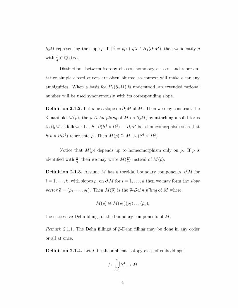
2.2 Left-handed Dehn twist about c. . . . . . . . . . . . . . . . . . 7
2.3 Twisting along an annulus R by surgery. . . . . . . . . . . . . 7
2.4 The correspondence of bases and framings. . . . . . . . . . . . 9
2.5 The once-punctured torus T . . . . . . . . . . . . . . . . . . . . 9
2.6 The diagram D . . . . . . . . . . . . . . . . . . . . . . . . . . 13
2.7 The edge-path E[2,−1]. . . . . . . . . . . . . . . . . . . . . . . 15
2.8 The subcomplex of D associated to a SCFE. . . . . . . . . . . 16
3.1 Left Handed Trefoil . . . . . . . . . . . . . . . . . . . . . . . . 27
3.2 Figure Eight Knot . . . . . . . . . . . . . . . . . . . . . . . . 27
3.3 The link L(5) and the Left Handed Trefoil. . . . . . . . . . . . 29
3.4 Minimally twisted 2n+ 1 chain. . . . . . . . . . . . . . . . . . 33
3.5 Twistings of 12ε for ε = ±1. . . . . . . . . . . . . . . . . . . . . 34
3.6 The link L(5, η) with an axis of strong involution and the genusone fibered knot. . . . . . . . . . . . . . . . . . . . . . . . . . 35
3.7 The quotient of the complement of the link L(5, η) by the stronginvolution, (B5, tL), followed by isotopies. . . . . . . . . . . . . 36
3.8 Further isotopies of (B5, tL). . . . . . . . . . . . . . . . . . . . 37
3.9 The tangles (B2n+1, tL) for each n even and odd. . . . . . . . . 38
3.10 The chain link C(5) with an axis of strong involution and thequotient of its complement, (B5, tC). . . . . . . . . . . . . . . 39
3.11 Isotopies of (B5, tC). . . . . . . . . . . . . . . . . . . . . . . . 40
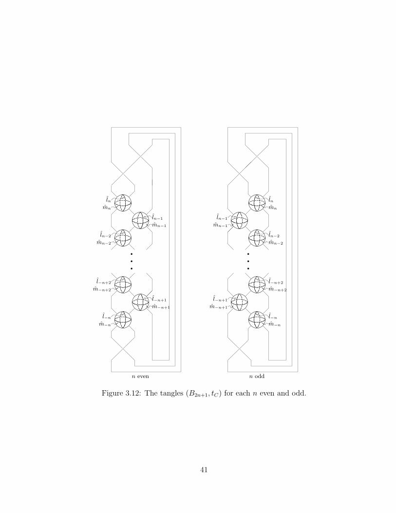
3.12 The tangles (B2n+1, tC) for each n even and odd. . . . . . . . . 41
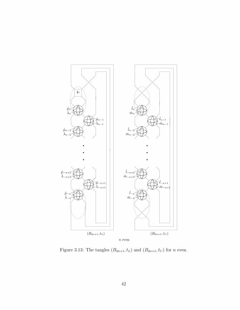
3.13 The tangles (B2n+1, tL) and (B2n+1, tC) for n even. . . . . . . . 42
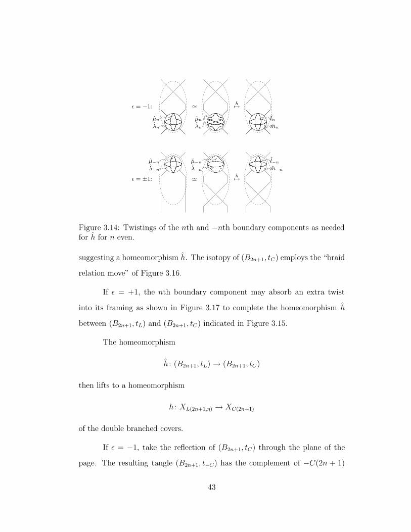
3.14 Twistings of the nth and −nth boundary components as neededfor h for n even. . . . . . . . . . . . . . . . . . . . . . . . . . . 43
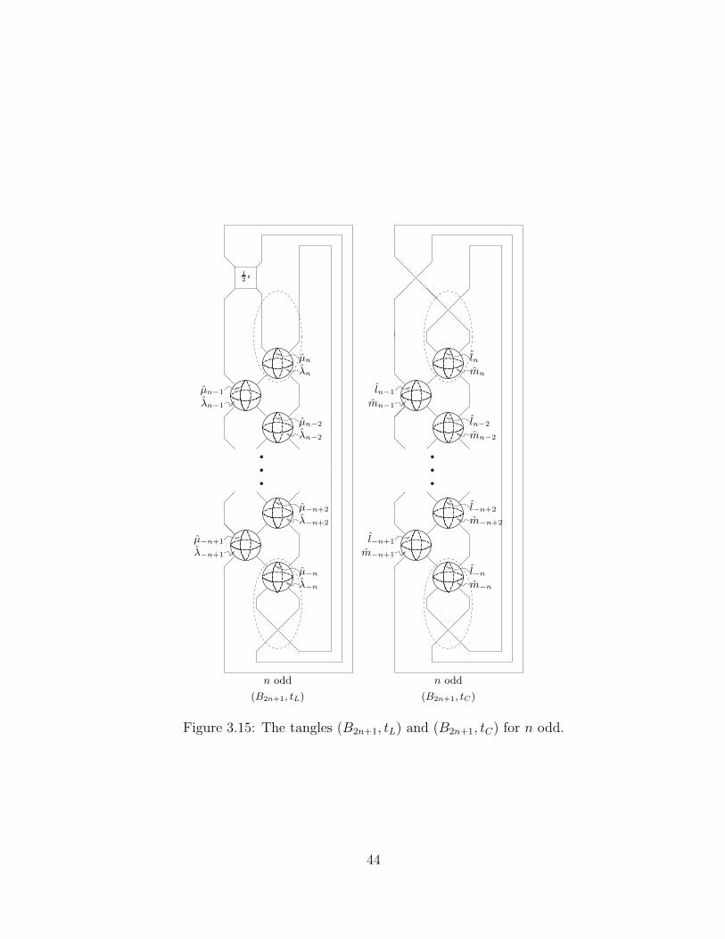
3.15 The tangles (B2n+1, tL) and (B2n+1, tC) for n odd. . . . . . . . 44
x
3.16 A braid isotopy. . . . . . . . . . . . . . . . . . . . . . . . . . . 45
3.17 Twisting of the nth boundary component as needed for h for nodd and ε = +1. . . . . . . . . . . . . . . . . . . . . . . . . . . 45
3.18 Twisting of the nth and −nth boundary components as neededfor h for n odd and ε = −1. . . . . . . . . . . . . . . . . . . . 46
4.1 The twisted saddle Ca,+2 with level knot a× ε. . . . . . . . 51
4.2 ‘Pushing’ α2 through Cb,+2 . . . . . . . . . . . . . . . . . . . . 52
4.3 The twisted saddles Ca,+2 and Cb,+2 joined in T × I/α2T × I . 53
4.4 Longitudinal annulus in C(0;n(k), . . . , n(2),±1). . . . . . . . . 84
4.5 Meridional annulus in C(0;n(k), . . . , n(2),±1). . . . . . . . . . 85
4.6 Boundary compressions of C(0;n(k), . . . , n(2),±1). . . . . . . 86
4.7 Adding sides to the first and last block. . . . . . . . . . . . . . 87
4.8 Adding sides to twisted saddles. . . . . . . . . . . . . . . . . . 87
A.1 Passing from a R-R diagrams to a surgery description. . . . . 114
A.2 Berge’s R-R diagram for type (I) knots (torus knots). . . . . . 114
A.3 Type (I) knots on Heegaard surface via surgeries. . . . . . . . 114
A.4 Type (I) knots. Isotopies and Kirby Calculus moves ending inthe MT5C. . . . . . . . . . . . . . . . . . . . . . . . . . . . . . 115
A.5 Berge’s R-R diagram for type (II) knots (cables about torusknots). . . . . . . . . . . . . . . . . . . . . . . . . . . . . . . . 116
A.6 Type (II) knots on Heegaard surface via surgeries. . . . . . . . 116
A.7 Type (II) knots. Isotopies and Kirby Calculus moves ending inthe MT5C. . . . . . . . . . . . . . . . . . . . . . . . . . . . . . 117
A.8 Berge’s R-R diagram for type (III) knots. . . . . . . . . . . . . 118
A.9 Type (III) knots on Heegaard surface via surgeries. . . . . . . 118
A.10 Type (III) knots. Isotopy to show parallel components. . . . . 119
A.11 Type (III) knots. Isotopies and Kirby Calculus moves endingin the MT5C. . . . . . . . . . . . . . . . . . . . . . . . . . . . 120
A.12 Berge’s R-R diagram for type (IV) knots. . . . . . . . . . . . . 121
A.13 Type (IV) knots on Heegaard surface via surgeries. . . . . . . 121
A.14 Type (IV) knots. Isotopies and Kirby Calculus moves. . . . . 122
A.15 Type (IV) knots. Isotopies and Kirby Calculus moves endingin the MT5C. . . . . . . . . . . . . . . . . . . . . . . . . . . . 123
xi

A.16 Berge’s R-R diagram for type (V) knots. . . . . . . . . . . . . 124
A.17 Type (V) knots on Heegaard surface via surgeries. . . . . . . . 124
A.18 Type (V) knots. Isotopies and Kirby Calculus moves. . . . . . 126
A.19 Type (V) knots. Isotopies and Kirby Calculus moves ending inthe MT5C. . . . . . . . . . . . . . . . . . . . . . . . . . . . . . 127
A.20 Berge’s R-R diagram for type (VI) knots. . . . . . . . . . . . . 128
A.21 Type (VI) knots on Heegaard surface via surgeries. . . . . . . 128
A.22 Type (VI) knots. Isotopies and Kirby Calculus moves. . . . . 130
A.23 Type (VI) knots. Isotopies and Kirby Calculus moves endingin the MT5C. . . . . . . . . . . . . . . . . . . . . . . . . . . . 131
A.24 Berge’s sporadic knot types a) and b) diagram. . . . . . . . . 132
A.25 Sporadic knot types a) and b) on Heegaard surface via surgeries.133
A.26 Sporadic types a) and b). One component bounds a Mobius band.133
A.27 Sporadic types a) and b). Core curve of Mobius band replacesthe boundary of Mobius band. . . . . . . . . . . . . . . . . . . 134
A.28 Sporadic types a) and b). Isotopies and Kirby Calculus movesending in the MT5C. . . . . . . . . . . . . . . . . . . . . . . . 135
A.29 Berge’s sporadic knot types c) and d) diagram. . . . . . . . . 136
A.30 Sporadic knot types c) and d) on Heegaard surface via surgeries. 137
A.31 Sporadic types c) and d). One component bounds a Mobius band.137
A.32 Sporadic types c) and d). Core curve of Mobius band replacesthe boundary of Mobius band. . . . . . . . . . . . . . . . . . . 138
A.33 Sporadic types c) and d). Isotopies and Kirby Calculus movesending in the MT5C. . . . . . . . . . . . . . . . . . . . . . . . 139
A.34 Berge knots Types I-VI . . . . . . . . . . . . . . . . . . . . . . 140
A.35 Sporadic Berge Knots . . . . . . . . . . . . . . . . . . . . . . . 141
B.1 Plumbing of Hopf bands . . . . . . . . . . . . . . . . . . . . . 143
B.2 Full positive twist . . . . . . . . . . . . . . . . . . . . . . . . . 143
B.3 The four train tracks. . . . . . . . . . . . . . . . . . . . . . . . 144
B.4 The four train tracks in braid position. . . . . . . . . . . . . . 145
B.5 Pre-split train tracks. . . . . . . . . . . . . . . . . . . . . . . . 146
B.6 Pre-split train tracks . . . . . . . . . . . . . . . . . . . . . . . 146
B.7 Moves for braiding train tracks on surfaces. . . . . . . . . . . . 147
xii
B.8 Sequence of moves for τ3 with the Left Handed Trefoil. . . . . 151
B.9 Sequence of moves for τ1 with the Figure Eight Knot. . . . . . 152
B.10 Sequence of moves for τ2 with the Figure Eight Knot. . . . . . 153
B.11 Summary of the braided train tracks. . . . . . . . . . . . . . . 154
xiii

Chapter 1
Introduction
As shown by Lickorish [14] and Wallace [21], any closed orientable 3-manifold
may be obtained by Dehn surgery on some link in S3. It is however not the
case that every such 3-manifold may be obtained by Dehn surgery on a knot.
One is prompted to then ask which 3-manifolds may be obtained by Dehn
surgery on a knot. Similarly one may ask to classify the knots with some
non-trivial Dehn surgery that yields a certain 3-manifold or a 3-manifold with
a certain property.
Perhaps the first two main questions along these lines are whether non-
trivial surgery on a knot in S3 can return S3 and more generally whether
non-trivial surgery on a knot in S3 can yield a simply connected manifold.
These are both very deep and difficult questions. The former was answered
in the negative by Gordon and Luecke [8]. The latter (known as Property P)
was more recently answered in the negative by Kronheimer, Mrowka, Ozsvath,
and Szabo [13].
The next “simplest” class of 3-manifolds are the lens spaces. They are
simple in the sense that they nearly simply connected having cyclic funda-
mental group and they have Heegaard genus 1. There are many examples of
1
knots with non-trivial surgeries yielding lens spaces. Berge [3] characterizes
all known examples of such knots and lists the knots with this characteriza-
tion. Conjecturally this list is complete. Though there has been much interest
recently in knots with lens space surgeries, this conjecture remains wide open.
We examine a certain family of these knots, the knots that lie as essen-
tial simple closed curves on the fiber of the Left Handed Trefoil, Right Handed
Trefoil, or Figure Eight Knot, and determine a marked difference between this
family of knots and the others that Berge describes. After reviewing defini-
tions and preliminary material in Chapter 2, we show in Chapter 3 that the
volumes of the hyperbolic knots in this family is unbounded. In Chapter 4
we develop a practical algorithm to list all the closed essential surfaces in the
complements of these knots. In Chapter 5 we tie the previous two chapters
together by finding relationships between volumes of the knots and the genera
of the closed essential surface (if any) contained in their complements. We
supplement this with two appendices. The first gives descriptions of the other
known knots with lens space surgeries as arising from surgeries on the Mini-
mally Twisted 5 Chain link. The second gives descriptions of the knots of our
primary interest as the closures of positive (or negative) braids.
2

Chapter 2
Definitions
Here we collect some of the basic definitions and concepts that we will use
throughout this paper. See any of the many knot theory and low dimensional
topology texts such as Rolfsen [17], Burde and Zieschang [5], or Kawauchi [11]
for a more thorough treatment of surgery, lens spaces, and fiber bundles. See
Thurston [20] or Benedetti and Petronio [2] for an introductions to hyperbolic
3-manifolds.
2.1 Surgery on Knots and Links
Let M be a compact, orientable 3-manifold with a toroidal boundary compo-
nent ∂0M .
Definition 2.1.1. A slope on ∂0M is an isotopy class of unoriented simple
closed curves.
Due to their lack of orientation, slopes are in a 2 to 1 correspondence
with primitive elements of π1(∂0M) ∼= H1(∂0M ; Z) ∼= Z2. Given a choice of
basis for H1(∂0M), say µ, λ, we may identify the set of slopes on ∂0M with
the extended rationals Q ∪ ∞: Let c be an oriented simple closed curve on
3
∂0M representing the slope ρ. If [c] = pµ+ qλ ∈ H1(∂0M), then we identify ρ
with p
q∈ Q ∪∞.
Distinctions between isotopy classes, homology classes, and represen-
tative simple closed curves are often blurred as context will make clear any
ambiguities. When a basis for H1(∂0M) is understood, an extended rational
number will be used synonymously with its corresponding slope.
Definition 2.1.2. Let ρ be a slope on ∂0M of M . Then we may construct the
3-manifold M(ρ), the ρ-Dehn filling of M on ∂0M , by attaching a solid torus
to ∂0M as follows. Let h : ∂(S1 ×D2) → ∂0M be a homeomorphism such that
h(∗ × ∂D2) represents ρ. Then M(ρ) ∼= M ∪h (S1 ×D2).
Notice that M(ρ) depends up to homeomorphism only on ρ. If ρ is
identified with p
q, then we may write M(p
q) instead of M(ρ).
Definition 2.1.3. Assume M has k toroidal boundary components, ∂iM for
i = 1, . . . , k, with slopes ρi on ∂iM for i = 1, . . . , k then we may form the slope
vector ρ = (ρ1, . . . , ρk). Then M(ρ) is the ρ-Dehn filling of M where
M(ρ) ∼= M(ρ1)(ρ2) . . . (ρk),
the successive Dehn fillings of the boundary components of M .
Remark 2.1.1. The Dehn fillings of ρ-Dehn filling may be done in any order
or all at once.
Definition 2.1.4. Let L be the ambient isotopy class of embeddings
f :
k⋃
i=1
S1i →M
4

of k circles so that f(S1i ) has a regular neighborhood for each i. Then L is a
k component (tame) link in M . If L has only one component, then we say L
is a knot in M .
Definition 2.1.5. Let L be a link in S3. Let N(L) be a regular open neigh-
borhood of L. Then the exterior of L is the manifold XL = S3 −N(L).
Remark 2.1.2. If L is a k component link, then ∂XL is a disjoint union of k
tori.
Definition 2.1.6. Let L be a k component link in S3. Let ∂XL =⋃k
i=1 ∂iXL,
and let ρ be a slope vector of slopes ρi on ∂iXL. We say the manifold XL(ρ)
is obtained by ρ-Dehn surgery on L.
Let Li be the ith component of a link L in S3 with some chosen orien-
tation. Given a non-trivial simple closed curve mi on ∂N(Li) that bounds a
disk in N(Li), orient mi so that the linking number of mi and Li is +1. For
a simple closed curve li on ∂N(Li) parallel to Li in N(Li), orient li coher-
ently with Li. Note that these orientations (with the orientation on ∂N(Li)
induced by the orientation on N(Li)) imply the algebraic intersection number
mi · li = +1. See Figure 2.1 for a depiction of Li, mi, and li.
Li
li
mi
Figure 2.1: A meridian and longitude for Li.
5

Definition 2.1.7. We say that mi is a meridian of Li and that li is a longitude.
If li is the boundary of an orientable surface in X(Li) (a Seifert surface), then
we say the pair mi, li is a standard meridian-longitude pair. We use these
terms for the corresponding unoriented curves, elements of H1(∂N(Li)), and
slopes as well. For µi = [mi], λi = [li] ∈ H1(∂N(Li)), we say µi, λi is the
standard basis for H1(∂N(Li)).
Remark 2.1.3. Notice that choosing the opposite orientation of Li changes the
orientation of the meridian and hence the longitude too. This change however
has no net effect on a slope p
q.
More generally:
Definition 2.1.8. A pair of (oriented) simple closed curves m and l on a torus
T such that m · l = +1 form a basis for T , and their homology classes [m] and
[l] ∈ H1(T ) form a basis for H1(T ).
2.1.1 Dehn Twists
Let c be a simple closed curve on the orientable surface S.
Definition 2.1.9. The homeomorphism S → S defined by cutting S along c
and regluing along c after rotating a full counter-clockwise turn is called the
left-handed Dehn twist of S about c.
See Figure 2.2 for a sketch of the effect of this homeomorphism. Note
that this homeomorphism is isotopic to the identity outside a neighborhood of
c.
6
c7→
c
Figure 2.2: Left-handed Dehn twist about c.
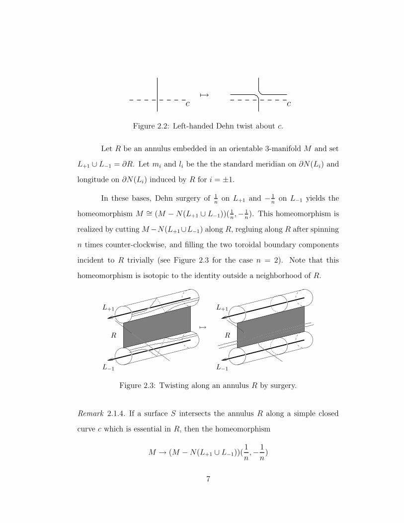
Let R be an annulus embedded in an orientable 3-manifold M and set
L+1 ∪ L−1 = ∂R. Let mi and li be the the standard meridian on ∂N(Li) and
longitude on ∂N(Li) induced by R for i = ±1.
In these bases, Dehn surgery of 1n
on L+1 and − 1n
on L−1 yields the
homeomorphism M ∼= (M − N(L+1 ∪ L−1))(1n,− 1
n). This homeomorphism is
realized by cutting M−N(L+1∪L−1) along R, regluing along R after spinning
n times counter-clockwise, and filling the two toroidal boundary components
incident to R trivially (see Figure 2.3 for the case n = 2). Note that this
homeomorphism is isotopic to the identity outside a neighborhood of R.
R
L−1
L+1
R
L−1
L+1
7→
Figure 2.3: Twisting along an annulus R by surgery.
Remark 2.1.4. If a surface S intersects the annulus R along a simple closed
curve c which is essential in R, then the homeomorphism
M → (M −N(L+1 ∪ L−1))(1
n,−
1
n)
7

restricted to S is the composition of n left-handed Dehn twists.
2.1.2 Tangles
Definition 2.1.10. A tangle (B, t) is a pair consisting of a punctured 3-sphere
B and a properly embedded collection t of disjoint arcs and simple closed
curves. Two tangles (B1, t1) and (B2, t2) are homeomorphic if there is a home-
omorphism of pairs
h : (B1, t1) → (B2, t2).
A boundary component (∂B0, t∩∂B0) of a tangle (B, t) is a sphere ∂B0
together with some finite number of points t ∩ ∂B0.
Definition 2.1.11. Given a sphere S and set p of four distinct points on S, a
framing of (S, p) is an ordered pair of (unoriented) simple closed curves (m, l)
on S −N(p) such that each curve separates different pairs of points of p.
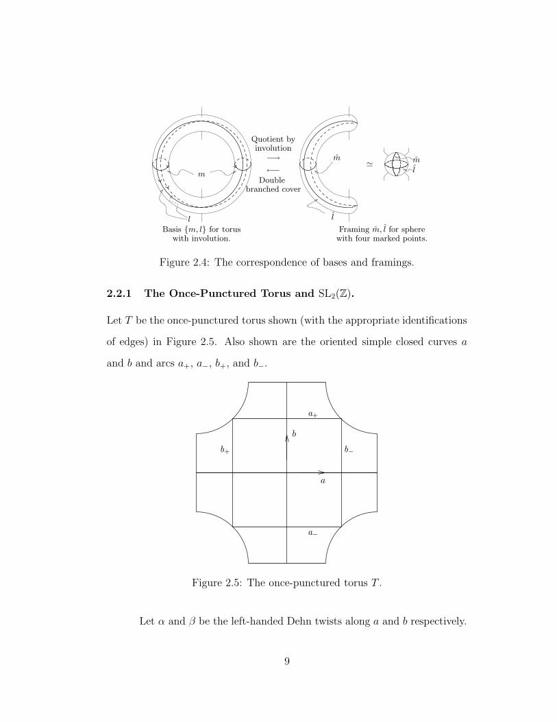
Let (S, p) be a sphere with four points with framing (m, l). The double
cover of S branched over p is a torus. Single components, say m and l, of the
lifts of the framing curves m and l when oriented so that m · l = +1 (with
respect to the orientation of the torus) form a basis for the torus. Similarly, a
basis on a torus induces a framing on the sphere with four points obtained by
the quotient of an involution that fixes four points on the torus. See Figure
2.4.
2.2 Surfaces and Bundles
The notation and terminology we set up in §§2.2.1 and 2.2.2 is borrowed from
Culler, Jaco, and Rubinstein [6] so that our work will be consistent with theirs.
8
m
l
Basis m, l for toruswith involution.
m
l
m
l
Framing m, l for spherewith four marked points.
'
Quotient byinvolution
Doublebranched cover
−→
←−
Figure 2.4: The correspondence of bases and framings.
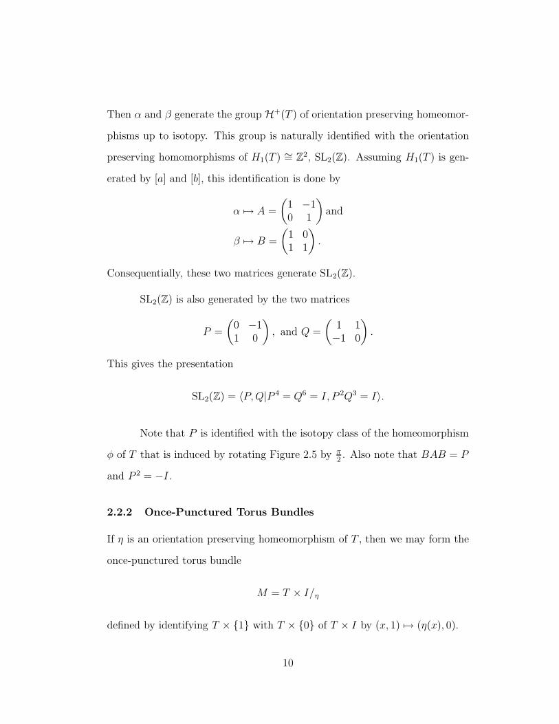
2.2.1 The Once-Punctured Torus and SL2(Z).
Let T be the once-punctured torus shown (with the appropriate identifications
of edges) in Figure 2.5. Also shown are the oriented simple closed curves a
and b and arcs a+, a−, b+, and b−.
b
a
a+
a−
b−b+
Figure 2.5: The once-punctured torus T .
Let α and β be the left-handed Dehn twists along a and b respectively.
9
Then α and β generate the group H+(T ) of orientation preserving homeomor-
phisms up to isotopy. This group is naturally identified with the orientation
preserving homomorphisms of H1(T ) ∼= Z2, SL2(Z). Assuming H1(T ) is gen-
erated by [a] and [b], this identification is done by
α 7→ A =
(1 −10 1
)and
β 7→ B =
(1 01 1
).
Consequentially, these two matrices generate SL2(Z).
SL2(Z) is also generated by the two matrices
P =
(0 −11 0
), and Q =
(1 1−1 0
).
This gives the presentation
SL2(Z) = 〈P,Q|P 4 = Q6 = I, P 2Q3 = I〉.
Note that P is identified with the isotopy class of the homeomorphism
φ of T that is induced by rotating Figure 2.5 by π2. Also note that BAB = P
and P 2 = −I.
2.2.2 Once-Punctured Torus Bundles
If η is an orientation preserving homeomorphism of T , then we may form the
once-punctured torus bundle
M = T × I/η
defined by identifying T × 1 with T × 0 of T × I by (x, 1) 7→ (η(x), 0).
10

If we express η as a composition of such homeomorphisms
η = ηnηn−1 . . . η2η1, then M may be divided into “blocks” as
M = T × I/η1T × I/η2 . . . /ηn−1T × I/ηn
where T ×1 of the ith block is identified with T ×0 of the i+1th (mod n)
block according to (x, 1)i 7→ (ηi(x), 0)i+1.
If Hi is identified with the isotopy class of the homeomorphism ηi, then
M has characteristic class [HnHn−1 . . .H2H1].
2.2.3 Essential Curves and Surfaces
Definition 2.2.1. Let c be a simple closed curve on a compact orientable
surface S. If c does not bound a disk in S and does not bound an annulus
with a component of ∂S, then c is an essential curve.
Definition 2.2.2. Let S be a properly embedded compact orientable surface
in a compact orientable 3-manifold. If S is incompressible, ∂-incompressible,
and not ∂-parallel, then S is an essential surface.
Definition 2.2.3. If M is a compact orientable 3-manifold that contains no
essential closed orientable surfaces, then M is small.
11
2.3 Continued Fractions
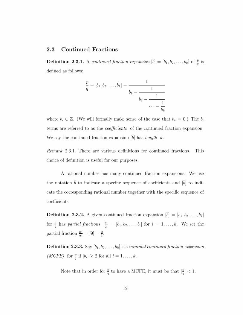
Definition 2.3.1. A continued fraction expansion [b] = [b1, b2, . . . , bk] of p
qis
defined as follows:
p
q= [b1, b2, . . . , bk] =
1
b1 −1
b2 −1
· · · −1
bk
where bi ∈ Z. (We will formally make sense of the case that bk = 0.) The bi
terms are referred to as the coefficients of the continued fraction expansion.
We say the continued fraction expansion [b] has length k.
Remark 2.3.1. There are various definitions for continued fractions. This
choice of definition is useful for our purposes.
A rational number has many continued fraction expansions. We use
the notation b to indicate a specific sequence of coefficients and [b] to indi-
cate the corresponding rational number together with the specific sequence of
coefficients.
Definition 2.3.2. A given continued fraction expansion [b] = [b1, b2, . . . , bk]
for p
qhas partial fractions pi
qi= [b1, b2, . . . , bi] for i = 1, . . . , k. We set the
partial fraction p0q0
= [∅] = 01.
Definition 2.3.3. Say [b1, b2, . . . , bk] is a minimal continued fraction expansion
(MCFE) for p
qif |bi| ≥ 2 for all i = 1, . . . , k.
Note that in order for p
qto have a MCFE, it must be that | p
q| < 1.
12

Definition 2.3.4. Say [b1, b2, . . . , bk] is the simple continued fraction expansion
(SCFE) for p
qif the coefficients alternate signs, |bk| ≥ 2, and bi 6= 0 for i ≥ 2.
Notice that though continued fraction expansions are not unique, each
rational number p
qdoes have a unique SCFE. Furthermore, the SCFE for p
q
has 0 as its first coefficient if and only if | pq| ≥ 1 (see Lemma 2.3.1).
Definition 2.3.5. Let D be the diagram shown in Figure 2.6. D is a disk
with the extended rational numbers marked on its boundary. An edge joins
vertices ab
to cd
if and only if ad− bc = ±1. The edge from ab
to cd
is the ’long’
edge of the triangle whose third vertex is a+cb+d
.
− 23
01
13
12
23
11
32
21
31
10
− 12
− 13
− 31
− 21
− 32
− 11
Figure 2.6: The diagram D
Remark 2.3.2. D is in fact the classical diagram of the action of the modular
group PSL2(Z) on the hyperbolic plane H2 viewed as the Poincare disk. We
13
utilize the connections between D, SL2(Z) (and PSL2(Z)), and continued frac-
tion expansions in the vein of Floyd-Hatcher [7] and Hatcher-Thurston [10]
and borrow some of their terminology. One may look to Kirby-Melvin [12] for
a more thorough treatment of these connections.
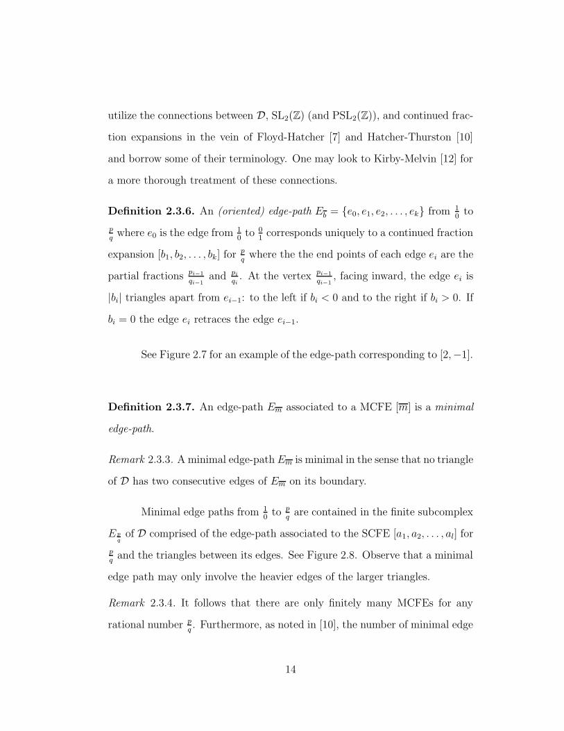
Definition 2.3.6. An (oriented) edge-path Eb = e0, e1, e2, . . . , ek from 10
to
p
qwhere e0 is the edge from 1
0to 0
1corresponds uniquely to a continued fraction
expansion [b1, b2, . . . , bk] for p
qwhere the the end points of each edge ei are the
partial fractions pi−1
qi−1and pi
qi. At the vertex pi−1
qi−1, facing inward, the edge ei is
|bi| triangles apart from ei−1: to the left if bi < 0 and to the right if bi > 0. If
bi = 0 the edge ei retraces the edge ei−1.
See Figure 2.7 for an example of the edge-path corresponding to [2,−1].
Definition 2.3.7. An edge-path Em associated to a MCFE [m] is a minimal
edge-path.
Remark 2.3.3. A minimal edge-path Em is minimal in the sense that no triangle
of D has two consecutive edges of Em on its boundary.
Minimal edge paths from 10
to p
qare contained in the finite subcomplex
E p
qof D comprised of the edge-path associated to the SCFE [a1, a2, . . . , al] for
p
qand the triangles between its edges. See Figure 2.8. Observe that a minimal
edge path may only involve the heavier edges of the larger triangles.
Remark 2.3.4. It follows that there are only finitely many MCFEs for any
rational number p
q. Furthermore, as noted in [10], the number of minimal edge
14
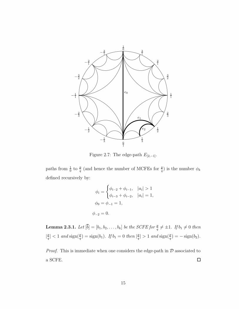
e0
e1
e2
− 23
01
13
12
23
11
32
21
31
10
− 12
− 13
− 31
− 21
− 32
− 11
Figure 2.7: The edge-path E[2,−1].
paths from 10
to p
q(and hence the number of MCFEs for p
q) is the number φk
defined recursively by:
φi =
φi−2 + φi−1, |ai| > 1
φi−3 + φi−2, |ai| = 1,
φ0 = φ−1 = 1,
φ−2 = 0.
Lemma 2.3.1. Let [b] = [b1, b2, . . . , bk] be the SCFE for p
q6= ±1. If b1 6= 0 then
|pq| < 1 and sign(p
q) = sign(b1). If b1 = 0 then |p
q| > 1 and sign(p
q) = − sign(b2).
Proof. This is immediate when one considers the edge-path in D associated to
a SCFE.
15
1/0 [b1] [b1, b2, b3]
or[b1, b2, . . . , bk−1]
[b1, b2, . . . , bk−1]
[b1, b2, . . . , bk]
[b1, b2, . . . , bk]
[b1, b2]0/1
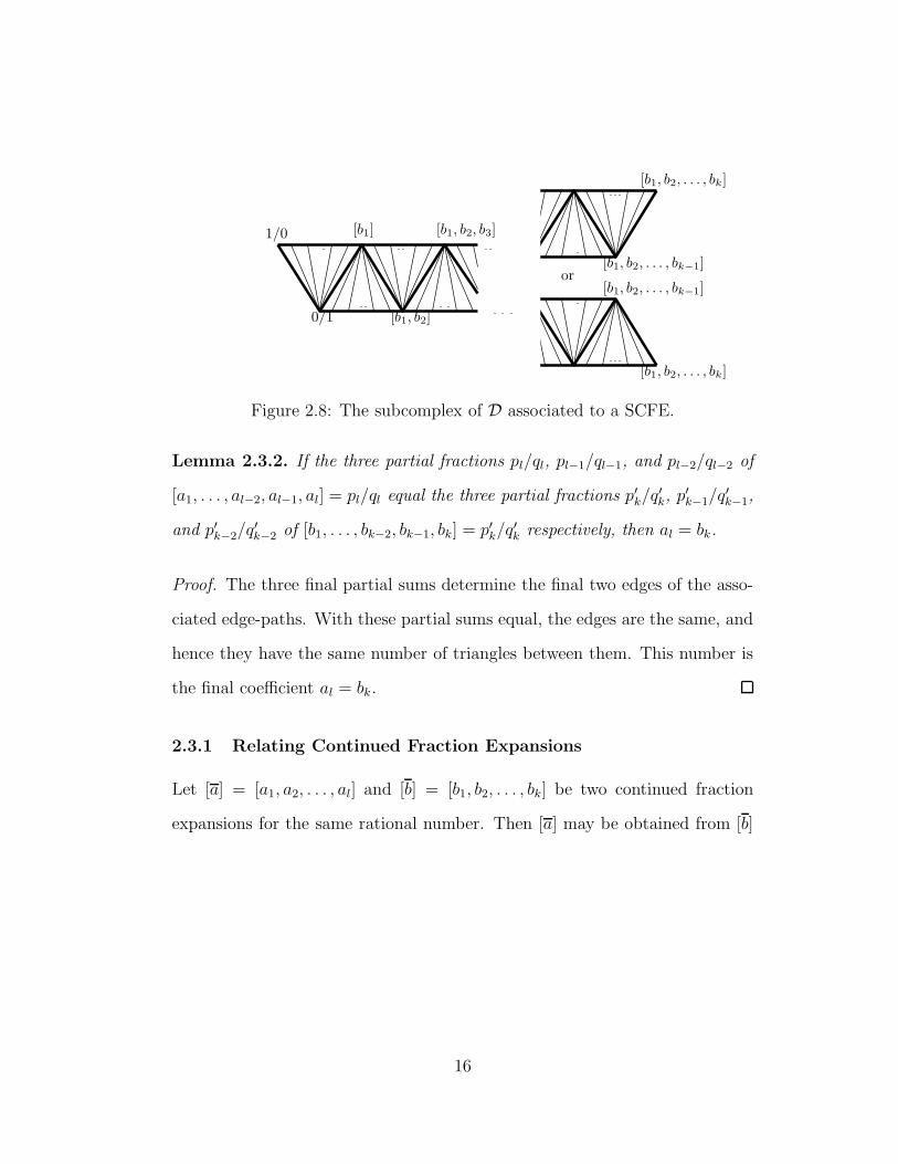
Figure 2.8: The subcomplex of D associated to a SCFE.
Lemma 2.3.2. If the three partial fractions pl/ql, pl−1/ql−1, and pl−2/ql−2 of
[a1, . . . , al−2, al−1, al] = pl/ql equal the three partial fractions p′k/q′k, p
′k−1/q
′k−1,
and p′k−2/q′k−2 of [b1, . . . , bk−2, bk−1, bk] = p′k/q
′k respectively, then al = bk.
Proof. The three final partial sums determine the final two edges of the asso-
ciated edge-paths. With these partial sums equal, the edges are the same, and
hence they have the same number of triangles between them. This number is
the final coefficient al = bk.
2.3.1 Relating Continued Fraction Expansions
Let [a] = [a1, a2, . . . , al] and [b] = [b1, b2, . . . , bk] be two continued fraction
expansions for the same rational number. Then [a] may be obtained from [b]
16
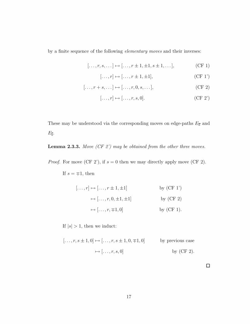
by a finite sequence of the following elementary moves and their inverses:
[. . . , r, s, . . . ] 7→ [. . . , r ± 1,±1, s± 1, . . . ], (CF 1)
[. . . , r] 7→ [. . . , r ± 1,±1], (CF 1’)
[. . . , r + s, . . . ] 7→ [. . . , r, 0, s, . . . ], (CF 2)
[. . . , r] 7→ [. . . , r, s, 0]. (CF 2’)
These may be understood via the corresponding moves on edge-paths Ea and
Eb.
Lemma 2.3.3. Move (CF 2’) may be obtained from the other three moves.
Proof. For move (CF 2’), if s = 0 then we may directly apply move (CF 2).
If s = ∓1, then
[. . . , r] 7→ [. . . , r ± 1,±1] by (CF 1’)
7→ [. . . , r, 0,±1,±1] by (CF 2)
7→ [. . . , r,∓1, 0] by (CF 1).
If |s| > 1, then we induct:
[. . . , r, s± 1, 0] 7→ [. . . , r, s± 1, 0,∓1, 0] by previous case
7→ [. . . , r, s, 0] by (CF 2).
17
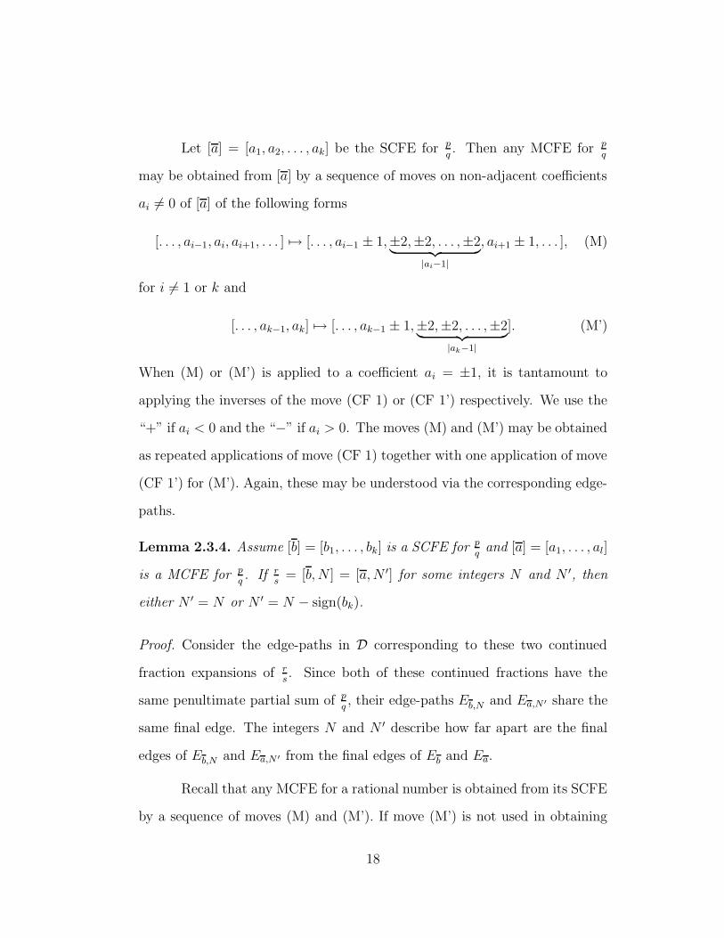
Let [a] = [a1, a2, . . . , ak] be the SCFE for p
q. Then any MCFE for p
q
may be obtained from [a] by a sequence of moves on non-adjacent coefficients
ai 6= 0 of [a] of the following forms
[. . . , ai−1, ai, ai+1, . . . ] 7→ [. . . , ai−1 ± 1,±2,±2, . . . ,±2︸ ︷︷ ︸|ai−1|
, ai+1 ± 1, . . . ], (M)
for i 6= 1 or k and
[. . . , ak−1, ak] 7→ [. . . , ak−1 ± 1,±2,±2, . . . ,±2︸ ︷︷ ︸|ak−1|
]. (M’)
When (M) or (M’) is applied to a coefficient ai = ±1, it is tantamount to
applying the inverses of the move (CF 1) or (CF 1’) respectively. We use the
“+” if ai < 0 and the “−” if ai > 0. The moves (M) and (M’) may be obtained
as repeated applications of move (CF 1) together with one application of move
(CF 1’) for (M’). Again, these may be understood via the corresponding edge-
paths.
Lemma 2.3.4. Assume [b] = [b1, . . . , bk] is a SCFE for p
qand [a] = [a1, . . . , al]
is a MCFE for p
q. If r
s= [b, N ] = [a,N ′] for some integers N and N ′, then
either N ′ = N or N ′ = N − sign(bk).
Proof. Consider the edge-paths in D corresponding to these two continued
fraction expansions of rs. Since both of these continued fractions have the
same penultimate partial sum of p
q, their edge-paths Eb,N and Ea,N ′ share the
same final edge. The integers N and N ′ describe how far apart are the final
edges of Eb,N and Ea,N ′ from the final edges of Eb and Ea.
Recall that any MCFE for a rational number is obtained from its SCFE
by a sequence of moves (M) and (M’). If move (M’) is not used in obtaining
18

[a] from [b] then Ea and Eb have the same final edge. In this case, N ′ = N .
This case may also be viewed as a consequence of Lemma 2.3.2.
If move (M’) is used in obtaining [a] from [b] then the final edges of Ea
and Eb are distinct edges of a triangle ∆ in D sharing the vertex at p
q. The
final edge of Eb is bk triangles (counted with sign) apart from the penultimate
edge of Eb. These bk triangles cross third edge of ∆, and hence the final edge
of Eb is sign(bk) triangles apart from the third edge of ∆. Therefore the final
edge of Eb is − sign(bk) triangles apart from the final edge of Ea. This implies
that the final edge of Eb,N is N + − sign(bk) edges apart from the final edge
of Ea. Thus the final edge of Ea,N ′ is N − sign(bk) edges apart from the final
edge of Ea so that N ′ = N − sign(bk).
Coefficient Sums.
Definition 2.3.8. If [b] = [b1, b2, . . . , bk] is a continued fraction expansion,
then σ(b) =∑k
i=1 bi is the coefficient sum of [b].
Assume [b′] is obtained from [b] by an elementary move. Then the
coefficient sums differ as follows:
σ(b′) − σ(b) =
±3 if [b′] is obtained by (CF 1),
±2 if [b′] is obtained by (CF 1’),
0 if [b′] is obtained by (CF 2).
The difference varies, however, if [b′] is obtained from [b] by move (CF 2’).
Also if [b′] is obtained from [b] by move (M) at bi for 1 < i < k or move (M’)
at bk, then
σ(b′) − σ(b) =
−3bi if i 6= k,
−3bk + 1 if bk > 0,
−3bk − 1 if bk < 0.
19

Lengths.
Assume [b′] is obtained from [b] by an elementary move. Then the lengths
differ as follows:
length(b′) − length(b) =
1 if [b′] is obtained by (CF 1) or (CF 1’),
2 if [b′] is obtained by (CF 2) or (CF 2’).
Also if [b′] is obtained from [b] by move (M) or (M’) at bi then
length(b′) − length(b) = |bi| − 2.
2.3.2 SL2(Z) and Continued Fraction Expansions
Lemma 2.3.5. Let W =
(x ty u
)∈ SL2(Z). Then
1. depending on the parity of k
W = ±Bn1An2 . . . Bnk or ±BABAn1Bn2 . . . Bnk
if and only ifxy
= [n1, n2, . . . , nk] and tu
= [n1, n2, . . . , nk−1],
and
2. depending on the parity of k
W = ±Bn1An2 . . . Ank or ±BABAn1Bn2 . . . Ank
if and only ifxy
= [n1, n2, . . . , nk−1] and tu
= [n1, n2, . . . , nk].
Proof. Note that if rs
= [n1, n2, . . . , nk] then rs
= [1, 1, 1, n1, n2, . . . , nk] by
moves (CF 1) and (CF 2). Thus we may assume k is odd or even as needed.
Case 1. We proceed by induction on odd integers.
If k = 1, then we are done as W = Bn1 =
(1 0n1 1
)and 1
n1= [n1] and
01
= [∅].
20

Assume W = ±Bn3 . . . Ank−1Bnk =
(x ty u
)where x
y= [n3, . . . , nk−1, nk]
and tu
= [n3, . . . , nk−1]. Consider
Bn1An2 =
(1 −n2
n1 1 − n1n2
).
Then
Bn1An2W =
(1 −n2
n1 1 − n1n2
)(x ty u
)
=
(x− n2y t− n2y
n1x+ y − n1n2y n1t + u− n1n2u
).
Thus
x− n2y
n1x+ y − n1n2y=
1n1(x−n2y)−−y
x−n2y
=1
n1 −−y
x−n2y
=1
n1 −1
n2y−xy
=1
n1 −1
n2 −xy
=1
n1 −1
n2 − [n3, . . . , nk]
= [n1, n2, n3, . . . , nk].
Similarly t−n2un1t+u−n1n2u
= [n1, n2, n3, . . . , nk−1].
Case 2. Since [n1] = [1, 1, 1, n1], we proceed by induction on even
integers.
If k = 2 then W = Bn1An2 =
(1 −n2
n1 1 − n1n2
). We are then done since
−n2
1 − n1n2
=1
n1 −1
n2
= [n1, n2],
and 1/n1 = [n1].
21

When k > 2, the conclusion follows as in case 1.
The lemma then follows.
Lemma 2.3.6. Let W =
(x ty u
)∈ SL2(Z) and x
y= [n1, n2, . . . , nk]. Then
depending on the parity of k,
W = ±Bn1An2 . . . BnkANor ±BABAn1Bn2 . . . BnkAN
for some N ∈ Z.
Proof. Let W0 =
(x t0y u0
)where t0
u0is in lowest terms with continued fraction
expansion [n1, n2, . . . , nk−1]. Then since W0 ∈ SL2(Z),
W−10 W =
(u0 −t0−y x
)(x ty u
)
=
(1 tu0 − ut00 1
)= Aut0−tu0 .
Thus W = W0AN where N = ut0 − tu0. Then by applying Lemma 2.3.5 to
W0 we are done.
Definition 2.3.9. Assume W ∈ SL2(Z) may be expressed as
W = P JCnk . . . Bn2An1
where |ni| ≥ 2 for i = 2, . . . , k such that if k is odd J ∈ 0, 2 and C = B,
and if k is even J ∈ −1,+1 and C = A. We call such an expression for W
a special form.
Remark 2.3.5. Contrast this with the special form of [6].
22
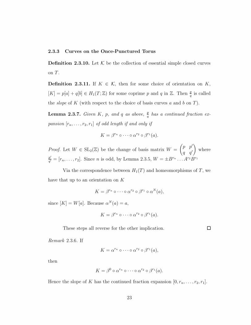
2.3.3 Curves on the Once-Punctured Torus
Definition 2.3.10. Let K be the collection of essential simple closed curves
on T .
Definition 2.3.11. If K ∈ K, then for some choice of orientation on K,
[K] = p[a] + q[b] ∈ H1(T ; Z) for some coprime p and q in Z. Then p
qis called
the slope of K (with respect to the choice of basis curves a and b on T ).
Lemma 2.3.7. Given K, p, and q as above, p
qhas a continued fraction ex-
pansion [rn, . . . , r2, r1] of odd length if and only if
K = βrn · · · αr2 βr1(a).
Proof. Let W ∈ SL2(Z) be the change of basis matrix W =
(p p′
q q′
)where
p′
q′= [rn, . . . , r2]. Since n is odd, by Lemma 2.3.5, W = ±Brn . . . Ar2Br1
Via the correspondence between H1(T ) and homeomorphisms of T , we
have that up to an orientation on K
K = βrn · · · αr2 βr1 αN(a),
since [K] = W [a]. Because αN(a) = a,
K = βrn · · · αr2 βr1(a).
These steps all reverse for the other implication.
Remark 2.3.6. If
K = αrn · · · αr2 βr1(a),
then
K = β0 αrn · · · αr2 βr1(a).
Hence the slope of K has the continued fraction expansion [0, rn, . . . , r2, r1].
23
2.4 Lens Spaces and Berge Knots
2.4.1 Lens Spaces
Consider the unknot in S3, and let p
qbe a slope in the standard basis.
Definition 2.4.1. A lens space is the 3-manifold L(p, q) ∼= XUnknot(p
q).
Notice that a lens space is the union of two solid tori identified along
their boundaries. Typically we exclude the special cases S3 ∼= L(1, n) for n ∈ Z
and S1 × S2 ∼= L(0, 1) from being called lens spaces.
Definition 2.4.2. If K is a knot in S3, then we say K admits a lens space
surgery if XK(pq) is a lens space for some slope p
q.
2.4.2 Berge Knots
See Berge’s paper [3] for a complete description of this collection of knots.
Let H1 be a standardly embedded genus 2 handlebody in S3, and let
H2 be its complementary (genus 2) handlebody. Set Σ = ∂H1 = ∂H2, and let
K be a simple closed curve on Σ.
Definition 2.4.3. If K represents a primitive element of π1(Hi) ∼= Z ∗ Z for
both i = 1, 2, then we say K is a double primitive curve on Σ.
Recall that if a is a primitive element of the group Z ∗ Z, then there
exists an element b ∈ Z ∗ Z such that 〈a, b〉 ∼= Z ∗ Z. The condition that K
represents a primitive element in π1(Hi) is equivalent to the existence of a
properly embedded disk Di in Hi so that |K ∩ ∂Di| = 1, i = 1, 2.
Theorem 2.4.1. (Berge [3]) If K is a double primitive curve on Σ, then K
admits a lens space surgery.
24
Definition 2.4.4. The knots that may be written as double primitive curves
on Σ are referred to as Berge knots.
2.4.3 Knots on a Genus One Fiber
Definition 2.4.5. Let Kη be the image of K under the inclusion
T → T × 0 ⊂ T × I/η = Mη.
If K ∈ Kη is a knot in the once-punctured torus bundle Mη, then we say that
K is a level knot .
Note that a level knot K ⊂ Mη is “level” in the sense that K is con-
tained in a level set of the projection p : Mη → S1 where each fiber is the
preimage of a point.
When T × I/η ⊂ S3 is a knot complement (i.e. the complement of a
trefoil or the Figure Eight Knot), we also let Kη be the image of K under the
further inclusion T → T × 0 ⊂ T × I/η ⊂ S3. In these cases, Kη is the
family of knots on the fiber of a trefoil or the Figure Eight Knot. These two
families are Berge’s families VII) and VIII) in [3] respectively. Thus the knots
in Kη are Berge knots and hence have lens space surgeries. These knots are
the primary focus of this dissertation.
Remark 2.4.1. Berge describes his knots up to reflection. The knots in Berge’s
family VII) are those that lie on the fiber of the Right Handed Trefoil. We
however typically work with the family of knots that lie on the fiber of the Left
Handed Trefoil and obtain the family of knots that lie on the Right Handed
Trefoil by reflection. When setup as in the beginning of the following chapter,
25
our knots of slope xy
on the fiber of the Left Handed Trefoil correspond by
reflection to Berge’s knots [k] = −x[g1] + y[g2] of his family VII). Note this
difference when using Berge’s calculation of the lens spaces yielded by surgery
on these knots.
26
Chapter 3
Surgery Descriptions of Knots
3.1 Surgery Description of Knots on a Genus One Fiber
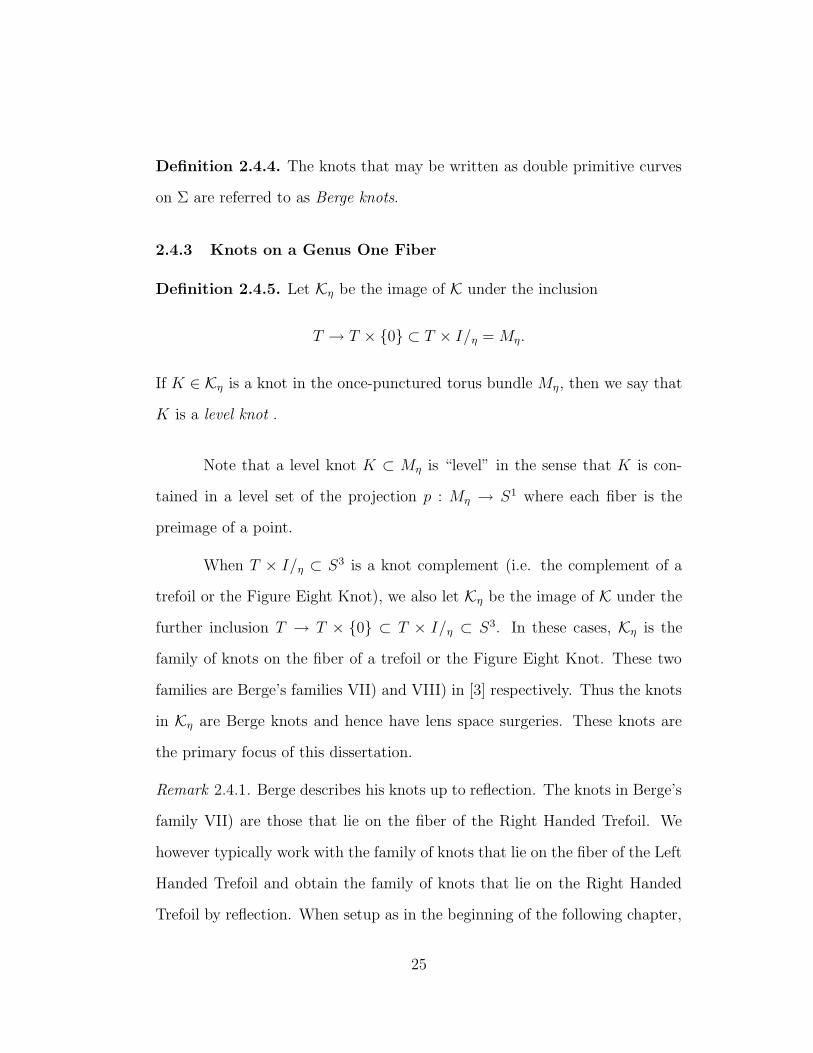
Recall (§2.2.1) T is a once-punctured torus and a and b are oriented simple
closed curves on T that intersect once as in Figure 2.5. Assume T is oriented
so that a · b = +1.
b a
Figure 3.1: Left Handed Trefoil with fiber and basis.
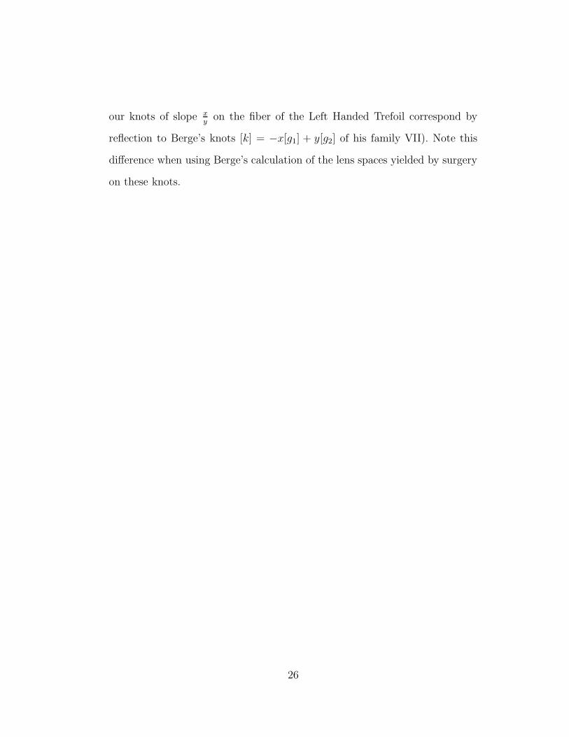
b a
Figure 3.2: Figure Eight Knot with fiber and basis.
27

Also recall the construction in §2.2.2 of a once-punctured torus bundle
T×I/η where I = [0, 1] and (x, 1) ∼ (η(x), 0). Equivalently, (η−1(x), 1) ∼ (x, 0).
In this chapter let us view once-punctured torus bundles slightly differently.
LetMη denote the fiber bundle T×[−n, n+1]/η where (η−1(x), n + 1) ∼ (x,−n)
for some n ∈ N and some homeomorphism η : T → T . If η−1 = β α, then
Mη may be recognized as the complement of the Left Handed Trefoil depicted
in Figure 3.1 (as the boundary of the plumbing of two negative Hopf bands).
If η−1 = α−1 β−1, then Mη is the complement of the Right Handed
Trefoil. The Right Handed Trefoil may be obtained from the Left Handed
Trefoil by reflecting Figure 3.1 through the plane of the page. Consequentially,
the complement of the Right Handed Trefoil is that of the Left Handed Trefoil
with opposite orientation. For this reason we will not be expressly dealing
with the Right Handed Trefoil.
If η−1 = β α−1, then Mη is the complement of the Figure Eight Knot
depicted in Figure 3.2 (as the boundary of the plumbing of a positive Hopf
band onto a negative Hopf band). Note that in all cases, Mη ⊂ S3.
Throughout the remainder of this chapter, η−1 is assumed to be either
β α or β α−1.
3.1.1 The link L(2n + 1, η).
Consider Mη = T×[−n, n+1]/η ⊂ S3. For n ∈ N and i ∈ −n,−n+1, . . . , n,
set Li = a× i or Li = b× i if i is even or odd respectively.
28
L−1
L1
L−2
L0
L2
Left Handed Trefoil
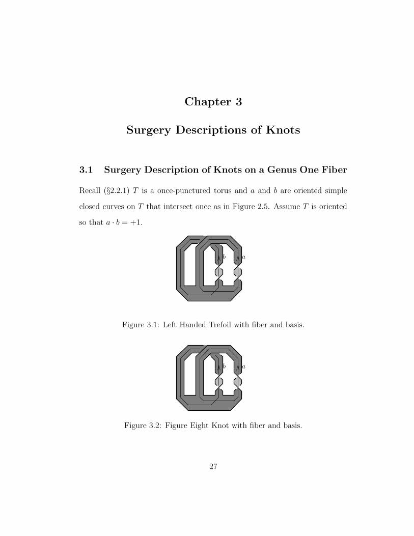
Figure 3.3: The link L(5) and the Left Handed Trefoil.
Definition 3.1.1. Define L(2n + 1, η) to be the oriented link
n⋃
i=−n
Li ⊂ Mη ⊂ S3.
We write L(2n + 1) when η is understood.
Figure 3.3 shows the link L(5) where η−1 = βα. Included in the figure
for reference is the corresponding genus one fibered knot, the Left Handed
Trefoil.
Consider the exterior of L(2n+1), XL(2n+1). For each i ∈ −n, . . . , n,
let µi be the standard meridian for ∂N(Li), and let λi be the longitude asso-
29

ciated to the isotopy class of a component of ∂N(Li) ∩ T × i.
3.1.2 Obtaining K ∈ Kη by surgery on L(2n + 1, η)
Notice that λi is not the standard longitude for Li. Moreover, for i > 0, the
representatives of λi and λ−i together bound an annulus Ri in XLi∪L−i, the
exterior of Li ∪ L−i, that intersects T × 0 along a curve isotopic to either
b × 0 if i is odd or a × 0 if i is even. Therefore, using the bases µi, λi
and µ−i, λ−i, the surgery XL−i∪Li(− 1
ri, 1ri
) realizes a “spinning” along Ri.
On T ×0 this restricts to the Dehn twist αri or βri depending on the parity
of i. (C.f. Remark 2.1.4)
Proposition 3.1.1. If K ∈ Kη, then K may be obtained by surgery on
L(2n+ 1, η) for some n ∈ N.
Proof. Express the knot K ⊂ T × 0 as the image of a composition of Dehn
twists:
K = γrn · · · αr2 βr1(a)
where γ is α or β depending on the parity of n. (This may be done via Lemma
2.3.7 or its following Remark 2.3.6.)
By nesting the surgery realization of Dehn twists, we may obtain K
by surgery on L(2n + 1). Let ρi = 1ri
or − 1ri
if i is positive or negative
respectively. Set ρ0 = ∗ to indicate that Dehn surgery is not done on L0. Let
ρ = (ρ−n, . . . , ρn). Then K is the image of L0 in XL(2n+1)(ρ) = S3.
3.2 Volumes
Here we address the main theorem:
30
Theorem 3.2.1. The set of Berge knots include hyperbolic knots of arbitrarily
large volume.
An immediate corollary is:
Corollary 3.2.2. All Berge knots cannot be obtained as surgery on a single
link.
See Appendix A for more about surgery descriptions of Berge knots.
To prove Theorem 3.2.1, we will use Corollary 3.3.4 which states that
L(2n + 1, η) is a hyperbolic link for n > 1. We defer this corollary and its
proof until the end of this chapter.
Proof. (of Theorem 3.2.1) The classes of Berge knots we will exploit here are
those with representatives in Kη where η−1 is β α, α−1 β−1, or β α−1
corresponding to knots which lie on the fiber of the Left Handed Trefoil, Right
Handed Trefoil, or Figure Eight Knot respectively. (Note that the knots on the
fiber of the Right Handed Trefoil are reflections of knots on the Left Handed
Trefoil.) By Proposition 3.1.1, we may obtain these knots as surgeries on
L(2n+ 1, η) according to their description as a product of Dehn twists.
By Corollary 3.3.4, XL(2n+1) is a hyperbolic manifold with 2n+1 cusps
for n ≥ 2. Adams [1] shows that a hyperbolic manifold with N cusps has
volume at least vN ≥ n · v. Here vN is the volume of the smallest volume N
cusped hyperbolic manifold, and v is the volume of a regular ideal tetrahe-
dron. Thus vol(XL(2n+1)) ≥ (2n+ 1) · v. Thurston’s Hyperbolic Dehn Surgery
Theorem [20] states that large enough filling on a cusp of a (finite volume)
31

hyperbolic manifold will yield a hyperbolic manifold with volume near that of
the unfilled manifold. Thus given ε > 0 we may choose |r1|, . . . , |rn| 0 so
that if K ∈ Kη corresponds to the continued fraction expansion [r1, r2, . . . , rk]
as in Lemma 2.3.7 and ρ is chosen as in Proposition 3.1.1, then
vol(K) = vol(XL(2n+1)(ρ) −N(L0)) > vol(XL(2n+1)) − ε.
Hence vol(K) > (2n+ 1) · v − ε.
For each n > 1 we may thus choose as sequence of knots Kn∞n=2 ⊂ Kη
with corresponding continued fraction expansions [r1(n), . . . , rn(n)] where for
each n the |ri(n)| are sufficiently large so that vol(Kn) → ∞ as n→ ∞.
3.3 Homeomorphism of Link Exteriors
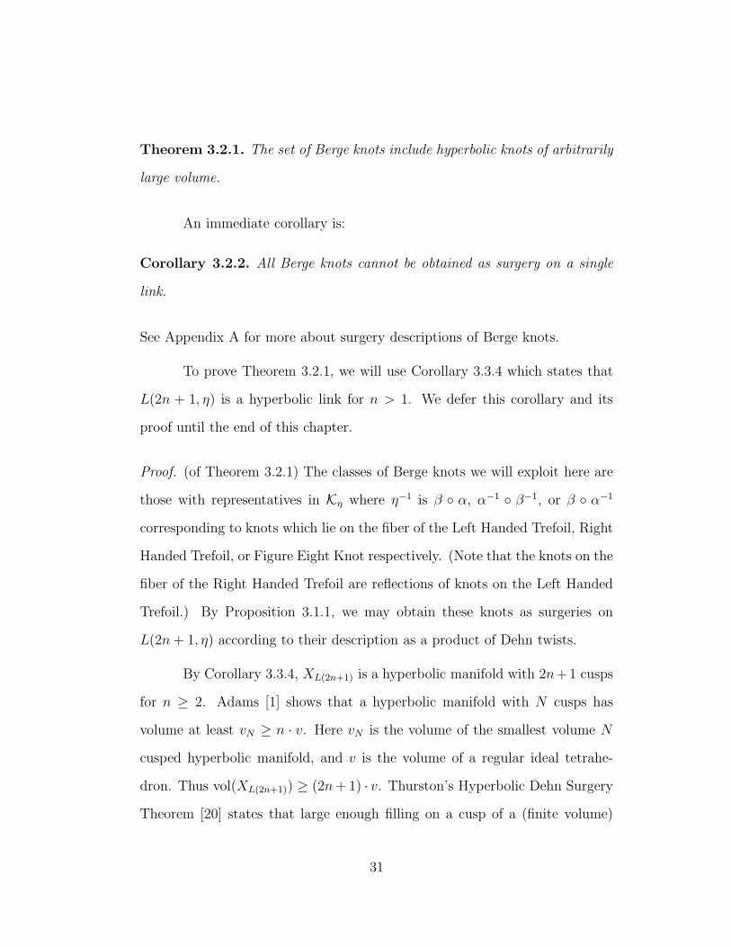
Definition 3.3.1. For n ∈ N, let C(2n+ 1) =n∪i=1Ci be the minimally twisted
chain link of 2n + 1 components as shown for each n even and n odd in
Figure 3.4. Note there are actually two such links, C(2n+1) and its reflection
−C(2n+ 1), depending on how the clasping of Cn and C−n is done. For each
i ∈ −n, . . . , n, let mi, li be the standard meridian-longitude pair for Ci.
In this section we will show
Theorem 3.3.1. The links L(2n + 1, η) and C(2n + 1) have homeomorphic
exteriors. I.e. XL(2n+1,η)∼= XC(2n+1).
Consequentially, we will use this homeomorphism to obtain descrip-
tions of the knots K ∈ Kη as surgeries on these chain links. Through different
methods Yuichi Yamada [22] has also obtained descriptions of many of these
32
C0
C1
C−1
C2
C−2
Cn
C−n
C−n+1
Cn−1
n odd
C0
C1
C−1
C2
C−2
Cn
C−n
C−n+1
Cn−1
n even
Figure 3.4: The minimally twisted 2n+ 1 chain for n even and n odd.
knots as surgeries on minimally twisted chain links. In Appendix A we de-
scribe the remaining Berge knots as surgeries on the minimally twisted five
chain link, MT5C = C(5). Furthermore, though it may be done directly, this
homeomorphism simplifies the proof of the hyperbolicity of L(2n+ 1).
33
3.3.1 Proof of Theorem 3.3.1
The following proof employs tangles. See Section 2.1.2 for the relevant defini-
tions.
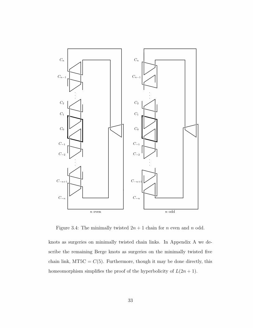
Throughout this subsection and the next, the choice of ε = ±1 depends
on the choice of η. This is encapsulated by
η−1 = β αε
so that ε = +1 corresponds to the Left Handed Trefoil and ε = −1 corresponds
to the Figure Eight Knot. Furthermore, in the ensuing figures, blocks with 12ε
indicate the half twists as shown in Figure 3.5.
ε = +1 ε = −1ε = +1 ε = −1
and
12
ε12
ε
Figure 3.5: Twistings of 12ε for ε = ±1.
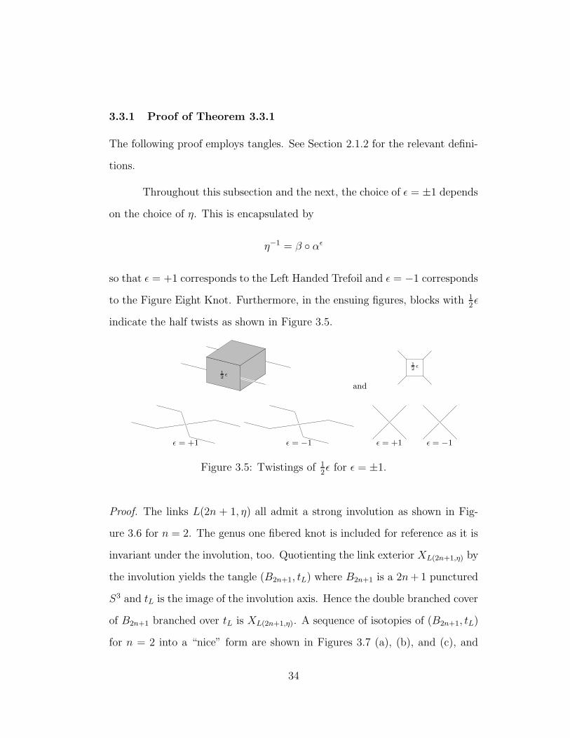
Proof. The links L(2n + 1, η) all admit a strong involution as shown in Fig-
ure 3.6 for n = 2. The genus one fibered knot is included for reference as it is
invariant under the involution, too. Quotienting the link exterior XL(2n+1,η) by
the involution yields the tangle (B2n+1, tL) where B2n+1 is a 2n+ 1 punctured
S3 and tL is the image of the involution axis. Hence the double branched cover
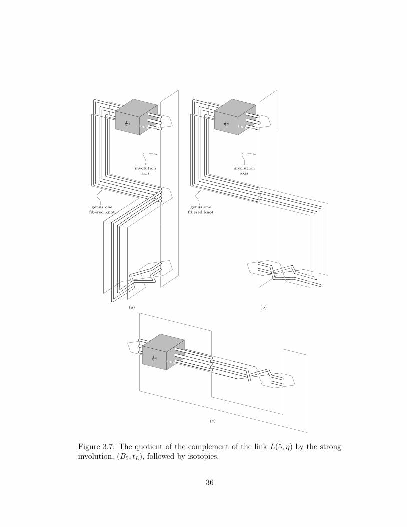
of B2n+1 branched over tL is XL(2n+1,η). A sequence of isotopies of (B2n+1, tL)
for n = 2 into a “nice” form are shown in Figures 3.7 (a), (b), and (c), and
34
involution
axis
genus one
fibered knot
12
ε
12
ε
Figure 3.6: The link L(5, η) with an axis of strong involution and the genusone fibered knot.
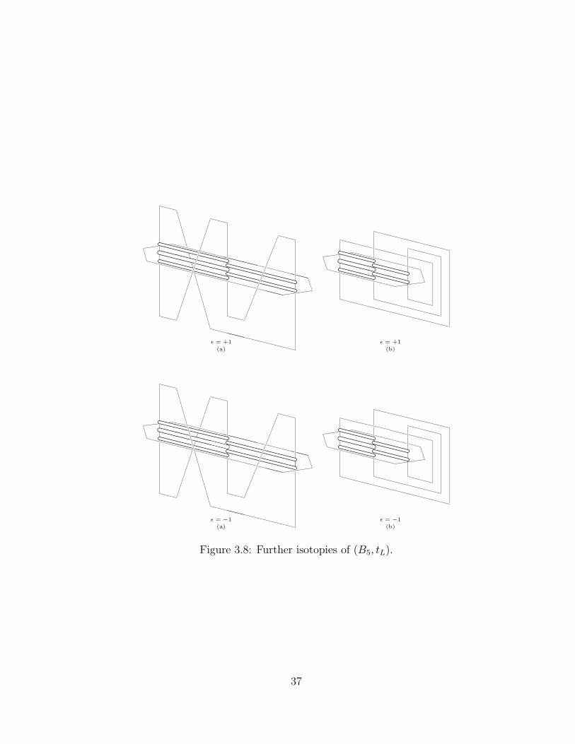
are continued in Figures 3.8 (a) and (b) with each choice of ε. The quotient
of the genus one fibered knot is also shown in these figures.
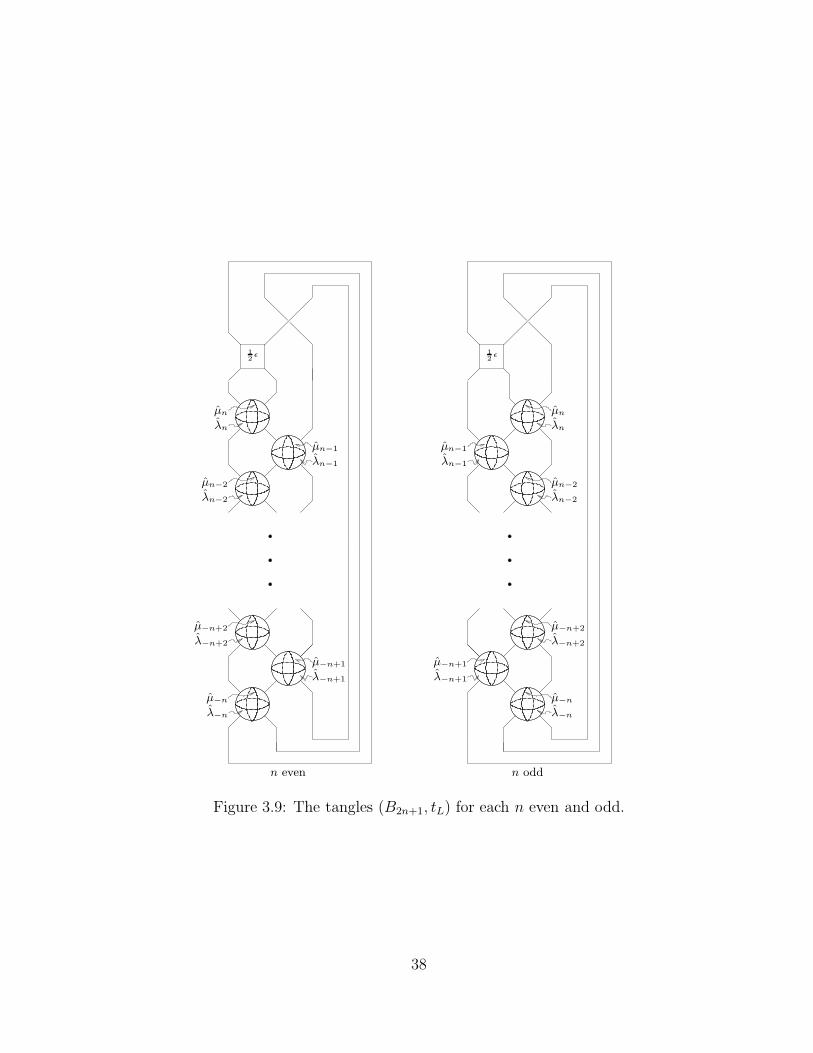
We may trace the longitudes λi and standard meridians µi of ∂N(Li)
through the quotient of XL(2n+1,η) and its subsequent isotopies as in Fig-
ures 3.6, 3.7, and 3.8 to obtain the corresponding framings λi and µi on the
ith boundary components ∂N(Li) of ∂(B2n+1, tL). The picture of (B2n+1, tL)
for general n with framings is shown in Figure 3.9.
The minimally twisted chain links C(2n+1) all admit strong involutions
35
involution
axis
genus one
fibered knot
involution
axis
genus one
fibered knot
(b)(a)
(c)
12
ε 12
ε
12
ε
Figure 3.7: The quotient of the complement of the link L(5, η) by the stronginvolution, (B5, tL), followed by isotopies.
36
ε = +1
(b)
ε = +1
(a)
(b)
ε = −1ε = −1
(a)
Figure 3.8: Further isotopies of (B5, tL).
37
n oddn even
µ−n+2
λ−n+2
µ−n
λ−n
µ−n+1
λ−n+1
µn
λn
µn−2
λn−2
µn−1
λn−1
µn
λn
µn−2
λn−2
µn−1
λn−1
µ−n+2
λ−n+2
µ−n
λ−n
µ−n+1
λ−n+1
12
ε12
ε
Figure 3.9: The tangles (B2n+1, tL) for each n even and odd.
38
(a) (b)
involutionaxis
C0
C1
C−1
C−2
C2
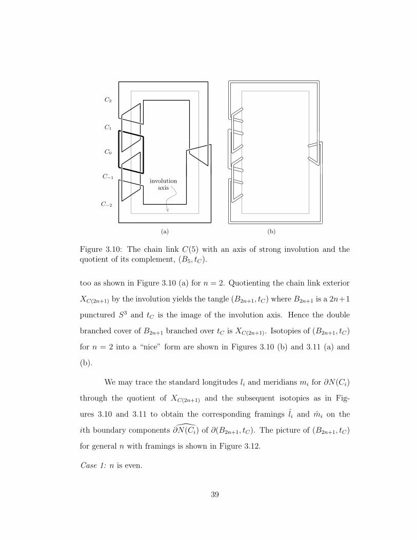
Figure 3.10: The chain link C(5) with an axis of strong involution and thequotient of its complement, (B5, tC).
too as shown in Figure 3.10 (a) for n = 2. Quotienting the chain link exterior
XC(2n+1) by the involution yields the tangle (B2n+1, tC) where B2n+1 is a 2n+1
punctured S3 and tC is the image of the involution axis. Hence the double
branched cover of B2n+1 branched over tC is XC(2n+1). Isotopies of (B2n+1, tC)
for n = 2 into a “nice” form are shown in Figures 3.10 (b) and 3.11 (a) and
(b).
We may trace the standard longitudes li and meridians mi for ∂N(Ci)
through the quotient of XC(2n+1) and the subsequent isotopies as in Fig-
ures 3.10 and 3.11 to obtain the corresponding framings li and mi on the
ith boundary components ∂N(Ci) of ∂(B2n+1, tC). The picture of (B2n+1, tC)
for general n with framings is shown in Figure 3.12.
Case 1: n is even.
39

(a) (b)
Figure 3.11: Isotopies of (B5, tC).
Figure 3.13 indicates a homeomorphism h between the two tangles
(B2n+1, tL) and (B2n+1, tC). The nth and −nth boundary components of
(B2n+1, tL) may absorb the extra twists into their framings as shown in Fig-
ure 3.14 to complete the homeomorphism.
The homeomorphism
h : (B2n+1, tL) → (B2n+1, tC)
then lifts to a homeomorphism
h : XL(2n+1,η) → XC(2n+1)
of the double branched covers.
Case 2: n is odd.
The result of further isotopies of the tangles (B2n+1, tL) and (B2n+1, tC)
as depicted in Figures 3.9 and 3.12 for n odd are shown together in Figure 3.15
40
n even n odd
lnmn
ln−2
mn−2
ln−1
mn−1
l−n+2
m−n+2
l−n
m−n
l−n+1
m−n+1
lnmn
ln−2
mn−2
ln−1
mn−1
l−n+2
m−n+2
l−n
m−n
l−n+1
m−n+1
Figure 3.12: The tangles (B2n+1, tC) for each n even and odd.
41
(B2n+1, tC)
n even
(B2n+1, tL)
µn
λn
µn−2
λn−2
µn−1
λn−1
µ−n+2
λ−n+2
µ−n
λ−n
µ−n+1
λ−n+1
lnmn
ln−2
mn−2
ln−1
mn−1
l−n+2
m−n+2
l−n
m−n
l−n+1
m−n+1
12
ε
Figure 3.13: The tangles (B2n+1, tL) and (B2n+1, tC) for n even.
42
'h7→
µn
λn
µn
λn
lnmn
ε = −1:
'h7→
µ−n
λ−n
µ−n
λ−n
l−n
m−n
ε = ±1:
Figure 3.14: Twistings of the nth and −nth boundary components as neededfor h for n even.
suggesting a homeomorphism h. The isotopy of (B2n+1, tC) employs the “braid
relation move” of Figure 3.16.
If ε = +1, the nth boundary component may absorb an extra twist
into its framing as shown in Figure 3.17 to complete the homeomorphism h
between (B2n+1, tL) and (B2n+1, tC) indicated in Figure 3.15.
The homeomorphism
h : (B2n+1, tL) → (B2n+1, tC)
then lifts to a homeomorphism
h : XL(2n+1,η) → XC(2n+1)
of the double branched covers.
If ε = −1, take the reflection of (B2n+1, tC) through the plane of the
page. The resulting tangle (B2n+1, t−C) has the complement of −C(2n + 1)
43
(B2n+1, tL)
n odd
(B2n+1, tC)
n odd
µn
λn
µn−2
λn−2
µn−1
λn−1
µ−n+2
λ−n+2
µ−n
λ−n
µ−n+1
λ−n+1
lnmn
ln−2
mn−2
ln−1
mn−1
l−n+2
m−n+2
l−n
m−n
l−n+1
m−n+1
12
ε
Figure 3.15: The tangles (B2n+1, tL) and (B2n+1, tC) for n odd.
44

'
Figure 3.16: A braid isotopy.
'h7→
µn
λn
lnmn
µn
λn
Figure 3.17: Twisting of the nth boundary component as needed for h for nodd and ε = +1.
as its double branched cover. The nth and −nth boundary components of
(B2n+1, tL) may absorb the extra twists into their framings as shown in Fig-
ure 3.18 to complete the homeomorphism h between (B2n+1, tL) and (B2n+1, t−C).
The homeomorphism
h : (B2n+1, tL) → (B2n+1, t−C)
then lifts to a homeomorphism
h : XL(2n+1,η) → X−C(2n+1)
of the double branched covers.
45

'h7→
'h7→
µn
λn
µn
λn
µ−n
λ−n
µ−n
λ−n
l−n
m−n
ln
mn
Figure 3.18: Twisting of the nth and −nth boundary components as neededfor h for n odd and ε = −1.
3.3.2 Surgeries on chain links.
The homeomorphisms h in the proof of Theorem 3.3.1 describe how the framed
boundary components of (B2n+1, tL) map to the framed boundary components
of (B2n+1, t±C). In the lift to the double branched covers, this confers how
the homeomorphism h maps the boundary components of XL(2n+1,η) to the
boundary components of X±C(2n+1) in terms of their corresponding meridian-
longitude basis pairs. We thereby obtain mappings of slopes and translate
surgery coefficients for L(2n + 1, η) to surgery coefficients for ±C(2n + 1).
In the following maps, for each i ∈ −n, . . . , n the curves µi and λi on
∂N(Li) and the curves mi and li on ∂N(Ci) are thought of synonymously with
their homological representatives so that we may add and subtract them to
produce other curves on these tori. Furthermore these maps should be taken
up to reversal of orientations of pairs mi, li.
46
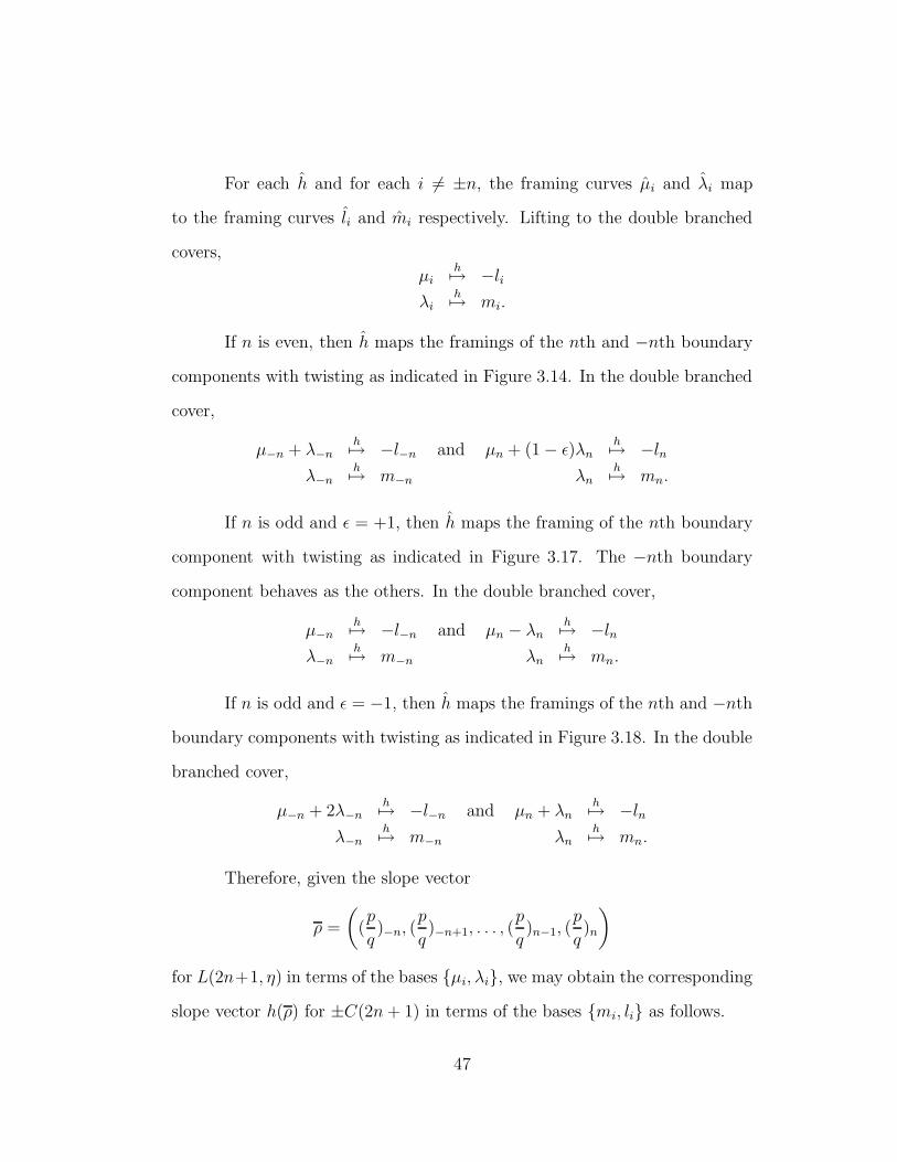
For each h and for each i 6= ±n, the framing curves µi and λi map
to the framing curves li and mi respectively. Lifting to the double branched
covers,
µih7→ −li
λih7→ mi.
If n is even, then h maps the framings of the nth and −nth boundary
components with twisting as indicated in Figure 3.14. In the double branched
cover,
µ−n + λ−nh7→ −l−n and µn + (1 − ε)λn
h7→ −ln
λ−nh7→ m−n λn
h7→ mn.
If n is odd and ε = +1, then h maps the framing of the nth boundary
component with twisting as indicated in Figure 3.17. The −nth boundary
component behaves as the others. In the double branched cover,
µ−nh7→ −l−n and µn − λn
h7→ −ln
λ−nh7→ m−n λn
h7→ mn.
If n is odd and ε = −1, then h maps the framings of the nth and −nth
boundary components with twisting as indicated in Figure 3.18. In the double
branched cover,
µ−n + 2λ−nh7→ −l−n and µn + λn
h7→ −ln
λ−nh7→ m−n λn
h7→ mn.
Therefore, given the slope vector
ρ =
((p
q)−n, (
p
q)−n+1, . . . , (
p
q)n−1, (
p
q)n
)
for L(2n+1, η) in terms of the bases µi, λi, we may obtain the corresponding
slope vector h(ρ) for ±C(2n+ 1) in terms of the bases mi, li as follows.
47
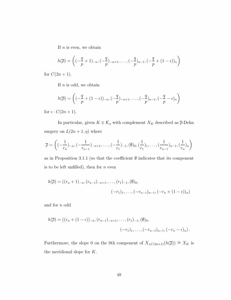
If n is even, we obtain
h(ρ) =
((−
q
p+ 1)−n, (−
q
p)−n+1, . . . , (−
q
p)n−1, (−
q
p+ (1 − ε))n
)
for C(2n+ 1).
If n is odd, we obtain
h(ρ) =
((−
q
p+ (1 − ε))−n, (−
q
p)−n+1, . . . , (−
q
p)n−1, (−
q
p− ε)n
)
for ε · C(2n+ 1).
In particular, given K ∈ Kη with complement XK described as ρ-Dehn
surgery on L(2n + 1, η) where
ρ =
((−
1
rn)−n, (−
1
rn−1)−n+1, . . . , (−
1
r1)−1, (∅)0, (
1
r1)1, . . . , (
1
rn−1)n−1, (
1
rn)n
)
as in Proposition 3.1.1 (so that the coefficient ∅ indicates that its component
is to be left unfilled), then for n even
h(ρ) = ((rn + 1)−n, (rn−1)−n+1, . . . , (r1)−1, (∅)0,
(−r1)1, . . . , (−rn−1)n−1, (−rn + (1 − ε))n)
and for n odd
h(ρ) = ((rn + (1 − ε))−n, (rn−1)−n+1, . . . , (r1)−1, (∅)0,
(−r1)1, . . . , (−rn−1)n−1, (−rn − ε)n) .
Furthermore, the slope 0 on the 0th component of X±C(2n+1)(h(ρ)) ∼= XK is
the meridional slope for K.
48
3.3.3 Hyperbolicity of the links L(2n + 1, η).
Corollary 3.3.2. (of [15], Theorem 5.1 (ii).) The links C(2n+1) are hyperbolic
for n > 1.
Proof. This is an immediate corollary of
Theorem 3.3.3. (Theorem 5.1 (ii) of Neumann-Reid [15]) C(p, s) has a hyper-
bolic structure (complete of finite volume) if and only if |p+s|, |s| 6⊂ 0, 1, 2.
Our links C(2n + 1) correspond to their links C(2n+ 1,−n− 1) or
C(2n+ 1,−n) depending on how the last clasping is done. Since n > 1 the
theorem applies.
From the above homeomorphism of link exteriors and corollary, we
conclude
Corollary 3.3.4. L(2n + 1, η) is a hyperbolic link for n ≥ 2.
49

Chapter 4
Closed Essential Surfaces
In this chapter we develop an algorithm to list all the closed essential surfaces
in the complement of any given knot in S3 that belongs to Kη. We first develop
an algorithm to list all the surfaces in once-punctured torus bundle that are
both disjoint from a given level knot and essential its complement. Then
we determine when Dehn filling the boundary of the once-punctured torus
bundle permits a surface to cap off to a closed surface which is essential in the
complement of the knot. We take lead from the work Incompressible surfaces in
once-punctured torus bundles by Culler-Jaco-Rubinstein [6] which constructs
an algorithm to list surfaces as in the title and adapt their methods to our
situation. We assume familiarity with this paper throughout this chapter.
4.1 Twisted Surfaces
We begin by describing a certain type of surface in once-punctured torus bun-
dles and in the complement of a level knot in a once-punctured torus bundle.
Much of the terminology and methods used here are borrowed or adapted from
[6].
50
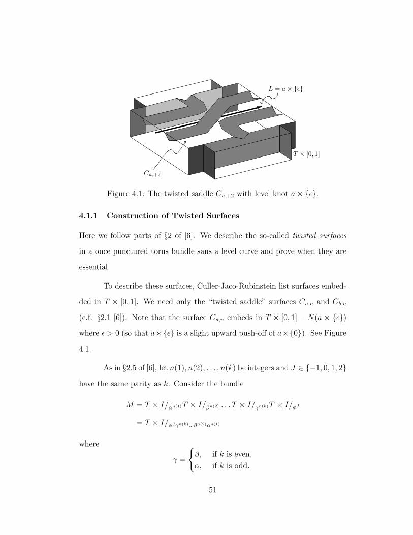
L = a × ε
Ca,+2
T × [0, 1]
Figure 4.1: The twisted saddle Ca,+2 with level knot a× ε.
4.1.1 Construction of Twisted Surfaces
Here we follow parts of §2 of [6]. We describe the so-called twisted surfaces
in a once punctured torus bundle sans a level curve and prove when they are
essential.
To describe these surfaces, Culler-Jaco-Rubinstein list surfaces embed-
ded in T × [0, 1]. We need only the “twisted saddle” surfaces Ca,n and Cb,n
(c.f. §2.1 [6]). Note that the surface Ca,n embeds in T × [0, 1] − N(a × ε)
where ε > 0 (so that a×ε is a slight upward push-off of a×0). See Figure
4.1.
As in §2.5 of [6], let n(1), n(2), . . . , n(k) be integers and J ∈ −1, 0, 1, 2
have the same parity as k. Consider the bundle
M = T × I/αn(1)T × I/βn(2) . . . T × I/γn(k)T × I/φJ
= T × I/φJγn(k)...βn(2)αn(1)
where
γ =
β, if k is even,
α, if k is odd.
51
Note that M contains k + 1 blocks. Take L = a× ε in the first block of M
for small ε > 0. (We may actually think of L as being a×0, but it is useful
to have L not on a fiber along which blocks of M are glued.)
Construct the surface R by putting twisted saddles in the first k blocks
of M , Ca,n(i) if i is odd and Cb,n(i) if i is even, and the vertical disks a± × I
or b± × I in the (k + 1)th block of M . These surfaces fit together to make
a properly embedded connected surface R which is disjoint from L. R is
orientable if k is even and non-orientable if k is odd.
For an example of how these twisted saddles fit together to give a
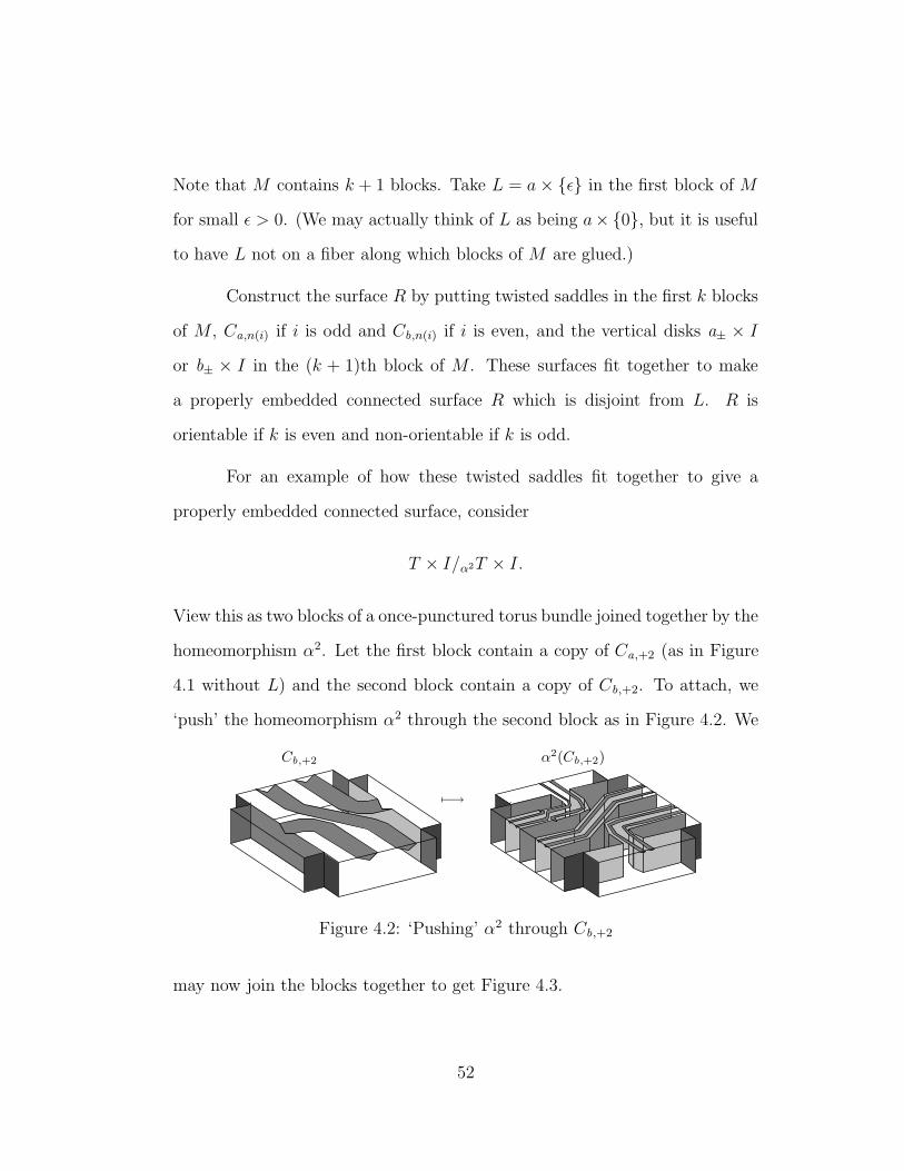
properly embedded connected surface, consider
T × I/α2T × I.
View this as two blocks of a once-punctured torus bundle joined together by the
homeomorphism α2. Let the first block contain a copy of Ca,+2 (as in Figure
4.1 without L) and the second block contain a copy of Cb,+2. To attach, we
‘push’ the homeomorphism α2 through the second block as in Figure 4.2. We
Cb,+2 α2(Cb,+2)
7−→
Figure 4.2: ‘Pushing’ α2 through Cb,+2
may now join the blocks together to get Figure 4.3.
52
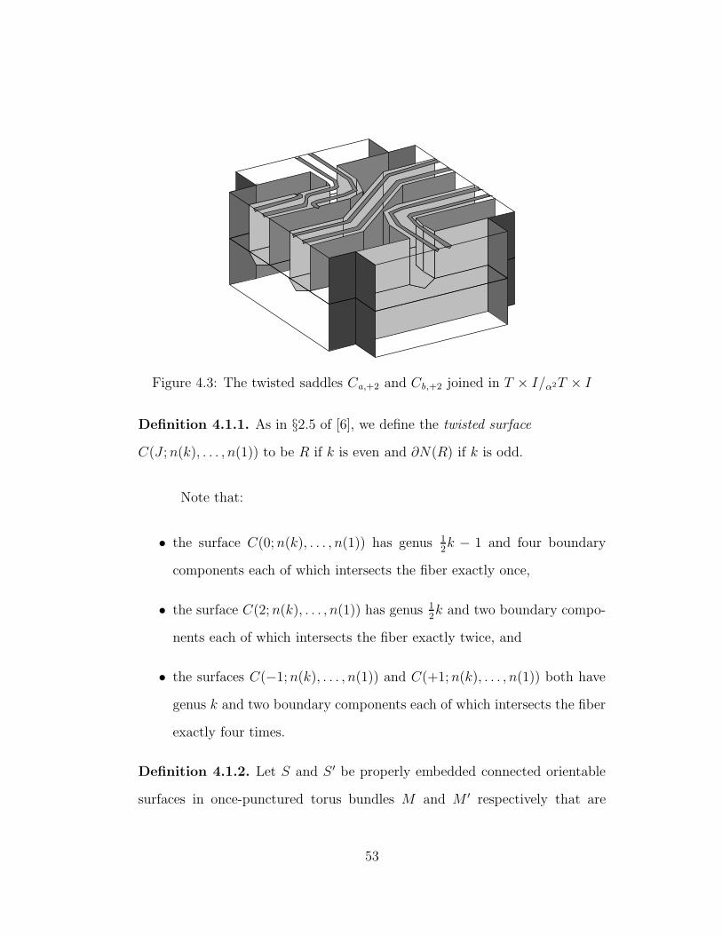
Figure 4.3: The twisted saddles Ca,+2 and Cb,+2 joined in T × I/α2T × I
Definition 4.1.1. As in §2.5 of [6], we define the twisted surface
C(J ;n(k), . . . , n(1)) to be R if k is even and ∂N(R) if k is odd.
Note that:
• the surface C(0;n(k), . . . , n(1)) has genus 12k − 1 and four boundary
components each of which intersects the fiber exactly once,
• the surface C(2;n(k), . . . , n(1)) has genus 12k and two boundary compo-
nents each of which intersects the fiber exactly twice, and
• the surfaces C(−1;n(k), . . . , n(1)) and C(+1;n(k), . . . , n(1)) both have
genus k and two boundary components each of which intersects the fiber
exactly four times.
Definition 4.1.2. Let S and S ′ be properly embedded connected orientable
surfaces in once-punctured torus bundles M and M ′ respectively that are
53
disjoint from essential level knots L and L′ respectively. Then we say S and
S ′ are of the same type if there is a bundle equivalence from M to M ′ that
maps S to S ′ and L to L′. (C.f. §2.6 of [6].)
Remark 4.1.1. If the bundle M contains a surface of type C(J ;n(k), . . . , n(1)),
then M has the characteristic class
[P JBn(k) . . . Bn(2)An(1)].
4.1.2 Essential Twisted Surfaces
Proposition 4.1.1. (c.f. Proposition 2.5.1 [6]) Let J , n(1), n(2), . . . , n(k),
L, and M be as above. The surface C(J ;n(k), . . . , n(2), n(1)) is essential in
M −N(L) if and only if |n(i)| ≥ 2 for i = 2, . . . , k.
Proof. We cite the proof of Proposition 2.5.1 [6] and show only the parts where
we must diverge. We begin by reestablishing notation.
Let M be the cyclic cover, corresponding to the fiber, of the bundle
M = T × I/αn(1)T × I/βn(2) . . . T × I/ϕJ .
Let L be the inverse image of L under the covering projection and
S ⊂ M −N(L) ⊂ M
be a component of the inverse image of
C(J ;n(k), . . . , n(1)) ⊂ M −N(L) ⊂M
under the covering projection. As noted in [6], it suffices to show that S is
incompressible in M −N(L). Furthermore M is divided into blocks which are
54
inverse images of the blocks of M , and each block in M meets S in one disk
as in Fig. 4 of [6]. Let F be the union of the fibers along which the blocks in
M are joined.
We want to consider the family of all compressing and boundary com-
pressing disks for S in M −N(L). This is equivalent to considering the family
of compressing disks for S in M that are disjoint from L. We first, however,
consider the family of all compressing and boundary compressing disks for S
in M (regardless of L). By Proposition 2.5.1 of [6], this family is non-empty
if and only if |n(i)| < 2 for some i = 1, . . . , k.
From the proof of Proposition 2.5.1, such a minimal disk is contained
in the solid torus formed by cutting two adjacent blocks of M along S and
joining two of the resulting solid torus components along the annulus of their
common intersection with F . If the two blocks are preimages of the (i− 1)th
(modulo k) and ith blocks of M under the covering projection, then |n(i)| < 2
if and only if such a disk exists in this solid torus. The disk is isotopic to a
meridional disk of the solid torus and non-trivially intersects the core of the
solid torus. In the case that |n(1)| < 2, a component of L is contained in this
solid torus (since it is isotopic to the core of the gluing annulus) and is isotopic
to its core. Thus it will non-trivially intersect the disk.
As stated in Remark 2.5.2 of [6], a stronger statement than that of the
above proposition is true. We will need this stronger statement and hence
prove it here.
55
Theorem 4.1.2. (c.f. Remark 2.5.2 [6]) Let J, n(1), n(2), . . . , n(k), L and M
be as above. Let M be the manifold constructed by attaching a solid torus
to M so that the boundary curves of C(J ;n(k), . . . , n(2), n(1)) are identi-
fied to contractible curves in the solid torus. Let C(J ;n(k), . . . , n(2), n(1))
be the surface in M obtained by attaching disks to the boundary curves of
C(J ;n(k), . . . , n(2), n(1)). Then C(J ;n(k), . . . , n(2), n(1)) is essential in
M −N(L) if and only if |n(i)| ≥ 2 for i = 2, . . . , k.
Proof. We will first prove this only in the case that J = 0 or 2. Afterwards
we will address the case that J = ±1.
Let C = C(J ;n(k), . . . , n(2), n(1)) and C = C(J ;n(k), . . . , n(2), n(1)).
If J = 0 or 2, then each block meets C in a single disk as in Fig. 4 of [6]. If
J = ±1, then each block meets C in two disks which are a parallel, each of
which individually appears as in Fig 4. of [6]. Let F be the union of the fibers
along which the blocks of M are joined.
Let K be the core of the surgered torus so that M − N(K) = M .
Consider the family of all compressing disks for C in M −N(L). If this family
is non-empty then there exists a member D for which (D ∩ K,D ∩ F ) is
minimized lexicographically. We may assume D transversely intersects K.
Due to Proposition 4.1.1, D∩K 6= ∅. Let P = D−N(K) ⊂M −N(L)
be the punctured disk which has one boundary component, say ∂P0 = ∂D, on
C and all other boundary components on ∂N(K) parallel to ∂C. Note that P
is incompressible in M −N(L) due to the minimality assumption on D.
First we observe that there cannot be any simple closed curve compo-
nents of P ∩ F contractible on F . If there is, then there is one, say σ ′, which
56

is innermost on F . Thus σ′ bounds a disk ∆ ⊂ F . Surgering P along ∆ yields
two surfaces one of which, say P ′, has ∂D as a boundary component. P ′ then
completes to a compressing disk D′ for C in M −N(L) with ∂D′ = ∂D. Fur-
thermore |D′ ∩ K| ≤ |D ∩ K| and |D′ ∩ F | < |D ∩ F |. This contradicts the
minimality assumption on D.
Part I. J = 0 or 2
Let X be a block of MK with ∂P0 ∩X 6= ∅. Cutting X along C yields
two solid tori as shown in Fig. 6 of [6]. Consider one of the solid tori which has
non-empty intersection with ∂P0. As before (at the beginning of this proof)
its boundary meets C in a disk, ∂M in two disks (labelled B), and F in a disk,
Fd, and an annulus, Fa. Note that ∂P0 need not intersect Fd.
Suppose that σ is an arc component of P ∩Fd. There are four cases for
such an arc that we need to consider.
Case 1. Both end points of σ are on the same component of B ∩ Fd.
Here σ is an arc with both end points in ∂P − ∂D ⊂ ∂M . Among all the
components of P ∩ Fd that have both end points on the same component of
B ∩ Fd, choose one, say σ′, that is outermost on Fd. Thus there is a disk
∆ ⊂ Fd such that ∂∆ consists of two arcs, σ′ and δ′ where δ′ ⊂ R ∩ Fd and
∆ ∩ P = σ′. δ′ is an arc on ∂M connecting two distinct components of ∂P
on ∂M . Let Q be the annulus of ∂M connecting these two components that
contains δ′. Surgering P along ∆ ∪ Q yields a planar surface P ′ such that
∂D ⊂ ∂P ′. Then in ML P ′ completes to a compressing disk D′ for which
|D′ ∩K| < |D ∩K| contradicting the minimality assumption on D.
Case 2. Both end points of σ are on the same component of C ∩ Fd.
57

Here σ is an arc with both end points in ∂D ⊂ C. Among all the components
of P ∩Fd that have both end points on the same component of C ∩Fd, choose
one, say σ′, that is outermost on Fd. Thus there is a disk ∆ ⊂ Fd such that ∂∆
consists of two arcs, σ′ and δ′ where δ′ ⊂ R ∩ Fd and ∆ ∩ P = σ′. Surgering
P along ∆ yields two planar surfaces each with one boundary component
on C and the rest on ∂M . Both of these planar surfaces complete to disks,
say D′ and D′′ in ML with boundary in C. Both of these disks have fewer
intersections with F and no more intersections with K than D. At least one
of the boundaries of these disks, say D′, must be essential in C. Thus D′ is a
compressing disk for C contradicting the minimality assumption on D.
Case 3. One end point of σ is contained in B and one is contained in
C. On P , σ must connect ∂D with another boundary component of P . Since
neither Case 1 nor Case 2 occur, we may choose among all the components of
P ∩ Fd with one end point in B and one end point in C an arc, say σ′, that is
outermost on Fd. Thus there is a disk ∆ ⊂ Fd such that ∂∆ is the union of
three consecutive arcs σ′, r′ ⊂ C, and δ′ ⊂ B, and ∆ ∩ P = σ′. δ′ connects a
component of ∂P and ∂C on ∂M . Let Q be the annulus of ∂M between these
two components that contains δ′. Surger P along ∆∪Q to yield a surface P ′.
In M , P ′ completes to a disk D′ with ∂D′ isotopic to ∂D in C. Thus D′ is a
compressing disk for C. Furthermore, |D′ ∩ K| < |D ∩ K| contradicting the
minimality assumption on D.
Case 4. One end point of σ is contained in one component of C ∩ Fd
and the other end point is contained in the other component of C ∩Fd. On P ,
σ has both end points on ∂D ⊂ C. In Fd, the arc σ is parallel in Fd into an
58

arc component of Fd ∩ B. Since none of the Cases 1, 2, or 3 occur, among all
the components of P ∩ Fd with end points in C ∩ Fd there is one, say σ′, that
is outermost on Fd. Thus there is a disk ∆ ⊂ Fd such that ∂∆ is the union
of four consecutive arcs σ′, r′ ⊂ C, δ′ ⊂ B, and r′′ ⊂ C, and ∆ ∩ P = σ′. δ′
connects two components of ∂C on ∂M . Let Q be the annulus of ∂M between
these two components that contains δ′. Surger P along ∆∪Q to yield a surface
P ′. In M P ′ completes to a disk D′ with ∂D′ isotopic to ∂D in C. Thus D′ is
a compressing disk for C. Furthermore, |D′ ∩K| < |D ∩K| contradicting the
minimality assumption on D.
Note that there is fifth possible arc type for σ: One end point of σ is
contained in one component of B ∩ Fd and the other end point is contained
in the other component of B ∩ Fd. We need not address this case for our
purposes.
Let X ′ denote the block in M that meets the block X along the com-
ponent of F containing Fa. X ′ splits into two solid tori as X did, and the
same arguments of Cases 1, 2, 3, and 4 for X apply to X ′. Joining X and X ′
along the annulus Fa forms a solid torus V which meets C in an annulus that
wraps around the solid torus |n(i)| times for some i.
Note that as a consequence of Cases 2, 3, and 4, Fd∩∂P0 = ∅. Therefore
∂P0 is contained in the annulus C ∩ V and is thus isotopic to the core of this
annulus.
Consider the component Q of P ∩ V that contains ∂P0. Since P is
incompressible in M − N(L), then Q must be incompressible in V − N(L)
which is either a solid torus or a torus cross interval depending on whether
59
L is contained in V . Since the only incompressible surfaces in a solid torus
are meridional disks and boundary parallel annuli, either Q is one of these if
L 6⊂ V or Q is a boundary parallel annulus if L ⊂ V .
Case A. AssumeQ is a boundary parallel annulus. Since one component
of ∂Q is ∂P0 the other component does not intersect C. Let σ be an arc of
Q∩Fa and ∆ be the disk in Fa with ∂∆ = σ ∪ (∆∩ ∂V ). Thus σ has one end
point in C and one end point in B. Hence σ is an arc like in Case 3. Since
Cases 1, 2, and 3 may apply to arcs of P ∩∆ in ∆, the existence of σ yields a
contradiction.
Case B. Assume Q is a meridional disk. Such a disk can only occur if
n(i) = 0 which cannot be the case unless i = 1. However, if i = 1, then L ⊂ V
and then L ∩Q 6= ∅ which is a contradiction.
Part II. J = ±1
Again, let X be a block of MK with ∂P0 ∩ X 6= ∅. Cutting X along
C yields two solid tori as shown in Fig. 6 of [6] as well as one product disk
(∼= D2 × I) that gives the parallelism between the two disk components of
X ∩ C.
The arguments of Part I apply to these solid torus components. There-
fore we only need consider the case that the product disk has non-empty in-
tersection with ∂P0. The boundary of the product disk meets C in two disks,
∂M in four disks (labelled B), and F in four disks.
Each disk component of the intersection of the product disk and F
is a rectangle with two edges on C and two edges on B. Consider one of
these components which has non-empty intersection with ∂P0 and call it Fd.
60

Cases 1, 2, 3, and 4 of Part I all then apply to the arcs of P ∩ Fd. Therefore
Fd ∩ ∂P0 = ∅. Thus ∂P0 must be contained in this product disk. But this
cannot occur as then ∂P0 would be contained in a disk of C and hence bound
a disk in C.
Definition 4.1.3. We may say that a surface S0 in M − N(L) has the same
type as C(J ;n(k), . . . , n(2), n(1)) if it is isotopic to C(J ;n(k), . . . , n(2), n(1))
in M −N(L).
Remark 4.1.2. Continuing with the notation above, if M ∼= S3 and |n(i)| ≥ 2
for i = 2, . . . , k, then L is a knot in S3 and C(J ;n(k), . . . , n(2), n(1)) is a
closed essential surface in the complement of L, XL = S3 −N(L).
4.1.3 Classification of Essential Twisted Surfaces
A given once-punctured torus bundle with an essential level knot may contain
several surfaces essential in the complement of the level knot which are have
the type of a twisted surface. We may determine when two are in the same
isotopy class. This is effectively done in §4.1 of [6].
Recall that if M is a fiber bundle, then an isotopy of M which is a
bundle equivalence at each time is called a bundle isotopy.
Proposition 4.1.3. Let M be a once-punctured torus bundle containing sur-
faces S and S ′ of types C(J ;n(k), . . . , n(1)) and C(J ′;m(k′), . . . , m(1)), re-
spectively, that are disjoint from an essential level curve L. Then S and
S ′ are isotopic in the complement of L if and only if k = k′, J = J ′, and
61
(m(k), . . . , m(1)) = (n(k), . . . , n(1)). Moreover there is a bundle isotopy tak-
ing (S, L) to (S ′, L).
Proof. This follows directly from the proof of Proposition 4.1.3 of [6]. Note
that because of L, we get that (m(k), . . . , m(1)) and (n(k), . . . , n(1)) are re-
lated by equality rather than cyclic permutation.
We now relate essential twisted surfaces in a based once-punctured
torus bundle to certain expressions of the bundle’s characteristic class (c.f.
Remark 4.1.1).
Proposition 4.1.4. Let L be an essential level curve in a once-punctured torus
bundle M . Assume M = T ×I/η such that L is contained in T ×0. Assume
η is identified with H ∈ SL2(Z). Then for each element W ∈ SL2(Z) such that
W [a] = [L]: if W−1HW may be expressed as a special form
P JAn(k) . . . Bn(2)An(1), where J ∈ +1,−1 and |n(i)| ≥ 2 for i = 2, . . . , k
or
P JBn(k) . . . Bn(2)An(1), where J ∈ 0, 2 and |n(i)| ≥ 2 for i = 2, . . . , k
then there is an essential surface in M −N(L) of type C(J ;n(k), . . . , n(1)).
Proof. Let ω be the homeomorphism of T associated to W . Then ω naturally
extends to a bundle equivalence
ω : M ′ = T × I/ω−1ηω →M = T × I/η
62

such that ω(a) = L. If W−1HW may be expressed as the special form
P J . . . Bn(2)An(1) then
ω−1 η ω = φJ . . . βn(2)αn(1).
Thus
M ′ = T × I/ω−1ηω = T × I/φJ ...βn(2)αn(1) ,
and so M ′ contains the twisted surface C(J ;n(k), . . . , n(2), n(1)). Since
P J . . . Bn(2)An(1) is a special form, |n(i)| ≥ 2 for i = 2, . . . , k, and hence the
surface C(J ;n(k), . . . , n(2), n(1)) is essential in the complement of a× 0.
Therefore ω(C(J ;n(k), . . . , n(2), n(1))) is an essential surface in
M −N(L) = ω(M ′) −N(ω(a))
of type C(J ;n(k), . . . , n(2), n(1)).
Together, Propositions 4.1.3 and 4.1.4 give us
Corollary 4.1.5. Let M , L, and H be as above. The essential surfaces in
M −N(L) with the type of a twisted surface are in one-to-one correspondence
with special forms of conjugates W−1HW of H where W ∈ SL2(Z) such that
W [a] = [L].
4.2 Structure of Surfaces
This section closely follows §3 of [6]. Many of their arguments are easily
modified to accommodate the presence of an essential level knot L in a once-
punctured torus bundle M . Parts that do not involve L will be simply cited.
63
Let S be a properly embedded surface in M that is disjoint from L and
essential in M −N(L). We will say that S is in general position provided that
1. each component of ∂S is either contained in a fiber or is transverse to
every fiber,
2. the projection p : M → S1 restricts to a Morse function on the interior
of S having distinct critical values different from p(L),
3. among all surfaces isotopic to S in M −N(L) and satisfying (1) and (2),
S has the minimal number of index 0 or 2 critical points.
We may assume that S has been moved by an isotopy with support outside
of a neighborhood of L to be in general position. The level sets of p|S are the
intersections of S with the fibers of M .
Let x be a critical point. We use the following terms as defined in
section 3 of [6]: level arcs, level sets, critical neighborhood of x, and upper and
lower level sets of x. We let X be the critical neighborhood of x. We then
have the following lemmas:
Lemma 4.2.1. (3.1.1 of [6]) Each level arc of S is essential in the fiber con-
taining it.
Lemma 4.2.2. (3.2.1 of [6]) Either S meets every non-critical fiber only in
arcs or S meets every non-critical fiber only in simple closed curves.
Lemma 4.2.3. (3.2.2 of [6]) If both the upper and lower level sets of X contain
an essential closed curve, then these curves are isotopic.
64

Lemma 4.2.4. (3.2.3 of [6]) If the lower level set contains two arcs then
1. they are parallel, and
2. the upper level set is obtained by a band sum across the annulus compo-
nent of the complement.
Proof. All four lemmas follow almost exactly as in [6].
One needs for the proof of Lemma 4.2.2 that M −N(L) is irreducible.
This follows from the irreducibility of M and that L is non-trivial in its fiber.
Since critical points of S occur away from L, arguments involving crit-
ical neighborhoods are unchanged.
For the proof of Theorem 3.3.1 in [6], the authors employ a lemma due
to Haken [9]. For the upcoming proof of Theorem 4.2.6, we must alter the
lemma to accommodate the presence of L.
Lemma 4.2.5. Let T be a punctured torus, and let L be an essential, non-
boundary parallel simple closed curve in the fiber T × 12 of T × I. Let R be
a properly embedded, connected, incompressible surface in T × I −N(L) such
that each component of ∂R is contained in either ∂T × I, T ×0, or T ×1
and, in the latter two cases, parallel in its fiber to ∂T × I. Then R is either
an annulus, a once-punctured torus, or a torus parallel to ∂N(L).
Proof. R is disjoint from L in T × I. If R is incompressible in T × I, then
it follows from [9] that R is either an annulus or a once-punctured torus. So
assume R is compressible in T × I, and note that any compressing disk must
then intersect L.
65
We may assume that L = a × 12. Then let Aa be the annulus a× I,
and let Ab be the annulus b× I. Note that L is the core of Aa and intersects
Ab once.
By standard arguments, we may assume that R has been isotoped rel-∂
to minimize both |Aa ∩R| and |Ab ∩R|. It follows that Aa ∩R is a collection
of simple closed curves on Aa that are parallel to the core of Aa (and hence
L), and that Ab ∩ R is a collection of simple closed curves on Ab that either
bound disks in Ab that intersect L or are parallel to the core of Ab.
Case 1. Assume there exists a curve in Ab∩R that bounds a disk in Ab.
Among the curves of Ab ∩ R that bound disks in Ab, let c be the innermost.
Let Dc be the disk bounded by c. By minimality assumptions, we may assume
|c ∩ Aa| = 2. Thus there exists a curve in Aa, say c′, such that c ∩ c′ 6= ∅.
Note that c′ is innermost among Aa ∩R in the sense that if Ac′ is the annulus
between L and c′, then Ac′ ∩ R = c′. Consider δ = ∂N(c ∪ c′) ∩ R and the
subdisk ∆ of ∂N(Dc∪Ac′) that it bounds. Note that since ∆ is disjoint from L,
δ must bound a disk, say ∆′, in R. Furthermore, note that ∆′ ∩N(c∪ c′) = δ.
Thus R = ∆′ ∪N(c ∪ c′) which is a torus. This torus is parallel to ∂N(L).
Case 2. Assume now that there are no curves of Ab ∩ R that bound
disks in Ab. Thus all curves of Ab∩R are parallel to the core of Ab. Among the
compressing disks for R, let D be a compressing disk that |D∩Aa| is minimal.
Thus D ∩ Aa contains no simple closed curves. Note that D ∩ Aa 6= ∅ since
D ∩ L 6= ∅. Consider the arcs of D ∩ Aa. Due to the minimality assumptions
on D ∩ Aa and R ∩ Aa, every arc of D ∩ Aa crosses L.
Let d be an outermost arc on D of D∩Aa, and let D′ be the (outermost)
66
disk cut off by d. Let d′ be the arc of ∂D so that ∂D′ = d′ ∪ d. The endpoints
of d lie on curves of Aa ∩R, say c and c′, that are each adjacent to L. Let Acc′
be the annulus in Aa between c and c′. Consider δ = ∂N(c ∪ c′ ∪ d′) ∩ R and
the subdisk ∆ of ∂N(Acc′ ∪D′) that it bounds. Since ∆∩L = ∅, δ must bound
a disk, say ∆′, in R. Therefore we have the annulus ∆′ ∪N(c ∪ c′ ∪ d′) which
intersects Ab in an arc r of some component c′′ of Ab ∩ R. Since r connects
c∩Ab to c′∩Ab, c′′ intersects Aa∩Ab at least twice. However, since the curves
of Ab ∩R are parallel to the core, by the minimality assumptions on |Aa ∩R|,
|c′′ ∩ (Aa ∩ Ab)| = 1. Thus we have a contradiction.
Theorem 4.2.6. Let M be a once-punctured torus bundle such that the char-
acteristic class of M does not have trace 2. Let L be an essential level curve
in M . If (S, ∂S) ⊂ (M − N(L), ∂M) is an essential connected surface in
M −N(L) such that ∂S is transverse to the induced fibration on ∂M , then S
is isotopic to a surface of type C(J ;n(k), . . . , n(1)).
Remark 4.2.1. Theorem 4.2.6 is true in greater generality. One may prove a
theorem analogous to Theorem 3.3.1 of [6] for surfaces in the complement of
an essential level knot such as L. Perhaps this may be generalized further
by considering fibrations (or even foliations) other than once punctured torus
bundles.
Proof. This proof largely follows the proof of Theorem 3.3.1 in [6]. We will
sketch only the parts of their proof that are needed for the parts that need
alterations. We assume S has been isotoped into general position. By Lemma
4.2.2 (Lemma 3.2.1 of [6]) S meets every non-critical fiber only in arcs or S
meets every non-critical fiber in simple closed curves.
67

Case 1. S meets every non-critical fiber only in simple closed curves.
In the first part of this case we assume we have a non-critical fiber
F (not containing L) with S intersecting F in only inessential (or boundary
parallel) curves. By a further isotopy, we assume that the number of such
curves is minimal. Thus either S ∩ F = ∅ or every component of S ∩ F is
parallel into ∂F .
Splitting M along F yields the product T × I and induces a splitting of
S. Let S ′ be the surface resulting from splitting S along F . S ′ is incompressible
in T × I − N(L), and it follows that every component of S ′ is just like R
in Lemma 4.2.5. Thus every component of S ′ is either an annulus, a once-
punctured torus, or a torus parallel to ∂N(L). A component of S ′ cannot be
a torus parallel to ∂N(L) since then S = S ′ and contradicts the assumption
that S is essential.
By considering the placement of the boundary of such an annulus or
once punctured torus, the minimality condition imposed on S ∩ F forces two
things. Either S ∩ F has one component and S ′ is an annulus parallel into
∂T × I or S ∩ F = ∅. Hence S is either a torus parallel to ∂M or S is a once
punctured torus isotopic to a fiber. Neither of these may occur as S is not
essential in the former and ∂S is not transverse to the fibration in the latter.
In the second part of this case we assume every non-critical fiber F
contains an essential simple closed curve component of S ∩ F . From here, we
follow [6] exactly to the conclusion that the characteristic class of M fixes the
isotopy class of an essential curve. Hence the characteristic class of M has
trace 2, contrary to assumption.
68

Case 2. S meets every non-critical fiber in essential arcs. The fiber
containing L must have exactly one non-empty family of parallel level arcs.
This allows us to skip much of Case 2 of Theorem 3.3.1 of [6].
Let F be a fiber in a neighborhood of the fiber containing L. Thus
S meets F in one family of parallel arcs. If S has no critical points, then
the characteristic class of M must fix the isotopy class of an essential simple
closed curve and thus have trace 2. By assumption, this is not the case. Thus S
must contain a critical point. The proof completes just as the last paragraph of
Theorem 3.3.1 of [6]. It follows that S is a surface of type C(J ;n(k), . . . , n(1)).
4.3 Framing
4.3.1 Review
Let us recall the discussion about framing in §6.2 of [6]. We will use the
definitions and notation (and its abuse) established there. The following is
paraphrased from that section:
Fix a base point x ∈ ∂T and let a and b be elements of π1(T, x) anal-
ogous to the a and b in Figure 2.5. Let Stab([a, b]) be the subgroup of the
automorphisms of π1(T, x) that stabilizes [a, b] and therefore act as identity on
∂T (i.e. up to isotopy fixing x). Elements γ ∈ Stab([a, b]) correspond uniquely
to homeomorphisms g of (T, x) such that g∗ = γ and to simple closed curves
tγ on the boundary of M = T × I/g that are transverse to the fibration such
that tγat−1γ = γ(a) and tγbt
−1γ = γ(b). Together with the boundary of a fiber
(which is analogous to the standard longitude of a knot in S3), the curve tγ
69

defines a basis, or framing, for H1(∂M). Therefore:
Definition 4.3.1. An element γ of Stab([a, b]) is a framing for a once-punctured
torus bundle M = T × I/g where g∗ = γ.
If g′ is also a homeomorphism of (T, x) that is isotopic (not necessarily
fixing x) to g, then M ′ = T × I/g′ is bundle equivalent to M = T × I/g by say
h.
The corresponding framings γ = g∗ and γ′ = g′∗ differ by a conjugation
by [a, b]j for some j ∈ Z, i.e. γ−1h∗γ′h−1
∗ is a conjugation by [a, b]j. This
j describes the difference in the number of times tγ and tγ′ spin around the
boundary of the fiber.
Definition 4.3.2. This number j ∈ Z is called the transition index between
γ and γ′.
Given a framing for a once-punctured torus bundle, we may describe
the boundary of an essential surface of type C(J ;n(k), . . . , n(1)) in terms of
this framing. More precisely, we may associate a framing to the special form
corresponding to the essential twisted surface and understand the boundary
curves of the twisted surface in terms of this framing.
70
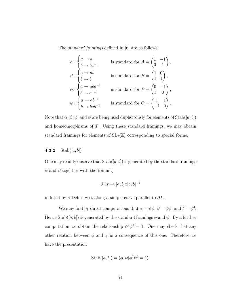
The standard framings defined in [6] are as follows:
α :
a→ a
b→ ba−1is standard for A =
(1 −10 1
),
β :
a→ ab
b→ bis standard for B =
(1 01 1
),
φ :
a→ aba−1
b→ a−1is standard for P =
(0 −11 0
),
ψ :
a→ ab−1
b→ bab−1is standard for Q =
(1 1−1 0
).
Note that α, β, φ, and ψ are being used duplicitously for elements of Stab([a, b])
and homeomorphisms of T . Using these standard framings, we may obtain
standard framings for elements of SL2(Z) corresponding to special forms.
4.3.2 Stab([a, b])
One may readily observe that Stab([a, b]) is generated by the standard framings
α and β together with the framing
δ : x → [a, b]x[a, b]−1
induced by a Dehn twist along a simple curve parallel to ∂T .
We may find by direct computations that α = ψφ, β = φψ, and δ = φ4.
Hence Stab([a, b]) is generated by the standard framings φ and ψ. By a further
computation we obtain the relationship φ2ψ3 = 1. One may check that any
other relation between φ and ψ is a consequence of this one. Therefore we
have the presentation
Stab([a, b]) = 〈φ, ψ|φ2ψ3 = 1〉.
71
Note that φ2 and ψ3 are both in the center of Stab([a, b]). Furthermore,
if j is the transition index between two framings ξ and ζ, then
ξ−1µζµ−1 = φ4j
for some framing µ.
4.3.3 Exponent sums
Definition 4.3.3. Let w be a word on the set of letters Ω, say w =∏k
i=1 xei
i
where xi ∈ Ω and ei ∈ Z. Define the exponent sum of the word w to be
E(w) =∑k
i=1 ei. Define the exponent sum of the letter x for the word w to
be Ex(w) =∑
xi=xei.
Lemma 4.3.1. Let ζ be a framing for Z ∈ SL2(Z), and let ξ be a framing for
X conjugate to Z. Let ω be a word for ζ−1ξ written in φ and ψ. Then
(Eφ(ω), Eψ(ω)) = (4j, 0) mod (2, 3)
where j is the transition index between ζ and ξ.
Proof. First we will show that (Eφ(ω), Eψ(ω)) mod (2, 3) is independent of
choice of the spelling of the word ω.
Let ω and ω′ be two words in φ and ψ representing an element of
Stab([a, b]). The passage between the two words occurs by the following moves:
(i) insertion or deletion of an adjacent pair of a letter and its inverse and
(ii) application of the relation φ2ψ3 = 1.
72
Assume ω and ω′ differ by just one of these moves. Let us examine the effects
upon the exponent sums. Since (i) only introduces or removes cancelling
pairs, it does not change the exponent sums at all. For (ii), let us assume ω ′
is obtained from ω by replacing φ2ψ3 with 1. Then
(Eφ(ω′), Eψ(ω
′)) = (Eφ(ω) − 2, Eψ(ω) − 3) = (Eφ(ω), Eψ(ω)) − (2, 3)
Thus
(Eφ(ω′), Eψ(ω′)) = (Eφ(ω), Eψ(ω)) mod (2, 3)
Let j be the transition index between ζ and ξ. Thus ζ−1µξµ−1 = φ4j
for some framing µ for U ∈ SL2(Z) such that Z−1UXU−1 = I. Let ωζ , ωξ,
and ωµ be words in φ and ψ for ζ, ξ, and µ respectively. Thus we may write
ω−1ζ ωµωξω
−1µ = φ4j.
Therefore since ζ−1µξµ−1 = φ4j , the words ω−1ζ ωµωξω
−1µ and φ4j repre-
sent the same element of Stab([a, b]). Hence it follows that
(Eφ(ω−1ζ ωµωξω
−1µ ), Eψ(ω−1
ζ ωµωξω−1µ )) = (Eφ(φ
4j), Eψ(φ4j)) mod (2, 3)
= (4j, 0) mod (2, 3).
Moreover, notice that Eφ(ωµ) = −Eφ(ω−1µ ) and Eψ(ωµ) = −Eψ(ω−1
µ ), and thus
(Eφ(ω−1ζ ωµωξω
−1µ ), Eψ(ω−1
ζ ωµωξω−1µ )) = (Eφ(ω
−1ζ ωξ), Eψ(ω−1
ζ ωξ)).
Since ω−1ζ ωξ is a word for ζ−1ξ, the conclusion of the lemma follows.
Assume P J . . . Bn(2)An(1) is a special form for an element X of SL2(Z).
This corresponds to an essential twisted surface in the complement of an es-
sential level knot in a once-punctured torus bundle M with characteristic class
73
[X]. Consider the standard framing ξ = φJ . . . βn(2)αn(1) corresponding to the
specific form for X. Assume a framing ζ has been chosen for M , so that
ζ → Z ∈ SL2(Z). Note that Z−1UXU−1 = I for some U ∈ SL2(Z) whereas
ζ−1µξµ−1 = φ4j where µ is any framing for U and j ∈ Z is the transition
index.
Corollary 4.3.2. Continuing with the above notation, let M ∼= S3 −N(K)
for some genus one fibered knot K. Assume Z may be written as a word WZ
in A and B so that the corresponding standard framing is meridional. The
boundary components of C(J ;n(k), . . . , n(2), n(1)) are meridional if and only
if J = 0 and the exponent sum E(WZ) equals∑k
i=1 n(i).
Proof. A boundary component of C(J ;n(k), . . . , n(2), n(1)) intersects a fiber
of M only once if and only if J = 0. The transition index between ξ and
ζ measures how many times the boundary component wraps longitudinally.
Thus the boundary components of C(J ;n(k), . . . , n(2), n(1)) are meridional if
and only if J = 0 and the transition index between ξ and ζ is zero.
Note that the standard framings for A and B are α = ψφ and β = φψ
respectively. Thus Eφ and Eψ are equal on α and β.
Also note that for ω ∈ Stab([a, b]),
(Eφ(ω), Eψ(ω)) = −(Eφ(ω−1), Eψ(ω−1)).
Thus given a word ω written in α and β,
(Eφ(ω), Eψ(ω)) = E(ω)(1, 1) mod (2, 3).
74
Let ωζ be the standard framing for WZ written as a word in α and β.
(Note that ω−1ζ is a word for ζ−1.) Then since ξ = φJ . . . βn(2)αn(1) and J = 0,
let ωξ be the word βn(k) . . . βn(2)αn(1).
Thus we have ζ−1ξ written as the word ω−1ζ ωξ in α and β. Therefore
(Eφ(ω−1ζ ωξ), Eψ(ω−1
ζ ωξ)) = E(ω−1ζ ωξ)(1, 1)
= (E(ω−1ζ ωξ), E(ω−1
ζ ωξ)) mod (2, 3).
Since we need the transition index to be zero, we need
(E(ω−1ζ ωξ), E(ω−1
ζ ωξ)) = (0, 0) mod (2, 3).
In other words, it must be that
(E(ω−1ζ ωξ), E(ω−1
ζ ωξ)) −N(2, 3) = (0, 0)
for some N ∈ Z. This can only happen in the case that E(ω−1ζ ωξ) = 0 and
N = 0. Therefore E(ωζ) = E(ωξ).
Since E(ωζ) = E(WZ) and E(ωξ) =∑k
i=1 n(i), the conclusion of the
corollary follows.
4.4 Algorithms
We now give an algorithm to list all the essential surfaces of type
C(J ;n(k), . . . , n(1)) in the complement of a level knot in a once-punctured
torus bundle.
Algorithm 4.4.1. Let M be a once-punctured torus bundle given by an el-
ement H ∈ SL2(Z). Let L be an essential simple closed curve on the fiber
75

T ×0 of M given by the ordered pair (x, y) ∈ Z2. The following steps give a
procedure to list all essential surfaces of type C(J ;n(k), . . . , n(1)) in M−N(L).
Step 1. Choose a change of basis matrix W ∈ SL2(Z) so that W
(10
)=
(xy
).
Step 2. Let X(N) = (WAN)−1H(WAN).
Step 3. List all N such that X(N) =
(p(N) r(N)q(N) s(N)
)has
|p(N)| < |q(N)|
Step 4. For each N listed in Step 3, obtain the minimal continued fraction ex-
pansions [a1, a2, . . . , ak−1] for p(N)/q(N) such that [a1, a2, . . . , ak−1, ak]
is a continued fraction expansion for r(N)/s(N).
If k is odd, then for either J = +1 or J = −1,
P JAa1Ba2 . . . Aak−2Bak−1Aak = X(N).
If k is even, then for either J = 0 or J = 2,
P JBa1Aa2 . . . Aak−2Bak−1Aak = X(N).
Step 5. For each N in Step 3, list the expressions for X(N) obtained in Step 4.
Step 6. For every expression P JCn(k) . . . Bn(2)An(1) listed in Step 5 (where C = A
or B depending on the parity of k), there is an essential surface of type
C(J ;n(k), . . . , n(1)) in M −N(L).
Proof. Given a change of basis matrix W such that W [a] = [L], all other such
matrices are of the form WAN for some integer N . Proposition 4.1.4 then
76

implies that each expression of X(N) = (WAN)−1H(WAN) as a special form
corresponds to an essential surface in M −N(L) with the type of an essential
twisted surface. Steps 1 and 2 set up X(N), and the remaining steps compute
the special forms for all the X(N).
Lemma 2.3.5 implies that if X(N) =
(p(N) r(N)q(N) s(N)
)has a special form,
then p(N)/q(N) has a MCFE. This then implies that |p(N)/q(N)| < 1 and
hence |p(N)| < |q(N)|. Step 3 lists all such X(N). This is a finite list since
X(N) = A−N (W−1HW )AN and hence q(N) does not depend on N .
Fr each N such that p(N)/q(N) has a MCFE [a1, a2, . . . , ak−1] we may
solve for ak as in Lemma 2.3.6. Then depending on the parity of k, Lemma
2.3.6 gives us the associated special form for X(N). Step 4 lists these special
forms for X(N).
Step 5 collects all the special forms for X(N) for all N . Step 6 then
follows from Proposition 4.1.4.
4.4.1 Computing Framings
Let us continue with the notation of the algorithm above. Given a framing
ζ for M we extend Algorithm 4.4.1 to describe the boundary curves of the
essential surfaces of type C(J ;n(k), . . . , n(1)) in M − N(L) in terms of the
given framing.
Remark 4.4.1. This may be done as a direct computation which has been
previously described in §6.2 of [6]. Lemma 4.3.1 however allows us to simplify
this computation.
77
Algorithm 4.4.2. (Algorithm 4.4.1 Continued: Framing) Let ζ be a framing
for M . For each special form P J . . . Bn(2)An(1) listed in Step 5 of Algorithm
4.4.1, compute the coordinates of the boundary of the associated essential sur-
face as follows:
Step 7. Take ξ to be the standard framing associated to the special form.
Step 8. Write ζ−1ξ as a word ω in the letters φ and ψ.
Step 9. Find j ∈ Z, the transition index, such that
(Eφ(ω), Eψ(ω)) = (4j, 0) mod (2, 3).
In the framing ζ, the boundary components of the essential surface of
type C(J ;n(k), . . . , n(1)) have coordinates 〈1,−j〉, 〈2, 1 − j〉, 〈4, 1 − j〉, or
〈4,−1 − j〉 if J = 0, 2, +1, or −1 respectively.
Proof. In Step 8 we may write ζ−1ξ in terms of φ and ψ by using the normal
form for the structure of Stab([a, b]) as a free product with amalgamation. In
Step 9 we find the transition index via Lemma 4.3.1. Table 1 of [6] lists the
boundary curves for twisted surfaces in terms of their corresponding standard
framings. The transition index tells us how many times around the boundary
of the fiber (the longitude) the boundary of the twisted surface wraps with
respect to the given framing ζ.
4.5 Application to Berge Knots
In this section we will specialize Algorithm 4.4.1 to the case of knots in Kη.
78
Let K be the Left Handed Trefoil, Right Handed Trefoil, or Figure
Eight Knot. Then XK∼= T × I/η where η is α−1 β−1, β α, or α β−1
respectively (c.f. Mη and η−1 of §3.1).
Let L be a knot in Kη. Thus L is a knot in S3 that has a representative
as an essential simple closed curve on the fiber of K.
4.5.1 Passing from XL to XK∪L.
Let S0 be an essential closed (orientable, connected) surface 6∼= S2 in XL.
Assume S0 has been chosen among surfaces in its isotopy class in XL so that
|K ∩ S0| is minimized. Let S = S0 − N(K) ⊂ XK∪L. Note that ∂S is a
collection of meridional curves on ∂N(K).
Lemma 4.5.1. S is essential in XK∪L.
Proof. We must show that S is incompressible, ∂-incompressible, and not
∂-parallel.
Assume S is compressible in XK∪L. Let D be a compressing disk for
S. Since S0 is incompressible, ∂D must bound a disk E ⊂ S0 ⊂ XL. E must
intersect K since otherwise ∂D would bound the disk E in S contradicting that
D is a compressing disk. Let S ′0 = (S0 −N(E)) ∪D. Since XL is irreducible,
S ′0 is isotopic to S0. But then |S0∩K| > |S ′
0∩K| contradicting the minimality
assumption.
Assume S is ∂-parallel. Then S is either a torus parallel to ∂N(L), a
torus parallel to ∂N(K), or an annulus parallel into ∂N(K). If S is parallel to
∂N(L) then S = S0, and so S0 is ∂-parallel in XL. If S is parallel to ∂N(K),
79
then S = S0, and so S is compressible in XL. If S is an annulus parallel into
∂N(K), then since ∂S is a collection of meridional curves, S ∼= S2 in XL.
These all contradict our assumptions on S.
Assume S is ∂-compressible, incompressible, and not ∂-parallel. Since
the boundary components of XK∪L are tori, S must be an annulus. Since ∂S is
a collection of meridional curves, S ∼= S2 in XL contradicting our assumption
otherwise.
4.5.2 Specializing Algorithm 4.4.1
Let K, η, and L be as above. Let H ∈ SL2(Z) be the matrix associated to
η so that H is A−1B−1, BA, or AB−1 if K is the Left Handed Trefoil, Right
Handed Trefoil, or Figure Eight Knot respectively. Note that η is also the
corresponding standard meridional framing.
We specialize Algorithm 4.4.1 and its continuation Algorithm 4.4.2 to
find closed essential surfaces in the complements of knots in Kη.
Algorithm 4.5.2. Let K and η be as above. Let L ∈ Kη be given by the
ordered pair (x, y) ∈ Z2. The following steps give a procedure to list all closed
essential surfaces in XL.
Step 1. Choose a change of basis matrix W ∈ SL2(Z) so that W
(10
)=
(xy
).
Step 2. Let X(N) = (WAN)−1H(WAN).
Step 3. List all N such that X(N) =
(p(N) r(N)q(N) s(N)
)where |p(N)| < |q(N)|.
Step 4. For each N listed in Step 3,
80

• obtain the MCFEs a = [a1, a2, . . . , ak−1] for p(N)/q(N) such that k
is even, and
• find ak such that [a1, a2, . . . , ak−1, ak] is a continued fraction expan-
sion for r(N)/s(N).
Step 5. For each N of Step 3 and for each minimal continued fraction expansion
a = [a1, a2, . . . , ak−1, ak] obtained in Step 4, list those such that
σ(a) = E(H).
Step 6. For each a = [a1, a2, . . . , ak−1, ak] listed in Step 5 there is a closed essen-
tial surface of type C(0; a1, a2, . . . , ak−1, ak) in XL.
Proof. Assume S0 is a closed essential surface in XL. We may isotop S0 to
intersect K minimally. Let S = S0 − N(K). Then by Lemma 4.5.1 S is
essential in XK∪L.
Note that S has meridional boundary on ∂N(K) and is thus transverse
to the induced fibration on ∂N(K). From this and that η (for each of the three
choices) does not fix the isotopy class of any essential curve on T , Proposition
4.2.6 implies S is isotopic to a surface of type C(J ;n(k), . . . , n(1)). Since S
is essential, Proposition 4.1.1 implies that |n(i)| ≥ 2 for i = 2, . . . , k. Since
the components of ∂S are meridional curves, by Corollary 4.3.2 J = 0 and∑k
i=1 n(i) = E(H).
Therefore, to every closed essential surface in XL there is a surface of
type C(0;n(k), . . . , n(1)) in XK∪L such that∑k
i=1 n(i) = E(H). Algorithm
4.4.1 lists all surfaces of type C(J ;n(k), . . . , n(1)) that are essential in XK∪L.
81
The meridional conditions J = 0 and∑k
i=1 n(i) = E(H) are then simple to
check.
We now explain the shortcuts where the algorithm first diverges from
Algorithm 4.4.1 at Step 4.
Since S must have the type of an essential twisted surface with merid-
ional boundary components, J = 0 and hence in Step 4 we take the continued
fraction expansions [a1, a2, . . . , ak−1] where k is even.
At the end of Step 4, we may conclude thatX(N) = P JBa1 . . . Bak−1Aak
where J = 0 or J = 2. The framing condition of Step 5 eliminates the latter
case. If J = 2, this special form has standard framing ξ = φ2βa1 . . . βak−1αak
and since X(N) is conjugate to H which has framing η, Lemma 4.3.1 states
that
(Eφ(ξη−1), Eψ(ξη−1)) = (4j, 0) mod (2, 3).
But since∑ai = E(H),
Eφ(η) = Eψ(η) = Eφ(ξ) − 2 = Eψ(ξ).
Thus
(Eφ(ξη−1), Eψ(ξη−1)) = (−2, 0),
and we get a contradiction. Therefore J = 0.
As in Step 5 of Algorithm 4.4.1, having a special form Ba1 . . . Bak−1Aak
for X(N) yields an essential surface of type C(0; a1, . . . , ak). The conditions
of the current Step 5 imply that the boundary of this surface is meridional.
82

As stated in Step 6, the surface then caps off to a closed surface
C(0; a1, . . . , ak) under the meridional filling of the boundary component of
XK∪L corresponding to K which is essential by Theorem 4.1.2.
4.6 Complements of Essential Surfaces
Let L ∈ Kη be a knot on the fiber of K, the Left or Right Handed Tre-
foil or the Figure Eight Knot, in S3. If S is an essential surface of type
C(0;n(k), . . . , n(1)) in XK∪L then it must be that |n(1)| ≤ 1. If |n(1)| ≥ 2,
then by Proposition 2.5.1 of [6] S would be isotopic to a surface of type
C(0;n(k), . . . , n(1)) that is essential in XK . By the computations of [6] (see
Table 2 of [6]) no such surfaces exist in the complement of K.
Let S0 be a closed essential surface in XL. Thus if S0 is of the type
C(0;n(k), . . . , n(1)) then |n(1)| ≤ 1. Note that S0 must compress under the
trivial filling of XL.
Proposition 4.6.1. Let K, L, and S0 be as above.
• If S0 is of type C(0;n(k), . . . , n(2),±1), then S bounds a handlebody in
S3 and there exists an embedded annulus from S to a longitude of L.
• If S0 is of type C(0;n(k), . . . , n(2), 0), then S does not bound a handle-
body in S3 and there exists an embedded annulus from S to the meridian
of L.
Proof. These annuli are apparent from the pictures Figures 4.4 and 4.5 of the
stacking of the twisted saddle Ca,±1 or Ca,0 upon its predecessor.
83
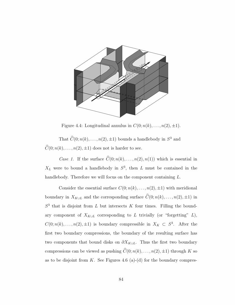
Figure 4.4: Longitudinal annulus in C(0;n(k), . . . , n(2),±1).
That C(0;n(k), . . . , n(2),±1) bounds a handlebody in S3 and
C(0;n(k), . . . , n(2),±1) does not is harder to see.
Case 1. If the surface C(0;n(k), . . . , n(2), n(1)) which is essential in
XL were to bound a handlebody in S3, then L must be contained in the
handlebody. Therefore we will focus on the component containing L.
Consider the essential surface C(0;n(k), . . . , n(2),±1) with meridional
boundary in XK∪L and the corresponding surface C(0;n(k), . . . , n(2),±1) in
S3 that is disjoint from L but intersects K four times. Filling the bound-
ary component of XK∪L corresponding to L trivially (or “forgetting” L),
C(0;n(k), . . . , n(2),±1) is boundary compressible in XK ⊂ S3. After the
first two boundary compressions, the boundary of the resulting surface has
two components that bound disks on ∂XK∪L. Thus the first two boundary
compressions can be viewed as pushing C(0;n(k), . . . , n(2),±1) through K so
as to be disjoint from K. See Figures 4.6 (a)-(d) for the boundary compres-
84
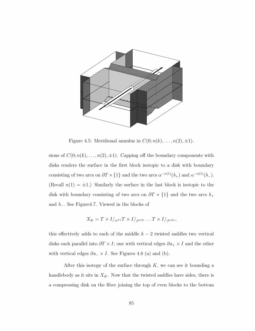
Figure 4.5: Meridional annulus in C(0;n(k), . . . , n(2),±1).
sions of C(0;n(k), . . . , n(2),±1). Capping off the boundary components with
disks renders the surface in the first block isotopic to a disk with boundary
consisting of two arcs on ∂T ×1 and the two arcs α−n(1)(b+) and α−n(1)(b−).
(Recall n(1) = ±1.) Similarly the surface in the last block is isotopic to the
disk with boundary consisting of two arcs on ∂T × 1 and the two arcs b+
and b−. See Figure4.7. Viewed in the blocks of
XK = T × I/α±1T × I/βn(2) . . . T × I/βn(k) ,
this effectively adds to each of the middle k − 2 twisted saddles two vertical
disks each parallel into ∂T × I; one with vertical edges ∂a+ × I and the other
with vertical edges ∂a− × I. See Figures 4.8 (a) and (b).
After this isotopy of the surface through K, we can see it bounding a
handlebody as it sits in XK. Now that the twisted saddles have sides, there is
a compressing disk on the fiber joining the top of even blocks to the bottom
85

(a) One ∂-compressing disk. (b) Both ∂-compressing disks.
(c) After two ∂-compressions. (d) After an isotopy
Figure 4.6: Boundary compressions of C(0;n(k), . . . , n(2),±1).
of odd blocks, i.e. the fiber T × 1 of the ith block for 2 ≤ i ≤ k − 2 even.
This compressing disk is visible in T ×1 of Figure 4.8 (a) and in T ×0 of
Figure 4.8 (b).
Compressing the surface along these 12k− 1 disks separates the surface
into 12k tori. There is one torus in each pair of an odd numbered block with
its successive even numbered block. These tori bound solid tori. Undoing the
12k − 1 compressions by attaching 1-handles to these solid tori and reversing
the isotopies, we conclude that C(0;n(k), . . . , n(2),±1) bounds a handlebody.
Case 2. Consider the surface C(0;n(k), . . . , n(2), 0) ⊂ S3 and its corre-
sponding surface C(0;n(k), . . . , n(2), 0) ⊂ XK in the complement of L. Let H
86

Figure 4.7: Adding sides to the first and last block.
(a) (b)
Figure 4.8: Adding sides to twisted saddles.
be the SL2(Z) monodromy of the punctured torus bundle XK . As in Remark
4.1.1, H is conjugate to Bn(k)An(k−1) . . . An(3)Bn(2)A0. Therefore
[H] = [Bn(k)An(k−1) . . . An(3)Bn(2)A0]
= [An(k−1) . . . An(3)Bn(2)A0Bn(k)]
= [An(k−1) . . . An(3)Bn(2)+n(k)]
= [P−1An(k−1) . . . An(3)Bn(2)+n(k)P ]
= [P−1PBn(k−1) . . . Bn(3)An(2)+n(k)] = [Bn(k−1) . . . Bn(3)An(2)+n(k)].
Since |n(i)| ≥ 2 for i = 3, . . . , k− 1 and the exponent sum is no different, this
corresponds to another essential surface C(0;n(k − 1), . . . , n(3), n(2) + n(k))
87
with meridional boundary in XK in the complement of another level knot L′.
This surface C(0;n(k − 1), . . . , n(3), n(2) + n(k)) is obtained by compressing
along the “obvious” compressing disk for C(0;n(k), . . . , n(2), 0) forgetting L.
Note that L′ must be contained in the component of XK − N(C(0;n(k −
1), . . . , n(3), n(2) + n(k))) that does not come from the component of XK −
N(C(0;n(k), . . . , n(2), 0)) that contained L. Also note that n(2) + n(k) = ±1
or 0.
Let us assume that C(0;n(k), . . . , n(2), 0) bounds a handlebody V to
the side containing L in S3. The other side must be incompressible. Note that
C(0;n(k), . . . , n(2), 0) 6∼= S2 since there is a properly embedded separating
disk (the compressing disk) that L intersects once. The compression yielding
C(0;n(k−1), . . . , n(3), n(2)+n(k)) compresses V along a nonseparating curve
to yield another handlebody V ′ which does not contain the new level knot L′.
This contradicts that C(0;n(k − 1), . . . , n(3), n(2) + n(k)) is essential in XL′
unless C(0;n(k − 1), . . . , n(3), n(2) + n(k)) ∼= S2.
If C(0;n(k−1), . . . , n(3), n(2)+n(k)) ∼= S2, then k = 4 so that the sur-
face is C(0;n(3), n(2)+n(4)). However, one may check that there are no special
forms Bn′(2)An′(1) where |n′(2)| ≥ 2 and |n′(1)| ≤ 1 that are conjugate to H.
(In fact one may check that there are no special forms Bn′(4)An′(3)Bn′(2)An
′(1)
where |n′(i)| ≥ 2 for i = 2, 3, 4 and |n′(1)| ≤ 1 that are conjugate to H either.)
88

4.7 Examples
Let K be the Left Handed Trefoil. Let η = α−1 β−1 and H = A−1B−1.
Here we give some examples of the application of Algorithm 4.5.2 to knots in
Kη = Kα−1β−1 , the knots on the fiber of the Left Handed Trefoil.
4.7.1 Genus 2 surfaces and the knots 1+2z4z
∈ Kη.
Let L ∈ Kη be a knot with slope 1+2z4z
such that z ≥ 3 is an integer. We apply
Algorithm 4.5.2.
Step 1. Choose W =
(1 + 2z −z
4z 1 − 2z
).
Step 2. X(N) = (WAN)−1H(WAN).
X(N) =(
3z − 6z2 + (1 + 12z2)N 1 − 3z + 3z2 − (1 − 6z + 12z2)N + (1 + 12z2)N2
−(1 + 12z2) 1 − 3z + 6z2 − (1 + 12z2)N
)
Step 3. q(N) = −(1 + 12z2) and p(N) = 3z − 6z2 + (1 + 12z2)N . Therefore
|p(N)| < |q(N)| if N = 0 or N = −1.
Step 4. Recall that we are assuming z ≥ 3.
(N = 0.) p(0)/q(0) = −3z+6z2
1+12z2has SCFE [2, 1 − z, 2,−1, z − 1,−2]. We have
the following MCFEs and determine their corresponding ak:
• [2,−z,−2,−2, z, 2], ak = +1
• [2,−z,−2,−3,−2, . . . ,−2︸ ︷︷ ︸z−2
,−3], ak = 0
• [2, 1 − z, 3, z,−2], ak = 0
• [2, 1 − z, 3, z + 1, 2], ak = +1
89

• [3, 2, . . . , 2︸ ︷︷ ︸z−2
, 3,−2, . . . ,−2︸ ︷︷ ︸z−1
,−3], ak = 0
• [3, 2, . . . , 2︸ ︷︷ ︸z−2
, 4, z,−2], ak = 0
• [3, 2, . . . , 2︸ ︷︷ ︸z−2
, 4, z + 1, 2], ak = +1
(N = −1). p(−1)/q(−1) = −1−3z−6z2
1+12z2has SCFE [−1, 1, 1 − z, 2,−1, z − 1,−2].
We have the following MCFEs and determine their corresponding
ak:
• [−2,−z − 1,−2,−3,−2, . . . ,−2︸ ︷︷ ︸z−2
,−3], ak = −1
• [−2,−z − 1,−2,−2, z, 2], ak = 0
• [−2,−z − 1,−2,−2, z − 1,−2], ak = −1
• [−2,−z, 2,−2, . . . ,−2︸ ︷︷ ︸z−1
,−3], ak = −1
• [−2,−z, 3, z + 1, 2], ak = 0
• [−2,−z, 3, z,−2], ak = −1
Note that some of these MCFEs have k odd.
Step 5. Since E(H) = E(A−1B−1) = −2, we get just one list a1, . . . , ak−1, ak
such that k is even and∑k
i=1 ai = −2:
−2,−z, 3, z,−2,−1
Step 6. The knot L given by (1 + 2z, 4z) for z ≥ 3 contains the closed essential
surface C(0;−2,−z, 3, z,−2,−1) in its complement. Furthermore, this
is the only one.
One can actually show that a knot in Kη with slope 1+2z4z
for |z| ≥ 2
has the surface C(0;−2,−z, 3, z,−2,−1) as the only closed essential surface
90
in its complement. Moreover, one can show that if a knot in Kη has a closed
essential genus 2 surface in its complement, then it is one of these knots. A
similar result is also true for the knots on the fiber of the Figure Eight Knot.
4.7.2 Higher genus surfaces.
By doing the reverse of the compression in Case 2 of Proposition 4.6.1 we can
construct many more knots with close essential surfaces in their complements.
Using the above example as a model, we obtained the closed essential surface
C(0;−2,−z, 3, z,−2,−1) in the complement of the knot 1+2z4z
∈ Kη. Thus
(A−NW−1)A−1B−1(WAN ) = B−2A−zB3AzB−2A−1
= B−2A−zB3AzB−2Az′−1B0A−z′
A−z′(A−NW−1)A−1B−1(WAN )Az′ = A−z′B−2A−zB3AzB−2Az′−1B0
P−1A−z′(A−NW−1)A−1B−1(WAN )Az′P = P−1A−z′B−2A−zB3AzB−2Az′−1B0P
(P−1A−z′A−NW−1)A−1B−1(WANAz′P ) = B−z′A−2B−zA3BzA−2Bz′−1A0.
Since W =
(1 + 2z −z
4z 1 − 2z
)and N = 0,
WANAz′
P =
(−z − z′ − 2zz′ −1 − 2z1 − 2z − 4zz′ −4z
).
Hence if |z′| ≥ 2 and |z′−1| ≥ 2 (and |z| ≥ 2), the knot z+z′+2zz′
−1+2z+4zz′∈ Kη has in
its complement the closed essential surface C(0;−z′,−2,−z, 3, z,−2, z′ − 1, 0)
of genus 3.
This process may be repeated to construct knots in Kη whose comple-
ments contain a closed essential surface of genus g for any g ≥ 2. There are
closed essential surfaces in the complements of knots in Kη, however, that are
not constructed in this manner.
91

4.7.3 A small knot
As seen in the following chapter there are many small knots in Kη. Here we
give an example of the algorithm applied to a simple knot (which is not a torus
knot) to show it is small.
Let L ∈ Kη be the knot −32∈ Kη. We apply Algorithm 4.5.2.
Step 1. Choose W =
(−3 12 −1
).
Step 2. X(N) = (WAN)−1H(WAN).
X(N) =
(−7 − 19N 3 + 15N + 19N 2
−19 8 + 19N
)
Step 3. q(N) = −19 and p(N) = −7− 19N . Therefore |p(N)| < |q(N)| if N = 0
or N = −1.
Step 4.
(N = 0.) p(0)/q(0) = 719
has SCFE [2,−1, 2,−2] and two MCFEs of odd
length: [3, 4, 2] and [3, 3,−2].
For [3, 4, 2]:
[3, 4] = (r(0) + p(0)a4)/(s(0) + q(0)a4)
⇒4
13=
3 − 7a4
8 − 19a4
=⇒ a4 = 1
For [3, 3,−2]
[3, 3] = (r(0) + p(0)a4)/(s(0) + q(0)a4)
⇒3
8=
3 − 7a4
8 − 19a4
=⇒ a4 = 0
92

(N = −1). p(−1)/q(−1) = − 1219
has SCFE [−1, 1,−1, 2,−2] and no MCFE of
odd length.
Step 5. We have two lists:
3, 4, 2, 1 and 3, 3,−2, 0.
Their sums are 10 and 4 respectively. Neither equals E(H) = −2.
Step 6. Since we have no lists satisfying all the criteria, there are no closed
essential surfaces in the complement of L.
93
Chapter 5
Volumes and Surfaces
Both estimates on volumes of knots L in K and the computation of closed
essential surfaces in the complements of such knots are related to continued
fraction expansions of rational numbers. Similar relationships between con-
tinued fraction expansions and essential surfaces have appeared in [10] and
[7].
In this chapter we apply Algorithm 4.4.1 to knots L ∈ Kη in general.
Given the slope of L, we exhibit an equation in terms of the SCFE for the slope
whose solutions correspond to all closed essential surfaces in the complement
of L. Because estimates on vol(L) (if L is hyperbolic) may be obtained from
continued fraction expansions for its slope, we are able to give lower bounds
for the genera of closed essential surfaces in XL in terms of lower bounds
on vol(L). Furthermore we can construct knots in Kη with arbitrarily many
distinct closed essential surfaces in their complements. Contrasting this, we
can use similar techniques to construct small knots in Kη and even show that
Kη contains small knots of arbitrarily large volume.
Throughout this chapter we work with η = α−1 β−1, hence Kη are
the knots that lie on the fiber of the Left Handed Trefoil. Similar results can
94
be obtained for both the families of knots that lie on the fiber of the Right
Handed Trefoil and those that lie on the Figure Eight Knot.
5.1 General Setup.
We apply Algorithm 4.5.2 to the knots L ∈ Kη in general. Throughout this
section when N = ±1, the symbol ± agrees with the sign of N .
Let [b] = [b1, b2, . . . , bk] be the SCFE for the slope xy
of the knot L.
Recall that only b1 may be 0 and consecutive coefficients do not have the same
sign. We also assume xy6= 0, ±1, or 1
0since these slopes all correspond to the
unknot.
Theorem 5.1.1. For L as above, every closed essential surface in its comple-
ment corresponds to a solution of one of the following equations:
1. If b1 6= 0 or 1,
0 =∑
i∈I
−bi +∑
j∈J
bj +
0 if 1 ∈ I
−1 otherwise
where I and J are subsets of 1, . . . , k each not containing consecutive
integers and 1 6∈ I ∩ J .
2. If b1 = 0 and b2 6= −1,
0 =∑
i∈I
−bi +∑
j∈J
bj +
0 if 2 ∈ J
−1 otherwise
where I and J are subsets of 2, . . . , k each not containing consecutive
integers and 2 6∈ I ∩ J .
95

3. If b1 = 0 and b2 = −1,
0 =∑
i∈I
−bi +∑
j∈J
bj +
0 if 3 ∈ J
−1 otherwise
where I and J are subsets of 3, . . . , k each not containing consecutive
integers and 3 6∈ I ∩ J .
4. If b1 = 1,
0 =∑
i∈I
−bi +∑
j∈J
bj +
0 if 2 ∈ I
−1 otherwise
where I and J are subsets of 2, . . . , k each not containing consecutive
integers and 2 6∈ I ∩ J .
For the resulting surface to be essential we have the extra following
conditions on I and J .
1. If b1 6= 0 or 1, then if bl = ±1 for l ≥ 2, then l− 1, l, l+ 1∩ I 6= ∅ and
l − 1, l, l + 1 ∩ J 6= ∅. If b1 = −1 then either 1 ∈ I or 1, 2 ∩ J 6= ∅.
If b1 = 2 then either 1 ∈ J or 1, 2 ∩ I 6= ∅.
2. If b1 = 0 and b2 6= −1, then if bl = ±1 for l ≥ 3, then l−1, l, l+1∩I 6= ∅
and l−1, l, l+1∩J 6= ∅. If b2 = −2 then either 2 ∈ I or 2, 3∩J 6= ∅.
If b2 = 1 then either 2 ∈ J or 2, 3 ∩ I 6= ∅.
3. If b1 = 0 and b2 = −1, then if bl = ±1 for l ≥ 4, then l−1, l, l+1∩I 6= ∅
and l− 1, l, l+1∩J 6= ∅. If b3 = 1 then either 3 ∈ J or 3, 4∩ I 6= ∅.
4. If b1 = 1, then if bl = ±1 for l ≥ 3, then l − 1, l, l + 1 ∩ I 6= ∅ and
l − 1, l, l + 1 ∩ J 6= ∅. If b2 = −1 then either 2 ∈ I or 2, 3 ∩ J 6= ∅.
96

Remark 5.1.1. Cases 2 − 4 and the extra conditions on the sets I and J are
not needed if [b] is a MCFE as well as a SCFE with b1 6= 2.
Proof. Set W =
(x ty u
)∈ SL2(Z) where
x
y= [b1, b2, . . . , bk] and
t
u= [b1, b2, . . . , bk−1].
Then by Lemma 2.3.5 W may be written as
±Bb1Ab2 . . . Bbk or ± BABAb1Bb2 . . . Bbk
depending on the parity of k.
Let
X(N) = (WAN)−1A−1B−1(WAN) =
(p(N) q(N)r(N) s(N)
)AN
for N ∈ Z. Then X(N) may be written as
(±A−NB−bk . . . A−b2B−b1)A−1B−1(±Bb1Ab2 . . . BbkAN)
= A−NB−bk . . . A−b2B−b1A−1Bb1−1Ab2 . . . BbkAN
or
(±A−NB−bk . . . B−b2A−b1B−1A−1B−1)A−1B−1(±B1A1B1Ab1Bb2 . . . BbkAN)
= A−NB−bk . . . B−b2A−b1B−1Ab1−1Bb2 . . . BbkAN
depending on the parity of k. In either case, note that
p(N)/q(N) = [0,−N,−bk, . . . ,−b2,−b1,−1, b1 − 1, b2, . . . , bk].
Define [x(N)] = [0,−N,−bk, . . . ,−b2,−b1,−1, b1 − 1, b2, . . . , bk].
97

According to Algorithm 4.5.2 for every MCFE [xm] = [a1, a2, . . . , al] of
p(N)/q(N) of odd length such that N ′ = −2 − σ(xm) and [a1, a2, . . . , al, N′]
is a continued fraction expansion for r(N)/s(N) for some N there is a closed
essential surface in the complement of L. Since every MCFE of a rational
number is derived from its SCFE (as noted in §2.3.1), we need to obtain the
SCFE [xs(N)] for p(N)/q(N). We determine the SCFE in §5.1.1 and the
MCFEs corresponding to essential surfaces in §5.1.2.
5.1.1 SCFE for p(N)/q(N).
First recall that if p(N)/q(N) is to have a MCFE then its absolute value must
be less than 1. Since p(N)/q(N) = [x(N)],
p(N)/q(N) =1
0 −1
−N − [b′]
= N + [b′]
where [b′] = [−bk, . . . ,−b2,−b1,−1, b1 − 1, b2, . . . , bk].
Lemma 5.1.2. |[b′]| < 1 and sign([b′]) = sign(−bk).
Proof. We exhibit the SCFE for [b′]. The first coefficient will be nonzero and
hence imply the conclusion of the lemma.
By move (CF 1),
[b′] 7→ [b′1] = [−bk, . . . ,−b2,−b1 + 1, b1, b2, . . . , bk].
This is a SCFE unless b1 = 0 or 1.
Case b1 = 0. By move (CF 1)
[b′1] = [−bk, . . . ,−b2, 1, 0, b2, . . . , bk]
7→ [−bk, . . . ,−b3,−b2, b2 + 1, b3, . . . , bk] = [b′2]
98

which is a SCFE unless b2 = −1 or 0. Since [b] is a SCFE, b2 cannot be 0.
Furthermore k > 1 since [b] 6= 0.
If b2 = −1 then by move (CF 1)
[b′2] = [−bk, . . . ,−b3, 1, 0, b3, . . . , bk]
7→ [−bk, . . . ,−b4,−b3, b3 + 1, b4, . . . , bk] = [b′3]
which is a SCFE unless b3 = −1 or 0. Since [b] is a SCFE and b2 = −1 neither
of these two situations can occur. Furthermore if k = 2 then [b] = [0,−1] = 1
contrary to our assumption on xy.
Case b1 = 1. By move (CF 1)
[b′1] = [−bk, . . . ,−b2, 0, 1, b2, . . . , bk]
7→ [−bk, . . . ,−b3,−b2 + 1, b2, b3, . . . , bk] = [b′4]
which is a SCFE unless b2 = 0 or 1. Since [b] is a SCFE and b1 = 1 neither of
these two situations can occur. Furthermore if k = 1 then [b] = 1 contrary to
our assumption on xy.
Each of [b′i] for i = 1, 2, 3, 4 has nonzero leading coefficient. One of
these is the SCFE for [b′]. Therefore by Lemma 2.3.1, |[b′]| < 1 and sign([b′]) =
sign(−bk).
Corollary 5.1.3. If p(N)/q(N) has a MCFE then either N = 0 or N = ±1
such that sign(N) = sign(bk).
Proof. A rational number has a MCFE only if its absolute value is less than
1. Since p(N)/q(N) = [0, N, b′] = N + [b′] and by Lemma 5.1.2 |[b′]| < 1,
99
|p(N)/q(N)| < 1 if and only if either N = 0 or N = ±1 such that sign(N) 6=
sign([b′]). However, sign([b′]) = sign(−bk) = − sign(bk).
Remark 5.1.2. Corollary 5.1.3 shows that we really only need to consider two
values of N in Algorithm 4.5.2.
We now find the SCFE [xs(N)] for p(N)/q(N).
If N = 0, then for one of i = 1, 2, 3, or 4.
p(0)/q(0) = [x(0)] = [0, 0, b′i] = [b′i]
is the SCFE.
If N = ±1, then for i = 1, 2, 3, or 4 such that [b′i] is a SCFE
p(±1)/q(±1) = [x(±1)] = [0,∓1, b′i] = [0,∓1,−bk, . . . , bk]
7→ [±1,−bk ± 1, . . . , bk] = [b′′i ]
by move (CF 1). This is a SCFE unless bk = 0 or ±1. Since [b′i] is a SCFE,
|bk| ≥ 2. Therefore [b′′i ] is the SCFE.
Notice that the move (CF 1’) is never used in obtaining [xs(N)] from
[x(N)]. Hence their last two partial sums are equal. Furthermore, as a conse-
quence of Lemma 2.3.6 there exists an Ns such that [x(N), N ] = [xs(N), Ns].
Therefore by Lemma 2.3.2, Ns = N ′.
There are two extra “degenerate” cases to consider for the SCFE of
p(N)/q(N).
If n = 2, i = 4 (so b1 = 1), and N = 1, then
[b′4] = [1,−b2 + 1 + 1, b2] = [1,−b2 + 2, b2]
100

is a SCFE unless b2 = 0, 1, or 2. These cannot occur since b1 = 1 and [b] is a
SCFE.
If n = 1, i = 1, and N = 1, then
[b′1] = [1,−b1 + 1 + 1, b1] = [1,−b1 + 2, b1]
is a SCFE unless b1 = 0, 1, or 2. By our assumption on xy, b1 6= 0 or 1.
However, b1 may equal 2 in which case xy
= 12. This slope corresponds to the
unknot.
Therefore we obtain:
Lemma 5.1.4. For N = 0 or ±1, p(N)/q(N) has SCFE [xs(N)] where
xs(0) = b′i and xs(±1) = b′′i for some i ∈ 1, 2, 3, 4. Furthermore r(N)/s(N)
has the continued fraction expansion [xs(N), N ].
5.1.2 MCFEs and Surfaces.
Given the SCFE [xs(N)] for p(N)/q(N), we determine every MCFE [xm] of
odd length and N ′ such that both r(N)/s(N) = [xm, N′] and σ(xm) + N ′ =
σ(x(N)) +N .
For such an [xm] andN ′, since [xs(N), N ] = r(N)/s(N) by Lemma 5.1.4,
Lemma 2.3.4 implies σ(xm) − σ(x(N)) = N −N ′ =
0
sign(bk).
We have four cases for the four different possibilities of the SCFE
[xs(N)] depending on [b] each of which has the two cases ofN = 0 andN = ±1.
See Lemma 5.1.4.
1. If b1 6= 0, 1 then [xs(0)] = [b′1] and [xs(±1)] = [b′′1].
101
2. If b1 = 0 and b2 6= −1 then [xs(0)] = [b′2] and [xs(±1)] = [b′′2].
3. If b1 = 0 and b2 = −1 then [xs(0)] = [b′3] and [xs(±1)] = [b′′3].
4. If b1 = 1 then [xs(0)] = [b′4] and [xs(±1)] = [b′′4].
Case 1. b1 6= 0, 1
The SCFEs for p(N)/q(N) for N = 0,±1 are
[xs(0)] = [b′1] = [−bk, . . . ,−b2,−b1 + 1, b1, b2, . . . , bk]
and
[xs(±1)] = [b′′1] = [±1,−bk ± 1, . . . ,−b2,−b1 + 1, b1, b2, . . . , bk].
Subcase N = 0.
Assume [xm] is a MCFE for p(0)/q(0). Then it is obtained from
[xs(0)] = [b′1] by applying moves (M) and (M’) to nonadjacent coefficients
of [b′1]. (C.f. §2.3.1.) In particular, if a coefficient of [b′1], then (M) or (M’)
must be applied to it or an adjacent coefficient to make the all the resulting
coefficients of [xm] not ±1.
The difference of coefficient sums between [xm] and [b′1] is
σ(xm) − σ(b′1) =∑
i∈I
−3(−bi) +
−3(1) if 1 ∈ I
0 otherwise+∑
j∈J
−3(bj)
+
sign(bk) if k ∈ J
0 otherwise
= −3
(∑
i∈I
−bi +
1 if 1 ∈ I
0 otherwise+∑
j∈J
bj
)
+
sign(bk) if k ∈ J
0 otherwise
102

where I ⊂ 1, . . . , k − 1 and J ⊂ 1, . . . , k each not containing consecutive
integers and 1 6∈ I ∩ J . If k ∈ J , then we take sign(bk) since we need +1
if bk > 0 and −1 if bk < 0. The indexing sets I and J correspond to the
coefficients to which the moves (M) and (M’) are applied.
Since σ(xm) − σ(x(0)) =
0
sign(bk)and
σ(xs(0)) − σ(x(0)) = σ(b′1) − σ(x(0)) = 1 −−2 = +3,
then
0sign(bk)
= σ(xm) − σ(x(0))
= σ(xm) − σ(b′1) + σ(b′1) − σ(x(N))
= −3
(∑
i∈I
−bi +
1 if 1 ∈ I
0 otherwise+∑
j∈J
bj
)
+
sign(bk) if k ∈ J
0 otherwise+ 3
= −3
(∑
i∈I
−bi +
1 if 1 ∈ I
0 otherwise+∑
j∈J
bj − 1
)
+
sign(bk) if k ∈ J
0 otherwise
= −3
(∑
i∈I
−bi +∑
j∈J
bj +
0 if 1 ∈ I
−1 otherwise
)
+
sign(bk) if k ∈ J
0 otherwise.
If k ∈ J then
0sign(bk)
= −3
(∑
i∈I
−bi +∑
j∈J
bj +
0 if 1 ∈ I
−1 otherwise
)+ sign(bk)
103
which implies we must take σ(xm) − σ(x(0)) = sign(bk). Thus if k ∈ J , then
N ′ = N − sign(bk) = − sign(bk).
If k 6∈ J , then similarly we must take which implies we must take
σ(xm) − σ(x(0)) = 0. Thus if k 6∈ J , then N ′ = N = 0.
In either situation,
0 = −3
(∑
i∈I
−bi +∑
j∈J
bj +
0 if 1 ∈ I
−1 otherwise
),
and hence
0 =∑
i∈I
−bi +∑
j∈J
bj +
0 if 1 ∈ I
−1 otherwise.
Subcase N = ±1.
Assume xm is a MCFE for p(±1)/q(±1). Then it is obtained from
[xs(±1)] = [b′′1] by applying moves (M) and (M’) to nonadjacent coefficients of
[xs(0)]. (C.f. §2.3.1.) Again, if a coefficient of [b′′1] is ±1, then move (M) or
(M’) must be applied to it or an adjacent coefficient.
Then the difference of coefficient sums is
σ(xm)− σ(b′′1) = −3(±1) +∑
i∈I
−3(−bi) +
−3(1) if 1 ∈ I
0 otherwise+∑
j∈J
−3(bj)
+
sign(bk) if k ∈ J
0 otherwise
= −3
(±1 +
∑
i∈I
−bi +
1 if 1 ∈ I
0 otherwise+∑
j∈J
bj
)
+
sign(bk) if k ∈ J
0 otherwise
where I ⊂ 1, . . . , k−2, k and J ⊂ 1, . . . , k each not containing consecutive
integers, k ∈ I, and 1 6∈ I ∩ J . Note that we must apply move (M) to the
104
second coefficient −bk ± 1 in [b′′1] to account for the leading coefficient of ±1,
hence k ∈ I. Also if k ∈ J , then we take sign(bk) since we need +1 if bk > 0
and −1 if bk < 0. As noted in the previous case, the indexing sets I and J
correspond to the coefficients to which the moves (M) and (M’) are applied.
Since σ(xm) − σ(x(±1)) =
0
sign(bk)and
σ(xs(±1)) − σ(x(±1)) = σ(b′′1) − σ(x(±1))
= (±2 + 1) − (∓1 + −2) = ±3 + 3
then
0sign(bk)
= σ(xm) − σ(x(±1))
= σ(xm) − σ(b′′1 + σ(b′′1) − σ(x(±1))
= −3
(±1 +
∑
i∈I
−bi +
1 if 1 ∈ I
0 otherwise+∑
j∈J
bj
)
+
− sign(bk) if k ∈ J
0 otherwise± 3 + 3
= −3
(±1 +
∑
i∈I
−bi +
1 if 1 ∈ I
0 otherwise+∑
j∈J
bj ∓ 1 − 1
)
+
sign(bk) if k ∈ J
0 otherwise
= −3
(∑
i∈I
−bi +∑
j∈J
bj +
0 if 1 ∈ I
−1 otherwise
)
+
sign(bk) if k ∈ J
0 otherwise.
If k ∈ J then
0sign(bk)
= −3
(∑
i∈I
−bi +∑
j∈J
bj +
0 if 1 ∈ I
−1 otherwise
)+ sign(bk)
105
which implies we must take σ(xm) − σ(x(0)) = sign(bk). Thus if k ∈ J , then
N ′ = N − sign(bk) = ±1 − sign(bk) = 0 since sign(bk) = N = ±1.
If k 6∈ J , then similarly we must take which implies we must take
σ(xm) − σ(x(0)) = 0. Thus N ′ = N = ±1.
In either situation,
0 = −3
(∑
i∈I
−bi +∑
j∈J
bj +
0 if 1 ∈ I
−1 otherwise
)
and hence
0 =∑
i∈I
−bi +∑
j∈J
bj +
0 if 1 ∈ I
−1 otherwise.
The only difference between the outcomes of these two subcases is in
the indexing set I. If N = 0 then I ⊂ 1, . . . , k−1 containing no consecutive
integers. If N = ±1 then I ⊂ 1, . . . , k−2, k containing k and no consecutive
integers. (Notice that N = 0 if k 6∈ I and N = ±1 = sign(bk) if k ∈ I.) These
two conditions can be consolidated by taking I ⊂ 1, . . . , k containing no
consecutive integers. Therefore a solution to the equation
0 =∑
i∈I
−bi +∑
j∈J
bj +
0 if 1 ∈ I
−1 otherwise(*)
where I and J are subsets of 1, . . . , k each not containing consecutive integers
and 1 6∈ I ∩ J corresponds to an N = 0 or ±1, a continued fraction [xm] =
p(N)/q(N), and an N ′ such that both [xm, N′] = r(N)/s(N) and σ(xm)+N ′ =
σ(x(N)) +N . The continued fraction [xm] will be minimal only if moves (M)
or (M’) are applied to coefficients ±1 of [xs(N)] or their neighbors.
A priori, such an [xm] might not be of odd length. Following the method
106
for calculating coefficient sums, the length of [xm] is given by
length(xm) − length(xs(N)) =∑
i∈I
(| − bi| − 2) +∑
j∈J
(|bj| − 2)
+
0 if 1 ∈ I
−1 otherwise+
N if k ∈ I
0 otherwise.
Because [xs(N)] is [b′1] when k 6∈ I and [b′′1] when k ∈ I,
length(xs(N)) =
2k if k 6∈ I
2k + 1 if k ∈ I.
Viewing this mod 2, [xm] has odd length if and only if
1 −
0 if k 6∈ I
1 if k ∈ I.=∑
i∈I
−bi +∑
j∈J
bj
+
0 if 1 ∈ I
−1 otherwise+
1 if k ∈ I
0 otherwisemod 2.
Therefore
0 =∑
i∈I
−bi +∑
j∈J
bj +
0 if 1 ∈ I
−1 otherwisemod 2.
Hence the odd length of [xm] is implied by the solution to equation (*). The
conclusion of the theorem in this case follows.
Cases 2 - 4. These last three cases follow much the same via the appropriate
substitutions of [. . . ,−b2,−b1 + 1, b1, b2, . . . ] by [. . . ,−b3,−b2, b2 + 1, b3, . . . ],
[. . . ,−b4,−b3, b3 + 1, b4, . . . ], and [. . . ,−b3,−b2 + 1, b2, b3, . . . ].
The conclusion of Theorem 5.1.1 then follows.
107
5.2 Corollaries.
5.2.1 Genera of Surfaces.
Corollary 5.2.1. If L ∈ Kη is a hyperbolic knot with vol(L) > vol(L(2n +
1), η) > (2n + 1) · v, then XL contains no closed essential surfaces of genus
less than 12(n− 1).
Proof. Assume L ∈ Kη has volume greater than vol(L(2n+ 1), η). Then since
volume decreases under surgery, L cannot be written as surgery on the link
L(2n+ 1, η). Thus if L has slope xy, then any continued fraction expansion for
xy
must have length greater than n.
Let [b] = [b1, b2, . . . , bk] be the SCFE for xy. Note that k > n. Construct
[xs(N)] as in Lemma 5.1.4.
Since [b] has length k, the length of [xs(N)] must be at least 2k − 2,
the length of [b′4].
Since the genus of a closed essential surface is related to the length
of the associated MCFE of p(N)/q(N), we need to see how much shorter a
MCFE can be that the SCFE from which it is obtained.
Recall that any MCFE may be obtained from the corresponding SCFE
by the moves (M 1) and (M 1’) on non-adjacent coefficients of the SCFE. Since
length only decreases under these moves applied to a coefficient of ±1, each of
which decreases the length by 1, the length of a MCFE must be at least half
the length of its corresponding SCFE. Generically, however, the length will
increase.
108

Therefore the length of a MCFE for p(N)/q(N) must be at least 12(2k−
2) and hence greater than k − 1. Since k > n, the length of a MCFE for
p(N)/q(N) is greater than n−1. If a MCFE [xm(N)] for p(N)/q(N) of length
k′ corresponds to a twisted surface with meridional boundary, then the genus
of the closed essential surface is 12(k′+1)−1. Since k′ ≥ k, the genus of a closed
essential surface in the complement of L must be greater than 12(n− 1) − 1.
Corollary 5.2.2. There exist knots in Kη with arbitrarily many distinct closed
essential surfaces in their complements.
Proof. Let [b] = [b1, . . . , bk] be the SCFE of the slope of a knot K0 ∈ Kη
with a closed essential surface in its complement such that b1 6= 0 or 1. By
Theorem 5.1.1 there are subsets I0 and J0 of 1, . . . , k such that
0 =∑
i∈I0
−bi +∑
j∈J0
+
0 if 1 ∈ I
−1 otherwise.
For each integer r ≥ 2, let [ar] = [ak+1, ak+2, . . . , ak+r] be a SCFE and a MCFE
such that sign(ak+1) = − sign(bk). Therefore [b, ar] is a SCFE. Let Kr be the
knot in Kη with this slope.
Let Rr be the collection of all subsets of k + 2, k + 3, . . . , k + r that
do not contain consecutive integers. Then for every R ∈ Rr,
0 =∑
i∈I0∪R
−bi +∑
j∈J0∪R
+
0 if 1 ∈ I
−1 otherwise.
Hence for every R ∈ Rr there is a closed essential surface in the complement
of Kr.
109

Given R,R′ ∈ Rr such that R ⊂ R′, then the surfaces obtained by this
construction corresponding to R and R′ have genera g and g′ respectively such
that g < g′. Therefore the surfaces are distinct.
As r increases, so does the cardinality of Rr and size of maximal sets
R ∈ Rr. Therefore as r increases the number of distinct closed essential
surfaces in the complement of Kr increases.
5.2.2 Small Knots.
Corollary 5.2.3. Let Φ0 ≥ 5 be an integer. Let [b] = [b1, b2, . . . , bk] be a SCFE
such that bi ≡ 0 mod Φ0 for i = 2, . . . , k and b1 6≡ 0 or 1 mod Φ0. Then the
knot L ∈ Kη with slope xy
= [b] is small.
Proof. Because b1 6= 0 or 1, we may apply case (1) of Theorem 5.1.1. An
essential surface in the complement of L will correspond to a solution to
0 =∑
i∈I
−bi +∑
j∈J
bj +
0 if 1 ∈ I
−1 otherwise
subject to various constraints on the sets I and J . A solution to this equation
will hold true mod Φ. By choosing bi ≡ 0 mod Φ for i ≥ 2, this equation
becomes
0 ≡
−b1 if 1 ∈ I
b1 − 1 if 1 ∈ J
−1 otherwise
mod Φ.
This equation can only hold true if b1 ≡ 0 or 1 mod Φ. Having chosen b1
otherwise, this equation and hence the original equations have no solution.
Therefore there can be no closed essential surfaces in the complement of L.
110

Corollary 5.2.4. The set of volumes of small knots on the fiber of the Left
Handed Trefoil is unbounded.
In other words, there are small knots of arbitrarily large volume on the
fiber of the Left Handed Trefoil. (Again, a similar statement can be made for
knots on the fiber of the Right Handed Trefoil and the Figure Eight Knot. )
Proof. For each integer n ≥ 2 choose an integer Φn >> 5 that is “sufficiently
large” as at the end of the proof of Theorem 3.2.1. Consider the sequence of
knots Kn ∈ Kη represented by the simple continued fractions of length n
[kn] = [Φn + 2,−Φn,+Φn,−Φn,+Φn, . . . ,±Φn].
By Theorem 3.2.1, vol(Kn) → ∞ as n → ∞. Thus the set of volumes
vol(Kn) is unbounded.
All the coefficients of [kn] except the first are congruent to 0 mod Φn.
The first coefficient is Φn + 2 ≡ 2 mod Φn and is not congruent to 0 or 1.
Since the coefficients of [kn] alternate sign, it is a simple continued fraction.
By Lemma 5.2.3, the knots Kn are all small.
Remark 5.2.1. The class of two-bridge knots also enjoys this property. No
hyperbolic two-bridge knot, however, admits a lens space surgery [19].
111

Appendices
112
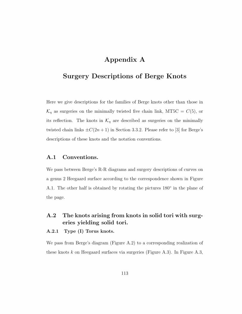
Appendix A
Surgery Descriptions of Berge Knots
Here we give descriptions for the families of Berge knots other than those in
Kη as surgeries on the minimally twisted five chain link, MT5C = C(5), or
its reflection. The knots in Kη are described as surgeries on the minimally
twisted chain links ±C(2n+ 1) in Section 3.3.2. Please refer to [3] for Berge’s
descriptions of these knots and the notation conventions.
A.1 Conventions.
We pass between Berge’s R-R diagrams and surgery descriptions of curves on
a genus 2 Heegaard surface according to the correspondence shown in Figure
A.1. The other half is obtained by rotating the pictures 180 in the plane of
the page.
A.2 The knots arising from knots in solid tori with surg-
eries yielding solid tori.
A.2.1 Type (I) Torus knots.
We pass from Berge’s diagram (Figure A.2) to a corresponding realization of
these knots k on Heegaard surfaces via surgeries (Figure A.3). In Figure A.3,
113
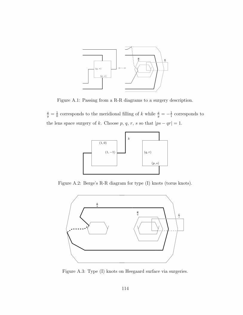
(p, s)
(q, r)
r
s
p
q
Figure A.1: Passing from a R-R diagrams to a surgery description.
xy
= 10
corresponds to the meridional filling of k while xy
= −11
corresponds to
the lens space surgery of k. Choose p, q, r, s so that |ps− qr| = 1.
(1, 0)
(p, s)
(q, r)(1,−1)
k
Figure A.2: Berge’s R-R diagram for type (I) knots (torus knots).
xy
p
q rs
Figure A.3: Type (I) knots on Heegaard surface via surgeries.
114

After dropping the Heegaard surface from the picture,we add compo-
nents with meridional framings, perform isotopies, and do Kirby Calculus as
shown in Figure A.4 to get a description of k as surgery on the MT5C.
isotopyand
two componentsadding
xy
p
q rs
xy
rs
p
q
10
10
Figure A.4: Type (I) knots. Isotopies and Kirby Calculus moves ending in theMT5C.
115
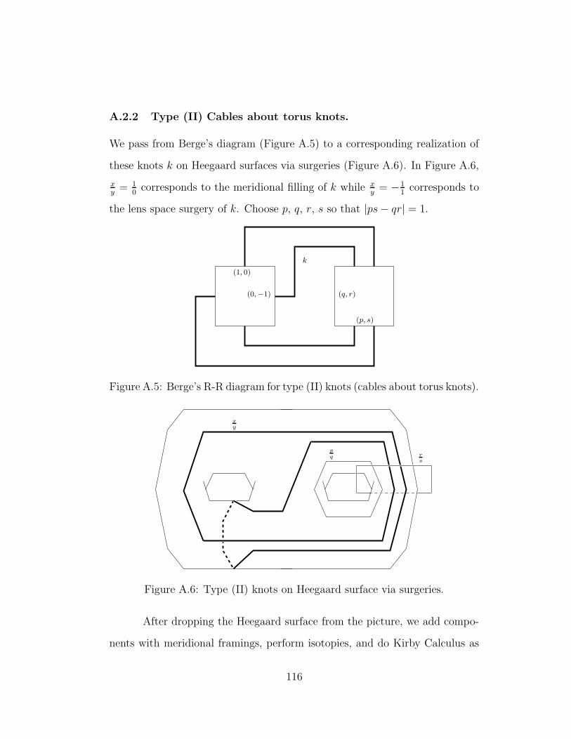
A.2.2 Type (II) Cables about torus knots.
We pass from Berge’s diagram (Figure A.5) to a corresponding realization of
these knots k on Heegaard surfaces via surgeries (Figure A.6). In Figure A.6,
xy
= 10
corresponds to the meridional filling of k while xy
= −11
corresponds to
the lens space surgery of k. Choose p, q, r, s so that |ps− qr| = 1.
(1, 0)
(p, s)
(q, r)(0,−1)
k
Figure A.5: Berge’s R-R diagram for type (II) knots (cables about torus knots).
xy
pq r
s
Figure A.6: Type (II) knots on Heegaard surface via surgeries.
After dropping the Heegaard surface from the picture, we add compo-
nents with meridional framings, perform isotopies, and do Kirby Calculus as
116
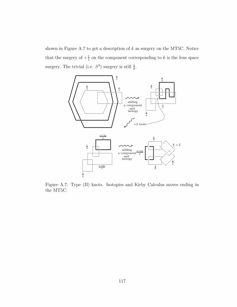
shown in Figure A.7 to get a description of k as surgery on the MT5C. Notice
that the surgery of + 11
on the component corresponding to k is the lens space
surgery. The trivial (i.e. S3) surgery is still 10.
isotopyand
a componentadding
isotopyand
a componentadding
p
q
xy
rs
+2 twist
p
q
rs
10
xy
x+2y
y
12
r+2ss
p
q
p
q10
x+2y
y
12
rs
+ 2
Figure A.7: Type (II) knots. Isotopies and Kirby Calculus moves ending inthe MT5C.
117

A.2.3 Type (III).
We pass from Berge’s diagram (Figure A.8) to a corresponding realization of
these knots k on Heegaard surfaces via surgeries (Figure A.9). In Figure A.9,
xy
= 10
corresponds to the meridional filling of k while xy
= −11
corresponds to
the lens space surgery of k. Choose p ∈ N and ε = ±1.
k
(1, 0)
(p, ε)
(2p+ ε, 2ε)(0,−1)
T
Figure A.8: Berge’s R-R diagram for type (III) knots.
1n x
y
2εε
− 1n
p
2p+ε
Figure A.9: Type (III) knots on Heegaard surface via surgeries.
The surgeries on the two parallel components in Figure A.10 can be
amalgamated into a surgery on a single component. We then drop the Hee-
118
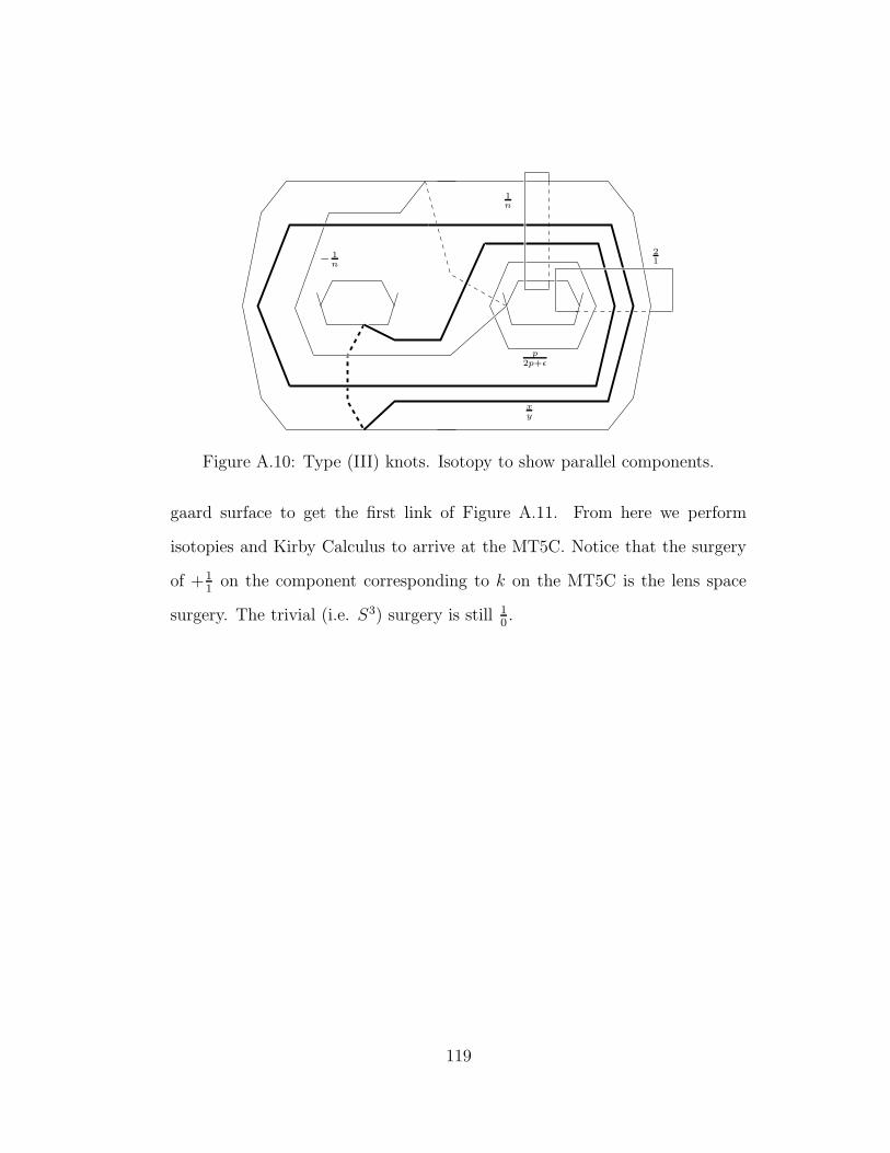
1n
21
p
2p+ε
xy
− 1n
Figure A.10: Type (III) knots. Isotopy to show parallel components.
gaard surface to get the first link of Figure A.11. From here we perform
isotopies and Kirby Calculus to arrive at the MT5C. Notice that the surgery
of +11
on the component corresponding to k on the MT5C is the lens space
surgery. The trivial (i.e. S3) surgery is still 10.
119
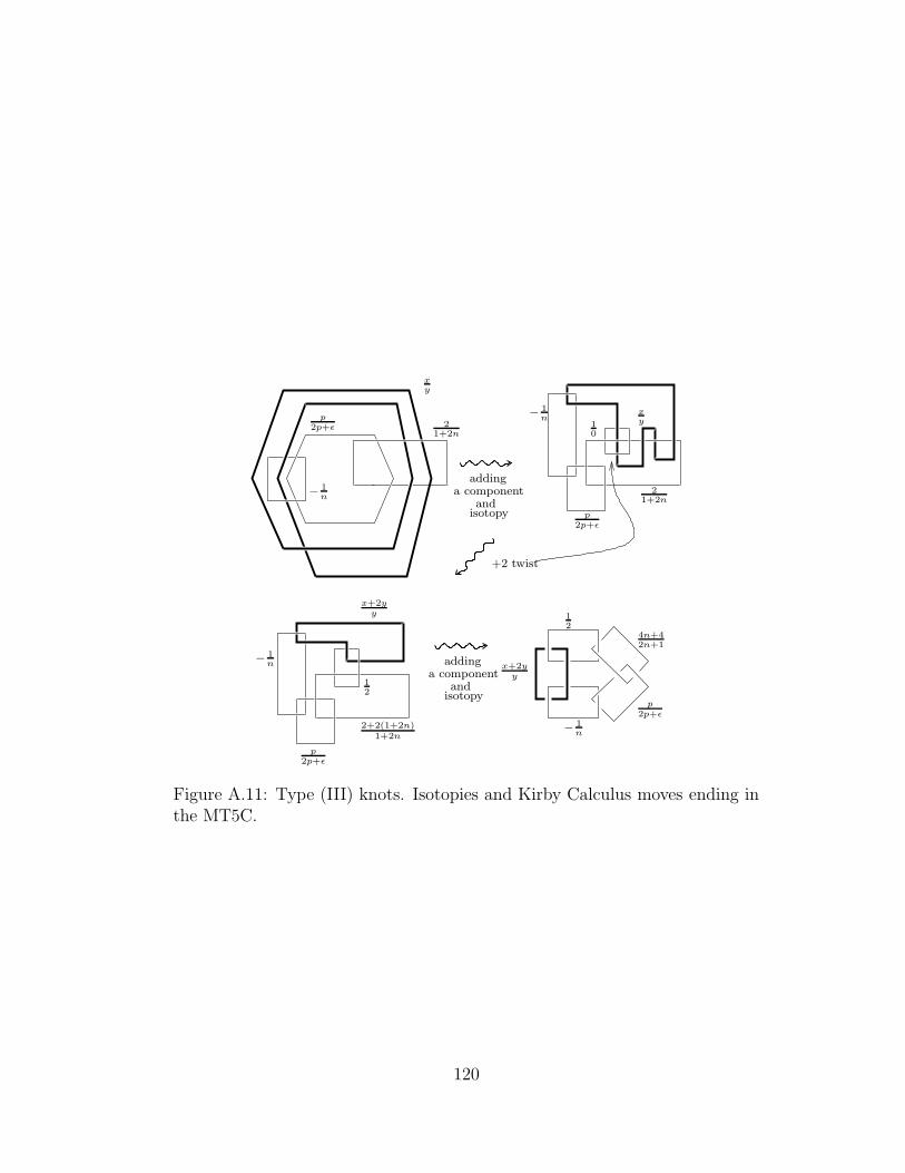
isotopyand
a componentadding
isotopyand
a componentadding
p2p+ε
− 1n
21+2n
xy
xy
21+2n
p
2p+ε
+2 twist
12
p
2p+ε
− 1n
2+2(1+2n)1+2n
p2p+ε
10
− 1n
− 1n
12
x+2y
y
4n+42n+1
x+2y
y
Figure A.11: Type (III) knots. Isotopies and Kirby Calculus moves ending inthe MT5C.
120
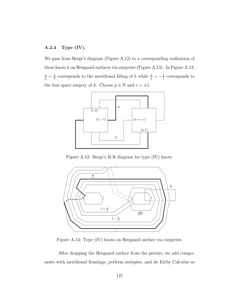
A.2.4 Type (IV).
We pass from Berge’s diagram (Figure A.12) to a corresponding realization of
these knots k on Heegaard surfaces via surgeries (Figure A.13). In Figure A.13,
xy
= 10
corresponds to the meridional filling of k while xy
= −11
corresponds to
the lens space surgery of k. Choose p ∈ N and ε = ±1.
k(1, 0)
(p, ε)
(p+ ε, ε)(1,−1)
T
Figure A.12: Berge’s R-R diagram for type (IV) knots.
xy
p
p+ε
11
1 + 1n
1 − 1n
Figure A.13: Type (IV) knots on Heegaard surface via surgeries.
After dropping the Heegaard surface from the picture, we add compo-
nents with meridional framings, perform isotopies, and do Kirby Calculus as
121

shown in Figure A.14 and continued in Figure A.15 to get a description of
k as surgery on the MT5C. Notice that the surgery of 01
on the component
corresponding to k is the lens space surgery. The trivial (i.e. S3) surgery is
still 10.
isotopyand
a componentadding
1 − 1n
xy
11
− 1n
xy− 1
−εp+ε
2 − 1n
xy
−εp
2 − 1n
2 + 1n
xy
10
−εp
+1 surgery
+1 twist
p
p+ε
1 + 1n
1n
2 + 1n
Figure A.14: Type (IV) knots. Isotopies and Kirby Calculus moves.
122
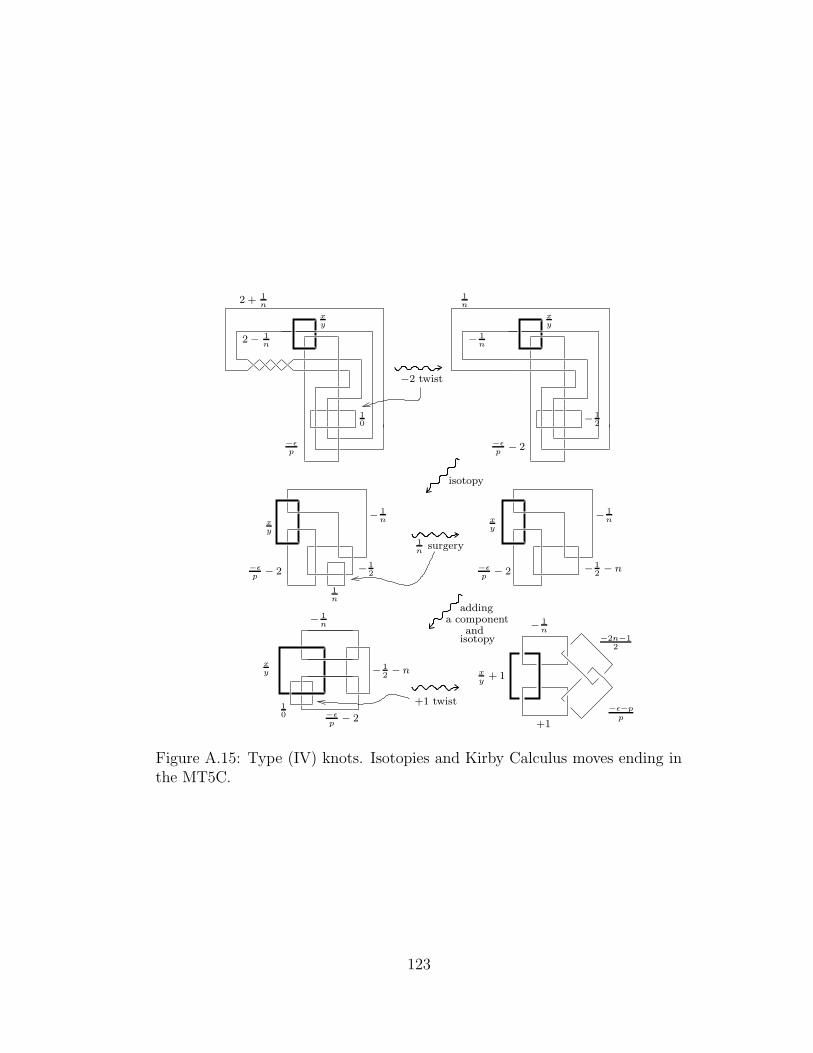
isotopyand
a componentadding
2 − 1n
xy
−2 twist
10
− 1n
xy
− 12
isotopy
− 1n
1n
− 12
1n
surgery
− 12− n
− 1n
− 1n
−2n−12
+1
−ε−p
p−εp
− 2
+1 twist
2 + 1n
−εp
1n
−εp
− 2
xy
xy
−εp
− 2 −εp
− 2
− 1n
xy − 1
2− n
10
xy
+ 1
Figure A.15: Type (IV) knots. Isotopies and Kirby Calculus moves ending inthe MT5C.
123
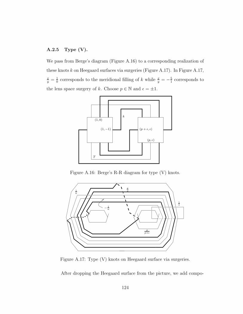
A.2.5 Type (V).
We pass from Berge’s diagram (Figure A.16) to a corresponding realization of
these knots k on Heegaard surfaces via surgeries (Figure A.17). In Figure A.17,
xy
= 10
corresponds to the meridional filling of k while xy
= −51
corresponds to
the lens space surgery of k. Choose p ∈ N and ε = ±1.
k(1, 0)
(p, ε)
(p+ ε, ε)(1,−1)
T
Figure A.16: Berge’s R-R diagram for type (V) knots.
1n
− 1n
xy
11
p
p+ε
Figure A.17: Type (V) knots on Heegaard surface via surgeries.
After dropping the Heegaard surface from the picture, we add compo-
124

nents with meridional framings, perform isotopies, and do Kirby Calculus as
shown in Figure A.18 and continued in Figure A.19 to get a description of
k as surgery on the MT5C. Notice that the surgery of 01
on the component
corresponding to k is the lens space surgery. The trivial (i.e. S3) surgery is
still 10.
125

− 1n
xy
11
pp+ε
xy− 2
−εp+ε
+1 surgery
isotopy
xy− 2
−εp+ε
−1 twist
− 1n− 1
1n− 1
xy
−εp
1n
− 1n
+ 1n
− 1n− 1
1n− 1
Figure A.18: Type (V) knots. Isotopies and Kirby Calculus moves.
126
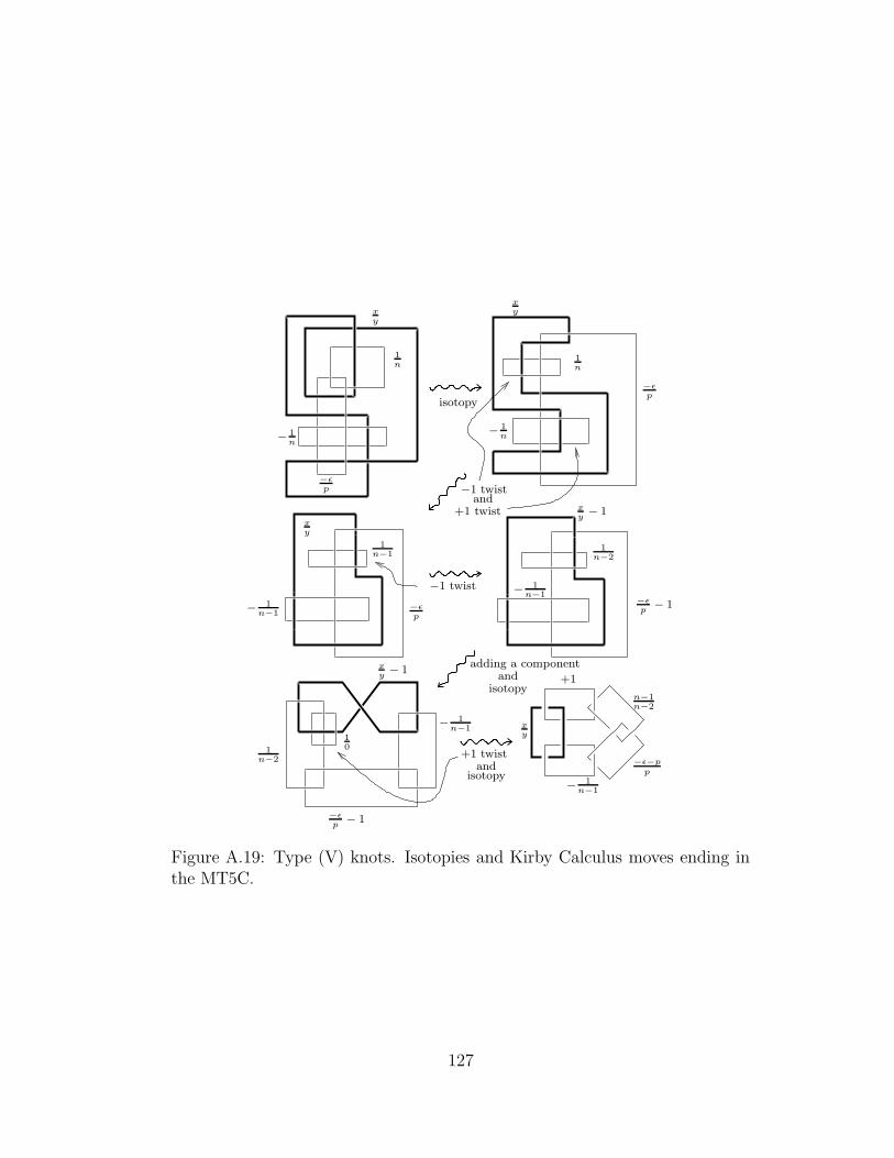
xy
1n
− 1n
−εp
isotopy
−1 twistand
+1 twist
− 1n
1n
xy
−εp
xy− 1
1n−2
−εp
− 1
− 1n−1
−εp
−1 twist
1n−1
xy
adding a componentand
isotopy
−εp
− 1
isotopyand
+1 twist
− 1n−1
+1
n−1n−2
−ε−p
p
− 1n−1
− 1n−1
xy− 1
xy
1n−2
10
Figure A.19: Type (V) knots. Isotopies and Kirby Calculus moves ending inthe MT5C.
127

A.2.6 Type (VI).
We pass from Berge’s diagram (Figure A.20) to a corresponding realization of
these knots k on Heegaard surfaces via surgeries (Figure A.21). In Figure A.21,
xy
= 10
corresponds to the meridional filling of k while xy
= −51
corresponds to
the lens space surgery of k.
k
(1, 0)
(0,−1)
(1, 0)
(3,−1)
(2,−1)
T
Figure A.20: Berge’s R-R diagram for type (VI) knots.
10
12
xy
1n
− 1n
Figure A.21: Type (VI) knots on Heegaard surface via surgeries.
After dropping the Heegaard surface from the picture, we combine some
128

of the twisting of k via the surgery of another component as shown in Figure
A.22. We continue, after an isotopy, with Kirby Calculus in Figure A.23 to
get a description of k as surgery on the MT5C. Notice that the surgery of 01
on
the component corresponding to k is the lens space surgery. The trivial (i.e.
S3) surgery is still 10.
129
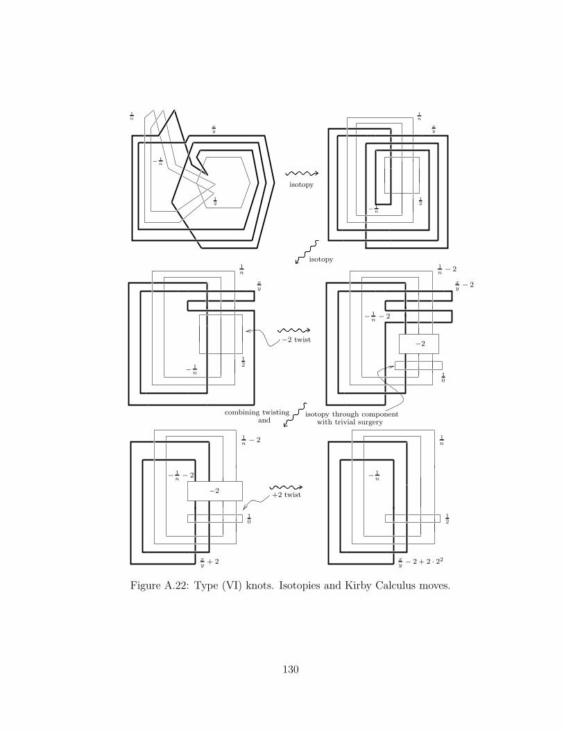
isotopy
isotopy
−2 twist
isotopy through componentwith trivial surgeryand
+2 twist
combining twisting
12
xy
1n
− 1n
−2
xy− 2
1n− 2
10
− 1n− 2
−2
10
xy
+ 2
1n− 2
− 1n− 2
12
xy− 2 + 2 · 22
− 1n
1n
12
1n
x
y
− 1n
1n
− 1n
12
x
y
Figure A.22: Type (VI) knots. Isotopies and Kirby Calculus moves.
130

xy
+ 6
+1 twist
−1 twist
− 1n
xy
+ 6
− 1n−1
adding a componentand
isotopy
1n+1
− 1n+1
xy
+ 6
10
−1
12
−1 twist
1n
12
1n+1
12
12
− nn+1
xy
+ 5
− 1n+1
Figure A.23: Type (VI) knots. Isotopies and Kirby Calculus moves ending inthe MT5C.
131
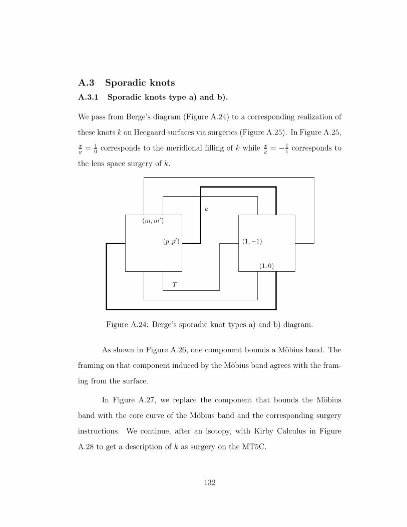
A.3 Sporadic knots
A.3.1 Sporadic knots type a) and b).
We pass from Berge’s diagram (Figure A.24) to a corresponding realization of
these knots k on Heegaard surfaces via surgeries (Figure A.25). In Figure A.25,
xy
= 10
corresponds to the meridional filling of k while xy
= −11
corresponds to
the lens space surgery of k.
k
T
(p, p′)
(m, m′)
(1, 0)
(1,−1)
Figure A.24: Berge’s sporadic knot types a) and b) diagram.
As shown in Figure A.26, one component bounds a Mobius band. The
framing on that component induced by the Mobius band agrees with the fram-
ing from the surface.
In Figure A.27, we replace the component that bounds the Mobius
band with the core curve of the Mobius band and the corresponding surgery
instructions. We continue, after an isotopy, with Kirby Calculus in Figure
A.28 to get a description of k as surgery on the MT5C.
132
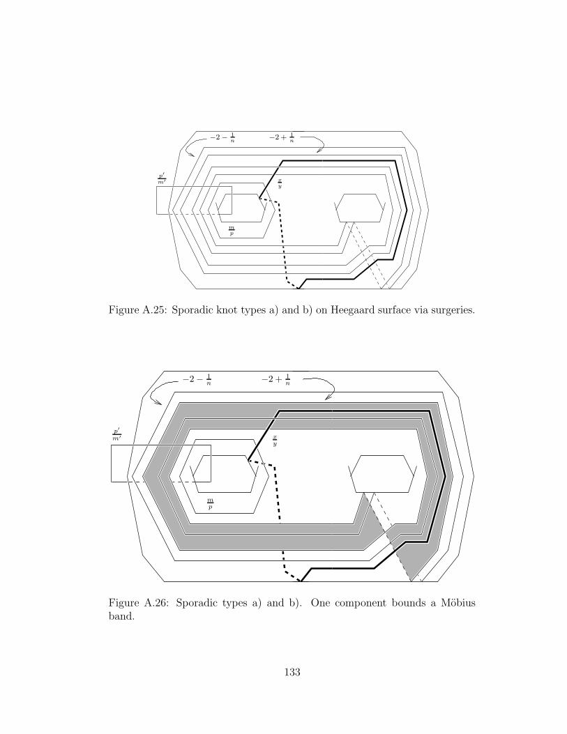
p′
m′
−2 − 1n
−2 + 1n
mp
xy
Figure A.25: Sporadic knot types a) and b) on Heegaard surface via surgeries.
p′
m′
−2 − 1n
−2 + 1n
mp
xy
Figure A.26: Sporadic types a) and b). One component bounds a Mobiusband.
133

p′
m′
mp
−2 − 1n
1−2n4n
xy
Figure A.27: Sporadic types a) and b). Core curve of Mobius band replacesthe boundary of Mobius band.
134
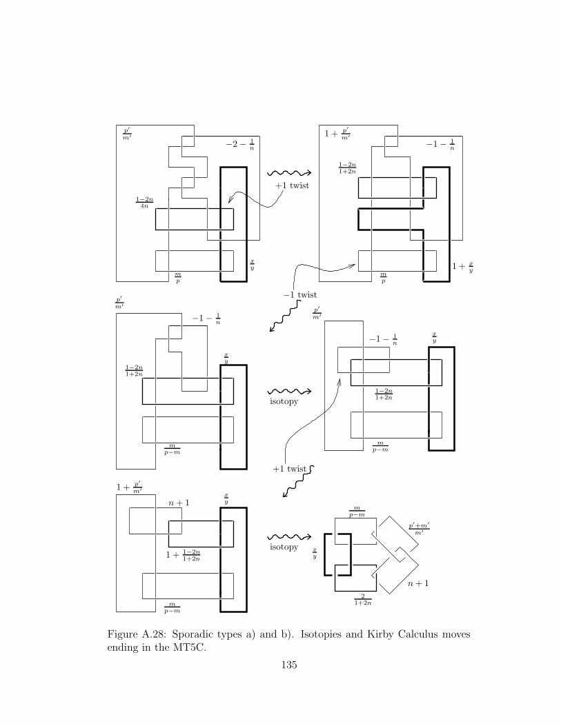
mp−m
21+2n
n + 1
p′+m′
m′
xy
1−2n4n
p′
m′
−2 − 1n
xy
mp
1 + p′
m′
−1 − 1n
mp
1 + xy
1−2n1+2n
mp−m
1−2n1+2n
p′
m′
xy−1− 1
n
p′
m′
1−2n1+2n
mp−m
xy
−1 − 1n
mp−m
1 + 1−2n1+2n
xyn + 1
1 + p′
m′
+1 twist
−1 twist
isotopy
+1 twist
isotopy
Figure A.28: Sporadic types a) and b). Isotopies and Kirby Calculus movesending in the MT5C.
135
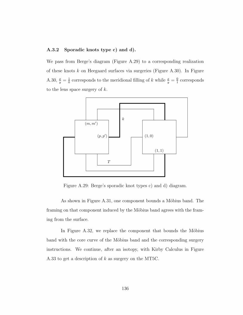
A.3.2 Sporadic knots type c) and d).
We pass from Berge’s diagram (Figure A.29) to a corresponding realization
of these knots k on Heegaard surfaces via surgeries (Figure A.30). In Figure
A.30, xy
= 10
corresponds to the meridional filling of k while xy
= 01
corresponds
to the lens space surgery of k.
k
(p, p′)
(m, m′)
(1, 1)
(1, 0)
T
Figure A.29: Berge’s sporadic knot types c) and d) diagram.
As shown in Figure A.31, one component bounds a Mobius band. The
framing on that component induced by the Mobius band agrees with the fram-
ing from the surface.
In Figure A.32, we replace the component that bounds the Mobius
band with the core curve of the Mobius band and the corresponding surgery
instructions. We continue, after an isotopy, with Kirby Calculus in Figure
A.33 to get a description of k as surgery on the MT5C.
136
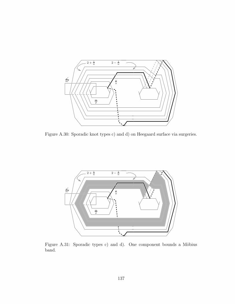
p′
m′
2 + 1n
2 − 1n
mp
xy
Figure A.30: Sporadic knot types c) and d) on Heegaard surface via surgeries.
p′
m′
2 + 1n
2 − 1n
mp
xy
Figure A.31: Sporadic types c) and d). One component bounds a Mobiusband.
137

p′
m′
2n−14n2 + 1
n
mp
xy
Figure A.32: Sporadic types c) and d). Core curve of Mobius band replacesthe boundary of Mobius band.
138

mp
1n
n − 12
p′
m′− 2
xy
2n−14n
p′
m′
2 + 1n
xy
mp
p′
m′− 2
1n
xy
mp
2n−14n−2(2n−1)
−2 twist
isotopy
Figure A.33: Sporadic types c) and d). Isotopies and Kirby Calculus movesending in the MT5C.
139
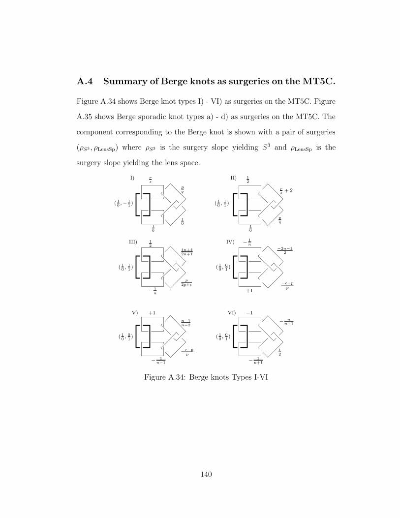
A.4 Summary of Berge knots as surgeries on the MT5C.
Figure A.34 shows Berge knot types I) - VI) as surgeries on the MT5C. Figure
A.35 shows Berge sporadic knot types a) - d) as surgeries on the MT5C. The
component corresponding to the Berge knot is shown with a pair of surgeries
(ρS3 , ρLensSp) where ρS3 is the surgery slope yielding S3 and ρLensSp is the
surgery slope yielding the lens space.
( 10,− 1
1)
I) II)
( 10, 11)
III)
( 10, 1
1)
IV)
( 10, 0
1)
V)
( 10, 0
1)
VI)
( 10, 0
1)
rs
pq
10
10
p
q10
12
rs
+ 2
12
p2p+ε
− 1n
4n+42n+1
− 1n
−2n−12
+1
−ε−p
p
+1
n−1n−2
−ε−p
p
− 1n−1
−1
12
− 1n+1
− nn+1
Figure A.34: Berge knots Types I-VI
140
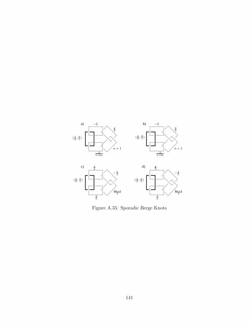
b)
c) d)
a)
( 10, 0
1)
−3
21+2n
n+ 1
32
( 10, 11)
34
1n
2n−12
− 12
( 10, 11)
23
1n
2n−12
− 13
( 10, 01)
−2
21+2n
n+ 1
43
Figure A.35: Sporadic Berge Knots
141
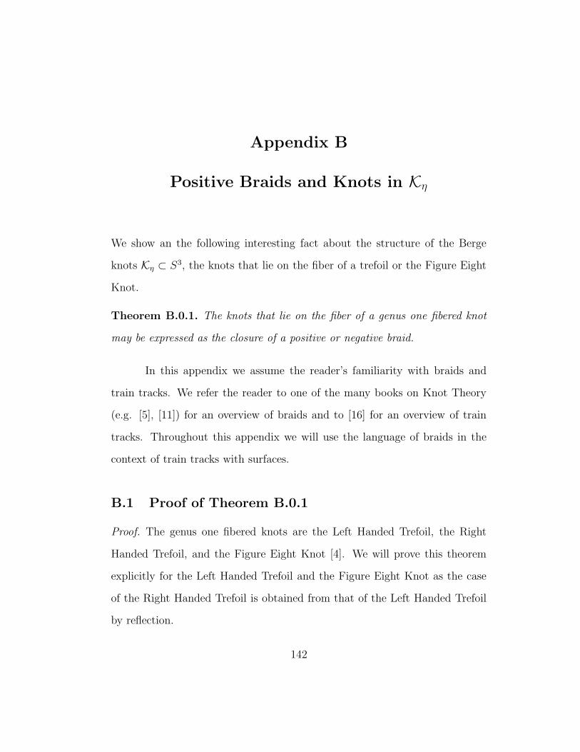
Appendix B
Positive Braids and Knots in Kη
We show an the following interesting fact about the structure of the Berge
knots Kη ⊂ S3, the knots that lie on the fiber of a trefoil or the Figure Eight
Knot.
Theorem B.0.1. The knots that lie on the fiber of a genus one fibered knot
may be expressed as the closure of a positive or negative braid.
In this appendix we assume the reader’s familiarity with braids and
train tracks. We refer the reader to one of the many books on Knot Theory
(e.g. [5], [11]) for an overview of braids and to [16] for an overview of train
tracks. Throughout this appendix we will use the language of braids in the
context of train tracks with surfaces.
B.1 Proof of Theorem B.0.1
Proof. The genus one fibered knots are the Left Handed Trefoil, the Right
Handed Trefoil, and the Figure Eight Knot [4]. We will prove this theorem
explicitly for the Left Handed Trefoil and the Figure Eight Knot as the case
of the Right Handed Trefoil is obtained from that of the Left Handed Trefoil
by reflection.
142
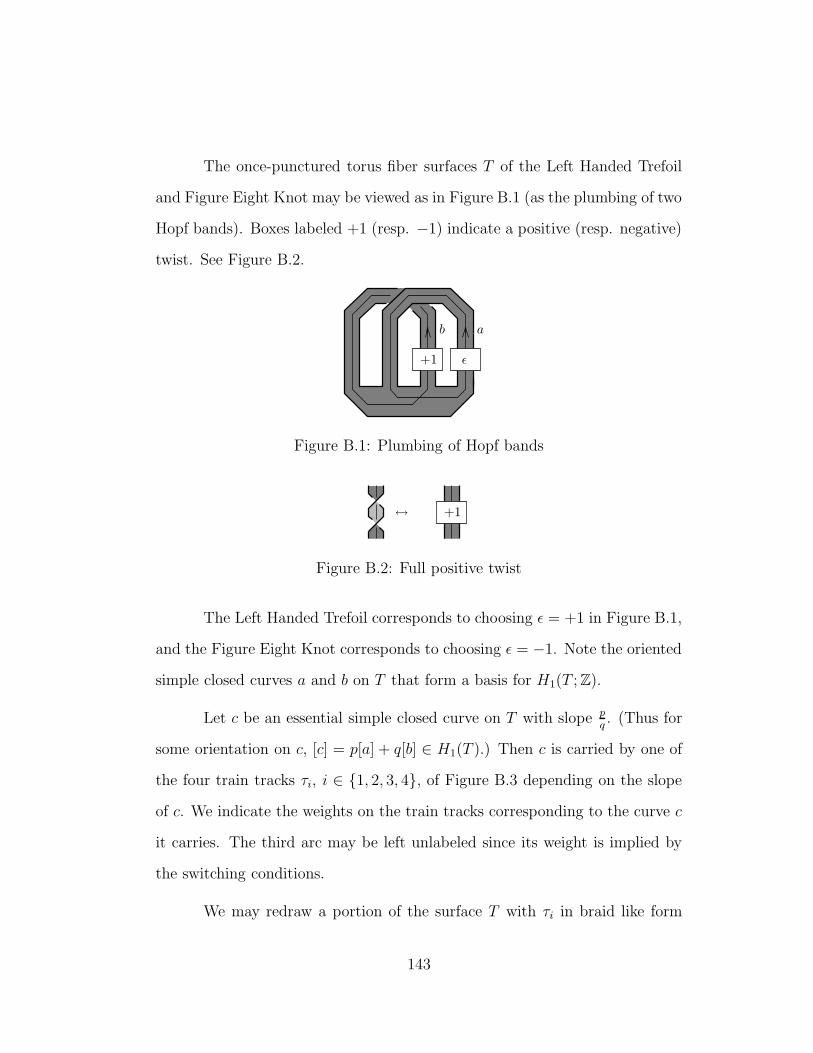
The once-punctured torus fiber surfaces T of the Left Handed Trefoil
and Figure Eight Knot may be viewed as in Figure B.1 (as the plumbing of two
Hopf bands). Boxes labeled +1 (resp. −1) indicate a positive (resp. negative)
twist. See Figure B.2.
+1
b a
ε
Figure B.1: Plumbing of Hopf bands
+1↔
Figure B.2: Full positive twist
The Left Handed Trefoil corresponds to choosing ε = +1 in Figure B.1,
and the Figure Eight Knot corresponds to choosing ε = −1. Note the oriented
simple closed curves a and b on T that form a basis for H1(T ; Z).
Let c be an essential simple closed curve on T with slope p
q. (Thus for
some orientation on c, [c] = p[a] + q[b] ∈ H1(T ).) Then c is carried by one of
the four train tracks τi, i ∈ 1, 2, 3, 4, of Figure B.3 depending on the slope
of c. We indicate the weights on the train tracks corresponding to the curve c
it carries. The third arc may be left unlabeled since its weight is implied by
the switching conditions.
We may redraw a portion of the surface T with τi in braid like form
143
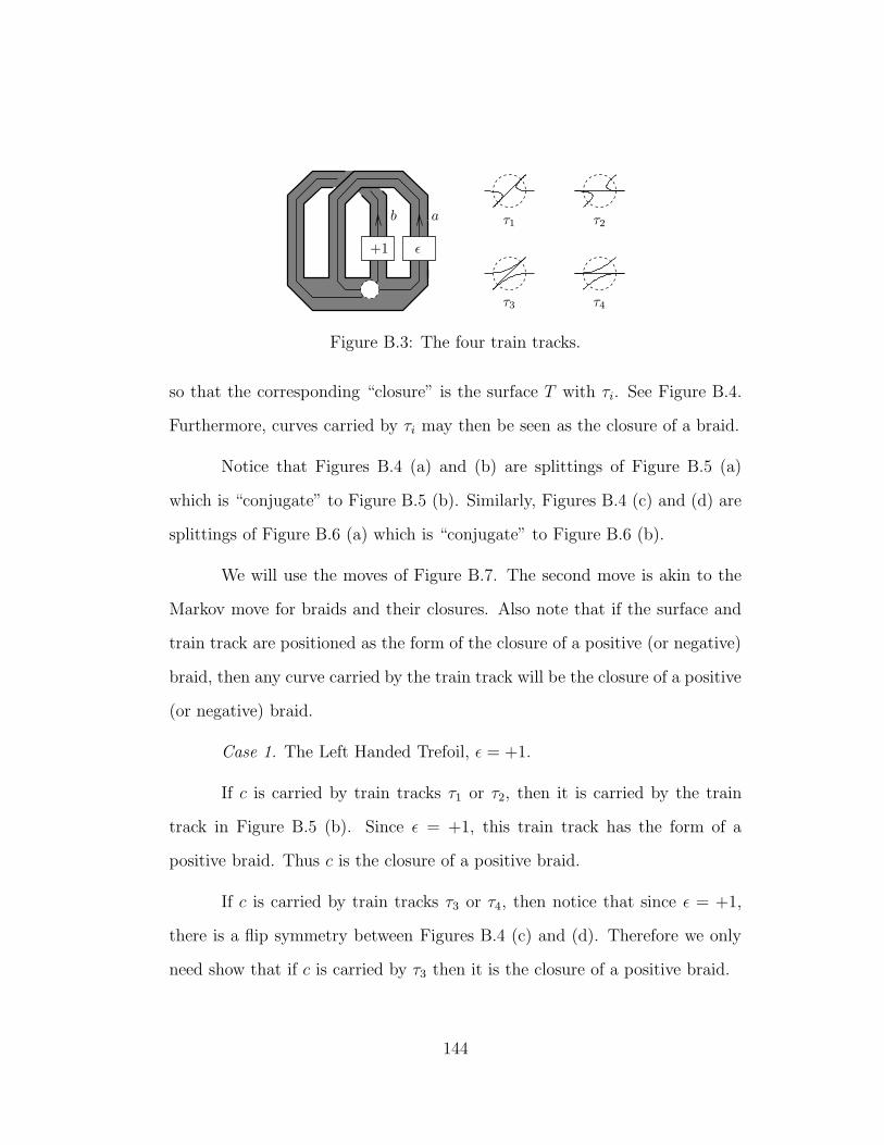
τ1 τ2
τ4τ3
+1
b a
ε
Figure B.3: The four train tracks.
so that the corresponding “closure” is the surface T with τi. See Figure B.4.
Furthermore, curves carried by τi may then be seen as the closure of a braid.
Notice that Figures B.4 (a) and (b) are splittings of Figure B.5 (a)
which is “conjugate” to Figure B.5 (b). Similarly, Figures B.4 (c) and (d) are
splittings of Figure B.6 (a) which is “conjugate” to Figure B.6 (b).
We will use the moves of Figure B.7. The second move is akin to the
Markov move for braids and their closures. Also note that if the surface and
train track are positioned as the form of the closure of a positive (or negative)
braid, then any curve carried by the train track will be the closure of a positive
(or negative) braid.
Case 1. The Left Handed Trefoil, ε = +1.
If c is carried by train tracks τ1 or τ2, then it is carried by the train
track in Figure B.5 (b). Since ε = +1, this train track has the form of a
positive braid. Thus c is the closure of a positive braid.
If c is carried by train tracks τ3 or τ4, then notice that since ε = +1,
there is a flip symmetry between Figures B.4 (c) and (d). Therefore we only
need show that if c is carried by τ3 then it is the closure of a positive braid.
144
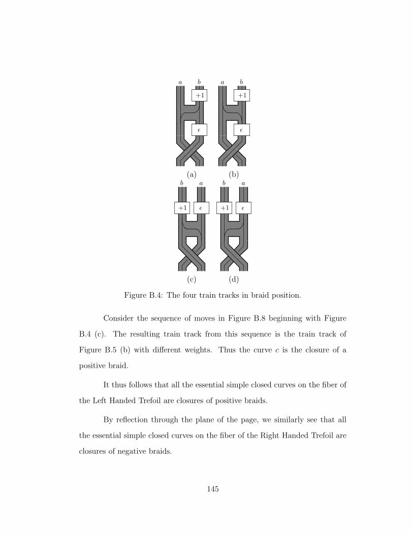
a b
ε
+1
ba
ε
+1
(a) (b)ab
ε+1
ab
ε+1
(c) (d)
Figure B.4: The four train tracks in braid position.
Consider the sequence of moves in Figure B.8 beginning with Figure
B.4 (c). The resulting train track from this sequence is the train track of
Figure B.5 (b) with different weights. Thus the curve c is the closure of a
positive braid.
It thus follows that all the essential simple closed curves on the fiber of
the Left Handed Trefoil are closures of positive braids.
By reflection through the plane of the page, we similarly see that all
the essential simple closed curves on the fiber of the Right Handed Trefoil are
closures of negative braids.
145
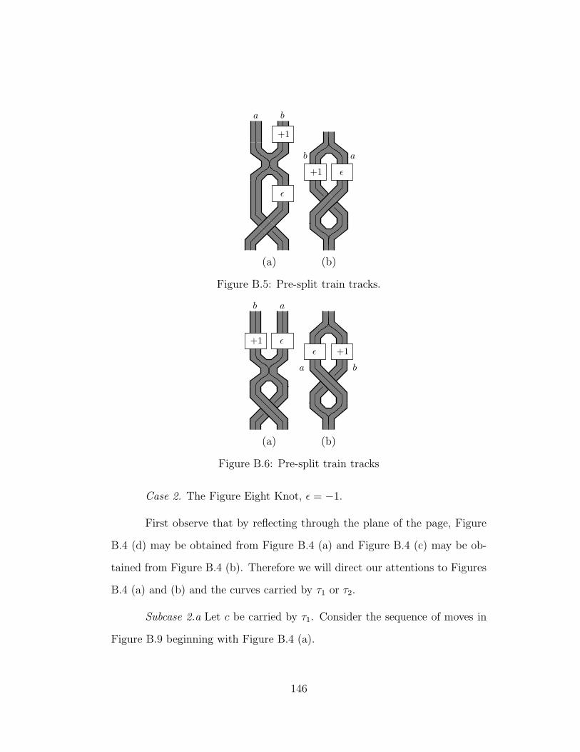
+1
ba
ε
+1 ε
b a
(a) (b)
Figure B.5: Pre-split train tracks.
+1
ab
εε +1
a b
(a) (b)
Figure B.6: Pre-split train tracks
Case 2. The Figure Eight Knot, ε = −1.
First observe that by reflecting through the plane of the page, Figure
B.4 (d) may be obtained from Figure B.4 (a) and Figure B.4 (c) may be ob-
tained from Figure B.4 (b). Therefore we will direct our attentions to Figures
B.4 (a) and (b) and the curves carried by τ1 or τ2.
Subcase 2.a Let c be carried by τ1. Consider the sequence of moves in
Figure B.9 beginning with Figure B.4 (a).
146

+1
+1 +1
↔
+1 ↔
Figure B.7: Moves for braiding train tracks on surfaces.
This move sequence concludes with the the train track being in the
form of the closure of a positive braid. Thus c is the closure of a positive
braid. (If c was carried by τ4, then due to the reflection, it is the closure of a
negative braid.)
Subcase 2.b Let c be carried by τ2. Consider the sequence of moves in
Figure B.10 beginning with Figure B.4 (b). Notice the effect on the weights.
Flipping the result over we get Figure B.6 (b) but with smaller total
weight. After a reflection of this through the plane of the page we have Figure
B.5 (b) but with smaller total weight. Thus c equivalent (up to reflection) to
a curve carried by τ1 or τ2 but with smaller total weight.
Since the above sequence of moves reduces the total weight on the train
track, repeating this process will eventually end up in Subcase 2.a or with a
147

curve carried by τ2 with weight 1 on the two labeled arcs. In the latter, the
curve is the unknot.
Therefore all the essential simple closed curves on the fiber of the Figure
Eight Knot are closures of positive or negative braids.
To summarize the conclusion of this theorem, any knot that may be
written as an essential simple closed curve on the fiber of the Left Handed
Trefoil, the Right Handed Trefoil, or the Figure Eight Knot is carried by
one of the train tracks in Figure B.11. From these one can determine the
corresponding positive or negative braid.
B.2 Consequences
Here we mention a few consequences of Theorem B.0.1. We also note that
these knots belong to the larger family of “quasipositive” knots in which Lee
Rudolph among others have had much interest.
Mind Remark 2.4.1 when correlating the following with Berge’s com-
putations of lens spaces.
B.2.1 Hopf plumbings.
By writing these knots as the closures of positive (or negative) braids, it follows
that the these knots are fibered. Furthermore these knots and their fiber can
be obtained by plumbing a collection of positive (or a collection of negative)
Hopf bands together. See [18] for one description of how this may be done.
148
B.2.2 Genera.
The fiber for these knots can be obtained from applying Seifert’s algorithm
to the diagram of the associated closure of a positive (or negative) braid rep-
resenting the knot. This makes determining the genus of the knot (i.e. the
genus of the fiber) direct.
Note that a full twist on a collection of n adjacent strands of a braid
produces n(n − 1) crossings. Furthermore, the passing of n adjacent strands
over m strands produces nm crossings.
Consider a knot k carried by the closure of the braid of Figure B.4 (a)
with ε = +1. Thus k is a knot on the Left Handed Trefoil. Since this knot is
already represented as a positive braid, an application of Seifert’s algorithm
constructs the fiber surface from a(a − 1) + b(b − 1) + ab crossings and a + b
disks. Therefore the Euler characteristic of the corresponding knot k is
χ(k) = (a + b) − (a(a− 1) + b(b− 1) + ab)
= −a2 − ab− b2 + 2(a+ b),
and its genus is
g(k) =1
2(1 + a2 + ab + b2) − (a+ b).
A similar computation can be done for the knots carried by the closure of one
of the train tracks in Figure B.11.
B.2.3 Framings.
The fiber for these knots gives the knot’s standard framing, i.e. its standard
longitude. By carrying the fiber of the Left Handed Trefoil and Figure Eight
149
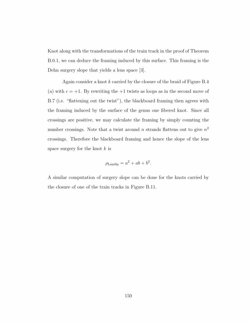
Knot along with the transformations of the train track in the proof of Theorem
B.0.1, we can deduce the framing induced by this surface. This framing is the
Dehn surgery slope that yields a lens space [3].
Again consider a knot k carried by the closure of the braid of Figure B.4
(a) with ε = +1. By rewriting the +1 twists as loops as in the second move of
B.7 (i.e. “flattening out the twist”), the blackboard framing then agrees with
the framing induced by the surface of the genus one fibered knot. Since all
crossings are positive, we may calculate the framing by simply counting the
number crossings. Note that a twist around n strands flattens out to give n2
crossings. Therefore the blackboard framing and hence the slope of the lens
space surgery for the knot k is
ρLensSp = a2 + ab + b2.
A similar computation of surgery slope can be done for the knots carried by
the closure of one of the train tracks in Figure B.11.
150
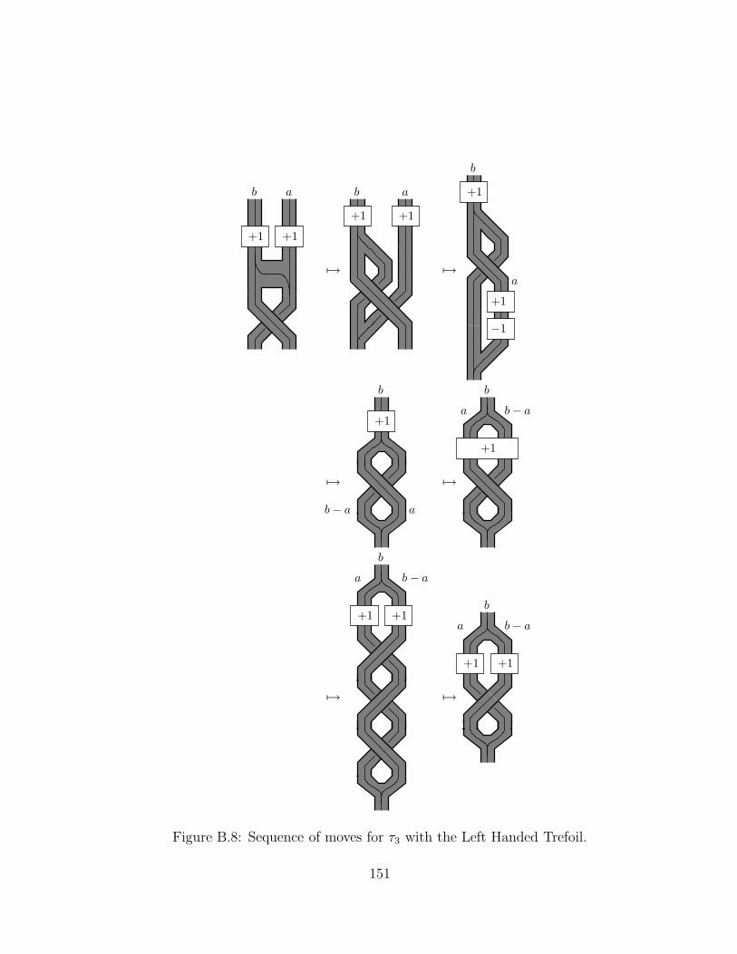
b − a
b − a
b − a
b − a
+1 +1
b a
+1
ab
+1
+1
b
a
b
+1
a
+1 +1
b
a
+1 +1
b
a
+1
+1
−1
a
b
7→ 7→
7→7→
7→7→
Figure B.8: Sequence of moves for τ3 with the Left Handed Trefoil.
151
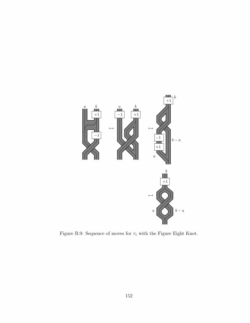
b − a
+1
+1
−1
b
a
b − a
+1−1
ba
+1
ba
−1
a
+1
b
7→ 7→
7→
Figure B.9: Sequence of moves for τ1 with the Figure Eight Knot.
152

a − b
a − b
−1 +1
ba
+1−1
a b
+1
+1
−1 −1
b
a
b
−1
a
+1
+1
−1+1
a
b
7→ 7→
7→7→
Figure B.10: Sequence of moves for τ2 with the Figure Eight Knot.
153
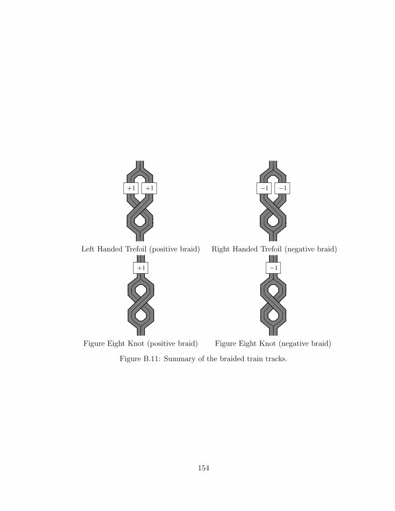
+1 +1 −1 −1
Left Handed Trefoil (positive braid) Right Handed Trefoil (negative braid)
+1 −1
Figure Eight Knot (positive braid) Figure Eight Knot (negative braid)
Figure B.11: Summary of the braided train tracks.
154
Bibliography
[1] C. Adams. Volumes of n-cusped hyperbolic 3-manifolds. J. London
Math. Soc. (2), 38(2):555–565, 1988.
[2] R. Benedetti and C. Petronio. Lectures on hyperbolic geometry. Springer-
Verlag, Berlin, 1992.
[3] John Berge. Some knots with surgeries yielding lens spaces. Alg. &
Geom. Top., X(20XX) 1-XXX, 20XX.
[4] G. Burde and H. Zieschang. Neuwirthsche knoten und flachenabbildungen.
Abh. Math. Sem. Univ. Hamburg, 1967.
[5] G. Burde and H. Zieschang. Knots. Number 5 in de Gruyter Studies in
Mathematics. Walter de Gruyter & Co., 2 edition, 2003.
[6] M. Culler, W. Jaco, and H. Rubinstein. Incompressible surfaces in once-
punctured torus bundles. Proc. London Math. Soc. (3), 45(3):385–419,
1982.
[7] W. Floyd and A. Hatcher. Incompressible surfaces in punctured-torus
bundles. Topology Appl., 13(3):263–282, 1982.
[8] C. McA. Gordon and J. Luecke. Knots are determined by their comple-
ments. Bull. Amer. Math. Soc. (N.S.), 1989.
155

[9] W. Haken. Some results on surfaces in 3-manifolds. In Studies in Modern
Topology, pages 39–98. Math. Assoc. Amer., 1968.
[10] A. Hatcher and W. Thurston. Incompressible surfaces in 2-bridge knot
complements. Invent. Math., 79(2):225–246, 1985.
[11] A. Kawauchi. A survey of knot theory. Birkhuser Verlag, 1996.
[12] R. Kirby and P. Melvin. Dedekind sums, µ-invariants and the signature
cocycle. Math. Ann., 2(299):231–267, 1994.
[13] P. Kronheimer, M. Tomasz, P. Ozsvath, and Z. Szabo. Monopoles and
lens space surgeries. ArXive:math.GT/0310164, 2003.
[14] W. B. R. Lickorish. A representation of orientable combinatorial 3-
manifolds. Ann. of Math., 1962.
[15] W. Neumann and A. Reid. Topology ’90, chapter Arithmetic of hyper-
bolic manifolds, pages 273–310. Ohio State Univ. Math. Res. Inst.
Publ., de Gruyter, Berlin, 1990.
[16] R. Penner and J. Harer. Combinatorics of train tracks. Number 125 in
Annals of Mathematics Studies. Princeton University Press, 1992.
[17] D. Rolfsen. Knots and Links. Publish or Perish, Inc., 1976, 1990.
[18] L. Rudolph. Hopf plumbing, arborescent seifert surfaces, baskets, es-
paliers, and homogeneous braids. Topology Appl., 116(3):255–277, 2001.
[19] M. Takahashi. Two-bridge knots have property p. Mem. Amer. Math.
Soc., 1981.
156

[20] W. Thurston. The Geometry and Topology of 3-manifolds. Princeton
University, 1978-80.
[21] A. Wallace. Modifications and cobounding manifolds. Canad. J. Math.,
1960.
[22] Y. Yamada. Berge’s knots in the fiber surfaces of genus one, lens spaces
and framed links. Preprint, 2003.
157
Vita
Kenneth Lee Baker was born in Austin, Texas on December 21, 1975. He grew
up in Austin and graduated from McCallum High School in June of 1994. The
next four years were spent at Rice University in Houston, Texas where he
received a B.A. in Mathematics in May of 1998. He subsequently returned
to Austin in the summer of 1998 to enter the University of Texas at Austin
Graduate School.
Permanent address: 1820 Cr 329Walburg, Texas 78626
This dissertation was typeset with LATEX‡ by the author.
‡LATEX is a document preparation system developed by Leslie Lamport as a specialversion of Donald Knuth’s TEX Program.
158