Copyright by Haomin Xu 2012

Copyright

by

Haomin Xu

2012

The Thesis Committee for Haomin Xu

Certifies that this is the approved version of the following thesis:

Potential for Non-thermal Cost-effective Chemical Augmented

Waterflood for Producing Viscous Oils

APPROVED BY

SUPERVISING COMMITTEE:

Mojdeh Delshad

Kamy Sepehrnoori

Supervisor:



by

Haomin Xu, B.S.; M.S.Engr.; D.E.

Thesis

Presented to the Faculty of the Graduate School of

The University of Texas at Austin

in Partial Fulfillment

of the Requirements

for the Degree of

Master of Science in Engineering

The University of Texas at Austin

December 2012

Dedication

To my parents

v

Acknowledgements

I am sincerely grateful to Dr. Mojdeh Delshad for the opportunity to work with

her and under her supervision over the past two years. She has provided opportunities and

helped me to immensely develop knowledge and research experience. She is essentially

an expert in the field of chemical EOR. Working directly with her has not only offered

me a thorough understanding of the respective field, but also gave me brand-new

perspectives as coming to problem solving. The core part of the research training is to be

aware of where to find the right resource. I also want to show my gratitude to Dr. Kamy

Sepehrnoori to be the reader of my thesis and to provide me with his advice and

guidance. He was always helpful and supportive through my years at graduate school.

I would like to thank laboratory researchers at UT, including Dr Do-Hoon Kim

and Robert Dean, for providing me with the coreflood design and results, based on which

I ran lab and field scale simulations. I would also like to thank the Chemical EOR

research project sponsors for not only providing financial support, but also for offers real-

time challenges to address. During my study here at UT, a few my colleagues and

officemates have also offered their help and suggestions, including but not limited to,

Zhitao Li, Vikram Chandrasekhar, Ali Goudarzi, Hariharan Ramachandran, Mohammad

Lotfollahi, Venkat Pudugramam, Peter Wang. In addition, I would like to show my

appreciation to some of the staff members at the Center for Petroleum and Geosystems

Engineering, including Joanna Castillo, Esther Barrientes, Frankie Hart, Michelle Mason,

Allison Brooks and Joanna Hall.

I would also like to acknowledge Michael Shammai and the rest of the RDS team

at Baker Hughes for giving me the opportunity to intern with them. The 10-week

vi

experience was greatly beneficial to me as I gained exposure to formation evaluation and

pressure testing, and further appreciated the way reservoir property data are collected.

I also appreciate the companionship I received from a few of my close friends

during my stay at Austin. Last but not least, my sincere and genuine gratitude goes to my

parents and family for always believing in me and supporting me unconditionally.

vii

Abstract



Haomin Xu, M.S.Engr.

The University of Texas at Austin, 2012

Supervisor: Mojdeh Delshad

Chemical enhanced oil recovery has regained its attention because of high oil

price and the depletion of conventional oil reservoirs. This process is more complex than

the primary and secondary recovery flooding and requires detailed engineering design for

a successful field-scale application.

An effective alkaline/co-solvent/polymer (ACP) formulation was developed and

corefloods were performed for a cost efficient alternative to alkaline/surfactant/polymer

floods by the research team at the department of Petroleum and Geosystems Engineering

at The University of Texas at Austin. The alkali agent reacts with the acidic components

of heavy oil (i.e. 170 cp in-situ viscosities) to form in-situ natural soap to significantly

reduce the interfacial tension, which allows producing residual oil not contacted by

waterflood or polymer flood alone. Polymer provides mobility control to drive chemical

slug and oil bank. The cosolvent added to the chemical slug helps to improve the

compatibility between in-situ soap and polymer and to reduce microemulsion viscosity.

An impressive recovery of 70% of the waterflood residual oil saturation was achieved

viii

where the remaining oil saturation after the ACP flood was reduced to only 13.5%. The

results were promising with very low chemical usage for injection. The UTCHEM

chemical flooding reservoir simulator was used to model the coreflood experiments to

obtain parameters for pilot scale simulations. Geological model was based on

unconsolidated reservoir sand with multiple seven spot well patterns.

However, facility capacity and field logistics, reservoir heterogeneity as well as

mixing and dispersion effects might prevent coreflood design at laboratory from large

scale implementation. Field-scale sensitivity studies were conducted to optimize the

design under uncertainties. The influences of chemical mass, polymer pre-flush, well

constraints, and well spacing on ultimate oil recovery were closely investigated. This

research emphasized the importance of good mobility control on project economics. The

in-situ soap generated from alkali-naphthenic acid reaction not only mobilizes residual oil

to increase oil recovery, but also enhances water relative permeability and increases

injectivity. It was also demonstrated that a closer well spacing significantly increases the

oil recovery because of greater volumetric sweep efficiency.

This thesis presents the simulation and modeling results of an ACP process for a

viscous oil in high permeability sandstone reservoir at both coreflood and pilot scales.

ix

Table of Contents

List of Tables ........................................................................................................ xi

List of Figures ..................................................................................................... xiii

CHAPTER 1: INTRODUCTION .........................................................................1

CHAPTER 2: BACKGROUND AND LITERATURE REVIEW ....................4

2.1 BACKGROUND OF CHEMICAL ENHANCED OIL RECOVERY

PROCESSES ........................................................................................4

2.1.1 Polymer Flooding ........................................................................4

2.1.2 Surfactant-Polymer (SP) Flooding ............................................5

2.1.3 Alkaline-Surfactant-Polymer (ASP) Flooding .........................5

2.2 PAST FIELD PROJECTS OF CHEMICAL FLOODING ..................6



2.2.3 Alkaline-Surfactant-Polymer (ASP) Flooding .........................8

2.3 PAST FIELD-SCALE SIMULATIONS OF CHEMICAL FLOODING

................................................................................................................9



2.3.3 Alkaline-Surfactant-Polymer (ASP) Flooding .......................10

2.4 UTCHEM SIMULATOR .....................................................................11

CHAPTER 3: LABORATORY DESIGN OF AN ALKALINE/CO-

SOLVENT/POLYMER FLOOD ...............................................................12

3.1 CORE PROPERTIES AND COREFLOOD DESIGN .......................12

3.2 PCN-1 COREFLOOD HISTORY MATCH WITH UTCHEM ........27

3.3 PCN-1 COREFLOOD HISTORY MATCH WITH CMG STARS .37

3.4 PCN-4 COREFLOOD HISTORY MATCH WITH UTCHEM .......41

3.5 SUMMARY AND CONCLUSIONS ....................................................50

x

CHAPTER 4: PILOT-SCALE DESIGN OF AN ALKALINE/CO-

SOLVENT/POLYMER FLOOD ...............................................................52

4.1 SIMULATION MODEL .......................................................................52

4.2 BASE CASE SIMULATION ................................................................61

4.3 SENSITIVITY SIMULATION STUDIES ..........................................67

4.3.1 Sensitivity to ACP Slug Size .....................................................71

4.3.2 Sensitivity to Polymer Drive Size.............................................73

4.3.3 Sensitivity to Injection Rates....................................................74

4.3.4 Sensitivity to Polymer Adsorption ...........................................75

4.3.5 Sensitivity to Alkaline Retention .............................................76

4.3.6 Sensitivity to Chemical Concentrations during ACP ............77

4.3.7 Sensitivity to Polymer Concentrations for Mobility Buffer ..78

4.3.8 Sensitivity to Polymer Preflush (PPF).....................................80

4.3.9 Sensitivity to Pressure Constraint Injectors ...........................82

4.3.10 Polymer Flooding (PF) ...........................................................89

4.3.11 Sensitivity to Well Spacing .....................................................91

4.4 DETERMINATION OF THE OPTIMUM ACP DESIGN ..............................102

4.5 SUMMARY AND CONCLUSIONS ........................................................102

CHAPTER 5: SUMMARY AND CONCLUSIONS .......................................104

Appendix A: Salinity Gradient .........................................................................106

Appendix B: Input File of CMG STARS Model for PCN-1 Coreflood ........107

Appendix C: Input File of UTCHEM Base Case Pilot-Scale Simulation .....131

Glossary ..............................................................................................................180

References ...........................................................................................................181

xi

List of Tables

Table 3-1. Bentheimer Core Properties. ............................................................15

Table 3-2. Compositions of Synthetic Brine (PCNSSB). ..................................15

Table 3-3. ACP Slug and Polymer Drive (PD) Coreflood Design....................16

Table 3-4. Co-solvent and Soap Phase Behavior Input Parameters. ..............27

Table 3-5. Polymer Input Parameters. ...............................................................28

Table 3-6. Input Parameters for Co-solvent/Microemulsion Properties. .......29

Table 3-7. Bentheimer Core Properties. ............................................................42

Table 3-8. Composition of Synthetic Softened Brine (PCNSSB). ....................42

Table 3-9. ACP Slug and Polymer Drive (PD) Coreflood Design....................43

Table 3-10. Co-solvent and Soap Phase Behavior Input Parameters. ............47

Table 3-11. Polymer Input Parameters. .............................................................47

Table 3-12. Key Input Parameters for Co-surfactant/Microemulsion Properties.

...........................................................................................................47

Table 4-1. List of Simulation Model Properties. ...............................................59

Table 4-2. List of Cosolvent and Polymer Parameters. ....................................60

Table 4-3. Base Case ACP Flood Design. ...........................................................62

Table 4-4. Economic Analysis Input Parameters. .............................................71

Table 4-5. List of Simulations for ACP Slug Size Sensitivity. ..........................72

Table 4-6. List of Simulations for PD Slug Size Sensitivity. ............................73

Table 4-7. List of Simulations for Injection Rates Sensitivity. ........................74

Table 4-8. List of Simulations for Polymer Adsorption Sensitivity.................76

Table 4-9. List of Simulations for Alkaline Retention Sensitivity. ..................77

Table 4-10. List of Simulations for Chemical Conc. Sensitivity during ACP.78

xii

Table 4-11. List of Simulations with Various Polymer Conc. during Mobility

Buffer. ..............................................................................................79

Table 4-12. List of Simulations for Polymer Preflush Slug Size Sensitivity. ..81

Table 4-13. List of Simulations for Pressure Constraint Sensitivity. ..............83

Table 4-14. List of Polymer Flood Simulations. ................................................90

Table 4-15. List of Simulations for Well Spacing Sensitivity. ..........................93

Table 4-16.Sensitivity Simulation Economic Analysis. .....................................99

xiii

List of Figures

Figure 3-1. ACP Coreflood and Pressure Transducer Setup. .........................14

Figure 3-2. Activity Diagram with 1.5% n-Butyl-5EO. ....................................17

Figure 3-3. Microemulsion Viscosity with 1.5% Butyl-5EO in PCNSSB at 16,000

ppm TDS in 30% Oil. .....................................................................18

Figure 3-4. Total Relative Mobility and Viscosity Requirement. ....................19

Figure 3-5. ACP Slug Viscosity at Two Shear Rates. .......................................20

Figure 3-6. Viscosity of Polymer Drive with Salinity of 1,000 ppm TDS at Two

Shear Rates. .....................................................................................21

Figure 3-7. ACP Slug Viscosity with 0.6% Na2CO3 (6,934 ppm TDS) at 38 oC.22

Figure 3-8. Oil Recovery, Oil Saturation, and Oil Cut for PCN-1 Coreflood.23

Figure 3-9. Effluent pH and Oil Cut for PCN-1 Coreflood..............................24

Figure 3-10. Effluent Samples of PCN-1 Coreflood. .........................................25

Figure 3-11. Bentheimer Sandstone Core after PCN-1 Chemical Flood. .......26

Figure 3-12. Relative Permeability Curves Based on Coreflood History Match.

...........................................................................................................30

Figure 3-13. Cumulative Oil Recovery for PCN-1 Coreflood. .........................31

Figure 3-14. Oil Cut for PCN-1 Coreflood. .......................................................31

Figure 3-15. Oil Saturation Curve for PCN-1 Coreflood. ................................32

Figure 3-16. Pressure Drop of Entire Core for PCN-1 Coreflood. ..................32

Figure 3-17. Effect of ME Viscosity Model on Pressure Drop. ........................33

Figure 3-18. Cumulative Oil Recovery with and without Co-solvent Adsorption.

...........................................................................................................34

Figure 3-19. Oil Cut with and without Co-solvent Adsorption. ......................35

xiv

Figure 3-20. Oil Saturation with and without Co-solvent Adsorption. ...........36

Figure 3-21. Pressure Drop with and without Co-solvent Adsorption. ..........37



Figure 3-24. Oil Saturation for PCN-1 Coreflood.............................................40


Figure 3-26. Activity Diagram with 3.0% Iso-Butyl-10EO at 38 oC. ..............44

Figure 3-27. Polymer Drive Viscosity in PCNSSB brine (10,934 ppm TDS), 38

oC. .....................................................................................................45

Figure 3-28. Calculated Relative Permeability Curve Based on PCN-4 Coreflood.

...........................................................................................................46



Figure 3-31. Oil saturation for PCN-4 Coreflood. ............................................49


Figure 4-1. Permeability in md of Layer 1. .......................................................53

Figure 4-2. Permeability in md in Layer 3. .......................................................54

Figure 4-3. Permeability in md in Layer 5. .......................................................55

Figure 4-4. Oil Saturation in Layer 1. ................................................................56



Figure 4-7. Base Case – Cumulative Oil Production. .......................................63

Figure 4-8. Base Case – Total Production Rate and Oil Cut. ..........................64

Figure 4-9. Base Case – Oil Saturation after Polymer Drive (Layer 1). .........65

Figure 4-10. Base Case – Oil Saturation after Polymer Drive (Layer 3). .......66

xv

Figure 4-11. Base Case – Oil Saturation after Polymer Drive (Layer 5). .......67

Figure 4-12. Injection Rate of Well 1 with 5,000 psi BHP................................84






Figure 4-18. Cumulative Oil Production of ACP + PD vs. Polymer Flood. ...91

Figure 4-19. Cumulative Oil Recovery for Various Well Spacing. .................94

Figure 4-20. Oil Saturation of Layer 1 at the End of ACP Flood of Case 3-12-1

(Base Case). ......................................................................................95


(Base Case). ......................................................................................96


(25% Well Spacing). .......................................................................97


(25% Well Spacing). .......................................................................98

1

CHAPTER 1: INTRODUCTION

In most conventional oil reservoirs, the oil recovery factor during the primary

recovery phase by natural mechanisms is typically 5-15%. Approximately 30% of the

original oil in place can be recovered from the secondary recovery such as waterflood,

depending on the properties of the oil and the characteristics of the reservoir rock. The

remaining original oil in place (between 55 and 65%) cannot be economically produced

due to the pore capillary forces, low sweep efficiency because of reservoir heterogeneity

and insufficient mobility of flow at reservoir conditions. With the current high crude oil

price and lower recovery costs compared to 1960s, enhanced oil recovery (EOR)

processes become viable techniques to produce the large fraction of the oil trapped or

bypassed in the reservoir.

Lake (1989) defined EOR as injecting fluids that are not typically present in the

reservoir to improve sweep efficiency. It can be achieved by miscible gas injection,

chemical injection, microbial injection, or thermal recovery. Chemical EOR works by

adding a combination of chemical agents, e.g. alkali, surfactant, co-solvent, and polymer

to the injected water to improve fluid mobility and to reduce interfacial tension (IFT)

between injected fluid and crude oil. There have been a number of successful field-scale

tests since the 1960s. With the current high oil price, it is receiving more and more

attention on technology development and application. In this thesis, chemical EOR

processes will be simulated for a high-permeability low-temperature sandstone reservoir

to optimize the design to maximize its cumulative oil recovery.

During chemical EOR, polymers are used to improve the mobility of injected

water to increase the volumetric sweep efficiency. Surfactants are used to lower the IFT

2

or capillary pressure that traps oil droplets from being produced from a reservoir,

ultimately improving local displacement sweep efficiency. Alkali is used to generate in-

situ soap that would further lower IFT to enhance oil production from reservoirs with

crude oil that has organic acids. A number of important factors (e.g. the residual oil

saturation, the acid number of crude oil, reservoir rock properties, reservoir fluid

properties, reservoir heterogeneity, or field operational conditions) dictate the right slug

design for a successful chemical EOR process to produce residual oil economically

beyond waterflood.

Once chemical EOR is chosen as the proper candidate for EOR, it is important to

conduct test tubes experiments in laboratory to fully understand the phase behavior and to

screen for the most promising chemical formulation for the target reservoir conditions.

Screening is based on salinity, surfactant, co-solvent (if any), and oil concentrations.

Outcrop and reservoir coreflood are then run to demonstrate the oil recovery efficiency at

reservoir temperature. Numerical simulation is essential for a successful design because

of the process complexity of chemical EOR and uncertainties in reservoir

characterization. Reservoir simulators such as UTCHEM could help to history match the

laboratory measurements to obtain the key process parameters that govern the physical

and transport properties of the chemical agents used, and eventually transfer the model

into field-scale. The objective of this thesis is to optimize the pilot-scale design based on

coreflood model by investigating the impact of various design parameters of alkaline/co-

solvent/polymer (ACP) flood on the cumulative oil recovery in pilot area. Co-solvent

helps to improve the compatibility between polymer and surfactant and to reduce the

chemical loss due to adsorption onto the rock. Of course, a successful laboratory

coreflood on reservoir core might not always scale up to the field-scale due to reservoir

heterogeneity, or chemical retention, mixing and dispersion effects. The results from this

3

thesis could certainly reduce the risk of reservoir uncertainties and help to finalize an

optimum and robust design for the target reservoir.

Here is a short introduction of the following chapters within this thesis. Chapter 2

provides a brief description of the chemical EOR processes and documents a literature

review of the previous EOR field-scale projects and simulations. Chapter 3 presents the

detailed laboratory results of an ACP coreflood. In order to optimize the chemical slug

design, Chapter 4 identifies key parameters that affect cumulative oil recovery in a high-

permeability, low temperature sandstone reservoir. Chapter 5 summarizes the important

finding of this thesis.

4

CHAPTER 2: BACKGROUND AND LITERATURE REVIEW

2.1 BACKGROUND OF CHEMICAL ENHANCED OIL RECOVERY

PROCESSES

2.1.1 Polymer Flooding

The mobility in a multiphase system is defined as the ratio of the effective

permeability to the viscosity of that phase, as shown in Eq. 1.

(1)

The mobility ratio is defined as the ratio of the mobility of the displacing phase to

the mobility of the displaced phase. The mobility of the fluids for each phase can be

calculated by adding up the mobility of each fluid respectively. The total mobility ratio is

presented in Eq. 2.

∑

∑ (2)

In most hydrocarbon recovery processes, the mobility of the displacing phase is

typically larger than that of the displaced phase. This will cause the displacing phase to

bypass displaced phase and leave most of the pore volume unswept leading to lower

volumetric sweep efficiency as the result of viscous fingering and channeling. In order

to overcome this effect, water soluble polymers are injected to increase the viscosity (i.e.

to lower the mobility) of the displacing water phase to be equal to or less than the

mobility of the displaced oil phase so that mobility ratio, sweep efficiency and fractional

flow can be greatly improved (Pope, 1980). As one of the most common methods of

EOR, approximately one billion pounds of polymer were consumed for EOR operations

in 2011 (Pope, 2011). With the improvement of its product quality at a cheaper price

5

relative to crude oil, hydrolyzed polyacrylamide (HPAM) (i.e. one of the most commonly

used commercial polymers) becomes more favorable in field applications, along with its

insensitiveness to biodegradation. In addition, polymer molecules obtain tolerance to

divalent ions and high salinity and protection to hydrolysis at high temperatures by

adding monomers (Vermolen et al., 2011).

2.1.2 Surfactant-Polymer (SP) Flooding

During an SP flooding, surface-active agent (surfactant) is injected to reduce the

interfacial tension (IFT) between water (displacing phase) and oil (displaced phase), and

hence mobilize the residual oil saturation beyond that of waterflood. Polymer is added to

the chemical slug to improve the volumetric sweep efficiency and the SP slug is chased

by polymer drive to ensure that the injected chemicals are effectively displaced through

the reservoir. Chatzis and Morrow (1984) proposed that the amount of residual oil that

can be mobilized is associated with capillary number, i.e. the ratio of viscous forces to

capillary forces. Surfactant development has advanced remarkably since the start of

surfactant flooding. A wide selection of cost-effective surfactants that can be tailored to

tolerate harsh environmental (high salinity high temperature reservoirs) and reduce IFT

by up to five orders of magnitude are now available on market (Adkins et al., 2010).

Hirasaki et al. (2008) summarized the significant breakthrough in the development of

surfactant technology. Anionic surfactants are favored to SP field tests, mostly performed

in sandstone reservoirs since they are repelled by negative charges associated with

sandstone rock surface at neutral pH and that leads to lower surfactant adsorption.

2.1.3 Alkaline-Surfactant-Polymer (ASP) Flooding

The ASP flood consists of injecting an alkaline agent (most commonly sodium

carbonate), surfactant, and polymer during the chemical slug in reservoirs that contains

6

oil with sufficient fraction of naphthenic acids. The alkali generates soap in-situ by

reaction between the alkali and naphthenic acids in the crude oil. Hirasaki et al. (2011)

published surfactant adsorption data where significantly reduced in both sandstone and

carbonate formations by the injection of alkali such as sodium carbonate. The same

chemicals can also alter the wettability of carbonate formations from strongly oil-wet to

preferentially water-wet. The combined effects of ultralow IFT and wettability alteration

make it possible to displace oil from preferentially oil-wet carbonate matrix to fractures

by oil/water gravity drainage.

2.2 PAST FIELD PROJECTS OF CHEMICAL FLOODING

As discussed in the previous chapter, reservoir heterogeneity and capillary force

are the primary factors that adversely affect waterflood efficiency, and therefore,

additives are required to overcome these effects. Detling (1944) was the first researcher

to patent the use of water-soluble additives to improve the mobility ratio, while Atkinson

and Adams (1927) first patented the use of chemicals to reduce IFT. Pye (1963) initiated

the application of viscoelastic HPAM to improve oil recovery. Johnson (1975) initially

defined mechanism of injecting alkali to enhance oil recovery. Nelson et al. (1984) used a

co-surfactant with a higher salinity requirement for Type III phase behavior to address

poor alkali propagation and uncertainties in the in-situ soap phase behavior on the field-

scale. Falls et al. (1994) reported the recovery of at least 38% of the waterflood residual

oil by cosurfactant-enhanced alkaline flooding and without polymer for mobility control

at White Castle field. Numerous successful worldwide field-scale chemical flooding

(Polymer, SP and ASP) projects have been documented in the literature.

7


Koning et al. (1988) reported a total oil production of 59% STOIIP from Al

Khlata formation of Marmul field.

Takagi et al. (1992) history matched the results of polymer flood field test at the

Courtenay sand of Chateaurenard field in France. The pilot test is characterized by high

oil recovery (i.e. 1.5 bbls oil per lbm polymer), as a combined result of large volume of

polymer, favorable reservoir and fluid conditions, and excellent design and field

operation.

Wang et al. (2002) reported the incremental recovery in the range of 12 – 15%

OOIP by polymer flooding at Daqing field, primarily due to the increase in displacement

efficiency and volumetric sweep efficiency. Wang et al. (2008) mentioned that another 2

– 4% of OOIP can be produced with profile modification before polymer injection.


Gilliland and Conley (1976) reported a pilot SP field test at the Big Muddy field

in Wyoming. The reservoir was a low-pressure watered out sandstone with economically

high residual oil saturation after waterflood that favors subsequent chemical flooding.

They achieved an oil cut increase from 1% during waterflood to 19% at peak oil

production rate.

Putz et al. (1980) reported a pilot SP field test that recovered 68% of residual oil

saturation at Chateaurenard field in France. Holm and Robertson (1980) and Widmeyer et

al. (1988) reported successful pilot field tests as well.

Bragg et al. (1982) reported a pilot SP field test in a watered out sandstone

reservoir at Loudon field in Fayette County, IL. The key technical success in this pilot

test is that they produced approximately 60% of the residual oil saturation after

8

waterflood, remarkably at the presence of high salinity formation water (104,000 ppm

TDS) without the employment of the water preflush.

Bae (1985) reported a SP field test in a shallow and low permeability sandstone

reservoir at Glenn Pool field in Creek and Tulsa counties, OK. They successfully

produced about one-third of the residual oil saturation after waterflood.

A number of chemical flooding field projects in carbonate reservoirs have been

reported in the literature since the early 70’s. Complex reservoir conditions, e.g. high

heterogeneity, low porosity and permeability, make it difficult to characterize limestone

or dolomite reservoirs. In addition, carbonate reservoirs are typically oil-wet, fracture or

both. Technical success to increase oil recovery greatly favors the application of chemical

EOR on carbonate reservoirs, but the high marginal costs eliminate almost all benefits

from the increased production. Adams et al. (1987), as one of the few successful

examples, presented a pilot SP flooding field test at San Andres dolomite reservoir in

West Texas, during which the residual oil saturations to chemical flooding were 7.5%

and 18% respectively for the two well pairs. It showed that both surfactant formulations

can overcome the heterogeneity, low permeability, and formation brine with high salinity

and hardness in a carbonate environment. Generally speaking, the application of chemical

flooding in carbonate reservoirs is complicated by increased uncertainties.


Clark et al. (1993) implemented an ASP design on the West Kiehl Unit at Crook

County, WY. The design was based on laboratory coreflood that recovered 23% OOIP

beyond waterflood.

9

Qu et al. (1998) reported a successful application of ASP flooding pilot on

Gudong field, China, which is characterized by severe heterogeneity and high oil

viscosity. They increased the ultimate oil recovery by 13.4% OOIP within the pilot area.

Qiao et al. (2000) reported a success of performing an ASP pilot test at Karamay

field, i.e. highly heterogeneous conglomerate reservoirs, in China. An increase of 24%

OOIP in the incremental oil recovery was achieved, primarily due to the combination of

both ultra-low IFT and proper mobility control.

Vargo et al. (1999), Wang et al. (1999), Manrique et al. (2000) and many other

researchers have also reported successful ASP field tests. Gao and Gao (2010)

documented the test results of different ASP flooding at Karamay, Daqing and Shengli

fields. The incremental oil recovery for these field tests ranges from 13.4% − 35.3% of

OOIP.

2.3 PAST FIELD-SCALE SIMULATIONS OF CHEMICAL FLOODING


Takagi et al. (1992) reached a good agreement between the simulations using

UTCHEM and field performance of the Courtenay polymer pilot in the Chateaurenard

field located south of Paris, France. Sensitivity studies reported that the polymer pilot

performance was dominated by polymer adsorption, while the oil recovery was

insensitive to changes in the permeability distribution or graded polymer injection

scheme, meaning fingering was not important.


Saad et al. (1989) used UTCHEM to history match the surfactant/polymer pilot

project at the Big Muddy field near Casper, WY. From simulations results, the salinity

gradient during preflush for this fresh water reservoir and the incurring Sodium-calcium

10

exchange with the clays which shifted the electrolyte concentration from the designed

Type I phase behavior to optimum Type III, played a major role in the project success. As

a result, IFT reduction and residual oil mobilization were achieved. Huh et al. (1990)

matched the performance of three SP flood pilot tests of 0.71, 40, and 80 acres carried out

at the Loudon field, IL. Simulations suggested that lower injection concentrations of

polymer in the larger pilots led to poor polymer bank propagation due to retention, and

hence ineffective oil recovery. Greater heterogeneity and low permeability regions would

further decrease the oil displacement efficiency. There were additional problems in

larger pilots with biopolymer degradation despite the addition of biocides for bacteria

control.


Qu et al. (1998) conducted a history match of waterflood and ASP flooding in

Gudong oilfield located in the area of Yellow River delta, China. The successful design

and operation of ASP flooding in the field increased 13.4% OOIP, or 30% ROIP. The

simulation results using UTCHEM provided a detailed understanding of the alkali and

surfactant phase behavior as well as the mechanisms of ASP flooding. Based on history

match, sensitivity studies were performed on the impacts of design parameters, e.g.

chemical agent types, chemical concentrations, or slug sizes, on the oil recovery of ASP

flooding. The studies showed that higher chemical concentrations and smaller slug size

led to a higher oil recovery under conditions of equivalent chemical usage.

Hernandez et al. (2001) used a simulator (GCOMP) to history match ASP

coreflood in laboratory and run numerical simulations to predict the field performance of

ASP flood to reduce the risk of field implementation. Design optimization was conducted

11

in order to achieve maximum oil recovery as well as to meet the capacity of surface

facilities.

Zerpa et al. (2005) performed an optimization study to maximize the cumulative

oil recovery from a heterogeneous and multiphase petroleum reservoir that is subject to

an ASP flooding. The combination of numerical simulations and economic calculations

was used to determine key parameters (e.g. chemical agent types, chemical

concentrations and slug size) in an effort to optimize final field design.

2.4 UTCHEM SIMULATOR

The reservoir simulator used in this thesis is UTCHEM, a three-dimensional,

multiphase, multicomponent chemical flooding simulator developed in the Center for

Petroleum and Geosystems Engineering at The University of Texas at Austin (Pope et al.,

1979; Data-Gupta et al., 1986; Saad et al., 1989; Bhuyan et al., 1990; Delshad et al.,

1996; Delshad et al., 2006). The solution scheme of UTCHEM solves pressure implicitly

and saturation explicitly. In the simulator, the flow and mass-transport equations are

solved to simulate any number of user-specified chemical components, e.g. water, oil,

surfactant, co-solvent, polymer, cations, anions and tracers. It also accounts for all of the

significant phenomena such as microemulsion phase behavior, three-phase relative

permeability, capillary desaturation of oil, water and microemulsion phases, shear-

thinning and viscoelastic polymer viscosity, adsorption, cation exchange, tracer

partitioning and reaction, geochemical reactions, gel reactions, and temperature-

dependent phase behavior. It has been widely used for a large number of EOR

applications, including polymer, surfactant/polymer (SP) and alkaline/surfactant/polymer

(ASP) flooding, tracer tests and gel treatments.

12

CHAPTER 3: LABORATORY DESIGN OF AN ALKALINE/CO-

SOLVENT/POLYMER FLOOD

The performance of the ACP formulation to recover crude oil from a Bentheimer

core at the reservoir temperature of 38 °C was evaluated in the laboratory (Kim et al.,

2011). The chemical formulation was developed from aqueous and microemulsion phase

behavior tests at 38 °C using synthetic softened brine (PCNSSB) and surrogate crude oil

diluted with 7.5 wt% Decalin to achieve similar properties as the live oil. The viscosity of

the diluted oil is approximately 170 cP at the reservoir temperature. Flopaam 3630S was

used in the chemical slug to improve mobility control and to get a better volumetric

sweep of the core. The aqueous stability of this formulation in the presence of 1000 ppm

HPAM Flopaam 3630S polymer from SNF is more than 56,000 ppm TDS. Even though

the optimum salinity is 16,000 ppm TDS, the salinity of 7,000 ppm TDS was chosen for

ACP slug by considering the activity of the crude and viscous microemulsion slightly

above the optimum salinity. From the coreflood results, the oil recovery was 69.5% of

residual oil saturation after waterflood and residual oil saturation from chemical flood

(Sorc) was 13.5%. The pressure drop at steady state looked reasonable with 5.5 psi across

the whole core of 1 ft length. The result was not great, but seemed to be promising with

very low usage of chemicals such as co-solvent, alkali and polymer.

3.1 CORE PROPERTIES AND COREFLOOD DESIGN

ACP coreflood is a complex experiment and it takes constant attention from

scientists and researchers in laboratory at UT to obtain good results. They generously

provided us with the coreflood results (PCN-1 and PCN-4) presented in this section,

including design and setup, core properties, test tube phase behavior, and polymer

13

properties. All the simulation and modeling results of this ACP process for a viscous oil

at both lab and field scale in the following chapters are based on PCN-1 coreflood. Its

common procedure is summarized as following. Figure 3-1 shows the ACP coreflood

transducer setup.

1) The core was measured for mass before saturation.

2) The core was vacuumed and tested for leaks.

3) The core was then saturated with formation brine and measured for saturated mass

to determine the pore volume of the core.

4) The core was placed in a 38 C oven and allowed to equilibrate

5) Water with salinity similar to the formation brine (PCNSFB) was injected at 10

ml/min to measure the brine permeability at 38 C.

6) Field surrogate crude oil was injected at a constant pressure of 50 psi and 38 C to

saturate the core, and residual water saturation was measured.

7) The ACP and polymer drive slugs will be mixed and filtered

8) Phase behavior pipettes will be made with the ACP slug at 30% oil concentration

to test the formulation

9) The core was then water flooded with PCNFB at the flow rate of 5 ft/day at 38 C

until 99% water cut. Residual oil saturation (Sor) was determined by mass balance;

and water permeability (Kwater) was determined by end point pressure drop.

10) The core was pre-flooded with PCNSB brine (1000 ppm TDS) to reduce the brine

salinity.

11) The ACP and polymer drive slug viscosities and filtration ratio were measured.

12) The ACP slug was injected at 38 C at a flow rate of 1 ft/day.

13) The ACP slug was followed by polymer drive at 38 C at the same flow rate until

no more oil or emulsion is produced.

14) The oil recovery and pressure drop were measured. pH and viscosities of effluent

samples were measured.

15) Core will be checked for visual indication of remaining oil and its location.

14

Figure 3-1. ACP Coreflood and Pressure Transducer Setup.

The Bentheimer sandstone core fitted at both ends with end caps for fluid

injection/collection. There are five pressure taps along the core so that pressure can be

monitored across different sections of the core while the core flood is underway. The core

has been epoxy coated and cured at 38 °C to ensure the structural integrity of the core at

high temperature. The core has a length of 11.99" and a diameter of 1.97". Tables 3-1, 3-

2 and 3-3 summarize the core properties, the ACP slug and polymer drive (PD) design as

well as the synthetic brine composition for this coreflood experiment.

ASP Core Flood Setup

0-40 psi

0-40 psi

0-40 psi

0-150 psi

0-40 psi

0-300 psi

Out to fraction retriever

3

2

1

4 0-150 psi

Back

Pressure

Regulator

15

Table 3-1. Bentheimer Core Properties.

Temperature, oC 38

Length, ft 0.971129

Diameter, ft 0.164167

Pore Volume, ft3 0.004944

Porosity 0.21

Permeability, md 2507

Initial Oil Saturation before ACP 0.443

Residual Water Saturation 0.17

Water Relative Permeability 0.07

Oil Relative Permeability 0.95

Table 3-2. Compositions of Synthetic Brine (PCNSSB).

Ion Concentration (ppm)

Potassium 11.59

Sodium 300.00

Magnesium 0

Calcium 0

Chlorine 140.81

Sulfate 310.41

Bicarbonate 176.95

Total Dissolved Solid 939.77

16

Table 3-3. ACP Slug and Polymer Drive (PD) Coreflood Design.

ACP Slug Polymer Drive

0.5 PV 1.4 PV

1.5% Huntsmann n-Butyl-5EO 2250 ppm Flopaam 3630S in PCNSSB

(934 ppm TDS)

6,000 ppm Na2CO3 in PCNSSB (6,934 ppm

TDS)

Frontal velocity : 1 ft/day

2750 ppm Flopaam 3630S Viscosity: ~140 cp @ 5 s-1

, 38 oC

Frontal velocity: 1 ft/day

Viscosity: ~ 100 cp @ 5 s-1

, 38 oC

The phase behavior of the co-solvent formulation composed of 1.5% Butyl-5EO

at 38 °C was studied using a Na2CO3 scan in PCNSSB brine using 7.5% decalin-diluted

crude oil at volume fractions ranging from 10-50% oil. The optimal salinity is 16000 ppm

TDS at 30-50% Oil and 11,000 ppm TDS at 10% oil concentrations. The TDS

concentration is the sum of PCNSSB brine and added alkali and the TDS of PCNSSB

brine is 939.77 ppm. The activity map for the crude oil based on the phase behavior data

with this co-solvent formulation is presented in Figure 3-2. The activity map shows a

negative slope and a wide Type III range. The aqueous solution composed of this co-

solvent formulation with 1000 ppm Flopaam 3630s is clear at 38 °C at a TDS more than

36000 ppm at 38 °C. Microemulsion viscosity with 30% oil was measured at different

shear rates at the optimum salinity of 16,000 ppm TDS and it is around 90 cp where the

7.5% Decalin-diluted oil to mimic the live oil, has a viscosity of ~ 170 cp at the reservoir

temperature of 38 °C (Figure 3-3). This indicates that the selected formulation generates a

good microemulsion phase with reasonable viscosity and ultralow IFT.

17

Figure 3-2. Activity Diagram with 1.5% n-Butyl-5EO.

18

Figure 3-3. Microemulsion Viscosity with 1.5% Butyl-5EO in PCNSSB at 16,000

ppm TDS in 30% Oil.

Figure 3-4 shows a peak of approximately 180 cp for the inverse total relative

mobility plot suggesting that the viscosity of the slug and polymer drive needs to be at

least 180 cp at a given shear rate of 5 s-1

corresponding to 1 ft/day. The Flopaam 3630S

polymer’s viscosity was then estimated at a range of concentrations in PCNSSB in order

to determine the concentration necessary for the ACP slug and polymer drive (as shown

in Figures 3-5 − 3-7).

10-2 10

-110

010

1

102

101

102

Rate [s-1]

h

()

[c

P]

PCN-106 ME 16000 ppm 30% oil steady

19

Figure 3-4. Total Relative Mobility and Viscosity Requirement.

20

Figure 3-5. ACP Slug Viscosity at Two Shear Rates.

21

Figure 3-6. Viscosity of Polymer Drive with Salinity of 1,000 ppm TDS at Two Shear

Rates.

22

Figure 3-7. ACP Slug Viscosity with 0.6% Na2CO3 (6,934 ppm TDS) at 38 oC.

During the coreflood, 0.5 PV ACP slug was injected at a rate of 1 ft/day chased

by a polymer drive at the same velocity until no more oil is produced. Effluent samples

were collected in graduated tubes with an average sample size of 5 mL. The pH and

viscosity were measured on the effluent samples at regular intervals. The pH of the

effluent was measured for every fourth sample. The effluent viscosities were measured

for a couple of samples at steady state to check the degradation of polymer compared

with that injected. Figures 3-8 and 3-9 show the oil recovery, the oil saturation, the oil cut

and the effluent pH measurements in the laboratory. Figures 3-10 and 3-11 present the

effluent samples and the Bentheimer sandstone core after chemical flood.

23

Figure 3-8. Oil Recovery, Oil Saturation, and Oil Cut for PCN-1 Coreflood.

0%

10%

20%

30%

40%

50%

60%

70%

80%

90%

100%

0.00 0.20 0.40 0.60 0.80 1.00 1.20 1.40 1.60 1.80 2.00Pore Volumes

Cu

m O

il R

eco

vere

d (

%)

0%

5%

10%

15%

20%

25%

30%

35%

40%

45%

50%

Oil S

atu

rati

on

(%

)

Cum Oil

Oil Cut

So

Emulsion (Soap)

Breakthrough

PCN-01 ACP Flood

0.5 PV

ACP Slug

(0.6 % Na2CO3@ PCNSSB)

1.5 PV

Polymer Drive @ PCNSSB

24

Figure 3-9. Effluent pH and Oil Cut for PCN-1 Coreflood.

0%

10%

20%

30%

40%

50%

60%

70%

80%

90%

100%

0.00 0.25 0.50 0.75 1.00 1.25 1.50 1.75 2.00

Pore Volumes

Oil C

ut

(%)

2.00

3.00

4.00

5.00

6.00

7.00

8.00

9.00

10.00

11.00

12.00

pH

Oil Cut pH

Emulsion

(Soap)

Breakthrough

PCN-1 ACP Flood

25

Figure 3-10. Effluent Samples of PCN-1 Coreflood.

26

Figure 3-11. Bentheimer Sandstone Core after PCN-1 Chemical Flood.

27

3.2 PCN-1 COREFLOOD HISTORY MATCH WITH UTCHEM

UTCHEM version 2011 and CMG STARS were used to history match the PCN-1

and PCN-4 coreflood measured results, including cumulative oil recovery, oil cut, oil

saturation, and pressure drop, as shown in Sections 3.2, 3.3 and 3.4. In this chapter, the

UTCHEM simulation of PCN-1 coreflood provides input parameters that would best

represent co-surfactant and in-situ soap phase behavior, polymer and co-

solvent/microemulsion properties. Tables 3-4, 3-5 and 3-6 summarize the key UTCHEM

model input parameters for this coreflood.

Table 3-4. Co-solvent and Soap Phase Behavior Input Parameters.

Input Parameters Value

HBNC70 0.15

HBNC71 0.13

HBNC72 0.15

CSEL7, meq/ml 0.1415

CSEU7, meq/ml 0.2264

IMIX 0

CSELP, meq/ml 0.2

CSEUP, meq/ml 0.33

28

Table 3-5. Polymer Input Parameters.


AP1 50

AP2 150

AP3 1200

SSLOPE -0.4435

GAMAC 4

GAMHF, GAMHF2 10, 0

POWN 2.3

BRK 100

CRK 0

29

Table 3-6. Input Parameters for Co-solvent/Microemulsion Properties.


ALPHAV1 0.1

ALPHAV2 1.7

ALPHAV3 0.1

ALPHAV4 0

ALPHAV5 0

AD31 1.6

AD32 0.1

B3D 1000

AD41 0.48

AD42 0

B4D 100

The endpoint relative permeability of water and oil are 0.07 and 0.95 respectively.

The residual saturation is 0.17 for water and 0.443 for oil. The exponents for water and

oil phases are determined from the coreflood history match, which will be discussed in

great details in the next section. They are 6 and 1.5 respectively. Figure 3-12 shows the

relative permeability of water and oil phase present in the core assuming the exponents

based on coreflood history match. It is important to note that the plot is not from lab

measurements, but from calculations using UTCHEM input parameters.

30

Figure 3-12. Relative Permeability Curves Based on Coreflood History Match.

Figures 3-13 – 3-16 show that UTCHEM gives a good match of cumulative oil

recovery, oil cut and oil saturation. Combined effects of polymer concentration on

microemulsion viscosity and shear thinning behavior of microemulsion phase might

cause the higher simulated pressure drop in Figure 3-16 than measured experimental data.

0

0.1

0.2

0.3

0.4

0.5

0.6

0.7

0.8

0.9

1

0 0.1 0.2 0.3 0.4 0.5 0.6

Re

lati

ve P

erm

eab

ility

Sw

krw

kro

31

Figure 3-13. Cumulative Oil Recovery for PCN-1 Coreflood.

Figure 3-14. Oil Cut for PCN-1 Coreflood.

0%

10%

20%

30%

40%

50%

60%

70%

80%

0 0.5 1 1.5 2

Cu

m O

il R

eco

vere

d, %

OO

IP

Pore Volumes

Lab

UTCHEM

0%

10%

20%

30%

40%

50%

60%

70%

80%

0 0.5 1 1.5 2

Oil

Cu

t

Pore Volumes

Lab

UTCHEM

32

Figure 3-15. Oil Saturation Curve for PCN-1 Coreflood.

Figure 3-16. Pressure Drop of Entire Core for PCN-1 Coreflood.

To further investigate the mismatch of pressure drop, we implemented a

microemulsion viscosity without the effect of polymer . The results show negligible

differences in terms of oil recovery, oil cut, and oil saturation. However, Figure 3-17

0%

10%

20%

30%

40%

50%

0 0.5 1 1.5 2

Oil

Satu

rati

on

Pore Volumes

Lab

UTCHEM

0

2

4

6

8

10

12

0 0.5 1 1.5 2

Pre

ssu

re D

rop

(p

si)

Pore Volumes

Lab

UTCHEM

33

shows that this modification leads to much lower pressure drop across the core.

Microemulsion viscosity measurements are needed in order to develop a more accurate

microemulsion phase viscosity for viscous oils in the presence of viscous polymer and

surfactant or in-situ soap.

Figure 3-17. Effect of ME Viscosity Model on Pressure Drop.

It has later come to our attention that the high pressure drop across the 1 ft core

acted more like clogging or high molecular weight particles blocking the pores within the

reservoir rock. In accordance to its property, however, co-solvent has almost minimum

adsorption onto rocks. We ran simulation with zero co-solvent adsorption and compare

the results with the base case. Figures 3-18 − 3-20 present slight differences in

cumulative oil recovery, oil cut, and oil saturation between the two simulations. Yet the

0

2

4

6

8

10

12

0 0.5 1 1.5 2

Pre

ssu

re D

rop

(p

si)

Pore Volumes

Lab

Original ViscosityModel

New ViscosityModel

34

model without co-solvent adsorption has pressure drop much closer to the lab

measurement (Figure 3-21).

Figure 3-18. Cumulative Oil Recovery with and without Co-solvent Adsorption.

35

Figure 3-19. Oil Cut with and without Co-solvent Adsorption.

36

Figure 3-20. Oil Saturation with and without Co-solvent Adsorption.

37

Figure 3-21. Pressure Drop with and without Co-solvent Adsorption.

3.3 PCN-1 COREFLOOD HISTORY MATCH WITH CMG STARS

CMG-STARS is a thermal, K-value compositional, chemical reaction and

geomechanics reservoir simulator ideally suited for advanced modeling of recovery

processes involving the injection of steam, solvents, air, and chemicals. Therefore, it

was used to benchmark against UTCHEM for comparison. All the coreflood design

parameters, including core properties, test tube phase behavior and polymer properties,

were transferred directly from UTCHEM model to CMG STARS. The CMG STARS

input file for PCN-1 coreflood is given in Appendix B. Figures 3-22 through 3-24

presented the cumulative oil recovery, oil cut and oil saturation for PCN-1 coreflood,

showing good history match results from CMG STARS model. There seems numerical

38

instability with CMG STARS simulation in specific evident in the pressure drop. We

tried to improve this by adjusting the time steps and other numerical convergence input

parameters, as shown in Figure 3-25.


0%

10%

20%

30%

40%

50%

60%

70%

80%

0 0.5 1 1.5 2

Cu

m O

il R

eco

vere

d, %

OO

IP

Pore Volumes

Lab

CMG STARS

39


0%

10%

20%

30%

40%

50%

60%

70%

80%

90%

100%

0 0.5 1 1.5 2

Oil

Cu

t

Pore Volumes

CMG STARS

Lab

40

Figure 3-24. Oil Saturation for PCN-1 Coreflood.

0%

5%

10%

15%

20%

25%

30%

35%

40%

45%

50%

0 0.5 1 1.5 2

Oil

Satu

rati

on

Pore Volumes

Lab

CMG STARS

41


3.4 PCN-4 COREFLOOD HISTORY MATCH WITH UTCHEM

The performance of a similar formulation (iso-Butyl-10EO) was evaluated in

another Bentheimer coreflood. It was used for PCN-4 coreflood in order to provide

optimum salinity gradient to mobilize the oil from the reservoir core. The aqueous

stability of this formulation in the presence of 1000 ppm FP 3630S polymer is beyond

45,000 ppm Na2CO3. The optimal salinity is 30,000 ppm Na2CO3 at 50% Oil, 30,000

ppm Na2CO3 at 30% oil and 26,000 ppm Na2CO3 at 10% oil concentrations. The core

was aged at 78 oC for 6 weeks. The waterflood was performed using synthetic produced

brine, PCNSFB (38,234 ppm TDS) to prevent any clay swelling by injecting fresh water.

The salinity for ACP slug is chosen at 30,000 ppm Na2CO3 (30,934 ppm TDS) by

considering low IFT and microemulsion viscosity. And the salinity for polymer drive is

-1

0

1

2

3

4

5

6

7

0 0.5 1 1.5 2

Pre

ssu

re D

rop

(p

si)

Pore Volumes

CMG STARS

Lab

42

chosen at 10,000 ppm Na2CO3 (10,934 ppm TDS) to prevent any clay swelling in the

reservoir rock when fresh water is injected. Tables 3-7, 3-8 and 3-9 summarize the core

properties, the design of ACP slug and polymer drive (PD), as well as the synthetic brine

formulations for this PCN-4 coreflood.

Table 3-7. Bentheimer Core Properties.

Temperature, oC 38

Length, ft 0.91667

Diameter, ft 0.125

Pore Volume, ft3 0.00315

Porosity 0.28

Permeability, md 1500

Initial Oil Saturation before ACP 0.36

Residual Water Saturation 0.36

Water Relative Permeability 0.03

Oil Relative Permeability 1

Table 3-8. Composition of Synthetic Softened Brine (PCNSSB).

Ion

Concentration

(ppm)

Potassium 11.59

Sodium 300.00

Magnesium 0

Calcium 0

Chlorine 140.81

Sulfate 310.41

Bicarbonate 176.95

TDS 939.77

43

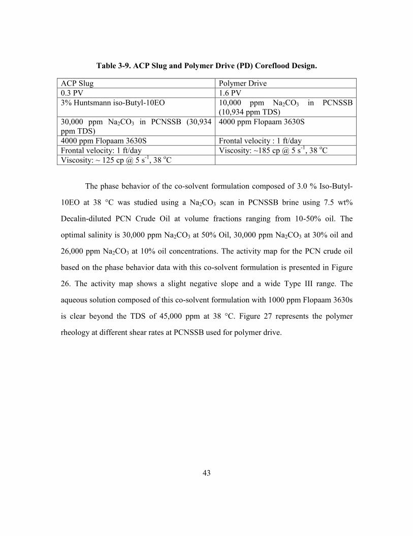
Table 3-9. ACP Slug and Polymer Drive (PD) Coreflood Design.

ACP Slug Polymer Drive

0.3 PV 1.6 PV

3% Huntsmann iso-Butyl-10EO 10,000 ppm Na2CO3 in PCNSSB

(10,934 ppm TDS)

30,000 ppm Na2CO3 in PCNSSB (30,934

ppm TDS)

4000 ppm Flopaam 3630S

4000 ppm Flopaam 3630S Frontal velocity : 1 ft/day

Frontal velocity: 1 ft/day Viscosity: ~185 cp @ 5 s-1

, 38 oC

Viscosity: ~ 125 cp @ 5 s-1

, 38 oC

The phase behavior of the co-solvent formulation composed of 3.0 % Iso-Butyl-

10EO at 38 °C was studied using a Na2CO3 scan in PCNSSB brine using 7.5 wt%

Decalin-diluted PCN Crude Oil at volume fractions ranging from 10-50% oil. The

optimal salinity is 30,000 ppm Na2CO3 at 50% Oil, 30,000 ppm Na2CO3 at 30% oil and

26,000 ppm Na2CO3 at 10% oil concentrations. The activity map for the PCN crude oil

based on the phase behavior data with this co-solvent formulation is presented in Figure

26. The activity map shows a slight negative slope and a wide Type III range. The

aqueous solution composed of this co-solvent formulation with 1000 ppm Flopaam 3630s

is clear beyond the TDS of 45,000 ppm at 38 °C. Figure 27 represents the polymer

rheology at different shear rates at PCNSSB used for polymer drive.

44

Figure 3-26. Activity Diagram with 3.0% Iso-Butyl-10EO at 38 oC.

0

10000

20000

30000

40000

50000

60000

0% 10% 20% 30% 40% 50% 60%

So

diu

m C

arb

on

ate

Co

ncen

trati

on

(p

pm

)

Oil Concentration (wt%)

Activity Map - After 43 Days at 38 ºC3% IBA-10EO

Type I

Type III

Type II

45

Figure 3-27. Polymer Drive Viscosity in PCNSSB brine (10,934 ppm TDS), 38 oC.

The endpoint relative permeability of water and oil for this Bentheimer core are

measured as 0.03 and 1 respectively. The residual saturation is 0.36 for water and 0.36

for oil. The exponents for water and oil phases are determined from the coreflood history

match as 6 and 1.1 respectively. Figure 28 shows the relative permeability of water and

oil present in the core. It is important to note that the plot is not from lab measurement,

but from calculation using UTCHEM input parameters based on history match.

10-3 10

-210

-110

010

110

2

103

101

102

103

104

Rate [s-1]

h

()

[c

P]

PCN-04R PD plus dithionite

46

Figure 3-28. Calculated Relative Permeability Curve Based on PCN-4 Coreflood.

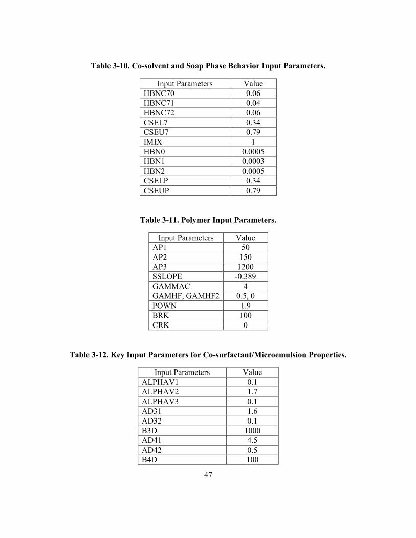
Tables 3-10, 3-11, and 3-12 summarize the key input parameters used for PCN-4

coreflood history match to represent co-surfactant and soap phase behavior, polymer and

co-solvent/microemulsion properties. Most of them are obtained from the match with the

measured lab data. For those that are not directly measured in the lab, typical values are

used and are slightly adjusted to get a good history match of oil recovery, oil cut, pressure

drop, and oil saturation curves.

0

0.1

0.2

0.3

0.4

0.5

0.6

0.7

0.8

0.9

1

0 0.1 0.2 0.3 0.4 0.5 0.6 0.7

Re

lati

ve P

erm

eab

ility

Sw

krw

kro

47

Table 3-10. Co-solvent and Soap Phase Behavior Input Parameters.


HBNC70 0.06

HBNC71 0.04

HBNC72 0.06

CSEL7 0.34

CSEU7 0.79

IMIX 1

HBN0 0.0005

HBN1 0.0003

HBN2 0.0005

CSELP 0.34

CSEUP 0.79

Table 3-11. Polymer Input Parameters.


AP1 50

AP2 150

AP3 1200

SSLOPE -0.389

GAMMAC 4

GAMHF, GAMHF2 0.5, 0

POWN 1.9

BRK 100

CRK 0

Table 3-12. Key Input Parameters for Co-surfactant/Microemulsion Properties.


ALPHAV1 0.1

ALPHAV2 1.7

ALPHAV3 0.1

AD31 1.6

AD32 0.1

B3D 1000

AD41 4.5

AD42 0.5

B4D 100

48

Figures 3-29, 3-30, and 3-31 show that UTCHEM gives a good match of

cumulative oil recovery, oil cut, and oil saturation. Simulated pressure drop in Figure 3-

32 is higher than measured experimental data, possibly due to reasons similar to what

occurred in PCN-1 coreflood (i.e. combined effects of co-solvent concentration on

microemulsion viscosity as well as shear thinning behavior of microemulsion phase). In

order to match the measured pressure drop, a higher polymer concentration, i.e. a higher

injected fluid viscosity, is required in the polymer drive. It is important to note that

waterflood was stopped after less than 0.1% change in oil cut was observed in the lab to

save the long time to reach the real residual oil saturation. Thus, for UTCHEM

simulation, initial water saturation of 0.63 at the start of ACP slug is used, instead of 0.64

as measured in the lab. The co-solvent adsorption is assumed to be zero in the simulation

model.


0%

20%

40%

60%

80%

100%

0 0.5 1 1.5 2

Cu

m O

il R

eco

vere

d, %

OO

IP

Pore Volumes

Lab

UTCHEM

49


Figure 3-31. Oil saturation for PCN-4 Coreflood.

0%

10%

20%

30%

40%

50%

60%

70%

0 0.5 1 1.5 2

Oil

Cu

t

Pore Volumes

Lab

UTCHEM

0%

5%

10%

15%

20%

25%

30%

35%

40%

0 0.5 1 1.5 2

Oil

Satu

rati

on

Pore Volumes

Lab

UTCHEM

50


3.5 SUMMARY AND CONCLUSIONS

For PCN-1 coreflood, 69.5% recovery of the waterflood residual oil saturation

was achieved and the residual oil saturation after chemical flood (Sorc) was reduced to

13.5%. The pressure drop at steady state looked reasonable with 5.5 psi across the whole

core of 1 ft length. The results seemed to be promising with very low usage of chemicals,

i.e. alkali, co-solvent and polymer. UTCHEM and CMG STARS simulations gave a good

history match of the lab measurements on cumulative oil recovery, oil cut, and oil

saturation. The higher simulated pressure drop in UTCHEM simulation than

experimental data is probably caused by the combined effects of polymer concentration

on microemulsion viscosity and shear thinning behavior of microemulsion phase. There

seems to be evidence indicating numerical instability with CMG STARS simulation in

terms of pressure drop. Adjusting the time steps and other numerical convergence input

parameters might help with the degree of oscillation.

0

2

4

6

8

10

12

14

0 0.5 1 1.5 2

Pre

ssu

re D

rop

(p

si)

Pore Volumes

Lab

UTCHEM

51

For PCN-4 coreflood, the oil recovery was 98 % of waterflood residual oil

saturation (36%) with an average oil cut of 60 % in the oil bank and the residual oil

saturation from chemical flood (Sorc) was 0.8%. The pressure drop at steady state was

measured as 12.9 psi across the 1 ft core length. Although the oil recovery of this

coreflood was very promising, the significantly increasing requirements for chemicals

hindered potential field implementation.

PCN-1 coreflood design was used for the pilot scale simulations discussed in

Chapter 4.

52

CHAPTER 4: PILOT-SCALE DESIGN OF AN ALKALINE/CO-

SOLVENT/POLYMER FLOOD

4.1 SIMULATION MODEL

The reservoir of this thesis is a sandstone reservoir at a depth of approximately

1,000 ft that has gone through waterflood for more than 5 years. The reservoir average

permeability and porosity are 2,507 md and 21% respectively. The average residual oil

saturation before ACP flood is approximately 44.3%. All geological data, e.g.

permeability, porosity, reservoir pressure, initial water saturation, gridblock thickness,

and Net-to-Gross (NTG) for each model cell were provided by the operator. The water

saturation at the start of ACP flood in UTCHEM model matched the field production data

provided by the operator.

The pilot area is approximately 419 acres and includes 6 inverted 7-spot well

patterns. The simulation model is approximately 2,458 acres with 28 pilot wells located

in the center of the grid. The reservoir model is approximately 9,711 ft × 11,024 ft × 98

ft. The gridblock size on each of the 5 layers is identical, 262.47 ft × 262.47 ft, while the

layer thickness from top to bottom is 14.58, 7.97, 10.90, 14.70 and 49.96 ft respectively.

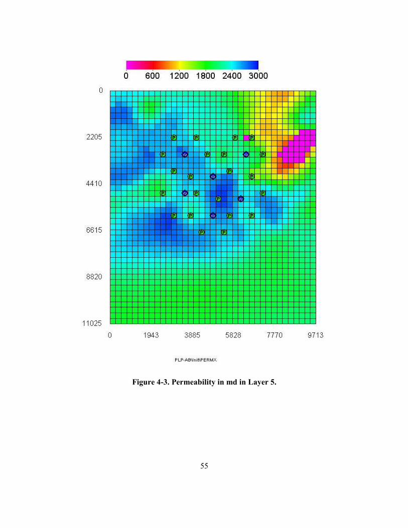
Figures 4-1, 4-2 and 4-3 are maps of the permeability distribution in the first, third and

fifth layer and also display the location of the pilot area. The oil saturation in layers 1, 3

and 5 before ACP slug are shown in Figures 4-4, 4-5 and 4-6 respectively. Table 4-1

summarizes the simulation model and fluid properties. The chemical slug was based on

the engineering design for PCN-1 coreflood.

53

Figure 4-1. Permeability in md of Layer 1.

54

Figure 4-2. Permeability in md in Layer 3.

55

Figure 4-3. Permeability in md in Layer 5.

56

Figure 4-4. Oil Saturation in Layer 1.

57


58


59

Table 4-1. List of Simulation Model Properties.

Model Size 9,711 ft ×11,024 ft × 98 ft

Grid Size

262.47 ft ×262.47 ft × 14.58 ft (Layer 1)

262.47 ft ×262.47 ft × 7.97 ft (Layer 2)

262.47 ft ×262.47 ft × 10.90 ft (Layer 3)

262.47 ft ×262.47 ft × 14.70 ft (Layer 4)

262.47 ft ×262.47 ft × 49.96 ft (Layer 5)

Average Porosity 21%

Average Permeability 2507 md

kv/kh 0.1

Initial Oil Saturation (before ACP) 44.3%

Reservoir Depth 1,000 ft

Reservoir Temperature 38 oC

Initial Pressure 500 psi

Water/Oil Relative Permeability

S1rw = 0.17; S2rw = 0.45

0r1k = 0.07; 0

r2k = 0.95

e1w = 10; e2w = 1.5

Water Viscosity

(at Reservoir Temperature) 0.534 cp

Oil Viscosity

(at Reservoir Temperature) 170 cp

Formation Brine Total Anion = 0.0158 meq/mL

Total Divalent Cation = 0.0082 meq/mL

Oil/Brine IFT 19.95 dynes/cm

60

The match of the test tube phase behavior and history match of coreflood for this

formulation was discussed in Chapter 3. The parameters obtained from the history match

were used for the base case field-scale simulation and they are listed in Table 4-2.

Table 4-2. List of Cosolvent and Polymer Parameters.

Hand’s Rule Parameters

HBNC70: 0.22

HBNC71: 0.18

HBNC72: 0.22

Optimum Salinity 0.26 meq/mL

Type III Salinity Window CSEL7: 0.2 meq/mL

CSEU7: 0.32 meq/mL

Cosolvent Retention 0.16 mg/g rock

Polymer Adsorption 7.2 µg/g rock

Microemulsion Viscosity 90 cp

Trapping Number Parameters

Water (T11) = 1,865

Oil (T22) 59,074

Microemulsion (T33) = 364.2

Relative Permeability Parameters

(at High Capillary Number) assumed miscible

Six injection wells for the inverted 7-spot pattern have constant injection rates of

1,110, 862, 1,120, 579, 1,128 and 382 BPD respectively. The bottomhole pressure varies

for 22 production wells in the pilot area for the base case simulation, ranging from 152 to

546 psi. This meets the operating conditions in the field without causing damage to the

formation or exceeding facility capacity. The flow rates of the producers would drop

significantly when viscous oil bank is produced, since the oil bank mobility is lower than

61

the mobility of the fluid with high water-cut ahead of it. Thus, all producers are set to be

pressure-constraint instead of rate-constraint, in order to capture the propagation of the

viscous oil bank and to forecast the oil recovery more accurately. If producers are rate-

constraint, the ultimate oil recovery from simulations will be over-optimistic due to

extremely high bottomhole pressure at production wells that completely exceeds the

facility capacity.

4.2 BASE CASE SIMULATION

The pilot contains six repeating inverted 7-spot well patterns. A map of the

injection and production wells is displayed in Figure 4-1, with blue markers representing

injection wells and green markers are production wells. Within the pilot area, there are 6

injectors and 22 producers. Table 4-3 briefly summarizes the injection scheme

implemented in the field and the chemical composition of ACP and polymer drive slugs.

The pilot starts with 10 years (~ 0.1 PV) of ACP flood with 1.5% cosolvent, chased by 10

years (~ 0.1 PV) of polymer drive. The UTCHEM input file for the base case pilot-scale

simulation is given in Appendix C.

62

Table 4-3. Base Case ACP Flood Design.

Injector Well Constraint 1110, 862, 1120, 579, 1128, 382 BPD

Producer Well Constraint Varies for 22 Producers (153 – 546 psi)

Pore Volume (in Pilot Area) 51,934,397 bbls

Oil-in-Place (in Pilot Area) 30,231,985 bbls

ACP Slug

10 Years

1.5 % Cosolvent

2750 ppm Polymer

Salinity = 0.1265 meq/mL

Polymer Drive

10 Years

2250 ppm Polymer


Water Postflush 10 Years


The base case simulation results (Figures 4-7 and 4-8) indicated that the pilot can

recover approximately 8,340,500 bbls of oil, which accounts for 10.885 % of the oil-in-

place before water postflush. Figures 4-9, 4-10 and 4-11 show the oil saturation at the end

of the polymer drive. Since the bottom layer is more permeable and homogeneous than

the top layer, a better volumetric sweep is observed as expected.

63

Figure 4-7. Base Case – Cumulative Oil Production.

0

1000000

2000000

3000000

4000000

5000000

6000000

7000000

8000000

9000000

0 1000 2000 3000 4000 5000 6000 7000 8000 9000 1000011000

Cu

m. O

il P

rod

uct

ion

(B

bls

)

Time (Days)

64

Figure 4-8. Base Case – Total Production Rate and Oil Cut.

0

1000

2000

3000

4000

5000

6000

7000

0

0.1

0.2

0.3

0.4

0.5

0.6

0.7

0.8

0.9

0 1000 2000 3000 4000 5000 6000 7000 8000 9000 1000011000

Tota

l Pro

du

ctio

n R

ate

(B

PD

)

Oil

Cu

t

Time (Days)

Oil Cut

Total Rate

65

Figure 4-9. Base Case – Oil Saturation after Polymer Drive (Layer 1).

66


67


4.3 SENSITIVITY SIMULATION STUDIES

The results of the base case simulation showed that the oil was mobilized and

produced from the pilot area and the oil saturation was quite uniformly reduced. The

objective of this section was to look at the impacts of difference design parameters (e.g.

68

chemical slug concentrations and sizes, polymer injection prior to ACP (PPF), injector

constraints, and well spacing) on the ultimate oil recovery and to optimize the final

engineering design with the consideration of facility capacity and field operational

conditions, chemical retention, heterogeneity, mixing and dispersion effects.

Sensitivity study with different design parameters was conducted to obtain the

optimum field-scale engineering design and to identify the effects of key uncertain

parameters. The ACP slug concentration affects the injected chemical mass and thus both

the oil recovery and the project economics. The retardation factor of the ACP slug,

defined as the loss of frontal velocity due to retention and in the units of pore volume, is

also influenced by the changes in ACP slug concentration, i.e. a lower injected chemical

concentration, a higher retardation factor. The ACP slug size might also impact the oil

recovery and project economics, since the change in ACP slug size would lead to a

change in salinity gradient (See Appendix A). A shorter ACP slug tends to have a steeper

salinity gradient than a longer slug, which could potentially negatively impact the

performance during polymer drive.

The polymer concentration provides the mobility control essential to

heterogeneous reservoirs. The polymer drive slug size affects the salinity gradient to a

lesser extent. Previous literature has reported that tapering the polymer concentration

during PD can help the project economics as well. Polymer preflush can also improve

mobility control so that the subsequent chemical slug would be more evenly distributed,

and as a result, the volumetric sweep efficiency would be significantly enhanced. Closer

well spacing could also serve for the purpose of mobility control. Due to the shorter

distance between injector and producer within the well pattern, the pore volume that

would otherwise not be accessed with larger well spacing could be swept by the chemical

slug and residual oil would be further mobilized to enhance the oil production.

69

In order to maximize the region of ultra-low interfacial tension, Pope et al. (1979)

suggested that the salinity gradient design where the formation brine salinity ahead of

chemical slug may be greater than the optimum salinity, the injected slug at optimum

salinity, and the tail of the slug at salinity lower than the optimum salinity. A detailed

economic analysis was performed to provide support to design optimization. The

economic analysis used discounted cash flow (DCF) method to calculate the net present

value (NPV) for each scenario. In order to complete the task, UTCHEM simulated

production data for each scenario was imported into CFEM, i.e. an economic model

specifically designed for chemical flooding as described in Vaskas (1996) and Wu et al.

(1996). The first step of the process was to copy the simulation data, including time, pore

volume of injected fluid, total injection rate (bbl/day), total production volume (bbl), and

total production rate (bbl/day) obtained from the well history files, into an Excel

spreadsheet called ‘CFEM.dat’ to obtain annualized data. Then the spreadsheet calculated

the annualized production data, e.g. pore volumes of injected fluids, total water injection,

and total oil and water production. The processed data was later imported into another

spreadsheet called ‘CFEM.xls’.

CFEM.xls calculated NPV using the imported simulation data with assumed

economic input parameters. The spreadsheet executed several DCF calculations to obtain

NPV, which were explained in details as following. The net revenue was calculated based

on the gross revenue (i.e. the multiplication of the oil produced during the year and the

assumed oil price of that year.) and the royalty (i.e. the percentage of the gross revenue

paid to the third parties). In other words, the net revenue was the gross revenue minus the

royalty payment. The chemical costs were the mass of chemicals injected during the year

times the chemical price of that year, while the operating costs were entered in $ per

month. The taxable income was calculated by subtracting the net revenue from the sum

70

of the chemical and operating costs. The net income was the taxable income minus the

income tax plus the EOR tax credit. Then, DCF analysis calculated the net income in

today’s dollar value by discounting the value back to the year of zero and the NPV was

calculated based on the DCF. The optimum field-scale engineering design could be

selected based on the simulation results of various scenarios with the highest NPV. The

equations used for DCF analysis were represented below (Alusta et al., 2012).

Cash Flow = Revenue – Capital Expenditure – Operating Expenditure (1)

(2)

(3)

Where (CF0) is the cash flow received in the first year, (CF1) received in the second year,

and etc. (i) is the discount rate, and the net present value index (NPVI), being the ratio

between NPV(i) and MCO(i), i.e. the Maximum Capital Outlay.

Table 4-4 listed the assumptions and input parameters used for the economic

analysis in this thesis. The capital and operating costs cover the installation of facilities

and equipment in the field, injection operating cost, chemical injection cost as well as

fluid treatment cost. The operating costs were based on the actual injection and

production volume. Co-solvent was used for this study and its price is much cheaper than

surfactant. As a readily available commercial product, the polymer price was already

known. Typical tax rates, i.e. royalty, severance and ad valorem, income tax and EOR tax

credit, for a National Oil Company (NOC) were used. A commonly-used discount rate of

10% for the oil and gas industry was also adopted for this project. It is important to note

that the assumptions made in the DCF analysis in this thesis were based on US values,

and therefore, it might not properly represent the field under study. However, the results

can provide valuable information to the operators as to further optimize the field-scale

engineering design.

71

Table 4-4. Economic Analysis Input Parameters.

Capital and Operating Costs

Equipment Cost $100,000

Operating Cost $10,000 per month

Chemical Injection Cost $0.10 per bbl

Fluid Treatment Cost $0.10 per bbl

Oil and Chemical Prices

Discounted Oil Price $50 per bbl

Alkaline Price $0.10 per lb

Co-solvent Price $0.80 per lb

Polymer Price $1.50 per lb

Taxation Rates

Royalty 15%

Severance and Ad valorem 5%

Income Tax 36.64%

EOR Tax Credit 15%

General Rates Inflation Rate 3%

Real Discount Rate 10%

4.3.1 Sensitivity to ACP Slug Size

The oil reservoir under this research on is located in a remote area of the country.

Logistics of transporting chemicals for the chemical flooding purpose from nearby city is

very expensive. ACP slug size was one important parameter investigated in this

sensitivity study. It was interesting to run pilot-scale simulations with smaller ACP slug

sizes and compare its impact on cumulative oil recovery to optimize the amount of

chemicals.

The slug size was determined based on the injection time in years and it ranged

from 3 to 10 years. The detailed description of the simulations and the summary of the

72

cumulative oil recovery for each scenario were shown in Table 4-5. The simulation of the

base case with ACP slug size of 10 years achieved the highest oil recovery, while it had

the lowest chemical efficiency ($15.95/bbl oil). The advantage of injecting larger ACP

slug to overcome the retardation factor might be offset by severe channeling due to

heterogeneity. On the other hand, the simulation which had the lowest recovery and the

least years of ACP slug injection achieved the highest chemical efficiency ($7.67/bbl oil).

Table 4-5. List of Simulations for ACP Slug Size Sensitivity.

Case

ID

ACP

Slug

Size

(yrs)

Alkaline

Conc.

(meq/mL)

Cosolvent

Conc. (vol%)

PD Slug

Size

(yrs)

Polymer Conc.

(wt%) Cum. Oil

(MMBbls) ACP PD

3-1-1 10 0.1132 1.5 10 0.275 0.225 8.3405

3-1-2 3 0.1132 1.5 10 0.275 0.225 7.2471

3-1-3 5 0.1132 1.5 10 0.275 0.225 7.6869

3-1-4 8 0.1132 1.5 10 0.275 0.225 8.1314

Table 4-16 summarized the economic analysis results for the simulations with

various ACP slug size. Assuming an oil price of $50/bbl, an alkali price of $0.10/lb, a co-

solvent of $0.80/lb and a polymer of $1.50/lb, the simulation with the smallest ACP slug

size of 3 years had the lowest NPV of $788 million. The trend of NPV as a function of

ACP slug size indicated that increasing ACP slug size leads to an increasing NPV at the

assumed oil and chemical prices. The optimum slug size was larger than 10 years (or 0.1

PV) for high oil price and low co-solvent cost.

73

4.3.2 Sensitivity to Polymer Drive Size

Polymer drive (PD)size was another important parameter to consider for this

sensitivity study, during which PD slug sized ranging from 0.06 to 0.3 PV have been

tested. Table 4-6 summarized the results of these simulations and a comparison of the

cumulative oil recoveries. The simulation with the highest oil recovery was the case with

the largest PD slug size of 0.3 PV. The trend showed that the increased amount of oil

production per increased PD slug size started to level off at 0.3 PV, possibly due to sever

channeling and permeability reduction. Even though 0.3 PV polymer slug size had the

highest oil recovery, it had the lowest chemical efficiency ($19.93/bbl oil), while the case

with the smallest PD slug size had the highest efficiency and lowest oil recovery.

Table 4-6. List of Simulations for PD Slug Size Sensitivity.

Case

ID

ACP Slug

Size (yrs)

Alkaline

Conc.

(meq/mL)

Cosolvent

Conc.

(vol%)

PD

Size

(yrs)

Polymer Conc.

(wt%) Cum. Oil

(MMBbls) ACP PD

3-2-1 10 0.1132 1.5 6 0.275 0.225 8.0587

3-2-2 10 0.1132 1.5 12 0.275 0.225 8.4096

3-2-3 10 0.1132 1.5 18 0.275 0.225 8.6305

3-2-4 10 0.1132 1.5 24 0.275 0.225 8.7671

3-2-5 10 0.1132 1.5 30 0.275 0.225 8.8860

Table 4-16 provided the economic analysis of simulations for various PD sizes.

The simulation with the highest NPV of $1,350 million was the case with 30 years of

polymer injection. An increase in PD size led to an increase in the NPV at an assumed oil

price of $50, but the marginal gain in oil recovery from increased slug size became less

with increasing slug size. The trend of NPV as a function of PD size was similar to the

74

simulations of chemical concentrations during ACP slug. The optimum PD size was

approximately 0.3 PV for higher oil price and lower co-solvent cost.

4.3.3 Sensitivity to Injection Rates

When field condition and facility capacity allows, well injection rate is the key

parameter to adjust in order to reduce the project life and increase the oil production.

Table 4-7 showed the simulation results and the comparison of oil recovery for different

injection rate. Simulations with injection rates increased to 125% and 150% of the base

case were tested. The case with the highest rates had the highest oil recovery of 9.2996

MMBbls. The case with lower rates had recoveries of 8.3405 and 8.8697 MMBbls oil

respectively.

Table 4-7. List of Simulations for Injection Rates Sensitivity.

Case

ID Description

Inj. Rate (BPD) Cum. Oil

(MMBbls) Well

1

Well

2

Well

3

Well

4

Well

5 Well 6

3-3-1 Base Case 1110 862 1120 579 1128 382 8.3405

3-3-2 125% Inj.

Rate

1387 1077 1400 723 1409 478 8.8697

3-3-3 150% Inj.

Rate

1664 1292 1680 868 1692 574 9.2996

The change in injection rates and cumulative oil recovery resulted in the

difference of chemical efficiency of the simulations. The simulation with the highest

injection rate had a lowest chemical efficiency ($21.42/bbl oil), in comparison to the base

case ($15.95/bbl oil). At the assume oil and chemical prices, therefore, the simulation

75

with the lowest well injection rates was optimum for this design parameter. Table 4-16

provided the economic analysis results for simulations of different injection rates. It

indicated that the case with the highest injection rate had the highest NPV of $1,317

million. An increase in injection rates led to an increasing NPV.

4.3.4 Sensitivity to Polymer Adsorption

The alkali, co-solvent, and polymer retentions were considered as uncertainties

and chemical efficiency. The retention values used in this section were within the typical

range. The retardation factor and the required amount of chemicals were the primary

effects of adsorption.

The polymer adsorption is highly uncertain for the reservoir. The base case

assumed 7.2 µg/g rock based on coreflood. The retardation factor for polymer would be

impacted with the change of the polymer adsorption. The change would also influence

mobility control and permeability reduction associated with the concentration. The lower

polymer adsorption led to a slightly higher oil recovery (8.3449 MMBbls). This is

probably due to the decreasing loss of polymer to the reservoir rock, and thus, a larger

amount of polymer was effective for mobility control and permeability reduction.

Nevertheless, it was safe to conclude that the oil production from this reservoir was

insensitive to polymer adsorption. These simulations only made a slight difference in

NPVs, as shown in Table 4-16. The base case gave a NPV of $1,080 million while the

case with lower or higher polymer adsorption gave a NPV of $1,087 and $1,074 million

respectively.

76

Table 4-8. List of Simulations for Polymer Adsorption Sensitivity.

Case

ID Description

Polymer Adsorption

Parameters Polymer Adsorption

(µg/g rock)

Cum. Oil

(MMBbls) AD41

AD42

(mL/meq)

3-4-1 Base Case 0.48 0.48 7.2 8.3405

3-4-2 Lower

Adsorption 0.24 0.24 3.6 8.3449

3-4-3 Higher

Adsorption 0.96 0.96 14.4 8.3334

4.3.5 Sensitivity to Alkaline Retention

The alkaline retention employed was based on coreflood history match.

Simulations were conducted for a retention value of 50% and 200% of the base case

respectively. Table 4-9 showed a comparison of the cumulative oil recovery for the

simulations of different alkaline retentions. The lower alkaline retention value gave a

higher oil recovery. The economic analysis results were shown in Table 4-16. It was

interesting to observe that the highest alkaline retention (200% of the base case value)

gave a slightly higher NPV ($1,081) than that of the base case, which was probably due

to the longer retention time of alkaline within the reservoir and the greater chance to react

with acid components of heavy oil to generate in-situ soap.

77

Table 4-9. List of Simulations for Alkaline Retention Sensitivity.

Case ID Description ALKAD

(ft3

water/meq/mL) Cum. Oil (MMBbls)

3-5-1 Base Case 5 8.3405

3-5-2 Lower Alkaline Retention 2.5 8.3491

3-5-3 Higher Alkaline Retention 10 8.3218

4.3.6 Sensitivity to Chemical Concentrations during ACP

25% and 50% fraction of the chemical concentrations during ACP slug of the

base case were tested for comparison purpose. The chemical concentrations were

theoretically directly associated with the cumulative oil recovery. The base case

simulation had an oil production of 8.3405 MMBbls whereas only 25% and and 50%of

the concentration of the base case had 7.0578 and 7.3283 MMBls oil recoveries

respectively. Table 4-10 showed the comparison of cumulative oil recovery for

simulations with various chemical concentrations.

The chemical efficiency for these simulations was different, possibly due to the

different injected chemical amount and the cumulative oil recovery. The simulation with

the lowest chemical concentrations gave a highest chemical efficiency ($7.11/bbl oil), in

comparison to the base case of the highest concentrations ($15.95/bbl oil), along with a

chemical efficiency of $10.62/bbl oil from the simulation with lower concentrations. It

was therefore apparent that at the assumed oil and chemical prices the simulation with the

lowest injected chemical concentrations was optimum for this parameter.

78

Table 4-10. List of Simulations for Chemical Conc. Sensitivity during ACP.

Case

ID Description

ACP

Slug

Size

(yrs)

Alkaline

Conc.

(meq/mL)

Cosolvent

Conc.

(vol%)

PD

Slug

Size

(yrs)

Polymer Conc.

(wt%) Cum. Oil

(MMBbls) ACP PD

3-6-1 Base Case 10 0.1132 1.5 10 0.275 0.225 8.3405

3-6-2

50%

Chemical

Conc.

10 0.0566 0.75 10 0.1375 0.225 7.3283

3-6-3

25%

Chemical

Conc.

10 0.0283 0.375 10 0.06875 0.225 7.0578

Table 4-16 showed the economic results for the simulations using various injected

chemical concentrations during ACP slug. At an oil price of $50, the simulation of the

base case had a higher NPV ($1,080 million) than those of lower chemical concentrations

($918 and $826 million respectively). At the assumed oil and chemical price, the

optimum concentrations were higher than the base case. The DCF analysis based on these

simulations indicated that the higher concentration was the optimum value, which was

opposite to the conclusions drawn from the chemical efficiency.

4.3.7 Sensitivity to Polymer Concentrations for Mobility Buffer

Polymer concentration during PD is another important parameter for mobility

control and permeability reduction during chemical flood. Injected polymer concentration

was decreased to 25% and 50% of the base case concentration for sensitivity study. Table

4-11 presented the outcome of these simulations and a comparison of the cumulative oil

79

recoveries. It showed that the oil recovery was directly associated with the injected

polymer concentration. However, it was less sensitive to changes in polymer

concentration during PD slug than to chemical concentrations during ACP slug. The base

case with the highest polymer concentration (2,250 ppm polymer for 0.1 PV) had the

highest cumulative oil recovery, but it also had the lowest chemical efficiency. The trend

was similar to the simulations of various chemical concentrations during ACP slug where

the highest concentration led to the lowest efficiency.

Table 4-11. List of Simulations with Various Polymer Conc. during Mobility Buffer.

Case

ID Description

ACP

Slug

Size

(yrs)

Alkaline

Conc.

(meq/mL)

Cosolvent

Conc.

(vol%)

PD

Size

(yrs)

Polymer Conc.

(wt%) Cum. Oil

(MMBbls) ACP PD

3-7-1 Base Case 10 0.1132 1.5 10 0.275 0.225 8.3405

3-7-2

50%

Chemical

Conc.

10 0.1132 1.5 10 0.275 0.1125 8.0940

3-7-3

25%

Chemical

Conc.

10 0.1132 1.5 10 0.275 0.05625 7.9434

Table 4-16 provided the economic results. Among these simulations, an increase

in the polymer concentration resulted in the increasing NPV. The benefits from increased

oil recovery could overcome the increasing cost of polymer and the reduction in the well

injectivity. The trend of NPV underlined the importance of mobility control in this

80

heterogeneous reservoir. The simulation with the optimum NPV of $1,080 million was

the case with 2,250 ppm polymer for 0.1 PV injected for six inverted five-spot pattern.

4.3.8 Sensitivity to Polymer Preflush (PPF)

The polymer preflush treatment has been successfully used in wells in the US.

The technique, developed in 1995, involves an in-situ generated polymer conformance

system that reduces water flow by decreasing the formation permeability to water. It does

not shut off water flow. Instead, it disproportionately reduces the formation effective

permeability to water. The permeability reduction lessens water flow without

significantly impairing hydrocarbon production. Have a PPF treatment ahead of ACP

slug injection would provide better mobility control for the injected chemicals as well as

increase the volumetric sweep efficiency so that more residual oil would be mobilized

and oil production in theory could be significantly enhanced.

The PPF size, as another key design parameter important for mobility control

during the chemical flood, was tested. Compared to the base case, simulations were run

with increased PPF sizes. Table 4-12 showed the simulation results and a comparison of

the cumulative oil recoveries for the simulations. It suggested that the oil recovery was

directly related to the size of PPF. The simulation with the largest PPF ssize (5 years for

0.05 PV) had the highest cumulative oil recovery, but it also gave the worst chemical

efficiency.

81

Table 4-12. List of Simulations for Polymer Preflush Slug Size Sensitivity.

Case

ID Description

PPF

Size

(yrs)

ACP

Slug

Size

(yrs)

Alkaline

Conc.

(meq/mL)

Cosolvent

Conc.

(vol%)

PDSize

(yrs)

Polymer

Conc. (wt%) Cum. Oil

(MMBbls) ACP PD

3-8-

1

Base Case

(0 yr PPF) 0 10 0.1132 1.5 10 0.275 0.225 8.3405

3-8-

2 1 yr PPF 1 10 0.1132 1.5 10 0.275 0.225 8.4036

3-8-

3 2 yr PPF 2 10 0.1132 1.5 10 0.275 0.225 8.4547

3-8-

4 3 yr PPF 3 10 0.1132 1.5 10 0.275 0.225 8.5003

3-8-

5 4 yr PPF 4 10 0.1132 1.5 10 0.275 0.225 8.5412

3-8-

6 5 yr PPF 5 10 0.1132 1.5 10 0.275 0.225 8.5779

Table 4-16 provided the economic analysis results for simulations of various PPF

slug sizes. Among these simulations, NPV was directly associated with the PPF slug size.

The case with the largest PPF slug size (0.05 PV) gave the highest NPV of $1,151. The

trend underscored the significance of mobility control in this heterogeneous reservoir. It

was expected that after exceeding certain slug size the cost of polymer and the reduction

in the well injectivity would begin affecting the project economics regardless of the

increased oil recovery. However, this phenomenon was not captured within this study.

82

4.3.9 Sensitivity to Pressure Constraint Injectors

It was discussed in the previous section that higher well injection rates would lead

to a higher cumulative oil recovery and NPV but a relatively lower chemical efficiency.

In order to maintain constant injection rates throughout ACP and PD slug, some of the

injection wells might experience high operating pressure due to the heterogeneity of the

reservoir, which might adversely impact the facility and the project economics. In this

section, injection wells with a constant pressure constraint were tested to better take

advantage of the mobility control and permeability reduction. Table 4-13 showed the

simulation results and a comparison of the cumulative oil recoveries. The trend suggested

that injection pressure constraint is directly associated with the oil recovery. Figures 4-12

− 4-17 presented the injection rates of the case with a constant pressure constraint of

5,000 psi for each individual well. Most of the wells gave injection rates higher than the

constant designed rates, since the wellbore around certain injection wells might be very

permeable and a larger amount of chemicals could be injected to achieve better interfacial

tension reduction and mobility control. As a consequence, more pore volume would be

swept and additional residual oil would be mobilized.

Table 4-16 provides the chemical efficiency and NPV for each simulation. The

simulation with the highest pressure constraint (5,000 psi) gave the worst chemical

efficiency of $17.85/bbl oil whereas the case with the lowest pressure constraint (1,000

psi) gave the best efficiency of $4.13/bbl oil. On the other hand, the case with 5,000 psi

constraint had the highest NPV of $1,128 million compared to $382 from the case with

1,000 psi constraint.

83

Table 4-13. List of Simulations for Pressure Constraint Sensitivity.

Case

ID Injection Well

Total Injection Rate

(ft3/day)

Cum. Oil

(MMBbls)

3-9-1 Base Case (Rate

Constraint) 29,086 8.3405

3-9-2 1000 psi BHP Constraint 8,443 4.0889



3-9-5 2500 psi BHP 14,235 6.1843

3-9-6 3000 psi BHP 18,951 6.8824

3-9-7 3500 psi BHP 24,502 7.5149

3-9-8 4000 psi BHP 31,099 8.0675

3-9-9 4500 psi BHP 38,966 8.5492

3-9-10 5000 psi BHP 48,369 8.9931

84

Figure 4-12. Injection Rate of Well 1 with 5,000 psi BHP.

85


86


87


88


89


4.3.10 Polymer Flooding (PF)

In this section, the cumulative oil recovery, chemical efficiency, and NPV were

compared between the base case ACP and the case with 20 year (0.2 PV) of polymer

flooding (1000 ppm). Table 4-14 presented the simulation results and Figure 4-18

showed a comparison of the cumulative oil recoveries. The simulation with ACP and PD

gave a higher oil recovery (8.3405 MMBbls) than the case with polymer flooding only

(6.4639 MMBbls). The disadvantage of only polymer flood with lower concentration was

the reduced level of mobility control and the aid of in-situ generated soap that lowered

the interfacial tension to mobilize additional residual oil. However, it had better chemical

efficiency due to the significantly decreasing amount of injected chemicals. Table 4-16

showed the economic analysis results for the simulations of ACP and polymer flood. The

90

case with only polymer flood gave a NPV of ($861 million) while the chase with ACP

flood gave a much higher NPV of ($1,080 million). This suggested the benefits of

interfacial tension reduction and mobility control.

Table 4-14. List of Polymer Flood Simulations.

Case

ID Description

ACP

Slug

Size

(yrs)

Alkaline

Conc.

(meq/mL)

Cosolvent

Conc.

(vol%)

PD

Size

(yrs)

Polymer Conc.

(wt%) Cum. Oil

(MMBbls) ACP PD

3-10-

1

Base Case

(10 yrs

ACP + 30

yrs PD)

10 0.1132 1.5 10 0.275 0.225 8.3405

3-10-

2 40 yrs PF 0 0 0 20 0 0.1 6.4639

91

Figure 4-18. Cumulative Oil Production of ACP + PD vs. Polymer Flood.

4.3.11 Sensitivity to Well Spacing

Well spacing affects the rate and the time at which a chemical slug can displace

oil from a reservoir. Increased well density is required to maintain a specific rate,

especially for high viscosity oil, which leads to higher process costs. The displacement

rates would decrease or the well density would increase when the oil viscosity increases.

Increasing the viscosities of the chemical slug would help to achieve mobility control

during ACP flood process. It has been known from laboratory tests that the cumulative

oil recovery via ACP flood is a function of the displacement rates. Healy et al. (1975)

showed that oil recovery was improved with an average displacement rate of 5 ft per day

compared to 1 ft per day. The Marathon-ERDA commercial demonstration test by

Marathon Oil Company (1977) presented the rate effects in the field size patterns.

0

1000000

2000000

3000000

4000000

5000000

6000000

7000000

8000000

9000000

10000000

0 3000 6000 9000 12000 15000

Cu

m. O

il P

rod

uct

ion

(B

bls

)

Time (Days)

ACP + PD

PF

92

Increasing well spacing would reduce the costs in producing wells by a margin that

allows large reservoir project to be economically feasible.

In this section, the gridblock size in x and y direction and well radius was

reduced to 25% and 50% of that of the base case and the gridblock thickness was

maintained the same. Meantime, in order to keep the same frontal velocity of the injected

slug as designed in the laboratory, the injection rate was reduced to 6.25% and 25% of

the base case respectively. All the other operating parameters were the same as the base

case. This was a quick way to investigate the impact of the well spacing on the oil

recovery. However, if a detailed economic analysis needs to be performed in the future,

the model needs to be re-constructed with new well locations and smaller well patterns.

Table 4-15 gives the parameters for various well spacing and Figure 4-19 provided a

comparison of the cumulative oil recoveries. Figure 4-20 – Figure 4-23 demonstrated the

oil saturation of layer 1 and 5 for the case of 3-12-1 and 3-12-2 respectively. The results

suggested that the smallest well patterns gave the highest oil recovery of 31.109% OOIP

compared with 11.597% from the base case. It would be quite incentive to construct

injection and production wells closer to each other to improve the mobility control of the

chemical slug, so that larger pore volume could be swept and more residual oil could be

displaced from the reservoir. Since these simulations had different amount of oil to start

with due to the difference in total pore volume, a detailed economic analysis was not

performed to determine NPV for each simulation.

93

Table 4-15. List of Simulations for Well Spacing Sensitivity.

Case

ID Description dx (ft) dy (ft)

Well

Radius (ft)

Total Injection

Rate (BPD)

Cum. Oil

(%)

3-12-1 Base Case 262.47 262.47 0.5 5180 11.597

3-12-2

50% Gridblock

Size in X, Y

Direction

131.235 131.235 0.25 1295 14.304

3-12-3

25% Gridblock

Size in X, Y

Direction

65.6175 65.6175 0.125 324 31.109

94

Figure 4-19. Cumulative Oil Recovery for Various Well Spacing.

0

5

10

15

20

25

30

35

40

0 3000 6000 9000 12000 15000

Cu

m. O

il R

eco

very

, %O

OIP

Injected PV

100% Gridblock Size

50% Gridblock Size

25% Gridblock Size

95

Figure 4-20. Oil Saturation of Layer 1 at the End of ACP Flood of Case 3-12-1 (Base

Case).

96

Figure 4-21. Oil Saturation of Layer 5 at the End of ACP Flood of Case 3-12-1 (Base

Case).

97

Figure 4-22. Oil Saturation of Layer 1 at the End of ACP Flood of Case 3-12-3 (25%

Well Spacing).

98

Figure 4-23. Oil Saturation of Layer 5 at the End of ACP Flood of Case 3-12-3 (25%

Well Spacing).

99

Table 4-16. Sensitivity Simulation Economic Analysis.

Case ID Sensitivity Variable Alkaline

Efficiency

(lb/bbl oil)

Co-solvent

Efficiency

(lb/bbl oil)

Polymer

Efficiency

(lb/bbl oil)

Chemical

Cost

($/bbl oil)

Economic

Limit

(yrs)

NPV

(MM$)

3-1-1 Base Case 4.59 11.89 3.99 15.95 20 1,080

3-1-2 ACP Slug 1.58 4.09 2.83 7.67 13 789

3-1-3 ACP Slug 2.49 6.44 3.14 10.11 15 894

3-1-4 ACP Slug 3.76 9.75 3.64 13.64 18 1,017

3-2-1 Polymer Slug 4.75 12.31 3.32 15.31 16 942

3-2-2 Polymer Slug 4.55 11.79 4.21 16.20 22 1,136

3-2-3 Polymer Slug 4.43 11.49 5.18 17.41 28 1,249

3-2-4 Polymer Slug 4.36 11.31 6.08 18.61 34 1,313

3-2-5 Polymer Slug 4.31 11.16 7.05 19.93 40 1,350

3-3-2 Injection Rate 5.39 13.98 4.66 18.72 20 1,209

3-3-3 Injection Rate 6.38 16.00 5.32 2142 20 1,317

3-4-2 Polymer Ads. 4.58 11.88 3.98 15.94 20 1,087

100

Table 4-16. Cont.

3-4-3 Polymer Ads. 4.59 11.90 3.99 15.96 20 1,074

3-5-2 Alkaline Ads. 4.58 11.88 3.98 15.93 20 1,084

3-5-3 Alkaline Ads. 4.60 11.92 3.99 15.99 20 1,081

3-6-2 ACP Conc. 2.61 6.77 3.30 10.62 20 918

3-6-3 ACP Conc. 1.36 3.51 2.58 7.11 20 826

3-7-2 Polymer Conc. 4.73 12.25 3.18 15.04 20 1,078

3-7-3 Polymer Conc. 4.82 12.49 2.76 14.61 20 1,074

3-8-2 PPF 4.56 11.80 4.13 16.10 21 1,098

3-8-3 PPF 4.55 11.73 4.28 16.27 22 1,113

3-8-4 PPF 4.54 11.67 4.44 16.44 23 1,127

3-8-5 PPF 4.54 11.61 4.59 16.63 24 1,140

3-8-6 PPF 4.54 11.56 4.74 16.82 25 1,151

3-9-2 Well Constraint 1.93 3.03 1.01 4.13 20 382

3-9-3 Well Constraint 2.10 4.36 1.54 6.00 20 448

3-9-4 Well Constraint 2.33 5.40 1.97 7.51 20 536

3-9-5 Well Constraint 2.59 6.31 2.35 8.83 20 634

101

Table 4-16. Cont.

3-9-6 Well Constraint 2.93 7.26 2.76 10.24 20 738

3-9-7 Well Constraint 3.33 8.31 3.20 11.78 20 843

3-9-8 Well Constraint 3.80 9.49 3.72 13.55 20 943

3-9-9 Well Constraint 4.34 10.83 4.32 15.58 20 1,037

3-9-10 Well Constraint 4.93 12.31 5.01 17.85 20 1,128

3-10-2 Polymer Flood 0 0 2.07 3.11 20 861

3-11-2 Co-solvent

retention

4.59 11.90 3.99 15.96 20 1,082

3-12-1 Polymer Preflush 3.98 9.95 2.95 12.78 19 1,062

3-12-2 PPF + PWF 3.88 9.68 3.41 13.24 22 1,117

102

4.4 DETERMINATION OF THE OPTIMUM ACP DESIGN

Based on the sensitivity study results, an optimum field-scale engineering design

can be then determined. With the assumed oil and chemical prices, the highest NPV for

the simulations was having a larger ACP and PD slug sizes. The relatively higher

chemical concentrations during ACP and PD slug also contributed to higher NPVs.

However, assumptions cannot be made that changing slug size and chemical

concentrations of ACP and PD all together would optimize the chemical flood result.

There was also a strong influence of well spacing on the cumulative oil recovery. Smaller

well patterns would result in higher oil recovery and most likely higher NPV. Higher well

injection rates were also directly related to oil recovery and NPV. An appropriate slug

size of polymer preflush injection, taking advantage of mobility control and permeability

reduction, also attributed to higher NPV. Last but not least, the lower values of alkaline,

co-solvent and polymer retention gave a higher NPV value.

4.5 SUMMARY AND CONCLUSIONS

The simulation model for this thesis was based on a water-wet sandstone

reservoir. The oil field has undergone a number of years of waterflood and is currently

producing high water cut. The relatively high remaining oil saturation makes the field a

promising candidate for Chemical EOR process. The reservoir and fluid properties were

transferred from CMG IMEX model provided by the field operator and a simulation

model for UTCHEM was developed accordingly.

The base case model was constructed based on the laboratory coreflood design

and scale up to the field. The simulation gave a cumulative oil recovery of 8.3405

MMBbls with promising NPV. It is important to note that the assumptions made in the

DCF analysis were based on US market values, and therefore, it might not properly

103

represent the field under study in this thesis. However, the results gave valuable

information and directions to the operators as to further optimize the field-scale

engineering design. The sensitivity study was performed to optimize the ACP flood

design. The chemical concentrations and slug sizes of ACP and PD slug were among the

key parameters studied. Increasing chemical concentration and slug sizes led to higher

cumulative oil recovery. Yet the economic analysis results showed the opposite trend for

these simulations. Other uncertain parameters, e.g. alkaline, co-solvent and polymer

retention were also studied. It showed that ACP flood for this reservoir would be

profitable even with viscous oil. At the assumed oil and chemical prices, the economic

analysis results suggested that larger slug sizes and higher chemical concentrations

during ACP and PD slug were optimum. Meantime, the fact that high NPVs could be

achieved for almost all simulations suggested that chemical flooding might be readily

feasible for this reservoir and a number of design parameters need to be studied in more

details.

The sensitivity study presented in this thesis was performed in a timely manner.

Given the time constraints, a limited number of design parameters were tested and

simulations were run. It would be more beneficial to us to investigate the impact of other

parameters on the cumulative oil recovery and project economics, including phase

behavior, grid refinement and more in-depth well spacing. Reservoir heterogeneity and

well constraints were the parameters need to be paid attention to when making chemical

flood engineering design for the field. They might adversely affect the performance of

chemical flood.

104

CHAPTER 5: SUMMARY AND CONCLUSIONS

Chemical Enhanced Oil Recovery has become more popular due to the current

high oil price and the depletion of conventional oil reservoirs. A large number of field-

scale chemical flood have been reported successful since the 1970s, a few of which are

documented in Chapter 2. Due to the combined effects of heterogeneity, facility capacity,

chemical retention, mixing and dispersion effects, the chemical flood process is far more

complex than a waterflood, and therefore, a detailed engineering design is needed for a

successful pilot- or field-scale implementation. In this thesis, UTCHEM, an in-house

chemical flood reservoir simulator, is extensively used to identify uncertain parameters

and to optimize design to significantly improve oil production and ultimately reduce

project risks.

An Alkaline/Co-solvent/Polymer (ACP) coreflood performed on a sandstone rock

was described in Chapter 3. In-situ soap formed from reaction of alkali and acid in heavy

oil significantly decreases the interfacial tension (IFT). Co-solvent improves the

compatibility between in-situ soap and polymer and has minimum rock adsorption

compare to surfactant. Polymer offers a good mobility control to drive chemical slug and

oil bank. The recovery for this coreflood was 69.5% of residual oil saturation after

waterflood and residual oil saturation from ACP flood (Sorc) was 13.5%. The pressure

drop at steady-state looked reasonable with 5.5 psi across the whole core of 1 ft length.

The result was not great, but seemed to be promising with very low usage of chemicals.

UTCHEM history matched the experimental coreflood results and obtained key model

parameters that describe phase behavior and polymer properties, and can be used for

field-scale chemical flooding simulations.

105

The pilot-scale design optimization of an ACP flood was presented in Chapter 4.

The impacts of chemical slug concentrations and sizes, polymer preflush (PPF), injector

constraints, and well spacing on oil recovery for a sandstone reservoir were greatly

studied. It was observed that high concentration chemical slugs with good mobility

control significantly benefit the project economics. The in-situ soap and injected polymer

are more compatible with the addition of co-solvent in the chemical slug. The soap not

only further mobilizes residual oil to enhance oil recovery, but also improves relative

permeability of water and oil to increase injectivity. It will also be beneficial to perform

polymer preflush before ACP slug injection to improve mobility control, to maximize

well injectivity and to ensure proper chemical slug propagation within the reservoir. It is

more exciting to notice that closer well spacing significantly spikes the oil production as

a result of greater mobility control and volumetric sweep efficiency it provided.

106

Appendix A: Salinity Gradient

Hirasaki et al. (1983) proposed that salinity gradient is critical for the success of

any surfactant process and is used to keep as much surfactant as possible in the active

region, to minimize surfactant retention, and to control the phase environments of the

surfactant slug and polymer drive. The ideal design is to have over-optimum reservoir

salinity ahead of the surfactant or alkali bank at optimum salinity and the polymer drive

at under-optimum salinity. The salinity gradient will become unfavorable when the

reservoir salinity is initially under-optimum, since the reaction and dilution effects of

injected alkali would cause the surfactant slug to be under-optimum. Additionally,

uncertainties in reservoir conditions would lead to changes to the phase behavior or to the

Type III salinity window as what has been design in the laboratory. With the unfavorable

salinity gradient, the low-IFT Type III salinity window might not be reached. It is

therefore important to have the right salinity gradient design to ensure the Type III region

for the surfactant process.

107

Appendix B: Input File of CMG STARS Model for PCN-1 Coreflood

** Test and illustrate Alkaline Surfactant Polymer flood

** =========================================================

INPUT/OUTPUT CONTROL

====================================================

RESULTS SIMULATOR STARS

*INTERRUPT *STOP

*TITLE1 'STARS Geochem Model Template #004'

*TITLE2 'ASP flood in core with adsorption'

*INUNIT *SI

*OUTUNIT *SI

WSRF WELL 1

WSRF GRID TIME

WSRF SECTOR TIME

OUTSRF GRID ADSORP PPM ADSPCMP CAPN IFT KRO KRW LOGIFT

MASDENO MASDENW MOLDENO MOLDENW

PRES RFO RFW SG SO SW TEMP VELOCRC VISO VISW W

X

*WSRF *SECTOR *TIME

*OUTPRN *WELL *ALL

*OUTPRN *ITER *UNCONV

*OUTSRF *WELL DOWNHOLE COMPONENT ALL

108

*WSRF *GRID 1

*WRST 500

*WPRN *GRID 500

*WPRN *ITER 1

** ========================================================

GRID AND RESERVOIR DEFINITION

=======================================================

*GRID *CART 1 1 100 ** One-dimensional grid

*DK *CON 0.00296

*DJ *CON 0.044345

*DI *CON 0.044345

*POR *CON 0.21 ** POROSITY

*PERMI *CON 2507 ** Permeability

*PERMJ *EQUALSI ** EQUAL TO I DIRECTION VALUE

*PERMK *EQUALSI ** EQUAL TO I DIRECTION VALUE

*END-GRID

*CPOR 1.e-4 ** SIGNALS INPUT OF ROCK COMPRESSIBILITIES

*PRPOR 101.1 ** SIGNALS INPUT OF REF PRESSURE FOR ROCK

COMPRESSIBILITIES

** ========================================================

FLUID DEFINITIONS

===============================================================

======

MODEL 5 5 5 4

109

*COMPNAME 'H2O' 'Polymer' 'Surfact' 'Alkaline'

'Dead_Oil'

** ------- ------- -------- --------- ---------

*CMM 0.018 8 0.71 0.04 0.288

** Molecular weight IN SI UNITS (Kg/gmol)

*PCRIT 0 0 0 0 0

** Critical pressure in kPa

*TCRIT 0 0 0 0 0

** Critical temperature in deg C

*MOLDEN 0 0 0 0 869.2

** Molar Density (gmol/m3)

*AVISC 0.534 100 0.534 0.534 170

** Assigned liq. viscosity

*BVISC 0 0 0 0 0

*******************************Liquid-liquid K Value

tables*******************************************************************

*************

LIQLIQKV **Assign K values in table

form. Liquid-liquid K values must be assigned this way

** Low pressure High pressure Low Temperature High

Temperature

** ----------- ------------- --------------- ----------------

110

KVTABLIM 80 100000 10

500

KVKEYCOMP 'Alkaline' W 0 0.000901991 **Name of key

component, X-low, X-high

KVTABLE 'Surfact'

KEYCOMP ** K-value table at low compostion of zero

[K(Tlow,Plow), K(Tlow,Phigh), K(Thigh,Plow), K(Thigh,Phigh)]

0 0

0 0

KEYCOMP ** K-value table at high compostion of 0.000901991

[K(Tlow,Plow), K(Tlow,Phigh), K(Thigh,Plow), K(Thigh,Phigh)]

200 200

200 200

*************************************Reaction

specification*************************************************************

********************

**-------------- Reaction specification for Polymer degradation---------------------------------

-----------

STOREAC ** Stoichiometric coefficient of reacting component

0 1 0 0 0

STOPROD ** Stoichiometric coefficient of produced component

443.951 0 0 0 0

RPHASE ** Flag defining phase for reacting component. The allowed

range is 0 to 4.(1 for Water phase, 2 for Oil phase, 3 for Gas phase)

0 1 0 0 0

111

RORDER ** Order of reaction with respect to each reacting

component's concentration factor. It must be non-negative.

0 1 0 0 0

FREQFAC 0.02284 ** Reaction frequency factor (unit is variable). It must be

non-negative.

** This is the constant factor in the expression for reaction rate.

**For chemical reactions (e.g.,combustion) Ea is positive, that is, the reaction rate

increases with increasing T.

**Reaction rate is independent of T when EACT = 0.

EACT 0 ** Single activation energy Ea (J/gmol | Btu/lbmol) gives the

dependence of reaction rate on grid block temperature.

**------------- Reaction specification for Soap generation----------------------------------------

-----------

STOREAC ** Stoichiometric coefficient of reacting component

0 0 1 1 0

STOPROD ** Stoichiometric coefficient of produced component

0 0 0 1 1

RPHASE ** Flag defining phase for reacting component. The

allowed range is 0 to 4.(1 for Water phase, 2 for Oil phase, 3 for Gas phase)

112

0 0 1 1 0

RORDER ** Order of reaction with respect to each reacting

component's concentration factor. It must be non-negative.

0 0 1 2 0

FREQFAC 0.6512 ** Reaction frequency factor (unit is variable). It must be

non-negative.

** This is the constant factor in the expression for reaction rate.

**For chemical reactions (e.g.,combustion) Ea is positive, that is, the reaction rate

increases with increasing T.

**Reaction rate is independent of T when EACT = 0.

EACT 0 ** Single activation energy Ea (J/gmol | Btu/lbmol) gives the

dependence of reaction rate on grid block temperature.

**=================================== polymer and surfactant properties

can be investigated further

======================================================

*VSMIXCOMP 'Polymer'

113

*VSMIXENDP 0 0.000609957

**----------------------------------------------- polymer viscosity dependency on shear effect

-------------------------------------------

*SHEARTAB

1.3E-04 2006.87

2.3E-04 1963.27

4.0E-04 1877.09

7.2E-04 1717.73

1.3E-03 1456.43

2.3E-03 1102.15

4.0E-03 728.00

7.2E-03 424.02

1.3E-02 225.42

2.3E-02 113.47

4.0E-02 55.57

7.2E-02 26.95

1.3E-01 13.12

2.3E-01 6.51

4.0E-01 3.36

7.2E-01 1.87

1.3E+00 1.17

2.3E+00 0.83

4.0E+00 0.68

114

**----------------------------------------------- Flopaam 3330S polymer viscosity dependency

on polymer concentration ----------------------

**Fit of nonlinear curve to nonlinear viscosity mixing function

*VSMIXFUNC 0 0.416042577 0.541608946 0.632223325 0.70660

0.770469371 0.82655922 0.876542648 0.921575374 0.962510208 1

*PRSR 101.1

*TEMR 38

*PSURF 101.1

*TSURF 38

** ===================================================== ROCK-

FLUID PROPERTIES

===============================================================

=========

ROCKFLUID

115

**----------------------------------------------- Interfacial Tension table for Surfactant --------

------------------------------------------------------

INTCOMP 'Surfact' *WATER

IFTTABLE ************************ Define Interfacial tension and

interpolation functions *****************************

**-------------------------------------------------------------------------------------------------

2CMPW 0 ** Concentration value of second component affecting the

Interfacial tension versus composition value table for component *INTCOMP

** Composition of component/phase given by *INTCOMP

Interfacial tension

0 23.4

4.960710954e-005 18.2

**-------------------------------------------------------------------------------------------------

2CMPW 0.000225312 ** Concentration value of second component affecting

the Interfacial tension versus composition value table for component *INTCOMP


Interfacial tension

0 18.21

116

4.960710954e-005 0.5

**-------------------------------------------------------------------------------------------------




Interfacial tension

0 15.54

4.960710954e-005

0.028

**-------------------------------------------------------------------------------------------------




Interfacial tension

0 12.21

4.960710954e-005

0.028

**-------------------------------------------------------------------------------------------------



117


Interfacial tension

0 7.25

4.960710954e-005 0.04

**-------------------------------------------------------------------------------------------------




Interfacial tension

0 5.023

4.960710954e-005

0.062

**-------------------------------------------------------------------------------------------------




Interfacial tension

0 4.535

4.960710954e-005

0.087

118

**-------------------------------------------------------------------------------------------------




Interfacial tension

0 5.12

4.960710954e-005 0.5

**-------------------------------------------------------------------------------------------------

INTLOG ** Logarithmic interpolation is used when doing a table lookup of

composition values vs interfacial tension.

********************************************** Relative Permeability data

***********************************************

RPT 1 WATWET ** Define rock type number for rock-fluid data, and

assign rock type number to grid blocks.(WATWET assigns for water-wet rock)

**---------------------------------------------------------------------------

KRINTRP 1 ** Relative permeability data at low capillary number

119

DTRAPW -10 ** Value of wetting phase interpolation parameter for current

rock-fluid data set

DTRAPN -3 ** Value of non-wetting phase interpolation parameter for current

rock-fluid data set

** Sw krw krow

SWT

0.17 0 0.95

0.18 6.44494E-20 0.916074692

0.19 6.59962E-17 0.882966822

0.2 3.80567E-15 0.850666419

0.21 6.75801E-14 0.819163517

0.22 6.29389E-13 0.788448146

0.23 3.89701E-12 0.758510337

0.24 1.82054E-11 0.729340121

0.25 6.9202E-11 0.700927531

0.26 2.24721E-10 0.673262596

0.27 6.44494E-10 0.646335349

0.28 1.67165E-09 0.62013582

0.29 3.99054E-09 0.594654041

0.3 8.8849E-09 0.569880043

0.31 1.86423E-08 0.545803857

0.32 3.71648E-08 0.522415515

0.33 7.08629E-08 0.499705048

120

0.34 1.2993E-07 0.477662486

0.35 2.30115E-07 0.456277862

0.36 3.95144E-07 0.435541207

0.37 6.59962E-07 0.415442551

0.38 1.07501E-06 0.395971927

0.39 1.71177E-06 0.377119364

0.4 2.66992E-06 0.358874896

0.41 4.08631E-06 0.341228552

0.42 6.14638E-06 0.324170364

0.43 9.09814E-06 0.307690364

0.44 1.32696E-05 0.291778582

0.45 1.90897E-05 0.27642505

0.46 2.71143E-05 0.261619799

0.47 3.80567E-05 0.24735286

0.48 5.28246E-05 0.233614265

0.49 7.25636E-05 0.220394045

0.5 9.87094E-05 0.207682231

0.51 0.000133048 0.195468855

0.52 0.000177787 0.183743947

0.53 0.000235637 0.172497538

0.54 0.000309911 0.161719661

0.55 0.000404627 0.151400347

0.56 0.000524645 0.141529626

0.57 0.000675801 0.132097529

0.58 0.000865083 0.123094089

121

0.59 0.001100809 0.114509337

0.6 0.001392848 0.106333302

0.61 0.001752854 0.098556018

0.62 0.002194544 0.091167515

0.63 0.002733993 0.084157825

0.64 0.003389984 0.077516977

0.65 0.004184383 0.071235005

0.66 0.005142566 0.065301939

0.67 0.00629389 0.059707811

0.68 0.007672216 0.054442651

0.69 0.009316494 0.049496491

0.7 0.011271398 0.044859362

0.71 0.013588036 0.040521296

0.72 0.016324729 0.036472323

0.73 0.019547866 0.032702475

0.74 0.023332842 0.029201783

0.75 0.027765085 0.025960279

0.76 0.032941183 0.022967993

0.77 0.038970105 0.020214958

0.78 0.045974544 0.017691203

0.79 0.054092365 0.015386761

0.8 0.063478195 0.013291663

0.81 0.074305133 0.011395939

0.82 0.086766613 0.009689622

0.83 0.101078417 0.008162742

122

0.84 0.117480856 0.006805331

0.85 0.136241119 0.00560742

0.86 0.157655811 0.00455904

0.87 0.182053686 0.003650223

0.88 0.209798589 0.002870999

0.89 0.241292621 0.0022114

0.9 0.276979532 0.001661458

0.91 0.317348371 0.001211203

0.92 0.362937389 0.000850666

0.93 0.414338223 0.00056988

0.94 0.472200375 0.000358875

0.95 0.537235995 0.000207682

0.96 0.61022499 0.000106333

0.97 0.692020478 4.48594E-05

0.98 0.783554601 1.32917E-05

0.99 0.885844718 1.66146E-06

1 1 0

**---------------------------------------------------------------------------

KRINTRP 2 ** Relative permeability data at high capillary number

DTRAPW -1

DTRAPN -1

** Sw krw krow

SWT

123

0.17 0 1

1 1 0

*********************************** Adsorption Data, Permeability reduction

and inaccessible pore volume data for Polymer ******************************

**---------------------------- Data for irreversible aqueous polymer adsorption ---------

--------------------------------------

*ADSCOMP 'Polymer' WATER

*ADMAXT 0

*ADRT 0

**---------------------------- Permeability Reduction-Inaccessible pore volume

parameters------------------------------------------

*RRFT 1

*PORFT 0.93

**-------------------------- Langmuir concentration coefficients for adsorption equation-----

----------------------------------------

*ADSLANG 0 0 1.0E-15

124

** ======================================================

INITIAL CONDITIONS

===============================================================

============

*INITIAL

*PRES *CON 101.1 **set const pressure of 101.1 kPa

*SW *CON 0.557

*SO *CON 0.443

*TEMP *CON 38

**$ Property: Water Mole Fraction(H2O) Max: 1 Min: 1

*MFRAC_WAT 'H2O' CON 1

*MFRAC_OIL 'Dead_Oil' CON 1

** ======================================================

NUMERICAL CONTROL

===============================================================

==============

*NUMERICAL

125

*ITERMAX 100

*DTMAX .025 ** change max time step to .025 days in lab

*TFORM *ZT

*ISOTHERMAL

*NORM *PRESS 150 *ZO .2 *TEMP 38 *ZNCG .2 *ZAQ .2

** =======================================================

RECURRENT DATA

===============================================================

=============

*RUN

*TIME 0

*DTWELL 0.0025

**---------------------------------------------------

WELL 'INJTR'

** well radius Geometric factor for the well Fraction of a circle

that the well model Skin factor

GEOMETRY K 0.000914 0.249

1 0

126

PERF TUBE-END 'INJTR'

** UBA ff Status Connection

1 1 1 1.1 OPEN FLOW-FROM 'SURFACE'

**---------------------------------------------------

WELL 'PRODN'

PRODUCER 'PRODN'

OPERATE MIN BHP 101.1 CONT

** well radius Geometric factor for the well Fraction of a circle

that the well model Skin factor

GEOMETRY K 0.000914 0.249

1 0

PERF TUBE-END 'PRODN'

** UBA ff Status Connection

1 1 100 1 OPEN FLOW-TO 'SURFACE'

**-------------------------------------ASP Flood Step------------------------------------------------

-

INJECTOR UNWEIGHT 'INJTR'

127

**COMPNAME 'H2O' 'Polymer' 'Surfact' 'Alkaline'

'Dead_Oil'

INCOMP WATER 0.971001526 0.000609957 0.000374877 0.02801364

0.

*OPERATE *STW 0.000126 ** .11mL/min reported in paper converted to m3/day

*TIME 0.02914

*TIME 0.058274

*TIME 0.087409

*TIME 0.11654

*TIME 0.14568

*TIME 0.17481

*TIME 0.20395

*TIME 0.23308

*TIME 0.26222

*TIME 0.29135

*TIME 0.32048

*TIME 0.34962

*TIME 0.37875

*TIME 0.40789

*TIME 0.43702

*TIME 0.46616

*TIME 0.485606815 ** 0.5 PV ASP

128

*DTWELL 0.0025

**-------------------------------------Polymerflood Step---------------------------------------------

----

WELL 'INJTR'

INJECTOR UNWEIGHT 'INJTR'

**COMPNAME 'H2O' 'Polymer' 'Surfact' 'Alkaline'

'Dead_Oil'

INCOMP WATER 0.999494006 0.000505994 0. 0.

0.

*OPERATE *STW 0.000126 ** .11mL/min reported in paper converted to m3/day

*TIME 0.51485

*TIME 0.54399

*TIME 0.57312

*TIME 0.60226

*TIME 0.63139

*TIME 0.66052

*TIME 0.68966

*TIME 0.71879

*TIME 0.74793

*TIME 0.77706

129

*TIME 0.8062

*TIME 0.83533

*TIME 0.86447

*TIME 0.8936

*TIME 0.92273

*TIME 0.95187

*TIME 0.981

*TIME 1.0101

*TIME 1.0393

*TIME 1.0684

*TIME 1.0975

*TIME 1.1267

*TIME 1.1559

*TIME 1.1851

*TIME 1.2142

*TIME 1.2433

*TIME 1.2723

*TIME 1.3017

*TIME 1.3306

*TIME 1.36

*TIME 1.3891

*TIME 1.4183

*TIME 1.4472

*TIME 1.4764

*TIME 1.5056

130

*TIME 1.5348

*TIME 1.5637

*TIME 1.5931

*TIME 1.6222

*TIME 1.6513

*TIME 1.6805

*TIME 1.7095

*TIME 1.7385

*TIME 1.768

*TIME 1.797

*TIME 1.8262 ** 1.38 PV Polymer flooding

131

Appendix C: Input File of UTCHEM Base Case Pilot-Scale Simulation

CC*******************************************************************

CC *

CC BRIEF DESCRIPTION OF DATA SET : UTCHEM (VERSION 2011_9) *

CC *

CC*******************************************************************

CC *

CC ALKALINE SURFACTANT POLYMER FLOODING

*

CC *

CC LENGTH (FT) : PROCESS : A/C/P FLOODING *

CC THICKNESS (FT) : INJ. PRESSURE (PSI) : *

CC WIDTH (FT) : COORDINATES : CARTESIAN *

CC POROSITY : *

CC GRID BLOCKS : 37X42X5 *

CC DATE : October 11 2012 *

CC *

CC*******************************************************************

CC

CC*******************************************************************

CC *

CC RESERVOIR DESCRIPTION *

CC *

CC*******************************************************************

132

CC

CC

*----RUNNO

PCN-01

CC

CC

*----HEADER

3D model - reservoir core simulation

Experiment using simplified ASP model with UTCHEM2011

***********************************************************

CC

CC SIMULATION FLAGS

*---- IMODE IMES IDISPC ICWM ICAP IREACT IBIO ICOORD ITREAC ITC IGAS

IENG

1 4 3 0 0 5 0 1 0 0 0 0

CC

CC NUMBER OF GRID BLOCKS AND FLAG SPECIFIES CONSTANT OR

VARIABLE GRID SIZE

*----NX NY NZ IDXYZ IUNIT

37 42 5 2 0

CC

CC CONSTANT GRID BLOCK SIZE IN X, Y, AND Z

*----DX

37*262.47

CC

133


*---- DY

42*262.47

CC


*---- DZ

14.58254 7.966591 10.902539 14.696432 49.963133

CC

CC TOTAL NO. OF COMPONENTS, NO. OF TRACERS, NO. OF GEL

COMPONENTS

*----N no NTw nta ngc ng noth

12 0 0 0 4 0 0

CC

CC

*---- SPNAME(I),I=1,N

WATER

OIL

SURFACTANT

POLYMER

ANION

CALCIUM

alc1

alc2

SODIUM

hydrogen

134

alkali

HAo

CC

CC FLAG INDICATING IF THE COMPONENT IS INCLUDED IN CALCULATIONS

OR NOT

*----ICF(KC) FOR KC=1,N

1 1 1 1 1 1 0 0 1 1 1 1

CC

CC*******************************************************************

CC *

CC OUTPUT OPTIONS *

CC *

CC*******************************************************************

CC

CC

CC FLAG FOR PV OR DAYS FOR OUTPUT AND STOP THE RUN

*----ICUMTM ISTOP IOUTGMS IS3G

1 0 0 0

CC

CC FLAG INDICATING IF THE PROFILE OF KCTH COMPONENT SHOULD BE

WRITTEN

*----IPRFLG(KC),KC=1,N

1 1 1 1 1 1 0 0 1 1 1 1 1

CC

135

CC FLAG FOR PRES,SAT.,TOTAL CONC.,TRACER CONC.,CAP.,GEL, ALKALINE

PROFILES

*----IPPRES IPSAT IPCTOT IPBIO IPCAP IPGEL IPALK ITEMP IPOBS

1 1 1 0 0 0 1 0 0

CC

CC FLAG FOR WRITING SEVERAL PROPERTIES

*----ICKL IVIS IPER ICNM ICSE IFOAM IHYST INONEQ

1 1 1 1 1 0 0 0

CC

CC FLAG FOR WRITING SEVERAL PROPERTIES TO PROF

*----IADS IVEL IRKF IPHSE

1 1 1 1

CC

CC*******************************************************************

CC *

CC RESERVOIR PROPERTIES *

CC *

CC*******************************************************************

CC

CC

CC MAX. SIMULATION TIME ( PV)

*---- TMAX

14600

CC

CC ROCK COMPRESSIBILITY (1/PSI), STAND. PRESSURE(PSIA)

136

*----COMPR PSTAND

0. 0.

CC

CC FLAGS INDICATING CONSTANT OR VARIABLE POROSITY, X,Y,AND Z

PERMEABILITY

*----IPOR1 IPERMX IPERMY IPERMZ IMOD ITRANZ INTG

4 4 4 4 0 0 1

CC

CC FLAG FOR CONSTANT OR VARIABLE DEPTH, PRESSURE, WATER

SATURATION

*----IDEPTH IPRESS ISWI ICWI

4 4 4 -1

CC 27934 ppm TDS

CC CONSTANT CHLORIDE AND CALCIUM CONCENTRATIONS (MEQ/ML)

*----C50 C60 from reort 144744 meq/ml Na2CO3

0.0158 0.0082

CC

CC*******************************************************************

CC *

CC PHYSICAL PROPERTY DATA *

CC *

CC*******************************************************************

CC

CC 3.4.1 OIL CONC. AT PLAIT POINT FOR TYPE II(+)AND TYPE II(-), CMC

CC CMC

137

*---- c2plc c2prc epsme ihand

0 1 0.001 0

CC

CC 3.4.2 flag indicating type of phase behavior parameters

*---- ifghbn=0 for input height of binodal curve; =1 for input sol. ratio

0

CC 3.4.3 SLOPE AND INTERCEPT OF BINODAL CURVE AT ZERO, OPT., AND

2XOPT SALINITY

CC FOR ALCOHOL 1

*---- hbns70 hbnc70 hbns71 hbnc71 hbns72 hbnc72

0 0.22 0 0.18 0 0.22

CC 3.4.5 SLOPE AND INTERCEPT OF BINODAL CURVE AT ZERO, OPT., AND

2XOPT SALINITY

CC FOR ALCOHOL 2

*---- hbns80 hbnc80 hbns81 hbnc81 hbns82 hbnc82

0 0 0 0 0 0

CC

CC 3.4.6 LOWER AND UPPER EFFECTIVE SALINITY FOR ALCOHOL 1 AND

ALCOHOL 2

*---- csel7 cseu7 csel8 cseu8

0.1282 0.2 0 0

CC 3.4.7 THE CSE SLOPE PARAMETER FOR CALCIUM AND ALCOHOL 1 AND

ALCOHOL 2

CC Ca Alcohol#1 Alcohol#2

*---- beta6 beta7 beta8

138

0 0 0

CC

CC 3.4.8 FLAG FOR ALCOHOL PART. MODEL AND PARTITION COEFFICIENTS

*---- ialc opsk7o opsk7s opsk8o opsk8s

0 0 0 0 0

CC these are used only for alcohol partitioning in a two alcohol system:

CC 3.4.9 NO. OF ITERATIONS, AND TOLERANCE

*---- nalmax epsalc

20 0.0001

CC 3.4.10 ALCOHOL 1 PARTITIONING PARAMETERS IF IALC=1

CC aq-oleic aq-oleic surf-oleic

*---- akwc7 akws7 akm7 ak7 pt7

4.671 1.79 48 35.31 0.222

CC

CC 3.4.11 ALCOHOL 2 PARTITIONING PARAMETERS IF IALC=1

*---- akwc8 akws8 akm8 ak8 pt8

0 0 0 0 0

CC

CC 3.4.22 ift model flag

*---- ift=0 for Healy&Reed; =1 for Chun Huh correl.

1

CC 3.4.24 INTERFACIAL TENSION PARAMETERS

CC typ=.1-.35 typ=5-20

*---- chuh ahuh

0.3 10

139

CC 3.4.25 LOG10 OF OIL/WATER INTERFACIAL TENSION

CC units of log 10 dynes/cm = mN/m

*---- xiftw

1.3

CC 3.4.26 ORGANIC MASS TRANSFER FLAG

CC imass=0 for no oil sol. in water. icorr=0 for constant MTC

*---- imass icor

0 0

cc

cc

*--- iwalt iwalf

0 0

CC 3.4.31 CAPILLARY DESATURATION PARAMETERS FOR PHASE 1, 2, AND 3

CC AQ OLEIC ME

*---- itrap t11 t22 t33

2 1865 59074 364.2

CC

CC 3.4.32 FLAG FOR RELATIVE PERMEABILITY AND CAPILLARY PRESSURE

MODEL

*---- iperm=0 for constant; =1 varies by layer; =2 varies by gridblock

0 0

CC

CC 3.4.35 FLAG FOR CONSTANT OR VARIABLE REL. PERM. PARAMETERS

*---- isrw iprw iew

0 0 0

140

CC

CC CONSTANT RES. SATURATION OF PHASES 1,2,AND 3 AT LOW

CAPILLARY NO.

*----S1RWC S2RWC S3RWC

.17 .45 .17

CC

CC CONSTANT ENDPOINT REL. PERM. OF PHASES 1,2,AND 3 AT LOW

CAPILLARY NO.

*----P1RW P2RW P3RW

.07 0.95 .07

CC

CC CONSTANT REL. PERM. EXPONENT OF PHASES 1,2,AND 3 AT LOW

CAPILLARY NO.

*----E1W E2W E3W

10 1.5 10

CC

CC RES. SATURATION OF PHASES 1,2,AND 3 AT HIGH CAPILLARY NO.

*----S1RC S2RC S3RC

.0 .0 .0

CC

CC ENDPOINT REL. PERM. OF PHASES 1,2,AND 3 AT HIGH CAPILLARY NO.

*----P1RC P2RC P3RC

1.0 1.0 1.0

CC

CC REL. PERM. EXPONENT OF PHASES 1,2,AND 3 AT HIGH CAPILLARY NO.

141

*----E13CW E23C E31C

1.0 1.0 1.0

CC 3.4.61 WATER AND OIL VISCOSITY , RESERVOIR TEMPERATURE

CC water oil =0 for isothermal modeling

*---- VIS1 VIS2 TSTAND

0.534 170 100.4

CC

CC 3.4.80 COMPOSITIONAL PHASE VISCOSITY PARAMETERS for microemulsion

*---- ALPHAV1 ALPHAV2 ALPHAV3 ALPHAV4 ALPHAV5

0.1 1.7 0.0 0.0 0.0

CC

CC 3.4.81 PARAMETERS TO CALCULATE POLYMER VISCOSITY AT ZERO

SHEAR RATE

*---- AP1 AP2 AP3

50 150 1200

CC

CC 3.4.82 PARAMETER TO COMPUTE CSEP,MIN. CSEP, AND SLOPE OF LOG

VIS. VS. LOG CSEP

*---- BETAP CSE1 SSLOPE

1 0.01 -0.4435

CC

CC 3.4.83 PARAMETER FOR SHEAR RATE DEPENDENCE OF POLYMER

VISCOSITY

*---- GAMMAC GAMHF POWN IPMOD ishear rweff gamhf2

4 10 2.3 0 0 0.25 0.0

142

CC

CC 3.4.84 FLAG FOR POLYMER PARTITIONING, PERM. REDUCTION

PARAMETERS

*---- IPOLYM EPHI3 EPHI4 BRK CRK rkcut

1 1.0 0.93 100 0 10

CC 3.4.85 SPECIFIC WEIGHT FOR COMPONENTS 1,2,3,7,8 ,Coeffient of oil and

GRAVITY FLAG

CC if IDEN=1 ignore gravity effect; =2 then include gravity effect

*---- DEN1 DEN2 DEN23 DEN3 DEN7 DEN8 IDEN

0.44 0.4065 0.4065 0.42 0.346 0 2

CC ISTB=0:BOTTOMHOLE CONDITION , 1: STOCK TANK

CC 3.4.93 FLAG FOR CHOICE OF UNITS when printing

*----- ISTB

1

CC 3.4.94 FORMATION VOLUME FACTOR - may set all these to 1.0 and just factor

in post-proc

CC water oil me

*----- FVF(I), I=1 TO MXP (IGAS=0 MXP=3,IGAS=1 MXP=4)

1.00265 1.057 1

CC

CC 3.4.95 COMPRESSIBILITY FOR VOL. OCCUPYING COMPONENTS

1,2,3,7,AND 8

*---- COMPC(1) COMPC(2) COMPC(3) COMPC(7) COMPC(8)

0.0000033 0.0000234 0 0 0

CC IOW=0 water wet, =1 oil wet, =2 mixed wet

143

CC 3.4.99 CONSTANT OR VARIABLE PC PARAM., WATER-WET OR OIL-WET

PC CURVE FLAG

*---- ICPC IEPC IOW

0 0 0

CC

CC 3.4.100 CAPILLARY PRESSURE PARAMETER, CPC0

*---- CPC0

0

CC

CC 3.4.103 CAPILLARY PRESSURE PARAMETER, EPC0

*---- EPC0

0

CC

CC 3.4.117 MOLECULAR DIFFUSION COEF. KCTH COMPONENT IN PHASE 1

*---- D(KC,1),KC=1,N

0 0 0 0 0 0 0 0 0

0 0 0

CC


*---- D(KC,2),KC=1,N

0 0 0 0 0 0 0 0 0

0 0 0

CC


*---- D(KC,3),KC=1,N

144

0 0 0 0 0 0 0 0 0

0 0 0

CC

CC 3.4.121 LONGITUDINAL AND TRANSVERSE DISPERSIVITY OF PHASE 1

*---- ALPHAL(1) ALPHAT(1)

0.01 0.001

CC



0.01 0.001

CC



0.01 0.001

CC

CC 3.4.125 flag to specify organic adsorption calculation

*---- iadso=0 if organic adsorption is not considered

0

CC

CC 3.4.130 SURFACTANT AND POLYMER ADSORPTION PARAMETERS

*---- AD31 AD32 B3D AD41 AD42 B4D IADK IADS1 FADS

REFK

1.6 0.1 1000 0.48 0 100 0 0 0 50

cc

cc

145

*--- acid number EQW phtol soapk

0.5 804 8.5 0.6

cc

cc

*--- cselp, cseup, EQWSP

0.2 0.32 500

cc

cc

*--- imix

0

cc

cc

*--- c160 iphad

8 1

cc

cc

*--- 7 13 13 0.1

0.1

cc

cc

*--- cna calk alkcrit

0.087 0.002 0.01

cc

cc Need to estimate for carbonate adsorption

*--- alkad alkbd

146

5 100

cc

cc

*---- icatex

0

CC

CC*******************************************************************

CC *

CC WELL DATA *

CC *

CC*******************************************************************

CC

CC

CC FLAG FOR PRESSURE CONST. BOUNDARIES

*---- IBOUND IZONE

0 0

CC

CC TOTAL NUMBER OF WELLS, WELL RADIUS FLAG, FLAG FOR TIME OR

COURANT NO.

*----NWELL IRO ITIME NWREL

28 2 1 28

CC

CC WELL ID,LOCATIONS,AND FLAG FOR SPECIFYING WELL TYPE, WELL

RADIUS, SKIN

147

*----IDW IW JW IFLAG RW SWELL IDIR IFIRST ILAST

IPRF

1 14 19 1 .5 4. 3 1 5 0

CC

CC WELL NAME

*---- WELNAM

ECN-96i

CC

CC ICHEK MAX. AND MIN. ALLOWABLE BOTTOMHOLE PRESSURE AND

RATE

*----ICHEK PWFMIN PWFMAX QTMIN QTMAX

0 0.0 5000. 0.0 50000.

CC

CC WELL ID, LOCATION, AND FLAG FOR SPECIFYING WELL TYPE, WELL

RADIUS, SKIN

*----IDW IW JW IFLAG RW SWELL IDIR IFIRST ILAST IPRF

2 14 12 1 .5 0. 3 1 5 0

CC

CC WELL NAME

*---- WELNAM

ECN-32i

CC

CC MAX. AND MIN. ALLOWABLE BOTTOMHOLE PRESSURE AND RATE


0 0.0 5000. 0.0 50000.

148

CC


RADIUS, SKIN


IPRF

3 19 23 1 .5 0. 3 1 4 0

CC

CC WELL NAME

*---- WELNAM

ECN-67i

CC


RATE


0 0.0 5000. 0.0 50000.

CC


RADIUS, SKIN


IPRF

4 19 16 1 .5 5. 3 1 4 1

cc

cc

*--

0 0 1 1 1

149

CC

CC WELL NAME

*---- WELNAM

ECN-90i

CC


RATE


0 0.0 5000. 0.0 50000.

CC


RADIUS, SKIN


IPRF

5 24 20 1 .5 5. 3 1 5 0

CC

CC WELL NAME

*---- WELNAM

ECN-105i

CC


RATE


0 0.0 5000. 0.0 50000.

CC

150


RADIUS, SKIN


IPRF

6 25 12 1 .5 0. 3 2 4 0

CC

CC WELL NAME

*---- WELNAM

ECN-158i

CC


RATE


0 0.0 5000. 0.0 50000.

CC


RADIUS, SKIN


IPRF

7 12 23 2 .5 -4. 3 1 4 0

CC

CC WELL NAME

*---- WELNAM

ECN-0074

CC

151


RATE


0 0.0 5000. 0.0 50000.

CC


RADIUS, SKIN


IPRF

8 10 19 2 .5 -4. 3 1 5 0

CC

CC WELL NAME

*---- WELNAM

ECN-0094

CC


RATE


0 0.0 5000. 0.0 50000.

CC


RADIUS, SKIN


IPRF

9 12 15 2 .5 -4. 3 1 5 0

152

CC

CC WELL NAME

*---- WELNAM

ECN-0027

CC


RATE


0 0.0 5000. 0.0 50000.

CC


RADIUS, SKIN


IPRF

10 10 12 2 .5 -4. 3 1 5 0

CC

CC WELL NAME

*---- WELNAM

ECN-0031

CC


RATE


0 0.0 5000. 0.0 50000.

CC

153


RADIUS, SKIN


IPRF

11 12 9 2 .5 -3. 3 1 5 0

CC

CC WELL NAME

*---- WELNAM

ECN-0010

CC


RATE


0 0.0 5000. 0.0 50000.

CC


RADIUS, SKIN


IPRF

12 16 9 2 .5 0. 3 1 5 1

cc

cc

*--

0 1 1 0 1

CC

154

CC WELL NAME

*---- WELNAM

ECN-0033

CC


RATE


0 0.0 5000. 0.0 50000.

CC


RADIUS, SKIN


IPRF

13 18 12 2 .5 -4. 3 2 5 0

CC

CC WELL NAME

*---- WELNAM

ECN-0029

CC


RATE


0 0.0 5000. 0.0 50000.

CC

155


RADIUS, SKIN


IPRF

14 15 16 2 .5 -2. 3 1 5 0

CC

CC WELL NAME

*---- WELNAM

ECN-0034

CC


RATE


0 0.0 5000. 0.0 50000.

CC


RADIUS, SKIN


IPRF

15 16 19 2 .5 -4. 3 1 4 0

CC

CC WELL NAME

*---- WELNAM

ECN-0035

CC

156


RATE


0 0.0 5000. 0.0 50000.

CC


RADIUS, SKIN


IPRF

16 15 23 2 .5 -4. 3 1 5 0

CC

CC WELL NAME

*---- WELNAM

ECN-0093

CC


RATE


0 0.0 5000. 0.0 50000.

CC


RADIUS, SKIN


IPRF

17 17 26 2 .5 -4. 3 1 2 0

157

CC

CC WELL NAME

*---- WELNAM

ECN-0410

CC


RATE


0 0.0 5000. 0.0 50000.

CC


RADIUS, SKIN


IPRF

18 21 26 2 .5 -2. 3 1 2 0

CC

CC WELL NAME

*---- WELNAM

ECN-0225

CC


RATE


0 0.0 5000. 0.0 50000.

CC

158


RADIUS, SKIN


IPRF

19 22 23 2 .5 -4. 3 1 5 0

CC

CC WELL NAME

*---- WELNAM

ECN-0106

CC


RATE


0 0.0 5000. 0.0 50000.

CC


RADIUS, SKIN


IPRF

20 20 20 2 .5 -3. 3 1 5 1

c

c

*--

0 0 1 1 1

CC

159

CC WELL NAME

*---- WELNAM

ECN-0006

CC


RATE


0 0.0 5000. 0.0 50000.

CC


RADIUS, SKIN


IPRF

21 22 15 2 .5 -4. 3 1 5 1

c

c

*

0 1 1 1 0

CC

CC WELL NAME

*---- WELNAM

ECN-0036

CC


RATE

160


0 0.0 5000. 0.0 50000.

CC


RADIUS, SKIN


IPRF

22 21 12 2 .5 -4. 3 1 5 1

c

c

*--

0 0 1 1 0

CC

CC WELL NAME

*---- WELNAM

ECN-0089

CC


RATE


0 0.0 5000. 0.0 50000.

CC


RADIUS, SKIN

161


IPRF

23 23 9 2 .5 -4. 3 1 5 1

c

c

*--

0 1 1 1 0

CC

CC WELL NAME

*---- WELNAM

ECN-0157

CC


RATE


0 0.0 5000. 0.0 50000.

CC


RADIUS, SKIN


IPRF

24 26 9 2 .5 -1. 3 1 5 1

c

c

*--

162

0 1 1 1 0

CC

CC WELL NAME

*---- WELNAM

ECN-0016

CC


RATE


0 0.0 5000. 0.0 50000.

CC


RADIUS, SKIN


IPRF

25 28 12 2 .5 -4. 3 1 5 1

c

c

*---

0 0 1 1 0

CC

CC WELL NAME

*---- WELNAM

ECN-0151

CC

163


RATE


0 0.0 5000. 0.0 50000.

CC


RADIUS, SKIN


IPRF

26 26 16 2 .5 -4. 3 1 5 1

c

c

*---

0 1 1 1 0

CC

CC WELL NAME

*---- WELNAM

ECN-0053

CC


RATE


0 0.0 5000. 0.0 50000.

CC

164


RADIUS, SKIN


IPRF

27 28 19 2 .5 -4. 3 2 5 0

CC

CC WELL NAME

*---- WELNAM

ECN-0104

CC


RATE


0 0.0 5000. 0.0 50000.

CC


RADIUS, SKIN


IPRF

28 26 23 2 .5 -4. 3 1 4 0

CC

CC WELL NAME

*---- WELNAM

ECN-0052

CC

165


RATE


0 0.0 5000. 0.0 50000.

CC

CC ID,INJ. RATE AND INJ. COMP. FOR RATE CONS. WELLS FOR EACH PHASE

(L=1,3)

*----ID QI(M,L) C(M,KC,L) 2.75 wt% Sodium carbonate, 1.3 ft/d cl ca

na hydrogen carbonate pH

1 6230 1 0. 0. 0. 0.0132 0. 0. 0. 0. 0.

0. 0.

1 0. 0. 0. 0. 0. 0. 0. 0. 0. 0. 0.

0. 0.

1 0. 0. 0. 0. 0. 0. 0. 0. 0. 0. 0.

0. 0.

CC


(L=1,3)



2 4838 1 0. 0. 0. 0.0132 0. 0. 0. 0. 0.

0. 0.

2 0. 0. 0. 0. 0. 0. 0. 0. 0. 0. 0.

0. 0.

166

2 0. 0. 0. 0. 0. 0. 0. 0. 0. 0. 0.

0. 0.

CC


(L=1,3)



3 6290 1 0. 0. 0. 0.0132 0. 0. 0. 0. 0.

0. 0.

3 0. 0. 0. 0. 0. 0. 0. 0. 0. 0. 0.

0. 0.

3 0. 0. 0. 0. 0. 0. 0. 0. 0. 0. 0.

0. 0.

CC


(L=1,3)



4 3249 1 0. 0. 0. 0.0132 0. 0. 0. 0. 0.

0. 0.

4 0. 0. 0. 0. 0. 0. 0. 0. 0. 0. 0.

0. 0.

4 0. 0. 0. 0. 0. 0. 0. 0. 0. 0. 0.

0. 0.

CC

167


(L=1,3)



5 6332 1 0. 0. 0. 0.0132 0. 0. 0. 0. 0.

0. 0.

5 0. 0. 0. 0. 0. 0. 0. 0. 0. 0. 0.

0. 0.

5 0. 0. 0. 0. 0. 0. 0. 0. 0. 0. 0.

0. 0.

CC


(L=1,3)



6 2147 1 0. 0. 0. 0.0132 0. 0. 0. 0. 0.

0. 0.

6 0. 0. 0. 0. 0. 0. 0. 0. 0. 0. 0.

0. 0.

6 0. 0. 0. 0. 0. 0. 0. 0. 0. 0. 0.

0. 0.

CC

CC ID,

*----ID PWF

7 345

168

CC

CC ID,

*----ID PWF

8 411

CC

CC ID,

*----ID PWF

9 279

CC

CC ID,

*----ID PWF

10 361

CC

CC ID,

*----ID PWF

11 193

CC

CC ID,

*----ID PWF

12 498

CC

CC ID,

*----ID PWF

13 216

CC

169

CC ID,

*----ID PWF

14 418

CC

CC ID,

*----ID PWF

15 153

CC

CC ID,

*----ID PWF

16 284

CC

CC ID,

*----ID PWF

17 360

CC

CC ID,

*----ID PWF

18 386

CC

CC ID,

*----ID PWF

19 363

CC

CC ID,

170

*----ID PWF

20 257

CC

CC ID,

*----ID PWF

21 441

CC

CC ID,

*----ID PWF

22 372

CC

CC ID,

*----ID PWF

23 509

CC

CC ID,

*----ID PWF

24 546

CC

CC ID,

*----ID PWF

25 501

CC

CC ID,

*----ID PWF

171

26 320

CC

CC ID,

*----ID PWF

27 388

CC

CC ID,

*----ID PWF

28 280

CC

CC CUM. INJ. TIME , AND INTERVALS (PV OR DAY) FOR WRITING TO

OUTPUT FILES

*----TINJ CUMPR1 CUMHI1 WRHPV WRPRF RSTC

7 0.0001 0.0001 0.00001 0.00001 0.000005

CC

CC FOR IMES=2 ,THE INI. TIME STEP,CONC. TOLERANCE,MAX.,MIN.

COURANT NO.

*----DT DCLIM CNMAX CNMIN

0.000001 12*0.01 0.01 0.005

CC****** INJECT no surfactant *********************

CC FLAG FOR INDICATING BOUNDARY CHANGE

*---- IBMOD

0

CC

CC IRO, ITIME, NEW FLAGS FOR ALL THE WELLS

172

*---- IRO ITIME IFLAG

2 1 6*1 22*2

CC

CC NUMBER OF WELLS CHANGES IN LOCATION OR SKIN OR PWF

*---- NWEL1

0

CC

CC NUMBER OF WELLS WITH RATE CHANGES, ID

*---- NWEL2 ID

6 1 2 3 4 5 6

CC


(L=1,3)



1 6230 0.985 0. 0.015 0.275 0.0132 0. 0.

0. 0.1263 11 0.1132 0.0

1 0. 0. 0. 0. 0. 0. 0. 0. 0. 0. 0.

0. 0.

1 0. 0. 0. 0. 0. 0. 0. 0. 0. 0. 0.

0. 0.

CC


(L=1,3)

173



2 4838 0.985 0. 0.015 0.275 0.0132 0. 0.

0. 0.1263 11 0.1132 0.0

2 0. 0. 0. 0. 0. 0. 0. 0. 0. 0. 0.

0. 0.

2 0. 0. 0. 0. 0. 0. 0. 0. 0. 0. 0.

0. 0.

CC


(L=1,3)



3 6290 0.985 0. 0.015 0.275 0.0132 0. 0.

0. 0.1263 11 0.1132 0.0

3 0. 0. 0. 0. 0. 0. 0. 0. 0. 0. 0.

0. 0.

3 0. 0. 0. 0. 0. 0. 0. 0. 0. 0. 0.

0. 0.

CC


(L=1,3)



174

4 3249 0.985 0. 0.015 0.275 0.0132 0. 0.

0. 0.1263 11 0.1132 0.0

4 0. 0. 0. 0. 0. 0. 0. 0. 0. 0. 0.

0. 0.

4 0. 0. 0. 0. 0. 0. 0. 0. 0. 0. 0.

0. 0.

CC


(L=1,3)



5 6332 0.985 0. 0.015 0.275 0.0132 0. 0.

0. 0.1263 11 0.1132 0.0

5 0. 0. 0. 0. 0. 0. 0. 0. 0. 0. 0.

0. 0.

5 0. 0. 0. 0. 0. 0. 0. 0. 0. 0. 0.

0. 0.

CC


(L=1,3)



6 2147 0.985 0. 0.015 0.275 0.0132 0. 0.

0. 0.1263 11 0.1132 0.0

175

6 0. 0. 0. 0. 0. 0. 0. 0. 0. 0. 0.

0. 0.

6 0. 0. 0. 0. 0. 0. 0. 0. 0. 0. 0.

0. 0.

CC

CC CUM. INJ. TIME , AND INTERVALS (PV) FOR WRITING TO OUTPUT FILES

*---- TINJ CUMPR1 CUMHI1 WRHPV WRPRF RSTC

3650 0.01 0.01 0.005 0.005 0.0005

CC

CC FOR IMES=2 ,THE INI. TIME STEP,CONC. TOLERANCE,MAX.,MIN.

COURANT NO.

*----DT DCLIM CNMAX CNMIN

0.0001 12*0.01 0.01 0.005

CC****** INJECT no surfactant *********************

CC FLAG FOR INDICATING BOUNDARY CHANGE

*---- IBMOD

0

CC

CC IRO, ITIME, NEW FLAGS FOR ALL THE WELLS

*---- IRO ITIME IFLAG

2 1 6*1 22*2

CC

CC NUMBER OF WELLS CHANGES IN LOCATION OR SKIN OR PWF

*---- NWEL1

0

176

CC

CC NUMBER OF WELLS WITH RATE CHANGES, ID

*---- NWEL2 ID

6 1 2 3 4 5 6

CC


(L=1,3)



1 6230 1 0. 0. 0.225 0.0132 0. 0. 0. 0.013 8

0.0 0.0

1 0. 0. 0. 0. 0. 0. 0. 0. 0. 0. 0.

0. 0.

1 0. 0. 0. 0. 0. 0. 0. 0. 0. 0. 0.

0. 0.

CC


(L=1,3)



2 4838 1 0. 0. 0.225 0.0132 0. 0. 0. 0.013 8

0.0 0.0

2 0. 0. 0. 0. 0. 0. 0. 0. 0. 0. 0.

0. 0.

177

2 0. 0. 0. 0. 0. 0. 0. 0. 0. 0. 0.

0. 0.

CC


(L=1,3)



3 6290 1 0. 0. 0.225 0.0132 0. 0. 0. 0.013 8

0.0 0.0

3 0. 0. 0. 0. 0. 0. 0. 0. 0. 0. 0.

0. 0.

3 0. 0. 0. 0. 0. 0. 0. 0. 0. 0. 0.

0. 0.

CC


(L=1,3)



4 3249 1 0. 0. 0.225 0.0132 0. 0. 0. 0.013 8

0.0 0.0

4 0. 0. 0. 0. 0. 0. 0. 0. 0. 0. 0.

0. 0.

4 0. 0. 0. 0. 0. 0. 0. 0. 0. 0. 0.

0. 0.

CC

178


(L=1,3)



5 6332 1 0. 0. 0.225 0.0132 0. 0. 0. 0.013 8

0.0 0.0

5 0. 0. 0. 0. 0. 0. 0. 0. 0. 0. 0.

0. 0.

5 0. 0. 0. 0. 0. 0. 0. 0. 0. 0. 0.

0. 0.

CC


(L=1,3)



6 2147 1 0. 0. 0.225 0.0132 0. 0. 0. 0.013 8

0.0 0.0

6 0. 0. 0. 0. 0. 0. 0. 0. 0. 0. 0.

0. 0.

6 0. 0. 0. 0. 0. 0. 0. 0. 0. 0. 0.

0. 0.

CC

CC CUM. INJ. TIME , AND INTERVALS (PV) FOR WRITING TO OUTPUT FILES

*---- TINJ CUMPR1 CUMHI1 WRHPV WRPRF RSTC

14600 0.01 0.01 0.005 0.005 0.001

179

CC

CC FOR IMES=4 ,THE INI. TIME STEP,CONC. TOLERANCE,MAX.,MIN. TIME

STEPS

*---- DT DCLIM CNMAX CNMIN

0.0001 12*0.01 0.01 0.005

180

Glossary

ACP Alkaline/Cosolvent/Polymer

ASP Alkaline/Surfactant/Polymer

bbls Barrels

BPD Barrels per Day

DCF Discounted Cash Flow

EOR Enhanced Oil Recovery

HPAM Hydrolyzed Polyacryl-Amide

IFT Interfacial tension

lbm Pound

NPV Net Present Value

OOIP Original Oil in Place

PD Polymer Drive

PF Polymer Flooding

PPF Polymer Preflush

ROIP Residual Oil in Place after Waterflood

SP Surfactant/Polymer

STOIIP Stock Tank Oil Initially in Place

TDS Total Dissolved Solids

181

References

Adams, W.T., Schievelbein, V.H. (1987) Surfactant Flooding Carbonate Reservoirs. SPE

Reservoir Engineering. pp. 619-626.

Adkins, S., Liyanage, P.J., Arachchilage, G.W.P.P., Mudiyanselage, T., Weerasooriya,

U., Pope, G.A. (2010) A New Process for Manufacturing and Stabilizing High-

Performance EOR Surfactants at Low Cost for High-Temperature, High-Salinity

Oil Reservoirs. SPE Improved Oil Recovery Symposium. Tulsa, OK: SPE 129923.

Alusta, G., Mackay, E., Fennema, J., Armih, K., Collins, I. (2012) EOR vs. Infill Well

Drilling: Sensitivity to Operational and Economic Parameters. North Africa

Technical Conference and Exhibition. Cairo, Egypt: SPE 150454.

Atkinson, H., Holmestead, F.K., Adams, J.B. (1926) Patent No. 1,651,311. United States

of America.

Bae, J.H. (1995) Glenn Pool Surfactant-Flood Expansion Project: A Technical Summary.

SPE Improved oil Recovery Symposium. Tulsa, OK: SPE/DOE 27818.

Bhuyan, D., Lake, L.W., Pope, G.A. (1990) Mathematical Modeling of High-pH

Chemical Flooding. SPE Reservoir Engineering. pp. 213-220.

Bragg, J.R., Gale, W.W., McElhannon Jr., W.A., Davenport, O.W., Petrichuk, M.D.,

Ashcraft, T.L. (1982) Loudon Surfactant Flood Pilot Test. SPE Enhanced Oil

Recovery Symposium. Tulsa, OK: SPE/DOE 10862.

Chatzis, I., Morrow, N. (1984) Correlation of Capillary Number Relationships for

Sandstone. SPE Journal. pp. 555-562.

182

Clark, S.R., Pitts, M.J., Smith, S.M. (1993) Design and Application of an Alkaline-

Surfactant-Polymer Recovery System for the West Kiehl Field. SPE Advanced

Technology Series. 1(1): 172-179.

Datta-Gupta, A., Pope, G.A., Sepehrnoori, K., Thrasher, R.L. (1986) A Symmetric,

Positive Definite Formulation of a Three-Dimensional Micellar/Polymer

Simulator. SPE Reservoir Engineering. 1(6): 622-632.

Detling, K.D. (1944) Patent No. 2,341,500. United States of America.

Delshad, M., Pope, G.A., Sepehrnoori, K. (1996) A Compositional Simulator for

Modeling Surfactant Enhanced Aquifer Remediation, 1. Formulation. Journal of

Contaminant Hydrology. 23(4): 303-327.

Delshad, M., Fathi, N., Anderson, G., Pope, G., Sepehrnoori, K. (2006) Modeling

Wettability Alteration in Naturally Fractured Reservoirs. SPE Symposium on

Inproved Oil Recovery. Tulsa, OK: SPE/DOE 100081.

Falls, A.H., Thigpen, D.R., Nelson, R.C., Ciaston, J.W., Lawson, J.B., Good, P.A.,

Ueber, R.C. (1994) Field Test of Cosurfactant-Enhanced Alkaline Flooding. SPE

Reservoir Engineering, 217-223.

Gao, S., Gao, Q. (2010) Recent Progress and Evaluation of ASP Flooding for EOR in

Daqing Oil Field. SPE EOR Conference. Muscat, Oman: SPE 127714.

Gilliland, H.E., Conle, F.R. (1976) A Pilot Test of Surfactant Flooding in the Big Muddy

Field. SPE Rocky Mountain Regional Meeting. Casper, WY: SPE 5891.

Green, D.W., Willhite, G.P. (1998) Enhanced Oil Recovery (SPE Textbook Series).

Richardson, TX: Society of Petroleum Engineers.

Healy, R.N., Reed, R.L, Carpenter, C.W. (1975) A Laboratory Study of Microemulsion

Flooding. SPE Journal. Trans. A/ME: pp 87-103.

183

Hernandez, C., Chacon, L.J., Anselmi, L., Baldonedo, A., Qi, J., Dowling, P.C., Pitts,

M.J. (2001) ASP System Design for an Offshore Application in the La Salina

Field, Lake Maracaibo. SPE Latin America and Caribbean Petroleum

Engineering Conference. Buenos Aires, Argentina: SPE 69544.

Hirasaki, G., van Domselaar, H., Nelson, R. (1983) Evaluation of the Salinity Gradient

Concept in Surfactant Flooding. SPE Journal. pp. 486-500.

Hirasaki, G.J., Miller, C.A., Puerto, M. (2008) Recent Advances in Surfactant EOR.

International Petroleum Technology Conference. Kuala Lumpur, Malaysia: IPTC

115386.

Hirasaki, G.J, Miller, C.A., Puerto, M. (2011) Recent Advances in Surfactant EOR. SPE

Journal. 16(4): 889-907.

Holm, L.W., Robertson, S.D. (1980) Improved Micellar/Polymer Flooding with High-pH

Chemicals. SPE Annual Technical Conference: SPE 7583.

Huh, C., Landis, L., Maer Jr., N., McKinney, P., Dougherty, N. (1990) Simulation to

Support Interpretation of the Loudon Surfactant Pilot Tests. SPE Annual

Technical Conference and Exhibition (pp. 43-58). New Orleans, LA: SPE 20465.

Johnson Jr., C.E. (1975) Status of Caustic and Emulsion Methods. 50th

Annual SPE

Technical Conference and Exhibition. Dallas, TX: SPE 5561.

Koning, E., Mentzer, E., Heemskerk, J. (1988) Evaluation of a Pilot Polymer Flood in the

Marmul Field, Oman. SPE Annual Technical Conference (pp. 385-393). Houston,

TX: SPE 18092.

Lake, L.W. (1989) Enhanced Oil Recovery. Richardson, TX: Society of Petroleum

Engineers.

Manrique, E., Carvajal, G.D., Anselmi, L., Romero, C., Chacon, L. (2000)

Alkali/Surfactant/Polymer at VLA 6/9/21 Field in Maracaibo Lake: Experimental

184

Results and Pilot Project Design. SPE Improved Oil Recovery Symposium. Tulsa,

OK: SPE/DOE 59363.

Marathon Oil Company (1977) Commercial Scale Demonstration, Enhanced Oil

Recovery by Micellar-Polymer Flooding. M-7 Project-Design Report.

BERC/TPR-77/1, ERDA.

Mohamnadi, H. (2008) PhD Dissertation: Mechanistic Modelling, Design and

Optimization of Alkaline/Surfactant/Polymer Flooding. Austin: University of

Texas.

Pope, G.A., Wang, B., Kerming, T. (1979) A Sensitivity Study of Micellar/Polymer

Flooding. SPE Journal. pp. 357.

Pope, G.A. (1980) The Application of Fractional Flow Theory to Enhanced Oil

Recovery. SPE Journal. pp. 191-205.

Pope, G.A. (2011) Recent Developments and Remaining Challenges of Enhanced Oil

Recovery. Journal of Petroleum Technology. pp. 65-68.

Putz, A., Chevalier, J.P., Stock, G., Philippot, J. (1980) A Field Test of Microemulsion

Flooding, Chateaurenard Field, France. SPE Annual Technical Conference: SPE

8198.

Pye, D.J. (1963) Patent No. 3,282,337. United States of America.

Qiao, Q., Gu, H., Li, D., Dong, L. (2000) The Pilot Test of ASP Combination Flooding in

Karamay Oil Field. International Oil and Gas Conference and Exhibition.

Beijing, China: SPE 64726.

Qu, Z., Zhang, Y., Zhang, X., Dai, J. (1998) A Successful ASP Flooding Pilot in Gudong

Oil Field. Improved Oil Recovery Symposium. Tulsa, OK: SPE 39613.

Saad, N., Pope, G.A., Sepehrnoori, K. (1989) Simulation of Big Muddy Surfactant Pilot.

SPE Reservoir Engineering, 24-34.

185

Saad, N., Pope, G., Sepehrnoori, K. (1990) Big Muddy Surfactant Pilot Project:

Simulation Design Studies. SPE Journal. Richardson, TX: SPE 20802.

Sahni, V., Dean, R.M., Britton, C., Kim, D.H., Weerasooriya, U., Pope, G.A. (2010) The

Role of Co-solvents and Co-surfactants in Making Chemical Floods Robust. SPE

Improved Oil Recovery Symposium. Tulsa, OK: SPE 130007.

Sorbie, K.S. (1991) Polymer-Improved Oil Recovery. Glasgow: Blackie and Son Ltd.

Takagi, S., Pope, G., Sepehrnoori, K., Putz, A. (1992) Simulation of a Successful

Polymer Flood in the Chateaurenard Field. SPE Annual Technical Conference

(pp. 781-796). Washington, DC: SPE 24931.

Vargo, J., Turner, J., Resources, B., Vergnani, B., Pitts, M.J., Wyatt, K., Surkalo, H.,

Patterson, S., Patterson, D. (1999) Alkaline-Surfactant-Polymer Flooding of the

Cambridge Minnelusa Field. SPE Rocky Mountain Regional Meeting. Gillette,

WY: SPE 55633.

Vaskas, A.J. (1996) Optimization of Surfactant Flooding: An Economic Approach.

Master’s Thesis, The University of Texas at Austin, May 1996.

Veedu, F.K., Delshad, M., Pope, G.A. (2010) Scaleup Methodology for Chemical

Flooding. SPE Annual Technical Conference. Florence, Italy: SPE 135543.

Vermolen, E., van Haasterecht, M., Masalmeh, S., Faber, M., Boersma, D.,

Gruenenfelder, M. (2011) Pushing the Envelope for Polymer Flooding towards

High-Temperature and High-Salinity Reservoirs with Polyacrylamide Based Ter-

Polymers. SPE Middle East Oil and Gas Show and Conference. Manama,

Bahrain: SPE 141497.

Wang, D., Cheng, J., Wu, J., Yang, Z., Yao, Y., Li, H. (1999) Summary of ASP Pilots in

Daqing Oil Field. SPE Asia Pacific Improved Oil Recovery Conference. Kuala

Lumpur, Malaysia: SPE 57288.

http://www.onepetro.org/mslib/app/Preview.do?paperNumber=00055633&societyCode=SPE

http://www.onepetro.org/mslib/app/Preview.do?paperNumber=00055633&societyCode=SPE

186

Wang, D., Chang, J., Wu, J., Wang, Y. (2002) Producing by Polymer Flooding more than

300 Million Barrels of Oil, What Experiences Have Been Learnt? SPE Asia

Pacific Oil and Gas Conference. Melbourne, Australia: SPE 77872.

Wang, D., Seright, R., Shao, Z., Wang, J. (2008) Key Aspects of Project Design for

Polymer Flooding at the Daqing Oil Field. SPE Reservoir Evaluation and

Engineering, 1117-1124.

Widmeyer, R.H., Williams, D.B., Ware, J.W. (1988) Performance Evaluation of the

Salem Unit Surfactant/Polymer Pilot. Journal of Petroleum Technology. 40(9):

1217-1226.

Wu, W., Vaskas, A., Delshad, M., Pope, G.A., Sepehrnoori, K. (1996) Design and

Optimization of Low-cost Chemical Flooding. SPE/DOE 10th

Symposium on

Improved Oil Recovery. Tulsa, OK: SPE 35355.

Zerpa, L.E., Queipo, N.V., Pintos, S., Salager, J.L. (2005) An Optimization Methodology

of Alkaline-Surfactant-Polymer Flooding Process Using Field Scale Numerical

Simulation and Multiple Surrogates. Journal of Petroleum Sciences and

Engineering. 47(3-4): 197-208.

Copyright by Haomin Xu 2012

Documents

Transcript of Copyright by Haomin Xu 2012