Copyright © 2009 Pearson Education, Inc. CHAPTER 1: Graphs, Functions, and Models 1.1 Introduction...

Copyright © 2009 Pearson Education, Inc.

CHAPTER 1:Graphs, Functions,

and Models

1.1 Introduction to Graphing

1.2 Functions and Graphs

1.3 Linear Functions, Slope, and Applications

1.4 Equations of Lines and Modeling

1.5 Linear Equations, Functions, Zeros and Applications

1.6 Solving Linear Inequalities

Copyright © 2009 Pearson Education, Inc.

1.5 Linear Equations, Functions, Zeros,

and Applications

Solve linear equations. Solve applied problems using linear models. Find zeros of linear functions. Solve a formula for a given variable.

5 - 4Copyright © 2009 Pearson Education, Inc.

Equations and Solutions

An equation is a statement that two expressions are equal.

To solve an equation in one variable is to find all the values of the variable that make the equation true.

Each of these numbers is a solution of the equation.

The set of all solutions of an equation is its solution set.

Some examples of equations in one variable are

2x 3 5, 3 x 1 4x 5,x 3

x 41,

and x2 3x 2 0.


Linear Equations

A linear equation in one variable is an equation that can be expressed in the form mx + b = 0, where m and b are real numbers and m ≠ 0.


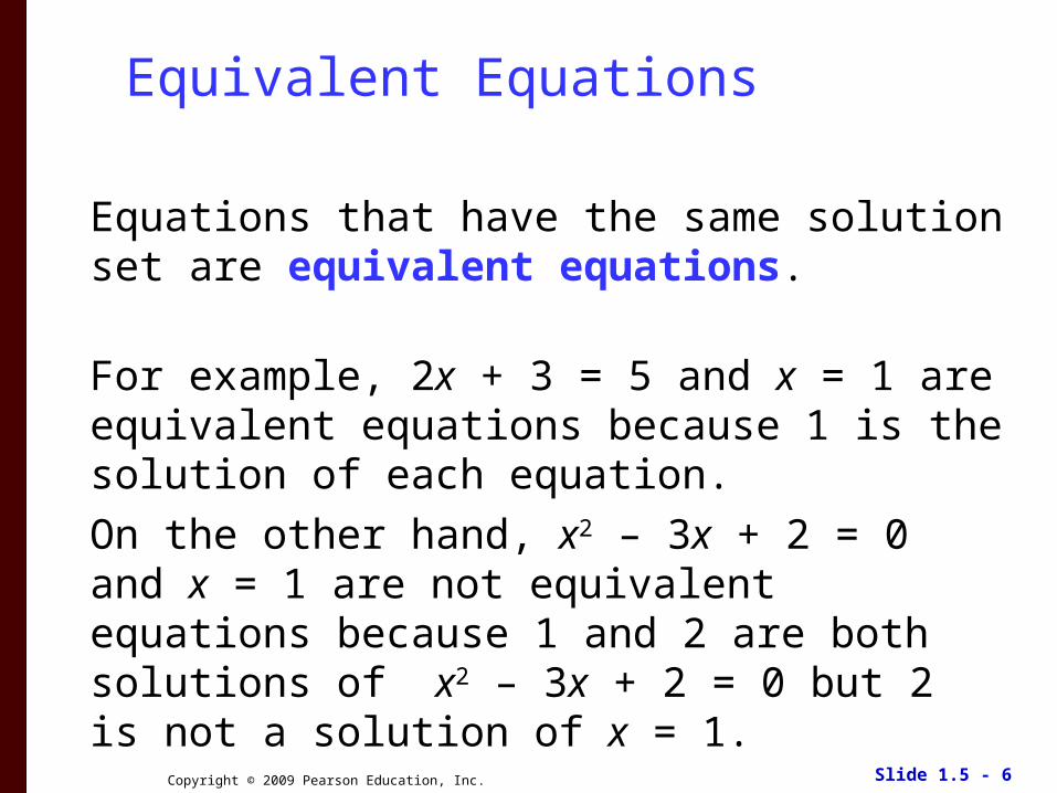
Equivalent Equations

Equations that have the same solution set are equivalent equations.

For example, 2x + 3 = 5 and x = 1 are equivalent equations because 1 is the solution of each equation.

On the other hand, x2 – 3x + 2 = 0 and x = 1 are not equivalent equations because 1 and 2 are both solutions of x2 – 3x + 2 = 0 but 2 is not a solution of x = 1.


Equation-Solving Principles

For any real numbers a, b, and c:

The Addition Principle:

If a = b is true, then a + c = b + c is true.

The Multiplication Principle:

If a = b is true, then ac = bc is true.


Example

Solve:

Solution: Start by multiplying both sides of the equation by the LCD to clear the equation of fractions.

3

4x 1

7

5

203

4x 1

20

7

5

203

4x 201 28

15x 20 28

15x 20 20 28 20

15x 48

15x

15

48

15

x 48

15

x 16

5


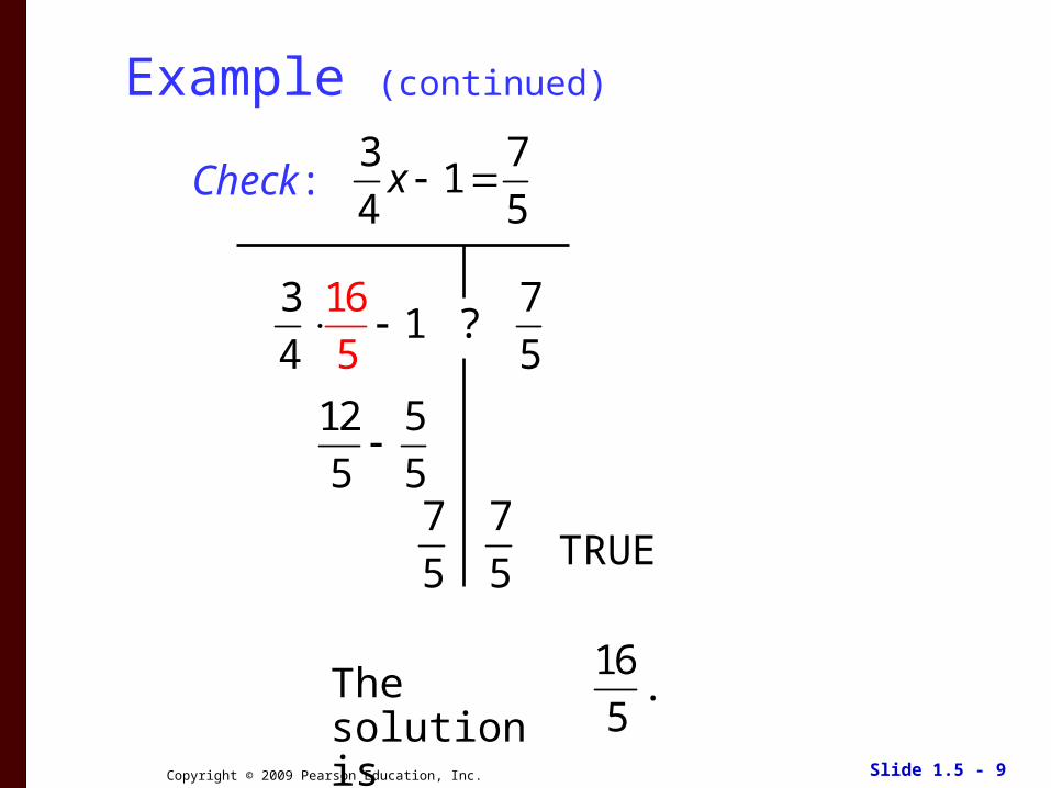
Example (continued)

Check:

3

416

5 1 ?

7

5

12

5

5

57

5

7

5

3

4x 1

7

5

The solution is 16

5.

TRUE


Example - Special Case

Solve:

Solution:

24x 7 17 24x

24x 7 17 24

24x 24x 7 24x 17 24x

7 17

Some equations have no solution.

No matter what number we substitute for x, we get a false sentence.Thus, the equation has no solution.


Example - Special Case

Solve:

Solution:

3 1

3x

1

3x 3

1

3x 3

1

3x

1

3x

1

3x 3

3 3

There are some equations for which any real number is a solution.

Replacing x with any real number gives a true sentence. Thus any real number is a solution. The equation has infinitely many solutions. The solution set is the set of real numbers, {x | x is a real number}, or (–∞, ∞).


Applications Using Linear Models (optional)

Mathematical techniques are used to answer questions arising from real-world situations.

Linear equations and functions model many of these situations.


Five Steps for Problem Solving (optional)

1. Familiarize yourself with the problem situation.

Make a drawing Find further information

Assign variables Organize into a chart or table

Write a list Guess or estimate the answer

2. Translate to mathematical language or symbolism.

3. Carry out some type of mathematical manipulation.

4. Check to see whether your possible solution actually fits the problem situation.

5. State the answer clearly using a complete sentence.


The Motion Formula (optional)

The distance d traveled by an object moving at rate r in time t is given by

d = rt.


Example (optional)

America West Airlines’ fleet includes Boeing 737-200’s,each with a cruising speed of 500 mph, and Bombardier deHavilland Dash 8-200’s, each with a cruising speed of 302 mph (Source: America West Airlines). Suppose that a Dash 8-200 takes off and travels at its cruising speed. One hour later, a 737-200 takes off and follows the same route, traveling at its cruising speed. How long will it take the 737-200 to overtake the Dash 8-200?


Example (continued) (optional)1. Familiarize. Make a drawing showing both the known and unknown information. Let t = the

time, in hours, that the 737-200 travels before it overtakes the Dash 8-200. Therefore, the Dash 8-200 will travel t + 1 hours before being overtaken. The planes will travel the same distance, d.


Example (continued) (optional)

We can organize the information in a table as follows.

2. Translate. Using the formula d = rt , we get two expressions for d:

d = 500t and d = 302(t + 1).Since the distance are the same, the equation is:

500t = 302(t + 1)

Distance Rate Time

737-200 d 500 t

Dash 8-200 d 302 t + 1

d = r • t



500t = 302(t + 1)500t = 302t + 302198t = 302 t ≈ 1.53

4. Check. If the 737-200 travels about 1.53 hours, it travels about 500(1.53) ≈ 765 mi; and the Dash 8-200 travels about 1.53 + 1, or 2.53 hours and travels about 302(2.53) ≈ 764.06 mi, the answer checks. (Remember that we rounded the value of t).

5. State. About 1.53 hours after the 737-200 has taken off, it will overtake the Dash 8-200.

3. Carry out. We solve the equation.


Simple-Interest Formula (optional)

I = Prt

I = the simple interest ($)

P = the principal ($)

r = the interest rate (%)

t = time (years)


Example (optional)

Jared’s two student loans total $12,000. One loan is at 5% simple interest and the other is at 8%. After 1 year, Jared owes $750 in interest. What is the amount of each loan?



Solution: 1. Familiarize. We let x = the amount borrowed at 5%

interest. Then the remainder is $12,000 – x, borrowed at 8% interest.

Amount Borrowed

Interest Rate

Time Amount of Interest

5% loan x 0.05 1 0.05x

8% loan 12,000 – x 0.08 1 0.08(12,000 – x)

Total 12,000 750



2. Translate. The total amount of interest on the two loans is $750. Thus we write the following equation.

0.05x + 0.08(12,000 x) = 750

3. Carry out. We solve the equation.

0.05x + 0.08(12,000 x) = 750

0.05x + 960 0.08x = 750

0.03x + 960 = 750

0.03x = 210

x = 7000

If x = 7000, then 12,000 7000 = 5000.



4. Check. The interest on $7000 at 5% for 1 yr is $7000(0.05)(1), or $350. The interest on $5000 at 8% for 1 yr is $5000(0.08)(1) or $400. Since $350 + $400 = $750, the answer checks.

5. State. Jared borrowed $7000 at 5% interest and $5000 at 8% interest.


Zeros of Linear Functions

An input c of a function f is called a zero of the function, if the output for the function is 0 when the input is c. That is, c is a zero of f if f (c) = 0.

A linear function f (x) = mx + b, with m 0, has exactly one zero.


ExampleFind the zero of f (x) = 5x 9.

Algebraic Solution: 5x 9 = 0 5x = 9 x = 1.8

Using a table in ASK mode we can check the solution. Enter y = 5x – 9 into the equation editor, then enter x = 1.8 into the table and it yields y = 0. That means the zero is 1.8.


Example (continued)

Find the zero of f (x) = 5x 9.

Graphical Solution or Zero Method:

Graph y = 5x – 9.

Use the ZERO feature from the CALC menu.

The x-intercept is 1.8, so the zero of f (x) = 5x – 9 is 1.8.


Formulas

A formula is an equation that can be used to model a situation.

We have used the motion formula, d = r • t.

We have used the simple-interest formula, I = Prt.

We can use the equation-solving principles to solve a formula for a given variable.


Example

Solve P = 2l + 2w for l.

Solution:

P 2l 2w

P 2w 2l

P 2w

2l

l P 2w

2The formula can be used to determine a

rectangle’s length if we know its perimeter and width.

Copyright © 2009 Pearson Education, Inc. CHAPTER 1: Graphs, Functions, and Models 1.1 Introduction...

Documents

Transcript of Copyright © 2009 Pearson Education, Inc. CHAPTER 1: Graphs, Functions, and Models 1.1 Introduction...