Copyright © 1991, by the author(s). All rights reserved ...

Copyright © 1991, by the author(s).

All rights reserved.

Permission to make digital or hard copies of all or part of this work for personal or

classroom use is granted without fee provided that copies are not made or distributed

for profit or commercial advantage and that copies bear this notice and the full citation

on the first page. To copy otherwise, to republish, to post on servers or to redistribute to

lists, requires prior specific permission.

GENERALIZING THE TWIST AND

FLIP PARADIGM

by

Ray Brown and Leon Chua

Memorandum No. UCB/ERL M91/24

17 March 1991

GENERALIZING THE TWIST AND

FLIP PARADIGM

by


Memorandum No. UCB/ERL M91/24

17 March 1991

ELECTRONICS RESEARCH LABORATORY

College of EngineeringUniversity of California, Berkeley

94720

Generalizing the Twist and Flip Paradigm


University of California, BerkeleyDepartment of Electrical Engineering

and Computer Sciences

March 17, 1991

Abstract

Li this paper we generalize the horseshoe twist theorem of [Brown& Chna, 1991] and derive a wide dass of ODEs, with and without dissipation terms, for which the Poincare can be expressed in dosed formas FTFT where T is a generalized twist. We show how to approximatethe Poincare maps of nonlinear ODEs with continuous periodic forcing by Poincare maps which have a dosed form expression of the formFT1T2... T„ where the T,- are twists. We extend the twist and flip tothree dimensions with and without damping. Further, we demonstratehow to use the square-wave analysis to axgue the existence of a twistand flip paradigm for the Poincare map of the van der Pol equationwith square-wave fordng. We apply this analysis to the cavitationbubble oscillator that appears in [Parlitz, et. al., 1991] and prove avariation of the horseshoe twist theorem for the twist and translate

used by Parlitz. We present illustrations of the diversity of the dynamics that can be found in the generalized twist and flip map, andwe use a pair of twist maps to provide a spedflc and very simple illustration of the Smale horseshoe. Finally, we use the twist and translateof [Parlitz, et. al., 1991] to demonstrate that the addition of suifldentlinear damping to a dynamical system having PBS chaos may causethe chaos to become visible.

1 Introduction

In [Brown & Chua, 1991] three conjectures were stated about the presence ofhorseshoes in a very general class of ordinary differential equations (ODEs).For the case when the Poincare map is of the form FTFT where T is thesimple twist [Brown & Chua, 1991], all three of these conjectures have nowbeen proven. The proofs of these conjectures depend on an important intermediate result. The conjectures and this intermediate result will all bestated in Sec. 2, with a brief indication of the proofs which may be foimd indetail in [Brown,1990].

Encouraged by our success in proving the existence of horseshoes for thesimple twist and flip map, it is reasonable to eisk if this result is simply aspecial case, or is it part of a broader theory. We argue that it is indeedpart of a broader theory through the following steps: In Sec. 3 we showthat the class of ODEs having Poincare maps of the form FTFT, where Tis a generalized twist is very large, and we derived a lemma that gives ussome idea of how large this class is. This lemma provides a mechanismfor obtaining the Poincare map in closed form when a square-wave forceis present, and we demonstrate this by deriving five broad classes of non-dissipative, nonlinear, square-wave forced ordinary differential equations andtheir closed form Poincare maps.

In Sec. 4 we go on to show that what we have done for non-dissipativeequations of Sec. 3.2 can also be done for equations having a damping ordissipative force, and thus we are able to obtain a closed form solution forthe Poincare map of a large class of damped ODEs.

In Sec. 5 we outline the proof of a generalization of the horseshoe twisttheorem.

In Sec. 6 we demonstrate how to extend the twist and flip paradigm fromsquare-wave forcing to the case of continuous periodic forcing.

In Sec. 7 we show how the twist and flip can be generalized to threedimensional systems.

In Sec. 8 we extend the concept of the twist map by defining the conceptof a two dimensional shear map.

In Sec. 9 we indicate how to use the square-wave analysis to find a twistand flip map in the van der Pol equation and suggest that the complexity ofthe van der Pol equation is explained by the twist and flip paradigm.

In Sec. 10 we will show that in place of the twist and flip map, some

equations have a twist and translate paradigm. This fact, found in the cav-itation bubble oscillator of [Parhtz, et. al., 1991], suggests an extensionof our results to include Poincare maps of the form LT where L denotes atranslation. In fact we may extend the twist and flip paradigm to includemaps of the form T2T1 where Ti is a twist map, and T2 is any combinationof twist maps, flip maps, translate maps, or diffeomorphism defined by anylinear second order ODE. In this section we prove the horseshoe twist andtranslate theorem for the non-dissipative twist and translate map.

In Sec. 11 we illustrate the diversity of the dynamics of the twist and flipmap by presenting four figures consisting of unstable manifolds and ellipticregions generated by generalized twist and flip maps. In this section we alsoillustrate the Smale horseshoe using a map of the form FT2T1, where Tj axeboth simple twist maps. The computer code for this illustration is included.

In Sec. 12, we illustrate a basic mechanisn of the onset of chaos in abroad class of dynamical systems using the damped twist and translate mapof Parlitz. In particular we show that in the case of linear damping, thecomplexity of,a dynamical system can be fotmd in the non-dissipative formof the equations describing the system and that this complejdty may becomevisible with the addition of sufficient damping even though linear dampingcannot create horseshoes.

2 Proof of Conjectures for the HorseshoeTwist Theorem

We have stated the horseshoe twist theorem for the Poincare map of the firstorder non-linear, square-wave forced system of ODEs in [Brown & Chua,1991]. We restate this ODE here for convenience of reference:

X= ( X- asgn(sin(a;<))) ^ (1)

y={ X—asgn(sin(wt))) x—a sgn(sin(a;t))) ^where a > 0. In the following discussion we will adopt the same terminologyused in [Brown & Chua, 1991].

Let M be the unstable manifold of FT at a hyperbolic fixed point, whereM consists of two branches that are joined at the fixed point. It was proven

in [Brown h Chua, 1991] that the local unstable manifold of one of thesebranches lies on the right side of the vertical axis. Recall that we labeledthis branch as Mrhs.

Our starting point is the horseshoe twist theorem of [Brown Chua,1991], hereafter referred to as the horseshoe twist theorem I. The key to theproof of the generalized horseshoe twist theorem, hereafter referred to as thehorseshoe twist theoremII, can be found in the following theorem,^ theorem 2,which states that the right hand branch, M,iu, of every homoclinic manifold(i.e., M=S, where S is the stable manifold) from a fixed point of FT lyingon the positive vertical axis lies in an annulus bounded away &om the fixedpoints of T. From this we conclude that if M contains a fixed point of T itcannot be homoclinic.

Before indicating the proof of these results we recall some definitions from[Brown & Chua, 1991].

We have defined Cr to be the circle of radius r centered at (a,0) anddefine to be the circle of radius r centered at (—a, 0).

Using these definitions we define Gr to be the intersection of Dr andthe right half plane {{x,y)\x > 0} and let Hr denote the intersection ofand the left half plane. We will use Sihs to denote the branch of the stablemanifold that originates on the LHS of the plane. This must exist by lemma7 of [Brown & Chua, 1991]

Lemma 1 if M = S then Mrfis = Sihs-

Proof: Suppose that M=S and let be the circle centered at (—a, 0) havingradius r.

Assume that the right hand branch of the stable and unstable manifoldsmeet, and thus coincide. By lemma 7 of [Brown & Chua,1991] Mrhs begins inthe interior of Dr . By the same lemma Srhs lies on the RHS of the verticalaxis and lies outside of Dr. To meet Srhs on the RHS of the vertical axis,

Mrhs must cross this circle by continuity. But this cannot happen unless Mrhsh£is already intersected the vertical axis.

But if Mihs intersects the vertical axis, so does S and at the same point,since by lemma 5 [Brown & Chua, 1991], R(M)=S, where R denotes refiec-

complete pioof of the horseshoe twist theorem II can be found in a recent Ph.D.dissertation [Brown, 1990].

tion about the vertical axis. So if S=M, R(Mrhs) meets Suu, and so mustcoincide. I

We recall without proof the following proposition [Brown & Chua, 1991]

Proposition 1 Let (0,y) he a hyperbolic fixed point of FT on the positivevertical axis. Let M be the unstable manifold at (0,y). Then there is a pointwhere M crosses the vertical axis other than the fixed point (0,2/).

Before we state and prove theorem 1 we need the following 2 lemmas.

Lemma 2 Let {Q,y), y > 0 be a hyperbolic fixed point for FT and let Mrhsbe as in lemma 1. Let p be the point on the vertical axis that is in M, and hasshortest arc length measured along the unstable manifold to the point (0,y).Let Za be (FT)"^(p). Let r = y/y^ + a^, and let = \\Za —a||. Define theannulus Aa by the equation

Aa = {z|ra < ||z - a|| < r}

Let V = (M,h3 n A„) Then T(V - {p}) C H,..

Proof: We have the following facts: T(V) C Cr, T(0,j/) = (0, —2/)» andT(za) = —p. By the choice of z®, there can be no other points of T(V) onthe vertical axis.other than (0,—y) and —p, so that T(V) must He entirelyinH,..!

Weneed the following lemma from [Brown, 1990] in the proof of theorem 1

Lemma 3 Given a hyperbolicfixed point of FT, let S be the stable manifold,and M the unstable manifold at this fixed point. IfS = M., then

PT(M) = M

where P is reflection about the horizontal axis.

Proof: FT(M)=RPT(M)=M=R(M). Therefore RPT(M)=R(M), so thatPT(M)=M. I

Theorem 1 (Homoclinic Manifold Theorem) IfM is a homoclinic manifold of FT, then M^hs 1^^^ annulus bounded away from the fixed pointsofT.

Proof: Since M is homoclinic we have M = S = R(M). Let Mrfu, be thebranch of M Ijring in the RHS of the plane. R(Mriu,) = Sihs (where "Ihs"stands for left hand side) and so

R(Mrhs USlhs) = (Mrhs u Sjhs)

forms a connected curve in R^. We will label this curve as N and note that

it contains the branch of the unstable manifold M lying in the RHS of thevertical axis.

Let q be the point other than (0, y) where N meets and crosses the verticalaxisand let = (FT)~^(p). By lemma 7 [Brown & Chua,1991] and lemma3above, PT(N) = N.

For any annulus A, we have PT(A) = A. So, PT(A fl M) = A fl M andalso, PT(A n N) = A n N. This relation must hold for Aa- By the choiceof Za we have T(Aa HMrhs) must lie entirely on the LHS of the vertical axis(lemma 2 above), except for the point q which must lie on the vertical axis.For convenience we define = (A® H Mhu,). Therefore PT(Ma) = Sihs-Since Srhs lies entirely in Aa, we conclude that N is contained entirely inA«UR(A„).

Now To ^ ra. If w is a fixedpoint of T that is in Mrhs? then FT(w) = F(w)which is on the LHS of the vertical axis, i.e., ro < r^, hence cannotintersect 0^ and so N cannot intersect Cro UDro*

We conclude that M is bounded away from the circle of fixed points ofT; namely, Cro- Thus N lies inside the circle C, and outside the circle C,where s > tq. 1

Corollary 1 Assume the definitions of the above lemma. ^ a homo-clinic manifold, it must meet and cross the negative vertical axis.

Proof: Follows directly from lemma 2 above. I

Corollary 2 Assume the definitions of the above lemma. If Mrhs crossesthe positive vertical axis at a point other than a fixed point, then it is ac-manifold.

Proof: Follows directly from corollary 1 above. I

Theorem 2 (Horseshoe Twist Theorem 11) Let (0,y), y > 0, 6e a hyperbolic fixed point of FT and let M he the unstable manifold of FT at thishyperbolic fixed point. If Mrhs contains a fixed point of T, then FT ha^ ahorseshoe, and hence the Poincare map FTFT also has a horseshoe.

Proof: By theorem 1 if Mrhs contains a fixed point of T then it cannotbe homodinic. Mrfa must meet the vertical axis by proposition 1, at p amdby lemma 5 [Brown & Chua, 1991] this is a homodinic point. If M meetsthe stable manifold at this point there is a horseshoe by [Smale, 1965]. Weassert that M cannot be tangent to the stable manifold at this point. Thusthere exists a horseshoe. I

We may now restate conjecture 3 of [Brown & Chua, 1991] as a corollary.

Corollary 3 Given a hyperbolic fixed point (0, y), with r = y/y^ -{• andTo = 2a;[r/2a;], a sufficient condition for the unstable manifold M of thisfixed point to be a c-manifold is that the two circles,

(x - af + = To

and

(x + a)^ + y^ =

intersect.

Proof: Recall that by the definitions in [Brown & Chua, 1991] the firstcircle above is denoted and the second is denoted D^. Assume these twocircles intersect. Note that the drcle Cro is a circle of fixed points of T.

If Mrhs crosses the positive vertical axis at a point other than the fixedpoint we are done by corollary 2. Thus assume that Mrhs crosses the negativevertical axis. By lemma 2 and the fact that Mrhs crosses the negative verticalaxis, this crossing must lie below the circle of fixed points of T. Hence thereare points in Mrhs that lie above the drcle 0^ and below C^o and so becauseDr intersects Cro ^rhs is connected, it must intersect Cro thuscontain a fixed point of T. By theorem 2, M must be a c-manifold. I

Remark 1: We recall that another form of this condition is given by thefollowing inequality:

r < 2a-{-ro

or

r mod (2a;) < 2a.

Remark 2: The horseshoe twist theorem I of [Brown & Chua, 1991] isnow a special case of corollary 3. In particular the horseshoe twist theorem of[Brown & Chua, 1991] required that two conditions be satisfied. The secondcondition of the two, namely, Tq > (c —a)^, is equivalent to the condition ofcorollary 3. Therefore, corollary 3 is more general than the horseshoe twisttheorem I and, by inspection, can be seen to be much easier to verify.

3 Differential Equations Having Closed FormPoincare Maps

Our success in deriving a formula relating the parameters of an ODE to chaosdepended on the existence of a closed form expression for the Poincare map.This suggests the following question: How common are nonlinear, periodically forced ODEs having closed form Poincare maps? To aid in answeringthis question we have the following factorization lemma.

3.1 Factorization Lemma for the Poincare Map ofCertain ODEs

Lemma 4 Let x(t) be a solution of

X= G(x, t), and x(0) = Xq (2)

where (xo,f) € R" x R. Also, suppose that there exists a constant p suchthat for all (x, t) G R" X R the function G satisfies the relation

- G(x, t -1- p/2) = G(-x, t) (3)

Let

y(<) = -x(( + p/2)

for 0 < f < CO. Then y(f) is a solution of the equation

y = G(y,t), and y(0) = -x(p/2).

Proof: Let u{t) = —x(f + p/2). Then u(0) = —x(p/2) and

u = -k{t + p/2) =

-G(x(^ + p/2), <+ p/2) = G(-x(t + p/2), t) =

G(u,<)

Therefore, u(i) = y{t) = —x(t +p/2). IRemark We note that G in Eq.{ 2) is periodic as a function of t with

period p. If we let Tf be the one parameter family of phase plane diffeomor-phisms in defined by Eq.( 2), then the Poincare map is Tp. We use thisfact in the following corollary.

Corollary 4 Let F be a 180 degree rotation about the origin in R^ andlet Tt be the one parameter family of phase plane diffeomorphisms definedby Eq.( 2). Then the Poincare map for Eq.( 2), i.e. Tp, is given by thediffeomorphism, $ o/R^ defined by

$(xo) = FTp/2FTp/2(xo)

Proof: Let x(t,Xo) be the solution of Eq.( 2) over the interval [0,p/2] with

x(0,Xo) = Xo, and let y(<,yo) he the solution of Eq.( 2), for 0 < t < p/2,having the initial condition

yo =Xi = -x(p/2,Xo)

Then, by lemma 4, for 0 < t < p/2 we have

x(t+p/2,Xo) = -y(^,xi)

K we take t = p/2 in corollciry 4 we have the relation

x(p,Xo) = -y(p/2,xi)

where

Xi = -x(p/2,Xo)

We conclude that

x(p,Xo) = FTp/2FTp/2(xo)•

Remark: This corollary is also true for R".Since we will always assume p = 21^1uj we will henceforth drop the sub

scripts and write the Poincare map simply as FTFT.

3.2 Some Differential Equations for Which there areClosed Form Poincare Maps

With the above factorization lemma in hand we now determine several classes

of ODEs for which the Poincare map can be obtained in closed form.It may be readily verified that the equations of this section satisfy the

hypothesis of lemma 4, where p = 2t/uj, and therefore by corollary 4 thePoincare map is of the form FTFT.

We have the following convenient definition used extensively in the following sections:

Definition sg(t) = sgn(sin(<)).

Class 1 is determined by the pair of equations:

X = -yfWy = (x-asg{(jjt))f{X)

where A= ^(a; —asg(a;<))2 -}- y^.For f(u) = u this equation is the same as in [Brown & Chua, 1991].The Poincare map is FTFT where T is the solution of the equations

^ = -yfWy = (x-a)/(A)

a.t t = tt/w, where A= y(a; —a)^ y^, and F is the 180 degree rotation.Note that A is a constant defined by the initial conditions and represents

a constraint on the variables x and y. Also note that since

J =-(x-a)/3,10

in the last pair of equations above, the phase portrait of the solutions consistsof a continuum of circles centered at (a,0). In particular, {x{t),y(t)) mustlie on a circle of radius A centered at (ffl,0).

The matrix form of the twist map for class 1 is given by

( a:(f) \ / cos (/(A)f) —sin ( /(A)t) X/xo — /a^

V )/ \ sin (f(X)t) cos ( ) \ Vo ) \ 0>Class 2 is determined by the following equations:

® ~ asg(wt))2 + (1 - P)y2 (4)

y = {x- - asg(wt))2 + (1 - h'̂ )y^ )H(x,y) (5)Where k is the elliptic modulus and

_ ^(x - a3g(fa;<))^ + (1 -y/(x-asg{wt)Y + y^

where /(r) is any function of r.

The Poincare map is given by FTFT where T is the solution of the equation

^ = -yf{y/{x - ay -h (1 - A;2)y2 "jhix, y) (6)y= {x- a)f{y/{x - af + (1 - fc2)y2 ^h{x, y) (7)

where,^ ^(x- af + (1 -

h[x,y) = ^ / .- a)2 + y2

evaluated at the time t = tt/w, and, cis above, F is a 180 degree rotationabout the origin. Note that as for class 1 equations the phase portrait ofEqs. 6 and 7 is also a continuum of circles centered at (a, 0) since,

11

We may write out the solution of the latter autonomous vector ODEsexplicitly using the addition formulae for the Jacobi elliptic functions:

__ (xq - a)cn(/(r)t, k) - Kyosn(f{r)t, fe)dn(/(r)t, k)CD?{f{r)t, fe) + K'̂ siL^(f(r)t, k)

, _ K(xo - a)sn(/(r)f, k) + yocn(/(r)t, fc)dn(/(r)t, k)^ aa?{f(r)t, k) +K^sn^ k)

where a;(0) = Xq, y(0) = yo, r = \](xq - a)^-{• yl, K = ^1 - {kyolrf,and sn, cn, and dn are the Jacobi elliptic functions having elliptic modulusk. From this point on we will drop reference to the elliptic modulus k in theelliptic functions unless it is needed for clarification.

The matrix form of the twist map for class 2 is given by:

( x{t) ^

KfW j

where

c(t) = l/[ cn^(/(r)t) + A''sn^(/(r)«)]For k = 0 class 2 reduces to class 1.

Class 3 equations are obtained from class 2 equations by letting k = g{X)in Eq. 4 and 5, where ^(A) is any function. Since A= yf(x —a)^ + y^ isdetermined by the initial conditions we see that the elliptic modulus is alsodetermined by the initial conditions. In this case, the matrix form of thetwist map is the same as in class 2, except that k = ^(A).

Class 4 equations are those motivated by the function

x{t) = Acn(At + fc) + a

/ ca{f{r)t) -Ksa{f{r)t) dn(/(r)t) \ / xo-a

VKsa{f(r)t) cn(/(r)t) dn(/(r)t) / \ yo

where A^ = 0.5[ (1—2fc^)(a:o—— 2k^)^(xQ —aY + 4(i;§ + k^{xo —a^) ]This function solves the ODE

X+ p(x,y)(l —2k^)(x —a) + 2k^(x —a)^ = 0

12

where, p(a;, y) = 0.5[ (1—2fc^)(a;—a)^+^(l —2k'̂ y(x — + 4(x^ + k^(x —a)^) ]It should be noted here that the appearance of a term containing i, such

as occurs above, does not necessarily imply the presence of damping in theODE.^ On the contrary, the solution of this equation consists of concentricclosed curves parameterized by Adefined above. If we replace a in the aboveequations by a sg(a;t) we obtain an ODE having a square-wave forcing termwhose Poincare map, is FTFT, where

T(r, y) = { Acn(At + ^) + a,—A^sn(At -f- ^)dn(At -H ^))

and where t = tt/o;.When = 0.5, the equation for T reduces to a variation of Duflfing's

equation, namely,r -1- (x —a)^ = 0

In this case A^/4 = 4xo + (xo —a)^. If we replace a by asg(a;t) we get asquare-wave forced variation of Duifing's equation:

X"f (x — = 0

The Poincare map of this equation is given by FTFT where the twocomponents of T are

x(t) = Acn(At -I- ) + ax(t) = —A^sn(At -I- 0, "v/OlK )dn(A< + 0, )

Also note that by taking A; = 0 we obtain a special case where T isexpressible in terms of sines and cosines:

a;(t) = Acos (At + 0) ax(t) = —A^ sin (At -t-

These two functions define a family of ellipses centered at (a, 0). If theseequations are expanded using the addition formula for sine and cosine andwe note that xo = Acos(^) + a and xq = —A^ sin(^) then

^To see this in a simpler case consider the equation

X+ x/{x^ -H 1)= 0

which is solvable in terms of elhptic functions.

13

= 0.5[ (a;o - a)^ + ^(xo - +4ig ]

and we have the following matrix form for the twist T:

^ cos(At) —sin(A<)/A

^ Asin(At) cos(A<)

^ Xq Qt

\ yo

In this case, the ODE associated with T is given by:

+

X+ 0.5[ (x —aY + y(x —— a). = 0

In this map, the twisting takes place around an ellipse rather than a circle.When fc ^ 0 in class 4, it is possible to carry this generalization one step

further by cissuming that k = flr(A), where as before g{X) is amy function.In this case the equation for A can be very complex. For example, if = A,then this equation becomes

A^ = 0.5[ (1 —2A)(xo - aY + ^(1 —2A)2(xo —a)^ +4(xg + A(xo —a)^) ] .

Class 5 equations for T are given by general elliptic differential equations.See pavis, 1960], page 209:

y = Ai- By Cy^ + Dy' (8)

This equation when considered as a complex ODE is solved in terms of ellipticfunctions, [Davis,1960]. Unlike the case for linear equations, the real andimaginary parts of the complex solution are not solutions of Eq. 8. To obtainreal solutions in terms of elliptic functions we consider only special cases, forexample:

y = -Ay - By^ (9)

where A > 0 and B > 0. This equation has the following real solution:

y{t) = Cdn(At + k)

where k^ = (2A + A)/A^ and = 2X^/B.

14

As in the above examples, the square-wave forced equation is obtainedby replacing y by (y —asg(a;t)) in the equation for T.

From the form of this solution we see that the initial conditions can

affect the amplitude, frequency, and the elliptic constant, fc, of the solutionsof Eq.( 9).

Remark: The above equations may be divided into two groups. Groupone arises from a first order vector system in R^. Group two arises from asecond order scalar ODE. Thus we see that Classes 1,2,3 are of increasingcomplexity from group 1, whereas classes 4 and 5 are from group two andalso of increasing complexity.

4 Differential Equations with Damping whichhave Closed Form Poincare Maps

Corresponding to the above described five classes of undamped DDEs thereare five classes of damped DDEs having Poincare maps in a closed form.We illustrate how to introduce damping into these equations in a specificexample and a general example only, without deriving the five classes.

4.1 The Damped Twist

To obtain ODEs with damping having a Poincare map in closed form let usbegin with the following example which we will show how to generalize inthe following section. Consider:

a;(t) = Aexp(—at)cn(u) (10)

where u = A(exp(—at) —l) -f Aand 9 are arbitrary constants.Taking the first derivative we get

X= —ax + aA^ exp(—at)sn('u)dn(u) (11)

The ODE for which a;(t) is the solution is given by

X-h 3ai -f lo^x 2a^k^x^ = —a^(l ~ 2k^)nx (12)

where ji = A^exp(—2at). The factor contains both the arbitrary constantof integration. A, and time, t, and thus it appears at first that Eq. 12 is not

15

autonomous. However, by using identities for the Jacobi elliptic functionsthe factor n may be eliminated. In particular we may do so by solving thequadratic equation:

(1 — + (2A;^ —\)x^n —(Px"* + (x/or + x)^) = 0 (13)

This is a quadratic equation for and so the positive root must be chosen. The origin of this quadratic equation is as follows. From [Bowman,1961]we know that the Jacobi cn satisfies the ODE:

X = —(1 —2P)x —2A:^x^

where fc is a parameter of the ODE which turns out to be the eUiptic modulus.This equation has a first integral

x/2 = -(1 - 2P)a:2/2 - k'̂ x^l2 ^ H/2 (14)

where H is determined by evaluating the functions sn, cn, dn at t = 0.Specifically H = (1 —fc^). By noting from Eq. 10 that

Ax = A^exp(--at)cn(u)

and

(x -|- ax)Ia = A^ exp(—Q;t)sn(u) dn(u)

we obtain Eq. 13 from Eq. 14.The square-wave forced differential equation may be obtained as before

by replacing x by (x —asg(a;t)) in Eq. 12.More complex relationships for (i may be obtained by allowing fc to be a

function of (jl. For example, if fc = /i, then the equation for fi becomes

—2x^fi^ —(1 -- x'*)/i^ -I- x^fi -H (x/of 4- x)^ = 0

Doing this makes the elliptic modulus^ fc, a function of the initial conditionsof the ODE.

4.2 Generalizations

We may generalize the idea presented in the preceding section by the following lemma:

16

Lemma 5 Assume the solutions of the following the differential equationsare unique for each set of initial conditions:

x{t) = G{u){x —asg(a;<)) —H(u)yyfu^ —

y{t) = G{u)y + H{u){x - asg{u}t))yju'̂ - k^y^where

= {x- asg(ijf))^ +

x(0) = Acn(0) and y(0) = Asn(^), and G^ H are continuous.Define two functions g and f by the differential equations

g\t, A) = g{t, \)G{g(t, A)) and g(0, A) = A

f(t, A) = g{t, X)H{g(t, A)) and /(O, A) = 0and then define

x{'kI(jj) = y(7r/a;, A)cn(/(7r/tj, A) + ^) + a

y(7r/a;) = y(7r/a;, A)sn(/(7r/cj, A) + 9)If the map T is defined by the equation

T(®o,yo) = {x(ir/w),y{irlu))

then the Poincare map of the square-wave forced system above is FTFT.

Proof: Apply the factorization lemma to exchange the square-wave forcedsystem for an autonomous equation which determines T. Differentiate thefunctions to obtain the autonomous ODEs and use the relation g^ =(x —a)^ -f-y^ to eliminate the arbitrary constants from these equations. Thenby the uniqueness assumption we are done. I

For the case where A: = 0, the matrix form of the twist map given by thislemma is:

( \ / cos(/(t)) -sin(/(t)) \ f Xq-a \ / a^I = c(t, A) I I -f-

Vy(0 / \ sin(/(<)) cos(/(t)) J \ yo J \0 )

where c(t,A) = y(t, A)/A, y(0,A) = A, and/(0,A) = 0, A^ = (a;o-a)^+yo.

17

Remark: Because we have above a pair of first order equations theremust be two arbitrary constants in the solutions. These constants are A and0. Note, however, that 9 makes no contribution to the twisting action.

Remark: It would appear that if we add damping to a twist map thatappears in a twist and flip map the combined damped twist and flip wouldconverge to a fixed point since the effect of damping is to decrease the distancebetween any point and the center of the twist. However, lemma 13 of [Brownh Chua, 1991] implies that if the damped twist maps a point to the righthand side of the vertical axis near the center of the twist (a, 0), then the flipmust map it to the left hand side of the vertical axis, away from the centerof the twist. At best, the damped twist and flip map can settle down to aperiod-two point.

4.3 Generalizations of the Twist Map and the DampedTwist Map

The preceding considerations lead us to a generalization of a twist map anda damped twist map beyond that found in [Brown & Chua, 1991].

Definition: The following functions define a one parameter family ofgeneralized damped twist maps in R^, with parameter t:

x{t) = g{t, A)cn(/(<, A) -b 0) 4- a

j((t) =^(<,A)sn(/(<,A) + «)where Aand $ are determined by a;(0), and y(0), and

and

In the event thatdg .

we have a generalized undamped twist map and the differential equations willnot have a damping factor.

18

Remark: These equations define a twist map because both / and g depend on Awhich is determined by the initial conditions. This generalizationis consistent with our original definition in [Brown & Chua, 1991].

5 Horseshoe Twist Theorem III for Cleiss 1

ODEs

We have the following extension of the horseshoe twist theorem for the equations of class 1:

Theorem 3 Let (0,y), y > 0, 6e a hyperbolic fixed point of FT where T is ageneralized twist having rotation /(r). Assume that f'{y/a^ + ) > 0- Let Mhe the unstable manifold of FT at this hyperbolic fixed point. IfM,hs containsa fixed point ofT, or t/Mrhs contains a point of the circle ||z —a|| = a, thenM is a c-manifold and therefore FT has a horseshoe.

Outline of Proof: It is sufficient to showthat the key lemmas of [Brown, 1990]carry over under these assumptions. In the fixed point lemmas simply replacer by /(r). We assume that / is such that there are hjrperbolic fixed points.Note that all symmetry lemmas are independent of /. The generalized twistis area preserving and the trace of D(FT) is given by:

tr =2(l +^^l^^)-4(a/rrur

The lemma for the slope of the expanding eigenvector is unchanged by /.Further the "energy" lenunas are unchanged by /. Given these facts, thetheorem follows. I

We have the following corollary.

Corollary 5 Given a hyperbolic fixed point (0,y), with r = y/y^ -f a^ andTo < r such that /(ro) = 2ujn, a sufficient condition for the unstable manifoldM of this fixed point to be a c-manifold is that the two circles,

(x - af + = rj

and

(x -t- af -I- y^ =

19

intersect, or the two circles,

{x —a)^ + = a^

and

(x + af +

intersect

A simpler form of this condition is

r —To < 2a

When /(r) = r this reduces to

r mod (2a;) < 2a.

We have the following conjecture:Recall that the square-wave forced Duffing equation

X-{• x^ = a sg(a;f)

has the Poincare map FTFT, where T is defined by the map T(a;o,io) ={x{Tr/(jj),x{T/u)) where a;(f) is the solution of

X -jr = a

having initial conditions (xo,xo)-

Conjecture 1 Given a hyperbolic fixed point of FT on the negative verticalaxis, FT has a horseshoe if the unstable manifold associated to this fixed pointcontains a fixed point ofT.

Almost surely a similar theorem is true for classes 2 through 5, but atthis time it has not been proven.

It should be noted that by structural stability of the horseshoe, if a horseshoe twist theorem is proven for classes 1-5, it will also be true for the dampedequations corresponding to classes 1-5 for some sufficiently small dampingfactor.

20

6 Extending the Square-wave Analysis

6.1 Generalizing Square-wave Forcing

The squaxe-wave forcing term is an example of a piecewise constant, periodicfunction. Another example is as follows:

f(t) = ai forO < i < 7r/2

f{t) = a2 for7r/2 <t<ir

f(t) = —02 forir < << 37r/2

f(t) = —oi for37r/2 <t<2Tr

where / is extended to all real t to have period 27r. If this piecewise constant,periodic function is used in place of the square-wave as a forcing term in theequations of the previous sections, we obtain Poincare maps of the formFT1T2FT1T2, where the T,- come from the same equations as T. The onlydifference is that t is now evaluated at 7r/2u;. Thus the T,- are given by

^x('kI2u) \ / cos (/(A)7r/2u;) —sin Xq —ai \

^y(7r/2a;) / \ sin(/(A)7r/2a;) cos (/(A)7r/2w) / \ yo >+

Note that the center of the rotation of Ti is a,*.The above observations lead to a generalization that is suggested in

[Brown & Chua, 1991]. The forcing function of the equations of classes 1through 5 may be any periodic function which is piecewise constant, and thePoincare map is still obtained in closed form. As mentioned in [Brown &Chua, 1991] we may approximate the sine function uniformly by a piecewiseconstant function and thus obtain an approximation of the Poincare mapfor sinusoidal forcing by a Poincare map of the form FTFT where T is acomposition of twists around centers a,-, determined by the sine function. Inthis regard we have the following lemma suggested by Prof. Morris Hirschat U. C. Berkeley.

Lemma 6 Let

x = F{x,g(t))

21

( ai

\ 0

and

y = F(y,fe(«))

for 0 < i < r, where x and y are vectors in R", g,h are real valued (notnecessarily continuous) functions oft, and F is any function inThen for any compact region o/R", we can find a number S small enoughsuch that if

f 1/1(5)^Jo

for 0 <t <T, then (1)||x(<) - !/(<)|| < e

for allO <t <T.Further, (2) the derivatives of x,y with respect to their initial conditions

also satisfies this relationship.

Proof: Since F is we may find a compact neighborhood of N, call it Dr,such that if the solution of the first ODE starts in N it remains in D,. forall 0 < t < r. Likewise for the second equation we can find a compactneighborhood of N, call it Dn such that the solution of the second equationremains in Dn for 0 < i < r. We find a Lipschitz constant, K, for F on theunion of these two neighborhoods and apply theorem 3.3.1 of [Hille, 1969],using the integral assumption to obtain the estimate

||a;(i) - y(<)|| < 8K exp{Kt)

For K fixed, we may choose 6 such that 6K exp(isrr) < e.To prove (2) we invoke Peano's theorem, theorem 3.1 from [Hartman,

1964] and repeat the argument. IThis lemma states that the Poincare map of a periodically forced ODE

from any of the above described classes of DDEs may be approximated uniformly on any compact subset of R^ by a map of the form FTFT, where T isa finite composition of twist maps T,-, each of which can be obtained in closedform. The conclusion we reach is that on any compact set, the Poincare mapof a periodically forced ODE from any of the above described classes can beuniformly approximated on compact subsets by a closed form Poincare map.

We have the following theorem:

22

Theorem 4 (Twist and Flip Approximation Theorem 1) Given theconditions of lemma 6 abovej if the approximating Poincare map has a horseshoe, then so does the periodically forced Poincare map.

Proof: If the approximating Poincare map has a horseshoe, it exists on acompact set by [Smale, 1965]. Since the approximating Poincare map isclose to the periodically forced Poincare map, the horseshoe is preserved bystructural stability. I

Remark: By the same argument we have the following result given theconditions of lemma 6 above. Let the first system be a square-wave forcedsystem and the second system be a approximation of the square-waveobtained by "rounding-off" the comers of the square-wave forcing fimction. Ifthe square-wave Poincare map has a horseshoe, then there exists a "rounded-off" C®® forced Poincare map having a horseshoe also.

Remark Numerical experiments indicate that the above generalizationsallow us to integrate many square-wave forced ODEs by the use of a composition of twist maps followed by a flip. Doing this results in an integrationtechnique using about six lines of code that is about ten times faster thanconventional methods. The following is a computer program in QuickBASICfor the integration of the following class 1 ODE with a sine forcing term:

X = -r{t)y

y = r(t){x —a sin(a;f))

where r(t) = —a sin(u;<))^ + y^.

FOR i=l TO 1000

FORj=l TO Maa = osin(j7r/M)

r = —laY -{-

u = (x —aa) cos(r/M) —ysin(r/M) -1- aa

u = (r —aa) sin(r/M) -j- y cos(r/M)

X = u

y = v

23

PSET (x,y),13NEXT j

FORj=lTOM

aa = —asin(j7r/M)

r = y(x —aaY +

u = (x —aa) cos(r/M) —y sin(r/M) + aa

V= (x —aa) sin(r/M) + y cos(r/M)

X = w

y = v

PSET (x,y),10NEXT jNEXT i

END

RemarkiThe symbol aa in the above code denotes a programming variable.

7 Extensions to Three Dimensions

The Duflfing equation,

X+ ax x^ = a cos(u;<)

can be viewed as an autonomous equation of degree 2 in three dimensions.This three dimensional system is iiot the usual autonomous system obtainedby considering time as a new variable but rather is the following:

X = y

y = z

((i -\-az + 3x^y)/(jj)^ = a^ - (zay + x^)^

For x = y = i = Owe have x = y = 0,2r = 0. This equation is relatedto Buffing's equation by the correct choice of initial conditions. If the originalDuffing equation has the initial conditions x(0) = Xo,y(0) = yo then the

24

third order equation must have the additional condition ^(0) = a —ayo —Therefore, the Poincare map has a natural extension to these equations asthe map associated with the period of an implicit forcing term that is notimmediately visible in the three dimensional ODE.

This extension suggests that we should seek to expand our investigationsto three dimensions. In particular, we seek an extension of the twist and flipmap to three dimensions in such a way that FTFT is a three dimensionalPoincare map for a square-wave forced, nonlinear, first order system of DDEs.We find that this can be done easily, and the three dimensional system isconsiderably larger than the class 1, two dimensional system described earlier.

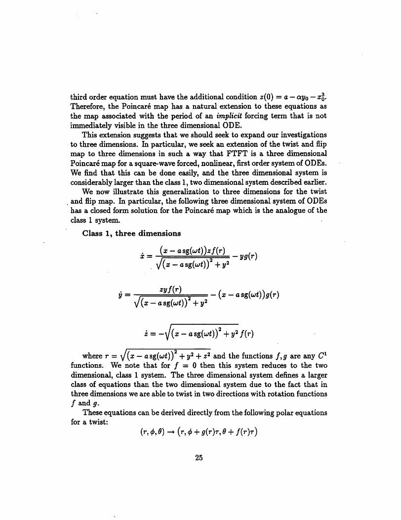
We now illustrate this generalization to three dimensions for the twistand flip map. In particular, the following three dimensional system of ODEshas a closed form solution for the Poincare map which is the analogue of thecla^s 1 system.

Class 1, three dimensions

yj[x-asg{ujt)) +y2

y = _ (j, _ asg(a;i))s(r)V(x-asg(a;t)) -\-y^

z=-yj(r - asg(a;i))^ -1- f(r)

where r = y(x —asg(a;t))^ +1/^ + and the functions f^g are anyfunctions. We note that for / = 0 then this system reduces to the twodimensional, class 1 system. The three dimensional system defines a largerclass of equations than the two dimensional system due to the fact that inthree dimensions we are able to twist in two directions with rotation functions

/ and g.These equations can be derived directly from the following polar equations

for a twist:

(r, <j>, 0) (r, -H g(r)T, 0-f /(r)r)

25

and the polar equations for the associated three dimensional ODE:

(f,^,9) = {0,g{r)J{r))

The rectangular-coordinate matrix form of the twist map in three dimensions about the point (a, 6,c) is given by the following equations: Given apoint in three space, (a;, y,z), define = (x —a)^ {y —a)^ (z —c)^ and

—(z —c)^, then T(a;, y, z) = (u -1- a, u -|- 6, u; -f- c)where,

and.

= C{r,T)cos (y(A)T) —sin (y(A)T) \ / x —a

sin(y(A)r) cos(y(A)r) / \ y-b

C(r, r) = [cos (/(r)r) + (^ - c) sin (/(rjr/s)]

w= cos (/(r)r)(z —c) —ssin (/(r)T)Of course we may introduce damping as we did in the two dimensional

case and obtain three dimensional damped ODEs with square-wave forcing.Class 2, three dimensionsThe three dimensional system of first order, nonlinear ODEs

X = —yz

y = xz

z = —k^xy

where,a:(0) = Acn(^), y(0) = Asn(^), z(0) = Adn(0)

has the Jacobi elliptic functions as a two parameter set of solutions:

x(t) = Xcri{Xt 9^k)y(t) = Asn(At -H 9, k)z{t) = Adn(At -I- 9, k)

By the form of the above solutions, we see that these equations define atwist.

26

The following set of equations have, as a two parameter set of solutions,a twist about the point (a, 0,0)

X = -yz

y = {x- a)zz = —k^(x —a)y

By replacing the constant a by a sg{ujt) we produce a square-wave forcedequation whose Poincare map is of the form FTFT, where T is a twist mapand F is the flip in three dimensions, and T is defined by the Jacobi elliptic functions. By combining the solution of the above equations with a 180degree rotation we obtain a twist and flip map in three space in which thetwisting takes place on a set of concentric elliptic surfaces. The map FTFTdetermined by the twist and flip map is a Poincare map for a three dimensional system with square-wave forcing. The matrix form of this map maybe obtained by using the addition formulae for the Jacobi elliptic functionsand identifying the terms Acn(0), Asn(d), Adn(^) with the initial conditions.

Another generalization is suggested by the following set of functions:

x(t) = XcD.{f{X)g{X)t -}- k)y{t) = XsTL{f{X)h{X)t + $,k)z{t) = Adn(^(A)A(A)t + k)

The above equations define a general three dimensional twist which solvethe following system of equations, where A^ =

X = -yzf{X)g(X)IXif = xzf(X)h{X)IXz = —k'̂ xyg(X)h(X)IX

We may add square-wave forcing as before and generate nonlinear, square-wave forced ODEs in three dimensions whose Poincare maps are of the formFTFT, and where T has a closed form expression of a generalized twist.

This analysis can be extended to obtain further examples of twist onsurfaces. In particular, given any family of concentric, closed surfaces inthree spaces we may obtain a generalization of the twist and flip map. Sucha surface can be defined by a first order partial differential equation (PDE)in three variables, [Sneddon, 1957]. Such a surface is made Up of the integralcurves of a system of three first order ODEs derived from the defining PDE.

27

8 Genersdizing the Twist: She£iring

In this section we will describe a generalization of the twist map when considered in isolation from its role as a Poincare map. Thus we now considerthe twist map as a transformation on and ask how it may be generalized.The following example will provide the motivation for this generalization.

The function x{t) = At2tn(Af -h 9) solves the nonlinear ODE

X — 2xx = 0

where x(0) = lo = Atan(0) and i(0) = xo = A^sec^(^).Similaxly, the function a;(f) = Aaexp(Af) where a = xq/xq and X= xq/xq

solves the ODE

X — = 0

where x(0) = xq, x(0) = Xq.In these examples, the initial conditions affect both the "amplitude" and

"frequency" of the solution as in the case of the twist, except in this casethere is no "bending" action taking place etround closed curves because thesolution of this ODE is not a set of closed curves.

The presence of a stretching action without the bending action of a twistindicates that the above examples are more general than the twist map. Inrecognition of this fact we will define sudi maps as two dimensional shears.

Another example of a shear that is not associated with an ODE is givenby the formula:

T(x,y) = (Ax,2//A)

where, A = (xy)^ -j- 1. This map is modeled after the linear hyperbolicmap (x,y) —> (Ax,y/A), where A is any real number greater than 1, and isdetermined by a partial differential equation.

The primary reason for defining the shear is that it can be used to demonstrate indirectly that the Poincare map of some nonlinear ODEs have a twistand flip action. In the following two sections, we proceed to follow this program and we note that, at present, our methods are somewhat closer to artthan science.

28

9 The van der Pol Equation

In this section we indicate that we can find a twist and flip paradigm in thevan der Pol equation with square-wave forcing; namely:

f —€(1 —x^)x -I- Aa; = a sg(w<)

Since it is not possible to drop the damping term in this equation at this pointwithout losing aUof the interesting dynamics, let us retain it for now. We firstnote that the vector form of this equation in does satisfy the conditions ofthe factorization lemma, hence the Poincare map can be factored as FTFT.We now determine the nature of T from the following autonomous equation:

X—e(l —x'̂ )x \x = a

For |x| < 1, the coefficient of the x term is negative and therefore the solutionof this equation is spiraling outward from the point (a,0). For |a;| > 1, thesolution is spiraling inward. Clearly something must give in this autonomousequation and so a periodic solution appears. We know from the solutionof the autonomous vein der Pol equation that the Poincare map contractsinwaxd when ls| > 1 and expands outward when |x| < 1. In order to findthe twisting action in these two cases we consider them separately.

Case 1, |a:| << 1. In this case we drop the x^ term due to its size andobtain the linear autonomous equation

X —ex -f Ax = a

which contains no twisting action. An approximate T map for |xl << 1 canbe obtained in closed form by solving the above linear equation by conventional methods. For |x| close to 1 we have an expanding version of the case2 analysis which follows.

Case 2, [x] near 1 or |x| > 1. In this case we rewrite the equation asfoUows:

X—ex -f (A •+- exx)x = a

The twisting action of this equation, we conjecture, can be found by droppingthe linear terms and taking a = 0 to obtain the equation:

X+ (exx)x = 0

29

Changing to (a;, x) coordinates and letting x = p the above equation reducesto

p + ex^ = 0

where p is the derivative of p with respect to x. We find a shearing action inthis equation as follows. Integrate the above equation with respect to x toobtain:

X= (H^ —ea;^)/3

or

x/H = H2(1 - e(a;/H)^)/3

where the constant of integration, H, is given by H = (exo + 3xo)^/® Lettingu = x/H and s = we have

/I 3>

which has a closed form, nonperiodic, solution u(s + c), see [Bois, 1961].Changing coordinates back to x we have the solution

x{t) = lLu(H.H/^ + e,e)

As we now know, the key feature of a solution of an ODE that impliesshearing is the simultaneous presence of the constant of integration definedby the initial conditions in both amplitude and frequency of the solution. Forclass 1 recall that the twist map was defined by the equations

x(t) = Acos (/(A)t + ^) + ay{t) = Asin(/(A)t + ^)

Hence, the appearance of the constant as a coefficient on the timevariable and H as a coefficient on u assures us of a shearing action. Althoughwe cannot find the Poincare map exactly, we know that it consists of components FTFT, where T spirals outward for |x| < 1, and T spirals inward forother values of x. We indirectly conclude the presence of twisting in the mapT from the presence of shearing combined with the above described inwardand outward spiraling actions.

30

10 The Cavitation Bubble Oscillator

We now consider the following equation in [Parlitz, et. al., 1991]

X+ ci + 1 —exp(—x) = asg(a;t)

where we have introduced a square-wave forcing function in place of a cos(tjf).We decompose this non-autonomous equation into the following two autonomous equations:

X-hcx H-1 —exp(—x) = a

and

X-}- cx -h 1 —exp(—x) = —a

Our above factorization lemma does not apply to these equations becausethe exponential function is not an odd function of x but we can stiU proceedwithout it. First, as in [Brown & Chua, 1991] we drop the damping termsand consider the pair of equations

X-H 1 —exp(—x) = a

X-1-1 —exp(—x) = —a

where a > 0. A first integral can be obtained to get the equations

x^/2 = (o —l)x + H —exp(—x)

x^/2 = —(a -h l)x + H —exp(—x)

where H is the constant of integration. Inspection of this equation revealstwo separate cases. Case 1 is when |a| < 1. In this case both equations haveperiodic solutions which are generalized twists about the point (log(l/(l ^a)),0). In place of a twist and fiip map we have the Poincare map acomposition of two generalized twists, TiT2, which cannot be written outexplicitly at this time.

For the second case where |a| > 1 we see that one component of thePoincare map comes from the equation:

X-H 1 —exp(—x) = a

31

This equation has the hrst integrsil:

x^/2 + exp(—x) = (a —l)x + H

where H is the constant of integration. This first integral shows that thesolutions are unbounded. Clearly if x(t) > 5 the exponential term is smalland this first integral tcikes the form

x^/2 = H+ (a —l)x

so that x(f) w + p3 which, as a function of time, is a translationin the phase plane.

The second component of the Poincare map is determined by

X+ 1 —exp(—x) = —a

which has first integrals which are closed curves (periodic solutions) and lookslike a twist. These two cases suggest further generalizations of the horseshoetwist theorem. In the case of the twist and translate we have the followingtheorem where To is a twist centered at (a,0), and Lr(z) = z + rei, wereei = (l,0)

Theorem 5 Let (c,y), y > 0 be a hyperbolic fixed point of the twist andtranslate map L^To, where a > 0 and r < 0 and let M be the unstablemanifold o/LtTo at this hyperbolic fixed point, ijfMihs contains a fixed pointofTl, then M is a c-manifold and therefore the map LrTo has a horseshoe.

From this we get the following corollary which assumes the existence ofa hyperbolic fixed point (c,y), for LtTo with r = + (0.5r)2. DefineTo = (a;[r/a;]), where [x] is the integer part of x. Since tq = (2n + l)w, thecircle rj = (x —a)^ + y^ is made up entirely of fixed points of Tj.

Corollary 6 Given a hyperbolic fixed point (c, y), the unstable manifold Mof this fixed point is a c-manifold if the two circles,

(x - af + y2 = rj

and

(x —a —r)^ + y^ =

intersect.

32

The above intersection may be restated as follows:

r < r + To

or

r mod (a;) < r.

We explain the connection of theorem 5 to the non-dissipative twist andtranslate of [Parlitz et. al., 1991] at the conclusionof the proof of theorem 5.

The following subsections provide the proof of theorem 5. The figures usedin [Brown & Chua, 1991] can be adapted to this proof simply by translatingthe coordinate origin to the point (a + 0.5r,0), Thus we refer the reader tothose figures.

10.1 Definitions

We will use To to denote the twist centered at the point (a,0) with a > 0and a; > 0.

Let z denote a vector in and let a denote the vector (a, 0) then,

To(z) = A(;rr/u;)(z —a) + a

where

" cos{irr/uj) —sin(7rr/a;)A(7rr/a;) =

sin(7rr/a;) cos(7rr/a;)

and r = ||z —a||.For any vector z € R^ define the "energy" function as p{z) = ||z —a||.

Lr will denote a translation of r units horizontally from the origin. Theequation for is

Lr(z) = z + rei

where ei = (1,0).Kt wiU denote a translation of r units vertically from the origin. The

equation for is

33

Kr(z) = z + re2

where 62 = (0,1).Define the refiection operator about the horizontal axis by the matrix

P =

1 0

0 -1

Define the refiection operator about any vertical line x = a by the rule

Rjj,(z) = 2a —z

We will define c by the equation c = a + 0.5r, and define d by theequation d = a —0.5r. The refiection operator about the vertical line, x —cis, therefore, given by the rule

Rc(z) = 2c —z

We wiU use to denote a fiip about the point (a,0) and therefore.Fa = PRa.

We define C, to be the circle of radius r centered at (a, 0) and define Drto be the circle of radius r centered at (a 4- r, 0).

Using these definitions we define to be the intersection of and thehalf plane {(x,y)|x > c} and let H,. denote the intersection of and thehalf plane {(x,y)|x < c}

We will use [x] to denote the integer part of x. We will use tq to denotew[r/a;].

For any transformation $ we will use D($) to denote the derivative ofWe use the abbreviations RHS and LHS to denote the right-hand side

and left-hand side, respectively.

10.2 Lemmas

Lemma 7 (1) Let Zo G R^. //"Fc(zo) and Zq are on the same energy curveCr, then Zq = (c,yo) for some yo £ R. i.e., Zq is on the line x = c.

(2) IfTl{c,y) = (c,y) then LrTa{c,y) = Fc(c,y)

34

Proof: Direct computation. I

Lemma 8 IfLrTa{c,y) = (c,y) then Ta(c,y) = {cf,y).

Proof: Direct computation. I

Lemma 9 LtTo has an infinite number of fixed points. Moreover, they alllie on the line x = c and approach infinity in both directions.

Proof: At a fixed point, z, we have the equation:

T„(z) = l;Hz)

consequently the following equation holds:

A(7rr/u;)(z —a) = (z —a —r).

From this matrix equation follow three scalar equations

||z-a|| = ||z-a-r||

cos(7rr/w) = 1 —0.5(r/r)^

sin(7rr/a;) = ry/r^

The first of these equations shows that all fixed points lie on the vertical lineas stated.

The last two equations show where the fixed points lie exactly. Fromthe last two equations for the sine and cosine we may derive the followingequation:

tan(7rr/a;) = ry/(2r^ —r^)

The existence of an infinite number of fixed points follows directly fromthis functional equation. I

Lemma 10 det(D(LTTo)) = 1 everywhere.

Proof: Clearly Lt is area preserving for any r and the same is true of thetwist thus the determinant is 1. I

35

Lemma 11 The trace o/D(LrTo) at a fixed point is given by

tr = 2 -ruj

and tr > 2 for —y > TLj/rir. Consequently, all fixed points for which—y > ryulrir along the positive vertical line x = c are hyperbolic, and theeigenvalues are also positive. For tr between -2 and 2, the fixed points areelliptic.

Proof: Note that as a function of u, the rotation matrix A satisfies the firstorder ODE,

A'(u) = BA(u)

where,0 -1

B =

1 0

In this proof we will use the abbreviations, r^. = drjdx and ry = drjdyThe derivative of LtT®, i.e., the Jacobian matrix of LtTo with respect to

{x,y) is as follows: Let p = tt/lj. Note that

D(L,)(z) = I

and

D(L,Ta)(z) = IdA(pr){z - a) dA(pr){z —a)

dx

(Note that in the above expression

dA(pr)(z —a)dx

dA{pr){z —a)and

dy

are two dimensional column vectors.)

36

dy

This is equal to

/z[ra.A'(^r)(z - a),rj,A'(/ir)(z - a)] + A(/ir)

Since A'(ti) = BA(u), we have

D(L^Ta)(z) = ijL[r^BA(fjLr){z - a), ryBA(//r)(z - a)] + A(/ir)

Using the equation from lemma 9, i.e.

A(7rr/a;)(z —a) = (z —a —r)

in the equation for D(Li.To) we have, at a fixed point of L^To:

D(LrTa)(z) = ii[rxB(z - a - r), ryB(z - a - r)] + A(/ir)

Therefore at a fixed point of LtTo, the derivative of L^To is given by thematrix

D(L,Ta)(z) =—/z?/r/2r + ocis{nr) —sm{fir) —(ly^/r

—(/zr^/4r + sin(/xr)) —p.Tyl2r + cos(nr)

Using this matrix equation we can compute the trace of D(LtTo):

trace(D(LTTa))(c,t/) = 2 - (r/r)^ - (rTry/ru;)

Lemma 12 For any hyperbolicfixed point o/LtTo on the positive line x = c,each branch of the unstable manifold is mapped onto itself by LrTa.

Proof: For a hyperbolic fixed point the eigenvalues are given by

A= tr/2 ± y(tr/2)2 - 1

For tr > 2, tr/2 > y(tr/2)2 -- 1and so both eigenvalues are positive.

37

Lemma 13 Let (c^y) be a hyperbolic fixed point ofLrTa on the vertical line,X = c. The expanding eigenvector of the unstable manifold has a slope givenby

slope =(tr/2) +1(tr/2)-l-

Consequently, the unstable manifold meets the vertical line transversely at{c,y).

Proof:

The eigenvalues of D(Li.Ta) at a fixed point are given by the formula:

A= tr/2 ± ^(tr/2)2 —1

where tr is the trace of D(LrTo). The slope of the expanding eigenvector isgiven by

slope = —(A —tr/2)/(sin(/ir) + py^/r)

and this is equal to

-^(tr/2)2 - l/{sm{pr) + py'̂ /r).

Now, sm{pr) = ry/r"^ so that we conclude from this that the slope isgiven by

slope =(tr/2) +1(tr/2) - 1

Lemma 14 Let Zo be a point on the line x = c. IfLrTa(zo) is on this line,then Ta(zo) is also on this line and Zq is either a fixed point o/Tj or a fixedpoint o/LtTo.

Proof: If LrTo(zo) lies on the line x = c then L7^Li.Ta(zo) must lie on theline X = c' and hence the same energy curve as Zq. ToZq) must also be onthe line x = d, hence either 180 degrees from Zq or a fixed point of L^Ta. 1

38

Lemma 15 (1) For any a, PTaPTa = I(2) For any r, L^-P = PL^(3) For any a, = L2aRo therefore RaL^ = L_^Ra(4) For any a, R^Ta = T~^Ra.(5) For any a, L~^ = L-a-

Proof: All are direct computations. I

Lemma 16 For any a, r Rc(LTTa) = (LrTa)"^Rc.

Proof: Recall that c = 2a —r. From (4) of lemma 15, RoTa(z) = T~^Ro.The result follows from the observation that RcL-r = Ro- ®

Lemma 17 Given a hyperbolic fixed point o/L-rTo, let S be the stable manifold, and let M be the unstable manifold at this fixed point. Then Rc(M) = S

Proof: Lemma 16. I

Lemma 18 Given a hyperbolic fixed point ofLrTa, let S be the stable manifold, and let M be the unstable manifold at this fixed point. If M. = S, then

ReL,.T„(M) = M

or equivalently,R,Ta(M) = M

Proof: LrTa(M) = Ra(M). I

We state without proof the following fact:

Lemma 19 Let A be a2x2 real matrix with positive eigenvalues of the formA, 1/A, where A> 1. Let u,v be real eigenvectors for A and 1/A respectively.Let w be any vector lying between u and v. Then A(w) lies between u andw.

Lemma 20 Let px = (c,2/i) and p2 = (c^yf), yi < y2 two hyperbolic fixedpoints o/LrTa on the positive line x —c having no other fixed point-^ofLrTabetween them. Then there exists a fixed point o/Tj on the positive line x = cbetween pi and p2.

39

Proof: By lemma 13 a branch of the local unstable mamifold of L^To at thefixed point pi lies on the LHS of the plane. By the same lemma a branch ofthe local unstable manifold at the fixed point p2 of LrTa lies on the RHS ofthe plane. Let LL be the vertical line from pi to p2 on the line x = c. Bylemma 12 (positive eigenvalues) and lemma 19 LrTo maps a small segmentof LL, near pi, into the left half line x = c. Also, h^Ta maps a small segmentof LL, near p2} iiito fbe right side of x = c. By connectedness of the lineLL and the continuity of the diffeomorphism LrTa, there must be a pointbetween pi and p2 which is mapped onto the line x = c. We will call thispoint Zq. By lemma 14 this must be a fixed point, or a period-two point forTo. By hypothesis Zq cannot be a fixed point and so it must be a period-twopoint for To on the line x = c, i.e., a fixed point of T„. I

Lemma 21 IJxq lies on the RHS of the line x = c and if the LtTo(zo); lieson the RHS of the line x = c, then p(LrTa(zo)) is strictly less than p(z).

Proof: H zo in on the RHS of the line x = c and LtTo(zo) in on the RHS ofthis line, then Ta(zo) = z = (x,y) is on the RHS of the line x = cf. Sincea < the result follows. I

Lemma 22 Let (c, po) a hyperbolic fixedpoint o/L^To on the positive lineX= c. Letr = ^(t/2)2 -f pj. //Mrhs intersects the circle (x—o—r)^-|-y^ =on the RHS of the vertical axis then it also intersects the line x = c.

Proof: H Mrfu, intersect this circle on the RHS of the vertical, then there isa first intersection (minimum arc length from the fixedpoint). Call this pointp. Since we assume that Mriu has not intersected the line x = c, it must betrue that (LtTo)"'̂ (p) must be in the interiorof the circle (x—a—t)^-}-i/^ =and must lie entirely on the RHS of this line. This is because the slope of theunstable manifold at the fixed point is less than r/2y by lemma 13 and r/2yis the slope of the circle (x —a —r)^ at the fixed point, (c,po)- But(LtTo)"^(p) = T~^(p—rei) which must lieon the circle (x—a)^-|-y^ = andthus is not in the interior of the intersection of the circle (x —a —r)^-l-y^ =and the RHS of the vertical axis. I

40

10.3 The Horseshoe Twist and Translate Theorem

As in the twist and flip map, theorem 5 is an easy consequence of two factsabout the unstable manifolds of LtTo. The first fact, proposition 2, statesthat every unstable manifold of LrTa from a hyperbolic fixed point on thepositive vertical axis, meets and crosses the vertical axis at a point other thanthe fixed point. The second fact is theorem 6, which states that the righthand branch, Mrfu,, of every homoclinic manifold (i.e. M=S) from a fixedpoint of LtTo lying on the positive vertical axis lies in an annulus boundedaway from the fixed points of Tj. From this we conclude that if M containsa fixed point of To it cannot be homoclinic. •

Lemma 23 If M = S then Mrhs = Sihs-

Proof: Suppose that M=S.Assume that the right hand branch of the stable and unstable manifolds

meet, and thus coincide. By lemma 13 Mrhs begins in the interior of Dr .By the same lemma Sjhs lies on the RHS of the line x = c and lies outsideof Dr. To meet Syhs on the RHS of the vertical, Mrhs must cross this circleby continuity. But this cannot happen by lemma 22 unless Mrhs has alreadyintersected the line x = c.

But if Mriis intersects this line, so does S and at the same point, since Bylemma 17, Rc(M)=S. So if S=M, RcCMrhs) meets Sihs and so must coincide.This contradicts our assumption that Mrhs = Srhs* ®

Proposition 2 Let (c,y) be a hyperbolic fixed point of LtTo on the positiveline X= c. Let r = ^(t/2)2 + y^. Let Mbe the unstable manifold at (c,y)and let S be the stable manifold at (c,y). Then there is a point where Mmeets and crosses the line x = c other than the fixed point (c, y).

Proof: If M=S we are done by lemma 23.Assume that S ^ M and that there is no point on the line x = c where M

meets and crosses other than the fixed point. M —{(c, y)} has two branches(which, by lonma 12 are mapped onto themselves) and since the slope at thefixed point is not vertical (lemma 13), one branch must lie entirely on theRHS of the vertical. Call this branch Mrhs*

If p is amy point in Mrhs the iterates of p by LrTo define an infinitesequence of points all on the RHS of the line x = c. The energy curves ofthis sequence of iterates must have a limit (lemma 21).

. 41

Consequently, the a;-limit set of the iterates consists of a fixed point or aperiod-two orbit. But the w-limit set cannot contain a period-two orbit sincethe unstable memifold of a fixed point cannot terminate at a period-two point.

Thus assume that the cj-limit set is a fixed point other than (c,y).If the tmstable manifold is to reach another hyperbolic fixed point on the

positive axis it must first intersect a circle of fixed points of (lemma 20).Let Tj(p) = p be a fixed point of which is on the RHS of the line x = c.Then LtTo(p) = Lt(Fc(p)) which is on the LHS and hence M must intersectthe vertical axis.

The unstable manifold M cannot terminate at the stable manifold of a

h3q)erbolic fixed point on the negative axis without intersecting and crossingthe line x = c because of such fixed points have negative eigenvalues.

The only remaining possibility is that the a;-limit set is an elliptic fixedpoint of LrTfl. But this is also impossible. Therefore every unstable manifoldof a positive fixed point of LtTo must meet the line x = c. I

Lemma 24 Let (c,y), y > 0 6e a hyperbolic fixed point for L^Ta and letMrhs as in proposition 2. Let p be the point on the vertical axis that is inM, and has shortest arc length measured along the unstable manifold to thepoint (c,y). Let Za be (LrTa)"Hp). Let r = -|- (r/2)2 and ra = ||za —a||and define the annulus Aa by the equation

Aa = {z|ra < ||z - a|| < r}

Let V = (Mrhs n A„) Then Ta(V - {p}) C L;i(H,).

Proof: We have the following facts To(V) C Cr, To(c,y) = {(f^y), andTa(Za) = L~^{p). By the choice of z^, there can be no other points on theline X= cf other than (cf^y) and L7^(p), so that To(V) must lie entirely in

I

Theorem 6 (Homoclinic Manifold Theorem) IfM is a homoclinic manifold o/L-rTa, then lies in an annulus bounded awayfrom the fixed pointsofTl

Proof: Since M is homoclinic we have M = S = Rc(M). Let Mrhs be thebranch of M lying in the RHS of the plane. Rc(Miha) = Sihs (where "lbs"stands for left hand side) and so

42

RcCMrhs U Slhs) = (Mrhs U Sihs)

form a connected curve in R^. We will label this curve N and note that it

contains the branch of the unstable manifold M lying in the RHS of the lineX = c.

Let q be the point other than (c, y) where N meets and crosses the lineX= c and let Za = (LTTa)"^(p). By lemmas 13 and 18, RcLT(N) = N.

For any annulus A centered at (a,0), we have RcLi.Ta(A) = A. So,RcL-rTo(A n M) = A n M and also, RcLrTaCA D N) = A H N. This relationmust hold for A^. By the choiceof we have Ta(AanMrhs) must lie entirelyon the RHS of the line x = d (lemma 24), except for the point q which mustlie on this line. For convenience we define Mo = (A® fl Mxiis). ThereforeRcLtTo(Mo) = Slhs- Since Srhs lies entirely in A®, we conclude that N iscontained entirely in A® URc(Aa).

NowTo To- K w is the fixed point of that is in Mrhs? flien LrTa(w) =LtFc(w) which is on the LHS of the line a; = c, i.e. ro < To hence M® cannotintersect C^o and so N cannot intersect Cr^ U Dm-

We conclude that M is bounded away from the circle of fixed points ofTj, C,.^. Thus N lies inside the circle and outside the circle C, wheres > To. 1

Corollary 7 Assume the definitions of the above lemma. /fMrhs is a homo-clinic manifold, it must meet and cross the negative line x = c.

Corollary 8 Assume the definitions of the above lemma. If Mrhs crossesthe positive line x = c at a point other than the fixed point, then it is ac-manifold.

Theorem 5 (Horseshoe Twist and Translate Theorem) Let (c,y),y > 0, be a hyperbolic fixed point o/LrTo and let M be the unstable manifoldof LtTo at this hyperbolic fixed point. If Mrfuj contains a fixed point ofthen M is a c-manifold.

Proof: By theorem 6 if Mrhs contains a fixed point of Tj then it cannotbe homoclinic. Mrhs must meet the line x = c by proposition 2, at p andby lemma 17 this is a homoclinic point. If M meets the stable manifold at

43

this point there is a horseshoe by[16]. If M is tangent to the stable manifoldat this point then there is still a horseshoe. Thus in any case there exist ahorseshoe, and M is a c-manifold. I

Corollary 2 Given a hyperbolic fixed point (c, y), with r =and To (jj[tIu], a sufficient condition for the unstable manifold M of thisfixed point to be a c-manifold is that the two circles,

(x - ay -\ry^ = rl

and

(x —a —r)^ +

intersect.

Proof: Note that by the definitions in section 10.1, the first circle aboveis denoted Cô and the second is the circle is denoted D^. Assume these twocircles intersect. Note that the circle Cô is a circle of fixed points of T^.

If Mjhs crosses the positive line x = c at a point other than the fixed pointwe are done by corollary 8. Thus assume that Mrfm crosses the negative lineX = c. By lemma 24 and the fact that Mrhs crosses the negative line x = c,this crossing must lie below the circle of fixed points of Tj. Hence there axepoints in Mrhs that lie above the circle C,.^ and below Cô and so becauseintersects Cro and Myhs is connected, it must intersect C,.^ and thus containa fixed point of Tj. By theorem 5, M must be a c-manifold. I

10.4 Connection of the Twist and Translate to the

Map of Parlitz

We note that the map of Parlitz is a dissipative twist centered at (0,0) witha translate of the form Kt(z) = z -h re2 where in the notation of their paperT = a. If we define the matrix C by the equation

'0 1

C =

. 1 0

Then for any r,= CL,.C

44

and so the map of [Parlitz, et. al.,1991] is K^To = CLtTqC. This states thatthe map of Parlitz is topologically conjugate to the map of theorem 5 andthe specific conjugacy is given by the matrix C. (Note that = I).

The addition of dissipation to a twist can remove all hjrperbolic fixedpoints and thus eliminate chaos [Brown & Chua, 1991], but this requires avery large damping term. In a subsequent paper we will provide a directtheorem on the dissipative twist and flip or translate map that will avoidthe use of structural stability to establish chaos in a dissipative equation.In the present case however, chaos is established in the dissipative twist andtranslate by applying theorem 5 and then appecding to the structural stabilityof the twist and translate map.

It is clear that a theorem is needed that places a specific limit on theamount of dcunping that can be added to any of the maps in this paperbefore an existing horseshoe is removed. This would provide the first oftwo theorems needed to make chaos a design tool in the development ofdynamical systems. The second theorem needed is one describing when anexisting horseshoe in a dissipative twist and flip or translate map creates astrange attractor.

We have two conjectures along these lines.

Conjecture 2 If a horseshoe exist for a non-dissipative twist and flip ortranslate map, then it wUl continue to exist in the associated dissapitive twistand flip or translate map until enough dissipition is added to remove theassociated hyperbolic fixed point.

Conjecture Z If a horseshoe exist in a dynamical system defined by a dissapitive twist and flip or translate map due to a hyperbolicfixed point of minimum energy, then a strange attractor may be created from the associatedhyperbolic period-two point, if it exist, by the addition of sufficient dampingto remove the hyperbolic fixed point.

This last conjecture is illustrated in section 12 using the map of Parlitz.The above considerations suggest the following additional conjecture:

Conjecture 4 LetX = F{x,y,g{t))y = G{x,y,g(t))

45

whtrt g{t) is periodic, F, G are nonlinear functions of x, y, and the aboveequations admit a unique solution for each set of initial conditions in theplane. Then, at any periodic point of the Poincare map of the above equations, the Poincare map can be -approximated on a compact set whichcontains the periodic point by maps of the form T1T2 where T2 is a finitecomposition of maps at least one of which is a twist map, and Ti is some finite combination of twist maps, flip maps, translate maps, or diffeomorphismdefined by some linear second order ODE.

A sort of converse to the above conjecture is the following lemma whichis true in n-dimensions but which we state in two dimensions for simplicity:

Lemma 25 Let C be a two dimensional constant, real matrix and let thefollowing linear matrix ODE be given:

X = Cx

Then for any time t = r, the solution of this equation defines a factor of aPoincare map for a square-wave forced, two dimensional, non-linear ODE.The non-linear ODE may be chosen so that the Poincare map is of the formLTLT; where T is a simple twist.

Proof: We construct the required equation explicitly:

y = 0.5(1 +sg(u;i))F(y)+

0.5(1 - sg(u;t))exp(Cr)F(exp(-Cr)y)

where y is a two dimensional vector, and F is a two dimensioned vectorvalued function of a two dimensional vector, and F is such that this definesan ODE having a unique solution for each vector initial condition. T is thediffeomorphism defined by the solution of

y = F(y)

evaluated at the time f = tt/w, and so the Poincare map of the square-waveequation above is given by LTLT where

L = exp(C7r/a;)

46

In the case where C is the flip map, and F(a;, i) = a —a:® The square-waveforced ODE is given by x -1- = asg(a;<).

The same procedure shows how to construct square-wave forced DDEshaving Poincare maps of the form contained in conjecture 4. We may use avariation of this procedure to construct an ODE having a twist and translateas a Poincare map. This equation is:

x\ I y= sgi(wt)

y / \ o -

where sgi(u) = 0.5(1 + sg(it)) and sg2(u) = 0.5(1 —sg(u)).

11 Modeling and Simulation Using the Non-Dissipative Twist suid Flip Maps

The work of Parlitz [Parlitz, et. al, 1991] demonstrates the value of mapsas a tool for modeling and simulation of important dynamical systems. Wewould like to provide support to their position by way of some examples.

The first fact which has been graphically revealed by a study of the twistand flip (twist and translate may also be used) map is that a non-dissipativetwist and flip dynamical system is made up of elliptic and hyperbolic periodicpoints. Around these periodic points are elliptic and hyperbolic regions.Some of these hyperbolic regions are chaotic and some are not. Within thechaotic regions can be found islands of elliptic regions. Of course, all of thisis known to be true for Hamiltonian systems as was mentioned in [Brown SzChua, 1991], but these facts may be easily studied and analyzed very quicklyby the use of the twist and flip map.

For example, if one were to try to produce the portrait of the ellipticand the hyperbolic regions shown in the following figures by conventionalnumerical integration, it would take approximately 100 times longer thanusing the twist and flip map. Moreover, it is possible to build dedicatedhardware made of off-the-shelf electronic components (e.g., DSP IC chips)which implements the twist and flip map in real-time. Further, what can nowbe revealed by the twist and flip map is the remarkable complexity of theseislemds in terms of size and number. This fact has implications for the study

+ sgaM)

47

of dynamical systems in general by experts in signal processing, encryption,control theory and the life sciences: The shape of the unstable manifolds andtheir relation to the elliptic regions may provide a classification of dynamicalsystems since it is likely to be unique for each Poincare map.^

The complexity of the unstable manifold and the elliptic regions thatappear with it can be seen in the examples in Figs. 1, 2, 3, and 4. Figs. 1, 2,and 3 are hrom class 1 above; Fig. 4 is from class 3. We include detailed dataon these figures that will permit their reproduction. The first three figuresfrom class 1 differ only in the location of their periodic or fixed points andthe rotation function /. In Fig. 1, the unstable manifold is shown in green;in Fig. 2 there are two, one is shown in red, the other in pink; in Fig. 3 itis shown in orange. In Fig. 4 it is shown in pink. The other colors defineelliptic regions.^

The unstable manifolds in these figures are typically produced by iterating5000 points from a small line segment of length eps. The elliptic regions areobtained by iterating a single point or several points 1000 times. The numberof points iterated is denoted below as M. As mentioned, for an unstablemanifold M=:5000. To produce the various elliptic regions, M ranges from 1to 7. When producing an unstable manifold, the length of the line segmentranges from 0.02 to 0.0002. When the parameter eps is used in the generationof elliptic points, it denotes the maximum spacing between the x—ordinateof each initial point used.

To describe each figure we must only specify the class of twist from amongthe five classes described above from which each twist comes, specify therotation function used within that class, and then specify the following sixparameters: amplitude, a, frequency, a;, the initial conditions of the fixed orperiodic points, xq, yo» slope of the unstable manifold, and the number ofiterations, N, of FT. The generic code used in Figs. 1- 3 is reproduced below.It is adapted to each figure by changing the rotation function.

FOR i=l to M+1

X= xo + (—1 + (2(z —1)/M))eps

^This only provides a classification and not a unique signature for a dynamicalsystemsince the Poincare map is not unique to a dynamical system.

^The method of forming new twist maps by variation of the rotation function wassuggested by Morris Hirsch.

48

FOR j=l to N

PSET (x,y)NEXT jNEXTi

2/ = t/0 + slope(x - Xq)

r = ^(x - a)2 + 2/2r = /(r)

u = {x —a) cos(r) —y sin(r) + ct

V= y cos(r) + (x —a) sin(r)

X = —u

y = -v

The code used for computing the elliptic regions is the same except thatthe parameters are different.

We have collected this data in the following four subsections.

11.1 Data for Reproducing Fig. 1

Fig. 1 is produced by a class 1 equation.

Rotation Function: /(r) = 10r/((l +rlog(r))

a = 0.2 UJ = IT xo = 0 yo = —0.21808 N=16 slope = .59 M=5000

eps = .0001

The parameters for computing the elliptic regions are as follows:

o II a;=TT Xo=—0.6

yo=1.1N=10

00slop

e=1.1M=7

eps=1.0

Elliptic

Region2data

:a=0.

2a;=TT xo=—0

.1yo=-2N=1

000slop

e=1.1M=

7

eps=0.6

Elliptic

Region3data

:a=0.

2u;=T

T Xo=—0.1

yo=-.93

o o o 1-H II slope=4M=4

eps = 0.04

49


Fig. 2 is a class 1 equation.

Rotation Function: /(r) = —sin(4log(r))

g = 1.0 U = ITo

II

CnO

II

1

1—*o

oto

N=10 slope = 1.24 M=5000

Unstable Manifold 2 Data (Period 5 Point):g = 1.0 iO = IT xo = 0.0 1yp = —6.17665 N=35 slope = 0.09 M=1000

eps = .01

The parameters for computing the elliptic regions are as follows:

ElHptic Region 1 Data:g = 1.0 (jj = IT

o

II

t—»o

2/0 = 6 N=1000 slope = —1.0

II

eps = 0.5

Elliptic Region 2 Data:

II

o UJ

=Txp=5.0 yp=3.3 N=1000slope=1.0 M=2

eps = 0.5

Elliptic Region 3 Data:g = 1.0 cj = ir Xo = 0.0 yp = —4.5 N=1000 slope =1.0 M=2

eps = 0.3

Elhptic Region 4 Data:g = 1.0 uj = IT xo = 5.6 yp = —0.0 N=1000 slope = 0.0 M=3

eps = 0.15


Fig. 3 is a class 1.

Rotation Function: /(r) = (1 +log(r))/r

g = 0.2 LJ = IT

lOO

I—tcq

oI

II

oo

II

o

N=12 slope = 0.0 M=5000

eps = .0001The parameters for computing the elliptic regions are cis follows:

Elliptic Region 1 Data:

50

Fig

ure

2

Figu

re4

I'n

irc

<

a = 0.2 Xo = —0.8 t/o = -0.0 N=1000 slope = 0.1 M=7

epa = .3

a = 0.2 a; = TT xo = 0.5 yo = 0-1 N=1000 slope = 1.0 M=1

eps = .1


We note that Fig 4 is produced by use of the Jacobi elliptic functions in placeof the sine and cosine.

Fig. 4 is a class 3, period 22 point.

Rotation Function: /(r) = 1/r; P = l/(r^ + 1)

a = 1.0 cj = TT Xo = O'O yo = —0.36 N=88 slope = —1.2 M=5000

eps = 0.02The parameters for computing the elliptic regions are as follows:

Elliptic Region 1 Data:a = 1.0 (jJ = IT

pO

II

o

00o

II

N=1000 slope = 1.0 M=1

II

p

Elliptic Region 2 Data:a = 1.0 W = TT xq = 0.0 yo = 0.8 N=1000 slope = 1.0 M=1

Co

II

pto

Elliptic Region 3 Data:a = 1.0 (jJ = IT Xo = 0.0 yo = 0.7 N=1000 slope = —2.0 M=5

eps = 0.2

Elliptic Region 4 Data:a = 1.0 CJ = TT Xo = 0.0 yo = 1.2 N=1000 slope = 100 M=1

eps = 0.2

11.5 Illustrating the Smale Horseshoe Using the Twistand Flip Map

There axe numerous accounts of the Smale horseshoe paradigm, [Gucken-heimer & Holmes, 1983] being a very good one. However, all of these expla-

51

nations have one thing in common: none of them utilizes a concrete exampleas an illustration, but instead all depend on defining the horseshoe map by adescription rather than a function. This abstract approach can be explainedby the general absence of simple, intuitive examples on which to ba^e anillustration. In [Brown & Chua, 1991], we provided a simple, concrete illustration of homoclinic tangles that can easily be reproduced and studied. Inthis section we provide a similarly simple, concrete illustration of the horseshoe. In particular, the horseshoe is produced by using a map of the formFT2T1 where the T,* are each a simple twist map (i.e., rotation function/(r) = r). The only difference in these two twists is the center of the twist.In particular, for Ti the center of the twist is (0.3,0.0) and for T2 the centerof the twist is (0.5,0.0).

In Fig. 5 we show the unstable manifold in green and a small arc of thestable manifold in pink as a line of reference. The fixed point is approximately(0.1887,1.12) and is seen in the figure as the highest point of intersection ofthe two msmifolds. In Fig. 6 we have placed a white square whose far leftcorner is at (0.139,0.935). As seen there the square is placed in just such away as to be intersected by the unstable manifold in green. This is essentialif a horseshoe is to be produced. In this figure we show the successive iteratesof the square by FT2T1 in different colors. For example the first iterate is inlight blue and is to the right and partly below the white square. Note thatis has been pulled toward the xmstable manifold, and conforms to the shapeof the paxt of the unstable manifold of Fig. 5 that it is located near and thatit has been stretched or "sheared". The second iterate is in red and is closer

still to the unstable manifold as can be judged by referring back to Fig. 5again. The third iterate of the square is in pink, the fourth is in orange,the fifth is in grey, the sixth is in blue. The seventh iterate is in green andseems to duplicate an arc of the unstable manifold from Fig. 5. This iteratecuts through the original white square in two places, producing the familiarimage of a horseshoe found in texts on nonlinear dynamics. In Fig. 7 wehave enlarged the area around the square and have suppressed the interiorpoints, leaving only the outline of the square. We have included the seventhforward iterate of the square in green and the seventh backward iterate inpink. As can be seen in the figure, both of these iterates intersect the squareand each other forming the first set of inter^^ections that will produce theCantor set on which the horseshoe map exists. If now we were to form theseven forward and backward iterates of the green and pink intersections of

52

I.- CV'-? ji '̂i.-"..- ,li'i:'-.".• -'̂ 'i • ^.-'•'

Figure 5

/

» ' *''i-' •• ' f

Figure 6

•H Figure 7

9 1m 1

11

the square, more components of the Cantor set would be created.The essential data for reproducing these three figures is given in the fol

lowing tables:

Data for The Unstable Manifold Computation:fli = 0.3

to

II

p

e

II

xq = 0.1887 yo = L12 slope = —1.2 N=llLength of fine segment is eps = .002 and the number of points in the line

segment is M=2000.The QuickBASIC code used for these computations is as follows:

FOR i=l to M

FOR j=l to N

PSET (x,y)NEXTjNEXTi

r = xo + ((i + 1)/M)eps

y = yo-\- slope(x - xo)

r = \]{x-ai)2u = (x —ci) cos(r) —y sin(r) + ai

r = y cos(r) -f (x —ai) sin(r)

r = —02)^ +

ul = (u —02) cos(r) —Vsin(r) -|- 02

ul = u cos(r) -1- (u —02) sin(r)

X = —itl

y = -ul

53

12 Illustration of Conjectures 2 eind 3 Usingthe Map of Parlitz

In this section we illustrate conjectures 2 and 3 using the map of [Paxlitz et.al.,1991]. The illustration consists of six figures described in the followingfour subsections. The map we use is given by

where

LTTa(z) = A(7rr/u;)(z —a) + a + rei

A(7rr/a;) = exp(—d7r/2ii;)cos(^r/a;) —sin(7rr/a;)

sin(7rr/a;) cos(7rr/a;)

We now choose a = 0 so as to obtain a map that is conjugate to themap of Parlitz by a simple conjugacy C, where

C =0 1

1 0

For simplicity of illustration we take uj = ir and relabel t as a sincewe have already set the original a in our definition above equal to 0. Theresulting map we will use for illustration is given by

LoT(z) = A(r)(z) + aei

where A is as given above. For convenience we define

a = exp(—d/2)

Recall that the map of Parlitz is given by KaT where Ko(z) = z + ae2and that KoT = CLoTC. Thus there is no loss of generality in using La inplace of Ko. For convenience, since a is fixed, we will drop the subscript of ain the following discussion and refer to our map from now on as LT.

We are going to illustrate what happens to the unstable manifold of afixed point of LT and a period-two point of LT as we increase d= —2 log(Q)the damping factor from 0.0 to approximately 0.657. This is the same asdecreasing a from 1 to 0.72.

54

What we are going to see first is a portrait of the two unstable manifoldsas they appear in the non-dissipative system. The fixed-point manifold isin blue, the period-two point manifold is in green. Then we are going toillustrate what happens to these two manifolds cis a taJces on the values of0.9, 0.8, and 0.72. This will correspond to damping fax:tors of 0.21, 0.45, and0.657, respectively.

We will see that as long as the fixed-point manifold exists, the attractorof LT is a fixed point sink, and therefore only transient chaos is possibleexcept for initial conditions that start on a horseshoe. Once the fixed-pointmanifold is destroyed by the addition of enough damping, which we mayprove is always possible to do, the period-two manifold becomes a strangeattractor and remains so until enough damping is added to destroy it also.It will be seen that the period-two manifold will still exist when a = 0.72 ord = 0.65, a very large damping factor.

These figures illustrate that some "small" damping of a map having ahorseshoe can produce transient chaos and that true chaos has a zero probability of being found when the damping is small enough, although the horseshoe does exist and so chaos is theoretically possible. What is interesting isthat sufficient damping must be added to destroy the fixed-point manifoldbefore a strange attractor can appear associated with the period-two unstable manifold and thus produce chaos. These facts provide the illusion thatdamping is the source of chaos. But damping does not produce horseshoes,it can only destroy them and so this is only an illusion. The true chaos canonly arise in the presence of horseshoes or perhaps homoclinic tangencies.

In the following subsections the data for reproduction of the figures isorganized parallel to the previous figures.

12.1 Unstable Manifold for Fixed and Period-Two

Points for a = 1.0, d = 0.0

Fig. 8 is the unstable manifold for a fixed point in blue, and the unstablemanifold for a period-two point is green.

o II o CO I II <3 Xq=—1

.5yo=5.5

5600 IICO o I II & <0o o o «—

1II

eps = .01

Period-Two Unstable Manifold (Green):

55

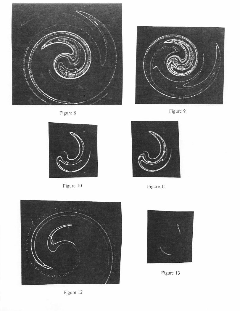
Figure 8 Figure 9

Figure 10 Figure II

Figure 13

Figure 12

o o II 'TS

o CO I II CJxq=—1.5

Vo=2.76

N=12

slope=—1.46

M=4000

eps = .01

12.2 Figure 8 with the Addition of Damping Factor= 0.21

Fig. 9 is the unstable manifold for a fixed point in blue, and the unstablemanifold for a period-two point is green. The data is as follows:

a = —3.0 d = 0.21 Xq = —2.535 2/0 = 5.14

II

00

slope = —0.43 M=1000

eps — .1

a = —3.0 d = 0.21 Xq = —1.465 yo = 2.25 N=16 slope = —1.485 M=2000

eps = .05

The attractor in this case is approximately the point (-2.94,-6.069).


In Fig. 10 the unstable manifold for the fixed point is gone thus this figureis the unstable manifold for a period-two point in green. The data for thisfigure is zs follows:

Period-Two Unstable Manifold (Green):a = -3.0 d = 0.45 a;o = -1.46 yo = 2.285 N=16 slope =-lM M=2000

eps = .03

Fig. 11 is the strange attractor for LT when d = 0.45. The data used ingenerating this figure is as follows:

Strange Attractor (Red):

o CO I II e d=0.45

Xq=—2.535

II N=5000

slope=—1.66

M=1

56


Fig. 12 shows both the unstable manifold (green) for the period-two pointof LT when d = 0.656 and the stable manifold (violet) for this period-twopoint.

The data used in generating this figure is as follows:

o = -3.0 d = 0.656 Xq = —1.4625 yo = 2.022 N=16 slope = —2.0 M=1000

eps = .005

Period-Two Stable Manifold Data (Violet):a = -3.0 d = 0.656 xq =-1.4625 po = 2.022 N=8 slope = 2.0 M=1000

eps = .005

The transverse crossing of the stable and unstable manifolds for LTLTassures us of a horseshoe and thus chaos still persists at this point. We seein the next figure, the strange attractor is clearly in two parts.

Fig. 13 is the strange attractor for LT when d = 0.656. The data used ingenerating this figure is as follows:

Strange Attractor (Red):a = -3.0 d = 0.655 Xq = -1.4625 I yo = 2.022 N=5000 slope = -2.0 M=1

Fig. 13 suggests that it may be possible, through the careful addition ofdamping, to produce homoclinic tangencies in a strange attractor.

12.5 Summary of Section 12

We have seen by the Figures that the fixed-point unstable manifold encasesthe period-two unstable manifold with both manifolds having horseshoes.With damping added, the fixed-point imstable manifold also has between itsfolds areas of the basin of attraction of a fixed-point sink. Prior to the addition of damping, this sink was an elliptic fixed point of FT. The fact that thefixed-point unstable manifold prior to the addition of damping encircled theelliptic region around the elliptic fixed point is significant. This meant thatupon the addition of damping, initial conditions near the fixed-point imstablemanifold could wind up in the basin of attraction of the sink that developed

57

from this elliptic fixed point. In some sense, the outer unstable manifoldprevented chaos from appearing even though it was always possible for somechoices of initial conditions. Once enough damping was added to strip awaythe fixed-point unstable manifold the period-two unstable manifold becamethe attractor. It is likely that this happened because the period-two fixedpoints are on a lower energy curve of the undamped twist than the ellipticfixed point.

We conjecture that this genesis is common to second order square-waveforced nonlinear dynamical systems of the Du£5ng class described in thefollowing section.

13 Concluding Remarks

Crucial to the advancement of any area of scientific research is the presence ofsimple examples on which hypothesis may be tested quickly and efficiently.In this paper we have shown how to construct countless such examples ofsimple transformations that produce chaos. These simple examples differfrom the few predecessors such as the Henon map and the gingerbread map[Devaney, 1984] which existed prior to the twist and flip, in that they arePoincare maps. We consider this "road map" for construction of examplesto be one of our main contributions to the study of chaos.

However, the analysis of the van der Pol and cavitation oscillator equations reveal something more of the genesis of chaos: There appear to be twoprincipal mechanisms for generating a twisting action in autonomous, nonlinear, second order differential equations that can lead to the formation ofchaotic solutions of the equation when a periodic forced is added. We shallrefer to these two classes as the class of Duffing and the class of van derPol/Rayleigh.

Class of Duffing This class is defined by an equation of the form

X-I- V(r) = 0

and

X-I- ai -I- V(x) = 0

where V is a nonlinear function of x, and the first integral of the undampedequation defines a one parameter system of closed curves in the phase plane.

58

Such a system produces a twist or a damped twist and by adding a periodically forcing term to the equation, we may produce a twist or a dampedtwist combined with a flip or some other factor in the Poincare map.

Class of van der Pol/ Rayleigh This dass is defined in two steps:First we consider an equation of the form

5-t-W(i) =0

where W is a nonlinear function of x. The second step in the definition ofthis class is to add a simple linear function of x. We require that the finalequation, which in general looks like

X+ W(x) -j- ax = 0

have a periodic solution. This equation will have a shear action arising fromthe term W(i). The requirement that the solutions be periodic with theaddition of the linear potential term changes this shear into a twist. Theaddition of a periodic forcing term produces a twist factor in the Poincaremap.

These two dasses axe very different physically and the twist factors intheir Poincare maps are also different. We note that in the van der Pol/Rayleighclass the presence of a damping term is essential to produdng the chaos,which is not the case for the Duffing class.

Clearly we may form hybrid equations by combining these two classes ofequations®

We conjecture that a horseshoe twist theorems is true for the Dufi^gclass equations when the periodic forcing term is a square wave if we replacethe circles that play an important role in the horseshoe twist theorem by theclosed curves defined by the first integral. A special case of this conjecturewas presented in [Brown & Chua, 1991].

As for the van der Pol/Rayleigh cleiss, we believe a variation of the horseshoe twist theorem is true for square wave forces, but we do not conjecturethe form of the variation at this time.

The results of this paper suggest numerous questions, but of considerableinterest among all questions that we could ask are two sets.

The first set is concerned with the ergodic properties of the twist andflip, or more generally, the ergodic properties of Poincare maps that are of

®Ueda's form of the van der Pol equation is an example, (Moon, 1987).

59

the form $ o T, where $ is not a twist. Among the questions of interest toengineers and scientist are:

(1) Given the existence of a horseshoe for such a Poincare map, whatare its asjonptotic properties when restricted to the closure of the unstablemanifold, M, which produced the horseshoe?

(2) What are the ergodic factors of such Poincare maps on M.(3) Compute the topological entropy for these maps on M.(4) Classify these maps on M in the categories of weak mixing, strong

mixing, Kolmogorov, or Bernoulli.(5) Since it appears that M could be unbounded, extend the ergodic

concepts to include this case.It should be clear that, in addition to questions of ergodic theory we have

posed, we may also ask many questions about the statistical properties ofthe time series generated by Poincare maps of the form FT or $T.

The second set of questions pertcdn to the harmonic analysis of the chaoticsolutions of the classes of ODEs presented in this paper. In particular, forsquare-wave forcing we can determine the form of the most extreme case ofa chaotic solution of these classes of ODEs by the following considerations.

By the Smale-Birkhoff theorem, some power of the Poincaxe map is tbpo-logically conjugate to a bilateral shift on n-s3niibols on some Cantor set.Therefore, there exist initial conditions in this Cantor set such that the successive iterates of this power of the Poincare map defines a pseudo-randomsequence of points in the plane. Since the forcing is a square wave, thebehavior of the solution between successive points is determined by an autonomous equation whose solutions are periodic functions or spirals. Hencebetween two points of the Poincare map is an arc of such a curve. In the caseof the simple twist this is the arc of a circle. In the case of the undampedDuffing equation it is the arc of a curve defined by the elliptic functions.In any case, the solution of the ODE between two successive iterates of thepower of the Poincare map determined by the Smale-BirkhofF theorem is afinite number of arcs of closed curves or spirals determined by an autonomousODE.

Given this description of the generic chaotic solution of a square-waveforced nonlinear ODE from the classes we have presented we may now construct the simplest example of such a curve and pose some questions aboutits harmonic malysis.

60

Staxting with the one sided shift defined by the equation

®n+i = 2a;n niod 1

on the interval [0,1] we choose an initial condition which generates a densesubset of [0,1]®. This sequence is the analogue of the successive iterates ofthe Poincare map. Next we consider this sequence to define the values ofa function, /, by the rule f{n) = Xn- We now extend the definition of thisfunction, /(t), t > 0, to all positive real numbers by requiring that betweentwo points the function is linear and that the function is continuous for allt > 0. Essentially we are using straight lines in place of the arcs of the closedcurves that appeared in the solution of the ODEs.

If we were to graph such a function we woidd start by plotting the points(n,a;n)» or equivalently, (n,/(n)) in the plane and then we would connecttwo successive points by a straight line. This process produces a boundedcontinuous function. We now ask the following questions about this function:

(1) Does such a function, /(t), have a Fourier transform?(2) What is the power spectral density of / as a function of the initial

condition of the iteration sequence and is the power spectral density continuous?

(3) What questions of spectral synthesis can be answered for such a function?

(4) What does wavelet theory tell us about such a function?Our ability to answer these questions about the function / will determine

to a great extent our ability to deal with chaos through the classical methodsof harmonic analysis.

The twist and flip map has suggested numerous directions of research intothe mechanism of chaos. We now suggest that all of the points we have beenconsidering so far can be formulated in terms of Lie Groups, and that thetwist and flip paradigm can be extended to this setting.

From what has been presented we conclude that the twist and flip ortranslate map is fundamental in producing PBS (Poincar^Birkhoff-Smale)chaos in second order nonlinear periodically forced ODEs and is likely to bethe fundamental paradigm found in many second order ODEs having chaos.

®This sequence should have positive complexity in the sense of Kolmogorov, see [Ford,1986].

61

The strange attractor, as was illustrated in [Brown & Chua, 1991], is alsoaccounted for with this paradigm. The twist and flip map can be extendedto any number of dimensions and may be the key process at work in theequations of Lorenz, Rossler, and in the Chua circuit. We believe the reasonfor the pervasiveness of the twist and flip map as a source of PBS chaos isthat the twist is actually a special case of shearing and the flip is a formof folding. These two actions can be found in the formation of vortices inturbulent flows, a form of chaos, and thus it is not surprising that theyproduce chaos in ODEs.

AcknowledgementsWe thank Professors Morris Hirsch and Charles Pugh of the Department

of Mathematics, University of California, Berkeley for their guidance andtechnical contributions to the work on the horseshoe twist theorem II. Also,we thank Dr. James EUenbogen (MITRE Corporation) for useful suggestionsand conversations and for developing the programs for the Jacobi ellipticfunctions that were used to produce Fig. 4 and to numerically verify conjectures about the elliptic twist and flip maps and their unstable manifolds.

This research is supported in part by the Office of Naval Research undergrant N00014-89-J-1402.

62

List of Figure Captions

Fig. 1 Selected Trajectories from Generalized Twist and Flip Maps whenthe Twist is Defined by a Rotation Function f(r) = I0r/(1 + rlog(r)).

Fig. 2 Selected Trajectories from Generalized Twist and Flip Maps whenthe Twist is Defined by a Rotation Function /(r) = —sin(4log(r)).

Fig. 3 Selected Trajectories from Generalized Twist and Flip Maps whenthe Twist is Defined by a Rotation Function f(r) = (1 + log(r))/r.

Fig. 4 Selected Trajectories from Generalized Twist and Flip Maps whenthe Twist is Defined by a Rotation Function f(r) = —1/r; = l/(r^ + 1)

Fig. 5 Unstable Manifold Used in the Formation of the Smale Horseshoe.

Fig. 6 Seven Forward Iterates of the Square Used in the Formation of theSmale Horseshoe.

Fig. 7 Close-up of the Seventh Forward and Backward Iterate Used in theFormation of the Smale Horseshoe.

Fig. 8 The Fixed-Point Unstable Manifold is in Blue and the Period-TwoUnstable Manifold is in Green. The Two Unstable Manifolds axe Wrappedso Tightly Together that they Give the Illusion of Being Only One UnstableManifold.

Fig. 9 The Fixed-Point Unstable Manifold is in Blue and the Period-TwoUnstable Manifold is in Green. The Addition of Damping Has Contractedthe Unstable Manifolds. The Damping Factor is 0.21 and the Attractor isthe Single Point (—2.94, —6.069).

Fig. 10 The Fixed-Point Unstable Manifold is Gone. The Period-Two Unstable Manifold Remains and is in Green. Sufficient Damping Has Eliminatedthe Fixed-Point Unstable Manifold and Further Contracted the Period-Two

Unstable Manifold. The Damping Factor is 0.45.

Fig. 11 The Attractor for the Damping Factor of 0.45 Appears to be thePeriod-Two Unstable Manifold. The Addition of Damping Has Eliminated

63

the Fixed Point the Attractor in Favor of the Period-Two Unstable Man

ifold. Increased Damping Appears to have Caused the Onset of Chaos.

Fig. 12 The Period-Two Unstable Manifold is Seen in Green and has beenFurther Contracted by Increasing the Damping Factor to 0.656. The StableManifold in Violet Empirically Verifies the Presence of Horseshoes and thusChaos.

Fig. 13 The Period-Two Unstable Manifold Still Appears to be the Attractor Which is Shown in Red. The Damping Factor is 0.656.

65

References

[1] Bois, G. Petit, [1961] Tables of Indefinite Integrals Dover Publications,Inc. Hew York, N. Y.

[2] Brown, Ray, [1990] "An Analytical Test for Chaos", Ph.D. Dissertation,Department of Mathematics, University of California, Berkeley.

[3] Brown, Ray, and Chua, Leon, [1991] "Horseshoes in the Twist and FlipMap", International Journal of Bifurcation and Chaos, Vol. I, Number1, 235-252

[4] Davis, Harold T., \l^^^\Introduction to Nonlinear Differential and Integral Equations. Dover, New York.

[5] Devaney, Robert L., [1984] "A Piecewise Linear Model for the Zones ofInstability of an Area-Preserving Map" Physica lOD, pp. 387-393.

[6] Guckenheimer, J. and Holmes, P.,[1983] Nonlinear Oscillations^ Dynamical Systems, and Bifurcations of Vector Fields. Springer-Verlag, NewYork, N.Y..

[7] Hartman, Philip, [1964] OrdinaryDifferential Equations, John Wiley &Sons, Inc. Assigned Philip Hartman (1973), Baltimore, Md.

[8] Hille, Einar, [1969] Lectures on Ordinary Differential Equations,Addison-Wesley Publishing Company, Menlo Park, Calif.

[9] Hirsch, MorrisW.,[1985] "The Chaos of Dynamical Systems" Publishedin chaos, fractals, and dynamics, P. Fischer and William R. Smith ed..Marcel Dekker, Inc, New York, N.Y..

[10] Hirsch, Morris W. and Pugh, C. C.,[1970]"Stable Manifolds and Hyperbolic Sets",Proc. Symp. Pure Math., Vol 14, AMS, pp.133-163.

[11] Ford, Joseph, [1986] "Chaos: Solving the Unsolvable, Predicting theUnpredictable" from Chaotic Dynamics and Fractals, Academic Press,New York, N. Y.

[12] Ince, E. L, [1956] Ordinary Differential Equations, Dover Publications,New York, N. Y.

66

[13] Moon, Francis C., [1987] Chaotic Vibrations^ John Wiley & Sons, NewYork, N. Y.

[14] Nitecki, Zbigniew [1971] Differentiahle Dynamics, The M.LT. Press,Cambridge, Mass.

[15] Paxlitz, U., Scheffczyk, T., Kurz, T., h Lauterborn, W. [1991]"On Modeling Driven Oscillators by Maps", International Journal of Bifurcationand Chaos, Vol. I, Number 1, 261-264

[16] Smale, S.[1965] "Diffeomorphisms with many periodic points",in Differential and Combinatorial Topology, Princeton University Press, pp.63-80.

[17] Sneddon, I. N., [1957] Elements of Partial Differential Equations,McGraw-Hill, New York

67

Copyright © 1991, by the author(s). All rights reserved ...

Documents

Transcript of Copyright © 1991, by the author(s). All rights reserved ...