Copulas: An Introduction Part II: Models - Columbia Universityrf2283/Conference/2Models (1)...

Copulas: An IntroductionPart II: Models

Johan Segers

Université catholique de Louvain (BE)Institut de statistique, biostatistique et sciences actuarielles

Columbia University, New York City9–11 Oct 2013

Johan Segers (UCL) Copulas. II - Models Columbia University, Oct 2013 1 / 65


Archimedean copulas

Extreme-value copulas

Elliptical copulas

Vines



Archimedean copulas


Elliptical copulas

Vines


The (in)famous Archimedean copulas

I By far the most popular (theory & practice) class of copulasI Plenty of parametric models

I Gumbel, Clayton, Frank, Joe, Ali–Mikhail–Haq, . . .I Building block for more complicated constructions:

I Nested/Hierarchical Archimedean copulasI Vine copulasI Archimax copulasI . . .

I Mindless application of (Archimedean) copulas has drawn manycriticisms on the copula ‘hype’


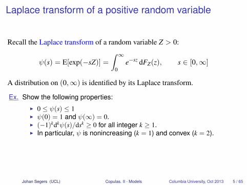
Laplace transform of a positive random variable

Recall the Laplace transform of a random variable Z > 0:

ψ(s) = E[exp(−sZ)] =

∫ ∞0

e−sz dFZ(z), s ∈ [0,∞]

A distribution on (0,∞) is identified by its Laplace transform.

Ex. Show the following properties:

I 0 ≤ ψ(s) ≤ 1I ψ(0) = 1 and ψ(∞) = 0.I (−1)kdkψ(s)/dsk ≥ 0 for all integer k ≥ 1.I In particular, ψ is nonincreasing (k = 1) and convex (k = 2).


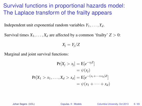
Survival functions in proportional hazards model:The Laplace transform of the frailty appears

Independent unit exponential random variables Y1, . . . ,Yd.

Survival times X1, . . . ,Xd are affected by a common ‘frailty’ Z > 0:

Xj = Yj/Z

Marginal and joint survival functions:

Pr[Xj > xj] = E[e−xjZ]

= ψ(xj)

Pr[X1 > x1, . . . ,Xd > xd] = E[e−(x1+···+xd)Z]

= ψ(x1 + · · ·+ xd)


In proportional hazards models,survival copulas are Archimedean

The survival copula of X is Archimedean with generator ψ:

C(u1, . . . , ud) = ψ(ψ−1(u1) + · · ·+ ψ−1(ud)

)Ex. Show the above formula.

Ex. Show that replacing Z by βZ for a constant β > 0 changes ψ but doesnot change the copula.

Ex. Pick your favourite (discrete/continuous) distribution on (0,∞), computeor look up its Laplace transform, and compute the associatedArchimedean copula. If it doesn’t exist yet, name it after yourself andpublish a paper about it.


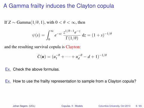
A Gamma frailty induces the Clayton copula

If Z ∼ Gamma(1/θ, 1), with 0 < θ <∞, then

ψ(s) =

∫ ∞0

e−sz z1/θ−1e−z

Γ(1/θ)dz = (1 + s)−1/θ

and the resulting survival copula is Clayton:

C(u) = (u−θ1 + · · ·+ u−θd − d + 1)−1/θ

Ex. Check the above formulas.

Ex. How to use the frailty representation to sample from a Clayton copula?


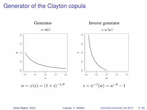
Generator of the Clayton copula

Generator Inverse generator

0.0 0.5 1.0 1.5 2.0

0.0

0.5

1.0

1.5

2.0

w = ψ(s)

s

w

0.0 0.5 1.0 1.5 2.0

0.0

0.5

1.0

1.5

2.0

s = ψ−1(w)

ws

w = ψ(s) = (1 + s)−1/θ s = ψ−1(w) = w−θ − 1


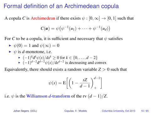
Formal definition of an Archimedean copula

A copula C is Archimedean if there exists ψ : [0,∞]→ [0, 1] such that

C(u) = ψ(ψ−1(u1) + · · ·+ ψ−1(ud)

)For C to be a copula, it is sufficient and necessary that ψ satisfies

I ψ(0) = 1 and ψ(∞) = 0I ψ is d-monotone, i.e.

I (−1)kdkψ(s)/dsk ≥ 0 for k ∈ {0, . . . , d − 2}I (−1)d−2dd−2ψ(s)/dsd−2 is decreasing and convex

Equivalently, there should exists a random variable Z > 0 such that

ψ(s) = E[(

1− sZd − 1

)d−1

+

]i.e. ψ is the Williamson d-transform of the rv (d − 1)/Z.


Standard examples

Ex. The independence copula Π(u) = u1 · · · ud is Archimedean.

I What is its generator ψ?I What is the frailty variable Z?

Ex. The Fréchet–Hoeffding lower bound W(u, v) = max(u + v− 1, 0) isArchimedean too. What is its generator ψ?[This ψ is not a Laplace transform; it is 2-monotone but not d-monotonefor d ≥ 3.]

Ex. One can show that the Fréchet–Hoeffding upper boundM(u) = min(u1, . . . , ud) is not Archimedean. Still, show that the Claytoncopula with θ →∞ converges to M.


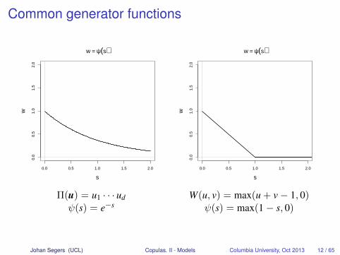
Common generator functions

0.0 0.5 1.0 1.5 2.0

0.0

0.5

1.0

1.5

2.0

w = ψ(s)

s

w

0.0 0.5 1.0 1.5 2.0

0.0

0.5

1.0

1.5

2.0

w = ψ(s)

sw

Π(u) = u1 · · · ud W(u, v) = max(u + v− 1, 0)ψ(s) = e−s ψ(s) = max(1− s, 0)


Bivariate Archimedean copulas as binary operators

A bivariate Archimedean copula induces a binary operator

[0, 1]× [0, 1]→ [0, 1] : (u, v) 7→ C(u, v)

which is commutative and associative:

C(u, v) = C(v, u),

C(u,C(v,w)) = C(C(u, v),w)

endowing [0, 1] with a semi-group structure.

Link with the theory of associative functions (ABEL, HILBERT).


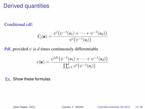
Derived quantities

Conditional cdf:

Cj(u) =ψ′(ψ−1(u1) + · · ·+ ψ−1(ud)

)ψ′(ψ−1(uj)

)Pdf, provided ψ is d times continuously differentiable

c(u) =ψ(d)

(ψ−1(u1) + · · ·+ ψ−1(ud)

)∏dj=1 ψ

′(ψ−1(uj)

)Ex. Show these formulas.


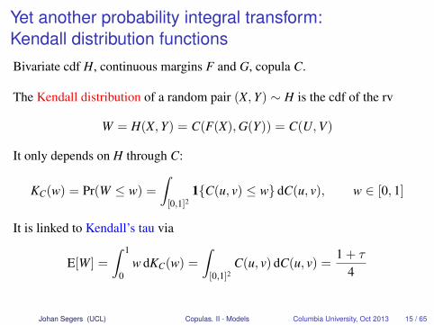
Yet another probability integral transform:Kendall distribution functionsBivariate cdf H, continuous margins F and G, copula C.

The Kendall distribution of a random pair (X,Y) ∼ H is the cdf of the rv

W = H(X,Y) = C(F(X),G(Y)) = C(U,V)

It only depends on H through C:

KC(w) = Pr(W ≤ w) =

∫[0,1]2

1{C(u, v) ≤ w} dC(u, v), w ∈ [0, 1]

It is linked to Kendall’s tau via

E[W] =

∫ 1

0w dKC(w) =

∫[0,1]2

C(u, v) dC(u, v) =1 + τ

4


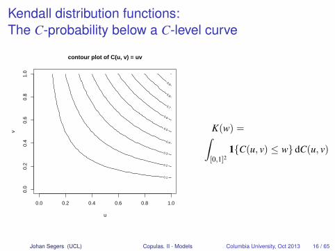
Kendall distribution functions:The C-probability below a C-level curve

contour plot of C(u, v) = uv

u

v

0.1

0.2

0.3

0.4

0.5

0.6

0.7

0.8

0.9

0.0 0.2 0.4 0.6 0.8 1.0

0.0

0.2

0.4

0.6

0.8

1.0

K(w) =∫[0,1]2

1{C(u, v) ≤ w} dC(u, v)


Bivariate Archimedean copulas are identifiedby their Kendall distribution function

The Kendall distribution function of a bivariate Archimedean copula withinverse generator φ = ψ−1 : (0, 1]→ [0,∞) is

K(w) = w− λ(w),

λ(w) =φ(w)

φ′(w)=

1d logφ(w)/dw

≤ 0

Up to a multiplicative constant, φ and thus ψ can be reconstructed from λ.

Ex. Show the following properties:

I KΠ(w) = w− w log(w) (independence)I KW(w) = 1 (Fréchet–Hoeffding lower bound)I KM(w) = w (Fréchet–Hoeffding upper bound)I w ≤ K(w) ≤ 1


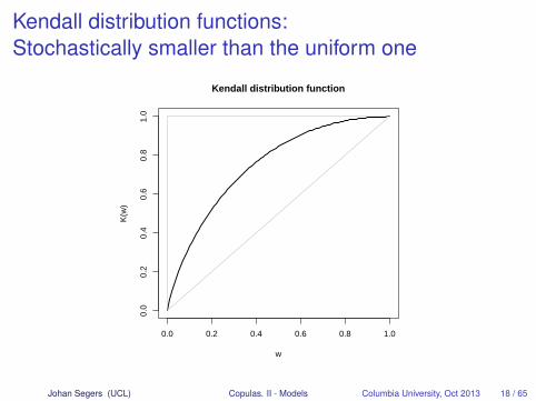
Kendall distribution functions:Stochastically smaller than the uniform one

0.0 0.2 0.4 0.6 0.8 1.0

0.0

0.2

0.4

0.6

0.8

1.0

Kendall distribution function

w

K(w

)


The tail behaviour of a bivariate Archimedean copulacan be read off from the inverse generator function

Coefficient of lower tail dependence:

λL(C) = limw↓0

C(w,w)

w= 2−1/θ0 ,

where θ0 = − limw↓0

wφ′(w)

φ(w)∈ [0,∞]

Coefficient of upper tail dependence:

λU(C) = λL(C) = 2− 21/θ1 ,

where θ1 = − limw↓0

wφ′(1− w)

φ(1− w)∈ [1,∞]

⇒ Construction of models with different upper and lower tails


Archimedean copulas enjoy many symmetries

Let (U1, . . . ,Ud) ∼ C and C is Archimedean with generator ψ.I Permuation symmetry: For any permuation σ of {1, . . . , d},

(Uσ(1), . . . ,Uσ(d))d= (U1, . . . ,Ud)

I Closure of margins: For any subset 1 ≤ j1 < · · · < jk ≤ d,

(Uj1 , . . . ,Ujk) ∼ k-variate Archimedean, same generator ψ

Symmetry is a blessing (simplicity) and a curse (lack of flexibility).

The only radially symmetric Archimedean copula (C = C) is the Frank copula.


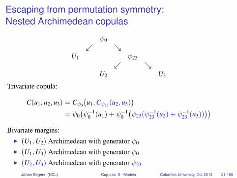
Escaping from permutation symmetry:Nested Archimedean copulas

ψ0↙ ↘

U1 ψ23↙ ↘

U2 U3

Trivariate copula:

C(u1, u2, u3) = Cψ0

(u1,Cψ23(u2, u3)

)= ψ0

(ψ−1

0 (u1) + ψ−10

(ψ23(ψ−1

23 (u2) + ψ−123 (u3))

))Bivariate margins:

I (U1,U2) Archimedean with generator ψ0




Nested Archimedean copulas:Hierarchical dependence structure

U1

U2 U3

U4

U5

U6 U7

D123

D0

D23

D4567

D567

D67

Dependence at deeper levels must be stronger than at higher levels:Sufficient nesting condition on generator functions


Archimedan copulas: Some literature

Alsina, C., M. J. Frank, and B. Schweizer (2006). Associative functions: triangularnorms and copulas. New Jersey: World Scientific.

Charpentier, A. and J. Segers (2009). Tails of multivariate Archimedean copulas.Journal of Multivariate Analysis 2009, 1521–1537.

Genest, C., J. Nešlehová, and J. Ziegel (2011). Inference in multivariateArchimedean copula models. Test 20(2), 223–256.

Genest, C. and L.-P. Rivest (1993). Statistical inference procedures for bivariateArchimedean copulas. Journal of the American Statistical Association 88(423),1034–1043.

McNeil, A. J. and J. Nešlehová (2009). Multivariate Archimedean copulas,d-monotone functions and `1-norm symmetric distributions. The Annals ofStatistics 37(5B), 3059–3097.

Nelsen, R. B. (2006). An Introduction to Copulas. New York: Springer. Chapter 4.Okhrin, O., Y. Okhrin, and W. Schmid (2013). On the structure and estimation of

hierarchical Archimedean copulas. Journal of Econometrics 173(2), 189–204.



Archimedean copulas


Elliptical copulas

Vines


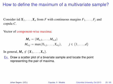
How to define the maximum of a multivariate sample?

Consider iid X1, . . . ,Xn from F with continuous margins F1, . . . ,Fj andcopula C.

Vector of component-wise maxima:

Mn = (Mn,1, . . . ,Mn,d)

Mn,j = max(X1,j, . . . ,Xn,j), j ∈ {1, . . . , d}

In general, Mn 6∈ {X1, . . . ,Xn}.Ex. Draw a scatter plot of a bivariate sample and locate the point

representing the pair of maxima.


The copula of the vector of sample maxima

The joint and marginal cdfs of Mn:

Pr(Mn ≤ x) = Fn(x),

Pr(Mn,j ≤ xj) = Fnj (xj)

The copula of Mn:Cn(u) = C(u1/n

1 , . . . , u1/nd )n

Ex. Prove the above equations.

Ex. If d = 2 and Xi,2 = −Xi,1, we find the Clayton copula with θ = −1/n.


Extreme-value copulas:Limits of copulas of sample maxima

A copula is an extreme-value copula if it can arise in the limit

C∞(u) = limn→∞

C(u1/n1 , . . . , u1/n

d )n

Extreme-value copulas are max-stable:

C∞(u1/k1 , . . . , u1/k

d )k = C∞(u)

Conversely, max-stable copulas are extreme-value copulas.


The only max-stable Archimedean copulais the Gumbel copula

Ex. Show that the Gumbel copula is max-stable:

Cθ(u) = exp[−{(− log u1)θ + · · ·+ (− log ud)θ}1/θ], θ ∈ [1,∞]

Special cases:

θ = 1 Independenceθ =∞ Fréchet–Hoeffding upper bound


Maxima versus minima:Just switch to survival copulas

Everything can be repeated for minima, but the formulas get unwieldyI Apply inclusion/exclusion formulas.

Conceptually, just switch to survival copulas:

C∞ is max/min-stable ⇐⇒ C∞ is min/max-stable

A solution in practice:If interest is in minima, change signs and work with maxima.


The domain of attraction of an extreme-value copula

The (max-)domain of attraction of an extreme-value copula C∞ is thecollection of all copulas C such that

limn→∞

C(u1/n1 , . . . , u1/n

d )n = C∞(u) (DA)

Clearly, C∞ ∈ DA(C∞).

Alternative condition for (DA) in terms of behaviour of C near (1, . . . , 1):

lims↓0

s−1{1− C(1− sx1, . . . , 1− sxd)}

= log C∞(e−x1 , . . . , e−xd ) =: `(x), x ∈ [0,∞)d

The limit is called the stable tail dependence function.[Proof: In (DA), take logarithms and set s = 1/n and uj = e−xj .]


Archimedean copulas:Attracted by the Gumbel copula

If C is Archimedean with inverse generator φ = ψ−1 and if

∃ limw↓0−wφ′(1− w)

φ(1− w)= θ1 ∈ [1,∞]

then C ∈ DA(Gumbel copula Cθ1).

Ex. Show that the Joe copula with inverse generator

φθ(w) = − log(1− (1− w)θ

), θ ∈ [1,∞),

is attracted by the Gumbel copula with parameter θ.


Archimedean survival copulas:Attracted by the Galambos copulaIf C is Archimedean with inverse generator φ = ψ−1 and if

∃ limw↓0−wφ′(w)

φ(w)= θ0 ∈ [0,∞]

then C ∈ DA(Galambos copula Cθ0), with stdf

`θ(x) = x1 + · · ·+ xd −∑

I⊂{1,...,d},|I|≥2

(−1)|I|(∑

j∈J x−θj

)−1/θ

Ex. Show that the survival Clayton copula with inverse generator

φθ(w) =w−θ − 1

θ, θ ∈ [0,∞),

is attracted by the Galambos copula with the same parameter.


Pickands dependence functions:A kind of generator function on the unit simplex

If C∞ is max-stable, the function A on

∆d−1 = {t ∈ [0, 1]d : t1 + · · ·+ td = 1}

defined by

A(t) =log C∞(wt1 , . . . ,wtd )

log w

does not depend on w ∈ (0, 1). We find the Pickands representation

C∞(wt1 , . . . ,wtd ) = wA(t)


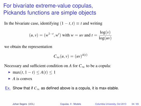
For bivariate extreme-value copulas,Pickands functions are simple objects

In the bivariate case, identifying (1− t, t) ≡ t and writing

(u, v) = (w1−t,wt) with w = uv and t =log(v)

log(uv)

we obtain the representation

C∞(u, v) = (uv)A(t)

Necessary and sufficient condition on A for C∞ to be a copula:I max(t, 1− t) ≤ A(t) ≤ 1I A is convex

Ex. Show that if C∞ as defined above is a copula, it is max-stable.


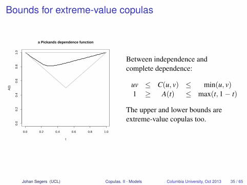
Bounds for extreme-value copulas

0.0 0.2 0.4 0.6 0.8 1.0

0.0

0.2

0.4

0.6

0.8

1.0

a Pickands dependence function

t

A(t

)

Between independence andcomplete dependence:

uv ≤ C(u, v) ≤ min(u, v)1 ≥ A(t) ≤ max(t, 1− t)

The upper and lower bounds areextreme-value copulas too.


Extreme-value copulas:An abundance of parametric models

Ex. Look up the forms of the following extreme-value copulas andvisualize their Pickands dependence functions:

I Gumbel aka logistic, and asymmetric extensionsI Galambos aka negative logistic, and asymmetric extensionsI Marshall–OlkinI Hüsler–ReissI t-EVI SchlatherI . . .


Extreme-value copulas:Flexible models for positively associated variables

I Kendall’s tau:

τ =

∫ 1

0

t(1− t)A(t)

dA′(t) > 0 unless independence

I Coefficient of upper tail dependence:

λU = 2(1− A(1/2)

)> 0 unless independence

I Not necessarily symmetricI Higher dimensions: hierarchical structures possibleI Margins of extreme-value copulas are also extreme-value copulas


Extreme-value copulas: Some literature I

Beirlant, J., Y. Goegebeur, J. Segers, and J. Teugels (2004). Statistics of Extremes:Theory and Applications. Chichester: Wiley. Chapters 8 and 9.

Bücher, A., H. Dette, and S. Volgushev (2011). New estimators of the Pickandsdependence function and a test for extreme-value dependence. The Annals ofStatistics 39(4), 1963–2006.

Fougères, A., J. Nolan, and H. Rootzén (2009). Models for dependent extremes usingstable mixtures. Scandinavian Journal of Statistics 36, 42–59.

Genest, C., I. Kojadinovic, J. Nešlehová, and J. Yan (2011). A goodness-of-fit test forextreme-value copulas. Bernoulli 17, 253–275.

Genest, C. and J. Segers (2009). Rank-based inference for bivariate extreme-valuecopulas. The Annals of Statistics 37(5B), 2990–3022.

Gudendorf, G. and J. Segers (2010). Extreme-value copulas. In W. H. P. Jaworski,F. Durante and T. Rychlik (Eds.), Proceedings of the Workshop on Copula Theoryand its Applications, Berlin, pp. 127–146. Springer.

Gudendorf, G. and J. Segers (2012). Nonparametric estimation of multivariateextreme-value copulas. Journal of Statistical Planning and Inference 142,373–385.


Extreme-value copulas: Some literature II

Guillotte, S. and F. Perron (2008). A Bayesian estimator for the dependence functionof a bivariate extreme-value distribution. The Canadian Journal of Statistics 36(3),383–396.

Kojadinovic, I., J. Segers, and J. Yan (2011). Large-sample tests of extreme-valuedependence for multivariate copulas. The Canadian Journal of Statistics 39,703–720.

Peng, L., L. Qian, and J. Yang (2013). Weighted estimation of the dependencefunction for an extreme-value distribution. Bernoulli 19(2), 492–520.

Zhang, D., M. T. Wells, and L. Peng (2008). Nonparametric estimation of thedependence function for a multivariate etreme value distribution. Journal ofMultivariate Analysis 99(4), 577–588.



Archimedean copulas


Elliptical copulas

Vines


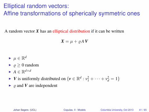
Elliptical random vectors:Affine transformations of spherically symmetric ones

A random vector X has an elliptical distribution if it can be written

X = µ+ %A V

I µ ∈ Rd

I % ≥ 0 randomI A ∈ Rd×d

I V is uniformly distributed on {v ∈ Rd : v21 + · · ·+ v2

d = 1}I % and V are independent


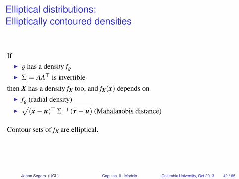
Elliptical distributions:Elliptically contoured densities

IfI % has a density f%I Σ = AA> is invertible

then X has a density fX too, and fX(x) depends onI f% (radial density)I√

(x− u)>Σ−1 (x− u) (Mahalanobis distance)

Contour sets of fX are elliptical.


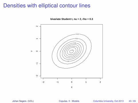
Densities with elliptical contour lines

bivariate Student t, nu = 2, rho = 0.3

X

Y 0.02

0.04

0.06

0.08

0.1

0.12

0.14

0.16

−2 −1 0 1 2

−2

−1

01

2


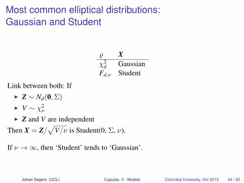
Most common elliptical distributions:Gaussian and Student

% Xχ2

d GaussianFd,ν Student

Link between both: IfI Z ∼ Nd(0,Σ)

I V ∼ χ2ν

I Z and V are independent

Then X = Z/√

V/ν is Student(0, Σ, ν).

If ν →∞, then ‘Student’ tends to ‘Gaussian’.


Meta-elliptical copulas:Copulas of elliptical distributions

A copula is meta-elliptical if it is the copula of an elliptical distribution.

A meta-elliptical copula is itself not an elliptical distribution.Hence ‘meta’; suppressed in practice.

Without loss of generality, we can assume thatI µ = 0I Σ is a correlation matrix, notation R

Ex. Why?


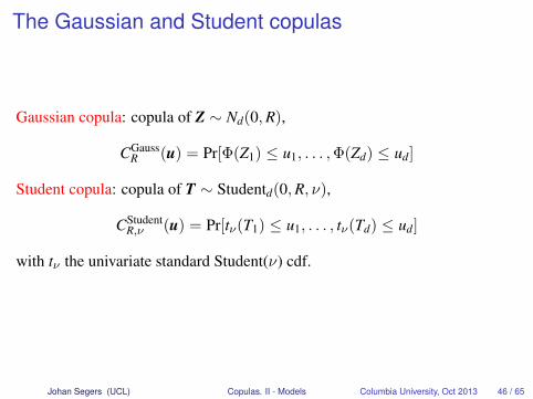
The Gaussian and Student copulas

Gaussian copula: copula of Z ∼ Nd(0,R),

CGaussR (u) = Pr[Φ(Z1) ≤ u1, . . . ,Φ(Zd) ≤ ud]

Student copula: copula of T ∼ Studentd(0,R, ν),

CStudentR,ν (u) = Pr[tν(T1) ≤ u1, . . . , tν(Td) ≤ ud]

with tν the univariate standard Student(ν) cdf.


Elliptical copula densities:Contour lines are not elliptical

bivariate Student t copula, nu = 2, rho = 0.3

u

v

1 1

1

2

2

3 4

0.0 0.2 0.4 0.6 0.8 1.0

0.0

0.2

0.4

0.6

0.8

1.0

u

v

c(u, v)

bivariate Student t copula, nu = 2, rho = 0.3


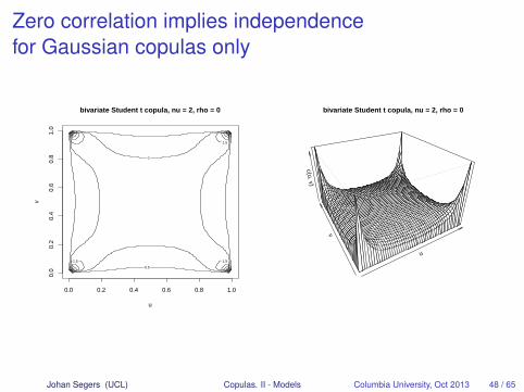
Zero correlation implies independencefor Gaussian copulas only

bivariate Student t copula, nu = 2, rho = 0

u

v

0.5

1

1.5

1.5

1.5

1.5

2 2

2

0.0 0.2 0.4 0.6 0.8 1.0

0.0

0.2

0.4

0.6

0.8

1.0

u

v

c(u, v)

bivariate Student t copula, nu = 2, rho = 0


Elliptical copulas are convenient to work with

I Densities are explicitly available.I Pairwise distributions determine the full distribution.I Lower-dimensional margins are elliptical copulas again.I If U ∼ C is elliptical, then, whatever the radial distribution,

τ(Uj,Uk) =arcsin(rjk)

π/2(Kendall’s tau)

I Tail dependence follows from power-law tail of %, e.g.I Gaussian copula: asymptotic independenceI Student copula: λL = λU = 2 tν+1(−

√(ν + 1)(1− ρ)/(1 + ρ))


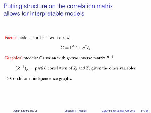
Putting structure on the correlation matrixallows for interpretable models

Factor models: for Γk×d with k < d,

Σ = Γ′Γ + σ2Id

Graphical models: Gaussian with sparse inverse matrix R−1

(R−1)jk = partial correlation of Zj and Zk given the other variables

⇒ Conditional independence graphs.


Elliptical copulas: Some literature

Demarta, S. and A. J. McNeil (2005). The t copula and related copulas. InternationalStatistical Review 73(1), 111–129.

Fang, H.-B., K.-T. Fang, and S. Kotz (2002). The meta-elliptical distributions withgiven marginals. Journal of Multivariate Analysis 82, 1–16.

Genest, C., A.-C. Favre, J. Béliveau, and C. Jacques (2007). Metaelliptical copulasand their use in frequency analysis of multivariate hydrological data. WaterResources Research 43, W09401.

Hult, H. and F. Lindskog (2002). Multivariate extremes, aggregation and dependencein elliptical distributions. Adv. Appl. Probab. 34, 587–608.

Klüppelberg, C. and G. Kuhn (2009). Copula structure analysis. Journal of the RoyalStatistical Society: Series B (Statistical Methodology) 71(3), 737–753.



Archimedean copulas


Elliptical copulas

Vines


The simplifying assumption:The copula of a conditional distribution

For random variables (X,Y) and a random vector Z, assume:

The copula of (X,Y) | Z = z does not depend on z.

Equivalently, assume:

(FX|Z(X | Z),FY|Z(Y | Z)) is independent of Z.

I True if (X,Y,Z) are jointly GaussianI (X,Y) | Z = z is bivariate GaussianI Conditional correlation is partial correlation ρXY·Z, whatever z

I Simplifying assumption not verified in general


From the simplifying assumption to vine copulas

Vine copulas or pair-copula constructions:Combine d(d − 1)/2 arbitrary bivariate copulas into a d-variate copula.

I The bivariate copulas are not the bivariate margins.I They rather arise through repeated conditioning.I Construction made possible by the simplifying assumption.


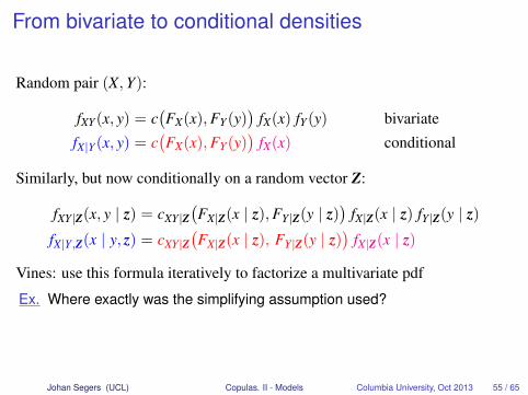
From bivariate to conditional densities

Random pair (X,Y):

fXY(x, y) = c(FX(x),FY(y)

)fX(x) fY(y) bivariate

fX|Y(x, y) = c(FX(x),FY(y)

)fX(x) conditional

Similarly, but now conditionally on a random vector Z:

fXY|Z(x, y | z) = cXY|Z(FX|Z(x | z),FY|Z(y | z)

)fX|Z(x | z) fY|Z(y | z)

fX|Y,Z(x | y, z) = cXY|Z(FX|Z(x | z), FY|Z(y | z)

)fX|Z(x | z)

Vines: use this formula iteratively to factorize a multivariate pdf

Ex. Where exactly was the simplifying assumption used?


Vines in dimension threeTaking X3 as ‘pivot’ variable:

f (x1, x2, x3)

= f3(x3)

f2|3(x2|x3)

f1|23(x1|x2, x3)

= f3(x3)

c23(F2(x2),F3(x2)

)f2(x2)

c12|3(F1|3(x1|x3), F2|3(x2|x3)

)f1|3(x1|x3)︸︷︷︸

=c13(F1(x1),F3(x3)) f1(x1)

= f1(x1) f2(x2) f3(x3)

c13(F1(x1), F3(x3)

)c23(F2(x2), F3(x2)

)c12|3

(F1|3(x1|x3)︸︷︷︸

=?

, F2|3(x2|x3))


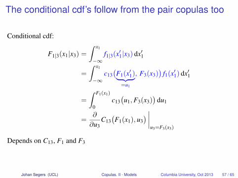
The conditional cdf’s follow from the pair copulas too

Conditional cdf:

F1|3(x1|x3) =

∫ x1

−∞f1|3(x′1|x3) dx′1

=

∫ x1

−∞c13(F1(x′1)︸︷︷︸=u1

, F3(x3))

f1(x′1) dx′1

=

∫ F1(x1)

0c13(u1,F3(x3)

)du1

=∂

∂u3C13(F1(x1), u3

) ∣∣∣∣u3=F3(x3)

Depends on C13, F1 and F3


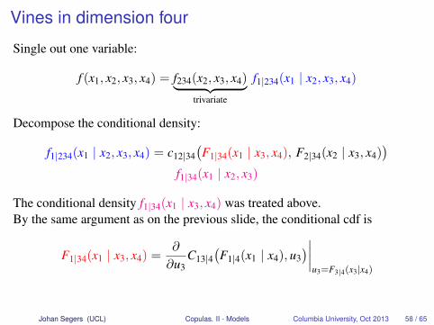
Vines in dimension four

Single out one variable:

f (x1, x2, x3, x4) = f234(x2, x3, x4)︸︷︷︸trivariate

f1|234(x1 | x2, x3, x4)

Decompose the conditional density:

f1|234(x1 | x2, x3, x4) = c12|34(F1|34(x1 | x3, x4), F2|34(x2 | x3, x4)

)f1|34(x1 | x2, x3)

The conditional density f1|34(x1 | x3, x4) was treated above.By the same argument as on the previous slide, the conditional cdf is

F1|34(x1 | x3, x4) =∂

∂u3C13|4

(F1|4(x1 | x4), u3

)∣∣∣∣u3=F3|4(x3|x4)


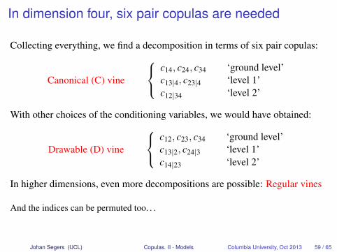
In dimension four, six pair copulas are needed

Collecting everything, we find a decomposition in terms of six pair copulas:

Canonical (C) vine

c14, c24, c34 ‘ground level’c13|4, c23|4 ‘level 1’c12|34 ‘level 2’

With other choices of the conditioning variables, we would have obtained:

Drawable (D) vine

c12, c23, c34 ‘ground level’c13|2, c24|3 ‘level 1’c14|23 ‘level 2’

In higher dimensions, even more decompositions are possible: Regular vines

And the indices can be permuted too. . .


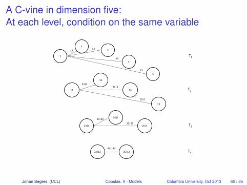
A C-vine in dimension five:At each level, condition on the same variable

1

2 3

4

5

T1 12 13

14

15

12

13

14

15

T2 23|1

24|1

25|1

23|1

24|1

25|1 T3 34|12

35|12

34|12 35|12 T4 45|123


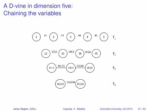
A D-vine in dimension five:Chaining the variables


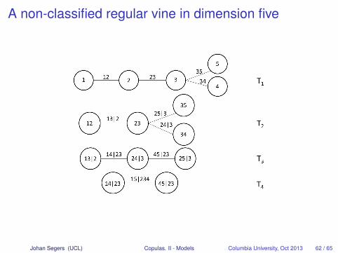
A non-classified regular vine in dimension five


Vine copulas: Strengths

I Densities are explicitI Conditioning mechanism also yields simulation algorithmsI Models are easily constructed: any pair copula worksI Highly flexible

I asymmetriesI positive/negative dependenceI tail dependence


Vine copulas: Weaknesses

I Cdf’s not explicitly availableI Taking margins destroys the modelI Meaning of chain of simplifying assumptions is not transparentI Interpretation becomes difficult


Vine copulas: Some literatureActive and fast-moving field. Check out

http://www-m4.ma.tum.de/forschung/vine-copula-models/

Aas, K., C. Czado, A. Frigessi, and H. Bakken (2009). Pair-copula constructions ofmultiple dependence. Insurance: Mathematics & Economics 44(2), 182–198.

Bedford, T. and R. M. Cooke (2002). Vines—a new graphical model for dependentrandom variables. The Annals of Statistics 30(4), 1031–1068.

Brechmann, E. and U. Schepsmeier (2013). Modeling dependence with C- andD-vine copulas: the R package CDVine. Journal of Statistical Software 52(3),1–27.

Hobæk Haff, I. (2013). Parameter estimation for pair-copula constructions.Bernoulli 19(2), 462–491.

Joe, H. (1996). Families of m-variate distributions with given margins andm(m− 1)/2 bivariate dependence parameters. In Distributions with fixedmarginals and related topics (Seattle, WA, 1993), Volume 28 of IMS Lecture NotesMonogr. Ser., pp. 120–141. Hayward, CA: Inst. Math. Statist.


http://www-m4.ma.tum.de/forschung/vine-copula-models/

Copulas: An Introduction Part II: Models - Columbia Universityrf2283/Conference/2Models (1)...

Documents

Transcript of Copulas: An Introduction Part II: Models - Columbia Universityrf2283/Conference/2Models (1)...