CopulaDTA: An R package for copula-based

bivariate beta-binomial models for diagnostic

test accuracy studies in Bayesian framework

Victoria Nyaga1,2, Marc Arbyn2, Marc Aerts1.

May 18, 2016

1. Universiteit Hasselt.

2. Scientific Institute of Public Health.

Introduction

Normal Squamous

Cells (~93%)

Atypical squamous cells

LSIL HSIL(~4%) Cancer (~1%)

1

Introduction

Normal Squamous

Cells (~93%)

Atypical squamous cells

LSIL

HSIL(~4%)

Cancer (~1%)

Triage group

Routine check-up every 3 years

?Repeat pap smear

? HPV DNA Testing

?HPV Mrna testing

?...

Further exploration and treatment

Surgery

Radiotherapy

...

Management

Prediction on natural history difficult

Spontaneous regression

Anxiety

Invasive treatment

Financial burden

Discomfort

Overdiagnosis

Overtreatment

Prevention

Increased survival

Implication(s)

2

Research interest

Diagnostic tests identifying women whose cervical lesions confer increased

risk of cervical cancer.

Arbyn et al. (2013)

Among ASCUS triage group determine;

• Accuracy of

1. HPV DNA Testing using HC2, and

2. Repeat cytology in detecting CIN2+.

• Differences in accuracy between the two triage tests.

3

Hypothetical data

Study 1

Study 2

Study 3

Study 4

Study 5

… N

4

Goal

• Obtain population-averaged estimates.

• Account for the present intrinsic correlation between sensitivity and

specificity.

• Obtain forest plots.

5

Outline

1. Bivariate normal vs. beta random-effects

2. The CopulaDTA package

3. Application

6

Bivariate normal vs. beta random-effects

TPi | sei , xi ∼ bin(sei , Disi ), i = 1, . . . N,

TNi | spi , xi ∼ bin(spi , NonDisi ), i = 1, . . . N.

Normal distribution

(logit(sei )

logit(spi )

)∼ N

((µlogitse

µlogitsp

),Σ

)

Σ =

[σ2

1 ρσ1σ2

ρσ1σ2 σ22

]

Beta distribution

(seispi

)∼ f (sei )f (spi )c(F (sei ),F (spi ), θ)

f(sei ) = Beta(µse , ψse),

f(spi ) = Beta(µsp, ψsp),

c(.) = copula density: frank, gaussian, ...

µ. = logit−1(ν.) = α.

(α.+β.)

ψ. = (α. + β.) or 11+α.+β.

7

Bivariate normal vs. beta random-effects

Normal distribution

• Availability of software; SAS, R,...

• Approximative distribution:

• Large sample size.

• (µlogitse

µlogitsp

)

• Expit transformation(µse |εlogitse = 0

µsp|εlogitsp = 0

)• (

µse

µsp

)=

(E(logit−1(µlogitse + εlogitse))

E(logit−1(µlogitsp + εlogitsp))

)

Beta bistribution

• Programming

skills needed: R,

JAGS, STAN, ...

• Natural choice

• (µse

µsp

)

8

CopulaDTA package

MCMC sampling engine

Stan

1. Easy to extend compared to JAGS(.dll).

functions {}data {}transformed data {}parameters {}transformed parameters {}model {}generated quantities {}

2. Faster convergence with fewer iteration even with poor initial values

than with JAGS.

9

CopulaDTA package

Functions, objects and methods

• cdtamodel function → cdtamodel object

R > model < - cdtamodel(copula = ’fgm’,

+ modelargs=list(formula.se = StudyID ∼ Test - 1,

+ formula.sp = StudyID ∼ Test - 1,

+ formula.omega = StudyID ∼ Test - 1,

+ param=2,

+ prior.lse=’normal’, par.lse1=0, par.lse2=5,

+ prior.lsp=’normal’, par.lsp1=0, par.lsp2=5,...))

• fit function → cdtafit object

R >fitmodel <- fit(cdtamodel object, data, SID, cores=3,chains=3,

+ iter=6000, warmup=1000,thin=10, ...)

• Methods for cdtafit object: print, summary, plot, str

10

Application

Package Installation

R> install.packages(”CopulaDTA”, dependencies = TRUE)

R> library(CopulaDTA)

Data

R> data(ascus)

R> ascus

Test StudyID TP FP TN FN

RepC Anderson 2005 6 14 28 4

RepC Bergeron 2000 8 28 71 4

RepC Del Mistro 2010 20 191 483 7

. . . . . .

HC2 Silverloo 2009 34 65 81 2

HC2 Solomon 2001 256 1050 984 11

11

Application

Model fitting

R> frank <- cdtamodel(copula = “frank”,

+ modelargs = list(formula.se = StudyID ∼ Test + 0))

R> fitfrank <- fit(frank,

+ data = ascus,

+ SID = “StudyID”,

+ iter = 19000,

+ warmup = 1000,

+ thin = 20,

+ seed = 3)

12

Application

Posterior Estimates

R > print(fitfrank, digits=4)

13

Application

Forest Plot

R > plot(fitfrank)

Sensitivity Specificity

● ●

● ●

● ●

● ●

● ●

● ●

● ●

● ●

● ●

● ●

● ●

●●

● ●

●●

●●

●●

●●

● ●

●●

●●

Overall

Solomon 2001

Silverloo 2009

Morin 2001

Monsonego 2008

Manos 1999

Lytwyn 2000

Kulasingam 2002

Del Mistro 2010

Bergeron 2000

Andersson 2005

0.00 0.25 0.50 0.75 1.00 0.00 0.25 0.50 0.75 1.00

Stu

dyID

Test ● ●HC2 RepC

Plot of study−specific posterior sensitivity and specificity byStudyID and Test: marginal mean and 95% CI

14

Summary

• Repeat cytology less sensitive than HC2 in diagnosing cervical

precancer in women with equivocal pap smear.

• Marginal as well as study-specific estimates.

• Parameters with natural interpretation.

15

References

Arbyn M, Roelens J, Simoens C, Buntinx F, Paraskevaidis E,

Martin-Hirsch PP, Prendiville WJ (2013).

“Human Papillomavirus Testing Versus Repeat Cytology for

Triage of Minor Cytological Cervical Lesions.”

Cochrane Database of Systematic Reviews, 31–201.

Reitsma JB, Glas AS, Rutjes AW, Scholten RJ, Bossuyt PM,

Zwinderman AH (2005).

“Bivariate Analysis of Sensitivity And Specificity Produces

Informative Summary Measures in Diagnostic Reviews.”

Journal of Clinical Epidemiology, 58(10), 982–990.

Nyaga VN (2015).

CopulaDTA: Copula Based Bivariate Beta-Binomial Model for

Diagnostic Test Accuracy Studies.R package version 0.0.2,

URL http://CRAN.R-project.org/package=CopulaDTA.

16

Good evening

&

Enlightening conference

16

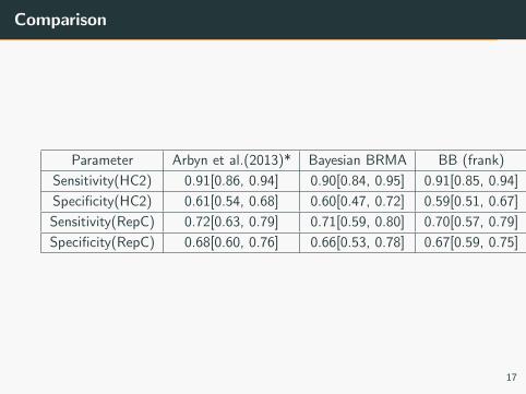
Comparison

Parameter Arbyn et al.(2013)* Bayesian BRMA BB (frank)

Sensitivity(HC2) 0.91[0.86, 0.94] 0.90[0.84, 0.95] 0.91[0.85, 0.94]

Specificity(HC2) 0.61[0.54, 0.68] 0.60[0.47, 0.72] 0.59[0.51, 0.67]

Sensitivity(RepC) 0.72[0.63, 0.79] 0.71[0.59, 0.80] 0.70[0.57, 0.79]

Specificity(RepC) 0.68[0.60, 0.76] 0.66[0.53, 0.78] 0.67[0.59, 0.75]

17

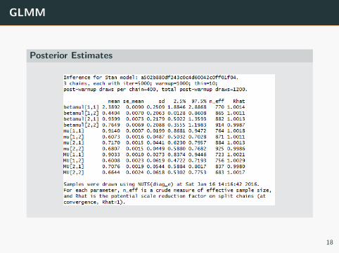
GLMM

Posterior Estimates

18