Copula functions and bivariate distributions for survival

analysis: An application to political survival

Alejandro Quiroz Flores

Wilf Department of Politics

New York University

19 West 4th St, Second Floor

New York, NY 10012-1119

aqf200@nyu.edu

July 20, 2008

Abstract

Event-history analysis often focuses on the survival time of a single subject. However,

recent research in the social sciences demands estimation of the joint survival time of different

subjects. This paper presents a method to estimate the interdependence between two different

subjects. Analogous to seemingly unrelated regressions (SUR) or bivariate probit models, this

paper begins with the assumption that the two different survival processes are not independent.

The interdependence between processes is modelled as part of a bivariate distribution suit-

able for survival analysis, such as the bivariate exponential and the bivariate Weibull. These

bivariate distributions are derived from copula functions. To test the performance of these dis-

tributions, the paper presents a simulation experiment. In order to illustrate these methods, the

paper presents an application to a new data set on the tenure of leaders and foreign ministers.

1

1 Introduction

Event-history analysis often focuses on the survival time of a single subject. However, recent re-

search in the social sciences demands estimation of the joint survival time of different subjects.

This paper presents a method to estimate the interdependence between two different subjects.

Analogous to seemingly unrelated regressions (SUR) or bivariate probit models, this paper begins

with the assumption that the two different survival processes are not independent. The interde-

pendence between processes is modelled as part of a bivariate distribution suitable for survival

analysis, such as the bivariate exponential and the bivariate Weibull. These bivariate distributions

are derived from copula functions. Copula functions are a flexible and powerful method to pro-

duce and analyze large classes of multivariate distributions. These functions are the cornerstone of

multivariate analysis since they allow for the construction of previously unknown bivariate distri-

butions by using known marginals.

To test the performance of these distributions, the paper presents a simulation experiment. The

experiment simulates data from bivariate Weibull distributions according to different degrees of

interdependence between survival processes, and then estimates the parameters from bivariate and

univariate Weibull distributions. The results from estimation suggest that when there is strong in-

terdependence between the survival processes, the bivariate distribution performs much better than

the univariate distribution. In cases of weak interdependence, the bivariate distribution performs

as well as the univariate distribution. Therefore,given the simplicity in estimating a bivariate

Weibull, and regardless of the degree of interdependence between processes, it is recommended

that the parameters from this distribution are chosen over the parameters of a univariate Weibull.

The interdependent nature of survival processes is ubiquitous in insurance, economics, finance,

political science, and sociology, among other fields. For example, the length of time an individual

stays in a marriage might affect the time that individual stays in her job and viceversa. In politics,

it is usually the case that the tenure of a cabinet minister and the tenure of a prime minister are

interdependent. Political institutions define the degree and direction of this interdependence. Based

2

on this hypothesis, and as an illustration of the methods described above, the paper estimates

the joint survival time of leaders and ministers of foreign affairs. The estimation is based on a

completely new political science data set that comprises the tenure of more than 7,000 foreign

ministers in 181 countries, spanning three centuries.

The paper begins with a revision of existing research on survival analysis and multivariate

distributions. The second section presents an introduction to copula functions as a method to

produce bivariate distributions. The third part of the paper describes a bivariate exponential and a

bivariate Weibull. These functions are the workhorses of survival analysis. In the fourth section,

the paper discusses the technique used for the estimation of the parameters of the aforementioned

distributions. In order to study the properties of the proposed estimators, the fifth section presents

a simulation experiment. In the final section, the paper applies these methods to the joint survival

of leaders and foreign ministers.

2 Background

Consider two different survival timest1 andt2. Each of them depends on some covariates and a

particular disturbance.

t1 = f(X, ε1). (1)

t2 = f(Z, ε2). (2)

Instead of assuming that each of these processes comes from a marginal distribution like an expo-

nential or a Weibull, this paper assumes that they come from a bivariate distribution. Models like

the SUR and the bivariate probit are based on the assumption of normality. Indeed, the use of a bi-

variate normal presents no serious complications for maximum likelihood estimation. In survival

analysis, however, the central methodological issue resides on the development of non-normal

multivariate distributions and the generation of numbers from those distributions.

3

Several methods have been used extensively to produce multivariate distributions, such as con-

ditional distributions, mixing distributions, and inversion methods. Several authors have devel-

oped different procedures to derive multivariate or bivariate distributions (Gumbel 1960; Hougaard

1986; Johnson 1986; Johnson, Evans, and Green 1999). In political science, most of the methods

have been limited to solving specific problems like selection bias (Boehmke, Morey, and Shan-

non 2006), competing risks (Gordon 2002), or government formation (Hays and Kachi 2008).

Moreover, with the exception of Gordon (2002), most research in political science uses statistical

programs that have important limitations for simulation and estimation. Given the lack of coher-

ence in the derivation of multivariate distributions, one alternative resides on the estimation of

discrete survival models (Beck, Katz, and Tucker 1998). For instance, we can use a bivariate pro-

bit to estimate the joint hazard rate of two different subjects. The bivariate probit (Greene 2003;

Van de Ven and Van Pragg 1981) is a well-known model, and it is the basis of other models that

address interdependent failure events (Petersen 1995). Moreover, Maddala (1983) has proposed a

two-stage simultaneous equation probit model that may also be useful.

This paper contributes to this research by developing general continuous survival models that

have extensive applications in political science and other fields. Moreover, instead of focusing on

the details of a single distribution, this paper describes how to derive bivariate distributions. The

method is based on copula functions, which are a flexible and powerful method to produce and

analyze large classes of multivariate distributions. These distributions are necessary to estimate

the parameters that govern interdependent processes. This method is relatively new in the statistics

literature and almost completely unknown in political science. For instance, Gumbel’s extensively

used bivariate exponential (1960) is a special case of bivariate distributions based on copula func-

tions. Indeed, we can have a better understanding of the behavior of this and other distributions by

looking at them as the result of copulas.

4

3 Copula functions

A thorough description of copula functions, as well as the proofs of the main theorems, is beyond

the scope of this article. Such studies of copula functions can be found elsewhere (e.g. Nelsen

2006; Trivedi and Zimmer 2005). The purpose of this section is to introduce copula functions to

political science by summarizing the main theorems and results derived in the last 50 years.

Copulas are functions that join multivariate distribution functions to their one-dimensional

marginal distribution functions.1 Suppose there are two random variablesX andY with cumula-

tive distribution functionsF (x) andG(y) respectively. According toSklar’s Theorem, there exists

a copulaC such that, for allx andy in the extended real line, there is a joint distribution function

H(x, y) = C[F (x), G(y)]. This theorem suggests that a bivariate distribution can be expressed as

a function of marginal distributions. That particular function is a copula that fulfills certain condi-

tions and that can be parameterized to include a measure of dependence between marginals. The

theorem is a cornerstone of multivariate analysis since it allows for the construction of previously

unknown bivariate distributions by using known marginals.

A copula function must fulfill important conditions.A two-dimensional subcopula is a function

C ′ with the following properties. (1) The domain ofC ′ is S1 × S2, whereS1 andS2 are subsets of

I = [0, 1]. (2)C ′ is grounded and 2-increasing. (3) For everyu in S1 andv in S2, thenC ′(u, 1) = u

andC ′(1, v) = v. A two-dimensional copula is a subcopula C whose domain isI2.

The first characteristic of a copula function suggests that its cumulative distribution function

(CDF) is confined to the unit cube. This is true since each marginal distribution has a CDF with

a range between 0 and 1. This means thatF (x) andG(y) are subsets ofI = [0, 1]. The domain

of the bivariate function is thus given by the Cartesian product of the two cumulative marginals.

This results in a bivariate CDF with a range between 0 and 1. However, the function could be

even more constrained. These constraints are given by the Frechet-Hoeffding bounds inequality:

1Most of the definitions, conditions, and notation throughout the paper are borrowed from Nelsen (2006).

5

max[F (x) + G(y)− 1, 0] ≤ C ′(x, y) ≤ min[F (x), G(y)].

The second characteristic of a copula suggests that, in a three-dimensional perspective, the

function is non-decreasing. A two-dimensional function is2-increasingif the volume of a Carte-

sian product in its domain is always greater than or equal to 0. In other words, this means that if

the CDF of the bivariate distribution has a second derivative, then the derivative in respect to the

two margins is greater than or equal to 0. The function isgroundedif its value is equal to 0 at the

minimum value of one of its margins, for all possible values of the other margin. This means that

if the probability of any outcome is 0, that is, if a marginal is equal to 0, then the joint probability

of all outcomes is 0 as well.

Copula functions do not focus on correlation coefficients but on scale invariantmeasures of as-

sociation. It is important to highlight that these measures of association are a function of a measure

of dependence between marginals. Thismeasure of dependence, also known as an association pa-

rameter, is denotedθ. The measure of dependence can take on many different values depending on

the copula, whereas measures of association, such as Pearson’s correlation coefficient, are usually

bounded. In many cases,θ will further constrain a correlation coefficient. This is a serious problem

for some distributions, like Gumbel’s bivariate exponential, which can only handle a correlation

within the [-.25, .25] interval. However, other distributions like the bivariate Weibull allow for

larger correlation coefficients. The next section presents an illustration of the relationship between

the association and correlation coefficients of a bivariate Weibull.

The most well-known invariant measures of association are Kendall’s Tau and Spearman’s Rho.

They are based on the concept of concordance. Two variables are concordant if large values of one

variable are associated with large values of the other variables. The same applies for small values.

Measures of association like Kendall’s Tau and Spearman’s Rho estimate the the probability of

concordance minus the probability of discordance. Equation (3) presents Kendall’s Tau, whereas

6

Equation (4) presents Spearman’s Rho.

τX,Y = 4

∫ ∫I2

C(u, v)dC(u, v)− 1. (3)

ρX,Y = 12

∫ ∫I2

C(u, v)dC(u, v)− 3. (4)

These measures of association have several comparative advantages over typical correlation co-

efficients such as Pearson’s correlation coefficient. As suggested by Trivedi and Zimmer (2005),

linear correlation coefficients cannot measure dependence for non-linear functions of random vari-

ables. In addition, they are not invariant and they are not defined for heavily-tailed distributions.

Given the limitations of a linear correlation coefficient, copula functions focus on other measures

of association such as Kendall’s Tau and Spearman’s Rho.

4 Bivariate Weibull distributions

The previous section has shown that it is possible to construct a bivariate distribution with a copula

function. There are several methods that will produce copula functions. The simplest method

is an equivalent of the inversion method for univariate distributions. If we letF−1 andG−1 be

quasi-inverses2 of F andG, thenC ′ = H[F−1, G−1].

The following equations present two bivariate Weibull distributions.

F (x, y|λx, λy, px, py, θ) = 1− e−( xλx

)px − e−( y

λy)py

+ e−( x

λx)px−( y

λy)py−θ( x

λx)px ( y

λy)py

. (5)

F (x, y|λx, λy, px, py, θ) = [1− e−( xλx

)px][1− e

−( yλy

)py

][1 + θe−( x

λx)px−( y

λy)py

]. (6)

The functions above are based on the following univariate Weibull distributionsF (x) = 1 −

e−( xλx

)pxandG(y) = 1 − e

−( yλy

)py

. Based onC ′ = H[F−1, G−1], it is easy to show that the

2Not all cumulative distribution functions are strictly increasing. When this is the case, they do not have the usualinverse and then the need for a quasi-inverse function. For practical purposes, when the function is strictly increasing,its quasi-inverse is unique and equal to the ordinary inverse.

7

following are the copula functions for Equations (5) and (6) respectively.

C(u, v) = u + v − 1 + [1− u][1− v]e−θ ln (1−u) ln (1−v). (7)

C(u, v) = [1− e− ln (1−u)][1− e− ln (1−v)][1 + θe− ln (1−u)−ln (1−v)]. (8)

If we setpi = 1 for i = {x, y}, we obtain two bivariate exponential distributions (Gumbel 1960).3

Moreover, the Weibull bivariate distribution of Equation 4–and therefore the bivariate exponential–

is nested in the following Ali-Mikhail-Haq distribution.

C(u, v) =uv

1− θ(1− u)(1− v).

F (x, y|λx, λy, px, py, θ) =[1− e−( x

λx)px

][1− e−( y

λy)py

]

1− θe−( x

λx)px−( y

λy)py . (9)

It is important to note the association parameterθ. In the SUR and the bivariate probit models,

interdependence is captured by the covariance between the disturbances of the different processes.

This covariance, or some other measure of association, is usually reported by statistical software.

In the copula approach, however, the covariance and other measures of association are functions of

θ. This association parameter is central for the estimation of bivariate distributions and it usually

bounds the linear correlation between marginals. As it was mentioned before, the correlation

parameter in Gumbel’s bivariate exponential is severely limited. This is not a significant problem

for the bivariate Weibull. Figure 1 presents the relationship between the association parameter and

the well known correlation parameter. Clearly, the bivariate Weibull allows for a larger correlation

between survival processes, which make it far superior than the bivariate exponential. For this

reason, the remaining of the paper focus on the bivariate Weibull.

3The bivariate exponential version of Equation 4 is also known as the Farlie-Gumbel-Morgenstern distrubution.Gumbel’s copula isC(u, v) = uv[1 + θ(1− u)(1− v)].

8

Figure 1: Association and Correlation Parameters of a Bivariate Weibull

−10 −5 0 5 10

−0.

50.

00.

51.

0

Association and Correlation Parameters

Association Parameter

Pea

rson

Cor

rela

tion

9

5 Maximum likelihood estimation

Suppose that a subject has duration timet1, whereas a second subject has duration timet2. These

are the equivalents ofx andy as used in the previous sections. Now considern pairs of sub-

jects with duration times(t11, t21), (t12, t22), ..., (t1n, t2n). The first subscript denotes the subject

j ∈ 1, 2. The second subscript denotes the ith pair or observation, wherei ∈ 1, 2, ..., n. Further-

more, assume that, conditional on their covariates, thesen observations (or2n duration times) are

independent and identically distributed realizations of the random variablesT1 andT2.

There are several types of observations. First, there are observations whose entire duration

times are observed. Second, there are observations where the duration time of one subject is right-

censored, but the duration time of the other subject is not. This is called univariate censoring

(Lin and Ying 1993; Tsai, Leurgans, and Crowley 1986; Tsai and Crowley 1998). Third, there are

observations whose duration times are right-censored. Having said this, define censoring pointst1,0

for subject 1, andt2,0 for subject 2. Thus, the likelihood has the following components:P (T1 =

t1, T2 = t2), P (T1 > t1,0, T2 = t2), P (T1 = t1, T2 > t2,0), andP (T1 > t1,0, T2 > t2,0). Univariate

censoring and left-censoring greatly increase the complexity of the likelihood, which is already

difficult to maximize. Thereby, and in order to keep things tractable, this paper assumes that both

subjects either fail or become right-censored.

Defineδi as a censoring indicator denoted 0 if the observation is right-censored, and 1 if it is

not. Therefore, the likelihood for all observations is the following.

L =n∏

i=1

{P (T1 = t1, T2 = t2)}δi{P (T1 > t1,0, T2 > t2,0)}1−δ1 .

L =n∏

i=1

{f(t1, t2)}δi{S(t1,0, t2,0)}1−δ1 . (10)

Observations that are right-censored contribute to the likelihood with the survivor functionS(t0,1, t0,2) =

P (T1 > t1,0, T2 > t2,0). The survivor function, according to the bivariate functions defined above,

10

is the following.

P (T1 > t1,0, T2 > t2,0) = 1− F (t1,0)− F (t2,0) + F (t1,0, t2,0)

= 1− F (t1,0)− F (t2,0) + F (t1,0)F (t2,0)[1 + α{1− F (t1,0)}{1− F (t2,0)}]

= 1− F (t1,0)− F (t2,0) + F (t1,0)F (t2,0)[1 + αS(t1,0)S(t2,0)]

= S(t1,0)S(t2,0)[1 + αF (t1,0)F (t2,0)] (11)

Now we need to specify the probability distributions. From the copula function of Equation (8)

we can derive a bivariate Weibull and a bivariate exponential. The former was already presented

in Equation (6). As a remainder, the probability distributions are the following.

F (x, y|λx, λy, px, py, θ) = [1− e−( xλx

)px][1− e

−( yλy

)py

][1 + θe−( x

λx)px−( y

λy)py

].

F (x, y|λx, λy, θ) = [1− e−( xλx

)][1− e−( y

λy)][1 + θe

−( xλx

)−( yλy

)].

Clearly, the first function is a bivariate Weibull, whereas the second one is a bivariate exponential,

which is evidently nested in the Weibull. Figure 2 presents the probability density function of a

bivariate Weibull.

With these elements it is now possible to maximize the log-likelihoods of the marginal and the

bivariate distributions. Evidently, the marginal distributions will show estimates of the shape and

scale parameters, but not of the association parameter. The bivariate distribution will show esti-

mates of all parameters, which are all asymptotically normal, thus simplifying the task of testing

a null hypothesis.4 When the association parameter is not significant, then there is no interdepen-

dence between the components. In addition, we can test for zero association between the survival

time of the components with a likelihood ratio (LR) test or a Lagrange multiplier test. Under the

null of θt1,t2 = 0, the model consists of independent distributions, which can be estimated sepa-

rately. For the LR test, we know thatln LUR ≥ ln LR, as a restricted optimum is never superior to

4Most empirical applications of copula functions assume that the association parameterθ is asymptotically normal.However, the range of the parameter actually depends on the particular copula. In some cases the parameter is normallydistributed, but in other cases it could be a positive number of it can lie in an interval. In this paper, the parameter doesbehave as a variable that is normally distributed.

11

Figure 2: Probability Density Function of a Bivariate Weibull

t1

t2z

Bivariate Weibull

12

an unrestricted one. In this case, the sum of the log-likelihoods of the marginals must be smaller

or equal than the log-likelihood of the bivariate model. Thus, the LR statistic, which is distributed

Chi-squared with degrees of freedom equal to the number of restrictions, is given by the following.

LR = −2(ln LR − ln LUR) = −2[(ln Lt1 + ln Lt2)− ln Lt1,t2). (12)

6 Simulation

The two different survival processest1 and t2 depend on some covariates and disturbances. In

survival analysis it is incorrect to assume that these disturbances come from a normal distribution

due to the usual problems of negative duration times and censoring. As a matter of fact, in the event

history models presented in this paper, the central methodological issue resides on the development

of non-normal multivariate distributions and the generation of numbers from those distributions.

The generation of non-normal numbers is of paramount importance because, in practice, dif-

ferent algorithms produce different maximum likelihood estimates. Indeed, there are several tech-

niques to generate numbers from multivariate distributions (Devroye 1986; Johnson 1986; John-

son, Evans, and Green 1999). For instance, Devroye describes more than 5 different algorithms

that generate numbers from a bivariate exponential. Two of Devroye’s procedures based on mix-

tures of univariate exponentials usually create maximization problems. Another procedure based

on multi-normal random variables does not present many maximization problems, but it is difficult

to control the association parameter for simulation purposes. The method to derive numbers from

a bivariate Weibull does not present maximization problems. The procedure, which is also based

on a mixture, is described in Johnson, Evans, and Green (1999).

The simulations consist of 1000 replications. The sample sizes resemble those typically found

in single-record, non-censored survival data, thereby varying N from 100 to a 1000 in increments

of 100. For each replication the experiment generates numbers from a bivariate Weibull according

to specific shape, scale, and association parameters. A brief note on parameterizations is in order.

13

In most event history models, the shape parameterλi is parameterized asλ = exp−(−→xiβ) whereβ

is a vector of parameters to be estimated. This parameterization is also used in the simulation of

this paper. For two different survival processest1 andt2, the experiment simulates data from the

following scale parameters:

λ1 = exp−(β0,1+β1,1X) = exp−(1+.2X) . (13)

λ2 = exp−(β0,2+β1,2Z) = exp−(1+.3Z) . (14)

WhereX andZ independent random variables. Moreover, the shape parameters aspi = 2 for

i = 1, 2. There are two sets of simulations per bivariate distribution. Each set is performed for

a different value of the association parameter. The first set of simulations setsθ = .1, whereas

the second set of simulations assumesθ = .9. Whenθ = .1, the survival processes are highly

interdependent, and whenθ = .9 the processes are close to being independent.

The software used for simulation and estimation is also important in the maximization process.

The simulations in this paper were conducted in R 2.6.0, as this software has powerful and flex-

ible algorithms to maximize what is a very rough likelihood surface. Full maximum likelihood

estimates were found using the Broyden-Fletcher-Goldfarb-Shanno (BFGS) algorithm. This and

other algorithms are described in Greene (2003). The paper uses this algorithm because the New-

ton and the Nelder-Mead algorithms fail to find the parameters that maximize the log-likelihood.5

Based on this algorithm, each simulation took about 5 hours to be completed. The most complex

simulation takes place when the interdependence between subjects is high.

The procedure for the estimation of the parameters is the following. First, numberst1 andt2 are

generated from a bivariate Weibull as described above. The second step finds provisional estimates

p1.prov and λ1.prov via full maximum likelihood from the marginal distribution oft1. Remember

thatλ1 = exp−(β0,1+β1,1X). Thereby, whenλ1 is estimated, the algorithm actually finds estimates

5The likelihood of the bivariate Weibull presents a rough surface. This feature of the distribution and a high interde-pendence between subjects complicate the maximization even further. Thus, in some specific cases, the maximizationhad to be modified by restricting the association parameter to the interval [0,1]. This type of constrained optimizationin R this is done with the “L-BFGS-B” algorithm. Programming details of the simulation are available upon request.

14

of β0,1 andβ1,1. The same is true forλ2 in the third step of the procedure, where the algorithm

finds provisional estimatesp2.prov and λ2.prov from the marginal distribution oft2. The starting

point for a shape parameterpi.prov is 1 for i = 1, 2, whereas the starting point the scale parameter

λi.prov is the mean ofX andZ for i = 1 andi = 2 respectively. Fourth, and having found the

provisional parametersp1.prov, λ1.prov, p2.prov, andλ2.prov from the marginals, the procedure plugs

those values in the target function and finds the maximum likelihood estimate (MLE) of a provi-

sional association parameter calledθprov. This is a one dimensional search where the starting point

is Spearman’s correlation coefficient betweent1 andt2. Finally, all these provisional parameters

are used as starting points for the final estimation of all five parameters of the bivariate distribution,

that is,p1, λ1, p2, λ2, andθ.

The following figures present simulation results. Figure 3 presents the root mean squared error

(RMSE) of the estimates of the first component of the scale parameterλ1, that is,β0,1 for θ = .1

andθ = .9. In other words, the left panel of figure 3 comparesβ01.prov with β01 for a strong level

of interdependence between the survival processes, whereas the right panel comparesβ01.prov with

β01 for a weak level of interdependence. Likewise, figure 4 presents the RMSE of the estimates of

the other component ofλ1, that is,β1,1. The results are symmetric forβ0,2 andβ1,2.

The results from simulation are enlightening. First, for cases of strong interdependence be-

tween survival processes, the RMSE of the parameters from the bivariate distribution are smaller

than the RMSE of the parameters from the univariate distribution. In addition, the parameters from

the bivariate distribution are also more efficient than the parameters from the univariate distribu-

tions. In cases of weak interdependence between processes, the RMSE of the parameters from

the bivariate and univariate distributions are practically identical, and in some cases the RMSE of

the parameters from the bivariate Weibull are slightly smaller.Given the simplicity in estimating

a bivariate Weibull, and regardless of the degree of interdependence, it is recommended that the

parameters from this distribution are chosen over the parameters of a univariate Weibull.This

recommendation does not change as the sample size gets larger: the RMSE for both the univariate

15

Figure 3: RMSE ofβ01 for θ = .1 andθ = .9

16

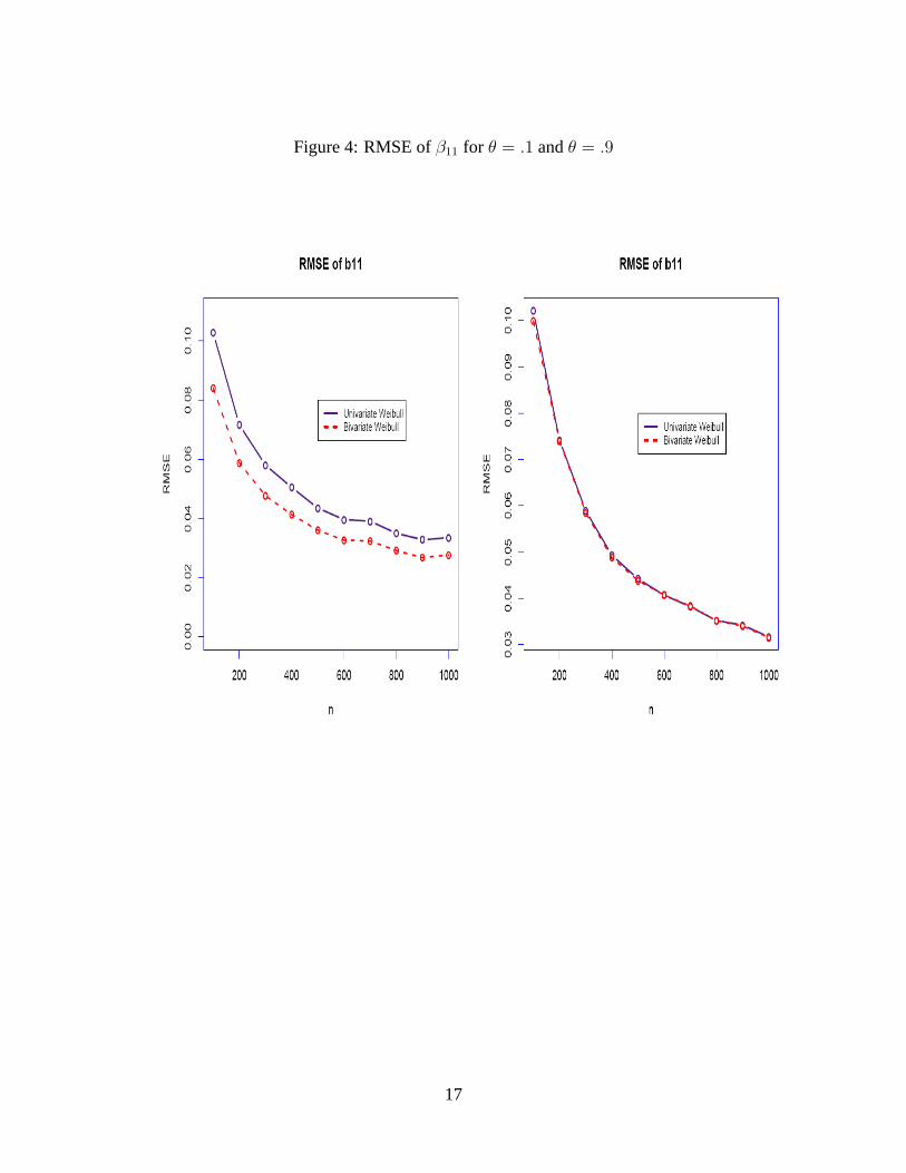
Figure 4: RMSE ofβ11 for θ = .1 andθ = .9

17

and the bivariate estimates are reduced by a large sample size, and the RMSE of the parameters

from the bivariate distribution remain smaller or equal than the RMSE of the parameters from the

univariate distribution.

The improvement in estimating the parameters of the bivariate distribution probably comes

from the better use of information regarding the association parameter. Indeed, only by estimat-

ing a bivariate distribution is it possible to know the strength of the interdependence between two

survival processes. This is a key finding, as the calculation of estimated probabilities, mean, and

median duration times, depends on the value of the association parameter. Moreover, as it was

mentioned previously in this paper, measures of association such as Pearson’s correlation coeffi-

cient, Kendall’s Tau, and Spearman’s Rho are also functions of this association parameter.

The derivation of the moments of the bivariate Weibull presented above is is not the focus

of this paper. However, Gumbel (1960) has presented the moments of a bivariate exponential,

whereas Johnson, Evans, and Green (1999), as well as Hays and Kachi (2008), have described

the moments of a particular bivariate Weibull. The real methodological challenge resides on the

estimation of the association parameter. This paper shows that the estimation of the association

parameter does not present significant problems if the appropriate algorithm and software are used.

The next section presents an application of these methods to a real data set.

7 Application: The joint survival time of leaders and foreign

ministers

In order to illustrate the use of a bivariate Weibull distribution, this paper analyzes the joint survival

of leaders and foreign ministers. During the last decade, the survival of leaders has been the

focus of extensive investigations (Bueno de Mesquita and Siverson 1995; Bueno de Mesquita,

Siverson, and Woller, 1992; Bueno de Mesquita et al. 2003; Chiozza and Goemans, 2003 and

2004; Goemans, 2000a and 2000b). However, not much research has been conducted on the

18

survival of other politicians in government, and even less on how the survival of one affects the

survival of the others (Berlinski, Dewan, and Myatt 2007; Dewan and Myatt 2005 and 2007).

In previous papers I contributed to this research agenda by developing and testing hypotheses

on the determinants of the tenure of foreign ministers. The evidence shows that although political

institutions have a significant impact on the tenure of foreign ministers, internal coalition dynamics

such as affinity and loyalty towards a leader, uncertainty, and time dependence are better predictors

of their political survival. Indeed, that investigation demonstrates that the survival of a leader has

a very significant impact on the survival of a foreign minister.

Nevertheless, it could be the case that the survival of a minister also has an impact on the

survival of a leader. Berlinski, Dewan, and Dowding (2007) and Dewan and Myatt (2005 and

2007) show that ministerial resignations in democratic, parliamentary systems do have a corrective

effect on the survival of a government. In addition, it is possible that external shocks could affect

the tenure of both leaders and ministers at the same time. This suggests that the survival times

of leaders and ministers are interdependent. Testing this hypothesis presents an ideal case for the

application of the methods developed in previous sections of this paper.

In order to test this hypothesis, this paper uses data on the tenure of leaders and foreign minis-

ters.6 The data set on foreign ministers constitutes the first systematic and entirely functional code

of the tenure of most foreign ministers for the last three centuries. The data set identifies 7,428

foreign ministers in 181 countries spanning the years 1696-2004, and includes the specific day,

month, and year in which 4,926 ministers took and left office. For the remaining 2,502 ministers,

only the years in which they took and left office were recorded. Ministers holding office up to

2004, as well as ministers from countries that disappeared, were recorded as right-censored.7 The

specific data used in estimation are for the ministers whose day, month, and year of taking and

6The data base on leaders is used by Bueno de Mesquita et al. (2003) and is publicly available athttp://www.nyu.edu/gsas/dept/politics/data/bdm2s2/Logic.htm.

7Up to this point there is no reliable information about the resignations of these foreign ministers. Thus, it isassumed that, if the ministers are not right-censored, they fail. Although ministers do resign from their positions, itis reasonable to assume that in general they try to stay in office for as long as possible. I believe it is better to testshypotheses with crude data than not to test them at all.

19

leaving office are known. These data include 4,420 foreign ministers in 156 countries from 1785

to 2000. In order to create this data set, all the ministers whose specific day, month, and year of

taking and leaving office are not known were dropped from the initial data set. In spite of this, the

sample used in estimation is still quite large.

In general, the data base would be organized as multiple-record data. In other words, there

would be a line of data for each year a leader and a minister hold office. This would capture

many time-varying covariates. However, this type of organization presents important challenges

for estimation. Therefore, this paper organizes the data as single-record data. There are two

dependent variables: the total survival time of a leader and the median survival time of ministers

that held office with that particular leader. For instance, if a leader lasted 9 years in office and had

3 ministers who held office for 2, 3, and 4 years respectively; the first dependent variable would be

equal to 9, whereas the second dependent variable would be equal to 3.8 Table 1 presents summary

statistics of the survival time of a leader, the median survival time of ministers, and the mean

failure of ministers by leader (Change in minister). This last variable is the main covariate used in

estimation. For instance, in the case of the leader that lasted 9 years in office, 3 ministers occupied

office as well. In those 9 years, 3 ministers failed. In this case, the variable would be equal to .3.

This means thatChange in ministercaptures the rate of minister change by year. The larger this

variable is, the more ministers have occupied office during the tenure of a particular leader.

Table 1: Summary statistics: yearsVariable N Mean Variance

Duration Leaders 1966 3.835 34.079Duration Median Ministers 1966 2.023 8.791

Change in minister 1966 .3583 .0955

Table 2 presents estimation results for the duration time of leaders and foreign ministers re-

spectively. The survival time of leaders depends on ministerial change, whereas the survival time

8There are other alternatives for data organization. Yet, given the current technology, this format is probably thebest way of analyzing the survival time of these two actors. Once the likelihood includes time-varying covariates,there will be no need to organize data according to arbitrary decisions.

20

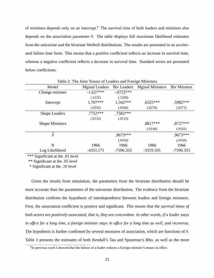
of ministers depends only on an intercept.9 The survival time of both leaders and ministers also

depends on the association parameterθ. The table displays full maximum likelihood estimates

from the univariate and the bivariate Weibull distributions. The results are presented in an acceler-

ated failure time form. This means that a positive coefficient reflects an increase in survival time,

whereas a negative coefficient reflects a decrease in survival time. Standard errors are presented

below coefficients.

Table 2: The Joint Tenure of Leaders and Foreign MinistersModel Mginal Leaders Biv Leaders Mginal Ministers Biv Minsters

Change minister -1.627*** -.6725***(.1222) (.1358)

Intercept 1.707*** 1.342*** .6325*** .5982***(.0535) (.0566) (.0270) (.0271)

Shape Leaders .7752*** .7582***(.0132) (.0133)

Shape Ministers .8817*** .8727***(.0144) (.0141)

θ .9673*** .9673***(.0550) (.0550)

N 1966 1966 1966 1966Log Likelihood -4355.171 -7596.353 -3319.105 -7596.353

*** Significant at the .01 level** Significant at the .05 level* Significant at the .10 level

Given the results from simulation, the parameters from the bivariate distribution should be

more accurate than the parameters of the univariate distribution. The evidence from the bivariate

distribution confirms the hypothesis of interdependence between leaders and foreign ministers.

First, the association coefficient is positive and significant.This means that the survival times of

both actors are positively associated, that is, they are concordant. In other words, if a leader stays

in office for a long time, a foreign minister stays in office for a long time as well, and viceversa.

The hypothesis is further confirmed by several measures of association, which are functions ofθ.

Table 3 presents the estimates of both Kendall’s Tau and Spearman’s Rho, as well as the more

9In previous work I showed that the failure of a leader reduces a foreign minister’s tenure in office.

21

familiar Pearson’s correlation coefficient.

Table 3: Measures of associationType of Association Association

Kendall .3099Spearman .4234Pearson .1802

This trend is also confirmed by the negative and significant coefficient forChange ministerin

the estimates from the bivariate distribution. In fact, if a foreign minister is removed, the survival

time of a leader is significantly reduced. Furthermore, the evidence shows that the survival time of

leaders and foreign ministers presents negative duration dependence, as the shape parameters are

significant and smaller than 1. This is indeed consistent with previous work on leaders (e.g. Bueno

de Mesquita et al. 2003) and ministers.

8 Conclusion

Motivated by the lack of methods to analyze the joint survival time of different subjects, this paper

proposes a specific method to estimate this type of interdependence. In the tradition of seemingly

unrelated regressions (SUR) or bivariate probit models, this paper assumes that the two different

survival processes are not independent. The interdependence between processes is modelled as part

of a bivariate distribution, which was derived from copula functions. Results from the simulation

experiment show that, for cases of strong interdependence between survival processes, the RMSE

of the parameters from the bivariate distribution are smaller than the RMSE of the parameters from

the univariate distribution. In addition, the parameters from the bivariate distribution are also more

efficient than the parameters from the univariate distributions. In cases of weak interdependence

between processes, the RMSE of the parameters from the bivariate and univariate distributions are

practically identical, and in some cases the RMSE of the parameters from the bivariate Weibull are

slightly smaller. Therefore,given the simplicity in estimating a bivariate Weibull, and regardless

22

of the degree of interdependence, it is recommended that the parameters from this distribution are

chosen over the parameters of a univariate Weibull.

This paper has taken a first step in the development of a consistent method to estimate joint

survival processes. Future research should concentrate on the development of a likelihood that

takes into account left-censoring, univariate censoring, and time-varying covariates. The exten-

sions to left-censoring and univariate censoring are not the most important issues regarding esti-

mation. However, given the organization of most data sets, it is extremely important to develop

the likelihood for time-varying covariates. The usual solution in the univariate world is to break

down the likelihood for a single subject into the intervals in which a covariate is kept constant

(Box-Steffensmeier and Jones 2004). Nonetheless, it is necessary to test whether this solution is

applicable to bivariate distributions. Moreover, since the observations with time-varying covariates

will not be independent, it is also imperative to know whether the standard errors need to be cor-

rected. This might require the calculation of complex residuals. When these extensions are carried

out, the methods presented here will have even more significant applications to political science

and other fields.

23

References

[1] Berlinski, Samuel, Torun Dewan, and Keith Dowding. 2007. The length of ministerial tenure

in the United Kingdom, 1945 to 1997.British Journal of Political Science37 (3): 245-262.

[2] Beck, Nathaniel, Jonathan N. Katz, and Richard Tucker. 1998. Taking time seriously: Time-

series cross-section analysis with a binary dependent variable.American Journal of Political

Science42 (4): 1260-1288.

[3] Boehmke, Frederick J., Daniel S. Morey, and Megan Shannon. 2006. Selection bias and

continuous-time duration models: Consequences and a proposed solution.American Journal

of Political Science50 (1): 192-207.

[4] Box-Steffensmeier, Janet M., and Bradford S. Jones. 2004.Event history modeling. A guide

for social scientists. New York: Cambridge University Press.

[5] Bueno de Mesquita, Bruce, and Randolph M. Siverson. 1995. War and the survival of political

leaders: A comparative study of regime types and political accountability.American Political

Science Review89 (4): 841-855.

[6] Bueno de Mesquita, Bruce, Randolph M. Siverson, and Gary Woller. 1992. War and the fate

of Regimes: A comparative analysis.American Political Science Review86 (3): 638-646.

[7] Bueno de Mesquita, Bruce, and Randolph M. Siverson. 1995. War and the survival of political

leaders: A comparative study of regime types and political accountability.American Political

Science Review89 (4): 841-855.

[8] Bueno de Mesquita, Bruce, Alastair Smith, Randolph M. Siverson, and James D. Morrow.

2003.The logic of political survival. Cambridge, MA: MIT Press.

[9] Chiozza, Giacomo, and H. E. Goemans. 2003. Peace through insecurity: Tenure and interna-

tional conflict.Journal of Conflict Resolution47 (4): 443-467.

24

[10] Chiozza, Giacomo, and H. E. Goemans. 2004. International conflict and the tenure of leaders:

Is war still ex post inefficient?American Journal of Political Science48 (3): 604-619.

[11] Devroye, Luc. 1986.Non-Uniform Random Variate Generation. New York, NY: Springer-

Verlag Press.

[12] Dewan, Torun, and David P. Myatt. 2005. The corrective effect of ministerial resignations.

American Journal of Political Science 49 (1): 46-56.

[13] Dewan, Torun, and David P. Myatt. 2007. Scandal, Protection and Recovery in the Cabinet.

American Political Science Review101 (1): 63-77.

[14] Diermeier, Daniel, and Randy T. Stevenson. 1999. Cabinet survival and competing risks.

American Journal of Political Science43 (4): 1051-1068.

[15] Goemans, H.E. 2000a. Fighting for survival: The fate of leaders and the duration of war.

Journal of Conflict Resolution44 (5): 555-579.

[16] Goemans, H.E. 2000b.War and punishment.Princeton, NJ: Princeton University Press.

[17] Gordon, Sanford C. 2002. Stochastic dependence in competing risks.American Journal of

Political Science46 (1): 200-217.

[18] Greene, William. 2003.Econometric analysis. New Jersey: Prentice Hall.

[19] Gumbel, E.J. 1960. Bivariate exponential distributions.Journal of the American Statistical

Association55 (292): 698-707.

[20] Hays, Jude C., and Aya Kachi. 2008.Government formation and dissolution in parliamentary

democracies: An empirical analysis using strategic survival models. Working Paper. Depart-

ment of Political Science, University of Illinois at Urbana-Champaign.

[21] Hougaard, Philip. 1986. A class of multivariate failure time distributions.Biometrika73 (3):

671-678.

25

[22] Johnson, Richard A., James W. Evans, and David W. Green. 1999.Some bivariate distri-

butions for modelling the strength properties of lumber. Research paper FPL-LR-575. United

States Department of Agriculture. Forest Service.

[23] Johnson, Mark E. 1986.Multivariate statistical simulation. New York: John Wiley and Sons.

[24] King, Gary, James E. Alt, Nancy Elizabeth Burns, and Michael Laver. 1990. A unified model

of cabinet dissolution in parliamentary democracies.American Journal of Political Science34

(3): 846-871.

[25] Lin, D.Y., and Zhiliang Ying. 1993. A simple nonparametric estimator of the bivariate sur-

vival function under univariate censoring.Biometrika80 (3): 573-581.

[26] Maddala, G.S. 1983.Limited dependent variables and qualitative variables in econometrics.

New York, NY: Cambridge University Press.

[27] Nelsen, Roger B. 2006.An introduction to copulas. New York, NY: Springer Science.

[28] Petersen, Trond. 1995. Models for Interdependent Event History Data: Specification and

Estimation.Sociological Methodology25: 317375.

[29] Spuler, Bertold, C.G. Allen, and Neil Saunders. 1977.Rulers and governments of the world.

Vols 2-3. London, UK: Bowker.

[30] Trivedi Pravin K., and David M. Zimmer. 2005. Copula modeling: An introduction for prac-

titioners.Foundations and Trends in Econometrics1 (1).

[31] Truhart, Peter. 1989.International directory of foreign ministers, 1589-1989. New York :

K.G. Saur.

[32] Tsai, Wei-Yann, Sue Leurgans, and John Crowley. 1986. Nonparametric estimation of a bi-

variate survival function in the presence of censoring.The Annals of Statistics14 (4): 1351-

1365.

26

[33] Tsai, Wei-Yann, and John Crowley. 1998. A note on nonparametric estimators of the bivariate

survival function under univariate censoring.Biometrika85 (3): 573-580.

[34] Van de Ven, W.P.M. and B.M.S. Van Pragg. 1981. The demand for deductibles in private

health insurance: A probit model with sample selection.Journal of Econometrics17 (2): 229-

252.

27