1

Copula-Based Pairs Trading Strategy

Wenjun Xie and Yuan Wu

Division of Banking and Finance, Nanyang Business School,

Nanyang Technological University, Singapore

ABSTRACT

Pairs trading is a technique that is widely used in the financial industry and its profitability

has been constantly documented for various markets under different time periods. The two

most commonly used methods in pairs trading are distance method and co-integration method.

In this research work, we propose an alternative approach for pairs trading using copula

technique. The proposed method can capture the dependency structure of co-movement

between the stocks and is more robust and accurate. Distance method and co-integration

method can be generalized as special cases of the proposed copula method under certain

dependency structures.

Keywords: pairs trading; copula; dependency structure; trading strategy

1. Introduction

“Pairs trading” is a well-known Wall Street investment strategy. It was first established by the

Wall Street quant Nunzio Tartaglia’s team in Morgan Stanley in 1980s. It was first

documented in literature by Gatev et al. (2006) where they tested the pairs trading strategy

using the daily data from 1962 to 2002 in the U.S equity market. It was documented that this

simple trading rule yields average annualized excess returns of up to 11% for self-financing

portfolios of pairs. Later, other people extended the analysis to various international markets

under different time periods and confirmed the profitability of this strategy. (Perlin, 2009;

Simone et al., 2010; Binh Do et al., 2010).

The main idea of pairs trading strategy is to find a pair of stocks which have strong co-

movement in prices in their history, and identify the relative over-valued and under-valued

positions between them in the following period. Such relative mispricing occurs if the spread

between the two stocks deviates from its equilibrium, and excess returns will be generated if

the pair is mean-reverting. The trading strategy is to long a stock that is under-valued and

short a stock that is over-valued at the same time, and close the positions when they return to

fair values.

There are two most commonly used methods in pairs trading. The first is called distance

method. The main idea of this method is to use the distance between the standardized prices

of two stocks as the criteria to select pairs and form trading opportunities (Gatev et al., 2006;

Perlin, 2009; Simone et al., 2010; Binh Do et al., 2010). Another method is called co-

integration method. It uses the idea of co-integrated pairs proposed by Nobel laureate Clive

Granger (1987). If two stocks are co-integrated with each other, the difference in their returns

should perform mean-reverting property. Then long/short positions are constructed when the

2

difference is relatively large and closed when the difference reverts to its mean level (Lin et

al., 2006; Galenko et al., 2012).

Despite the success of this trading strategy documented in the literature, recent research

conducted by Binh Do et al. (2010) confirmed the downward trend in profitability of pairs

trading strategy. They proposed alternative methods such as choosing pairs within confined

industry to increase the profitability.

Both distance method and co-integration method involves the idea of spread. They use spread

either between standardized prices or returns to capture the idea of mispricing. Equal spreads

are assumed to have same levels of mispricing regardless of the stock prices and returns. If

the data is jointly normally distributed, then linear correlation completely describes

dependency, and the distribution of spread is stationary under different prices and returns. On

the other hand, the dependence between two variables has both linear and non-linear

components, and it has many other forms of expressions rather than simple linear correlation

coefficient, e.g. tail dependence. It is widely accepted that the financial data are rarely

normally distributed in reality, and therefore correlation cannot completely describe the

dependency structure (Kat, 2003; Crook and Moreira, 2011).

In this research work, a new algorithm for pairs trading using copula technique is proposed,

and it will capture the dependency structure of the stocks. Liew and Wu (2013) documented

several empirical evidences of extra profits using copula technique in pairs trading. The

purpose of this research is to set up the theoretical foundation of copula-based pairs trading

strategy and make comparison with traditional methods. We are not claiming that it is

superior to distance method or co-integration method, but it provides an alternative way to

looking at pairs trading.

The idea of copula arose as early as 19th century in the context of discussions regarding non-

normality in multivariate cases. Sklar (1959) set the foundation of copula method which links

the joint distribution of two variables to their separate margins. The advantage of copula

method is that it describes the structure of dependence between several variables, and thus is

more robust and accurate.

As mentioned earlier, linear correlation can fully explain the dependency structure if the two

stocks follow joint normal distribution. In this research, it is shown that distance method can

be generalized as a special case of copula method if the data do follow joint normal

distribution. It is also shown that the co-integration method will generate the same trading

opportunities as copula method under certain restrictions. In reality, the data structure is often

complicated and no one knows the true marginal distributions and joint relation. Copula

method has the advantage of estimating optimal marginal distributions and optimal copula

separately, and thus has the optimal estimation of the joint distribution between two stocks,

resulting in more trading opportunities. Several examples will be given to illustrate these

points. Note therefore that, we only focus on the trading strategy at the current stage and

assume that the pairs are already selected out.

The rest of the paper is organized as follows: Section 2 describes the traditional methods and

introduces the new trading algorithm using copula technique. Section 3 generalizes current

methods as special cases of copula methods under certain conditions and real examples are

given. Section 4 concludes the paper.

3

2. Trading algorithm using copula method

2.1 Two commonly used methods in pairs trading

Assuming the pair, stock X and stock Y, is already picked out as the candidate for pairs

trading, either by distance method or co-integration method. Under the general framework of

pairs trading, the prices of the stocks from the selected pair are assumed to move together

over time. In other words, under the arbitrage pricing model (APT), the two stocks should

have exactly same risk factors exposures, and the expected returns in a given time duration

are the same.

Now, we define and

to be the prices of stock X and stock Y at time t respectively (

and at time 0), and

and to be the cumulative returns of the stock X and stock Y at

time t .Then

.

By taking logarithm at both sides, we obtain that

(

) ( )

(

) ( ).

According to the APT model, the expected return of stock X should equal to the expected

return of stock Y at time t as long as the stock X and stock Y share the same risk factors

exposures, i.e. ( ) (

) . Moreover, and

can be expressed in the

following form:

(

)

(

)

.

and

represent the error terms which make the returns of stock X and stock Y deviate

from the expected returns, and ( ) (

) .

Two commonly used methods in pairs trading are distance method and co-integration method.

For the distance method, it uses the spread between the standardized prices of the two stocks

as the measurement of degree of mispricing. For the co-integration method, it uses the spread

between the returns of the two stocks as the measurement. The idea of spread captures how

close the two stocks are. If the two stocks follow joint normal distribution, it can be easily

proved that the distribution of the spread in both distance method and co-integration method

are robust, and the spread itself fully captures the dependency structure of the two stocks.

However, in reality, the true distribution of the error terms and

are unknown, and the

dependency structure of the error terms and the expected return is also unobservable,

which makes the assumption of joint normal distribution invalid.

The disadvantages of the current measurements of degree of mispricing under distance

method or co-integration method are similar and can be illustrated from two aspects, although

our illustration is centered on co-integration method here. For example, if the trading strategy

is to construct long/short positions when the spread between the returns of two stocks,

4

, is larger than or smaller than and close the positions when the spread return

to 0. The following two situations may happen:

Situation 1

Although the spread between the returns of two stocks has reached , however, conditioning

on the level and

, the variance of the spread tends to be larger than the mean sample

variance. Thus, a potential scenario is that the spread will continue to grow larger.

Consequently, the long/short position entering at spread equal to may reach the pre-

determined stop-loss position and it results in a loss of capital. Another scenario is that it may

require longer time to revert to the 0 spread position. Neither of the scenarios is preferred by

investors.

Situation 2

Next, we consider a time point which the spread is still less than , however, conditioning on

the return level and

, the spread tends to have smaller variance than the mean sample

variance, so it may already be a good opportunity to trade. Considering the criteria that we

only trade when the spread is larger than or smaller than , this trading opportunity is

missed.

Two simulated series of stock prices are used to illustrate the above two situations. Figure 1(a)

shows the movement of the two simulated series of stock prices. The vertical line divides the

whole sample into formation period and trading period. Dickey-Fuller test has been used to

confirm that they are co-integrated pairs. Figure 1(b) shows the spread of the return between

them. It is simulated with the property that the variance of the spread is higher when the stock

prices are at high level, which is , and the variance of the spread is lower when the stock

prices are at low level, which is . The bounds refer to the 1.65 level lines, where is the

variance of the spread during formation period. It is easily known that . We use

this value 1.65 as the threshold value . Consequently, at high price levels, after reaching

, the spread is going to grow larger and results in unfavorable situation. This is because the

true at high price level is larger than , so it is optimal to trade when the spread reach

1.65 instead of 1.65 . Again, at low price levels, some opportunities are missed by co-

integration method since it is optimal to trade when the spread reach 1.65 instead of

1.65 .

Through this example, it can be said that traditional pairs trading methods are not optimal if

there are different dependency pattern conditioning on different price levels. It is common

that the real data does not have such apparent patterns of variances at different price levels,

but different patterns of spreads do exist for different price levels. This example is used as a

magnifying version of the potential real situation. The distance method may produce the same

situations as above.

2.2 A new measurement of degree of mispricing

Considering the situations discussed above, measurements of mispricing used in traditional

methods (distance method and co-integration method) are robust only under the validity of

joint normal distribution assumption. A new measurement of mispricing is desirable if it is

able to remove the restrictions required by traditional methods, and should also have the

following properties:

5

Comparability – For a given time point, the numerical value of this measurement can reflect

the degree of mispricing. By comparing the values of this measurement in two realizations, it

can be decided which realization is more mispriced.

Consistency - This measurement has to be consistent and comparable over different time

periods and return levels. This means that two situations are of same degree of mispricing if

and only if their measurements are of the same numerical values no matter what the time

period and expected return levels are.

To satisfy the above properties, a new measurement of the degree of mispricing is proposed.

Definition Given time t, the returns of the two stocks are

and

. Define

(

), the conditional probability of stock X’s return smaller than the current

realization given the stock Y’s return equal to current realization

as the Mispricing

Index of X given Y, denoted as . is defined in the same way.

Theorem 1 Assuming and are two possible scenarios of the stock prices at time t.

and

in scenario E while

and

in scenario . ( )

( ) .

,

,

,

and

. > if and

only if

.

Proof. (

)

(

)

(

)

(( ) (

))

)

(

)

(

( ) (

)

)

(

)

Although the detailed numerical values of and

are not observed, the difference,

however, is captured by the difference of returns. It can be seen that is a monotonic

increasing function of

given that

. This suggests that a higher value of

indicates a higher degree of mispricing, and thus satisfies the comparability property. #

The consistency of this new measurement can be understood intuitively. Although the idea of

spread is not used directly in , it still explores the similar idea. The conditional

probability of return of stock X smaller than the current realization given the return of stock Y

fixed can be seen as the conditional probability that the spread smaller than the current

realization given the return of stock Y fixed. As discussed above, the traditional methods

ignore the non-linear correlation between the spread and the return levels. For the new

measurement , it is able to obtain the conditional distribution of the spread given each

level of returns. indicates the likelihood that the spread is smaller than the current

realization when given the information. Since the likelihood is comparable across different

time periods and return levels, it can be concluded that is consistent.

In the traditional methods, the mean-reverting property of the spread is assumed. For the new

measurement, though we condition the spread on the return levels, it is assumed that it only

affects the shape of the distribution, and will still perform mean-reverting property.

6

Theorem 2 If the current realizations of returns of stock X and stock Y equal to the expected

return , then

Proof. (

)

(

)

(

)

(

)

( (

) )

( (

) )

(

)

(

)

(

)

( )

=0.5 #

This suggests that when the error terms of the returns of the two stocks equal 0, should

be equal to 0.5, which means that under fair prices, is 0.5. Similarly, it can be proved

that under fair prices, is also 0.5.

Corollary If , then stock X is overpriced relative to stock Y.

If , then stock X is fairly priced relative to stock Y.

If , then stock X is underpriced relative to stock Y.

It has been discussed that the new measurement has the property of comparability and

consistency. Under fair prices, the is 0.5, and this means that stock X is fairly priced

relative to stock Y when . However, this does not only apply to the situation that

stock Y is really fairly priced. In the real market, we never observe what the true expected

return is. However, due to consistency, we can conclude that stock X is fairly priced relative

to stock Y if . When , stock X is overpriced relative to stock Y, and

when , the stock X is underpriced than stock Y.

2.3 Mispricing index under copula framework

The procedure to obtain or using copula technique is provided below. The

marginal distributions of the returns of stock X and Y are assumed to be and , while joint

distribution is

Theorem 3 (Sklar’s Theorem) If )(F is a n-dimensional cumulative distribution function for

the random variables with continuous margins nFF ,...,1 , then there exists a

copula function C, such that

))(),...,((),...,( 111 nnn xFxFCxxF .

If the margins are continuous, then C is unique. If any distribution is discrete, then C is

uniquely defined on the support of the joint distribution.

7

Let ( ) and (

). According to Sklar’s theorem, we can always identify a

unique copula C which satisfies the following equation:

( ) ( ) ( ) (

) .

Theorem 4 Given current realization of returns of stock X and stock Y ( ), we have:

( )

( )

.

Proof. Given ( ), the mispricing index of X given Y can be calculated as:

( ) ( ) (

) ( ) (

) .

Let ( ) and (

), then:

( ) ( )

.

Similarly, we obtain that

( ) ( )

. #

2.4 Copula-based pairs trading algorithm

Similar to the distance method and co-integration method, the trading strategy using copula

technique still consists of two periods, which are formation period and trading period. Below

is the trading algorithm assuming pair X and Y is already selected.

Step 1. Calculate daily returns for each stock during formation period. Estimate the marginal

distributions of returns of stock X and stock Y, which are and separately.

Step 2. After obtaining the marginal distributions, estimate the copula described by Sklar’s

theorem to link the joint distribution with margins and , denoted as C.

Step 3. During trading period, daily closing prices and

are used to calculate the daily

returns (

). Therefore, and can be calculated for every day in the trading

period by using estimated copula C.

Step 4. Construct short position in stock X and long position in stock Y on the day that

and if no positions in X or Y is held. Construct long position in stock

X and short position in stock Y on the day that and if no positions in

X and Y is held. The market value of short positions should always equal to the market value

of long positions at the start. All positions are closed if reaches or reaches ,

where all pre-determined threshold values are.

3. Generalization of traditional methods

It has been explained that the traditional methods use the idea of spread, and are more robust

when linear correlation captures the whole dependency structure of two stocks. In this section,

we show that the traditional methods can be generalized into special cases of copula method

under certain assumptions about the marginal distributions and the joint relation.

8

3.1 A special Case: Distance Method

Under assumptions of normal marginal distributions of the stock prices and normal copula of

the joint relation between the stock returns, it can be shown that the distance method will

generate the same result as the copula-based trading strategy.

The distance method uses standardized prices in the calculation. Denote and

as the

standardized prices of stock X and stock Y. Then they follow standard normal distributions

with mean 0 and variance 1 if the marginal distributions of stock prices are assumed to be

normal. Denote as the spread between them, and thus

. Denote as the

linear correlation between the two stocks, then:

( ) (

) ( )

( ) (

)

( ) (

) (

)

.

This shows that follows normal distribution with mean 0 and variance under the

distance method framework. It is stationary, and neither the mean nor the variance changes

with the time t or the price levels and

.

Now, let us look at the copula method under assumptions of normal marginal distributions of

the stock prices and normal copula linking them.

Theorem 5 Let X and Y be continuous random variables with copula CXY. If functions and

are strictly increasing on RanX and RanY, respectively, then ( ) ( ) . Thus CXY is

invariant under strictly increasing transformations of X and Y.

Proof of this theorem can be found in Nelson (2006).

Since (

) ( ) and

( ) (

) , and

are all strictly

increasing transformations of and

. Therefore,

.

It is assumed that the copula linking and

is normal, so that the copula linking and

is also normal. Combing with the information that

and have normal marginal

distributions, it can be proved that and

are joint normally distributed with being the

linear correlation coefficient between X and Y.

Consequently, the mispricing index can be calculated in the following manner, which

is related to the distribution of

.

(

)

(

)

(

)

(

)

9

Theorem 6. If random variables X and Y follow standard normal distributions, and are jointly

distributed with linear correlation coefficient , then X|Y=y follows normal distribution with

mean and variance .

Proof. Assuming ( ) is the density function of the random variable X|Y=y. A~B means A

is linearly proportional to B.

( ) ( )

( )

( )

√ (

( ))

( ) ( ) (

( )),

( ) ( ( )

( ))

Thus, X|Y=y follows normal distribution with mean and variance . #

Since and

are jointly normally distributed, and

should also be jointly

normally distributed. Then the conditional distribution of given

should

follow normal distribution with mean and variance . Then

(

)

( )

(

) .

This shows that

|

follows normal distribution with mean ( )

and variance . In other words, the spread between two standardized prices

conditional on

is assumed to follow normal distribution with mean ( )

and variance .

For pairs trading, the linear correlation coefficient should be close to 1, which means

(

) approaches 0. Moreover, since the variance of

is ,

which is independent of the price levels, it can be concluded that the distribution of the spread

is robust across different price levels. Therefore, distance method can capture the optimal

trading opportunities the same as copula method under assumptions of normal marginal

distributions and normal copula. However, if these assumptions do not hold for the real data,

distance method may not be optimal.

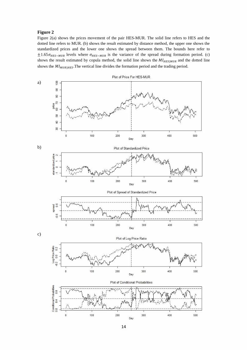
Two real data examples are used to illustrate the above analysis. The first one shown in

Figure 2 uses the pair HES (Hess Corporation) and MUR (Murphy Oil Corporation). It is one

of the stock pairs studied in Chiu et al. (2011), and is listed on PairsLog.com as a basic

materials/oil pair. Daily stock prices from January 2010 to December 2011 are downloaded

from Yahoo Finance. The first year data is used as the formation period and the second year

data is used as the trading period. The movement of the stock prices is shown in Figure 2(a),

and we can see that they have a strong co-movement. The standardized prices and the spread

between them are shown in Figure 2(b), the two bounds represent the 1.65 levels

corresponding to 95%/5% probability level in the copula method shown in Figure 2(c) while

is the variance of the spread during formation period. In Figure 2(c), normal

distribution is chosen to estimate the marginal distributions of stock prices and normal copula

10

is chosen to best fit the joint relation between stocks. By doing so, the result calculated from

copula method matches exactly the result from distance method. The line in Figure 2(b) has

the same shape as the line in Figure 2(c).

Another example uses the pair BKD (Brookdale Senior Living) and ESC (Emeritus), which is

also listed in PairsLog.com. The time period is from December 2009 to November 2012. The

first 2 years data are used to form the formation period while the rest are used to form the

trading period. Price co-movement is shown in Figure 3(a). The results calculated from

distance method and copula method are shown in Figure 3(b) and (c) respectively. Here, the

marginal distributions are best fitted by generalized extreme value distributions, and the

estimated copula is gumbel copula. The bounds here have the same meaning as the previous

sample.

Different from the previous sample, it is found that the two methods give different results. It

is found that the copula method captures more trading opportunities that are overlooked by

the distance method. This is consistent with the analysis above. Distance method only

produces same result as the copula method when the data structure is indeed estimated by

normal margins and normal copula. When the data structure is best fitted by other marginal

distributions and copulas, the copula method gives more trading opportunities.

From the above analysis, it can be seen that the distance method is a special case of the

proposed copula-based trading strategy under certain assumptions. If the real data structure is

indeed captured by normal marginal distributions and normal copula, the result generated by

distance method is the same as the copula method. However, in the real data structure, the

normal assumptions are not always valid. Copula method can capture the structure of

dependence rather a single measurement of spread, and is more robust and consistent.

3.2 A special case: co-integration Method

As mentioned earlier, the co-integration method assumes that same spread across different

return levels has the same degree of mispricing. It is argued that the detailed dependency

structure of error terms and expected return levels are complex and cannot be generalized to

one fixed distribution across all price levels. Thus, the co-integration method may not be

optimal under some real data structure.

From mathematical point of view, if the data structure has the intrinsic property

( ) ( |

)

if

for any

,

in other words,

if

,

,

then the co-integration method will generate the same trading opportunity as the copula

method if the threshold values are chosen carefully. It is hard to tell the assumptions of the

marginal distributions and joint relation exactly for co-integration method, however, it can be

seen that the co-integration method do put on more restriction in the data structure compared

11

to the copula method. This kind of restriction sometimes overlooks the non-linear correlation

between stock prices, and thus misses some trading opportunities.

It is difficult to give examples to show that co-integration method produces the same result as

the copula method under some assumptions like the first example in the previous section. The

reason is that the restriction described by co-integration method is hard to be satisfied using

several simple assumptions about the margins and copula. However, an example on the

difference of copula method and co-integration method can still be given. BKD-ESC pair is

used to illustrate the idea here again. The same time period as the previous section is used.

The results calculated from the co-integration method and the copula method are shown in

Figure 4(b) and (c). It is obvious that copula method captures more trading opportunities. The

reason for this is that the data structure has strong tail dependence, and it shows different

patterns of correlation at different price levels. BKD tends to be largely higher than ESC at

high price levels while it is not that obvious at low price levels. However, co-integration

method does not capture this characteristic, and thus overlooks potential trading opportunities.

4. Conclusions

In this research work, an algorithm for pairs trading using copula technique is proposed. On

the one hand, traditional methods such as distance and co-integration methods use the idea of

spread in their trading strategy. When the two stocks follow joint normal distributions, the

linear correlation can capture the whole dependency information and the distribution of

spread is robust under different price levels. On the other hand, copula method captures the

dependency structure of the two stocks which is more robust and accurate. Under certain

assumptions, traditional methods can be generalized as special cases of copula method.

Overall, we provide an alternative way to look at pairs trading. The future research could

focus on testing the profitability of the copula method by implementing the real data and

incorporate this method in pairs selection process.

12

References

Chiu, J., Lukman, D. W., Modarresi, K., and Velayutham, A. S. (2011) High-frequency

Trading. Standford, California, U.S.: Stanford University.

Crook, J., and Moreia, F. (2011) Checking for asymmetric default dependence in a credit card

portfolio: A copula approach. Journal of Empirical Finance 18(4): 728-742.

Engle, R. F. and Granger, C. W. J. (1987). Co-integration and error-correction:

Representation, estimation and testing. Econometrica 55 (2): 251–276.

Do, B., and Faff, R. (2010) Does Simple Pairs Trading Still Work? Financial Analysts

Journal 66(4): 83-95.

Galenko, A., Popova, E., and Popova, I. (2012) Trading in the Presence of Co-integration.

The Journal of Alternative Investments 15(1): 85-97.

Gatev, E., Goetzmann, W. N., and Rouwenhorst, K. G. (2006) Pairs Trading: Performance of

a Relative-Value Arbitrage Rule. The Review of Financial Studies 19(3):797-827.

Kat, H. M. (2003) The Dangers of Using Correlation to Measure Dependence. The Journal of

Alternative Investments 6(2): 54-58.

Liew, R. Q. and Wu, Y. (2013). Pairs trading: A copula approach. Journal of Derivatives and

Hedge Funds, Vol 19(1), pp12-30.

Lin, Y.-X., MaCrae, M., and Gulati, C. (2006) Loss Protection in Pairs Trading Through

Minimum Profit Bounds: A Co-integration Approach. Journal of Applied Mathematics and

Decision Sciences 2006: 1-14.

Nelson, R. B. (2006) An Introduction to Copulas (2nd

Ed.). New York: Springer.

Perlin, M. S. (2009) Evaluation of Pairs-Trading Strategy at the Brazilian Financial Market.

Journal of Derivatives& Hedge Funds 15(2): 122-136.

Simone, B. and Alessandro, G. (2010) A Pairs Trading Strategy Applied to the European

Banking Sector. Lecture “Asset Allocation and Performance Measurement”, University of

Zurich, spring 2010.

Sklar, A. (1959) Functions de répartition a n dimensions et leurs marges. Publications de

l’Institut de Statistique de L’Universite de Paris 8:229-231.

13

Figure 1

Figure 1(a) shows the prices movement of two simulated stocks. (b) shows the spread between their

returns. The solid line refers to stock X and the dotted line refers to stock Y. The simulation is designed

to satisfy that the variance of the spread is larger when the stock prices are higher and lower when the

stock prices are lower. The vertical line divides the formation period and the trading period.

a)

b)

14

Figure 2

Figure 2(a) shows the prices movement of the pair HES-MUR. The solid line refers to HES and the

dotted line refers to MUR. (b) shows the result estimated by distance method, the upper one shows the

standardized prices and the lower one shows the spread between them. The bounds here refer to

1.65 levels where is the variance of the spread during formation period. (c)

shows the result estimated by copula method, the solid line shows the and the dotted line

shows the .The vertical line divides the formation period and the trading period.

a)

b)

c)

15

Figure 3

Figure 3(a) shows the prices movement of the pair BKD-ESC. The solid line refers to BKD and the

dotted line refers to ESC. (b) shows the result estimated by distance method, the upper one shows the

standardized prices and the lower one shows the spread between them. The bounds here refer to

1.65 levels where is the variance of the spread during formation period. (c) shows

the result estimated by copula method, the solid line shows the and the dotted line shows the

.The vertical line divides the formation period and the trading period.

a)

b)

c)

16

Figure 4

Figure 4(a) shows the prices movement of the pair BKD-ESC. The solid line refers to BKD and the

dotted line refers to ESC. (b) shows the result estimated by co-integration method, the upper one shows

the log price returns and the lower one shows the spread between them. The bounds here refer to

1.65 levels where is the variance of the spread during formation period. (c) shows

the result estimated by copula method, the solid line shows the and the dotted line shows the

.The vertical line divides the formation period and the trading period.

a)

b)

c)