Convolutional Neural Network Hyper-Parameters Optimization ...€¦ · applications, Convolutional...

(IJACSA) International Journal of Advanced Computer Science and Applications,

Vol. 9, No. 10, 2018

252 | P a g e

www.ijacsa.thesai.org

Convolutional Neural Network Hyper-Parameters

Optimization based on Genetic Algorithms

Sehla Loussaief1, Afef Abdelkrim

2

Laboratory of Research in Automatic (LA.R.A)

National Engineering School of Tunis (ENIT), University of Tunis El Manar

National Engineering School of Carthage (ENICarthage), University of Carthage

Tunis, Tunisia

Abstract—In machine learning for computer vision based

applications, Convolutional Neural Network (CNN) is the most

widely used technique for image classification. Despite these deep

neural networks efficiency, choosing their optimal architecture

for a given task remains an open problem. In fact, CNNs

performance depends on many hyper-parameters namely CNN

depth, convolutional layer number, filters number and their

respective sizes. Many CNN structures have been manually

designed by researchers and then evaluated to verify their

efficiency. In this paper, our contribution is to propose an

innovative approach, labeled Enhanced Elite CNN Model

Propagation (Enhanced E-CNN-MP), to automatically learn the

optimal structure of a CNN. To traverse the large search space

of candidate solutions our approach is based on Genetic

Algorithms (GA). These meta-heuristic algorithms are well-

known for non-deterministic problem resolution. Simulations

demonstrate the ability of the designed approach to compute

optimal CNN hyper-parameters in a given classification task.

Classification accuracy of the designed CNN based on Enhanced

E-CNN-MP method, exceed that of public CNN even with the use

of the Transfer Learning technique. Our contribution advances

the current state by offering to scientists, regardless of their field

of research, the ability of designing optimal CNNs for any

particular classification problem.

Keywords—Machine learning; computer vision; image

classification; convolutional neural network; CNN hyper

parameters; enhanced E-CNN-MP; genetic algorithms; learning

accuracy

I. INTRODUCTION

Image classification is an important task in computer vision involving a large area of applications such as object detection, localization and image segmentation [1-3]. The most adopted methods for image classification are based on deep neural network and especially Convolutional Neural Networks (CNN). These deep networks have demonstrated impressive and sometimes human-competitive results [4,5]. CNN deep architecture can be divided in two main parts [6]. The first part, based on convolutional layers CNN, offers the ability of features extraction and input image encoding. Whereas, the second one is a fully connected neural network classifier which role is to generate a prediction model for the classification task. A CNN model is described by many hyper-parameters specifically convolutional layers number, filters number and their respective sizes, etc.

Many researchers proposed different CNN models such as AlexNet, Znet, etc. To improve the network accuracy some of them choose to increase the depth of the network [7]. Others propose new internal configurations [8]. Although, these state-of-the-art CNNs have been shown to be efficient, many of them were manually designed.

During our research, we note that a miss configured values of CNN hyper-parameters namely the network depth, the number of filters and their respective sizes dramatically affect the performance of the classifier. In addition, manually, enumerating all the use cases and selecting optimal values for these hyper-parameters is almost impossible even with a fixed number of convolutional layers. Through contributions held in this paper we propose an innovative approach, labeled Enhanced Elite CNN Model propagation (Enhanced E-CNN MP), to automatically learn optimal CNN hyper-parameters values leading to a best CNN structure for a particular classification problem. Our approach is based on Genetic Algorithms (GA) known to be meta heuristic methods for non-deterministic problem resolution. Each CNN candidate solution structure, is encoded as an individual (chromosome). To search for the best fit individual, the proposed method is based on “The elite propagation” through the whole GA process.

The designed Enhanced E-CNN MP approach is an innovative approach. Our contribution will allow scientists to design their own CNN based prediction model suitable for their particular image classification problem.

This paper is organized as follows. Section II provides an overview of Convolutional Neural Network. In section III, the Genetic Algorithms paradigm is exposed. Problem statement is presented through section IV. Section V introduces related work. Section VI illustrates the designed Elite CNN Model Propagation (E-CNN-MP) approach based on GAs for CNN hyper parameters optimization. E-CNN-MP simulations and results are presented in section VII. Through section VIII, an Enhanced E-CNN-MP version is proposed. The last section includes our concluding remarks.

II. DEEP LEARNING BASED ON CONVOLUTIONAL NEURAL

NETWORK

A neural network is a mathematical model with a design inspired from biological neurons. This network architecture is divided in layers. Each layer is a set of neurons. The first layer of a neural network is the input layer into which we inject the


Vol. 9, No. 10, 2018

253 | P a g e


data to be analyzed. The last layer is the output layer. In a classification problem, it returns a number of classes. Layers on the middle are the hidden layers of the neural network.

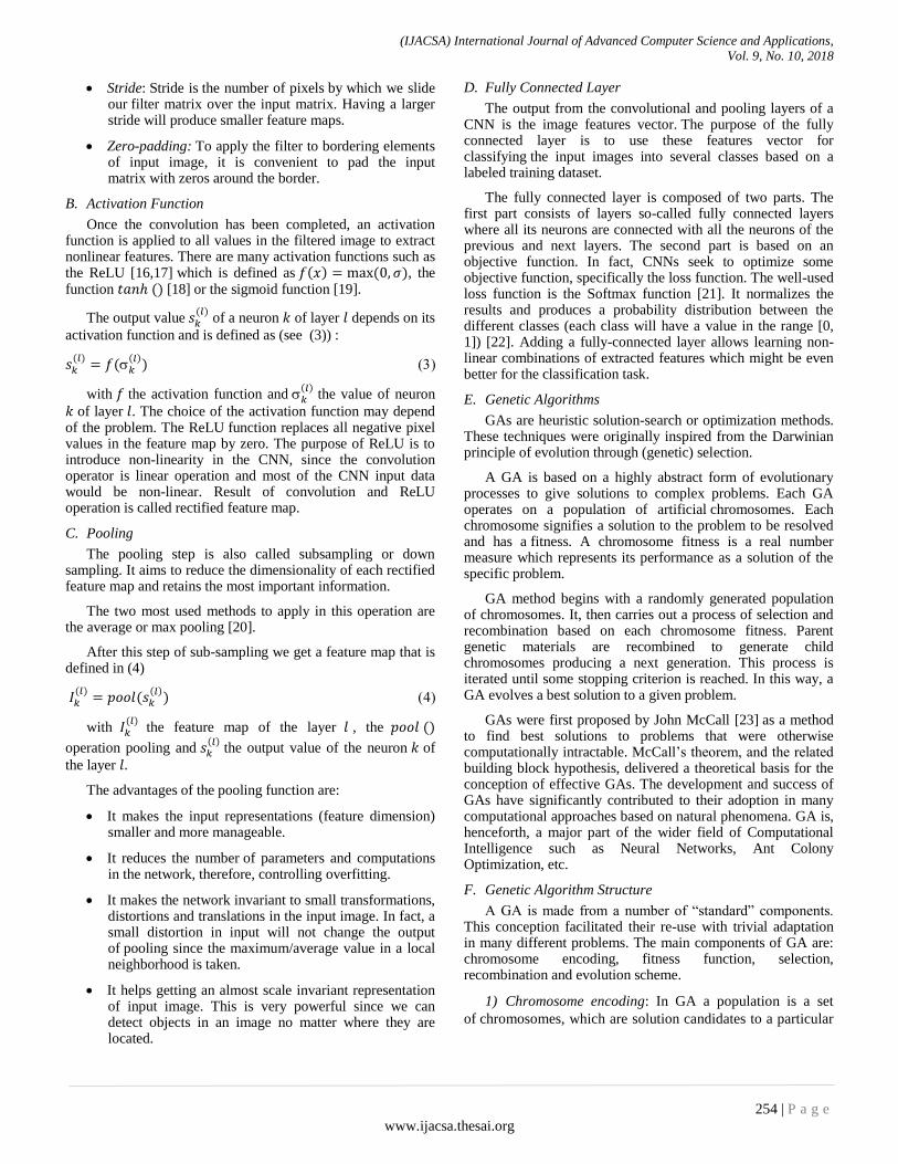
As shown in Fig.1, in a neural network, a single neuron has several inputs. Each input connection is characterized by a weight . On the activation of the artificial neuron, it computes its state , by summing all the inputs multiplied by their corresponding connection weights. To ensure that the neuron will be activated even when all entries are none, an extra input, called bias , is added. This extra input is always equal to 1 and has its own weight connection.

To normalize its result (normally between 0-1), the neuron passes it through its activation function [9].

Fig. 1. Neuron Parameters.

CNNs are category of deep neural networks used especially in computer vision area such as image classification [10,11]. The very first CNN was LeNet in 1990 (LeCun et al. 1995). It was the innovative work by Yann LeCun and the result of many successful iterations since the year 1988. This pioneering CNN facilitated propel the field of deep learning. At that time the LeNet architecture was used mainly for character recognition application.

There have been numerous new CNN architectures developed in the recent years. These architectures are improvements over the LeNet using its main concepts. Among these models we quote:

AlexNet (2012): In 2012, Alex Krizhevsky (and others) released AlexNet. It was a deeper and much wider version of the LeNet that won, by a large margin, the difficult ImageNet Large Scale Visual Recognition Challenge (ILSVRC) in 2012.

ZF Net (2013): The ILSVRC 2013 winner was a Convolutional Network from Matthew Zeiler and Rob Fergus. It became known as the ZFNet. It was an improvement on AlexNet by tweaking the architecture hyper-parameters.

GoogLeNet (2014): The ILSVRC 2014 winner was a Convolutional Network from Szegedy (and others) from Google. Its main contribution was the development of an inception module that dramatically reduced the number of parameters in the network (4M, compared to AlexNet with 60M) [12].

VGGNet (2014): The runner-up in ILSVRC 2014 was the network that became known as the VGGNet. Its main contribution was in showing that the depth of the network (number of layers) is a critical component for good performance.

ResNets (2015): Residual Network developed by Kaiming He (and others) was the winner of ILSVRC 2015.

DenseNet (August 2016): Recently published by Gao Huang (and others). The Densely Connected Convolutional Network has each layer directly connected to every other layer in a feed-forward fashion. The DenseNet has been shown to obtain significant improvements over previous state-of-the-art architectures on five highly competitive object recognition benchmark tasks.

There are four main operations which are the basic building blocks of every CNN [13,14].

1) Convolution

2) Activation function (ReLU)

3) Pooling or Sub Sampling

4) Classification (Fully Connected Layer)

A. Convolution

Convolutional layer derives its name from the convolution operator. The aim of this layer is image features extraction. Convolution conserves the spatial relationship between pixels by learning image features using small squares of input data. Each convolution layer uses various filters to features detection and extraction such as Edge Detection, Sharpen, Blur, etc. These filters are also called „kernels‟ or „feature detectors‟. After sliding the filter over the image we get a matrix known as the feature map [15].

In the first convolution layer, the convolution is between the input image and its filters. Filter values are the neuron weights (see (1)).

In deep layers of the network, the resulting image of

convolutions is the sum of convolutions, with the number of outputs of layer (see (2)).

(1)

∑

With

the value of the neuron of the layer ,

the

input vector of the neuron ,

the weight vector and

the bias.

In practice, a CNN learns the values of these filters on its own during the training process. Parameters such as number of filters, filter size and network architecture are specified by the scientific before launching the training process. The more number of filters we have, the more image features get extracted and the better the network becomes at features extraction and image classification.

The size of the feature map is controlled by three parameters which are:

Depth: Depth corresponds to the number of filters used for the convolution operation.


Vol. 9, No. 10, 2018

254 | P a g e


Stride: Stride is the number of pixels by which we slide our filter matrix over the input matrix. Having a larger stride will produce smaller feature maps.

Zero-padding: To apply the filter to bordering elements of input image, it is convenient to pad the input matrix with zeros around the border.

B. Activation Function

Once the convolution has been completed, an activation function is applied to all values in the filtered image to extract nonlinear features. There are many activation functions such as the ReLU [16,17]

which is defined as , the

function [18] or the sigmoid function [19].

The output value

of a neuron of layer depends on its

activation function and is defined as (see (3)) :

with the activation function and

the value of neuron

of layer . The choice of the activation function may depend of the problem. The ReLU function replaces all negative pixel values in the feature map by zero. The purpose of ReLU is to introduce non-linearity in the CNN, since the convolution operator is linear operation and most of the CNN input data would be non-linear. Result of convolution and ReLU operation is called rectified feature map.

C. Pooling

The pooling step is also called subsampling or down sampling. It aims to reduce the dimensionality of each rectified feature map and retains the most important information.

The two most used methods to apply in this operation are the average or max pooling [20].

After this step of sub-sampling we get a feature map that is defined in (4)

with

the feature map of the layer , the

operation pooling and the output value of the neuron of

the layer

The advantages of the pooling function are:

It makes the input representations (feature dimension) smaller and more manageable.

It reduces the number of parameters and computations in the network, therefore, controlling overfitting.

It makes the network invariant to small transformations, distortions and translations in the input image. In fact, a small distortion in input will not change the output of pooling since the maximum/average value in a local neighborhood is taken.

It helps getting an almost scale invariant representation of input image. This is very powerful since we can detect objects in an image no matter where they are located.

D. Fully Connected Layer

The output from the convolutional and pooling layers of a CNN is the image features vector. The purpose of the fully connected layer is to use these features vector for classifying the input images into several classes based on a labeled training dataset.

The fully connected layer is composed of two parts. The first part consists of layers so-called fully connected layers where all its neurons are connected with all the neurons of the previous and next layers. The second part is based on an objective function. In fact, CNNs seek to optimize some objective function, specifically the loss function. The well-used loss function is the Softmax function [21]. It normalizes the results and produces a probability distribution between the different classes (each class will have a value in the range [0, 1]) [22]. Adding a fully-connected layer allows learning non-linear combinations of extracted features which might be even better for the classification task.

E. Genetic Algorithms

GAs are heuristic solution-search or optimization methods. These techniques were originally inspired from the Darwinian principle of evolution through (genetic) selection.

A GA is based on a highly abstract form of evolutionary processes to give solutions to complex problems. Each GA operates on a population of artificial chromosomes. Each chromosome signifies a solution to the problem to be resolved and has a fitness. A chromosome fitness is a real number measure which represents its performance as a solution of the specific problem.

GA method begins with a randomly generated population of chromosomes. It, then carries out a process of selection and recombination based on each chromosome fitness. Parent genetic materials are recombined to generate child chromosomes producing a next generation. This process is iterated until some stopping criterion is reached. In this way, a GA evolves a best solution to a given problem.

GAs were first proposed by John McCall [23] as a method to find best solutions to problems that were otherwise computationally intractable. McCall‟s theorem, and the related building block hypothesis, delivered a theoretical basis for the conception of effective GAs. The development and success of GAs have significantly contributed to their adoption in many computational approaches based on natural phenomena. GA is, henceforth, a major part of the wider field of Computational Intelligence such as Neural Networks, Ant Colony Optimization, etc.

F. Genetic Algorithm Structure

A GA is made from a number of “standard” components. This conception facilitated their re-use with trivial adaptation in many different problems. The main components of GA are: chromosome encoding, fitness function, selection, recombination and evolution scheme.

1) Chromosome encoding: In GA a population is a set

of chromosomes, which are solution candidates to a particular


Vol. 9, No. 10, 2018

255 | P a g e


problem. A chromosome is an abstraction of a biological DNA

chromosome. It can be thought of as a combination of genes.

For a given problem, a particular representation is used and

referred to as the GA encoding of the problem. GA proposes

two ways for chromosome encoding:

A bit-string representation to encode solutions: bit-string chromosomes consist of a string of genes whose allele values are characters from the alphabet {0,1}.

Value Encoding: chromosome, in direct value encoding, is a string of some values which can be whatever form related to problem such as numbers, real numbers, chars, some complicated objects, etc.

2) Fitness: The fitness function allows to compute and

evaluates the quality of a chromosome as a solution to a

particular problem. Fitness computation will go on through

GA generations measuring the performance of each individual

in terms of various criteria and objectives defined by

researchers (completion time, resource utilization, cost

minimization, etc).

3) Selection: Selection method in a GA is very important

as it guides the evolution of chromosomes through

generations. This method will permit to make a choice

regarding the parent chromosomes to be used for child

chromosome creation.

In GA process, chromosome selection for recombination is based on its fitness value. Best fit individuals should have a greater chance of selection than those with lower fitness.

Many selection methods are proposed in literature such as [24]:

Roulette Wheel (or fitness proportional) selection method which allocates each chromosome a probability of being designated proportional to its relative fitness. This value is computed as a proportion of the sum of all chromosome‟s fitness in the population.

Random Stochastic selection explicitly chooses each individual a number of times equal to its expectation of being selected under the fitness proportional method.

Tournament selection first chooses two individuals based on a uniform probability and then selects the one with the highest value of fitness.

Truncation selection first eliminates a fixed number of the least fit chromosomes and, then, picks one at random from the population having.

4) GA Recombination operators: GA recombination

method allows the production of offspring with combinations

of genetic material from parents chosen through the selection

method. This process allows to form members of a successor

population based on recombination of chromosomes selected

from a source population. Since the selection mechanism is

biased towards chromosomes with higher fitness value, this

guarantees (hopefully) the evolution to more highly fit

individuals in the descendant generations.

There are two main operators for genetic recombination which are:

Crossover:

Mutation

Those Genetic operators are nondeterministic in their behavior. Their outcome is also nondeterministic: each happens with a certain probability.

Crossover operator characterizes the fact of mixing genes from two selected parent chromosomes. This recombination allows to produce one or two child chromosomes.

Literature proposes many alternative forms of crossover method:

One-point crossover generalized to 2- and multi-point crossover operations: the idea is to choose a sequence of crossover points along the chromosome length. Child chromosomes are subsequently created by interchanging the gene values of both parents at each chosen crossover points.

Uniform crossover creates a child chromosome by picking uniformly between parent gene values at each chosen position.

Crossover algorithms also vary with according to the number of created children through the process.

To ensure a maximum of diversity when creating offspring, all crossover resulted chromosome(s) are then passed on to the mutation process. Mutation operators perform on an individual chromosome to change one or more gene values. The aim of these genetic operators is to increase population diversity and avoid premature convergence to a less optimal solution for a particular problem.

5) Evolution: After the crossover and mutation process,

the resulting chromosomes are passed into the descendant

population called next generation. This process is then iterated

for all upcoming generations until reaching a stopping criteria.

Termination conditions can include:

A solution with minimum criteria is found.

Fixed number of generations elapsed.

Due budget such as computation time/money reached.

The highest level solution's fitness is reaching or converge to a best-fitness solution such that successive generations no longer yield better results.

Manual inspection that fully satisfies a set of constraints.

Evolutionary schemes depend on the degree to which individuals from a source population are permitted to move on unchanged to the next generation. Evolutionary scheme is an important aspect of GA design. It depends closely on the nature of the solution space being investigated. These schemes vary from:


Vol. 9, No. 10, 2018

256 | P a g e


Complete replacement, where all next generation chromosomes are generated through selection and mutation.

Steady state, where the next generation is created by generating one new chromosome at each new population and using it to replace a less-fit individual of the original population.

Replacement-with-elitism: This is a hybrid complete replacement method since the best one or two individuals from the source population are preserved in the next generation. This scheme avoids individual of the highest relative fitness from being lost through the nondeterministic selection process

G. GA Design

When solving problem is based on GA metaheuristic approach, scientific may make many choices in designing the genetic algorithm. These choices are related to:

Chromosome encoding;

Fitness function form;

Population size;

Crossover and mutation operators and their respective rates;

Evolutionary scheme to be applied;

Appropriate stopping criteria.

Numerous examples of non-classical GAs can be found in literature [25,26]. A typical architecture adopted for a classical GA using complete replacement with standard genetic operators might be as follows:

(S1) Randomly create an initial population of chromosomes (source population).

(S2) Compute the fitness value, , of each chromosome c in the initial population.

(S3) Create a successor population of chromosomes as follows:

(S3a) Use selection method to select two parent chromosomes, and , from the previous population.

(S3b) Apply crossover technic to and with a crossover rate to get a child chromosome .

(S3c) Apply a mutation method to with mutation rate to produce .

(S3d) include the chromosome to the successor population.

(S4) Replace the source population with the successor population.

(S5) If not reaching stopping condition, return to Step S2.

The flexibility of this standard architecture allows its implementation and refinement by scientific to fit a particular problem to be solved based on of this metaheuristic approach.

III. PROBLEM STATEMENT

In this section we establish the context of the current work according to a previous investigated one. The aim of our research is to design an approach to be used for image classification task. For this purpose, we are interested in machine learning algorithms and specially supervised learning.

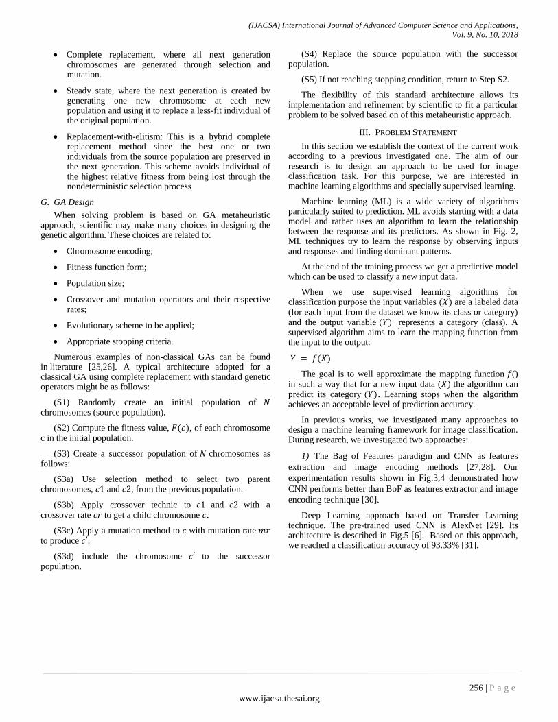
Machine learning (ML) is a wide variety of algorithms particularly suited to prediction. ML avoids starting with a data model and rather uses an algorithm to learn the relationship between the response and its predictors. As shown in Fig. 2, ML techniques try to learn the response by observing inputs and responses and finding dominant patterns.

At the end of the training process we get a predictive model which can be used to classify a new input data.

When we use supervised learning algorithms for classification purpose the input variables are a labeled data (for each input from the dataset we know its class or category) and the output variable represents a category (class). A supervised algorithm aims to learn the mapping function from the input to the output:

The goal is to well approximate the mapping function () in such a way that for a new input data the algorithm can predict its category . Learning stops when the algorithm achieves an acceptable level of prediction accuracy.

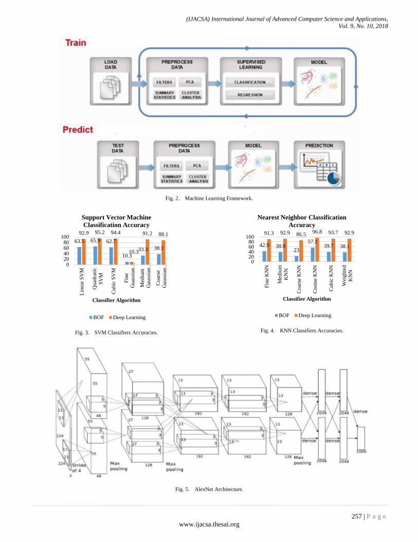
In previous works, we investigated many approaches to design a machine learning framework for image classification. During research, we investigated two approaches:

1) The Bag of Features paradigm and CNN as features

extraction and image encoding methods [27,28]. Our

experimentation results shown in Fig.3,4 demonstrated how

CNN performs better than BoF as features extractor and image

encoding technique [30].

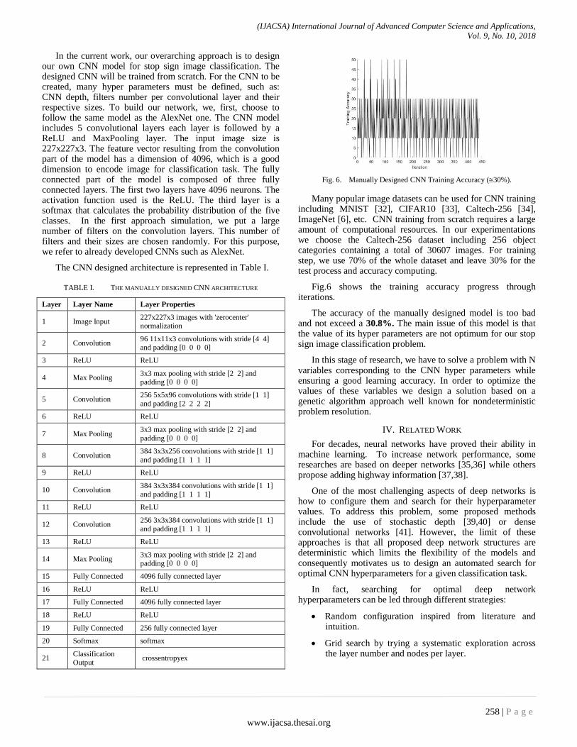
Deep Learning approach based on Transfer Learning technique. The pre-trained used CNN is AlexNet [29]. Its architecture is described in Fig.5 [6]. Based on this approach, we reached a classification accuracy of 93.33% [31].


Vol. 9, No. 10, 2018

257 | P a g e


Fig. 2. Machine Learning Framework.

Fig. 3. SVM Classifiers Accuracies.

Fig. 4. KNN Classifiers Accuracies.

Fig. 5. AlexNet Architecture.

63.5 65.9 62.7

10.3

33.3 38.1

92.9 95.2 94.4

10.3

91.2 88.1

020406080

100

Lin

ear

SV

M

Quad

rati

c

SV

M

Cu

bic

SV

M

Fin

e

Guas

sian

…

Med

ium

Gau

ssia

n…

Co

arse

Gau

ssia

n…

Classifier Algorithm

Support Vector Machine

Classification Accuracy

BOF Deep Learning

42.9 38.9 23

57.1 39.7 38.1

91.3 92.9 86.5 96.8 93.7 92.9

020406080

100

Fin

e K

NN

Med

ium

KN

N

Co

arse

KN

N

Co

sin

e K

NN

Cu

bic

KN

N

Wei

gh

ted

KN

N

Classifier Algorithm

Nearest Neighbor Classification

Accuracy

BOF Deep Learning


Vol. 9, No. 10, 2018

258 | P a g e


In the current work, our overarching approach is to design our own CNN model for stop sign image classification. The designed CNN will be trained from scratch. For the CNN to be created, many hyper parameters must be defined, such as: CNN depth, filters number per convolutional layer and their respective sizes. To build our network, we, first, choose to follow the same model as the AlexNet one. The CNN model includes 5 convolutional layers each layer is followed by a ReLU and MaxPooling layer. The input image size is 227x227x3. The feature vector resulting from the convolution part of the model has a dimension of 4096, which is a good dimension to encode image for classification task. The fully connected part of the model is composed of three fully connected layers. The first two layers have 4096 neurons. The activation function used is the ReLU. The third layer is a softmax that calculates the probability distribution of the five classes. In the first approach simulation, we put a large number of filters on the convolution layers. This number of filters and their sizes are chosen randomly. For this purpose, we refer to already developed CNNs such as AlexNet.

The CNN designed architecture is represented in Table I.

TABLE I. THE MANUALLY DESIGNED CNN ARCHITECTURE

Layer Layer Name Layer Properties

1 Image Input 227x227x3 images with 'zerocenter' normalization

2 Convolution 96 11x11x3 convolutions with stride [4 4] and padding [0 0 0 0]

3 ReLU ReLU

4 Max Pooling 3x3 max pooling with stride [2 2] and padding [0 0 0 0]

5 Convolution 256 5x5x96 convolutions with stride [1 1]

and padding [2 2 2 2]

6 ReLU ReLU

7 Max Pooling 3x3 max pooling with stride [2 2] and

padding [0 0 0 0]



9 ReLU ReLU



11 ReLU ReLU


13 ReLU ReLU


15 Fully Connected 4096 fully connected layer

16 ReLU ReLU


18 ReLU ReLU


20 Softmax softmax

21 Classification Output

crossentropyex

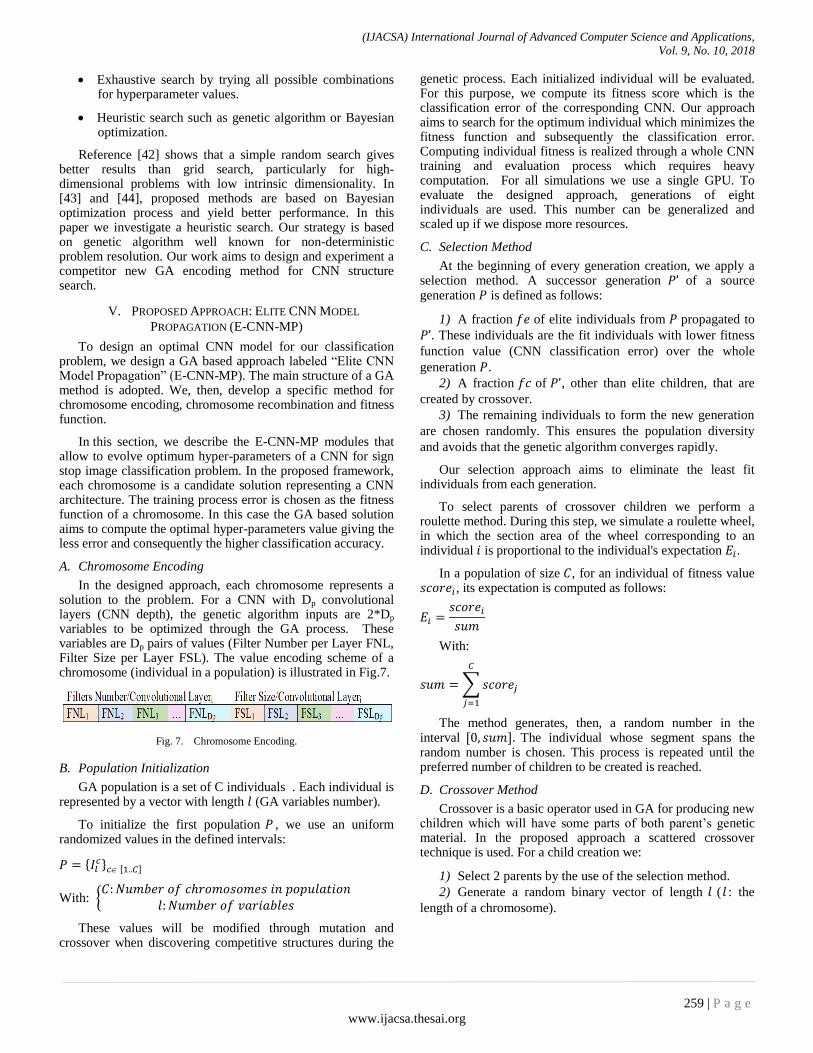
Fig. 6. Manually Designed CNN Training Accuracy (30%).

Many popular image datasets can be used for CNN training including MNIST [32], CIFAR10 [33], Caltech-256 [34], ImageNet [6], etc. CNN training from scratch requires a large amount of computational resources. In our experimentations we choose the Caltech-256 dataset including 256 object categories containing a total of 30607 images. For training step, we use 70% of the whole dataset and leave 30% for the test process and accuracy computing.

Fig.6 shows the training accuracy progress through iterations.

The accuracy of the manually designed model is too bad and not exceed a 30.8%. The main issue of this model is that the value of its hyper parameters are not optimum for our stop sign image classification problem.

In this stage of research, we have to solve a problem with N variables corresponding to the CNN hyper parameters while ensuring a good learning accuracy. In order to optimize the values of these variables we design a solution based on a genetic algorithm approach well known for nondeterministic problem resolution.

IV. RELATED WORK

For decades, neural networks have proved their ability in machine learning. To increase network performance, some researches are based on deeper networks [35,36] while others propose adding highway information [37,38].

One of the most challenging aspects of deep networks is how to configure them and search for their hyperparameter values. To address this problem, some proposed methods include the use of stochastic depth [39,40] or dense convolutional networks [41]. However, the limit of these approaches is that all proposed deep network structures are deterministic which limits the flexibility of the models and consequently motivates us to design an automated search for optimal CNN hyperparameters for a given classification task.

In fact, searching for optimal deep network hyperparameters can be led through different strategies:

Random configuration inspired from literature and intuition.

Grid search by trying a systematic exploration across the layer number and nodes per layer.


Vol. 9, No. 10, 2018

259 | P a g e


Exhaustive search by trying all possible combinations for hyperparameter values.

Heuristic search such as genetic algorithm or Bayesian optimization.

Reference [42] shows that a simple random search gives better results than grid search, particularly for high-dimensional problems with low intrinsic dimensionality. In [43] and [44], proposed methods are based on Bayesian optimization process and yield better performance. In this paper we investigate a heuristic search. Our strategy is based on genetic algorithm well known for non-deterministic problem resolution. Our work aims to design and experiment a competitor new GA encoding method for CNN structure search.

V. PROPOSED APPROACH: ELITE CNN MODEL

PROPAGATION (E-CNN-MP)

To design an optimal CNN model for our classification problem, we design a GA based approach labeled “Elite CNN Model Propagation” (E-CNN-MP). The main structure of a GA method is adopted. We, then, develop a specific method for chromosome encoding, chromosome recombination and fitness function.

In this section, we describe the E-CNN-MP modules that allow to evolve optimum hyper-parameters of a CNN for sign stop image classification problem. In the proposed framework, each chromosome is a candidate solution representing a CNN architecture. The training process error is chosen as the fitness function of a chromosome. In this case the GA based solution aims to compute the optimal hyper-parameters value giving the less error and consequently the higher classification accuracy.

A. Chromosome Encoding

In the designed approach, each chromosome represents a solution to the problem. For a CNN with Dp convolutional layers (CNN depth), the genetic algorithm inputs are 2*Dp variables to be optimized through the GA process. These variables are Dp pairs of values (Filter Number per Layer FNL, Filter Size per Layer FSL). The value encoding scheme of a chromosome (individual in a population) is illustrated in Fig.7.

Fig. 7. Chromosome Encoding.

B. Population Initialization

GA population is a set of C individuals . Each individual is represented by a vector with length (GA variables number).

To initialize the first population , we use an uniform randomized values in the defined intervals:

{ } [ ]

With: {

These values will be modified through mutation and crossover when discovering competitive structures during the

genetic process. Each initialized individual will be evaluated. For this purpose, we compute its fitness score which is the classification error of the corresponding CNN. Our approach aims to search for the optimum individual which minimizes the fitness function and subsequently the classification error. Computing individual fitness is realized through a whole CNN training and evaluation process which requires heavy computation. For all simulations we use a single GPU. To evaluate the designed approach, generations of eight individuals are used. This number can be generalized and scaled up if we dispose more resources.

C. Selection Method

At the beginning of every generation creation, we apply a selection method. A successor generation of a source generation is defined as follows:

1) A fraction of elite individuals from propagated to

. These individuals are the fit individuals with lower fitness

function value (CNN classification error) over the whole

generation .

2) A fraction of , other than elite children, that are

created by crossover.

3) The remaining individuals to form the new generation

are chosen randomly. This ensures the population diversity

and avoids that the genetic algorithm converges rapidly.

Our selection approach aims to eliminate the least fit individuals from each generation.

To select parents of crossover children we perform a roulette method. During this step, we simulate a roulette wheel, in which the section area of the wheel corresponding to an individual is proportional to the individual's expectation .

In a population of size , for an individual of fitness value , its expectation is computed as follows:

𝑠𝑐𝑜𝑟𝑒

With:

∑

The method generates, then, a random number in the interval [ ] The individual whose segment spans the random number is chosen. This process is repeated until the preferred number of children to be created is reached.

D. Crossover Method

Crossover is a basic operator used in GA for producing new children which will have some parts of both parent‟s genetic material. In the proposed approach a scattered crossover technique is used. For a child creation we:

1) Select 2 parents by the use of the selection method.

2) Generate a random binary vector of length ( : the

length of a chromosome).


Vol. 9, No. 10, 2018

260 | P a g e


3) To form the child, we use the gene from the first parent

if the vector value is 1 and the gene from the second parent if

the vector value is 0.

E. Mutation Method

Mutation method is applied on children created by crossover mechanism. The genetic algorithm applies small random changes in each child. Mutation offers population diversity and allows the genetic algorithm to explore a broader space.

Our mutation method is a two-step process:

1) Randomly select the fraction of the child vector to be

mutated according to a probability rate . In practice is

often small. This small value guarantees that the mutation

operator preserves the good properties of a chromosome while

exploring new possibilities. In our experimentation we choose

a equal to .

2) Replace each selected entry (chromosome gene) by a

random number chosen from its corresponding range.

F. Termination of the GA

A GA approach is known to be a stochastic search method. The specification of a convergence criteria is sometimes problematic as the fitness function value may remain unchanged for a number of generations before a superior individual is found. In our approach, we choose to terminate the GA process after an already specified number of generations to avoid materials saturation. Then, we verify the quality of the best individual fitness and if necessary we restart

the GA process with the initialization of a fresh search. The GA Fitness Function.

In this work we are optimizing CNN hyper-parameters for image classification task. Each individual corresponds to a plausible configuration of a CNN. It specifies its number of

filters and their respective sizes. The fitness function or of an individual is computed via the CNN training from scratch

based on an input dataset . In our approach, the classification error is used as individual score.

The input dataset is divided in a and .

The of training is computed as:

The individual

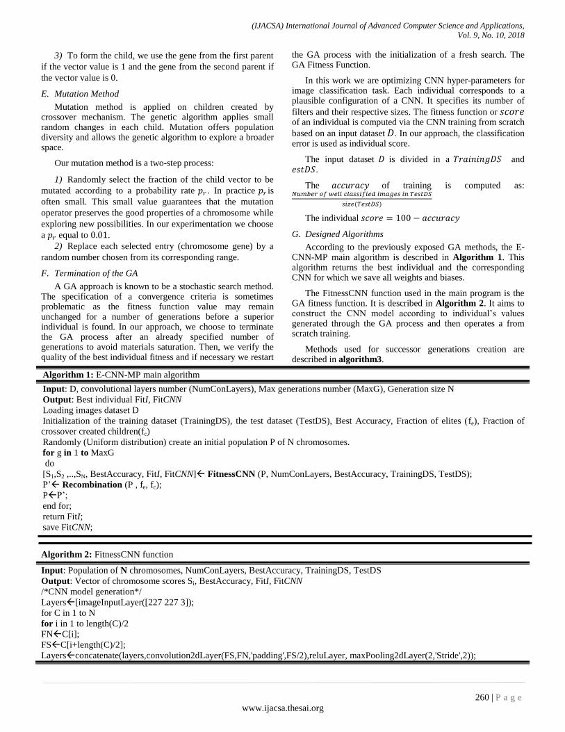
G. Designed Algorithms

According to the previously exposed GA methods, the E-CNN-MP main algorithm is described in Algorithm 1. This algorithm returns the best individual and the corresponding CNN for which we save all weights and biases.

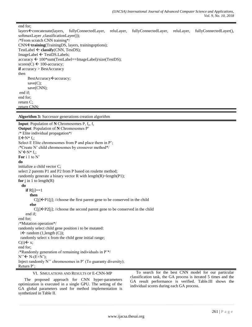
The FitnessCNN function used in the main program is the GA fitness function. It is described in Algorithm 2. It aims to construct the CNN model according to individual‟s values generated through the GA process and then operates a from scratch training.

Methods used for successor generations creation are described in algorithm3.

Algorithm 1: E-CNN-MP main algorithm

Input: D, convolutional layers number (NumConLayers), Max generations number (MaxG), Generation size N

Output: Best individual FitI, FitCNN

Loading images dataset D

Initialization of the training dataset (TrainingDS), the test dataset (TestDS), Best Accuracy, Fraction of elites (fe), Fraction of

crossover created children(fc)

Randomly (Uniform distribution) create an initial population P of N chromosomes.

for g in 1 to MaxG

do

[S1,S2 ,..,SN, BestAccuracy, FitI, FitCNN] FitnessCNN (P, NumConLayers, BestAccuracy, TrainingDS, TestDS);

P‟ Recombination (P , fe, fc);

PP‟;

end for;

return FitI;

save FitCNN;

Algorithm 2: FitnessCNN function

Input: Population of N chromosomes, NumConLayers, BestAccuracy, TrainingDS, TestDS

Output: Vector of chromosome scores Si, BestAccuracy, FitI, FitCNN

/*CNN model generation*/

Layers[imageInputLayer([227 227 3]); for C in 1 to N

for i in 1 to length(C)/2

FNC[i];

FSC[i+length(C)/2];

Layersconcatenate(layers,convolution2dLayer(FS,FN,'padding',FS/2),reluLayer, maxPooling2dLayer(2,'Stride',2));


Vol. 9, No. 10, 2018

261 | P a g e


end for;

layersconcatenate(layers, fullyConnectedLayer, reluLayer, fullyConnectedLayer, reluLayer, fullyConnectedLayer(),

softmaxLayer ,classificationLayer());

/*From scratch CNN training*/

CNNtraining(TrainingDS, layers, trainingoptions);

TestLabel classify(CNN, TestDS);

ImageLabel TestDS.Labels;

accuracy 100*sum(TestLabel==ImageLabel)/size(TestDS);

scores(C) 100-accuracy;

if accuracy > BestAccuracy

then

BestAccuracyaccuracy;

save(C);

save(CNN);

end if;

end for;

return C;

return CNN;

Algorithm 3: Successor generations creation algorithm

Input: Population of N Chromosomes P, fe, fc

Output: Population of N Chromosomes P‟

/* Elite individual propagation*/

EN* fe;

Select E Elite chromosomes from P and place them in P‟;

/*Create N‟ child chromosomes by crossover method*/

N‟N* fc;

For i 1 to N‟

do initialize a child vector C;

select 2 parents P1 and P2 from P based on roulette method;

randomly generate a binary vector R with length(R)=length(P1);

for j in 1 to length(R)

do if R[j]==1

then C[j]P1[j]; //choose the first parent gene to be conserved in the child

else C[j]P2[j]; //choose the second parent gene to be conserved in the child

end if;

end for;

/*Mutation operation*/

randomly select child gene position i to be mutated:

i random (1,length (C));

randomly select x from the child gene initial range;

C(i) x;

end for;

/*Randomly generation of remaining individuals in P‟*/

N‟‟ N-(E+N‟);

Inject randomly N‟‟ chromosomes in P‟ (To guaranty diversity);

Return P‟;

VI. SIMULATIONS AND RESULTS OF E-CNN-MP

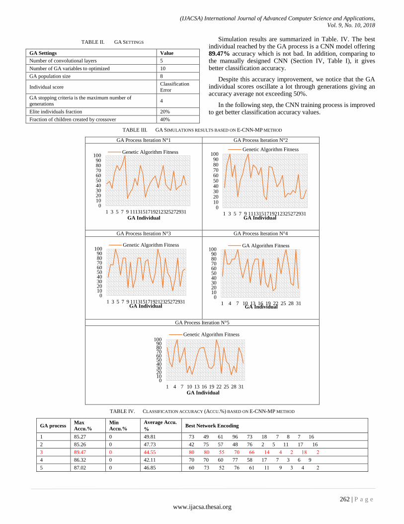
The proposed approach for CNN hyper-parameters optimization is executed in a single GPU. The setting of the GA global parameters used for method implementation is synthetized in Table II.

To search for the best CNN model for our particular classification task, the GA process is iterated 5 times and the GA result performance is verified. Table.III shows the individual scores during each GA process.


Vol. 9, No. 10, 2018

262 | P a g e


TABLE II. GA SETTINGS

GA Settings Value

Number of convolutional layers 5

Number of GA variables to optimized 10

GA population size 8

Individual score Classification

Error

GA stopping criteria is the maximum number of

generations 4

Elite individuals fraction 20%

Fraction of children created by crossover 40%

Simulation results are summarized in Table. IV. The best individual reached by the GA process is a CNN model offering 89.47% accuracy which is not bad. In addition, comparing to the manually designed CNN (Section IV, Table I), it gives better classification accuracy.

Despite this accuracy improvement, we notice that the GA individual scores oscillate a lot through generations giving an accuracy average not exceeding 50%.

In the following step, the CNN training process is improved to get better classification accuracy values.

TABLE III. GA SIMULATIONS RESULTS BASED ON E-CNN-MP METHOD

GA Process Iteration N°1 GA Process Iteration N°2


GA Process Iteration N°5

TABLE IV. CLASSIFICATION ACCURACY (ACCU.%) BASED ON E-CNN-MP METHOD

GA process Max

Accu.%

Min

Accu.%

Average Accu.

% Best Network Encoding

1 85.27 0 49.81 73 49 61 96 73 18 7 8 7 16

2 85.26 0 47.73 42 75 57 48 76 2 5 11 17 16

3 89.47 0 44.55 80 80 55 70 66 14 4 2 18 2

4 86.32 0 42.11 70 70 60 77 58 17 7 3 6 9

5 87.02 0 46.85 60 73 52 76 61 11 9 3 4 2

0102030405060708090

100

1 4 7 10 13 16 19 22 25 28 31GA Individual

GA Algorithm Fitness

0102030405060708090

100

1 3 5 7 9 1113151719212325272931GA Individual

Genetic Algorithm Fitness

0102030405060708090

100

1 3 5 7 9 1113151719212325272931

GA Individual


0102030405060708090

100

1 3 5 7 9 1113151719212325272931GA Individual


0102030405060708090

100

1 4 7 10 13 16 19 22 25 28 31GA Individual



Vol. 9, No. 10, 2018

263 | P a g e


VII. ENHANCED E-CNN-MP

Many methods are proposed to optimize a deep neural network training. Some of them try to reduce the sensitivity to network initialization. Among these enhanced initialization schemes, we quote: Xavier Initialization [45], Theoretically Derived Adaptable Initialization [46], Standard Fixed Initialization [6], etc. However, researches demonstrate that these methods have some limits. In fact, Xavier Initialization is not suited for rectification-based nonlinear activations CNN. Although, Theoretically Derived Adaptable Initialization method improves convergence characteristics, it is not confirmed that it led to better accuracy. It is also proven that Standard Fixed Initialization delays convergence because of the gradients magnitude or activations in a deep network final layers [7,47].

Other methods are interested to reduce the internal covariate shift phenomenon produced by variations in the distribution of each layer‟s inputs due to parameters changes in the previous layer. An “internal covariate shift” problem can dramatically affect CNN training [48]. In fact, during training process when the data is flowing through the CNN, their values are adjusted by the weights and parameters. This procedure makes sometimes the data too big or too small. To largely avoid this problem, the idea is to normalize the data in each mini-batch and not only for input data during the preprocessing

step [48]. For each input channel across a mini-batch, activation normalization is, first, performed by subtracting the mini-batch mean and dividing by the mini-batch standard deviation. Input is, then, shifted by a learnable offset β and scaled by a learnable scale factor γ.

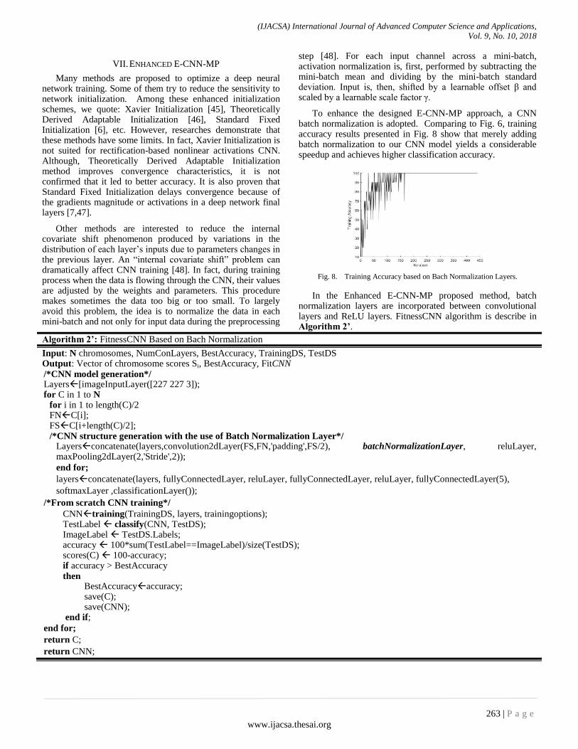
To enhance the designed E-CNN-MP approach, a CNN batch normalization is adopted. Comparing to Fig. 6, training accuracy results presented in Fig. 8 show that merely adding batch normalization to our CNN model yields a considerable speedup and achieves higher classification accuracy.

Fig. 8. Training Accuracy based on Bach Normalization Layers.

In the Enhanced E-CNN-MP proposed method, batch normalization layers are incorporated between convolutional layers and ReLU layers. FitnessCNN algorithm is describe in Algorithm 2’.

Algorithm 2’: FitnessCNN Based on Bach Normalization

Input: N chromosomes, NumConLayers, BestAccuracy, TrainingDS, TestDS Output: Vector of chromosome scores Si, BestAccuracy, FitCNN /*CNN model generation*/ Layers[imageInputLayer([227 227 3]); for C in 1 to N

for i in 1 to length(C)/2 FNC[i]; FSC[i+length(C)/2]; /*CNN structure generation with the use of Batch Normalization Layer*/

Layersconcatenate(layers,convolution2dLayer(FS,FN,'padding',FS/2), batchNormalizationLayer, reluLayer, maxPooling2dLayer(2,'Stride',2));

end for;

layersconcatenate(layers, fullyConnectedLayer, reluLayer, fullyConnectedLayer, reluLayer, fullyConnectedLayer(5),

softmaxLayer ,classificationLayer());

/*From scratch CNN training*/

CNNtraining(TrainingDS, layers, trainingoptions); TestLabel classify(CNN, TestDS); ImageLabel TestDS.Labels; accuracy 100*sum(TestLabel==ImageLabel)/size(TestDS); scores(C) 100-accuracy; if accuracy > BestAccuracy then BestAccuracyaccuracy; save(C); save(CNN); end if;

end for;

return C;

return CNN;


Vol. 9, No. 10, 2018

264 | P a g e


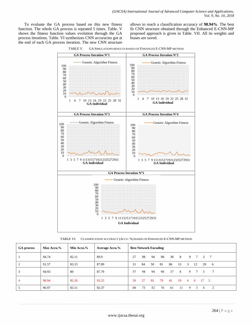
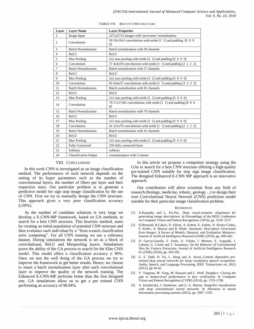
To evaluate the GA process based on this new fitness function. The whole GA process is repeated 5 times. Table. V shows the fitness function values evolution through the GA process iterations. Table. VI synthesizes CNN accuracies got at the end of each GA process iteration. The new CNN structure

allows to reach a classification accuracy of 98.94%. The best fit CNN structure obtained through the Enhanced E-CNN-MP proposed approach is given in Table. VII. All its weights and biases are saved.

TABLE V. GA SIMULATIONS RESULTS BASED ON ENHANCED E-CNN-MP METHOD



GA Process Iteration N°5

TABLE VI. CLASSIFICATION ACCURACY (ACCU. %) BASED ON ENHANCED E-CNN-MP METHOD

GA process Max Accu.% Min Accu.% Average Accu.% Best Network Encoding

1 94.74 82.11 89.9 57 98 94 98 38 8 9 7 3 7

2 91.57 83.15 87.89 31 84 50 81 86 13 3 12 20 6

3 94.93 80 87.79 57 98 94 98 37 8 9 7 3 7

4 98.94 85.26 93.25 59 37 81 79 41 19 4 6 17 5

5 96.97 83.11 92.37 60 73 52 76 61 11 9 3 4 2

0102030405060708090

100

1 3 5 7 9 1113151719212325272931

GA Individual


0102030405060708090

100

1 3 5 7 9 1113151719212325272931GA Individual


0102030405060708090

100

1 3 5 7 9 1113151719212325272931GA Individual


0102030405060708090

100

1 4 7 10 13 16 19 22 25 28 31

GA Individual


0102030405060708090

100

1 4 7 10 13 16 19 22 25 28 31GA Individual



Vol. 9, No. 10, 2018

265 | P a g e


TABLE VII. BEST FIT CNN STRUCTURE

Layer Layer Name Layer Properties

1 Image Input 227x227x3 images with 'zerocenter' normalization

2 Convolution 59 19x19x3 convolutions with stride [1 1] and padding [9 9 9

9]

3 Batch Normalization Batch normalization with 59 channels

4 ReLU ReLU




8 ReLU ReLU




12 ReLU ReLU


14 Convolution 79 17x17x81 convolutions with stride [1 1] and padding [8 8 8

8]


16 ReLU ReLU




20 ReLU ReLU



23 Softmax softmax

24 Classification Output crossentropyex with 5 classes

VIII. CONCLUSIONS

In this work CNN is investigated as an image classification method. The performance of such network depends on the setting of its hyper parameters such as the number of convolutional layers, the number of filters per layer and their respective sizes. Our particular problem is to generate a predictive model for sign stop image classification by the use of CNN. First we try to manually design the CNN structure. This approach gives a very poor classification accuracy

(30%).

As the number of candidate solutions is very large we develop a E-CNN-MP framework, based on GA methods, to search for a best CNN structure. This heuristic method, starts by creating an initial population of potential CNN structure and then evaluates each individual by a “from scratch classification error computing”. For all CNN training we use a reference dataset. During simulations the network is set as a block of convolutional, ReLU and Maxpooling layers. Simulations prove the ability of the GA process to search for the Elite CNN

model. This model offers a classification accuracy 90%. Once we test the well doing of the GA process we try to improve the framework to get better results. Hence, we choose to insert a batch normalization layer after each convolutional layer to improve the quality of the network training. The Enhanced E-CNN-MP performs better than the first designed one. GA simulations allow us to get a pre trained CNN performing an accuracy of 98.94%.

In this article we propose a competitor strategy using the GAs to search for a best CNN structure offering a high-quality pre-trained CNN suitable for stop sign image classification. The designed Enhanced E-CNN MP approach is an innovative approach.

Our contribution will allow scientists from any field of research (biology, medicine, robotic, geology ...) to design their own Convolutional Neural Network (CNN) prediction model suitable for their particular image classification problem.

REFERENCES

[1] A.Karpathy and L. Fei-Fei,. Deep visual-semantic alignments for generating image descriptions. In Proceedings of the IEEE Conference on Computer Vision and Pattern Recognition. (2016), pp. 3128–3137.

[2] R.Bernardi, R.Cakici, D. Elliott, A. Erdem, E. Erdem, N. Ikizler-Cinbis, F. Keller, A. Muscat and B. Plank. Automatic Description Generation from Images: A Survey of Models, Datasets, and Evaluation Measures. Journal of Artificial Intelligence Research (JAIR) (2016), pp. 409-442.

[3] D. Garcia-Gasulla, F. Parès, A. Vilalta, J. Moreno, E. Ayguadé, J. Labarta, U. Cortés and T. Suzumura. On the Behavior of Convolutional Nets for Feature Extraction. Journal of Artificial Intelligence Research 61 (JAIR) (2018), pp. 563-592.

[4] G. E. Dahl, D. Yu, L. Deng and A. Acero,.Context dependent pre-trained deep neural networks for large vocabulary speech recognition. Audio, Speech, and Language Processing, IEEE Transactions on, 20(1) (2012), pp.30-42.

[5] Y. Taigman, M. Yang, M. Ranzato and L. Wolf. Deepface: Closing the gap to human-level performance in face verification. In Computer Vision and Pattern Recognition (CVPR) (2014), pp. 1701-1708.

[6] A. Krizhevsky, I. Sutskever, and G. E. Hinton. ImageNet classification with deep convolutional neural networks. In Advances in neural information processing systems (2012), pp. 1097–1105.


Vol. 9, No. 10, 2018

266 | P a g e


[7] K. Simonyan and A. Zisserman. Very Deep Convolutional Networks for Large-Scale Image Recognition. International Conference on Learning Representations. (2014).

[8] K. He, X. Zhang, S.Ren and J.Sun Deep Residual Learning for Image Recognition. Computer Vision and Pattern Recognition. (2016).

[9] F. M. Ham and I. Kostanic. Principles of Neurocomputing for Science and Engineering. McGraw-Hill Higher Education. (2000).

[10] Y. LeCun, Y. Bengio and G. Hinton. Deep Learning. Nature521(7553) (2015), pp. 436–444. doi:10.1038/nature14539.

[11] S. Srinivas, R. K. Sarvadevabhatla, K. R. Mopuri, N. Prabhu, S. S.Kruthiventi and R. V. Babu, A taxonomy of deep convolutional neural nets for computer vision. (2016). arXiv 1601.06615.

[12] C. Szegedy, W. Liu, Y. Jia, P. S. Sermanet, D. Anguelov, D. Erhan, V. Vanhoucke and A. Rabinovich. Going Deeper with Convolutions (2014). arXiv:1409.4842.

[13] M. D. Zeiler, and R. Fergus. Visualizing and Understanding Convolutional Networks (2013). arXiv:1311.2901v3.

[14] A. W. Harley. An Interactive Node-Link Visualization of Convolutional Neural Networks. In ISVC (2015), pp. 867-877.

[15] A. W. Dumoulin, and F. Visin, A guide to convolution arithmetic for deep learning (2016). arXiv:1603.07285v1.

[16] K. Jarrett, K. Kavukcuoglu, M. Ranzato and Y. LeCun, What is the best multi-stage architecture for object recognition?. In Proceedings of the IEEE International Conference on Computer Vision (2009), pp. 2146–2153.

[17] V. Nair and G. Hinton. Rectified linear units improve restricted boltzmann machines. In Proceedings of International Conference on Machine Learning (2010), pp. 807–814.

[18] D. Nguyen and B. Widrow. Improving the learning speed of 2-layer neural networks by choosing initial values of the adaptive weights. In International Joint Conference on Neural Networks (1990), pp. 21–26 vol.3.

[19] M. Norouzi, M. Ranjbar and G.Mori. Stacks of convolutional restricted boltzmann machines for shift-invariant feature learning. In IEEE Transactions on Conference on Computer Vision and Pattern Recognition (2009), pp. 2735–2742.

[20] B. Xu, N. Wang, T. Chen and M. Li. Empirical evaluation of rectified activations in convolutional network (2015). arXiv 1505.00853v2.

[21] W. Liu, Y. Wen, M. Scut, Z. Yu and M. Yang. Large-margin softmax loss for convolutional neural networks. In Proceedings of the 33rd International Conference Machine Learning (2016), pp. 507–516.

[22] G. Brandon and A. Sigberto. Real-time American Sign Language Recognition with Convolutional Neural Networks. Stanford Vision Lab, (2016).

[23] J. McCall. Genetic algorithms for modelling and optimization. Journal of Computational and Applied Mathematics (2005), Volume 184, pp. 205-222.

[24] T. Bäck, D. B. Fogel, and Z. Michalewicz. Handbook of Evolutionary Computation. IOP Publishing. (1997).

[25] L. Davis. Handbook of Genetic Algorithms. Van Nostrand Reinhold, New York (1991).

[26] Z. Michaelewicz. Genetic Algorithms + Data structures = Evolution Programs (third ed.), (Springer, Berlin ,1999).

[27] S. Loussaief and A. Abdelkrim. Machine Learning Framework for Image Classification. In Sciences of Electronics, Technologies of Information and Telecommunications, SETIT 2016.

[28] S. Loussaief and A. Abdelkrim. Machine Learning Framework for Image Classification. In, Advances in Sciences, Technology and Engineering Systems Journal (2018), Vol.3 No. 1, 01-10, ISSN: 2415-6698.

[29] J. Donahue, Y. Jia, O. Vinyals, J. Hoffman, N. Zhang, E. Tzeng and T. Darrell. A deep convolutional activation feature for generic visual recognition (2013), CoRR, abs/1310.1531.

[30] S. Loussaief and A. Abdelkrim. Deep Learning vs. Bag of Features in Machine Learning for Image Classification. In International Conference on Advanced Systems and Electrical Technologies, IC‟ASET 2018.

[31] N. Jmour, S. Loussaief and A. Abdelkrim. Convolutional Neural Networks for image classification. In International Conference on Advanced Systems and Electrical Technologies, IC‟ASET 2018.

[32] Y. LeCun, L. Bottou, Y. Bengio, and P. Haffner. Gradientbased Learning Applied to Document Recognition. Proceedings of the IEEE, 86(11):2278–2324, 1998.

[33] A. Krizhevsky and G. Hinton. Learning Multiple Layers of Features from Tiny Images. Technical Report, University of Toronto, 1(4):7, 2009.

[34] G. Griffin, A. Holub and P. Perona. Caltech-256 Object Category Dataset. Mars 2007.

[35] K. Simonyan and A. Zisserman. Very Deep Convolutional Networks for Large-Scale Image Recognition. International Conference on Learning Representations, 2014.

[36] C. Szegedy, W. Liu, Y. Jia, P. Sermanet, S. Reed, D. Anguelov, D. Erhan, V. Vanhoucke, and A. Rabinovich. Going Deeper with Convolutions. Computer Vision and Pattern Recognition, 2015.

[37] K. He, X. Zhang, S. Ren, and J. Sun. Deep Residual Learning for Image Recognition. Computer Vision and Pattern Recognition, 2016.

[38] S. Zagoruyko and N. Komodakis. Wide Residual Networks. arXiv preprint, arXiv: 1605.07146, 2016.

[39] L. Xie, J. Wang, W. Lin, B. Zhang, and Q. Tian. Towards Reversal-Invariant Image Representation. International Journal on Computer Vision, 2016.

[40] G. Huang, Y. Sun, Z. Liu, D. Sedra, and K.Weinberger. Deep Networks with Stochastic Depth. European Conference on Computer Vision, 2016.

[41] G. Huang, Z. Liu, and K. Weinberger. Densely Connected Convolutional Networks. arXiv preprint, arXiv:1608.06993, 2016.

[42] J. Bergstra and Y. Bengio. Random search for hyper-parameter optimization. JMLR, 13(1):281–305, 2012.

[43] J. Bergstra, D. Yamins, and D.D. Cox. Making a science of model search: Hyperparameter optimization in hundreds of dimensions for vision architectures. In Proc. Of ICML, pages 115–123, 2013.

[44] F. Hutter, H. Hoos, and K. Leyton-Brown. Sequential model-based optimization for general algorithm configuration. In Proc. of LION, pages 507–523. Springer, 2011.

[45] X. Glorot and Y. Bengio. Understanding the difficulty of training deep feedforward neural networks. In Proceedings of the 13th International Conference on Artificial Intelligence and Statistics (2010), pp. 249–256.

[46] K. He, X. Zhang, S. Ren and J. Sun. Deep residual learning for image recognition (2015). arXiv 1512.03385.

[47] D. Mishkin and J. Matas. All you need is a good init. In Proceedings of the 4th International Conference on Learning Representations (2016), pp. 1–13.

[48] S. Ioffe and C. Szegedy. Batch Normalization: Accelerating Deep Network Training by Reducing Internal Covariate(2015). arXiv:1502.03167

Convolutional Neural Network Hyper-Parameters Optimization ...€¦ · applications, Convolutional...

Documents

Transcript of Convolutional Neural Network Hyper-Parameters Optimization ...€¦ · applications, Convolutional...