Convex optimization for finite horizon robust covariance control of

linear stochastic systems

Georgios Kotsalis, Guanghui Lan, Arkadi Nemirovski ∗

July 2, 2020

Abstract

This work addresses the finite-horizon robust covariance control problem for discrete-time,partially observable, linear system affected by random zero mean noise and deterministic butunknown disturbances restricted to lie in what is called ellitopic uncertainty set (e.g., finite in-tersection of centered at the origin ellipsoids/elliptic cylinders). Performance specifications areimposed on the random state-control trajectory via averaged convex quadratic inequalities, linearinequalities on the mean, as well as pre-specified upper bounds on the covariance matrix. For thisproblem we develop a computationally tractable procedure for designing affine control policies,in the sense that the parameters of the policy that guarantees the aforementioned performancespecifications are obtained as solutions to an explicit convex program. Our theoretical findingsare illustrated by a numerical example.

Keywords: robust optimization, convex programming, multistage minimax

AMS 2000 subject classification: 90C47,90C22, 49K30, 49M29

1 Introduction

The standard finite-horizon covariance control problem pertains to designing a feedback control policyfor a linear dynamical system affected by zero mean Gaussian disturbances that will steer an initialGaussian random vector (close to) to a prescribed terminal one. Such stochastic constraints aim toreduce conservativeness by requiring from the feedback law the imposition of a desired probabilitydistribution profile on the state-control trajectory. The problem has been studied for linear dynamicalsystems under full-state feedback in continuous [1], [2], [3], as well as discrete-time settings [4], [5].

In this work we consider a robust version of the finite horizon discrete-time covariance controlproblem under partial observation. We are given a discrete-time, linear system, referred to as (S),with state space description

x0 = z + s0

xt+1 = At xt + Bt ut + B(d)t dt + B

(s)t et,

yt = Ct xt + D(d)t dt + D

(s)t et, t = 0, 1, 2, . . . , N,

∗H. Milton Stewart School of Industrial & Systems Engineering, Georgia Institute of Technology, Atlanta, GA 30332.(email: gkotsalis3@gatech.edu, george.lan@isye.gatech.edu, arkadi.nemirovski@isye.gatech.edu).

1

arX

iv:2

007.

0013

2v1

[m

ath.

OC

] 3

0 Ju

n 20

20

where at time t, xt ∈ Rnx is the state, ut ∈ Rnu the control input, yt ∈ Rny the observableoutput, dt ∈ Rnd the bounded but unknown exogenous disturbance, while et ∈ Rne is the stochasticexogenous disturbance. The matrices appearing in the state space description of (S) are known andhave compatible dimensions. In the sequel we treat the initial state x0 as an exogenous factor withdeterministic component z and a stochastic one s0. The stochastic exogenous factors form a randomdisturbance vector

ε = [s0; e0; ...; eN−1] 1

and is assumed to have zero mean and known covariance matrix Π. The deterministic exogenousfactors form the deterministic disturbance vector

ζ = [z; d0; ...; dN−1]

which is “unknown but bounded” – known to run through a given uncertainty set Z .Our goal is to achieve a desired system behavior on the finite horizon t = 0, 1, . . . , N , by designing

an appropriate non-anticipative affine control law of the form

ut = gt +t∑i=0

Gti yi, t = 0, 1, . . . , N − 1.

where gt and Gti are vectors and matrices of appropriate sizes parameterizing the control policy. Per-formance requirements on (S) are expressed in terms of the resulting random state-control trajectory

w = [x1; ...; xN ; u0; ...; uN−1].

Specifically the desired behavior is modeled by a system of convex constraints on the covariancematrix Σw of the trajectory of the form

∀ζ ∈ Z , Qi Σw QTi � Λi, i = 1, . . . , Ic,

where the parameters {Λi,Qi}i∈{1,...,Ic} of compatible dimensions are given. We will also consideraveraged convex quadratic inequality constraints on the state-control trajectory

∀ζ ∈ Z , E[〈Ai (w − βi), (w − βi)〉 ≤ γi, i = 1, . . . , Iq,

where again the parameters {Ai, βi, γi}i∈{1,...,Iq} defining the inequalities are assumed to be part ofthe problem specification.

These two systems of inequalities allow the designer to express among other requirements also thatthe mean µw of the state-control trajectory is confined in a pre-specified set, while the covariance Σw

does not to exceed a given upper bound, for all realization of the deterministic disturbances ζ ∈ Z .In this paper we develop under some assumptions on Z , that are for instance satisfied when Z is

the intersection of K concentric ellipsoids/elliptic cylinders, a computationally tractable procedurefor designing affine control policies, in the sense that the parameters of the policy that guarantees theaforementioned performance specifications at a certain level of uncertainty are obtained as solutionsto an explicit convex program.

1Here and in what follows we use “MATLAB notation:” expressions like z = [u1;u2; ...;uk] (z = [u1, u2, ..., uk])mean that vector/matrix z is obtained from blocks ui by writing u2 beneath u1, u3 beneath u2, etc. (resp. writing u2

to the right of u1, u3 to the right of u2, etc.)

2

Our work expands on the previous investigations on finite horizon covariance control [1]-[5] byaddressing the robustness issue and the possibility that the full state may not be available, thereforeenabling the steering of the state-control trajectory density in the presence of disturbances underpartial observation.

Our contribution to the robust control literature lies in the fact that we provide a tractablecomputational framework to address the control design problem for a wide class of uncertainty setsZ called ellitopes, a concept that was introduced in [6]. Many interesting uncertainty models fallin the class of ellitopes, including intersection of ellipsoids and elliptic cylinders, box constraints,as well as the case when the origin of the exogenous disturbances are discretized continuous-timesignals that satisfy Sobolev-type smoothness constraints. In terms of a tractable formulation weexpand considerably on the the standard finite-horizon robust control problem utilizing the inducedl2 gain as a sensitivity measure, where the uncertainty set consists of a single ellipsoid (see, e.g., [7],[8], [9] and references therein).

From a historical perspective the covariance control problem in the infinite-horizon case goesback to the original papers on the steady state assignment problem [11], [12], see also [13] and thereferences therein. The investigation of the finite horizon case was initiated in [1], where the optimalcovariance steering problem was considered under the assumption that both input and noise channelsare identical; this requirement was relaxed in [2]. The work in [4] addressed the optimal covariancecontrol problem with constraints on input, while [5] included chance constraints in the formulationas well.

This paper considers the finite horizon covariance control problem under partial observationwhile focusing on the issue of robustness. Essential to our developments is a key result derived in[6], specifically, the quantification of the approximation ratio of the semidefinite relaxation bound onthe maximum of a quadratic form over an ellitope.

Another key ingredient to our work is the consideration of affine policies that are functions ofthe so-called “purified outputs”. This re-parametrization of the set of policies induces a bi-affinestructure in the state and control variables that can further be exploited via robust optimizationtechniques. While the specifics are different, in terms of its effect, this step of passing to purifiedoutputs is akin to the Q-parametrization [14],[15] in infinite horizon control problems.

Control design in terms of purified outputs was introduced in [16], where the authors investigatedthe finite-horizon robust control problem for deterministic linear systems affected by set boundeddisturbances and linear constraints imposed on the state-control trajectory. In this work we replacelinear constraints with convex quadratic ones, while still allowing for a rich class of uncertainty sets,namely ellitopes. The price one pays for this generalization is that the resulting convex formulationfor the affine policy design amounts to a semidefinite program rather than linear programminglinear/convex quadratic programming programs yielded by [16].

The appealing feature of tractability when restricting ourselves to affine policies comes at thecost of potential conservatism. In the scalar case, under the assumption of deterministic dynamics,the optimality of affine policies for a class of robust multistage optimization problems subject toconstraints on the control variables was proven in [17]. The degree of suboptimality of affine policieswas investigated computationally in [18] and [19]. The former reference employs the sum of squaresrelaxation, while the latter efficiently computes the suboptimality gap by invoking linear decisionrules in the dual formulation as well. Further applications of affine policies can be found in stochasticprogramming settings [20], [21] and in the area of robust model predictive and receding horizoncontrol [22], [23], [24], [25].

3

The paper is organized as follows. In Section 2 we introduce the formal problem statement in-cluding the notion of ellitopic uncertainty sets, which is new to the control literature. The theoreticaldevelopments that lead to a computationally tractable formulation are described in Section 3, whileSection 4 contains an extension to the even wider family of uncertainty sets namely spectratopes.The paper concludes with a numerical example in Section 5. Some technical proofs are relegated tothe Appendix.

1.1 Notation

The set of real numbers is denoted by R. All vectors are column vectors. The transpose of thecolumn vector x ∈ Rn is written as xT and [x]i refers to the i-th entry of x, while [A]i,j refers to the(i, j)-th entry of the matrix A ∈ Rn×m.

The space of symmetric n× n matrices is denoted Sn, the cone of positive semidefinite matricesfrom Sn is denoted Sn+, its interior Sn++, and the relations A � B, A � B stand for A−B ∈ Sn+, resp.,A− B ∈ Sn++. For x, y ∈ Rn, 〈x, y〉 denotes the inner product of the two vectors. A sum (product)of n× n matrices over an empty set of indices is the n× n zero (identity) matrix.

2 Problem Statement

In this section we elaborate on the problem statement described in the introduction, by expandingon the concept of affine policies in purified outputs, the ellitopic uncertainty sets, as well as give somefurther justification on the use of averaged quadratic inequalities on random state-control trajectoryas part of the performance specifications.

2.1 System dynamics and affine control laws

We consider a discrete-time, linear system, referred to as (S), with state space description

x0 = z + s0,

xt+1 = At xt + Bt ut + B(d)t dt + B

(s)t et (1)

yt = Ct xt + D(d)t dt + D

(s)t et, 0 ≤ t ≤ N − 1.

where xt ∈ Rnx are states, ut ∈ Rnu are controls, yt ∈ Rny are observable outputs. The system isaffected by two kinds of exogenous factors:– “uncertain but bounded” deterministic factors z ∈ Rnx , dt ∈ Rnd , 0 ≤ t ≤ N−1 which we assembleinto a single deterministic disturbance vector

ζ = [z; d0; ...; dN−1] ∈ Rnζ , nζ = nx + ndN ;

– stochastic factors s0 ∈ Rnx , et ∈ Rne , 0 ≤ t ≤ N − 1, which we assemble into a single stochasticdisturbance vector

ε = [s0; e0; ...; eN−1] ∈ Rnε , nε = nx + neN.

We assume that

• the matrices At, Bt, ..., D(s)t are known for all t, 0 ≤ t ≤ N − 1,

4

• deterministic disturbance ζ takes its values in a given uncertainty set Z ⊂ Rnx+ndN (of struc-ture to be specified later),

• the stochastic disturbance ε is random vector with zero mean and known in advance covariancematrix Π.

Performance specifications will be expressed via constraints on the random state-control trajec-tory w and its first two moments. The trajectory is obtained by stacking the state and the controlvectors of various time instances:

x = [x1; ...; xN ] ∈ RnxN , u = [u0; ...; uN−1] ∈ RnuN , w = [x; u] ∈ Rnw , nw = (nx + nu)N (2)

We will restrict ourselves to casual (non-anticipative) affine control laws. The classical output-based (OB) affine policy is

ut = gt +t∑i=0

Gti yi, 0 ≤ t ≤ N − 1; (3)

such a policy is specified by the collection of parameters

θ = {gt, Gtj}j≤t,t≤N−1, gt ∈ Rnu , Gtj ∈ Rnu×nx . (4)

When employing an (OB) affine policy with parameters θ the state-control trajectory is affine inthe initial state and disturbances while highly nonlinear in the parameters θ of the policy [16]. Anessential step towards developing a computationally tractable control design formulation is passingto deterministic control policies that are affine in the purified outputs of the system, i.e. purified-output-based (POB) control laws. To introduce this concept suppose first that the system (S) iscontrolled by some causal policy

ut = φt(y0, . . . ,yt), 0 ≤ t ≤ N − 1.

We consider now the evolution of a disturbance free system starting from rest, with state spacedescription

x0 = 0,

xt+1 = At xt + Bt ut,

yt = Ct xt, 0 ≤ t ≤ N − 1. (5)

The dynamics in (5) can be run in “on-line” fashion given that the decision maker knows the alreadycomputed control values. The purified outputs vt are the differences of the outputs of the actualsystem (1) and the outputs of the auxiliary system (5):

vt = yt − yt, 0 ≤ t ≤ N − 1. (6)

The term “purified” stems from the fact that the outputs (6) do not depend on the particular choiceof control policy. This circumstance is verified by introducing the signal

δt = xt − xt, 0 ≤ t ≤ N − 1,

5

and observing that the purified outputs can also be obtained by combining (1), (5), (6) and thedefinition of δt as the outputs of the system with state space description

δ0 = z + s0,

δt+1 = At δt + B(d)t dt + B

(s)t et,

vt = Ct δt + D(d)t dt + D

(s)t et, 0 ≤ t ≤ N − 1. (7)

Thus, purified outputs are known in advance affine functions of disturbances ζ, ε. Furthermore attime instant t, when the decision on the control value ut is to be made, we already know the purifiedoutputs v0, v1, . . . , vt. An affine POB policy is, by definition, of the form

ut = ht +t∑i=0

Hti vi, 0 ≤ t ≤ N − 1; (8)

such a policy is specified by collection of control parameters

χ = {ht, Htj}0≤j≤t≤N−1, ht ∈ Rnu , Ht

j ∈ Rnu×nx . (9)

It is proved in [16] that as far as the “behaviour” of the controlled system is concerned, the OB andPOB control laws are equivalent. Specifically, equipping the open loop system (S) with an affineoutput-based control policy specified by the parameters θ, the state-control trajectory becomes anaffine function of the disturbances [ζ; ε]:

w = Xθ (ζ, ε)

for some vector-valued affine in its argument [ζ; ε] function Xθ(·). Equipping (S) with an affine POBcontrol policy specified by the parameters χ, the state-control trajectory becomes an affine functionof the disturbances:

w = Wχ (ζ, ε)

for some vector-valued affine in its argument [ζ; ε] function Wχ(·). It is shown in [16] that forevery θ there exists χ such that Xθ(·) ≡ Wχ(·), and vice versa. It follows that as far as generaltype affine output based/purified output based control policies are concerned, and whenever thedesign specifications are expressed in terms of the state-control trajectory (e.g., by imposing on theexpectation of the trajectory w.r.t. ε inequalities which should be satisfied for all realizations ζ ∈ Z ),we lose nothing by restricting ourselves to affine POB controls policies. This is what we intend to do,the reason being that, as is easily seen (and is shown in [16]), the mapping (χ, [ζ; ε])→Wχ ([ζ; ε]) isbi-affine: affine in χ when [ζ; ε] is fixed, and affine in [ζ; ε] when χ is fixed. In other words,

w = Wχ(ζ, ε) ≡ Z[χ][ζ; 1] + E[χ]ε

[Z[χ] and E[χ]: affine in χ](10)

As we shall see, this bi-affinity is crucial in the process of reducing the control design to a computa-tionally tractable problem. Note that the affine matrix-valued functions Z[χ], E[χ] are readily given

by the matrices At, ..., D(s)t , 0 ≤ t ≤ N − 1, participating in (1).

6

2.2 Ellitopic uncertainty sets

The issue of computational tractability in the ensuing formulation hinges upon the postulated struc-ture of the uncertainty set. Specifically, we will consider a family of uncertainty sets D [ρ], a single-parameter family of similar to each other ellitopes2 parameterized by the uncertainty level ρ ≥ 0:

D [ρ] = {x ∈ Rnζ | ∃(z ∈ Rn, t ∈ T ) : x = Pz, 〈Skz, z〉 ≤ [t]kρ, k = 1, . . . ,K}, (11)

where

• ρ > 0, P is an nζ × n matrix, and Sk, 1 ≤ k ≤ K, are n× n matrices with Sk � 0,∑

k Sk � 0,

• T is a nonempty computationally tractable convex compact subset of RK+ intersecting theinterior of RK+ and such that T is monotone, meaning that if 0 ≤ t ≤ t′ and t′ ∈ T then t ∈ T .

Note that D [ρ] =√ρD [1].

The particular choice of uncertainty description encompasses many interesting cases even from apurely robust control perspective in the absence of stochastic noises in a unifying framework.

• When K = 1, T = [0, 1] and Q1 � 0, D [ρ] reduces to a family of proportional to each otherellipsoids. This class of uncertainty sets is employed in the standard finite-horizon robustcontrol problem utilizing the induced l2 gain as a sensitivity measure.

• When K ≥ 1, T = [0, 1]K , D [ρ] is the linear image, under linear mapping z → Pz, of theintersection ⋂

k≤K{z : 〈Skz, z〉 ≤ ρ}

of ellipsoids and elliptic cylinders centered at the origin.

– When U ∈ Rk×n, rank[U ] = n with rows uTk , k ∈ [K] and Sk = uku

Tk , D [ρ] is the

symmetric with respect to the origin polytope, {x = Pz, ‖Uz‖∞ ≤ 1}.

When for p ≥ 2, T = {t ∈ RK+ :∑

k[t]p2k ≤ 1} and as in the last example U ∈ Rk×n, rank[U ] = n

with rows uTk , k ∈ [K] and Sk = uku

Tk , D [ρ] is the set {x = Pz, ‖Uz‖p ≤ 1}.

• As another example of an interesting ellitope, we consider the situation where our signals x arediscretizations of functions of continuous argument running through a compact domain, andthe functions we are interested in are those satisfying a Sobolev-type smoothness constraints.

Note that the family of ellitopes admits “calculus:” nearly all operations preserving convexity andsymmetry w.r.t. the origin, like taking finite intersections, direct products, linear images, and inverseimages under linear embeddings, as applied to ellitopes, result in ellitopes (for details, see [32, Section4.6]).

2an ellitope (notion introduced in the context of linear estimation in [6]) is a set which can be represented accordingto (11) as D [1].

7

2.3 Performance specifications

The linear system (S) is subject to both stochastic noise ε and set-bounded disturbance ζ; assumingthe control law to be affine POB (this is the default assumption in all our subsequent considerations),and its state-control trajectory is given by (10), χ being the collection of parameters of the affinePOB control law we use.

In the sequel, allow for performance specifications expressed by a finite system of

1. Averaged over ε convex quadratic constraints on the trajectory which should be satisfied ro-bustly w.r.t. ζ ∈ D [ρ] – the constraints

∀ζ ∈ D [ρ], Eε [〈Ai (Wχ(ζ, ε)− βi), (Wχ(ζ, ε)− βi)〉] ≤ γi, i ∈ I1 (12)

and the parametersAi ∈ Snw+ , βi ∈ Rnw , γi ∈ R, i ∈ I1 (13)

are part of problem’s data. Here and in what follows ρ > 0 is a given uncertainty level, andI1, I2, ... are non-overlapping finite index sets.Note that we do not require for the quadratic forms 〈Ai(w − βi),w − βi〉 to exhibit timeseparability, i.e. stage additivity; thus, our methodology is applicable to situations that maynot be amenable to dynamic programming.

2. “Steering of density” constraints, specifically,

(a) linear constraints on the expectation, w.r.t. ε, of the state-control trajectory which shouldbe satisfied robustly w.r.t. ζ ∈ D [ρ] – the constraints

∀ζ ∈ D [ρ] : 〈ai, µw〉 ≤ γi, i ∈ I2,

[µw = µw[χ, ζ] := Eε [Wχ(ζ, ε)]](14)

where vectors ai and scalars γi are part of the data.

(b) convex quadratic constraints on the above expectation µw = µw[χ, ζ] which should besatisfied robustly w.r.t. ζ ∈ D [ρ] – the constraints

∀ζ ∈ D [ρ], 〈Ai (µw − βi), µw − βi〉 ≤ γi, i ∈ I3 (15)

where the parametersAi ∈ Snw+ , βi ∈ Rnw , γi ∈ R, i ∈ I3, (16)

are part of the data;

(c) �-upper bounds on the covariance, w.r.t. ε, matrix of the trajectory. By (10), thecovariance, w.r.t. ε, matrix

Σw := Eε[(Wχ(ζ, ε)− µw[χ, ζ])(Wχ(ζ, ε)− µw[χ, ζ])T

]of w = Wχ(ζ, ε) is independent of ζ and is

Σw = Σw[χ] = E[χ]ΠET[χ]. (17)

8

�-upper bounds on the covariance allowed by our approach are the constraints on χ ofthe form

Qi Σw[χ] QTi � Σi, i ∈ I4, (18)

where the parametersΣi ∈ Snk++, Qi ∈ Rnk×nw i ∈ I4, (19)

are part of problem’s data.

A particular scenario where constraints (12) are relevant is when the decision maker has some desiredtargets for the states and controls along with allowed deviation levels to be satisfied robustly for allζ ∈ D [ρ]; to handle these specifications, it suffices to include in the list of quadratic functions of wparticipating in (12) the functions

Eε[‖xt − xt‖22] ≤ γt, Eε[‖ut − ut‖22] ≤ γtwith relevant t’s. Similarly, constraints (15) allow to handle robust, w.r.t. ζ ∈ D [ρ], versions of theconstraints

‖µx,t − µt‖2 ≤ εt, ‖µu,t − µt‖2 ≤ εt,where µx,t = µx,t[χ, ζ] is the expectation, w.r.t. ε, of the t-th state xt, and similarly for µu,t. Finally,constraints (18) with appropriately chosen weighting matrices {Qi}i∈I allow to impose �-upperbounds on the covariance, w.r.t. ε, matrices of states and/or controls at prescribed time instants.

Σx,t � Λt, t ∈ Tx, Σu,t � Λt, ∀t ∈ Tu,

where {Λt}t∈Tx , {Λt}t∈Tu are prespecified positive definite matrices at particular instants indexed byTx and Tu respectively.

The problem we are interested in is

Find affine POB χ satisfying a given set of constraints (12), (14), (15), (18). (20)

As stated, our problem of interest is a feasibility problem; the approach we are about to developcan be straightforwardly applied to the optimization version of our problem, where the right handsides in the constraints just specified, instead of being part of the data, are treated as additionalvariables, and our goal is to minimize a convex function of χ and these additional variables underthe constraints stemming from (12), (14), (15), (18) (and, perhaps, additional convex constraintslinking χ and the added variables).

3 Convex design

3.1 Processing performance specifications

We are about to process one by one the performance specifications indicated in Section 2.3.

1. [constraints (12)] Given matrix A � 0 and a vector β and taking into account(10) and the factthat ε is zero mean with covariance matrix Π, we have

Eε [〈A(Wχ(ζ, ε)− β), (Wχ(ζ, ε)− β)〉]≡ [ζ; 1]TZT[χ]AZ[χ][ζ; 1]− 2βTAZ[χ][ζ; 1] + Tr(Π1/2ET[χ]AE[χ]Π1/2) + r

(21)

with r readily given by A and β. As a result (for verification, see Section 6.1.1)

9

A. Given matrix A � 0, vector β, and scalar γ, the semi-infinite constraint

∀ζ ∈ D [ρ] : Eε [〈A(Wχ(ζ, ε)− β), (Wχ(ζ, ε)− β)〉] ≤ γ (22)

in variables χ is equivalently represented by the system of constraints[X x

xT α

]� ZT[χ]AZ[χ] (a)

α+ δ + ‖A1/2E[χ]R‖2Fro + r ≤ γ (b)

∀(ζ ∈ D [ρ]) : ζTXζ + 2ζT[x+ p[χ]] ≤ δ − q[χ] (c)

(23)

in variables χ,X, x, α, δ; here ‖ · ‖Fro is the Frobenius norm of a matrix, R = Π1/2,and p[χ], q[χ] are affine in χ vector-and real-valued functions uniquely defined by theidentity

∀z ∈ Rnζ : −2βTAZ[χ][z; 1] = 2pT[χ]z + q[χ]. (24)

Note that r and the functions p[·], q[·] are readily given by A, β and problem’s data.

Here and in what follows, claim of the form “system (P ) of constraints on variables x isequivalently represented by system (R) of constraints on variables x, y” means that a candidatesolution x is feasible for (P ) if and only if x can be extended, by appropriately selected y,to a feasible solution of (R). Whenever this is the case, finding a feasible solution to (P )straightforwardly reduces to finding a feasible solution to (R), and similarly for optimizing anobjective f(x) over the feasible solutions of (P ).

2. [constraints (14)] By (10), we have µw = µw[χ, ζ] = Z[χ][ζ; 1]. As a result, for a vector a andreal γ we have

∀(ζ ∈ D [ρ]) : 〈a, µw〉 ≤ γ (a)

⇔ ∀(ζ ∈ D [ρ]) : aTZ[χ][ζ; 1] ≤ γ (b)(25)

As a result (for verification, see Section 6.1.2)

B. Given vector a and scalar γ, the semi-infinite constraint

∀ζ ∈ D [ρ] : 〈a, µw[χ, ζ]〉 ≤ γ (26)

in variables χ is equivalently represented by the system of convex constraints

λ = [λ1; ...;λK ] ≥ 0 (a)[α −pT[χ]P

−PTp[χ]∑

k λkSk

]� 0 (b)

α+ ρφT (λ) + q[χ] ≤ γ (c)

(27)

10

in variables χ, λ, α; here p[χ], q[χ] are affine in χ vector-valued and real-valued func-tions uniquely defined by the identity

∀z ∈ Rnζ : aTZ[χ][z; 1] = 2zTp[χ] + q[χ], (28)

φT (λ) is the support function of T :

φT (λ) = maxt∈T

λTt,

and P and Sk come from (11). Note that the functions p[·], q[·] are readily given bya and problem’s data.

3. [constraints (15)] As it was already mentioned, µw = Z[χ][ζ; 1]. As a result, for a matrix A � 0and a vector β we have

〈A(µw[χ, ζ]− β), µw[χ, ζ]− β〉 ≡ 〈A(Z[χ][ζ; 1]− β),Z[χ][ζ; 1]− β)≡ [ζ; 1]TZT[χ]AZ[χ][ζ; 1]− 2βTAZ[χ][ζ; 1] + r

with scalar r readily given by A, β. Applying the reasoning completely similar to the one usedto justify claim A, see Section 6.1.1, we conclude that

C. Given matrix A � 0 and vector β, the semi-infinite constraint

∀ζ ∈ D [ρ] : 〈A(µw[χ, ζ]− β), µw[χ, ζ]− β〉 ≤ γ (29)

in variables χ can be equivalently represented by the system of constraints[X x

xT α

]� ZT[χ]AZ[χ] (a)

α+ δ + r ≤ γ (b)

∀(ζ ∈ D [ρ]) : ζTXζ + 2ζT[x+ p[χ]] ≤ δ − q[χ] (c)

(30)

in variables χ,X, x, α, δ, with and affine vector- and real-valued functions p[·] andq[·] given by the identity (24).

Same as in A and B, scalar r and functions p[·], q[·] are readily given by A, β and problem’sdata.

4. [constraints (18)] Finally, from (17) and (18) it follows that

D. An �-upper bound on the state-control trajectory’s covariance matrix of the form

QΣw[χ]QT � Σ

or, equivalently,[QE[χ]R][QE[χ]R]T � Σ, [R = Π1/2]

see (17), is nothing but the Linear Matrix Inequality[Σ QE[χ]R

RTET[χ]QT Inε

]� 0 (31)

(we have used the Schur Complement Lemma).

11

Intermediate conclusion. We arrive at the following corollary of A – D:

Corollary 1 The problem of interest can be equivalently reformulated as an explicit convex feasibilityproblem (F) in variables χ specifying the control law we are looking for and in several additionalvariables. The constraints of (F) can be split into two groups:

• “simple” — explicit computationally tractable convex constraints like (27), (31) or constraints(a), (b) in systems (23), (30);

• “complex” – semi-infinite constraints (c) coming from (23), (30).

If there were no constraints we have called “complex,” the situation would be extremely simple— the feasibility problem of interest (and its optimization versions, where the right hand sides ofthe constraints (12), (14), (15), (18)) are, same as χ, treated as design variables and we want tominimize convex function of all these variables under the constraints stemming from (12), (14), (15),(18), and, perhaps, additional explicit convex constraints) would be just an explicit and thereforeefficiently solvable convex optimization problem. We are about to demonstrate that

1. In the simple case, when D [ρ] is an ellipsoid (i.e., K = 1 in (11)), the complex constraintsadmit simple equivalent representation;

2. Beyond the simple case, complex constraints can be computationally intractable, but theyadmit reasonably tight “safe” tractable approximations, resulting in computationally efficient“moderately conservative” design of affine POB policy.

3.2 Processing complex constraints

In this Section, our goal is to process a semi-infinite constraint

∀(ζ ∈ D [ρ]) : ζTXζ + 2xTζ ≤ ξ (C[ρ])

in variables X,x, ξ. It is easily seen that all complex constraints in the system (F) we are interestedin (in our context, these are constraints (c) in (23), (30)) are of the generic form (C[ρ]), with X,x, ξbeing affine functions of the variables of (F).

3.2.1 Simple case: K = 1 in (11)

In the simple case K = 1, we have

D [ρ] = {ζ = Pz : zTQz ≤ 1},

where Q � 0 (in terms of (11), S = Q1/(ρmaxt∈T t1)). By Inhomogeneous S-Lemma (see, e.g., [27]),(C[ρ]) can be equivalently represented by the Linear Matrix Inequality[

PTXP + λQ PTx

xTP ξ − λ

]� 0 & λ ≥ 0 (32)

in variables X,x, ξ, λ. In view of Corollary 1, we conclude that the problem of interest can be equiv-alently reformulated as feasibility problem with efficiently computable convex constraints, implyingefficient solvability of the problem.

12

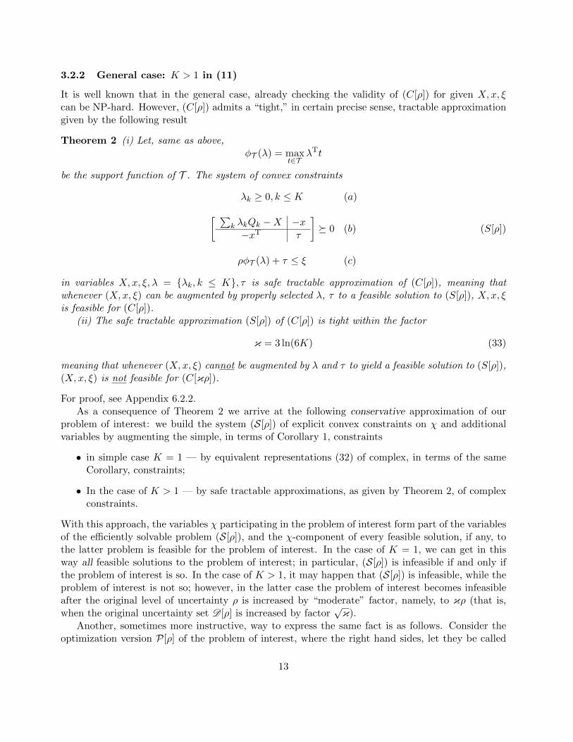
3.2.2 General case: K > 1 in (11)

It is well known that in the general case, already checking the validity of (C[ρ]) for given X,x, ξcan be NP-hard. However, (C[ρ]) admits a “tight,” in certain precise sense, tractable approximationgiven by the following result

Theorem 2 (i) Let, same as above,φT (λ) = max

t∈TλTt

be the support function of T . The system of convex constraints

λk ≥ 0, k ≤ K (a)[ ∑k λkQk −X −x−xT τ

]� 0 (b)

ρφT (λ) + τ ≤ ξ (c)

(S[ρ])

in variables X,x, ξ, λ = {λk, k ≤ K}, τ is safe tractable approximation of (C[ρ]), meaning thatwhenever (X,x, ξ) can be augmented by properly selected λ, τ to a feasible solution to (S[ρ]), X,x, ξis feasible for (C[ρ]).

(ii) The safe tractable approximation (S[ρ]) of (C[ρ]) is tight within the factor

κ = 3 ln(6K) (33)

meaning that whenever (X,x, ξ) cannot be augmented by λ and τ to yield a feasible solution to (S[ρ]),(X,x, ξ) is not feasible for (C[κρ]).

For proof, see Appendix 6.2.2.As a consequence of Theorem 2 we arrive at the following conservative approximation of our

problem of interest: we build the system (S[ρ]) of explicit convex constraints on χ and additionalvariables by augmenting the simple, in terms of Corollary 1, constraints

• in simple case K = 1 — by equivalent representations (32) of complex, in terms of the sameCorollary, constraints;

• In the case of K > 1 — by safe tractable approximations, as given by Theorem 2, of complexconstraints.

With this approach, the variables χ participating in the problem of interest form part of the variablesof the efficiently solvable problem (S[ρ]), and the χ-component of every feasible solution, if any, tothe latter problem is feasible for the problem of interest. In the case of K = 1, we can get in thisway all feasible solutions to the problem of interest; in particular, (S[ρ]) is infeasible if and only ifthe problem of interest is so. In the case of K > 1, it may happen that (S[ρ]) is infeasible, while theproblem of interest is not so; however, in the latter case the problem of interest becomes infeasibleafter the original level of uncertainty ρ is increased by “moderate” factor, namely, to κρ (that is,when the original uncertainty set D [ρ] is increased by factor

√κ).

Another, sometimes more instructive, way to express the same fact is as follows. Consider theoptimization version P[ρ] of the problem of interest, where the right hand sides, let they be called

13

γ, of the original constraints become additional to χ variables, and one seeks to minimize a givenefficiently computable convex function of γ and χ under the original constraints and, perhaps, system(A) of additional efficiently computable convex constraints on γ and χ. As is immediately seen, γ’sare among the right hand sides of the constraints of (S[ρ]), and we can apply similar procedure tothe latter system – treat γ’s as additional variables and optimize the same objective over all resultingvariables under the constraints stemming from (S[ρ]) and additional constraints (A), if any. Withthis approach, every feasible solution to the resulting optimization problem, let it be called P+[ρ],induces a feasible solution, with the same value of the objective, to P[ρ], and we have

Opt[P[ρ]] ≤ Opt[P+[ρ]] ≤ Opt[P[κρ]] ∀ρ > 0,

where Opt[P] ∈ R ∪ {+∞} stands for the optimal value of an optimization problem P.

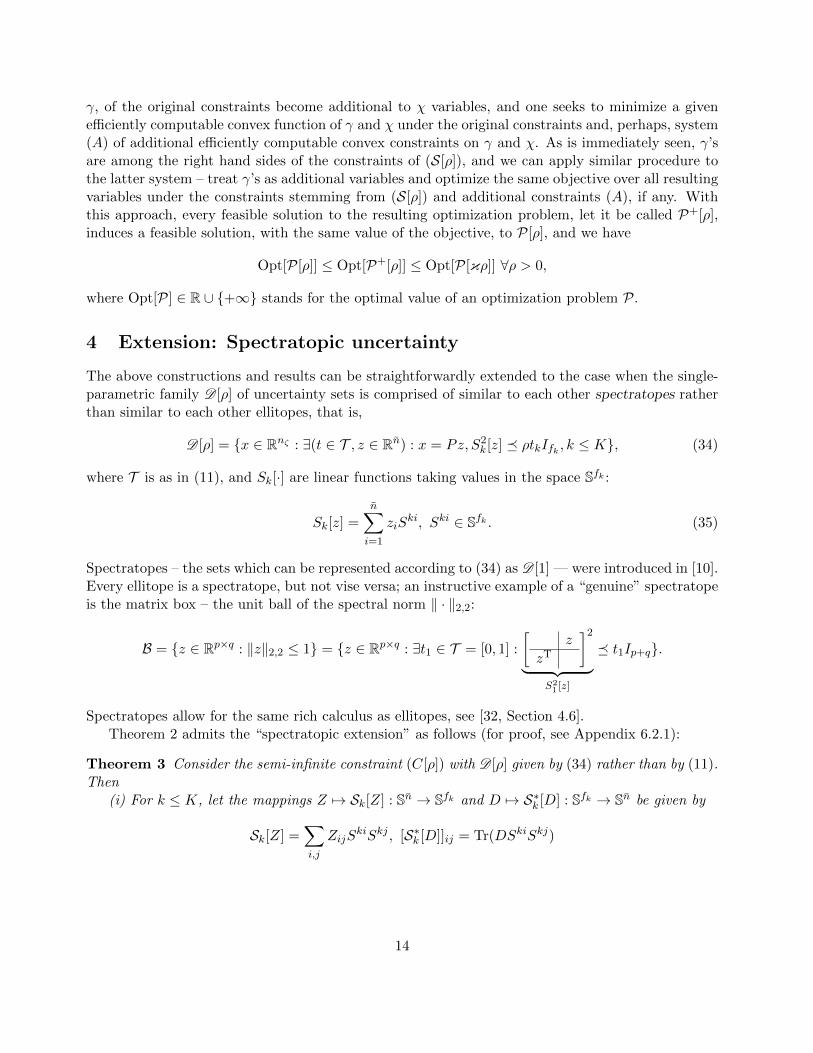
4 Extension: Spectratopic uncertainty

The above constructions and results can be straightforwardly extended to the case when the single-parametric family D [ρ] of uncertainty sets is comprised of similar to each other spectratopes ratherthan similar to each other ellitopes, that is,

D [ρ] = {x ∈ Rnζ : ∃(t ∈ T , z ∈ Rn) : x = Pz, S2k [z] � ρtkIfk , k ≤ K}, (34)

where T is as in (11), and Sk[·] are linear functions taking values in the space Sfk :

Sk[z] =

n∑i=1

ziSki, Ski ∈ Sfk . (35)

Spectratopes – the sets which can be represented according to (34) as D [1] — were introduced in [10].Every ellitope is a spectratope, but not vise versa; an instructive example of a “genuine” spectratopeis the matrix box – the unit ball of the spectral norm ‖ · ‖2,2:

B = {z ∈ Rp×q : ‖z‖2,2 ≤ 1} = {z ∈ Rp×q : ∃t1 ∈ T = [0, 1] :

[z

zT

]2

︸ ︷︷ ︸S21 [z]

� t1Ip+q}.

Spectratopes allow for the same rich calculus as ellitopes, see [32, Section 4.6].Theorem 2 admits the “spectratopic extension” as follows (for proof, see Appendix 6.2.1):

Theorem 3 Consider the semi-infinite constraint (C[ρ]) with D [ρ] given by (34) rather than by (11).Then

(i) For k ≤ K, let the mappings Z 7→ Sk[Z] : Sn → Sfk and D 7→ S∗k [D] : Sfk → Sn be given by

Sk[Z] =∑i,j

ZijSkiSkj , [S∗k [D]]ij = Tr(DSkiSkj)

14

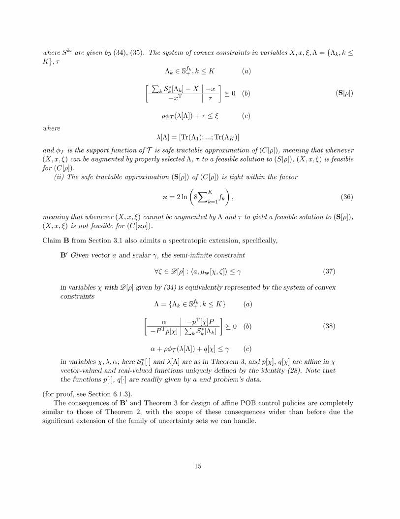
where Ski are given by (34), (35). The system of convex constraints in variables X,x, ξ,Λ = {Λk, k ≤K}, τ

Λk ∈ Sfk+ , k ≤ K (a)[ ∑k S∗k [Λk]−X −x−xT τ

]� 0 (b)

ρφT (λ[Λ]) + τ ≤ ξ (c)

(S[ρ])

whereλ[Λ] = [Tr(Λ1); ...; Tr(ΛK)]

and φT is the support function of T is safe tractable approximation of (C[ρ]), meaning that whenever(X,x, ξ) can be augmented by properly selected Λ, τ to a feasible solution to (S[ρ]), (X,x, ξ) is feasiblefor (C[ρ]).

(ii) The safe tractable approximation (S[ρ]) of (C[ρ]) is tight within the factor

κ = 2 ln

(8∑K

k=1fk

), (36)

meaning that whenever (X,x, ξ) cannot be augmented by Λ and τ to yield a feasible solution to (S[ρ]),(X,x, ξ) is not feasible for (C[κρ]).

Claim B from Section 3.1 also admits a spectratopic extension, specifically,

B′ Given vector a and scalar γ, the semi-infinite constraint

∀ζ ∈ D [ρ] : 〈a, µw[χ, ζ]〉 ≤ γ (37)

in variables χ with D [ρ] given by (34) is equivalently represented by the system of convexconstraints

Λ = {Λk ∈ Sfk+ , k ≤ K} (a)[α −pT[χ]P

−PTp[χ]∑

k S∗k [Λk]

]� 0 (b)

α+ ρφT (λ[Λ]) + q[χ] ≤ γ (c)

(38)

in variables χ, λ, α; here S∗k [·] and λ[Λ] are as in Theorem 3, and p[χ], q[χ] are affine in χvector-valued and real-valued functions uniquely defined by the identity (28). Note thatthe functions p[·], q[·] are readily given by a and problem’s data.

(for proof, see Section 6.1.3).The consequences of B′ and Theorem 3 for design of affine POB control policies are completely

similar to those of Theorem 2, with the scope of these consequences wider than before due thesignificant extension of the family of uncertainty sets we can handle.

15

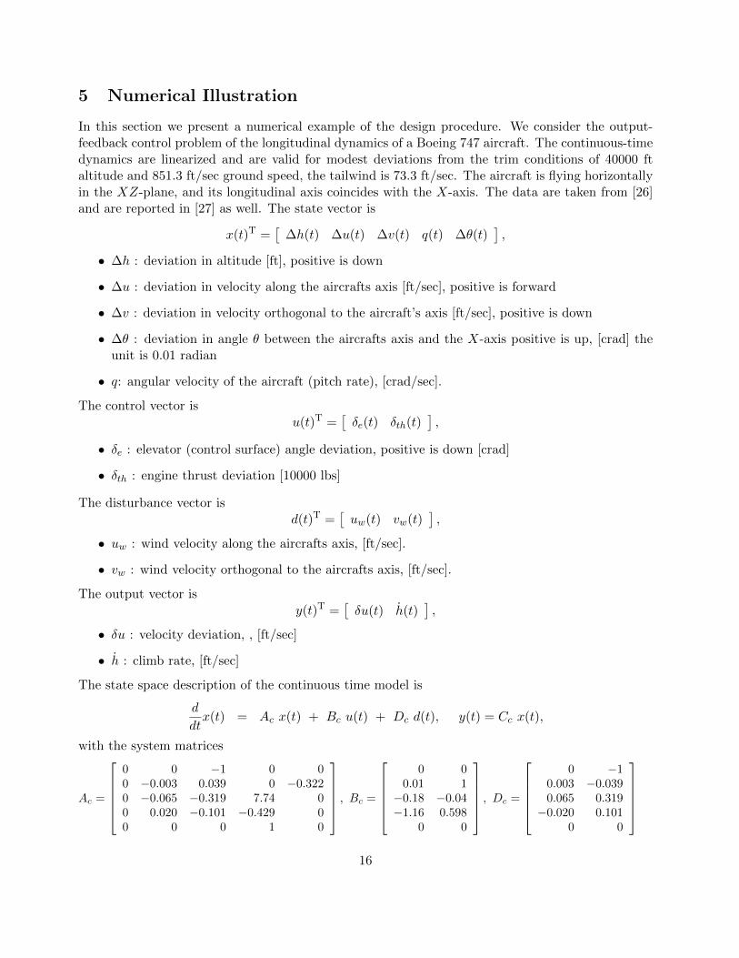
5 Numerical Illustration

In this section we present a numerical example of the design procedure. We consider the output-feedback control problem of the longitudinal dynamics of a Boeing 747 aircraft. The continuous-timedynamics are linearized and are valid for modest deviations from the trim conditions of 40000 ftaltitude and 851.3 ft/sec ground speed, the tailwind is 73.3 ft/sec. The aircraft is flying horizontallyin the XZ-plane, and its longitudinal axis coincides with the X-axis. The data are taken from [26]and are reported in [27] as well. The state vector is

x(t)T =[

∆h(t) ∆u(t) ∆v(t) q(t) ∆θ(t)],

• ∆h : deviation in altitude [ft], positive is down

• ∆u : deviation in velocity along the aircrafts axis [ft/sec], positive is forward

• ∆v : deviation in velocity orthogonal to the aircraft’s axis [ft/sec], positive is down

• ∆θ : deviation in angle θ between the aircrafts axis and the X-axis positive is up, [crad] theunit is 0.01 radian

• q: angular velocity of the aircraft (pitch rate), [crad/sec].

The control vector isu(t)T =

[δe(t) δth(t)

],

• δe : elevator (control surface) angle deviation, positive is down [crad]

• δth : engine thrust deviation [10000 lbs]

The disturbance vector isd(t)T =

[uw(t) vw(t)

],

• uw : wind velocity along the aircrafts axis, [ft/sec].

• vw : wind velocity orthogonal to the aircrafts axis, [ft/sec].

The output vector isy(t)T =

[δu(t) h(t)

],

• δu : velocity deviation, , [ft/sec]

• h : climb rate, [ft/sec]

The state space description of the continuous time model is

d

dtx(t) = Ac x(t) + Bc u(t) + Dc d(t), y(t) = Cc x(t),

with the system matrices

Ac =

0 0 −1 0 00 −0.003 0.039 0 −0.3220 −0.065 −0.319 7.74 00 0.020 −0.101 −0.429 00 0 0 1 0

, Bc =

0 0

0.01 1−0.18 −0.04−1.16 0.598

0 0

, Dc =

0 −1

0.003 −0.0390.065 0.319−0.020 0.101

0 0

16

and observation matrix

Cc =

[0 1 0 0 00 0 −1 0 7.74

].

We discretize the continuous-time dynamics at a sampling rate of T = 10 sec assuming that all the inputsignals are piecewise-constant, i.e.

u(t) ≡ uk for kT ≤ t < (k + 1)T.

The discrete-time linear time-invariant state space model is

xt+1 = A xt + B ut + B(d) (dt + et) = A xt + B ut + B(d) dt + B(s)et

yt = C xt, t = 0, 1, 2, . . . , N,

with

A = exp[AcT ], B =

∫ T

0

exp[A(T − σ)]Bcdσ, B(s) = B(d) =

∫ T

0

exp[A(T − σ)]Dcdσ, C = Cc.

The state space matrices compute to be

A =

1 −1.1267 −0.6528 −8.0749 1.58900 0.7741 0.3176 −0.9772 −2.96900 0.1157 0.0201 −0.0005 −0.36280 0.0111 0.0033 −0.0349 −0.04470 0.1388 −0.0862 0.2935 0.7579

, B =

89.1973 −50.16855.2231 6.3614−9.4731 5.9294−0.3236 0.3178−4.5318 3.2146

,

B(d) =

1.1267 −19.34720.2259 −0.3176−0.1157 0.9799−0.0111 −0.0033−0.1388 0.0862

.The linearized flight dynamics correspond to the operating conditions of 528 mph aircraft speed and50 mph steady-state tail wind. The initial state is

x0 = [0; 0; 0; 0; 0].

Our goal is to maintain the operating conditions at t = 100 sec and t = 200sec. We set the horizonat N = 20, and the target states

x10 = x20 = x0.

We assume that the stochastic noise is standard Gaussian (zero mean, unit covariance: Σ[e0;e1;...;eN−1] =I), while the deterministic disturbances satisfy the constraints

N−5∑t=0

‖dt‖22 ≤ 1,N−1∑t=N−4

‖dt‖22 ≤1

100,

reflecting the circumstance that the near horizon exogenous disturbances are more severe. Theperformance constraints are

E[‖x10 − x10‖2] ≤ 400, E[‖xN − xN‖2] ≤ 400, ΣxN � 400I

17

and are to be met robustly. We design a POB control law that meets the performance specifications.We run the computations in a MATLAB environment on a MacBook Pro with a 2.3 GHz Intel Corei5 Processor, utilizing 8 GB of RAM memory. The semidefinite program was formulated and solvedwith CVX [28], [29] using the SDPT3, [30], solver and the total computation time is less than 11seconds. The following figure depicts the altitude trajectory for 1000 realizations of the uncertainfactors, where the system evolves in accordance to the performance specifications.

18

6 Appendix

6.1 Justifying claims in Section 3.1

6.1.1 Justifying claim A

In the notation of item A and setting Z = D [ρ], we should prove that χ satisfies (22), or, which isthe same by (21), the constraint

∀(ζ ∈ Z) : [ζ; 1]TZT[χ]AZ[χ][ζ; 1]− 2βTAZ[χ][ζ; 1] + Tr(Π1/2ET[χ]AE[χ]Π1/2) + r ≤ γ, (39)

if and only if χ can be augmented to the feasible solution to (23).1) Assume that χ satisfies (39), and let us define X,x, α, δ according to[

X x

xT α

]= ZT[χ]AZ[χ] (a)

δ = maxz∈Z

[zTXz + 2xTz − 2βTAZ[χ][z; 1]

](b)

(a) ensures the validity of (23.a), and (a, b) together with (39) ensure the validity (23.b). Finally,identity (24) and (b) say that

δ = maxz∈Z

[zTXz + 2[x+ p[χ]]Tz + q[χ]

],

implying the validity of (23.c)2) Now assume that χ,X, x, α, δ satisfy (23). Then

δ ≥ maxz∈Z

[zTXz + 2xTz − 2βTAZ[χ][z; 1]

]by (23.c) combined with (24), whence

maxz∈Z

[[z; 1]T

[X x

xT α

][z; 1]− 2βTAZ[χ][z; 1]

]≤ δ + α,

which combines with (23.a) to imply that

maxz∈Z

[[z; 1]TZT[χ]AZ[χ][z; 1]− 2βTAZ[χ][z; 1]

]≤ δ + α.

The resulting inequality combines with (23.b) to imply the validity of (39). �

6.1.2 Justifying claim B

In view of (28) and (11), constraint (26) reads

γ − q[χ] ≥ Opt[χ] := maxz∈D [ρ]

2zTp[χ] = maxy,t

{2yTPTp[χ] : yTSky ≤ ρtk, k ≤ K, t ∈ T

}.

19

Optimization problem specifying Opt[χ] clearly is convex, bounded and satisfies Slater condition.Applying Lagrange Duality Theorem, we get the first equivalence in the following chain:

γ − q[χ] ≥ Opt[χ]

⇔ ∃λ ≥ 0 : γ − q[χ] ≥ supt∈T ,y

{2yTPTp[χ]−

∑k

λk(yTSky − ρtk)

}︸ ︷︷ ︸

=ρφT (λ)+supy{2yTPTp[χ]−yT[∑k λkSk]y}

⇔ ∃λ ≥ 0, α : γ − q[χ] ≥ ρφT + α &

[α −pT[χ]P

−PTp[χ]∑

k λkSk

]� 0,

and B follows. �

6.1.3 Justifying claim B′

Preliminaries. We start with the well-known “conic extension” of Lagrange Duality Theorem:

Theorem 4 Let K be regular (i.e., closed convex pointed and with a nonempty interior) cone in someEuclidean space E, K∗ be the cone dual to K, let W be a convex set in some Rn, let f(w) : W → R beconvex, and let g(w) : W → Ek be K-convex, meaning that λg(u)+(1−λ)g(v)−g(λu+(1−λ)v) ∈ Kfor all u, v ∈W and λ ∈ [0, 1]. Consider the feasible convex optimization problem

Opt(P ) = minw{f(w) : g(w) ≤K 0, w ∈W} , (P )

where a ≥K b (⇔ b ≤K a) means that a − b ∈ K. Along with (P ), consider its “conic” Lagrangefunction

L(w,Λ) = f(w) + 〈Λ, g(w)〉 : W ×K∗ → R

and “conic” Lagrange dual

Opt(D) = maxΛ

{f∗(Λ) := inf

w∈WL(w, λ),Λ ∈ K∗

}. (D)

Then Opt(D) ≤ Opt(P ). Moreover, assuming that (P ) is bounded and satisfies Slater condition:

−g(w) ∈ intK

for some w ∈W , (D) is solvable and Opt(P ) = Opt(D).

Note that the standard Lagrange Duality Theorem is the special case of Theorem 4 correspondingto the case when K is the nonnegative orthant in some Rn.

To make the paper self-contained, here is the proof of Theorem 4. First, it is immediately seenthat when Λ ∈ K∗, L(w,Λ) underestimates f(w) on the feasible set of (P ), whence f∗(Λ) ≤ Opt(P )on the feasible domain of (D), implying that Opt(D) ≤ Opt(P ). Now assume that (P ) is boundedand satisfies Slater condition, and let

S = {(τ, x) ∈ R× E : τ < Opt(P ), x ≤K 0}, T = {(τ, x) ∈ R× E : ∃w ∈W : f(w) ≤ τ, g(w) ≤K x}.

20

It is immediately seen that S and T are nonempty nonintersecting convex sets, implying that thereexists a nonzero (α,M) ∈ R× E such that

sup(τ,x)∈S

[ατ + 〈x,M〉] ≤ inf(τ,x)∈T

[ατ + 〈x,M〉] . (40)

By this relation, the right hand side quantity is finite, and since R+ ×K clearly is contained in therecessive cone of T , we conclude that α > 0 and M ∈ K∗. As a result, by construction of S, T (40)reads

αOpt(P ) ≤ infw∈W

[αf(w) + 〈M, g(w)〉] . (41)

When α > 0, setting Λ = M/α, we get Λ ∈ K∗, and (41) says that f∗(Λ) ≥ Opt(P ); since, as we haveseen, Opt(D) ≤ Opt(P ), we conclude that Λ is an optimal solution to (D) and Opt(P ) = Opt(D).

It remains to verify that we indeed have α > 0. Assuming this is not the case, α = 0, and (41)combines with w ∈W to imply that 〈g(w),M〉 ≥ 0. Since −g(w) ∈ intK and M ∈ K∗, we concludethat M = 0, whence (α,M) = 0, which is not the case. �

Theorem 4⇒ B′: In view of (28) and (34), constraint (37) reads

γ−q[χ] ≥ maxz∈D [ρ]

2zTp[χ] = −Opt[χ], Opt[χ] = miny,t

{−2yTPTp[χ] : S2

k [y]− ρtkIfk � 0, k ≤ K, t ∈ T}.

Setting E = Sf1 × ... × SfK , K = Sf1+ × ... × SfK+ , g(y) = Diag{S21 [y] − ρt1If1 , ..., S2

K [y] − ρtKIfK},(37) becomes

γ − q[χ] ≥ −Opt[χ], Opt[χ] = minw∈W{f(y) := −2yTPTp[χ] : g(y) ≤K 0

},

W = {(y, t) : t ∈ T }. (42)

The problem specifying Opt[χ] is of the form (P ) considered in Theorem 4 and clearly is belowbounded and satisfies Slater condition. Applying Theorem 4 and noting that, as is immediatelyseen, Tr(S2

k [y]Λk) = yTS∗k [Λk]y, we conclude that

−Opt[χ]

= −maxΛ

{f∗(Λ) := inf

t∈T ,y

[−2yTPTp[χ] + yT [

∑k S∗k [Λk]] y − ρ

∑k Tr[Λk]tk : Λ = {Λk ∈ Sfk+ , k ≤ K}

]}= −max

Λ

{infy

[−2yTPTp[χ] + yT [

∑k S∗k [Λk]] y

]− ρφT (λ[Λ]) : Λ = {Λk ∈ Sfk+ , k ≤ K}

}= min

Λ

{ρφT (λ[Λ]) + sup

y

[2yTPTp[χ]− yT [

∑k S∗k [Λk]] y

]: Λ = {Λk ∈ Sfk+ , k ≤ K}

}= min

Λ,α

{ρφT (λ[Λ]) + α :

[α −pT[χ]P

−PTp[χ]∑k S∗k [Λk]

]� 0,Λ = {Λk ∈ Sfk+ , k ≤ K}

}and the maxima, and therefore the minima, in the right hand side are achieved. This conclusioncombines with (42) to imply B′. �

6.2 Proofs of Theorems 2, 3

Theorems 2, 3 are essential extensions of the results of [31] where, in retrospect, a special ellitope –intersection of concentric ellipsoids – was considered;

21

6.2.1 Proof of Theorem 3

00. By replacing T with ρT , we can reduce the situation to the one where ρ = 1, which is assumedfrom now on.

10 For s > 0, let

X [s] = {x ∈ Rn : ∃z ∈ Z[s] :={z ∈ RN : ∃t ∈ T : S2

k[z] ≤ stkIfk , k ≤ K}

: x = Pz},Sk[z] =

∑i ziS

ki, Ski ∈ Sfk

be a single-parametric family of spectratopes. Let also

F (x) = xTAx+ 2bTx, Opt∗[s] = maxx{F (x) : x ∈ X [s]} .

Note that

Opt∗[s] = maxz

{G(z) = zTQz + 2qTz : z ∈ Z[s]

}, Q = PTAP, q = PTb.

Let us set

Q+ =

[Q q

qT

].

For Λ = {Λk ∈ Sfk , k ≤ K}, let

λ[Λ] = [Tr(Λ1); ...; Tr(ΛK)],Sk[Q] =

∑i,j QijS

kiSkj =∑

i,j Qij12 [SkiSkj + SkjSki] : SN → Sfk

S∗k [Λk] =[Tr(ΛkS

kiSkj)]i.j

=[Tr(Λk

12 [SkiSkj + SkjSki])

]i,j

: Sfk → SN .

Note that the mappings Sk, S∗k are conjugate to each other:

Tr(Sk[Q]Λk) = Tr(QS∗k [Λk]), Q ∈ SN ,Λk ∈ Sfk

20. Our local goal is to prove the following

Proposition 5 Let

Opt[s] = minΛ,µ

sφT (λ[Λ]) + µ :

Λ = {Λk � 0, k ≤ K}, µ ≥ 0

Q+ �[ ∑

k S∗k [Λk]

µ

] . (43)

ThenOpt∗[s] ≤ Opt[s] ≤ Opt∗[κs] (44)

with

κ = 2 ln

(8

K∑k=1

fk

). (45)

22

Proof of Proposition. Replacing T with sT , we can assume once for ever that s = 1. Now, setting

T = cl{[t; τ ] : τ > 0, t/τ ∈ T }

we get a closed convex pointed cone with a nonempty interior, the dual cone being

T∗ = {[g; s] : s ≥ φT (−g)}.

Problem (43) with s = 1 is the conic problem

Opt[1] = minΛ,τ,µ

τ + µ :

Λk � 0, k ≤ K,µ ≥ 0[−λ[Λ]; τ ] ∈ T∗[ ∑

k S∗k [Λk]

µ

]−Q+ � 0

. (∗)

It is immediately seen that this problem is strictly feasible and solvable, so that Opt[1] is the optimalvalue in the conic dual of (∗). To get the latter problem, let Pk � 0, p ≥ 0, [t; s] ∈ T, and

W =

[V vvT w

]� 0 be Lagrange multipliers for the respective constraints in (∗). Aggregating the

constraints with these weights, we get∑k

Tr(PkΛk) + pµ− tTλ[Λ] + τs+ Tr(V∑k

S∗k [Λk])− Tr(V Q)− 2vTq + wµ ≥ 0,

that is, ∑k

Tr([Pk + Sk[V ]− tkIdk ]ΛK) + [p+ w]µ+ τs ≥ Tr(V Q) + 2vTq.

To get the dual problem, we add to the above restrictions on the Lagrange multipliers the requirementthat the left hand side in the latter inequality, identically in Λk, τ , and µ should be equal to theobjective in (∗), implying, in particular, that t ∈ T , s = 1, and w ≤ 1. We see that the dual problem,after evident simplifications, becomes

Opt[1] = maxV,v,t

Tr(V Q) + 2vTq :

t ∈ T , Sk[V ] � tkIfk , k ≤ K,[V v

vT 1

]� 0.

(46)

By definition,Opt∗[1] = max

z,t

{zTQz + 2qTz : t ∈ T , S2

k [z] � tkIfk , k ≤ K}.

If (z, t) is a feasible solution to the latter problem, then V = zzT, v = z, t is a feasible solution to (46)with the same value of the objective, implying that Opt[1] ≥ Opt∗[1], as stated in the first relationin (44) (recall that we are in the case of s = 1).

We have already stated that problem (46) is solvable. Let V∗, v∗, t∗ be its optimal solution, and

let

X =

[V∗ v∗vT∗ 1

].

23

Let χ be Rademacher random vector3 of the same size as the one of Q+, let

X1/2Q+X1/2 = UDiag{λ}UT

with orthogonal U , and let ζ = X1/2Uχ = [ξ; τ ], where τ is the last entry in ζ. Then

ζTQ+ζ = χTUTX1/2Q+X1/2Uχ = χTDiag{λ}χ

=∑

i λi = Tr(X1/2Q+X1/2) = Tr(XQ+) = Opt[1].

(47)

Next, we have

ζζT =

[ξξT τξ

τξT τ2

]= X1/2UχχTUTX1/2,

whence

E{ζζT} =

[E{ξξT} E{τξ}E{τξT} E{τ2}

]= X =

[V∗ v∗vT∗ 1

]. (48)

In particular,Sk[E{ξξT}] = Sk[V∗] � t∗kIfk , k ≤ K.

We have ξ = Wχ for certain rectangular matrix W such that V∗ = E{ξξT} = E{ WχχTWT} =WWT. Consequently,

Sk[ξ] = Sk[Wχ] =∑i

χiSki := Sk[χ]

with some symmetric matrices Ski. As a result,

Sk[ξξT] = S2k [ξ] =

∑i,j

χiχjSkiSkj ,

and taking expectation we get∑i

[Ski]2 = Sk[E{ξξT}] = Sk[V∗] � t∗kIfk ,

whence by Noncommutative Khintchine Inequality (see, e.g., [32, Theorem 4.45]) one has

Pr{S2k [ξ] � t∗kr−1Ifk} = Pr{S2

k [χ] � t∗kr−1Ifk} ≤ 1− 2fk exp{− 1

2r}, 0 < r ≤ 1. (49)

Next, invoking (48) we haveE{τ2} = E{[ζζT]N+1,N+1} = 1 (50)

andτ = βTχ

for some vector β with ‖β‖2 = 1 due to (50). Now let us invoke the following fact [31, Lemma A.1]

Lemma 6 Let β be a deterministic ‖ · ‖2-unit vector in RN and χ be N -dimensional Rademacherrandom vector. Then Pr{|βTχ| ≤ 1} ≥ 1/3.

3random vector with independent entries taking values ±1 with probabilities 1/2.

24

Now let r be given by the relation

r =1

2 ln(8∑

k fk),

implying that

2

K∑k=1

fk exp{− 1

2r} < 1/3.

By (49) and Lemma 6 there exists a realization ζ = [ξ; τ ] of ζ such that

S2k [ξ] � t∗kr−1Ifk , k ≤ K, & |τ | ≤ 1. (51)

Invoking (47) and taking into account that |τ | ≤ 1 we have

Opt[1] = ζTQ+ζ = ξTQξ + 2τ qTξ ≤ ξTQξ + 2qTξ,

where ξ = ξ when qTξ ≥ 0 and ξ = −ξ otherwise. In both cases from the first relation in (51) weconclude that ξ ∈ Z[1/r], and we arrive at Opt[1] ≤ Opt∗[2 ln(8

∑k fk)]. Proposition 5 is proved.

30. We are ready to complete the proof of Theorem3. Indeed, by replacing T with ρT , we reducethe situation considered in Theorem to the one where ρ = 1. Now, using the notation from Theorem,let us set

n = nζ , N = n, Q+ =

[X x

xT

].

thus ensuring that X [1] = D [1]. Q∗, K and the entities participating in Theorem 3 give rise to thedata participating in Proposition 5. In terms of this Proposition, the fact that X,x, ξ is feasible for(C[s]) with s > 0 is nothing but the relation

Opt∗[s] ≤ ξ,

and the fact that X,x, ξ can be extended by properly selected Λ, τ to a feasible solution to (S[s]) isexactly the relation

Opt[s] ≤ ξ.

As a result, Theorem 3 becomes an immediate consequence of Proposition 5, with item (i) of Theoremreadily given by the left, and item (ii) – by the right inequality in (44).

6.2.2 Proof of Theorem 2

10. Consider a single-parametric family of ellitopes

X [s] = {x : ∃z ∈ Z[s] : x = Pz}, Z[s] = {z ∈ RN : ∃t ∈ T : zTSkz ≤ stk, k ≤ K} , s > 0. (52)

Let alsoF (x) = xTAx+ 2bTx, Opt∗[s] = max

x{F (x) : x ∈ X [s]} /

Note that

Opt∗[s] = maxz

{G(z) = zTQz + 2qTz : z ∈ Z[s]

}, Q = PTAP, q = PTb.

25

Let us set

Q+ =

[Q q

qT

].

The ellitopic version of Proposition 5 reads as follows:

Proposition 7 Let

Opt[s] = minλ,µ

sφT (λ) + µ :

λ = {λk ≥ 0, k ≤ K}, µ ≥ 0

Q+ �[ ∑

k S∗k [Λk]

µ

] . (53)

ThenOpt∗[s] ≤ Opt[s] ≤ Opt∗[κs] (54)

withκ = 3 ln(6K). (55)

Theorem 2 can be immediately derived from this Proposition in exactly the same fashion as Theorem3 above was derived from Proposition 5.

30. Proof of Proposition 7 is similar to the one of Proposition 5. Specifically,

30.1. We have

Opt∗[s] = maxz,t

{zTQz + 2qTz : t ∈ T , zTSkz ≤ stk, k ≤ K

},

and

Opt[s] = minλ,µ

sφT (λ) + µ :

λ ≥ 0, µ ≥ 0[ ∑k λkSk

µ

]−Q+ � 0

= minλ,µ,τ

sτ + µ :

λ ≥ 0, µ ≥ 0, [−λ; τ ] ∈ T∗[ ∑k λkSk

µ

]−Q+ � 0

.

30.2. Same as in the spectratopic case, it suffices to consider the case when s = 1, which is assumedfrom now on.

The problem dual to the conic problem specifying Opt[1] reads

Opt[1] = maxV,v,t

Tr(QV ) + 2qTv :

t ∈ T ,Tr(SkV ) ≤ tk, k ≤ K[V v

vT 1

]� 0

(56)

Every feasible solution (z, t) to the problem specifying Opt∗[1] gives rise to the feasible solution(V = zzT, v = z, t) to (56) with the same value of the objective, implying that Opt∗[1] ≤ Opt[1]

26

30.3. It is easily seen that (56) has an optimal solution V∗, v∗, t∗. Setting

X =

[V∗ v∗vT∗ 1

],

we setX1/2Q+X

1/2 = Udiag{λ}UT

with orthogonal U , setζ = X1/2Uχ

with Rademacher random χ, thus ensuring that

ζTQ+ζ = χTUTX1/2Q+X1/2Uχ = χTdiag{λ}χ =

∑i

λi = Tr(XQ+) = Opt[1]. (57)

At the same time, setting ζ = [ξ; τ ] with scalar τ , we get[E{ξξT} E{τξ}E{τξT} E{τ2}

]= E{ζζT} = E{X1/2UχχTUTX1/2} = X =

[V∗ v∗vT∗ 1

].

As before, we have ξ = Wχ for some deterministic matrix W , and E{ξTSkξ} = Tr(SkV∗) ≤ t∗k,whence Tr(WTSkW ) = E{χTWTSkWχ} = E{ξTSkξ} ≤ t∗k. By [32, Lemma 4.28] the relationsWTSkW � 0, Tr(WTSkW ) ≤ t∗k imply that

Pr{ξTSkξ > γt∗k} = Pr{χTWTSkWχ > γt∗k} ≤√

3 exp{−γ3}, ∀γ > 0,

(cf. the proof of [32, Proposition 4.6]).

30.4. Now the reasoning completely similar to the one in the spectratopic case shows that whenκ = 3 ln(6K), there exists a realization ζ = [ξ; τ ] of ζ such that S2

k [ξ] ≤ t∗kκ for all k and |τ | ≤ 1.This conclusion, taken together with (57), results in Opt[1] ≤ Opt∗[κ], thus completing the proof.

Acknowledgment

The authors gratefully acknowledge the support of National Science Foundation grants 1637473,1637474, and the NIFA grant 2020-67021-31526.

References

[1] Y. Chen, T. T. Georgiou, M. Pavon, Optimal Steering of a Linear Stochastic System to a FinalProbability Distribution, Part I. IEEE Trans. on Automatic Control 61(5):1158-1169, 2016

[2] Y. Chen, T. T. Georgiou, M. Pavon, Optimal Steering of a Linear Stochastic System to a FinalProbability Distribution, Part II. IEEE Trans. on Automatic Control 61(5):1170–1180, 2016

[3] Y. Chen, T. T. Georgiou, M. Pavon, Optimal Steering of a Linear Stochastic System to a FinalProbability Distribution, Part III. IEEE Trans. on Automatic Control 63(9):3112-3118, 2016

27

[4] E. Bakolas, Finite-horizon covariance control for discrete-time stochastic linear systems subjectto input constraints. Automatica 91:61–68, 2018.

[5] K. Okamoto, M. Goldshtein, P. Tsiotras, Optimal Covariance Control for Stochastic SystemsUnder Chance Constraints. IEEE Control Systems Letters 2(2):266-271, 2018.

[6] A. Juditsky, A. Nemirovski, Near-optimality of linear recovery in Gaussian observation schemeunder ‖ · ‖22 loss. Ann. of Statist. 46(4):1603-1629, 2018.

[7] K. Zhou, J. C. Doyle, K. Glover Robust and Optimal Control Prentice Hall, Upper Saddle River,NJ, 1996.

[8] T. Basar, P. Bernhard, H∞-Optimal Control and Related Minimax Design Problems Birkhauser,Boston, MA, 1995.

[9] I. Petersen, V. A. Ugrinovskii, A. V. Savkin, Robust Control Design Using H∞ Methods Springer-Verlag London 2000.

[10] A. Juditsky, A. Nemirovski, Near-Optimality of Linear Recovery from Indirect Observations.Mathematical Statistics and Learning 1:2 (2018), 171-225.

[11] A. F. Hotz, R. E. Skelton, A covariance control theory. 24th IEEE Conference on Decision andControl Fort Lauderdale, FL, USA, 552–557, 1985.

[12] A. F. Hotz, R. E. Skelton, Covariance control theory. International Journal of Control 46(1)13-32, 1987.

[13] R.E. Skelton, T. Iwasaki, K. Grigoriadis, A Unified Algebraic Approach to Linear Control DesignTaylor & Francis, London, UK, 1998

[14] D. Youla, J. Bongiorno and H. Jabr, Modern Wiener–Hopf design of optimal controllers Part I:The single-input-output case, IEEE Trans. on Automatic Control 21(1):3-13, 1976

[15] D. Youla, J. Bongiorno and H. Jabr, Modern Wiener–Hopf design of optimal controllers PartII: The multivariable case, IEEE Trans. on Automatic Control 21(3):319-338, 1976

[16] A. Ben-Tal, S. Boyd, A. Nemirovski, Extending scope of robust optimization: Comprehensiverobust counterparts of uncertain problems. Math. Programming Ser. B 107: 63–89, 2006

[17] D. Bertsimas, D. A. Iancu, P.A. Parrilo, Optimality of affine policies in multistage robust opti-mization. Math. of Oper. Res. 35(2): 363–394, 2010.

[18] D. Bertsimas, D. A. Iancu, P.A. Parrilo, A hierarchy of near-optimal policies for multistageadaptive optimization. IEEE Trans. Automatic Control 56(12):2809–2823, 2009.

[19] D. Kuhn, W. Wiesemann, A. Georghiou, Primal and dual linear decision rules in stochastic androbust optimization. Math. Programming 130(1): 177–209, 2011.

[20] X. Chen, M. Sim, P. Sun, J. Zhang, A linear decision-based approximation approach to stochasticprogramming. Oper. Res. 56(2):344–357, 2008.

28

[21] A. Nemirovski, A. Shapiro, On complexity of stochastic programming problems. ContinuousOptimization: Current Trends and Applications Springer-Verlag, New York, NY 111–146, 2005

[22] J. Lofberg, Approximations of closed-loop MPC. Proceedings of the 42nd IEEE Conf. on Deci-sion and Control 1438–1442, 2003.

[23] P. J. Goulart, E. C. Kerrigan, J. M. Maciejowski, Optimization over state feedback policies forrobust control with constraints. Automatica 42: 523–533, 2006.

[24] P. J. Goulart, E. C. Kerrigan, Output feedback receding horizon control of constrained systems.International Journal of Control 80: 8–20, 2007.

[25] J. Skaf, S. Boyd, Design of affine controllers via convex optimization. IEEE Trans. on AutomaticControl 55(11): 2476–2487, 2010.

[26] Stephen Boyd’s EE263 Lecture Noteshttps://web.stanford.edu/class/archive/ee/ee263/ee263.1082/lectures/aircraft2.pdf

[27] A. Ben-Tal, A. Nemirovski, Lectures on Modern Convex Optimization: Analysis, Algorithms,Engineering Applications SIAM, Philadelphia, PA, 2019.

[28] M. Grant, S. Boyd, CVX: MATLAB Software for Disciplined Convex Programming, Version2.1, 2014

[29] M. Grant, S. Boyd, Y. Ye, Disciplined Convex Programming. In L Liberti, N Maculan (eds.),Global Optimization: From Theory to Implementation, Nonconvex Optimization and its Appli-cations, pp. 155–210. Springer, 2006.

[30] K. C. Toh, M. J. Todd, R. H. Tutuncu, SDPT3 — a Matlab software package for semidefiniteprogramming, Optimization Methods and Software, 11: 545–581, 1999.

[31] Ben-Tal, A. Nemirovski, C. Roos, Robust solutions to uncertain quadratic and conic-quadraticproblems. SIAM J. on Optimization 13:2 , 535–560, 2002.

[32] A. Juditsky, A. Nemirovski, Statistical Inference via Convex Optimization Princeton UniversityPress, April 2020

29