CONVEX ANALYSIS AND NONLINEAR … ANALYSIS AND NONLINEAR OPTIMIZATION Theory and Examples Second...
317
CONVEX ANALYSIS AND NONLINEAR OPTIMIZATION Theory and Examples Second Edition JONATHAN M. BORWEIN Faculty of Computer Science Dalhousie University, Halifax, NS, Canada B3H 2Z6 [email protected] http://users.cs.dal.ca/∼jborwein and ADRIAN S. LEWIS School of Operations Research and Industrial Engineering Cornell University [email protected] http://www.orie.cornell.edu/∼aslewis
-
Upload
trinhquynh -
Category
Documents
-
view
220 -
download
1
Transcript of CONVEX ANALYSIS AND NONLINEAR … ANALYSIS AND NONLINEAR OPTIMIZATION Theory and Examples Second...
CONVEX ANALYSIS AND NONLINEAR
OPTIMIZATION
Theory and Examples
Second Edition
JONATHAN M. BORWEINFaculty of Computer Science
Dalhousie University, Halifax, NS, Canada B3H [email protected]
http://users.cs.dal.ca/∼jborwein
and
ADRIAN S. LEWISSchool of Operations Research and Industrial Engineering
Cornell [email protected]
http://www.orie.cornell.edu/∼aslewis

To our families
v

vi
Preface
Optimization is a rich and thriving mathematical discipline. Propertiesof minimizers and maximizers of functions rely intimately on a wealth oftechniques from mathematical analysis, including tools from calculus andits generalizations, topological notions, and more geometric ideas. Thetheory underlying current computational optimization techniques growsever more sophisticated—duality-based algorithms, interior point methods,and control-theoretic applications are typical examples. The powerful andelegant language of convex analysis unifies much of this theory. Henceour aim of writing a concise, accessible account of convex analysis and itsapplications and extensions, for a broad audience.
For students of optimization and analysis, there is great benefit to blur-ring the distinction between the two disciplines. Many important analyticproblems have illuminating optimization formulations and hence can be ap-proached through our main variational tools: subgradients and optimalityconditions, the many guises of duality, metric regularity and so forth. Moregenerally, the idea of convexity is central to the transition from classicalanalysis to various branches of modern analysis: from linear to nonlinearanalysis, from smooth to nonsmooth, and from the study of functions tomultifunctions. Thus, although we use certain optimization models re-peatedly to illustrate the main results (models such as linear and semidefi-nite programming duality and cone polarity), we constantly emphasize thepower of abstract models and notation.
Good reference works on finite-dimensional convex analysis already ex-ist. Rockafellar’s classic Convex Analysis [167] has been indispensable andubiquitous since the 1970s, and a more general sequel with Wets, Varia-tional Analysis [168], appeared recently. Hiriart–Urruty and Lemarechal’sConvex Analysis and Minimization Algorithms [97] is a comprehensive butgentler introduction. Our goal is not to supplant these works, but on thecontrary to promote them, and thereby to motivate future researchers. Thisbook aims to make converts.
vii
viii Preface
We try to be succinct rather than systematic, avoiding becoming boggeddown in technical details. Our style is relatively informal; for example, thetext of each section creates the context for many of the result statements.We value the variety of independent, self-contained approaches over a sin-gle, unified, sequential development. We hope to showcase a few memorableprinciples rather than to develop the theory to its limits. We discuss noalgorithms. We point out a few important references as we go, but we makeno attempt at comprehensive historical surveys.
Optimization in infinite dimensions lies beyond our immediate scope.This is for reasons of space and accessibility rather than history or appli-cation: convex analysis developed historically from the calculus of vari-ations, and has important applications in optimal control, mathematicaleconomics, and other areas of infinite-dimensional optimization. However,rather like Halmos’s Finite Dimensional Vector Spaces [90], ease of ex-tension beyond finite dimensions substantially motivates our choice of ap-proach. Where possible, we have chosen a proof technique permitting thosereaders familiar with functional analysis to discover for themselves how aresult extends. We would, in part, like this book to be an entree for math-ematicians to a valuable and intrinsic part of modern analysis. The finalchapter illustrates some of the challenges arising in infinite dimensions.
This book can (and does) serve as a teaching text, at roughly the levelof first year graduate students. In principle we assume no knowledge of realanalysis, although in practice we expect a certain mathematical maturity.While the main body of the text is self-contained, each section concludeswith an often extensive set of optional exercises. These exercises fall intothree categories, marked with zero, one, or two asterisks, respectively, asfollows: examples that illustrate the ideas in the text or easy expansionsof sketched proofs; important pieces of additional theory or more testingexamples; longer, harder examples or peripheral theory.
We are grateful to the Natural Sciences and Engineering Research Coun-cil of Canada for their support during this project. Many people havehelped improve the presentation of this material. We would like to thank allof them, but in particular Patrick Combettes, Guillaume Haberer, ClaudeLemarechal, Olivier Ley, Yves Lucet, Hristo Sendov, Mike Todd, XianfuWang, and especially Heinz Bauschke.
Jonathan M. BorweinAdrian S. Lewis
Gargnano, ItalySeptember 1999

Preface ix
Preface to the Second Edition
Since the publication of the First Edition of this book, convex analysisand nonlinear optimization has continued to flourish. The “interior pointrevolution” in algorithms for convex optimization, fired by Nesterov andNemirovski’s seminal 1994 work [148], and the growing interplay betweenconvex optimization and engineering exemplified by Boyd and Vanden-berghe’s recent monograph [47], have fuelled a renaissance of interest in thefundamentals of convex analysis. At the same time, the broad success ofkey monographs on general variational analysis by Clarke, Ledyaev, Sternand Wolenski [56] and Rockafellar and Wets [168] over the last decade tes-tify to a ripening interest in nonconvex techniques, as does the appearanceof [43].
The Second Edition both corrects a few vagaries in the original andcontains a new chapter emphasizing the rich applicability of variationalanalysis to concrete examples. After a new sequence of exercises endingChapter 8 with a concise approach to monotone operator theory via convexanalysis, the new Chapter 9 begins with a presentation of Rademacher’sfundamental theorem on differentiability of Lipschitz functions. The sub-sequent sections describe the appealing geometry of proximal normals, fourapproaches to the convexity of Chebyshev sets, and two rich concrete mod-els of nonsmoothness known as “amenability” and “partial smoothness”.As in the First Edition, we develop and illustrate the material throughextensive exercises.
Convex analysis has maintained a Canadian thread ever since Fenchel’soriginal 1949 work on the subject in Volume 1 of the Canadian Journalof Mathematics [76]. We are grateful to the continuing support of theCanadian academic community in this project, and in particular to theCanadian Mathematical Society, for their sponsorship of this book series,and to the Canadian Natural Sciences and Engineering Research Councilfor their support of our research endeavours.
Jonathan M. BorweinAdrian S. Lewis
September 2005
Contents
Preface vii
1 Background 11.1 Euclidean Spaces . . . . . . . . . . . . . . . . . . . . . . . . 11.2 Symmetric Matrices . . . . . . . . . . . . . . . . . . . . . . 9
2 Inequality Constraints 152.1 Optimality Conditions . . . . . . . . . . . . . . . . . . . . . 152.2 Theorems of the Alternative . . . . . . . . . . . . . . . . . . 232.3 Max-functions . . . . . . . . . . . . . . . . . . . . . . . . . . 28
3 Fenchel Duality 333.1 Subgradients and Convex Functions . . . . . . . . . . . . . 333.2 The Value Function . . . . . . . . . . . . . . . . . . . . . . 433.3 The Fenchel Conjugate . . . . . . . . . . . . . . . . . . . . . 49
4 Convex Analysis 654.1 Continuity of Convex Functions . . . . . . . . . . . . . . . . 654.2 Fenchel Biconjugation . . . . . . . . . . . . . . . . . . . . . 764.3 Lagrangian Duality . . . . . . . . . . . . . . . . . . . . . . . 88
5 Special Cases 975.1 Polyhedral Convex Sets and Functions . . . . . . . . . . . . 975.2 Functions of Eigenvalues . . . . . . . . . . . . . . . . . . . . 1045.3 Duality for Linear and Semidefinite Programming . . . . . . 1095.4 Convex Process Duality . . . . . . . . . . . . . . . . . . . . 114
6 Nonsmooth Optimization 1236.1 Generalized Derivatives . . . . . . . . . . . . . . . . . . . . 1236.2 Regularity and Strict Differentiability . . . . . . . . . . . . 1306.3 Tangent Cones . . . . . . . . . . . . . . . . . . . . . . . . . 1376.4 The Limiting Subdifferential . . . . . . . . . . . . . . . . . . 145
x
Contents xi
7 Karush–Kuhn–Tucker Theory 1537.1 An Introduction to Metric Regularity . . . . . . . . . . . . 1537.2 The Karush–Kuhn–Tucker Theorem . . . . . . . . . . . . . 1607.3 Metric Regularity and the Limiting Subdifferential . . . . . 1667.4 Second Order Conditions . . . . . . . . . . . . . . . . . . . 172
8 Fixed Points 1798.1 The Brouwer Fixed Point Theorem . . . . . . . . . . . . . . 1798.2 Selection and the Kakutani–Fan Fixed Point Theorem . . . 1908.3 Variational Inequalities . . . . . . . . . . . . . . . . . . . . . 200
9 More Nonsmooth Structure 2139.1 Rademacher’s Theorem . . . . . . . . . . . . . . . . . . . . 2139.2 Proximal Normals and Chebyshev Sets . . . . . . . . . . . . 2189.3 Amenable Sets and Prox-Regularity . . . . . . . . . . . . . 2289.4 Partly Smooth Sets . . . . . . . . . . . . . . . . . . . . . . . 233
10 Postscript: Infinite Versus Finite Dimensions 23910.1 Introduction . . . . . . . . . . . . . . . . . . . . . . . . . . . 23910.2 Finite Dimensionality . . . . . . . . . . . . . . . . . . . . . 24110.3 Counterexamples and Exercises . . . . . . . . . . . . . . . . 24410.4 Notes on Previous Chapters . . . . . . . . . . . . . . . . . . 248
11 List of Results and Notation 25311.1 Named Results . . . . . . . . . . . . . . . . . . . . . . . . . 25311.2 Notation . . . . . . . . . . . . . . . . . . . . . . . . . . . . . 267
Bibliography 275
Index 289

xii Contents

Chapter 1
Background
1.1 Euclidean Spaces
We begin by reviewing some of the fundamental algebraic, geometric andanalytic ideas we use throughout the book. Our setting, for most ofthe book, is an arbitrary Euclidean space E, by which we mean afinite-dimensional vector space over the reals R, equipped with an innerproduct 〈·, ·〉. We would lose no generality if we considered only the spaceRn of real (column) n-vectors (with its standard inner product), but amore abstract, coordinate-free notation is often more flexible and elegant.
We define the norm of any point x in E by ‖x‖ =√〈x, x〉, and the unit
ball is the setB = x ∈ E | ‖x‖ ≤ 1.
Any two points x and y in E satisfy the Cauchy–Schwarz inequality
|〈x, y〉| ≤ ‖x‖‖y‖.We define the sum of two sets C and D in E by
C + D = x + y | x ∈ C, y ∈ D.The definition of C −D is analogous, and for a subset Λ of R we define
ΛC = λx | λ ∈ Λ, x ∈ C.Given another Euclidean space Y, we can consider the Cartesian productEuclidean space E × Y, with inner product defined by 〈(e, x), (f, y)〉 =〈e, f〉+ 〈x, y〉.
We denote the nonnegative reals by R+. If C is nonempty and satisfiesR+C = C we call it a cone. (Notice we require that cones contain theorigin.) Examples are the positive orthant
Rn+ = x ∈ Rn | each xi ≥ 0,
1
2 1. Background
and the cone of vectors with nonincreasing components
Rn≥ = x ∈ Rn | x1 ≥ x2 ≥ · · · ≥ xn.
The smallest cone containing a given set D ⊂ E is clearly R+D.The fundamental geometric idea of this book is convexity. A set C in
E is convex if the line segment joining any two points x and y in C iscontained in C: algebraically, λx + (1− λ)y ∈ C whenever 0 ≤ λ ≤ 1. Aneasy exercise shows that intersections of convex sets are convex.
Given any set D ⊂ E, the linear span of D, denoted span (D), is thesmallest linear subspace containing D. It consists exactly of all linearcombinations of elements of D. Analogously, the convex hull of D, denotedconv (D), is the smallest convex set containing D. It consists exactly ofall convex combinations of elements of D, that is to say points of the form∑m
i=1 λixi, where λi ∈ R+ and xi ∈ D for each i, and
∑λi = 1 (see
Exercise 2).The language of elementary point-set topology is fundamental in opti-
mization. A point x lies in the interior of the set D ⊂ E (denoted int D)if there is a real δ > 0 satisfying x + δB ⊂ D. In this case we say D is aneighbourhood of x. For example, the interior of Rn
+ is
Rn++ = x ∈ Rn | each xi > 0.
We say the point x in E is the limit of the sequence of points x1, x2, . . .in E, written xj → x as j → ∞ (or limj→∞ xj = x), if ‖xj − x‖ → 0.The closure of D is the set of limits of sequences of points in D, writtencl D, and the boundary of D is cl D \ intD, written bd D. The set D isopen if D = intD, and is closed if D = cl D. Linear subspaces of E areimportant examples of closed sets. Easy exercises show that D is openexactly when its complement Dc is closed, and that arbitrary unions andfinite intersections of open sets are open. The interior of D is just the largestopen set contained in D, while clD is the smallest closed set containing D.Finally, a subset G of D is open in D if there is an open set U ⊂ E withG = D ∩ U .
Much of the beauty of convexity comes from duality ideas, interweavinggeometry and topology. The following result, which we prove a little later,is both typical and fundamental.
Theorem 1.1.1 (Basic separation) Suppose that the set C ⊂ E is closedand convex, and that the point y does not lie in C. Then there exist real band a nonzero element a of E satisfying 〈a, y〉 > b ≥ 〈a, x〉 for all points xin C.
Sets in E of the form x | 〈a, x〉 = b and x | 〈a, x〉 ≤ b (for a nonzeroelement a of E and real b) are called hyperplanes and closed halfspaces,
1.1 Euclidean Spaces 3
respectively. In this language the above result states that the point y isseparated from the set C by a hyperplane. In other words, C is containedin a certain closed halfspace whereas y is not. Thus there is a “dual”representation of C as the intersection of all closed halfspaces containingit.
The set D is bounded if there is a real k satisfying kB ⊃ D, and it iscompact if it is closed and bounded. The following result is a central toolin real analysis.
Theorem 1.1.2 (Bolzano–Weierstrass) Bounded sequences in E haveconvergent subsequences.
Just as for sets, geometric and topological ideas also intermingle for thefunctions we study. Given a set D in E, we call a function f : D → Rcontinuous (on D) if f(xi) → f(x) for any sequence xi → x in D. Inthis case it easy to check, for example, that for any real α the level setx ∈ D | f(x) ≤ α is closed providing D is closed.
Given another Euclidean space Y, we call a map A : E → Y linear if anypoints x and z in E and any reals λ and µ satisfy A(λx+µz) = λAx+µAz.In fact any linear function from E to R has the form 〈a, ·〉 for some elementa of E. Linear maps and affine functions (linear functions plus constants)are continuous. Thus, for example, closed halfspaces are indeed closed.A polyhedron is a finite intersection of closed halfspaces, and is thereforeboth closed and convex. The adjoint of the map A above is the linear mapA∗ : Y → E defined by the property
〈A∗y, x〉 = 〈y, Ax〉 for all points x in E and y in Y
(whence A∗∗ = A). The null space of A is N(A) = x ∈ E | Ax = 0. Theinverse image of a set H ⊂ Y is the set A−1H = x ∈ E | Ax ∈ H (sofor example N(A) = A−10). Given a subspace G of E, the orthogonalcomplement of G is the subspace
G⊥ = y ∈ E | 〈x, y〉 = 0 for all x ∈ G,
so called because we can write E as a direct sum G⊕G⊥. (In other words,any element of E can be written uniquely as the sum of an element of Gand an element of G⊥.) Any subspace G satisfies G⊥⊥ = G. The range ofany linear map A coincides with N(A∗)⊥.
Optimization studies properties of minimizers and maximizers of func-tions. Given a set Λ ⊂ R, the infimum of Λ (written inf Λ) is the greatestlower bound on Λ, and the supremum (written sup Λ) is the least upperbound. To ensure these are always defined, it is natural to append −∞ and+∞ to the real numbers, and allow their use in the usual notation for openand closed intervals. Hence, inf ∅ = +∞ and sup ∅ = −∞, and for example

4 1. Background
(−∞, +∞] denotes the interval R∪+∞. We try to avoid the appearanceof +∞−∞, but when necessary we use the convention +∞−∞ = +∞,so that any two sets C and D in R satisfy inf C + inf D = inf(C + D). Wealso adopt the conventions 0 · (±∞) = (±∞) · 0 = 0. A (global) minimizerof a function f : D → R is a point x in D at which f attains its infimum
infD
f = inf f(D) = inff(x) | x ∈ D.
In this case we refer to x as an optimal solution of the optimization probleminfD f .
For a positive real δ and a function g : (0, δ) → R, we define
lim inft↓0
g(t) = limt↓0
inf(0,t)
g
andlim sup
t↓0g(t) = lim
t↓0sup(0,t)
g.
The limit limt↓0 g(t) exists if and only if the above expressions are equal.The question of attainment, or in other words the existence of an optimal
solution for an optimization problem is typically topological. The followingresult is a prototype. The proof is a standard application of the Bolzano–Weierstrass theorem above.
Proposition 1.1.3 (Weierstrass) Suppose that the set D ⊂ E is non-empty and closed, and that all the level sets of the continuous functionf : D → R are bounded. Then f has a global minimizer.
Just as for sets, convexity of functions will be crucial for us. Given aconvex set C ⊂ E, we say that the function f : C → R is convex if
f(λx + (1− λ)y) ≤ λf(x) + (1− λ)f(y)
for all points x and y in C and 0 ≤ λ ≤ 1. The function f is strictlyconvex if the inequality holds strictly whenever x and y are distinct in Cand 0 < λ < 1. It is easy to see that a strictly convex function can have atmost one minimizer.
Requiring the function f to have bounded level sets is a “growth con-dition”. Another example is the stronger condition
lim inf‖x‖→∞
f(x)‖x‖ > 0, (1.1.4)
where we define
lim inf‖x‖→∞
f(x)‖x‖ = lim
r→+∞inf
f(x)‖x‖
∣∣∣ x ∈ C ∩ rBc
.
Surprisingly, for convex functions these two growth conditions are equiva-lent.
1.1 Euclidean Spaces 5
Proposition 1.1.5 For a convex set C ⊂ E, a convex function f : C → Rhas bounded level sets if and only if it satisfies the growth condition (1.1.4).
The proof is outlined in Exercise 10.
Exercises and Commentary
Good general references are [177] for elementary real analysis and [1] for lin-ear algebra. Separation theorems for convex sets originate with Minkowski[142]. The theory of the relative interior (Exercises 11, 12, and 13) is devel-oped extensively in [167] (which is also a good reference for the recessioncone, Exercise 6).
1. Prove the intersection of an arbitrary collection of convex sets is con-vex. Deduce that the convex hull of a set D ⊂ E is well-defined asthe intersection of all convex sets containing D.
2. (a) Prove that if the set C ⊂ E is convex and if
x1, x2, . . . , xm ∈ C, 0 ≤ λ1, λ2, . . . , λm ∈ R,
and∑
λi = 1 then∑
λixi ∈ C. Prove, furthermore, that if
f : C → R is a convex function then f(∑
λixi) ≤ ∑
λif(xi).
(b) We see later (Theorem 3.1.11) that the function − log is convexon the strictly positive reals. Deduce, for any strictly positivereals x1, x2, . . . , xm, and any nonnegative reals λ1, λ2, . . . , λm
with sum 1, the arithmetic-geometric mean inequality∑
i
λixi ≥
∏
i
(xi)λi .
(c) Prove that for any set D ⊂ E, convD is the set of all convexcombinations of elements of D.
3. Prove that a convex set D ⊂ E has convex closure, and deduce thatcl (conv D) is the smallest closed convex set containing D.
4. (Radstrom cancellation) Suppose sets A,B, C ⊂ E satisfy
A + C ⊂ B + C.
(a) If A and B are convex, B is closed, and C is bounded, prove
A ⊂ B.
(Hint: Observe 2A + C = A + (A + C) ⊂ 2B + C.)
(b) Show this result can fail if B is not convex.

6 1. Background
5. ∗ (Strong separation) Suppose that the set C ⊂ E is closed andconvex, and that the set D ⊂ E is compact and convex.
(a) Prove the set D − C is closed and convex.
(b) Deduce that if in addition D and C are disjoint then there ex-ists a nonzero element a in E with infx∈D〈a, x〉 > supy∈C〈a, y〉.Interpret geometrically.
(c) Show part (b) fails for the closed convex sets in R2,
D = x | x1 > 0, x1x2 ≥ 1,C = x | x2 = 0.
6. ∗∗ (Recession cones) Consider a nonempty closed convex set C ⊂E. We define the recession cone of C by
0+(C) = d ∈ E | C + R+d ⊂ C.
(a) Prove 0+(C) is a closed convex cone.
(b) Prove d ∈ 0+(C) if and only if x + R+d ⊂ C for some point xin C. Show this equivalence can fail if C is not closed.
(c) Consider a family of closed convex sets Cγ (γ ∈ Γ) with non-empty intersection. Prove 0+(∩Cγ) = ∩0+(Cγ).
(d) For a unit vector u in E, prove u ∈ 0+(C) if and only if there isa sequence (xr) in C satisfying ‖xr‖ → ∞ and ‖xr‖−1xr → u.Deduce C is unbounded if and only if 0+(C) is nontrivial.
(e) If Y is a Euclidean space, the map A : E → Y is linear, andN(A) ∩ 0+(C) is a linear subspace, prove AC is closed. Showthis result can fail without the last assumption.
(f) Consider another nonempty closed convex set D ⊂ E such that0+(C) ∩ 0+(D) is a linear subspace. Prove C −D is closed.
7. For any set of vectors a1, a2, . . . , am in E, prove the function f(x) =maxi〈ai, x〉 is convex on E.
8. Prove Proposition 1.1.3 (Weierstrass).
9. (Composing convex functions) Suppose that the set C ⊂ E isconvex and that the functions f1, f2, . . . , fn : C → R are convex, anddefine a function f : C → Rn with components fi. Suppose furtherthat f(C) is convex and that the function g : f(C) → R is convexand isotone: any points y ≤ z in f(C) satisfy g(y) ≤ g(z). Prove thecomposition g f is convex.

1.1 Euclidean Spaces 7
10. ∗ (Convex growth conditions)
(a) Find a function with bounded level sets which does not satisfythe growth condition (1.1.4).
(b) Prove that any function satisfying (1.1.4) has bounded level sets.
(c) Suppose the convex function f : C → R has bounded level setsbut that (1.1.4) fails. Deduce the existence of a sequence (xm)in C with f(xm) ≤ ‖xm‖/m → +∞. For a fixed point x in C,derive a contradiction by considering the sequence
x +m
‖xm‖ (xm − x).
Hence complete the proof of Proposition 1.1.5.
The relative interior
Some arguments about finite-dimensional convex sets C simplify and loseno generality if we assume C contains 0 and spans E. The following exer-cises outline this idea.
11. ∗∗ (Accessibility lemma) Suppose C is a convex set in E.
(a) Prove cl C ⊂ C + εB for any real ε > 0.
(b) For sets D and F in E with D open, prove D + F is open.
(c) For x in intC and 0 < λ ≤ 1, prove λx + (1 − λ)cl C ⊂ C.Deduce λ intC + (1− λ)cl C ⊂ intC.
(d) Deduce intC is convex.
(e) Deduce further that if intC is nonempty then cl (intC) = cl C.Is convexity necessary?
12. ∗∗ (Affine sets) A set L in E is affine if the entire line through anydistinct points x and y in L lies in L: algebraically, λx+(1−λ)y ∈ Lfor any real λ. The affine hull of a set D in E, denoted aff D, isthe smallest affine set containing D. An affine combination of pointsx1, x2, . . . , xm is a point of the form
∑m1 λix
i, for reals λi summingto one.
(a) Prove the intersection of an arbitrary collection of affine sets isaffine.
(b) Prove that a set is affine if and only if it is a translate of a linearsubspace.
(c) Prove affD is the set of all affine combinations of elements of D.
(d) Prove cl D ⊂ aff D and deduce aff D = aff (cl D).
8 1. Background
(e) For any point x in D, prove aff D = x+span (D−x), and deducethe linear subspace span (D − x) is independent of x.
13. ∗∗ (The relative interior) (We use Exercises 11 and 12.) Therelative interior of a convex set C in E, denoted ri C, is its interiorrelative to its affine hull. In other words, a point x lies in riC if thereis a real δ > 0 with (x + δB) ∩ aff C ⊂ C.
(a) Find convex sets C1 ⊂ C2 with ri C1 6⊂ riC2.
(b) Suppose dimE > 0, 0 ∈ C and aff C = E. Prove C contains abasis x1, x2, . . . , xn of E. Deduce (1/(n + 1))
∑n1 xi ∈ intC.
Hence deduce that any nonempty convex set in E has nonemptyrelative interior.
(c) Prove that for 0 < λ ≤ 1 we have λri C +(1−λ)clC ⊂ ri C, andhence ri C is convex with cl (riC) = cl C.
(d) Prove that for a point x in C, the following are equivalent:
(i) x ∈ ri C.(ii) For any point y in C there exists a real ε > 0 with x+ε(x−y)
in C.(iii) R+(C − x) is a linear subspace.
(e) If F is another Euclidean space and the map A : E → F is linear,prove ri AC ⊃ AriC.
1.2 Symmetric Matrices 9
1.2 Symmetric Matrices
Throughout most of this book our setting is an abstract Euclidean spaceE. This has a number of advantages over always working in Rn: the basis-independent notation is more elegant and often clearer, and it encouragestechniques which extend beyond finite dimensions. But more concretely,identifying E with Rn may obscure properties of a space beyond its simpleEuclidean structure. As an example, in this short section we describe aEuclidean space which “feels” very different from Rn: the space Sn ofn× n real symmetric matrices.
The nonnegative orthant Rn+ is a cone in Rn which plays a central
role in our development. In a variety of contexts the analogous role inSn is played by the cone of positive semidefinite matrices, Sn
+. (We calla matrix X in Sn positive semidefinite if xT Xx ≥ 0 for all vectors x inRn, and positive definite if the inequality is strict whenever x is nonzero.)These two cones have some important differences; in particular, Rn
+ is apolyhedron, whereas the cone of positive semidefinite matrices Sn
+ is not,even for n = 2. The cones Rn
+ and Sn+ are important largely because of
the orderings they induce. (The latter is sometimes called the Loewnerordering.) For points x and y in Rn we write x ≤ y if y − x ∈ Rn
+, andx < y if y − x ∈ Rn
++ (with analogous definitions for ≥ and >). Thecone Rn
+ is a lattice cone: for any points x and y in Rn there is a point zsatisfying
w ≥ x and w ≥ y ⇔ w ≥ z.
(The point z is just the componentwise maximum of x and y.) Analogously,for matrices X and Y in Sn we write X ¹ Y if Y −X ∈ Sn
+, and X ≺ Yif Y −X lies in Sn
++, the set of positive definite matrices (with analogousdefinitions for º and Â). By contrast, it is straightforward to see Sn
+ is nota lattice cone (Exercise 4).
We denote the identity matrix by I. The trace of a square matrixZ is the sum of the diagonal entries, written trZ. It has the importantproperty tr (V W ) = tr (WV ) for any matrices V and W for which V W iswell-defined and square. We make the vector space Sn into a Euclideanspace by defining the inner product
〈X, Y 〉 = tr (XY ) for X, Y ∈ Sn.
Any matrix X in Sn has n real eigenvalues (counted by multiplicity),which we write in nonincreasing order λ1(X) ≥ λ2(X) ≥ . . . ≥ λn(X). Inthis way we define a function λ : Sn → Rn. We also define a linear mapDiag : Rn → Sn, where for a vector x in Rn, Diag x is an n× n diagonalmatrix with diagonal entries xi. This map embeds Rn as a subspace of Sn
and the cone Rn+ as a subcone of Sn
+. The determinant of a square matrixZ is written det Z.

10 1. Background
We write On for the group of n×n orthogonal matrices (those matricesU satisfying UT U = I). Then any matrix X in Sn has an ordered spectraldecomposition X = UT (Diag λ(X))U , for some matrix U in On. Thisshows, for example, that the function λ is norm-preserving: ‖X‖ = ‖λ(X)‖for all X in Sn. For any X in Sn
+, the spectral decomposition also showsthere is a unique matrix X1/2 in Sn
+ whose square is X.The Cauchy–Schwarz inequality has an interesting refinement in Sn
which is crucial for variational properties of eigenvalues, as we shall see.
Theorem 1.2.1 (Fan) Any matrices X and Y in Sn satisfy the inequality
tr (XY ) ≤ λ(X)T λ(Y ). (1.2.2)
Equality holds if and only if X and Y have a simultaneous orderedspectral decomposition: there is a matrix U in On with
X = UT (Diagλ(X))U and Y = UT (Diag λ(Y ))U. (1.2.3)
A standard result in linear algebra states that matrices X and Y have asimultaneous (unordered) spectral decomposition if and only if they com-mute. Notice condition (1.2.3) is a stronger property.
The special case of Fan’s inequality where both matrices are diagonalgives the following classical inequality. For a vector x in Rn, we denoteby [x] the vector with the same components permuted into nonincreasingorder. We leave the proof of this result as an exercise.
Proposition 1.2.4 (Hardy–Littlewood–Polya) Any vectors x and yin Rn satisfy the inequality
xT y ≤ [x]T [y].
We describe a proof of Fan’s theorem in the exercises, using the aboveproposition and the following classical relationship between the set Γn ofdoubly stochastic matrices (square matrices with all nonnegative entries,and each row and column summing to one) and the set Pn of permutationmatrices (square matrices with all entries zero or one, and with exactly oneentry of one in each row and in each column).
Theorem 1.2.5 (Birkhoff) Doubly stochastic matrices are convex com-binations of permutation matrices.
We defer the proof to a later section (Section 4.1, Exercise 22).
1.2 Symmetric Matrices 11
Exercises and Commentary
Fan’s inequality (1.2.2) appeared in [73], but is closely related to earlierwork of von Neumann [184]. The condition for equality is due to [180].The Hardy–Littlewood–Polya inequality may be found in [91]. Birkhoff’stheorem [15] was in fact proved earlier by Konig [115].
1. Prove Sn+ is a closed convex cone with interior Sn
++.
2. Explain why S2+ is not a polyhedron.
3. (S3+ is not strictly convex) Find nonzero matrices X and Y in S3
+
such that R+X 6= R+Y and (X + Y )/2 6∈ S3++.
4. (A nonlattice ordering) Suppose the matrix Z in S2 satisfies
W º[
1 00 0
]and W º
[0 00 1
]⇔ W º Z.
(a) By considering diagonal W , prove
Z =[
1 aa 1
]
for some real a.(b) By considering W = I, prove Z = I.(c) Derive a contradiction by considering
W = 23
[2 11 2
].
5. (Order preservation)
(a) Prove any matrix X in Sn satisfies (X2)1/2 º X.(b) Find matrices X º Y in S2
+ such that X2 6º Y 2.
(c) For matrices X º Y in Sn+, prove X1/2 º Y 1/2. (Hint: Consider
the relationship
〈(X1/2 + Y 1/2)x, (X1/2 − Y 1/2)x〉 = 〈(X − Y )x, x〉 ≥ 0,
for eigenvectors x of X1/2 − Y 1/2.)
6. ∗ (Square-root iteration) Suppose a matrix A in Sn+ satisfies I º
A. Prove that the iteration
Y0 = 0, Yn+1 =12(A + Y 2
n
)(n = 0, 1, 2, . . .)
is nondecreasing (that is, Yn+1 º Yn for all n) and converges to thematrix I − (I −A)1/2. (Hint: Consider diagonal matrices A.)
12 1. Background
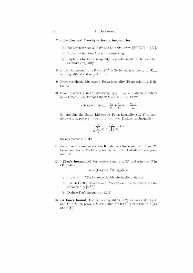
7. (The Fan and Cauchy–Schwarz inequalities)
(a) For any matrices X in Sn and U in On, prove ‖UT XU‖ = ‖X‖.(b) Prove the function λ is norm-preserving.
(c) Explain why Fan’s inequality is a refinement of the Cauchy–Schwarz inequality.
8. Prove the inequality tr Z + tr Z−1 ≥ 2n for all matrices Z in Sn++,
with equality if and only if Z = I.
9. Prove the Hardy–Littlewood–Polya inequality (Proposition 1.2.4) di-rectly.
10. Given a vector x in Rn+ satisfying x1x2 . . . xn = 1, define numbers
yk = 1/x1x2 . . . xk for each index k = 1, 2, . . . , n. Prove
x1 + x2 + . . . + xn =yn
y1+
y1
y2+ . . .
yn−1
yn.
By applying the Hardy–Littlewood–Polya inequality (1.2.4) to suit-able vectors, prove x1 + x2 + . . . + xn ≥ n. Deduce the inequality
1n
n∑1
zi ≥( n∏
1
zi
)1/n
for any vector z in Rn+.
11. For a fixed column vector s in Rn, define a linear map A : Sn → Rn
by setting AX = Xs for any matrix X in Sn. Calculate the adjointmap A∗.
12. ∗ (Fan’s inequality) For vectors x and y in Rn and a matrix U inOn, define
α = 〈Diag x,UT (Diag y)U〉.
(a) Prove α = xT Zy for some doubly stochastic matrix Z.
(b) Use Birkhoff’s theorem and Proposition 1.2.4 to deduce the in-equality α ≤ [x]T [y].
(c) Deduce Fan’s inequality (1.2.2).
13. (A lower bound) Use Fan’s inequality (1.2.2) for two matrices Xand Y in Sn to prove a lower bound for tr (XY ) in terms of λ(X)and λ(Y ).

1.2 Symmetric Matrices 13
14. ∗ (Level sets of perturbed log barriers)
(a) For δ in R++, prove the function
t ∈ R++ 7→ δt− log t
has compact level sets.(b) For c in Rn
++, prove the function
x ∈ Rn++ 7→ cT x−
n∑
i=1
log xi
has compact level sets.(c) For C in Sn
++, prove the function
X ∈ Sn++ 7→ 〈C, X〉 − log det X
has compact level sets. (Hint: Use Exercise 13.)
15. ∗ (Theobald’s condition) Assuming Fan’s inequality (1.2.2), com-plete the proof of Fan’s theorem (1.2.1) as follows. Suppose equalityholds in Fan’s inequality (1.2.2), and choose a spectral decomposition
X + Y = UT (Diag λ(X + Y ))U
for some matrix U in On.
(a) Prove λ(X)T λ(X + Y ) = 〈UT (Diagλ(X))U,X + Y 〉.(b) Apply Fan’s inequality (1.2.2) to the two inner products
〈X, X + Y 〉 and 〈UT (Diag λ(X))U, Y 〉to deduce X = UT (Diag λ(X))U .
(c) Deduce Fan’s theorem.
16. ∗∗ (Generalizing Theobald’s condition [122]) Consider a set ofmatrices X1, X2, . . . , Xm in Sn satisfying the conditions
tr (XiXj) = λ(Xi)T λ(Xj) for all i and j.
Generalize the argument of Exercise 15 to prove the entire set ofmatrices X1, X2, . . . , Xm has a simultaneous ordered spectral de-composition.
17. ∗∗ (Singular values and von Neumann’s lemma) Let Mn denotethe vector space of n×n real matrices. For a matrix A in Mn we definethe singular values of A by σi(A) =
√λi(AT A) for i = 1, 2, . . . , n,
and hence define a map σ : Mn → Rn. (Notice zero may be a singularvalue.)
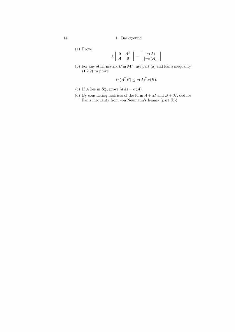
14 1. Background
(a) Prove
λ
[0 AT
A 0
]=
[σ(A)
[−σ(A)]
]
(b) For any other matrix B in Mn, use part (a) and Fan’s inequality(1.2.2) to prove
tr (AT B) ≤ σ(A)T σ(B).
(c) If A lies in Sn+, prove λ(A) = σ(A).
(d) By considering matrices of the form A+αI and B +βI, deduceFan’s inequality from von Neumann’s lemma (part (b)).
Chapter 2
Inequality Constraints
2.1 Optimality Conditions
Early in multivariate calculus we learn the significance of differentiabilityin finding minimizers. In this section we begin our study of the interplaybetween convexity and differentiability in optimality conditions.
For an initial example, consider the problem of minimizing a functionf : C → R on a set C in E. We say a point x in C is a local minimizerof f on C if f(x) ≥ f(x) for all points x in C close to x. The directionalderivative of a function f at x in a direction d ∈ E is
f ′(x; d) = limt↓0
f(x + td)− f(x)t
,
when this limit exists. When the directional derivative f ′(x; d) is actuallylinear in d (that is, f ′(x; d) = 〈a, d〉 for some element a of E) then we sayf is (Gateaux) differentiable at x, with (Gateaux) derivative ∇f(x) = a. Iff is differentiable at every point in C then we simply say f is differentiable(on C). An example we use quite extensively is the function X ∈ Sn
++ 7→log det X. An exercise shows this function is differentiable on Sn
++ withderivative X−1.
A convex cone which arises frequently in optimization is the normalcone to a convex set C at a point x ∈ C, written NC(x). This is the convexcone of normal vectors, vectors d in E such that 〈d, x− x〉 ≤ 0 for all pointsx in C.
Proposition 2.1.1 (First order necessary condition) Suppose that Cis a convex set in E and that the point x is a local minimizer of the functionf : C → R. Then for any point x in C, the directional derivative, if itexists, satisfies f ′(x; x − x) ≥ 0. In particular, if f is differentiable at x,then the condition −∇f(x) ∈ NC(x) holds.
15
16 2. Inequality Constraints
Proof. If some point x in C satisfies f ′(x;x − x) < 0, then all smallreal t > 0 satisfy f(x + t(x − x)) < f(x), but this contradicts the localminimality of x. 2
The case of this result where C is an open set is the canonical intro-duction to the use of calculus in optimization: local minimizers x must becritical points (that is, ∇f(x) = 0). This book is largely devoted to thestudy of first order necessary optimality conditions for a local minimizer ofa function subject to constraints. In that case local minimizers x may notlie in the interior of the set C of interest, so the normal cone NC(x) is notsimply 0.
The next result shows that when f is convex the first order conditionabove is sufficient for x to be a global minimizer of f on C.
Proposition 2.1.2 (First order sufficient condition) Suppose that theset C ⊂ E is convex and that the function f : C → R is convex. Thenfor any points x and x in C, the directional derivative f ′(x; x − x) existsin [−∞,+∞). If the condition f ′(x; x − x) ≥ 0 holds for all x in C, orin particular if the condition −∇f(x) ∈ NC(x) holds, then x is a globalminimizer of f on C.
Proof. A straightforward exercise using the convexity of f shows thefunction
t ∈ (0, 1] 7→ f(x + t(x− x))− f(x)t
is nondecreasing. The result then follows easily (Exercise 7). 2
In particular, any critical point of a convex function is a global minimizer.The following useful result illustrates what the first order conditions
become for a more concrete optimization problem. The proof is outlinedin Exercise 4.
Corollary 2.1.3 (First order conditions for linear constraints) Fora convex set C ⊂ E, a function f : C → R, a linear map A : E → Y (whereY is a Euclidean space) and a point b in Y, consider the optimizationproblem
inff(x) | x ∈ C, Ax = b. (2.1.4)
Suppose the point x ∈ intC satisfies Ax = b.
(a) If x is a local minimizer for the problem (2.1.4) and f is differentiableat x then ∇f(x) ∈ A∗Y.
(b) Conversely, if ∇f(x) ∈ A∗Y and f is convex then x is a global min-imizer for (2.1.4).
2.1 Optimality Conditions 17
The element y ∈ Y satisfying ∇f(x) = A∗y in the above result is calleda Lagrange multiplier. This kind of construction recurs in many differentforms in our development.
In the absence of convexity, we need second order information to tell usmore about minimizers. The following elementary result from multivariatecalculus is typical.
Theorem 2.1.5 (Second order conditions) Suppose the twice contin-uously differentiable function f : Rn → R has a critical point x. If x isa local minimizer then the Hessian ∇2f(x) is positive semidefinite. Con-versely, if the Hessian is positive definite then x is a local minimizer.
(In fact for x to be a local minimizer it is sufficient for the Hessian tobe positive semidefinite locally; the function x ∈ R 7→ x4 highlights thedistinction.)
To illustrate the effect of constraints on second order conditions, con-sider the framework of Corollary 2.1.3 (First order conditions for linearconstraints) in the case E = Rn, and suppose ∇f(x) ∈ A∗Y and f istwice continuously differentiable near x. If x is a local minimizer thenyT∇2f(x)y ≥ 0 for all vectors y in N(A). Conversely, if yT∇2f(x)y > 0for all nonzero y in N(A) then x is a local minimizer.
We are already beginning to see the broad interplay between analytic,geometric and topological ideas in optimization theory. A good illustrationis the separation result of Section 1.1, which we now prove.
Theorem 2.1.6 (Basic separation) Suppose that the set C ⊂ E is closedand convex, and that the point y does not lie in C. Then there exist a realb and a nonzero element a of E such that 〈a, y〉 > b ≥ 〈a, x〉 for all pointsx in C.
Proof. We may assume C is nonempty, and define a function f : E → R byf(x) = ‖x−y‖2/2. Now by the Weierstrass proposition (1.1.3) there existsa minimizer x for f on C, which by the First order necessary condition(2.1.1) satisfies −∇f(x) = y − x ∈ NC(x). Thus 〈y − x, x − x〉 ≤ 0 holdsfor all points x in C. Now setting a = y − x and b = 〈y − x, x〉 gives theresult. 2
We end this section with a rather less standard result, illustrating an-other idea which is important later, the use of “variational principles” totreat problems where minimizers may not exist, but which nonetheless have“approximate” critical points. This result is a precursor of a principle dueto Ekeland, which we develop in Section 7.1.
Proposition 2.1.7 If the function f : E → R is differentiable and boundedbelow then there are points where f has small derivative.
18 2. Inequality Constraints
Proof. Fix any real ε > 0. The function f + ε‖ · ‖ has bounded level sets,so has a global minimizer xε by the Weierstrass proposition (1.1.3). If thevector d = ∇f(xε) satisfies ‖d‖ > ε then, from the inequality
limt↓0
f(xε − td)− f(xε)t
= −〈∇f(xε), d〉 = −‖d‖2 < −ε‖d‖,
we would have for small t > 0 the contradiction
−tε‖d‖ > f(xε − td)− f(xε)= (f(xε − td) + ε‖xε − td‖)
− (f(xε) + ε‖xε‖) + ε(‖xε‖ − ‖xε − td‖)≥ −εt‖d‖
by definition of xε and the triangle inequality. Hence ‖∇f(xε)‖ ≤ ε. 2
Notice that the proof relies on consideration of a nondifferentiable func-tion, even though the result concerns derivatives.
Exercises and Commentary
The optimality conditions in this section are very standard (see for example[132]). The simple variational principle (Proposition 2.1.7) was suggestedby [95].
1. Prove the normal cone is a closed convex cone.
2. (Examples of normal cones) For the following sets C ⊂ E, checkC is convex and compute the normal cone NC(x) for points x in C:
(a) C a closed interval in R.
(b) C = B, the unit ball.
(c) C a subspace.
(d) C a closed halfspace: x | 〈a, x〉 ≤ b where 0 6= a ∈ E andb ∈ R.
(e) C = x ∈ Rn | xj ≥ 0 for all j ∈ J (for J ⊂ 1, 2, . . . , n).3. (Self-dual cones) Prove each of the following cones K satisfy the
relationship NK(0) = −K.
(a) Rn+
(b) Sn+
(c) x ∈ Rn | x1 ≥ 0, x21 ≥ x2
2 + x23 + · · ·+ x2
n

2.1 Optimality Conditions 19
4. (Normals to affine sets) Given a linear map A : E → Y (whereY is a Euclidean space) and a point b in Y, prove the normal coneto the set x ∈ E | Ax = b at any point in it is A∗Y . Hence deduceCorollary 2.1.3 (First order conditions for linear constraints).
5. Prove that the differentiable function x21 + x2
2(1− x1)3 has a uniquecritical point in R2, which is a local minimizer, but has no globalminimizer. Can this happen on R?
6. (The Rayleigh quotient)
(a) Let the function f : Rn \ 0 → R be continuous, satisfyingf(λx) = f(x) for all λ > 0 in R and nonzero x in Rn. Prove fhas a minimizer.
(b) Given a matrix A in Sn, define a function g(x) = xT Ax/‖x‖2for nonzero x in Rn. Prove g has a minimizer.
(c) Calculate ∇g(x) for nonzero x.
(d) Deduce that minimizers of g must be eigenvectors, and calculatethe minimum value.
(e) Find an alternative proof of part (d) by using a spectral decom-position of A.
(Another approach to this problem is given in Section 7.2, Exercise6.)
7. Suppose a convex function g : [0, 1] → R satisfies g(0) = 0. Prove thefunction t ∈ (0, 1] 7→ g(t)/t is nondecreasing. Hence prove that for aconvex function f : C → R and points x, x ∈ C ⊂ E, the quotient(f(x+ t(x− x))− f(x))/t is nondecreasing as a function of t in (0, 1],and complete the proof of Proposition 2.1.2.
8. ∗ (Nearest points)
(a) Prove that if a function f : C → R is strictly convex then it hasat most one global minimizer on C.
(b) Prove the function f(x) = ‖x−y‖2/2 is strictly convex on E forany point y in E.
(c) Suppose C is a nonempty, closed convex subset of E.
(i) If y is any point in E, prove there is a unique nearest point(or best approximation) PC(y) to y in C, characterized by
〈y − PC(y), x− PC(y)〉 ≤ 0 for all x ∈ C.
(ii) For any point x in C, deduce that d ∈ NC(x) holds if andonly if x is the nearest point in C to x + d.

20 2. Inequality Constraints
(iii) Deduce, furthermore, that any points y and z in E satisfy
‖PC(y)− PC(z)‖ ≤ ‖y − z‖,
so in particular the projection PC : E → C is continuous.
(d) Given a nonzero element a of E, calculate the nearest point inthe subspace x ∈ E | 〈a, x〉 = 0 to the point y ∈ E.
(e) (Projection on Rn+ and Sn
+) Prove the nearest point in Rn+
to a vector y in Rn is y+, where y+i = maxyi, 0 for each i. For
a matrix U in On and a vector y in Rn, prove that the nearestpositive semidefinite matrix to UT Diag yU is UT Diag y+U .
9. ∗ (Coercivity) Suppose that the function f : E → R is differentiableand satisfies the growth condition lim‖x‖→∞ f(x)/‖x‖ = +∞. Provethat the gradient map ∇f has range E. (Hint: Minimize the functionf(·)− 〈a, ·〉 for elements a of E.)
10. (a) Prove the function f : Sn++ → R defined by f(X) = tr X−1 is
differentiable on Sn++. (Hint: Expand the expression (X+tY )−1
as a power series.)
(b) Define a function f : Sn++ → R by f(X) = log det X. Prove
∇f(I) = I. Deduce ∇f(X) = X−1 for any X in Sn++.
11. ∗∗ (Kirchhoff’s law [9, Chapter 1]) Consider a finite, undirected,connected graph with vertex set V and edge set E. Suppose thatα and β in V are distinct vertices and that each edge ij in E hasan associated “resistance” rij > 0 in R. We consider the effect ofapplying a unit “potential difference” between the vertices α and β.Let V0 = V \ α, β, and for “potentials” x in RV0 we define the“power” p : RV0 → R by
p(x) =∑
ij∈E
(xi − xj)2
2rij,
where we set xα = 0 and xβ = 1.
(a) Prove the power function p has compact level sets.
(b) Deduce the existence of a solution to the following equations(describing “conservation of current”):
∑
j : ij∈E
xi − xj
rij= 0 for i in V0
xα = 0xβ = 1.
2.1 Optimality Conditions 21
(c) Prove the power function p is strictly convex.(d) Use part (a) of Exercise 8 to show that the conservation of cur-
rent equations in part (b) have a unique solution.
12. ∗∗ (Matrix completion [86]) For a set ∆ ⊂ (i, j) | 1 ≤ i ≤ j ≤ n,suppose the subspace L ⊂ Sn of matrices with (i, j)th entry of zerofor all (i, j) in ∆ satisfies L ∩ Sn
++ 6= ∅. By considering the problem(for C ∈ Sn
++)
inf〈C, X〉 − log det X |X ∈ L ∩ Sn++,
use Section 1.2, Exercise 14 and Corollary 2.1.3 (First order con-ditions for linear constraints) to prove there exists a matrix X inL ∩ Sn
++ with C −X−1 having (i, j)th entry of zero for all (i, j) notin ∆.
13. ∗∗ (BFGS update, cf. [80]) Given a matrix C in Sn++ and vectors
s and y in Rn satisfying sT y > 0, consider the problem
inf〈C, X〉 − log det X |Xs = y, X ∈ Sn++.
(a) Prove that for the problem above, the point
X =(y − δs)(y − δs)T
sT (y − δs)+ δI
is feasible for small δ > 0.(b) Prove the problem has an optimal solution using Section 1.2,
Exercise 14.(c) Use Corollary 2.1.3 (First order conditions for linear constraints)
to find the solution. (The solution is called the BFGS update ofC−1 under the secant condition Xs = y.)
(See also [61, p. 205].)
14. ∗∗ Suppose intervals I1, I2, . . . , In ⊂ R are nonempty and closed andthe function f : I1 × I2 × . . .× In → R is differentiable and boundedbelow. Use the idea of the proof of Proposition 2.1.7 to prove thatfor any ε > 0 there exists a point xε ∈ I1 × I2 × . . .× In satisfying
(−∇f(xε))j ∈ NIj (xεj) + [−ε, ε] (j = 1, 2, . . . , n).
15. ∗ (Nearest polynomial with a given root) Consider the Euclid-ean space of complex polynomials of degree no more than n, withinner product
⟨ n∑
j=0
xjzj ,
n∑
j=0
yjzj⟩
=n∑
j=0
xjyj .

22 2. Inequality Constraints
Given a polynomial p in this space, calculate the nearest polynomialwith a given complex root α, and prove the distance to this polyno-mial is (
∑nj=0 |α|2j)(−1/2)|p(α)|.
2.2 Theorems of the Alternative 23
2.2 Theorems of the Alternative
One well-trodden route to the study of first order conditions uses a class ofresults called “theorems of the alternative”, and, in particular, the Farkaslemma (which we derive at the end of this section). Our first approach,however, relies on a different theorem of the alternative.
Theorem 2.2.1 (Gordan) For any elements a0, a1, . . . , am of E, exactlyone of the following systems has a solution:
m∑
i=0
λiai = 0,
m∑
i=0
λi = 1, 0 ≤ λ0, λ1, . . . , λm ∈ R (2.2.2)
〈ai, x〉 < 0 for i = 0, 1, . . . , m, x ∈ E. (2.2.3)
Geometrically, Gordan’s theorem says that the origin does not lie in theconvex hull of the set a0, a1, . . . , am if and only if there is an openhalfspace y | 〈y, x〉 < 0 containing a0, a1, . . . , am (and hence its con-vex hull). This is another illustration of the idea of separation (in this casewe separate the origin and the convex hull).
Theorems of the alternative like Gordan’s theorem may be proved ina variety of ways, including separation and algorithmic approaches. Weemploy a less standard technique using our earlier analytic ideas and lead-ing to a rather unified treatment. It relies on the relationship between theoptimization problem
inff(x) | x ∈ E, (2.2.4)
where the function f is defined by
f(x) = log( m∑
i=0
exp〈ai, x〉), (2.2.5)
and the two systems (2.2.2) and (2.2.3). We return to the surprising func-tion (2.2.5) when we discuss conjugacy in Section 3.3.
Theorem 2.2.6 The following statements are equivalent:
(i) The function defined by (2.2.5) is bounded below.
(ii) System (2.2.2) is solvable.
(iii) System (2.2.3) is unsolvable.
Proof. The implications (ii) ⇒ (iii) ⇒ (i) are easy exercises, so it remainsto show (i) ⇒ (ii). To see this we apply Proposition 2.1.7. We deduce thatfor each k = 1, 2, . . . , there is a point xk in E satisfying
‖∇f(xk)‖ =∥∥∥
m∑
i=0
λki ai
∥∥∥ <1k
,
24 2. Inequality Constraints
where the scalars
λki =
exp〈ai, xk〉∑mr=0 exp〈ar, xk〉 > 0
satisfy∑m
i=0 λki = 1. Now the limit λ of any convergent subsequence of the
bounded sequence (λk) solves system (2.2.2). 2
The equivalence of (ii) and (iii) gives Gordan’s theorem.We now proceed by using Gordan’s theorem to derive the Farkas lemma,
one of the cornerstones of many approaches to optimality conditions. Theproof uses the idea of the projection onto a linear subspace Y of E. Noticefirst that Y becomes a Euclidean space by equipping it with the same innerproduct. The projection of a point x in E onto Y, written PYx, is simplythe nearest point to x in Y. This is well-defined (see Exercise 8 in Section2.1), and is characterized by the fact that x− PYx is orthogonal to Y. Astandard exercise shows PY is a linear map.
Lemma 2.2.7 (Farkas) For any points a1, a2, . . . , am and c in E, exactlyone of the following systems has a solution:
m∑
i=1
µiai = c, 0 ≤ µ1, µ2, . . . , µm ∈ R (2.2.8)
〈ai, x〉 ≤ 0 for i = 1, 2, . . . , m, 〈c, x〉 > 0, x ∈ E. (2.2.9)
Proof. Again, it is immediate that if system (2.2.8) has a solution thensystem (2.2.9) has no solution. Conversely, we assume (2.2.9) has no so-lution and deduce that (2.2.8) has a solution by using induction on thenumber of elements m. The result is clear for m = 0.
Suppose then that the result holds in any Euclidean space and for anyset of m − 1 elements and any element c. Define a0 = −c. ApplyingGordan’s theorem (2.2.1) to the unsolvability of (2.2.9) shows there arescalars λ0, λ1, . . . , λm ≥ 0 in R, not all zero, satisfying λ0c =
∑m1 λia
i.If λ0 > 0 the proof is complete, so suppose λ0 = 0 and without loss ofgenerality λm > 0.
Define a subspace of E by Y = y | 〈am, y〉 = 0, so by assumption thesystem
〈ai, y〉 ≤ 0 for i = 1, 2, . . . ,m− 1, 〈c, y〉 > 0, y ∈ Y,
or equivalently
〈PYai, y〉 ≤ 0 for i = 1, 2, . . . ,m− 1, 〈PYc, y〉 > 0, y ∈ Y,
has no solution.By the induction hypothesis applied to the subspace Y, there are non-
negative reals µ1, µ2, . . . , µm−1 satisfying∑m−1
i=1 µiPYai = PYc, so the
2.2 Theorems of the Alternative 25
vector c − ∑m−11 µia
i is orthogonal to the subspace Y = (span (am))⊥.Thus some real µm satisfies
µmam = c−m−1∑
1
µiai. (2.2.10)
If µm is nonnegative we immediately obtain a solution of (2.2.8), and ifnot then we can substitute am = −λ−1
m
∑m−11 λia
i in equation (2.2.10) toobtain a solution. 2
Just like Gordan’s theorem, the Farkas lemma has an important geomet-ric interpretation which gives an alternative approach to its proof (Exercise6): any point c not lying in the finitely generated cone
C = m∑
1
µiai∣∣∣ 0 ≤ µ1, µ2, . . . , µm ∈ R
(2.2.11)
can be separated from C by a hyperplane. If x solves system (2.2.9) then Cis contained in the closed halfspace a | 〈a, x〉 ≤ 0, whereas c is containedin the complementary open halfspace. In particular, it follows that anyfinitely generated cone is closed.
Exercises and Commentary
Gordan’s theorem appeared in [84], and the Farkas lemma appeared in [75].The standard modern approach to theorems of the alternative (Exercises7 and 8, for example) is via linear programming duality (see, for example,[53]). The approach we take to Gordan’s theorem was suggested by Hiriart–Urruty [95]. Schur-convexity (Exercise 9) is discussed extensively in [134].
1. Prove the implications (ii) ⇒ (iii) ⇒ (i) in Theorem 2.2.6.
2. (a) Prove the orthogonal projection PY : E → Y is a linear map.
(b) Give a direct proof of the Farkas lemma for the case m = 1.
3. Use the Basic separation theorem (2.1.6) to give another proof ofGordan’s theorem.
4. ∗ Deduce Gordan’s theorem from the Farkas lemma. (Hint: Considerthe elements (ai, 1) of the space E×R.)
5. ∗ (Caratheodory’s theorem [52]) Suppose ai | i ∈ I is a finiteset of points in E. For any subset J of I, define the cone
CJ = ∑
i∈J
µiai∣∣∣ 0 ≤ µi ∈ R, (i ∈ J)
.
26 2. Inequality Constraints
(a) Prove the cone CI is the union of those cones CJ for whichthe set ai | i ∈ J is linearly independent. Furthermore, provedirectly that any such cone CJ is closed.
(b) Deduce that any finitely generated cone is closed.(c) If the point x lies in conv ai | i ∈ I, prove that in fact there
is a subset J ⊂ I of size at most 1 + dimE such that x lies inconv ai | i ∈ J. (Hint: Apply part (a) to the vectors (ai, 1) inE×R.)
(d) Use part (c) to prove that if a subset of E is compact then so isits convex hull.
6. ∗ Give another proof of the Farkas lemma by applying the Basicseparation theorem (2.1.6) to the set defined by (2.2.11) and usingthe fact that any finitely generated cone is closed.
7. ∗∗ (Ville’s theorem) With the function f defined by (2.2.5) (withE = Rn), consider the optimization problem
inff(x) | x ≥ 0 (2.2.12)
and its relationship with the two systemsm∑
i=0
λiai ≥ 0,
m∑
i=0
λi = 1,
0 ≤ λ0, λ1, . . . , λm ∈ R (2.2.13)
and〈ai, x〉 < 0 for i = 0, 1, . . . , m, x ∈ Rn
+. (2.2.14)
Imitate the proof of Gordan’s theorem (using Section 2.1, Exercise14) to prove the following are equivalent:
(i) Problem (2.2.12) is bounded below.(ii) System (2.2.13) is solvable.(iii) System (2.2.14) is unsolvable.
Generalize by considering the problem inff(x) | xj ≥ 0 (j ∈ J).8. ∗∗ (Stiemke’s theorem) Consider the optimization problem (2.2.4)
and its relationship with the two systemsm∑
i=0
λiai = 0, 0 < λ0, λ1, . . . , λm ∈ R (2.2.15)
and
〈ai, x〉 ≤ 0 for i = 0, 1, . . . , m, not all 0, x ∈ E. (2.2.16)
Prove the following are equivalent:
2.2 Theorems of the Alternative 27
(i) Problem (2.2.4) has an optimal solution.(ii) System (2.2.15) is solvable.(iii) System (2.2.16) is unsolvable.
Hint: Complete the following steps.
(a) Prove (i) implies (ii) by Proposition 2.1.1.(b) Prove (ii) implies (iii).(c) If problem (2.2.4) has no optimal solution, prove that neither
does the problem
inf m∑
i=0
exp yi
∣∣∣ y ∈ K
, (2.2.17)
where K is the subspace (〈ai, x〉)mi=0 | x ∈ E ⊂ Rm+1. Hence,
by considering a minimizing sequence for (2.2.17), deduce system(2.2.16) is solvable.
Generalize by considering the problem inff(x) | xj ≥ 0 (j ∈ J).9. ∗∗ (Schur-convexity) The dual cone of the cone Rn
≥ is defined by(Rn≥
)+ = y ∈ Rn | 〈x, y〉 ≥ 0 for all x in Rn≥.
(a) Prove a vector y lies in (Rn≥)+ if and only if
j∑1
yi ≥ 0 for j = 1, 2, . . . , n− 1,n∑1
yi = 0.
(b) By writing∑j
1[x]i = maxk〈ak, x〉 for some suitable set of vectorsak, prove that the function x 7→ ∑j
1[x]i is convex. (Hint: UseSection 1.1, Exercise 7.)
(c) Deduce that the function x 7→ [x] is (Rn≥)+-convex, that is:
λ[x] + (1− λ)[y]− [λx + (1− λ)y] ∈ (Rn≥
)+ for 0 ≤ λ ≤ 1.
(d) Use Gordan’s theorem and Proposition 1.2.4 to deduce thatfor any x and y in Rn
≥, if y − x lies in (Rn≥)+ then x lies in
conv (Pny).(e) A function f : Rn
≥ → R is Schur-convex if
x, y ∈ Rn≥, y − x ∈ (
Rn≥
)+ ⇒ f(x) ≤ f(y).
Prove that if f is convex, then it is Schur-convex if and onlyif it is the restriction to Rn
≥ of a symmetric convex functiong : Rn → R (where by symmetric we mean g(x) = g(Πx) forany x in Rn and any permutation matrix Π).
28 2. Inequality Constraints
2.3 Max-functions
This section is an elementary exposition of the first order necessary con-ditions for a local minimizer of a differentiable function subject to differ-entiable inequality constraints. Throughout this section we use the term“differentiable” in the Gateaux sense, defined in Section 2.1. Our approach,which relies on considering the local minimizers of a max-function
g(x) = maxi=0,1,...,m
gi(x), (2.3.1)
illustrates a pervasive analytic idea in optimization: nonsmoothness. Evenif the functions g0, g1, . . . , gm are smooth, g may not be, and hence thegradient may no longer be a useful notion.
Proposition 2.3.2 (Directional derivatives of max-functions) Let xbe a point in the interior of a set C ⊂ E. Suppose that continuous functionsg0, g1, . . . , gm : C → R are differentiable at x, that g is the max-function(2.3.1), and define the index set K = i | gi(x) = g(x). Then for alldirections d in E, the directional derivative of g is given by
g′(x; d) = maxi∈K
〈∇gi(x), d〉. (2.3.3)
Proof. By continuity we can assume, without loss of generality, K =0, 1, . . . , m; those gi not attaining the maximum in (2.3.1) will not affectg′(x; d). Now for each i, we have the inequality
lim inft↓0
g(x + td)− g(x)t
≥ limt↓0
gi(x + td)− gi(x)t
= 〈∇gi(x), d〉.
Suppose
lim supt↓0
g(x + td)− g(x)t
> maxi〈∇gi(x), d〉.
Then some real sequence tk ↓ 0 and real ε > 0 satisfy
g(x + tkd)− g(x)tk
≥ maxi〈∇gi(x), d〉+ ε for all k ∈ N
(where N denotes the sequence of natural numbers). We can now choose asubsequence R of N and a fixed index j so that all integers k in R satisfyg(x + tkd) = gj(x + tkd). In the limit we obtain the contradiction
〈∇gj(x), d〉 ≥ maxi〈∇gi(x), d〉+ ε.
Hence
lim supt↓0
g(x + td)− g(x)t
≤ maxi〈∇gi(x), d〉,

2.3 Max-functions 29
and the result follows. 2
For most of this book we consider optimization problems of the form
inf f(x)subject to gi(x) ≤ 0 for i ∈ I
hj(x) = 0 for j ∈ Jx ∈ C,
(2.3.4)
where C is a subset of E, I and J are finite index sets, and the objectivefunction f and inequality and equality constraint functions gi (i ∈ I) andhj (j ∈ J), respectively, are continuous from C to R. A point x in C isfeasible if it satisfies the constraints, and the set of all feasible x is called thefeasible region. If the problem has no feasible points, we call it inconsistent.We say a feasible point x is a local minimizer if f(x) ≥ f(x) for all feasiblex close to x. We aim to derive first order necessary conditions for localminimizers.
We begin in this section with the differentiable inequality constrainedproblem
inf f(x)subject to gi(x) ≤ 0 for i = 1, 2, . . . , m
x ∈ C.
(2.3.5)
For a feasible point x we define the active set I(x) = i | gi(x) = 0. Forthis problem, assuming x ∈ intC, we call a vector λ ∈ Rm
+ a Lagrangemultiplier vector for x if x is a critical point of the Lagrangian
L(x;λ) = f(x) +m∑
i=1
λigi(x)
(in other words, ∇f(x) +∑
λi∇gi(x) = 0), and complementary slacknessholds: λi = 0 for indices i not in I(x).
Theorem 2.3.6 (Fritz John conditions) Suppose problem (2.3.5) has alocal minimizer x ∈ intC. If the functions f, gi (i ∈ I(x)) are differentiableat x then there exist λ0, λi ∈ R+ (i ∈ I(x)), not all zero, satisfying
λ0∇f(x) +∑
i∈I(x)
λi∇gi(x) = 0.
Proof. Consider the function
g(x) = maxf(x)− f(x), gi(x) | i ∈ I(x).Since x is a local minimizer for the problem (2.3.5), it is a local minimizerof the function g, so all directions d ∈ E satisfy the inequality
g′(x; d) = max〈∇f(x), d〉, 〈∇gi(x), d〉 | i ∈ I(x) ≥ 0,

30 2. Inequality Constraints
by the First order necessary condition (2.1.1) and Proposition 2.3.2 (Direc-tional derivatives of max-functions). Thus the system
〈∇f(x), d〉 < 0, 〈∇gi(x), d〉 < 0 for i ∈ I(x)
has no solution, and the result follows by Gordan’s theorem (2.2.1). 2
One obvious disadvantage remains with the Fritz John first order condi-tions above: if λ0 = 0 then the conditions are independent of the objectivefunction f . To rule out this possibility we need to impose a regularity con-dition or “constraint qualification”, an approach which is another recurringtheme. The easiest such condition in this context is simply the linear in-dependence of the gradients of the active constraints ∇gi(x) | i ∈ I(x).The culminating result of this section uses the following weaker condition.
Assumption 2.3.7 (The Mangasarian–Fromovitz constraint qual-ification) There is a direction d in E satisfying 〈∇gi(x), d〉 < 0 for allindices i in the active set I(x).
Theorem 2.3.8 (Karush–Kuhn–Tucker conditions) Suppose problem(2.3.5) has a local minimizer x in intC. If the functions f, gi (for i ∈I(x)) are differentiable at x, and if the Mangasarian–Fromovitz constraintqualification (2.3.7) holds, then there is a Lagrange multiplier vector for x.
Proof. By the trivial implication in Gordan’s theorem (2.2.1), the con-straint qualification ensures λ0 6= 0 in the Fritz John conditions (2.3.6).
2
Exercises and Commentary
The approach to first order conditions of this section is due to [95]. TheFritz John conditions appeared in [107]. The Karush–Kuhn–Tucker condi-tions were first published (under a different regularity condition) in [117],although the conditions appear earlier in an unpublished master’s thesis[111]. The Mangasarian–Fromovitz constraint qualification appeared in[133]. A nice collection of optimization problems involving the determi-nant, similar to Exercise 8 (Minimum volume ellipsoid), appears in [47](see also [183]). The classic reference for inequalities is [91].
1. Prove by induction that if the functions g0, g1, . . . , gm : E → R areall continuous at the point x then so is the max-function g(x) =maxigi(x).
2. (Failure of Karush–Kuhn–Tucker) Consider the following prob-lem:
inf (x1 + 1)2 + x22
subject to −x31 + x2
2 ≤ 0x ∈ R2.
2.3 Max-functions 31
(a) Sketch the feasible region and hence solve the problem.
(b) Find multipliers λ0 and λ satisfying the Fritz John conditions(2.3.6).
(c) Prove there exists no Lagrange multiplier vector for the optimalsolution. Explain why not.
3. (Linear independence implies Mangasarian–Fromovitz) If theset of vectors a1, a2, . . . , am in E is linearly independent, provedirectly there exists a direction d in E satisfying 〈ai, d〉 < 0 for i =1, 2, . . . ,m.
4. For each of the following problems, explain why there must existan optimal solution, and find it by using the Karush–Kuhn–Tuckerconditions.
(a) inf x21 + x2
2
subject to −2x1 − x2 + 10 ≤ 0−x1 ≤ 0.
(b) inf 5x21 + 6x2
2
subject to x1 − 4 ≤ 025− x2
1 − x22 ≤ 0.
5. (Cauchy–Schwarz and steepest descent) For a nonzero vector yin E, use the Karush–Kuhn–Tucker conditions to solve the problem
inf〈y, x〉 | ‖x‖2 ≤ 1.
Deduce the Cauchy–Schwarz inequality.
6. ∗ (Holder’s inequality) For real p > 1, define q by p−1 + q−1 = 1,and for x in Rn define
‖x‖p =( n∑
1
|xi|p)1/p
.
For a nonzero vector y in Rn, consider the optimization problem
inf〈y, x〉 | ‖x‖pp ≤ 1. (2.3.9)
(a) Prove ddu |u|p/p = u|u|p−2 for all real u.
(b) Prove reals u and v satisfy v = u|u|p−2 if and only if u = v|v|q−2.
(c) Prove problem (2.3.9) has a nonzero optimal solution.
(d) Use the Karush–Kuhn–Tucker conditions to find the unique op-timal solution.

32 2. Inequality Constraints
(e) Deduce that any vectors x and y in Rn satisfy 〈y, x〉 ≤ ‖y‖q‖x‖p.
(We develop another approach to this theory in Section 4.1, Exercise11.)
7. ∗ Consider a matrix A in Sn++ and a real b > 0.
(a) Assuming the problem
inf− log det X | trAX ≤ b, X ∈ Sn++
has a solution, find it.
(b) Repeat using the objective function tr X−1.
(c) Prove the problems in parts (a) and (b) have optimal solutions.(Hint: Section 1.2, Exercise 14.)
8. ∗∗ (Minimum volume ellipsoid)
(a) For a point y in Rn and the function g : Sn → R defined byg(X) = ‖Xy‖2, prove ∇g(X) = XyyT + yyT X for all matricesX in Sn.
(b) Consider a set y1, y2, . . . , ym ⊂ Rn. Prove this set spans Rn
if and only if the matrix∑
i yi(yi)T is positive definite.
Now suppose the vectors y1, y2, . . . , ym span Rn.
(c) Prove the problem
inf − log det Xsubject to ‖Xyi‖2 − 1 ≤ 0 for i = 1, 2, . . . , m
X ∈ Sn++
has an optimal solution. (Hint: Use part (b) and Section 1.2,Exercise 14.)
Now suppose X is an optimal solution for the problem in part (c). (Inthis case the set y ∈ Rn | ‖Xy‖ ≤ 1 is a minimum volume ellipsoid(centered at the origin) containing the vectors y1, y2, . . . , ym.)
(d) Show the Mangasarian–Fromovitz constraint qualification holdsat X by considering the direction d = −X.
(e) Write down the Karush–Kuhn–Tucker conditions that X mustsatisfy.
(f) When y1, y2, . . . , ym is the standard basis of Rn, the optimalsolution of the problem in part (c) is X = I. Find the corre-sponding Lagrange multiplier vector.

Chapter 3
Fenchel Duality
3.1 Subgradients and Convex Functions
We have already seen, in the First order sufficient condition (2.1.2), onebenefit of convexity in optimization: critical points of convex functions areglobal minimizers. In this section we extend the types of functions weconsider in two important ways:
(i) We do not require f to be differentiable.
(ii) We allow f to take the value +∞.
Our derivation of first order conditions in Section 2.3 illustrates theutility of considering nonsmooth functions even in the context of smoothproblems. Allowing the value +∞ lets us rephrase a problem like
infg(x) | x ∈ Cas inf(g + δC), where the indicator function δC(x) is 0 for x in C and +∞otherwise.
The domain of a function f : E → (∞,+∞] is the set
dom f = x ∈ E | f(x) < +∞.We say f is convex if it is convex on its domain, and proper if its domainis nonempty. We call a function g : E → [−∞,+∞) concave if −g isconvex, although for reasons of simplicity we will consider primarily convexfunctions. If a convex function f satisfies the stronger condition
f(λx + µy) ≤ λf(x) + µf(y) for all x, y ∈ E, λ, µ ∈ R+
we say f is sublinear. If f(λx) = λf(x) for all x in E and λ in R+ thenf is positively homogeneous: in particular this implies f(0) = 0. (Recall
33

34 3. Fenchel Duality
the convention 0 · (+∞) = 0.) If f(x + y) ≤ f(x) + f(y) for all x and yin E then we say f is subadditive. It is immediate that if the function fis sublinear then −f(x) ≤ f(−x) for all x in E. The lineality space of asublinear function f is the set
lin f = x ∈ E | −f(x) = f(−x).
The following result (whose proof is left as an exercise) shows this set is asubspace.
Proposition 3.1.1 (Sublinearity) A function f : E → (∞, +∞] is sub-linear if and only if it is positively homogeneous and subadditive. For asublinear function f , the lineality space lin f is the largest subspace of E onwhich f is linear.
As in the First order sufficient condition (2.1.2), it is easy to checkthat if the point x lies in the domain of the convex function f then thedirectional derivative f ′(x; ·) is well-defined and positively homogeneous,taking values in [−∞, +∞]. The core of a set C (written core (C)) is theset of points x in C such that for any direction d in E, x + td lies in C forall small real t. This set clearly contains the interior of C, although it maybe larger (Exercise 2).
Proposition 3.1.2 (Sublinearity of the directional derivative) If thefunction f : E → (∞, +∞] is convex then, for any point x in core (dom f),the directional derivative f ′(x; ·) is everywhere finite and sublinear.
Proof. For d in E and nonzero t in R, define
g(d; t) =f(x + td)− f(x)
t.
By convexity we deduce, for 0 < t ≤ s ∈ R, the inequality
g(d;−s) ≤ g(d;−t) ≤ g(d; t) ≤ g(d; s).
Since x lies in core (dom f), for small s > 0 both g(d;−s) and g(d; s) arefinite, so as t ↓ 0 we have
+∞ > g(d; s) ≥ g(d; t) ↓ f ′(x; d) ≥ g(d;−s) > −∞. (3.1.3)
Again by convexity we have, for any directions d and e in E and real t > 0,
g(d + e; t) ≤ g(d; 2t) + g(e; 2t).
Now letting t ↓ 0 gives subadditivity of f ′(x; ·). The positive homogeneityis easy to check. 2

3.1 Subgradients and Convex Functions 35
The idea of the derivative is fundamental in analysis because it allowsus to approximate a wide class of functions using linear functions. In opti-mization we are concerned specifically with the minimization of functions,and hence often a one-sided approximation is sufficient. In place of the gra-dient we therefore consider subgradients, those elements φ of E satisfying
〈φ, x− x〉 ≤ f(x)− f(x) for all points x in E. (3.1.4)
We denote the set of subgradients (called the subdifferential) by ∂f(x),defining ∂f(x) = ∅ for x not in dom f . The subdifferential is always a closedconvex set. We can think of ∂f(x) as the value at x of the “multifunction”or “set-valued map” ∂f : E → E. The importance of such maps is anotherof our themes. We define its domain
dom ∂f = x ∈ E | ∂f(x) 6= ∅
(Exercise 19). We say f is essentially strictly convex if it is strictly convexon any convex subset of dom ∂f .
The following very easy observation suggests the fundamental signifi-cance of subgradients in optimization.
Proposition 3.1.5 (Subgradients at optimality) For any proper func-tion f : E → (∞,+∞], the point x is a (global) minimizer of f if and onlyif the condition 0 ∈ ∂f(x) holds.
Alternatively put, minimizers of f correspond exactly to “zeroes” of ∂f .The derivative is a local property whereas the subgradient definition
(3.1.4) describes a global property. The main result of this section showsthat the set of subgradients of a convex function is usually nonempty, andthat we can describe it locally in terms of the directional derivative. Webegin with another simple exercise.
Proposition 3.1.6 (Subgradients and directional derivatives) If thefunction f : E → (∞, +∞] is convex and the point x lies in dom f , thenan element φ of E is a subgradient of f at x if and only if it satisfies〈φ, ·〉 ≤ f ′(x; ·).
The idea behind the construction of a subgradient for a function f thatwe present here is rather simple. We recursively construct a decreasingsequence of sublinear functions which, after translation, minorize f . Ateach step we guarantee one extra direction of linearity. The basic step issummarized in the following exercise.
Lemma 3.1.7 Suppose that the function p : E → (∞,+∞] is sublinearand that the point x lies in core (dom p). Then the function q(·) = p′(x; ·)satisfies the conditions

36 3. Fenchel Duality
(i) q(λx) = λp(x) for all real λ,
(ii) q ≤ p, and
(iii) lin q ⊃ lin p + span x.With this tool we are now ready for the main result, which gives condi-
tions guaranteeing the existence of a subgradient. Proposition 3.1.6 showedhow to identify subgradients from directional derivatives; this next resultshows how to move in the reverse direction.
Theorem 3.1.8 (Max formula) If the function f : E → (∞,+∞] isconvex then any point x in core (dom f) and any direction d in E satisfy
f ′(x; d) = max〈φ, d〉 | φ ∈ ∂f(x). (3.1.9)
In particular, the subdifferential ∂f(x) is nonempty.
Proof. In view of Proposition 3.1.6, we simply have to show that for anyfixed d in E there is a subgradient φ satisfying 〈φ, d〉 = f ′(x; d). Choosea basis e1, e2, . . . , en for E with e1 = d if d is nonzero. Now definea sequence of functions p0, p1, . . . , pn recursively by p0(·) = f ′(x; ·), andpk(·) = p′k−1(ek; ·) for k = 1, 2, . . . , n. We essentially show that pn(·) is therequired subgradient.
First note that, by Proposition 3.1.2, each pk is everywhere finite andsublinear. By part (iii) of Lemma 3.1.7 we know
lin pk ⊃ lin pk−1 + span ek for k = 1, 2, . . . , n,
so pn is linear. Thus there is an element φ of E satisfying 〈φ, ·〉 = pn(·).Part (ii) of Lemma 3.1.7 implies pn ≤ pn−1 ≤ . . . ≤ p0, so certainly, by
Proposition 3.1.6, any point x in E satisfies
pn(x− x) ≤ p0(x− x) = f ′(x; x− x) ≤ f(x)− f(x).
Thus φ is a subgradient. If d is zero then we have pn(0) = 0 = f ′(x; 0).Finally, if d is nonzero then by part (i) of Lemma 3.1.7 we see
pn(d) ≤ p0(d) = p0(e1) = −p′0(e1;−e1) =−p1(−e1) = −p1(−d) ≤ −pn(−d) = pn(d),
whence pn(d) = p0(d) = f ′(x; d). 2
Corollary 3.1.10 (Differentiability of convex functions) Suppose thefunction f : E → (∞, +∞] is convex and the point x lies in core (dom f).Then f is Gateaux differentiable at x exactly when f has a unique subgra-dient at x (in which case this subgradient is the derivative).
3.1 Subgradients and Convex Functions 37
We say the convex function f is essentially smooth if it is Gateaux dif-ferentiable on dom ∂f . (In this definition, we also require f to be “lowersemicontinuous”; we defer discussion of lower semicontinuity until we needit, in Section 4.2.) We see later (Section 4.1, Exercise 21) that a functionis essentially smooth if and only if its subdifferential is always singleton orempty.
The Max formula (Theorem 3.1.8) shows that convex functions typicallyhave subgradients. In fact this property characterizes convexity (Exercise12). This leads to a number of important ways of recognizing convex func-tions, one of which is the following example. Notice how a locally definedanalytic condition results in a global geometric conclusion. The proof isoutlined in the exercises.
Theorem 3.1.11 (Hessian characterization of convexity) Given anopen convex set S ⊂ Rn, suppose the continuous function f : cl S → R istwice continuously differentiable on S. Then f is convex if and only if itsHessian matrix is positive semidefinite everywhere on S.
Exercises and Commentary
The algebraic proof of the Max formula we follow here is due to [22]. Theexercises below develop several standard characterizations of convexity—see for example [167]. The convexity of − log det (Exercise 21) may befound in [99], for example. We shall see that the core and interior of aconvex set in fact coincide (Theorem 4.1.4).
1. Prove Proposition 3.1.1 (Sublinearity).
2. (Core versus interior) Consider the set in R2
D = (x, y) | y = 0 or |y| ≥ x2.
Prove 0 ∈ core (D) \ int (D).
3. Prove the subdifferential is a closed convex set.
4. (Subgradients and normal cones) If a point x lies in a set C ⊂ E,prove ∂δC(x) = NC(x).
5. Prove the following functions x ∈ R 7→ f(x) are convex and calculate∂f :
(a) |x|(b) δR+
(c)−√x if x ≥ 0
+∞ otherwise
38 3. Fenchel Duality
(d)
0 if x < 01 if x = 0+∞ otherwise.
6. Prove Proposition 3.1.6 (Subgradients and directional derivatives).
7. Prove Lemma 3.1.7.
8. (Subgradients of norm) Calculate ∂‖ · ‖. Generalize your result toan arbitrary sublinear function.
9. (Subgradients of maximum eigenvalue) Prove
∂λ1(0) = Y ∈ Sn+ | trY = 1.
10. ∗∗ For any vector µ in the cone Rn≥, prove
∂〈µ, [·]〉(0) = conv (Pnµ)
(see Section 2.2, Exercise 9 (Schur-convexity)).
11. ∗ Define a function f : Rn → R by f(x1, x2, . . . , xn) = maxjxj,let x = 0 and d = (1, 1, . . . , 1)T , and let ek = (1, 1, . . . , 1, 0, . . . , 0)T
(ending in (k − 1) zeroes). Calculate the functions pk defined inthe proof of Theorem 3.1.8 (Max formula), using Proposition 2.3.2(Directional derivatives of max functions).
12. ∗ (Recognizing convex functions) Suppose the set S ⊂ Rn isopen and convex, and consider a function f : S → R. For pointsx 6∈ S, define f(x) = +∞.
(a) Prove ∂f(x) is nonempty for all x in S if and only if f is convex.(Hint: For points u and v in S and real λ in [0, 1], use thesubgradient inequality (3.1.4) at the points x = λu + (1 − λ)vand x = u, v to check the definition of convexity.)
(b) Prove that if I ⊂ R is an open interval and g : I → R isdifferentiable then g is convex if and only if g′ is nondecreasingon I, and g is strictly convex if and only if g′ is strictly increasingon I. Deduce that if g is twice differentiable then g is convex ifand only if g′′ is nonnegative on I, and g is strictly convex if g′′
is strictly positive on I.
(c) Deduce that if f is twice continuously differentiable on S then fis convex if and only if its Hessian matrix is positive semidefiniteeverywhere on S, and f is strictly convex if its Hessian matrix ispositive definite everywhere on S. (Hint: Apply part (b) to thefunction g defined by g(t) = f(x + td) for small real t, points xin S, and directions d in E.)
3.1 Subgradients and Convex Functions 39
(d) Find a strictly convex function f : (−1, 1) → R with f ′′(0) = 0.
(e) Prove that a continuous function h : cl S → R is convex if andonly if its restriction to S is convex. What about strictly convexfunctions?
13. (Local convexity) Suppose the function f : Rn → R is twice con-tinuously differentiable near 0 and ∇2f(0) is positive definite. Provef |δB is convex for some real δ > 0.
14. (Examples of convex functions) As we shall see in Section 4.2,most natural convex functions occur in pairs. The table in Section3.3 lists many examples on R. Use Exercise 12 to prove each functionf and f∗ in the table is convex.
15. (Examples of convex functions) Prove the following functions ofx ∈ R are convex:
(a) log( sinh ax
sinhx
)for a ≥ 1.
(b) log(eax − 1
ex − 1
)for a ≥ 1.
16. ∗ (Bregman distances [48]) For a function φ : E → (∞, +∞]that is strictly convex and differentiable on int (dom φ), define theBregman distance dφ : dom φ× int (dom φ) → R by
dφ(x, y) = φ(x)− φ(y)− φ′(y)(x− y).
(a) Prove dφ(x, y) ≥ 0, with equality if and only if x = y.
(b) Compute dφ when φ(t) = t2/2 and when φ is the function pdefined in Exercise 27.
(c) Suppose φ is three times differentiable. Prove dφ is convex ifand only if −1/φ′′ is convex on int (dom φ).
(d) Extend the results above to the function
Dφ : (domφ)n × (int (dom φ))n → R
defined by Dφ(x, y) =∑
i dφ(xi, yi).
17. ∗ (Convex functions on R2) Prove the following functions of x ∈R2 are convex:
(a)
(x1 − x2)(log x1 − log x2) if x ∈ R2++
0 if x = 0+∞ otherwise.
(Hint: See Exercise 16.)

40 3. Fenchel Duality
(b)
x21
x2if x2 > 0
0 if x = 0+∞ otherwise.
18. ∗ Prove the function
f(x) =−(x1x2 . . . xn)1/n if x ∈ Rn
+
+∞ otherwise
is convex.
19. (Domain of subdifferential) If the function f : R2 → (∞,+∞] isdefined by
f(x1, x2) =
max1−√x1, |x2| if x1 ≥ 0+∞ otherwise,
prove that f is convex but that dom ∂f is not convex.
20. ∗ (Monotonicity of gradients) Suppose that the set S ⊂ Rn isopen and convex and that the function f : S → R is differentiable.Prove f is convex if and only if
〈∇f(x)−∇f(y), x− y〉 ≥ 0 for all x, y ∈ S,
and f is strictly convex if and only if the above inequality holdsstrictly whenever x 6= y. (You may use Exercise 12.)
21. ∗∗ (The log barrier) Use Exercise 20 (Monotonicity of gradients),Exercise 10 in Section 2.1 and Exercise 8 in Section 1.2 to prove thatthe function f : Sn
++ → R defined by f(X) = − log det X is strictlyconvex. Deduce the uniqueness of the minimum volume ellipsoid inSection 2.3, Exercise 8, and the matrix completion in Section 2.1,Exercise 12.
22. Prove the function (2.2.5) is convex on Rn by calculating its Hessian.
23. ∗ If the function f : E → (∞, +∞] is essentially strictly convex, proveall distinct points x and y in E satisfy ∂f(x) ∩ ∂f(y) = ∅. Deducethat f has at most one minimizer.
24. (Minimizers of essentially smooth functions) Prove that anyminimizer of an essentially smooth function f must lie in core (dom f).
25. ∗∗ (Convex matrix functions) Consider a matrix C in Sn+.

3.1 Subgradients and Convex Functions 41
(a) For matrices X in Sn++ and D in Sn, use a power series expansion
to proved2
dt2tr (C(X + tD)−1)
∣∣∣t=0
≥ 0.
(b) Deduce X ∈ Sn++ 7→ tr (CX−1) is convex.
(c) Prove similarly the function X ∈ Sn 7→ tr (CX2) and the func-tion X ∈ Sn
+ 7→ −tr (CX1/2) are convex.
26. ∗∗ (Log-convexity) Given a convex set C ⊂ E, we say that a func-tion f : C → R++ is log-convex if log f(·) is convex.
(a) Prove any log-convex function is convex, using Section 1.1, Ex-ercise 9 (Composing convex functions).
(b) If a polynomial p : R → R has all real roots, prove 1/p is log-convex on any interval on which p is strictly positive.
(c) One version of Holder’s inequality states, for real p, q > 1 satis-fying p−1 + q−1 = 1 and functions u, v : R+ → R,
∫uv ≤
( ∫|u|p
)1/p( ∫|v|q
)1/q
when the right hand side is well-defined. Use this to prove thegamma function Γ : R → R given by
Γ(x) =∫ ∞
0
tx−1e−t dt
is log-convex.
27. ∗∗ (Maximum entropy [36]) Define a convex function p : R →(−∞, +∞] by
p(u) =
u log u− u if u > 00 if u = 0+∞ if u < 0
and a convex function f : Rn → (−∞, +∞] by
f(x) =n∑
i=1
p(xi).
Suppose x lies in the interior of Rn+.
(a) Prove f is strictly convex on Rn+ with compact level sets.
(b) Prove f ′(x; x − x) = −∞ for any point x on the boundary ofRn
+.
42 3. Fenchel Duality
(c) Suppose the map G : Rn → Rm is linear with Gx = b. Provefor any vector c in Rn that the problem
inff(x) + 〈c, x〉 |Gx = b, x ∈ Rn
has a unique optimal solution x, lying in Rn++.
(d) Use Corollary 2.1.3 (First order conditions for linear constraints)to prove that some vector λ in Rm satisfies ∇f(x) = G∗λ − c,and deduce xi = exp(G∗λ− c)i.
28. ∗∗ (DAD problems [36]) Consider the following example of Exercise27 (Maximum entropy). Suppose the k × k matrix A has each entryaij nonnegative. We say A has doubly stochastic pattern if there isa doubly stochastic matrix with exactly the same zero entries as A.Define a set Z = (i, j)|aij > 0, and let RZ denote the set of vectorswith components indexed by Z and RZ
+ denote those vectors in RZ
with all nonnegative components. Consider the problem
inf∑
(i,j)∈Z(p(xij)− xij log aij)subject to
∑i:(i,j)∈Z xij = 1 for j = 1, 2, . . . , k∑j:(i,j)∈Z xij = 1 for i = 1, 2, . . . , k
x ∈ RZ .
(a) Suppose A has doubly stochastic pattern. Prove there is a pointx in the interior of RZ
+ which is feasible for the problem above.Deduce that the problem has a unique optimal solution x, and,for some vectors λ and µ in Rk, x satisfies
xij = aij exp(λi + µj) for (i, j) ∈ Z.
(b) Deduce that A has doubly stochastic pattern if and only if thereare diagonal matrices D1 and D2 with strictly positive diagonalentries and D1AD2 doubly stochastic.
29. ∗∗ (Relativizing the Max formula) If f : E → (∞, +∞] is aconvex function then for points x in ri (dom f) and directions d in E,prove the subdifferential ∂f(x) is nonempty and
f ′(x; d) = sup〈φ, d〉 | φ ∈ ∂f(x),
with attainment when finite.
3.2 The Value Function 43
3.2 The Value Function
In this section we describe another approach to the Karush–Kuhn–Tuckerconditions (2.3.8) in the convex case using the existence of subgradients weestablished in the previous section. We consider an (inequality-constrained)convex program
inff(x) | gi(x) ≤ 0 for i = 1, 2, . . . , m, x ∈ E, (3.2.1)
where the functions f, g1, g2, . . . , gm : E → (∞, +∞] are convex and satisfy∅ 6= dom f ⊂ ∩idom gi. Denoting the vector with components gi(x) byg(x), the function L : E×Rm
+ → (∞, +∞] defined by
L(x;λ) = f(x) + λT g(x), (3.2.2)
is called the Lagrangian. A feasible solution is a point x in dom f satisfyingthe constraints.
We should emphasize that the term “Lagrange multiplier” has differentmeanings in different contexts. In the present context we say a vector λ ∈Rm
+ is a Lagrange multiplier vector for a feasible solution x if x minimizesthe function L( · ; λ) over E and λ satisfies the complementary slacknessconditions: λi = 0 whenever gi(x) < 0.
We can often use the following principle to solve simple optimizationproblems.
Proposition 3.2.3 (Lagrangian sufficient conditions) If the point xis feasible for the convex program (3.2.1) and there is a Lagrange multipliervector, then x is optimal.
The proof is immediate, and in fact does not rely on convexity.The Karush–Kuhn–Tucker conditions (2.3.8) are a converse to the above
result when the functions f, g1, g2, . . . , gm are convex and differentiable.We next follow a very different, and surprising, route to this result, cir-cumventing differentiability. We perturb the problem (3.2.1), and analyzethe resulting (optimal) value function v : Rm → [−∞,+∞], defined by theequation
v(b) = inff(x) | g(x) ≤ b. (3.2.4)
We show that Lagrange multiplier vectors λ correspond to subgradients ofv (Exercise 9).
Our old definition of convexity for functions does not naturally extendto functions h : E → [−∞, +∞] (due to the possible occurrence of ∞−∞).To generalize the definition we introduce the idea of the epigraph of h:
epi (h) = (y, r) ∈ E×R | h(y) ≤ r, (3.2.5)
44 3. Fenchel Duality
and we say h is a convex function if epi (h) is a convex set. An exerciseshows in this case that the domain
dom (h) = y | h(y) < +∞
is convex, and further that the value function v defined by equation (3.2.4)is convex. We say h is proper if dom h is nonempty and h never takes thevalue −∞: if we wish to demonstrate the existence of subgradients for vusing the results in the previous section then we need to exclude −∞.
Lemma 3.2.6 If the function h : E → [−∞, +∞] is convex and somepoint y in core (domh) satisfies h(y) > −∞, then h never takes the value−∞.
Proof. Suppose some point y in E satisfies h(y) = −∞. Since y lies incore (dom h), there is a real t > 0 with y + t(y − y) in dom (h), and hencea real r with (y + t(y − y), r) in epi (h). Now for any real s, (y, s) lies inepi (h), so we know
(y,
r + ts
1 + t
)=
11 + t
(y + t(y − y), r) +t
1 + t(y, s) ∈ epi (h),
Letting s → −∞ gives a contradiction. 2
In Section 2.3 we saw that the Karush–Kuhn–Tucker conditions neededa regularity condition. In this approach we will apply a different condition,known as the Slater constraint qualification, for the problem (3.2.1):
There exists x in dom (f) with gi(x) < 0 for i = 1, 2, . . . , m. (3.2.7)
Theorem 3.2.8 (Lagrangian necessary conditions) Suppose that thepoint x in dom (f) is optimal for the convex program (3.2.1) and that theSlater condition (3.2.7) holds. Then there is a Lagrange multiplier vectorfor x.
Proof. Defining the value function v by equation (3.2.4), certainly v(0) >−∞, and the Slater condition shows 0 ∈ core (dom v), so in particularLemma 3.2.6 shows that v never takes the value −∞. (An incidental con-sequence, from Section 4.1, is the continuity of v at 0.) We now deduce theexistence of a subgradient −λ of v at 0, by the Max formula (3.1.8).
Any vector b in Rm+ obviously satisfies g(x) ≤ b, whence the inequality
f(x) = v(0) ≤ v(b) + λT b ≤ f(x) + λT b.
Hence, λ lies in Rm+ . Furthermore, any point x in dom f clearly satisfies
f(x) ≥ v(g(x)) ≥ v(0)− λT g(x) = f(x)− λT g(x).
3.2 The Value Function 45
The case x = x, using the inequalities λ ≥ 0 and g(x) ≤ 0, shows λT g(x) =0, which yields the complementary slackness conditions. Finally, all pointsx in dom f must satisfy f(x) + λT g(x) ≥ f(x) = f(x) + λT g(x). 2
In particular, if in the above result x lies in core (dom f) and the func-tions f, g1, g2, . . . , gm are differentiable at x then
∇f(x) +m∑
i=1
λi∇gi(x) = 0,
so we recapture the Karush–Kuhn–Tucker conditions (2.3.8). In fact, inthis case it is easy to see that the Slater condition is equivalent to theMangasarian–Fromovitz constraint qualification (Assumption 2.3.7).
Exercises and Commentary
Versions of the Lagrangian necessary conditions above appeared in [182]and [110]; for a survey see [158]. The approach here is analogous to [81].The Slater condition first appeared in [173].
1. Prove the Lagrangian sufficient conditions (3.2.3).
2. Use the Lagrangian sufficient conditions (3.2.3) to solve the followingproblems.
(a) inf x21 + x2
2 − 6x1 − 2x2 + 10subject to 2x1 + x2 − 2 ≤ 0
x2 − 1 ≤ 0x ∈ R2.
(b) inf −2x1 + x2
subject to x21 − x2 ≤ 0x2 − 4 ≤ 0
x ∈ R2.
(c) inf x1 +2x2
subject to −x2 +12≤ 0
−x1 + x22 ≤ 0x ∈ (x1, x2) | x2 > 0.
3. Given strictly positive reals a1, a2, . . . , an, c1, c2, . . . , cn and b, use theLagrangian sufficient conditions to solve the problem
inf n∑
i=1
ci
xi
∣∣∣n∑
i=1
aixi ≤ b, x ∈ Rn++
.
46 3. Fenchel Duality
4. For a matrix A in Sn++ and a real b > 0, use the Lagrangian sufficient
conditions to solve the problem
inf− log det X | trAX ≤ b, X ∈ Sn++.
You may use the fact that the objective function is convex with deriv-ative −X−1 (see Section 3.1, Exercise 21 (The log barrier)).
5. ∗ (Mixed constraints) Consider the convex program (3.2.1) withsome additional linear constraints 〈aj , x〉 = dj for vectors aj in Eand reals dj . By rewriting each equality as two inequalities (or other-wise), prove a version of the Lagrangian sufficient conditions for thisproblem.
6. (Extended convex functions)
(a) Give an example of a convex function that takes the values 0and −∞.
(b) Prove the value function v defined by equation (3.2.4) is convex.
(c) Prove that a function h : E → [−∞, +∞] is convex if and onlyif it satisfies the inequality
h(λx + (1− λ)y) ≤ λh(x) + (1− λ)h(y)
for any points x and y in dom h (or E if h is proper) and anyreal λ in (0, 1).
(d) Prove that if the function h : E → [−∞, +∞] is convex thendom (h) is convex.
7. (Nonexistence of multiplier) For the function f : R → (∞, +∞]defined by f(x) = −√x for x in R+ and +∞ otherwise, show thereis no Lagrange multiplier at the optimal solution of inff(x) |x ≤ 0.
8. (Duffin’s duality gap) Consider the following problem (for real b):
infex2 | ‖x‖ − x1 ≤ b, x ∈ R2. (3.2.9)
(a) Sketch the feasible region for b > 0 and for b = 0.
(b) Plot the value function v.
(c) Show that when b = 0 there is no Lagrange multiplier for anyfeasible solution. Explain why the Lagrangian necessary condi-tions (3.2.8) do not apply.
(d) Repeat the above exercises with the objective function ex2 re-placed by x2.

3.2 The Value Function 47
9. ∗∗ (Karush–Kuhn–Tucker vectors [167]) Consider the convexprogram (3.2.1). Suppose the value function v given by equation(3.2.4) is finite at 0. We say the vector λ in Rm
+ is a Karush–Kuhn–Tucker vector if it satisfies v(0) = infL(x; λ) | x ∈ E.(a) Prove that the set of Karush–Kuhn–Tucker vectors is −∂v(0).
(b) Suppose the point x is an optimal solution of problem (3.2.1).Prove that the set of Karush–Kuhn–Tucker vectors coincideswith the set of Lagrange multiplier vectors for x.
(c) Prove the Slater condition ensures the existence of a Karush–Kuhn–Tucker vector.
(d) Suppose λ is a Karush–Kuhn–Tucker vector. Prove a feasiblepoint x is optimal for problem (3.2.1) if and only if λ is a La-grange multiplier vector for x.
10. Prove the equivalence of the Slater and Mangasarian–Fromovitz con-ditions asserted at the end of the section.
11. (Normals to epigraphs) For a function f : E → (∞, +∞] and apoint x in core (dom f), calculate the normal cone Nepi f (x, f(x)).
12. ∗ (Normals to level sets) Suppose the function f : E → (∞, +∞]is convex. If the point x lies in core (dom f) and is not a minimizerfor f , prove that the normal cone at x to the level set
C = x ∈ E | f(x) ≤ f(x)is given by NC(x) = R+∂f(x). Is the assumption x ∈ core (dom f)and f(x) > inf f necessary?
13. ∗ (Subdifferential of max-function) Consider convex functions
g1, g2, . . . , gm : E → (∞, +∞],
and define a function g(x) = maxi gi(x) for all points x in E. For afixed point x in E, define the index set I = i | gi(x) = g(x) and let
C =⋃
∂( ∑
i∈I
λigi
)(x)
∣∣∣ λ ∈ RI+,
∑
i∈I
λi = 1
.
(a) Prove C ⊂ ∂g(x).
(b) Suppose 0 ∈ ∂g(x). By considering the convex program
inft∈R, x∈E
t | gi(x)− t ≤ 0 for i = 1, 2, . . . , m,
prove 0 ∈ C.

48 3. Fenchel Duality
(c) Deduce ∂g(x) = C.
14. ∗∗ (Minimum volume ellipsoid) Denote the standard basis of Rn
by e1, e2, . . . , en and consider the minimum volume ellipsoid prob-lem (see Section 2.3, Exercise 8)
inf − log detXsubject to ‖Xei‖2 − 1 ≤ 0 for i = 1, 2, . . . , n
X ∈ Sn++.
Use the Lagrangian sufficient conditions (3.2.3) to prove X = I is theunique optimal solution. (Hint: Use Section 3.1, Exercise 21 (The logbarrier).) Deduce the following special case of Hadamard’s inequality:Any matrix (x1 x2 . . . xn) in Sn
++ satisfies
det(x1 x2 . . . xn) ≤ ‖x1‖‖x2‖ . . . ‖xn‖.
3.3 The Fenchel Conjugate 49
3.3 The Fenchel Conjugate
In the next few sections we sketch a little of the elegant and concise theoryof Fenchel conjugation, and we use it to gain a deeper understanding of theLagrangian necessary conditions for convex programs (3.2.8). The Fenchelconjugate of a function h : E → [−∞,+∞] is the function h∗ : E →[−∞, +∞] defined by
h∗(φ) = supx∈E
〈φ, x〉 − h(x).
The function h∗ is convex and if the domain of h is nonempty then h∗ nevertakes the value −∞. Clearly the conjugacy operation is order-reversing :for functions f, g : E → [−∞, +∞], the inequality f ≥ g implies f∗ ≤ g∗.
Conjugate functions are ubiquitous in optimization. For example, wehave already seen the conjugate of the exponential, defined by
exp∗(t) =
t log t− t if t > 00 if t = 0+∞ if t < 0
(see Section 3.1, Exercise 27). A rather more subtle example is the functiong : E → (∞, +∞] defined, for points a0, a1, . . . , am in E, by
g(z) = infx∈Rm+1
∑
i
exp∗(xi)∣∣∣
∑
i
xi = 1,∑
i
xiai = z
. (3.3.1)
The conjugate is the function we used in Section 2.2 to prove various the-orems of the alternative:
g∗(y) = 1 + log( ∑
i
exp 〈ai, y〉)
(3.3.2)
(see Exercise 7).As we shall see later (Section 4.2), many important convex functions h
equal their biconjugates h∗∗. Such functions thus occur as natural pairs,h and h∗. Table 3.1 shows some elegant examples on R, and Table 3.2describes some simple transformations of these examples.
The following result summarizes the properties of two particularly im-portant convex functions.
Proposition 3.3.3 (Log barriers) The functions lb : Rn → (∞, +∞]and ld : Sn → (∞, +∞] defined by
lb (x) =−∑n
i=1 log xi if x ∈ Rn++
+∞ otherwise

50 3. Fenchel Duality
f(x) = g∗(x) dom f g(y) = f∗(y) dom g
0 R 0 0
0 R+ 0 −R+
0 [−1, 1] |y| R
0 [0, 1] y+ R
|x|p/p, p > 1 R |y|q/q ( 1p + 1
q = 1) R
|x|p/p, p > 1 R+ |y+|q/q ( 1p + 1
q = 1) R
−xp/p, 0<p<1 R+ −(−y)q/q ( 1p + 1
q = 1) −R++
√1 + x2 R −
√1− y2 [−1, 1]
− log x R++ −1− log(−y) −R++
cosh x R y sinh−1(y)−√
1 + y2 R
− log(cos x) (−π2 , π
2 ) y tan−1(y)− 12 log(1 + y2) R
log(cosh x) R y tanh−1(y) + 12 log(1− y2) (−1, 1)
ex R
y log y − y (y > 0)0 (y = 0)
R+
log(1 + ex) R y log y + (1− y) log(1− y)
(y ∈ (0, 1))0 (y = 0, 1)
[0, 1]
− log(1− ex) R y log y − (1 + y) log(1 + y)
(y > 0)0 (y = 0)
R+
Table 3.1: Conjugate pairs of convex functions on R.
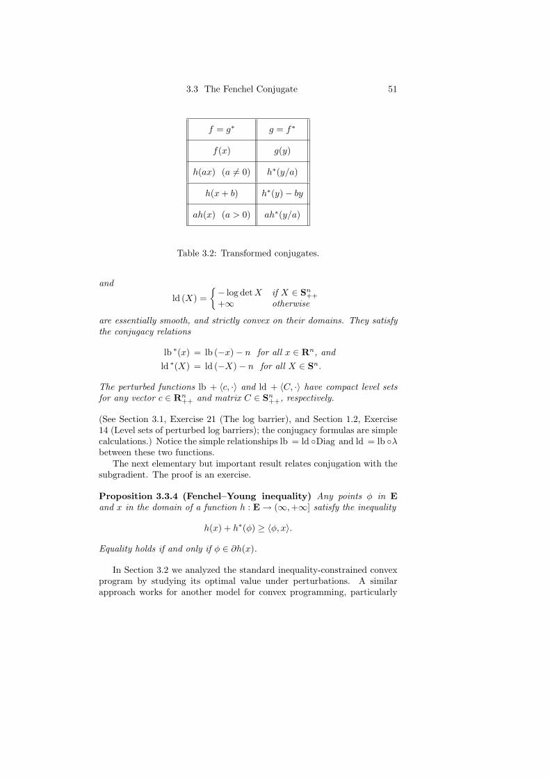
3.3 The Fenchel Conjugate 51
f = g∗ g = f∗
f(x) g(y)
h(ax) (a 6= 0) h∗(y/a)
h(x + b) h∗(y)− by
ah(x) (a > 0) ah∗(y/a)
Table 3.2: Transformed conjugates.
and
ld (X) =− log det X if X ∈ Sn
++
+∞ otherwise
are essentially smooth, and strictly convex on their domains. They satisfythe conjugacy relations
lb ∗(x) = lb (−x)− n for all x ∈ Rn, andld ∗(X) = ld (−X)− n for all X ∈ Sn.
The perturbed functions lb + 〈c, ·〉 and ld + 〈C, ·〉 have compact level setsfor any vector c ∈ Rn
++ and matrix C ∈ Sn++, respectively.
(See Section 3.1, Exercise 21 (The log barrier), and Section 1.2, Exercise14 (Level sets of perturbed log barriers); the conjugacy formulas are simplecalculations.) Notice the simple relationships lb = ld Diag and ld = lb λbetween these two functions.
The next elementary but important result relates conjugation with thesubgradient. The proof is an exercise.
Proposition 3.3.4 (Fenchel–Young inequality) Any points φ in Eand x in the domain of a function h : E → (∞, +∞] satisfy the inequality
h(x) + h∗(φ) ≥ 〈φ, x〉.
Equality holds if and only if φ ∈ ∂h(x).
In Section 3.2 we analyzed the standard inequality-constrained convexprogram by studying its optimal value under perturbations. A similarapproach works for another model for convex programming, particularly

52 3. Fenchel Duality
suited to problems with linear constraints. An interesting byproduct is aconvex analogue of the chain rule for differentiable functions,
∇(f + g A)(x) = ∇f(x) + A∗∇g(Ax)
(for a linear map A). When A is the identity map we obtain a sum rule.In this section we fix a Euclidean space Y. We denote the set of points
where a function g : Y → [−∞, +∞] is finite and continuous by cont g.
Theorem 3.3.5 (Fenchel duality and convex calculus) For givenfunctions f : E → (∞, +∞] and g : Y → (∞, +∞] and a linear mapA : E → Y, let p, d ∈ [−∞,+∞] be primal and dual values defined, respec-tively, by the Fenchel problems
p = infx∈E
f(x) + g(Ax) (3.3.6)
d = supφ∈Y
−f∗(A∗φ)− g∗(−φ). (3.3.7)
These values satisfy the weak duality inequality p ≥ d. If, furthermore,f and g are convex and satisfy the condition
0 ∈ core (dom g −Adom f) (3.3.8)
or the stronger condition
Adom f ∩ cont g 6= ∅ (3.3.9)
then the values are equal (p = d), and the supremum in the dual problem(3.3.7) is attained if finite.
At any point x in E, the calculus rule
∂(f + g A)(x) ⊃ ∂f(x) + A∗∂g(Ax) (3.3.10)
holds, with equality if f and g are convex and either condition (3.3.8) or(3.3.9) holds.
Proof. The weak duality inequality follows immediately from the Fenchel–Young inequality (3.3.4). To prove equality we define an optimal valuefunction h : Y → [−∞, +∞] by
h(u) = infx∈E
f(x) + g(Ax + u).
It is easy to check h is convex and dom h = dom g − Adom f . If p is −∞there is nothing to prove, while if condition (3.3.8) holds and p is finite
3.3 The Fenchel Conjugate 53
then Lemma 3.2.6 and the Max formula (3.1.8) show there is a subgradient−φ ∈ ∂h(0). Hence we deduce, for all u in Y and x in E, the inequalities
h(0) ≤ h(u) + 〈φ, u〉≤ f(x) + g(Ax + u) + 〈φ, u〉= f(x)− 〈A∗φ, x〉+ g(Ax + u)− 〈−φ,Ax + u〉.
Taking the infimum over all points u, and then over all points x, gives theinequalities
h(0) ≤ −f∗(A∗φ)− g∗(−φ) ≤ d ≤ p = h(0).
Thus φ attains the supremum in problem (3.3.7), and p = d. An easyexercise shows that condition (3.3.9) implies condition (3.3.8). The proof ofthe calculus rule in the second part of the theorem is a simple consequenceof the first part (Exercise 9). 2
The case of the Fenchel theorem above, when the function g is simplythe indicator function of a point, gives the following particularly elegantand useful corollary.
Corollary 3.3.11 (Fenchel duality for linear constraints) Given anyfunction f : E → (∞, +∞], any linear map A : E → Y, and any elementb of Y, the weak duality inequality
infx∈E
f(x) |Ax = b ≥ supφ∈Y
〈b, φ〉 − f∗(A∗φ)
holds. If f is convex and b belongs to core (Adom f) then equality holds,and the supremum is attained when finite.
A pretty application of the Fenchel duality circle of ideas is the calcu-lation of polar cones. The (negative) polar cone of the set K ⊂ E is theconvex cone
K− = φ ∈ E | 〈φ, x〉 ≤ 0 for all x ∈ K,
and the cone K−− is called the bipolar. A particularly important exampleof the polar cone is the normal cone to a convex set C ⊂ E at a point x inC, since NC(x) = (C − x)−.
We use the following two examples extensively; the proofs are simpleexercises.
Proposition 3.3.12 (Self-dual cones)
(Rn+)− = −Rn
+ and (Sn+)− = −Sn
+.

54 3. Fenchel Duality
The next result shows how the calculus rules above can be used to derivegeometric consequences.
Corollary 3.3.13 (Krein–Rutman polar cone calculus) Any conesH ⊂ Y and K ⊂ E and linear map A : E → Y satisfy
(K ∩A−1H)− ⊃ A∗H− + K−.
Equality holds if H and K are convex and satisfy H − AK = Y (or inparticular AK ∩ intH 6= ∅).
Proof. Rephrasing the definition of the polar cone shows that for anycone K ⊂ E, the polar cone K− is just ∂δK(0). The result now follows bythe Fenchel theorem above. 2
The polarity operation arises naturally from Fenchel conjugation, sincefor any cone K ⊂ E we have δK− = δ∗K , whence δK−− = δ∗∗K . The nextresult, which is an elementary application of the Basic separation theo-rem (2.1.6), leads naturally into the development of the next chapter byidentifying K−− as the closed convex cone generated by K.
Theorem 3.3.14 (Bipolar cone) The bipolar cone of any nonempty setK ⊂ E is given by K−− = cl (conv (R+K)).
For example, we deduce immediately that the normal cone NC(x) to aconvex set C at a point x in C, and the (convex) tangent cone to C at xdefined by TC(x) = clR+(C − x), are polars of each other.
Exercise 20 outlines how to use these two results about cones to charac-terize pointed cones (those closed convex cones K satisfying K∩−K = 0).
Theorem 3.3.15 (Pointed cones) If K ⊂ E is a closed convex cone,then K is pointed if and only if there is an element y of E for which theset
C = x ∈ K | 〈x, y〉 = 1is compact and generates K (that is, K = R+C).
Exercises and Commentary
The conjugation operation has been closely associated with the namesof Legendre, Moreau, and Rockafellar, as well as Fenchel; see [167, 70].Fenchel’s original work is [76]. A good reference for properties of convexcones is [151]; see also [20]. The log barriers of Proposition 3.3.3 play a keyrole in interior point methods for linear and semidefinite programming—see, for example, [148]. The self-duality of the positive semidefinite cone is
3.3 The Fenchel Conjugate 55
due to Fejer [99]. Hahn–Banach extension (Exercise 13(e)) is a key tech-nique in functional analysis; see, for example, [98]. Exercise 21 (Ordersubgradients) is aimed at multicriteria optimization; a good reference is[176]. Our approach may be found, for example, in [20]. The last threefunctions g in Table 3.1 are respectively known as the Boltzmann–Shannon,Fermi–Dirac, and Bose–Einstein entropies.
1. For each of the functions f in Table 3.1, check the calculation of f∗
and check f = f∗∗.
2. (Quadratics) For all matrices A in Sn++, prove the function x ∈
Rn 7→ xT Ax/2 is convex and calculate its conjugate. Use the order-reversing property of the conjugacy operation to prove
A º B ⇔ B−1 º A−1 for A and B in Sn++.
3. Verify the conjugates of the log barriers lb and ld claimed in Propo-sition 3.3.3.
4. ∗ (Self-conjugacy) Consider functions f : E → (∞, +∞].
(a) Prove f = f∗ if and only if f(x) = ‖x‖2/2 for all points x in E.(b) Find two distinct functions f satisfying f(−x) = f∗(x) for all
points x in E.
5. ∗ (Support functions) The conjugate of the indicator function ofa nonempty set C ⊂ E, namely δ∗C : E → (∞,+∞], is called thesupport function of C. Calculate it for the following sets:
(a) the halfspace x | 〈a, x〉 ≤ b for 0 6= a ∈ E and b ∈ R(b) the unit ball B
(c) x ∈ Rn+ | ‖x‖ ≤ 1
(d) the polytope conv a1, a2, . . . , am for given points a1, a2, . . . , am
in E(e) a cone K
(f) the epigraph of a convex function f : E → (∞,+∞](g) the subdifferential ∂f(x), where the function f : E → (∞, +∞]
is convex and the point x lies in core (dom f)(h) Y ∈ Sn
+ | trY = 16. Calculate the conjugate and biconjugate of the function
f(x1, x2) =
x21
2x2+ x2 log x2 − x2 if x2 > 0
0 if x1 = x2 = 0+∞ otherwise.

56 3. Fenchel Duality
7. ∗∗ (Maximum entropy example)
(a) Prove the function g defined by (3.3.1) is convex.
(b) For any point y in Rm+1, prove
g∗(y) = supx∈Rm+1
∑
i
(xi〈ai, y〉 − exp∗(xi))∣∣∣
∑
i
xi = 1
.
(c) Apply Exercise 27 in Section 3.1 to deduce the conjugacy for-mula (3.3.2).
(d) Compute the conjugate of the function of x ∈ Rm+1, ∑
i exp∗(xi) if∑
i xi = 1+∞ otherwise.
8. Prove the Fenchel–Young inequality.
9. ∗ (Fenchel duality and convex calculus) Fill in the details forthe proof of Theorem 3.3.5 as follows.
(a) Prove the weak duality inequality.
(b) Prove the inclusion (3.3.10).
Now assume f and g are convex.
(c) Prove the function h defined in the proof is convex with domaindom g −Adom f .
(d) Prove the implication (3.3.9) ⇒ (3.3.8).
Finally, assume in addition that condition (3.3.8) holds.
(e) Suppose φ ∈ ∂(f + g A)(x). Use the first part of the theoremand the fact that x is an optimal solution of the problem
infx∈E
(f(x)− 〈φ, x〉) + g(Ax)
to deduce equality in part (b).
(f) Prove points x ∈ E and φ ∈ Y are optimal for problems (3.3.6)and (3.3.7), respectively, if and only if they satisfy the conditionsA∗φ ∈ ∂f(x) and −φ ∈ ∂g(Ax).
10. (Normals to an intersection) If the point x lies in two convexsubsets C and D of E satisfying 0 ∈ core (C − D) (or in particularC ∩ intD 6= ∅), use Section 3.1, Exercise 4 (Subgradients and normalcones) to prove
NC∩D(x) = NC(x) + ND(x).

3.3 The Fenchel Conjugate 57
11. ∗ (Failure of convex calculus)
(a) Find convex functions f, g : R → (∞,+∞] with
∂f(0) + ∂g(0) 6= ∂(f + g)(0).
(Hint: Section 3.1, Exercise 5.)
(b) Find a convex function g : R2 → (∞, +∞] and a linear mapA : R → R2 with A∗∂g(0) 6= ∂(g A)(0).
12. ∗ (Infimal convolution) If the functions f, g : E → (−∞, +∞] areconvex, we define the infimal convolution f ¯ g : E → [−∞, +∞] by
(f ¯ g)(y) = infxf(x) + g(y − x).
(a) Prove f ¯ g is convex. (On the other hand, if g is concave proveso is f ¯ g.)
(b) Prove (f ¯ g)∗ = f∗ + g∗.
(c) If dom f ∩ cont g 6= ∅, prove (f + g)∗ = f∗ ¯ g∗.
(d) Given a nonempty set C ⊂ E, define the distance function by
dC(x) = infy∈C
‖x− y‖.
(i) Prove d2C is a difference of convex functions, by observing
(dC(x))2 =‖x‖2
2−
(‖ · ‖22
+ δC
)∗(x).
Now suppose C is convex.
(ii) Prove dC is convex and d∗C = δB + δ∗C .(iii) For x in C prove ∂dC(x) = B ∩NC(x).(iv) If C is closed and x 6∈ C, prove
∇dC(x) = dC(x)−1(x− PC(x)),
where PC(x) is the nearest point to x in C.(v) If C is closed, prove
∇d2C
2(x) = x− PC(x)
for all points x.
58 3. Fenchel Duality
(e) Define the Lambert W -function W : R+ → R+ as the inverse ofy ∈ R+ 7→ yey. Prove the conjugate of the function
x ∈ R 7→ exp∗(x) +x2
2
is the function
y ∈ R 7→ W (ey) +(W (ey))2
2.
13. ∗ (Applications of Fenchel duality)
(a) (Sandwich theorem) Let the functions f : E → (∞, +∞]and g : Y → (∞,+∞] be convex and the map A : E → Y belinear. Suppose f ≥ −g A and 0 ∈ core (dom g − Adom f)(or Adom f ∩ cont g 6= ∅). Prove there is an affine functionα : E → R satisfying f ≥ α ≥ −g A.
(b) Interpret the Sandwich theorem geometrically in the case whenA is the identity.
(c) (Pshenichnii–Rockafellar conditions [159]) If the convexset C in E satisfies the condition C∩cont f 6= ∅ (or the conditionintC∩dom f 6= ∅), and if f is bounded below on C, use part (a)to prove there is an affine function α ≤ f with infC f = infC α.Deduce that a point x minimizes f on C if and only if it satisfies0 ∈ ∂f(x) + NC(x).
(d) Apply part (c) to the following two cases:
(i) C a single point x0 ⊂ E(ii) C a polyhedron x |Ax ≤ b, where b ∈ Rn = Y
(e) (Hahn–Banach extension) If the function f : E → R iseverywhere finite and sublinear, and for some linear subspaceL of E the function h : L → R is linear and dominated by f(in other words f ≥ h on L), prove there is a linear functionα : E → R, dominated by f , which agrees with h on L.
14. Fill in the details of the proof of the Krein–Rutman calculus (3.3.13).
15. ∗ (Bipolar theorem) For any nonempty set K ⊂ E, prove theset cl (conv (R+K)) is the smallest closed convex cone containing K.Deduce Theorem 3.3.14 (Bipolar cones).
16. ∗ (Sums of closed cones)
(a) Prove that any cones H,K ⊂ E satisfy (H + K)− = H− ∩K−.
3.3 The Fenchel Conjugate 59
(b) Deduce that if H and K are closed convex cones then they satisfy(H ∩K)− = cl (H− + K−), and prove that the closure can beomitted under the condition K ∩ intH 6= ∅.
In R3, define sets
H = x | x21 + x2
2 ≤ x23, x3 ≤ 0 and
K = x | x2 = −x3.
(c) Prove H and K are closed convex cones.
(d) Calculate the polar cones H−, K−, and (H ∩K)−.
(e) Prove (1, 1, 1) ∈ (H ∩K)− \ (H− + K−), and deduce that thesum of two closed convex cones is not necessarily closed.
17. ∗ (Subdifferential of a max-function) With the notation of Sec-tion 3.2, Exercise 13, suppose
dom gj ∩⋂
i∈I\jcont gi 6= ∅
for some index j in I. Prove
∂(maxi
gi)(x) = conv⋃
i∈I
∂gi(x).
18. ∗ (Order convexity) Given a Euclidean space Y and a closed convexcone S ⊂ Y, we write u ≤S v for points u and v in Y if v − u lies inS.
(a) Identify the partial order ≤S in the following cases:
(i) S = 0(ii) S = Y(iii) Y = Rn and S = Rn
+
Given a convex set C ⊂ E, we say a function F : C → Y is S-convexif it satisfies
F (λx + µz) ≤S λF (x) + µF (z)
for all points x and z in E and nonnegative reals λ and µ satisfyingλ + µ = 1. If, furthermore, C is a cone and this inequality holds forall λ and µ in R+ then we say F is S-sublinear.
(b) Identify S-convexity in the cases listed in part (a).
(c) Prove F is S-convex if and only if the function 〈φ, F (·)〉 is convexfor all elements φ of −S−.

60 3. Fenchel Duality
(d) Prove the following functions are Sn+-convex:
(i) X ∈ Sn 7→ X2
(ii) X ∈ Sn++ 7→ X−1
(iii) X ∈ Sn+ 7→ −X1/2
Hint: Use Exercise 25 in Section 3.1.
(e) Prove the function X ∈ S2 7→ X4 is not S2+-convex. Hint:
Consider the matrices[
4 22 1
]and
[4 00 8
].
19. (Order convexity of inversion) For any matrix A in Sn++, define
a function qA : Rn → R by qA(x) = xT Ax/2.
(a) Prove q∗A = qA−1 .
(b) For any other matrix B in Sn++, prove 2(qA ¯ qB) ≤ q(A+B)/2.
(See Exercise 12.)
(c) Deduce (A−1 + B−1)/2 º ((A + B)/2)−1.
20. ∗∗ (Pointed cones and bases) Consider a closed convex cone Kin E. A base for K is a convex set C with 0 6∈ clC and K = R+C.Using Exercise 16, prove the following properties are equivalent byshowing the implications
(a) ⇒ (b) ⇒ (c) ⇒ (d) ⇒ (e) ⇒ (f) ⇒ (a).
(a) K is pointed.
(b) cl (K− −K−) = E.
(c) K− −K− = E.
(d) K− has nonempty interior. (Here you may use the fact that K−
has nonempty relative interior—see Section 1.1, Exercise 13.)
(e) There exists a vector y in E and real ε > 0 with 〈y, x〉 ≥ ε‖x‖for all points x in K.
(f) K has a bounded base.
21. ∗∗ (Order-subgradients) This exercise uses the terminology of Ex-ercise 18, and we assume the cone S ⊂ Y is pointed: S ∩ −S = 0.An element y of Y is the S-infimum of a set D ⊂ Y (writteny = infS D) if the conditions
(i) D ⊂ y + S and
(ii) D ⊂ z + S for some z in Y implies y ∈ z + S

3.3 The Fenchel Conjugate 61
both hold.
(a) Verify that this notion corresponds to the usual infimum whenY = R and S = R+.
(b) Prove every subset of Y has at most one S-infimum.
(c) Prove decreasing sequences in S converge:
x0 ≥S x1 ≥S x2 . . . ≥S 0
implies limn xn exists and equals infS(xn). (Hint: Prove firstthat S ∩ (x0 − S) is compact using Section 1.1, Exercise 6 (Re-cession cones).)
An S-subgradient of F at a point x in C is a linear map T : E → Ysatisfying
T (z − x) ≤S F (z)− F (x) for all z in C.
The set of S-subgradients is denoted ∂SF (x). Suppose now x ∈coreC. Generalize the arguments of Section 3.1 in the following steps.
(d) For any direction h in E, prove
∇SF (x; h) = infSt−1(F (x + th)− F (x)) | t > 0, x + th ∈ C
exists and, as a function of h, is S-sublinear.
(e) For any S-subgradient T ∈ ∂SF (x) and direction h ∈ E, proveTh ≤S ∇SF (x;h).
(f) Given h in E, prove there exists T in ∂SF (x) satisfying Th =∇SF (x; h). Deduce the max formula
∇SF (x; h) = maxTh | T ∈ ∂SF (x)
and, in particular, that ∂SF (x) is nonempty. (You should inter-pret the “max” in the formula.)
(g) The function F is Gateaux differentiable at x (with derivativethe linear map ∇F (x) : E → Y) if
limt→0
t−1(F (x + th)− F (x)) = (∇F (x))h
holds for all h in E. Prove this is the case if and only if ∂SF (x)is a singleton.
Now fix an element φ of −int (S−).
(h) Prove 〈φ, F (·)〉′(x; h) = 〈φ,∇SF (x; h)〉.

62 3. Fenchel Duality
(i) Prove F is Gateaux differentiable at x if and only if 〈φ, F (·)〉 islikewise.
22. ∗∗ (Linearly constrained examples) Prove Corollary 3.3.11 (Fen-chel duality for linear constraints). Deduce duality theorems for thefollowing problems.
(a) Separable problems
inf n∑
i=1
p(xi)∣∣∣ Ax = b
,
where the map A : Rn → Rm is linear, b ∈ Rm, and the functionp : R → (∞, +∞] is convex, defined as follows:
(i) (Nearest points in polyhedrons) p(t) = t2/2 with do-main R+.
(ii) (Analytic center) p(t) = − log t with domain R++.(iii) (Maximum entropy) p = exp∗.
What happens if the objective function is replaced by∑
i pi(xi)?
(b) The BFGS update problem in Section 2.1, Exercise 13.
(c) The DAD problem in Section 3.1, Exercise 28.
(d) Example (3.3.1).
23. ∗ (Linear inequalities) What does Corollary 3.3.11 (Fenchel dualityfor linear constraints) become if we replace the constraint Ax = b byAx ∈ b + K where K ⊂ Y is a convex cone? Write down the dualproblem for Section 3.2, Exercise 2, part (a), solve it, and verify theduality theorem.
24. (Symmetric Fenchel duality) For functions f, g : E → [−∞,+∞],define the concave conjugate g∗ : E → [−∞,+∞] by
g∗(φ) = infx∈E
〈φ, x〉 − g(x).
Proveinf(f − g) ≥ sup(g∗ − f∗),
with equality if f is convex, g is concave, and
0 ∈ core (dom f − dom (−g)).

3.3 The Fenchel Conjugate 63
25. ∗∗ (Divergence bounds [135])
(a) Prove the function
t ∈ R 7→ 2(2 + t)(exp∗ t + 1)− 3(t− 1)2
is convex and is minimized when t = 1.
(b) For v in R++ and u in R+, deduce the inequality
3(u− v)2 ≤ 2(u + 2v)(u log
(u
v
)− u + v
).
Now suppose the vector p in Rn++ satisfies
∑n1 pi = 1.
(c) If the vector q ∈ Rn++ satisfies
∑n1 qi = 1, use the Cauchy–
Schwarz inequality to prove the inequality
( n∑1
|pi − qi|)2
≤ 3n∑1
(pi − qi)2
pi + 2qi,
and deduce the inequality
n∑1
pi log(pi
qi
)≥ 1
2
( n∑1
|pi − qi|)2
.
(d) Hence show the inequality
log n +n∑1
pi log pi ≥ 12
( n∑1
∣∣∣pi − 1n
∣∣∣)2
.
(e) Use convexity to prove the inequality
n∑1
pi log pi ≤ logn∑1
p2i .
(f) Deduce the bound
log n +n∑1
pi log pi ≤ max pi
min pi− 1.

64 3. Fenchel Duality
Chapter 4
Convex Analysis
4.1 Continuity of Convex Functions
We have already seen that linear functions are always continuous. Moregenerally, a remarkable feature of convex functions on E is that they mustbe continuous on the interior of their domains. Part of the surprise is thatan algebraic/geometric assumption (convexity) leads to a topological con-clusion (continuity). It is this powerful fact that guarantees the usefulnessof regularity conditions like Adom f ∩ cont g 6= ∅ (3.3.9), which we studiedin the previous section.
Clearly an arbitrary function f is bounded above on some neighbour-hood of any point in cont f . For convex functions the converse is also true,and in a rather strong sense, needing the following definition. For a realL ≥ 0, we say that a function f : E → (∞,+∞] is Lipschitz (with constantL) on a subset C of dom f if |f(x) − f(y)| ≤ L‖x − y‖ for any points xand y in C. If f is Lipschitz on a neighbourhood of a point z then we saythat f is locally Lipschitz around z. If Y is another Euclidean space wemake analogous definitions for functions F : E → Y, with ‖F (x) − F (y)‖replacing |f(x)− f(y)|.
Theorem 4.1.1 (Local boundedness) Let f : E → (∞, +∞] be a con-vex function. Then f is locally Lipschitz around a point z in its domain ifand only if it is bounded above on a neighbourhood of z.
Proof. One direction is clear, so let us without loss of generality takez = 0, f(0) = 0, and suppose f ≤ 1 on 2B; we shall deduce f is Lipschitzon B.
Notice first the bound f ≥ −1 on 2B, since convexity implies f(−x) ≥−f(x) on 2B. Now for any distinct points x and y in B, define α = ‖y−x‖and fix a point w = y + α−1(y − x), which lies in 2B. By convexity we
65
66 4. Convex Analysis
obtain
f(y)− f(x) ≤ 11 + α
f(x) +α
1 + αf(w)− f(x) ≤ 2α
1 + α≤ 2‖y − x‖,
and the result now follows, since x and y may be interchanged. 2
This result makes it easy to identify the set of points at which a convexfunction on E is continuous. First we prove a key lemma.
Lemma 4.1.2 Let ∆ be the simplex x ∈ Rn+ |
∑xi ≤ 1. If the function
g : ∆ → R is convex then it is continuous on int∆.
Proof. By the above result, we just need to show g is bounded above on∆. But any point x in ∆ satisfies
g(x) = g( n∑
1
xiei + (1−∑
xi)0)≤
n∑1
xig(ei) + (1−∑xi)g(0)
≤ maxg(e1), g(e2), . . . , g(en), g(0)(where e1, e2, . . . , en is the standard basis in Rn). 2
Theorem 4.1.3 (Convexity and continuity) Let f : E → (∞,+∞] bea convex function. Then f is continuous (in fact locally Lipschitz) on theinterior of its domain.
Proof. We lose no generality if we restrict ourselves to the case E = Rn.For any point x in int (dom f) we can choose a neighbourhood of x in dom fthat is a scaled down, translated copy of the simplex (since the simplex isbounded with nonempty interior). The proof of the preceding lemma nowshows f is bounded above on a neighbourhood of x, and the result followsby Theorem 4.1.1 (Local boundedness). 2
Since it is easy to see that if the convex function f is locally Lipschitzaround a point x in int (dom f) with constant L then ∂f(x) ⊂ LB, wecan also conclude that ∂f(x) is a nonempty compact convex set. Further-more, this result allows us to conclude quickly that “all norms on E areequivalent” (see Exercise 2).
We have seen that for a convex function f , the two sets cont f andint (dom f) are identical. By contrast, our algebraic approach to the ex-istence of subgradients involved core (dom f). It transpires that this isthe same set. To see this we introduce the idea of the gauge functionγC : E → (∞, +∞] associated with a nonempty set C in E:
γC(x) = infλ ∈ R+ | x ∈ λC.It is easy to check γC is sublinear (and in particular convex) when C isconvex. Notice γB = ‖ · ‖.
4.1 Continuity of Convex Functions 67
Theorem 4.1.4 (Core and interior) The core and the interior of anyconvex set in E are identical and convex.
Proof. Any convex set C ⊂ E clearly satisfies intC ⊂ core C. If wesuppose, without loss of generality, 0 ∈ core C, then γC is everywherefinite, and hence continuous by the previous result. We claim
intC = x | γC(x) < 1.
To see this, observe that the right hand side is contained in C, and is openby continuity, and hence is contained in intC. The reverse inclusion is easy,and we deduce intC is convex. Finally, since γC(0) = 0, we see 0 ∈ intC,which completes the proof. 2
The conjugate of the gauge function γC is the indicator function of aset C ⊂ E defined by
C = φ ∈ E | 〈φ, x〉 ≤ 1 for all x ∈ C.
We call C the polar set for C. Clearly it is a closed convex set containing0, and when C is a cone it coincides with the polar cone C−. The followingresult therefore generalizes the Bipolar cone theorem (3.3.14).
Theorem 4.1.5 (Bipolar set) The bipolar set of any subset C of E isgiven by
C = cl (conv (C ∪ 0)).
The ideas of polarity and separating hyperplanes are intimately related.The separation-based proof of the above result (Exercise 5) is a good ex-ample, as is the next theorem, whose proof is outlined in Exercise 6.
Theorem 4.1.6 (Supporting hyperplane) Suppose that the convex setC ⊂ E has nonempty interior and that the point x lies on the boundary ofC. Then there is a supporting hyperplane to C at x: there is a nonzeroelement a of E satisfying 〈a, x〉 ≥ 〈a, x〉 for all points x in C.
(The set x ∈ E | 〈a, x− x〉 = 0 is the supporting hyperplane.)
To end this section we use this result to prove a remarkable theoremof Minkowski describing an extremal representation of finite-dimensionalcompact convex sets. An extreme point of a convex set C ⊂ E is a point xin C whose complement C \ x is convex. We denote the set of extremepoints by ext C. We start with another exercise.
Lemma 4.1.7 Given a supporting hyperplane H of a convex set C ⊂ E,any extreme point of C ∩H is also an extreme point of C.
68 4. Convex Analysis
Our proof of Minkowski’s theorem depends on two facts: first, anyconvex set that spans E and contains the origin has nonempty interior (seeSection 1.1, Exercise 13(b)); second, we can define the dimension of a setC ⊂ E (written dim C) as the dimension of span (C−x) for any point x inC (see Section 1.1, Exercise 12 (Affine sets)).
Theorem 4.1.8 (Minkowski) Any compact convex set C ⊂ E is the con-vex hull of its extreme points.
Proof. Our proof is by induction on dimC; clearly the result holds whendim C = 0. Assume the result holds for all sets of dimension less thandim C. We will deduce it for the set C.
By translating C and redefining E, we can assume 0 ∈ C and span C =E. Thus C has nonempty interior.
Given any point x in bdC, the Supporting hyperplane theorem (4.1.6)shows C has a supporting hyperplane H at x. By the induction hypothesisapplied to the set C ∩H we deduce, using Lemma 4.1.7,
x ∈ conv (ext (C ∩H)) ⊂ conv (ext C).
Thus we have proved bdC ⊂ conv (ext C), so conv (bd C) ⊂ conv (ext C).But since C is compact it is easy to see conv (bd C) = C, and the resultnow follows. 2
Exercises and Commentary
An easy introduction to convex analysis in finite dimensions is [181]. Theapproach we adopt here (and in the exercises) extends easily to infinitedimensions; see [98, 131, 153]. The Lipschitz condition was introducedin [129]. Minkowski’s theorem first appeared in [141, 142]. The Openmapping theorem (Exercise 9) is another fundamental tool of functionalanalysis [98]. For recent references on Pareto minimization (Exercise 12),see [44].
1. ∗ (Points of continuity) Suppose the function f : E → (∞,+∞] isconvex.
(a) Use the Local boundedness theorem (4.1.1) to prove that f iscontinuous and finite at x if and only if it minorizes a functiong : E → (∞, +∞] which is continuous and finite at x.
(b) Suppose f is continuous at some point y in dom f . Use part(a) to prove directly that f is continuous at any point z incore (dom f). (Hint: Pick a point u in dom f such that z =δy + (1 − δ)u for some real δ ∈ (0, 1); now observe that thefunction
x ∈ E 7→ δ−1(f(δx + (1− δ)u)− (1− δ)f(u))

4.1 Continuity of Convex Functions 69
minorizes f .)
(c) Prove that f is continuous at a point x in dom f if and only if
(x, f(x) + ε) ∈ int (epi f)
for some (all) real ε > 0.
(d) Assuming 0 ∈ cont f , prove f∗ has bounded level sets. Deducethat the function X ∈ Sn 7→ 〈C, X〉+ ld (X) has compact levelsets for any matrix C in Sn
++.
(e) Assuming x ∈ cont f , prove ∂f(x) is a nonempty compact con-vex set.
2. (Equivalent norms) A norm is a sublinear function |‖·|‖ : E → R+
that satisfies |‖x|‖ = |‖ − x|‖ > 0 for all nonzero points x in E. Byconsidering the function |‖ · |‖ on the standard unit ball B, prove anynorm |‖ · |‖ is equivalent to the Euclidean norm ‖ · ‖: that is, thereare constants K ≥ k > 0 with k‖x‖ ≤ |‖x|‖ ≤ K‖x‖ for all x.
3. (Examples of polars) Calculate the polars of the following sets:
(a) conv(B ∪ (1, 1), (−1,−1)) ⊂ R2.
(b)
(x, y) ∈ R2∣∣∣ y ≥ b +
x2
2
(b ∈ R).
4. (Polar sets and cones) Suppose the set C ⊂ E is closed, convex,and contains 0. Prove the convex cones in E×R
clR+(C × 1) and clR+(C × −1)
are mutually polar.
5. ∗ (Polar sets) Suppose C is a nonempty subset of E.
(a) Prove γ∗C = δC .
(b) Prove C is a closed convex set containing 0.
(c) Prove C ⊂ C.
(d) If C is a cone, prove C = C−.
(e) For a subset D of E, prove C ⊂ D implies D ⊂ C.
(f) Prove C is bounded if and only if 0 ∈ intC.
(g) For any closed halfspace H ⊂ E containing 0, prove H = H.
(h) Prove Theorem 4.1.5 (Bipolar set).
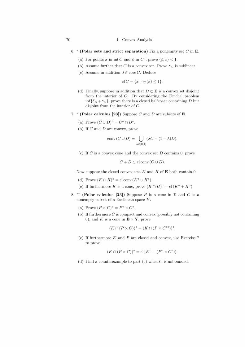
70 4. Convex Analysis
6. ∗ (Polar sets and strict separation) Fix a nonempty set C in E.
(a) For points x in intC and φ in C, prove 〈φ, x〉 < 1.
(b) Assume further that C is a convex set. Prove γC is sublinear.
(c) Assume in addition 0 ∈ coreC. Deduce
cl C = x | γC(x) ≤ 1.
(d) Finally, suppose in addition that D ⊂ E is a convex set disjointfrom the interior of C. By considering the Fenchel probleminfδD +γC, prove there is a closed halfspace containing D butdisjoint from the interior of C.
7. ∗ (Polar calculus [23]) Suppose C and D are subsets of E.
(a) Prove (C ∪D) = C ∩D.
(b) If C and D are convex, prove
conv (C ∪D) =⋃
λ∈[0,1]
(λC + (1− λ)D).
(c) If C is a convex cone and the convex set D contains 0, prove
C + D ⊂ cl conv (C ∪D).
Now suppose the closed convex sets K and H of E both contain 0.
(d) Prove (K ∩H) = cl conv (K ∪H).
(e) If furthermore K is a cone, prove (K ∩H) = cl (K + H).
8. ∗∗ (Polar calculus [23]) Suppose P is a cone in E and C is anonempty subset of a Euclidean space Y.
(a) Prove (P × C) = P × C.
(b) If furthermore C is compact and convex (possibly not containing0), and K is a cone in E×Y, prove
(K ∩ (P × C)) = (K ∩ (P × C)).
(c) If furthermore K and P are closed and convex, use Exercise 7to prove
(K ∩ (P × C)) = cl (K + (P × C)).
(d) Find a counterexample to part (c) when C is unbounded.

4.1 Continuity of Convex Functions 71
9. ∗ (Open mapping theorem) Suppose the linear map A : E → Yis surjective.
(a) Prove any set C ⊂ E satisfies Acore C ⊂ coreAC.(b) Deduce A is an open map: that is, the image of any open set is
open.(c) Prove another condition ensuring condition (3.3.8) in the Fenchel
theorem is that there is a point x in int (dom f) with Ax in dom gand A is surjective. Prove similarly that a sufficient conditionfor Fenchel duality with linear constraints (Corollary 3.3.11) tohold is A surjective and b ∈ A(int (dom f)).
(d) Deduce that any cones H ⊂ Y and K ⊂ E, and any surjectivelinear map A : E → Y satisfy (K ∩ A−1H)− = A∗H− + K−,providing H ∩A(intK) 6= ∅.
10. ∗ (Conical absorption)
(a) If the set A ⊂ E is convex, the set C ⊂ E is bounded, andR+A = E, prove there exists a real δ > 0 such that δC ⊂ A.
Now define two sets in S2+ by
A =[
y xx z
]∈ S2
+
∣∣∣∣ |x| ≤ y2/3
, and
C = X ∈ S2+ | tr X ≤ 1.
(b) Prove that both A and C are closed, convex, and contain 0, andthat C is bounded.
(c) Prove R+A = S2+ = R+C.
(d) Prove there is no real δ > 0 such that δC ⊂ A.
11. (Holder’s inequality) This question develops an alternative ap-proach to the theory of the p-norm ‖ · ‖p defined in Section 2.3, Ex-ercise 6.
(a) Prove p−1‖x‖pp is a convex function, and deduce the set
Bp = x | ‖x‖p ≤ 1is convex.
(b) Prove the gauge function γBp(·) is exactly ‖·‖p, and deduce ‖·‖p
is convex.(c) Use the Fenchel–Young inequality (3.3.4) to prove that any vec-
tors x and φ in Rn satisfy the inequality
p−1‖x‖pp + q−1‖φ‖q
q ≥ 〈φ, x〉.
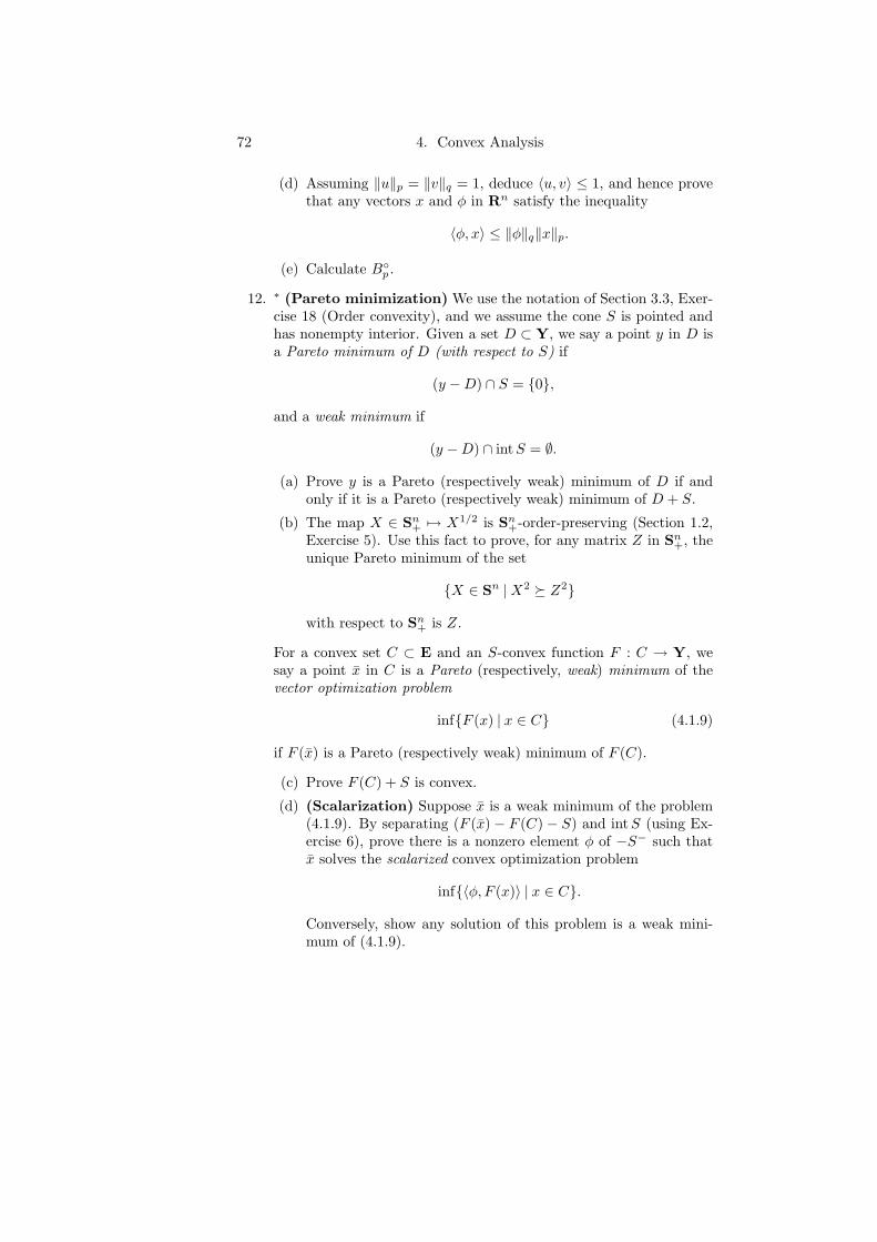
72 4. Convex Analysis
(d) Assuming ‖u‖p = ‖v‖q = 1, deduce 〈u, v〉 ≤ 1, and hence provethat any vectors x and φ in Rn satisfy the inequality
〈φ, x〉 ≤ ‖φ‖q‖x‖p.
(e) Calculate Bp .
12. ∗ (Pareto minimization) We use the notation of Section 3.3, Exer-cise 18 (Order convexity), and we assume the cone S is pointed andhas nonempty interior. Given a set D ⊂ Y, we say a point y in D isa Pareto minimum of D (with respect to S) if
(y −D) ∩ S = 0,
and a weak minimum if
(y −D) ∩ intS = ∅.
(a) Prove y is a Pareto (respectively weak) minimum of D if andonly if it is a Pareto (respectively weak) minimum of D + S.
(b) The map X ∈ Sn+ 7→ X1/2 is Sn
+-order-preserving (Section 1.2,Exercise 5). Use this fact to prove, for any matrix Z in Sn
+, theunique Pareto minimum of the set
X ∈ Sn |X2 º Z2
with respect to Sn+ is Z.
For a convex set C ⊂ E and an S-convex function F : C → Y, wesay a point x in C is a Pareto (respectively, weak) minimum of thevector optimization problem
infF (x) | x ∈ C (4.1.9)
if F (x) is a Pareto (respectively weak) minimum of F (C).
(c) Prove F (C) + S is convex.
(d) (Scalarization) Suppose x is a weak minimum of the problem(4.1.9). By separating (F (x)− F (C)− S) and intS (using Ex-ercise 6), prove there is a nonzero element φ of −S− such thatx solves the scalarized convex optimization problem
inf〈φ, F (x)〉 | x ∈ C.
Conversely, show any solution of this problem is a weak mini-mum of (4.1.9).
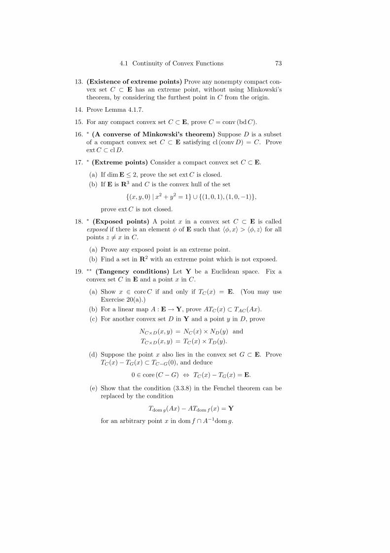
4.1 Continuity of Convex Functions 73
13. (Existence of extreme points) Prove any nonempty compact con-vex set C ⊂ E has an extreme point, without using Minkowski’stheorem, by considering the furthest point in C from the origin.
14. Prove Lemma 4.1.7.
15. For any compact convex set C ⊂ E, prove C = conv (bd C).
16. ∗ (A converse of Minkowski’s theorem) Suppose D is a subsetof a compact convex set C ⊂ E satisfying cl (convD) = C. Proveext C ⊂ clD.
17. ∗ (Extreme points) Consider a compact convex set C ⊂ E.
(a) If dimE ≤ 2, prove the set extC is closed.(b) If E is R3 and C is the convex hull of the set
(x, y, 0) | x2 + y2 = 1 ∪ (1, 0, 1), (1, 0,−1),prove ext C is not closed.
18. ∗ (Exposed points) A point x in a convex set C ⊂ E is calledexposed if there is an element φ of E such that 〈φ, x〉 > 〈φ, z〉 for allpoints z 6= x in C.
(a) Prove any exposed point is an extreme point.(b) Find a set in R2 with an extreme point which is not exposed.
19. ∗∗ (Tangency conditions) Let Y be a Euclidean space. Fix aconvex set C in E and a point x in C.
(a) Show x ∈ core C if and only if TC(x) = E. (You may useExercise 20(a).)
(b) For a linear map A : E → Y, prove ATC(x) ⊂ TAC(Ax).(c) For another convex set D in Y and a point y in D, prove
NC×D(x, y) = NC(x)×ND(y) andTC×D(x, y) = TC(x)× TD(y).
(d) Suppose the point x also lies in the convex set G ⊂ E. ProveTC(x)− TG(x) ⊂ TC−G(0), and deduce
0 ∈ core (C −G) ⇔ TC(x)− TG(x) = E.
(e) Show that the condition (3.3.8) in the Fenchel theorem can bereplaced by the condition
Tdom g(Ax)−ATdom f (x) = Y
for an arbitrary point x in dom f ∩A−1dom g.

74 4. Convex Analysis
20. ∗∗ (Properties of the relative interior) (We use Exercise 9 (Openmapping theorem), as well as Section 1.1, Exercise 13.)
(a) Let D be a nonempty convex set in E. Prove D is a linearsubspace if and only if clD is a linear subspace. (Hint: ri D 6= ∅.)
(b) For a point x in a convex set C ⊂ E, prove the following prop-erties are equivalent:
(i) x ∈ ri C.(ii) The tangent cone clR+(C − x) is a linear subspace.(iii) The normal cone NC(x) is a linear subspace.(iv) y ∈ NC(x) ⇒ −y ∈ NC(x).
(c) For a convex set C ⊂ E and a linear map A : E → Y, proveAri C ⊃ ri AC, and deduce
Ari C = ri AC.
(d) Suppose U and V are convex sets in E. Deduce
ri (U − V ) = ri U − ri V.
(e) Apply Section 3.1, Exercise 29 (Relativizing the Max formula)to conclude that the condition (3.3.8) in the Fenchel theorem(3.3.5) can be replaced by
ri (dom g) ∩Ari (dom f) 6= ∅.
(f) Suppose the function f : E → (∞,+∞] is bounded below onthe convex set C ⊂ E, and ri C ∩ ri (dom f) 6= ∅. Prove there isan affine function α ≤ f with infC f = infC α.
21. ∗∗ (Essential smoothness) For any convex function f and any pointx ∈ bd(dom f), prove ∂f(x) is either empty or unbounded. Deducethat a function is essentially smooth if and only if its subdifferentialis always singleton or empty.
22. ∗∗ (Birkhoff’s theorem [15]) We use the notation of Section 1.2.
(a) Prove Pn = (zij) ∈ Γn | zij = 0 or 1 for all i, j.(b) Prove Pn ⊂ ext (Γn).
(c) Suppose (zij) ∈ Γn \Pn. Prove there exist sequences of distinctindices i1, i2, . . . , im and j1, j2, . . . , jm such that
0 < zirjr , zir+1jr < 1 (r = 1, 2, . . . ,m)

4.1 Continuity of Convex Functions 75
(where im+1 = i1). For these sequences, show the matrix (z′ij)defined by
z′ij − zij =
ε if (i, j) = (ir, jr) for some r− ε if (i, j) = (ir+1, jr) for some r0 otherwise
is doubly stochastic for all small real ε. Deduce (zij) 6∈ ext (Γn).
(d) Deduce ext (Γn) = Pn. Hence prove Birkhoff’s theorem (1.2.5).
(e) Use Caratheodory’s theorem (Section 2.2, Exercise 5) to boundthe number of permutation matrices needed to represent a dou-bly stochastic matrix in Birkhoff’s theorem.
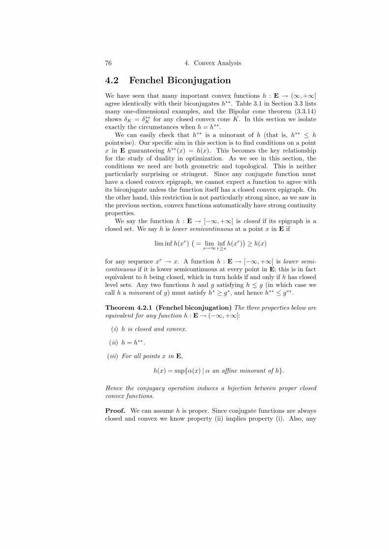
76 4. Convex Analysis
4.2 Fenchel Biconjugation
We have seen that many important convex functions h : E → (∞, +∞]agree identically with their biconjugates h∗∗. Table 3.1 in Section 3.3 listsmany one-dimensional examples, and the Bipolar cone theorem (3.3.14)shows δK = δ∗∗K for any closed convex cone K. In this section we isolateexactly the circumstances when h = h∗∗.
We can easily check that h∗∗ is a minorant of h (that is, h∗∗ ≤ hpointwise). Our specific aim in this section is to find conditions on a pointx in E guaranteeing h∗∗(x) = h(x). This becomes the key relationshipfor the study of duality in optimization. As we see in this section, theconditions we need are both geometric and topological. This is neitherparticularly surprising or stringent. Since any conjugate function musthave a closed convex epigraph, we cannot expect a function to agree withits biconjugate unless the function itself has a closed convex epigraph. Onthe other hand, this restriction is not particularly strong since, as we saw inthe previous section, convex functions automatically have strong continuityproperties.
We say the function h : E → [−∞,+∞] is closed if its epigraph is aclosed set. We say h is lower semicontinuous at a point x in E if
lim inf h(xr)(
= lims→∞
infr≥s
h(xr)) ≥ h(x)
for any sequence xr → x. A function h : E → [−∞,+∞] is lower semi-continuous if it is lower semicontinuous at every point in E; this is in factequivalent to h being closed, which in turn holds if and only if h has closedlevel sets. Any two functions h and g satisfying h ≤ g (in which case wecall h a minorant of g) must satisfy h∗ ≥ g∗, and hence h∗∗ ≤ g∗∗.
Theorem 4.2.1 (Fenchel biconjugation) The three properties below areequivalent for any function h : E → (−∞, +∞]:
(i) h is closed and convex.
(ii) h = h∗∗.
(iii) For all points x in E,
h(x) = supα(x) | α an affine minorant of h.
Hence the conjugacy operation induces a bijection between proper closedconvex functions.
Proof. We can assume h is proper. Since conjugate functions are alwaysclosed and convex we know property (ii) implies property (i). Also, any

4.2 Fenchel Biconjugation 77
affine minorant α of h satisfies α = α∗∗ ≤ h∗∗ ≤ h, and hence property (iii)implies (ii). It remains to show (i) implies (iii).
Fix a point x0 in E. Assume first x0 ∈ cl (dom h), and fix any realr < h(x0). Since h is closed, the set x | h(x) > r is open, so there is anopen convex neighbourhood U of x0 with h(x) > r on U . Now note thatthe set dom h ∩ cont δU is nonempty, so we can apply the Fenchel theorem(3.3.5) to deduce that some element φ of E satisfies
r ≤ infxh(x) + δU (x) = −h∗(φ)− δ∗U (−φ). (4.2.2)
Now define an affine function α(·) = 〈φ, ·〉+ δ∗U (−φ) + r. Inequality (4.2.2)shows that α minorizes h, and by definition we know α(x0) ≥ r. Since rwas arbitrary, (iii) follows at the point x = x0.
Suppose on the other hand x0 does not lie in cl (domh). By the Basicseparation theorem (2.1.6) there is a real b and a nonzero element a of Esatisfying
〈a, x0〉 > b ≥ 〈a, x〉 for all points x in dom h.
The argument in the preceding paragraph shows there is an affine minorantα of h. But now the affine function α(·) + k(〈a, ·〉 − b) is a minorant of hfor all k = 1, 2, . . . . Evaluating these functions at x = x0 proves property(iii) at x0. The final remark follows easily. 2
We immediately deduce that a closed convex function h : E → [−∞, +∞]equals its biconjugate if and only if it is proper or identically +∞ or −∞.
Restricting the conjugacy bijection to finite sublinear functions givesthe following result.
Corollary 4.2.3 (Support functions) Fenchel conjugacy induces a bi-jection between everywhere-finite sublinear functions and nonempty com-pact convex sets in E:
(a) If the set C ⊂ E is compact, convex and nonempty then the supportfunction δ∗C is everywhere finite and sublinear.
(b) If the function h : E → R is sublinear then h∗ = δC , where the set
C = φ ∈ E | 〈φ, d〉 ≤ h(d) for all d ∈ E
is nonempty, compact, and convex.
Proof. See Exercise 9. 2
Conjugacy offers a convenient way to recognize when a convex functionhas bounded level sets.
78 4. Convex Analysis
Theorem 4.2.4 (Moreau–Rockafellar) A closed convex proper func-tion on E has bounded level sets if and only if its conjugate is continuousat 0.
Proof. By Proposition 1.1.5, a convex function f : E → (∞,+∞] hasbounded level sets if and only if it satisfies the growth condition
lim inf‖x‖→∞
f(x)‖x‖ > 0.
Since f is closed we can check that this is equivalent to the existence ofa minorant of the form ε‖ · ‖ + k ≤ f(·) for some constants ε > 0 and k.Taking conjugates, this is in turn equivalent to f∗ being bounded abovenear 0, and the result then follows by Theorem 4.1.1 (Local boundedness).
2
Strict convexity is also easy to recognize via conjugacy, using the fol-lowing result (see Exercise 19 for the proof).
Theorem 4.2.5 (Strict-smooth duality) A proper closed convex func-tion on E is essentially strictly convex if and only if its conjugate is essen-tially smooth.
What can we say about h∗∗ when the function h : E → [−∞,+∞] isnot necessarily closed? To answer this question we introduce the idea ofthe closure of h, denoted cl h, defined by
epi (cl h) = cl (epi h). (4.2.6)
It is easy to verify that cl h is then well-defined. The definition immediatelyimplies clh is the largest closed function minorizing h. Clearly if h isconvex, so is cl h. We leave the proof of the next simple result as anexercise.
Proposition 4.2.7 (Lower semicontinuity and closure) If a functionf : E → [−∞, +∞] is convex then it is lower semicontinuous at a point xwhere it is finite if and only if f(x) = (cl f)(x). In this case f is proper.
We can now answer the question we posed at the beginning of thesection.
Theorem 4.2.8 Suppose the function h : E → [−∞, +∞] is convex.
(a) If h∗∗ is somewhere finite then h∗∗ = cl h.
(b) For any point x where h is finite, h(x) = h∗∗(x) if and only if h islower semicontinuous at x.
4.2 Fenchel Biconjugation 79
Proof. Observe first that since h∗∗ is closed and minorizes h, we knowh∗∗ ≤ clh ≤ h. If h∗∗ is somewhere finite then h∗∗ (and hence cl h) is never−∞ by applying Proposition 4.2.7 (Lower semicontinuity and closure) toh∗∗. On the other hand, if h is finite and lower semicontinuous at x thenProposition 4.2.7 shows cl h(x) is finite, and applying the proposition againto cl h shows once more that cl h is never −∞. In either case, the Fenchelbiconjugation theorem implies cl h = (cl h)∗∗ ≤ h∗∗ ≤ clh, so cl h = h∗∗.Part (a) is now immediate, while part (b) follows by using Proposition 4.2.7once more. 2
Any proper convex function h with an affine minorant has its biconju-gate h∗∗ somewhere finite. (In fact, because E is finite-dimensional, h∗∗ issomewhere finite if and only if h is proper—see Exercise 25.)
Exercises and Commentary
Our approach in this section again extends easily to infinite dimensions;see for example [70]. Our definition of a closed function is a little differentto that in [167], although they coincide for proper functions. The originalversion of von Neumann’s minimax theorem (Exercise 16) had both thesets C and D simplices. The proof was by Brouwer’s fixed point theorem(8.1.3). The Fisher information function introduced in Exercise 24 is usefulin signal reconstruction [35]. The inequality in Exercise 20 (Logarithmichomogeneity) is important for interior point methods [148, Prop. 2.4.1].
1. Prove that any function h : E → [−∞, +∞] satisfies h∗∗ ≤ h.
2. (Lower semicontinuity and closedness) For any given functionh : E → [−∞, +∞], prove the following properties are equivalent:
(a) h is lower semicontinuous.
(b) h has closed level sets.
(c) h is closed.
Prove that such a function has a global minimizer on any nonempty,compact set.
3. (Pointwise maxima) If the functions fγ : E → [−∞, +∞] areall convex (respectively closed) then prove the function defined byf(x) = supγ fγ(x) is convex (respectively closed). Deduce that forany function h : E → [−∞,+∞], the conjugate function h∗ is closedand convex.
4. Verify directly that any affine function equals its biconjugate.
80 4. Convex Analysis
5. ∗ (Midpoint convexity)
(a) A function f : E → (∞, +∞] is midpoint convex if it satisfies
f(x + y
2
)≤ f(x) + f(y)
2for all x and y in E.
Prove a closed function is convex if and only if it is midpointconvex.
(b) Use the inequality
2(X2 + Y 2) º (X + Y )2 for all X and Y in Sn
to prove the function Z ∈ Sn+ 7→ −Z1/2 is Sn
+-convex (see Sec-tion 3.3, Exercise 18 (Order convexity)).
6. Is the Fenchel biconjugation theorem (4.2.1) valid for arbitrary func-tions h : E → [−∞, +∞]?
7. (Inverse of subdifferential) For a function h : E → (∞, +∞], ifpoints x and φ in E satisfy φ ∈ ∂h(x), prove x ∈ ∂h∗(φ). Prove theconverse if h is closed and convex.
8. ∗ (Closed subdifferential) If a function h : E → (∞, +∞] is closed,prove the multifunction ∂h is closed: that is,
φr ∈ ∂h(xr), xr → x, φr → φ ⇒ φ ∈ ∂h(x).
Deduce that if h is essentially smooth and a sequence of points xr inint (dom h) approaches a point in bd (dom h) then ‖∇h(xr)‖ → ∞.
9. ∗ (Support functions)
(a) Prove that if the set C ⊂ E is nonempty then δ∗C is a closedsublinear function and δ∗∗C = δcl convC . Prove that if C is alsobounded then δ∗C is everywhere finite.
(b) Prove that any sets C,D ⊂ E satisfy
δ∗C+D = δ∗C + δ∗D andδ∗conv(C∪D) = max(δ∗C , δ∗D).
(c) Suppose the function h : E → (−∞,+∞] is positively homoge-neous, and define a closed convex set
C = φ ∈ E | 〈φ, d〉 ≤ h(d) ∀d.Prove h∗ = δC . Prove that if h is in fact sublinear and every-where finite then C is nonempty and compact.

4.2 Fenchel Biconjugation 81
(d) Deduce Corollary 4.2.3 (Support functions).
10. ∗ (Almost homogeneous functions [19]) Prove that a functionf : E → R has a representation
f(x) = maxi∈I
〈ai, x〉 − bi (x ∈ E)
for a compact set (ai, bi) | i ∈ I ⊂ E×R if and only if f is convexand satisfies supE |f − g| < ∞ for some sublinear function g.
11. ∗ Complete the details of the proof of the Moreau–Rockafellar theo-rem (4.2.4).
12. (Compact bases for cones) Consider a closed convex cone K.Using the Moreau–Rockafellar theorem (4.2.4), show that a point xlies in intK if and only if the set φ ∈ K− | 〈φ, x〉 ≥ −1 is bounded.If the set φ ∈ K− | 〈φ, x〉 = −1 is nonempty and bounded, provex ∈ intK.
13. For any function h : E → [−∞,+∞], prove the set cl (epi h) is theepigraph of some function.
14. ∗ (Lower semicontinuity and closure) For any convex functionh : E → [−∞, +∞] and any point x0 in E, prove
(clh)(x0) = limδ↓0
inf‖x−x0‖≤δ
h(x).
Deduce Proposition 4.2.7.
15. For any point x in E and any function h : E → (−∞, +∞] with asubgradient at x, prove h is lower semicontinuous at x.
16. ∗ (Von Neumann’s minimax theorem [185]) Suppose Y is aEuclidean space. Suppose that the sets C ⊂ E and D ⊂ Y arenonempty and convex with D closed and that the map A : E → Y islinear.
(a) By considering the Fenchel problem
infx∈E
δC(x) + δ∗D(Ax)
proveinfx∈C
supy∈D
〈y, Ax〉 = maxy∈D
infx∈C
〈y,Ax〉
(where the max is attained if finite), under the assumption
0 ∈ core (dom δ∗D −AC). (4.2.9)

82 4. Convex Analysis
(b) Prove property (4.2.9) holds in either of the two cases
(i) D is bounded, or(ii) A is surjective and 0 lies in intC. (Hint: Use the Open
mapping theorem, Section 4.1, Exercise 9.)
(c) Suppose both C and D are compact. Prove
minx∈C
maxy∈D
〈y,Ax〉 = maxy∈D
minx∈C
〈y, Ax〉.
17. (Recovering primal solutions) Assume all the conditions for theFenchel theorem (3.3.5) hold, and that in addition the functions fand g are closed.
(a) Prove that if the point φ ∈ Y is an optimal dual solution thenthe point x ∈ E is optimal for the primal problem if and only ifit satisfies the two conditions x ∈ ∂f∗(A∗φ) and Ax ∈ ∂g∗(−φ).
(b) Deduce that if f∗ is differentiable at the point A∗φ then the onlypossible primal optimal solution is x = ∇f∗(A∗φ).
(c) ∗∗ Apply this result to the problems in Section 3.3, Exercise 22.
18. Calculate the support function δ∗C of the set C = x ∈ R2 |x2 ≥ x21.
Prove the “contour” y | δ∗C(y) = 1 is not closed.
19. ∗ (Strict-smooth duality) Consider a proper closed convex func-tion f : E → (∞,+∞].
(a) If f has Gateaux derivative y at a point x in E, prove the in-equality
f∗(z) > f∗(y) + 〈x, z − y〉for elements z of E distinct from y.
(b) If f is essentially smooth, prove that f∗ is essentially strictlyconvex.
(c) Deduce the Strict-smooth duality theorem (4.2.5) using Exercise23 in Section 3.1.
20. ∗ (Logarithmic homogeneity) If the function f : E → (∞, +∞]is closed, convex, and proper, then for any real ν > 0 prove theinequality
f(x) + f∗(φ) + ν log 〈x,−φ〉 ≥ ν log ν − ν for all x, φ ∈ E
holds (where we interpret log α = −∞ when α ≤ 0) if and only fsatisfies the condition
f(tx) = f(x)− ν log t for all x ∈ E, t ∈ R++.
4.2 Fenchel Biconjugation 83
Hint: Consider first the case ν = 1, and use the inequality
α ≤ −1− log(−α).
21. ∗ (Cofiniteness) Consider a function h : E → (∞,+∞] and thefollowing properties:
(i) h(·)− 〈φ, ·〉 has bounded level sets for all φ in E.
(ii) lim‖x‖→∞ ‖x‖−1h(x) = +∞.
(iii) h∗ is everywhere finite.
Complete the following steps.
(a) Prove properties (i) and (ii) are equivalent.
(b) If h is closed, convex and proper, use the Moreau–Rockafellartheorem (4.2.4) to prove properties (i) and (iii) are equivalent.
22. ∗∗ (Computing closures)
(a) Prove any closed convex function g : R → (∞, +∞] is continu-ous on its domain.
(b) Consider a convex function f : E → (∞, +∞]. For any points xin E and y in int (dom f), prove
f∗∗(x) = limt↑1
f(y + t(x− y)).
Hint: Use part (a) and the Accessibility lemma (Section 1.1,Exercise 11).
23. ∗∗ (Recession functions) This exercise uses Section 1.1, Exercise 6(Recession cones). The recession function of a closed convex functionf : E → (∞, +∞] is defined by
0+f(d) = supt∈R++
f(x + td)− f(x)t
for d in E,
where x is any point in dom f .
(a) Prove 0+f is closed and sublinear.
(b) Prove epi (0+f) = 0+(epi f), and deduce that 0+f is indepen-dent of the choice of the point x.
(c) For any real α > inf f , prove
0+y ∈ E | f(y) ≤ α = d ∈ E | 0+f(d) ≤ 0.
84 4. Convex Analysis
24. ∗∗ (Fisher information function) Let f : R → (∞,+∞] be agiven function, and define a function g : R2 → (∞,+∞] by
g(x, y) =
yf
(x
y
)if y > 0
+∞ otherwise.
(a) Prove g is convex if and only if f is convex.
(b) Suppose f is essentially strictly convex. For y and v in R++
and x and u in R, prove
g(x, y) + g(u, v) = g(x + y, u + v) ⇔ x
y=
u
v.
(c) Calculate g∗.
(d) Suppose f is closed, convex, and finite at 0. Using Exercises 22and 23, prove
g∗∗(x, y) =
yf(x
y
)if y > 0
0+f(x) if y = 0+∞ otherwise.
(e) If f(x) = x2/2 for all x in R, calculate g.
(f) Define a set C = (x, y) ∈ R2 | x2 ≤ y ≤ x and a function
h(x, y) =
x3
y2if (x, y) ∈ C \ 0
0 if (x, y) = 0+∞ otherwise.
Prove h is closed and convex but is not continuous relative toits (compact) domain C. Construct another such example withsupC h finite.
25. ∗∗ (Finiteness of biconjugate) Consider a convex function h : E →[−∞,+∞].
(a) If h is proper and has an affine minorant, prove h∗∗ is somewherefinite.
(b) If h∗∗ is somewhere finite, prove h is proper.
(c) Use the fact that any proper convex function has a subgradient(Section 3.1, Exercise 29) to deduce that h∗∗ is somewhere finiteif and only if h is proper.
(d) Deduce h∗∗ = cl h for any convex function h : E → (∞, +∞].
4.2 Fenchel Biconjugation 85
26. ∗∗ (Self-dual cones [8]) Consider a function h : E → [−∞,∞) forwhich −h is closed and sublinear, and suppose there is a point x ∈ Esatisfying h(x) > 0. Define the concave polar of h as the functionh : E → [−∞,∞) given by
h(y) = inf〈x, y〉 | h(x) ≥ 1.
(a) Prove −h is closed and sublinear, and, for real λ > 0, we haveλ(λh) = h.
(b) Prove the closed convex cone
Kh = (x, t) ∈ E×R | |t| ≤ h(x)
has polar (Kh)− = −Kh .
(c) Suppose the vector α ∈ Rn++ satisfies
∑i αi = 1, and define a
function hα : Rn → [−∞, +∞) by
hα(x) = ∏
i xαii if x ≥ 0
−∞ otherwise.
Prove hα = hα/hα(α), and deduce the cone
Pα = K(hα(α))−1/2hα
is self-dual: P−α = −Pα.
(d) Prove the cones
Q2 = (x, t, z) ∈ R3 | t2 ≤ 2xz, x, z ≥ 0 and
Q3 = (x, t, z) ∈ R3 | 2|t|3 ≤√
27xz2, x, z ≥ 0
are self-dual.
(e) Prove Q2 is isometric to S2+; in other words, there is a linear map
A : R3 → S2+ preserving the norm and satisfying AQ2 = S2
+.
27. ∗∗ (Conical open mapping [8]) Define two closed convex cones inR3:
Q = (x, y, z) ∈ R3 | y2 ≤ 2xz, x, z ≥ 0. and
S = (w, x, y) ∈ R3 | 2|x|3 ≤√
27wy2, w, y ≥ 0.
These cones are self-dual by Exercise 26. Now define convex cones inR4 by
C = (0×Q) + (S × 0) and D = 0×R3.
(a) Prove C ∩D = 0 ×Q.
86 4. Convex Analysis
(b) Prove −C− = (R×Q) ∩ (S ×R).
(c) Define the projection P : R4 → R3 by P (w, x, y, z) = (x, y, z).Prove P (C−) = −Q, or equivalently,
C− + D− = (C ∩D)−.
(d) Deduce the normal cone formula
NC∩D(x) = NC(x) + ND(x) for all x in C ∩D
and, by taking polars, the tangent cone formula
TC∩D(x) = TC(x) ∩ TD(x) for all x in C ∩D.
(e) Prove C− is a closed convex pointed cone with nonempty interiorand D− is a line, and yet there is no constant ε > 0 satisfying
(C− + D−) ∩ εB ⊂ (C− ∩B) + (D− ∩B).
(Hint: Prove equivalently there is no ε > 0 satisfying
P (C−) ∩ εB ⊂ P (C− ∩B)
by considering the path (t2, t3, t) | t ≥ 0 in Q.) Compare thiswith the situation when C and D are subspaces, using the Openmapping theorem (Section 4.1, Exercise 9).
(f) Consider the path
u(t) =( 2√
27, t2, t3, 0
)if t ≥ 0.
Prove dC(u(t)) = 0 and dD(u(t)) = 2/√
27 for all t ≥ 0, and yet
dC∩D(u(t)) → +∞ as t → +∞.
(Hint: Use the isometry in Exercise 26.)
28. ∗∗ (Expected surprise [18]) An event occurs once every n days,with probability pi on day i for i = 1, 2, . . . , n. We seek a distributionmaximizing the average surprise caused by the event. Define the“surprise” as minus the logarithm of the probability that the eventoccurs on day i given that it has not occurred so far. Using Bayesconditional probability rule, our problem is
inf
S(p)∣∣∣
n∑1
pi = 1
,
4.2 Fenchel Biconjugation 87
where we define the function S : Rn → (∞,+∞] by
S(p) =n∑
i=1
h(pi,
n∑
j=i
pj
),
and the function h : R2 → (∞, +∞] by
h(x, y) =
x log(x
y
)if x, y > 0
0 if x ≥ 0, y = 0+∞ otherwise.
(a) Prove h is closed and convex using Exercise 24 (Fisher informa-tion function).
(b) Hence prove S is closed and convex.
(c) Prove the problem has an optimal solution.
(d) By imitating Section 3.1, Exercise 27 (Maximum entropy), showthe solution p is unique and is expressed recursively by
p1 = µ1, pk = µk
(1−
k−1∑1
pj
)for k = 2, 3, . . . , n,
where the numbers µk are defined by the recursion
µn = 1, µk−1 = µke−µk for k = 2, 3, . . . , n.
(e) Deduce that the components of p form an increasing sequenceand that pn−j is independent of j.
(f) Prove p1 ∼ 1/n for large n.
88 4. Convex Analysis
4.3 Lagrangian Duality
The duality between a convex function h and its Fenchel conjugate h∗
which we outlined earlier is an elegant piece of theory. The real significance,however, lies in its power to describe duality theory for convex programs,one of the most far-reaching ideas in the study of optimization.
We return to the convex program that we studied in Section 3.2:
inff(x) | g(x) ≤ 0, x ∈ E. (4.3.1)
Here the function f and the components g1, g2, . . . , gm : E → (∞, +∞] areconvex, and satisfy ∅ 6= dom f ⊂ ∩m
1 dom gi. As before, the Lagrangianfunction L : E×Rm
+ → (∞, +∞] is defined by L(x; λ) = f(x) + λT g(x).Notice that the Lagrangian encapsulates all the information of the pri-
mal problem (4.3.1): clearly
supλ∈Rm
+
L(x;λ) =
f(x) if x is feasible+∞ otherwise,
so if we denote the optimal value of (4.3.1) by p ∈ [−∞, +∞], we couldrewrite the problem in the following form:
p = infx∈E
supλ∈Rm
+
L(x;λ). (4.3.2)
This makes it rather natural to consider an associated problem
d = supλ∈Rm
+
infx∈E
L(x;λ) (4.3.3)
where d ∈ [−∞, +∞] is called the dual value. Thus the dual problemconsists of maximizing over vectors λ in Rm
+ the dual function Φ(λ) =infx L(x; λ). This dual problem is perfectly well-defined without any as-sumptions on the functions f and g. It is an easy exercise to show the“weak duality inequality” p ≥ d. Notice Φ is concave.
It can happen that the primal value p is strictly larger than the dualvalue d (Exercise 5). In this case we say there is a duality gap. We next in-vestigate conditions ensuring there is no duality gap. As in Section 3.2, thechief tool in our analysis is the primal value function v : Rm → [−∞,+∞],defined by
v(b) = inff(x) | g(x) ≤ b. (4.3.4)
Below we summarize the relationships among these various ideas and piecesof notation.
4.3 Lagrangian Duality 89
Proposition 4.3.5 (Dual optimal value)
(a) The primal optimal value p is v(0).
(b) The conjugate of the value function satisfies
v∗(−λ) =−Φ(λ) if λ ≥ 0
+∞ otherwise.
(c) The dual optimal value d is v∗∗(0).
Proof. Part (a) is just the definition of p. Part (b) follows from theidentities
v∗(−λ) = sup−λT b− v(b) | b ∈ Rm= sup−λT b− f(x) | g(x) + z = b, x ∈ dom f, b ∈ Rm, z ∈ Rm
+= sup−λT (g(x) + z)− f(x) | x ∈ dom f, z ∈ Rm
+= − inff(x) + λT g(x) | x ∈ dom f+ sup−λT z | z ∈ Rm
+
=−Φ(λ) if λ ≥ 0
+∞ otherwise.
Finally, we observe
d = supλ∈Rm
+
Φ(λ) = − infλ∈Rm
+
−Φ(λ) = − infλ∈Rm
+
v∗(−λ) = v∗∗(0),
so part (c) follows. 2
Notice the above result does not use convexity.The reason for our interest in the relationship between a convex function
and its biconjugate should now be clear, in light of parts (a) and (c) above.
Corollary 4.3.6 (Zero duality gap) Suppose the value of the primalproblem (4.3.1) is finite. Then the primal and dual values are equal if andonly if the value function v is lower semicontinuous at 0. In this case theset of optimal dual solutions is −∂v(0).
Proof. By the previous result, there is no duality gap exactly when thevalue function satisfies v(0) = v∗∗(0), so Theorem 4.2.8 proves the firstassertion. By part (b) of the previous result, dual optimal solutions λare characterized by the property 0 ∈ ∂v∗(−λ) or equivalently v∗(−λ) +v∗∗(0) = 0. But we know v(0) = v∗∗(0), so this property is equivalent tothe condition −λ ∈ ∂v(0). 2
This result sheds new light on our proof of the Lagrangian necessaryconditions (3.2.8); the proof in fact demonstrates the existence of a dual
90 4. Convex Analysis
optimal solution. We consider below two distinct approaches to proving theabsence of a duality gap. The first uses the Slater condition, as in Theorem3.2.8, to force attainment in the dual problem. The second (dual) approachuses compactness to force attainment in the primal problem.
Theorem 4.3.7 (Dual attainment) If the Slater condition holds for theprimal problem (4.3.1) then the primal and dual values are equal, and thedual value is attained if finite.
Proof. If p is −∞ there is nothing to prove, since we know p ≥ d. If onthe other hand p is finite then, as in the proof of the Lagrangian necessaryconditions (3.2.8), the Slater condition forces ∂v(0) 6= ∅. Hence v is finiteand lower semicontinuous at 0 (Section 4.2, Exercise 15), and the resultfollows by Corollary 4.3.6 (Zero duality gap). 2
An indirect way of stating the Slater condition is that there is a pointx in E for which the set λ ∈ Rm
+ | L(x; λ) ≥ α is compact for all real α.The second approach uses a “dual” condition to ensure the value functionis closed.
Theorem 4.3.8 (Primal attainment) Suppose that the functions
f, g1, g2, . . . , gm : E → (∞,+∞]
are closed and that for some real λ0 ≥ 0 and some vector λ in Rm+ , the
function λ0f + λT g has compact level sets. Then the value function vdefined by equation (4.3.4) is closed, and the infimum in this equation isattained when finite. Consequently, if the functions f, g1, g2, . . . , gm are,in addition, convex and the dual value for the problem (4.3.1) is not −∞,then the primal and dual values p and d are equal, and the primal value isattained when finite.
Proof. If the points (br, sr) lie in epi v for r = 1, 2, . . . and approachthe point (b, s) then for each integer r there is a point xr in E satisfyingf(xr) ≤ sr + r−1 and g(xr) ≤ br. Hence we deduce
(λ0f + λT g)(xr) ≤ λ0(sr + r−1) + λT br → λ0s + λT b.
By the compact level set assumption, the sequence (xr) has a subsequenceconverging to some point x, and since all the functions are closed, we knowf(x) ≤ s and g(x) ≤ b. We deduce v(b) ≤ s, so (b, s) lies in epi v as werequired. When v(b) is finite, the same argument with (br, sr) replaced by(b, v(b)) for each r shows the infimum is attained.
If the functions f, g1, g2, . . . , gm are convex then we know (from Section3.2) v is convex. If d is +∞ then again from the inequality p ≥ d, there is
4.3 Lagrangian Duality 91
nothing to prove. If d (= v∗∗(0)) is finite then Theorem 4.2.8 shows v∗∗ =cl v, and the above argument shows cl v = v. Hence p = v(0) = v∗∗(0) = d,and the result follows. 2
Notice that if either the objective function f or any one of the constraintfunctions g1, g2, . . . , gm has compact level sets then the compact level setcondition in the above result holds.
Exercises and Commentary
An attractive elementary account of finite-dimensional convex duality the-ory appears in [152]. A good reference for this kind of development ininfinite dimensions is [98]. When the value function v is lower semicontin-uous at 0 we say the problem (4.3.1) is normal; see [167]. If ∂v(0) 6= ∅(or v(0) = −∞) the problem is called stable; see, for example, [6]). For astraightforward account of interior point methods and the penalized linearprogram in Exercise 4 (Examples of duals) see [187, p. 40]. For more onthe minimax theory in Exercise 14 see, for example, [60].
1. (Weak duality) Prove that the primal and dual values p and ddefined by equations (4.3.2) and (4.3.3) satisfy p ≥ d.
2. Calculate the Lagrangian dual of the problem in Section 3.2, Exer-cise 3.
3. (Slater and compactness) Prove the Slater condition holds forproblem (4.3.1) if and only if there is a point x in E for which thelevel sets
λ ∈ Rm+ | − L(x;λ) ≤ α
are compact for all real α.
4. (Examples of duals) Calculate the Lagrangian dual problem for thefollowing problems (for given vectors a1, a2, . . . , am, and c in Rn).
(a) The linear program
infx∈Rn
〈c, x〉 | 〈ai, x〉 ≤ bi for i = 1, 2, . . . ,m.
(b) Another linear program
infx∈Rn
〈c, x〉+ δRn+(x) | 〈ai, x〉 ≤ bi for i = 1, 2, . . . , m.
(c) The quadratic program (for C ∈ Sn++)
infx∈Rn
xT Cx
2
∣∣∣ 〈ai, x〉 ≤ bi for i = 1, 2, . . . ,m
.

92 4. Convex Analysis
(d) The separable problem
infx∈Rn
n∑
j=1
p(xj)∣∣∣ 〈ai, x〉 ≤ bi for i = 1, 2, . . . , m
for a given function p : R → (∞, +∞].
(e) The penalized linear program
infx∈Rn
〈c, x〉+ εlb (x) | 〈ai, x〉 ≤ bi for i = 1, 2, . . . , m
for real ε > 0.
For given matrices A1, A2, . . . , Am, and C in Sn, calculate the dualof the semidefinite program
infX∈Sn
+
tr (CX) + δSn+(X) | tr (AiX) ≤ bi for i = 1, 2, . . . , m,
and the penalized semidefinite program
infX∈Sn
+
tr (CX) + εld X | tr (AiX) ≤ bi for i = 1, 2, . . . ,m
for real ε > 0.
5. (Duffin’s duality gap, continued)
(a) For the problem considered in Section 3.2, Exercise 8, namely
infx∈R2
ex2 | ‖x‖ − x1 ≤ 0 ,
calculate the dual function, and hence find the dual value.
(b) Repeat part (a) with the objective function ex2 replaced by x2.
6. Consider the problem
infexp∗(x1) + exp∗(x2) | x1 + 2x2 − 1 ≤ 0, x ∈ R2.
Write down the Lagrangian dual problem, solve the primal and dualproblems, and verify that the optimal values are equal.
7. Given a matrix C in Sn++, calculate
infX∈Sn
++
tr (CX) | − log(detX) ≤ 0
by Lagrangian duality.
4.3 Lagrangian Duality 93
8. ∗ (Mixed constraints) Explain why an appropriate dual for theproblem
inff(x) | g(x) ≤ 0, h(x) = 0for a function h : dom f → Rk is
supλ∈Rm
+ , µ∈Rk
infx∈dom f
f(x) + λT g(x) + µT h(x).
9. (Fenchel and Lagrangian duality) Let Y be a Euclidean space.By suitably rewriting the primal Fenchel problem
infx∈E
f(x) + g(Ax)
for given functions f : E → (∞, +∞], g : Y → (∞, +∞], and linearA : E → Y, interpret the dual Fenchel problem
supφ∈Y
−f∗(A∗φ)− g∗(−φ)
as a Lagrangian dual problem.
10. (Trust region subproblem duality [175]) Given a matrix A inSn and a vector b in Rn, consider the nonconvex problem
infxT Ax + bT x
∣∣ xT x− 1 ≤ 0, x ∈ Rn.
Complete the following steps to prove there is an optimal dual solu-tion, with no duality gap.
(i) Prove the result when A is positive semidefinite.
(ii) If A is not positive definite, prove the primal optimal value doesnot change if we replace the inequality in the constraint by anequality.
(iii) By observing for any real α the equality
minxT Ax + bT x
∣∣ xT x = 1
=
−α + minxT (A + αI)x + bT x
∣∣ xT x = 1,
prove the general result.
11. ∗∗ If there is no duality gap, prove that dual optimal solutions arethe same as Karush–Kuhn–Tucker vectors (Section 3.2, Exercise 9).
12. ∗ (Conjugates of compositions) Consider the composition g fof a nondecreasing convex function g : R → (∞, +∞] with a convexfunction f : E → (∞,+∞]. We interpret g(+∞) = +∞, and we
94 4. Convex Analysis
assume there is a point x in E satisfying f(x) ∈ int (dom g). UseLagrangian duality to prove the formula, for φ in E,
(g f)∗(φ) = inft∈R+
g∗(t) + tf∗
(φ
t
),
where we interpret
0f∗(φ
0
)= δ∗dom f (φ).
13. ∗∗ (A symmetric pair [28])
(a) Given real γ1, γ2, . . . , γn > 0, define h : Rn → (∞, +∞] by
h(x) = ∏n
i=1 x−γi
i if x ∈ Rn++
+∞ otherwise.
By writing g(x) = exp(log g(x)) and using the composition for-mula in Exercise 12, prove
h∗(y) =
−(γ + 1)
n∏
i=1
(−yi
γi
)γi/(γ+1)
if − y ∈ Rn+
+∞ otherwise,
where γ =∑
i γi.
(b) Given real α1, α2, . . . , αn > 0, define α =∑
i αi and suppose areal µ satisfies µ > α + 1. Now define a function f : Rn ×R →(∞,+∞] by
f(x, s) =
µ−1sµ∏
i x−αii if x ∈ Rn
++, s ∈ R+
+∞ otherwise.
Use part (a) to prove
f∗(y, t) =
ρν−1tν∏
i(−yi)−βi if − y ∈ Rn++, t ∈ R+
+∞ otherwise
for constants
ν =µ
µ− (α + 1), βi =
αi
µ− (α + 1), ρ =
∏
i
(αi
µ
)βi
.
(c) Deduce f = f∗∗, whence f is convex.
(d) Give an alternative proof of the convexity of f by using Section4.2, Exercise 24(a) (Fisher information function) and induction.
(e) Prove f is strictly convex.
4.3 Lagrangian Duality 95
14. ∗∗ (Convex minimax theory) Suppose that Y is a Euclidean space,that the sets C ⊂ Y and D ⊂ E are nonempty, and consider afunction ψ : C ×D → R.
(a) Prove the inequality
supy∈D
infx∈C
ψ(x, y) ≤ infx∈C
supy∈D
ψ(x, y).
(b) We call a point (x, y) in C ×D a saddlepoint if it satisfies
ψ(x, y) ≤ ψ(x, y) ≤ ψ(x, y) for all x ∈ C, y ∈ D.
In this case prove
supy∈D
infx∈C
ψ(x, y) = ψ(x, y) = infx∈C
supy∈D
ψ(x, y).
(c) Suppose the function py : E → (∞, +∞] defined by
py(x) =
ψ(x, y) if x ∈ C+∞ otherwise
is convex, for all y in D. Prove the function h : Y → [−∞, +∞]defined by
h(z) = infx∈C
supy∈D
ψ(x, y) + 〈z, y〉
is convex.
(d) Suppose the function qx : Y → (∞, +∞] defined by
qx(y) =−ψ(x, y) if y ∈ D
+∞ otherwise
is closed and convex for all points x in C. Deduce
h∗∗(0) = supy∈D
infx∈C
ψ(x, y).
(e) Suppose that for all points y in D the function py defined inpart (c) is closed and convex, and that for some point y in D,py has compact level sets. If h is finite at 0, prove it is lowersemicontinuous there. If the assumption in part (d) also holds,deduce
supy∈D
infx∈C
ψ(x, y) = minx∈C
supy∈D
ψ(x, y).
(f) Suppose the functions f, g1, g2, . . . , gs : Rt → (∞, +∞] areclosed and convex. Interpret the above results in the followingtwo cases:

96 4. Convex Analysis
(i) C = (dom f) ∩( s⋂
i=1
dom gi
)
D = Rs+
ψ(u,w) = f(u) +∑s
i=1 wigi(u).
(ii) C = Rs+
D = (dom f) ∩( s⋂
i=1
dom gi
)
ψ(u, w) = −f(w)−∑si=1 uigi(w).
(g) (Kakutani [109]) Suppose that the nonempty sets C ⊂ Y andD ⊂ E are compact and convex, that the function ψ : C ×D →R is continuous, that ψ(x, y) is convex in the variable x for allfixed y in D, and that −ψ(x, y) is convex in the variable y forall points x in C. Deduce ψ has a saddlepoint.
Chapter 5
Special Cases
5.1 Polyhedral Convex Sets and Functions
In our earlier section on theorems of the alternative (Section 2.2), we ob-served that finitely generated cones are closed. Remarkably, a finite linear-algebraic assumption leads to a topological conclusion. In this section wepursue the consequences of this type of assumption in convex analysis.
There are two natural ways to impose a finite linear structure on the setsand functions we consider. The first we have already seen: a “polyhedron”(or polyhedral set) is a finite intersection of closed halfspaces in E, and wesay a function f : E → [−∞, +∞] is polyhedral if its epigraph is polyhedral.On the other hand, a polytope is the convex hull of a finite subset of E,and we call a subset of E finitely generated if it is the sum of a polytopeand a finitely generated cone (in the sense of formula (2.2.11)). Notice wedo not yet know if a cone that is a finitely generated set in this sense isfinitely generated in the sense of (2.2.11); we return to this point later inthe section. The function f is finitely generated if its epigraph is finitelygenerated. A central result of this section is that polyhedra and finitelygenerated sets in fact coincide.
We begin with some easy observations collected together in the followingtwo results.
Proposition 5.1.1 (Polyhedral functions) Suppose that the functionf : E → [−∞, +∞] is polyhedral. Then f is closed and convex and can bedecomposed in the form
f = maxi∈I
gi + δP , (5.1.2)
where the index set I is finite (and possibly empty), the functions gi areaffine, and the set P ⊂ E is polyhedral (and possibly empty). Thus thedomain of f is polyhedral and coincides with dom ∂f if f is proper.
97
98 5. Special Cases
Proof. Since any polyhedron is closed and convex, so is f , and the de-composition (5.1.2) follows directly from the definition. If f is proper thenboth the sets I and P are nonempty in this decomposition. At any pointx in P (= dom f) we know 0 ∈ ∂δP (x), and the function maxi gi certainlyhas a subgradient at x since it is everywhere finite. Hence we deduce thecondition ∂f(x) 6= ∅. 2
Proposition 5.1.3 (Finitely generated functions) Suppose the func-tion f : E → [−∞, +∞] is finitely generated. Then f is closed and convexand dom f is finitely generated. Furthermore, f∗ is polyhedral.
Proof. Polytopes are compact and convex (by Caratheodory’s theorem(Section 2.2, Exercise 5)), and finitely generated cones are closed and con-vex, so finitely generated sets (and therefore functions) are closed and con-vex (by Section 1.1, Exercise 5(a)). We leave the remainder of the proof asan exercise. 2
An easy exercise shows that a set P ⊂ E is polyhedral (respectively, finitelygenerated) if and only if δP is polyhedral (respectively, finitely generated).
To prove that polyhedra and finitely generated sets in fact coincide,we consider the two extreme special cases: first, compact sets, and second,cones. Observe first that compact, finitely generated sets are just polytopes,directly from the definition.
Lemma 5.1.4 Any polyhedron has at most finitely many extreme points.
Proof. Fix a finite set of affine functions gi | i ∈ I on E, and considerthe polyhedron
P = x ∈ E | gi(x) ≤ 0 for i ∈ I.For any point x in P , the “active set” is i ∈ I | gi(x) = 0. Suppose twodistinct extreme points x and y of P have the same active set. Then forany small real ε the points x± ε(y− x) both lie in P . But this contradictsthe assumption that x is extreme. Hence different extreme points havedifferent active sets, and the result follows. 2
This lemma together with Minkowski’s theorem (4.1.8) reveals the na-ture of compact polyhedra.
Theorem 5.1.5 Any compact polyhedron is a polytope.
We next turn to cones.
Lemma 5.1.6 Any polyhedral cone is a finitely generated cone (in thesense of (2.2.11)).
5.1 Polyhedral Convex Sets and Functions 99
Proof. Given a polyhedral cone P ⊂ E, define a subspace L = P ∩ −Pand a pointed polyhedral cone K = P ∩ L⊥. Observe the decompositionP = K ⊕ L. By the Pointed cone theorem (3.3.15), there is an element yof E for which the set
C = x ∈ K | 〈x, y〉 = 1is compact and satisfies K = R+C. Since C is polyhedral, the previousresult shows it is a polytope. Thus K is finitely generated, whence so is P .
2
Theorem 5.1.7 (Polyhedrality) A set or function is polyhedral if andonly if it is finitely generated.
Proof. For finite sets ai | i ∈ I ⊂ E and bi | i ∈ I ⊂ R, consider thepolyhedron in E defined by
P = x ∈ E | 〈ai, x〉 ≤ bi for i ∈ I.The polyhedral cone in E×R defined by
Q = (x, r) ∈ E×R | 〈ai, x〉 − bir ≤ 0 for i ∈ Iis finitely generated by the previous lemma, so there are finite subsetsxj | j ∈ J and yt | t ∈ T of E with
Q = ∑
j∈J
λj(xj , 1)+∑
t∈T
µt(yt, 0)∣∣∣λj ∈ R+ for j ∈ J, µt ∈ R+ for t ∈ T
.
We deduce
P = x | (x, 1) ∈ Q= conv xj | j ∈ J+
∑
t∈T
µtyy
∣∣∣ µt ∈ R+ for t ∈ T
,
so P is finitely generated. We have thus shown that any polyhedral set(and hence function) is finitely generated.
Conversely, suppose the function f : E → [−∞,+∞] is finitely gener-ated. Consider first the case when f is proper. By Proposition 5.1.3, f∗
is polyhedral, and hence (by the above argument) finitely generated. Butf is closed and convex, by Proposition 5.1.3, so the Fenchel biconjugationtheorem (4.2.1) implies f = f∗∗. By applying Proposition 5.1.3 once againwe see f∗∗ (and hence f) is polyhedral. We leave the improper case as anexercise. 2
Notice these two results show our two notions of a finitely generated conedo indeed coincide.
The following collection of exercises shows that many linear-algebraicoperations preserve polyhedrality.
100 5. Special Cases
Proposition 5.1.8 (Polyhedral algebra) Consider a Euclidean spaceY and a linear map A : E → Y.
(a) If the set P ⊂ E is polyhedral then so is its image AP .
(b) If the set K ⊂ Y is polyhedral then so is its inverse image A−1K.
(c) The sum and pointwise maximum of finitely many polyhedral func-tions are polyhedral.
(d) If the function g : Y → [−∞,+∞] is polyhedral then so is the com-posite function g A.
(e) If the function q : E × Y → [−∞, +∞] is polyhedral then so is thefunction h : Y → [−∞, +∞] defined by h(u) = infx∈E q(x, u).
Corollary 5.1.9 (Polyhedral Fenchel duality) All the conclusions ofthe Fenchel duality theorem (3.3.5) remain valid if the regularity condi-tion (3.3.8) is replaced by the assumption that the functions f and g arepolyhedral with dom g ∩Adom f nonempty.
Proof. We follow the original proof, simply observing that the value func-tion h defined in the proof is polyhedral by the Polyhedral algebra propo-sition above. Thus, when the optimal value is finite, h has a subgradientat 0. 2
We conclude this section with a result emphasizing the power of Fenchelduality for convex problems with linear constraints.
Corollary 5.1.10 (Mixed Fenchel duality) All the conclusions of theFenchel duality theorem (3.3.5) remain valid if the regularity condition(3.3.8) is replaced by the assumption that dom g ∩ Acont f is nonemptyand the function g is polyhedral.
Proof. Assume without loss of generality the primal optimal value
p = infx∈E
f(x) + g(Ax) = infx∈E, r∈R
f(x) + r | g(Ax) ≤ r
is finite. By assumption there is a feasible point for the problem on theright at which the objective function is continuous, so there is an affinefunction α : E × R → R minorizing the function (x, r) 7→ f(x) + r suchthat
p = infx∈E, r∈R
α(x, r) | g(Ax) ≤ r
(see Section 3.3, Exercise 13(c)). Clearly α has the form α(x, r) = β(x)+ rfor some affine minorant β of f , so
p = infx∈E
β(x) + g(Ax).
5.1 Polyhedral Convex Sets and Functions 101
Now we apply polyhedral Fenchel duality (Corollary 5.1.9) to deduce theexistence of an element φ of Y such that
p = −β∗(A∗φ)− g∗(−φ) ≤ −f∗(A∗φ)− g∗(−φ) ≤ p
(using the weak duality inequality), and the duality result follows. Thecalculus rules follow as before. 2
It is interesting to compare this result with the version of Fenchel dual-ity using the Open mapping theorem (Section 4.1, Exercise 9), where theassumption that g is polyhedral is replaced by surjectivity of A.
Exercises and Commentary
Our approach in this section is analogous to [181]. The key idea, Theorem5.1.7 (Polyhedrality), is due to Minkowski [141] and Weyl [186]. A nicedevelopment of geometric programming (see Exercise 13) appears in [152].
1. Prove directly from the definition that any polyhedral function has adecomposition of the form (5.1.2).
2. Fill in the details for the proof of the Finitely generated functionsproposition (5.1.3).
3. Use Proposition 4.2.7 (Lower semicontinuity and closure) to showthat if a finitely generated function f is not proper then it has theform
f(x) =
+∞ if x 6∈ K−∞ if x ∈ K
for some finitely generated set K.
4. Prove a set K ⊂ E is polyhedral (respectively, finitely generated) ifand only if δK is polyhedral (respectively, finitely generated). Do notuse the Polyhedrality theorem (5.1.7).
5. Complete the proof of the Polyhedrality theorem (5.1.7) for improperfunctions using Exercise 3.
6. (Tangents to polyhedra) Prove the tangent cone to a polyhedronP at a point x in P is given by TP (x) = R+(P − x).
7. ∗ (Polyhedral algebra) Prove Proposition 5.1.8 using the followingsteps.
(i) Prove parts (a)–(d).
102 5. Special Cases
(ii) In the notation of part (e), consider the natural projection
PY×R : E×Y ×R → Y ×R.
Prove the inclusions
PY×R(epi q) ⊂ epi h ⊂ cl (PY×R(epi q)).
(iii) Deduce part (e).
8. If the function f : E → (∞, +∞] is polyhedral, prove the subdiffer-ential of f at a point x in dom f is a nonempty polyhedron and isbounded if and only if x lies in int (dom f).
9. (Polyhedral cones) For any polyhedral cones H ⊂ Y and K ⊂ Eand any linear map A : E → Y, prove the relation
(K ∩A−1H)− = A∗H− + K−
using convex calculus.
10. Apply the Mixed Fenchel duality corollary (5.1.10) to the probleminff(x) | Ax ≤ b, for a linear map A : E → Rm and a point b inRm.
11. ∗ (Generalized Fenchel duality) Consider convex functions
h1, h2, . . . , hm : E → (∞,+∞]
with ∩iconthi nonempty. By applying the Mixed Fenchel dualitycorollary (5.1.10) to the problem
infx,x1,x2,...,xm∈E
m∑
i=1
hi(xi)∣∣∣ xi = x for i = 1, 2, . . . ,m
,
prove
infx∈E
∑
i
hi(x) = − inf ∑
i
h∗i (φi)
∣∣∣ φ1, φ2, . . . , φm ∈ E,∑
i
φi = 0
.
12. ∗∗ (Relativizing Mixed Fenchel duality) In the Mixed Fenchelduality corollary (5.1.10), prove the condition dom g ∩ Acont f 6= ∅can be replaced by dom g ∩Ari (dom f) 6= ∅.
13. ∗∗ (Geometric programming) Consider the constrained geometricprogram
infx∈E
h0(x) | hi(x) ≤ 1 for i = 1, 2, . . . , m,

5.1 Polyhedral Convex Sets and Functions 103
where each function hi is a sum of functions of the form
x ∈ E 7→ c log( n∑
j=1
exp 〈aj , x〉)
for real c > 0 and elements a1, a2, . . . , an of E. Write down theLagrangian dual problem and simplify it using Exercise 11 and theform of the conjugate of each hi given by (3.3.1). State a dualitytheorem.

104 5. Special Cases
5.2 Functions of Eigenvalues
Fenchel conjugacy gives a concise and beautiful avenue to many eigenvalueinequalities in classical matrix analysis. In this section we outline thisapproach.
The two cones Rn+ and Sn
+ appear repeatedly in applications, as do theircorresponding logarithmic barriers lb and ld , which we defined in Section3.3. We can relate the vector and matrix examples, using the notation ofSection 1.2, through the identities
δSn+
= δRn+ λ and ld = lb λ. (5.2.1)
We see in this section that these identities fall into a broader pattern.Recall the function [·] : Rn → Rn rearranges components into nonin-
creasing order. We say a function f on Rn is symmetric if f(x) = f([x])for all vectors x in Rn; in other words, permuting components does notchange the function value. We call a symmetric function of the eigenvaluesof a symmetric matrix a spectral function. The following formula is crucial.
Theorem 5.2.2 (Spectral conjugacy) If f : Rn → [−∞,+∞] is a sym-metric function, it satisfies the formula
(f λ)∗ = f∗ λ.
Proof. By Fan’s inequality (1.2.2) any matrix Y in Sn satisfies the in-equalities
(f λ)∗(Y ) = supX∈Sn
tr (XY )− f(λ(X))
≤ supXλ(X)T λ(Y )− f(λ(X))
≤ supx∈Rn
xT λ(Y )− f(x)
= f∗(λ(Y )).
On the other hand, fixing a spectral decomposition Y = UT (Diag λ(Y ))Ufor some matrix U in On leads to the reverse inequality
f∗(λ(Y )) = supx∈Rn
xT λ(Y )− f(x)
= supxtr ((Diag x)UY UT )− f(x)
= supxtr (UT (Diag x)UY )− f(λ(UT DiagxU))
≤ supX∈Sn
tr (XY )− f(λ(X))
= (f λ)∗(Y ),

5.2 Functions of Eigenvalues 105
which completes the proof. 2
This formula, for example, makes it very easy to calculate ld ∗ (see the Logbarriers proposition (3.3.3)) and to check the self-duality of the cone Sn
+.Once we can compute conjugates easily, we can also recognize closed
convex functions easily using the Fenchel biconjugation theorem (4.2.1).
Corollary 5.2.3 (Davis) Suppose the function f : Rn → (∞, +∞] issymmetric. Then the “spectral function” f λ is closed and convex if andonly if f is closed and convex.
We deduce immediately that the logarithmic barrier ld is closed and con-vex, as well as the function X 7→ tr (X−1) on Sn
++, for example.Identifying subgradients is also easy using the conjugacy formula and
the Fenchel–Young inequality (3.3.4).
Corollary 5.2.4 (Spectral subgradients) If f : Rn → (∞, +∞] is asymmetric function, then for any two matrices X and Y in Sn, the follow-ing properties are equivalent:
(i) Y ∈ ∂(f λ)(X).
(ii) X and Y have a simultaneous ordered spectral decomposition andsatisfy λ(Y ) ∈ ∂f(λ(X)).
(iii) X = UT (Diag x)U and Y = UT (Diag y)U for some matrix U in On
and vectors x and y in Rn satisfying y ∈ ∂f(x).
Proof. Notice the inequalities
(f λ)(X) + (f λ)∗(Y ) = f(λ(X)) + f∗(λ(Y )) ≥ λ(X)T λ(Y ) ≥ tr (XY ).
The condition Y ∈ ∂(fλ)(X) is equivalent to equality between the left andright hand sides (and hence throughout), and the equivalence of properties(i) and (ii) follows using Fan’s inequality (1.2.1). For the remainder of theproof, see Exercise 9. 2
Corollary 5.2.5 (Spectral differentiability) Suppose that the functionf : Rn → (∞,+∞] is symmetric, closed, and convex. Then f λ isdifferentiable at a matrix X in Sn if and only if f is differentiable at λ(X).
Proof. If ∂(f λ)(X) is a singleton, so is ∂f(λ(X)), by the Spectralsubgradients corollary above. Conversely, suppose ∂f(λ(X)) consists onlyof the vector y ∈ Rn. Using Exercise 9(b), we see the components of yare nonincreasing, so by the same corollary, ∂(f λ)(X) is the nonemptyconvex set
UT (Diag y)U | U ∈ On, UT Diag (λ(X))U = X.

106 5. Special Cases
But every element of this set has the same norm (namely ‖y‖), so the setmust be a singleton. 2
Notice that the proof in fact shows that when f is differentiable at λ(X)we have the formula
∇(f λ)(X) = UT (Diag∇f(λ(X)))U (5.2.6)
for any matrix U in On satisfying UT (Diagλ(X))U = X.The pattern of these results is clear: many analytic and geometric prop-
erties of the matrix function f λ parallel the corresponding properties ofthe underlying function f . The following exercise is another example.
Corollary 5.2.7 Suppose the function f : Rn → (∞, +∞] is symmetric,closed, and convex. Then fλ is essentially strictly convex (respectively, es-sentially smooth) if and only if f is essentially strictly convex (respectively,essentially smooth).
For example, the logarithmic barrier ld is both essentially smooth andessentially strictly convex.
Exercises and Commentary
Our approach in this section follows [120]. The Davis theorem (5.2.3) ap-peared in [58] (without the closure assumption). Many convexity propertiesof eigenvalues like Exercise 4 (Examples of convex spectral functions) canbe found in [99] or [10], for example. Surveys of eigenvalue optimizationappear in [128, 127].
1. Prove the identities (5.2.1).
2. Use the Spectral conjugacy theorem (5.2.2) to calculate ld ∗ and δ∗Sn+.
3. Prove the Davis characterization (Corollary 5.2.3) using the Fenchelbiconjugation theorem (4.2.1).
4. (Examples of convex spectral functions) Use the Davis char-acterization (Corollary 5.2.3) to prove the following functions of amatrix X ∈ Sn are closed and convex:
(a) ld (X).
(b) tr (Xp), for any nonnegative even integer p.
(c)−tr (X1/2) if X ∈ Sn
+
+∞ otherwise.

5.2 Functions of Eigenvalues 107
(d)
tr (X−p) if X ∈ Sn++
+∞ otherwisefor any nonnegative integer p.
(e)
tr (X1/2)−1 if X ∈ Sn++
+∞ otherwise.
(f)−(detX)1/n if X ∈ Sn
+
+∞ otherwise.
Deduce from the sublinearity of the function in part (f) the property
0 ¹ X ¹ Y ⇒ 0 ≤ det X ≤ detY
for matrices X and Y in Sn.
5. Calculate the conjugate of each of the functions in Exercise 4.
6. Use formula (5.2.6) to calculate the gradients of the functions in Ex-ercise 4.
7. For a matrix A in Sn++ and a real b > 0, use the Lagrangian sufficient
conditions (3.2.3) to solve the problem
inff(X) | tr (AX) ≤ b, X ∈ Sn,
where f is one of the functions in Exercise 4.
8. ∗ (Orthogonal invariance) A function h : Sn → (∞,+∞] is or-thogonally invariant if all matrices X in Sn and U in On satisfy therelation h(UT XU) = h(X); in other words, orthogonal similaritytransformations do not change the value of h.
(a) Prove h is orthogonally invariant if and only if there is a sym-metric function f : Rn → (∞, +∞] with h = f λ.
(b) Prove that an orthogonally invariant function h is closed andconvex if and only if h Diag is closed and convex.
9. ∗ Suppose the function f : Rn → (−∞, +∞] is symmetric.
(a) Prove f∗ is symmetric.
(b) If vectors x and y in Rn satisfy y ∈ ∂f(x), prove [y] ∈ ∂f([x])using Proposition 1.2.4.
(c) Finish the proof of the Spectral subgradients corollary (5.2.4).
(d) Deduce ∂(f λ)(X) = ∅ ⇔ ∂f(λ(X)) = ∅.(e) Prove Corollary 5.2.7.
108 5. Special Cases
10. ∗ (Fillmore–Williams [78]) Suppose the set C ⊂ Rn is symmetric:that is, PC = C holds for all permutation matrices P . Prove the set
λ−1(C) = X ∈ Sn | λ(X) ∈ C
is closed and convex if and only if C is closed and convex.
11. ∗∗ (Semidefinite complementarity) Suppose matrices X and Ylie in Sn
+.
(a) If tr (XY ) = 0, prove −Y ∈ ∂δSn+(X).
(b) Hence prove the following properties are equivalent:
(i) tr (XY ) = 0.(ii) XY = 0.(iii) XY + Y X = 0.
(c) Using Exercise 5 in Section 1.2, prove for any matrices U and Vin Sn
(U2 + V 2)1/2 = U + V ⇔ U, V º 0 and tr (UV ) = 0.
12. ∗∗ (Eigenvalue sums) Consider a vector µ in Rn≥.
(a) Prove the function µT λ(·) is sublinear using Section 2.2, Exercise9 (Schur-convexity).
(b) Deduce the map λ is (−Rn≥)−-sublinear. (See Section 3.3, Ex-
ercise 18 (Order convexity).)
(c) Use Section 3.1, Exercise 10 to prove
∂(µT λ)(0) = λ−1(conv (Pnµ)).
13. ∗∗ (Davis theorem) Suppose the function f : Rn → [−∞, +∞] issymmetric (but not necessarily closed). Use Exercise 12 (Eigenvaluesums) and Section 2.2, Exercise 9(d) (Schur-convexity) to prove thatf λ is convex if and only if f is convex.
14. ∗ (DC functions) We call a real function f on a convex set C ⊂ Ea DC function if it can be written as the difference of two real convexfunctions on C.
(a) Prove the set of DC functions is a vector space.
(b) If f is a DC function, prove it is locally Lipschitz on intC.
(c) Prove λk is a DC function on Sn for all k, and deduce it is locallyLipschitz.

5.3 Duality for Linear and Semidefinite Programming 109
5.3 Duality for Linear and SemidefiniteProgramming
Linear programming (LP) is the study of optimization problems involv-ing a linear objective function subject to linear constraints. This simpleoptimization model has proved enormously powerful in both theory andpractice, so we devote this section to deriving linear programming dualitytheory from our convex-analytic perspective. We contrast this theory withthe corresponding results for semidefinite programming (SDP), a class ofmatrix optimization problems analogous to linear programs but involvingthe positive semidefinite cone.
Linear programs are inherently polyhedral, so our main developmentfollows directly from the polyhedrality section (Section 5.1). But to be-gin, we sketch an alternative development directly from the Farkas lemma(2.2.7). Given vectors a1, a2, . . . , am, and c in Rn and a vector b in Rm,consider the primal linear program
inf 〈c, x〉subject to 〈ai, x〉 − bi ≤ 0 for i = 1, 2, . . . , m
x ∈ Rn.
(5.3.1)
Denote the primal optimal value by p ∈ [−∞, +∞]. In the Lagrangianduality framework (Section 4.3), the dual problem is
sup− bT µ
∣∣∣m∑
i=1
µiai = −c, µ ∈ Rm
+
(5.3.2)
with dual optimal value d ∈ [−∞, +∞]. From Section 4.3 we know theweak duality inequality p ≥ d. If the primal problem (5.3.1) satisfies theSlater condition then the Dual attainment theorem (4.3.7) shows p = dwith dual attainment when the values are finite. However, as we shall see,the Slater condition is superfluous here.
Suppose the primal value p is finite. Then it is easy to see that the“homogenized” system of inequalities in Rn+1,
〈ai, x〉 − biz ≤ 0 for i = 1, 2, . . . ,m−z ≤ 0 and
〈−c, x〉+ pz > 0, x ∈ Rn, z ∈ R
(5.3.3)
has no solution. Applying the Farkas lemma (2.2.7) to this system, wededuce there is a vector µ in Rn
+ and a scalar β in R+ satisfying
m∑
i=1
µi(ai,−bi) + β(0,−1) = (−c, p).

110 5. Special Cases
Thus µ is a feasible solution for the dual problem (5.3.2) with objectivevalue at least p. The weak duality inequality now implies µ is optimal andp = d. We needed no Slater condition; the assumption of a finite primaloptimal value alone implies zero duality gap and dual attainment.
We can be more systematic using our polyhedral theory. Suppose thatY is a Euclidean space, that the map A : E → Y is linear, and considercones H ⊂ Y and K ⊂ E. For given elements c of E and b of Y, considerthe primal abstract linear program
inf〈c, x〉 |Ax− b ∈ H, x ∈ K. (5.3.4)
As usual, denote the optimal value by p. We can write this problem inFenchel form (3.3.6) if we define functions f on E and g on Y by f(x) =〈c, x〉+δK(x) and g(y) = δH(y−b). Then the Fenchel dual problem (3.3.7)is
sup〈b, φ〉 |A∗φ− c ∈ K−, φ ∈ −H− (5.3.5)
with dual optimal value d. If we now apply the Fenchel duality theorem(3.3.5) in turn to problem (5.3.4), and then to problem (5.3.5) (using theBipolar cone theorem (3.3.14)), we obtain the following general result.
Corollary 5.3.6 (Cone programming duality) Suppose the cones Hand K in problem (5.3.4) are convex.
(a) If any of the conditions
(i) b ∈ int (AK −H),
(ii) b ∈ AK − intH, or
(iii) b ∈ A(intK)−H, and either H is polyhedral or A is surjective
hold then there is no duality gap (p = d) and the dual optimal valued is attained if finite.
(b) Suppose H and K are also closed. If any of the conditions
(i) −c ∈ int (A∗H− + K−),
(ii) −c ∈ A∗H− + intK−, or
(iii) −c ∈ A∗(int H−) + K−, and either K is polyhedral or A∗ issurjective
hold then there is no duality gap and the primal optimal value p isattained if finite.
In both parts (a) and (b), the sufficiency of condition (iii) follows by ap-plying the Mixed Fenchel duality corollary (5.1.10), or the Open mappingtheorem (Section 4.1, Exercise 9). In the fully polyhedral case we obtainthe following result.
5.3 Duality for Linear and Semidefinite Programming 111
Corollary 5.3.7 (Linear programming duality) Suppose the cones Hand K in the dual pair of problems (5.3.4) and (5.3.5) are polyhedral. Ifeither problem has finite optimal value then there is no duality gap and bothproblems have optimal solutions.
Proof. We apply the Polyhedral Fenchel duality corollary (5.1.9) to eachproblem in turn. 2
Our earlier result for the linear program (5.3.1) is clearly just a special caseof this corollary.
Linear programming has an interesting matrix analogue. Given matri-ces A1, A2, . . . , Am, and C in Sn
+ and a vector b in Rm, consider the primalsemidefinite program
inf tr (CX)subject to tr (AiX) = bi for i = 1, 2, . . . , m
X ∈ Sn+.
(5.3.8)
This is a special case of the abstract linear program (5.3.4), so the dualproblem is
sup
bT φ∣∣∣ C −
m∑
i=1
φiAi ∈ Sn+, φ ∈ Rm
, (5.3.9)
since (Sn+)− = −Sn
+, by the Self-dual cones proposition (3.3.12), and weobtain the following duality theorem from the general result above.
Corollary 5.3.10 (Semidefinite programming duality) If the primalproblem (5.3.8) has a positive definite feasible solution, there is no dualitygap and the dual optimal value is attained when finite. On the other hand,if there is a vector φ in Rm with C −∑
i φiAi positive definite then onceagain there is no duality gap and the primal optimal value is attained whenfinite.
Unlike linear programming, we need a condition stronger than mereconsistency to guarantee no duality gap. For example, if we consider theprimal semidefinite program (5.3.8) with
n = 2, m = 1, C =[
0 11 0
], A1 =
[1 00 0
], and b = 0,
the primal optimal value is 0 (and is attained), whereas the dual problem(5.3.9) is inconsistent.

112 5. Special Cases
Exercises and Commentary
The importance of linear programming duality was first emphasized byDantzig [57] and that of semidefinite duality by Nesterov and Nemirovskii[148]. A good general reference for linear programming is [53]. A straight-forward exposition of the central path (see Exercise 10) may be found in[187]. Semidefinite programming has wide application in control theory[46].
1. Check the form of the dual problem for the linear program (5.3.1).
2. If the optimal value of problem (5.3.1) is finite, prove system (5.3.3)has no solution.
3. (Linear programming duality gap) Give an example of a linearprogram of the form (5.3.1) which is inconsistent (p = +∞) with thedual problem (5.3.2) also inconsistent (d = −∞).
4. Check the form of the dual problem for the abstract linear program(5.3.4).
5. Fill in the details of the proof of the Cone programming duality corol-lary (5.3.6). In particular, when the cones H and K are closed, showhow to interpret problem (5.3.4) as the dual of problem (5.3.5).
6. Fill in the details of the proof of the linear programming dualitycorollary (5.3.7).
7. (Complementary slackness) Suppose we know the optimal valuesof problems (5.3.4) and (5.3.5) are equal and the dual value is at-tained. Prove a feasible solution x for problem (5.3.4) is optimal ifand only if there is a feasible solution φ for the dual problem (5.3.5)satisfying the conditions
〈Ax− b, φ〉 = 0 = 〈x,A∗φ− c〉.
8. (Semidefinite programming duality) Prove Corollary 5.3.10.
9. (Semidefinite programming duality gap) Check the details ofthe example after Corollary 5.3.10.
10. ∗∗ (Central path) Consider the dual pair of linear programs (5.3.1)and (5.3.2). Define a linear map A : Rn → Rm by (Ax)i = (ai)T xfor each index i. Make the following assumptions:
(i) There is a vector x in Rn satisfying b−Ax ∈ Rn++.
(ii) There is a feasible solution µ in Rm++ for problem (5.3.2).

5.3 Duality for Linear and Semidefinite Programming 113
(iii) The set a1, a2, . . . , am is linearly independent.
Now consider the “penalized” problem (for real ε > 0)
infx∈Rn
cT x + εlb (b−Ax). (5.3.11)
(a) Write this problem as a Fenchel problem (3.3.6), and show thedual problem is
sup− bT µ− εlb (µ)−k(ε)
∣∣∣m∑
i=1
µiai = −c, µ ∈ Rm
+
(5.3.12)
for some function k : R+ → R.
(b) Prove that both problems (5.3.11) and (5.3.12) have optimalsolutions, with equal optimal values.
(c) By complementary slackness (Section 3.3, Exercise 9(f)), proveproblems (5.3.11) and (5.3.12) have unique optimal solutionsxε ∈ Rn and µε ∈ Rm, characterized as the unique solution ofthe system
m∑
i=1
µiai = −c
µi(bi − (ai)T x) = ε for each i
b−Ax ≥ 0, andµ ∈ Rm
+ , x ∈ Rn.
(d) Calculate cT xε + bT µε.
(e) Deduce that, as ε decreases to 0, the feasible solution xε ap-proaches optimality in problem (5.3.1) and µε approaches opti-mality in problem (5.3.2).
11. ∗∗ (Semidefinite central path) Imitate the development of Exer-cise 10 for the semidefinite programs (5.3.8) and (5.3.9).
12. ∗∗ (Relativizing cone programming duality) Prove other condi-tions guaranteeing part (a) of Corollary 5.3.6 are
(i) b ∈ A(riK)− riH or
(ii) b ∈ A(riK)−H and H polyhedral.
(Hint: Use Section 4.1, Exercise 20, and Section 5.1, Exercise 12.)
114 5. Special Cases
5.4 Convex Process Duality
In this section we introduce the idea of a “closed convex process”. Theseare set-valued maps whose graphs are closed convex cones. As such, theyprovide a powerful unifying formulation for the study of linear maps, convexcones, and linear programming. The exercises show the elegance of thisapproach in a range of applications.
Throughout this section we fix a Euclidean space Y. For clarity, wedenote the closed unit balls in E and Y by BE and BY, respectively. Amultifunction (or set-valued map) Φ : E → Y is a map from E to the setof subsets of Y. The domain of Φ is the set
D(Φ) = x ∈ E | Φ(x) 6= ∅.
We say Φ has nonempty images if its domain is E. For any subset C ofE we write Φ(C) for the image ∪x∈CΦ(x), and the range of Φ is the setR(Φ) = Φ(E). We say Φ is surjective if its range is Y. The graph of Φ isthe set
G(Φ) = (x, y) ∈ E×Y | y ∈ Φ(x),and we define the inverse multifunction Φ−1 : Y → E by the relationship
x ∈ Φ−1(y) ⇔ y ∈ Φ(x) for x in E and y in Y.
A multifunction is convex, or closed, or polyhedral if its graph is likewise.A process is a multifunction whose graph is a cone. For example, we caninterpret linear maps as closed convex processes in the obvious way.
Closure is one example of a variety of continuity properties of multi-functions we study in this section. We say the multifunction Φ is LSC ata point (x0, y) in its graph if, for all neighbourhoods V of y, the imageΦ(x) intersects V for all points x close to x0. (In particular, x0 must lie inint (D(Φ)).) Equivalently, for any sequence of points (xn) approaching x0
there is a sequence of points yn ∈ Φ(xn) approaching y. If, for x0 in thedomain, this property holds for all points y in Φ(x0), we say Φ is LSC atx0. (The notation comes from “lower semicontinuous”, a name we avoidin this context because of incompatibility with the single-valued case; seeExercise 5.)
On the other hand, we say Φ is open at a point (x, y0) in its graph if, forall neighbourhoods U of x, the point y0 lies in int (Φ(U)). (In particular,y0 must lie in int (R(Φ)).) Equivalently, for any sequence of points (yn)approaching y0 there is a sequence of points (xn) approaching x such thatyn ∈ Φ(xn) for all n. If, for y0 in the range, this property holds for allpoints x in Φ−1(y0), we say Φ is open at y0. These properties are inverseto each other in the following sense.

5.4 Convex Process Duality 115
Proposition 5.4.1 (Openness and lower semicontinuity) Any multi-function Φ : E → Y is LSC at a point (x, y) in its graph if and only if Φ−1
is open at (y, x).
We leave the proof as an exercise.For convex multifunctions, openness at a point in the graph has strong
global implications: the following result is another exercise.
Proposition 5.4.2 If a convex multifunction is open at some point in itsgraph then it is open throughout the interior of its range.
In particular, a convex process Φ : E → Y is open at (0, 0) ∈ E×Y ifand only if it is open at 0 ∈ Y; we just say Φ is open at zero (or, dually,Φ−1 is LSC at zero).
There is a natural duality for convex processes that generalizes theadjoint operation for linear maps. For a convex process Φ : E → Y, wedefine the adjoint process Φ∗ : Y → E by
G(Φ∗) = (µ, ν) | (ν,−µ) ∈ G(Φ)−.
Then an easy consequence of the Bipolar cone theorem (3.3.14) is
G(Φ∗∗) = −G(Φ),
providing Φ is closed. (We could define a “lower” adjoint by the relationshipΦ∗(µ) = −Φ∗(−µ), in which case (Φ∗)∗ = Φ.)
The language of adjoint processes is elegant and concise for many vari-ational problems involving cones. A good example is the cone program(5.3.4). We can write this problem as
infx∈E
〈c, x〉 | b ∈ Ψ(x),
where Ψ is the closed convex process defined by
Ψ(x) =
Ax−H if x ∈ K∅ otherwise (5.4.3)
for points c in E, b in Y, and closed convex cones H ⊂ Y and K ⊂ E. Aneasy calculation shows the adjoint process is
Ψ∗(µ) =
A∗µ + K− if µ ∈ H−
∅ otherwise, (5.4.4)
so we can write the dual problem (5.3.5) as
supµ∈Y
〈b, µ〉 | − c ∈ Ψ∗(−µ). (5.4.5)
116 5. Special Cases
Furthermore, the constraint qualifications in the Cone programming dualitycorollary (5.3.6) become simply b ∈ intR(Ψ) and −c ∈ intR(Ψ∗).
In Section 1.1 we mentioned the fundamental linear-algebraic fact thatthe null space of any linear map A and the range of its adjoint satisfy therelationship
(A−1(0))− = R(A∗). (5.4.6)
Our next step is to generalize this to processes. We begin with an easylemma.
Lemma 5.4.7 Any convex process Φ : E → Y and subset C of Y satisfyΦ∗(C) ⊂ (Φ−1(C)).
Equality in this relationship requires more structure.
Theorem 5.4.8 (Adjoint process duality) Let Φ : E → Y be a convexprocess, and suppose the set C ⊂ Y is convex with R(Φ) ∩ C nonempty.
(a) Either of the assumptions
(i) the multifunction x ∈ E 7→ Φ(x) − C is open at zero (or, inparticular, intC contains zero), or
(ii) Φ and C are polyhedral
implies(Φ−1(C)) = Φ∗(C).
(b) On the other hand, if C is compact and Φ is closed then
(Φ−1(C)) = cl (Φ∗(C)).
Proof. Suppose assumption (i) holds in part (a). For a fixed element φof (Φ−1(C)), we can check that the “value function” v : Y → [−∞, +∞]defined for elements y of Y by
v(y) = infx∈E
−〈φ, x〉 | y ∈ Φ(x)− C (5.4.9)
is convex. The assumption φ ∈ (Φ−1(C)) is equivalent to v(0) ≥ −1,while the openness assumption implies 0 ∈ core (dom v). Thus v is properby Lemma 3.2.6, and so the Max formula (3.1.8) shows v has a subgradient−λ ∈ Y at 0. A simple calculation now shows λ ∈ C and φ ∈ Φ∗(λ),which, together with Lemma 5.4.7, proves the result.
If Φ and C are polyhedral, the Polyhedral algebra proposition (5.1.8)shows v is also polyhedral, so again has a subgradient, and our argumentproceeds as before.

5.4 Convex Process Duality 117
Turning to part (b), we can rewrite φ ∈ (Φ−1(C)) as
(φ, 0) ∈ (G(Φ) ∩ (E× C))
and apply the polarity formula in Section 4.1, Exercise 8 to deduce
(φ, 0) ∈ cl (G(Φ)− + (0× C)).
Hence there are sequences (φn,−ρn) in G(Φ)− and µn in C with φn ap-proaching φ and µn − ρn approaching 0. We deduce
φn ∈ Φ∗(ρn) ⊂ Φ∗(C + εnBY),
where the real sequence εn = ‖µn − ρn‖ approaches 0. Since C is boundedwe know int (C) contains 0 (by Section 4.1, Exercise 5), and the resultfollows using the positive homogeneity of Φ∗. 2
The null space/range formula (5.4.6) thus generalizes to a closed convexprocess Φ:
(Φ−1(0)) = cl (R(Φ∗)),
and the closure is not required if Φ is open at zero.We are mainly interested in using these polarity formulae to relate two
“norms” for a convex process Φ : E → Y. The “lower norm”
‖Φ‖l = infr ∈ R++ | Φ(x) ∩ rBY 6= ∅, ∀x ∈ BEquantifies Φ being LSC at zero; it is easy to check that Φ is LSC at zero ifand only if its lower norm is finite. The “upper norm”
‖Φ‖u = infr ∈ R++ | Φ(BE) ⊂ rBYquantifies a form of “upper semicontinuity” (see Section 8.2). Clearly Φis bounded (that is, bounded sets have bounded images) if and only if itsupper norm is finite. Both norms generalize the norm of a linear mapA : E → Y, defined by
‖A‖ = sup‖Ax‖ | ‖x‖ ≤ 1.Theorem 5.4.10 (Norm duality) Any closed convex process Φ satisfies
‖Φ‖l = ‖Φ∗‖u.
Proof. For any real r > ‖Φ‖l we know BE ⊂ Φ−1(rBY) by definition.Taking polars implies BE ⊃ r−1Φ∗(BY), by the Adjoint process dualitytheorem (5.4.8), whence ‖Φ∗‖u < r.
Conversely, ‖Φ∗‖u < r implies Φ∗(BY) ⊂ rBE. Taking polars andapplying the Adjoint process duality theorem again followed by the Bipolar
118 5. Special Cases
set theorem (4.1.5) shows BE ⊂ r(cl (Φ−1(BY))). But since BY is compactwe can check Φ−1(BY) is closed, and the result follows. 2
The values of the upper and lower norms of course depend on the spacesE and Y. Our proof of the Norm duality theorem above shows that itremains valid when BE and BY denote unit balls for arbitrary norms (seeSection 4.1, Exercise 2), providing we replace them by their polars B
E andB
Y in the definition of ‖Φ∗‖u.The next result is an immediate consequence of the Norm duality the-
orem.
Corollary 5.4.11 A closed convex process is LSC at zero if and only if itsadjoint is bounded.
We are now ready to prove the main result of this section.
Theorem 5.4.12 (Open mapping) The following properties of a closedconvex process Φ are equivalent:
(i) Φ is open at zero.
(ii) (Φ∗)−1 is bounded.
(iii) Φ is surjective.
Proof. The equivalence of parts (i) and (ii) is just Corollary 5.4.11 (aftertaking inverses and observing the identity G((Φ∗)−1) = −G((Φ−1)∗). Part(i) clearly implies part (iii), so it remains to prove the converse. But if Φis surjective then we know
Y =∞⋃
n=1
Φ(nBE) =∞⋃
n=1
nΦ(BE),
so zero lies in the core, and hence the interior, of the convex set Φ(BE).Thus Φ is open at zero. 2
Taking inverses gives the following equivalent result.
Theorem 5.4.13 (Closed graph) The following properties of a closedconvex process Φ are equivalent:
(i) Φ is LSC at zero.
(ii) Φ∗ is bounded.
(iii) Φ has nonempty images.
5.4 Convex Process Duality 119
Exercises and Commentary
A classic reference for multifunctions is [13], and [113] is a good com-pendium which includes applications in mathematical economics. Convexprocesses were introduced by Rockafellar [166, 167]. The power of normedconvex processes was highlighted by Robinson [161, 162]. Our developmenthere follows [23, 24]. The importance of the “distance to inconsistency”(Exercise 21) was first made clear in [160]. For broad extensions, see [66].
1. (Inverse multifunctions) For any multifunction Φ : E → Y, prove
(a) R(Φ−1) = D(Φ).
(b) G(Φ−1) = (y, x) ∈ Y ×E | (x, y) ∈ G(Φ).2. (Convex images) Prove the image of a convex set under a convex
multifunction is convex.
3. For any proper closed convex function f : E → (∞, +∞], prove∂(f∗) = (∂f)−1.
4. Prove Proposition 5.4.1 (Openness and lower semicontinuity).
5. (LSC and lower semicontinuity) For a function f : E → [−∞,∞],suppose f is finite at a point z ∈ E.
(a) Prove f is continuous at z if and only if the multifunction
t ∈ R 7→ f−1(t)
is open at (f(z), z).
(b) Prove f is lower semicontinuous at z if and only if the multi-function whose graph is epi (−f) is LSC at (z, f(z)).
6. ∗ Prove Proposition 5.4.2. (Hint: See Section 4.1, Exercise 1(b).)
7. (Biconjugation) Prove any closed convex process Φ satisfies
G(Φ∗∗) = −G(Φ).
8. Check the adjoint formula (5.4.4).
9. Prove Lemma 5.4.7.
10. Prove the value function (5.4.9) is convex.
11. ∗ Write a complete proof of the Adjoint process duality theorem(5.4.8).
120 5. Special Cases
12. If the multifunction Φ : E → Y is closed and the set C ⊂ Y iscompact, prove Φ−1(C) is closed.
13. Prove G((Φ∗)−1) = −G((Φ−1)∗) for any closed convex process Φ.
14. (Linear maps) Consider a linear map A : E → Y, and define amultifunction Φ : E → Y by Φ(x) = Ax for all points x in E.
(a) Prove Φ is a closed convex process.
(b) Prove Φ∗ is the closed convex process y ∈ Y 7→ A∗y.(c) Prove ‖Φ‖l = ‖Φ‖u = ‖A‖.(d) Prove A is an open map (that is, A maps open sets to open sets)
if and only if Φ is open throughout Y.
(e) Hence deduce the Open mapping theorem for linear maps (Sec-tion 4.1, Exercise 9) as a special case of Theorem 5.4.12.
(f) For any closed convex process Ω : E → Y, prove
(Ω + A)∗ = Ω∗ + A∗.
15. ∗ (Normal cones) A closed convex cone K ⊂ E is generating if itsatisfies K −K = E. For a point x in E, the order interval [0, x]K isthe set K ∩ (x−K). We say K is normal if there is a real c > 0 suchthat
y ∈ [0, x]K ⇒ ‖y‖ ≤ c‖x‖.(a) Prove the multifunction Φ : E → E defined by Φ(x) = [0, x]K is
a closed convex process.
(b) Calculate (Φ∗)−1.
(c) (Krein–Grossberg) Deduce K is normal if and only if K− isgenerating.
(d) Use Section 3.3, Exercise 20 (Pointed cones) to deduce K isnormal if and only if it is pointed.
16. (Inverse boundedness) By considering the convex process (5.4.3),demonstrate the following equivalence for any linear map A : E → Yand closed cones K ⊂ E and H ⊂ Y:
AK −H = Y ⇔ y ∈ H− |A∗y ∈ BE −K− is bounded.
17. ∗∗ (Localization [24]) Given a closed convex process Φ : E → Y anda point b in Y, define the “homogenized” process Ψ : E×R → Y×Rby
Ψ(x, t) =
(Φ(x)− tb)× (t−R+) if t ≥ 0∅ if t < 0.

5.4 Convex Process Duality 121
(a) Prove Ψ is a closed convex process.(b) Prove Ψ is surjective if and only if b lies in core (R(Φ)).(c) Prove Ψ is open at zero if and only if Φ is open at b.(d) Calculate Ψ∗.(e) Prove the following statements are equivalent:
(i) Φ is open at b.(ii) b lies in core (R(Φ)).(iii) The set
µ ∈ Y | Φ∗(µ) ∩BE 6= ∅ and 〈µ, b〉 ≤ 1is bounded.
(f) If R(Φ) has nonempty core, use a separation argument to provethe statements in part (e) are equivalent to
µ ∈ (Φ∗)−1(0) | 〈µ, b〉 ≤ 0 = 0.18. ∗∗ (Cone duality) By applying part (e) of Exercise 17 to example
(5.4.3) with A = 0 and K = E, deduce that a point b lies in the coreof the closed convex cone H ⊂ Y if and only if the set
µ ∈ H− | − 〈µ, b〉 ≤ 1is bounded. Hence, give another proof that a closed convex cone hasa bounded base if and only if its polar has nonempty interior (Section3.3, Exercise 20).
19. ∗∗ (Order epigraphs)
(a) Suppose C ⊂ E is a convex cone, S ⊂ Y is a closed convex cone,and F : C → Y is an S-sublinear function (Section 3.3, Exercise18 (Order convexity)). Prove the multifunction Φ : E → Ydefined by
Φ(x) =
F (x) + S if x ∈ C∅ otherwise,
is a convex process, with adjoint
Φ∗(µ) =
∂〈µ, F (·)〉(0) if µ ∈ −S−
∅ otherwise.
(b) Use Section 5.2, Exercise 12 to prove the adjoint of the closedconvex process
X ∈ Sn 7→ λ(X)− (Rn≥
)−
is the closed convex process with domain Rn≥ defined by
µ 7→ λ−1(conv (Pnµ)).

122 5. Special Cases
20. ∗∗ (Condition number [123]) Consider any closed convex processΦ : E → Y and a linear map G : E → Y.
(a) If ‖G‖−1 > ‖Φ−1‖u, prove the process (Φ + G)−1 is bounded.
(b) If ‖G‖−1 > ‖Φ−1‖l, use part (a) to prove the process Φ + G issurjective.
(c) Suppose Φ is surjective and the point y lies on the boundary ofthe set Φ(BE). By considering a supporting hyperplane, provethere is a rank-one linear map G : E → Y defined by
Gx = 〈µ, x〉yfor some element µ of E such that Φ + G is not surjective.
(d) Deduce
min‖G‖ | Φ + G not surjective = ‖Φ−1‖−1l ,
where the minimum is attained by a rank-one map when finite.
21. ∗∗ (Distance to inconsistency [123]) Consider a given linear mapA : E → Y and an element b of Y. Suppose the space E×R has thenorm ‖(x, t)‖ = ‖x‖+ |t|.(a) Prove the linear map
(x, t) ∈ E×R 7→ Ax− tb
has norm ‖A‖ ∨ ‖b‖.Now consider closed convex cones P ⊂ E and Q ⊂ Y, and systems
(S) b−Ax ∈ Q, x ∈ P and(Sz) z + tb−Ax ∈ Q, x ∈ P, t ∈ R+, ‖x‖+ |t| ≤ 1.
Let I denote the set of pairs (A, b) such that system (S) is inconsis-tent, and let I0 denote the set of (A, b) such that the process
(x, t) ∈ E×R 7→
Ax− tb + Q if x ∈ P, t ∈ R+
∅ if otherwise
is not surjective.
(b) Prove I = cl I0.
(c) By applying Exercise 20 (Condition number), prove the distanceof (A, b) from I is given by the formula
dI(A, b) = inf‖z‖ | (Sz) inconsistent.

Chapter 6
Nonsmooth Optimization
6.1 Generalized Derivatives
From the perspective of optimization, the subdifferential ∂f(·) of a con-vex function f has many of the useful properties of the derivative. Someexamples: it gives the necessary optimality condition 0 ∈ ∂f(x) when thepoint x is a (local) minimizer (Proposition 3.1.5); it reduces to ∇f(x)when f is differentiable at x (Corollary 3.1.10); and it often satisfies certaincalculus rules such as ∂(f + g)(x) = ∂f(x) + ∂g(x) (Theorem 3.3.5). For avariety of reasons, if the function f is not convex, the subdifferential ∂f(·)is not a particularly helpful idea. This makes it very tempting to look fordefinitions of the subdifferential for a nonconvex function. In this sectionwe outline some examples; the most appropriate choice often depends oncontext.
For a convex function f : E → (∞,+∞] with x in dom f , we cancharacterize the subdifferential via the directional derivative: φ ∈ ∂f(x)if and only if 〈φ, ·〉 ≤ f ′(x; ·) (Proposition 3.1.6). A natural approach istherefore to generalize the directional derivative. Henceforth in this sectionwe make the simplifying assumption that the real function f (a real-valuedfunction defined on some subset of E) is locally Lipschitz around the pointx in E.
Partly motivated by the development of optimality conditions, a simplefirst try is the Dini directional derivative:
f−(x;h) = lim inft↓0
f(x + th)− f(x)t
.
A disadvantage of this idea is that f−(x; ·) is not usually sublinear (considerfor example f = −| · | on R), so we could not expect an analogue of theMax formula (3.1.9). With this in mind, we introduce the Clarke directional
123
124 6. Nonsmooth Optimization
derivative,
f(x;h) = lim supy→x, t↓0
f(y + th)− f(y)t
= infδ>0
sup‖y−x‖≤δ, 0<t<δ
f(y + th)− f(y)t
and the Michel–Penot directional derivative,
f¦(x;h) = supu∈E
lim supt↓0
f(x + th + tu)− f(x + tu)t
.
Proposition 6.1.1 If the real function f has Lipschitz constant K aroundthe point x in E then the Clarke and Michel–Penot directional derivativesf(x; ·) and f¦(x; ·) are sublinear and satisfy
f−(x; ·) ≤ f¦(x; ·) ≤ f(x; ·) ≤ K‖ · ‖.
Proof. The positive homogeneity and upper bound are straightforward,so let us prove subadditivity in the Clarke case. For any sequences xr → xin E and tr ↓ 0 in R, and any real ε > 0, we have
f(xr + tr(u + v))− f(xr + tru)tr
≤ f(x; v) + ε
andf(xr + tru)− f(xr)
tr≤ f(x; u) + ε
for all large r. Adding and letting r approach ∞ shows
f(x;u + v) ≤ f(x;u) + f(x; v) + 2ε,
and the result follows. We leave the Michel–Penot case as an exercise. Theinequalities are straightforward. 2
Using our knowledge of support functions (Corollary 4.2.3), we can nowdefine the Clarke subdifferential
∂f(x) = φ ∈ E | 〈φ, h〉 ≤ f(x;h) for all h ∈ E
and the Dini and Michel–Penot subdifferentials ∂−f(x) and ∂¦f(x) analo-gously. Elements of the respective subdifferentials are called subgradients.We leave the proof of the following result as an exercise.
Corollary 6.1.2 (Nonsmooth max formulae) If the real function fhas Lipschitz constant K around the point x in E then the Clarke and

6.1 Generalized Derivatives 125
Michel–Penot subdifferentials ∂f(x) and ∂¦f(x) are nonempty, compact,and convex, and satisfy
∂−f(x) ⊂ ∂¦f(x) ⊂ ∂f(x) ⊂ KB.
Furthermore, the Clarke and Michel–Penot directional derivatives are thesupport functions of the corresponding subdifferentials:
f(x; h) = max〈φ, h〉 | φ ∈ ∂f(x) (6.1.3)
andf¦(x; h) = max〈φ, h〉 | φ ∈ ∂¦f(x) (6.1.4)
for any direction h in E.
Notice the Dini subdifferential is also compact and convex, but may beempty.
Clearly if the point x is a local minimizer of f then any direction h inE satisfies f−(x;h) ≥ 0, and hence the necessary optimality conditions
0 ∈ ∂−f(x) ⊂ ∂¦f(x) ⊂ ∂f(x)
hold. If g is another real function which is locally Lipschitz around x thenwe would not typically expect ∂(f + g)(x) = ∂f(x) + ∂g(x) (considerf = −g = | · | on R at x = 0, for example). On the other hand, if weare interested in an optimality condition like 0 ∈ ∂(f + g)(x), it is thesum rule ∂(f + g)(x) ⊂ ∂f(x) + ∂g(x) that really matters. (A goodexample we see later is Corollary 6.3.9.) We address this in the next result,along with an analogue of the formula for the convex subdifferential of amax-function in Section 3.3, Exercise 17. We write f ∨ g for the functionx 7→ maxf(x), g(x).Theorem 6.1.5 (Nonsmooth calculus) If the real functions f and gare locally Lipschitz around the point x in E, then the Clarke subdifferentialsatisfies
∂(f + g)(x) ⊂ ∂f(x) + ∂g(x) (6.1.6)
and∂(f ∨ g)(x) ⊂ conv (∂f(x) ∪ ∂g(x)). (6.1.7)
Analogous results hold for the Michel–Penot subdifferential.
Proof. The Clarke directional derivative satisfies
(f + g)(x; ·) ≤ f(x; ·) + g(x; ·),since lim sup is a sublinear function. Using the Max formula (6.1.3) wededuce
δ∗∂(f+g)(x) ≤ δ∗∂f(x)+∂g(x)
126 6. Nonsmooth Optimization
and taking conjugates now gives the result using the Fenchel biconjugationtheorem (4.2.1) and the fact that both sides of inclusion (6.1.6) are compactand convex.
To see inclusion (6.1.7), fix a direction h in E and choose sequencesxr → x in E and tr ↓ 0 in R satisfying
(f ∨ g)(xr + trh)− (f ∨ g)(xr)tr
→ (f ∨ g)(x; h).
Without loss of generality, suppose (f ∨ g)(xr + trh) = f(xr + trh) for allr in some subsequence R of N, and now note
f(x;h) ≥ lim supr→∞, r∈R
f(xr + trh)− f(xr)tr
≥ lim supr→∞, r∈R
(f ∨ g)(xr + trh)− (f ∨ g)(xr)tr
= (f ∨ g)(x; h).
We deduce (f ∨ g)(x; ·) ≤ f(x; ·)∨ g(x; ·), which, using the Max formula(6.1.3), we can rewrite as
δ∗∂(f∨g)(x) ≤ δ∗∂f(x) ∨ δ∗∂g(x) = δ∗conv(∂f(x)∪∂g(x))
using Exercise 9(b) (Support functions) in Section 4.2. Now the Fenchelbiconjugation theorem again completes the proof. The Michel–Penot caseis analogous. 2
We now have the tools to derive a nonsmooth necessary optimalitycondition.
Theorem 6.1.8 (Nonsmooth necessary condition) Suppose the pointx is a local minimizer for the problem
inff(x) | gi(x) ≤ 0 (i ∈ I), (6.1.9)
where the real functions f and gi (for i in finite index set I) are locallyLipschitz around x. Let I(x) = i | gi(x) = 0 be the active set. Then thereexist real λ0, λi ≥ 0 for i in I(x), not all zero, satisfying
0 ∈ λ0∂¦f(x) +∑
i∈I(x)
λi∂¦gi(x). (6.1.10)
If, furthermore, some direction d in E satisfies
g¦i (x; d) < 0 for all i in I(x) (6.1.11)
then we can assume λ0 = 1.

6.1 Generalized Derivatives 127
Proof. Imitating the approach of Section 2.3, we note that x is a localminimizer of the function
x 7→ maxf(x)− f(x), gi(x) for i ∈ I(x).
We deduce
0 ∈ ∂¦(maxf − f(x), gi for i ∈ I(x))(x)
⊂ conv(∂¦f(x) ∪
⋃
i∈I(x)
∂¦gi(x))
by inclusion (6.1.7).If condition (6.1.11) holds and λ0 is zero in condition (6.1.10), we obtain
the contradiction
0 ≤ max〈φ, d〉
∣∣∣ φ ∈∑
i∈I(x)
λi∂¦gi(x)
=∑
i∈I(x)
λig¦i (x; d) < 0.
Thus λ0 is strictly positive, and hence without loss of generality equals one.2
Condition (6.1.10) is a Fritz John type condition analogous to Theorem2.3.6. Assumption (6.1.11) is a Mangasarian–Fromovitz type constraintqualification like Assumption 2.3.7, and the conclusion is a Karush–Kuhn–Tucker condition analogous to Theorem 2.3.8. We used the Michel–Penotsubdifferential in the above argument because it is in general smaller thanthe Clarke subdifferential, and hence provides stronger necessary condi-tions. By contrast to our approach here, the developments in Section 2.3and Section 3.2 do not assume the local Lipschitz condition around theoptimal point x.
Exercises and Commentary
Dini derivatives were first used in [64]. The Clarke subdifferential appearedin [54]. A good reference is [55]. The Michel–Penot subdifferential wasintroduced in [138, 139]. A good general reference for this material is [5].
1. (Examples of nonsmooth derivatives) For the following func-tions f : R → R defined for each point x in R by
(a) f(x) = |x|,(b) f(x) = −|x|,
(c) f(x) =
x2 sin(x−1) if x 6= 00 if x = 0,
128 6. Nonsmooth Optimization
(d) f(x) =
3n if 3n ≤ x ≤ 2(3n) for any integer n2x− 3n+1 if 2(3n) ≤ x ≤ 3n+1 for any integer n0 if x ≤ 0,
compute the Dini, Michel–Penot and Clarke directional derivativesand subdifferentials at x = 0.
2. (Continuity of Dini derivative) For a point x in E, prove thefunction f−(x; ·) is Lipschitz if f is locally Lipschitz around x.
3. Complete the proof of Proposition 6.1.1.
4. (Surjective Dini subdifferential) Suppose the continuous functionf : E → R satisfies the growth condition
lim‖x‖→∞
f(x)‖x‖ = +∞.
For any element φ of E, prove there is a point x in E with φ in∂−f(x).
5. Prove Corollary 6.1.2 (Nonsmooth max formulae) using Corollary4.2.3 (Support functions).
6. (Failure of Dini calculus) Show that the inclusion
∂−(f + g)(x) ⊂ ∂−f(x) + ∂−g(x)
can fail for locally Lipschitz functions f and g.
7. ∗ Complete the details of the proof of the Nonsmooth calculus theo-rem (6.1.5).
8. ∗ Prove the following results:
(a) f(x;−h) = (−f)(x;h).
(b) (λf)(x; h) = λf(x; h) for 0 ≤ λ ∈ R.
(c) ∂(λf)(x) = λ∂f(x) for all λ in R.
Derive similar results for the Michel–Penot version.
9. ∗ (Mean value theorem [119])
(a) Suppose the function f : E → R is locally Lipschitz. For anypoints x and y in E, prove there is a real t in (0,1) satisfying
f(x)− f(y) ∈ 〈x− y, ∂¦f(tx + (1− t)y)〉.(Hint: Consider a local minimizer or maximizer of the functiong : [0, 1] → R defined by g(t) = f(tx + (1− t)y).)

6.1 Generalized Derivatives 129
(b) (Monotonicity and convexity) If the set C in E is open andconvex and the function f : C → R is locally Lipschitz, prove fis convex if and only if it satisfies
〈x− y, φ−ψ〉 ≥ 0 for all x, y ∈ C, φ ∈ ∂¦f(x), and ψ ∈ ∂¦f(y).
(c) If ∂¦f(y) ⊂ kB for all points y near x, prove f has local Lipschitzconstant k about x.
Prove similar results for the Clarke case.
10. ∗ (Max-functions) Consider a compact set T ⊂ Rn and a continu-ous function g : E×T → R. For each element t of T define a functiongt : E → R by gt(x) = g(x, t) and suppose, for all t, that this functionis locally Lipschitz around the point z. Define G : E → R by
G(x) = maxg(x, t) | t ∈ T
and let Tz be the set t ∈ T | g(z, t) = G(z). Prove the inclusion
∂G(z) ⊂ cl(conv
⋃
t∈Tz
lim φr | zr → z, tr → t, φr ∈ ∂gtr (zr)
).
Specialize to the case where T is finite, and to the case where ∇gt(x)is a continuous function of (x, t).
11. ∗∗ (Order statistics [125]) Calculate the Dini, the Michel–Penot,and the Clarke directional derivatives and subdifferentials of the func-tion
x ∈ Rn 7→ [x]k.

130 6. Nonsmooth Optimization
6.2 Regularity and Strict Differentiability
We have outlined in Section 2.3 and Section 3.2 two very distinct versionsof the necessary optimality conditions in constrained optimization. Thefirst, culminating in the Karush–Kuhn–Tucker conditions (2.3.8), relied onGateaux differentiability, while the second, leading to the Lagrangian nec-essary conditions (3.2.8), used convexity. A primary aim of the nonsmooththeory of this chapter is to unify these types of results; in this section weshow how this is possible.
A principal feature of the Michel–Penot subdifferential is that it coin-cides with the Gateaux derivative when this exists.
Proposition 6.2.1 (Unique Michel–Penot subgradient) A real func-tion f which is locally Lipschitz around the point x in E has a uniqueMichel–Penot subgradient φ at x if and only if φ is the Gateaux derivative∇f(x).
Proof. If f has a unique Michel–Penot subgradient φ at x, then all direc-tions h in E satisfy
f¦(x; h) = supu∈E
lim supt↓0
f(x + th + tu)− f(x + tu)t
= 〈φ, h〉.
The cases h = w with u = 0 and h = −w with u = w show
lim supt↓0
f(x + tw)− f(x)t
≤ 〈φ,w〉 ≤ lim inft↓0
f(x + tw)− f(x)t
,
so we deduce f ′(x,w) = 〈φ, w〉 as required.Conversely, if f has Gateaux derivative φ at x then any directions h
and u in E satisfy
lim supt↓0
f(x + th + tu)− f(x + tu)t
≤ lim supt↓0
f(x + t(h + u))− f(x)t
− lim inft↓0
f(x + tu)− f(x)t
= f ′(x;h + u)− f ′(x; u)= 〈φ, h + u〉 − 〈φ, u〉 = 〈φ, h〉 = f ′(x; h) ≤ f¦(x;h).
Now taking the supremum over u shows f¦(x;h) = 〈φ, h〉 for all h, as weclaimed. 2
Thus, for example, the Fritz John condition (6.1.10) reduces to Theorem2.3.6 in the differentiable case (under the extra, locally Lipschitz assump-tion).
6.2 Regularity and Strict Differentiability 131
The above result shows that when f is Gateaux differentiable at thepoint x, the Dini and Michel–Penot directional derivatives coincide. Ifthey also equal the Clarke directional derivative then we say f is regularat x. Thus a real function f , locally Lipschitz around x, is regular at xexactly when the ordinary directional derivative f ′(x; ·) exists and equalsthe Clarke directional derivative f(x; ·).
One of the reasons we are interested in regularity is that when the twofunctions f and g are regular at x, the nonsmooth calculus rules (6.1.6)and (6.1.7) hold with equality (assuming f(x) = g(x) in the latter). Theproof is a straightforward exercise.
We know that a convex function is locally Lipschitz around any pointin the interior of its domain (Theorem 4.1.3). In fact such functions arealso regular at such points: consequently our various subdifferentials areall generalizations of the convex subdifferential.
Theorem 6.2.2 (Regularity of convex functions) Suppose the func-tion f : E → (∞,+∞] is convex. If the point x lies in int (dom f) thenf is regular at x, and hence the convex, Dini, Michel–Penot and Clarkesubdifferentials all coincide:
∂f(x) = ∂¦f(x) = ∂−f(x) = ∂f(x).
Proof. Fix a direction h in E and choose a real δ > 0. Denoting the localLipschitz constant by K, we know
f(x; h) = limε↓0
sup‖y−x‖≤εδ
sup0<t<ε
f(y + th)− f(y)t
= limε↓0
sup‖y−x‖≤εδ
f(y + εh)− f(y)ε
≤ limε↓0
f(x + εh)− f(x)ε
+ 2Kδ
= f ′(x; h) + 2Kδ,
using the convexity of f . We deduce
f(x; h) ≤ f ′(x; h) = f−(x; h) ≤ f¦(x; h) ≤ f(x;h),
and the result follows. 2
Thus, for example, the Karush–Kuhn–Tucker type condition that we ob-tained at the end of Section 6.1 reduces exactly to the Lagrangian necessaryconditions (3.2.8), written in the form 0 ∈ ∂f(x) +
∑i∈I(x) λi∂gi(x), as-
suming the convex functions f and gi (for indices i in I(x)) are continuousat the optimal solution x.
132 6. Nonsmooth Optimization
By analogy with Proposition 6.2.1 (Unique Michel–Penot subgradient),we might ask when the Clarke subdifferential of a function f at a point xis a singleton φ? Clearly in this case f must be regular with Gateauxderivative ∇f(x) = φ, although Gateaux differentiability is not enough, asthe example x2 sin(1/x) shows (Exercise 1 in Section 6.1). To answer thequestion we need a stronger notion of differentiability.
For future reference we introduce three gradually stronger conditionsfor an arbitrary real function f . We say an element φ of E is the Frechetderivative of f at x if it satisfies
limy→x, y 6=x
f(y)− f(x)− 〈φ, y − x〉‖y − x‖ = 0,
and we say φ is the strict derivative of f at x if it satisfies
limy,z→x, y 6=z
f(y)− f(z)− 〈φ, y − z〉‖y − z‖ = 0.
In either case, it is easy to see ∇f(x) is φ. For locally Lipschitz functions onE, a straightforward exercise shows Gateaux and Frechet differentiabilitycoincide, but notice that the function x2 sin(1/x) is not strictly differen-tiable at zero. Finally, if f is Gateaux differentiable close to x with gradientmap ∇f(·) continuous then we say f is continuously differentiable aroundx. In the case E = Rn we see in elementary calculus that this is equivalentto the partial derivatives of f being continuous around x. We make analo-gous definitions of Gateaux, Frechet, strict and continuous differentiabilityfor a function F : E → Y (where Y is another Euclidean space). Thederivative ∇f(x) is in this case a linear map from E to Y.
The following result clarifies the idea of a strict derivative and suggestsits connection with the Clarke directional derivative; we leave the proof asanother exercise.
Theorem 6.2.3 (Strict differentiability) A real function f has strictderivative φ at a point x in E if and only if it is locally Lipschitz around xwith
limy→x, t↓0
f(y + th)− f(y)t
= 〈φ, h〉
for all directions h in E. In particular this holds if f is continuously dif-ferentiable around x with ∇f(x) = φ.
We can now answer our question about the Clarke subdifferential.
Theorem 6.2.4 (Unique Clarke subgradient) A real function f whichis locally Lipschitz around the point x in E has a unique Clarke subgradientφ at x if and only if φ is the strict derivative of f at x. In this case f isregular at x.
6.2 Regularity and Strict Differentiability 133
Proof. One direction is clear, so let us assume ∂f(x) = φ. Then wededuce
lim infy→x, t↓0
f(y + th)− f(y)t
= − lim supy→x, t↓0
f((y + th)− th)− f(y + th)t
= −f(x;−h) = 〈φ, h〉 = f(x; h)
= lim supy→x, t↓0
f(y + th)− f(y)t
,
and the result now follows using Theorem 6.2.3 (Strict differentiability).2
The Clarke subdifferential has a remarkable alternative description, of-ten more convenient for computation. It is a reasonably straightforwardmeasure-theoretic consequence of Rademacher’s theorem (9.1.2), whichstates that locally Lipschitz functions are almost everywhere differentiable.
Theorem 6.2.5 (Intrinsic Clarke subdifferential) Suppose that thereal function f is locally Lipschitz around the point x in E and that the setS ⊂ E has measure zero. Then the Clarke subdifferential of f at x is
∂f(x) = conv limr∇f(xr) | xr → x, xr 6∈ S.
Exercises and Commentary
Again, references for this material are [55, 138, 139, 5]. A nice proof ofTheorem 6.2.5 (Intrinsic Clarke subdifferential) appears in [14]. For somerelated ideas applied to distance functions, see [33]. Rademacher’s theoremcan be found in [71], for example. See also Section 9.1. For more detailson the functions of eigenvalues appearing in Exercise 15, see [121, 124].
1. Which of the functions in Section 6.1, Exercise 1 are regular at zero?
2. (Regularity and nonsmooth calculus) If the functions f and gare regular at the point x, prove that the nonsmooth calculus rules(6.1.6) and (6.1.7) hold with equality (assuming f(x) = g(x) in thelatter) and that the resulting functions are also regular at x.
3. Show by a direct calculation that the function x ∈ R 7→ x2 sin(1/x)is not strictly differentiable at the point x = 0.
4. Prove the special case of the Lagrangian necessary conditions weclaim after Theorem 6.2.2.
5. ∗ Prove that the notions of Gateaux and Frechet differentiability co-incide for locally Lipschitz real functions.
134 6. Nonsmooth Optimization
6. Without using Theorem 6.2.4, prove that a unique Clarke subgradientimplies regularity.
7. ∗ Prove the Strict differentiability theorem (6.2.3).
8. Write out a complete proof of the unique Clarke subgradient theorem(6.2.4).
9. (Mixed sum rules) Suppose that the real function f is locallyLipschitz around the point x in E and that the function g : E →(−∞, +∞] is convex with x in int (dom g). Prove:
(a) ∂¦(f + g)(x) = ∇f(x) + ∂g(x) if f is Gateaux differentiable atx.
(b) ∂(f + g)(x) = ∇f(x) + ∂g(x) if f is strictly differentiable at x.
10. (Types of differentiability) Consider the function f : R2 → R,defined for (x, y) 6= 0 by
f(x, y) =xayb
xp + yq
with f(0) = 0, in the five cases:
(i) a = 2, b = 3, p = 2, and q = 4.
(ii) a = 1, b = 3, p = 2, and q = 4.
(iii) a = 2, b = 4, p = 4, and q = 8.
(iv) a = 1, b = 2, p = 2, and q = 2.
(v) a = 1, b = 2, p = 2, and q = 4.
In each case determine if f is continuous, Gateaux, Frechet, or con-tinuously differentiable at zero.
11. Construct a function f : R → R which is strictly differentiable atzero but not continuously differentiable around zero.
12. ∗ (Closed subdifferentials)
(a) Suppose the function f : E → (∞,+∞] is convex, and the pointx lies in int (dom f). Prove the convex subdifferential ∂f(·) isclosed at x; in other words, xr → x and φr → φ in E with φr in∂f(xr) implies φ ∈ ∂f(x). (See Exercise 8 in Section 4.2.)
(b) Suppose the real function f is locally Lipschitz around the pointx in E.

6.2 Regularity and Strict Differentiability 135
(i) For any direction h in E, prove the Clarke directional deriva-tive has the property that −f(·;h) is lower semicontinuousat x.
(ii) Deduce the Clarke subdifferential is closed at x.(iii) Deduce further the inclusion ⊂ in the Intrinsic Clarke sub-
differential theorem (6.2.5).
(c) Show that the Dini and Michel–Penot subdifferentials are notnecessarily closed.
13. ∗ (Dense Dini subgradients) Suppose the real function f is locallyLipschitz around the point x in E. By considering the closest pointin epi f to the point (x, f(x)− δ) (for a small real δ > 0), prove thereare Dini subgradients at points arbitrarily close to x.
14. ∗∗ (Regularity of order statistics [125]) At which points is thefunction
x ∈ Rn 7→ [x]k
regular? (See Section 6.1, Exercise 11.)
15. ∗∗ (Subdifferentials of eigenvalues) Define a function γk : Rn →R by γk(x) =
∑ki=1[x]i for k = 1, 2, . . . , n. (See Section 2.2, Exercise
9 (Schur-convexity).)
(a) For any point x in Rn≥ satisfying xk > xk+1, prove ∇γk(x) =∑k
1 ei (where ei is the ith standard unit vector in Rn).
Now define a function σk : Sn → R by σk =∑k
1 λi.
(b) Prove σk = γk λ.
(c) Deduce σk is convex and hence locally Lipschitz.
(d) Deduce λk is locally Lipschitz.
(e) If the matrix X in Sn satisfies λk(X) > λk+1(X), prove σk isGateaux differentiable at X and calculate the derivative. (Hint:Use formula (5.2.6).)
(f) If the matrix X in Sn satisfies λk−1(X) > λk(X) > λk+1(X),prove
∇λk(X) = uuT
for any unit vector u in Rn satisfying λk(X)u = Xu.
(g) Using the Intrinsic Clarke subdifferential theorem (6.2.5), de-duce the formula
∂λk(X) = conv uuT |Xu = λk(X)u, ‖u‖ = 1.

136 6. Nonsmooth Optimization
(h) (Isotonicity of λ) Using the Mean value theorem (Section 6.1,Exercise 9), deduce for any matrices X and Y in Sn
X º Y ⇒ λ(X) ≥ λ(Y ).

6.3 Tangent Cones 137
6.3 Tangent Cones
We simplified our brief outline of some of the fundamental ideas of non-smooth analysis by restricting attention to locally Lipschitz functions. Bycontrast, the convex analysis we have developed lets us study the optimiza-tion problem inff(x) | x ∈ S via the function f + δS , even though theindicator function δS is not locally Lipschitz on the boundary of the set S.The following simple but very important idea circumvents this difficulty.We define the distance function to the nonempty set S ⊂ E by
dS(x) = inf‖y − x‖ | y ∈ S (6.3.1)
(see Section 3.3, Exercise 12 (Infimal convolution).) We can easily checkthat dS has Lipschitz constant equal to one on E, and is convex if and onlyif S has convex closure.
Proposition 6.3.2 (Exact penalization) For a point x in a set S ⊂ E,suppose the real function f is locally Lipschitz around x. If x is a localminimizer of f on S then for real L sufficiently large, x is a local minimizerof f + LdS.
Proof. Suppose the Lipschitz constant is no larger than L. Fix a point zclose to x. Clearly dS(z) is the infimum of ‖z − y‖ over points y close to xin S, and such points satisfy
f(z) + LdS(z) ≥ f(y) + L(dS(z)− ‖z − y‖) ≥ f(x) + L(dS(z)− ‖z − y‖).The result follows by taking the supremum over y. 2
With the assumptions of the previous proposition, we know that anydirection h in E satisfies
0 ≤ (f + LdS)(x; h) ≤ f(x; h) + LdS(x; h),
and hence the Clarke directional derivative satisfies f(x; h) ≥ 0 wheneverh lies in the set
TS(x) = h | dS(x;h) = 0. (6.3.3)
Since dS(x; ·) is finite and sublinear (and an easy exercise shows it is non-negative) it follows that TS(x) is a closed convex cone. We call it the Clarketangent cone.
Tangent cones are “conical” approximations to sets in an analogousway to directional derivatives being sublinear approximations to functions.Different directional derivatives give rise to different tangent cones. Forexample, the Dini directional derivative leads to the cone
KS(x) = h | d−S (x; h) = 0, (6.3.4)
138 6. Nonsmooth Optimization
a (nonconvex) closed cone containing TS(x) called the contingent cone. Ifthe set S is convex then we can use the ordinary directional derivative todefine the cone
TS(x) = h | d′S(x; h) = 0, (6.3.5)
which again will be a closed convex cone called the (convex) tangent cone.We can use the same notation as the Clarke cone because finite convexfunctions are regular at every point (Theorem 6.2.2). We also show belowthat our notation agrees in the convex case with that of Section 3.3.
Our definitions of the Clarke and contingent cones do not reveal thatthese cones are topological objects, independent of the choice of norm. Thefollowing are more intrinsic descriptions. We leave the proofs as exercises.
Theorem 6.3.6 (Tangent cones) Suppose the point x lies in a set Sin E.
(a) The contingent cone KS(x) consists of those vectors h in E for whichthere are sequences tr ↓ 0 in R and hr → h in E such that x + trh
r
lies in S for all r.
(b) The Clarke tangent cone TS(x) consists of those vectors h in E suchthat for any sequences tr ↓ 0 in R and xr → x in S, there is asequence hr → h in E such that xr + trh
r lies in S for all r.
Intuitively, the contingent cone KS(x) consists of limits of directions topoints near x in S, while the Clarke tangent cone TS(x) “stabilizes” thistangency idea by allowing perturbations of the base point x.
We call the set S tangentially regular at the point x ∈ S if the contin-gent and Clarke tangent cones coincide (which clearly holds if the distancefunction dS is regular at x). The convex case is an example.
Corollary 6.3.7 (Convex tangent cone) If the point x lies in the con-vex set C ⊂ E, then C is tangentially regular at x with
TC(x) = KC(x) = clR+(C − x).
Proof. The regularity follows from Theorem 6.2.2 (Regularity of convexfunctions). The identity KC(x) = clR+(C − x) follows easily from thecontingent cone characterization in Theorem 6.3.6. 2
Our very first optimality result (Proposition 2.1.1) required the condi-tion −∇f(x) ∈ NC(x) if the point x is a local minimizer of a differentiablefunction f on a convex set C ⊂ E. If the function f : E → (∞,+∞] isconvex and continuous at x ∈ C, then in fact a necessary and sufficientcondition for global minimality is
0 ∈ ∂(f + δC)(x) = ∂f(x) + NC(x),

6.3 Tangent Cones 139
using the sum formula in Theorem 3.3.5. This suggests transforming theresult of our earlier discussion in this section into an analogous form. Weuse the following idea.
Theorem 6.3.8 For a point x in a set S ⊂ E, the Clarke normal cone,defined by NS(x) = TS(x)−, is cl (R+∂dS(x)).
Proof. By the Bipolar cone theorem (3.3.14), we need only show that(∂dS(x))− = TS(x), and this follows from the Max formula (6.1.3). 2
Notice that our notation for the normal cone is again consistent with theconvex case we discussed in Section 3.3.
Corollary 6.3.9 (Nonsmooth necessary conditions) For a point x ina set S ⊂ E, suppose the real function f is locally Lipschitz around x. Anylocal minimizer x of f on S must satisfy the condition
0 ∈ ∂¦f(x) + NS(x).
Proof. For large real L, the point x is a local minimizer of f + LdS bythe Exact penalization proposition (6.3.2), so it satisfies
0 ∈ ∂¦(f + LdS)(x) ⊂ ∂¦f(x) + L∂¦dS(x) ⊂ ∂¦f(x) + NS(x),
using the nonsmooth sum rule (6.1.6). 2
In particular in the above result, if f is Gateaux differentiable at xthen −∇f(x) ∈ NS(x), and when S is convex we recover the first ordernecessary condition (2.1.1). However, we can obtain a more useful, andindeed, fundamental, geometric necessary condition by using the contingentcone.
Proposition 6.3.10 (Contingent necessary condition) If a point xis a local minimizer of the real function f on the set S ⊂ E, and if f isFrechet differentiable at x, then the condition
−∇f(x) ∈ KS(x)−
must hold.
Proof. If the condition fails then there is a direction h in KS(x) whichsatisfies 〈∇f(x), h〉 < 0. By Theorem 6.3.6 (Tangent cones) there aresequences tr ↓ 0 in R and hr → h in E satisfying x + trh
r in S for all r.But then, since we know
limr→∞
f(x + trhr)− f(x)− 〈∇f(x), trhr〉
tr‖hr‖ = 0,
140 6. Nonsmooth Optimization
we deduce f(x + trhr) < f(x) for all large r, contradicting the local mini-
mality of x. 2
Precisely because of this result, our aim in the next chapter will be toidentify concrete circumstances where we can calculate the contingent coneKS(x).
Exercises and Commentary
Our philosophy in this section is guided by [55]. The contingent cone wasintroduced by Bouligand [45]. Scalarization (see Exercise 12) is a centraltool in vector (or multicriteria) optimization [104]. For the background toExercise 13 (Boundary properties), see [39, 40, 41].
1. (Exact penalization) For a set U ⊂ E, suppose that the functionf : U → R has Lipschitz constant L′, and that the set S ⊂ U isclosed. For any real L > L′, if the point x minimizes f + LdS on U ,prove x ∈ S.
2. (Distance function) For any nonempty set S ⊂ E, prove the dis-tance function dS has Lipschitz constant equal to one on E, and it isconvex if and only if clS is convex.
3. (Examples of tangent cones) For the following sets S ⊂ R2, cal-culate TS(0) and KS(0):
(a) (x, y) | y ≥ x3.(b) (x, y) | x ≥ 0 or y ≥ 0.(c) (x, y) | x = 0 or y = 0.(d)
r(cos θ, sin θ)
∣∣∣ 0 ≤ r ≤ 1,π
4≤ θ ≤ 7π
4
.
4. ∗ (Topology of contingent cone) Prove that the contingent cone isclosed, and derive the topological description given in Theorem 6.3.6.
5. ∗ (Topology of Clarke cone) Suppose the point x lies in the setS ⊂ E.
(a) Prove dS(x; ·) ≥ 0.
(b) Prove
dS(x; h) = lim supy→x in S, t↓0
dS(y + th)t
.
(c) Deduce the topological description of TS(x) given in Theorem6.3.6.
6.3 Tangent Cones 141
6. ∗ (Intrinsic tangent cones) Prove directly from the intrinsic de-scription of the Clarke and contingent cones (Theorem 6.3.6) that theClarke cone is convex and the contingent cone is closed.
7. Write a complete proof of the Convex tangent cone corollary (6.3.7).
8. (Isotonicity) Suppose x ∈ U ⊂ V ⊂ E. Prove KU (x) ⊂ KV (x), butgive an example where TU (x) 6⊂ TV (x).
9. (Products) Let Y be a Euclidean space. Suppose x ∈ U ⊂ E andy ∈ V ⊂ Y. Prove TU×V (x, y) = TU (x)×TV (y), but give an examplewhere KU×V (x, y) 6= KU (x)×KV (y).
10. (Tangents to graphs) Suppose the function F : E → Y is Frechetdifferentiable at the point x in E. Prove
KG(F )(x, F (x)) = G(∇F ).
11. ∗ (Graphs of Lipschitz functions) Given a Euclidean space Y,suppose the function F : E → Y is locally Lipschitz around the pointx in E.
(a) For elements µ of E and ν of Y, prove
(µ,−ν) ∈ (KG(F )(x, F (x))) ⇔ µ ∈ ∂−〈ν, F (·)〉(x).
(b) In the case Y = R, deduce
µ ∈ ∂−F (x) ⇔ (µ,−1) ∈ (KG(F )(x, F (x)))
12. ∗∗ (Proper Pareto minimization) We return to the notation ofSection 4.1, Exercise 12 (Pareto minimization), but dropping the as-sumption that the cone S has nonempty interior. Recall that S ispointed, and hence has a compact base by Section 3.3, Exercise 20.We say the point y in D is a proper Pareto minimum (with respect toS) if it satisfies
−KD(y) ∩ S = 0,and the point x in C is a proper Pareto minimum of the vector opti-mization problem
infF (x) | x ∈ C (6.3.11)
if F (x) is a proper Pareto minimum of F (C).
(a) If D is a polyhedron, use Section 5.1, Exercise 6 to prove anyPareto minimum is proper. Show this can fail for a generalconvex set D.

142 6. Nonsmooth Optimization
(b) For any point y in D, prove
KD+S(y) = cl (KD(y) + S).
(c) (Scalarization) Suppose x is as above. By separating the cone−KF (C)+S(F (x)) from a compact base for S, prove there is anelement φ of −intS− such that x solves the convex problem
inf〈φ, F (x)〉 | x ∈ C.Conversely, show any solution of this problem is a proper Paretominimum of the original problem (6.3.11).
13. ∗∗ (Boundary properties) For points x and y in E, define the linesegments
[x, y] = x + [0, 1](y − x), (x, y) = x + (0, 1)(y − x).
Suppose the set S ⊂ E is nonempty and closed. Define a subset
starS = x ∈ S | [x, y] ⊂ S for all y in S.(a) Prove S is convex if and only if star S = S.
(b) For all points x in S, prove star S ⊂ (TS(x) + x).
The pseudotangent cone to S at a point x in S is
PS(x) = cl (convKS(x)).
We say x is a proper point of S if PS(x) 6= E.
(c) If S is convex, prove the boundary points of S coincide with theproper points.
(d) Prove the proper points of S are dense in the boundary of S.
We say S is pseudoconvex at x if PS(x) ⊃ S − x.
(e) Prove any convex set is pseudoconvex at every element.
(f) (Nonconvex separation) Given points x in S and y in Esatisfying [x, y] 6⊂ S and any real ε > 0, prove there exists apoint z in S such that
y 6∈ PS(z) + z and ‖z − x‖ ≤ ‖y − x‖+ ε.
(Complete the following steps: Fix a real δ in (0, ε) and a pointw in (x, y) such that the ball w+δB is disjoint from S. For eachreal t, define a point xt = w + t(x− w) and a real
τ = supt ∈ [0, 1] | S ∩ (xt + δB) = ∅.

6.3 Tangent Cones 143
Now pick any point z in S ∩ (xτ + δB) and deduce the resultfrom the properties
PS(x) ⊂ u ∈ E | 〈u, z − xτ 〉 ≥ 0 and0 ≥ 〈y − xτ , z − xτ 〉.)
(g) Explain why the nonconvex separation principle in part (f) gen-eralizes the Basic separation theorem (2.1.6).
(h) Deduce ∩x∈S(PS(x) + x) ⊂ star S.
(i) Deduce⋂
x∈S
(PS(x) + x) = star S =⋂
x∈S
(TS(x) + x)
(and hence star S is closed). Verify this formula for the set inExercise 3(d).
(j) Prove a set is convex if and only if it is pseudoconvex at everyelement.
(k) If star S is nonempty, prove its recession cone (see Section 1.1,Exercise 6) is given by
⋂
x∈S
PS(x) = 0+(star S) =⋂
x∈S
TS(x).
14. (Pseudoconvexity and sufficiency) Given a set S ⊂ E and a realfunction f which is Gateaux differentiable at a point x in S, we sayf is pseudoconvex at x on S if
〈∇f(x), y − x〉 ≥ 0, y ∈ S ⇒ f(y) ≥ f(x).
(a) Suppose S is convex, the function g : S → R+ is convex, thefunction h : S → R++ is concave, and both g and h are Frechetdifferentiable at the point x in S. Prove the function g/h ispseudoconvex at x.
(b) If the contingent necessary condition −∇f(x) ∈ KS(x)− holdsand f and S are pseudoconvex at x, prove x is a global minimizerof f on S (see Exercise 13).
(c) If the point x is a local minimizer of the convex function f onthe set S, prove x minimizes f on x + PS(x) (see Exercise 13).
15. (No ideal tangent cone exists) Consider a convex set QS(x) de-fined for sets S ⊂ R2 and points x in S and satisfying the properties
(i) (isotonicity) x ∈ R ⊂ S ⇒ QR(x) ⊂ QS(x).

144 6. Nonsmooth Optimization
(ii) (convex tangents) x ∈ closed convex S ⇒ QS(x) = TS(x).
Deduce Q(u,v) | u or v=0(0) = R2.
16. ∗∗ (Distance function [32]) We can define the distance function(6.3.1) with respect to any norm ‖ · ‖. Providing the norm is con-tinuously differentiable away from zero, prove that for any nonemptyclosed set S and any point x outside S, we have
(−dS)(x; ·) = (−dS)¦(x; ·).
6.4 The Limiting Subdifferential 145
6.4 The Limiting Subdifferential
In this chapter we have seen a variety of subdifferentials. As we haveobserved, the smaller the subdifferential, the stronger the necessary opti-mality conditions we obtain by using it. On the other hand, the smallestof our subdifferentials, the Dini subdifferential, is in some sense too small.It may be empty, it is not a closed multifunction, and it may not alwayssatisfy a sum rule:
∂−(f + g)(x) 6⊂ ∂−f(x) + ∂−g(x)
in general. In this section we show how to enlarge it somewhat to constructwhat is, in many senses, the smallest adequate closed subdifferential.
Consider for the moment a real function f that is locally Lipschitzaround the point x in E. Using a construction analogous to the Intrin-sic Clarke subdifferential theorem (6.2.5), we can construct a nonemptysubdifferential incorporating the local information from the Dini subdif-ferential. Specifically, we define the limiting subdifferential by closing thegraph of the Dini subdifferential:
∂af(x) = limr
φr | xr → x, φr ∈ ∂−f(xr).
(Recall ∂−f(z) is nonempty at points z arbitrarily close to x by Section6.2, Exercise 13.) We sketch some of the properties of the limiting subd-ifferential in the exercises. In particular, it is nonempty and compact, itcoincides with ∂f(x) when f is convex and continuous at the point x, andany local minimizer x of f must satisfy 0 ∈ ∂af(x). Often the limitingsubdifferential is not convex; in fact its convex hull is exactly the Clarkesubdifferential. A harder fact is that if the real function g is also locallyLipschitz around x then a sum rule holds:
∂a(f + g)(x) ⊂ ∂af(x) + ∂ag(x).
We prove a more general version of this rule below.We first extend our definitions beyond locally Lipschitz functions. As
in the convex case, the additional possibilities of studying extended-real-valued functions are very powerful. For a function f : E → [−∞,+∞] thatis finite at the point x ∈ E, we define the Dini directional derivative of fat x in the direction v ∈ E by
f−(x; v) = lim inft↓0, u→v
f(x + tu)− f(x)t
,
and the Dini subdifferential of f at x is the set
∂−f(x) = φ ∈ E | 〈φ, v〉 ≤ f−(x; v) for all v in E.

146 6. Nonsmooth Optimization
If f(x) is infinite we define ∂−f(x) = ∅. These definitions agree with ourprevious notions by Section 6.1, Exercise 2 (Continuity of Dini derivative).
For real δ > 0, we define a subset of E by
U(f, x, δ) = z ∈ E | ‖z − x‖ < δ, |f(z)− f(x)| < δ.The limiting subdifferential of f at x is the set
∂af(x) =⋂
δ>0
cl (∂−f(U(f, x, δ))).
Thus an element φ of E belongs to ∂af(x) if and only if there is a sequenceof points (xr) in E approaching x with f(xr) approaching f(x), and asequence of Dini subgradients φr ∈ ∂−f(xr) approaching φ.
The case of an indicator function is particularly important. Recall thatif the set C ⊂ E is convex and the point x lies in C then ∂δC(x) = NC(x).By analogy, we define the limiting normal cone to a set S ⊂ E at a pointx in E by
NaS(x) = ∂aδS(x).
We first prove an “inexact” or “fuzzy” sum rule: point and subgradientsare all allowed to move a little. Since such rules are central to modernnonsmooth analysis, we give the proof in detail.
Theorem 6.4.1 (Fuzzy sum rule) If the functions
f1, f2, . . . , fn : E → [−∞, +∞]
are lower semicontinuous near the point z ∈ E then the inclusion
∂−( ∑
i
fi
)(z) ⊂ δB +
∑
i
∂−fi(U(fi, z, δ)).
holds for any real δ > 0.
Proof. Assume without loss of generality that z = 0 and fi(0) = 0 for eachi. We assume zero belongs to the left hand side of our desired inclusionand deduce it belongs to the right hand side, or, in other words,
δB ∩∑
i
∂−fi(U(fi, 0, δ)) 6= ∅. (6.4.2)
(The general case follows by adding a linear function to f1.)Since 0 ∈ ∂−(
∑i fi)(0), Exercise 3 shows zero is a strict local minimizer
of the function g = δ‖ · ‖ +∑
i fi. Choose a real ε from the interval (0, δ)such that
0 6= x ∈ εB ⇒ g(x) > 0 and fi(x) ≥ − 1n
for each i
6.4 The Limiting Subdifferential 147
(using the lower semicontinuity of each fi). Define a sequence of functionspr : En+1 → [−∞,+∞] by
pr(x0, x1, . . . , xn) = δ‖x0‖+∑
i
(fi(xi) +
r
2‖xi − x0‖2
)
for r = 1, 2, . . ., and for each r choose a minimizer (xr0, x
r1, . . . , x
rn) of pr on
(εB)n+1. Since pr(0, 0, . . . , 0) = 0, we deduce
pr(xr0, x
r1, . . . , x
rn) ≤ 0 (6.4.3)
for each r.Our choice of ε implies
∑i fi(xr
i ) ≥ −1, so
δ‖xr0‖+
r
2
∑
i
‖xri − xr
0‖2 ≤ pr(xr0, x
r1, . . . , x
rn) + 1 ≤ 1
for each r. Hence, for each index i the sequence (xri ) is bounded, so there
is a subsequence S of N such that limr∈S xri exists for each i. The above
inequality also shows this limit must be independent of i; call the limit x,and note it lies in εB.
From inequality (6.4.3) we see δ‖xr0‖+
∑i fi(xr
i ) ≤ 0 for all r, and usinglower semicontinuity shows
g(x) = δ‖x‖+∑
i
fi(x) ≤ 0,
so our choice of ε implies x = 0. We have thus shown
limr∈S
xri = 0 for each i.
Inequality (6.4.3) implies∑
i fi(xri ) ≤ 0 for all r, and since
lim infr∈S
fi(xri ) ≥ fi(0) = 0 for each i
by lower semicontinuity, we deduce
limr∈S
fi(xri ) = 0
for each i.Fix an index r in S large enough to ensure ‖xr
0‖ < ε, ‖xri ‖ < ε and
|fi(xri )| < δ for each i = 1, 2, . . . , n. For this r, the function pr has a
local minimum at (xr0, x
r1, . . . , x
rn), so its Dini directional derivative in every
direction (v0, v1, . . . , vn) ∈ En+1 is nonnegative. Define vectors
φi = r(xr0 − xr
i ) for i = 1, 2, . . . , n.
148 6. Nonsmooth Optimization
Then for any nonzero i, setting vj = 0 for all j 6= i shows
f−i (xri ; vi)− 〈φi, vi〉 ≥ 0 for all vi in E,
whenceφi ∈ ∂−fi(xr
i ) for i = 1, 2, . . . , n.
On the other hand, setting vi = 0 for all nonzero i shows
δ‖v0‖+ 〈∑i φi, v0〉 ≥ 0 for all v0 in E,
whence∑
i φi ∈ δB, and the desired relationship (6.4.2) now follows. 2
It is not difficult to construct examples where the above result fails ifδ = 0 (Exercise 4). In fact there are also examples where
∂a(f1 + f2)(z) 6⊂ ∂af1(z) + ∂af2(z).
In general the following result is the best we can expect.
Theorem 6.4.4 (Limiting subdifferential sum rule) If one of thefunctions f, g : E → [−∞,+∞] is locally Lipschitz and the other is lowersemicontinuous near the point z in E then
∂a(f + g)(z) ⊂ ∂af(z) + ∂ag(z).
Proof. For any element φ of ∂a(f + g)(z) there is a sequence of points(zr) approaching z in E with (f + g)(zr) approaching (f + g)(z), and asequence of Dini subgradients φr ∈ ∂−(f + g)(zr) approaching φ. By theFuzzy sum rule (6.4.1), there exist points wr and yr in E satisfying
‖wr − zr‖, ‖yr − zr‖, |f(wr)− f(zr)|, |g(yr)− g(zr)| < 1r,
and elements µr of ∂−f(wr) and ρr of ∂−g(yr) satisfying
‖µr + ρr − φr‖ ≤ 1r
for each r = 1, 2, . . . .
Now since f is locally Lipschitz, the sequence (µr) is bounded, so it hasa subsequence converging to some element µ of ∂fa(z). The correspondingsubsequence of (ρr) converges to an element ρ of ∂ag(z), and since theseelements satisfy µ + ρ = φ, the result follows. 2
6.4 The Limiting Subdifferential 149
Exercises and Commentary
The limiting subdifferential was first studied by Mordukhovich in [143],followed by joint work with Kruger in [116], and by work of Ioffe [102, 103].For a very complete development see [168]. A comprehensive survey of theinfinite-dimensional literature (including some background to Exercise 11(Viscosity subderivatives)) may be found in [42]. Somewhat surprisingly,on the real line the limiting and Clarke subdifferentials may only differ atcountably many points, and at these points the limiting subdifferential isthe union of two (possibly degenerate) intervals [31].
1. For the functions in Section 6.1, Exercise 1, compute the limitingsubdifferential ∂af(0) in each case.
2. Prove that the convex, Dini, and limiting subdifferential all coincidefor convex functions.
3. (Local minimizers) Consider a function f : E → [−∞, +∞] whichis finite at the point x ∈ E.
(a) If x is a local minimizer, prove 0 ∈ ∂−f(x).
(b) If 0 ∈ ∂−f(x), prove for any real δ > 0 that x is a strict localminimizer of the function f(·) + δ‖ · −x‖.
4. (Failure of sum rule) Construct two lower semicontinuous func-tions f, g : R → [−∞,+∞] satisfying ∂af(0) = ∂ag(0) = ∅ and∂a(f + g)(0) 6= ∅.
5. If the real function f is continuous at x, prove the multifunction ∂afis closed at x (see Section 6.2, Exercise 12 (Closed subdifferentials)).
6. Prove a limiting subdifferential sum rule for a finite number of lowersemicontinuous functions, with all but one being locally Lipschitz.
7. ∗ (Limiting and Clarke subdifferentials) Suppose the real func-tion f is locally Lipschitz around the point x in E.
(a) Use the fact that the Clarke subdifferential is a closed multi-function to show ∂af(x) ⊂ ∂f(x).
(b) Deduce from the Intrinsic Clarke subdifferential theorem (6.2.5)the property ∂f(x) = conv ∂af(x).
(c) Prove ∂af(x) = φ if and only if φ is the strict derivative of fat x.
8. ∗ (Topology of limiting subdifferential) Suppose the real func-tion f is locally Lipschitz around the point x ∈ E.
150 6. Nonsmooth Optimization
(a) Prove ∂af(x) is compact.
(b) Use the Fuzzy sum rule (6.4.1) to prove ∂−f(z) is nonempty atpoints z in E arbitrarily close to x (c.f. Section 6.2, Exercise 13).
(c) Deduce ∂af(x) is nonempty.
9. ∗ (Tangents to graphs) Consider a point z in a set S ⊂ E, and adirection v in E.
(a) Prove δ−S (z; v) = δKS(z)(v).
(b) Deduce ∂−δS(z) = (KS(z)).
Now consider a Euclidean space Y, a function F : E → Y which islocally Lipschitz around the point x in E, and elements µ of E andν of Y.
(c) Use Section 6.3, Exercise 11 (Graphs of Lipschitz functions) toprove
(µ,−ν) ∈ ∂−δG(F )(x, F (x)) ⇔ µ ∈ ∂−〈ν, F (·)〉(x).
(d) Deduce
(µ,−ν) ∈ NaG(F )(x, F (x)) ⇔ µ ∈ ∂a〈ν, F (·)〉(x).
(e) If Y = R, deduce
(µ,−1) ∈ NaG(F )(x, F (x)) ⇔ µ ∈ ∂aF (x).
(e) If F is strictly differentiable at x, deduce
NaG(F )(x, F (x)) = G(−(∇F (x))∗).
10. ∗∗ (Composition) Given a Euclidean space Y and two functions,F : E → Y and f : Y → [−∞, +∞], define a function p : E ×Y →[−∞,+∞] by p(x, y) = f(y) for points x in E and y in Y.
(a) Prove ∂ap(x, y) = 0 × ∂af(y).
(b) Prove ∂−(f F )(x)× 0 ⊂ ∂−(p + δG(F ))(x, F (x)).
(c) Deduce ∂a(f F )(x)× 0 ⊂ ∂a(p + δG(F ))(x, F (x)).
Now suppose F is continuous near a point z in E and f is locallyLipschitz around F (z).
(d) Use the Limiting subdifferential sum rule (6.4.4) to deduce
∂a(f F )(z)× 0 ⊂ (0 × ∂af(F (z))) + NaG(F )(z, F (z)).

6.4 The Limiting Subdifferential 151
(e) (Composition rule) If F is strictly differentiable at z, useExercise 9 (Tangents to graphs) to deduce
∂a(f F )(z) ⊂ (∇F (z))∗∂af(z).
Derive the corresponding formula for the Clarke subdifferentialusing Exercise 7(b).
(f) (Mean value theorem) If f is locally Lipschitz on Y then forany points u and v in Y, prove there is a point z in the linesegment (u, v) such that
f(u)− f(v) ∈ 〈∂af(z) ∪ −∂a(−f)(z), u− v〉.(Hint: Consider the functions t 7→ ±f(v + t(u− v)).)
(g) (Max rule) Consider two real functions g and h which arelocally Lipschitz around z and satisfy g(z) = h(z). Using thefunctions
x ∈ E 7→ F (x) = (g(x), h(x)) ∈ R2
and(u, v) ∈ R2 7→ f(u, v) = maxu, v ∈ R
in part (d), apply Exercise 9 to prove
∂a(g ∨ h)(z) ⊂⋃
γ∈[0,1]
∂a(γg + (1− γ)h)(z).
Derive the corresponding formula for the Clarke subdifferential,using Exercise 7(b)
(h) Use the Max rule in part (g) to strengthen the Nonsmooth nec-essary condition (6.1.8) for inequality-constrained optimization.
11. ∗ (Viscosity subderivatives) Consider a real function f which islocally Lipschitz around zero and satisfies f(0) = 0 and 0 ∈ ∂−f(0).Define a function ρ : R+ → R by
ρ(r) = minf(x) | ‖x‖ = r.(a) Prove ρ is locally Lipschitz around zero.
(b) Prove ρ−(0; 1) ≥ 0.
(c) Prove the function γ = min0, ρ is locally Lipschitz and satisfies
f(x) ≥ γ(‖x‖) for all x in E
and
limt↓0
γ(t)t
= 0.

152 6. Nonsmooth Optimization
(d) Consider a real function g which is locally Lipschitz around apoint x ∈ E. If φ is any element of ∂−g(x) then prove φ isa viscosity subderivative of g: there is a real function h whichis locally Lipschitz around x, minorizes g near x, and satisfiesh(x) = g(x) and has Frechet derivative ∇h(x) = φ. Prove theconverse is also true.
(e)∗∗ Prove the function h in part (d) can be assumed continuouslydifferentiable near x.
12. ∗∗ (Order statistic [125]) Consider the function x ∈ Rn 7→ [x]k(for some index k = 1, 2, . . . , n).
(a) Calculate ∂−[·]k(0).
(b) Hence calculate ∂−[·]k(x) at an arbitrary point x in Rn.
(c) Hence calculate ∂a[·]k(x).
Chapter 7
Karush–Kuhn–TuckerTheory
7.1 An Introduction to Metric Regularity
Our main optimization models so far are inequality-constrained. A littlethought shows our techniques are not useful for equality-constrained prob-lems like
inff(x) | h(x) = 0.In this section we study such problems by linearizing the feasible regionh−1(0) using the contingent cone.
Throughout this section we consider an open set U ⊂ E, a closed setS ⊂ U , a Euclidean space Y, and a continuous map h : U → Y. Therestriction of h to S we denote h|S . The following easy result (Exercise 1)suggests our direction.
Proposition 7.1.1 If h is Frechet differentiable at the point x ∈ U then
Kh−1(h(x))(x) ⊂ N(∇h(x)).
Our aim in this section is to find conditions guaranteeing equality in thisresult.
Our key tool is the next result. It states that if a closed function attainsa value close to its infimum at some point then a nearby point minimizesa slightly perturbed function.
Theorem 7.1.2 (Ekeland variational principle) Suppose the functionf : E → (∞, +∞] is closed and the point x ∈ E satisfies f(x) ≤ inf f +ε forsome real ε > 0. Then for any real λ > 0 there is a point v ∈ E satisfyingthe conditions
153
154 7. Karush–Kuhn–Tucker Theory
(a) ‖x− v‖ ≤ λ,
(b) f(v) ≤ f(x), and
(c) v is the unique minimizer of the function f(·) + (ε/λ)‖ · −v‖.Proof. We can assume f is proper, and by assumption it is boundedbelow. Since the function
f(·) +ε
λ‖ · −x‖
therefore has compact level sets, its set of minimizers M ⊂ E is nonemptyand compact. Choose a minimizer v for f on M . Then for points z 6= v inM we know
f(v) ≤ f(z) < f(z) +ε
λ‖z − v‖,
while for z not in M we have
f(v) +ε
λ‖v − x‖ < f(z) +
ε
λ‖z − x‖.
Part (c) follows by the triangle inequality. Since v lies in M we have
f(z) +ε
λ‖z − x‖ ≥ f(v) +
ε
λ‖v − x‖ for all z in E.
Setting z = x shows the inequalities
f(v) + ε ≥ inf f + ε ≥ f(x) ≥ f(v) +ε
λ‖v − x‖.
Properties (a) and (b) follow. 2
As we shall see, precise calculation of the contingent cone Kh−1(h(x))(x)requires us first to bound the distance of a point z to the set h−1(h(x)) interms of the function value h(z). This leads us to the notion of “metricregularity”. In this section we present a somewhat simplified version of thisidea, which suffices for most of our purposes; we defer a more comprehensivetreatment to a later section. We say h is weakly metrically regular on S atthe point x in S if there is a real constant k such that
dS∩h−1(h(x))(z) ≤ k‖h(z)− h(x)‖ for all z in S close to x.
Lemma 7.1.3 Suppose 0 ∈ S and h(0) = 0. If h is not weakly metricallyregular on S at zero then there is a sequence vr → 0 in S such that h(vr) 6= 0for all r, and a strictly positive sequence δr ↓ 0 such that the function
‖h(·)‖+ δr‖ · −vr‖is minimized on S at vr.

7.1 An Introduction to Metric Regularity 155
Proof. By definition there is a sequence xr → 0 in S such that
dS∩h−1(0)(xr) > r‖h(xr)‖ for all r. (7.1.4)
For each index r we apply the Ekeland principle with
f = ‖h‖+ δS , ε = ‖h(xr)‖, λ = minrε,√ε, and x = xr
to deduce the existence of a point vr in S such that
(a) ‖xr − vr‖ ≤ min
r‖h(xr)‖,√‖h(xr)‖
and
(c) vr minimizes the function
‖h(·)‖+ max
r−1,√‖h(xr)‖
‖ · −vr‖
on S.
Property (a) shows vr → 0, while (c) reveals the minimizing property ofvr. Finally, inequality (7.1.4) and property (a) prove h(vr) 6= 0. 2
We can now present a convenient condition for weak metric regularity.
Theorem 7.1.5 (Surjectivity and metric regularity) If h is strictlydifferentiable at the point x in S and
∇h(x)(TS(x)) = Y
then h is weakly metrically regular on S at x.
Proof. Notice first h is locally Lipschitz around x (see Theorem 6.2.3).Without loss of generality, suppose x = 0 and h(0) = 0. If h is not weaklymetrically regular on S at zero then by Lemma 7.1.3 there is a sequencevr → 0 in S such that h(vr) 6= 0 for all r, and a real sequence δr ↓ 0 suchthat the function
‖h(·)‖+ δr‖ · −vr‖is minimized on S at vr. Denoting the local Lipschitz constant by L, wededuce from the sum rule (6.1.6) and the Exact penalization proposition(6.3.2) the condition
0 ∈ ∂(‖h‖)(vr) + δrB + L∂dS(vr).
Hence there are elements ur of ∂(‖h‖)(vr) and wr of L∂dS(vr) such thatur + wr approaches zero.
By choosing a subsequence we can assume
‖h(vr)‖−1h(vr) → y 6= 0

156 7. Karush–Kuhn–Tucker Theory
and an exercise then shows ur → (∇h(0))∗y. Since the Clarke subdifferen-tial is closed at zero (Section 6.2, Exercise 12), we deduce
−(∇h(0))∗y ∈ L∂dS(0) ⊂ NS(0).
However, by assumption there is a nonzero element p of TS(0) such that∇h(0)p = −y, so we arrive at the contradiction
0 ≥ 〈p,−(∇h(0))∗y〉 = 〈∇h(0)p,−y〉 = ‖y‖2 > 0,
which completes the proof. 2
We can now prove the main result of this section.
Theorem 7.1.6 (Liusternik) If h is strictly differentiable at the point xand ∇h(x) is surjective then the set h−1(h(x)) is tangentially regular at xand
Kh−1(h(x))(x) = N(∇h(x)).
Proof. Assume without loss of generality that x = 0 and h(0) = 0. Inlight of Proposition 7.1.1, it suffices to prove
N(∇h(0)) ⊂ Th−1(0)(0).
Fix any element p of N(∇h(0)) and consider a sequence xr → 0 in h−1(0)and tr ↓ 0 in R++. The previous result shows h is weakly metrically regularat zero, so there is a constant k such that
dh−1(0)(xr + trp) ≤ k‖h(xr + trp)‖
holds for all large r, and hence there are points zr in h−1(0) satisfying
‖xr + trp− zr‖ ≤ k‖h(xr + trp)‖.
If we define directions pr = t−1r (zr − xr) then clearly the points xr + trp
r
lie in h−1(0) for large r, and since
‖p− pr‖ =‖xr + trp− zr‖
tr
≤ k‖h(xr + trp)− h(xr)‖tr
→ k‖(∇h(0))p‖= 0,
we deduce p ∈ Th−1(0)(0). 2
7.1 An Introduction to Metric Regularity 157
Exercises and Commentary
Liusternik’s original study of tangent spaces appeared in [130]. Closelyrelated ideas were pursued by Graves [85] (see [65] for a good survey). TheEkeland principle first appeared in [69], motivated by the study of infinite-dimensional problems where techniques based on compactness might beunavailable. As we see in this section, it is a powerful idea even in finitedimensions; the simplified version we present here was observed in [94]. Seealso Exercise 14 in Section 9.2. The inversion technique we use (Lemma7.1.3) is based on the approach in [101]. The recognition of “metric” regu-larity (a term perhaps best suited to nonsmooth analysis) as a central ideabegan largely with Robinson; see [162, 163] for example. Many equivalencesare discussed in [5, 168].
1. Suppose h is Frechet differentiable at the point x ∈ S.
(a) Prove for any set D ⊃ h(S) the inclusion
∇h(x)KS(x) ⊂ KD(h(x)).
(b) If h is constant on S, deduce
KS(x) ⊂ N(∇h(x)).
(c) If h is a real function and x is a local minimizer of h on S, prove
−∇h(x) ∈ (KS(x))−.
2. (Lipschitz extension) Suppose the real function f has Lipschitzconstant k on the set C ⊂ E. By considering the infimal convolutionof the functions f +δC and k‖ ·‖, prove there is a function f : E → Rwith Lipschitz constant k that agrees with f on C. Prove furthermorethat if f and C are convex then f can be assumed convex.
3. ∗ (Closure and the Ekeland principle) Given a subset S of E,suppose the conclusion of Ekeland’s principle holds for all functionsof the form g + δS where the function g is continuous on S. DeduceS is closed. (Hint: For any point x in cl S, let g = ‖ · −x‖.)
4. ∗∗ Suppose h is strictly differentiable at zero and satisfies
h(0) = 0, vr → 0, ‖h(vr)‖−1h(vr) → y, and ur ∈ ∂(‖h‖)(vr).
Prove ur → (∇h(0))∗y. Write out a shorter proof when h is continu-ously differentiable at zero.
5. ∗∗ Interpret Exercise 27 (Conical open mapping) in Section 4.2 interms of metric regularity.
158 7. Karush–Kuhn–Tucker Theory
6. ∗∗ (Transversality) Suppose the set V ⊂ Y is open and the setR ⊂ V is closed. Suppose furthermore h is strictly differentiable atthe point x in S with h(x) in R and
∇h(x)(TS(x))− TR(h(x)) = Y. (7.1.7)
(a) Define the function g : U × V → Y by g(z, y) = h(z)− y. Proveg is weakly metrically regular on S ×R at the point (x, h(x)).
(b) Deduce the existence of a constant k′ such that the inequality
d(S×R)∩g−1(g(x,h(x)))(z, y) ≤ k′‖h(z)− y‖
holds for all points (z, y) in S ×R close to (x, h(x)).
(c) Apply Proposition 6.3.2 (Exact penalization) to deduce the ex-istence of a constant k such that the inequality
d(S×R)∩g−1(g(x,h(x)))(z, y) ≤ k(‖h(z)− y‖+ dS(z) + dR(y))
holds for all points (z, y) in U × V close to (x, h(x)).
(d) Deduce the inequality
dS∩h−1(R)(z) ≤ k(dS(z) + dR(h(z)))
holds for all points z in U close to x.
(e) Imitate the proof of Liusternik’s theorem (7.1.6) to deduce theinclusions
TS∩h−1(R)(x) ⊃ TS(x) ∩ (∇h(x))−1TR(h(x))
andKS∩h−1(R)(x) ⊃ KS(x) ∩ (∇h(x))−1TR(h(x)).
(f) Suppose h is the identity map, so
TS(x)− TR(x) = E.
If either R or S is tangentially regular at x, prove
KR∩S(x) = KR(x) ∩KS(x).
(g) (Guignard) By taking polars and applying the Krein–Rutmanpolar cone calculus (3.3.13) and condition (7.1.7) again, deduce
NS∩h−1(R)(x) ⊂ NS(x) + (∇h(x))∗NR(h(x)).
7.1 An Introduction to Metric Regularity 159
(h) If C and D are convex subsets of E satisfying 0 ∈ core (C −D)(or ri C ∩ ri D 6= ∅), and the point x lies in C ∩D, use part (e)to prove
TC∩D(x) = TC(x) ∩ TD(x).
7. ∗∗ (Liusternik via inverse functions) We first fix E = Rn. Theclassical inverse function theorem states that if the map g : U → Rn
is continuously differentiable then at any point x in U at which ∇g(x)is invertible, x has an open neighbourhood V whose image g(V ) isopen, and the restricted map g|V has a continuously differentiableinverse satisfying the condition
∇ (g|V )−1 (g(x)) = (∇g(x))−1.
Consider now a continuously differentiable map h : U → Rm, anda point x in U with ∇h(x) surjective, and fix a direction d in thenull space N(∇h(x)). Choose any (n × (n −m)) matrix D makingthe matrix A = (∇h(x), D) invertible, define a function g : U → Rn
by g(z) = (h(z), Dz), and for a small real δ > 0 define a functionp : (−δ, δ) → Rn by
p(t) = g−1(g(x) + tAd).
(a) Prove p is well-defined providing δ is small.
(b) Prove the following properties:
(i) p is continuously differentiable.(ii) p(0) = x.(iii) p′(0) = d.(iv) h(p(t)) = h(x) for all small t.
(c) Deduce that a direction d lies in N(∇h(x)) if and only if thereis a function p : (−δ, δ) → Rn for some δ > 0 in R satisfyingthe four conditions in part (b).
(d) Deduce Kh−1(h(x))(x) = N(∇h(x)).
160 7. Karush–Kuhn–Tucker Theory
7.2 The Karush–Kuhn–Tucker Theorem
The central result of optimization theory describes first order necessaryoptimality conditions for the general nonlinear problem
inff(x) | x ∈ S, (7.2.1)
where, given an open set U ⊂ E, the objective function is f : U → R andthe feasible region S is described by equality and inequality constraints:
S = x ∈ U | gi(x) ≤ 0 for i = 1, 2, . . . ,m, h(x) = 0. (7.2.2)
The equality constraint map h : U → Y (where Y is a Euclidean space)and the inequality constraint functions gi : U → R (for i = 1, 2, . . . ,m) areall continuous. In this section we derive necessary conditions for the pointx in S to be a local minimizer for the problem (7.2.1).
In outline, the approach takes three steps. We first extend Liusternik’stheorem (7.1.6) to describe the contingent cone KS(x). Next we calculatethis cone’s polar cone using the Farkas lemma (2.2.7). Finally, we applythe Contingent necessary condition (6.3.10) to derive the result.
As in our development for the inequality-constrained problem in Section2.3, we need a regularity condition. Once again, we denote the set of indicesof the active inequality constraints by I(x) = i | gi(x) = 0.
Assumption 7.2.3 (The Mangasarian–Fromovitz constraint qual-ification) The active constraint functions gi (for i in I(x)) are Frechetdifferentiable at the point x, the equality constraint map h is strictly differ-entiable, with a surjective gradient, at x, and the set
p ∈ N(∇h(x)) | 〈∇gi(x), p〉 < 0 for i in I(x) (7.2.4)
is nonempty.
Notice in particular that the set (7.2.4) is nonempty in the case where themap h : U → Rq has components h1, h2, . . . , hq and the set of gradients
∇hj(x) | j = 1, 2, . . . , q ∪ ∇gi(x) | i ∈ I(x) (7.2.5)
is linearly independent (Exercise 1).
Theorem 7.2.6 Suppose the Mangasarian–Fromovitz constraint qualifica-tion (7.2.3) holds. Then the contingent cone to the feasible region S definedby equation (7.2.2) is given by
KS(x) = p ∈ N(∇h(x)) | 〈∇gi(x), p〉 ≤ 0 for i in I(x). (7.2.7)
7.2 The Karush–Kuhn–Tucker Theorem 161
Proof. Denote the set (7.2.4) by K and the right hand side of formula(7.2.7) by K. The inclusion
KS(x) ⊂ K
is a straightforward exercise. Furthermore, since K is nonempty, it is easyto see K = cl K. If we can show K ⊂ KS(x) then the result will followsince the contingent cone is always closed.
To see K ⊂ KS(x), fix an element p of K. Since p lies in N(∇h(x)),Liusternik’s theorem (7.1.6) shows p ∈ Kh−1(0)(x). Hence there are se-quences tr ↓ 0 in R++ and pr → p in E satisfying h(x + trp
r) = 0 for allr. Clearly x + trp
r ∈ U for all large r, and we claim gi(x + trpr) < 0. For
indices i not in I(x) this follows by continuity, so we suppose i ∈ I(x) andgi(x + trp
r) ≥ 0 for all r in some subsequence R of N. We then obtain thecontradiction
0 = limr→∞ in R
gi(x + trpr)− gi(x)− 〈∇gi(x), trpr〉
tr‖pr‖≥ −〈∇gi(x), p〉
‖p‖> 0.
The result now follows. 2
Lemma 7.2.8 Any linear maps A : E → Rq and G : E → Y satisfy
x ∈ N(G) |Ax ≤ 0− = A∗Rq+ + G∗Y.
Proof. This is an immediate application of Section 5.1, Exercise 9 (Poly-hedral cones). 2
Theorem 7.2.9 (Karush–Kuhn–Tucker conditions) Suppose x is alocal minimizer for problem (7.2.1) and the objective function f is Frechetdifferentiable at x. If the Mangasarian–Fromovitz constraint qualification(7.2.3) holds then there exist multipliers λi in R+ (for i in I(x)) and µ inY satisfying
∇f(x) +∑
i∈I(x)
λi∇gi(x) +∇h(x)∗µ = 0. (7.2.10)
Proof. The Contingent necessary condition (6.3.10) shows
−∇f(x) ∈ KS(x)−
= p ∈ N(∇h(x)) | 〈∇gi(x), p〉 ≤ 0 for i in I(x)−=
∑
i∈I(x)
R+∇gi(x) +∇h(x)∗Y
using Theorem 7.2.6 and Lemma 7.2.8. 2

162 7. Karush–Kuhn–Tucker Theory
Exercises and Commentary
A survey of the history of these results may be found in [158]. The Mangas-arian–Fromovitz condition originated with [133], while the Karush–Kuhn–Tucker conditions first appeared in [111] and [117]. The idea of penaltyfunctions (see Exercise 11 (Quadratic penalties)) is a common techniquein optimization. The related notion of a barrier penalty is crucial for inte-rior point methods; examples include the penalized linear and semidefiniteprograms we considered in Section 4.3, Exercise 4 (Examples of duals).
1. (Linear independence implies Mangasarian–Fromovitz) If theset of gradients (7.2.5) is linearly independent, then by consideringthe equations
〈∇gi(x), p〉 = −1 for i in I(x)〈∇hj(x), p〉 = 0 for j = 1, 2, . . . , q,
prove the set (7.2.4) is nonempty.
2. Consider the proof of Theorem 7.2.6.
(a) Prove KS(x) ⊂ K.
(b) If K is nonempty, prove K = cl K.
3. (Linear constraints) If the functions gi (for i in I(x)) and h areaffine, prove the contingent cone formula (7.2.7) holds.
4. (Bounded multipliers) In Theorem 7.2.9 (Karush–Kuhn–Tuckerconditions), prove the set of multiplier vectors (λ, µ) satisfying equa-tion (7.2.10) is compact.
5. (Slater condition) Suppose the set U is convex, the functions
g1, g2, . . . , gm : U → R
are convex and Frechet differentiable, and the function h : E → Y isaffine and surjective. Suppose further there is a point x in h−1(0)satisfying gi(x) < 0 for i = 1, 2, . . . ,m. For any feasible point x forproblem (7.2.1), prove the Mangasarian–Fromovitz constraint quali-fication holds.
6. (Largest eigenvalue) For a matrix A in Sn, use the Karush–Kuhn–Tucker theorem to calculate
supxT Ax | ‖x‖ = 1, x ∈ Rn.

7.2 The Karush–Kuhn–Tucker Theorem 163
7. ∗ (Largest singular value [100, p. 135]) Given any m×n matrixA, consider the optimization problem
α = supxT Ay | ‖x‖2 = 1, ‖y‖2 = 1 (7.2.11)
and the matrix
A =[
0 AAT 0
].
(a) If µ is an eigenvalue of A, prove −µ is also.
(b) If µ is a nonzero eigenvalue of A, use a corresponding eigen-vector to construct a feasible solution to problem (7.2.11) withobjective value µ.
(c) Deduce α ≥ λ1(A).
(d) Prove problem (7.2.11) has an optimal solution.
(e) Use the Karush–Kuhn–Tucker theorem to prove any optimalsolution of problem (7.2.11) corresponds to an eigenvector of A.
(f) (Jordan [108]) Deduce α = λ1(A). (This number is called thelargest singular value of A.)
8. ∗∗ (Hadamard’s inequality [88]) The matrix with columns x1, x2,. . . ,xn in Rn we denote by (x1, x2, . . . , xn). Prove (x1, x2, . . . , xn)solves the problem
inf − det(x1, x2, . . . , xn)subject to ‖xi‖2 = 1 for i = 1, 2, . . . , n
x1, x2, . . . , xn ∈ Rn
if and only if the matrix (x1, x2, . . . , xn) has determinant equal toone and has columns forming an orthonormal basis, and deduce theinequality
det(x1, x2, . . . , xn) ≤n∏
i=1
‖xi‖.
9. (Nonexistence of multipliers [77]) Define a function sgn : R → Rby
sgn(v) =
1 if v > 00 if v = 0−1 if v < 0
and a function h : R2 → R by
h(u, v) = v − sgn(v)(u+)2.
(a) Prove h is Frechet differentiable at (0, 0) with derivative (0, 1).
164 7. Karush–Kuhn–Tucker Theory
(b) Prove h is not continuous on any neighbourhood of (0, 0), anddeduce it is not strictly differentiable at (0, 0).
(c) Prove (0, 0) is optimal for the problem
inff(u, v) | h(u, v) = 0,
where f(u, v) = u, and yet there is no real λ satisfying
∇f(0, 0) + λ∇h(0, 0) = (0, 0).
(Exercise 14 in Section 8.1 gives an approach to weakening the con-ditions required in this section.)
10. ∗ (Guignard optimality conditions [87]) Suppose the point x isa local minimizer for the optimization problem
inff(x) | h(x) ∈ R, x ∈ S
where R ⊂ Y. If the functions f and h are strictly differentiable atx and the transversality condition
∇h(x)TS(x)− TR(h(x)) = Y
holds, use Section 7.1, Exercise 6 (Transversality) to prove the opti-mality condition
0 ∈ ∇f(x) +∇h(x)∗NR(h(x)) + NS(x).
11. ∗∗ (Quadratic penalties [136]) Take the nonlinear program (7.2.1)in the case Y = Rq and now let us assume all the functions
f, g1, g2, . . . , gm, h1, h2, . . . , hq : U → R
are continuously differentiable on the set U . For positive integers kwe define a function pk : U → R by
pk(x) = f(x) + k( m∑
i=1
(g+i (x))2 +
q∑
j=1
(hj(x))2).
Suppose the point x is a local minimizer for the problem (7.2.1). Thenfor some compact neighbourhood W of x in U we know f(x) ≥ f(x)for all feasible points x in W . Now define a function rk : W → R by
rk(x) = pk(x) + ‖x− x‖2,
and for each k = 1, 2, . . . choose a point xk minimizing rk on W .
7.2 The Karush–Kuhn–Tucker Theorem 165
(a) Prove rk(xk) ≤ f(x) for each k = 1, 2, . . ..
(b) Deducelim
k→∞g+
i (xk) = 0 for i = 1, 2, . . . , m
andlim
k→∞hj(xk) = 0 for j = 1, 2, . . . , q.
(c) Hence show xk → x as k →∞.
(d) Calculate ∇rk(x).
(e) Deduce
−2(xk − x) = ∇f(xk) +m∑
i=1
λki∇gi(xk) +
q∑
j=1
µkj∇hj(xk)
for some suitable choice of vectors λk in Rm+ and µk in Rq.
(f) By taking a convergent subsequence of the vectors
‖(1, λk, µk)‖−1(1, λk, µk) ∈ R×Rm+ ×Rq,
show from parts (c) and (e) the existence of a nonzero vector(λ0, λ, µ) in R×Rm
+ ×Rq satisfying the Fritz John conditions:
(i) λigi(x) = 0 for i = 1, 2, . . . , m.(ii) λ0∇f(x) +
∑mi=1 λi∇gi(x) +
∑qj=1 µj∇hj(x) = 0.
(g) Under the assumption of the Mangasarian–Fromovitz constraintqualification (7.2.3), show that the Fritz John conditions in part(f) imply the Karush–Kuhn–Tucker conditions.

166 7. Karush–Kuhn–Tucker Theory
7.3 Metric Regularity and the LimitingSubdifferential
In Section 7.1 we presented a convenient test for the weak metric regularityof a function at a point in terms of the surjectivity of its strict derivativethere (Theorem 7.1.5). This test, while adequate for most of our purposes,can be richly refined using the limiting subdifferential.
As before, we consider an open set U ⊂ E, a Euclidean space Y, aclosed set S ⊂ U , and a function h : U → Y which we assume throughoutthis section is locally Lipschitz. We begin with the full definition of metricregularity, strengthening the notion of Section 7.1. We say h is metricallyregular on S at the point x in S if there is a real constant k such that theestimate
dS∩h−1(y)(z) ≤ k‖h(z)− y‖holds for all points z in S close to x and all vectors y in Y close to h(x).(Before we only required this to be true when y = h(x).)
Lemma 7.3.1 If h is not metrically regular on S at x then there are se-quences (vr) in S converging to x, (yr) in Y converging to h(x), and (εr)in R++ decreasing to zero such that, for each index r, we have h(vr) 6= yr
and the function‖h(·)− yr‖+ εr‖ · −vr‖
is minimized on S at vr.
Proof. The proof is completely analogous to that of Lemma 7.1.3: weleave it as an exercise. 2
We also need the following chain-rule-type result; we leave the proof asan exercise.
Lemma 7.3.2 At any point x in E where h(x) 6= 0 we have
∂a‖h(·)‖(x) = ∂a〈‖h(x)‖−1h(x), h(·)〉(x).
Using this result and a very similar proof to Theorem 7.1.5, we can nowextend the surjectivity and metric regularity result.
Theorem 7.3.3 (Limiting subdifferential and regularity) If a pointx lies in S and no nonzero element w of Y satisfies the condition
0 ∈ ∂a〈w, h(·)〉(x) + NaS(x)
then h is metrically regular on S at x.
7.3 Metric Regularity and the Limiting Subdifferential 167
Proof. If h is not metrically regular, we can apply Lemma 7.3.1, so withthat notation the function
‖h(·)− yr‖+ εr‖ · −vr‖
is minimized on S at vr. By Proposition 6.3.2 (Exact penalization) wededuce for large enough real L
0 ∈ ∂a(‖h(·)− yr‖+ εr‖ · −vr‖+ LdS(·))(vr)⊂ ∂a‖h(·)− yr‖(vr) + εrB + L∂adS(vr)
for all r, using the Limiting subdifferential sum rule (6.4.4). If we writewr = ‖h(vr)− yr‖−1(h(vr)− yr), we obtain by Lemma 7.3.2
0 ∈ ∂a〈wr, h(·)〉(vr) + εrB + L∂adS(vr),
so there are elements ur in ∂a〈wr, h(·)〉(vr) and zr in L∂adS(vr) such that‖ur + zr‖ ≤ εr. The sequences (wr), (ur), and (zr) are all bounded, so bytaking subsequences we can assume wr approaches some nonzero vector w,zr approaches some vector z, and ur approaches −z.
Now, using the sum rule again we observe
ur ∈ ∂a〈w, h(·)〉(vr) + ∂a〈wr − w, h(·)〉(vr)
for each r. The local Lipschitz constant of the function 〈wr − w, h(·)〉 tendsto zero, so since ∂a〈w, h(·)〉 is a closed multifunction at x (by Section 6.4,Exercise 5) we deduce
−z ∈ ∂a〈w, h(·)〉(x).
Similarly, since ∂adS(·) is closed at x, we see
z ∈ L∂adS(x) ⊂ NaS(x)
by Exercise 4, and this contradicts the assumption of the theorem. 2
This result strengthens and generalizes the elegant test of Theorem7.1.5, as the next result shows.
Corollary 7.3.4 (Surjectivity and metric regularity) If h is strictlydifferentiable at the point x in S and
(∇h(x)∗)−1(NaS(x)) = 0
or, in particular,∇h(x)(TS(x)) = Y
then h is metrically regular on S at x.

168 7. Karush–Kuhn–Tucker Theory
Proof. Since it is easy to check for any element w of Y the function〈w, h(·)〉 is strictly differentiable at x with derivative∇h(x)∗w, the first con-dition implies the result by Theorem 7.3.3. On the other hand, the secondcondition implies the first, since for any element w of (∇h(x)∗)−1(Na
S(x))there is an element z of TS(x) satisfying ∇h(x)z = w, and now we deduce
‖w‖2 = 〈w, w〉 = 〈w,∇h(x)z〉 = 〈∇h(x)∗w, z〉 ≤ 0
using Exercise 4, so w = 0. 2
As a final extension to the idea of metric regularity, consider now aclosed set D ⊂ Y containing h(x). We say h is metrically regular on S atx with respect to D if there is a real constant k such that
dS∩h−1(y+D)(z) ≤ kdD(h(z)− y)
for all points z in S close to x and vectors y close to 0. Our previousdefinition was the case D = h(x). This condition estimates how far apoint z ∈ S is from feasibility for the system
h(z) ∈ y + D, z ∈ S,
in terms of the constraint error dD(h(z)− y).
Corollary 7.3.5 If the point x lies in the closed set S ⊂ E with h(x) inthe closed set D ⊂ Y, and no nonzero element w of Na
D(h(x)) satisfies thecondition
0 ∈ ∂a〈w, h(·)〉(x) + NaS(x),
then h is metrically regular on S at x with respect to D.
Proof. Define a function h : U × Y → Y by h(z, y) = h(z) − y, a setS = S ×D, and a point x = (x, h(x)). Since by Exercise 5 we have
NaS(x) = Na
S(x)×NaD(h(x))
and∂a〈w, h(·)〉(x) = ∂a〈w, h(·)〉(x)× −w
for any element w of Y, there is no nonzero w satisfying the condition
0 ∈ ∂a〈w, h(·)〉(x) + NaS(x),
so h is metrically regular on S at x by Theorem 7.3.3 (Limiting subdiffer-ential and regularity). Some straightforward manipulation now shows h ismetrically regular on S at x with respect to D. 2
The case D = h(x) recaptures Theorem 7.3.3.A nice application of this last result estimates the distance to a level
set under a Slater-type assumption, a typical illustration of the power ofmetric regularity.

7.3 Metric Regularity and the Limiting Subdifferential 169
Corollary 7.3.6 (Distance to level sets) If the function g : U → R islocally Lipschitz around a point x in U satisfying
g(x) = 0 and 0 6∈ ∂ag(x)
then there is a real constant k > 0 such that the estimate
dg−1(−R+)(z) ≤ kg(z)+
holds for all points z in E close to x.
Proof. Let S ⊂ U be any closed neighbourhood of x and apply Corollary7.3.5 with h = g and D = −R+. 2
Exercises and Commentary
In many circumstances, metric regularity is in fact equivalent to weak met-ric regularity (see [25]). The power of the limiting subdifferential as a toolin recognizing metric regularity was first observed by Mordukhovich [144];there is a comprehensive discussion in [145, 168].
1. ∗ Prove Lemma 7.3.1.
2. ∗ Assume h(x) 6= 0.
(a) Prove∂−‖h(·)‖(x) = ∂−〈‖h(x)‖−1h(x), h(·)〉(x).
(b) Prove the analogous result for the limiting subdifferential. (Youmay use the Limiting subdifferential sum rule (6.4.4).)
3. (Metric regularity and openness) If h is metrically regular on Sat x, prove h is open on S at x; that is, for any neighbourhood U ofx we have h(x) ∈ inth(U ∩ S).
4. ∗∗ (Limiting normals and distance functions) Given a point zin E, suppose y is a nearest point to z in S.
(a) If 0 ≤ α < 1, prove the unique nearest point to αz + (1−α)y inS is y.
(b) For z not in S, deduce every element of ∂−dS(z) has norm one.
(c) For any element w of E, prove
dS(z + w) ≤ dS(z) + dS(y + w).
(d) Deduce ∂−dS(z) ⊂ ∂−dS(y).

170 7. Karush–Kuhn–Tucker Theory
Now consider a point x in S.
(e) Prove φ is an element of ∂adS(x) if and only if there are se-quences (xr) in S approaching x, and (φr) in E approaching φsatisfying φr ∈ ∂−dS(xr) for all r.
(f) Deduce R+∂adS(x) ⊂ NaS(x).
(g) Suppose φ is an element of ∂−δS(x). For any real ε > 0, ap-ply Section 6.4, Exercise 3 (Local minimizers) and the Limitingsubdifferential sum rule to prove
φ ∈ (‖φ‖+ ε)∂adS(x) + εB.
(h) By taking limits, deduce
NaS(x) = R+∂adS(x).
(i) DeduceNS(x) = cl (convNa
S(x)),
and henceTS(x) = Na
S(x)−.
(Hint: Use Section 6.4, Exercise 7 (Limiting and Clarke subdif-ferentials).)
(j) Hence prove the following properties are equivalent:
(i) TS(x) = E.(ii) Na
S(x) = 0.(iii) x ∈ intS.
5. (Normals to products) For closed sets S ⊂ E and D ⊂ Y andpoints x in S and y in D, prove
NaS×D(x, y) = Na
S(x)×NaD(y).
6. ∗ Complete the remaining details of the proof of Corollary 7.3.5.
7. Prove Corollary 7.3.6 (Distance to level sets).
8. (Limiting versus Clarke conditions) Define a set
S = (u, v) ∈ R2 | u ≤ 0 or v ≤ 0
and a function h : R2 → R by h(u, v) = u + v. In Corollary 7.3.4(Surjectivity and metric regularity), prove the limiting normal conecondition holds at the point x = 0, and yet the Clarke tangent conecondition fails.

7.3 Metric Regularity and the Limiting Subdifferential 171
9. ∗∗ (Normals to level sets) Under the hypotheses of Corollary 7.3.6(Distance to level sets), prove
Nag−1(−R+)(x) = R+∂ag(x).
(Hint: Use Exercise 4 and the Max rule (Section 6.4, Exercise 10(g).)

172 7. Karush–Kuhn–Tucker Theory
7.4 Second Order Conditions
Optimality conditions can be refined using second order information; wesaw an early example in Theorem 2.1.5 (Second order conditions). Becauseof the importance of curvature information for Newton-type methods innumerical optimization, second order conditions are widely useful.
In this section we present prototypical second order conditions for con-strained optimization. Our approach is a simple and elegant blend of con-vex analysis and metric regularity.
Consider an open set U ⊂ E, a Euclidean space Y. Given any functionh : U → Y that is Frechet differentiable on U , the gradient map ∇h is afunction from U to the vector space L(E,Y) of all linear maps from E toY with the operator norm
‖A‖ = maxx∈BE
‖Ax‖ (A ∈ L(E,Y)).
If this map ∇h is itself Frechet differentiable at the point x in U then wesay h is twice Frechet differentiable at x: the gradient ∇2h(x) is a linearmap from E to L(E,Y), and for any element v of E we write
(∇2h(x)v)(v) = ∇2h(x)(v, v).
In this case h has the following quadratic approximation at x:
h(x + v) = h(x) +∇h(x)v +12∇2h(x)(v, v) + o(‖v‖2) for small v.
We suppose throughout this section that the functions f : U → R andh are twice Frechet differentiable at x, and that the closed convex set Scontains x. We consider the nonlinear optimization problem
inff(x) | h(x) = 0, x ∈ S, (7.4.1)
and we define the narrow critical cone at x by
C(x) = d ∈ R+(S − x) | ∇f(x)d ≤ 0, ∇h(x)d = 0.
Theorem 7.4.2 (Second order necessary conditions) Suppose thatthe point x is a local minimum for the problem (7.4.1), that the directiond lies in the narrow critical cone C(x), and that the condition
0 ∈ core (∇h(x)(S − x)) (7.4.3)
holds. Then there exists a multiplier λ in Y such that the Lagrangian
L(·) = f(·) + 〈λ, h(·)〉 (7.4.4)

7.4 Second Order Conditions 173
satisfies the conditions∇L(x) ∈ −NS(x) (7.4.5)
and∇2L(x)(d, d) ≥ 0. (7.4.6)
Proof. Consider first the convex program
inf∇f(x)z | ∇h(x)z = −∇2h(x)(d, d), z ∈ R+(S − x). (7.4.7)
Suppose the point z is feasible for problem (7.4.7). It is easy to check forsmall real t ≥ 0 the path
x(t) = x + td +t2
2z
lies in S. Furthermore, the quadratic approximation shows this path almostsatisfies the original constraint for small t:
h(x(t)) = h(x) + t∇h(x)d +t2
2(∇h(x)z +∇2h(x)(d, d)) + o(t2)
= o(t2).
But condition (7.4.3) implies in particular that ∇h(x)TS(x) = Y; in factthese conditions are equivalent, since the only convex set whose closure isY is Y itself (see Section 4.1, Exercise 20(a) (Properties of the relativeinterior)). So, by Theorem 7.1.5 (Surjectivity and metric regularity), h is(weakly) metrically regular on S at x. Hence the path above is close tofeasible for the original problem: there is a real constant k such that, forsmall t ≥ 0, we have
dS∩h−1(0)(x(t)) ≤ k‖h(x(t))‖ = o(t2).
Thus we can perturb the path slightly to obtain a set of points
x(t) | t ≥ 0 ⊂ S ∩ h−1(0)
satisfying ‖x(t)− x(t)‖ = o(t2).Since x is a local minimizer for the original problem (7.4.1), we know
f(x) ≤ f(x(t)) = f(x) + t∇f(x)d +t2
2(∇f(x)z +∇2f(x)(d, d)) + o(t2)
using the quadratic approximation again. Hence ∇f(x)d ≥ 0, so in fact∇f(x)d = 0, since d lies in C(x). We deduce
∇f(x)z +∇2f(x)(d, d) ≥ 0.
174 7. Karush–Kuhn–Tucker Theory
We have therefore shown the optimal value of the convex program (7.4.7)is at least −∇2f(x)(d, d).
For the final step in the proof, we rewrite problem (7.4.7) in Fenchelform:
infz∈E
(〈∇f(x), z〉+ δR+(S−x)(z))
+ δ−∇2h(x)(d,d)(∇h(x)z)
.
Since condition (7.4.3) holds, we can apply Fenchel duality (3.3.5) to deducethere exists λ ∈ Y satisfying
−∇2f(x)(d, d) ≤ −δ∗R+(S−x)(−∇h(x)∗λ−∇f(x))− δ∗−∇2h(x)(d,d)(λ)
= −δNS(x)(−∇h(x)∗λ−∇f(x)) + 〈λ,∇2h(x)(d, d)〉,whence the result. 2
Under some further conditions we can guarantee that for any multiplierλ satisfying the first order condition (7.4.5), the second order condition(7.4.6) holds for all directions d in the narrow critical cone (see Exercises2 and 3).
We contrast the necessary condition above with a rather elementarysecond order sufficient condition. For this we use the broad critical cone atx:
C(x) = d ∈ KS(x) | ∇f(x)d ≤ 0, ∇h(x)d = 0.Theorem 7.4.8 (Second order sufficient condition) Suppose for eachnonzero direction d in the broad critical cone C(x) there exist multipliersµ in R+ and λ in Y such that the Lagrangian
L(·) = µf(·) + 〈λ, h(·)〉satisfies the conditions
∇L(x) ∈ −NS(x) and ∇2L(x)(d, d) > 0.
Then for all small real δ > 0 the point x is a strict local minimizer for theperturbed problem
inff(x)− δ‖x− x‖2 | h(x) = 0, x ∈ S. (7.4.9)
Proof. Suppose there is no such δ, so there is a sequence of feasiblesolutions (xr) for problem (7.4.9) converging to x and satisfying
lim supr→∞
f(xr)− f(x)‖xr − x‖2 ≤ 0. (7.4.10)
By taking a subsequence, we can assume
limr→∞
xr − x
‖xr − x‖ = d,

7.4 Second Order Conditions 175
and it is easy to check the nonzero direction d lies in C(x). Hence byassumption there exist the required multipliers µ and λ.
From the first order condition we know
∇L(x)(xr − x) ≥ 0,
so by the quadratic approximation we deduce as r →∞µ(f(xr)− f(x)) = L(xr)− L(x)
≥ 12∇2L(x)(xr − x, xr − x) + o(‖xr − x‖2).
Dividing by ‖xr − x‖2 and taking limits shows
µ lim infr→∞
f(xr)− f(x)‖xr − x‖2 ≥ 1
2∇2L(x)(d, d) > 0,
which contradicts inequality (7.4.10). 2
Notice this result is of Fritz John type (like Theorem 2.3.6): we do notassume the multiplier µ is nonzero. Furthermore, we can easily weaken theassumption that the set S is convex to the condition
(S − x) ∩ εB ⊂ KS(x) for some ε > 0.
Clearly the narrow critical cone may be smaller than the broad criticalcone, even when S is convex. They are equal if S is quasipolyhedral at x:
KS(x) = R+(S − x)
(as happens in particular when S is polyhedral). However, even for un-constrained problems there is an intrinsic gap between the second ordernecessary conditions and the sufficient conditions.
Exercises and Commentary
Our approach here is from [25] (see also [12]). There are higher order ana-logues [11]. Problems of the form (7.4.11) where all the functions involvedare quadratic are called quadratic programs. Such problems are particularlywell-behaved: the optimal value is attained when finite, and in this casethe second order necessary conditions developed in Exercise 3 are also suf-ficient (see [21]). For a straightforward exposition of the standard secondorder conditions, see [132], for example.
1. (Higher order conditions) By considering the function
sgn(x) exp(− 1
x2
)
on R, explain why there is no necessary and sufficient nth orderoptimality condition.
176 7. Karush–Kuhn–Tucker Theory
2. ∗ (Uniform multipliers) With the assumptions of Theorem 7.4.2(Second order necessary conditions), suppose in addition that for alldirections d in the narrow critical cone C(x) there exists a solution zin E to the system
∇h(x)z = −∇2h(x)(d, d) and z ∈ span (S − x).
By considering problem (7.4.7), prove that if the multiplier λ satis-fies the first order condition (7.4.5) then the second order condition(7.4.6) holds for all d in C(x). Observe this holds in particular ifS = E and ∇h(x) is surjective.
3. ∗∗ (Standard second order necessary conditions) Consider theproblem
inf f(x)subject to gi(x) ≤ 0 for i = 1, 2, . . . , m
hj(x) = 0 for j = 1, 2, . . . , qx ∈ Rn,
(7.4.11)
where all the functions are twice Frechet differentiable at the localminimizer x and the set of gradients
A = ∇gi(x) | i ∈ I(x) ∪ ∇hj(x) | j = 1, 2, . . . , qis linearly independent (where we denote the set of indices of theactive inequality constraints by I(x) = i | gi(x) = 0, as usual).By writing this problem in the form (7.4.1) and applying Exercise 2,prove there exist multipliers µi in R+ (for i in I(x)) and λ1, λ2, . . . , λq
in R such that the Lagrangian
L(·) = f(·) +∑
i∈I(x)
µigi +q∑
j=1
λjhj
satisfies the conditions
∇L(x) = 0 and ∇2L(x)(d, d) ≥ 0 for all d in A⊥.
4. (Narrow and broad critical cones are needed) By consideringthe set
S = x ∈ R2 | x2 ≥ x21
and the probleminfx2 − αx2
1 | x ∈ Sfor various values of the real parameter α, explain why the narrowand broad critical cones cannot be interchanged in either the Secondorder necessary conditions (7.4.2) or the sufficient conditions (7.4.8).
7.4 Second Order Conditions 177
5. (Standard second order sufficient conditions) Write down thesecond order sufficient optimality conditions for the general nonlinearprogram in Exercise 3.
6. ∗ (Guignard-type conditions) Consider the problem of Section7.2, Exercise 10,
inff(x) | h(x) ∈ R, x ∈ S,
where the set R ⊂ Y is closed and convex. By rewriting this problemin the form (7.4.1), derive second order optimality conditions.

178 7. Karush–Kuhn–Tucker Theory

Chapter 8
Fixed Points
8.1 The Brouwer Fixed Point Theorem
Many questions in optimization and analysis reduce to solving a nonlinearequation h(x) = 0, for some function h : E → E. Equivalently, if we defineanother map f = I − h (where I is the identity map), we seek a point x inE satisfying f(x) = x; we call x a fixed point of f .
The most potent fixed point existence theorems fall into three cate-gories: “geometric” results, devolving from the Banach contraction princi-ple (which we state below), “order-theoretic” results (to which we brieflyreturn in Section 8.3), and “topological” results, for which the prototype isthe theorem of Brouwer forming the main body of this section. We beginwith Banach’s result.
Given a set C ⊂ E and a continuous self map f : C → C, we askwhether f has a fixed point. We call f a contraction if there is a realconstant γf < 1 such that
‖f(x)− f(y)‖ ≤ γf‖x− y‖ for all x, y ∈ C. (8.1.1)
Theorem 8.1.2 (Banach contraction) Any contraction on a closed sub-set of E has a unique fixed point.
Proof. Suppose the set C ⊂ E is closed and the function f : C → Csatisfies the contraction condition (8.1.1). We apply the Ekeland variationalprinciple (7.1.2) to the function
z ∈ E 7→ ‖z − f(z)‖ if z ∈ C
+∞ otherwise
at an arbitrary point x in C, with the choice of constants
ε = ‖x− f(x)‖ and λ =ε
1− γf.
179
180 8. Fixed Points
This shows there is a point v in C satisfying
‖v − f(v)‖ < ‖z − f(z)‖+ (1− γf )‖z − v‖for all points z 6= v in C. Hence v is a fixed point, since otherwise choosingz = f(v) gives a contradiction. The uniqueness is easy. 2
What if the map f is not a contraction? A very useful weakening ofthe notion is the idea of a nonexpansive map, which is to say a self map fsatisfying
‖f(x)− f(y)‖ ≤ ‖x− y‖ for all x, y
(see Exercise 2). A nonexpansive map on a nonempty compact set or anonempty closed convex set may not have a fixed point, as simple exampleslike translations on R or rotations of the unit circle show. On the otherhand, a straightforward argument using the Banach contraction theoremshows this cannot happen if the set is nonempty, compact, and convex.However, in this case we have the following more fundamental result.
Theorem 8.1.3 (Brouwer) Any continuous self map of a nonempty com-pact convex subset of E has a fixed point.
In this section we present an “analyst’s approach” to Brouwer’s theo-rem. We use the two following important analytic tools concerning C(1)
(continuously differentiable) functions on the closed unit ball B ⊂ Rn.
Theorem 8.1.4 (Stone–Weierstrass) For any continuous map f : B →Rn, there is a sequence of C(1) maps fr : B → Rn converging uniformlyto f .
An easy exercise shows that, in this result, if f is a self map then we canassume each fr is also a self map.
Theorem 8.1.5 (Change of variable) Suppose that the set W ⊂ Rn isopen and that the C(1) map g : W → Rn is one-to-one with ∇g invertiblethroughout W . Then the set g(W ) is open with measure
∫
W
| det∇g|.
We also use the elementary topological fact that the open unit ball intBis connected; that is, it cannot be written as the disjoint union of twononempty open sets.
The key step in our argument is the following topological result.
Theorem 8.1.6 (Retraction) The unit sphere S is not a C(1) retract ofthe unit ball B; that is, there is no C(1) map from B to S whose restrictionto S is the identity.
8.1 The Brouwer Fixed Point Theorem 181
Proof. Suppose there is such a retraction map p : B → S. For realt in [0, 1], define a self map of B by pt = tp + (1 − t)I. As a functionof the variables x ∈ B and t, the function det∇pt(x) is continuous andhence strictly positive for small t. Furthermore, pt is one-to-one for smallt (Exercise 7).
If we denote the open unit ball B \S by U , then the change of variablestheorem above shows for small t that pt(U) is open with measure
ν(t) =∫
U
det∇pt. (8.1.7)
On the other hand, by compactness, pt(B) is a closed subset of B, and wealso know pt(S) = S. A little manipulation now shows we can write U asa disjoint union of two open sets:
U = (pt(U) ∩ U) ∪ (pt(B)c ∩ U). (8.1.8)
The first set is nonempty, since pt(0) = tp(0) ∈ U . But as we observed, Uis connected, so the second set must be empty, which shows pt(B) = B.Thus the function ν(t) defined by equation (8.1.7) equals the volume of theunit ball B for all small t.
However, as a function of t ∈ [0, 1], ν(t) is a polynomial, so it must beconstant. Since p is a retraction we know that all points x in U satisfy‖p(x)‖2 = 1. Differentiating implies (∇p(x))p(x) = 0, from which wededuce det∇p(x) = 0, since p(x) is nonzero. Thus ν(1) is zero, which is acontradiction. 2
Proof of Brouwer’s theorem. Consider first a C(1) self map f on theunit ball B. Suppose f has no fixed point. A straightforward exerciseshows there are unique functions α : B → R+ and p : B → S satisfyingthe relationship
p(x) = x + α(x)(x− f(x)) for all x in B. (8.1.9)
Geometrically, p(x) is the point where the line extending from the pointf(x) through the point x meets the unit sphere S. In fact p must then be aC(1) retraction, contradicting the retraction theorem above. Thus we haveproved that any C(1) self map of B has a fixed point.
Now suppose the function f is just continuous. The Stone–Weierstrasstheorem (8.1.4) implies there is a sequence of C(1) maps fr : B → Rn
converging uniformly to f , and by Exercise 4 we can assume each fr is aself map. Our argument above shows each fr has a fixed point xr. Since Bis compact, the sequence (xr) has a subsequence converging to some pointx in B, which it is easy to see must be a fixed point of f . So any continuousself map of B has a fixed point.
182 8. Fixed Points
Finally, consider a nonempty compact convex set C ⊂ E and a contin-uous self map g on C. Just as in our proof of Minkowski’s theorem (4.1.8),we may as well assume C has nonempty interior. Thus there is a home-omorphism (a continuous onto map with continuous inverse) h : C → B(see Exercise 11). Since the function h g h−1 is a continuous self map ofB, our argument above shows this function has a fixed point x in B, andtherefore h−1(x) is a fixed point of g. 2
Exercises and Commentary
Good general references on fixed point theory are [68, 174, 83]. The Ba-nach contraction principle appeared in [7]. Brouwer proved the three-dimensional case of his theorem in 1909 [49] and the general case in 1912[50], with another proof by Hadamard in 1910 [89]. A nice exposition of theStone–Weierstrass theorem may be found in [16], for example. The Changeof variable theorem (8.1.5) we use can be found in [177]; a beautiful proofof a simplified version, also sufficient to prove Brouwer’s theorem, appearedin [118]. Ulam conjectured and Borsuk proved their result in 1933 [17].
1. (Banach iterates) Consider a closed subset C ⊂ E and a contrac-tion f : C → C with fixed point xf . Given any point x0 in C, definea sequence of points inductively by
xr+1 = f(xr) for r = 0, 1, . . . .
(a) Prove limr,s→∞ ‖xr − xs‖ = 0. Since E is complete, the se-quence (xr) converges. (Another approach first shows (xr) isbounded.) Hence prove in fact xr approaches xf . Deduce theBanach contraction theorem.
(b) Consider another contraction g : C → C with fixed point xg.Use part (a) to prove the inequality
‖xf − xg‖ ≤ supz∈C ‖f(z)− g(z)‖1− γf
.
2. (Nonexpansive maps)
(a) If the n×n matrix U is orthogonal, prove the map x ∈ Rn → Uxis nonexpansive.
(b) If the set S ⊂ E is closed and convex then for any real λ in theinterval [0, 2] prove the relaxed projection
x ∈ E 7→ (1− λ)x + λPS(x)
is nonexpansive. (Hint: Use the nearest point characterizationin Section 2.1, Exercise 8(c).)
8.1 The Brouwer Fixed Point Theorem 183
(c) (Browder–Kirk [51, 112]) Suppose the set C ⊂ E is compactand convex and the map f : C → C is nonexpansive. Prove fhas a fixed point. (Hint: Choose an arbitrary point x in C andconsider the contractions
z ∈ C 7→ (1− ε)f(z) + εx
for small real ε > 0.)
(d)∗ In part (c), prove the fixed points form a nonempty compactconvex set.
3. (Non-uniform contractions)
(a) Consider a nonempty compact set C ⊂ E and a self map f onC satisfying the condition
‖f(x)− f(y)‖ < ‖x− y‖ for all distinct x, y ∈ C.
By considering inf ‖x− f(x)‖, prove f has a unique fixed point.
(b) Show the result in part (a) can fail if C is unbounded.
(c) Prove the map x ∈ [0, 1] 7→ xe−x satisfies the condition in part(a).
4. In the Stone–Weierstrass theorem, prove that if f is a self map thenwe can assume each fr is also a self map.
5. Prove the interval (−1, 1) is connected. Deduce the open unit ball inRn is connected.
6. In the Change of variable theorem (8.1.5), use metric regularity toprove the set g(W ) is open.
7. In the proof of the Retraction theorem (8.1.6), prove the map p isLipschitz, and deduce that the map pt is one-to-one for small t. Alsoprove that if t is small then det∇pt is strictly positive throughout B.
8. In the proof of the Retraction theorem (8.1.6), prove the partition(8.1.8), and deduce pt(B) = B.
9. In the proof of the Retraction theorem (8.1.6), prove ν(t) is a poly-nomial in t.
10. In the proof of Brouwer’s theorem, prove the relationship (8.1.9) de-fines a C(1) retraction p : B → S.

184 8. Fixed Points
11. (Convex sets homeomorphic to the ball) Suppose the compactconvex set C ⊂ E satisfies 0 ∈ intC. Prove that the map h : C → Bdefined by
h(x) =
γC(x)‖x‖−1x if x 6= 00 if x = 0
(where γC is the gauge function we defined in Section 4.1) is a home-omorphism.
12. ∗ (A nonclosed nonconvex set with the fixed point property)Let Z be the subset of the unit disk in R2 consisting of all linesthrough the origin with rational slope. Prove every continuous selfmap of Z has a fixed point.
13. ∗ (Change of variable and Brouwer) A very simple proof maybe found in [118] of the formula
∫(f g)|∇g| =
∫f
when the function f is continuous with bounded support and thefunction g is differentiable, equaling the identity outside a large ball.Prove any such g is surjective by considering an f supported outsidethe range of g (which is closed). Deduce Brouwer’s theorem.
14. ∗∗ (Brouwer and inversion) The central tool of the last chapter,the Surjectivity and metric regularity theorem (7.1.5), considers afunction h whose strict derivative at a point satisfies a certain surjec-tivity condition. In this exercise, which comes out of a long tradition,we use Brouwer’s theorem to consider functions h which are merelyFrechet differentiable. This exercise proves the following result.
Theorem 8.1.10 Consider an open set U ⊂ E, a closed convex setS ⊂ U , and a Euclidean space Y, and suppose the continuous func-tion h : U → Y has Frechet derivative at the point x ∈ S satisfyingthe surjectivity condition
∇h(x)TS(x) = Y.
Then there is a neighbourhood V of h(x), a continuous, piecewiselinear function F : Y → E, and a function g : V → Y that is Frechetdifferentiable at h(x) and satisfies (F g)(V ) ⊂ S and
h((F g)(y)) = y for all y ∈ V .
Proof. We can assume x = 0 and h(0) = 0.
8.1 The Brouwer Fixed Point Theorem 185
(a) Use Section 4.1, Exercise 20 (Properties of the relative interior)to prove ∇h(0)(R+S) = Y.
(b) Deduce that there exists a basis y1, y2, . . . , yn of Y and pointsu1, u2, . . . , un and w1, w2, . . . , wn in S satisfying
∇h(0)ui = yi = −∇h(0)wi for i = 1, 2, . . . , n.
(c) Prove the set
B1 = n∑
1
tiyi
∣∣∣ t ∈ Rn,n∑1
|ti| ≤ 1
and the function F defined by
F( n∑
1
tiyi
)=
n∑1
(t+i ui + (−ti)+wi
)
satisfy F (B1) ⊂ S and ∇(h F )(0) = I.
(d) Deduce there exists a real ε > 0 such that εBY ⊂ B1 and
‖h(F (y))− y‖ ≤ ‖y‖2
whenever ‖y‖ ≤ 2ε.
(e) For any point v in the neighbourhood V = (ε/2)BY, prove themap
y ∈ V 7→ v + y − h(F (y))
is a continuous self map of V .
(f) Apply Brouwer’s theorem to deduce the existence of a fixed pointg(v) for the map in part (e). Prove ∇g(0) = I, and hencecomplete the proof of the result.
(g) If x lies in the interior of S, prove F can be assumed linear.
(Exercise 9 (Nonexistence of multipliers) in Section 7.2 suggests theimportance here of assuming h continuous.)
15. ∗ (Knaster–Kuratowski–Mazurkiewicz principle [114]) In thisexercise we show the equivalence of Brouwer’s theorem with the fol-lowing result.
Theorem 8.1.11 (KKM) Suppose for every point x in a nonemptyset X ⊂ E there is an associated closed subset M(x) ⊂ X. Assumethe property
convF ⊂⋃
x∈F
M(x)
186 8. Fixed Points
holds for all finite subsets F ⊂ X. Then for any finite subset F ⊂ Xwe have ⋂
x∈F
M(x) 6= ∅.
Hence if some subset M(x) is compact we have⋂
x∈X
M(x) 6= ∅.
(a) Prove that the final assertion follows from the main part of thetheorem using Theorem 8.2.3 (General definition of compact-ness).
(b) (KKM implies Brouwer) Given a continuous self map f on anonempty compact convex set C ⊂ E, apply the KKM theoremto the family of sets
M(x) = y ∈ C | 〈y − f(y), y − x〉 ≤ 0 for x ∈ C
to deduce f has a fixed point.(c) (Brouwer implies KKM) With the hypotheses of the KKM
theorem, assume ∩x∈F M(x) is empty for some finite set F . Con-sider a fixed point z of the self map
y ∈ convF 7→∑
x∈F dM(x)(y)x∑x∈F dM(x)(y)
and define F ′ = x ∈ F | z 6∈ M(x). Show z ∈ convF ′ andderive a contradiction.
16. ∗∗ (Hairy ball theorem [140]) Let Sn denote the Euclidean sphere
x ∈ Rn+1 | ‖x‖ = 1.A tangent vector field on Sn is a function w : Sn → Rn+1 satisfying〈x,w(x)〉 = 0 for all points x in Sn. This exercise proves the followingresult.
Theorem 8.1.12 For every even n, any continuous tangent vectorfield on Sn must vanish somewhere.
Proof. Consider a nonvanishing continuous tangent vector field uon Sn.
(a) Prove there is a nonvanishing C(1) tangent vector field on Sn,by using the Stone–Weierstrass theorem (8.1.4) to approximateu by a C(1) function p and then considering the vector field
x ∈ Sn 7→ p(x)− 〈x, p(x)〉x.
8.1 The Brouwer Fixed Point Theorem 187
(b) Deduce the existence of a positively homogeneous C(1) functionw : Rn+1 → Rn+1 whose restriction to Sn is a unit norm C(1)
tangent vector field: ‖w(x)‖ = 1 for all x in Sn.
Define a setA = x ∈ Rn+1 | 1 < 2‖x‖ < 3
and use the field w in part (b) to define functions wt : Rn+1 → Rn+1
for real t bywt(x) = x + tw(x).
(c) Imitate the proof of Brouwer’s theorem to prove the measure ofthe image set wt(A) is a polynomial in t when t is small.
(d) Prove directly the inclusion wt(A) ⊂ √1 + t2A.
(e) For any point y in√
1 + t2A, apply the Banach contraction the-orem to the function x ∈ kB 7→ y − tw(x) (for large real k) todeduce in fact
wt(A) =√
1 + t2A for small t.
(f) Complete the proof by combining parts (c) and (e). 2
(g) If f is a continuous self map of Sn where n is even, prove eitherf or −f has a fixed point.
(h) (Hedgehog theorem) Prove for even n that any nonvanishingcontinuous vector field must be somewhere normal: |〈x, f(x)〉| =‖f(x)‖ for some x in Sn.
(i) Find examples to show the Hairy ball theorem fails for all oddn.
17. ∗ (Borsuk–Ulam theorem) Let Sn denote the Euclidean sphere
x ∈ Rn+1 | ‖x‖ = 1.
We state the following result without proof.
Theorem 8.1.13 (Borsuk–Ulam) For any positive integers m ≤n, if the function f : Sn → Rm is continuous then there is a point xin Sn satisfying f(x) = f(−x).
(a) If m ≤ n and the map f : Sn → Rm is continuous and odd,prove f vanishes somewhere.

188 8. Fixed Points
(b) Prove any odd continuous self map f on Sn is surjective. (Hint:For any point u in Sn, consider the function
x ∈ Sn 7→ f(x)− 〈f(x), u〉u
and apply part (a).)
(c) Prove the result in part (a) is equivalent to the following result:
Theorem 8.1.14 For positive integers m < n there is no con-tinuous odd map from Sn to Sm.
(d) (Borsuk–Ulam implies Brouwer [178]) Let B denote theunit ball in Rn, and let S denote the boundary of B × [−1, 1]:
S = (x, t) ∈ B × [−1, 1] | ‖x‖ = 1 or |t| = 1.
(i) If the map g : S → Rn is continuous and odd, use part (a)to prove g vanishes somewhere on S.
(ii) Consider a continuous self map f on B. By applying part(i) to the function
(x, t) ∈ S 7→ (2− |t|)x− tf(tx),
prove f has a fixed point.
18. ∗∗ (Generalized Riesz lemma) Consider a smooth norm |‖ · ‖| onE (that is, a norm which is continuously differentiable except at theorigin) and linear subspaces U, V ⊂ E satisfying dim U > dim V = n.Denote the unit sphere in U (in this norm) by S(U).
(a) By choosing a basis v1, v2, . . . , vn of V and applying the Borsuk–Ulam theorem (see Exercise 17) to the map
x ∈ S(U) 7→ (〈∇|‖ · ‖|(x), vi〉)ni=1 ∈ Rn,
prove there is a point x in S(U) satisfying ∇|‖ · ‖|(x) ⊥ V .
(b) Deduce the origin is the nearest point to x in V (in this norm).
(c) With this norm, deduce there is a unit vector in U whose dis-tance from V is equal to one.
(d) Use the fact that any norm can be uniformly approximated ar-bitrarily well by a smooth norm to extend the result of part (c)to arbitrary norms.
(e) Find a simpler proof when V ⊂ U .

8.1 The Brouwer Fixed Point Theorem 189
19. ∗∗ (Riesz implies Borsuk) In this question we use the generalizedRiesz lemma, Exercise 18, to prove the Borsuk–Ulam result, Exercise17(a). To this end, suppose the map f : Sn → Rn is continuous andodd. Define functions
ui : Sn → R for i = 1, 2, . . . , n + 1vi : Rn → R for i = 1, 2, . . . , n
by ui(x) = xi and vi(x) = xi for each index i. Define spaces ofcontinuous odd functions on Sn by
U = span u1, u2, . . . .un+1V = span v1 f, v2 f, . . . , vn fE = U + V,
with norm ‖u‖ = max u(Sn) (for u in E).
(a) Prove there is a function u in U satisfying ‖u‖ = 1 and whosedistance from V is equal to one.
(b) Prove u attains its maximum on Sn at a unique point y.
(c) Use the fact that for any function w in E, we have
(∇‖ · ‖(u))w = w(y)
to deduce f(y) = 0.

190 8. Fixed Points
8.2 Selection and the Kakutani–Fan FixedPoint Theorem
The Brouwer fixed point theorem in the previous section concerns functionsfrom a nonempty compact convex set to itself. In optimization, as we havealready seen in Section 5.4, it may be convenient to broaden our languageto consider multifunctions Ω from the set to itself and seek a fixed point—apoint x satisfying x ∈ Ω(x). To begin this section we summarize somedefinitions for future reference.
We consider a subset K ⊂ E, a Euclidean space Y, and a multifunctionΩ : K → Y. We say Ω is USC at a point x in K if every open set Ucontaining Ω(x) also contains Ω(z) for all points z in K close to x.
Thus a multifunction Ω is USC if for any sequence of points (xn) ap-proaching x, any sequence of elements yn ∈ Ω(xn) is eventually close toΩ(x). If Ω is USC at every point in K we simply call it USC. On theother hand, as in Section 5.4, we say Ω is LSC if, for every x in K, everyneighbourhood V of any point in Ω(x) intersects Ω(z) for all points z in Kclose to x.
We refer to the sets Ω(x) (x ∈ K) as the images of Ω. The multi-function Ω is a cusco if it is USC with nonempty compact convex images.Clearly such multifunctions are locally bounded: any point in K has aneighbourhood whose image is bounded. Cuscos appear in several impor-tant optimization contexts. For example, the Clarke subdifferential of alocally Lipschitz function is a cusco (Exercise 5).
To see another important class of examples we need a further definition.We say a multifunction Φ : E → E is monotone if it satisfies the condition
〈u− v, x− y〉 ≥ 0 whenever u ∈ Φ(x) and v ∈ Φ(y).
In particular, any (not necessarily self-adjoint) positive semidefinite lin-ear operator is monotone, as is the subdifferential of any convex function.One multifunction contains another if the graph of the first contains thegraph of the second. We say a monotone multifunction is maximal if theonly monotone multifunction containing it is itself. The subdifferentialsof closed proper convex functions are examples (see Exercise 16). Zorn’slemma (which lies outside our immediate scope) shows any monotone mul-tifunction is contained in a maximal monotone multifunction.
Theorem 8.2.1 (Maximal monotonicity) Maximal monotone multi-functions are cuscos on the interiors of their domains.
Proof. See Exercise 16. 2
Maximal monotone multifunctions in fact have to be single-valued gener-ically, that is on sets which are “large” in a topological sense, specifically

8.2 Selection and the Kakutani–Fan Fixed Point Theorem 191
on a dense set which is a “Gδ” (a countable intersection of open sets)—seeExercise 17.
Returning to our main theme, the central result of this section extendsBrouwer’s theorem to the multifunction case.
Theorem 8.2.2 (Kakutani–Fan) If the set C ⊂ E is nonempty, compactand convex, then any cusco Ω : C → C has a fixed point.
Before we prove this result, we outline a little more topology. A coverof a set K ⊂ E is a collection of sets in E whose union contains K. Thecover is open if each set in the collection is open. A subcover is just asubcollection of the sets which is also a cover. The following result, whichwe state as a theorem, is in truth the definition of compactness in spacesmore general than E.
Theorem 8.2.3 (General definition of compactness) Any open coverof a compact set in E has a finite subcover.
Given a finite open cover O1, O2, . . . , Om of a set K ⊂ E, a par-tition of unity subordinate to this cover is a set of continuous functionsp1, p2, . . . , pm : K → R+ whose sum is identically equal to one and satisfy-ing pi(x) = 0 for all points x outside Oi (for each index i). We outline theproof of the next result, a central topological tool, in the exercises.
Theorem 8.2.4 (Partition of unity) There is a partition of unity sub-ordinate to any finite open cover of a compact subset of E.
Besides fixed points, the other main theme of this section is the ideaof a continuous selection of a multifunction Ω on a set K ⊂ E, by whichwe mean a continuous map f on K satisfying f(x) ∈ Ω(x) for all points xin K. The central step in our proof of the Kakutani–Fan theorem is thefollowing “approximate selection” theorem.
Theorem 8.2.5 (Cellina) Given any compact set K ⊂ E, suppose themultifunction Ω : K → Y is USC with nonempty convex images. Thenfor any real ε > 0 there is a continuous map f : K → Y which is an“approximate selection” of Ω :
dG(Ω)(x, f(x)) < ε for all points x in K. (8.2.6)
Furthermore the range of f is contained in the convex hull of the range ofΩ.
Proof. We can assume the norm on E×Y is given by
‖(x, y)‖E×Y = ‖x‖E + ‖y‖Y for all x ∈ E and y ∈ Y

192 8. Fixed Points
(since all norms are equivalent—see Section 4.1, Exercise 2). Now, sinceΩ is USC, for each point x in K there is a real δx in the interval (0, ε/2)satisfying
Ω(x + δxBE) ⊂ Ω(x) +ε
2BY.
Since the sets x+(δx/2)int BE (as the point x ranges over K) comprise anopen cover of the compact set K, there is a finite subset x1, x2, . . . , xmof K with the sets xi + (δi/2)intBE comprising a finite subcover (where δi
is shorthand for δxi for each index i).Theorem 8.2.4 shows there is a partition of unity p1, p2, . . . , pm : K →
R+ subordinate to this subcover. We now construct our desired approxi-mate selection f by choosing a point yi from Ω(xi) for each i and defining
f(x) =m∑
i=1
pi(x)yi for all points x in K. (8.2.7)
Fix any point x in K and define the set I = i|pi(x) 6= 0. By definition,x satisfies ‖x − xi‖ < δi/2 for each i in I. If we choose an index j in Imaximizing δj , the triangle inequality shows ‖xj − xi‖ < δj , whence wededuce the inclusions
yi ∈ Ω(xi) ⊂ Ω(xj + δjBE) ⊂ Ω(xj) +ε
2BY
for all i in I. In other words, for each i in I we know dΩ(xj)(yi) ≤ ε/2. Sincethe distance function is convex, equation (8.2.7) shows dΩ(xj)(f(x)) ≤ ε/2.Since we also know ‖x−xj‖ < ε/2, this proves inequality (8.2.6). The finalclaim follows immediately from equation (8.2.7). 2
Proof of the Kakutani–Fan theorem. With the assumption of thetheorem, Cellina’s result above shows for each positive integer r there is acontinuous self map fr of C satisfying
dG(Ω)(x, fr(x)) <1r
for all points x in C.
By Brouwer’s theorem (8.1.3), each fr has a fixed point xr in C, whichtherefore satisfies
dG(Ω)(xr, xr) <1r
for each r.
Since C is compact, the sequence (xr) has a convergent subsequence, andits limit must be a fixed point of Ω because Ω is closed by Exercise 3(c)(Closed versus USC). 2
In the next section we describe some variational applications of theKakutani–Fan theorem. But we end this section with an exact selectiontheorem parallel to Cellina’s result but assuming an LSC rather than aUSC multifunction.
8.2 Selection and the Kakutani–Fan Fixed Point Theorem 193
Theorem 8.2.8 (Michael) Given any closed set K ⊂ E, suppose themultifunction Ω : K → Y is LSC with nonempty closed convex images.Then given any point (x, y) in G(Ω), there is a continuous selection f ofΩ satisfying f(x) = y.
We outline the proof in the exercises.
Exercises and Commentary
Many useful properties of cuscos are summarized in [27]. An excellentgeneral reference on monotone operators is [153]. The topology we use inthis section can be found in any standard text (see [67, 106], for example).The Kakutani–Fan theorem first appeared in [109] and was extended in[74]. Cellina’s approximate selection theorem appears, for example, in [4,p. 84]. One example of the many uses of the Kakutani–Fan theorem isestablishing equilibria in mathematical economics. The Michael selectiontheorem appeared in [137].
1. (USC and continuity) Consider a closed subset K ⊂ E and amultifunction Ω : K → Y.
(a) Prove the multifunction
x ∈ E 7→
Ω(x) for x ∈ K∅ for x 6∈ K
is USC if and only if Ω is USC.(b) Prove a function f : K → Y is continuous if and only if the
multifunction x ∈ K 7→ f(x) is USC.(c) Prove a function f : E → [−∞, +∞] is lower semicontinuous at
a point x in E if and only if the multifunction whose graph isthe epigraph of f is USC at x.
2. ∗ (Minimum norm) If the set U ⊂ E is open and the multifunctionΩ : U → Y is USC, prove the function g : U → Y defined by
g(x) = inf‖y‖ | y ∈ Ω(x)is lower semicontinuous.
3. (Closed versus USC)
(a) If the multifunction Φ : E → Y is closed and the multifunctionΩ : E → Y is USC at the point x in E with Ω(x) compact, provethe multifunction
z ∈ E 7→ Ω(z) ∩ Φ(z)
is USC at x.
194 8. Fixed Points
(b) Hence prove that any closed multifunction with compact rangeis USC.
(c) Prove any USC multifunction with closed images is closed.
(d) If a USC multifunction has compact images, prove it is locallybounded.
4. (Composition) If the multifunctions Φ and Ω are USC prove theircomposition x 7→ Φ(Ω(x)) is also.
5. ∗ (Clarke subdifferential) If the set U ⊂ E is open and the functionf : U → R is locally Lipschitz, use Section 6.2, Exercise 12 (Closedsubdifferentials) and Exercise 3 (Closed versus USC) to prove theClarke subdifferential x ∈ U 7→ ∂f(x) is a cusco.
6. ∗∗ (USC images of compact sets) Consider a given multifunctionΩ : K → Y.
(a) Prove Ω is USC if and only if for every open subset U of Y theset x ∈ K | Ω(x) ⊂ U is open in K.
Now suppose K is compact and Ω is USC with compact images.Using the general definition of compactness (8.2.3), prove the rangeΩ(K) is compact by following the steps below.
(b) Fix an open cover Uγ | γ ∈ Γ of Ω(K). For each point x in K,prove there is a finite subset Γx of Γ with
Ω(x) ⊂⋃
γ∈Γx
Uγ .
(c) Construct an open cover of K by considering the sets
z ∈ K
∣∣∣∣ Ω(z) ⊂⋃
γ∈Γx
Uγ
as the point x ranges over K.
(d) Hence construct a finite subcover of the original cover of Ω(K).
7. ∗ (Partitions of unity) Suppose the set K ⊂ E is compact with afinite open cover O1, O2, . . . , Om.(i) Show how to construct another open cover V1, V2, . . . , Vm of
K satisfying cl Vi ⊂ Oi for each index i. (Hint: Each point x inK lies in some set Oi, so there is a real δx > 0 with x+δxB ⊂ Oi;now take a finite subcover of x+δxintB |x ∈ K and build thesets Vi from it.)
8.2 Selection and the Kakutani–Fan Fixed Point Theorem 195
(ii) For each index i, prove the function qi : K → [0, 1] given by
qi =dK\Oi
dK\Oi+ dVi
is well-defined and continuous, with qi identically zero outsidethe set Oi.
(iii) Deduce that the set of functions pi : K → R+ defined by
pi =qi∑j qj
is a partition of unity subordinate to the cover O1, O2, . . . , Om.
8. Prove the Kakutani–Fan theorem is also valid under the weaker as-sumption that the images of the cusco Ω : C → E always intersectthe set C using Exercise 3(a) (Closed versus USC).
9. ∗∗ (Michael’s theorem) Suppose all the assumptions of Michael’stheorem (8.2.8) hold. We consider first the case with K compact.
(a) Fix a real ε > 0. By constructing a partition of unity subordinateto a finite subcover of the open cover of K consisting of the sets
Oy = x ∈ E | dΩ(x)(y) < ε for y in Y ,
construct a continuous function f : K → Y satisfying
dΩ(x)(f(x)) < ε for all points x in K.
(b) Construct a sequence of continuous functions f1, f2, . . . : K → Ysatisfying
dΩ(x)(fi(x)) < 2−i for i = 1, 2, . . .
‖fi+1(x)− fi(x)‖ < 21−i for i = 1, 2, . . .
for all points x in K. (Hint: Construct f1 by applying part (a)with ε = 1/2; then construct fi+1 inductively by applying part(a) to the multifunction
x ∈ K 7→ Ω(x) ∩ (fi(x) + 2−iBY)
with ε = 2−i−1.
(c) The functions fi of part (b) must converge uniformly to a con-tinuous function f . Prove f is a continuous selection of Ω.

196 8. Fixed Points
(d) Prove Michael’s theorem by applying part (c) to the multifunc-tion
Ω(x) =
Ω(x) if x 6= xy if x = x.
(e) Now extend to the general case where K is possibly unboundedin the following steps. Define sets Kn = K ∩ nBE for eachn = 1, 2, . . . and apply the compact case to the multifunctionΩ1 = Ω|K1 to obtain a continuous selection g1 : K1 → Y. Theninductively find a continuous selection gn+1 : Kn+1 → Y fromthe multifunction
Ωn+1(x) = gn(x) for x ∈ Kn
Ω(x) for x ∈ Kn+1 \Kn
and prove the function defined by
f(x) = gn(x) for x ∈ Kn, n = 1, 2, . . .
is the required selection.
10. (Hahn–Katetov–Dowker sandwich theorem) Suppose the setK ⊂ E is closed.
(a) For any two lower semicontinuous functions f, g : K → R satis-fying f ≥ −g, prove there is a continuous function h : K → Rsatisfying f ≥ h ≥ −g by considering the multifunction x 7→[−g(x), f(x)]. Observe the result also holds for extended-real-valued f and g.
(b) (Urysohn lemma) Suppose the closed set V and the openset U satisfy V ⊂ U ⊂ K. By applying part (i) to suitablefunctions, prove there is a continuous function f : K → [0, 1]that is identically equal to one on V and to zero on U c.
11. (Continuous extension) Consider a closed subset K of E and acontinuous function f : K → Y. By considering the multifunction
Ω(x) = f(x) for x ∈ K
cl (conv f(K)) for x 6∈ K,
prove there is a continuous function g : E → Y satisfying g|K = fand g(E) ⊂ cl (conv f(K)).
12. ∗ (Generated cuscos) Suppose the multifunction Ω : K → Y islocally bounded with nonempty images.

8.2 Selection and the Kakutani–Fan Fixed Point Theorem 197
(a) Among those cuscos containing Ω, prove there is a unique onewith minimal graph, given by
Φ(x) =⋂ε>0
cl conv (Ω(x + εB)) for x ∈ K.
(b) If K is nonempty, compact, and convex, Y = E, and Ω satisfiesthe conditions Ω(K) ⊂ K and
x ∈ Φ(x) ⇒ x ∈ Ω(x) for x ∈ K,
prove Ω has a fixed point.
13. ∗ (Multifunctions containing cuscos) Suppose the multifunctionΩ : K → Y is closed with nonempty convex images, and the functionf : K → Y has the property that f(x) is a point of minimum normin Ω(x) for all points x in K. Prove Ω contains a cusco if and only iff is locally bounded. (Hint: Use Exercise 12 (Generated cuscos) toconsider the cusco generated by f .)
14. ∗ (Singleton points) For any subset D of Y, define
s(D) = infr ∈ R |D ⊂ y + rBY for some y ∈ Y.
Consider an open subset U of E.
(a) If the multifunction Ω : U → Y is USC with nonempty images,prove for any real ε > 0 the set
Sε = x ∈ U | s(Ω(x)) < ε
is open. By considering the set ∩n>1S1/n, prove the set of pointsin U whose image is a singleton is a Gδ.
(b) Use Exercise 5 (Clarke subdifferential) to prove that the set ofpoints where a locally Lipschitz function f : U → R is strictlydifferentiable is a Gδ. If U and f are convex (or if f is regularthroughout U), use Rademacher’s theorem (in Section 6.2) todeduce f is generically differentiable.
15. (Skew symmetry) If the matrix A ∈ Mn satisfies 0 6= A = −AT ,prove the multifunction x ∈ Rn 7→ xT Ax is maximal monotone, yetis not the subdifferential of a convex function.
16. ∗∗ (Monotonicity) Consider a monotone multifunction Φ : E → E.
(a) (Inverses) Prove Φ−1 is monotone.
(b) Prove Φ−1 is maximal if and only if Φ is.

198 8. Fixed Points
(c) (Applying maximality) Prove Φ is maximal if and only if ithas the property
〈u− v, x− y〉 ≥ 0 for all (x, u) ∈ G(Φ) ⇒ v ∈ Φ(y).
(d) (Maximality and closedness) If Φ is maximal, prove it isclosed with convex images.
(e) (Continuity and maximality) Supposing Φ is everywheresingle-valued and hemicontinuous (that is, continuous on everyline in E), prove it is maximal. (Hint: Apply part (c) withx = y + tw for w in E and t ↓ 0 in R.)
(f) We say Φ is hypermaximal if Φ + λI is surjective for some realλ > 0. In this case, prove Φ is maximal. (Hint: Apply part (c)and use a solution x ∈ E to the inclusion v +λy ∈ (Φ+λI)(x).)What if just Φ is surjective?
(g) (Subdifferentials) If the function f : E → (∞, +∞] is closed,convex, and proper, prove ∂f is maximal monotone. (Hint: Forany element φ of E, prove the function
x ∈ E 7→ f(x) + ‖x‖2 + 〈φ, x〉
has a minimizer, and deduce ∂f is hypermaximal.)
(h) (Local boundedness) By completing the following steps, proveΦ is locally bounded at any point in the core of its domain.
(i) Assume 0 ∈ Φ(0) and 0 ∈ coreD(Φ), define a convex func-tion g : E → (∞, +∞] by
g(y) = sup〈u, y − x〉 | x ∈ B, u ∈ Φ(x).
(ii) Prove D(Φ) ⊂ dom g.(iii) Deduce g is continuous at zero.(iv) Hence show |g(y)| ≤ 1 for all small y, and deduce the result.
(j) (Maximality and cuscos) Use parts (d) and (h), and Exercise3 (Closed versus USC) to conclude that any maximal monotonemultifunction is a cusco on the interior of its domain.
(k) (Surjectivity and growth) If Φ is surjective, prove
lim‖x‖→∞
‖Φ(x)‖ = +∞.
(Hint: Assume the maximality of Φ, and hence of Φ−1; deduceΦ−1 is a cusco on E, and now apply Exercise 6 (USC images ofcompact sets).)

8.2 Selection and the Kakutani–Fan Fixed Point Theorem 199
17. ∗∗ (Single-valuedness and maximal monotonicity) Consider amaximal monotone multifunction Ω : E → E and an open subset Uof its domain, and define the minimum norm function g : U → R asin Exercise 2.
(a) Prove g is lower semicontinuous. An application of the Bairecategory theorem now shows that any such function is generi-cally continuous.
(b) For any point x in U at which g is continuous, prove Ω(x) is asingleton. (Hint: Prove ‖·‖ is constant on Ω(x) by first assumingy, z ∈ Ω(x) and ‖y‖ > ‖z‖, and then using the condition
〈w − y, x + ty − x〉 ≥ 0 for all small t > 0 and w ∈ Ω(x + ty)
to derive a contradiction.)
(c) Conclude that any maximal monotone multifunction is generi-cally single-valued.
(d) Deduce that any convex function is generically differentiable onthe interior of its domain.
200 8. Fixed Points
8.3 Variational Inequalities
At the very beginning of this book we considered the problem of minimizinga differentiable function f : E → R over a convex set C ⊂ E. A necessaryoptimality condition for a point x0 in C to be a local minimizer is
〈∇f(x0), x− x0〉 ≥ 0 for all points x in C, (8.3.1)
or equivalently0 ∈ ∇f(x0) + NC(x0).
If the function f is convex instead of differentiable, the necessary and suf-ficient condition for optimality (assuming a constraint qualification) is
0 ∈ ∂f(x0) + NC(x0),
and there are analogous nonsmooth necessary conditions.We call problems like (8.3.1) “variational inequalities”. Let us fix a
multifunction Ω : C → E. In this section we use the fixed point theory wehave developed to study the multivalued variational inequality
V I(Ω, C): Find points x0 in C and y0 in Ω(x0) satisfying〈y0, x− x0〉 ≥ 0 for all points x in C.
A more concise way to write the problem is this:
Find a point x0 in C satisfying 0 ∈ Ω(x0) + NC(x0). (8.3.2)
Suppose the set C is closed, convex, and nonempty. Recall that theprojection PC : E → C is the (continuous) map that sends points in Eto their unique nearest points in C (see Section 2.1, Exercise 8). Usingthis notation we can also write the variational inequality as a fixed pointproblem:
Find a fixed point of PC (I − Ω) : C → C. (8.3.3)
This reformulation is useful if the multifunction Ω is single-valued, but lessso in general because the composition will often not have convex images.
A more versatile approach is to define the (multivalued) normal map-ping ΩC = (Ω PC) + I − PC , and repose the problem as follows:
Find a point x in E satisfying 0 ∈ ΩC(x). (8.3.4)
Then setting x0 = PC(x) gives a solution to the original problem. Equiva-lently, we could phrase this as follows:
Find a fixed point of (I − Ω) PC : E → E. (8.3.5)

8.3 Variational Inequalities 201
As we shall see, this last formulation lets us immediately use the fixed pointtheory of the previous section.
The basic result guaranteeing the existence of solutions to variationalinequalities is the following.
Theorem 8.3.6 (Solvability of variational inequalities) If the subsetC of E is compact, convex, and nonempty, then for any cusco Ω : C → Ethe variational inequality V I(Ω, C) has a solution.
Proof. We in fact prove Theorem 8.3.6 is equivalent to the Kakutani–Fanfixed point theorem (8.2.2).
When Ω is a cusco its range Ω(C) is compact—we outline the proofin Section 8.2, Exercise 6. We can easily check that the multifunction(I −Ω) PC is also a cusco because the projection PC is continuous. Sincethis multifunction maps the compact convex set conv (C−Ω(C)) into itself,the Kakutani–Fan theorem shows it has a fixed point, which, as we havealready observed, implies the solvability of V I(Ω, C).
Conversely, suppose the set C ⊂ E is nonempty, compact, and convex.For any cusco Ω : C → C, the Solvability theorem (8.3.6) implies we cansolve the variational inequality V I(I − Ω, C), so there are points x0 in Cand z0 in Ω(x0) satisfying
〈x0 − z0, x− x0〉 ≥ 0 for all points x in C.
Setting x = z0 shows x0 = z0, so x0 is a fixed point. 2
An elegant application is von Neumann’s minimax theorem, which weproved by a Fenchel duality argument in Section 4.2, Exercise 16. ConsiderEuclidean spaces Y and Z, nonempty compact convex subsets F ⊂ Y andG ⊂ Z, and a linear map A : Y → Z. If we define a function Ω : F ×G →Y × Z by Ω(y, z) = (−A∗z,Ay), then it is easy to see that a point (y0, z0)in F ×G solves the variational inequality V I(Ω, F ×G) if and only if it isa saddlepoint:
〈z0, Ay〉 ≤ 〈z0, Ay0〉 ≤ 〈z, Ay0〉 for all y ∈ F , z ∈ G.
In particular, by the Solvability of variational inequalities theorem, thereexists a saddlepoint, so
minz∈G
maxy∈F
〈z, Ay〉 = maxy∈F
minz∈G
〈z, Ay〉.
Many interesting variational inequalities involve a noncompact set C.In such cases we need to impose a growth condition on the multifunctionto guarantee solvability. The following result is an example.
202 8. Fixed Points
Theorem 8.3.7 (Noncompact variational inequalities) If the subsetC of E is nonempty, closed, and convex, and the cusco Ω : C → E iscoercive, that is, it satisfies the condition
lim inf‖x‖→∞, x∈C
inf 〈x, Ω(x) + NC(x)〉 > 0, (8.3.8)
then the variational inequality V I(Ω, C) has a solution.
Proof. For any large integer r, we can apply the solvability theorem (8.3.6)to the variational inequality V I(Ω, C ∩ rB) to find a point xr in C ∩ rBsatisfying
0 ∈ Ω(xr) + NC∩rB(xr)= Ω(xr) + NC(xr) + NrB(xr)⊂ Ω(xr) + NC(xr) + R+xr
(using Section 3.3, Exercise 10). Hence for all large r, the point xr satisfies
inf 〈xr, Ω(xr) + NC(xr)〉 ≤ 0.
This sequence of points (xr) must therefore remain bounded, by the co-ercivity condition (8.3.8), and so xr lies in int rB for large r and hencesatisfies 0 ∈ Ω(xr) + NC(xr), as required. 2
A straightforward exercise shows in particular that the growth condition(8.3.8) holds whenever the cusco Ω is defined by x ∈ Rn 7→ xT Ax for amatrix A in Sn
++.The most important example of a noncompact variational inequality
is the case when the set C is a closed convex cone S ⊂ E. In this caseV I(Ω, S) becomes the multivalued complementarity problem:
Find points x0 in S and y0 in Ω(x0)∩ (−S−)satisfying 〈x0, y0〉 = 0.
(8.3.9)
As a particular example, we consider the dual pair of abstract linear pro-grams (5.3.4) and (5.3.5):
inf〈c, z〉 |Az − b ∈ H, z ∈ K (8.3.10)
(where Y is a Euclidean space, the map A : E → Y is linear, the conesH ⊂ Y and K ⊂ E are closed and convex, and b and c are given elementsof Y and E respectively), and
sup〈b, φ〉 |A∗φ− c ∈ K−, φ ∈ −H−. (8.3.11)
As usual, we denote the corresponding primal and dual optimal values byp and d. We consider a corresponding variational inequality on the spaceE×Y:
V I(Ω,K × (−H−)) with Ω(z, φ) = (c−A∗φ,Ax− b). (8.3.12)
8.3 Variational Inequalities 203
Theorem 8.3.13 (Linear programming and variational inequali-ties) Any solution of the above variational inequality (8.3.12) consists ofa pair of optimal solutions for the linear programming dual pair (8.3.10)and (8.3.11). The converse is also true, providing there is no duality gap(p = d).
We leave the proof as an exercise.Notice that the linear map appearing in the above example, namely
M : E×Y → E×Y defined by M(z, φ) = (−A∗φ,Az), is monotone. Westudy monotone complementarity problems further in Exercise 7.
To end this section we return to the complementarity problem (8.3.9)in the special case where E is Rn, the cone S is Rn
+, and the multifunctionΩ is single-valued: Ω(x) = F (x) for all points x in Rn
+. In other words,we consider the following problem:
Find a point x0 in Rn+ satisfying F (x0) ∈ Rn
+ and 〈x0, F (x0)〉 = 0.
The lattice operation ∧ is defined on Rn by (x∧y)i = minxi, yi for pointsx and y in Rn and each index i. With this notation we can rewrite theabove problem as the following order complementarity problem.
OCP (F ): Find a point x0 in Rn+ satisfying x0 ∧ F (x0) = 0.
The map x ∈ Rn 7→ x ∧ F (x) ∈ Rn is sometimes amenable to fixed pointmethods.
As an example, let us fix a real α > 0, a vector q ∈ Rn, and an n × nmatrix P with nonnegative entries, and define the map F : Rn → Rn
by F (x) = αx − Px + q. Then the complementarity problem OCP (F ) isequivalent to finding a fixed point of the map Φ : Rn → Rn defined by
Φ(x) =1α
(0 ∨ (Px− q)), (8.3.14)
a problem that can be solved iteratively (see Exercise 9).
Exercises and commentary
A survey of variational inequalities and complementarity problems may befound in [93]. The normal mapping ΩC is especially well studied whenthe multifunction Ω is single-valued with affine components and the setC is polyhedral. In this case the normal mapping is piecewise affine (see[164]). More generally, if we restrict the class of multifunctions Ω we wishto consider in the variational inequality, clearly we can correspondinglyrestrict the versions of the Kakutani–Fan theorem or normal mappings westudy. Order complementarity problems are studied further in [26]. TheNash equilibrium theorem (Exercise 10(d)), which appeared in [147], asserts
204 8. Fixed Points
the existence of a Pareto efficient choice for n individuals consuming fromn associated convex sets with n associated joint cost functions.
1. Prove the equivalence of the various formulations (8.3.2), (8.3.3),(8.3.4) and (8.3.5) with the original variational inequality V I(Ω, C).
2. Use Section 8.2, Exercise 4 (Composition) to prove the multifunction
(I − Ω) PC
in the proof of Theorem 8.3.6 (Solvability of variational inequalities)is a cusco.
3. Consider Theorem 8.3.6 (Solvability of variational inequalities). Usethe function
x ∈ [0, 1] 7→
1x
if x > 0
−1 if x = 0
to prove the assumption in the theorem—that the multifunction Ω isUSC—cannot be weakened to Ω closed.
4. ∗ (Variational inequalities containing cuscos) Suppose the setC ⊂ E is nonempty, compact, and convex, and consider a multifunc-tion Ω : C → E.
(a) If Ω contains a cusco, prove the variational inequality V I(Ω, C)has a solution.
(b) Deduce from Michael’s theorem (8.2.8) that if Ω is LSC withnonempty closed convex images then V I(Ω, C) has a solution.
5. Check the details of the proof of von Neumann’s minimax theorem.
6. Prove Theorem 8.3.13 (Linear programming and variational inequal-ities).
7. (Monotone complementarity problems) Suppose the linear mapM : E → E is monotone.
(a) Prove the function x ∈ E 7→ 〈Mx, x〉 is convex.
For a closed convex cone S ⊂ E and a point q in E, consider theoptimization problem
inf〈Mx + q, x〉 |Mx + q ∈ −S−, x ∈ S. (8.3.15)
(b) If the condition −q ∈ core (S− + MS) holds, use the Fenchelduality theorem (3.3.5) to prove problem (8.3.15) has optimalvalue zero.
8.3 Variational Inequalities 205
(c) If the cone S is polyhedral, problem (8.3.15) is a convex “quad-ratic program”: when the optimal value is finite, it is known thatthere is no duality gap for such a problem and its (Fenchel) dual,and that both problems attain their optimal value. Deduce thatwhen S is polyhedral and contains a point x with Mx+q in−S−,there is such a point satisfying the additional complementaritycondition 〈Mx + q, x〉 = 0.
8. ∗ Consider a compact convex set C ⊂ E satisfying C = −C and acontinuous function f : C → E. If f has no zeroes, prove there isa point x on the boundary of C satisfying 〈f(x), x〉 < 0. (Hint: Forpositive integers n, consider V I(f + I/n, C).)
9. (Iterative solution of OCP [26]) Consider the order complemen-tarity problem OCP (F ) for the function F that we defined beforeequation (8.3.14). A point x0 in Rn
+ is feasible if it satisfies F (x0) ≥ 0.
(a) Prove the map Φ in equation (8.3.14) is isotone: x ≥ y impliesΦ(x) ≥ Φ(y) for points x and y in Rn.
(b) Suppose the point x0 in Rn+ is feasible. Define a sequence (xr) in
Rn+ inductively by xr+1 = Φ(xr). Prove this sequence decreases
monotonically: xr+1i ≤ xr
i for all r and i.
(c) Prove the limit of the sequence in part (b) solves OCP (F ).
(d) Define a sequence (yr) in Rn+ inductively by y0 = 0 and yr+1 =
Φ(yr). Prove this sequence increases monotonically.
(e) If OCP (F ) has a feasible solution, prove the sequence in part(d) converges to a limit y which solves OCP (F ). What happensif OCP (F ) has no feasible solution?
(f) Prove the limit y of part (e) is the minimal solution of OCP (F ):any other solution x satisfies x ≥ y.
10. ∗ (Fan minimax inequality [74]) We call a real function g on aconvex set C ⊂ E quasiconcave if the set x ∈ C |g(x) ≥ α is convexfor all real α.
Suppose the set C ⊂ E is nonempty, compact, and convex.
(a) If the function f : C × C → R has the properties that thefunction f(·, y) is quasiconcave for all points y in C and thefunction f(x, ·) is lower semicontinuous for all points x in C,prove Fan’s inequality:
miny
supx
f(x, y) ≤ supx
f(x, x).
206 8. Fixed Points
(Hint: Apply the KKM theorem (Section 8.1, Exercise 15) tothe family of sets
y ∈ C | f(x, y) ≤ β for x ∈ C,
where β denotes the right hand side of Fan’s inequality.)
(b) If the function F : C → E is continuous, apply Fan’s inequalityto the function f(x, y) = 〈F (y), y − x〉 to prove the variationalinequality V I(F,C) has a solution.
(c) Deduce Fan’s inequality is equivalent to the Brouwer fixed pointtheorem.
(d) (Nash equilibrium) Define a set C = C1 × C2 × . . . × Cn,where each set Ci ⊂ E is nonempty, compact, and convex. Forany continuous functions f1, f2, . . . , fn : C → R, if each function
xi ∈ Ci 7→ fi(y1, . . . , xi, . . . , yn)
is convex for all elements y of C, prove there is an element y ofC satisfying the inequalities
fi(y) ≤ fi(y1, . . . , xi, . . . , yn) for all xi ∈ Ci, i = 1, 2, . . . , n.
(Hint: Consider the function
f(x, y) =∑
i
(fi(y)− fi(y1, . . . , xi, . . . , yn))
and apply Fan’s inequality.)
(e) (Minimax) Apply the Nash equilibrium result from part (d) inthe case n = 2 and f1 = −f2 to deduce the Kakutani minimaxtheorem (Section 4.3, Exercise 14).
11. (Bolzano–Poincare–Miranda intermediate value theorem)Consider the box
J = x ∈ Rn | 0 ≤ xi ≤ 1 for all i.We call a continuous map f : J → Rn reversing if it satisfies thecondition
fi(x)fi(y) ≤ 0 whenever xi = 0, yi = 1, and i = 1, 2, . . . , n.
Prove any such map vanishes somewhere on J by completing thefollowing steps:
(a) Observe the case n = 1 is just the classical intermediate valuetheorem.
8.3 Variational Inequalities 207
(b) For all small real ε > 0, prove the function f ε = f + εI satisfiesfor all i
xi = 0 and yi = 1 ⇒
either f εi (y) > 0 and f ε
i (x) ≤ 0or f ε
i (y) < 0 and f εi (x) ≥ 0.
(c) ¿From part (b), deduce there is a function f ε, defined coordi-natewise by f ε
i = ±f εi , for some suitable choice of signs, satisfy-
ing the conditions (for each i)
f εi (x) ≤ 0 whenever xi = 0 and
f εi (x) > 0 whenever xi = 1.
(d) By considering the variational inequality V I(f ε, J), prove thereis a point xε in J satisfying f ε(xε) = 0.
(e) Complete the proof by letting ε approach zero.
12. (Coercive cuscos) Consider a multifunction Ω : E → E with non-empty images.
(a) If Ω is a coercive cusco, prove it is surjective.(b) On the other hand, if Ω is monotone, use Section 8.2, Exercise
16 (Monotonicity) to deduce Ω is hypermaximal if and only if itis maximal. (We generalize this result in Exercise 13 (Monotonevariational inequalities).)
13. ∗∗ (Monotone variational inequalities) Consider a continuousfunction G : E → E and a monotone multifunction Φ : E → E.
(a) Given a nonempty compact convex set K ⊂ E, prove there ispoint x0 in K satisfying
〈x− x0, y + G(x0)〉 ≥ 0 for all x ∈ K, y ∈ Φ(x)
by completing the following steps:(i) Assuming the result fails, show the collection of sets
x ∈ K | 〈z − x,w + G(x)〉 < 0 for z ∈ K, w ∈ Φ(z)
is an open cover of K.(ii) For a partition of unity p1, p2, . . . , pn subordinate to a finite
subcover K1,K2, . . .Kn corresponding to points zi ∈ K andwi ∈ Φ(zi) (for i = 1, 2, . . . , n), prove the function
f(x) =∑
i
pi(x)zi
is a continuous self map of K.
208 8. Fixed Points
(iii) Prove the inequality
〈f(x)− x,∑
i pi(x)wi + G(x)〉=
∑
i,j
pi(x)pj(x)〈zj − x,wi + G(x)〉
< 0
by considering the terms in the double sum where i = j andsums of pairs where i 6= j separately.
(iv) Deduce a contradiction with part (ii).(b) Now assume G satisfies the growth condition
lim‖x‖→∞
‖G(x)‖ = +∞ and lim inf‖x‖→∞
〈x,G(x)〉‖x‖‖G(x)‖ > 0.
(i) Prove there is a point x0 in E satisfying
〈x− x0, y + G(x0)〉 ≥ 0 whenever y ∈ Φ(x).
(Hint: Apply part (a) with K = nB for n = 1, 2, . . . .)(ii) If Φ is maximal, deduce −G(x0) ∈ Φ(x0).
(c) Apply part (b) to prove that if Φ is maximal then for any realλ > 0, the multifunction Φ + λI is surjective.
(d) (Hypermaximal ⇔ maximal) Using Section 8.2, Exercise 16(Monotonicity), deduce a monotone multifunction is maximal ifand only if it is hypermaximal.
(e) (Resolvent) If Φ is maximal then for any real λ > 0 and anypoint y in E prove there is a unique point x satisfying the inclu-sion
y ∈ Φ(x) + λx.
(f) (Maximality and surjectivity) Prove a maximal Φ is surjec-tive if and only if it satisfies the growth condition
lim‖x‖→∞
inf ‖Φ(x)‖ = +∞.
(Hint: The “only if” direction is Section 8.2, Exercise 16(k)(Monotonicity); for the “if” direction, apply part (e) with λ =1/n for n = 1, 2, . . ., obtaining a sequence (xn); if this sequenceis unbounded, apply maximal monotonicity.)
14. ∗ (Semidefinite complementarity) Define F : Sn × Sn → Sn by
F (U, V ) = U + V − (U2 + V 2)1/2.
For any function G : Sn → Sn, prove U ∈ Sn solves the variationalinequality V I(G,Sn
+) if and only if F (U,G(U)) = 0. (Hint: SeeSection 5.2, Exercise 11.)
8.3 Variational Inequalities 209
Monotonicity via convex analysis
Many important properties of monotone multifunctions can be derived us-ing convex analysis, without using the Brouwer fixed point theorem (8.1.3).The following sequence of exercises illustrates the ideas. Throughout, weconsider a monotone multifunction Φ : E → E. The point (u, v) ∈ E × Eis monotonically related to Φ if 〈x− u, y − v〉 ≥ 0 whenever y ∈ Φ(x):in other words, appending this point to the graph of Φ does not destroymonotonicity. Our main aim is to prove a central case of the Debrunner-Flor extension theorem [59]. The full theorem states that if Φ has rangecontained in a nonempty compact convex set C ⊂ E, and the functionf : C → E is continuous, then there is a point c ∈ C such that the point(f(c), c) is monotonically related to Φ. For an accessible derivation of thisresult from Brouwer’s theorem, see [154]: the two results are in fact equiv-alent (see Exercise 19).
We call a convex function H : E × E → (∞,+∞] representative for Φif all points x, y ∈ E satisfy H(x, y) ≥ 〈x, y〉, with equality if y ∈ Φ(x).Following [79], the Fitzpatrick function FΦ : E×E → [−∞, +∞] is definedby
FΦ(x, y) = sup〈x, v〉+ 〈u, y〉 − 〈u, v〉 | v ∈ Φ(u),while [171, 150] the convexified representative PΦ : E× E → [−∞, +∞] isdefined by
PΦ(x, y) = inf m∑
i=1
λi(xi, yi)∣∣∣ m ∈ N, λ ∈ Rm
+ ,
m∑
i=1
λi(xi, yi, 1) = (x, y, 1), yi ∈ Φ(xi) ∀i
.
These constructions are explored extensively in [30, 43, 172].
15. (Fitzpatrick representatives)
(a) Prove the Fitzpatrick function FΦ is closed and convex.
(b) Prove FΦ(x, y) = 〈x, y〉 whenever y ∈ Φ(x).
(c) Prove FΦ is representative providing Φ is maximal.
(d) Find an example where FΦ is not representative.
16. (Convexified representatives) Consider points x ∈ E and y ∈Φ(x).
(a) Prove PΦ(x, y) ≤ 〈x, y〉.Now consider any points u, v ∈ E.

210 8. Fixed Points
(b) Prove PΦ(u, v) ≥ 〈u, y〉+ 〈x, v〉 − 〈x, y〉.(c) Deduce PΦ(x, y) = 〈x, y〉.(d) Deduce PΦ(x, y) + PΦ(u, v) ≥ 〈u, y〉+ 〈x, v〉.(e) Prove PΦ(u, v) ≥ 〈u, v〉 if (u, v) ∈ convG(Φ) and is +∞ other-
wise.
(f) Deduce that convexified representatives are indeed both convexand representative.
(g) Prove P∗Φ = FΦ ≤ F∗Φ.
17. ∗ (Monotone multifunctions with bounded range) Supposethat the monotone multifunction Φ : E → E has bounded rangeR(Φ), and let C = cl convR(Φ). Apply Exercise 16 to prove thefollowing properties.
(a) Prove the convexity of the function f : E → [−∞,+∞] definedby
f(x) = infPΦ(x, y) | y ∈ C.(b) Prove that the function g = infy∈C 〈·, y〉 is a continuous concave
minorant of f .
(c) Apply the Sandwich theorem (Exercise 13 in Section 3.3) todeduce the existence of an affine function α satisfying f ≥ α ≥ g.
(d) Prove that the point (0,∇α) is monotonically related to Φ.
(e) Prove ∇α ∈ C.
(f) Given any point x ∈ E, show that Φ is contained in a monotonemultifunction Φ′ with x in its domain and R(Φ′) ⊂ C.
(g) Give an alternative proof of part (f) using the Debrunner-Florextension theorem.
(h) Extend part (f) to monotone multifunctions with unboundedranges, by assuming that the point x lies in the set int dom f −dom δ∗C . Express this condition explicitly in terms of C and thedomain of Φ.
18. ∗∗ (Maximal monotone extension) Suppose the monotone mul-tifunction Φ : E → E has bounded range R(Φ).
(a) Use Exercise 17 and Zorn’s lemma to prove that Φ is containedin a monotone multifunction Φ′ with domain E and range con-tained in cl convR(Φ).
(b) Deduce that if Φ is in fact maximal monotone, then its domainis E.
8.3 Variational Inequalities 211
(c) Using Exercise 16 (Local boundedness) in Section 8.2, prove thatthe multifunction Φ′′ : E → E defined by
Φ′′(x) =⋂ε>0
cl convΦ′(x + εB)
is both monotone and a cusco.
(d) Prove that a monotone multifunction is a cusco on the interiorof its domain if and only if it is maximal monotone.
(e) Deduce that Φ is contained in a maximal monotone multifunc-tion with domain E and range contained in cl convR(Φ).
(f) Apply part (e) to Φ−1 to deduce a parallel result.
19. ∗∗ (Brouwer via Debrunner-Flor) Consider a nonempty compactconvex set D ⊂ intB and a continuous self map g : D → D. Byapplying the Debrunner-Flor extension theorem in the case whereC = B, the multifunction Φ is the identity map, and f = g PD
(where PD is the nearest point projection), prove that g has a fixedpoint.
In similar fashion one may establish that the sum of two maximalmonotone multifunctions S and T is maximal assuming the condition 0 ∈core (dom T − domS). One commences with the Fitzpatrick inequalitythat
FT (x, x∗) + FS(x,−x∗) ≥ 0,
for all x, x∗ in E. This and many other applications of representativefunctions are described in [30].
212 8. Fixed Points

Chapter 9
More NonsmoothStructure
9.1 Rademacher’s Theorem
We mentioned Rademacher’s fundamental theorem on the differentiabilityof Lipschitz functions in the context of the Intrinsic Clarke subdifferentialformula (Theorem 6.2.5):
∂f(x) = conv limr∇f(xr) | xr → x, xr 6∈ Q, (9.1.1)
valid whenever the function f : E → R is locally Lipschitz around thepoint x ∈ E and the set Q ⊂ E has measure zero. We prove Rademacher’stheorem in this section, taking a slight diversion into some basic measuretheory.
Theorem 9.1.2 (Rademacher) Any locally Lipschitz map between Euc-lidean spaces is Frechet differentiable almost everywhere.
Proof. Without loss of generality (Exercise 1), we can consider a locallyLipschitz function f : Rn → R. In fact, we may as well further supposethat f has Lipschitz constant L throughout Rn, by Exercise 2 in Section7.1.
Fix a direction h in Rn. For any t 6= 0, the function gt defined on Rn
by
gt(x) =f(x + th)− f(x)
t
is continuous, and takes values in the interval I = L‖h‖[−1, 1], by theLipschitz property. Hence, for k = 1, 2, . . ., the function pk : Rn → I
213
214 9. More Nonsmooth Structure
defined bypk(x) = sup
0<|t|< 1/k
gt(x)
is lower semicontinuous and therefore Borel measurable. Consequently, theupper Dini derivative D+
h f : Rn → I defined by
D+h f(x) = lim sup
t→0gt(x) = inf
k∈Npk(x)
is measurable, being the infimum of a sequence of measurable functions.Similarly, the lower Dini derivative D−
h f : Rn → I defined by
D−h f(x) = lim inf
t→0gt(x)
is also measurable.The subset of Rn where f is not differentiable along the direction h,
namelyAh = x ∈ Rn |D−
h f(x) < D+h f(x),
is therefore also measurable. Given any point x ∈ Rn, the function t 7→f(x + th) is absolutely continuous (being Lipschitz), so the fundamentaltheorem of calculus implies this function is differentiable (or equivalently,x + th 6∈ Ah) almost everywhere on R.
Consider the nonnegative measurable function φ : Rn×R → R definedby φ(x, t) = δAh
(x+th). By our observation above, for any fixed x ∈ Rn weknow
∫R
φ(x, t) dt = 0. Denoting Lebesgue measure on Rn by µ, Fubini’stheorem shows
0 =∫
Rn
( ∫
R
φ(x, t) dt)
dµ =∫
R
(∫
Rn
φ(x, t) dµ)
dt =∫
R
µ(Ah) dt
so the set Ah has measure zero. Consequently, we can define a measurablefunction Dhf : Rn → R having the property Dhf = D+
h f = D−h f almost
everywhere.Denote the standard basis vectors in Rn by e1, e2, . . . , en. The function
G : Rn → Rn with components defined almost everywhere by
Gi = Deif =∂f
∂xi(9.1.3)
for each i = 1, 2, . . . , n is the only possible candidate for the derivative off . Indeed, if f (or −f) is regular at x, then it is easy to check that G(x)is the Frechet derivative of f at x (Exercise 2). The general case needs alittle more work.
Consider any continuously differentiable function ψ : Rn → R that iszero except on a bounded set. For our fixed direction h, if t 6= 0 we have
∫
Rn
gt(x)ψ(x) dµ = −∫
E
f(x)ψ(x + th)− ψ(x)
tdµ.
9.1 Rademacher’s Theorem 215
As t → 0, the bounded convergence theorem applies, since both f and ψare Lipschitz, so
∫
Rn
Dhf(x)ψ(x) dµ = −∫
Rn
f(x) 〈∇ψ(x), h〉 dµ.
Setting h = ei in the above equation, multiplying by hi, and adding overi = 1, 2, . . . , n, yields∫
E
〈h,G(x)〉ψ(x) dµ = −∫
Rn
f(x) 〈∇ψ(x), h〉 dµ =∫
Rn
Dhf(x)ψ(x) dµ.
Since ψ was arbitrary, we deduce Dhf = 〈h,G〉 almost everywhere.Now extend the basis e1, e2, . . . , en to a dense sequence of unit vectors
hk in the unit sphere Sn−1 ⊂ Rn, . Define the set A ⊂ Rn to consistof those points where each function Dhk
f is defined and equals 〈hk, G〉.Our argument above shows Ac has measure zero. We aim to show, at eachpoint x ∈ A, that f has Frechet derivative G(x).
Fix any ε > 0. For any t 6= 0, define a function rt : Rn → R by
rt(h) =f(x + th)− f(x)
t− 〈G(x), h〉.
It is easy to check that rt has Lipschitz constant 2L. Furthermore, for eachk = 1, 2, . . ., there exists δk > 0 such that
|rt(hk)| < ε
2whenever 0 < |t| < δk.
Since the sphere Sn−1 is compact, there is an integer M such that
Sn−1 ⊂M⋃
k=1
(hk +
ε
4LB
).
If we define δ = minδ1, δ2, . . . , δM > 0, we then have
|rt(hk)| < ε
2whenever 0 < |t| < δ, k = 1, 2 . . . , M.
Finally, consider any unit vector h. For some positive integer k ≤ Mwe know ‖h− hk‖ ≤ ε/4L, so whenever 0 < |t| < δ we have
|rt(h)| ≤ |rt(h)− rt(hk)|+ |rt(hk)| ≤ 2Lε
4L+
ε
2= ε.
Hence G(x) is the Frechet derivative of f at x, as we claimed. 2
An analogous argument using Fubini’s theorem now proves the subdiffer-ential formula (9.1.1)—see Exercise 3.
216 9. More Nonsmooth Structure
Exercises and Commentary
A basic reference for the measure theory and the version of the fundamentaltheorem of calculus we use in this section is [170]. Rademacher’s theoremis also proved in [71]. Various implications of the insensitivity of Clarke’sformula (9.1.1) to sets of measures zero are explored in [18]. In the samelight, the generalized Jacobian of Exercise 4 is investigated in [72].
1. Assuming Rademacher’s theorem with range R, prove the generalversion.
2. ∗ (Rademacher’s theorem for regular functions) Suppose thefunction f : Rn → R is locally Lipschitz around the point x ∈Rn. Suppose the vector G(x) is well-defined by equation (9.1.3). Byobserving
0 = f−(x; ei) + f−(x;−ei) = f(x; ei) + f(x;−ei)
and using the sublinearity of f(x; ·), deduce G(x) is the Frechetderivative of f at x.
3. ∗∗ (Intrinsic Clarke subdifferential formula) Derive formula(9.1.1) as follows.
(a) Using Rademacher’s theorem (9.1.2), show we can assume thatthe function f is differentiable everywhere outside the set Q.
(b) Recall the one-sided inclusion following from the fact that theClarke subdifferential is a closed multifunction (Exercise 12 inSection 6.2)
(c) For any vector v ∈ E and any point z ∈ E, use Fubini’s theoremto show that the set t ∈ R | z + tv ∈ Q has measure zero, anddeduce
f(z + tv)− f(z) =∫ t
0
〈∇f(z + sv), v〉 ds.
(d) If formula (9.1.1) fails, show there exists v ∈ E such that
f(x; v) > lim supw→x, w 6∈Q
〈∇f(w), v〉.
Use part (c) to deduce a contradiction.
4. ∗∗ (Generalized Jacobian) Consider a locally Lipschitz map be-tween Euclidean spaces h : E → Y and a set Q ⊂ E of measure zero
9.1 Rademacher’s Theorem 217
outside of which h is everywhere Gateaux differentiable. By analogywith formula (9.1.1) for the Clarke subdifferential, we call
∂Qh(x) = conv limr∇h(xr) | xr → x, xr 6∈ Q,
the Clarke generalized Jacobian of h at the point x ∈ E.
(a) Prove that the set Jh(x) = ∂Qh(x) is independent of the choiceof Q.
(b) (Mean value theorem) For any points a, b ∈ E, prove
h(a)− h(b) ⊂ convJh[a, b](a− b).
(c) (Chain rule) If the function g : Y → R is locally Lipschitz,prove the formula
∂(g h)(x) ⊂ Jh(x)∗∂g(h(x)).
(d) Propose a definition for the generalized Hessian of a continuouslydifferentiable function f : E → R.

218 9. More Nonsmooth Structure
9.2 Proximal Normals and Chebyshev Sets
We introduced the Clarke normal cone in Section 6.3 (Tangent Cones), viathe Clarke subdifferential. An appealing alternative approach begins witha more geometric notion of a normal vector. We call a vector y ∈ E aproximal normal to a set S ⊂ E at a point x ∈ S if, for some t > 0, thenearest point to x + ty in S is x. The set of all such vectors is called theproximal normal cone, which we denote Np
S(x).The proximal normal cone, which may not be convex, is contained in
the Clarke normal cone (Exercise 3). The containment may be strict, butwe can reconstruct the Clarke normal cone from proximal normals usingthe following result.
Theorem 9.2.1 (Proximal normal formula) For any closed set S ⊂ Eand any point x ∈ S, we have
NS(x) = conv
limr
yr | yr ∈ NpS(xr), xr ∈ S, xr → x
.
One route to this result uses Rademacher’s theorem (Exercise 7). In thissection we take a more direct approach.
The Clarke normal cone to a set S ⊂ E at a point x ∈ S is
NS(x) = cl (R+∂dS(x)),
by Theorem 6.3.8, where
dS(x) = infz∈S
‖z − x‖
is the distance function. Notice the following elementary but importantresult that we use repeatedly in this section (Exercise 4(a) in Section 7.3).
Proposition 9.2.2 (Projections) If x is a nearest point in the set S ⊂ Eto the point x ∈ E, then x is the unique nearest point in S to each pointon the half-open line segment [x, x).
To derive the proximal normal formula from the subdifferential formula(9.1.1), we can make use of some striking differentiability properties ofdistance functions, summarized in the next result.
Theorem 9.2.3 (Differentiability of distance functions) Consider anonempty closed set S ⊂ E and a point x 6∈ S. Then the following proper-ties are equivalent:
(i) the Dini subdifferential ∂−dS(x) is nonempty;
(ii) x has a unique nearest point x in S;
9.2 Proximal Normals and Chebyshev Sets 219
(iii) the distance function dS is Frechet differentiable at x.
In this case,
∇dS(x) =x− x
‖x− x‖ ∈ NpS(x) ⊂ NS(x).
The proof is outlined in Exercises 4 and 6.For our alternate proof of the proximal normal formula without re-
course to Rademacher’s theorem, we return to an idea we introduced inSection 8.2. A cusco is a USC multifunction with nonempty compact con-vex images. In particular, the Clarke subdifferential of a locally Lipschitzfunction on an open set is a cusco (Exercise 5 in Section 8.2).
Suppose U ⊂ E is an open set, Y is a Euclidean space, and Φ : U → Yis a cusco. We call Φ minimal if its graph is minimal (with respect toset inclusion) among graphs of cuscos from U to Y . For example, thesubdifferential of a continuous convex function is a minimal cusco (Exercise8). We next use this fact to prove that Clarke subdifferentials of distancefunctions are also minimal cuscos.
Theorem 9.2.4 (Distance subdifferentials are minimal) Outside anonempty closed set S ⊂ E, the distance function dS can be expressedlocally as the difference between a smooth convex function and a continuousconvex function. Consequently, the Clarke subdifferential ∂dS : E → E isa minimal cusco.
Proof. Consider any closed ball T disjoint from S. For any point y in S,it is easy to check that the Frechet derivative of the function x 7→ ‖x− y‖is Lipschitz on T . Suppose the Lipschitz constant is 2L. It follows that thefunction x 7→ L‖x‖2 − ‖x − y‖ is convex on T (see Exercise 9). Since thefunction h : T → R defined by
h(x) = L‖x‖2 − dS(x) = supy∈S
L‖x‖2 − ‖x− y‖
is convex, we obtain the desired expression dS = L‖ · ‖2 − h.To prove minimality, consider any cusco Φ : E → E satisfying Φ(x) ⊂
∂dS(x) for all points x in E. Notice that for any point x ∈ intT we have
∂dS(x) = −∂(−dS)(x) = ∂h(x)− Lx.
Since h is convex on intT , the subdifferential ∂h is a minimal cusco on thisset, and hence so is ∂dS . Consequently, Φ must agree with ∂dS on intT ,and hence throughout Sc, since T was arbitrary.
On the set intS, the function dS is identically zero. Hence for all pointsx in intS we have ∂dS = 0 and therefore also Φ(x) = 0. We alsodeduce 0 ∈ Φ(x) for all x ∈ cl (intS).
220 9. More Nonsmooth Structure
Now consider a point x ∈ bd S. The Mean value theorem (Exercise 9in Section 6.1) shows
∂dS(x) = conv
0, limr
yr∣∣∣ yr ∈ ∂dS(xr), xr → x, xr 6∈ S
= conv
0, limr
yr∣∣∣ yr ∈ Φ(xr), xr → x, xr 6∈ S
,
where 0 can be omitted from the convex hull unless x ∈ cl (intS) (seeExercise 10). But the final set is contained in Φ(x), so the result nowfollows. 2
The Proximal normal formula (Theorem 9.2.1), follows rather quickly fromthis result (and indeed can be strengthened), using the fact that Clarkesubgradients of the distance function are proximal normals (Exercise 11).
We end this section with another elegant illustration of the geometryof nearest points. We call a set S ⊂ E a Chebyshev set if every point in Ehas a unique nearest point PS(x) in S. Any nonempty closed convex setis a Chebyshev set (Exercise 8 in Section 2.1). Much less obvious is theconverse, stated in the following result.
Theorem 9.2.5 (Convexity of Chebyshev sets) A subset of a Euclid-ean space is a Chebyshev set if and only if it is nonempty, closed and convex.
Proof. Consider a Chebyshev set S ⊂ E. Clearly S is nonempty andclosed, and it is easy to verify that the projection PS : E → E is continuous.To prove S is convex, we first introduce another new notion. We call S asun if, for each point x ∈ E, every point on the ray PS(x)+R+(x−PS(x))has nearest point PS(x). We begin by proving that the following propertiesare equivalent (see Exercise 13):
(i) S is convex;
(ii) S is a sun;
(iii) PS is nonexpansive.
So, we need to show that S is a sun.Suppose S is not a sun, so there is a point x 6∈ S with nearest point
PS(x) = x such that the ray L = x + R+(x− x) strictly contains
z ∈ L | PS(z) = x.Hence by Proposition 9.2.2 (Projections) and the continuity of PS , theabove set is nontrivial closed line segment [x, x0] containing x.
Choose a radius ε > 0 so that the ball x0 + εB is disjoint from S. Thecontinuous self map of this ball
z 7→ x0 + εx0 − PS(z)‖x0 − PS(z)‖
9.2 Proximal Normals and Chebyshev Sets 221
has a fixed point by Brouwer’s theorem (8.1.3). We then quickly derive acontradiction to the definition of the point x0. 2
Exercises and Commentary
Proximal normals provide an alternative comprehensive approach to non-smooth analysis: a good reference is [56]. Our use of the minimality ofdistance subdifferentials here is modelled on [38]. Theorem 9.2.5 (Convex-ity of Chebyshev sets) is sometimes called the “Motzkin-Bunt theorem”.Our discussion closely follows [62]. In the exercises, we outline three non-smooth proofs. The first (Exercises 14, 15, 16) is a variational proof follow-ing [82]. The second (Exercises 17, 18, 19) follows [96], and uses Fenchelconjugacy. The third argument (Exercises 20 and 21) is due to Asplund [2].It is the most purely geometric, first deriving an interesting dual result onfurthest points, and then proceeding via inversion in the unit sphere. As-plund extended the argument to Hilbert space, where it remains unknownwhether a norm-closed Chebyshev set must be convex. Asplund showedthat, in seeking a nonconvex Chebyshev set, we can restrict attention to“Klee caverns”: complements of closed bounded convex sets.
1. Consider a closed set S ⊂ E and a point x ∈ S.
(a) Show that the proximal normal cone NpS(x) may not be convex.
(b) Prove x ∈ intS ⇒ NpS(x) = 0.
(c) Is the converse to part (b) true?(d) Prove the set z ∈ S |Np
S(z) 6= 0 is dense in the boundary ofS.
2. (Projections) Prove Proposition 9.2.2.
3. (Proximal normals are normals) Consider a set S ⊂ E. Supposethe unit vector y ∈ E is a proximal normal to S at the point x ∈ S.
(a) Use Proposition 9.2.2 (Projections) to prove d′S(x; y) = 1.(b) Use the Lipschitz property of the distance function to prove
∂dS(x) ⊂ B.(c) Deduce y ∈ ∂dS(x).(d) Deduce that any proximal normal lies in the Clarke normal cone.
4. ∗ (Unique nearest points) Consider a closed set S ⊂ E and a pointx outside S with unique nearest point x in S. Complete the followingsteps to prove
x− x
‖x− x‖ ∈ ∂−dS(x).
222 9. More Nonsmooth Structure
(a) Assuming the result fails, prove there exists a direction h ∈ Esuch that
d−S (x; h) < 〈‖x− x‖−1(x− x), h〉.(b) Consider a sequence tr ↓ 0 such that
dS(x + trh)− dS(x)tr
→ d−S (x;h)
and suppose each point x + trh has a nearest point sr in S.Prove sr → x.
(c) Use the fact that the gradient of the norm at the point x− sr isa subgradient to deduce a contradiction.
5. (Nearest points and Clarke subgradients) Consider a closed setS ⊂ E and a point x outside S with a nearest point x in S. UseExercise 4 to prove
x− x
‖x− x‖ ∈ ∂dS(x).
6. ∗ (Differentiability of distance functions) Consider a nonemptyclosed set S ⊂ E.
(a) For any points x, z ∈ E, observe the identity
d2S(z)− d2
S(x) = 2dS(x)(dS(z)− dS(x)) + (dS(z)− dS(x))2.
(b) Use the Lipschitz property of the distance function to deduce
2dS(x)∂−dS(x) ⊂ ∂−d2S(x).
Now suppose y ∈ ∂−dS(x).
(c) If x is any nearest point to x in S, use part (b) to prove x =x− dS(x)y, so x is in fact the unique nearest point.
(d) Prove −2dS(x)y ∈ ∂−(−d2S)(x).
(e) Deduce d2S is Frechet differentiable at x.
Assume x 6∈ S.
(f) Deduce dS is Frechet differentiable at x.
(g) Use Exercises 3 and 4 to complete the proof of Theorem 9.2.3.
7. ∗ (Proximal normal formula via Rademacher) Prove Theorem9.2.1 using the subdifferential formula (9.1.1) and Theorem 9.2.3 (Dif-ferentiability of distance functions).
9.2 Proximal Normals and Chebyshev Sets 223
8. (Minimality of convex subdifferentials) If the open set U ⊂ Eis convex and the function f : U → R is convex, use the Max formula(Theorem 3.1.8) to prove that the subdifferential ∂f is a minimalcusco.
9. (Smoothness and DC functions) Suppose the set C ⊂ E is openand convex, and the Frechet derivative of the function g : C → R hasLipschitz constant 2L on C. Deduce that the function L‖ · ‖2 − g isconvex on C.
10. ∗∗ (Subdifferentials at minimizers) Consider a locally Lipschitzfunction f : E → R+, and a point x in f−1(0). Prove
∂f(x) = conv
0, limr
yr∣∣∣ yr ∈ ∂f(xr), xr → x, f(xr) > 0
,
where 0 can be omitted from the convex hull if int f−1(0) = ∅.11. ∗∗ (Proximal normals and the Clarke subdifferential) Consider
a closed set S ⊂ E and a point x in S Use Exercises 3 and 5 and theminimality of the subdifferential ∂dS : E → E to prove
∂dS(x) = conv
0, limr
yr∣∣∣yr ∈ Np
S(xr), ‖yr‖ = 1, xr → x, xr ∈ S
.
Deduce the Proximal normal formula (Theorem 9.2.1). Assumingx ∈ bd S, prove the following stronger version. Consider any densesubset Q of Sc, and suppose P : Q → S maps each point in Q to anearest point in S. Prove
∂dS(x) = conv
0, limr
xr − P (xr)‖xr − P (xr)‖
∣∣∣ xr → x, xr ∈ Q
,
and derive a stronger version of the Proximal normal formula.
12. (Continuity of the projection) Consider a Chebyshev set S. Provedirectly from the definition that the projection PS is continuous.
13. ∗ (Suns) Complete the details in the proof of Theorem 9.2.5 (Con-vexity of Chebyshev sets) as follows.
(a) Prove (iii) ⇒ (i).
(b) Prove (i) ⇒ (ii).
(c) Denoting the line segment between points y, z ∈ E by [y, z],prove property (ii) implies
PS(x) = P[z,PS(x)](x) for all x ∈ E, z ∈ S. (9.2.6)

224 9. More Nonsmooth Structure
(d) Prove (9.2.6) ⇒ (iii).
(e) Fill in the remaining details of the proof.
14. ∗∗ (Basic Ekeland variational principle [43]) Prove the followingversion of the Ekeland variation principle (Theorem 7.1.2). Supposethe function f : E → (∞, +∞] is closed and the point x ∈ E satisfiesf(x) < inf f + ε for some real ε > 0. Then for any real λ > 0 there isa point v ∈ E satisfying the conditions
(a) ‖x− v‖ ≤ λ,
(b) f(v) + (ε/λ)‖x− v‖ ≤ f(x), and
(c) v minimizes the function f(·) + (ε/λ)‖ · −v‖.
15. ∗ (Approximately convex sets) Consider a closed set C ⊂ E. Wecall C approximately convex if, for any closed ball D ⊂ E disjoint fromC, there exists a closed ball D′ ⊃ D disjoint from C with arbitrarilylarge radius.
(a) If C is convex, prove it is approximately convex.
(b) Suppose C is approximately convex but not convex.
(i) Prove there exist points a, b ∈ C and a closed ball D cen-tered at the point c = (a + b)/2 and disjoint from C.
(ii) Prove there exists a sequence of points x1, x2, . . . ∈ E suchthat the balls Br = xr + rB are disjoint from C and satisfyD ⊂ Br ⊂ Br+1 for all r = 1, 2, . . ..
(iii) Prove the set H = cl ∪r Br is closed and convex, and itsinterior is disjoint from C but contains c.
(iv) Suppose the unit vector u lies in the polar set H. Byconsidering the quantity 〈u, ‖xr − x‖−1(xr − x)〉 as r →∞,prove H must be a ray.
(v) Deduce a contradiction.
(c) Conclude that a closed set is convex if and only if it is approxi-mately convex.
16. ∗∗ (Chebyshev sets and approximate convexity) Consider aChebyshev set C ⊂ E, and a ball x + βB disjoint from C.
(a) Use Theorem 9.2.3 (Differentiability of distance functions) toprove
lim supv→x
dC(v)− dC(x)‖v − x‖ = 1.

9.2 Proximal Normals and Chebyshev Sets 225
(b) Consider any real α > dC(x). Fix reals σ ∈ (0, 1) and ρ satisfy-ing
α− dC(x)σ
< ρ < α− β.
By applying the Basic Ekeland variational principle (Exercise14) to the function −dC + δx+ρB , prove there exists a pointv ∈ E satisfying the conditions
dC(x) + σ‖x− v‖ ≤ dC(v)dC(z)− σ‖z − v‖ ≤ dC(v) for all z ∈ x + ρB.
Use part (a) to deduce ‖x−v‖ = ρ, and hence x+βB ⊂ v+αB.(c) Conclude that C is approximately convex, and hence convex by
Exercise 15.(d) Extend this argument to an arbitrary norm on E.
17. ∗∗ (Smoothness and biconjugacy) Consider a function f : E →(∞, +∞] that is closed and bounded below and satisfies the condition
lim‖x‖→∞
f(x)‖x‖ = +∞.
Consider also a point x ∈ dom f .
(a) Using Caratheodory’s theorem (Section 2.2, Exercise 5), provethere exist points x1, x2, . . . , xm ∈ E and real λ1, λ2, . . . , λm > 0satisfying
∑
i
λi = 1,∑
i
λixi = x,∑
i
λif(xi) = f∗∗(x).
(b) Use the Fenchel-Young inequality (Proposition 3.3.4) to prove
∂(f∗∗)(x) =⋂
i
∂f(xi).
Suppose furthermore that the conjugate f∗ is everywhere differen-tiable.
(c) If x ∈ ri(dom(f∗∗)), prove xi = x for each i.(d) Deduce ri(epi(f∗∗)) ⊂ epi(f).(e) Use the fact that f is closed to deduce f = f∗∗, so f is convex.
18. ∗ (Chebyshev sets and differentiability) Use Theorem 9.2.3 (Dif-ferentiability of distance functions) to prove that a closed set S ⊂ E isa Chebyshev set if and only if the function d2
S is Frechet differentiablethroughout E.

226 9. More Nonsmooth Structure
19. ∗ (Chebyshev convexity via conjugacy) For any nonempty closedset S ⊂ E, prove
(‖ · ‖2 + δS
2
)∗=‖ · ‖2 − d2
S
2
Deduce, using Exercises 17 and 18, that Chebyshev sets are convex.
20. ∗∗ (Unique furthest points) Consider a set S ⊂ E, and define afunction rS : E → [−∞,+∞] by
rS(x) = supy∈S
‖x− y‖.
Any point y attaining the above supremum is called a furthest pointin S to the point x ∈ E.
(a) Prove that the function (r2S − ‖ · ‖2)/2 is the conjugate of the
function
gS =δ−S − ‖ · ‖2
2.
(b) Prove that the function r2S is strictly convex on its domain.
Now suppose each point x ∈ E has a unique nearest point qS(x) inS.
(c) Prove that the function qS is continuous.
We consider two alternative proofs that a set has the unique furthestpoint property if and only if it is a singleton.
(d) (i) Use Section 6.1 , Exercise 10 (Max-functions) to show thatthe function r2
S/2 has Clarke subdifferential the singletonx − qS(x) at any point x ∈ E, and hence is everywheredifferentiable.
(ii) Use Exercise 17 (Smoothness and biconjugacy) to deducethat the function gS is convex, and hence that S is a single-ton.
(e) Alternatively, suppose S is not a singleton. Denote the uniqueminimizer of the function rS by y. By investigating the conti-nuity of the function qS on the line segment [y, qS(y)], derive acontradiction without using part (d).
21. ∗∗ (Chebyshev convexity via inversion) The map ι : E\0 → Edefined by ι(x) = ‖x‖−2x is called the inversion in the unit sphere.
(a) If D ⊂ E is a ball with 0 ∈ bd D, prove ι(D \ 0) is a halfspacedisjoint from 0.
9.2 Proximal Normals and Chebyshev Sets 227
(b) For any point x ∈ E and radius δ > ‖x‖, prove
ι((x + δB) \ 0) =1
δ2 − ‖x‖2 y ∈ E : ‖y + x‖ ≥ δ.
Prove that any Chebyshev set C ⊂ E must be convex as follows.
Without loss of generality, suppose 0 6∈ C but 0 ∈ cl (conv C). Con-sider any point x ∈ E.
(c) Prove the quantity
ρ = infδ > 0 | ιC ⊂ x + δB
satisfies ρ > ‖x‖.(d) Let z denote the unique nearest point in C to the point
−x
ρ2 − ‖x‖2 .
Use part (b) to prove that ιz is the unique furthest point in ιCto x.
(e) Use Exercise 20 to derive a contradiction.

228 9. More Nonsmooth Structure
9.3 Amenable Sets and Prox-Regularity
In the previous section we saw that nonempty closed convex subsets S ofthe Euclidean space E are characterized by the attractive global propertythat every point in E has a unique nearest point in S. The correspondinglocal property is also a useful tool: we begin with a condition guaranteeingthis property.
We call the closed set S prox-regular at a point x in S if there existsa constant ρ > 0 such that all distinct points x, x′ ∈ S near x and smallvectors v ∈ NS(x) satisfy the inequality
〈v, x′ − x〉 < ρ‖x′ − x‖2. (9.3.1)
Geometrically, this condition states that the ball centered at the pointx + 1
2ρv containing the point x on its boundary has interior disjoint fromS.
Proposition 9.3.2 (Prox-regularity and projections) If a closed setS ⊂ E is prox-regular at a point x ∈ S, then each point in E close to x hasa unique nearest point in S.
Proof. If the result fails, then there exist sequences of points ur → x inE and xr 6= x′r in S such that both xr and x′r are nearest points in S to ur.Clearly we have xr → x and x′r → x, and Exercise 3 in Section 9.1 implies0 6= ur − xr ∈ NS(xr). Applying inequality (9.3.1), there exist constantsε, ρ > 0 such that
⟨ε
ur − xr
‖ur − xr‖ , x′r − xr
⟩< ρ‖x′r − xr‖2
for all large r. However, the fact that ‖ur − xr‖ = ‖ur − x′r‖ easily implies
〈ur − xr, x′r − xr〉 =
12‖x′r − xr‖2,
contradicting the preceding inequality. 2
In this section we study an important class of structured prox-regularsets. Our key tool is the chain rule we outlined in Section 7.1 (Exercise 6(Transversality)).
We proceed by filling in the details of the chain rule. Throughout thissection we consider a Euclidean space Y, open sets U ⊂ E and V ⊂ Y,closed sets S ⊂ U and R ⊂ V , and a continuous map h : U → Y . Our aimis to calculate the tangent cone to the set S ∩ h−1(R): the first step is aneasy inclusion for the contingent cone, generalizing Proposition 7.1.1.

9.3 Amenable Sets and Prox-Regularity 229
Proposition 9.3.3 Suppose the function h is Frechet differentiable at thepoint x ∈ S ∩ h−1(R). Then
KS∩h−1(R)(x) ⊂ KS(x) ∩ (∇h(x))−1KR(h(x)).
To obtain an inclusion in the opposite direction, we need the transver-sality condition
∇h(x)(TS(x))− TR(h(x)) = Y. (9.3.4)
Theorem 9.3.5 (Chain rule for sets) If the function h is strictly dif-ferentiable at the point x ∈ S ∩ h−1(R), and the transversality condition(9.3.4) holds, then
TS∩h−1(R)(x) ⊃ TS(x) ∩ (∇h(x))−1TR(h(x)) (9.3.6)NS∩h−1(R)(x) ⊂ NS(x) + (∇h(x))∗NR(h(x)). (9.3.7)
If furthermore the sets S and R are tangentially regular at the points xand h(x) respectively then the set S ∩ h−1(R) is tangentially regular at x,and
TS∩h−1(R)(x) = TS(x) ∩ (∇h(x))−1TR(h(x))NS∩h−1(R)(x) = NS(x) + (∇h(x))∗NR(h(x)).
Proof. The function g : U × V → Y, defined by g(z, y) = h(z) − y, isstrictly differentiable at the point (x, h(x)), with derivative (∇h(x),−I)(where I denotes the identity map). Section 6.3, Exercise 9 (Products)shows TS×R(x, h(x)) = TS(x) × TR(h(x)), so the transversality conditionsays ∇g(x, h(x))TS×R(x, h(x)) = Y.
We can now apply Theorem 7.1.5 (Surjectivity and metric regularity)to deduce that the function g is weakly metrically regular on the set S×Rat the point (x, h(x)): in other words, there is a constant k′ such that
d(S×R)∩g−1(0)(z, y) ≤ k′‖h(z)− y‖for all points (z, y) ∈ S × R close to (x, h(x)). Thus the locally Lipschitzfunction
(z, y) 7→ k′‖h(z)− y‖ − d(S×R)∩g−1(0)(z, y)
has a local minimizer on S×R at (x, h(x)), so by Proposition 6.3.2 (Exactpenalization), there is a constant L > 0 such that (x, h(x)) is an uncon-strained local minimizer of the function
(z, y) 7→ k′‖h(z)− y‖ − d(S×R)∩g−1(0)(z, y) + LdS×R(z, y).
Since dS×R(z, y) ≤ dS(z) + dR(y), if we set k = maxk′, L, we obtain theinequalities
dS∩h−1(R)(z) ≤ d(S×R)∩g−1(0)(z, h(z)) ≤ k(dS(z) + dR(h(z))), (9.3.8)

230 9. More Nonsmooth Structure
for all z ∈ U close to x.Now consider a vector p ∈ TS(x) ∩ (∇h(x))−1TR(h(x)), and sequences
xr → x in S ∩ h−1(R) and tr ↓ 0. According to Theorem 6.3.6 (Tangentcones), to prove inclusion (9.3.6) we need to find vectors pr → p satisfyingxr + trp
r ∈ S ∩ h−1(R) for all r. To this end, note that the inequalities(9.3.8) show
dS∩h−1(R)(xr + trp) ≤ k(dS(xr + trp) + dR(h(xr + trp))),
so there exist points zr ∈ S ∩ h−1(R) such that
‖xr + trp− zr‖ ≤ k(dS(xr + trp) + dR(h(xr + trp))).
We now claim the vectors pr = t−1r (zr − xr) satisfy our desired properties.
Clearly, xr + trpr ∈ S ∩ h−1(R), by definition, and
‖p− pr‖ =1tr‖xr + trp− zr‖ ≤ k
( 1tr
dS(xr + trp) +1tr
dR(h(xr + trp))).
Since p ∈ TS(x), we know t−1r dS(xr + trp) → 0. On the other hand, by
strict differentiability,
h(xr + trp) = h(xr) + tr∇h(x)p + o(tr)
as r →∞, so
1tr
dR(h(xr + trp)) =1tr
dR(h(xr) + tr∇h(x)p) +o(tr)tr
.
The first term on the right approaches zero, since ∇h(x)p ∈ TR(h(x)) byassumption, so we have proved pr → p as desired.
We have thus proved inclusion (9.3.6). The Krein–Rutman polar conecalculus (3.3.13) and the transversality condition imply
(TS(x) ∩ (∇h(x))−1TR(h(x))
)−= NS(x) + (∇h(x))∗NR(h(x)),
so we immediately obtain inclusion (9.3.7). With the extra tangential reg-ularity assumptions, Proposition 9.3.3 implies
TS∩h−1(R)(x) ⊂ KS∩h−1(R)(x) ⊂ KS(x) ∩ (∇h(x))−1KR(h(x))
= TS(x) ∩ (∇h(x))−1TR(h(x)) ⊂ TS∩h−1(R)(x),
so the final claims now follow. 2
Inverse images of convex sets under smooth mappings are particularlycommon examples of nonsmooth nonconvex sets. We call a set Q ⊂ E
9.3 Amenable Sets and Prox-Regularity 231
amenable at a point x ∈ Q if there exists an open neighbourhood U ofx, a Euclidean space Y, a closed convex set R ⊂ Y, and a continuouslydifferentiable map h : U → Y , such that
Q ∩ U = h−1(R), (9.3.9)
and furthermore, the transversality condition
NR(h(x)) ∩N((∇h(x))∗) = 0 (9.3.10)
holds. If furthermore we can choose h to be twice continuously differentiableat x, then we call Q fully amenable at x. It is easy to check that if thecondition (9.3.10) holds, then it also holds with the point x replaced byany nearby point in Q.
The following straightforward exercise using the preceding chain ruleshows that amenable sets are well-behaved.
Corollary 9.3.11 (Amenable sets) If the set Q ⊂ E is amenable at thepoint x ∈ Q, then Q is tangentially regular at x. Furthermore, given therepresentation (9.3.9), we have
TQ(x) = ∇h(x)−1TR(h(x))NQ(x) = ∇h(x)∗NR(h(x)).
With the extra assumption of full amenability, we arrive, as promised,at a broad class of prox-regular sets.
Theorem 9.3.12 (Amenability and prox-regularity) If a set Q ⊂ Eis fully amenable at a point x ∈ Q, then Q is prox-regular at x.
Proof. Suppose we have the representation (9.3.9), where the function h istwice continuously differentiable, and suppose the transversality condition(9.3.10) holds. If prox-regularity fails, then there exist sequences of pointsxr 6= x′r approaching x in Q, and vectors vr ∈ NQ(xr) approaching 0, suchthat
〈vr, x′r − xr〉 > r‖x′r − xr‖2. (9.3.13)
As we observed above, the condition (9.3.10) implies
NR(h(xr)) ∩N((∇h(xr))∗) = 0
for all large r. Hence Corollary 9.3.11 (Amenable sets) implies there existvectors yr ∈ NR(h(xr)) such that vr = (∇h(xr))∗yr, for each large r.
We next observe that the vectors yr approach 0. Indeed, if this werenot the case, we could find a subsequence for which ‖yr‖ ≥ ε for someε > 0 and with ‖yr‖−1yr → u for some unit vector u. Since the normal
232 9. More Nonsmooth Structure
cone NR(·) is a closed multifunction (Section 4.2, Exercise 8), we deduceu ∈ NR(h(x)). On the other hand, as r →∞ in the subsequence,
(∇h(xr))∗( 1‖yr‖yr
)=
( 1‖yr‖
)vr → 0,
so u ∈ N(∇h(x)∗), contradicting the transversality condition (9.3.10).Returning to our proof, for all large r we have by Taylor’s theorem,
0 ≥ 〈yr, h(x′r)− h(xr)〉= 〈yr,∇h(xr)(x′r − xr)〉+
⟨yr ,
12∇2h(zr)(x′r − xr, x
′r − xr)
⟩,
for some point zr between xr and x′r. For large r, inequality (9.3.13)shows that the first term on the right hand side is bigger than r‖x′r−xr‖2,which is eventually larger than minus the second term. This contradictioncompletes the proof. 2
Exercises and Commentary
Prox-regularity as a tool for nonsmooth analysis was introduced in [156].Its relationship with the differentiability of the distance function is studiedin [157]. Amenability is surveyed in [155].
1. Prove Proposition 9.3.3.
2. (Persistence of amenability) Prove that if a set Q is amenable ata point x ∈ Q, then it is amenable at every nearby point in Q.
3. ∗ Use the chain rule for sets, Theorem 9.3.5, and Section 3.3, Exercise16 (Sums of closed cones), to prove Corollary 9.3.11 (Amenable sets).
4. (Amenability and Mangasarian-Fromowitz) Compare Corol-lary 9.3.11 (Amenable sets) with the formula for the contingent coneto a feasible region satisfying the Mangasarian-Fromowitz constraintqualification (Theorem 7.2.6).

9.4 Partly Smooth Sets 233
9.4 Partly Smooth Sets
Having solved an optimization problem, we often wish to study the sensi-tivity of the solution to small changes in the problem. Such “sensitivityanalysis” often depends on a judicious blend of smooth and nonsmoothanalysis. In this section we consider a class of sets particularly well struc-tured for such analysis.
We begin by formalizing the idea of a smooth surface in E. We call aset M ⊂ E a manifold of codimension m around a point x ∈ M if there isa neighbourhood V of x and a twice continuously differentiable (C(2)) mapF : V → Rm with surjective derivative ∇F (x) such that points x ∈ V liein M if and only if F (x) = 0. A set M is simply a manifold (of codimensionm) if this condition holds for all points x ∈ M .
The set in R3 defined by the inequality z ≥ |x|+y2 has a sharp “ridge”described by the manifold M of points satisfying the equations x = 0 andz = y2. Minimizing the linear function (x, y, z) 7→ z over this set givesthe optimal solution (0, 0, 0), and minimizing any nearby linear functiongives a nearby optimal solution lying on M . We isolate this kind of stablestructure of the solution in the following definition.
We call a closed set S ⊂ E partly smooth relative to a manifold M ⊂S if, for all points x ∈ M , the set S is tangentially regular at x withNM (x) = NS(x) − NS(x), and furthermore, for any normal y ∈ NS(x)and sequence of points xr ∈ M approaching x, there exists a sequenceof normals yr ∈ NS(xr) approaching y. A simple example is the positiveorthant.
Proposition 9.4.1 (Partly smooth orthant) The positive orthant Rn+
is partly smooth relative to each manifold
x ∈ Rn+
∣∣∣ |i | xi = 0| = k
(for k = 0, 1, 2, . . . , n).
A face of a polyhedron is its intersection with a supporting hyperplane.The result above shows that the positive orthant is partly smooth relativeto the relative interior of any face: not surprisingly, this property holds forany polyhedron.
An analogous, less obvious result concerns the semidefinite cone: westate it without proof.
Theorem 9.4.2 (Partial smoothness of Sn+) The semidefinite cone Sn
+
is partly smooth relative to each manifold X ∈ Sn | rankX = k (fork = 0, 1, 2, . . . , n).
The following easy result describes another basic example.
234 9. More Nonsmooth Structure
Proposition 9.4.3 (Partial smoothness and cones) Any closed con-vex cone K ⊂ E is partly smooth relative to K ∩ (−K).
By building on the chain rule for sets (Theorem 9.3.5), more complex ex-amples follow from the building blocks above. We leave the following resultas an exercise.
Theorem 9.4.4 (Partly smooth chain rule) Given a Euclidean spaceY and a map h : E → Y that is continuously differentiable around a pointx ∈ E, suppose the closed set R ⊂ Y is partly smooth relative to a manifoldM containing h(x). Assuming the transversality condition
∇h(x)E− TM (h(x)) = Y,
then for some open neighbourhood U of x, the set h−1(M)∩U is a manifold,relative to which the set h−1(R) is partly smooth.
An easy consequence is the partial smoothness of inequality-constrainedsets, assuming a typical constraint qualification.
Corollary 9.4.5 (Inequalities and partial smoothness) Given mapsgi : E → R (for i in some finite index set I) that are continuously differ-entiable around a point
x ∈ S = x ∈ E | gi(x) ≤ 0 (i ∈ I),
define the active index set at x ∈ E by
I(x) = i ∈ I | gi(x) = 0,
and suppose the set of active gradients ∇gi(x) | i ∈ I(x) is linearly inde-pendent. Then for some open neighbourhood U of x, the set
x ∈ U | I(x) = I(x)
is a manifold, relative to which S is partly smooth.
Our aim is sensitivity analysis and sufficient optimality conditions forproblems with partly smooth feasible regions. To accomplish this, we com-bine a variety of conditions familiar in optimization theory: a smooth sec-ond order condition like that of Theorem 2.1.5; the partial smoothnesscondition we introduced above; a kind of “strict complementarity condi-tion”; the prox-regularity condition we discussed in the previous section.
Given a set S ⊂ E that is partly smooth relative to a manifold M ⊂S, we call a point x ∈ M strongly critical for the minimization probleminfS 〈c, ·〉 if
−c ∈ ri NS(x) (9.4.6)
9.4 Partly Smooth Sets 235
and
lim infx→x in M
〈c, x− x〉‖x− x‖2 > 0. (9.4.7)
We can write this latter condition rather more constructively as follows.According to our definition, there exists a neighbourhood V ⊂ E of x andC(2) functions hi : V → R (for i = 1, 2, . . . , m) such that the gradients∇hi(x) are linear independent and
M ∩ V = x ∈ V | hi(x) = 0 ∀i.
The condition (9.4.6) together with partial smoothness of S implies theexistence of scalars λi satisfying −c =
∑i λi∇hi(x). In fact, by linear
independence, these λi are unique. Now an exercise shows that the secondorder condition (9.4.7) is equivalent to the condition
0 6= d ∈ ∇hi(x) | i = 1, 2, . . . , m⊥ ⇒m∑
i=1
λi∇2hi(x)(d, d) > 0. (9.4.8)
Theorem 9.4.9 (Strong critical points) Suppose the closed set S ⊂ Eis partly smooth relative to the manifold M ⊂ E. If the point x ∈ Mis strongly critical for the problem infS 〈c, ·〉, then for all vectors c ∈ Eclose to c the problem infS 〈c, ·〉 has a strong critical point x(c) ∈ M whosedependence on c is continuously differentiable, and satisfying x(c) = x. IfS is also prox-regular at x, then for all c close to c the point x(c) is a strictlocal minimizer for infS 〈c, ·〉.
Proof. Describe the manifold M as in the previous paragraph, and con-sider the system of equations in variables x ∈ E and λ ∈ Rm,
hi(x) = 0 (i = 1, 2, . . . ,m)m∑
i=1
λi∇hi(x) = c.
Using the positive definiteness condition (9.4.8), the inverse function the-orem shows the existence of a solution (x(c), λ(c)) for c close to c, whosedependence on c is continuously differentiable, and satisfying x(c) = x.An exercise shows that, providing c is close to c, any nonzero vector dorthogonal to each vector ∇hi(x(c)) satisfies
m∑
i=1
λi(c)∇2hi(x(c))(d, d) > 0.
To complete the proof that the point x(c) is strongly critical, we justneed to check −c ∈ ri NS(x(c)), for all vectors c close to c. Recall that
236 9. More Nonsmooth Structure
the subspace spanned by the cone NS(x(c)) is NM (x(c)), and c lies in thissubspace by the definition of x(c).
By way of contradiction, suppose there is a sequence of vectors cr → c inE satisfying −cr 6∈ ri NS(x(cr)) for each r. Hence we can separate −cr fromNS(x(cr)) in the subspace NM (x(cr)), so some unit vector zr ∈ NM (x(cr))satisfies inf 〈zr, NS(x(cr)) + cr〉 ≥ 0. By taking a subsequence, we cansuppose zr approaches a unit vector z, which must lie in NM (x).
Now consider any vector y ∈ NS(x). By partial smoothness, there arevectors yr ∈ NS(x(cr)) approaching y. Since 〈zr, yr + cr〉 ≥ 0, we deduce〈z, y + c〉 ≥ 0. We have thus shown that the unit vector z separates thevector −c from the cone NS(x) in its span, NM (x), contradicting the factthat −c ∈ ri NS(x).
Now suppose the set S is prox-regular at x (and hence also at anynearby point in S). Clearly it suffices to prove the strict local minimizerproperty just for the point x. By prox-regularity, there is a constant ρ > 0such that all distinct points x, x′ ∈ S near x and small vectors v ∈ NS(x)satisfy
〈v, x′ − x〉 < ρ‖x′ − x‖2.On the other hand, by the second order condition (9.4.7), there is a constantδ > 0 such that all points x′′ ∈ M near x satisfy the inequality
〈c, x′′ − x〉 ≥ δ‖x′′ − x‖2. (9.4.10)
We claim that this inequality in fact holds for all x′′ ∈ S near x.If the claim fails, there is a sequence x′r → x in S satisfying the inequal-
ity〈c, x′r − x〉 < δ‖x′r − x‖2,
for all r. Since manifolds are prox-regular (Exercise 9), for all large r thepoint x′r has a unique nearest point xr in M . Inequality (9.4.10) impliesxr 6= x′r, so after taking a subsequence, we can suppose the unit vectors
zr =x′r − xr
‖x′r − xr‖ ∈ NM (xr)
approach a unit vector z. Notice
〈c, zr〉 =〈c, x′r − x〉 − 〈c, xr − x〉
‖x′r − xr‖ < δ‖x′r − x‖2 − ‖xr − x‖2
‖x′r − xr‖ .
Letting r →∞ shows the inequality
〈c, z〉 ≤ 0. (9.4.11)
Since xr → x, we know z lies in the subspace NM (x), which is the spanof the cone NS(x), so by condition (9.4.6), there exists a scalar λ > 0 such
9.4 Partly Smooth Sets 237
that −c + λz ∈ NS(x). Hence, by partial smoothness, there exist vectorsvr ∈ NS(xr) approaching −c+λz. By prox-regularity, there exists a scalarκ > 0 such that
〈κvr, x′r − xr〉 < ρ‖x′r − xr‖2
for all r, so 〈vr, zr〉 < ρ‖x′r − xr‖/κ. Letting r → ∞ shows the inequality〈−c + λz, z〉 ≤ 0, contradicting inequality (9.4.11). 2
Exercises and Commentary
The material in this section is taken from [126, 92].
1. Prove Proposition 9.4.1 (Partly smooth orthant).
2. ∗ Prove that any polyhedron is partly smooth relative to the relativeinterior of any face.
3. Prove Proposition 9.4.3 (Partly smooth cones).
4. Identify all the manifolds relative to which the second-order coneepi (‖ · ‖) is partly smooth.
5. ∗ Prove Theorem 9.4.4 (Partly smooth chain rule).
6. ∗ (Strict complementarity) Prove Corollary 9.4.5 (Inequalities andpartial smoothness). With the assumptions of this result, prove thatthe strict complementarity condition (9.4.6) holds if and only if thereexist Lagrange multipliers λi > 0 (for i ∈ I(x)) such that x is acritical point of the Lagrangian defined by
L(x) = 〈c, x〉+∑
i∈I(x)
λigi(x).
7. ∗ (Constructive second order condition) Verify the claim beforeTheorem 9.4.9 that the two second order conditions (9.4.7) and (9.4.8)are equivalent.
8. ∗ Complete the details of the proof of Theorem 9.4.9 (Strong criticalpoints).
9. ∗ (Prox-regularity of manifolds) If the set M ⊂ E is a manifoldaround the point x ∈ M , prove M is prox-regular at x.
238 9. More Nonsmooth Structure
10. ∗ (Necessity of prox-regularity) Partition R2 into four disjointsets,
S1 = (x, y) | y ≤ 0S2 = (x, y) | 0 < y < 2x2S3 = (x, y) | 0 < 2x2 ≤ y ≤ 4x2S4 = (x, y) | 4x2 < y,
and define a function f : R2 → R by
f(x, y) =
x2 − y on S1√x4 + 2x2y − y2 on S2
3x2 − y on S3
y − 5x2 on S4.
(i) Prove that f is everywhere locally Lipschitz.
(ii) Prove that f is everywhere regular.
(iii) Prove that the set epi f is partly smooth at zero relative to eachof the manifolds
M1 = (x, y, z) | y = 0, z = x2,M2 = (x, y, z) | y = 4x2, z = −x2.
(iv) Prove that zero is a strong critical point relative to M1 for theproblem of minimizing the function (x, y, z) 7→ z over epi f , butis not a local minimizer.
(v) Is epi f prox-regular at zero?
Chapter 10
Postscript: Infinite VersusFinite Dimensions
10.1 Introduction
We have chosen to finish this book by indicating many of the ways inwhich finite dimensionality has played a critical role in the previous chap-ters. While our list is far from complete it should help illuminate theplaces in which care is appropriate when “generalizing”. Many of our mainresults (on subgradients, variational principles, open mappings, Fenchelduality, metric regularity) immediately generalize to at least reflexive Ba-nach spaces. When they do not, it is principally because the compactnessproperties and support properties of convex sets have become significantlymore subtle. There are also significantly many properties that characterizeHilbert space. The most striking is perhaps the deep result that a Banachspace X is (isomorphic to) Hilbert space if and only if every closed vectorsubspace is complemented in X. Especially with respect to best approxi-mation properties, it is Hilbert space that best captures the properties ofEuclidean space.
Since this chapter will be primarily helpful to those with some knowl-edge of Banach space functional analysis, we make use of a fair amount ofstandard terminology without giving details. In the exercises more specificcases are considered.
Throughout, X is a real Banach space with continuous dual space X∗
and f : X → (∞,+∞] is usually convex and proper (somewhere finite). Iff is everywhere finite and lower semicontinuous then f is continuous—sincea Banach space is barreled, as it is a Baire space (see Exercise 1). This isone of the few significant analytic properties which hold in a large class ofincomplete normed spaces. By contrast, it is known that completeness is
239

240 10. Postscript: Infinite Versus Finite Dimensions
characterized by the nonemptiness or maximality of subdifferentials on anormed space. For example, on every incomplete normed space there is aclosed convex function with an empty subdifferential, and a closed convexset with no support points.
The convex subdifferential at a point x where f is finite is defined by
∂f(x) = x∗ ∈ X∗ | 〈x∗, h〉 ≤ f(x + h)− f(x) for all h ∈ X .
In what follows, sets are usually closed and convex and B(X) denotesthe closed unit ball: B(X) = x | ‖x‖ ≤ 1. In general our notationand terminology are consistent with the Banach space literature. We willinterchangeably write 〈x∗, h〉 or x∗(h) depending whether functional orvectorial ideas are first in our minds.
A point x∗ of a convex set C is a (proper) support point of C if thereexists a linear continuous functional φ with
φ(x∗) = σ = supC
φ > infC
φ.
Then φ is said to be a (nontrivial) supporting functional and H = φ−1(σ)is a supporting hyperplane. In the case when C = B(X), φ is said to benorm-attaining.
We complete the preliminaries by recalling some derivative notions. Letβ denote a bornology, that is, a family of bounded and centrally symmetricsubsets of X, closed under positive scalar multiplication and finite unions,and whose union is X. We write x∗ ∈ ∂βf(x) if for all sets B in β and realε > 0, there exists real δ > 0 such that
〈x∗, h〉 ≤ f(x + th)− f(x)t
+ ε for all t ∈ (0, δ) and h ∈ B.
It is useful to identify the following bornologies:
points ↔ Gateaux (G)(norm) compacts ↔ Hadamard (H)
weak compacts ↔ weak Hadamard (WH)bounded ↔ Frechet (F ).
Then ∂Hf(x) = ∂Gf(x) for any locally Lipschitz f , while ∂F f(x) =∂WHf(x) when X is a reflexive space. With this language we may de-fine the β-derivative of f at x by
∇βf(x)
= ∂βf(x) ∩ −∂β(−f)(x)
so that ∇βf(x)
= ∂βf(x) for concave f.
10.2 Finite Dimensionality 241
For convex functions there is a subtle interplay between these notions.For example, a convex function that is weak Hadamard differentiable at apoint of X is Frechet differentiable at that point if `1(N) 6⊂ X. For generalLipschitz mappings the situation is much simpler. For example, on everynonreflexive but smooth Banach space there is a distance function that iseverywhere weak Hadamard differentiable but not Frechet differentiable atsome point. Hence the situation on c0(N) differs entirely for convex anddistance functions.
10.2 Finite Dimensionality
We begin with a compendium of standard and relatively easy results whoseproofs may be pieced together from many sources. Sometimes the separableversion of these results is simpler.
Theorem 10.2.1 (Closure, continuity, and compactness) The fol-lowing statements are equivalent:
(i) X is finite-dimensional.
(ii) Every vector subspace of X is closed.
(iii) Every linear map taking values in X has closed range.
(iv) Every linear functional on X is continuous.
(v) Every convex function f : X → R is continuous.
(vi) The closed unit ball in X is (pre-)compact.
(vii) For each nonempty closed set C in X and for each x in X, the dis-tance
dC(x) = inf‖x− y‖ | y ∈ Cis attained.
(viii) The weak and norm topologies coincide on X.
(ix) The weak-star and norm topologies coincide on X∗.
Turning from continuity to tangency properties of convex sets we havethe following result.
Theorem 10.2.2 (Support and separation) The following statementsare equivalent:
(i) X is finite-dimensional.

242 10. Postscript: Infinite Versus Finite Dimensions
(ii) Whenever a lower semicontinuous convex f : X → (∞,+∞] has aunique subgradient at x then f is Gateaux differentiable at x.
(iii) X is separable and every (closed) convex set in X has a supportinghyperplane at each boundary point.
(iv) Every (closed) convex set in X has nonempty relative interior.
(v) A ∩ R = ∅, A closed and convex, R a ray (or line) ⇒ A and R areseparated by a closed hyperplane.
It is conjectured but not proven that the property described in part (iii) ofthe above result holds in all nonseparable Banach spaces X.
In essence these two results say “don’t trust finite-dimensionally derivedintuitions”. In Exercise 6 we present a nonconvex tangency characteriza-tion.
By comparison, the following is a much harder and less well known setof results.
Theorem 10.2.3 The following statements are equivalent:
(i) X is finite-dimensional.
(ii) Weak-star and norm convergence agree for sequences in X∗.
(iii) Every continuous convex f : X → R is bounded on bounded sets.
(iv) For every continuous convex f : X → R, the subdifferential ∂f isbounded on bounded sets.
(v) For every continuous convex f : X → R, any point of Gateaux dif-ferentiability is a point of Frechet differentiability.
Proof sketch. (i) ⇒ (iii) or (v) is clear; (iii) ⇒ (iv) is easy.To see (v) ⇒ (ii) and (iii) ⇒ (ii) we proceed as follows. Consider
sequences (x∗n) in X∗ and (αn) in R satisfying ‖x∗n‖ = 1 and 0 < αn ↓ 0.Define
f(x) = supn∈N
〈x∗n, x〉 − αn.
Then f is convex and continuous and satisfies
Gateaux differentiable at 0 ⇔ x∗nw∗→ 0
andFrechet differentiable at 0 ⇔ ‖x∗n‖∗ → 0.
Thus (v) ⇒ (ii).
10.2 Finite Dimensionality 243
Now consider the function
f(x) =∑
n
ϕn(〈x∗n, x〉),
where ϕn(t) = n(|t| − (1/2))+. Then f is
finite (continuous) ⇔ x∗nw∗→ 0,
and isbounded on bounded sets ⇔ ‖x∗n‖∗ → 0.
Thus (iii) ⇒ (ii). 2
Note that the sequential coincidence of weak and norm topologies char-acterizes the so called Schur spaces (such as `1(N)), while the sequential co-incidence of weak and weak-star topologies characterizes the Grothendieckspaces (reflexive spaces and nonreflexive spaces such as `∞(N)).
The last four statements of the previous theorem are equivalent in thestrong sense that they are easily interderived while no “easy proof” isknown of (ii) ⇒ (i). (This is the Josephson–Nissenzweig theorem, firstestablished in 1975.) For example, (ii) ⇒ (iii) follows from the next result.
Proposition 10.2.4 Suppose that f : X → R is continuous and convexand that (xn) is bounded while f(xn) →∞. Then
x∗n ∈ ∂f(xn) ⇒ x∗n‖x∗n‖
w∗→ 0.
Thus each such function yields a Josephson–Nissenzweig sequence of unitvectors w∗-convergent to zero.
Theorem 10.2.3 highlights the somewhat disconcerting fact that eveninnocent-seeming examples of convex functions inevitably involve deeperquestions about the structure of Banach spaces. The following are someexamples.
(i) In c0(N) with the supremum norm ‖ ·‖∞, one may find an equivalentnorm ball B0(X) so that the sum B∞(X) + B0(X) is open. Thisis certainly not possible in a reflexive space, where closed boundedconvex sets are weakly compact.
(ii) A Banach space X is reflexive if and only if each continuous linearfunctional is norm-attaining, that is, achieves its norm on the unitball in X. (This is the celebrated theorem of James.) In consequence,in each nonreflexive space there is a closed hyperplane H such thatfor no point x outside H is dH(x) attained.
244 10. Postscript: Infinite Versus Finite Dimensions
(iii) In most nonseparable spaces there exist closed convex sets C each ofwhose points is a proper support point. This is certainly not possiblein a separable space, wherein quasi relative interior points must exist.
10.3 Counterexamples and Exercises
1. (Absorbing sets) A convex set C satisfying X = ∪tC | t ≥ 0 issaid to be absorbing (and zero is said to be in the core of C).
(a) A normed space is said to be barreled if every closed convex ab-sorbing subset C has zero in its interior. Use the Baire categorytheorem to show that Banach spaces are barreled. (There arenormed spaces which are barreled but in which the Baire cat-egory theorem fails, and there are Baire normed spaces whichare not complete: appropriate dense hyperplanes and countablecodimension subspaces will do the job.)
(b) Let f be proper lower semicontinuous and convex. Suppose thatzero lies in the core of the domain of f . By considering the set
C = x ∈ X | f(x) ≤ 1,deduce that f is continuous at zero.
(c) Show that an infinite-dimensional Banach space cannot be writ-ten as a countable union of finite-dimensional subspaces, and socannot have a countable but infinite vector space basis.
(d) Let X = `2(N) and let C = x ∈ X | |xn| ≤ 2−n. Show
X 6=⋃tC | t ≥ 0 but X = cl
⋃tC | t ≥ 0.
(e) Let X = `p(N) for 1 ≤ p < ∞. Let
C = x ∈ X | |xn| ≤ 4−n,and let
D = x ∈ X | xn = 2−nt, t ≥ 0.Show C ∩D = 0, and so
TC∩D(0) = 0but
TC(0) ∩ TD(0) = D.
(In general, we need to require something like 0 ∈ core(C −D),which fails in this example—see also Section 7.1, Exercise 6(h).)
10.3 Counterexamples and Exercises 245
(f) Show that every (separable) infinite-dimensional Banach spaceX contains a proper vector subspace Y with cl (Y ) = X. Thusshow that in every such space there is a nonclosed convex setwith empty interior whose closure has interior.
2. (Unique subgradients)
(a) Show that in any Banach space, a lower semicontinuous convexfunction is continuous at any point of Gateaux differentiability.
(b) Let f be the indicator function of the nonnegative cone in `p(N)for 1 ≤ p < ∞. Let x∗ have strictly positive coordinates. Thenprove zero is the unique element of ∂f(x∗) but f is not contin-uous at x∗.
(c) Let X = L1[0, 1] with Lebesgue measure. Consider the negativeBoltzmann–Shannon entropy:
B(x) =∫ 1
0
x(t) log x(t) dt
for x(t) ≥ 0 almost everywhere and B(x) = +∞ otherwise.Show B is convex, nowhere continuous (but lower semicontinu-ous), and has a unique subgradient when x > 0 almost every-where, namely 1 + log x(t).
3. (Norm-attaining functionals)
(a) Find a non-norm-attaining functional in c0(N), in `∞(N), andin `1(N).
(b) Consider the unit ball of `1(N) as a set C in `2(N). Show thatC is closed and bounded and has empty interior. Determine thesupport points of C.
4. (Support points)
(a) Let X be separable and let C ⊂ X be closed, bounded, andconvex. Let xn |n ∈ N be dense in C. Let x∗ =
∑∞n=1 2−nxn.
Then any linear continuous functional f with f(x∗) = supC fmust be constant on C and so x∗ is not a proper support pointof C.
(b) Show that every point of the nonnegative cone in the space `1(R)is a support point.
5. (Sums of closed cones)
(a) Let X = `2(N). Construct two closed convex cones (subspaces)S and T such that S∩T = 0 while S−+T− 6= `2(N). Deducethat the sum of closed subspaces may be dense.
246 10. Postscript: Infinite Versus Finite Dimensions
(b) Let X = `2(N). Construct two continuous linear operators map-ping X to itself such that each has dense range but their rangesintersect only at zero. (This is easier if one uses the Fourieridentification of L2 with `2.)
6. (Epigraphical and tangential regularity)
(a) Let C be a closed subset of a finite-dimensional space. Showthat
d−C(0; h) = dKC(0)(h)
for all h ∈ X. Show also that dC is regular at x ∈ C if and onlyif C is regular at x.
(b) In every infinite-dimensional space X there is necessarily a se-quence of unit vectors (un) such that inf‖un−um‖|n 6= m > 0.Consider the set
C =
4−n(u0 +
14un
) ∣∣∣ n = 0, 1, 2, . . .∪ 0.
Show the following results:
(i) TC(0) = KC(0) = 0.(ii) For all h ∈ X,
‖h‖ = dC(0; h) = dKC(0)(h)
≥ d−C(0; h) ≥ −(−d)C(0; h) = −‖h‖.
(iii) dC(0; u0) = dKC(0)(u0) > d−C(0; u0).(iv) (−d)C(0; u0) > (−d)−C(0; u0).
Conclude that C is regular at zero, but that neither dC nor −dC
is regular at zero.
(c) Establish that X is finite-dimensional if and only if regularity ofsets coincides with regularity defined via distance functions.
7. (Polyhedrality) There is one particularly striking example wherefinite-dimensional results “lift” well to the infinite-dimensional set-ting. A set in a Banach space is a polyhedron if it is the intersectionof a finite number of halfspaces. The definition of a polytope is un-changed since its span is finite-dimensional.
(a) Observe that polyhedra and polytopes coincide if and only if Xis finite-dimensional.
(b) Show that a set is a polyhedron if and only if it is the sum of afinite-dimensional polyhedron and a closed finite-codimensionalsubspace of X.

10.3 Counterexamples and Exercises 247
So each polyhedron really “lives” in a finite-dimensional quotientspace. In essence, this is why convex problems subject to a finitenumber of linear inequality constraints are so tractable. By contrast,note that Theorem 10.2.2(v) shows that even a ray may cause diffi-culties when the other set is not polyhedral.
8. (Semicontinuity of separable functions on `p) Let functionsϕi : R → [0, +∞] be given for i ∈ N. Let the function F be definedon X = `p for 1 ≤ p < ∞ by
F (x) =∑
i
ϕi(xi).
Relatedly, suppose the function ϕ : R → (∞, +∞] is given, andconsider the function
Fϕ(x) =∑
i
ϕ(xi).
(a) Show that F is convex and lower semicontinuous on X if andonly if each ϕi is convex and lower semicontinuous on R.
(b) Suppose 0 ∈ dom Fϕ. Show that Fϕ is convex and lower semi-continuous on X if and only if(i) ϕ is convex and lower semicontinuous on R, and(ii) infR ϕ = 0 = ϕ(0).Thus, for ϕ = exp∗ we have Fϕ is a natural convex functionwhich is not lower semicontinuous.
9. (Sums of subspaces)
(a) Let M and N be closed subspaces of X. Show that M + N isclosed when N is finite-dimensional. (Hint: First consider thecase when M ∩N = 0.)
(b) Let X = `p for 1 ≤ p < ∞. Define closed subspaces M and Nby
M = x | x2n = 0 and N = x | x2n = 2−nx2n−1.Show that M + N is not closed. Observe that the same resultobtains if M is replaced by the cone
K = x | x2n = 0, x2n−1 ≥ 0.(Hint: Denote the unit vectors by (un). Let
xn =∑
k<n
u2k−1 and yn = xn +∑
k<n
2−ku2k.
Then xn ∈ M , yn ∈ N , but xn − yn ∈ M + N converges to∑k<∞ 2ku2k 6∈ M + N .)

248 10. Postscript: Infinite Versus Finite Dimensions
(c) Relatedly, let X := `2 and denote the unit vectors by (un).Suppose (αn) is a sequence of positive real numbers with 1 >αn > 0 and αn → 1 sufficiently fast. Set
en = u2n−1, fn = αnu2n−1 +√
1− α2nu2n.
Consider the subspaces
M1 = cl spane1, e2, . . . and M2 = cl spanf1, f2, . . ..(i) Show M1 ∩M2 = 0 and that the sum M⊥
1 + M⊥2 is dense
in X but not closed.(ii) Dually, show that M⊥
1 ∩M⊥2 = 0 and that the sum M1 +
M2 is dense in X but not closed.(iii) Find two continuous linear operators on X, T1, and T2 such
that both have dense range but R(T1)∩R(T2) = 0. (Suchsubspaces are called disjoint operator ranges.)
10.4 Notes on Previous Chapters
Chapter 1: Background
In infinite-dimensional spaces, the separation theorem is known as the geo-metric version of the Hahn–Banach theorem and is one of the basic princi-ples of functional analysis (for example, see [179] or [169]).
The Bolzano–Weierstrass theorem requires some assumption on thespace to hold. One of its main applications can be stated as follows: anylower semicontinuous real-valued function on a countably compact space(a space for which every countable open cover has a finite subcover) isbounded below and assumes its minimum [169].
Exercise 13 in Section 1.1 (The relative interior) does not extend tothe infinite-dimensional setting. As a simple counterexample, consider thenullspace H of a discontinuous linear functional. It is dense (and so notclosed), convex, and nonempty but has empty relative interior. To over-come that difficulty, new definitions were given to classify sets that are bigenough in some sense (compactly epi-Lipschitz sets, epi-Lipschitz-like sets,. . .). All these definitions agree in finite dimensions. Another approachconsiders the “quasi relative interior” (see [34]).
Chapter 2: Inequality Constraints
First order necessary conditions hold in general spaces [105, 131]. However,one has to be careful about nearest point properties (Section 2.1, Exercise8). We have existence and unicity of the nearest point to a closed convex
10.4 Notes on Previous Chapters 249
set in a Hilbert space or for weakly compact convex sets in a strictly convexnorm, but no longer without any assumptions. Often it is possible to dealwith approximations by using density results such as the Bishop–Phelpstheorem, which states: the set of continuous linear functionals that attaintheir norm on the unit ball in a Banach space is norm dense in the dual[153, 82].
Chapter 3: Fenchel Duality
The main results (Fenchel duality, Lagrange multiplier theorem) still holdin a very general setting [105, 131]. Properties of convex functions definedon Banach spaces are investigated in [153, 82]. Note that many propertiesof cones coincide in finite dimensions, while one has to be more careful inthe infinite-dimensional setting (see [29]).
Chapter 4: Convex Analysis
Convexity in general linear spaces is studied in [98].In infinite dimensions, Minkowski’s theorem requires some assumption
on the space since there may be bounded closed convex sets that do nothave supporting hyperplanes (indeed, James’ theorem states that a Banachspace is reflexive if and only if every continuous linear functional achieves itsmaximum on the closed unit ball). Here is a generalization of Minkowski’stheorem: Any weakly compact (respectively, closed bounded) convex subsetof a Banach space (respectively, Banach space with the Radon–Nikodymproperty) is the closed convex hull of its strongly exposed points [63].
The Open mapping theorem extends to general Banach spaces (for ex-ample, see [179]). Similarly, the Moreau–Rockafellar theorem holds in gen-eral spaces [146, 165]. Furthermore, Lagrangian duality, which is equivalentto Fenchel duality, can be established in great generality [131, 105].
Chapter 5: Special Cases
The theory of linear operators is well-developed in infinite dimensions. See[149] for spectral theory in Banach algebras and [188] on compact opera-tors. Many of the eigenvalue results have extensions for compact selfadjointoperators [37].
As we saw, closed convex processes are natural generalizations of linearmappings; in Banach space they admit open mapping, closed graph, anduniform boundedness theorems (see [5], and also [3] for applications todifferential inclusions).
250 10. Postscript: Infinite Versus Finite Dimensions
Chapter 6: Nonsmooth Optimization
All the calculus rules and the mean value theorem extend. Note howeverthat Hadamard and Frechet derivatives are no longer equal (see [55] andalso this chapter). Density theorems extend (see [153]).
Various subdifferentials have been defined in infinite dimensions. Seethe recent survey [42] for how calculus rules and main properties are proved,as well as for some applications.
Chapter 7: Karush–Kuhn–Tucker Theory
Ekeland’s variational principle holds in complete metric spaces (see [3]). Ithas numerous applications. For example, it is used in [153] to obtain theBrønsted–Rockafellar theorem, which in turn implies the Bishop–Phelpstheorem (see also [82]).
The idea of a variational principle is to consider a point where thefunction is almost minimized and show it is the minimum of a slightly per-turbed function. In Ekeland’s variational principle, the perturbed functionis obtained by adding a Lipschitz function to the original function. On theother hand, the Borwein–Preiss variational principle adds a smooth convexfunction. This latter principle is used in [42] to obtain several results onsubdifferentials.
There are several other such principles. Examples include Stella’s vari-ational principle [56] (which adds a linear function), and the Deville–Godefroy–Zizler variational principle (see [153, §4]).
Metric regularity results extend to Banach space (see [145], for exam-ple). Constraint qualifications take various forms in infinite dimensions(see [105, 131] for some examples).
Chapter 8: Fixed Points
The Banach contraction principle holds in complete metric spaces. More-over, in the Banach space setting, fixed point theorems hold not only forcontractions but also for certain nonexpansive maps; see [63] for more pre-cise formulations. See also [189] for a more extensive reference on fixedpoint theorems and applications.
Brouwer’s theorem holds in Banach spaces for continuous self mapson a compact convex set [189]. Michael’s selection theorem extends toappropriate multifunctions from a paracompact space into a Banach space[3], as does the Cellina selection theorem.
Chapter 9: More Nonsmooth Structure
A complete analogue of the Intrinsic Clarke subdifferential formula existsin separable Banach spaces, using Gateaux derivatives and the notion of
10.4 Notes on Previous Chapters 251
a “Haar null set”, and due originally to Thibault: see [43]. The proxi-mal normal formula has satisfactory extensions to Hilbert space, and, withappropriate modifications, to all reflexive spaces [43].
Not every Clarke subdifferential is minimal. In particular, there is anonexpansive real function whose Clarke subdifferential is [−1, 1] through-out R . An example is the integral of the characteristic function of a“ubiquitous” subset of R (one which intersects each interval (a, b) in a setof measure strictly between 0 and b− a): for the existence of such sets, see[177, 43]. A much deeper result [43, Cor 5.2.34] is that in every Banachspace there is a Lipschitz function whose Clarke subdifferential is the dualball throughout the unit ball. In such cases, every point is Clarke-critical,and the Clarke subdifferential is maximal and provides no information.In Banach space, the minimality of various Clarke subdifferentials (as inTheorem 9.2.4) is a rich subject that may be followed up in [43].
A Banach space is finite-dimensional if and only if every point has anearest point in every norm-closed bounded set. To see this, in any infinite-dimensional space, take a set of unit vectors un with no norm-cluster point,and consider the sequence (1 + n−1)un. The existence or non-existenceof a non-convex Chebyshev set in Hilbert space remains one of the mostchallenging problems in the field. While many partial results have beenestablished, the overall state of play remains little different than whenAsplund wrote his paper [2]. A recent and detailed discussion is to befound in [62].
252 10. Postscript: Infinite Versus Finite Dimensions

Chapter 11
List of Results andNotation
11.1 Named Results
Section 1.1: Euclidean Spaces
Theorem 1.1.1 (Basic separation)Theorem 1.1.2 (Bolzano–Weierstrass)Proposition 1.1.3 (Weierstrass)Exercise 4 (Radstrom cancellation)Exercise 5 (Strong separation)Exercise 6 (Recession cones)Exercise 9 (Composing convex functions)Exercise 10 (Convex growth conditions)Exercise 11 (Accessibility lemma)Exercise 12 (Affine sets)Exercise 13 (The relative interior)
Section 1.2: Symmetric Matrices
Theorem 1.2.1 (Fan)Proposition 1.2.4 (Hardy–Littlewood–Polya)Theorem 1.2.5 (Birkhoff)Exercise 3 (S3
+ is not strictly convex)Exercise 4 (A nonlattice ordering)Exercise 5 (Order preservation)Exercise 6 (Square-root iteration)Exercise 7 (The Fan and Cauchy–Schwarz inequalities)Exercise 12 (Fan’s inequality)
253

254 11. List of Results and Notation
Exercise 13 (A lower bound)Exercise 14 (Level sets of perturbed log barriers)Exercise 15 (Theobald’s condition)Exercise 16 (Generalizing Theobald’s condition)Exercise 17 (Singular values and von Neumann’s lemma)
Section 2.1: Optimality Conditions
Proposition 2.1.1 (First order necessary condition)Proposition 2.1.2 (First order sufficient condition)Corollary 2.1.3 (First order conditions, linear constraints)Theorem 2.1.5 (Second order conditions)Theorem 2.1.6 (Basic separation)Exercise 2 (Examples of normal cones)Exercise 3 (Self-dual cones)Exercise 4 (Normals to affine sets)Exercise 6 (The Rayleigh quotient)Exercise 8 (Nearest points)Exercise 8(e) (Projection on Rn
+ and Sn+)
Exercise 9 (Coercivity)Exercise 11 (Kirchhoff’s law)Exercise 12 (Matrix completion)Exercise 13 (BFGS update)Exercise 15 (Nearest polynomial with a given root)
Section 2.2: Theorems of the Alternative
Theorem 2.2.1 (Gordan)Lemma 2.2.7 (Farkas)Exercise 5 (Caratheodory’s theorem)Exercise 7 (Ville’s theorem)Exercise 8 (Stiemke’s theorem)Exercise 9 (Schur-convexity)
Section 2.3: Max-functions
Proposition 2.3.2 (Directional derivatives of max-functions)Theorem 2.3.6 (Fritz John conditions)Assumption 2.3.7 (The Mangasarian–Fromovitz constraint
qualification)Theorem 2.3.8 (Karush–Kuhn–Tucker conditions)Exercise 2 (Failure of Karush–Kuhn–Tucker)Exercise 3 (Linear independence implies
Mangasarian–Fromovitz)

11. List of Results and Notation 255
Exercise 5 (Cauchy–Schwarz and steepest descent)Exercise 6 (Holder’s inequality)Exercise 8 (Minimum volume ellipsoid)
Section 3.1: Subgradients and Convex Functions
Proposition 3.1.1 (Sublinearity)Proposition 3.1.2 (Sublinearity of the directional derivative)Proposition 3.1.5 (Subgradients at optimality)Proposition 3.1.6 (Subgradients and the directional derivative)Theorem 3.1.8 (Max formula)Corollary 3.1.10 (Differentiability of convex functions)Theorem 3.1.11 (Hessian characterization of convexity)Exercise 2 (Core versus interior)Exercise 4 (Subgradients and normal cones)Exercise 8 (Subgradients of norm)Exercise 9 (Subgradients of maximum eigenvalue)Exercise 12 (Recognizing convex functions)Exercise 13 (Local convexity)Exercise 14 (Examples of convex functions)Exercise 15 (Examples of convex functions)Exercise 16 (Bregman distances)Exercise 17 (Convex functions on R2)Exercise 19 (Domain of subdifferential)Exercise 20 (Monotonicity of gradients)Exercise 21 (The log barrier)Exercise 24 (Minimizers of essentially smooth functions)Exercise 25 (Convex matrix functions)Exercise 26 (Log-convexity)Exercise 27 (Maximum entropy)Exercise 28 (DAD problems)Exercise 29 (Relativizing the Max formula)
Section 3.2: The Value Function
Proposition 3.2.3 (Lagrangian sufficient conditions)Theorem 3.2.8 (Lagrangian necessary conditions)Exercise 5 (Mixed constraints)Exercise 6 (Extended convex functions)Exercise 7 (Nonexistence of multiplier)Exercise 8 (Duffin’s duality gap)Exercise 9 (Karush–Kuhn–Tucker vectors)Exercise 11 (Normals to epigraphs)Exercise 12 (Normals to level sets)
256 11. List of Results and Notation
Exercise 13 (Subdifferential of max-function)Exercise 14 (Minimum volume ellipsoid)
Section 3.3: The Fenchel Conjugate
Proposition 3.3.3 (Log barriers)Proposition 3.3.4 (Fenchel–Young inequality)Theorem 3.3.5 (Fenchel duality and convex calculus)Corollary 3.3.11 (Fenchel duality for linear constraints)Proposition 3.3.12 (Self-dual cones)Corollary 3.3.13 (Krein–Rutman polar cone calculus)Theorem 3.3.14 (Bipolar cone)Theorem 3.3.15 (Pointed cones)Exercise 2 (Quadratics)Exercise 4 (Self-conjugacy)Exercise 5 (Support functions)Exercise 7 (Maximum entropy example)Exercise 9 (Fenchel duality and convex calculus)Exercise 10 (Normals to an intersection)Exercise 11 (Failure of convex calculus)Exercise 12 (Infimal convolution)Exercise 13 (Applications of Fenchel duality)Exercise 13(a) (Sandwich theorem)Exercise 13(c) (Pshenichnii–Rockafellar conditions)Exercise 13(e) (Hahn–Banach extension)Exercise 15 (Bipolar theorem)Exercise 16 (Sums of closed cones)Exercise 17 (Subdifferential of a max-function)Exercise 18 (Order convexity)Exercise 19 (Order convexity of inversion)Exercise 20 (Pointed cones and bases)Exercise 21 (Order-subgradients)Exercise 22 (Linearly constrained examples)Exercise 22(a) Separable problemsExercise 22(a)(i) (Nearest points in polyhedrons)Exercise 22(a)(ii) (Analytic centre)Exercise 22(a)(iii) (Maximum entropy)Exercise 22(b) (BFGS update)Exercise 22(c) (DAD problem)Exercise 23 (Linear inequalities)Exercise 24 (Symmetric Fenchel duality)Exercise 25 (Divergence bounds)
11. List of Results and Notation 257
Section 4.1: Continuity of Convex Functions
Theorem 4.1.1 (Local boundedness)Theorem 4.1.3 (Convexity and continuity)Theorem 4.1.4 (Core and interior)Theorem 4.1.5 (Bipolar set)Theorem 4.1.6 (Supporting hyperplane)Theorem 4.1.8 (Minkowski)Exercise 1 (Points of continuity)Exercise 2 (Equivalent norms)Exercise 3 (Examples of polars)Exercise 4 (Polar sets and cones)Exercise 5 (Polar sets)Exercise 6 (Polar sets and strict separation)Exercise 7 (Polar calculus)Exercise 8 (Polar calculus)Exercise 9 (Open mapping theorem)Exercise 10 (Conical absorption)Exercise 11 (Holder’s inequality)Exercise 12 (Pareto minimization)Exercise 12(d) (Scalarization)Exercise 13 (Existence of extreme points)Exercise 16 (A converse of Minkowski’s theorem)Exercise 17 (Extreme points)Exercise 18 (Exposed points)Exercise 19 (Tangency conditions)Exercise 20 (Properties of the relative interior)Exercise 22 (Birkhoff’s theorem)
Section 4.2: Fenchel Biconjugation
Theorem 4.2.1 (Fenchel biconjugation)Corollary 4.2.3 (Support functions)Theorem 4.2.4 (Moreau–Rockafellar)Theorem 4.2.5 (Strict-smooth duality)Proposition 4.2.7 (Lower semicontinuity and closure)Exercise 2 (Lower semicontinuity and closedness)Exercise 3 (Pointwise maxima)Exercise 5 (Midpoint convexity)Exercise 7 (Inverse of subdifferential)Exercise 8 (Closed subdifferential)Exercise 9 (Support functions)Exercise 10 (Almost homogeneous functions)Exercise 12 (Compact bases for cones)
258 11. List of Results and Notation
Exercise 14 (Lower semicontinuity and closure)Exercise 16 (Von Neumann’s minimax theorem)Exercise 17 (Recovering primal solutions)Exercise 19 (Strict-smooth duality)Exercise 20 (Logarithmic homogeneity)Exercise 21 (Cofiniteness)Exercise 22 (Computing closures)Exercise 23 (Recession functions)Exercise 24 (Fisher information function)Exercise 25 (Finiteness of biconjugate)Exercise 26 (Self-dual cones)Exercise 27 (Conical open mapping)Exercise 28 (Expected surprise)
Section 4.3: Lagrangian Duality
Proposition 4.3.5 (Dual optimal value)Corollary 4.3.6 (Zero duality gap)Theorem 4.3.7 (Dual attainment)Theorem 4.3.8 (Primal attainment)Exercise 1 (Weak duality)Exercise 3 (Slater and compactness)Exercise 4 (Examples of duals)Exercise 5 (Duffin’s duality gap, continued)Exercise 8 (Mixed constraints)Exercise 9 (Fenchel and Lagrangian duality)Exercise 10 (Trust region subproblem duality)Exercise 12 (Conjugates of compositions)Exercise 13 (A symmetric pair)Exercise 14 (Convex minimax theory)
Section 5.1: Polyhedral Convex Sets and Functions
Proposition 5.1.1 (Polyhedral functions)Proposition 5.1.3 (Finitely generated functions)Theorem 5.1.7 (Polyhedrality)Proposition 5.1.8 (Polyhedral algebra)Corollary 5.1.9 (Polyhedral Fenchel duality)Corollary 5.1.10 (Mixed Fenchel duality)Exercise 6 (Tangents to polyhedra)Exercise 7 (Polyhedral algebra)Exercise 9 (Polyhedral cones)Exercise 11 (Generalized Fenchel duality)Exercise 12 (Relativizing Mixed Fenchel duality)

11. List of Results and Notation 259
Exercise 13 (Geometric programming)
Section 5.2: Functions of Eigenvalues
Theorem 5.2.2 (Spectral conjugacy)Corollary 5.2.3 (Davis)Corollary 5.2.4 (Spectral subgradients)Corollary 5.2.5 (Spectral differentiability)Exercise 4 (Examples of convex spectral functions)Exercise 8 (Orthogonal invariance)Exercise 10 (Fillmore–Williams)Exercise 11 (Semidefinite complementarity)Exercise 12 (Eigenvalue sums)Exercise 13 (Davis’ theorem)Exercise 14 (DC functions)
Section 5.3: Duality for Linear and SemidefiniteProgramming
Corollary 5.3.6 (Cone programming duality)Corollary 5.3.7 (Linear programming duality)Corollary 5.3.10 (Semidefinite programming duality)Exercise 3 (Linear programming duality gap)Exercise 7 (Complementary slackness)Exercise 8 (Semidefinite programming duality)Exercise 9 (Semidefinite programming duality gap)Exercise 10 (Central path)Exercise 11 (Semidefinite central path)Exercise 12 (Relativizing cone programming duality)
Section 5.4: Convex Process Duality
Proposition 5.4.1 (Openness and lower semicontinuity)Theorem 5.4.8 (Adjoint process duality)Theorem 5.4.10 (Norm duality)Theorem 5.4.12 (Open mapping)Theorem 5.4.13 (Closed graph)Exercise 1 (Inverse multifunctions)Exercise 2 (Convex images)Exercise 5 (LSC and lower semicontinuity)Exercise 7 (Biconjugation)Exercise 14 (Linear maps)Exercise 15 (Normal cones)Exercise 15(c) (Krein–Grossberg)

260 11. List of Results and Notation
Exercise 16 (Inverse boundedness)Exercise 17 (Localization)Exercise 18 (Cone duality)Exercise 19 (Order epigraphs)Exercise 20 (Condition number)Exercise 21 (Distance to inconsistency)
Section 6.1: Generalized Derivatives
Corollary 6.1.2 (Nonsmooth max formulae)Theorem 6.1.5 (Nonsmooth calculus)Theorem 6.1.8 (Nonsmooth necessary condition)Exercise 1 (Examples of nonsmooth derivatives)Exercise 2 (Continuity of Dini derivative)Exercise 4 (Surjective Dini subdifferential)Exercise 6 (Failure of Dini calculus)Exercise 9 (Mean value theorem)Exercise 9(b) (Monotonicity and convexity)Exercise 10 (Max-functions)Exercise 11 (Order statistics)
Section 6.2: Regularity and Strict Differentiability
Proposition 6.2.1 (Unique Michel–Penot subgradient)Theorem 6.2.2 (Regularity of convex functions)Theorem 6.2.3 (Strict differentiability)Theorem 6.2.4 (Unique Clarke subgradient)Theorem 6.2.5 (Intrinsic Clarke subdifferential)Exercise 2 (Regularity and nonsmooth calculus)Exercise 9 (Mixed sum rules)Exercise 10 (Types of differentiability)Exercise 12 (Closed subdifferentials)Exercise 13 (Dense Dini subgradients)Exercise 14 (Regularity of order statistics)Exercise 15 (Subdifferentials of eigenvalues)Exercise 15(h) (Isotonicity of λ)
Section 6.3: Tangent Cones
Proposition 6.3.2 (Exact penalization)Theorem 6.3.6 (Tangent cones)Corollary 6.3.7 (Convex tangent cone)Corollary 6.3.9 (Nonsmooth necessary conditions)Proposition 6.3.10 (Contingent necessary condition)
11. List of Results and Notation 261
Exercise 1 (Exact penalization)Exercise 2 (Distance function)Exercise 3 (Examples of tangent cones)Exercise 4 (Topology of contingent cone)Exercise 5 (Topology of Clarke cone)Exercise 6 (Intrinsic tangent cones)Exercise 8 (Isotonicity)Exercise 9 (Products)Exercise 10 (Tangents to graphs)Exercise 11 (Graphs of Lipschitz functions)Exercise 12 (Proper Pareto minimization)Exercise 12(c) (Scalarization)Exercise 13 (Boundary properties)Exercise 13(f) (Nonconvex separation)Exercise 14 (Pseudoconvexity and sufficiency)Exercise 15 (No ideal tangent cone exists)Exercise 16 (Distance function)
Section 6.4: The Limiting Subdifferential
Theorem 6.4.1 (Fuzzy sum rule)Theorem 6.4.4 (Limiting subdifferential sum rule)Exercise 3 (Local minimizers)Exercise 4 (Failure of sum rule)Exercise 7 (Limiting and Clarke subdifferentials)Exercise 8 (Topology of limiting subdifferential)Exercise 9 (Tangents to graphs)Exercise 10 (Composition)Exercise 10(e) (Composition rule)Exercise 10(f) (Mean value theorem)Exercise 10(g) (Max rule)Exercise 11 (Viscosity subderivatives)Exercise 12 (Order statistic)
Section 7.1: An Introduction to Metric Regularity
Theorem 7.1.2 (Ekeland variational principle)Theorem 7.1.5 (Surjectivity and metric regularity)Theorem 7.1.6 (Liusternik)Exercise 2 (Lipschitz extension)Exercise 3 (Closure and the Ekeland principle)Exercise 6 (Transversality)Exercise 6(g) (Guignard)Exercise 7 (Liusternik via inverse functions)
262 11. List of Results and Notation
Section 7.2: The Karush–Kuhn–Tucker Theorem
Assumption 7.2.3 (The Mangasarian–Fromovitz constraintqualification)
Theorem 7.2.9 (Karush–Kuhn–Tucker conditions)Exercise 1 (Linear independence implies
Mangasarian–Fromovitz)Exercise 3 (Linear constraints)Exercise 4 (Bounded multipliers)Exercise 5 (Slater condition)Exercise 6 (Largest eigenvalue)Exercise 7 (Largest singular value)Exercise 7(f) (Jordan)Exercise 8 (Hadamard’s inequality)Exercise 9 (Nonexistence of multipliers)Exercise 10 (Guignard optimality conditions)Exercise 11 (Quadratic penalties)
Section 7.3: Metric Regularity and the LimitingSubdifferential
Theorem 7.3.3 (Limiting subdifferential and regularity)Corollary 7.3.4 (Surjectivity and metric regularity)Corollary 7.3.6 (Distance to level sets)Exercise 3 (Metric regularity and openness)Exercise 4 (Limiting normals and distance functions)Exercise 5 (Normals to products)Exercise 8 (Limiting versus Clarke conditions)Exercise 9 (Normals to level sets)
Section 7.4: Second Order Conditions
Theorem 7.4.2 (Second order necessary conditions)Theorem 7.4.8 (Second order sufficient condition)Exercise 1 (Higher order conditions)Exercise 2 (Uniform multipliers)Exercise 3 (Standard second order necessary conditions)Exercise 4 (Narrow and broad critical cones are needed)Exercise 5 (Standard second order sufficient conditions)Exercise 6 (Guignard-type conditions)
Section 8.1: The Brouwer Fixed Point Theorem
Theorem 8.1.2 (Banach contraction)
11. List of Results and Notation 263
Theorem 8.1.3 (Brouwer)Theorem 8.1.4 (Stone–Weierstrass)Theorem 8.1.5 (Change of variable)Theorem 8.1.6 (Retraction)Exercise 1 (Banach iterates)Exercise 2 (Nonexpansive maps)Exercise 2(c) (Browder–Kirk)Exercise 3 (Non-uniform contractions)Exercise 11 (Convex sets homeomorphic to the ball)Exercise 12 (A nonclosed nonconvex set with the fixed point
property)Exercise 13 (Change of variable and Brouwer)Exercise 14 (Brouwer and inversion)Exercise 15 (Knaster–Kuratowski–Mazurkiewicz principle)Exercise 15(b) (KKM implies Brouwer)Exercise 15(c) (Brouwer implies KKM)Exercise 16 (Hairy ball theorem)Exercise 16(h) (Hedgehog theorem)Exercise 17 (Borsuk–Ulam theorem)Exercise 17(d) (Borsuk–Ulam implies Brouwer)Exercise 18 (Generalized Riesz lemma)Exercise 19 (Riesz implies Borsuk)
Section 8.2: Selection and the Kakutani–Fan FixedPoint Theorem
Theorem 8.2.1 (Maximal monotonicity)Theorem 8.2.2 (Kakutani–Fan)Theorem 8.2.3 (General definition of compactness)Theorem 8.2.4 (Partition of unity)Theorem 8.2.5 (Cellina)Theorem 8.2.8 (Michael)Exercise 1 (USC and continuity)Exercise 2 (Minimum norm)Exercise 3 (Closed versus USC)Exercise 4 (Composition)Exercise 5 (Clarke subdifferential)Exercise 6 (USC images of compact sets)Exercise 7 (Partitions of unity)Exercise 9 (Michael’s theorem)Exercise 10 (Hahn–Katetov–Dowker sandwich theorem)Exercise 10(b) (Urysohn lemma)Exercise 11 (Continuous extension)Exercise 12 (Generated cuscos)

264 11. List of Results and Notation
Exercise 13 (Multifunctions containing cuscos)Exercise 14 (Singleton points)Exercise 15 (Skew symmetry)Exercise 16 (Monotonicity)Exercise 16(a) (Inverses)Exercise 16(c) (Applying maximality)Exercise 16(d) (Maximality and closedness)Exercise 16(e) (Continuity and maximality)Exercise 16(g) (Subdifferentials)Exercise 16(h) (Local boundedness)Exercise 16(j) (Maximality and cuscos)Exercise 16(k) (Surjectivity and growth)Exercise 17 (Single-valuedness and maximal monotonicity)
Section 8.3: Variational Inequalities
Theorem 8.3.6 (Solvability of variational inequalities)Theorem 8.3.7 (Noncompact variational inequalities)Theorem 8.3.13 (Linear programming and variational
inequalities)Exercise 4 (Variational inequalities containing cuscos)Exercise 7 (Monotone complementarity problems)Exercise 9 (Iterative solution of OCP)Exercise 10 (Fan minimax inequality)Exercise 10(d) (Nash equilibrium)Exercise 10(e) (Minimax)Exercise 11 (Bolzano–Poincare–Miranda intermediate value
theorem)Exercise 12 (Coercive cuscos)Exercise 13 (Monotone variational inequalities)Exercise 13(d) (Hypermaximal ⇔ maximal)Exercise 13(e) (Resolvent)Exercise 13(f) (Maximality and surjectivity)Exercise 14 (Semidefinite complementarity)Exercise 15 (Fitzpatrick representatives)Exercise 16 (Convexified representatives)Exercise 17 (Monotone multifunctions with bounded range)Exercise 18 (Maximal monotone extension)Exercise 19 (Brouwer via Debrunner-Flor)
Section 9.1: Rademacher’s Theorem
Theorem 9.1.2 (Rademacher)Exercise 2 (Rademacher’s theorem for regular functions)
11. List of Results and Notation 265
Exercise 3 (Intrinsic Clarke subdifferential formula)Exercise 4 (Generalized Jacobian)Exercise 4(b) (Mean value theorem)Exercise 4(c) (Chain rule)
Section 9.2: Proximal Normals and Chebyshev Sets
Theorem 9.2.1 (Proximal normal formula)Proposition 9.2.2 (Projections)Theorem 9.2.3 (Differentiability of distance functions)Theorem 9.2.4 (Distance subdifferentials are minimal)Theorem 9.2.5 (Convexity of Chebyshev sets)Exercise 2 (Projections)Exercise 3 (Proximal normals are normals)Exercise 4 (Unique nearest points)Exercise 5 (Nearest points and Clarke subgradients)Exercise 6 (Differentiability of distance functions)Exercise 7 (Proximal normal formula via Rademacher)Exercise 8 (Minimality of convex subdifferentials)Exercise 9 (Smoothness and DC functions)Exercise 10 (Subdifferentials at minimizers)Exercise 11 (Proximal normals and the Clarke subdifferential)Exercise 12 (Continuity of the projection)Exercise 13 (Suns)Exercise 14 (Basic Ekeland variational principle)Exercise 15 (Approximately convex sets)Exercise 16 (Chebyshev sets and approximate convexity)Exercise 17 (Smoothness and biconjugacy)Exercise 18 (Chebyshev sets and differentiability)Exercise 19 (Chebyshev convexity via conjugacy)Exercise 20 (Unique furthest points)Exercise 21 (Chebyshev convexity via inversion)
Section 9.3: Amenable Sets and Prox-Regularity
Proposition 9.3.2 (Prox-regularity and projections)Theorem 9.3.5 (Chain rule for sets)Corollary 9.3.11 (Amenable sets)Theorem 9.3.12 (Amenability and prox-regularity)Exercise 2 (Persistence of amenability)Exercise 4 (Amenability and Mangasarian-Fromowitz)
266 11. List of Results and Notation
Section 9.4: Partly Smooth Sets
Proposition 9.4.1 (Partly smooth orthant)Theorem 9.4.2 (Partial smoothness of Sn
+)Proposition 9.4.3 (Partial smoothness and cones)Theorem 9.4.4 (Partly smooth chain rule)Corollary 9.4.5 (Inequalities and partial smoothness)Theorem 9.4.9 (Strong critical points)Exercise 6 (Strict complementarity)Exercise 7 (Constructive second order condition)Exercise 9 (Prox-regularity of manifolds)Exercise 10 (Necessity of prox-regularity)
Section 10.2: Finite Dimensionality
Theorem 10.2.1 (Closure, continuity, and compactness)Theorem 10.2.2 (Support and separation)
Section 10.3: Counterexamples and Exercises
Exercise 1 (Absorbing sets)Exercise 2 (Unique subgradients)Exercise 3 (Norm attaining functionals)Exercise 4 (Support points)Exercise 5 (Sums of closed cones)Exercise 6 (Epigraphical and tangential regularity)Exercise 7 (Polyhedrality)Exercise 8 (Semicontinuity of separable functions on `p)Exercise 9 (Sums of subspaces)
11. List of Results and Notation 267
11.2 Notation
Section 1.1: Euclidean Spaces
E: a Euclidean space
R: the reals
〈·, ·〉: inner product
Rn: the real n-vectors
‖ · ‖: the norm
B: the unit ball
C + D, C −D, ΛC: set sum, difference, and scalar product
×: Cartesian product
R+: the nonnegative reals
Rn+: the nonnegative orthant
Rn≥: the vectors with nonincreasing components
span : linear span
conv : convex hull
int : interior
Rn++: the interior of the nonnegative orthant
→, lim: (vector) limit
cl : closure
bd : boundary
Dc: set complement
A∗: adjoint map
N(·): null space
G⊥: orthogonal complement
inf: infimum
sup: supremum
: composition of functions

268 11. List of Results and Notation
0+(·): recession cone
aff : affine hull
ri : relative interior
Section 1.2: Symmetric Matrices
Sn: the n× n real symmetric matrices
Sn+: the positive semidefinite matrices
≤, <, ≥, >: componentwise ordering
¹, ≺, º, Â: semidefinite ordering
Sn++: the positive definite matrices
I: identity matrix
tr : trace
λi(·): ith largest eigenvalue
Diag (·): diagonal matrix
det: determinant
On: the orthogonal matrices
X1/2: matrix square-root
[·]: nonincreasing rearrangement
Pn: the permutation matrices
Γn: the doubly stochastic matrices
Mn: the n× n real matrices
σi(·): ith largest singular value
Section 2.1: Optimality Conditions
f ′(·; ·): directional derivative
∇: Gateaux derivative
NC(·): normal cone
∇2: Hessian
y+: positive part of vector
PC : projection on C
11. List of Results and Notation 269
Section 2.2: Theorems of the Alternative
PY: orthogonal projection
Section 2.3: Max-functions
I(·): active set
N: the natural numbers
L(·; ·): Lagrangian
Section 3.1: Subgradients and Convex Functions
δC : indicator function
dom : domain
lin : lineality space
core : core
∂: subdifferential
dom ∂f : domain of subdifferential
Γ(·): gamma function
Section 3.2: The Value Function
L(·; ·): Lagrangian
v(·): value function
epi : epigraph
dom : domain
Section 3.3: The Fenchel Conjugate
h∗: conjugate
lb : log barrier on Rn++
ld : log det on Sn++
cont : points of continuity
K−: polar cone
270 11. List of Results and Notation
TC(·): (convex) tangent cone
¯: infimal convolution
dC : distance function
g∗: concave conjugate
Section 4.1: Continuity of Convex Functions
∆: the simplex
γC : gauge function
C: polar set
ext (·): extreme points
Section 4.2: Fenchel Biconjugation
lim inf h(xr): lim inf of sequence
cl h: closure of function
0+f : recession function
h: concave polar
Section 4.3: Lagrangian Duality
Φ: dual function
Section 5.4: Convex Process Duality
D(·): domain of multifunction
Φ(C): image under a multifunction
R(·): range of multifunction
G(·): graph of multifunction
BE: unit ball in E
Φ−1: inverse multifunction
Φ∗: adjoint multifunction
‖ · ‖l: lower norm
‖ · ‖u: upper norm
11. List of Results and Notation 271
Section 6.1: Generalized Derivatives
f−(·; ·): Dini directional derivative
f(·; ·): Clarke directional derivative
f¦(·; ·): Michel–Penot directional derivative
∂: Clarke subdifferential
∂−: Dini subdifferential
∂¦: Michel–Penot subdifferential
f ∨ g: pointwise maximum of functions
Section 6.3: Tangent Cones
dS: distance function
TS(·): Clarke tangent cone
KS(·): contingent cone
NS(·): Clarke normal cone
[x, y], (x, y): line segments
star: star of a set
PS(·): pseudotangent cone
Section 6.4: The Limiting Subdifferential
f−(·; ·): Dini directional derivative
∂−: Dini subdifferential
∂a: limiting subdifferential
NaS(·): limiting normal cone
U(f ;x; δ): f -neighbourhood of x.
Section 7.1: An Introduction to Metric Regularity
h|S: h restricted to S
Section 7.2: The Karush–Kuhn–Tucker Theorem
sgn: sign function

272 11. List of Results and Notation
Section 7.4: Second Order Conditions
L(E,Y): the linear maps from E to Y
∇2h(x): second derivative
∇2h(x)(v, v): evaluated second derivative
C(x): narrow critical cone
L(·), L(·): Lagrangians
C(x): broad critical cone
Section 8.1: The Brouwer Fixed Point Theorem
γf : contraction constant
C(1): continuously differentiable
S: unit sphere
Sn: unit sphere in Rn+1
S(U): unit sphere in U
Section 8.2: Selection and the Kakutani–Fan FixedPoint Theorem
Gδ: countable intersection of open sets
Section 8.3: Variational Inequalities
V I(Ω, C): variational inequality
FΦ: Fitzpatrick function
PΦ: convexified representative
Section 9.1: Rademacher’s Theorem
D+h f(·): upper Dini derivative
D−h f(·): lower Dini derivative
∂Qh(·): Clarke generalized Jacobian
Jh(·): Clarke generalized Jacobian
11. List of Results and Notation 273
Section 9.2: Proximal Normals and Chebyshev Sets
NpS(·): proximal normal cone
ι: inversion in the unit sphere
Section 10.1: Euclidean Space
X: a real Banach space
X∗: continuous dual space
Section 10.2: Finite Dimensionality
x∗: a continuous linear functional
B(X): closed unit ball
β, G, H, WH, F : a bornology, Gateaux, Hadamard, weak Hadamard,Frechet
∂β: bornological subdifferential
∇β: bornological derivative
`p(N), c0(N): classical sequence spaces
‖ · ‖∗: dual norm

274 11. List of Results and Notation
Bibliography
[1] T.M. Apostol. Linear Algebra: A First Course, with Applications toDifferential Equations. Wiley, New York, 1997.
[2] E. Asplund. Cebysev sets in Hilbert space. Transactions of the Amer-ican Mathematical Society, 144:235–240, 1969.
[3] J.-P. Aubin. Viability Theory. Birkhauser, Boston, 1991.
[4] J.-P. Aubin and A. Cellina. Differential Inclusions. Springer-Verlag,Berlin, 1984.
[5] J.-P. Aubin and H. Frankowska. Set-Valued Analysis. Birkhauser,Boston, 1990.
[6] M. Avriel. Nonlinear Programming. Prentice-Hall, Englewood Cliffs,N.J., 1976.
[7] S. Banach. Sur les operations dans les ensembles abstraits et leurapplication aux equations integrales. Fundamenta Mathematicae,3:133–181, 1922.
[8] H.H. Bauschke, J.M. Borwein, and P. Tseng. Bounded linear reg-ularity, strong CHIP, and CHIP are distinct properties. Journal ofConvex Analysis, 7:395–412, 2000.
[9] M.S. Bazaraa and C.M. Shetty. Nonlinear Programming. Wiley, NewYork, 1979.
[10] R. Bellman. Introduction to Matrix Analysis. SIAM, Philadelphia,1997.
[11] A. Ben-Tal and J. Zowe. Necessary and sufficient conditions for a classof nonsmooth minimization problems. Mathematical Programming,24:70–91, 1982.
275

276 Bibliography
[12] A. Ben-Tal and J. Zowe. A unified theory of first-order and second-order conditions for extremum problems. Mathematical ProgrammingStudy, 19:39–76, 1982.
[13] C. Berge. Espaces Topologiques et Fonctions Multivoques. Dunod,Paris, 1959.
[14] D.N. Bessis and F.H. Clarke. Partial subdifferentials, derivates andRademacher’s Theorem. Transactions of the American MathematicalSociety, 351:2899–2926, 1999.
[15] G. Birkhoff. Tres observaciones sobre el algebra lineal. UniversidadNacionale Tucaman Revista, 5:147–151, 1946.
[16] B. Bollobas. Linear Analysis. Cambridge University Press, Cam-bridge, U.K., 1999.
[17] K. Borsuk. Drei Satze uber die n-dimensionale Euklidische Sphare.Fundamenta Mathematicae, 21:177–190, 1933.
[18] D. Borwein, J.M. Borwein, and P. Marechal. Surprise maximization.American Mathematical Monthly, 107:517–527, 2000.
[19] J.M. Borwein. The direct method in semi-infinite programming.Mathematical Programming, 21:301–318, 1981.
[20] J.M. Borwein. Continuity and differentiability properties of convexoperators. Proceedings of the London Mathematical Society, 44:420–444, 1982.
[21] J.M. Borwein. Necessary and sufficient conditions for quadratic mini-mality. Numerical Functional Analysis and Optimization, 5:127–140,1982.
[22] J.M. Borwein. A note on the existence of subgradients. MathematicalProgramming, 24:225–228, 1982.
[23] J.M. Borwein. Adjoint process duality. Mathematics of OperationsResearch, 8:403–434, 1983.
[24] J.M. Borwein. Norm duality for convex processes and applications.Journal of Optimization Theory and Applications, 48:53–64, 1986.
[25] J.M. Borwein. Stability and regular points of inequality systems.Journal of Optimization Theory and Applications, 48:9–52, 1986.
[26] J.M. Borwein. The linear order-complementarity problem. Mathe-matics of Operations Research, 14:534–558, 1989.

Bibliography 277
[27] J.M. Borwein. Minimal cuscos and subgradients of Lipschitz func-tions. In J.-B. Baillon and M. Thera, editors, Fixed Point Theoryand its Applications, Pitman Lecture Notes in Mathematics, pages57–82, Essex, U.K., 1991. Longman.
[28] J.M. Borwein. A generalization of Young’s lp inequality. Mathemat-ical Inequalities and Applications, 1:131–136, 1997.
[29] J.M. Borwein. Cones and orderings. Technical report, CECM, SimonFraser University, 1998.
[30] J.M. Borwein. Maximal monotonicity via convex analysis. Journalof Convex Analysis, 2005. To appear.
[31] J.M. Borwein and S. Fitzpatrick. Characterization of Clarke subgra-dients among one-dimensional multifunctions. In Proceedings of theOptimization Miniconference II, pages 61–73. University of BalaratPress, 1995.
[32] J.M. Borwein, S.P. Fitzpatrick, and J.R. Giles. The differentiabilityof real functions on normed linear spaces using generalized gradients.Journal of Optimization Theory and Applications, 128:512–534, 1987.
[33] J.M. Borwein and J.R. Giles. The proximal normal formula in Banachspaces. Transactions of the American Mathematical Society, 302:371–381, 1987.
[34] J.M. Borwein and A.S. Lewis. Partially finite convex programming,Part I, Duality theory. Mathematical Programming B, 57:15–48, 1992.
[35] J.M. Borwein, A.S. Lewis, and D. Noll. Maximum entropy spectralanalysis using first order information. Part I: Fisher information andconvex duality. Mathematics of Operations Research, 21:442–468,1996.
[36] J.M. Borwein, A.S. Lewis, and R. Nussbaum. Entropy minimization,DAD problems and doubly-stochastic kernels. Journal of FunctionalAnalysis, 123:264–307, 1994.
[37] J.M. Borwein, A.S. Lewis, J. Read, and Q. Zhu. Convex spectralfunctions of compact operators. International Journal of Convex andNonlinear Analysis, 1:17–35, 1999.
[38] J.M. Borwein and W.B. Moors. Null sets and essentially smoothLipschitz functions. SIAM Journal on Optimization, 8:309–323, 1998.
[39] J.M. Borwein and H.M. Strojwas. Tangential approximations. Non-linear Analysis: Theory, Methods and Applications, 9:1347–1366,1985.
278 Bibliography
[40] J.M. Borwein and H.M. Strojwas. Proximal analysis and boundariesof closed sets in Banach space, Part I: theory. Canadian Journal ofMathematics, 38:431–452, 1986.
[41] J.M. Borwein and H.M. Strojwas. Proximal analysis and boundariesof closed sets in Banach space, Part II. Canadian Journal of Mathe-matics, 39:428–472, 1987.
[42] J.M. Borwein and Q. Zhu. A survey of smooth subdifferential cal-culus with applications. Nonlinear Analysis: Theory, Methods andApplications, 38:687–773, 1999.
[43] J.M. Borwein and Q. Zhu. Techniques of Variational Analysis.Springer-Verlag, New York, 2005.
[44] J.M. Borwein and D. Zhuang. Super-efficient points in vector op-timization. Transactions of the American Mathematical Society,338:105–122, 1993.
[45] G. Bouligand. Sur les surfaces depourvues de points hyperlimites.Annales de la Societe Polonaise de Mathematique, 9:32–41, 1930.
[46] S. Boyd, L. El Ghaoui, E. Feron, and V. Balikrishnan. Linear Ma-trix Inequalities in System and Control Theory. SIAM, Philadelphia,1994.
[47] S. Boyd and L. Vandenberghe. Convex Optimization. CambridgeUniversity Press, Cambridge, U.K, 2004.
[48] L.M. Bregman. The method of successive projection for finding acommon point of convex sets. Soviet Mathematics Doklady, 6:688–692, 1965.
[49] L.E.J. Brouwer. On continuous one-to-one transformations of sur-faces into themselves. Proc. Kon. Ned. Ak. V. Wet. Ser. A, 11:788–798, 1909.
[50] L.E.J. Brouwer. Uber Abbildungen vom Mannigfaltigkeiten. Mathe-matische Annalen, 71:97–115, 1912.
[51] F.E. Browder. Nonexpansive nonlinear operators in a Banach space.Proc. Nat. Acad. Sci. U.S.A., 54:1041–1044, 1965.
[52] C. Caratheodory. Uber den Variabiletatsbereich der Fourier’schenKonstanten von positiven harmonischen Funktionen. Rendiconti delCircolo Matematico de Palermo, 32:193–217, 1911.
[53] V. Chvatal. Linear Programming. Freeman, New York, 1983.
Bibliography 279
[54] F.H. Clarke. Generalized gradients and applications. Transactionsof the American Mathematical Society, 205:247–262, 1975.
[55] F.H. Clarke. Optimization and Nonsmooth Analysis. Wiley, NewYork, 1983.
[56] F.H. Clarke, Y.S. Ledyaev, R.J. Stern, and P.R. Wolenski. Non-smooth Analysis and Control Theory. Springer-Verlag, New York,1998.
[57] G.B. Dantzig. Linear Programming and Its Extensions. PrincetonUniversity Press, Princeton, N.J., 1963.
[58] C. Davis. All convex invariant functions of hermitian matrices. Archivder Mathematik, 8:276–278, 1957.
[59] H. Debrunner and P. Flor. Ein Erweiterungssatz fur monotone Men-gen. Archiv der Mathematik, 15:445–447, 1964.
[60] V.F. Dem’yanov and V.M. Malozemov. Introduction to Minimax.Dover, New York, 1990.
[61] J.E. Dennis and R.B. Schnabel. Numerical Methods for Uncon-strained Optimization and Nonlinear Equations. Prentice-Hall, En-glewood Cliffs, N.J., 1983.
[62] F.R. Deutsch. Best Approximation in Inner Product Spaces. Springer,New York, 2001.
[63] J. Diestel. Geometry of Banach Spaces—Selected Topics, volume 485of Lecture Notes in Mathematics. Springer-Verlag, New York, 1975.
[64] U. Dini. Fondamenti per la teoria delle funzioni di variabili reali.Pisa, 1878.
[65] A. Dontchev. The Graves theorem revisited. Journal of ConvexAnalysis, 3:45–54, 1996.
[66] A.L. Dontchev, A.S. Lewis, and R.T. Rockafellar. The radius of met-ric regularity. Transactions of the American Mathematical Society,355:493–517, 2003.
[67] J. Dugundji. Topology. Allyn and Bacon, Boston, 1965.
[68] J. Dugundji and A. Granas. Fixed Point Theory. Polish ScientificPublishers, Warsaw, 1982.
[69] I. Ekeland. On the variational principle. Journal of MathematicalAnalysis and Applications, 47:324–353, 1974.
280 Bibliography
[70] I. Ekeland and R. Temam. Convex Analysis and Variational Prob-lems. North-Holland, Amsterdam, 1976.
[71] L.C. Evans and R.F. Gariepy. Measure Theory and Fine Propertiesof Functions. CRC Press, Boca Raton, Florida, 1992.
[72] M. Fabian and D. Preiss. On the Clarke’s generalized Jacobian. Rend.Circ. Mat. Palermo, 14:305–307, 1987.
[73] K. Fan. On a theorem of Weyl concerning eigenvalues of lineartransformations. Proceedings of the National Academy of Sciencesof U.S.A., 35:652–655, 1949.
[74] K. Fan. Fixed point and minimax theorems in locally convex topolog-ical linear spaces. Proceedings of the National Academy of Sciencesof U.S.A., 38:431–437, 1952.
[75] J. Farkas. Theorie der einfachen Ungleichungen. Journal fur die reineund angewandte Mathematik, 124:1–27, 1902.
[76] W. Fenchel. On conjugate convex functions. Canadian Journal ofMathematics, 1:73–77, 1949.
[77] L.A. Fernandez. On the limits of the Lagrange multiplier rule. SIAMReview, 39:292–297, 1997.
[78] P.A. Fillmore and J.P. Williams. Some convexity theorems for ma-trices. Glasgow Mathematical Journal, 12:110–117, 1971.
[79] S. Fitzpatrick. Representing monotone operators by convex functions.Proceedings of the Centre for Mathematical Analysis, Australian Na-tional University, 20:59–65, 1988.
[80] R. Fletcher. A new variational result for quasi-Newton formulae.SIAM Journal on Optimization, 1:18–21, 1991.
[81] D. Gale. A geometric duality theorem with economic applications.Review of Economic Studies, 34:19–24, 1967.
[82] J.R. Giles. Convex Analysis with Application in the Differentiationof Convex Functions. Pitman, Boston, 1982.
[83] K. Goebel and W.A. Kirk. Topics in Metric Fixed Point Theory.Cambridge University Press, Cambridge, U.K., 1990.
[84] P. Gordan. Uber die Auflosung linearer Gleichungen mit reelen Co-efficienten. Mathematische Annalen, 6:23–28, 1873.
[85] L.M. Graves. Some mapping theorems. Duke Mathematical Journal,17:111–114, 1950.

Bibliography 281
[86] B. Grone, C.R. Johnson, E. Marques de Sa, and H. Wolkowicz. Pos-itive definite completions of partial Hermitian matrices. Linear Al-gebra and Its Applications, 58:109–124, 1984.
[87] M. Guignard. Generalized Kuhn–Tucker conditions for mathemat-ical programming in Banach space. SIAM Journal on Control andOptimization, 7:232–241, 1969.
[88] J. Hadamard. Resolution d’une question relative aux determinants.Bull. Sci. Math., 2:240–248, 1893.
[89] J. Hadamard. Sur quelques applications de l’indice de Kronecker. InJ. Tannery, Introduction a la Theorie des Fonctions d’une Variable,volume II. Hermann, Paris, second edition, 1910.
[90] P.R. Halmos. Finite-Dimensional Vector Spaces. Van Nostrand,Princeton, N.J., 1958.
[91] G.H. Hardy, J.E. Littlewood, and G. Polya. Inequalities. CambridgeUniversity Press, Cambridge, U.K., 1952.
[92] W.L. Hare and A.S. Lewis. Identifying active constraints via partialsmoothness and prox-regularity. Journal of Convex Analysis, 11:251–266, 2004.
[93] P.T. Harker and J.-S. Pang. Finite-dimensional variational inequalityand nonlinear complementarity problems: a survey of theory, algo-rithms and applications. Mathematical Programming, 48:161–220,1990.
[94] J.-B. Hiriart-Urruty. A short proof of the variational principle forapproximate solutions of a minimization problem. American Mathe-matical Monthly, 90:206–207, 1983.
[95] J.-B. Hiriart-Urruty. What conditions are satisfied at points mini-mizing the maximum of a finite number of differentiable functions.In Nonsmooth Optimization: Methods and Applications. Gordan andBreach, New York, 1992.
[96] J.-B. Hiriart-Urruty. Ensemble de Tchebychev vs ensemble convexe:l’etat de la situation vu via l’analyse convexe nonlisse. Annales Sci-entifiques et Mathematiques du Quebec, 22:47–62, 1998.
[97] J.-B. Hiriart-Urruty and C. Lemarechal. Convex Analysis and Mini-mization Algorithms. Springer-Verlag, Berlin, 1993.
[98] R.B. Holmes. Geometric Functional Analysis and Its Applications.Springer-Verlag, New York, 1975.

282 Bibliography
[99] R.A. Horn and C. Johnson. Matrix Analysis. Cambridge UniversityPress, Cambridge, U.K., 1985.
[100] R.A. Horn and C.R. Johnson. Topics in Matrix Analysis. CambridgeUniversity Press, Cambridge, U.K., 1991.
[101] A.D. Ioffe. Regular points of Lipschitz functions. Transactions of theAmerican Mathematical Society, 251:61–69, 1979.
[102] A.D. Ioffe. Sous-differentielles approchees de fonctions numeriques.Comptes Rendus de l’Academie des Sciences de Paris, 292:675–678,1981.
[103] A.D. Ioffe. Approximate subdifferentials and applications. I: The fi-nite dimensional theory. Transactions of the American MathematicalSociety, 281:389–416, 1984.
[104] J. Jahn. Scalarization in multi objective optimization. In P. Serafini,editor, Mathematics of Multi Objective Optimization, pages 45–88.Springer-Verlag, Vienna, 1985.
[105] J. Jahn. An Introduction to the Theory of Nonlinear Optimization.Springer-Verlag, Berlin, 1996.
[106] G.J.O. Jameson. Topology and Normed Spaces. Chapman and Hall,New York, 1974.
[107] Fritz John. Extremum problems with inequalities as subsidiary con-ditions. In Studies and Essays, Courant Anniversary Volume, pages187–204. Interscience, New York, 1948.
[108] C. Jordan. Memoire sur les formes bilineaires. Journal de Mathema-tiques Pures et Appliquees, 2:35–54, 1874.
[109] S. Kakutani. A generalization of Brouwer’s fixed point theorem. DukeMathematical Journal, 8:457–459, 1941.
[110] S. Karlin. Mathematical Methods and Theory in Games, Program-ming and Economics. McGraw-Hill, New York, 1960.
[111] W. Karush. Minima of functions of several variables with inequalitiesas side conditions. Master’s thesis, University of Chicago, 1939.
[112] W.A. Kirk. A fixed point theorem for nonexpansive mappings whichdo not increase distance. American Mathematical Monthly, 72:1004–1006, 1965.
[113] E. Klein and A.C. Thompson. Theory of Correspondences, IncludingApplications to Mathematical Economics. Wiley, New York, 1984.

Bibliography 283
[114] B. Knaster, C. Kuratowski, and S. Mazurkiewicz. Ein Beweis des Fix-punktsatzes fur n-dimesionale Simplexe. Fundamenta Mathematicae,14:132–137, 1929.
[115] D. Konig. Theorie der Endlichen und Unendlichen Graphen. Aka-demische Verlagsgesellschaft, Leipzig, 1936.
[116] A.Y. Kruger and B.S. Mordukhovich. Extremal points and the Eulerequation in nonsmooth optimization. Doklady Akademia Nauk BSSR(Belorussian Academy of Sciences), 24:684–687, 1980.
[117] H.W. Kuhn and A.W. Tucker. Nonlinear programming. In Proceed-ings of the Second Berkeley Symposium on Mathematical Statisticsand Probability. University of California Press, Berkeley, 1951.
[118] P. Lax. Change of variables in multiple integrals. American Mathe-matical Monthly, 106:497–501, 1999.
[119] G. Lebourg. Valeur moyenne pour gradient generalise. ComptesRendus de l’Academie des Sciences de Paris, 281:795–797, 1975.
[120] A.S. Lewis. Convex analysis on the Hermitian matrices. SIAM Jour-nal on Optimization, 6:164–177, 1996.
[121] A.S. Lewis. Derivatives of spectral functions. Mathematics of Oper-ations Research, 6:576–588, 1996.
[122] A.S. Lewis. Group invariance and convex matrix analysis. SIAMJournal on Matrix Analysis and Applications, 17:927–949, 1996.
[123] A.S. Lewis. Ill-conditioned convex processes and conic linear systems.Mathematics of Operations Research, 24:829–834, 1999.
[124] A.S. Lewis. Lidskii’s theorem via nonsmooth analysis. SIAM Journalon Matrix Analysis, 21:379–381, 1999.
[125] A.S. Lewis. Nonsmooth analysis of eigenvalues. Mathematical Pro-gramming, 84:1–24, 1999.
[126] A.S. Lewis. Active sets, nonsmoothness and sensitivity. SIAM Jour-nal on Optimization, 13:702–725, 2003.
[127] A.S. Lewis. The mathematics of eigenvalue optimization. Mathemat-ical Programming, 97:155–176, 2003.
[128] A.S. Lewis and M.L. Overton. Eigenvalue optimization. Acta Nu-merica, 5:149–190, 1996.
[129] R. Lipschitz. Lehrbuch der Analysis. Cohen und Sohn, Bonn, 1877.

284 Bibliography
[130] L.A. Liusternik. On the conditional extrema of functionals. Matem-aticheskii Sbornik, 41:390–401, 1934.
[131] D.G. Luenberger. Optimization by Vector Space Methods. Wiley, NewYork, 1969.
[132] D.G. Luenberger. Linear and Nonlinear Programming. Addison-Wesley, Reading, Mass., 1984.
[133] O.L. Mangasarian and S. Fromovitz. The Fritz John necessary op-timality conditions in the presence of equality and inequality con-straints. Journal of Mathematical Analysis and Applications, 17:37–47, 1967.
[134] A.W. Marshall and I. Olkin. Inequalities: Theory of Majorizationand Its Applications. Academic Press, New York, 1979.
[135] M. Matic, C.E.M. Pearce, and J. Pecaric. Improvements on somebounds on entropy measures in information theory. MathematicalInequalities and Applications, 1:295–304, 1998.
[136] E.J. McShane. The Lagrange multiplier rule. American MathematicalMonthly, 80:922–924, 1973.
[137] E. Michael. Continuous selections I. Annals of Mathematics, 63:361–382, 1956.
[138] P. Michel and J.-P. Penot. Calcul sous-differentiel pour les fonctionslipschitziennes et non lipschitziennes. Comptes Rendus de l’Academiedes Sciences de Paris, 298:269–272, 1984.
[139] P. Michel and J.-P. Penot. A generalized derivative for calm andstable functions. Differential and Integral Equations, 5:433–454, 1992.
[140] J. Milnor. Analytic proofs of the Hairy ball theorem and the Brouwerfixed point theorem. American Mathematical Monthly, 85:521–524,1978.
[141] H. Minkowski. Geometrie der Zahlen. Teubner, Leipzig, 1910.
[142] H. Minkowski. Theorie der konvexen Korper, insbesondere Be-grundung ihres Oberflachenbegriffs. In Gesammelte AbhandlungenII. Chelsea, New York, 1967.
[143] B.S. Mordukhovich. Maximum principle in the problem of time opti-mal response with nonsmooth constraints. Journal of Applied Math-ematics and Mechanics, 40:960–969, 1976.

Bibliography 285
[144] B.S. Mordukhovich. Nonsmooth analysis with nonconvex generalizeddifferentials and adjoint mappings. Doklady Akademia Nauk BSSR,28:976–979, 1984.
[145] B.S. Mordukhovich. Complete characterization of openness, metricregularity, and Lipschitzian properties of multifunctions. Transac-tions of the American Mathematical Society, 340:1–35, 1993.
[146] J.-J. Moreau. Sur la fonction polaire d’une fonction semi-continuesuperieurement. Comptes Rendus de l’Academie des Sciences deParis, 258:1128–1130, 1964.
[147] J. Nash. Non-cooperative games. Annals of Mathematics, 54:286–295, 1951.
[148] Y. Nesterov and A. Nemirovskii. Interior-Point Polynomial Algo-rithms in Convex Programming. SIAM Publications, Philadelphia,1994.
[149] G.K. Pedersen. Analysis Now. Springer-Verlag, New York, 1989.
[150] J.-P. Penot. Is convexity useful for the study of monotonicity. In R.P.Agarwal and D. O’Regan, eds: Nonlinear Analysis and Applications,pages 807–822. Kluwer, Dordrecht, 2003.
[151] A.L. Peressini. Ordered Topological Vector Spaces. Harper and Row,New York, 1967.
[152] A.L. Peressini, F.E. Sullivan, and J.J. Uhl. The Mathematics of Non-linear Programming. Springer-Verlag, New York, 1988.
[153] R.R. Phelps. Convex Functions, Monotone Operators, and Differ-entiability, volume 1364 of Lecture Notes in Mathematics. Springer-Verlag, New York, 1989.
[154] R.R. Phelps. Lectures on maximal monotone operators.arXiv:math.FA/9302209, 1993.
[155] R.A. Poliquin and R.T. Rockafellar. Amenable functions in optimiza-tion. In F. Giannessi, editor, Nonsmooth Optimization Methods andApplications, pages 338–353. Gordan and Breach, Philadelphia, 1992.
[156] R.A. Poliquin and R.T. Rockafellar. Prox-regular functions in varia-tional analysis. Transactions of the American Mathematical Society,348:1805–1838, 1996.
[157] R.A. Poliquin, R.T. Rockafellar, and L. Thibault. Local differentiabil-ity of distance functions. Transactions of the American MathematicalSociety, 352:5231–5249, 2000.

286 Bibliography
[158] B.H. Pourciau. Modern multiplier rules. American MathematicalMonthly, 87:433–452, 1980.
[159] B. Pshenichnii. Necessary Conditions for an Extremum. MarcelDekker, New York, 1971.
[160] J. Renegar. Linear programming, complexity theory and elementaryfunctional analysis. Mathematical Programming, 70:279–351, 1995.
[161] S.M. Robinson. Normed convex processes. Transactions of the Amer-ican Mathematical Society, 174:127–140, 1972.
[162] S.M. Robinson. Regularity and stability for convex multivalued func-tions. Mathematics of Operations Research, 1:130–143, 1976.
[163] S.M. Robinson. Stability theory for systems of inequalities, part II:differentiable nonlinear systems. SIAM Journal on Numerical Analy-sis, 13:497–513, 1976.
[164] S.M. Robinson. Normal maps induced by linear transformations.Mathematics of Operations Research, 17:691–714, 1992.
[165] R.T. Rockafellar. Level sets and continuity of conjugate convex func-tions. Transactions of the American Mathematical Society, 123:46–63,1966.
[166] R.T. Rockafellar. Monotone Processes of Convex and Concave Type.Memoirs of the American Mathematical Society, 1967. No. 77.
[167] R.T. Rockafellar. Convex Analysis. Princeton University Press,Princeton, N.J., 1970.
[168] R.T. Rockafellar and R.J.-B. Wets. Variational Analysis. Springer,Berlin, 1998.
[169] H.L. Royden. Real Analysis. Macmillan, New York, 1988.
[170] W. Rudin. Real and Complex Analysis. McGraw-Hill, New York,1966.
[171] S. Simons. Minimax and Monotonicity. Springer-Verlag, Berlin, 1998.
[172] S. Simons. Dualized and scaled Fitzpatrick functions. Proceedings ofthe American Mathematical Society, 2005. To appear.
[173] M. Slater. Lagrange multipliers revisited: a contribution to non-linearprogramming. Cowles Commission Discussion Paper Math. 403,1950.
Bibliography 287
[174] D.R. Smart. Fixed Point Theorems. Cambridge University Press,London, 1974.
[175] R.J. Stern and H. Wolkowicz. Indefinite trust region subproblemsand nonsymmetric eigenvalue perturbations. SIAM Journal on Op-timization, 5:286–313, 1995.
[176] R.E. Steuer. Multiple Criteria Optimization: Theory, Computationand Application. Wiley, New York, 1986.
[177] K.R. Stromberg. An Introduction to Classical Real Analysis. Wads-worth, Belmont, Cal., 1981.
[178] F.E. Su. Borsuk–Ulam implies Brouwer: a direct construction. Amer-ican Mathematical Monthly, 109:855–859, 1997.
[179] C. Swartz. An Introduction to Functional Analysis. Marcel Dekker,New York, 1992.
[180] C.M. Theobald. An inequality for the trace of the product of two sym-metric matrices. Mathematical Proceedings of the Cambridge Philo-sophical Society, 77:265–266, 1975.
[181] J. Van Tiel. Convex Analysis: An Introductory Text. Wiley, NewYork, 1984.
[182] H. Uzawa. The Kuhn–Tucker theorem in concave programming. InK.J. Arrow, L. Hurwicz, and H. Uzawa, editors, Studies in Linearand Nonlinear Programming, pages 32–37. Stanford University Press,Stanford, 1958.
[183] L. Vandenberghe, S. Boyd, and S.-P. Wu. Determinant maximizationwith linear matrix inequality constraints. SIAM Journal on MatrixAnalysis and Applications, 19:499–533, 1998.
[184] J. von Neumann. Some matrix inequalities and metrization of matric-space. Tomsk University Review, 1:286–300, 1937. In: CollectedWorks, Pergamon, Oxford, 1962, Volume IV, 205-218.
[185] J. von Neumann and O. Morgenstern. The Theory of Games andEconomic Behaviour. Princeton University Press, Princeton, N.J.,1948.
[186] H. Weyl. Elementare Theorie der konvexen Polyeder. CommentariiMath. Helvetici, 7:290–306, 1935.
[187] S.J. Wright. Primal-Dual Interior-Point Methods. SIAM, Philadel-phia, 1997.
288 Bibliography
[188] K. Yosida. Functional Analysis. Springer-Verlag, Berlin, 1995.
[189] E. Zeidler. Nonlinear Functional Analysis and its Applications I.Springer-Verlag, New York, 1986.
Index
absolutely continuous, 214absorbing set, 244abstract linear program, 110, 111Accessibility lemma, 7, 83active
constraint, 30set, 29, 98, 126, 160, 176
adjoint, 3, 12ffprocess, 115–122
affinecombination, 7function, 3, 203
conjugate, 79hull, 7minorant, see minorant, affineset, 7
normals to, 19almost homogeneous, 81amenable, ix, 228–232analytic centre, 62approximate
critical point, see criticalpoint, approximate
selection, 191–193approximately convex, 224arithmetic-geometric mean, 5, 12Asplund, 221attainment, 4
and lower semicontinuity, 248dual, 90in best approximation, see
distance functionattainment
in Fenchel problems, 52in LP and SDP, 109–113
primal, 90quadratic program, 175, 205
Bairecategory theorem, 199, 244space, 239
ball, 1Banach
contraction principle, 179–187in metric space, 250
space, 239–250barreled, 239, 244base, see cone, base forBasic separation theorem, see
separation, BasicBauschke, Heinz, viiiBayes conditional probability rule,
86best approximation, 19BFGS update, 21, 62biconjugate, see Fenchel
biconjugateof process, 119
bipolarcone, see cone, bipolarset, 67, 69, 118
Birkhoff’s theorem, 10, 12, 74Bishop–Phelps theorem, 249, 250Boltzmann–Shannon entropy, 55,
245Bolzano
–Poincare–Miranda theorem,206
–Weierstrass theorem, 3, 4, 248Borel measurable, 214
289
290 Index
bornology, 240Borsuk, 182
–Ulam theorem, 187–189Borwein–Preiss variational
principle, 250Bose–Einstein entropy, 55Bouligand, 140boundary, 2
properties, 142, 242bounded, 3ff
convergence theorem, 215convex functions, 242level set, see level set, boundedprocess, 117–122range, 210–211set of multipliers, 162subdifferential map, 242
Boyd, ixBregman distance, 39broad critical cone, 174–177Brouwer, 182
fixed point theorem, 79,179–192, 206, 209–211
in Banach space, 250Browder–Kirk theorem, 183Brønsted–Rockafellar theorem, 250
calculus of variations, viiiCanadian, ixCaratheodory’s theorem, 25, 75,
225Cartesian product, 1ff
tangent cone to, 141Cauchy–Schwarz inequality, 1, 10,
12, 63and steepest descent, 31
Cellina approximate selectiontheorem, 191–193, 250
central path, 112for LP, 112for SDP, 113
chain rule, 52, 151, 166, 217, 228,234
change of variable theorem,180–183
Chebyshev set, ix, 218–227Chi, Lily, see HedgehogClarke, ix
directional derivative, 124–144normal cone, 139, 218
calculus, 158versus limiting, 170
subdifferential, 124–152, 218and generic differentiability,
197and proximal normals, 223as a cusco, 190, 194intrinsic, 133–135, 145, 149,
213–216of composition, 151of sum, 125
subgradient, 124unique, 132–134
tangent cone, 137–141, 170and metric regularity, 167and transversality, 158–159
closedfunction, see lower
semicontinuous versusclosed function
graph theorem, 118, 249images, 194level set, 76multifunction, see
multifunction, closedrange, 241set, 2ffsubdifferential, see
subdifferential, closedmultifunction
subspace, 241closure
of a function, 78of a set, 2
codimensioncountable, 244finite, 246
Index 291
coercive, 20multifunction, 202, 207
cofinite, 83Combettes, Patrick, viiicompact, 3ff
and Ekeland principle, 157convex hull of, 26convex sets, 67countably, 248general definition, 186, 191images, 194in infinite dimensions, 239level sets, see level set,
compactoperator, 249polyhedron, 98range of multifunction, 194unit ball, 241weakly, see weakly compact
compactly epi-Lipschitz, 248complement, orthogonal, 3complementarity
problem, 202–208semidefinite, see semidefinite
complementaritystrict, 234–237
complementary slackness, 29, 43,45, 113
in cone programming, 112complemented subspace, 239complete, 182, 239, 244
and Ekeland’s principle, 250composing
convex functions, 6USC multifunctions, 194, 200
concaveconjugate, 62function, 33
condition number, 122cone, 1, 9ff
and processes, 114base for, 60
compact, 81, 121, 141
bipolar, 53, 54, 58, 67, 76, 110,115, 139
contingent, see contingent conecritical, see critical conedual, 27finitely generated, see finitely
generated conegenerating, 120infinite-dimensional, 249lattice, 9nonnegative, 245normal, see normal conenormality of, 120open mapping theorem, 85partial smoothness of, 234pointed, 54, 60, 72, 86, 99, 120,
141polar, vii, 53, 54, 67, 69, 160
of sum and intersection, 58polyhedral, see polyhedral coneprogram, 110–113, 115, 116pseudotangent, 142recession, 5, 6, 61, 83, 143self-dual, see self-dual conesemidefinite, see semidefinite
conesums, 58, 245support function of, 55tangent, see tangent conevariational inequality over, 202
conical absorption, 71conjugate, see Fenchel conjugateconnected, 180, 183constraint
active, 30equality, 29, 153, 160error, 168function, 29inequality, 15–32, 160
and partial smoothness, 234convex, 43in infinite dimensions, 248
linear, 16, 19, 21, 52, 53, 62,109, 162

292 Index
in infinite dimensions, 247qualification, 30, 200, 234
equivalence of Slater andMangasarian et al, 45
in cone programming, 116infinite-dimensional, 250linear independence, 30, 160,
162, 176Mangasarian–Fromovitz,
30–32, 127, 160–165Mangasarian-Fromowitz, 232Slater, 44–47, 90, 91, 109,
110, 162, 168contingent
cone, 138–144, 153–162, 228to feasible region, 160, 232
necessary condition, 139, 157,160, 161
sufficiency, 143continuity, 3ff
absolute, 214and bounded level sets, 78and maximality, 198and USC, 193generic, 199in infinite dimensions, 239–250of convex functions, 52, 65–69,
76, 241failure, 84univariate, 83
of extensions, 196of linear functionals, 241of multifunctions, 114of partial derivatives, 132of projection, 20, 201of selections, 191–199
continuously differentiable, seedifferentiability,continuous
contour, 82contraction, 179
Banach space, 250non-uniform, 183
control theory, vii, 112
convergent subsequence, 3ffconvex
analysis, vii–ixinfinite-dimensional, 68, 249monotonicity via, 209–211polyhedral, 97
approximately, 224calculus, 52, 53, 56, 139
failure, 57sum rule, 52
combination, 2, 5ffconstraint, 43fffunction, 4, 33, 44ff
bounded, 242characterizations, 37composition, 6conditions for minimizer, 16continuity of, see continuity
of convex functionscritical points of, 16, 33difference of, 57, 108, 219differentiability of, 36directional derivative, 16examples, 39extended-valued, 33, 43, 46ffHessian characterization, see
Hessian, and convexityof matrices, 40on Banach space, 249recognizing, 37, 38regularity, 131, 138symmetric, 27
growth conditions, 7hull, 2, 5ff
and exposed points, 249and extreme points, 68and Gordan’s theorem, 23of limiting subdifferential,
145, 149image, 190–199log-, 41midpoint, 80multifunction, 114, 115order-, see order-convex
Index 293
process, see processprogram, 43–48, 51ff
duality, 88Schur-, 25, 27, 38, 108, 135set, 2ffspectral function, see spectral
functionstrictly, see strictly convex,
essentiallysubdifferential, 131ff
and limiting, 145convexified representative, 209–210convexity, see convex
and continuity, see continuityof convex functions
and differentiability, 15and monotonicity, 129in linear spaces, 249in optimization, 33ffof Chebyshev sets, ix, 220–227
core, 34in infinite dimensions, 244versus interior, 37, 67
cost function, 204countable
basis, 244codimension, 244
countably compact, 248cover, 191, 248critical cone
broad, 174–177narrow, 172–177
critical point, 16approximate, 17strong, 234–238unique, 19
curvature, 172cusco, 190–211, 219–223
DAD problems, 42, 62Davis’ theorem, 105, 106, 108DC function, see convex function,
difference of
Debrunner-Flor extension theorem,209–211
densehyperplane, 244range, 246, 248subspace, 245
derivative, see differentiabilitydirectional, see directional
derivativeFrechet, see Frechet derivativeGateaux, see differentiability,
Gateauxgeneralized, 123Hadamard, see Hadamard
derivativestrict, see strict derivativeweak Hadamard, see weak
Hadamard derivativedeterminant, 9, 163, 180, 183
order preservation, 107Deville–Godefroy–Zizler vari-
ational principle, 250differentiability
and pseudoconvexity, 143bornological, 240continuous, 132–134, 157, 159,
164approximation by, 180
Frechet, see Frechet derivativeGateaux, 15, 28, 61, 130–136,
139, 240–245generic, 197, 199of convex functions, 36, 82of distance function, 57, 218,
222of Lipschitz functions, ix, 133of spectral functions, 105of the conjugate, 225strict, see strict derivativetwice, 172–176, 231, 233
differential inclusion, 249dimension, 68
infinite, see infinite dimensionsDini
294 Index
calculus, failure, 128derivative, 127, 214directional derivative, 145, 147
and contingent cone, 137continuity, 128, 146Lipschitz case, 123, 129, 131
subdifferential, 124, 125, 129,131, 145
of distance function, 169, 218surjective, 128
subgradient, 124, 146, 148exists densely, 135, 145, 150
Dirac, see Fermi–Diracdirectional derivative, 15, 61
and subgradients, 35, 123and tangent cone, 137Clarke, see Clarke directional
derivativeDini, see Dini subdifferentialMichel–Penot, see
Michel–Penot directionalderivative
of convex function, 34–42of max-functions, 28, 33, 38sublinear, 34, 123, 124, 137
disjoint operator ranges, 248distance
Bregman, 39from feasibility, 168function, 57, 133, 137–144,
218–226attainment, 241, 243, 248differentiability, 241directional derivative, 144regularity, 138, 246subdifferentials, 169to level set, 171
to inconsistency, 119, 122divergence bounds, 63domain
of convex function, 33, 44, 65of multifunction, 114of subdifferential, 35
not convex, 40
polyhedral, 97doubly stochastic, 10, 12, 75
pattern, 42Dowker, 196dual
attainment, see attainment,dual
cone, 27function, 88linear program, 109, 202problem, 88
examples, 91solution, 82, 89, 90space, 239value, 52, 88–96
in LP and SDP, 109–113duality, vii, 2, 76ff
cone program, see coneprogram
duality-based algorithms, viiFenchel, see Fenchel dualitygap, 88–96
Duffin’s, 46, 92in LP and SDP, 110–113, 203
geometric programming, 103in convex programming, 88infinite-dimensional, 91, 249Lagrangian, see Lagrangian
dualityLP, vii, 25, 109–113, 202nonconvex, 93norm, 117process, 114–122quadratic programming, 205SDP, vii, 109–113strict-smooth, 78, 82weak
cone program, 109, 110Fenchel, 52–53, 101Lagrangian, 88, 91
Duffin’s duality gap, see duality,gap, Duffin’s
efficient, 204
Index 295
eigenvalues, 9derivatives of, 135functions of, 104isotonicity of, 136largest, 162of operators, 249optimization of, 106subdifferentials of, 135sums of, 108
eigenvector, 19, 163Einstein, see Bose–EinsteinEkeland variational principle, 17,
153–157, 179, 224, 225in metric space, 250
engineering, ixentropy
Boltzmann–Shannon, 55Bose–Einstein, 55Fermi–Dirac, 55maximum, 41, 56, 62
and DAD problems, 42and expected surprise, 87
epi-Lipschitz-like, 248epigraph, 43ff
as multifunction graph, 193closed, 76, 81normal cone to, 47polyhedral, 97regularity, 246support function of, 55
equilibrium, 193equivalent norm, see norm,
equivalentessentially smooth, 37, 74, 80
conjugate, 78, 82log barriers, 51minimizers, 40spectral functions, 106
essentially strictly convex, seestrictly convex, essentially
Euclidean space, 1–9, 239subspace of, 24
exact penalization, seepenalization, exact
existence (of optimal solution,minimizer), 4, 79, 90ff
expected surprise, 86exposed point, 73
strongly, 249extended-valued, 145
convex functions, see convexfunction, extended-valued
extensioncontinuous, 196maximal monotone, 210
extreme point, 67existence of, 73of polyhedron, 98set not closed, 73versus exposed point, 73
Fan–Kakutani fixed point
theorem, 190–201, 203inequality, 10–14, 104, 105minimax inequality, 205theorem, 10, 13
Farkas lemma, 23–25, 109, 160and first order conditions, 23and linear programming, 109
feasiblein order complementarity, 205region, 29, 160
partly smooth, 234solution, 29, 43, 110
Fenchel, ix, 54–Young inequality, 51, 52, 71,
105-Young inequality, 225biconjugate, 49, 55, 76–85, 99,
105, 106, 126and duality, 89and smoothness, 225, 226
conjugate, 23, 49–63and Chebyshev sets, 221and duality, 88and eigenvalues, 104and subgradients, 51

296 Index
examples, 50of affine function, 79of composition, 93of exponential, 49, 56, 62, 63of indicator function, 55of quadratics, 55of value function, 89self-, 55strict-smooth duality, 78, 82transformations, 51
duality, 52–63, 73, 77, 81, 102and complementarity, 204and LP, 110–113and minimax, 201and relative interior, 74and second order conditions,
174and strict separation, 70generalized, 102in infinite dimensions, 239,
249linear constraints, 53, 62, 71,
100polyhedral, 100, 101symmetric, 62versus Lagrangian, 93
problem, 52Fermi–Dirac entropy, 55Fillmore–Williams theorem, 108finite codimension, 246finite dimensions, 239–250finitely generated
cone, 25, 26, 97–99function, 97–101set, 97–101
first order condition(s)and max-functions, 28–32and the Farkas lemma, 23for optimality, 16Fritz John, see Fritz John
conditionsin infinite dimensions, 248Karush–Kuhn–Tucker, see
Karush–Kuhn–Tucker
theoremlinear constraints, 16, 19, 21,
42necessary, 15, 16, 29, 139, 160,
174, 175sufficient, 16
Fisher information, 79, 84, 87Fitzpatrick function, 209Fitzpatrick inequality, 211fixed point, 179–211
in infinite dimensions, 250methods, 203property, 184theorem
of Brouwer, see Brouwerfixed point theorem
of Kakutani–Fan, seeKakutani–Fan fixed pointtheorem
Fourier identification, 246Frechet derivative, 132–134, 153,
213–216and contingent necessary
condition, 139, 157and inversion, 184–185and multipliers, 163and subderivatives, 152in constraint qualification, 160in infinite dimensions, 240–250
Fritz John conditions, 29–31, 130,165
and Gordan’s theorem, 30nonsmooth, 127second order, 175
Fubini’s theorem, 214–216functional analysis, 239, 248fundamental theorem of calculus,
214, 216furthest point, 73, 221, 226–227fuzzy sum rule, 146, 148, 150
Gδ, 191, 197gamma function, 41Gateaux

Index 297
derivative, see derivative,Gateaux
differentiable, seedifferentiability, Gateaux
gauge function, 66, 71, 184generalized
derivative, 123Hessian, 217Jacobian, 216–217
generated cuscos, 196generating cone, 120generic, 190
continuity, 199differentiability, 197, 199single-valued, 199
geometric programming, 101, 102global minimizer, see minimizer,
globalGodefroy, see
Deville–Godefroy–ZizlerGordan’s theorem, 23–27
and Fritz John conditions, 30graph, 114, 190
minimal, 197normal cone to, 150of subdifferential, 145
Graves, 157Grossberg, see Krein–GrossbergGrothendieck space, 243growth condition, 4, 20
cofinite, 83convex, 7multifunction, 201, 208
Guignardnormal cone calculus, 158optimality conditions, 164, 177
Haberer, Guillaume, viiiHadamard, 182
derivative, 240–250inequality, 48, 163
Hahn–Banach extension, 55, 58
geometric version, 248
–Katetov–Dowker sandwichtheorem, 196
Hairy ball theorem, 186–187halfspace
closed, 3, 25ffin infinite dimensions, 246open, 23, 25support function of, 55
Halmos, viiiHardy et al. inequality, 10–12Hedgehog theorem, 187hemicontinuous, 198Hessian, 17, 172–176
and convexity, 37, 38, 40generalized, 217
higher order optimality conditions,175
Hilbert space, 221, 239and nearest points, 249
Hiriart–Urruty, vii, 25Holder’s inequality, 31, 41, 71homeomorphism, 182, 184homogenized
linear system, 109process, 120
hypermaximal, 198, 207, 208hyperplane, 2, 25ff
dense, 244separating, see separation by
hyperplanessupporting, 67, 122, 240–249
identity matrix, 9improper polyhedral function, 101incomplete, 239inconsistent, 29, 111
distance to, 122indicator function, 33, 67, 137
limiting subdifferential of, 146subdifferential of, 37
inequality constraint, seeconstraint, inequality
infimal convolution, 57, 137, 157infimum, 3ff

298 Index
infinite-dimensional, viii, 79, 157,239–250
interior, 2ffrelative, see relative interiortangent characterization, 170versus core, see core versus
interiorinterior point methods, vii–ix, 54,
79, 91, 162inverse
boundedness, 120function theorem, 159, 184, 235image, 3, 100Jacobian, 180multifunction, 114–122
inversion, 221, 226Ioffe, 149isometric, 85, 86isotone, 6, 205
contingent cone, 141eigenvalues, 136tangent cone, 143
Jacobian, generalized, 216–217James theorem, 243, 249Jordan’s theorem, 163Josephson–Nissenzweig
sequence, 243theorem, 243
Kakutani–Fan fixed point theorem,
190–201, 203minimax theorem, 96, 206
Karush–Kuhn–Tuckertheorem, 30–32, 130, 160
convex case, 43–45, 131infinite-dimensional, 250nonsmooth, 127
vector, 47, 93Katetov, 196Kirchhoff’s law, 20Kirk, see Browder–KirkKlee cavern, 221
Knaster–Kuratowski–Mazurkie-wicz principle, 185, 206
Konig, 11Krein
–Grossberg theorem, 120–Rutman theorem, 54, 158-Rutman theorem, 230
Kruger, 149Kuhn, see Karush–Kuhn–Tucker
Lagrange multiplier, 17, 29–32, 161and second order conditions,
172–176and subgradients, 43bounded set, 162convex case, 43–47in infinite dimensions, 249nonexistence, 46, 163, 185
Lagrangian, 29, 172–176convex, 43, 88duality, 88–96, 103
infinite-dimensional, 249linear programming, 109
necessary conditions, seenecessary conditions,Lagrange
sufficient conditions, 43–48,107
Lambert W-function, 58lattice
cone, 9ordering, 11, 203
Ledyaev, ixLegendre, 54Lemarechal, Claude, vii, viiilevel set, 3, 13
bounded, 4, 7, 69, 78, 83closed, 76compact, 20, 41, 51, 95, 154
of Lagrangian, 90, 91distance to, 168normal cone to, 47, 171
Ley, Olivier, viiilimit (of sequence of points), 2

Index 299
limitingmean value theorem, 151normal cone, see normal cone,
limitingsubdifferential, 145–152
and regularity, 166–171of composition, 150of distance function, 170sum rule, see nonsmooth
calculusline segment, 2, 142lineality space, 34linear
constraint, see constraint,linear
functionalcontinuous, 241discontinuous, 248
independence qualification, seeconstraint qualification,linear independence
inequality constraints, 62map, 3ff
as process, 120objective, 109operator, 249programming (LP), vii, 54, 91
abstract, 110, 111, 202and Fenchel duality, 110–113and processes, 114and variational inequalities,
203duality, see duality, LPpenalized, 91, 113, 162primal problem, 109
space, 249span, 2subspace, 2
linearization, 153Lipschitz, ix, 65, 66, 68, 123–152,
155, 183, 213–217bornological derivatives, 240eigenvalues, 108, 135extension, 157
generic differentiability, 197non-, 127perturbation, 250
Liusternik, 157theorem, 156, 158, 160
via inverse functions, 159local minimizer, 15–19, 29ff
strict, 174localization, 120locally bounded, 65, 66, 68, 78, 190,
194, 196–198locally Lipschitz, see LipschitzLoewner ordering, 9log, 5, 13, 49, 55, 62, 92, 104log barrier, 49log det, 13, 15, 20, 21, 32, 37, 40,
46, 48, 49, 55, 69, 92,104–106
log-convex, 41logarithmic homogeneity, 79, 82lower norm, 117lower semicontinuous, 37, 76–81,
101and attainment, 248and USC, 193approximate minimizers, 153calculus, 146–148generic continuity, 199in infinite dimensions, 239multifunction, 114sandwich theorem, 196value function, 89, 90, 95versus closed function, 76
LP, see linear programmingLSC (multifunction), 114–119, 190,
192–196, 204Lucet, Yves, viii
Mangasarian–Fromovitz constraintqualification, seeconstraint qualification,Mangasarian–Fromovitz
manifold, 233–238
300 Index
mathematical economics, viii, 119,193
matrix, see also eigenvaluesanalysis, 104completion, 21, 40optimization, 109
Max formula, 36–42, 53, 61, 116,123
and Lagrangian necessaryconditions, 44
nonsmooth, 124, 125, 139relativizing, 42, 74
max-function(s)and first order conditions,
28–32directional derivative of, 28subdifferential of, 47, 59, 125
Clarke, 129, 151limiting, 151, 171
maximal monotonicity, 190–211maximizer, vii, 3ffmaximum entropy, see entropy,
maximumMazurkiewicz, see Knaster–
Kuratowski–Mazurkiewiczmean value theorem, 128, 136, 217
infinite-dimensional, 250limiting, 151
measure theory, 213–217metric regularity, vii, 153–159, 183,
184, 229and second order conditions,
172–173and subdifferentials, 166–171in Banach space, 250in infinite dimensions, 239weak, 154–158
metric space, 250Michael selection theorem, 193–196,
204infinite-dimensional, 250
Michel–Penotdirectional derivative, 124–144subdifferential, 124–135
subgradient, 124unique, 130, 132
midpoint convex, 80minimal
cusco, 219–223graph, 197solution in order
complementarity, 205minimax
convex-concave, 95Fan’s inequality, 205Kakutani’s theorem, 96, 206von Neumann’s theorem, see
von Neumann minimaxtheorem
minimizer, vii, 3ffand differentiability, 15and exact penalization, 137approximate, 153existence, see existenceglobal, 4, 16, 33fflocal, 15–19, 29ffnonexistence, 17of essentially smooth functions,
40strict, 174subdifferential zeroes, 35, 123
minimum volume ellipsoid, 32, 40,48
Minkowski, 5, 101theorem, 68, 73, 98, 182
converse, 73in infinite dimensions, 249
minorant, 76affine, 76, 79, 84, 100closed, 78
Miranda, see Bolzano–Poincare–Miranda
monotonically related, 209–210monotonicity
and convexity, 129maximal, 190–211multifunction, 190–211
Index 301
of complementarity problems,203, 204
of gradients, 40via convex analysis, 209–211
Mordukhovich, 149, 169Moreau, 54
–Rockafellar theorem, 78–83,249
Motzkin-Bunt theorem, 221multicriteria optimization, 140multifunction, vii, 114–122,
190–211closed, 80
and maximal monotone, 198versus USC, 193
set-valued map, 114subdifferential, 35
multiplier, see Lagrange multipliermultivalued
complementarity problem, 202variational inequality, 200
narrow critical cone, 172–177Nash equilibrium, 204, 206nearest point, 19, 24, 57, 182, 188
and prox-regularity, 228and proximal normals, 218–223and subdifferentials, 169and variational inequalities,
200in epigraph, 135in infinite dimensions, 239, 248in polyhedron, 62projection, 20, 211selection, 193, 199unique, see also Chebyshev
set, 228necessary condition(s), 125, 138
and subdifferentials, 123and sufficient, 175and variational inequalities,
200contingent, see contingent
necessary condition
first order, see first ordercondition(s), necessary
for optimality, 16Fritz John, see Fritz John
conditionsGuignard, 164, 177higher order, 175Karush–Kuhn–Tucker, see
Karush–Kuhn–Tuckertheorem
Lagrange, 44–46, 49, 89, 130,131
nonsmooth, 126, 130, 139, 145,149, 151
limiting and Clarke, 170second order, 172stronger, 127, 145
neighbourhood, 2Nemirovski, ixNesterov, ixNewton-type methods, 172Nikodym, see Radon–NikodymNissenzweig, see
Josephson–Nissenzweignoncompact variational inequality,
202nondifferentiable, 18, 33ffnonempty images, 114, 118nonexpansive, 180, 182, 220
in Banach space, 250nonlinear
equation, 179program, 160, 177
nonnegative cone, 245nonsmooth
analysis, viiffand metric regularity, 157infinite-dimensional, 149Lipschitz, 137
calculus, 125, 128, 139, 155and regularity, 133equality in, 131failure, 145, 149fuzzy, 146
302 Index
infinite-dimensional, 250limiting, 145, 148–151, 167,
169mixed, 134normed function, 166sum rule, 125
max formulae, see Maxformula, nonsmooth
necessary conditions, seenecessary condition(s),nonsmooth
optimization, see optimization,nonsmooth
regularity, see regularnorm, 1
-attaining, 240, 243, 245, 249-preserving, 10, 12equivalent, 66, 69, 192lower, 117of linear map, 117of process, 117–122smooth, 188strictly convex, 249subgradients of, 38topology, 241–243upper, 117
normalproximal, ix, 218–223
normal cone, 15, 16, 18and polarity, 53and relative interior, 74and subgradients, 37, 56and tangent cone, 54Clarke, see Clarke normal coneexamples, 18limiting, 146, 166–171
and subdifferential, 150proximal, 218to epigraph, 47to graphs, 150to intersection, 56, 86to level sets, 47
normal mapping, 200, 203normal problem, 91
normal vector, 15, 218normed space, 239, 244null space, 3, 116, 117
objective function, 29, 30fflinear, 109
one-sided approximation, 35open, 2
functions and regularity, 169,183
mapping theorem, 71, 82, 101,110, 120
for cones, 85for processes, 118in Banach space, 249in infinite dimensions, 239
multifunction, 114–121operator
linear, 249optimal
control, viiisolution, 4ffvalue, 51, 88–96, 100, 174
function, 43in LP and SDP, 109–113, 202primal, 52
optimality conditions, vii, 15–22and the Farkas lemma, 24and variational inequalities,
200first order, see first order
condition(s) for optimalityhigher order, 175in Fenchel problems, 56, 82necessary, see necessary
condition(s)nonsmooth, 123second order, see second order
conditionssufficient, see sufficient
condition(s)optimization, vii, 3ff
and calculus, 16and convexity, 33

Index 303
and nonlinear equations, 179computational, vii, 162, 172duality in, 76, 88infinite-dimensional, viii, 79,
157linear, 109matrix, 109multicriteria, 55nonsmooth, 28, 33, 123–152
infinite-dimensional, 250one-sided approximation, 35problem, 4, 29ffsubgradients in, 35, 123vector, 72, 140, 141
order-convex, 59–62, 72, 80, 108-reversing, 49-sublinear, 59–62, 108, 121-theoretic fixed point results,
179complementarity, 203–205epigraph, 121infimum, 60interval, 120preservation, 11, 72
of determinant, 107statistic, 129
regularity, 135subdifferential, 152
subgradients, 55, 60–62ordered spectral decomposition, 10ordering, 9
lattice, 11orthogonal
complement, 3invariance, 107matrix, 10, 182projection, 25similarity transformation, 107to subspace, 24
orthonormal basis, 163
p-norm, 31, 71paracompact, 250
Pareto minimization, 72, 204proper, 141
partition of unity, 191–195, 207partly smooth, ix, 233–238penalization, 91, 113, 162
exact, 137–140, 155, 158, 167,229
quadratic, 164Penot, see Michel–Penotpermutation
matrix, 10, 27, 75, 108perturbation, 43, 51ffPhelps, see Bishop–Phelpspiecewise linear, 184Poincare, see Bolzano–Poincare–
Mirandapointed, see cone, pointedpointwise maximum, 79polar
calculus, 70, 117concave, 85cone, see cone, polarset, 67, 69–70
polyhedralalgebra, 100–101, 116calculus, 101complementarity problem, 205cone, 98, 102, 110, 113, 161Fenchel duality, 100function, 97–102multifunction, 114problem, 109, 110process, 116quasi-, 175set, see polyhedronvariational inequality, 203
polyhedron, 3, 9, 11, 58, 97–102compact, 98in vector optimization, 141infinite-dimensional, 246nearest point in, 62partial smoothness of, 237polyhedral set, 97tangent cone to, 101
304 Index
polynomialnearest, 21
polytope, 55, 97–99in infinite dimensions, 246
positive (semi)definite, 9ffpositively homogeneous, 33Preiss, see Borwein–Preissprimal
linear program, 109problem, 88recovering solutions, 82semidefinite program, 111value, see optimal value
process, 114–122, 249product, see Cartesian productprojection, see also nearest point
continuity, 223onto subspace, 24orthogonal, 25relaxed, 182
properfunction, 33, 44, 76, 97, 116Pareto minimization, 141point, 142
prox-regular, 228–238proximal normal, ix, 218–223pseudoconvex
function, 143set, 142, 143
Pshenichnii–Rockafellarconditions, 58
quadraticapproximation, 172–175conjugate of, 55path, 173penalization, 164program, 91, 175, 205
quasi relative interior, 244, 248quasiconcave, 205quasipolyhedral, 175quotient space, 247
Rademacher’s theorem, ix, 133,197, 213–216, 218
Radon–Nikodym property, 249Radstrom cancellation, 5range
closed, 241dense, see dense range
range of multifunction, 114, 191,194, 201
bounded, 210–211rank-one, 122ray, 242, 247Rayleigh quotient, 19real function, 123recession
cone, see cone, recessionfunction, 83
reflexive Banach space, 239–249regular, 130–136, 138
and generic differentiability,197
and Rademacher’s theorem,216
regularitycondition, 30, 44, 65, 100, 160epigraphical, 246metric, see metric regularityprox-, see prox-regulartangential, see tangential
regularityrelative interior, 5–8, 173, 185
and cone calculus, 159and cone programming, 113and Fenchel duality, 74, 102and Max formula, 42calculus, 74in infinite dimensions, 242, 248quasi, 244, 248
relaxed projection, 182representative, 209–210resolvent, 208retraction, 180, 183reversing, 206Riesz lemma, 188Robinson, 119, 157
Index 305
Rockafellar, vii–ix, 54, 58, 78, 119,250
Rutman, see Krein–Rutman
saddlepoint, 95, 96, 201Sandwich theorem, 58, 210
Hahn–Katetov–Dowker, 196scalarization, 72, 140, 142Schur
-convexity, see convex, Schur-space, 243
Schwarz, see Cauchy–SchwarzSDP, see semidefinite programsecond order conditions, 17,
172–177, 237selection, 190–199self map, 179–188, 207
in Banach space, 250self-conjugacy, 55self-dual cone, 18, 53, 54, 85, 105,
111selfadjoint, 249semidefinite
complementarity, 108, 208cone, 9, 18, 53, 54, 104, 106,
109, 233matrix, 9program (SDP), vii, 54, 92,
109–113, 162central path, 113
Sendov, Hristo, viiisensitivity analysis, 233separable, 62, 92
and semicontinuity, 247Banach space, 241–245
separation, 2, 5, 25ffand bipolars, 54, 67and Gordan’s theorem, 23and Hahn–Banach, 248and scalarization, 142Basic theorem, 2, 17, 77by hyperplanes, 3in infinite dimensions, 241nonconvex, 142
strict, 70strong, 6
set-valued map, see multifunctionShannon, see Boltzmann–Shannonsignal reconstruction, 79simplex, 66, 79simultaneous ordered spectral
decomposition, 10, 105single-valued, 190, 197
generic, and maximalmonotonicity, 199
singular value, 13largest, 163
skew symmetric, 197Slater condition, see constraint
qualification, Slatersmooth Banach space, 241solution
feasible, see feasible solutionoptimal, 4ff
solvability of variationalinequalities, 201–208
spectralconjugacy, 104, 106, 107decomposition, 10, 19differentiability, 105function, 104–108, 133
convex, 105, 106subgradients, 105, 107theory, 249
sphere, 180, 186–189inversion in, 226
square-root iteration, 11stable, 91
Clarke tangent cone, 138steepest descent
and Cauchy–Schwarz, 31Stella’s variational principle, 250Stern, ixStiemke’s theorem, 26Stone–Weierstrass theorem,
180–183strict
complementarity, 234–237

306 Index
derivative, 132–134, 149, 150,155–167
generic, 197local minimizer, 174separation, 70
strict-smooth duality, 78, 82strictly convex, 4, 38–41
and Hessian, 38conjugate, 78, 82essentially, 35, 40, 84log barriers, 51norm, 249power function, 21spectral functions, 106unique minimizer, 19
strictly differentiable, see strictderivative
strongcritical point, 234–238
subadditive, 34subcover, 191subdifferential, see also
subgradient(s)and essential smoothness, 74bounded multifunction, 242calculus, 123Clarke, see Clarke
subdifferentialclosed multifunction, 80, 134,
145, 149, 156, 167compactness of, 66convex, see convex
subdifferentialDini, see Dini subdifferentialdomain of, see domain of
subdifferentialin infinite dimensions, 250inverse of, 80limiting, see limiting
subdifferentialmaximality, 240Michel–Penot, see
Michel–Penotsubdifferential
monotonicity, 190, 197, 198nonconvex, 123nonempty, 36, 240of distance functions, 219–223of eigenvalues, 135of polyhedral function, 102on real line, 149smaller, 145support function of, 55versus derivative, 123
subgradient(s), vii, 35and conjugation, 51and Lagrange multipliers, 43and lower semicontinuity, 81and normal cone, 37, 56at optimality, 35Clarke, see Clarke subgradientconstruction of, 35Dini, see Dini subgradientexistence of, 36, 43, 53, 100,
116in infinite dimensions, 239Michel–Penot, see
Michel–Penot subgradientof convex functions, 33–42of distance functions, 219–223of max-functions, see
max-function,subdifferential of
of maximum eigenvalue, 38of norm, 38of polyhedral function, 98of spectral functions, see
spectral subgradientsorder, see order subgradientunique, 36, 242, 245
sublinear, 33, 35, 58, 66, 69, 85,107, 108, 137
and support functions, 77directional derivative, see
directional derivative,sublinear
everywhere-finite, 77order-, 59–62
Index 307
recession functions, 83subspace, 2
closed, 241complemented, 239countable-codimensional, 244dense, 245finite-codimensional, 246projection onto, 24sums of, see sum of subspaces
sufficient condition(s)and pseudoconvexity, 143first order, see first order
condition(s), sufficientLagrangian, see Lagrangian
sufficient conditionsnonsmooth, 149partly smooth, 234second order, 174
sumdirect, 3of cones, see cone sumsof sets, 1of subspaces, 245, 247rule
convex, see convex calculusnonsmooth, see nonsmooth
calculussun, 220–224support function(s), 55, 80, 82
and sublinear functions, 77directional derivative, 124–128of subdifferentials, 125
support point, 240–245supporting
functional, 240–245hyperplane, see hyperplane,
supportingsupremum, 3
norm, 243surjective
and growth, 198, 207and maximal monotone, 198,
208
Jacobian, 155, 156, 159, 166,173, 176, 184
linear map, 71, 101, 110process, 114–122
surprise, expected, 86symmetric
convex function, 27function, 104–108matrices, 9–14set, 108
tangency properties, 241tangent cone, 137–144
and directional derivatives, 137as conical approximation, 137calculus, 73, 86, 159, 228Clarke, see Clarke tangent
conecoincidence of Clarke and
contingent, 138convex, 54, 74, 138ideal, 143intrinsic descriptions, 138, 140to graphs, 141, 150to polyhedron, 101
tangent space, 157tangent vector field, 186tangential regularity, 138, 156, 158,
229, 233, 246Theobald’s condition, 13theorems of the alternative, 23–27,
97Todd, Mike, viiitrace, 9transversality, 158, 164, 228–232,
234trust region, 93Tucker, see Karush–Kuhn–Tuckertwice differentiable, see
differentiability, twice
Ulam, 182uniform
boundedness theorem, 249
308 Index
convergence, 180, 195multipliers, 176
uniquefixed point, 179, 183minimizer, 19nearest point, 248subgradient, see subgradient,
uniqueupper norm, 117upper semicontinuity (of
multifunctions), 117Urysohn lemma, 196USC (multifunction), 190–207
value function, 43–48, 52, 88–91,116, 119
polyhedral, 100Vandenberghe, ixvariational
inequality, 200–208principle, 17
in infinite dimensions, 239,250
of Ekeland, see Ekelandvariational principle
vector field, 186–187vector optimization, see
optimization, vectorVille’s theorem, 26viscosity subderivative, 149, 151von Neumann, 11
lemma, 13minimax theorem, 79, 81, 201,
204
Wang, Xianfu, viiiweak
-star topology, 241–243duality, see duality, weakHadamard derivative, 240–241metric regularity, see metric
regularity, weakminimum, 72topology, 241–243
weakly compact, 243, 249and nearest points, 249
Weierstrass, see alsoBolzano–Weierstrass,Stone–Weierstrass
proposition, 4, 17ffWets, vii–ixWeyl, 101Williams, see Fillmore–WilliamsWolenski, ix
Young, see Fenchel–Young
Zizler, see Deville–Godefroy–ZizlerZorn’s lemma, 190, 210


![Effective Laguerre asymptotics - Reed College · Effective Laguerre asymptotics D. Borwein∗, Jonathan M. Borwein † and Richard E. Crandall ... [48, Ch. 4] and in certain exactly](https://static.fdocuments.net/doc/165x107/5b87b4867f8b9a301e8bd161/eective-laguerre-asymptotics-reed-eective-laguerre-asymptotics-d-borwein.jpg)