
Convergence of boundary knot method in the analysis - CiteSeerX
26
Numerical investigation on convergence of boundary knot method in the analysis of homogeneous Helmholtz, modified Helmholtz, and convection-diffusion problems W. Chen * Simula Research Laboratory, P. O. Box. 134, NO-1325 Lysaker, Norway Y. C. Hon Department of Mathematics, City University of Hong Kong, Hong Kong SAR, China Abstract This paper concerns a numerical study of convergence properties of the boundary knot method (BKM) applied to the solution of 2D and 3D homogeneous Helmholtz, modified Helmholtz, and convection-diffusion problems. The BKM is a new boundary-type, meshfree radial function basis collocation technique. The method differentiates from the method of fundamental solutions (MFS) in that it does not need the controversial artificial boundary outside physical domain due to the use of non-singular general solutions instead of the singular fundamental solutions. The BKM is also generally applicable to a variety of inhomogeneous problems [11,12,22] in conjunction with the dual reciprocity method (DRM). Therefore, when applied to inhomogeneous problems, the error of the DRM confounds the BKM accuracy in approximation of homogeneous solution, while the latter essentially distinguishes the BKM, MFS, and boundary element method. In order to avoid the interference of the DRM, this study focuses on the investigation of the convergence property of the BKM for homogeneous problems. The given numerical experiments reveal rapid convergence, high accuracy and efficiency, mathematical simplicity of the BKM. Keywords: boundary knot method, radial basis function, method of fundamental solution, meshfree, boundary elements. * Corresponding author, email: [email protected] . 1
Transcript of Convergence of boundary knot method in the analysis - CiteSeerX

Numerical investigation on convergence of boundary knot method in
the analysis of homogeneous Helmholtz, modified Helmholtz, and
convection-diffusion problems
W. Chen*
Simula Research Laboratory, P. O. Box. 134, NO-1325 Lysaker, Norway
Y. C. Hon
Department of Mathematics, City University of Hong Kong, Hong Kong SAR, China
Abstract
This paper concerns a numerical study of convergence properties of the boundary
knot method (BKM) applied to the solution of 2D and 3D homogeneous Helmholtz,
modified Helmholtz, and convection-diffusion problems. The BKM is a new
boundary-type, meshfree radial function basis collocation technique. The method
differentiates from the method of fundamental solutions (MFS) in that it does not
need the controversial artificial boundary outside physical domain due to the use of
non-singular general solutions instead of the singular fundamental solutions. The
BKM is also generally applicable to a variety of inhomogeneous problems [11,12,22]
in conjunction with the dual reciprocity method (DRM). Therefore, when applied to
inhomogeneous problems, the error of the DRM confounds the BKM accuracy in
approximation of homogeneous solution, while the latter essentially distinguishes the
BKM, MFS, and boundary element method. In order to avoid the interference of the
DRM, this study focuses on the investigation of the convergence property of the BKM
for homogeneous problems. The given numerical experiments reveal rapid
convergence, high accuracy and efficiency, mathematical simplicity of the BKM. Keywords: boundary knot method, radial basis function, method of fundamental solution,
meshfree, boundary elements.
* Corresponding author, email: [email protected] .
1

1. Introduction
Due to the pioneer work by Nardini and Brebbia [1], the boundary element method in
conjunction with dual reciprocity method (DRM) and radial basis function (RBF), can
now be used to obtain approximate solutions of general partial differential equation
(PDE) systems. This strategy is often called as the dual reciprocity BEM (DR-BEM)
[2]. An explosive increase in applying the DR-BEM to various problems is seen in
recent years [3]. However, as was pointed out by Golberg and Chen [4], the DR-BEM
still suffers some inefficiencies inherent in the standard BEMs. Compared with the
FEM, the method is mathematically more complicated to learn and to use for common
engineers. Handling singular integral is also often cumbersome and the lower order of
polynomial approximation greatly slows its convergence speed. For higher-
dimensional moving boundary and discontinuous problems, the mesh or remesh can
be very time-consuming. As a consequence, the method of fundamental solution
(MFS), originally introduced in Russian in 1964 [5], was strongly recommended by
ref. [4,6]. The method is also called as the regular BEM in some literature [7]. The
MFS is indeed simple to learn and to program and has spectral convergence and high
order of accuracy. More importantly, the MFS combining with the DRM and RBF is
an essentially meshfree technique for various higher-dimensional PDEs, which is
especially attractive in handling moving boundary, nonlinear and multiscale problems
[4,8]. Despite these salient merits, the MFS has not been popular in the computational
engineering community [9]. The blame goes to the controversial artificial boundary
outside physical domain [7] to circumvent the singularity of the fundamental
solutions. An arbitrary in determining the fictitious boundary significantly
downgrades the practical applicability of the method, especially for complicated-
shape problems [7,10].
As an alternative technique, Chen and Tanaka [11,12] introduced the boundary knot
method, which eliminates the drawback applying the ambiguous auxiliary boundary
and holds all advantages of the MFS. The essential difference between the BKM and
MFS is that the former uses the non-singular general solutions instead of the singular
fundamental solutions. With the help of the DRM and RBF, the BKM was also tested
successfully in some inhomogeneous problems [11,12]. The method is a truly
meshfree, integration-free, mathematically simple, boundary-type, RBF collocation
2
discretization technique for a variety of PDE systems. Unlike the other meshfree FEM
and BEM schemes based on moving least squares [13], the RBF-based schemes
requires no mesh either for interpolating variables or for numerical integrations in
handling high-dimensional problems with any complex-shaped domains. This
inherent meshfree advantage in the BKM owes to the fact that the method is a pure
radial basis function technique.
Very recently, the authors became aware of relevant pioneer works by Kang et al [14-
16] and Chen et al [17-20], where the nonsingular general solutions, the influence
functions called in Kang et al [14-16], of the Helmholtz equation and thin plate
vibration equation are first employed to construct a meshfree boundary-only
collocation formulation of the corresponding eigenvalue problems. Their approach is
closely similar to the BKM in that both use the nonsingular general solution to
evaluate the homogeneous solution. As mentioned by Chen et al [17], the nonsingular
general solution of the Helmholtz equation has also in fact earlier been used by DE
MEY [21] with a weak form boundary integral formulation to evaluate the Helmholtz
eigenvalue problems. It is noted that different from the approach given in [14-20], the
BKM is feasible for the inhomogeneous and nonlinear problems in general in
conjunction with the dual reciprocity method for the evaluation of the particular
solution. A symmetric nonsingular boundary formulation was also proposed in Chen
[22] for dealing with self-adjoint problems having mixed boundary conditions.
The RBF was originally introduced in the early 1970s to multivariate scattered data
approximation and function interpolation [23]. The strategy has since been applied to
neural network, computational geometry [24,25], and most recently, numerical PDEs
[1,26]. The prominent merits of the RBF approaches are independent of
dimensionality and geometric complexity, and mathematically very simple to
implement [27-30]. For example, the introducing the RBF into the BEM [1] has
eliminated its major weakness in handling general inhomogeneous terms, while the
domain-type RBF collocation method, pioneered by Kansa [26], is very promising for
a wide range of problems. Nevertheless, constructing efficient RBF is still an open
research topic. Chen and Tanaka [31] attributed the prowess of the RBF to the
essential relationship between Euclidean distance concept and the field theory, and
more broadly, to kernel functions of convolution integral equations. A general strategy
3

creating efficient operator-dependent kernel RBF was also presented there on the
grounds of integral equation theory, in particular, the Green second identity for
numerical PDE.
As a boundary-type RBF methodology, the BKM has great potential to handle a broad
range of problems. The method has been applied successfully to 2D linear
homogeneous and inhomogeneous Dirichlet Helmholtz, modified Helmholtz, and
nonlinear Burger problems with a smooth elliptical domain [11,12,31,32]. Hon and
Chen [33] also verified that for Helmholtz and convection-diffusion problems having
2D domain with sharp outside corners and inside cutouts and mixed Dirichlet and
Neumann boundary conditions, the BKM produced very accurate, stable solutions
with small numbers of nodes. Due to its very recent origin, however, the systematic
numerical and theoretical studies on the issues of convergence, stability, and accuracy
are still missing now. As was mentioned earlier, the DRM and RBF are employed in
the BKM to approximate the particular solution of inhomogeneous problems.
Therefore, in terms of resulting experimental results, the error of the DRM confounds
the BKM accuracy in approximation of homogeneous solution, while the latter
essentially distinguishes the BKM, MFS, and boundary element method. It is well
known that the accuracy of the DRM approximation is largely dependent on the
proper choice of the RBF just as used in the MFS and DR-BEM. An in-depth analysis
of this issue is beyond the present study. The readers are advised to see an excellent
analysis of the DRM convergence and accuracy given in [34]. For the BKM solution
of inhomogeneous problems see refs. [11,12,31-33]. In order to avoid the interference
of the DRM, this paper focuses on numerical investigation of convergence, stability,
and accuracy of the BKM in the analysis of some typical 2D and 3D homogeneous
Helmholtz, modified Helmholtz, and convection-diffusion problems.
In what follows, the BKM is introduced first in section 2, followed by numerical
investigation of convergence, accuracy, and stability in section 3, and finally, some
remarks are presented based on the results reported herein.
4

2. Boundary knot method and applications
The BKM divides the solution of the general PDEs into two components of
homogeneous and particular solutions. Like the MFS and DR-BEM, the DRM and
RBF are usually used to evaluate the particular solution, and then, differently from
both, the BKM formulates the resulting homogeneous solutions in terms of the non-
singular general solutions of the respective homogeneous equation. The DRM has
been well developed in recent years [2,4,34]. For completeness, we briefly present its
basic methodology first, and after that, the non-singular general formulation for
homogeneous solution is introduced in details.
2.1. Approximation of Particular Solution
Let us consider the modified Hemholtz problem
( )xfuu =−∇ 22 λ (1)
defined in a region V bounded by a surface S as an illustrative case, where f(x) is
inhomogeneous term and x represents multidimensional independent variable.
Boundary conditions on surface S are stated in a general form
( ) ( )xRxu = , , (2) uSx ⊂
( ) ( )xNnxu =
∂∂ , x , (3) TS⊂
where n is the unit outward normal. The solution of Eq. (1) can be decomposed as
ph uuu += , (4)
where uh and up are respectively the homogeneous and particular solutions. The
particular solution satisfies
5

( )xfuu pp =−∇ 22 λ , (5)
but does not necessarily satisfy boundary conditions, while the homogeneous solution
v satisfies
022 =−∇ hh uu λ , (6)
( ) ( ) ph uxRxu −= , (7)
( ) ( ) ( )n
xuxN
nxu ph
∂∂
∂∂ −= , (8)
To evaluate the particular solution, the left-side inhomogeneous term of Eq. (5) is
approximated first by
( ) ( )k
LN
kk rxf φα∑
+
=
≅1
, (9)
where kk xxr −= represent the Euclidean norm distance; ϕ is the RBF; and kα are
the unknown coefficients. N and L respectively denote the numbers of knots on
boundary and domain. If the RBF ϕ is conditionally positive definite, a linear
polynomial term ϕ is usually added [4,34-36]. In terms of Eq. (9), we have
( )xfA 1−= φα , (10)
where Aϕ is the RBF interpolation matrix. Finally, we get particular solutions at any
point by summing localized approximate particular solutions
(∑+
=
Φ=LN
kkkp ru
1
α ) , (11)
6

where Φ is related to the radial basis function ϕ, namely,
φλ =Φ−Φ∇ 22 . (12)
In [2,11,12,31,33] the approximate particular solution Φ is determined beforehand,
and then we evaluate the corresponding RBF ϕ by a simple differentiation process,
while in [4,34], the RBF ϕ is a priori defined, and accordingly, the analytical
approximate solution Φ is then derived by a sophisticated integration procedure. Both
approaches work equally well in practical numerical computations. The latter is,
however, practically workable only in the limited cases [4].
2.2. Non-singular general solution formulation
What differentiates the BKM from the DR-BEM and MFS is that the former applies
the non-singular general solution to produce a boundary-only formulation of the
homogeneous problems. In terms of the homogeneous modified Helmholtz equation
[7], the non-singular general solution is given by
( )( )
( ) ( )rIr
ru n
n
n λπλ
π 12
12#
221
−
−
= , n≥2, (13)
and the singular fundamental solution
( )( )
( ) ( )rKr
ru n
n
n λπλ
π 12
12*
221
−
−
= , n≥2, (14)
where I and K represent the modified Bessel functions of the first and second kinds,
respectively. It is noted that K has logarithm singularity at the origin, which leads to
troublesome singular integral in the BEM and controversial fictitious boundary in the
MFS.
7

By using the non-singular general solution (13), the homogeneous solution of Eq. (6)
is represented by a weighted linear sum of function values of the non-singular
solution at all boundary nodes, i.e.,
( ) (∑=
=L
jjnjh ruxu
1
#β )
)
, (15)
where j is index of source points on physical boundary; and L denotes the total
number of boundary knots; and βj are the desired coefficients. Collocating boundary
equations (7) and (8) by approximation representation (15), we have
( ) ( ) ( i
L
jpiijnj xuxRru
D
∑=
−=1
#β , (16)
( ) ( ) ( )∑
=
−=NL
m
mpm
mjnj n
xuxN
nru
1
#
∂∂
∂∂
β , (17)
where i and m indicate boundary response knots respectively located on Dirichlet
surface and Neumann surface S ; and LuS Γ D and LN are the corresponding numbers
of the response nodes. For the inhomogeneous problems, the following equations at
interior knots are supplemented
( ) ( l
N
jplljnj xuuru∑
=
−=1
#β ) , , (18) Nl ,,1K=
where N is the total number of interior points used. Eqs. (16), (17) and (18) make up
of the resulting simultaneous algebraic equations. It is seen from the preceding
procedure that unlike the MFS, the BKM places all nodes only on physical boundary
and the same set of boundary knots is used as either source or response points.
8

2.3. Non-singular general solutions of Helmholtz and convection-diffusion
operators
It is straightforward to extend the above BKM procedure for the modified Helmholtz
problems to more general cases. We here present the non-singular general solutions of
Helmholtz and convection-diffusion operators. For the non-singular general solutions
of the other known operators such as time-dependent diffusion and wave operators,
biharmonic operators see Chen and Tanaka [31]. Note that the following x and r
respectively represent n-dimensional independent variable and the corresponding
Euclidean distance. For the homogeneous Helmholtz equation
022 =+∇ ww λ , (19)
the non-singular general solution is
( ) ( rJr
rw n
n
n λπλ
12
12#
2 −
−
= ) , n≥2, (20)
where J is the Bessel function of the first kind. For the convection-diffusion operator
02 =−∇•+∇ kppvpD , (21)
where D denotes the diffusivity; k represents the reaction coefficient; v is velocity
vector; and marked r denotes the distance vector between the source and response
knots. Its non-singular general solution is
( )( )
( ) ( )rIer
rp nDrvn
n µπµ
π 122
12#
221
−
⋅−−
= , n≥2, (22)
where
21
2
2
+
=
Dk
Dv
µ . (23)
9

In section 3, we will investigate 2D and 3D homogeneous Helmholtz, modified
Helmholtz, and convection-diffusion problems with different shaped domains. It is
noted that in the 3D cases, the corresponding non-singular solutions have simpler
forms, namely,
( ) ( )r
rrw λsin#3 = (24)
for the Helmholtz,
( ) ( )r
rru λsinh#3 = (25)
for the modified Helmholtz, where sinh denotes the hyperbolic function, and
( ) ( )r
rerp Drv µsinh2#
3
⋅−= (26)
for convection-diffusion, where µ is defined in Eq. (23).
It is stressed here that by using computer algebra package “Maple”, we have verified
that all the above RBF non-singular general solutions rigorously satisfy the
corresponding homogeneous equations. Moreover, these general solutions are C∞
smoothness.
3. Results and discussions
To show the convergence, accuracy and stability of the BKM, we analysed a number
of homogeneous Helmholtz, modified Helmholtz, and convection-diffusion problems
with different 2D domain geometries shown in Figs. 1-3 and a 3D sphere. The
average relative error in the following figures is defined as
10

∑=
−=N
k k
kk
uuu
Nerr
1
1 , (27)
where k is the index of inner nodes; uk and ku are respectively analytical and BKM
solutions at inner node k; and N represents the number of interior nodes of interest.
The interior knots were randomly chosen and shown as small crosses in Figs. 1-3 for
the 2D cases. The blank circles along boundary represent the boundary knots. The
convergence behaviour of the BKM is clearly shown in the given curves of the
average relative error against knot numbers.
Case 1. 2D Helmholtz problems
The Helmholtz equation is fundamentally important in many engineering and science
branches. Figs. 4 and 5 illustrate the average relative error curves for a Dirichlet
homogeneous Helmholtz problem with the analytical solution
( ) ( ) (yxyxu cossin, = ) . (28)
The domain geometries are ellipse, square, and square with an elliptical hole. The
wave number of the non-singular general solution (20) is λ= 2 for this case. It is
seen from both Figs. 4 and 5 that the BKM solutions consistently converge very
quickly. For example, the convergence rate for the square plate is 31.8 before
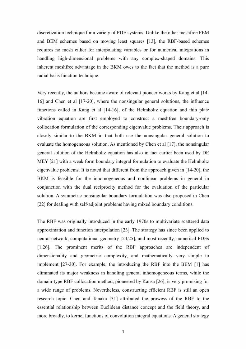
reaching the minimum relative error value. Fig. 6 displays the average relative error
curve of the homogeneous Neumann Helmholtz problem with the same analytical
solution and square domain shown in Fig. 1. It is observed that like the Dirichlet
cases, the convergence behaviour of the Neumann problem is very sound and stable
with a convergence rate of 50.7. After reaching the minimum values, the error curves
have the oscillations of small range in all these cases. Numerically, one concludes that
the BKM has the super-convergent speed in the present cases.
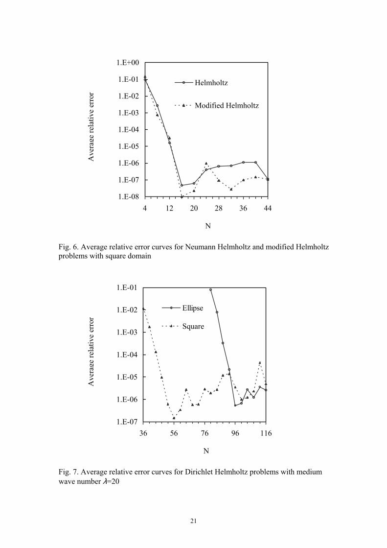
To investigate the Helmholtz problems with the medium and high wave numbers,
consider the Dirichlet problem with analytical solution
11

( ) ( ) ( yxyxu )λλ cossin, += . (29)
Figs. 7 and 8 respectively show the error curves for the cases involving wave number
λ=20 and λ=100. It is found that in each figure, the BKM requires more knots to
produce the solution of acceptable accuracy for the case with ellipse domain than for
that with square domain. By comparing the results of Figs. 7 and 8, it is also noted
that the higher the wave number, the more knots are necessary to suffice accuracy.
The convergence curves of both cases are also quite oscillatory and show that the
severe ill-conditioning seriously affects the solution accuracy.
To clearly expose the wave property of the Helmholtz problem, Fig. 9 illustrates the
solution surface with wave number λ=20 in a square domain. Figs. 10 and 11 present
the relative error surfaces using 12 and 18 BKM boundary knots, respectively, which
were generated with the relative errors at 101×101 knots uniformly covering the unit
square. It is seen that with the exception of the relatively less accurate solutions at
very few knots, the BKM solution accuracy as a whole is quite high even with 12
boundary knots.
Case 2. 2D modified Helmholtz problems
The BKM is tested to the modified Helmholtz problems with analytical solution
( ) yxeyxu +=, . (30)
λ in the corresponding non-singular general solution (13) is here equivalent to 2 .
As a matter of interest, Fig. 12 shows the accurate solution surface of this Dirichlet
problem with square domain. Figs. 13 and 14 display the corresponding relative error
surfaces using the BKM with 8 and 20 boundary knots, respectively, where the error
surfaces were also yielded by relative errors at 101×101 knots uniformly covering the
unit square. It is surprising to note that the error surface of the 8 boundary knots BKM
12

is very smooth and regular, while, in contrast, that of BKM using 20 boundary knots
is very random. In both cases, highly accurate solutions were obtained.
The relative error behaviours against the knot numbers are clearly illustrated in Figs.
5, 6 and 15, respectively. It is seen from Fig. 15 that the BKM converges stably and
quickly in both Dirichlet cases involving ellipse and square domains. Furthermore,
Fig. 5 shows that the BKM performs equally well for the Neumann case, while Fig. 6
demonstrates that the BKM is robust and yields very accurate solutions for the
Dirichlet modified Helmholtz problem with relatively complex-shaped domain, a
square with an elliptical hole.
Case 3. 2D convection-diffusion problems
Next, we look into the BKM solution of the steady Dirichlet convection-diffusion
problems with analytical solution
( ) yx eeyxu −− +=, . (31)
The parameter µ in the non-singular general solution (22) is 22 for this case. The
BKM average relative error curves are given respectively in Fig. 5 for square domain
with an elliptical hole and Fig. 16 for both square and elliptical domains. It is seen
from Fig. 16 that the BKM performs better in square domain case than in elliptical
domain case. In the latter, the visible oscillation is observed for the larger numbers of
knots. It is, however, worth stressing that the BKM solutions in both cases are very
accurate. For the case involving square domain with elliptical hole, the BKM solution
converges very quickly as shown in Fig. 5. From the above experiments, the boundary
geometry seems not to have strong affect on the convergence and accuracy of the
BKM solution.
Case 4. 3D Helmholtz, modified Helmholtz, and convection-diffusion problems
Finally, we examine the 3D Dirichlet problems under unit sphere domain. The
analytical solutions are respectively
13

( ) ( ) ( ) (zyxzyxu coscossin,, = ) (32)
for the Helmholtz equation,
( ) zyx eeezyxu ++=,, (33)
for the modified Helmholtz equation, and
( ) zyx eeezyxu −−− ++=,, (34)
for the convection-diffusion equation. The characteristic parameters λ and µ in the
corresponding non-singular solutions (13), (20) and (22) are 3 , 3 , and 23 ,
respectively. The same Helmholtz and convection-diffusion cases involving a unit
cube have been investigated in [33]. Here they are reanalysed to show the
convergence and stability of the BKM through the curves of the relative errors against
knot numbers. The average relative error curves of the BKM solutions at the interior
knots of x=0,0.2,-0.4,0.5,-0.6,0.8,-0.9, y=z=0 are plotted in Fig. 17. It is noted that the
BKM boundary knots on the sphere surface were taken randomly.
It is found that the accuracy of all three cases is constantly improved as the
incremental BKM boundary knots. It is especially stressed that the programming
effort for 2D and 3D cases makes no difference for the BKM. The present 3D
experiments further confirm the excellent accuracy and efficiency of the BKM.
4. Concluding remarks
It is revealed from the forgoing relative error curve figures that with the increasing
number of sampling BKM boundary nodes, the calculated results do exhibit
convergence trend in all tested cases. Moreover, the convergence is quick and stable
in general. The efficacy of the BKM formulation is validated for the Helmholtz,
14

modified Helmholtz, and convection-diffusion problems, which are practically
important in a broad range of physical and engineering areas.
The present study was undertaken to numerically examine the convergence behaviour
of the BKM. The given experiments meet this objective. The BKM has neither
singular integration, slow convergence and mesh in the DR-BEM nor artificial
boundary outside physical domain in the MFS. These merits lead to excellent
performances in computational accuracy, efficiency and stability as shown in the
preceding section 3. On the other hand, the method is extremely simple to learn and
easy to program, especially for complicated shapes and higher dimensions. In shark
contrast, the MFS suffers a severe difficulty in handling complex geometry problems
[7,37] due to a controversial artificial boundary.
More theoretical analysis and experimental studies of the BKM should be beneficial.
For example, we do not know by now if the BKM can be applied to exterior
problems. We also do not have a mathematical proof of the solvability and
convergence of the method although it always succeeds in various experiments. Some
issues concerning the optimal location of the knots and the choice of the radial basis
function in the context of the BKM for the inhomogeneous problem has yet to be
investigated. This is the subject of the future study.
Acknowledgements
The work described in this paper was partially supported by a grant from the Research
Grants Council of the Hong Kong Special Administrative Region, China (Project No.
CityU 1178/02P). The first author was then a visiting research fellow to the
Mathematics Department of City University of Hong Kong.
References
1. D. Nardini, C.A. Brebbia, A new approach to free vibration analysis using
boundary elements. Appl. Math. Modeling, 7 (1983) 157-162.
15

2. P.W. Partridge, C.A. Brebbia, L.W. Wrobel, The Dual Reciprocity Boundary
Element Method, Comput. Mech. Publ., Southampton, UK, 1992.
3. T. Yamada, L.C. Wrobel, H. Power, On the convergence of the dual reciprocity
boundary element method, Eng. Anal. BEM, 13 (1994) 291-298.
4. M.A. Golberg, C.S. Chen, The method of fundamental solutions for potential,
Helmholtz and diffusion problems. In Boundary Integral Methods - Numerical and
Mathematical Aspects, ed. M.A. Golberg, pp. 103-176, Comp. Mech. Publ., 1998.
5. A. Bogomolny, Fundamental solutions method for elliptic boundary value
problems, SIAM J. Numer. Anal. 22(4) (1985) 644-669.
6. J. Li, Mathematical justification for RBF-MFS, Engng. Anal. Bound. 25(10) (2001)
897-901.
7. J.H. Kane, Boundary Element Analysis in Engineering Continuum Mechanics,
Prentice Hall, New Jersey, 1994.
8. K. Balakrishnan, P.A. Ramachandrant, A particular solution Trefftz method for
non-linear Poisson problems in heat and mass transfer, J. Comput. Phy. 150 (1999)
239-267.
9. P.W. Partridge, B. Sensale, The method of fundamental solutions with dual
reciprocity for diffusion and diffusion-convection using subdomains, Eng. Anal.
BEM, 24 (2000) 633-641.
10. T. Kitagawa, Asymptotic stability of the fundamental solution method. J. Comput.
Appl. Math. 38 (1991) 263-269.
11. W. Chen, M. Tanaka, New insights in boundary-only and domain-type RBF
methods, Int. J. Nonlinear Sci. Numer. Simulation, 1(3) (2000) 145-152.
12. W. Chen, M. Tanaka, A meshfree, integration-free, and boundary-only RBF
technique, Comput. Math. Appls. 43 (2002) 379-391.
13. P. Mendonca, C. Barcellos, A. Durate, Investigations on the hp-Cloud method by
solving Timoshenko beam problems, Comput. Mech. 25 (2000) 286-295.
14. S. W. Kang, J. M. Lee, Y. J. Kang, Vibration analysis of arbitrarily shaped
membranes using non-dimensional dynamic influence function, J. Sound Vibr.,
221(1) (1999) 117-132.
15. S. W. Kang, J. M. Lee, Eigenmode analysis of arbitrarily shaped two-dimensional
cavities by the method of point-matching, J. Acoust. Soc. Am., 107(3) (2000)
1153-1160.
16

16. S. W. Kang, J. M. Lee, Free vibration analysis of arbitrarily shaped plates with
clamped edges using wave-type functions, J. Sound Vibr. 242(1) (2001), 9-26.
17. J. T. Chen, M. H. Chang, K. H. Chen, S. R. Lin, The boundary collocation method
with meshless concept for acoustic eigenanalysis of two-dimensional cavities
using radial basis function, J. Sound Vibr., 257(4) (2002), 667-711.
18. J. T. Chen, I. L. Chen, K. H. Chen, Y. T. Lee, Comments on “Free vibration
analysis of arbitrarily shaped plates with clamped edges using wave-type
function”, Comput. Mech., (in press), 2002.
19. J. T. Chen, M. H. Chang, I. L. Chung, Y. C. Cheng, Comment on “Eigenmode
analysis of arbitrarily shaped two-dimensional cavities by the method of point
matching”, J. Acoust. Sco. Am. 111(1) (2002), 33-36.
20. J. T. Chen, M. H. Chang, K. H. Chen, I. L. Chen, Boundary collocation method
for acoustic eigenanalysis of three-dimensional cavities using radial basis
function, Comput. Mech., 29 (2002), 392-408.
21. G. DE MEY, A simplified integral equation method for the calculation of the
eigenvalues of Helmholtz equation, J. Acoust. Soc. Am., 11 (1977) 1340-1342.
22. W. Chen, Symmetric boundary knot method, Engng. Anal. Bound. Elem., 26(6)
(2002) 489-494.
23. R.L. Hardy, Multiquadratic equations for topography and other irregular surfaces,
J. Geophys. Res. 176 (1971) 1905-1915.
24. M. Powell, Recent advances in Cambridge on radial basis functions. The 2nd
International Dortmunt Meeting on Approximation Theory, 1998.
25. R. Schaback, H. Wendland, Numerical techniques based on radial basis functions.
In Curve and Surface Fitting: Saint-Malo 1999, ed. A. Cohen et al., pp. 359-374,
Vanderbilt University Press, 2000.
26. E.J. Kansa, Multiquadrics: A scattered data approximation scheme with
applications to computational fluid dynamics. Comput. Math. Appl. 19 (1990)
147-161.
27. X. Zhang X.H. Liu, K.Z. Song, M.W. Lu, Least-square collocation meshless
method, Int. J. Numer. Methds. Engng., 51(9) (2001) 1089-1100.
28. X. Zhang, M.W. Lu, J.L. Wegner, A 2-D meshless model for jointed rock
structures, Int. J. Numer. Methds. Engng. 47(10) (2000) 1649-1661.
29. X. Zhang, K.Z. Song, M.W. Lu, Meshless Methods Based on Collocation with
Radial Basis Functions, Comput. Mech. 26(4) (2000) 333-343.
17

30. Y.C. Hon, X.Z. Mao, A radial basis function method for solving options pricing
model. Financial Eng. 81(1) (1999) 31-49.
31. W. Chen, M. Tanaka, Relationship between boundary integral equation and radial
basis function, in The 52th Symposium of JSCME on BEM, ed. M. Tanaka, Tokyo,
2000.
32. W. Chen, W. He, A note on radial basis function computing, Int. J. Nonlinear
Modelling Sci. Eng., 1 (2001) 59-65.
33. Y.C. Hon, W. Chen, Boundary knot method for 2D and 3D Helmholtz and
convection-diffusion problems with complicated geometry, (in press), 2002.
34. M. Golberg, C.S. Chen, H. Bowman, H. Power, Some comments on the use of
radial basis functions in the dual reciprocity method, Comput. Mech. 21 (1998)
141-148.
35. M. Zerroukat, H. Power, C.S. Chen, A numerical method for heat transfer
problems using collocation and radial basis function, Int. J. Numer. Method Eng.
42 (1998) 1263-1278.
36. H. Ding, C. Shu, K.S. Yeo, Simulation of natural convection in an eccentric
annulus between a square outer cylinder and a circular inner cylinder using the
local MQ-DQ method, (submitted), 2002.
37. K. Balakrishnan, P.A. Ramachandran, The method of fundamental solutions for
linear diffusion-reaction equations, Math. Comput. Modelling. 31 (2000) 221-237.
18

19

1.E-10
1.E-09
1.E-08
1.E-07
1.E-06
1.E-05
1.E-04
1.E-03
1.E-02
1.E-01
1.E+00
4 12 20 28 36 4
N
4
Ellipse
Square
Ave
rage
rela
tive
erro
r
Fig. 4. Average relative error curves for Dirichlet Helmholtz problems with elliptical and square domains
1.E-09
1.E-08
1.E-07
1.E-06
1.E-05
1.E-04
1.E-03
1.E-02
1.E-01
1.E+00
7 11 15 19 23 27 31 35
N
Helmhotlz
Modified Helmholtz
Convection-diffusion
Ave
rage
rela
tive
erro
r
Fig. 5. Average relative error curves for Dirichlet Helmholtz, modified Helmholtz, and convection-diffusion problems with square domain with elliptical hole
20
1.E-08
1.E-07
1.E-06
1.E-05
1.E-04
1.E-03
1.E-02
1.E-01
1.E+00
4 12 20 28 36 4
N
4
Helmholtz
Modified Helmholtz
Ave
rage
rela
tive
erro
r
Fig. 6. Average relative error curves for Neumann Helmholtz and modified Helmholtz problems with square domain
1.E-07
1.E-06
1.E-05
1.E-04
1.E-03
1.E-02
1.E-01
36 56 76 96 116
N
Ellipse
Square
Ave
rage
rela
tive
erro
r
Fig. 7. Average relative error curves for Dirichlet Helmholtz problems with medium wave number λ=20
21

1.E-06
1.E-05
1.E-04
1.E-03
1.E-02
1.E-01
1.E+00
116 296 476 656 836
N
Ellips
Square
Ave
rage
rela
tive
erro
r
Fig. 8. Average relative error curves for Dirichlet Helmholtz problems with high wave number λ=100
22

23

24

Ave
rage
rela
tive
erro
r
1.E-09
1.E-08
1.E-07
1.E-06
1.E-05
1.E-04
1.E-03
1.E-02
1.E-01
1.E+00
4 12 20 28 36 4
N
4
Ellipse
Square
Fig. 15. Average relative error curves for Dirichlet modified Helmholtz problem with elliptical and square domains
25

1.E-10
1.E-09
1.E-08
1.E-07
1.E-06
1.E-05
1.E-04
1.E-03
1.E-02
1.E-01
4 12 20 28 36 4
N
4
Ellipse
Square
Ave
rage
rela
tive
erro
r
Fig. 16. Average relative error curves for Dirichlet convection-diffusion problem with elliptical and square domains
1.E-08
1.E-07
1.E-06
1.E-05
1.E-04
1.E-03
1.E-02
1.E-01
5 25 45 65 85 105 125
N
HelmholtzModified HelmholtzConvection-diffusion
Ave
rage
rela
tive
erro
r
Fig. 17. Average relative error curve for Dirichlet Helmholtz, modified Helmholtz and convection-diffusion problems with 3D sphere domain
26